NTNU Fakultet for naturvitenskap og teknologi Norges teknisk-naturvitenskapelige Institutt for kjemisk prosessteknologi universitet

Calculation of Vapor-Liquid Equilibria

for Methanol-Water Mixture using Cubic-Plus-Association

Equation of State

Project work in the subject KP8108 ”Advanced Thermodynamics”

Ardi Hartono Inna Kim

2004

2

Table of content

INTRODUCTION

1. THERMODYNAMIC FRAMEWORK

1.1. Thermodynamics of vapor-liquid equilibria

1.2. Fugacity criteria for phase equilibria

1.3. Fugacity coefficient

1.4. Calculation of fugacity

1.5. Fugacity of pure fluid

2. VAPOR-LIQUID EQUILBRIA WITH EQUATIONS OF STATE

2.1. Virial equations of state

2.2. Analytical equations of state

2.2.1. Estimation of a, b and c parameters for the Soave-Redlich-Kwong EoS

2.2.2. Mixing rules

2.3. Nonanalytic equations of state

2.3.1. Associating and polar fluids (Chemical theory EoS)

2.4. Summary on equations of state

3. THERMODYNAMIC PROPERTIES FROM VOLUMETRIC DATA

3.1. The Helmholz energy and its derivatives

3.2. Calculation of the derivatives of the Helmholz energy

4. THE CPA EQUATION OF STATE

4.1. Association energy and volume parameters

4.2. Association term in CPA EoS

4.2.1. Fraction of nonbonded associating molecules, XA

4.2.2. Association schemes

4.3. Chemical potential and fugacity coefficient from CPA EoS

4.3.1. Volume from CPA EoS

4.3.2. Newton-Raphson technique in calculating volume in CPA EoS

4.4. Flash calculation

4.4.1. Bubble-point pressure calculation

4.5. Results and discussion

LIST OF SYMBOLS

REFERENCES

APPENDICES

3

INTRODUCTION

Vapor-liquid equilibria are the fundamental properties whose knowledge is required, for

example, in the design of separation columns in chemical industries. Many experiments are

necessary to obtain such equilibrium data, at least for binary systems, where non-idealities in

both phases must be determined. Therefore further improvements to theoretical models for

describing and predicting these non-idealities are indispensable.

At low pressure, deviations from ideal behaviour are due mainly to the liquid phase. The

association of one or more components in a liquid mixture and the chemical forces due to

electrical charge exchange between an associating and an active compound influence strongly

the excess properties of associated solutions and the fluid phase equilibria. These effects are

in many cases stronger than those due to physical forces. It is therefore advantageous to treat

chemical and physical interactions separately in theoretical models for the excess properties

of associated solutions (Nath A, 1981).

Equations of state have traditionally been applied to modelling systems with non-polar and

slightly polar compounds. For associating compounds, however, a new concept has evolved

in recent years with the development of equations of state combining the physical effects from

the classical models and a chemical contribution. An example of this new concept is an

equation of state abbreviated CPA – Cubic Plus Association presented by Kontogeorgis et al.

(1996). CPA has been applied extensively to the modelling of vapor-liquid equilibria (VLE)

for alcohol-hydrocarbon systems, in correlating liquid-liquid equilibria (LLE) for alcohol-

hydrocarbon mixtures, as well as for binary aqueous systems containing hydrocarbons It has

also been applied to the multicomponent systems, namely prediction of VLE and LLE for

ternary mixtures consisting of water-alcohol-hydrocarbons, including the prediction of the

partitioning of methanol between water and hydrocarbons. (Derawi et al., 2003).

In this work we will correlate the experimental VLE data for the methanol-water system using

simplified CPA EoS.

4

1. THERMODYNAMIC FRAMEWORK

1.1. Thermodynamics of vapor-liquid equilibria

We are concerned with a liquid mixture that, at temperature T and pressure P, is in

equilibrium with a vapor mixture at the same temperature and pressure. The quantities of

interest are the temperature, the pressure, and the composition of both phases. Given some of

these quantities, our task is to calculate the others.

Phase equilibria govern the distribution of molecular species between the vapor and liquid

phases. The equilibrium conditions for phase equilibria can be derived in the simplest way

using the Gibbs energy G. The Gibbs free energy of a mixture is a function of temperature,

pressure and composition, and its total derivative can be written in terms of partial derivatives

in the independent variables as (Stromberg, 2003):

1 2, , 1 2, , , ,

...i i j j

P n T n P T n P T n

G G G GdG dT dP dn dnT P n n

⎛ ⎞ ⎛ ⎞⎛ ⎞ ⎛ ⎞∂ ∂ ∂ ∂⎟ ⎟⎜ ⎜⎟ ⎟⎜ ⎜ ⎟ ⎟= + + +⎜ ⎜⎟ ⎟⎜ ⎜ ⎟ ⎟⎟ ⎟ ⎜ ⎜⎜ ⎜ ⎟ ⎟⎜ ⎜⎝ ⎠ ⎝ ⎠∂ ∂ ∂ ∂⎝ ⎠ ⎝ ⎠ (1.1)

where ni is the number of moles of all components, nj is the number of moles of all

components except one which is under consideration (i). At the constant temperature and

pressure Eq (1.1) is reduced to

, 1 1 2 2....P TdG dn dnμ μ= + or ( ), ,P T i i P TdG dnμ= ∑ (1.2)

here iμ is the chemical potential of component i , , , j ì

ii P T n

Gn

μ≠

⎛ ⎞∂ ⎟⎜ ⎟=⎜ ⎟⎜ ⎟⎜∂⎝ ⎠.

For the equilibrium at constant P and T, the Gibbs energy is minimized and mathematically

the minimum means dG=0 (Elliott, 1999). Therefore, Eq (1.1) is equal to 0 at a minimum and

for a closed system all dni are zero. Thus,

, 0T PdG = (1.3)

In the two-phase system is at equilibrium, then application of the Eq (1.2) yields

, 0V V L LT P i i i i

i i

dG dn dnμ μ= + =∑ ∑ (1.4)

here superscripts V and L denote the vapor and liquid phases respectively.

5

For the closed system without chemical reaction V Li idn dn=− , so it follows that

V Li iμ μ= (1.5)

Thus, the general equilibrium criteria for a closed, heterogeneous system consisting of π

phases and n components is that at equilibrium:

(1) (2) ( )...T T T π= = = (1.6)

(1) (2) ( )...P P P π= = = (1.7)

(1) (2) ( )1 1 1... πμ μ μ= = =

…

(1) (2) ( )...n n nπμ μ μ= = =

It says that at equilibrium, the temperature, pressure and chemical potentials of all species are

uniform over the whole system.

The chemical potential does not have an immediate equivalent in the physical world and it is

therefore desirable to express the chemical potential in terms of some auxiliary function that

might be more easily identified with physical reality. In the thermodynamic treatment of

phase equilibria, auxiliary thermodynamic functions such as fugacity coefficient and the

activity coefficient are often used. These functions are closely related to Gibbs energy.

1.2. Fugacity criteria for phase equilibria

The fugacity of component i in a mixture is defined as (Elliott, 1999):

ln i iRTd f dμ= at constant T (1.8)

where fi is the fugacity of component i in a mixture and μi is the chemical potential of the

component.

The equality of chemical potentials at equilibrium, Eq (1.5), can easily be interpreted in terms

of fugacity. By integrating Eq (1.8) as a function of composition at fixed T from a state of

pure i to a mixed state, we find

00lnV

V ii i

i

fRTf

μ μ− = (1.9)

where 0iμ and 0

if are for the pure fluid at the system temperature. Writing an analogous

expression for the liquid phase, and equating the chemical potentials using Eq (1.5), we find

6

ln 0V

V L ii i L

i

fRTf

μ μ⎛ ⎞⎟⎜ ⎟− = =⎜ ⎟⎜ ⎟⎜⎝ ⎠

(1.10)

Then the condition for phase equilibria can be written as:

V Li if f= (1.11)

Eq (1.11) gives us a useful result. It tells us that the equilibrium condition in terms of

chemical potentials can be replaced without loss of generality by an equation in terms of

fugacities.

1.3. Fugacity coefficient

G.N. Lewis defined the fugacity of component i in a mixture is defined by:

ln idG VdP RTd f= ≡ at constant T (1.12)

For a real fluid, the volume is given by /V ZRT P= , thus:

dPdG RTZP

= (1.13)

for an ideal gas, we may substitute Z=1 into Eq. (1.13) and obtain

lnig dPdG RT RTd PP

= = (1.14)

Comparing Eqs (1.13) and (1.14) we see that

( ) / ln( / )igd G G RT d f P− = (1.15)

Integrating this equation at low pressure at constant temperature, we have for the left-hand

side:

( ) ( ) ( )0

0

1 1( )igP

ig ig ig

P P

G Gd G G G G G G

RT RT RT=

−⎡ ⎤− = − − − =⎢ ⎥⎣ ⎦∫ (1.16)

because (G-Gig) approaches zero at low pressure. Integrating the right-hand side of Eq.(1.12),

we have

0

ln lnP P

f fP P =

⎛ ⎞ ⎛ ⎞⎟ ⎟⎜ ⎜−⎟ ⎟⎜ ⎜⎟ ⎟⎜ ⎜⎝ ⎠ ⎝ ⎠

To complete the definition of fugacity, we define the low pressure limit,

0lim 1P

fP→

⎛ ⎞⎟⎜ =⎟⎜ ⎟⎜⎝ ⎠ (1.17)

Here the ratio f/P is defined as the fugacity coefficient φ.

7

( ) ln lnigG G f

RT Pϕ

−= = (1.18)

In practice, we evaluate the fugacity coefficient, and then calculate the fugacity by

f Pϕ=

1.4. Calculation of fugacity

The fugacity of component i, fi, is related to its departure function chemical potential as:

ln ( , , )ri iRT T P nϕ μ= (1.19)

where

,

,

, ,

( , , )j ì

r Pr Pi

i T P n

GT P nn

μ≠

⎛ ⎞∂ ⎟⎜ ⎟=⎜ ⎟⎜ ⎟⎜ ∂⎝ ⎠ (1.20)

It is simply another way of characterizing the Gibbs departure function at a fixed T, P. For an

ideal gas, the fugacity will equal the pressure, and the fugacity coefficient will be unity. For

representation of the P-V-T data in the form of Z=f(T,P), the fugacity coefficient is evaluated

using Eqs (1.13), (1.14) from:

( ) ( )

0 0

1 1ln lnig P P

igG G f ZV V dP dP

RT P RT Pϕ

− ⎛ ⎞ ⎛ ⎞−⎟ ⎟⎜ ⎜= = = − =⎟ ⎟⎜ ⎜⎟ ⎟⎜ ⎜⎝ ⎠ ⎝ ⎠∫ ∫ (1.21)

or the equivalent form for P-V-T data in the form Z=f(T,V):

( ) ( )

0

11ln ln ( 1) lnigG G Zf d Z Z

RT P RT

ρ

ϕ ρρ

− ⎛ ⎞ −⎟⎜= = = + − −⎟⎜ ⎟⎜⎝ ⎠ ∫ (1.22)

which is the form used for the cubic equations of state.

The chemical potential of a component, μi, is the partial molar Gibbs energy, but it is also a

partial derivative of other properties:

, , , , , , , ,j ì j ì j ì j ì

ii i i iT P n T V n S V n S P n

G A U Hn n n n

μ≠ ≠ ≠ ≠

⎛ ⎞ ⎛ ⎞ ⎛ ⎞ ⎛ ⎞∂ ∂ ∂ ∂⎟ ⎟ ⎟ ⎟⎜ ⎜ ⎜ ⎜⎟ ⎟ ⎟ ⎟= = = =⎜ ⎜ ⎜ ⎜⎟ ⎟ ⎟ ⎟⎜ ⎜ ⎜ ⎜⎟ ⎟ ⎟ ⎟⎜ ⎜ ⎜ ⎜∂ ∂ ∂ ∂⎝ ⎠ ⎝ ⎠ ⎝ ⎠ ⎝ ⎠ (1.23)

So, when volume rather than pressure is fixed, the fugacity coefficients maybe also

derived from the total residual Helmholz energy, i.e. the Helmholz function of the mixture,

given as a function of temperature T, total volume V, and the vector of mixture mole numbers

n, minus that equivalent ideal gas mixture at (T, V, n). However, traditionally the definition of

the fugacity coefficient in Eq. (1.19) is not changed in the transition from G to A, it describes

8

the departure between the real fluid and ideal gas at given pressure, not at given volume. So,

we have to find Ar at fixed pressure. Using known expression ( ) ,/

T nA V P∂ ∂ =− and taking

into account that the pressure is by definition the same in the ideal gas and the real fluid, but

volumes are different, we can write:

( )( ) ( ) ( )

( )

( , ( ), ) ( , ( ), ) ( , ( ), )

lnig

r ig ig

V P V P V Pig ig

V P

A T V P n A T V P n A T V P n

nRTdv dv dv nRT Zv

π π π π∞ ∞

= − =

⎛ ⎞⎟⎜= − − = − −⎟⎜ ⎟⎜⎝ ⎠∫ ∫ ∫ (1.24)

Then

, , ,

1ln ln lnj ì

Vr

ii i iT V T V n

A PV Zn RT n RT v n

πϕ

≠∞

⎡ ⎤⎛ ⎞ ⎛ ⎞⎛ ⎞∂ ∂⎢ ⎥⎟ ⎟⎟ ⎜ ⎜⎜ ⎟ ⎟⎟= − = − −⎜ ⎜⎜ ⎢ ⎥⎟ ⎟⎟ ⎜ ⎜⎜ ⎟ ⎟ ⎟⎜ ⎜ ⎜∂ ∂⎝ ⎠ ⎝ ⎠ ⎝ ⎠⎢ ⎥⎣ ⎦

∫ (1.25)

The fundamental problem is to relate these fugacities to mixture composition. The fugacity of

a component is a mixture depends on the temperature, pressure, and composition of that

mixture. In principle any measure of composition can be used. For a mixture of ideal gases,

1iϕ = .

For the vapor phase, the composition is nearly always expressed by the mole fraction y. To

relate Vif to temperature, pressure, and mole fraction, it is useful to introduce the vapor-phase

fugacity coefficient Viϕ :

V

V ii

i

fy P

ϕ = (1.26)

which can be calculated from vapor phase PVT-y data, usually given by an equation of state.

The fugacity coefficient depends on temperature and pressure and, in a multicomponent

mixture, on all mole fractions in the vapor phase, not just yi. The fugacity coefficient is, by

definition, normalized such that as 0P → , 1Viϕ → for all I (see Ch.1.1.1.b). At low pressure,

therefore, it is usually a good assumption to set 1Viϕ = .

The fugacity of component i in the liquid phase is generally calculated by one of two

approaches: the equation of state approach or the activity coefficient approach.

9

Activity coefficient approach: The fugacity of component i in the liquid phase is related to

the composition of that phase through the activity coefficient iγ . To develop expressions for

activity coefficients and their composition derivatives, we write the model expression for the

total excess Gibbs energy, Etn g , replacing mole fractions xi by mole numbers ni. Activity

coefficients are then found from

,

lnE

ti

i T P

n gn RT

γ⎛ ⎞∂ ⎟⎜ ⎟= ⎜ ⎟⎜ ⎟⎜∂ ⎝ ⎠

(1.27)

Activity coefficient iγ is related to xi and to standard state fugacity 0if by

10

( , , , ,...)( , , 1)

Li i i

ii i i i i

a f T P x xx x f T P x

ϕγ

ϕ≡ = =

= (1.28)

where ai is the activity of component i. The standard-state fugacity 0if is the fugacity of

component i at the same temperature of the system and at some arbitrary chosen pressure and

composition.

While there are some important exceptions, activity coefficients for most typical solutions of

non-electrolytes are based on a standard state where, for every component i, 0if is the fugacity

of pure liquid i at system temperature and pressure, i.e. the arbitrary chosen pressure is the

total pressure P, and the arbitrary chosen composition is xi = 1. Whenever the standard-state

fugacity is that of the pure liquid at system temperature and pressure, we obtain the limiting

relation that 1iγ → as 1ix → (Raoult’s law standard state).

Equation of state approach: The liquid-phase fugacity coefficient, Liϕ , is calculated using Eq.

(1.25) just as for vapor. The only significant consideration is that the liquid compressibility

factor must be used.

When we extend the equation of state to mixtures, the basic form of the equations do not

change. The fluid properties of the mixture are written in terms of the same equation of state

parameters as fore the pure fluids; however, the equations of state parameters are functions of

compositions. The equations we use to incorporate compositional dependence into the

mixture constants are termed the mixing rules.

We will use the Equation of state approach in this work for methanol-water VLE calculation.

10

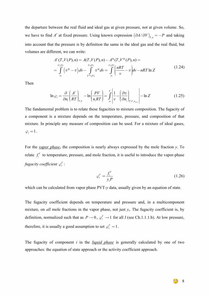
1.5. Fugacity of pure liquid

To calculate the fugacity for liquid, used in the Eq.(1.28), consider Fig. 1.1. Point A

represents a vapor state, point B – saturated vapor, point C – saturated liquid, and point D

represents a liquid. Calculation of the saturation fugacity may be carried out by any of the

methods for calculation of vapor fugacities. Methods differ slightly on how the fugacity is

calculated between points C and D. There are two primary methods for calculating this

fugacity change. They are Poynting method and the equation of state method.

The Poynting method applies Eq (1.12) between saturation (points B, C) and point D. The

integral is

lnD

sat

PDsat

P

fRT VdPf

= ∫ (1.29)

Fig. 1.1. Schematic for calculation of Gibbs energy and fugacity changes

at constant temperature for a pure liquid (Elliott, 1999)

Since liquid are fairly incompressible for Tr<0.9, the volume is approximately constant over

the interval of integration, and may be removed from the integral, with the resulting Poynting

correction becoming

( )exp

L sat

sat

V P Pff RT

⎛ ⎞− ⎟⎜ ⎟⎜= ⎟⎜ ⎟⎜ ⎟⎟⎜⎝ ⎠ (1.30)

Volume

Psat

PD

sat Vsat L

A

BC

D Pressure

T<Tc

11

Then the fugacity for the liquid is calculated by

( )0, expL sat

L sat satV P P

f PRT

ϕ⎛ ⎞− ⎟⎜ ⎟⎜= ⎟⎜ ⎟⎜ ⎟⎟⎜⎝ ⎠

(1.31)

Saturate volume can be estimated within a few percent error using the Rackett equation 0.2857(1 )rTsatL

c cV V Z −= (1.32)

The Poynting correction is essentially unity for many compounds near the room T and P; thus,

it is frequently ignored. sat satf Pϕ≈

12

2. VAPOR-LIQUID EQUILIBRIA WITH EQUATIONS OF STATE

The volumetric properties of a pure fluid in a give state are commonly expressed with the

compressibility factor Z, which can be written as a function of T and P or of T and V:

( , )PPVZ f T PRT

≡ = (2.1)

( , )vf T V= (2.2)

where V is the molar volume, P is the absolute pressure, T is the absolute temperature and R

is so called universal gas constant. For an ideal gas, 1Z = . For real gases, Z is somewhat less

than 1 except at high temperatures and pressures.

An algebraic relation between P, V and T is called an EoS. Many equations of state have been

proposed for engineering applications. From equation of state we get not only PVT

information but, from the interrelations provided by classical thermodynamics, departure

functions from ideal gas behaviour and phase equilibria can be calculated. The equations of

state may be classified as follows:

- the virial equation;

- semi theoretical EoS which are cubic or quadric in volume, and therefore whose

volumes can be found analytically from specified P and T;

- non analytic equations

The virial equation can be derived from molecular theory, but is limited in its range of

applicability. It can represent modest deviations from ideal gas behaviour, but not liquid

properties. Semi theoretical EoS can represent both liquid and vapor behaviour over limited

ranges of temperature and pressure for many but not all substances. Finally, non analytic

equations are applicable over much broader ranges of P and T than are the analytic equations,

but they usually require many parameters that require fitting to large amount of data of

several properties. These models include semi theoretical models such as perturbation models,

chemical theory equations for strongly associating species, and crossover relations for a more

rigorous treatment of the critical region.

13

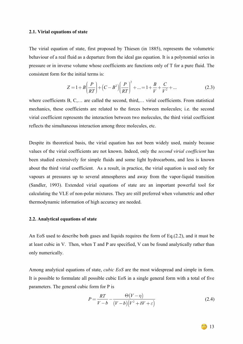
2.1. Virial equations of state

The virial equation of state, first proposed by Thiesen (in 1885), represents the volumetric

behaviour of a real fluid as a departure from the ideal gas equation. It is a polynomial series in

pressure or in inverse volume whose coefficients are functions only of T for a pure fluid. The

consistent form for the initial terms is:

( )2

221 ... 1 ...P P B CZ B C B

RT RT V V⎛ ⎞ ⎛ ⎞⎟ ⎟⎜ ⎜= + + − + = + + +⎟ ⎟⎜ ⎜⎟ ⎟⎜ ⎜⎝ ⎠ ⎝ ⎠

(2.3)

where coefficients B, C,… are called the second, third,… virial coefficients. From statistical

mechanics, these coefficients are related to the forces between molecules; i.e. the second

virial coefficient represents the interaction between two molecules, the third virial coefficient

reflects the simultaneous interaction among three molecules, etc.

Despite its theoretical basis, the virial equation has not been widely used, mainly because

values of the virial coefficients are not known. Indeed, only the second virial coefficient has

been studied extensively for simple fluids and some light hydrocarbons, and less is known

about the third virial coefficient. As a result, in practice, the virial equation is used only for

vapours at pressures up to several atmospheres and away from the vapor-liquid transition

(Sandler, 1993). Extended virial equations of state are an important powerful tool for

calculating the VLE of non-polar mixtures. They are still preferred when volumetric and other

thermodynamic information of high accuracy are needed.

2.2. Analytical equations of state

An EoS used to describe both gases and liquids requires the form of Eq.(2.2), and it must be

at least cubic in V. Then, when T and P are specified, V can be found analytically rather than

only numerically.

Among analytical equations of state, cubic EoS are the most widespread and simple in form.

It is possible to formulate all possible cubic EoS in a single general form with a total of five

parameters. The general cubic form for P is

( )

( )( )2

VRTPV b V b V V

η

δ ε

Θ −= −

− − + + (2.4)

14

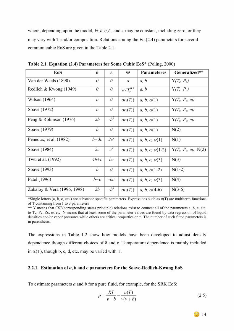
where, depending upon the model, , , ,b η δΘ , and εmay be constant, including zero, or they

may vary with T and/or composition. Relations among the Eq.(2.4) parameters for several

common cubic EoS are given in the Table 2.1.

Table 2.1. Equation (2.4) Parameters for Some Cubic EoS* (Poling, 2000)

EoS δ ε Θ Parameteres Generalized**

Van der Waals (1890) 0 0 a a, b Y(Tc, Pc)

Redlich & Kwong (1949) 0 0 0.5/ ra T a, b Y(Tc, Pc)

Wilson (1964) b 0 ( )ra Tα a, b, α(1) Y(Tc, Pc, ω)

Soave (1972) b 0 ( )ra Tα a, b, α(1) Y(Tc, Pc, ω)

Peng & Robinson (1976) 2b -b2 ( )ra Tα a, b, α(1) Y(Tc, Pc, ω)

Soave (1979) b 0 ( )ra Tα a, b, α(1) N(2)

Peneoux, et al. (1982) b+3c 2c2 ( )ra Tα a, b, c, α(1) N(1)

Soave (1984) 2c c2 ( )ra Tα a, b, c, α(1-2) Y(Tc, Pc, ω), N(2)

Twu et al. (1992) 4b+c bc ( )ra Tα a, b, c, α(3) N(3)

Soave (1993) b 0 ( )ra Tα a, b, α(1-2) N(1-2)

Patel (1996) b+c -bc ( )ra Tα a, b, c, α(3) N(4)

Zabaloy & Vera (1996, 1998) 2b -b2 ( )ra Tα a, b, α(4-6) N(3-6)

*Single letters (a, b, c, etc.) are substance specific parameters. Expressions such as α(T) are multiterm functions of T containing from 1 to 3 parameters ** Y means that CSP(corresponding states principle) relations exist to connect all of the parameters a, b, c, etc. to Tc, Pc, Zc, ω, etc. N means that at least some of the parameter values are found by data regression of liquid densities and/or vapor pressures while others are critical properties or ω. The number of such fitted parameters is in parenthesis.

The expressions in Table 1.2 show how models have been developed to adjust density

dependence though different choices of δ and ε. Temperature dependence is mainly included

in α(T), though b, c, d, etc. may be varied with T.

2.2.1. Estimation of a, b and c parameters for the Soave-Redlich-Kwong EoS

To estimate parameters a and b for a pure fluid, for example, for the SRK EoS:

( )( )

RT a Tpv b v v b

= −− +

(2.5)

15

The Eq. (2.5) is reshaped into a cubic polynomial:

3 2 2 0RT a RTb abv v b vp p p p

⎛ ⎞⎟⎜− + − − ⎟ − =⎜ ⎟⎜ ⎟⎜⎝ ⎠ (2.6)

At the critical point this equation must fulfil( )3 0cv v− = , that is 3 2 2 33 3 0c c cv v v vv v− + − = .

When compared term by term the two polynomials define a set of equations that can be

solved for a, b and vc:

3 ,cc

c

RTvp

= 2 23 ,cc

c c

RT bav bp p

= − − 3c

c

abvp

= (2.7)

The second equation is combined with the other two to yield ( )332 0c cv v b− + = , which is

solved for the positive root ( )1/32 1 cb v= − . In terms of critical temperature and pressure, for

any component i, this is equivalent to:

,

,

0.08664 c ii

c i

RTb

p=

2 2

0.042747 ci

c

R Tap

= (2.8)

At temperatures others than the critical

( ) ( )i ia T a Tα= (2.9)

where ( )i Tα is an non-dimensional factor which becomes unity at T=Tc. In SRK equation

(Soave, 1972):

0.5 0.51 (1 )i i rc Tα = + − (2.10)

Parameter ci can be connected directly with the acentric factor ωi of the related compounds by

20.480 1.547 0.176i i ic ω ω= + − (2.11)

Eqs. (2.9)-(2.11) yield the desired value of ai(T) of a given substance at any temperature:

( )( )2

( ) 1 1i i i ra T a c T= + − (2.12)

2.2.2. Mixing rules

The greatest utility of cubic equations of state is for phase equilibrium calculations involving

mixtures. The assumption inherent in such calculations is that the same equation of state used

for pure fluids can be used for mixtures if we have a satisfactory way of obtaining the mixture

parameters. This had been done for decades using the simple van der Waals one-fluid mixing

rules with one or two binary parameters

16

i j ij

i j ij

a x x a

b x x b

=

=

∑∑∑∑

(2.13)

In addition, combining rules are needed for the parameters aij and bij. The usual combining

rules are

(1 )

1 ( )(1 )2

ij ii jj ij

ij ii jj ij

a a a k

b b b l

= −

= + − (2.14)

where kij and lij are the binary interaction parameters obtained by fitting equation of state

predictions to experimental VLE data for kij or VLE and density data for kij and lij. We can

find different expressions for the binary interaction parameter in the literature. For example,

Wong et al. (1992) suggest that the combining rule for kij be of the form:

( )

( ) ( )2 /

1/ /

ijij

ii ii jj jj

b a RTk

b a RT b a RT

−− =

− + − (2.15)

Values for kij for various binary combinations are tabulated in the literature. In the absence of

the experimental data or literature values for kij, we may make a first-order approximation by

letting kij=0. For many mixtures lij is set equal to zero but there are situations where inclusion

of lij as a second interaction parameter leads to a better representation of VLE.

Nevertheless, this method was found to be satisfactory only for hydrocarbons, or

hydrocarbons and gases. It is only in recent years that new mixing and combining rules have

allowed the cubic equations of state to be used for accurate correlations, even for predictions

for more complicated mixtures involving organic chemicals.

2.3. Nonanalytical equations of state

The complexity of property behaviour cannot be described with high accuracy with the cubic

or quadric EoS that can be solved analytically for the volume, given T and P. Non analytical

equations of state include, for instance, strictly empirical BWR (Benedict-Webb-Rubin)

models and Wagner formulations, semi empirical formulations based on theory are

perturbation methods and chemical association models.

The technique of perturbation modelling uses reference values for systems that are similar

enough to the system of interest that good estimates of desired values can be made with small

17

corrections to the reference values. Perturbation terms, or those which take into account the

attraction between the molecules, have ranged from the very simple to extremely complex.

The simplest form is that of van der Waals which in terms of the Helmholz energy is

( )( )

, / /vdWr

AttA T V RT a RTV⎡ ⎤ =−⎢ ⎥⎣ ⎦ (2.16)

and which leads to an attractive contribution to the compressibility factor of

( ) /vdWAttZ a RTV=− (2.17)

This form would be appropriate for simple fluids though it has also been used with a variety

of reference expressions. The most complex expressions for normal substances are those used

in the BACK (Boublik-Alder-Chen-Kreglewski), PHCT (Perturbed Hard Chain Theory), and

SAFT (statistical associating fluid theory) EoS models. There general form is

( )

1 1

i jn mBACK

Att iji j

uZ r jDkT

ητ= =

⎡ ⎤ ⎡ ⎤⎢ ⎥ ⎢ ⎥=⎢ ⎥ ⎢ ⎥⎣ ⎦ ⎣ ⎦

∑∑ (2.18)

where the number of terms may vary, but generally n ~ 4-7 and m~10, the Dij coefficient and

τ are universal, and u and η are substance-dependent and may also be temperature dependent

as in the SAFT model.

2.3.1. Associating and polar fluids (Chemical theory EoS)

In many practical systems, the interactions between the molecules are quite strong due to

charge-transfer and hydrogen bonding. This occurs in pure components such as alcohol,

carboxylic acids, water and HF and leads to quite different behaviour of vapours of these

substances. Considering the interactions so strong that new “chemical species” are formed,

the thermodynamic treatment assumes that the properties deviate from an ideal gas mainly

due to the “speciation” plus some physical effect. It is assumed that all of the species are in

reaction equilibrium. Thus, their concentrations can be determined from equilibrium constants

having parameters such as enthalpies and entropies of reaction in addition to the usual

parameters for their physical interactions.

Associating (and solvating) species present a special problem with equations of state because

the occurrence of both weak chemical reactions and phase equilibrium. By proper coupling of

the contributions of the physical and chemical effects, the result is a closed form equation. A

similar formulation is made with the SAFT equation, where molecular level association is

18

taken into account by a reaction term that is added to the free energy term from reference,

dispersion, polarity, etc.

2.4. Summary on equations of state

To characterize small deviations from ideal gas behaviour the truncated virial equation with

either the second alone or the second and third coefficient should be used. Virial equations

should not be used for liquid phase.

For normal fluids, a generalized cubic EoS with volume translation should be used. All

models give equivalent and reliable results for saturated vapours except for the dimerizing

substances given above.

For polar and associating substances, a method based on four or more parameters should be

used. Cubic equations with volume translation can be quite satisfactory for small molecules,

though perturbation expressions are usually needed for polymers and chemical models for

carboxylic acid vapours.

19

3. THERMODYNAMIC PROPERTIES FROM VOLUMETRIC DATA

For any substance, regardless of whether it is pure or a mixture, most thermodynamic

properties of interest in phase equilibria can be calculated from thermal and volumetric

measurements. For a given phase, thermal measurements (heat capacities) give information

on how some thermodynamic properties vary with temperature, whereas volumetric

measurements give information on how thermodynamic properties vary with pressure or

density at constant temperature. Frequently it is useful to express a selected thermodynamic

function of a substance relative to that which the same substance has as an ideal gas at the

same temperature and composition and/or at some specified pressure of density. This relative

function is often called as residual function. The fugacity is a relative function because its

numerical value is always relative to that of an ideal gas at unit fugacity; in other words, the

standard-state fugacity 0if in Eq (1.28) is arbitrary set equal to some fixed value, usually 1

bar.

The thermodynamic function of our interest is the fugacity that is directly related to the

chemical potential. To obtain numerical values of the fugacity, we will find that an equation

of state is necessary. Since, such P, V, T, N relations are normally explicit in pressure, it will

be convenient to formulate the problem with T, V, N as the independent variables (Modell et

al., 1983). This conclusion suggests that a Legendre transform of the energy into T, V, n space

would be appropriate. Such a transform is the Helmholz energy, A:

A U TS= − (3.1)

i ii

dA SdT PdV dNμ=− − +∑ (3.2)

3.1. The Helmholz energy and its derivatives

Given an equation of state:

( , , )P P T v x= (3.3)

where x is the vector of mixture mole fractions, the textbook approach to calculate mixture

fugacity coefficients is by mean of an integrals given by Eq (1.21) or (1.25). Using the Eq.

(1.24)

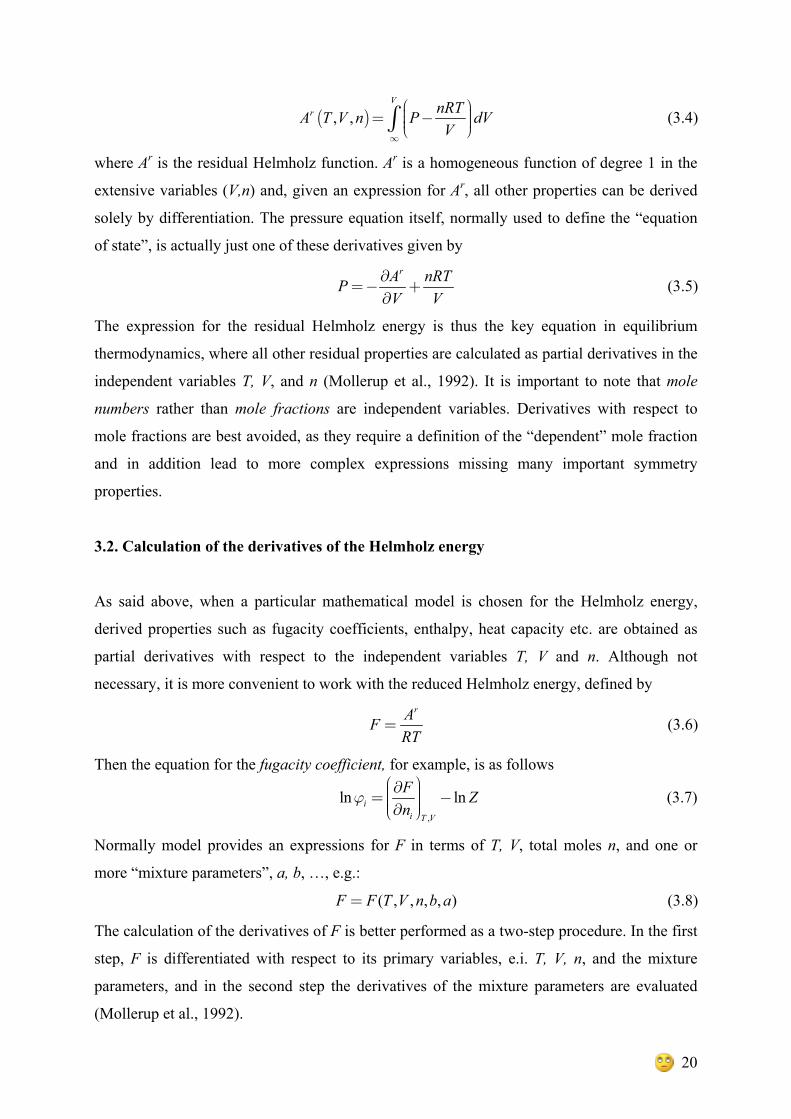
20

( ), ,V

r nRTA T V n P dVV

∞

⎛ ⎞⎟⎜= − ⎟⎜ ⎟⎜⎝ ⎠∫ (3.4)

where Ar is the residual Helmholz function. Ar is a homogeneous function of degree 1 in the

extensive variables (V,n) and, given an expression for Ar, all other properties can be derived

solely by differentiation. The pressure equation itself, normally used to define the “equation

of state”, is actually just one of these derivatives given by

rA nRTP

V V∂

=− +∂

(3.5)

The expression for the residual Helmholz energy is thus the key equation in equilibrium

thermodynamics, where all other residual properties are calculated as partial derivatives in the

independent variables T, V, and n (Mollerup et al., 1992). It is important to note that mole

numbers rather than mole fractions are independent variables. Derivatives with respect to

mole fractions are best avoided, as they require a definition of the “dependent” mole fraction

and in addition lead to more complex expressions missing many important symmetry

properties.

3.2. Calculation of the derivatives of the Helmholz energy

As said above, when a particular mathematical model is chosen for the Helmholz energy,

derived properties such as fugacity coefficients, enthalpy, heat capacity etc. are obtained as

partial derivatives with respect to the independent variables T, V and n. Although not

necessary, it is more convenient to work with the reduced Helmholz energy, defined by

rAF

RT= (3.6)

Then the equation for the fugacity coefficient, for example, is as follows

,

ln lnii T V

F Zn

ϕ⎛ ⎞∂ ⎟⎜ ⎟= −⎜ ⎟⎜ ⎟⎜∂⎝ ⎠

(3.7)

Normally model provides an expressions for F in terms of T, V, total moles n, and one or

more “mixture parameters”, a, b, …, e.g.:

( , , , , )F F T V n b a= (3.8)

The calculation of the derivatives of F is better performed as a two-step procedure. In the first

step, F is differentiated with respect to its primary variables, e.i. T, V, n, and the mixture

parameters, and in the second step the derivatives of the mixture parameters are evaluated

(Mollerup et al., 1992).

21

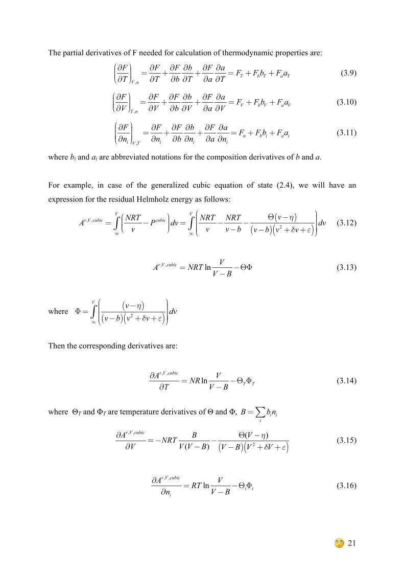
The partial derivatives of F needed for calculation of thermodynamic properties are:

,

T b T a TV n

F F F b F a F F b F aT T b T a T

⎛ ⎞∂ ∂ ∂ ∂ ∂ ∂⎟⎜ = + + = + +⎟⎜ ⎟⎜⎝ ⎠∂ ∂ ∂ ∂ ∂ ∂ (3.9)

,

V b V a VT n

F F F b F a F F b F aV V b V a V

⎛ ⎞∂ ∂ ∂ ∂ ∂ ∂⎟⎜ = + + = + +⎟⎜ ⎟⎜⎝ ⎠∂ ∂ ∂ ∂ ∂ ∂ (3.10)

,

n b i a ii i i iV T

F F F b F a F F b F an n b n a n

⎛ ⎞∂ ∂ ∂ ∂ ∂ ∂⎟⎜ ⎟ = + + = + +⎜ ⎟⎜ ⎟⎜∂ ∂ ∂ ∂ ∂ ∂⎝ ⎠ (3.11)

where bi and ai are abbreviated notations for the composition derivatives of b and a.

For example, in case of the generalized cubic equation of state (2.4), we will have an

expression for the residual Helmholz energy as follows:

( )

( )( ), ,

2

V Vr V cubic cubic vNRT NRT NRTA P dv dv

v v v b v b v vη

δ ε∞ ∞

⎛ ⎞⎛ ⎞ Θ − ⎟⎜ ⎟⎟⎜ ⎜= − = − − ⎟⎟⎜ ⎜ ⎟⎟⎜ ⎜⎝ ⎠ − ⎟− + + ⎟⎜⎝ ⎠∫ ∫ (3.12)

, , lnr V cubic VA NRTV B

= −ΘΦ−

(3.13)

where ( )

( )( )2

V vdv

v b v vη

δ ε∞

⎛ ⎞− ⎟⎜ ⎟⎜Φ= ⎟⎜ ⎟⎜ ⎟− + + ⎟⎜⎝ ⎠∫

Then the corresponding derivatives are:

, ,

lnr V cubic

T TA VNR

T V B∂

= −Θ Φ∂ −

(3.14)

where ΘT and ΦT are temperature derivatives of Θ and Φ, i i

i

B b n=∑

( )( )

, ,

2

( )( )

r V cubicA B VNRTV V V B V B V V

ηδ ε

∂ Θ −=− −

∂ − − + + (3.15)

, ,

lnr V cubic

i ii

A VRTn V B

∂= −ΘΦ

∂ − (3.16)

22

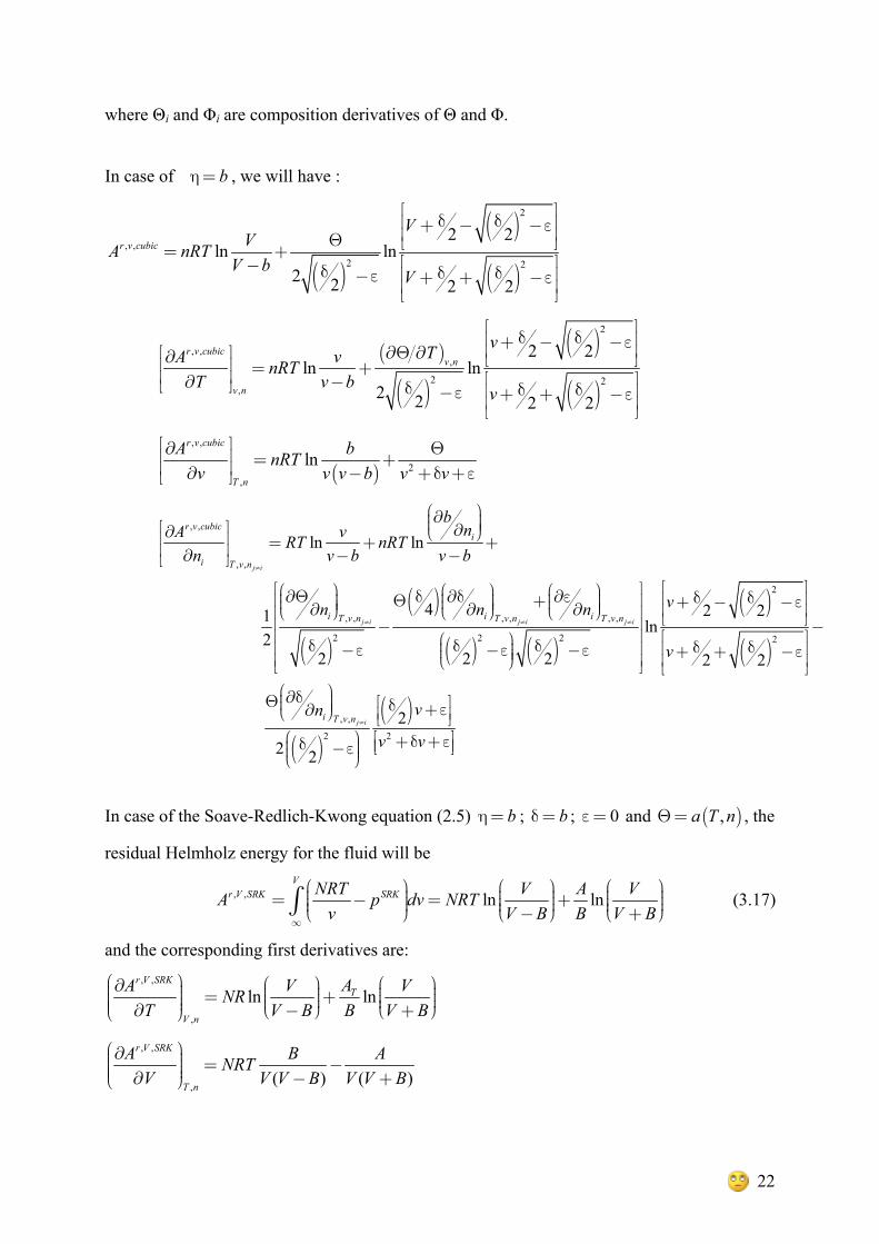
where Θi and Φi are composition derivatives of Θ and Φ.

In case of bη= , we will have :

( )

( )

( )

2

, ,

2 2

2 2ln ln

2 2 2 2

r v cubic

VVA nRT

V bV

⎡ ⎤δ δ⎢ ⎥+ − −ε⎢ ⎥Θ ⎣ ⎦= +⎡ ⎤− δ δ δ⎢ ⎥−ε + + −ε⎢ ⎥⎣ ⎦

( )

( )

( )

( )

2

, ,,

2 2,

2 2ln ln

2 2 2 2

r v cubicv n

v n

vTA vnRTT v b

v

⎡ ⎤δ δ⎢ ⎥+ − −ε⎢ ⎥∂Θ ∂⎡ ⎤∂ ⎣ ⎦⎢ ⎥ = +⎢ ⎥ ⎡ ⎤∂ −⎣ ⎦ δ δ δ⎢ ⎥−ε + + −ε⎢ ⎥⎣ ⎦

( )

, ,

2,

lnr v cubic

T n

A bnRTv v v b v v

⎡ ⎤∂ Θ⎢ ⎥ = +⎢ ⎥∂ − +δ +ε⎣ ⎦

( )

( )

( ) ( )

( )

, ,

, ,

2

, , , , , ,

2 2 2

ln ln

4 2 21 ln2

2 2 2 2

j i

j i j i j i

r v cubici

i T v n

i i iT v n T v n T v n

bnA vRT nRT

n v b v b

vn n n

v

≠

≠ ≠ ≠

⎛ ⎞∂ ⎟⎜ ⎟⎜⎡ ⎤ ⎟∂∂ ⎝ ⎠⎢ ⎥ = + +⎢ ⎥∂ − −⎣ ⎦

⎡ ⎤⎡ ⎤⎛ ⎞ ⎛ ⎞ ⎛ ⎞∂Θ δ ∂δ ∂ε δ δ⎟ ⎟ ⎟ ⎢ ⎥⎜ ⎜ ⎜Θ +⎢ ⎥ + − −ε⎟ ⎟ ⎟⎜ ⎜ ⎜⎟ ⎟ ⎟∂ ∂ ∂⎝ ⎠ ⎝ ⎠ ⎝ ⎠ ⎢ ⎥⎢ ⎥ ⎣ ⎦⎢ ⎥−⎢ ⎥⎛ ⎞δ δ δ δ⎟⎜⎢ ⎥−ε −ε −ε +⎟⎜ ⎟⎝ ⎠⎢ ⎥⎣ ⎦

( )

( )( )

2

, ,

2 2

2

2

2 2

j ii T v n

vn

v v≠

−⎡ ⎤δ⎢ ⎥+ −ε⎢ ⎥⎣ ⎦

⎛ ⎞∂δ ⎟⎜Θ ⎡ ⎤⎟ δ⎜ ⎟ +ε∂⎝ ⎠ ⎢ ⎥⎣ ⎦⎛ ⎞ ⎡ ⎤+δ +εδ ⎟ ⎢ ⎥⎜ −ε ⎣ ⎦⎟⎜ ⎟⎝ ⎠

In case of the Soave-Redlich-Kwong equation (2.5) bη= ; bδ = ; 0ε = and ( ),a T nΘ= , the

residual Helmholz energy for the fluid will be

, , ln lnV

r V SRK SRKNRT V A VA p dv NRTv V B B V B

∞

⎛ ⎞ ⎛ ⎞ ⎛ ⎞⎟ ⎟ ⎟⎜ ⎜ ⎜= − = +⎟ ⎟ ⎟⎜ ⎜ ⎜⎟ ⎟ ⎟⎜ ⎜ ⎜⎝ ⎠ ⎝ ⎠ ⎝ ⎠− +∫ (3.17)

and the corresponding first derivatives are: , ,

,

ln lnr V SRK

T

V n

AA V VNRT V B B V B

⎛ ⎞ ⎛ ⎞ ⎛ ⎞∂ ⎟⎜ ⎟ ⎟⎜ ⎜⎟ = +⎟ ⎟⎜ ⎜ ⎜⎟ ⎟ ⎟⎜ ⎜ ⎜⎟⎜ ⎝ ⎠ ⎝ ⎠∂ − +⎝ ⎠

, ,

, ( ) ( )

r V SRK

T n

A B ANRTV V V B V V B

⎛ ⎞∂ ⎟⎜ ⎟ = −⎜ ⎟⎜ ⎟⎜ ∂ − +⎝ ⎠

23

`

, ,

, ,

1ln ln( )

j k

r V SRKi i i

ii T V N

b Ab AbA V VRT NRT AN V B V B B B V B B V B

≠

⎛ ⎞ ⎛ ⎞⎛ ⎞ ⎛ ⎞∂ ⎟⎜ ⎟⎟ ⎟⎜⎜ ⎜⎟ = + + − −⎜ ⎟⎟ ⎟⎜⎜ ⎜⎟ ⎟⎟ ⎟⎜ ⎜ ⎜⎜⎟⎜ ⎝ ⎠ ⎝ ⎠⎝ ⎠∂ − − + +⎝ ⎠

where coefficients are defined as follows:

i ii

B b n=∑ (3.18)

( )1i j i j iji j

A a a n n k= −∑∑ (3.19)

2 (1 )i i j j iji ji

AA a a n kn

∂= = −

∂ ∑∑ (3.20)

24

4. THE CPA EQUATION OF STATE

Species forming hydrogen bonds often exhibit unusual thermodynamic behaviour. The strong

attractive interactions between molecules of the same species (self-association) or between

molecules of different species (cross-association). These interactions may strongly affect the

thermodynamic properties of the fluids. Thus, the chemical equilibria between clusters should

be taken into account in order to develop a reliable thermodynamic model.

The Cubic-Plus-Association (CPA) model is an equation of state that combines the cubic

SRK equation of state and an association (chemical) term described below. In terms of the

compressibility factor Z it has an appearance:

SRK assocZ Z Z= + | (4.1)

The compressibility factor contribution from the SRK equation of state is:

( )

( )SRK m

m m

V a TZV b RT V b

= −− +

(4.2)

and the contribution from the association term is given by:

1 12

i

i i

Aassoci i

i i A A i

XZ x

Xρ

ρ

⎡ ⎤⎛ ⎞∂⎟⎜⎢ ⎥⎟⎜= − ⎟⎢ ⎥⎜ ⎟⎜ ∂⎟⎢⎝ ⎠ ⎥⎣ ⎦∑ ∑ ∑ (4.3)

where Vm is the molar volume, iAX is the mole fraction of the molecule i not bonded at site A,

i.e. the monomer fraction, and xi is the superficial (apparent) mole fraction of component i.

The small letters i and j are used to index the molecules, and capital letters A and B are used

to index the bonding sites on a given molecule.

While the SRK model accounts for the physical interaction contribution between the species,

the association term in CPA takes into account the specific site-site interaction due to

hydrogen bonding. The association term employed in CPA is identical with the one used in

SAFT.

Before we describe the model, let’s give definitions of “sites” and “site-related” parameters

used in CPA and SAFT models.

25

4.1. Association energy and volume parameters

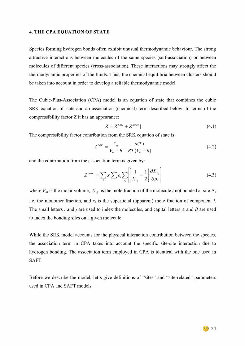
The key features of the hydrogen-bonds are their strength, short range, and high degree of

localization. In Fig. 4.1. it is shown a simple example of prototype spheres, or spherical

segments, with one associating site, A. Such spheres can only form an AA-bonded dimer

when both distance and orientation are favourable.

Fig. 4.1. Model of hard spheres with a single associating site A illustrating a simple case of molecular association due to short-distance, highly orientational, site-site attraction (Chapman et al., 1990)

The associating bond strength is quantified by a square-well potential, which, in turn, is

characterized by two parameters. The parameter εAA characterizes the association energy (well

depth), and the parameter κAA characterizes the association volume (corresponds to the well

width rAA). In general, the number of association sites on a single molecule is not constrained

and they are labelled with capital letters A, B, C, etc. Each association site is assumed to have

a different interaction with the various sites on another molecule. Examples of two associating

sites molecules are given in the Fig. 4.2.

Thus, for each pure component we need three molecular parameters, σ, ε/k, and m, which are

the temperature independent segment diameter in angstroms, the Lennard-Jones interaction

energy in Kelvins, and the number of segments per chain molecule, respectively. In addition

we need two association parameters, association energy, εAiBj/k in Kelvins and volume κAiBj

rAA

A A Wrong distance

AA Wrong orientation

A A Site-site attraction

σ

0

εAA

εAA Interaction energy κAA Interaction volume corresponding to rAA

26

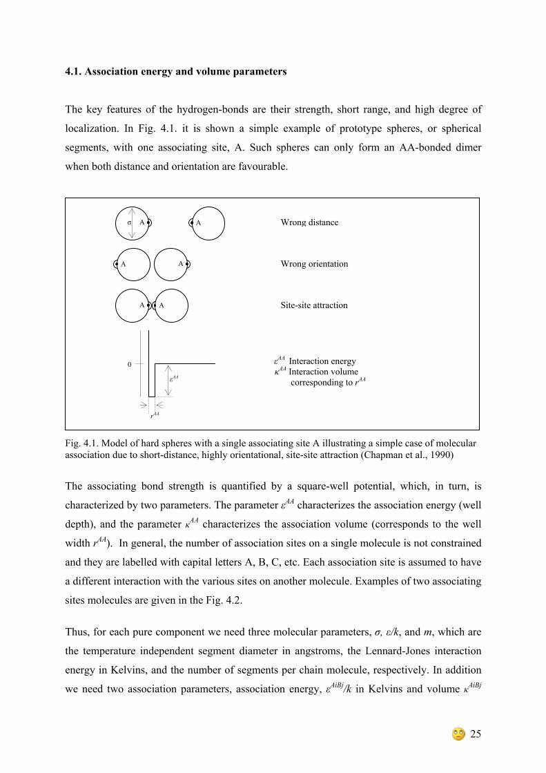
(dimensionless), for each site-site interaction. The usual method for deriving the σ, ε and m

values is to fit vapor pressure and density data for pure components. The association

parameters εAiBj/k and κAiBj can be fitted to bulk phase equilibrium data.

Fig. 4.2. Models of hard sphere (monomer) and chain (m-mer) molecules with two associating sites A

and B; the chain molecule represent nonspherical molecule (Chapman et al., 1990).

4.2. Association term in CPA EoS

For pure components, the association term is defined in terms of the residual Helmholz

energy ar per mole, defined as

( , , ) ( , , ) ( , , )r iga T V n a T V n a T V n= − (4.4)

where a and aig are the total Helmholz energy per mole and the ideal gas Helmholz energy per

mole at the same temperature and density. The residual Helmholz energy is a sum of three

terms representing contributions from different intermolecular forces: segment-segment

interaction, covalent chain-forming bonds, and site-site specific interactions among the

segments, for example, hydrogen-bonding interactions:

r seg chain assoca a a a= + + (4.5)

The extension of the CPA EoS to mixtures requires mixing rules only for the parameters of

the SRK-part, while the extension of the association term to mixtures is straightforward. The

mixing and combining rules for a and b are the classical van der Waals (Chapter 2.2.2).

The mixture Helmholz energy for the association term is linear with respect to mole fractions,

ni:

1 1ln2 2i i

i

assoc

i A Ai A

A n X XRT

⎛ ⎞⎟⎜= − + ⎟⎜ ⎟⎜⎝ ⎠∑ ∑ (4.6)

A

B

A

B 1 2 3 m

Model monomer (methanol)

Model m-mer (alkanol)

27

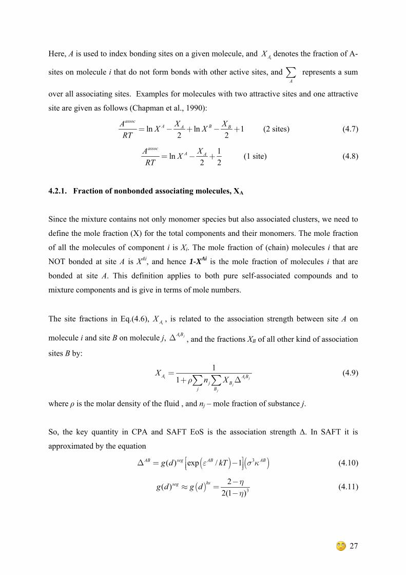
Here, A is used to index bonding sites on a given molecule, and iAX denotes the fraction of A-

sites on molecule i that do not form bonds with other active sites, and A∑ represents a sum

over all associating sites. Examples for molecules with two attractive sites and one attractive

site are given as follows (Chapman et al., 1990):

ln ln 12 2

assocA BA BX XA X X

RT= − + − + (2 sites) (4.7)

1ln2 2

assocA AXA X

RT= − + (1 site) (4.8)

4.2.1. Fraction of nonbonded associating molecules, XA

Since the mixture contains not only monomer species but also associated clusters, we need to

define the mole fraction (X) for the total components and their monomers. The mole fraction

of all the molecules of component i is Xi. The mole fraction of (chain) molecules i that are

NOT bonded at site A is XAi, and hence 1-XAi is the mole fraction of molecules i that are

bonded at site A. This definition applies to both pure self-associated compounds and to

mixture components and is give in terms of mole numbers.

The site fractions in Eq.(4.6), iAX , is related to the association strength between site A on

molecule i and site B on molecule j, i jA BΔ , and the fractions XB of all other kind of association

sites B by:

11i i j

j

j

A A Bj B

j B

Xn Xρ

=+ Δ∑ ∑

(4.9)

where ρ is the molar density of the fluid , and nj – mole fraction of substance j.

So, the key quantity in CPA and SAFT EoS is the association strength Δ. In SAFT it is

approximated by the equation

( ) ( )3( ) exp / 1AB seg AB ABg d kTε σ κ⎡ ⎤Δ = −⎢ ⎥⎣ ⎦ (4.10)

( ) 3

2( )2(1 )

hssegg d g d ηη

−≈ =

− (4.11)

28

Since CPA is a molecular based (not a segment-based) EoS, Kontogeorgis et al. (1996)

proposed to calculate the reduced fluid density by

4bV

η= (4.12)

where 32 / 3AVb N dπ= , and substituted the product 3 ABσ κ in Eq. (4.10) by equivalent bβ. So,

in CPA, i jA BΔ , the association (binding) strength between site A on molecule i and site B on

molecule j is given by:

( ) exp 1i j

i j i j

A BA B A Bref

ijg bRTε

ρ β⎡ ⎤⎛ ⎞⎟⎜⎢ ⎥⎟Δ = −⎜ ⎟⎢ ⎥⎜ ⎟⎟⎜⎝ ⎠⎢ ⎥⎣ ⎦

(4.13)

where i jA Bε and i jA Bβ are the association energy and volume of interaction between site A of

molecule i and site B of molecule j, respectively, and ( )refg ρ is the radial distribution

function for the reference fluid.

The hard-sphere radial distribution is further simplified by Kontogeorgis et al.(1999) to:

1( )1 1.9

g ρη

=−

(4.14)

14

bη ρ=

Also Yakoumis et al.(2001) proposed a much simpler general expression for the association

term instead of Eq.(4.3):

( )1 ln1 12 i

i

associ A

i A

gZ n Xρρ

⎛ ⎞∂ ⎟⎜=− + ⎟ −⎜ ⎟⎜ ⎟⎜ ∂⎝ ⎠∑ ∑ (4.15)

where ( )( )( )( )2

1ln 1.91 1.9ln 41 1.9 1 1 1.9 1.94 1 1.9

bg b−

⎛ ⎞⎟⎜∂ ⎟⎜ ⎟⎜ ⎟ ⎛ ⎞− η∂ ⎝ ⎠ ⎟⎜= = − η − − η − =⎟⎜ ⎟⎜⎝ ⎠∂ρ ∂ρ − η

ln 1.91 1.9

g∂ ηρ =

∂ρ − η.

In term of Volume, we have the result for sCPA and CPA, respectively:

ln 0.4750.475

g BV B

∂ρ =

∂ρ −

(4.16)

29

ln (10 )2(8 )(4 )

g V BBV B V B

∂ −ρ =

∂ρ − − (4.17)

The resulting EoS is referred to as simplified CPA (sCPA).

All phase equilibria calculations performed in this work are based on the simplified CPA

model.

4.2.2. Association schemes

As seen from Eq. (4.15), the contribution of the association compressibility factor in CPA

depends on the choice of association scheme, i.e. number and type of association sites for the

associating compound.

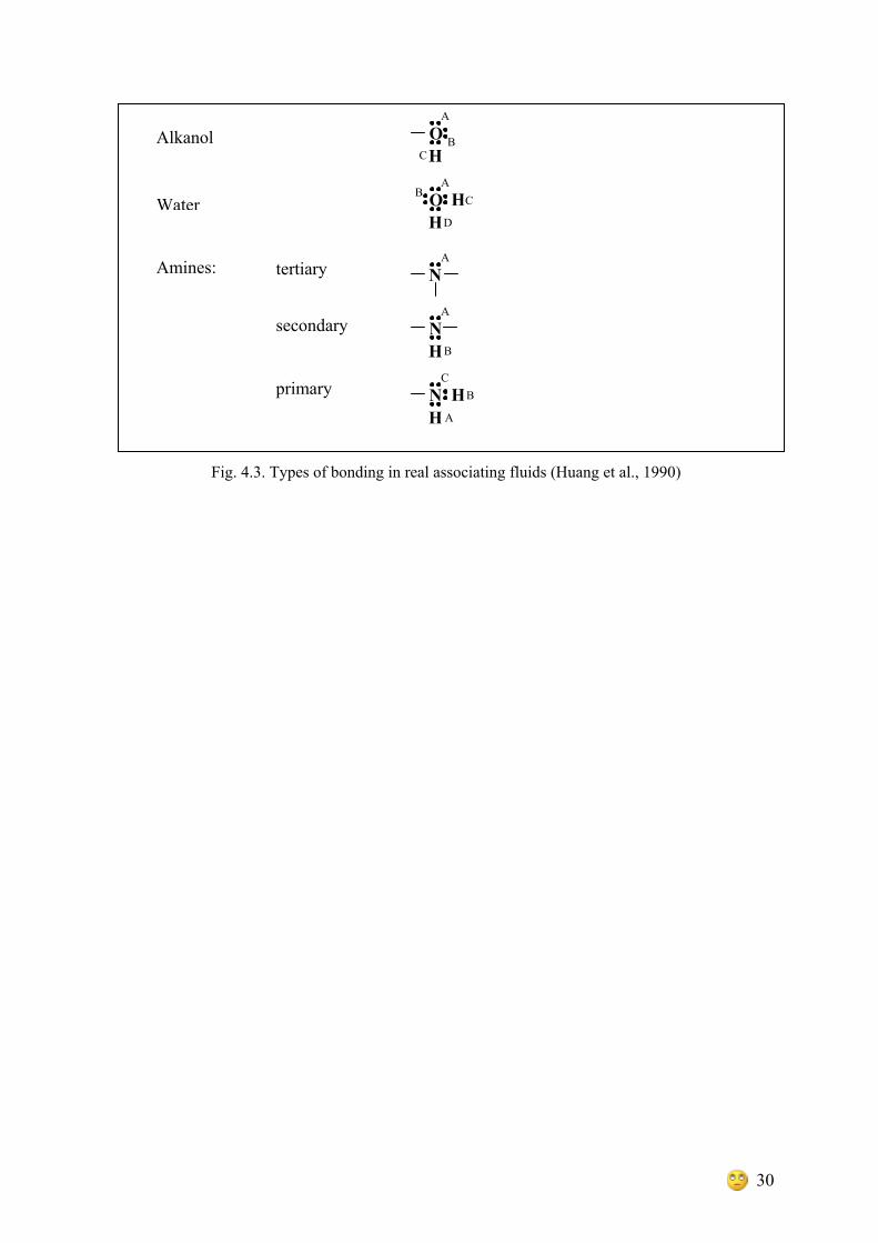
Huang and Radosz (1990) have classified eight different association schemes, which can be

applied to different molecules depending on the number and type of associating sites.

Examples of one-, two-, three-, and four-site molecules for real associating fluids are given in

Fig. 4.3. According to them, for example, for alkanols, each hydroxylic group (OH) has three

association sites, labelled A, B on oxygen and C on hydrogen. The association strength Δ due

to the like, oxygen-oxygen or hydrogen-hydrogen (AA, AB, BB, CC) interactions is assumed

to be equal to zero (since two lone pairs electrons on protons cannot attract each other). The

attraction can only occur between a lone pair electron and proton, i.e. the only non-zero Δ is

due to the unlike (AC and BC) interactions, which moreover are considered to be equivalent.

Another approximation is to allow only one site of oxygen (A) and one site of hydrogen (B).

In case of self association, the association scheme for alkanols is 2B.

30

Fig. 4.3. Types of bonding in real associating fluids (Huang et al., 1990)

N

C

OA

BH

Alkanol

Water COA

B

HD

H

Amines: A

A

NC

B

HH

NA

BH

tertiary

secondary

primary

31

The 2B association scheme (Huang et al., 1990):

00

AA BB

AB

Δ =Δ =

Δ ≠ (4.18)

1 1 4

2

AB

A B ABX Xρ

ρ− + + Δ

= =Δ

(4.19)

The 4C association scheme is used for water:

00

AA AB BB CC CD DD

AC AD BC BD

Δ =Δ =Δ =Δ =Δ =Δ =

Δ =Δ =Δ =Δ ≠ (4.20)

1 1 8

4

AC

A B C D ACX X X Xρ

ρ− + + Δ

= = = =Δ

(4.21)

These schemes are in agreement with the accepted physical picture that alcohols form linear

oligomers and water three-dimensional structures.

When CPA is used for the cross-associating mixture, e.g. alcohols-water, combining rules are

needed for the cross-association energy and volume parameters (ε AiBj, β AiBj) or for the

association strength ΔAiBj. Examples for the selection of the combining rule are given by Fu

and Sandler (1995). According to them, in water-alcohol mixture, water has three association

sites and an alcohol has two, but only the unbonded electron pair can form a hydrogen bond

with a hydrogen atom thereafter Eq. (4.22) can be described to all sites in methanol-water

system:

The scheme of self association : A1B1, A2C2 , B2C2 and the scheme of cross association

A1C2 , A2B1 , B2B1 (Kraska,1998) then we rewrite Eq. (4.9) as:

1 1 1 1 2

1 21 2

11 ( )A A B A C

B C

Xn X n X

=+ρ Δ + Δ

1 1 1 1 2 1 2

1 2 21 2 2

11 ( )B A B B B B A

A B A

Xn X n X n X

=+ρ Δ + Δ + Δ

2 2 2 2 2 2 1

2 2 12 2 1

11 ( )C C A C B C A

A B A

Xn X n X n X

=+ρ Δ + Δ + Δ

A

H O AB H

O A

B

H Alkanol (1) Water (2)

C

C D

32

2 2 2 2 1

2 12 1

11 ( )B B C B B

C B

Xn X n X

=+ρ Δ + Δ

2 2 2 2 1

2 12 1

11 ( )A A C A B

C B

Xn X n X

=+ρ Δ + Δ

If we set 2 2 2 2A C B CΔ =Δ , 2 2A BX X= , we have:

1 1 1 1 2

1 21 2

11 ( )A A B A C

B C

Xn X n X

=+ρ Δ + Δ

1 1 1 1 2

1 21 2

11 ( 2 )B A B B A

A B

Xn X n X

=+ρ Δ + Δ

2 2 2 2 1

2 12 1

11 (2 )C C A C A

A A

Xn X n X

=+ρ Δ + Δ

2 2 2 2 2 1

2 12 1

11 ( )A B B C B B

C B

X Xn X n X

= =+ρ Δ + Δ

There are four non-linear equations with four variables and we can solve them

simultaneously using Newton-Raphson method with objective function (for all sites) :

11 1 0

i j

A ii

all sites

A A j BX j B

F X X n X⎛ ⎞ ⎛ ⎞⎟⎜ ⎟⎜⎟ ⎟⎜ ⎜= +ρ − ≈⎟ ⎟⎜ ⎜⎟ ⎟⎜ ⎟⎜⎟⎜ ⎝ ⎠⎝ ⎠∑ ∑ ∑

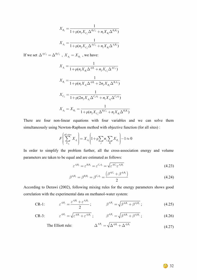
In order to simplify the problem further, all the cross-association energy and volume

parameters are taken to be equal and are estimated as follows:

1 2 1 2 1 2 1 1 2 2A B B B C A A C A Bε ε ε ε ε= = = (4.23)

( )1 1 2 2

1 2 1 2 1 2

2

A C A BA B B B C A

β ββ β β

+= = = (4.24)

According to Derawi (2002), following mixing rules for the energy parameters shows good

correlation with the experimental data on methanol-water system:

CR-1: 1 1 2 2

2i j

A B A BA B ε ε

ε+

= ; 1 1 2 2i jA B A B A Bβ β β= + ; (4.25)

CR-3: 1 1 2 2i jA B A B A Bε ε ε= + ; 1 1 2 2i jA B A B A Bβ β β= + ; (4.26)

The Elliott rule: 1 1 2 2i jA B A B A BΔ = Δ +Δ (4.27)

33

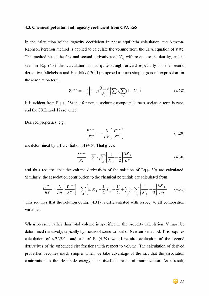
4.3. Chemical potential and fugacity coefficient from CPA EoS

In the calculation of the fugacity coefficient in phase equilibria calculation, the Newton-

Raphson iteration method is applied to calculate the volume from the CPA equation of state.

This method needs the first and second derivatives of iAX with respect to the density, and as

seen in Eq. (4.3) this calculation is not quite straightforward especially for the second

derivative. Michelsen and Hendriks ( 2001) proposed a much simpler general expression for

the association term:

( )1 ln1 12 i

i

associ A

i A

gZ x Xρρ

⎛ ⎞∂ ⎟⎜=− + ⎟ −⎜ ⎟⎜ ⎟⎜ ∂⎝ ⎠∑ ∑ (4.28)

It is evident from Eq. (4.28) that for non-associating compounds the association term is zero,

and the SRK model is retained.

Derived properties, e.g.

assoc assocP A

RT V RT⎛ ⎞∂ ⎟⎜ ⎟=− ⎜ ⎟⎜ ⎟⎜∂ ⎝ ⎠

(4.29)

are determined by differentiation of (4.6). That gives:

1 12

i

i i

assocA

ii A A

XP nRT X V

⎛ ⎞∂⎟⎜ ⎟⎜= − ⎟⎜ ⎟⎜ ∂⎟⎝ ⎠∑ ∑ (4.30)

and thus requires that the volume derivatives of the solution of Eq.(4.30) are calculated.

Similarly, the association contribution to the chemical potentials are calculated from

1 1 1 1ln2 2 2

j

i i

i j j

assoc assocAi

A A jA j Ai A i

XA X X nRT n RT X nμ ⎛ ⎞∂⎛ ⎞ ⎛ ⎞ ⎟∂ ⎜⎟⎜ ⎟⎟⎜ ⎜⎟= = − + + − ⎟⎟⎜ ⎜ ⎜⎟ ⎟⎟⎜ ⎜⎟⎜ ⎜⎝ ⎠∂ ∂⎟⎝ ⎠ ⎜⎝ ⎠

∑ ∑ ∑ (4.31)

This requires that the solution of Eq. (4.31) is differentiated with respect to all composition

variables.

When pressure rather than total volume is specified in the property calculation, V must be

determined iteratively, typically by means of some variant of Newton’s method. This requires

calculation of /P V∂ ∂ , and use of Eq.(4.29) would require evaluation of the second

derivatives of the unbonded site fractions with respect to volume. The calculation of derived

properties becomes much simpler when we take advantage of the fact that the association

contribution to the Helmholz energy is in itself the result of minimization. As a result,

34

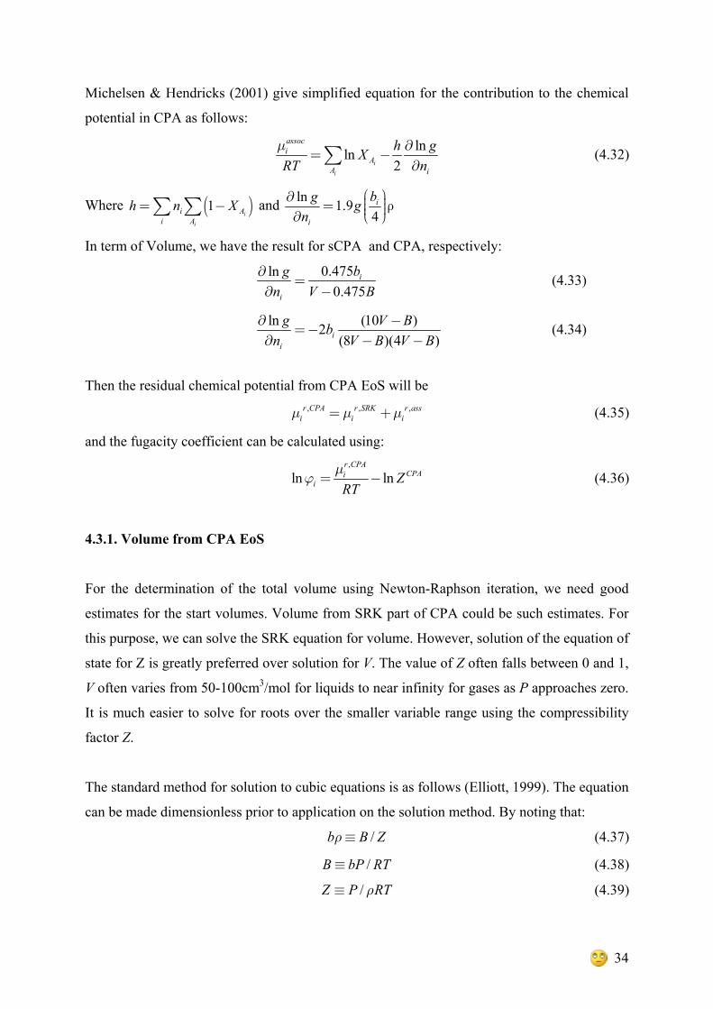
Michelsen & Hendricks (2001) give simplified equation for the contribution to the chemical

potential in CPA as follows:

lnln2i

i

associ

AA i

h gXRT nμ ∂

= −∂∑ (4.32)

Where ( )1i

i

i Ai A

h n X= −∑ ∑ and ln 1.94

i

i

bg gn

⎛ ⎞∂ ⎟⎜= ρ⎟⎜ ⎟⎜⎝ ⎠∂

In term of Volume, we have the result for sCPA and CPA, respectively:

0.475ln0.475

i

i

bgn V B

∂=

∂ − (4.33)

ln (10 )2(8 )(4 )i

i

g V Bbn V B V B

∂ −=−

∂ − − (4.34)

Then the residual chemical potential from CPA EoS will be

, , ,r CPA r SRK r assi i iμ μ μ= + (4.35)

and the fugacity coefficient can be calculated using:

,

ln lnr CPA

CPAii Z

RTμ

ϕ = − (4.36)

4.3.1. Volume from CPA EoS

For the determination of the total volume using Newton-Raphson iteration, we need good

estimates for the start volumes. Volume from SRK part of CPA could be such estimates. For

this purpose, we can solve the SRK equation for volume. However, solution of the equation of

state for Z is greatly preferred over solution for V. The value of Z often falls between 0 and 1,

V often varies from 50-100cm3/mol for liquids to near infinity for gases as P approaches zero.

It is much easier to solve for roots over the smaller variable range using the compressibility

factor Z.

The standard method for solution to cubic equations is as follows (Elliott, 1999). The equation

can be made dimensionless prior to application on the solution method. By noting that:

/b B Zρ≡ (4.37)

/B bP RT≡ (4.38)

/Z P RTρ≡ (4.39)

35

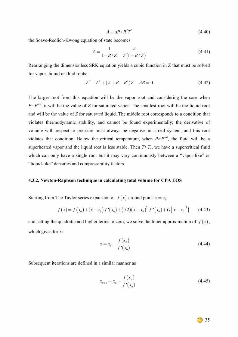
2 2/A aP R T≡ (4.40)

the Soave-Redlich-Kwong equation of state becomes

( )

11 / 1 /

AZB Z Z B Z

= −− +

(4.41)

Rearranging the dimensionless SRK equation yields a cubic function in Z that must be solved

for vapor, liquid or fluid roots:

3 2 2( ) 0Z Z A B B Z AB− + + − − = (4.42)

The larger root from this equation will be the vapor root and considering the case when

P=Psat, it will be the value of Z for saturated vapor. The smallest root will be the liquid root

and will be the value of Z for saturated liquid. The middle root corresponds to a condition that

violates thermodynamic stability, and cannot be found experimentally; the derivative of

volume with respect to pressure must always be negative in a real system, and this root

violates that condition. Below the critical temperature, when P>Psat, the fluid will be a

superheated vapor and the liquid root is less stable. Then T>Tc, we have a supercritical fluid

which can only have a single root but it may vary continuously between a “vapor-like” or

“liquid-like” densities and compressibility factors.

4.3.2. Newton-Raphson technique in calculating total volume for CPA EOS

Starting from The Taylor series expansion of ( )f x around point 0x x= :

( ) ( ) ( ) ( ) ( )( ) ( ) ( )2 30 0 0 0 0 0' 1 2 ''f x f x x x f x x x f x O x x= + − + − + − (4.43)

and setting the quadratic and higher terms to zero, we solve the linier approximation of ( )f x ,

which gives for x:

( )( )

00

0'f x

x xf x

= − (4.44)

Subsequent iterations are defined in a similar manner as

( )( )1 '

nn n

n

f xx x

f x+ = − (4.45)

36

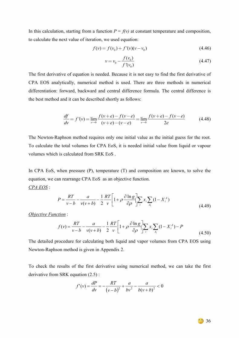
In this calculation, starting from a function P = f(v) at constant temperature and composition,

to calculate the next value of iteration, we used equation:

0 0( ) ( ) '( )( )f v f v f v v v= + − (4.46)

00

0

( )'( )

f vv vf v

= − (4.47)

The first derivative of equation is needed. Because it is not easy to find the first derivative of

CPA EOS analytically, numerical method is used. There are three methods in numerical

differentiation: forward, backward and central difference formula. The central difference is

the best method and it can be described shortly as follows:

0 0

( ) ( ) ( ) ( )'( ) lim lim( ) ( ) 2e e

df f v e f v e f v e f v ef vdv v e v e e→ →

+ − − + − −= = =

+ − − (4.48)

The Newton-Raphson method requires only one initial value as the initial guess for the root.

To calculate the total volumes for CPA EoS, it is needed initial value from liquid or vapour

volumes which is calculated from SRK EoS .

In CPA EoS, when pressure (P), temperature (T) and composition are known, to solve the

equation, we can rearrange CPA EoS as an objective function.

CPA EOS :

)1(ln121

)( ∑∑ −⎥⎦

⎤⎢⎣

⎡∂∂

+−+

−−

=iA

Ai

ii Xxg

vRT

bvva

bvRTP

ρρ

(4.49)

Objective Function :

PXxgv

RTbvv

abv

RTvfiA

Ai

ii −−⎥

⎦

⎤⎢⎣

⎡∂∂

+−+

−−

= ∑∑ )1(ln121

)()(

ρρ

(4.50)

The detailed procedure for calculating both liquid and vapor volumes from CPA EOS using

Newton-Raphson method is given in Appendix 2.

To check the results of the first derivative using numerical method, we can take the first

derivative from SRK equation (2.5) :

( )0

)()(' 222 <

+−+

−−==

bvba

bva

bvRT

dvdPvf

37

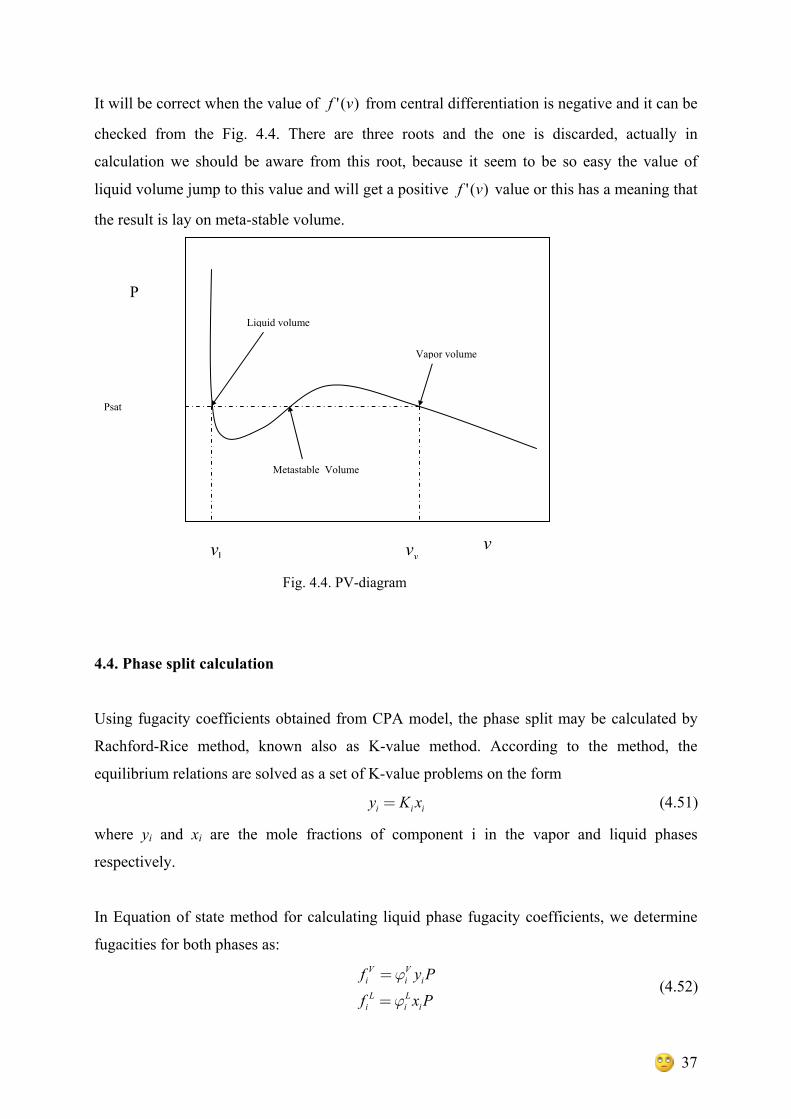
It will be correct when the value of )(' vf from central differentiation is negative and it can be

checked from the Fig. 4.4. There are three roots and the one is discarded, actually in

calculation we should be aware from this root, because it seem to be so easy the value of

liquid volume jump to this value and will get a positive )(' vf value or this has a meaning that

the result is lay on meta-stable volume.

Fig. 4.4. PV-diagram

4.4. Phase split calculation

Using fugacity coefficients obtained from CPA model, the phase split may be calculated by

Rachford-Rice method, known also as K-value method. According to the method, the

equilibrium relations are solved as a set of K-value problems on the form

i i iy K x= (4.51)

where yi and xi are the mole fractions of component i in the vapor and liquid phases

respectively.

In Equation of state method for calculating liquid phase fugacity coefficients, we determine

fugacities for both phases as:

V V

i i iL L

i i i

f y P

f x P

ϕ

ϕ

=

= (4.52)

Vapor volume

Liquid volume

v

P

Metastable Volume

vvlv

Psat

38

Then, using the condition for thermodynamic phase equilibrium(1.11), we can write:

Li

i Vi

K ϕϕ

= (4.53)

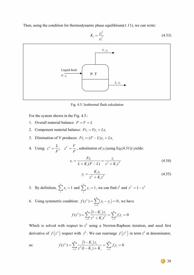
Fig. 4.5. Isothermal flash calculation

For the system shown in the Fig. 4.5.:

1. Overall material balance: F V L= +

2. Component material balance: i i iFz Vy Lx= +

3. Elimination of V produces: ( )i i iFz F L y Lx= − +

4. Using: ;L LzF

= V VzF

= , substitution of yi (using Eq.(4.51)) yields:

( )i i

i L Vi i

Fz zxL K F L z K z

= =+ − +

(4.54)

i ii L V

i

K zyz K z

=+

(4.55)

5. By definition, 1

1n

ix =∑ and 1

1n

iy =∑ , we can find zL and 1V Lz z= −

6. Using symmetric condition: ( )1

( ) 0n

Li i

i

f z x y=

= − =∑ , we have

( )1 1

1( ) 0

n ni iL

i iL Vi ii

K zf z f z

z K z= =

−= = =

+∑ ∑

Which is solved with respect to zL using a Newton-Raphson iteration, and need first

derivative of ( )Lf z respect with zL.. We can rearrange ( )Lf z in term zL at denominator,

as: ( )

1 1

1( ) 0

(1 )

n ni iL

i iLi ii i

K zf z f z

z K K= =

−= = =

− +∑ ∑

Liquid feed:

F, zi

L, xi

V, yi

P, T

39

( )

( )

22

21 1

1( ) '( )(1 )L

L n ni iL

i iLi ii

K zf z f z f zz z K K= =

−∂= =− =−

∂ − +∑ ∑

11

, 1 , , 2

1

nL k L k L k

i iLi

fz z f z f z fz

−−+

=

⎛ ⎞⎛ ⎞∂ ⎟⎜⎟⎜= − = + ⎟⎟ ⎜⎜ ⎟⎟⎜ ⎜ ⎟⎝ ⎠∂ ⎝ ⎠∑ (4.56)

Substitution of the obtained zL into Eqs. (4.54) and (4.55) produce new values of xi and yi.

4.4.1. Bubble-Point Pressure Calculation

Starting from Eq (1.11) and (4.52), we can write : L V Vi i i i ix P y P=ϕ ϕ (4.57)

The relation between iϕ and the residual chemical potential of component i can be found

from Eq (1.25),. Then the phase equilibrium constant, Ki can be obtained from Eq (4.53),

which can be rewritten as follows:

expL Vres res

v i ii

L

ZKZ RT RT

⎡ ⎤⎛ ⎞ ⎛ ⎞⎢ ⎥⎟ ⎟⎜ ⎜⎟ ⎟= −⎜ ⎜⎢ ⎥⎟ ⎟⎜ ⎜⎟ ⎟⎜ ⎜⎝ ⎠ ⎝ ⎠⎢ ⎥⎣ ⎦

μ μ (4.58)

In Bubble-Point Pressure calculation we calculate vapour phase fraction of each component

until the sum of vapour phase fractions is equal to 1 (less than tolerance).

1i

C C

i ii i

y K x= =∑ ∑

4.5. Results and discussion

Vapor-liquid phase equilibria calculation has been performed for the binary cross-associating

mixture of methanol and water. The algorithm for the Matlab code is given in Appendix 1.

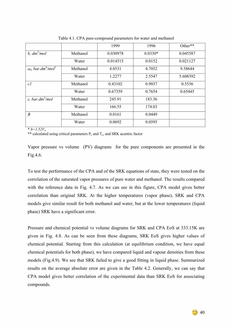
The CPA pure-compound parameters, used for the calculations, have been obtained by

Kontogeorgis et al. (1999), and are listed in the Table 4.1.

40

Table 4.1. CPA pure-compound parameters for water and methanol

1999 1996 Other**

Methanol 0.030978 0.0330* 0.045587 b, dm3/mol

Water 0.014515 0.0152 0.021127

Methanol 4.0531 4.7052 9.58644 a0, bar.dm6/mol2

Water 1.2277 2.5547 5.608392

Methanol 0.43102 0.9037 0.5536 c1

Water 0.67359 0.7654 0.65445

Methanol 245.91 183.36 ε, bar.dm3/mol

Water 166.55 174.03

Methanol 0.0161 0.0449 Β

Water 0.0692 0.0595

* b=1.52Vw ** calculated using critical parameters Pc and Tc, and SRK acentric factor

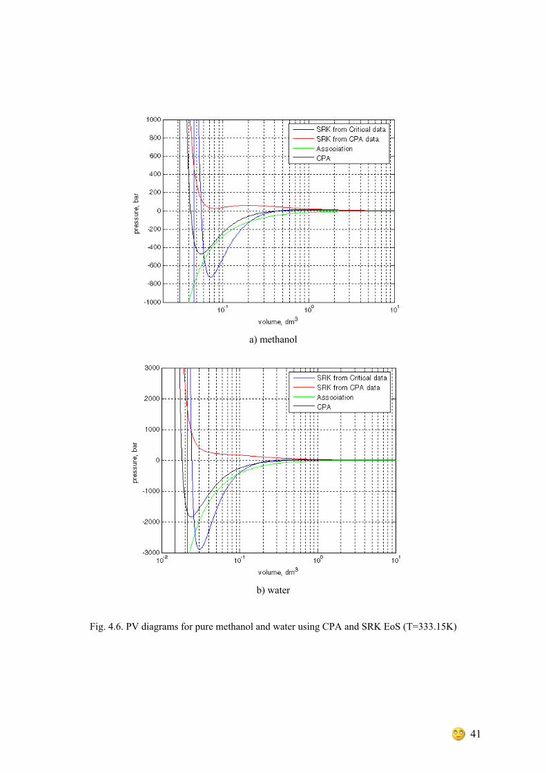
Vapor pressure vs volume (PV) diagrams for the pure components are presented in the

Fig.4.6.

To test the performance of the CPA and of the SRK equations of state, they were tested on the

correlation of the saturated vapor pressures of pure water and methanol. The results compared

with the reference data in Fig. 4.7. As we can see in this figure, CPA model gives better

correlation than original SRK. At the higher temperatures (vapor phase), SRK and CPA

models give similar result for both methanol and water, but at the lower temperatures (liquid

phase) SRK have a significant error.

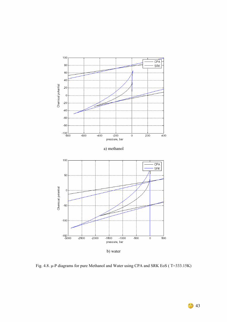
Pressure and chemical potential vs volume diagrams for SRK and CPA EoS at 333.15K are

given in Fig. 4.8. As can be seen from these diagrams, SRK EoS gives higher values of

chemical potential. Starting from this calculation (at equilibrium condition, we have equal

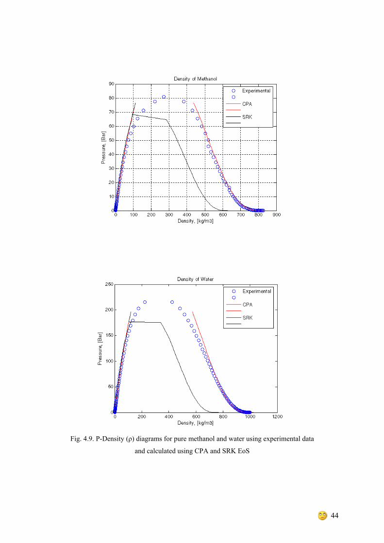
chemical potentials for both phase), we have compared liquid and vapour densities from these

models (Fig.4.9). We see that SRK failed to give a good fitting in liquid phase. Summarized

results on the average absolute error are given in the Table 4.2. Generally, we can say that

CPA model gives better correlation of the experimental data than SRK EoS for associating

compounds.

41

a) methanol

b) water

Fig. 4.6. PV diagrams for pure methanol and water using CPA and SRK EoS (T=333.15K)

42

Fig. 4.7. P-T diagrams for pure water and methanol using experimental data

and calculated using SRK and original CPA equations of state

Table 4.2. Average error calculated from SRK and CPA Model

SRK CPA Average Error (%)

Methanol Water Methanol Water

Saturated Pressure 6.09 6.73 1.11 7.07

Liquid Density 28.56 29.97 2.77 2.57

Vapor Density 8.96 10.19 8.88 9.03

43

a) methanol

b) water

Fig. 4.8. μ-P diagrams for pure Methanol and Water using CPA and SRK EoS ( T=333.15K)

44

Fig. 4.9. P-Density (ρ) diagrams for pure methanol and water using experimental data

and calculated using CPA and SRK EoS

45

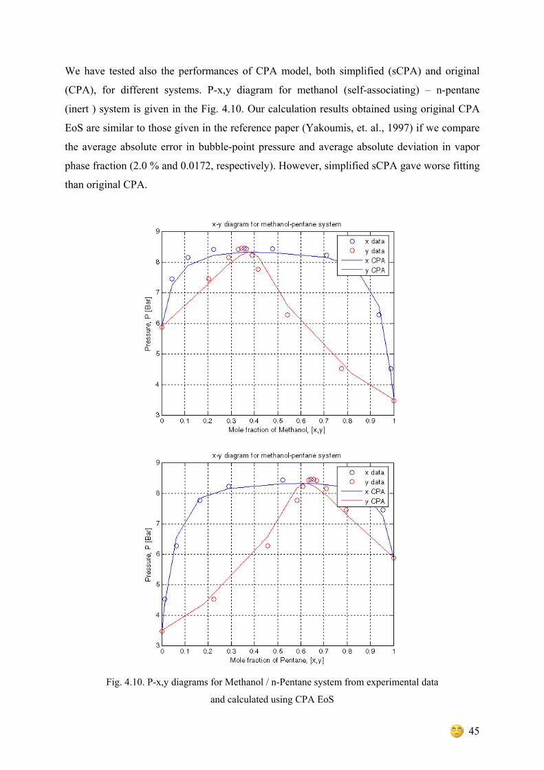
We have tested also the performances of CPA model, both simplified (sCPA) and original

(CPA), for different systems. P-x,y diagram for methanol (self-associating) – n-pentane

(inert ) system is given in the Fig. 4.10. Our calculation results obtained using original CPA

EoS are similar to those given in the reference paper (Yakoumis, et. al., 1997) if we compare

the average absolute error in bubble-point pressure and average absolute deviation in vapor

phase fraction (2.0 % and 0.0172, respectively). However, simplified sCPA gave worse fitting

than original CPA.

Fig. 4.10. P-x,y diagrams for Methanol / n-Pentane system from experimental data

and calculated using CPA EoS

46

P-x,y diagram for the methanol-water system is given in the Fig.4.11. This diagram is

obtained using simplified CPA EoS not taking into account the cross-association (two self-

associating compounds). The average error in bubble-point pressure calculation in this case is

9.48 % and the average absolute deviation in vapor phase fraction is 0.021. We used 2B

model for Methanol and 4C model for water.

Fig. 4.11. P-xy diagrams for methanol -Water system experimental data

and calculated using CPA EoS

47

As a result of our work, we have good correlation for pure components (methanol and water)

and system consisting of one self-associating and one inert compound (methanol – pentane).

The correlation of the experimental data for the methanol-water system was not that good,

because we did not take into account cross-association that takes place between methanol and

water molecules. We have tried to implement cross-association using schemes proposed by

Kraska (1998) but did not get any better results. So, further study should be done on the

implementation of the cross-association into sCPA model, that should give better fitting of the

experimental data.

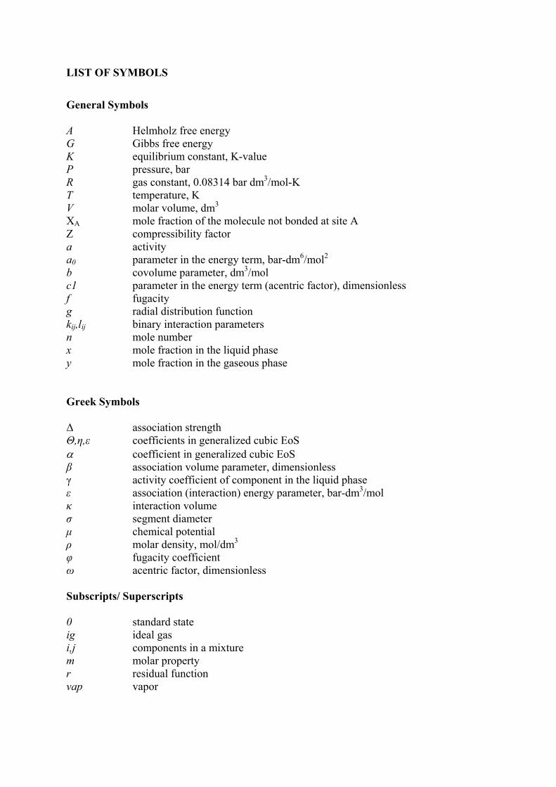
LIST OF SYMBOLS

General Symbols A Helmholz free energy G Gibbs free energy K equilibrium constant, K-value P pressure, bar R gas constant, 0.08314 bar dm3/mol-K T temperature, K V molar volume, dm3 XA mole fraction of the molecule not bonded at site A Z compressibility factor a activity a0 parameter in the energy term, bar-dm6/mol2

b covolume parameter, dm3/mol c1 parameter in the energy term (acentric factor), dimensionless f fugacity g radial distribution function kij,lij binary interaction parameters n mole number x mole fraction in the liquid phase y mole fraction in the gaseous phase Greek Symbols Δ association strength Θ,η,ε coefficients in generalized cubic EoS α coefficient in generalized cubic EoS β association volume parameter, dimensionless γ activity coefficient of component in the liquid phase ε association (interaction) energy parameter, bar-dm3/mol κ interaction volume σ segment diameter μ chemical potential ρ molar density, mol/dm3 φ fugacity coefficient ω acentric factor, dimensionless Subscripts/ Superscripts 0 standard state ig ideal gas i,j components in a mixture m molar property r residual function vap vapor

49

REFERENCES

Chapman W.G., Gubbins K.E., Jackson G., Radosz M., (1990), New reference equation of

state for associating liquids, Ind. Eng. Chem. Res., 29, 1709-1721

Derawi S.O., (2002), Modelling of phase equilibria containing associating fluids, Ph.D.

Thesis, Technical University of Denmark

Derawi S.O., Kontogeorgis G.M., Michelsen M.L., Stenby E.H., (2003), Extension of the

cubic-plus-association equation of state to glycol-water cross-associating systems, Ind.

Eng. Chem. Res., 42, 1470-1477

Derawi S.O., Michelsen M.L., Kontogeorgis G.M., Stenby E.H., (2003), Application of the

CPA equation of state to glycol/hydrocarbons liquid-liquid equilibria, Fluid Phase

Equilibria, 209, 163-184

Fu Y-H., Sandler S.I., (1995), A simplified SAFT equation of state for associating compounds

and mixtures, Ind. Eng. Chem. Res., 34, 1897-1909

Gao G.H., He Q.L., Yu Y.X., A simple equation of state for associating fluids

Ghosh P., (1999), Prediction of vapor-liquid equilibria using Peng-Robinson and Soave-

Redlich-Kwong equations of state, Chem. Eng. Technol., 22, 5, 379-399

Elliott J.R., Lira C.T., (1999), Introductory chemical engineering thermodynamics, Prentice

Hall PTR

Haug-Warberg, T., (2004), 45 Workouts in Thermodynamics, NTNU

Huang S.H., Radosz M., (1990), Equation of state for small, large, polydisperse, and

associating molecules, Ind. Eng. Chem. Res., 29, 2284-2294

Kent R.L., Eisenberg B., (1976), Better Data for Amine Treating, Hydrocarbon Processing, 2,

87-90

Kontogeorgis G.M., Voutsas E.C., Yakoumis I.V., Tassios D.P., (1996), An equation of state

for associating fluids, Ind. Eng. Chem. Res., 35, 4310-4318

Kraska T, (1998), Analytic and fast numerical solutions and approximations for Cross-

Association Models within SAFT, Ind. Eng. Chem. Res., 37, 4889-4892

Michelsen M.L., Hendriks E.M., (2001), Physical properties from association models, Fluid

Phase Equilibria, 180, 165-174

Mollerup J.M., Michelsen M.L., (1992), Calculation of thermodynamic equilibrium properties,

Fluid Phase Equilibria, 74, 1-15

Müller E.A., Gubbins K.E., (2001), Molecular-based equations of state for associating fluids:

a review of SAFT and related approaches

50

Nath A., Bender E., (1981), On the thermodynamics of associated solutions. II. Vapor-liquid

equilibria of binary systems with one associating component, Fluid Phase Equilibria, 7,

289-307

Polling B.E., Prausnitz J.M., O’Connell J.P., (2000), The properties of gases and liquids, 5th

ed., McGraw-Hill, NY

Redlich O., Kwong J.N.S., (1949), On the thermodynamics of solutions. 5. An equation of

state – fugacities of gaseous solutions, Chemical Reviews, 44, 1, 233-244

Sandler S.I. (edited by), (1993), Models for thermodynamic and phase equilibria calculations,

Marcel Dekker, NY

Soave G., (1972), Equilibrium constants from a modified Redlish-Kwong equation of state,

Chem. Eng. Sci., 27, 1197-1203

Solms N.von, Michelsen M.L., Kontogeorgis G.M., (2004), Applying association theories to

polar fluids, Ind. Eng. Chem. Res., 43, 1803-1806

Voutsas E.C., Kontogeorgis G.M., Yakoumis I.V., Tassios D.P., (1997), Correlation of liquid-

liquid equilibria for alcohol/hydrocarbon mixtures using the CPA equation of state,

Fluid Phase Equilibria, 132, 61-75

Voutsas E.C., Yakoumis I.V., Tassios D.P., (1999), Prediction of phase equilibria in water/

alcohol/alkane systems, Fluid Phase Equilibria, 158-160, 151-163

Yakoumis I.V., Kontogeorgis G.M., Voutsas E.C., Hendriks E.M., Tassios D.P., (1998),

Prediction of phase equilibria in binary aqueous systems containing alkanes,

cycloalkanes, and alkenes with the cubic-plus-association equation of state, Ind. Eng.

Chem. Res., 37, 4175-4182

Yakoumis I.V., Kontogeorgis G.M., Voutsas E.C., Tassios D.P., (1997), Vapor-liquid

equilibria for alcohol/hydrocarbon systems using the CPA equation of state, Fluid

Phase Equilibria, 130, 31-47

51

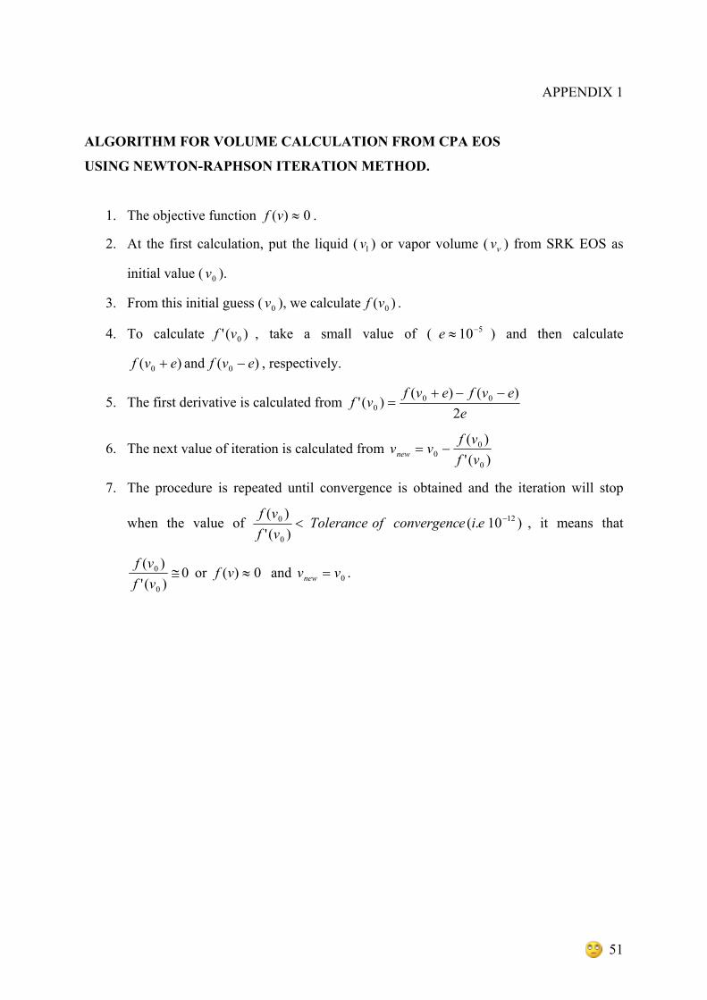
APPENDIX 1

ALGORITHM FOR VOLUME CALCULATION FROM CPA EOS

USING NEWTON-RAPHSON ITERATION METHOD.

1. The objective function 0)( ≈vf .

2. At the first calculation, put the liquid ( lv ) or vapor volume ( νv ) from SRK EOS as

initial value ( 0v ).

3. From this initial guess ( 0v ), we calculate )( 0vf .

4. To calculate )(' 0vf , take a small value of ( 510−≈e ) and then calculate

)( 0 evf + and )( 0 evf − , respectively.

5. The first derivative is calculated from e

evfevfvf

2)()(

)(' 000

−−+=

6. The next value of iteration is calculated from )(')(

0

00 vf

vfvvnew −=

7. The procedure is repeated until convergence is obtained and the iteration will stop

when the value of )10.()(')( 12

0

0 −< eieconvergencofTolerancevfvf

, it means that

0)(')(

0

0 ≅vfvf

or 0)( ≈vf and 0vvnew = .

52

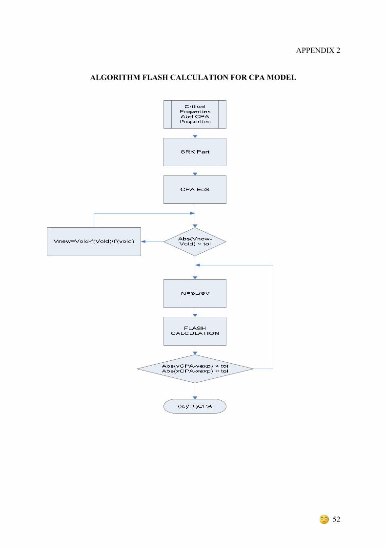
APPENDIX 2

ALGORITHM FLASH CALCULATION FOR CPA MODEL

53

ALGORITHM BUBBLE-POINT PRESSURE CALCULATION FOR CPA MODEL