This content has been downloaded from IOPscience. Please scroll down to see the full text.

Download details:

IP Address: 192.12.184.7

This content was downloaded on 11/03/2015 at 15:32

Please note that terms and conditions apply.

Calculation of grain boundary normals directly from 3D microstructure images

View the table of contents for this issue, or go to the journal homepage for more

2015 Modelling Simul. Mater. Sci. Eng. 23 035005

(http://iopscience.iop.org/0965-0393/23/3/035005)

Home Search Collections Journals About Contact us My IOPscience

Modelling and Simulation in Materials Science and Engineering

Modelling Simul. Mater. Sci. Eng. 23 (2015) 035005 (18pp) doi:10.1088/0965-0393/23/3/035005

Calculation of grain boundary normalsdirectly from 3D microstructure images

E J Lieberman1,2, A D Rollett1, R A Lebensohn2 andE M Kober3

1 Department of Materials Science and Engineering, Carnegie Mellon University,5000 Forbes Avenue, Pittsburgh, PA 15213, USA2 Materials Science and Technology Division, Los Alamos National Laboratory,MS G755, Los Alamos, NM 87455, USA3 Theoretical Division, Los Alamos National Laboratory, MS B214, Los Alamos,NM 87455, USA

E-mail: emk@lanl.gov

Received 10 October 2014, revised 17 January 2015Accepted for publication 10 February 2015Published 11 March 2015

AbstractThe determination of grain boundary normals is an integral part of thecharacterization of grain boundaries in polycrystalline materials. These normalvectors are difficult to quantify due to the discretized nature of availablemicrostructure characterization techniques. The most common method todetermine grain boundary normals is by generating a surface mesh from animage of the microstructure, but this process can be slow, and is subject tosmoothing issues. A new technique is proposed, utilizing first order Cartesianmoments of binary indicator functions, to determine grain boundary normalsdirectly from a voxelized microstructure image. To validate the accuracy of thistechnique, the surface normals obtained by the proposed method are comparedto those generated by a surface meshing algorithm. Specifically, the localdivergence between the surface normals obtained by different variants of theproposed technique and those generated from a surface mesh of a syntheticmicrostructure constructed using a marching cubes algorithm followed byLaplacian smoothing is quantified. Next, surface normals obtained with theproposed method from a measured 3D microstructure image of a Ni polycrystalare used to generate grain boundary character distributions (GBCD) for �3 and�9 boundaries, and compared to the GBCD generated using a surface meshobtained from the same image. The results show that the proposed technique isan efficient and accurate method to determine voxelized fields of grain boundarynormals.

Keywords: grain boundaries, microstructure, image analysis, moment analysis

(Some figures may appear in colour only in the online journal)

0965-0393/15/035005+18$33.00 © 2015 IOP Publishing Ltd Printed in the UK 1

Modelling Simul. Mater. Sci. Eng. 23 (2015) 035005 E J Lieberman et al

1. Introduction

Grain boundaries (GBs) are the interfaces between two disoriented crystals and, becausethey delimit changes in the orientation-dependent local properties of the solid, they haveconsiderable influence over the properties of polycrystalline materials. For example, manyforms of material failure, such as voids and cracks, tend to initiate and propagate alongGBs [1, 2]. The field of Grain Boundary Engineering has arisen to manipulate these interfacesto improve material properties [3, 4], and in order to do so full characterization of GBs isnecessary. GBs can be characterized at the mesoscale by five parameters. Three of theseparameters specify the misorientation, which is the transformation that brings the crystal latticesof the grains on either side of the boundary into coincidence. The other two specify the unitvector that is locally normal to the GB plane. These components are combined to produce afive-dimensional (5D) grain boundary character (GBC). The GBC is assumed to be sufficientto specify GB properties such as energy and mobility. The misorientation components of theGBC are rather easily calculated in terms of the orientation of neighboring points in space,which can be measured by techniques such as electron backscatter diffraction (EBSD). TheGB plane normals, however, are rather more difficult to acquire since they must be inferredfrom a set of points distributed in three dimensions. The GB plane normals are needed, forexample, to calculate the dihedral angles around triple junctions, which in turn are used tocalculate the GB energies and create grain boundary energy distributions [5, 6]. One methodof visually representing the GBC is to utilize grain boundary character distributions (GBCD),which is a stereographic projection of the interface orientations for a particular misorientationof interest [7, 8].

Some of the reasons as to why GB normals are difficult to obtain are explored here. First,as mentioned above, three-dimensional (3D) information is required and this is expensiveand time-consuming to acquire. The most common methods for getting 3D microstructureinformation are serial-sectioning combined with EBSD measurements, which is a destructivetechnique [9], and the recently introduced non-destructive high-energy diffraction microscopy(HEDM) [10]. Both methods result in a series of two-dimensional (2D) images that can thenbe aligned to form a 3D image. However, the GB normals are still not easily obtained fromthis stack of 2D images, due to the lack of information on the actual boundary inclination. Themicrostructure image obtained from EBSD or HEDM is similar to any other digital image;it consists of a grid of discrete points that does not explicitly include surfaces that would beneeded to provide information on GB topology. At best, boundaries are known to lie betweenneighboring sets of points that belong to two different grains as shown in figure 1. However,the details in between are not directly known.

Requiring actual 3D information can be avoided by using stereological methods to derivegeneral plane normal distributions [11, 12]. However, information on individual boundariescannot be obtained using stereology. Surface reconstruction, i.e. the method of generatingsurface information from a set of discrete points representing a shape, is required in orderto define the missing GB information in 3D data. This constitutes a difficult problem andmany different techniques have been proposed aiming at solving it. For example, Dey andGoswami [13] developed a technique for surface reconstruction utilizing intersecting Delaunayballs to determine the surfaces. Hoppe et al. [14] and Mitra and Nguyen [15] generated surfaceinformation by fitting tangent planes to some specified number of local points. A similarmethod was developed by Ivasishin [16] who combined it with a 3D Monte-Carlo model. Atechnique by Moore and Warren [17] utilized polynomial fitting to develop polyhedral surfaces.Among surface reconstruction techniques, the most common and widely accepted way ofapproximating the GB surfaces is to generate a surface mesh from voxelized microstructure

2

Modelling Simul. Mater. Sci. Eng. 23 (2015) 035005 E J Lieberman et al

Figure 1. An image for two grains, where each corner of the cubic grid of lines representsa measured orientation point in the material. If all eight vertices of the cube agree intheir orientation, the cube can be identified as belonging to that grain and is coloredappropriately. If the eight vertices are not all in agreement, the volume must be associatedwith the GB and is left transparent for this illustration.

images. Different variants of this methodology have been proposed. One of the most usedalgorithms for developing a surface mesh from image data is the ‘marching cubes’ method [18],which is used in many software programs including the one utilized in this work, known asDream.3D [19].

As with general surface reconstruction, the most common technique for GBcharacterization is based upon developing an explicit surface mesh. However, there arealso other methods that do not explicitly generate this mesh but still calculate surfaceinformation [7, 8, 20]. The methodology proposed by Ivasishin et al [16] is one of the few casesof GB normals calculated directly from 3D integer grid-based data. However, this techniquewas not validated against experimental microstructures. Another example of GB informationinferred from voxelized images is that of Chandross et al [21], who, however, focused onobtaining dihedral angles at triple lines.

In this work, we develop a new method based on the gradients of binary indicator fieldsdetermined from the voxelized image data. This is discussed in section 2. In section 3, wediscuss the validation of this technique first with synthetic microstructures and compare thesurface normals determined by the new technique with those calculated from a surface meshwith triangular elements, obtained using Dream.3D. Based on the analysis of these syntheticcases, the method is further utilized to obtain the GBCD of a pure nickel 3D microstructureimage obtained by HEDM. These results are compared to the GBCD previously determinedby Hefferan [22–24] for the same microstructure, but using a different surface reconstructiontechnique that instead utilizes the Computational Geometry Algorithms Library (CGAL)package. CGAL is software that is used to model surfaces for many applications ranging fromMaterials Science to Geology to Biology [25–27], to mention a few examples. Its algorithmis based on Delaunay refinement.

Our overall interest is to develop an algorithm for calculating GB normals directly fromdiscretized data, with a particular focus on regular grids. The subsequent application ofthe proposed technique will be to combine it with novel and very efficient voxel-basedmesoscale simulation tools [28–30], specifically conceived to model micromechanical behaviordirectly from images obtained from emerging 3D characterization techniques. These spectral

3

Modelling Simul. Mater. Sci. Eng. 23 (2015) 035005 E J Lieberman et al

formulations are not based on finite element analysis and therefore do not require the generationof surface meshes. However, they would still need surface normal information, e.g. to evaluatequantities such as tractions and displacements at GBs. Consequently, avoiding the generationof surface meshes and instead directly using voxelized data to compute a voxelized field ofGB normals is computationally advantageous, in the context of these emerging image-basedformulations.

2. Methods

A technique is presented here that can approximate GB plane normals directly from 3Dmicrostructure data through the use of first order Cartesian moments. The equation for findinggeneral Cartesian moments of arbitrary order [31, 32] is

Mopq =∫∫∫

S

w(r)xoypzqf (r) dr=∑

(i,j,k)∈S

w(r)xoi y

p

j zq

kf (r). (1)

The order of a moment is determined by the sum of its indexes, represented here by the non-negative integers o, p and q. The function w(r) is a weighting function that depends uponthe position r = (

xi, yj , zk

)within the volume of interest S. The weight is often taken to

be simply 1 for all points within S, but more generally it can be specified to have a range ofvalues depending on the particular application. The function f (r) is a scalar field that will beused as the indicator function. Some examples of scalar fields that can be used as indicatorfunctions are composition, misorientation angle or von Mises equivalent stress. In this work,we use a binary indicator function. Such functions, which can adopt values of 0 or 1, are usedto establish which points are part of the object of interest and which are not. For our presentapplication, we know to which grain each voxel belongs, so we define an integer function h(r)which returns the grain number for that location. The indicator function f (r) is then definedas the delta function between the desired grain number m and the actual grain number h(r):f (r) = δ (m, h (r)). The function is 1 if the grain numbers match, and zero otherwise, andthis would select out the volume elements belonging to grain m. Typically, the origin of thecoordinate frame is selected as the center of position of the object of interest and the resultingevaluations define the central moments. Moment invariants can then be calculated from thecentral Cartesian moments of such binary indicator function, and these in turn can be used tocharacterize the shape of the object in a variety of ways [31, 32].

A related moment formulation can be used to define the local derivatives of the indicatorfunction and provides a formal way of defining the edges and surfaces of an object [33–35].Here, in particular, we are interested in calculating the surface normal of the grains, which areparallel to the gradient of the grain number indicator function [36–38]. Because the data ispresent on a regularly spaced grid, the gradients can be defined by the least-squares formulationsgiven in (2) [39–41].

∂f

∂x

∣∣∣∣(0,0,0)

=∑

(i,j,k)∈S w(r)f (r)xi∑(i,j,k)∈S w(r)x2

i

=∑

(i,j,k)∈S w(r)f (r)i

�x∑

(i,j,k)∈S w(r)i2

∂f

∂y

∣∣∣∣(0,0,0)

=∑

(i,j,k)∈S w(r)f (r)yj∑(i,j,k)∈S w(r)y2

j

=∑

(i,j,k)∈S w(r)f (r)j

�y∑

(i,j,k)∈S w(r)j 2(2)

∂f

∂z

∣∣∣∣(0,0,0)

=∑

(i,j,k)∈S w(r)f (r)zk∑(i,j,k)∈S w(r)z2

k

=∑

(i,j,k)∈S w(r)f (r)k

�z∑

(i,j,k)∈S w(r)k2.

Here, in order to simplify the notation, we have shifted the origin to the center of the voxelof interest and define it to have the (i,j ,k) indices of (0,0,0). The summations over (i,j ,k)

4

Modelling Simul. Mater. Sci. Eng. 23 (2015) 035005 E J Lieberman et al

are within a region S which is used to evaluate the derivative. That defines a neighborhoodabout that central voxel, where the indices define the positions of the other voxels relative toit. The specifics of the weighting function w(r) will be discussed in further detail below. Thefirst set of equalities above are written in terms of the physical distances between points, andthe second set of equalities transforms those to the differences in indices of the points. Thistakes advantage of the regularly spaced grid, where the distance vector from the central pointis simply defined as:

r = (xi, yj , zk) = (i�x, j�y, k�z). (3)

Here, we emphasize that it is not required that the grid spacings (�x, �y, �z) in the threedifferent directions be equivalent. This is especially convenient as both the experimental data(EBSD, HEDM) and results of the Fourier transform-based simulations often have this attributeof different spacings in the three directions. Computationally, we have utilized the second setof equalities in (2).

The numerators of the first set of equalities in (2) are seen to be the first order Cartesianmoments within the neighborhood, and that these are proportional to the components of thegradient of f (r), with the proportionality depending upon the definition of w(r) [33, 34]. Wenote that the use of this formulation requires that w(r) and the definition of the neighborhood S

be symmetric about the origin in addition to the data being present on a regularly spaced grid.More complex formulations must be utilized if these conditions are not met4. Our formulationscan be further simplified by treating the indices in the three directions equivalently. This canbe achieved by requiring the weighting function to be simply a function of the sum of thesquares of the indices, reducing its dependence from a vector to a scalar quantity. A similarconstraint on the definition of the neighborhood S is adopted as shown in (4) and (5).

w(r) → w(i2 + j 2 + k2) (4)

(i, j, k) ∈ S∀[i2 + j 2 + k2 � s2]. (5)

Under these conditions, the summations in the three denominators in the second equalities of(2) become equivalent, and they can be replaced by a single quantity W .

This also enforces an equivalent statistical treatment of the gradient evaluation that isindependent of the direction and specific axes orientation. The resulting formulations can thenbe written as in (6), where the scaled first order moments µopq are now defined.

µ100 = 1

�x

∑(i,j,k)∈S

w(r)f (r)i = W∂f

∂x

∣∣∣∣(0,0,0)

µ010 = 1

�y

∑(i,j,k)∈S

w(r)f (r)j = W∂f

∂y

∣∣∣∣(0,0,0)

(6)

µ001 = 1

�z

∑(i,j,k)∈S

w(r)f (r)k = W∂f

∂z

∣∣∣∣(0,0,0)

.

4 The most general formulation for the derivative evaluation is

∂f∂x

∣∣∣x

= [∑

w(r)f (r)xi]− x∑w(r) [

∑w(r)f (r)][∑

w(r)x2i

]− x2∑

w(r)

where x is the weighted average value of the coordinates used in the evaluation:x = ∑

w(r)xi .

If one considers that higher order curvatures effects are present, this evaluation of the first derivative is only preciseat the point x. A Taylor series expansion, including corrections from the second (and possibly higher) derivativeswould be required to obtain a precise value at x = 0. The symmetry requirements on w(r) and the even spacing ofthe xis are one method of insuring that x = 0. This eliminates the second terms in the numerator and denominatorand generates the simpler formulations used in the text [39].

5

Modelling Simul. Mater. Sci. Eng. 23 (2015) 035005 E J Lieberman et al

Figure 2. Example of the two indicator functions generated at point 10, which is thepoint in grain ID 9 that is at a triple point. The left figure shows the grid with the grainID number in the center, and the point number (small font) in the bottom left cornerof each cell. The middle and right figures show the two different indicator functionsassociated with point number 10, the first being between grains 9 and 2, and the secondbeing between grains 9 and 4. The point numbers highlighted by boxes are those thatwould use the kind of shape function presented in the image, showing that points thatare not directly associated with triple lines are also affected by this, depending on theneighborhood size.

As mentioned above, here we are interested in the direction of surface normal and do notneed to know the magnitude of the gradient. Consequently, these vector components can thennormalized by the vector magnitude to generate a unit vector whose direction is the surfacenormal. Relationships for higher order derivatives could be similarly defined from the higherorder moments to evaluate the grain surface curvature and triple junction characteristics, andthose will be discussed in subsequent work.

Here, we just utilize first order Cartesian moments and in three dimensions these haveindexes of 100, 010 and 001 for the x, y and z directions, respectively. The origin of thecalculation volume is located at the center of the voxel found to be part of the surface of theshape, defining (i, j, k) = (0, 0, 0). Then the gradient components represent a vector that is inthe same direction as the normal vector to that surface. Here, because we know the identitiesof the grains to which each voxel belongs, we designate the surface voxels as simply beingthose for which at least one of the six face-sharing neighbor voxels belongs to a different grain.For evaluations centered on voxels located internally to the grain, small gradients that pointtowards the surface would arise if the voxel is sufficiently close to the surface. This is ofsignificance only if the grain identities and surface points are not known a priori, but does notimpact the current study.

In the present case of analyzing grain structure, the binary indicator function requiresspecial consideration since there is the possibility of a point having nearest-neighbor pointsbelonging to more than one different grain. Such points are designated triple points in the caseof a total of three grains, or quad points in the case of four grains. Thus, to properly describethe surface at and near these points, the binary indicator function is modified be such that thepoints that are in the same central grain m are assigned a value of 0, the points in the onespecial neighboring grain n hold a value of 1, and all other points are also assigned a value of0. Therefore, we modify the definition of the indicator function as follows: for defining thesurface normal of a cell belong to a grain of type m with respect to a second grain of type n,f (r) = δ (n, h (r)). Therefore for each point with g unique grain numbers among its nearestneighbors, there will be g−1 unique binary indicator functions, as shown in figure 2.

6

Modelling Simul. Mater. Sci. Eng. 23 (2015) 035005 E J Lieberman et al

By having multiple binary indicator functions at a single triple point, we ensure that eachvector calculated represents the surface between two grains. The points other than point 10above that are highlighted by boxes show how regular GB voxels near triple points will onlybe influenced by the single neighboring grain with no contribution from the nearby but notadjacent third grain.

The three variants of the moment calculation that we will test are primarily different interms of the weighting function w(r) utilized in (2) and (6). The first variant studied here isinspired by techniques used in the general image processing literature, which utilize a Gaussianweighting (GW) function or kernel, w(r) = exp[−(i2 + j 2 +k2)/λ2], to effectively smooth thediscrete data to a continuous function [34, 35, 42]. The derivatives of that smoothed functioncan then be readily calculated and used to identify edges, corners and similar features. Similarcalculation has been performed with the Deriche filter [33], another function often used tosmooth discrete data. For the Gaussian kernel, the value of λ defines the radius within whichthe data has significant weighting (i.e. the weight is <1/e outside of that radius). To define thecomputational neighborhood S as described in (5), we use a value of s determined for when theweighting function decreases below a somewhat arbitrary value of 10−5. Beyond that radius,we set w(r) = 0. Hence, the values of λ and s are interrelated: s = (λ/2)ln(10−5). Thevalues of λ that are tested in this work are

√3,

√6 and

√9, which result in s values of 5.88,

8.48 and 10.18 respectively. Of particular significance for the GW function is that there existsa general lower limit of λ = √

2 which generates a smooth function from regularly spaceddiscrete data [34, 42], and that neither adds nor subtracts extrema (minima, maxima, inflectionpoints) to the raw discrete data. Somewhat larger values then add a level of smoothing to thedata, which is desirable for data containing noise or uncertainties. Smaller values of λ couldbe used to define the local derivatives at the grid points themselves, but these could not beused for general points in space. Because there is a level of noise/uncertainty in this data,the comparison will start at

√3, which was sufficient to filter that uncertainty, but did not

noticeably remove any extrema. For the rest of this work this variant will be referred to as theGW variant.

The second variant treats every point within some specified cut-off radius, l, as having equalweighting. That is, w(r) = 1 for (i2 + j 2 + k2) � l2 and w(r) = 0 for (i2 + j 2 + k2) > l2.This method will be tested with values of l being

√3,

√6 and

√9. Because of this hard-cut on

the radius, the neighborhood S can be defined to have this same radius, s = l. A comparisonof the difference in weighting between these two variants is shown in figure 3. Both of theseapproaches strive to define an spherically symmetric neighborhood over which to define themoments/gradients. Many earlier approaches are based on cubic neighborhoods, which addsome bias for alignment of the gradients along the axis directions [34, 35, 42]. The GW methoddeprecates the contribution of more distant neighbor cells with respect to the primary nearestneighbors as a function of distance, enhancing the locality of the measure despite the largerneighborhood. The second variant treats all included points equally, smoothing the data morebroadly within that footprint. For the rest of this work this second variant will be referredto as the non-scaling, equal weighing (NEW) variant. By increasing the values of (λ, l) andincreasing the volume included in the evaluation, one basically biases the results towardssmoother and flatter surfaces, while decreasing those values enhances errors due to noise andthe discrete nature of the data. The unknown factor is how much smoothing is required tosuppress those errors without smoothing the true structure too far towards a planar surface.

The third variant also treats every point within some cut-off radius l as having equalweighting, but the value of l is allowed to vary. Specifically, the value of l is determined asbeing the distance to the nearest triple junction or quad point, but its value cannot go belowa fixed minimum value, lmin. The value of this minimum will be varied for the different test

7

Modelling Simul. Mater. Sci. Eng. 23 (2015) 035005 E J Lieberman et al

(b)(a)

Figure 3. Normalized weighting factor relative to a central point using (a) GW withλ = √

6 and (b) NEW with l = √6. A 3D perspective is shown, with a slice drawn

through the central cell.

cases and is set to values of√

3,√

6 and√

9 so that these results can be compared to thesecond variant. The purpose of the adaptable, scaling neighborhood is to smooth out thelarger boundary areas while preserving accuracy near the surface discontinuities (i.e. triplejunctions). For the rest of this work, this variant will be referred to as the scaling, equal-weighting (SEW) variant. All distance values for these three variants are evaluated and theresults compared against an independent calculation of surface normals.

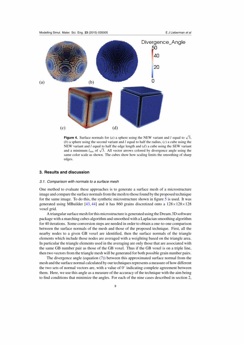
To highlight the effect of the size of the neighborhood, figure 4 shows the divergence anglebetween calculated normals and true normals for a sphere and a cube using different variants.The divergence angle is defined as the angle that exists between the surface normals generatedby this technique and the surface normals they are being compared against. The equation tocalculate the divergence angle is

θdiv = cos−1

( �vT · �vC

‖�vT ‖ ‖�vC‖)

. (7)

Here, �vT and �vC are the two surface normals being compared. For the first sphere (figure 4(a)),the NEW variant is used as the method of smoothing with l = √

3. These results highlight theissue of discretization (i.e. stair-stepping); by representing a smooth sphere as a collection ofcubes, the approximate surface is inherently rough, especially where it does not align well withthe mesh, and errors are made in the surface normal calculations. For the value of l = √

3,the result is an average divergence angle of ∼21◦. The result can be improved on by utilizinga larger value of l to achieve greater smoothing. For the second sphere (figure 4(b)), l is setto half the radius of the sphere, which results in a dramatically smaller average divergenceangle of ∼1◦. However, the penalty for using such a large footprint is illustrated for the firstcube (figure 4(c)). Here, the NEW variant is used with l set to half the cube edge length, andthe average divergence angle is found to be ∼14◦, where there is an excessive rounding of thecube corners. For the second cube (figure 4(d)), the third variant is used with the edges of thecube treated as triple points, which results in greater accuracy close to the edges of the cube.Setting the value of lmin to

√3, the average divergence angle decreases to ∼1◦.

These test cases emphasize that one should keep the neighborhood as small as possiblein order to avoid these corner-rounding effects, albeit that smaller neighborhoods can increasethe level of error arising from stair-steps. The SEW variant was constructed as a compromisebetween these factors. However, the location of the edges/triple junction must be known touse the third variant of the technique because they are utilized to determine lmin and suchinformation may not always be available.

8

Modelling Simul. Mater. Sci. Eng. 23 (2015) 035005 E J Lieberman et al

(a) (b)

(c) (d)

Figure 4. Surface normals for (a) a sphere using the NEW variant and l equal to√

3,(b) a sphere using the second variant and l equal to half the radius, (c) a cube using theNEW variant and l equal to half the edge length and (d) a cube using the SEW variantand a minimum lmin of

√3. All vector arrows colored by divergence angle using the

same color scale as shown. The cubes show how scaling limits the smoothing of sharpedges.

3. Results and discussion

3.1. Comparison with normals to a surface mesh

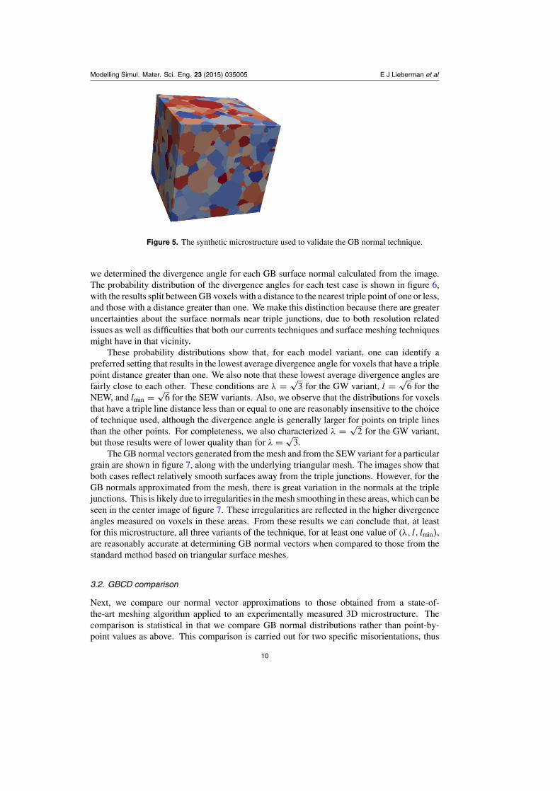
One method to evaluate these approaches is to generate a surface mesh of a microstructureimage and compare the surface normals from the mesh to those found by the proposed techniquefor the same image. To do this, the synthetic microstructure shown in figure 5 is used. It wasgenerated using MBuilder [43, 44] and it has 860 grains discretized onto a 128×128×128voxel grid.

A triangular surface mesh for this microstructure is generated using the Dream.3D softwarepackage with a marching cubes algorithm and smoothed with a Laplacian smoothing algorithmfor 40 iterations. Some conversion steps are needed in order to obtain a one-to-one comparisonbetween the surface normals of the mesh and those of the proposed technique. First, all thenearby nodes to a given GB voxel are identified, then the surface normals of the triangleelements which include those nodes are averaged with a weighting based on the triangle area.In particular the triangle elements used in the averaging are only those that are associated withthe same GB number pair as those of the GB voxel. Thus if the GB voxel is on a triple line,then two vectors from the triangle mesh will be generated for both possible grain number pairs.

The divergence angle (equation (7)) between this approximated surface normal from themesh and the surface normal calculated by our techniques represents a measure of how differentthe two sets of normal vectors are, with a value of 0◦ indicating complete agreement betweenthem. Here, we use this angle as a measure of the accuracy of the technique with the aim beingto find conditions that minimize the angles. For each of the nine cases described in section 2,

9

Modelling Simul. Mater. Sci. Eng. 23 (2015) 035005 E J Lieberman et al

Figure 5. The synthetic microstructure used to validate the GB normal technique.

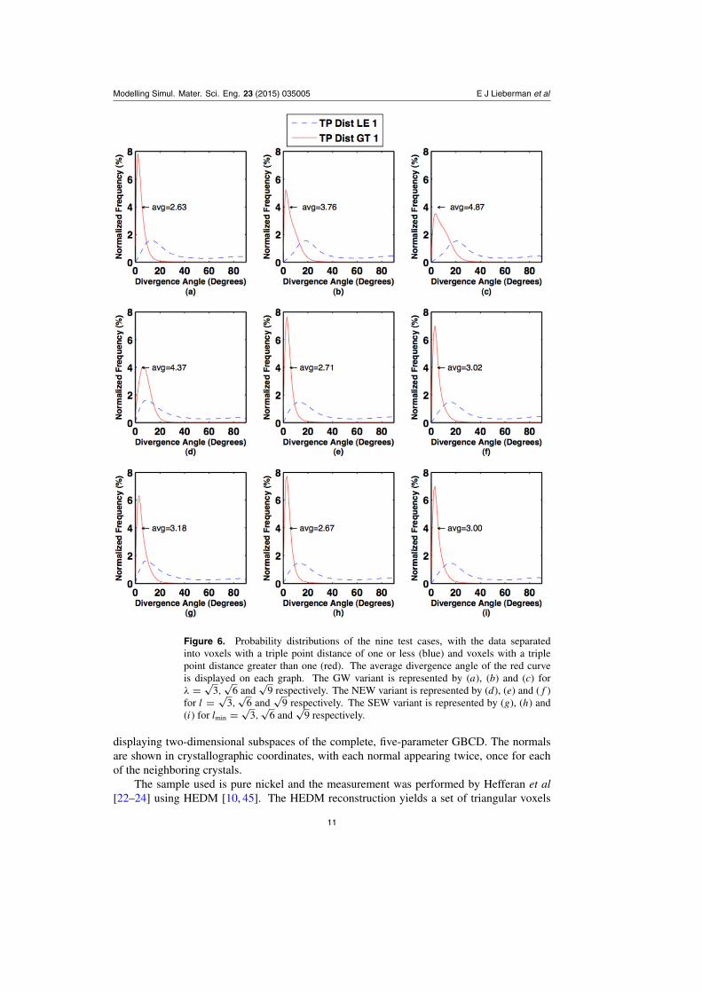
we determined the divergence angle for each GB surface normal calculated from the image.The probability distribution of the divergence angles for each test case is shown in figure 6,with the results split between GB voxels with a distance to the nearest triple point of one or less,and those with a distance greater than one. We make this distinction because there are greateruncertainties about the surface normals near triple junctions, due to both resolution relatedissues as well as difficulties that both our currents techniques and surface meshing techniquesmight have in that vicinity.

These probability distributions show that, for each model variant, one can identify apreferred setting that results in the lowest average divergence angle for voxels that have a triplepoint distance greater than one. We also note that these lowest average divergence angles arefairly close to each other. These conditions are λ = √

3 for the GW variant, l = √6 for the

NEW, and lmin = √6 for the SEW variants. Also, we observe that the distributions for voxels

that have a triple line distance less than or equal to one are reasonably insensitive to the choiceof technique used, although the divergence angle is generally larger for points on triple linesthan the other points. For completeness, we also characterized λ = √

2 for the GW variant,but those results were of lower quality than for λ = √

3.The GB normal vectors generated from the mesh and from the SEW variant for a particular

grain are shown in figure 7, along with the underlying triangular mesh. The images show thatboth cases reflect relatively smooth surfaces away from the triple junctions. However, for theGB normals approximated from the mesh, there is great variation in the normals at the triplejunctions. This is likely due to irregularities in the mesh smoothing in these areas, which can beseen in the center image of figure 7. These irregularities are reflected in the higher divergenceangles measured on voxels in these areas. From these results we can conclude that, at leastfor this microstructure, all three variants of the technique, for at least one value of (λ, l, lmin),are reasonably accurate at determining GB normal vectors when compared to those from thestandard method based on triangular surface meshes.

3.2. GBCD comparison

Next, we compare our normal vector approximations to those obtained from a state-of-the-art meshing algorithm applied to an experimentally measured 3D microstructure. Thecomparison is statistical in that we compare GB normal distributions rather than point-by-point values as above. This comparison is carried out for two specific misorientations, thus

10

Modelling Simul. Mater. Sci. Eng. 23 (2015) 035005 E J Lieberman et al

Figure 6. Probability distributions of the nine test cases, with the data separatedinto voxels with a triple point distance of one or less (blue) and voxels with a triplepoint distance greater than one (red). The average divergence angle of the red curveis displayed on each graph. The GW variant is represented by (a), (b) and (c) forλ = √

3,√

6 and√

9 respectively. The NEW variant is represented by (d), (e) and (f )for l = √

3,√

6 and√

9 respectively. The SEW variant is represented by (g), (h) and(i) for lmin = √

3,√

6 and√

9 respectively.

displaying two-dimensional subspaces of the complete, five-parameter GBCD. The normalsare shown in crystallographic coordinates, with each normal appearing twice, once for eachof the neighboring crystals.

The sample used is pure nickel and the measurement was performed by Hefferan et al[22–24] using HEDM [10, 45]. The HEDM reconstruction yields a set of triangular voxels

11

Modelling Simul. Mater. Sci. Eng. 23 (2015) 035005 E J Lieberman et al

Figure 7. GB normals for a particular grain are shown for the SEW model variantwith lmin = √

6 (left) and for the normals from the mesh (right), with the mesh itselfalso shown (center). The vectors are colored by the number of nearest-neighbor grains:blue = 1, orange = 2, red = 3.

(a) (b)

Figure 8. (a) Pure nickel microstructure from [22–24] has a resolution of1000×1000×71 points with spacing of 1.2×1.2×4 µm. (b) Surface mesh generatedfor this image. In both cases, the false color is based on randomly assigned grainnumber ID’s.

(in this case 1.2 µm side length equilateral triangles) in each of a set of 71 measured 2Dsections that are spaced in 4 µm intervals perpendicular to the section planes. This structurewas interpolated onto a cubic lattice, as shown in figure 8(a).

The GBs were meshed using a weighted Delaunay triangulation method developed byLi [46]. It utilizes algorithms available in the Computational Geometry Algorithms Library(CGAL) package.[47] with adaptations influenced by Boltcheva et al [48] to preserve importantfeatures, such as triple lines and quad points. The resulting mesh of this Ni microstructureis shown in figure 8(b) Using the meshed boundaries, Hefferan [23, 24] displayed the normaldistributions for two specific crystallographic misorientations, denoted as the �3 (60◦ rotationaround the 〈1 1 1〉 axis) and �9 (38.94◦ rotation around the 〈1 1 0〉 axis) boundaries. To generatethe GBCD, the GB surface normals are transformed into the crystallographic reference frameof their respective grains and then represented as a stereographic projection of the rotatedvectors, with only the GB points that have the misorientations of interest being included.Before rendering the vectors as a stereographic projection, the vectors are first transformedinto spherical coordinates and then binned by 10◦ intervals. The bins are then normalizedsuch that they are expressed as multiples of random density. The values of (λ, l, lmin) found insection 3 that resulted in the greatest accuracy for each variation of the technique are used togenerate GBCD from the HEDM images. The �3 GBCDs generated from the surface meshingand the three variants of the technique are shown in figure 9.

What we see from these GBCD is that each model variant shows a very similar distributionshape but the primary difference is in the spread and peak of the distributions. The GBCD that

12

Modelling Simul. Mater. Sci. Eng. 23 (2015) 035005 E J Lieberman et al

(a) (b)

(c) (d)

Figure 9. �3 GBCD (a) from [23, 24], (b) the GW variant of the proposed model withλ = √

3, (c) the second variant (NEW) with l = √6 and (d) the SEW variant with

lmin = √6. The strong peak in the upper right quadrant is associated with coherent twin

boundaries, which are very common in most annealed fcc metals such as the Ni studiedhere.

is closest to Hefferan’s �3 baseline, in terms of peak value, is obtained with the SEW variant,followed by the GW variant with the NEW variant being the least accurate. To quantify thiscomparison, figure 10 shows these same projections but colored by the value of the differencebetween with respect to Hefferan’s GBCD.

The largest absolute difference calculated in each case is 104.5 MRD for the GW variant,143.6 MRD for the NEW variant and 50.9 MRD for the SEW variant; these results are alsoshown in table 1. In particular, the largest difference for the SEW variant is not located at thestandard �3 GBCD peak, as it is for the other two.

The �9 GBCDs generated from the surface meshing and the three versions of the techniqueare shown in figure 11. Again the different variants of the technique show general agreementon the shape of the distribution but here there are more differences when compared to the �9baseline in that the peaks do not exactly line up, though they are all on the same 〈1 1 0〉 tiltprofile, and the secondary shapes in the distributions are also slightly different but occur in thesame positions in the plot. Again, the differences between the GBCD from Hefferan and theGBCD from this technique are shown in figure 12.

The largest absolute difference calculated in each case is 2.03 MRD for the GW variant,2.80 MRD for the NEW variant and 2.16 MRD for the SEW variant. These results are alsoshown in table 1. The NEW variant is the most different from Hefferan’s GBCD and is alsofarther from the other two variants, which are themselves quite similar in their differencescompared to Hefferan’s. Overall, the �9 GBCD from the technique have greater relativedifferences to Hefferan’s �9 GBCD, than for the �3 GBCD, though the magnitudes aresmaller.

13

Modelling Simul. Mater. Sci. Eng. 23 (2015) 035005 E J Lieberman et al

Figure 10. Difference in MRD values for �3 boundaries between Hefferan’s GBCDand the GBCD from (left) the GW variant, (center) the NEW variant and (right) theSEW variant.

Table 1. Peak Difference in MRD between the GBCD from Hefferan and the GBCDgenerated by the three variants for both �3 and �9 boundaries.

Difference in �3 GBCD (MRD) Difference in �9 GBCD (MRD)

GEW 104.5 2.03NEW 143.6 2.80SEW 50.9 2.16

In general, the GBCD obtained from the NEW variant exhibits the best agreement withHefferan’s. The explanation for why the NEW variant is favored here while in section 3.1all three had similar accuracy is that the resolution of the HEDM sample (71×106 voxels) isgreater than that of the synthetic microstructure (∼2×106 voxels) and this particular varianthas a consistent smoothing effect with increasing resolution while the other two are indifferentto resolution changes.

4. Conclusion

The proposed technique based on the use of first order Cartesian moments to calculate avoxelized field of grain boundary normals has been shown to compare favorably to normalsfound using surface meshing. When locally comparing the grain boundary normals obtained bythe proposed technique to those from a triangular mesh, the greatest differences are found nearthe triple junctions and quad points, regions which are known to have inconsistencies with thesmoothing due to most algorithms allowing triple junction nodes less freedom of positioningthan other grain boundary nodes. Elsewhere the differences between the mesh normals andthe normals generated by the technique are on average less than 3◦. Differences between thedifferent variants of the technique appear when tested on the higher resolution HEDM sample.The scaling, equal-weighting (SEW) variant is the one having the most success at replicating theGBCDs produced by Hefferan [23], which is reasonable considering that this variant is the onlyone to scale with resolution changes. This allows the smoothing to increase with increasingresolution and match the results of surface mesh smoothing that is indifferent to resolution.Thus the scaling, equal-weighting (SEW) variant is the best choice if one assumes that the

14

Modelling Simul. Mater. Sci. Eng. 23 (2015) 035005 E J Lieberman et al

(a) (b)

(c) (d)

Figure 11. �9 GBCD (a) from [23, 24], (b) the first variant (GW) of the proposedmodel with λ = √

3, (c) the NEW variant with l = √6 and (d) the SEW variant with

lmin = √6.

Figure 12. Difference in MRD values for �9 boundaries between Hefferan’s GBCDand the GBCD from (left) the first variant (GW), (center) the second variant (NEW) and(right) the third variant (SEW).

boundaries being considered are smooth. However, if the above does not hold or the triplejunction or other surface edge information is not known, then the Gaussian weighting (GW)variant, which had the next best success at replicating the GBCD, would be a viable optionas well. Potential uses of the technique include estimating triple junction dihedral angles andincorporation in crystal plasticity models of grain boundary effects on mechanical responses,

15

Modelling Simul. Mater. Sci. Eng. 23 (2015) 035005 E J Lieberman et al

such as slip transmission across the boundary [49] or by calculating surface tractions. Wenote that all of the methods exhibited higher divergence near the triple lines in the first surfacemesh comparison in part because of a combination of an effective high curvature at the cornersand the inability to recognize the transition between two different neighboring grains, whichshould give rise to a discontinuity in this simple definition of a surface normal. The additionof higher order moments/derivatives should improve the descriptions near the triple junctions.This aspect is currently being explored.

Acknowledgments

This work was supported by Los Alamos National Laboratory’s Directed Research andDevelopment (LDRD-DR Project 20140114DR) and the Institute for Materials Science. Wethank C M Hefferan, S F Li, J Lind and R M Suter for sharing the Ni data set and for helpfuldiscussions and assistance with interpretation. The data were collected at the Advanced PhotonSource, which is supported by the US Department of Energy, Office of Science, Office of BasicEnergy Sciences under contract number DE-AC02-06CH11357.

References

[1] Fensin S J et al 2014 Effect of loading direction on grain boundary failure under shock loadingActa Mater. 64 113–22

[2] Lin P, Palumbo G, Erb U and Aust K T 1995 Influence of grain boundary character distribution onsensitization and intergranular corrosion of alloy 600 Scr. Metall. Mater. 33 1387–92

[3] Randle V 2004 Twinning-related grain boundary engineering Acta Mater. 52 4067–81[4] Randle V, Rohrer G S, Miller H M, Coleman M and Owen G T 2008 Five-parameter grain

boundary distribution of commercially grain boundary engineered nickel and copper Acta Mater.56 2363–73

[5] Smith C S 1948 Introduction to grains, phases, and interfaces—an interpretation of microstructureTrans. AIME 175 15–51

[6] Saylor D M, Morawiec A and Rohrer G S 2003 The relative free energies of grain boundaries inmagnesia as a function of five macroscopic parameters Acta Mater. 51 3675–86

[7] Li J, Dillon S J and Rohrer G S 2009 Relative grain boundary area and energy distributions in nickelActa Mater. 57 4304–11

[8] Rohrer G S, Li J, Lee S, Rollett A D, Groeber M and Uchic M D 2010 Deriving grain boundarycharacter distributions and relative grain boundary energies from three-dimensional EBSD dataMater. Sci. Technol. 26 661–9

[9] Schwartz A J, Kumar M and Adams B L 2010 Electron Backscatter Diffraction in Materials Science2 edn (Dordrecht: Springer)

[10] Suter R M, Hennessy D, Xiao C and Lienert U 2006 Forward modeling method for microstructurereconstruction using x-ray diffraction microscopy: single-crystal verification Rev. Sci. Instrum.77 123905

[11] Saylor D M, El Dasher B S, Rollett A D and Rohrer G S 2004 Distribution of grain boundaries inaluminum as a function of five macroscopic parameters Acta Mater. 52 3649–55

[12] Saylor D M, El-Dasher B S, Adams B L and Rohrer G S 2004 Measuring the five-parameter grain-boundary distribution from observations of planar sections Metall. Mater. Trans. A 35 1981–9

[13] Dey T K and Goswami S 2004 Provable surface reconstruction from noisy samples Proc. 20thAnnual Symp. on Computational Geometry (Brooklyn, NY) vol 20 pp 330–9

[14] Hoppe H, DeRose T, Duchamp T, McDonald J and Stuetzle W 1992 Surface reconstruction fromunorganized points Comput. Graph. (ACM) 26 71–8

[15] Mitra N J, Nguyen A N and Guibas L 2004 Estimating surface normals in noisy point cloud dataInt. J. Comput. Geom. Appl. 14 261–76

16

Modelling Simul. Mater. Sci. Eng. 23 (2015) 035005 E J Lieberman et al

[16] Ivasishin O M, Shevchenko S V and Semiatin S L 2009 Implementation of exact grain-boundarygeometry into a 3-D Monte-Carlo (Potts) model for microstructure evolution Acta Mater.57 2834–44

[17] Moore D and Warren J 1991 Approximation of dense scattered data using algebraic surfaces Proc.24th Annual Hawaii Int. Conf. on System Sciences (Kauai, HI) vol i, pp 681–90

[18] Lorensen W E and Cline H E 1987 Marching cubes: a high resolution 3D surface constructionalgorithm SIGGRAPH Comput. Graph. 21 163–9

[19] Groeber M and Jackson M 2014 DREAM.3D: a digital representation environment for the analysisof microstructure in 3D Integr. Mater. Manuf. Innov. 3 5

[20] Saylor D M, Morawiec A and Rohrer G S 2003 Distribution of grain boundaries in magnesia as afunction of five macroscopic parameters Acta Mater. 51 3663–74

[21] Chandross M and Holm E A 2010 Measuring grain junction angles in discretized microstructuresMetall. Mater. Trans. A 41 3018–25

[22] Hefferan C M et al 2009 Statistics of high purity nickel microstructure from high energy x-raydiffraction microscopy Comput. Mater. Continua 14 207–17

[23] Hefferan C 2012 Measurement of annealing phenomena in high purity metals with near-field highenergy x-ray diffraction microscopy PhD Thesis Carnegie Mellon University

[24] Suter R M, Li S F, Hefferan C and Lind J, Thermally induced coarsening in a nickel polycrystalobserved in three dimensions, in preparation

[25] Kalogerakis E, Simari P, Nowrouzezahrai D and Singh K 2007 Robust statistical estimation ofcurvature on discretized surfaces Symp. on Geometry Processing (Barcelona, Spain) pp 13–22

[26] Garapic G, Faul U H and Brisson E 2013 High-resolution imaging of the melt distribution in partiallymolten upper mantle rocks: evidence for wetted two-grain boundaries Geochem. Geophys.Geosyst. 14 556–66

[27] Feng X, Xia K, Tong Y and Wei G-W 2012 Geometric modeling of subcellular structures, organelles,and multiprotein complexes Int. J. Numer. Methods Biomed. Eng. 28 1198–223

[28] Lebensohn R A, Brenner R, Castelnau O and Rollett A D 2008 Orientation image-basedmicromechanical modelling of subgrain texture evolution in polycrystalline copper Acta Mater.56 3914–26

[29] Lebensohn R A, Kanjarla A K and Eisenlohr P 2012 An elasto-viscoplastic formulation based onfast Fourier transforms for the prediction of micromechanical fields in polycrystalline materialsInt. J. Plast. 32–33 59–69

[30] Lebensohn R A, Escobedo J P, Cerreta E K, Dennis-Koller D, Bronkhorst C A and Bingert J F 2013Modeling void growth in polycrystalline materials Acta Mater. 61 6918–32

[31] MacSleyne J P, Simmons J P and De Graef M 2008 On the use of moment invariants for theautomated analysis of 3D particle shapes Modelling Simul. Mater. Sci. Eng. 16 045008

[32] Lo C-H and Don H-S 1989 3-D moment forms: their construction and application to objectidentification and positioning IEEE Trans. Pattern Anal. Mach. Intell. 11 1053–64

[33] Monga O and Benayoun S 1995 Using partial derivatives of 3D images to extract typical surfacefeatures Comput. Vis. Image Understand. 61 171–89

[34] Lindeberg T 1993 Discrete derivative approximations with scale-space properties: a basis for low-level feature extraction J. Math. Imag. Vis. 3 349–76

[35] Lindeberg T 1998 Edge detection and ridge detection with automatic scale selection Int. J. Comput.Vis. 30 117–56

[36] Tasdizen T, Whitaker R, Burchard P and Osher S 2003 Geometric surface processing via normalmaps ACM Trans. Graph. 22 1012–33

[37] Wang Y, Sheng Y, Lu G, Tian P and Zhang K 2008 Feature-constrained surface reconstructionapproach for point cloud data acquired with 3D laser scanner Proc. SPIE 7000 700021

[38] Apostol T M 1969 Calculus vol 2, 2nd edn (Waltham, MA: Xerox Publishing) sections 8.16 and12.1-3

[39] Guest P G 1961 Numerical Methods of Curve Fitting (New York: Cambridge University Press)especially chapters 6 and 7

Ryan T P 1997 Modern Regression Methods (New York: Wiley) especially chapters 1 and 8

17

Modelling Simul. Mater. Sci. Eng. 23 (2015) 035005 E J Lieberman et al

[40] Leclaire S, El-Hachem M, Trepanier J-Y and Reggio M 2014 High order spatial generalization of2D and 3D isotropic discrete gradient operators with fast evaluation on GPUs J. Sci. Comput.59 545–73

[41] Shima E, Kitamura K and Haga T 2013 Green–gauss/weighted-least-squares hybrid gradientreconstruction for arbitrary polyhedra unstructured grids AIAA J. 51 2740–7

[42] Lindeberg T 2011 Generalized Gaussian scale-space axiomatics comprising linear scale-space,affine scale-space and spatio-temporal scale-space J. Math. Imag. Vis. 40 36–81

[43] Saylor D, Fridy J, El-Dasher B, Jung K-Y and Rollett A 2004 Statistically representative three-dimensional microstructures based on orthogonal observation sections Metall. Mater. Trans. A35 1969–79

[44] Brahme A, Alvi M H, Saylor D, Fridy J and Rollett A D 2006 3D reconstruction of microstructurein a commercial purity aluminum Scr. Mater. 55 75–80

[45] Lienert U et al 2011 High-energy diffraction microscopy at the advanced photon source JOM63 70–7

[46] Li S F 2011 Imaging of orientation and geometry in microstructures: development and applicationsof high energy x-ray diffraction microscopy PhD Thesis Carnegie Mellon University

[47] Alliez P, Rineau L, Tayeb S, Tournois J and Yvinec M 2011 3D mesh generation CGAL User andReference Manual ed CGAL Editorial Board

[48] Boltcheva D, Yvinec M and Boissonnat J D 2009 Mesh generation from 3D multi-material images12th Int. Conf. on Medical Image Computing and Computer-Assisted Intervention (MICCAI2009) (Berlin, Germany, 20–24 September) pp 283–90

[49] Bieler T R et al 2009 The role of heterogeneous deformation on damage nucleation at grainboundaries in single phase metals Int. J. Plast. 25 1655–83

18