78 Philips tech. Rev. 39, 78-86, 1980, No. 3/4

Calculation and design of electro-mechanical devices

B. Aldefeld

In designing electro-mechanical devices it is desirable to have a quantitative knowledge of thephysical processes that determine their behaviour. These include the distribution of themagnetic field, the effects of eddy currents and the changes in the magnetic circuit caused by themotion of the armature. Computer calculations can be used to calculate the effects of a largenumber of parameters before a device is actually constructed. A t the Philips Hamburg labora-tories a computer program has been developed that can be used toprovide a rapid analysis of alarge number of variations to a design. The program provides accurate predictions of thedynamic behaviour of these devices.

Introduetion

Electro-mechanical devices (sometimes calledelectromagnetic devices) are driven by a magneticfield generated by an electric current flowing in a coilcombined with a suitably shaped iron circuit. Themagnetic field €?xertsforces on an armature of mag-netizable material, so that mechanical energy is pro-duced. Examples of such devices are electro-rnechan-ically actuated valves, brakes, clutches and printers.The calculation and design of such devices is the sub-ject of this article.

When electro-mechanical devices have to be newlydesigned or improved, preliminary calculations arenecessary to show whether the expected performancewill meet the target specifications. Accurate calcula-tions can reduce considerably the number of exper-imental investigations to be made. Such experimentsare not only expensive, but are extremely time-con-suming. They cannot be omitted altogether, ofcourse, for there are always some problems that defycalculation. Questions concerning matters such asdurability, resistance to wear and material processingare not amenable to mathematical treatment, andexperimental tests on prototypes are thereforeindispensable.As an example of an electro-mechanical device,

fig. 1 shows an electromagnet used in a dot-mosaicprinter. A printer of this type consists of a number ofneedles that can be separately actuated so as to pro-duce a character on paper. The electromagnets arerequired to meet the following specifications: an

Dr B. Aldefeld is with Philips GmbH ForschungslaboratoriumHamburg, Hamburg, West Germany.

available mechanical energy of about 1 m.I, a highspeed of action (repetition rate between 1000 and1500 Hz), accurate timing, high electro-mechanicalefficiency, and a long life. And of course the manu-facturing costs should be as low as possible.The conventional methods of computing the per-

formance of such devices are based on simplifiedanalytical expressions. These have their uses for ob-taining a general insight into idealized cases and forestimating the variation of certain quantities. How-ever, even for the simple geometry of the magnet infig. 1, these classical methods do not provide suf-ficiently accurate solutions. This is due in the firstplace to the nonlinearity of the magnetization curveof iron. This means that the permeability is dependenton the induction (magnetic flux density) B, so that thecontribution of the iron to the total magnetic fieldvaries in a manner that is not easily predictable.Another problem is that there are eddy currents if theiron is not laminated. Their intensity varies with spaceand time, and depends on several other factors suchas the shape of the iron circuit, the electrical con-ductivity and the magnetic permeability.

These problems can be tackled by means of suitablenumerical methods, known as finite-element andfinite-difference methods, which are also widely ap-plied in other fields, for instance in the calculation ofmechanical stresses [1]. These methods are baseddirectlyon the fundamental differential equations de-scribing the problem, making it possible to obtainresults with an accuracy that depends only on thecomputer time available.

Philips tech. Rev. 39, No. 3/4 ELECTRO-MECHANICAL DEVICES 79

For problems of a dynamic nature, however, whichwe are concerned with here, even the capabilities ofmodern computers are inadequate when it comes todealing with arbitrary three-dimensional problems.The computer time required would be far too long,for reasons that will become obvious when the nu-merical method used is described. Nevertheless, manyof the problems encountered in practice - such asgeometries with rotational symmetry - can in fact besolved because they are mathematically two-dimen-sional.

The investigation and development of numericalmethods of calculation for magnets with rotationalsymmetry has been the subject of several years ofwork at Philips Forschungslaboratorium Hamburg.The objective was the development of .a computerprogram that could be used as a design aid. Thisprogram, called EDDY (EDdy currents, DYnamicbehaviour) was completed towards the end of 1978.The methods on which it is based, the problems it cansolve and some results will be described in this article.

PN

12mm

Fig. 1. Electromagnetic actuator used in a dot-mosaic printer.C actuating coil. SI soft-iron core. PS pole pieces. A armature withprint needle PN. RS return spring, which returns the armature to itsinitial position after the needle has touched the paper. The magnetis energized by a current or voltage pulse lasting about 0.5 ms. Theprinted characters consist of patterns of single dots.

Basic equations

The behaviour of an electromagnet that is excitedby a variable current is largely described by two dif-ferential equations, one relating to the magnetic field,the other to the motion of the armature. Other rela-tions also enter into the picture. If the magnet isexcited from a voltage generator, the current depend-ent self-inductance of the system has to be calculated.If the magnet is excited by a very high current, heatgeneration may be a limiting factor. This is often thecase in practice.

Magnetic field

To compute the magnetic field throughout theentire magnetic circuit we make use of the vectorpotential, A, which can be derived at every point fromthe current distribution [2]. There is some analogybetween this vector potential, generated by currents,and the electrostatic potential, which arises fromcharges.

The derivation of an electric field-strength from theelectrostatic potential is well known. The potential isdefined at a point x,y,z as

1 J Q(V)rp(x,y,z) = - dV,4n80 rv(x,y,z)

where 80 is the permittivity of free space, Q(V) is thecharge density in the volume element dVand rv is thedistance between d V and the point x,y, z. Similarly thevector potential A (x,y,z) is defined as

/10 J j(V)A(x,y,z) = - dV,4n rv(x,y,z)

where /10 is the permeability of free space and j( V) isthe current densi ty in the volume element d V. Fromthe electrostatic potential the electric field-strength Ecan be derived by differentiation with respect to thecoordinates of position, or by applying the gradientoperator:

orp orp orpE = - grad rp = - - nx - - ny - - nz•

oX oy öz

The magnetic flux density B can be derived in muchthe same way from A by means of the relationB = curiA. The analogy between rp and A ends here,because rp is a scalar quantity and A is a vector.

Provided the current distributions are not too com-plicated, A has the same direction everywhere as thecurrent. In the magnets considered in this article weare only concerned with currents in the tangentialdirection of the cylindrical coordinates and thereforeA will also be tangential, that is to say the only non-zero component of A is A",.

In practical situations it is not easy to calculate thevector potential from the definition given above.However, we know from Maxwell's equations [3] that

curiB//1 = j,

[I] J. H. R. M. Eist and D. K. Wielenga, The finite-element meth-od and the ASKA program, applied in stress calculations fortelevision picture tubes, Philips tech. Rev. 37, 56-71, 1977.

[2] See for example J. Volger, Vortices, Philips tech. Rev. 32,247-258,1971.

[3] R. L. Stall, The analysis of eddy currents, chapter 1; Claren-don Press, Oxford 1974.

80 B. ALDEFELD Philips tech. Rev. 39, No. 3/4

and hence

curl(~ CUrlA) =L

where Jl. is the magnetic permeability of the material atthe point where we wish to calculate A, and j is thecurrent density. If this is converted into cylindricalcoordinates a differential equation is obtained, fromwhich A can be calculated. As stated earlier, the onlynon-zero component of A is the tangential A 'P. Thedifferential equation to be solved finally becomes [3]

~ (_1 ~ rAQJ\ + ~ (_1 ~rAQJ\ =or ru ()r ï ()Z ru ()Z ï

= _h+ (J (()AQJ + Vz ()AQJ). (1)()t ()Z

The last two terms on the right-hand side of theequation have been added to describe the effect of theeddy currents and the movement of the armature(0" is the electrical conductivity of the magneticmaterial and Vz is the velocity of the armature). Notethat the differential equation (1) is nonlinear, since thepermeability Jl. depends on the flux density, which inturn is a function of the vector potential.The differential equation describes the magnetic

field completely, because once it has been solved forthe vector potential, all other quantities of the electro-magnetic field can be found from simple relations.For instance, the components of the magnetic fluxdensity B are given by

1 ()Br = - - - rA QJ,

r ()Z

and

1 ()Bz = - - rAQJ.

r or

These relations follow directly from Maxwell's equa-tions.

Motion of the armature

If we assume that the armature can only move inthe z-direction, its motion is given by the equation

()2Z 1-2 = - (Fm + F, + Ff),()t m

where m is the mass of the armature; Fm, F, and Frdenote the axial components of the magnetic force,the spring force and the frictional force, in that order.

The force exerted on the movable parts of the mag-netic circuit by the magnetic field can be evaluated

from the flux-density distribution. This force is givenin integral form by the surface integral [4]:

Fm = /{ }_ B (B • n) - _1_ B2n} dS, (3)Jl.o 2Jl.o

where n is the vector normal to the surface elementdS. (The surface of integration can be freely chosen,provided that it completely encloses the movable partand does not interseet other magnetizable parts.)

Method of solution

(2)

General procedure

The equations given above are solved by time-step-ping methods. Time-stepping means that solutions tothe equations are calculated at small time intervals,with each new solution based on the previous one.Since the differential equations (1) and (2) are inter-dependent, they have to be solved simultaneously.(The equations are connected ('coupled') via themagnetic force and the position and velocity of thearmature.)If only static fields and forces are to be computed,

equation (2) is not relevant, and the right-hand side ofequation (1) only contains the current density, whichis constant. In the time-dependent case the solutionprocedure starts at the time t = 0, when the vectorpotential is zero throughout the geometry andthe armature is stationary in its initial position.Then, using small time steps, the two differentialequations are solved alternately until the final stateis reached.To improve the accuracy of the solution, a predic-

tion-correction method can be used at each time step.In the prediction phase the position of the armature ispredicted by solving eq. (2) on the assumption that themagnetic force has remained the same as the com-puted value of the previous step. The vector potentialfor this new position is then calculated from eq. (1),and from this the new magnetic force is calculatedfrom eq. (3). In the correction phase the differentialequation for the position of the armature is solvedagain, now using the new value for the magneticforce. The solution of the ordinary differential equa-tion (2) can now easily be obtained by means of well-known, fast and reliable methods, such as the Runge-Kutta procedure [5]. Such standard methods are notavailable for solving the nonlinear partial differentialequation (1). Here the search for improved techniquesis still in progress, with particular emphasis on thereduction of the computer time required. Themethods used in the EDDY program are described inthe next section.

Philips tech. Rev. 39, No. 3/4 ELECTRO-MECHANICAL DEVICES 81

Finite-difference method

The essential feature of the numerical methods forthe solution of a partial differential equation is thatthe equation is discretized, which means that solu-tions are only calculated for discrete points in spaceand time. The discretized analogue of the differentialequation is a set of algebraic equations, which isamenable to solution by computer. Once the solutionfor the discrete points has been obtained, an inter-polation procedure can be used to obtain the solutionfor the region between the points. The density of thepoints determines the accuracy to which the differen-tial equation is approximated. A denser distributiongives an improved accuracy, but also requires morecomputer time because the calculation has to be madefor more points. These methods are known as fini te-difference methods.

Discretization

To obtain the analogues of the partial derivativeswith respect to space, the geometry is considered to besubdivided into a number of elements by means of arectangular mesh. The nodes of the mesh define thepoints at which the value of the vector potential willbe calculated. In the case of rotational symmetry, it issufficient to discretize only half of the cross-sectionalarea.

As an example, fig. 2 shows such a mesh for theelectromagnet of fig. 1, together with the outline ofthe iron parts and the coil.

_j~ ;X

;X

r x Lx r--

><x X< .r:1 III

><xX<x ><x

><x~x~

Fig. 2. Example of a finite-difference mesh. The spacings of themesh (the mesh lengths) are variable, so that smaller spacings canbe used in regions where a more accurate solution is required, as inthe air-gap region. All elements are assigned values for the per-meability, conductivity, velocity, current density and magnetic fluxdensity.

A mesh of this type consists of horizontal and ver-tical lines that have points of intersection over thewhole region. It can be set up very easily, since onlytwo sets of lines have to be specified, and a fast al-gorithm can be found for modifying it in accordancewith the time-varying position of the armature. Inaddition, the resulting equations have a simple struc-ture, which also simplifies the numerical solution. Adisadvantage of this simple mesh is that shapes withcurved surfaces - other than those with rotationalsymmetry - are difficult to approximate.

A detailed description of the mathematical proce-dure for obtaining the discretized form of thedifferential equation would be beyond the scope ofthis article, but a procedure for a simplified case canbe explained briefly. Let us consider the differentialequation

()2A ()2A

+ -=0()X2 ()y2 '

which is a highly simplified form of eq. (1) in Cartesiancoordinates, with the right-hand side set equal to zero.Let the mesh in this simple case have a constant meshlength h, as shown infig. 3. The approximation to thefirst derivatives of the vector potential can then easilybe obtained from the ratios of the differences. For the

(4)

spatial derivative at a point half-way between nodes1+ 1, m and I,m, for example, this gives:

AA 1- = - (At+1,m - At,m).~x h

From these first derivatives an approximation to thesecond derivatives at the point I,m can be obtained inthe same way, giving for the second derivative to thex-coordinate:

~2A 1-h2 (At+1,m + At-I,m - 2At,m),

~X2

and a corresponding relation for ~ 2A / ~y2. The fini te-difference analogue of the differential equation (4) isthen

1hi (At+l,m +At-I,m + At,m+l + At,m-l - 4At,m) = 0,

(5)or

At,m = t (At+l,m + At-I,m + At,m+l + At,m-l)'

An expression such as (5) is called a five-point fini te-

[4] B. Aldefeld, Forces in electromagnetic devices, Comm. Proc.COMPUMAG Grenoble 1978, paper 8.1.

[5] R. Zurmühl, Praktische Mathematik für Ingenieure und Phy-siker, 5th edition, chapter 27; Springer, Berlin 1965.

82 B. ALDEFELD Philips tech. Rev. 39, No. 3/4

difference equation, since five nodes of the mesh areused in the expressions.

In the case of the more complicated differentialequation (1), a different procedure for the space dis-cretization is more suitable because the vector poten-

m

1-1,m+1 I, m-t 1+1,m

1-1, m l .rn 1+1,m

1-1, m-1 I, m-1 1+1,m1 h-I

Fig. 3. Section of a finite-difference mesh with a constant meshlength h. The indices l.m are used to identify the nodes.

tial cannot be differentiated at the boundaries of thematerial [6]. In addition, the time domain also has tobe discretized by introducing discrete time instants atintervals I:l.t. The result is again a five-point finite-difference equation which, somewhat simplified, hasthe form:

At+M = aAt + it+M + bAt+M + cAt+M +l.rn I,m Lrn l+l,m I-I,m

t+~t t+M+ dAI,m+1 + eAI,m-1 .

Here t denotes the time for which a solution hasalready been found, and t + I:l.tdenotes the new timefor which the solution is not yet known. The term it,mis the discretized current; a, b, c, d and e are coef-ficients that depend on the local values of permeabil-ity, conductivity, velocity and mesh length. Sincethere is a five-point equation for each node of themesh, there are as many equations as nodes. Theequations are all interdependent and can be assembledinto a matrix equation.

In practical applications the number of equationscan be considerable. Consider, for instance, a prob-lem in which the region of interest is subdivided into30 elements per coordinate direction: for rotationalsymmetry there are then 900 equations with 900 un-knowns to be solved at each time step. In an arbitrarythree-dimensional geometry, this becomes 27 000

equations with 27 000 unknowns at each time step. Anestimate of the computer time that would then beneeded shows that this method of solution would betoo cumbersome for most practical applications.

+1

Solving the finite-difference equations

For solving large numbers of equations with manyunknowns fast methods are available, such as Gaus-sian elimination. These methods are widely used inengineering calculations for buildings. However,methods of this type cannot be applied here, becausethe coefficients of the finite-difference equation (6) arenot constant but depend on the local flux density.Instead, a solution is obtained by means of aniterative process in which both the vector potentialand the coefficients are calculated. The method usedin the EDDY program is one of the class known asrelaxation methods. In these the vector potential iscalculated from the five-point equation (6), and theentire mesh is scanned repeatedly until eq. (6) issatisfied to a certain accuracy for all nodes. Thealgorithm consists in the following steps:1. Calculate the coefficients of eq. (6) from the valuesof the flux density of the preceding time step.2. Apply eq. (6) successively to all nodes of the meshto obtain the values of the vector potential Al,m.

3. Calculate the flux density from the vector potentialfor all cells of the mesh. Calculate the local per-meability from the flux density and the magnetizationcur-ve and determine the coefficients.4. Go back to step 2 and continue.s. Stop the procedure as soon as the differencesbetween successive values of the vector potential arebelow a specified limit.. In the EDDY program a number of improvements

that help to accelerate the convergence of the iterativeprocess have been introduced. First, instead of apply-ing the five-point equation to each single node, all thefive-point equations for all nodes on one mesh line aretreated simultaneously in a single matrix equation.This equation is solved by using a fast eliminationalgorithm [7], thus giving new values for all thenodes on a line simultaneously. The iteration consistsin repeated application of this procedure to all thelines of the mesh. This kind of technique is called 'lineiteration' .

Secondly, a method called 'overrelaxation' is used.This method is based on the fact that in each iterationthe values obtained for the vector potential, Al,m,

approach the solution only slowly by a relatively smallamount Ml,m. The increment Ml,m can thereforebe multiplied by a factor ca greater than 1, so that thesolution is approached more rapidly. (It can be shownthat the factor w, the 'overrelaxation' factor, must

h

-1

(6)

Philips tech. Rev. 39, No. 3/4 ELECTRO-MECHANICAL DEVICES 83

always be less than 2, otherwise the process would notconverge.)Thirdly, use is made of Maxwell's first equation,

which states, in its integral form, that the line integraloL the magnetic field-strength BI J1. around a closedpath must be equal to the number of ampere-turnsenclosed by the integration path. Accelerated conver-gence is achieved by evaluating the line integral aftereach iteration and correcting all values' of the vectorpotential in such a way that the integral criterion issatisfied.It should be noted that in the method described it is

necessary to take some precautions to ensure the con-vergence of the iterative process. Trouble may arisefrom the extreme nonlinearity of the magnetizationcurves of ferromagnetic materials. This is becauserelatively small differences in the flux density betweensuccessive iterations can cause large differences in thepermeability and hence in the coefficients of eq. (6).This may give rise to oscillations or even to diver-gence. If this effect is observed, it can be corrected bykeeping the changes in the coefficients below a certainlimit, e.g. by introducing an 'underrelaxation factor'(cv < 1), by analogy with the overrelaxation factor.

The EDDY computer program

The EDDY program was developed from the nu-merical methods outlined above, and is applicable tosystems with rotational symmetry. The solution pro-vides flux-density and eddy-current distributions,lines of force, energy losses, magnetic forces, motionof the armature and static temperature distributions.The program is written in standard FORTRANand consists of 70 subroutines with a total of about10000 lines of FORTRAN text. The maximumnumber of nodes it can handle is 5000, and thecore-storage requirement is 250 kbytes, with overlaytechniques.The user normally has to specify the initial input

data, which is summarized in Table J. If static mag-netic fields and forces only are to be calculated, someof this data is irrelevant and need not be specified. Ifthe static temperature distribution of the system is tobe calculated, the thermal conductivities must bespecified instead of the magnetization curves. Thecomputer time required for finding a solution variesconsiderably with the problem to be solved, and de-pends on several factors such as the shape of themagnetization curves and the number of nodes andtime steps. For the problems solved so far, the timerequired on a Philips PI400 has varied from fiveminutes to two hours for the calculation of thedynamic behaviour.

Application

The EDDY program has mainly been applied in thedesign of electromagnets used in dot-mosaic printers.Some of the many calculations performed will bedescribed below to illustrate the capacities of theprogram.

Static fields and forces

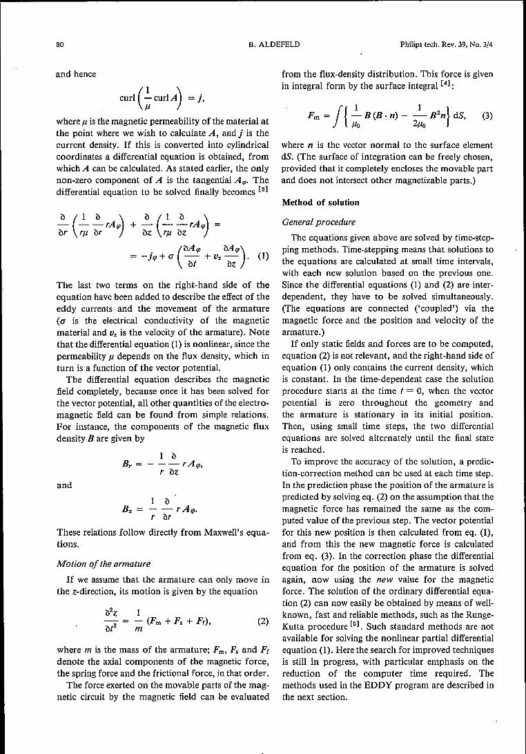
As a first step in design calculations for an electro-magnet, it is advisable to investigate static fields andforces alone. In this way a general picture of severalfeatures can be obtained with a minimum of com-puter time, and the information thus obtained can beused for estimating some of the dynamic quantities ifthe eddy-current effect is not too pronounced. Someexamples of such calculations are considered in figs 4,5 and 6. Figs 4a and 4b show the lines of force andthe flux-density distribution for the electromagnet offig. 1. Together these figures provide a complete pic-ture of the magnetic field, as they display both itsintensity and its direction. It should be noted that

\fig. 4b gives a relatively imprecise representation andthat more accurate flux-density values must be ob-tained from the tabular print-out.

Table I. Input data required for the EDDY computer program.

Configuration dimensions and shape of magnetic circuitand coil; number of turns and electricalresistance of coil; frictional force, initialspring tension and spring constant; elec-trical conductivity; magnetization curves

shape of current pulse at coil terminals

finite-difference mesh and time steps

relaxation factors; convergence criteria;max. permissible number ofiterations [*1

specifications relating to results of cal-culations (drawings, tables)

Excitation

Discretization

Parameters

Output

[*1 These parameters need only be specified if they differ from thevalues given in the program.

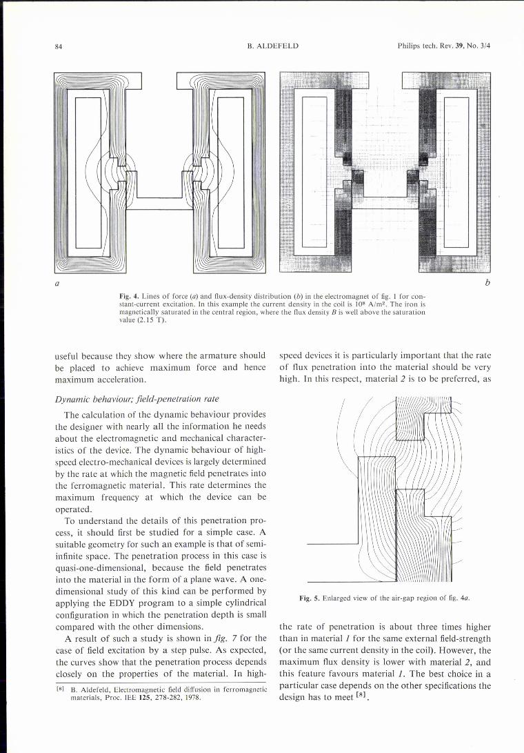
Fig. 5 gives an enlarged view of the air-gap regionof fig. 4a and shows the pattern of the lines of force inthis part of the magnet more clearly.The variation of the magnetic force as a function of

the displacement of the armature is shown infig. 6 fortwo values of the excitation current. These curves are

[61 R. L. StolI, The analysis of eddy currents, chapter 8; Claren-don Press, Oxford 1974.

[71 R. S. Varga, Matrix iterative analysis, chapter 6.4; Prentice-Hall, Englewood Cliffs 1962.

84 B.ALDEFELD Philips tech. Rev. 39, No. 3/4

a bFig. 4. Lines of force (a) and flux-density distribution (b) in the electromagnet of fig. I for con-stant-current excitation. In this example the current density in the coil is lOB A/m2• The iron ismagnetically saturated in the central region, where the flux density B is well above the saturationvalue (2.15 T).

useful because they show where the armature should speed devices it is particularly important that the ratebe placed to achieve maximum force and hence of flux penetration into the material should be verymaximum acceleration. high. In this respect, material 2 is to be preferred, as

Dynamic behaviour; field-penetration rate

The calculation of the dynamic behaviour providesthe designer with nearly all the information he needsabout the electromagnetic and mechanical character-istics of the device. The dynamic behaviour of high-speed electro-mechanical devices is largely determinedby the rate at which the magnetic field penetrates intothe ferromagnetic material. This rate determines themaximum frequency at which the device can beoperated.

To understand the details of this penetration pro-cess, it should first be studied for a simple case. Asuitable geometry for such an example is that of semi-infinite space. The penetration process in this case isquasi-one-dimensional, because the field penetratesinto the material in the form of a plane wave. A one-dimensional study of this kind can be performed byapplying the EDDY program to a simple cylindricalconfiguration in which the penetration depth is smallcompared with the other dimensions.

A result of such a study is shown in fig. 7 for thecase of field excitation by a step pulse. As expected,the curves show that the penetration process dependscloselyon the properties of the material. In high-

Is] B. Aldefeld, Electromagnetic field diffusion in ferromagneticmaterials, Proc. lEE 125, 278-282, 1978.

Fig. 5. Enlarged view of the air-gap region of fig. 40.

the rate of penetration is about three times higherthan in material 1 for the same external field-strength(or the same current density in the coil). However, themaximum flux density is lower with material 2, andthis feature favours material 1. The best choice in aparticular case depends on the other specifications thedesign has to meet [8].

Philips tech. Rev. 39, No. 3/4 ELECTRO-MECHANICAL DEVICES 85

10N

dzFig. 6. Static force Fm as a function of the armature displace-ment dz of the electromagnet in fig. 1. The excitation currents ofI A and 5 A correspond to current densities in the coil of 2 x 107and lOB A/m2• The force has its maximum value when the front ofthe armature is near the corner of the upper pole piece. The relati-vely small increase in the force as the current increases from I A to5 A is due to saturation of the magnetic circuit, particularly for thelarger displacements of the armature.

Fig. 7. Penetration of the magnetic field into a ferromagneticmaterial that fills a semi-infinite space, for the case where the fieldat the surface of the material is suddenly switched on and then re-mains constant. (In this example H = 4.8 X 104 A/m). The curves- flux density B as a function of depth x - which relate to dif-ferent materials, represent the flux waves at t = 0.1 ms after thefield has been switched on. Materiall has a saturation flux densityof 2.15 T and an electrical conductivity of 6 x 106 0-1 m-I. Formaterial2 the corresponding values are 1.7 Tand 7 x 105 0-1 m-I.The rate at which the field penetrates into the material is determinedby the eddy currents produced.

2.0TB

1.5

1.0

05

OL_----ll-----l-----~~--~~o 2 3 4mm

_X

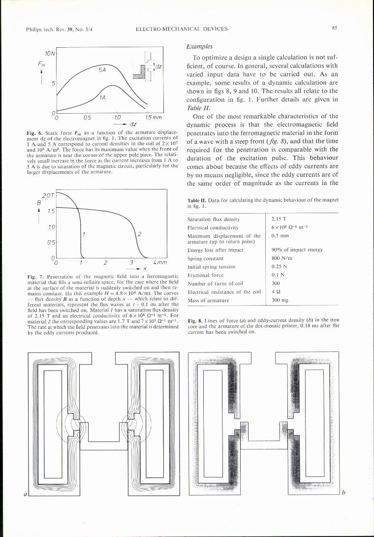
Examples

To optimize a design a single calculation is not suf-ficient, of course. In general, several calculations withvaried input data have to be carried out. As anexample, some results of a dynamic calculation areshown in figs 8, 9 and 10. The results all relate to theconfiguration in fig. 1. Further details are given inTable /l.

One of the most remarkable characteristics of thedynamic process is that the electromagnetic fieldpenetrates into the ferromagnetic material in the formof a wave with a steep front (jig. 8), and that the timerequired for the penetration is comparable with theduration of the excitation pulse. This behaviourcomes about because the effects of eddy currents areby no means negligible, since the eddy currents are ofthe same order of magnitude as the currents in the

Table 11. Data for calculating the dynamic behaviour of the magnetin fig. 1.

Saturation flux density

Electrical conductivity

Maximum displacement of thearmature (up to return point)

Energy loss after impact

Spring constan t

Initial spring tension

Frictional force

Number of turns of coil

Electrical resistance of the coil

Mass of armature

90070 of impact energy

800 N/m

0.25 N

0.1 N

300

40300 mg

2.15 T

6x 106 0-1 m-I

0.5 mm

Fig. 8. Lines of force (a) and eddy-current density (b) in the ironcore and the armature of the dot-mosaic printer, 0.18 ms after thecurrent has been switched on.

86 ELECTRO-MECHANICAL DEVICES Philips tech. Rev. 39, No. 3/4

coil. Another characteristic is that eddy currents stillcontinue to flow after the current in the coil hasdropped to zero. The eddy currents produce a fieldpattern in which most of the lines of force do not linkwith the coil but remain inside the iron (fig. 9). Theenergy for these currents is taken from the energy thatwas previously stored in the magnetic field.

Fig. 9. Lines of force 0.75 ms after switching on. The coil currenthas already dropped to zero, so that the eddy currents alone deter-mine the field pattern.

The importance of the eddy-current effect may beseen from a comparison of the curves in jig. JO. Thepower dissipated in the coil and the eddy-currentlosses are of nearly equal magnitude, but the mechan-ical energy is about four times lower. A reduction inthe eddy current will therefore be very effective inimproving the electra-mechanical efficiency.

Another undesired effect of eddy currents is thatthey cause the magnetic force to decay relativelyslowly after the excitation. This decelerates the arma-ture during its return phase, which in turn decreasesthe maximum possible repetition rate at which theprinter can operate. One remedy would be to use astronger return spring. This would at the same time

Summary. The behaviour of electro-mechanical devices can be cal-culated to a high accuracy by means of numerical computer meth-ods. The EDDY program developed at Philips Forschungslabora-torium Hamburg is based on a finite-difference method. The non-linear partial differential equation that describes the problem issolved by means of a relaxation technique with accelerated con-

0.25 0.5 o.7Sms

6 f-----t------~ - - - 2A/div-- 2V/div_.- 0.1mm/div6

t-. '-.

0.5 o.75ms-t

Fig. 10. Some of the curves describing the dynamic behaviour ofthe dot-mosaic printer during the first 0.75 ms after the current isswitched on. J Energy dissipated in coil. 2 Energy dissipated byeddy currents in the magnetic material. 3 Mechanical energy of thearmature. 4 Current in the coil. 5 Magnetic force. 6 Displacementof the armature.

have the positive effect of decreasing the mechanicalenergy, which is too high in the present example;about 1 ml is sufficient to actuate a print needle.

The example given makes it clear that a large num-ber of parameters can be varied. The EDDY programcan be used for calculating large numbers of dif-ferently combined parameters, enabling an optimumdesign to be found within a short time. This designcan then be constructed and tested.

The work described here was sponsored by theGerman Federal Ministry for Research and Technol-ogy under contract HH-PHII103. Responsibility forthe contents of this article rests with the author.

vergence. EDDY can be used for calculating the static and dynamicbehaviour of devices that have rotational symmetry. The solutionprovides the distribution of the magnetic field and the eddycurrents, the energy consumption, the losses, the magnetic forcesand the motion of the armature. EDDY has mainly been used in thedesign of dot-mosaic printers.