Calculating Areas and Lengths in ArcGIS10.2.2 … Areas and...Version_14Mar2015 Calculating Areas...
10
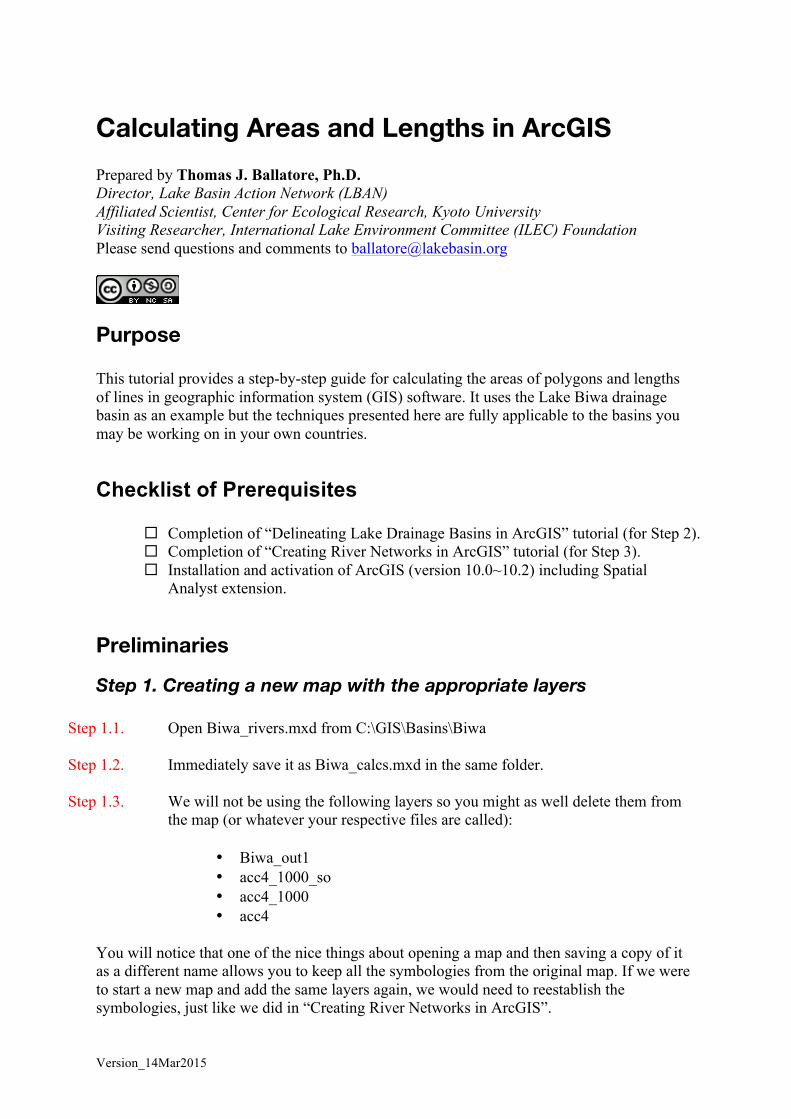
Version_14Mar2015 Calculating Areas and Lengths in ArcGIS Prepared by Thomas J. Ballatore, Ph.D. Director, Lake Basin Action Network (LBAN) Affiliated Scientist, Center for Ecological Research, Kyoto University Visiting Researcher, International Lake Environment Committee (ILEC) Foundation Please send questions and comments to [email protected] Purpose This tutorial provides a step-by-step guide for calculating the areas of polygons and lengths of lines in geographic information system (GIS) software. It uses the Lake Biwa drainage basin as an example but the techniques presented here are fully applicable to the basins you may be working on in your own countries. Checklist of Prerequisites Completion of “Delineating Lake Drainage Basins in ArcGIS” tutorial (for Step 2). Completion of “Creating River Networks in ArcGIS” tutorial (for Step 3). Installation and activation of ArcGIS (version 10.0~10.2) including Spatial Analyst extension. Preliminaries Step 1. Creating a new map with the appropriate layers Step 1.1. Open Biwa_rivers.mxd from C:\GIS\Basins\Biwa Step 1.2. Immediately save it as Biwa_calcs.mxd in the same folder. Step 1.3. We will not be using the following layers so you might as well delete them from the map (or whatever your respective files are called): • Biwa_out1 • acc4_1000_so • acc4_1000 • acc4 You will notice that one of the nice things about opening a map and then saving a copy of it as a different name allows you to keep all the symbologies from the original map. If we were to start a new map and add the same layers again, we would need to reestablish the symbologies, just like we did in “Creating River Networks in ArcGIS”.
Transcript of Calculating Areas and Lengths in ArcGIS10.2.2 … Areas and...Version_14Mar2015 Calculating Areas...
Version_14Mar2015
Calculating Areas and Lengths in ArcGIS Prepared by Thomas J. Ballatore, Ph.D. Director, Lake Basin Action Network (LBAN) Affiliated Scientist, Center for Ecological Research, Kyoto University Visiting Researcher, International Lake Environment Committee (ILEC) Foundation Please send questions and comments to [email protected]
Purpose This tutorial provides a step-by-step guide for calculating the areas of polygons and lengths of lines in geographic information system (GIS) software. It uses the Lake Biwa drainage basin as an example but the techniques presented here are fully applicable to the basins you may be working on in your own countries.
Checklist of Prerequisites
¨ Completion of “Delineating Lake Drainage Basins in ArcGIS” tutorial (for Step 2). ¨ Completion of “Creating River Networks in ArcGIS” tutorial (for Step 3). ¨ Installation and activation of ArcGIS (version 10.0~10.2) including Spatial
Analyst extension.
Preliminaries
Step 1. Creating a new map with the appropriate layers
Step 1.1. Open Biwa_rivers.mxd from C:\GIS\Basins\Biwa
Step 1.2. Immediately save it as Biwa_calcs.mxd in the same folder.
Step 1.3. We will not be using the following layers so you might as well delete them from the map (or whatever your respective files are called):
• Biwa_out1 • acc4_1000_so • acc4_1000 • acc4
You will notice that one of the nice things about opening a map and then saving a copy of it as a different name allows you to keep all the symbologies from the original map. If we were to start a new map and add the same layers again, we would need to reestablish the symbologies, just like we did in “Creating River Networks in ArcGIS”.

2
You should have something like the following right now:
Calculating Areas of Polygon Features In our previous work we have made two polygons for which we would like to know the area: Lake_Biwa.shp and basin4.shp (the Lake Biwa drainage basin). Calculating area is not as straightforward in ArcGIS as you might assume it would be for a “geographic” information system. Surprisingly, there is no “area” command or tool! There are three things we must do to calculate area: (1) either re-project the target shapefile (a polygon in this case) or change the Data Frame Properties to have a Projected Coordinate System (currently, we have a Geographic Coordinate System which means the data is measures in degrees and hence area calculations are not meaningful), (2) add a field to the target polygon’s Attribute Table in which we (3) make the actual area calculation. Let’s approach these in order.
Step 2. Setting a Projected Coordinate System So far, we have been working in the format the SRTM3 data comes in, i.e. Geographic Coordinate System with the WGS84 datum. ArcGIS labels this GCS_WGS_84. If you right click on any of the layers in the current map, open Layer Properties and go to the Source tab and scroll down a bit, you will see that the Spatial Reference is GCS_WGS_84. Also note that the units are “Decimal degrees”. For dem2, this looks like:

3
If we calculated area with this setting, we would get a result in square degrees which is meaningless. (Note: Until ArcGIS 9.2, it was possible to make this mistake. From 9.3 through the 10.2 we are using, the software will not even allow you to make this mistake by “disabling” the area command.) There are two main ways of dealing with this issue. For now, we will choose the fastest which is:
Step 2.1. Right click somewhere in the Data Frame (where the map appears) and choose Data Frame Properties.
Step 2.2. Select the Coordinate System tab and navigate to Projected Coordinate Systems | UTM | WGS 1984 and select WGS_1984_UTM_Zone_53N as shown below:

4
This is the UTM zone for Japan. It preserves areas, shapes and distances very well and is a popular projection for maps made in the Biwa area. You will note that when you apply this projection, the maps “shifts” and appears to be a bit narrower.
Step 3. Adding a Field to an Attribute Table Let’s start by calculating the area of the Lake_Biwa.shp file.
Step 3.1. Open its Attribute Table. You will see this:
Step 3.2. Click on the upper left “Table Options” icon.
5
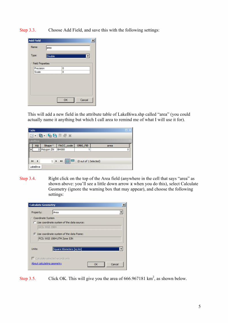
Step 3.3. Choose Add Field, and save this with the following settings:
This will add a new field in the attribute table of LakeBiwa.shp called “area” (you could actually name it anything but which I call area to remind me of what I will use it for).
Step 3.4. Right click on the top of the Area field (anywhere in the cell that says “area” as shown above: you’ll see a little down arrow when you do this), select Calculate Geometry (ignore the warning box that may appear), and choose the following settings:
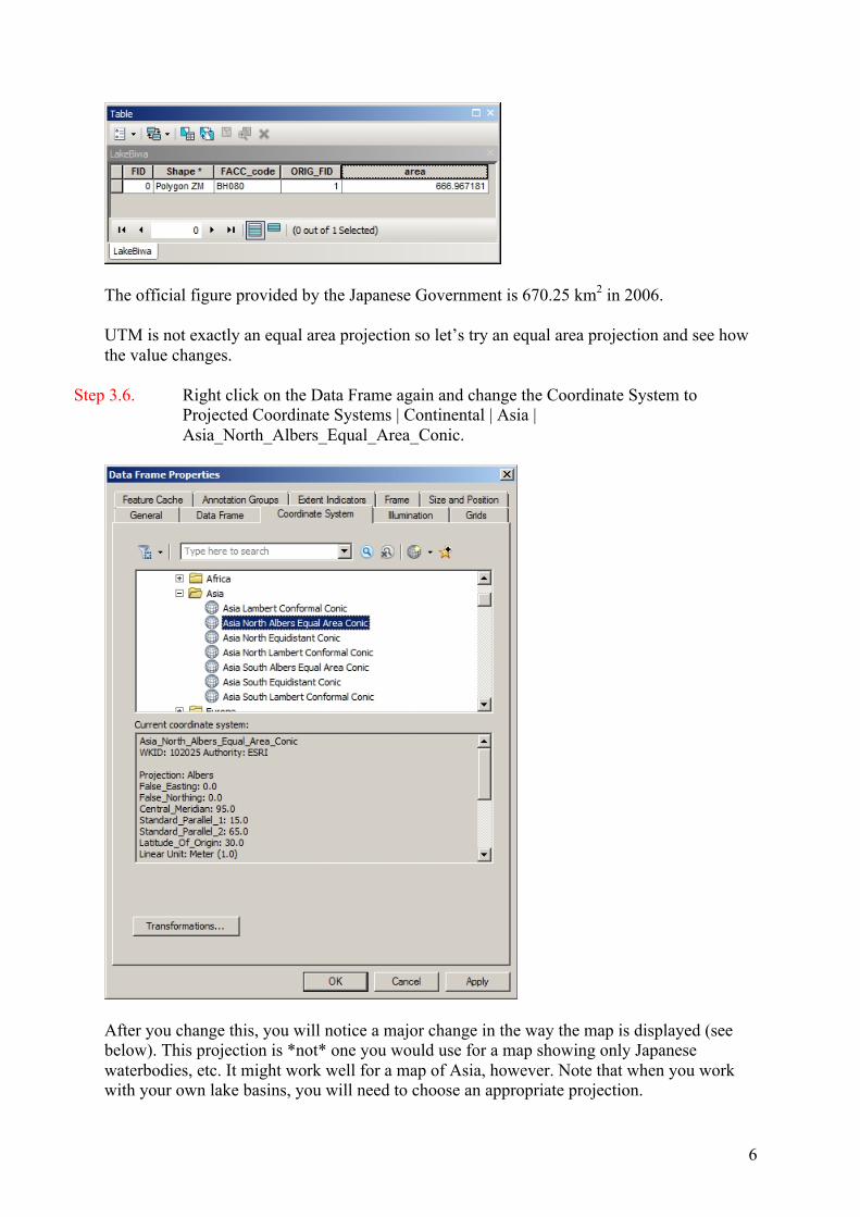
Step 3.5. Click OK. This will give you the area of 666.967181 km2, as shown below.
6
The official figure provided by the Japanese Government is 670.25 km2 in 2006. UTM is not exactly an equal area projection so let’s try an equal area projection and see how the value changes.
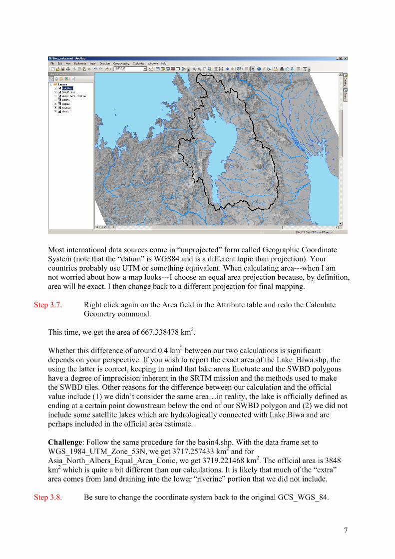
Step 3.6. Right click on the Data Frame again and change the Coordinate System to Projected Coordinate Systems | Continental | Asia | Asia_North_Albers_Equal_Area_Conic.
After you change this, you will notice a major change in the way the map is displayed (see below). This projection is *not* one you would use for a map showing only Japanese waterbodies, etc. It might work well for a map of Asia, however. Note that when you work with your own lake basins, you will need to choose an appropriate projection.
7
Most international data sources come in “unprojected” form called Geographic Coordinate System (note that the “datum” is WGS84 and is a different topic than projection). Your countries probably use UTM or something equivalent. When calculating area---when I am not worried about how a map looks---I choose an equal area projection because, by definition, area will be exact. I then change back to a different projection for final mapping.
Step 3.7. Right click again on the Area field in the Attribute table and redo the Calculate Geometry command.
This time, we get the area of 667.338478 km2. Whether this difference of around 0.4 km2 between our two calculations is significant depends on your perspective. If you wish to report the exact area of the Lake_Biwa.shp, the using the latter is correct, keeping in mind that lake areas fluctuate and the SWBD polygons have a degree of imprecision inherent in the SRTM mission and the methods used to make the SWBD tiles. Other reasons for the difference between our calculation and the official value include (1) we didn’t consider the same area…in reality, the lake is officially defined as ending at a certain point downstream below the end of our SWBD polygon and (2) we did not include some satellite lakes which are hydrologically connected with Lake Biwa and are perhaps included in the official area estimate. Challenge: Follow the same procedure for the basin4.shp. With the data frame set to WGS_1984_UTM_Zone_53N, we get 3717.257433 km2 and for Asia_North_Albers_Equal_Area_Conic, we get 3719.221468 km2. The official area is 3848 km2 which is quite a bit different than our calculations. It is likely that much of the “extra” area comes from land draining into the lower “riverine” portion that we did not include.
Step 3.8. Be sure to change the coordinate system back to the original GCS_WGS_84.
8
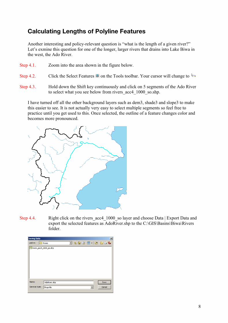
Calculating Lengths of Polyline Features Another interesting and policy-relevant question is “what is the length of a given river?” Let’s exmine this question for one of the longer, larger rivers that drains into Lake Biwa in the west, the Ado River.
Step 4.1. Zoom into the area shown in the figure below.
Step 4.2. Click the Select Features on the Tools toolbar. Your cursor will change to
Step 4.3. Hold down the Shift key continuously and click on 5 segments of the Ado River to select what you see below from rivers_acc4_1000_so.shp.
I have turned off all the other background layers such as dem3, shade3 and slope3 to make this easier to see. It is not actually very easy to select multiple segments so feel free to practice until you get used to this. Once selected, the outline of a feature changes color and becomes more pronounced.
Step 4.4. Right click on the rivers_acc4_1000_so layer and choose Data | Export Data and export the selected features as AdoRiver.shp to the C:\GIS\Basins\Biwa\Rivers folder.
9
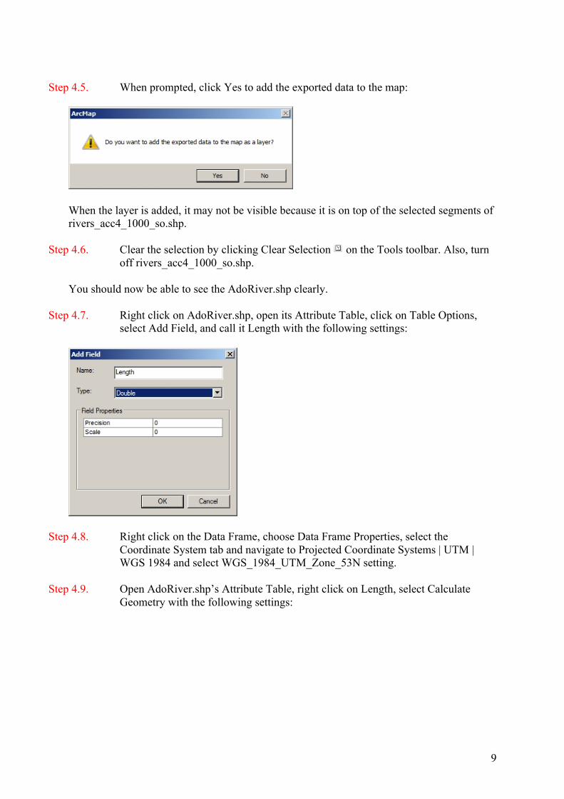
Step 4.5. When prompted, click Yes to add the exported data to the map:
When the layer is added, it may not be visible because it is on top of the selected segments of rivers_acc4_1000_so.shp.
Step 4.6. Clear the selection by clicking Clear Selection on the Tools toolbar. Also, turn off rivers_acc4_1000_so.shp.
You should now be able to see the AdoRiver.shp clearly.
Step 4.7. Right click on AdoRiver.shp, open its Attribute Table, click on Table Options, select Add Field, and call it Length with the following settings:
Step 4.8. Right click on the Data Frame, choose Data Frame Properties, select the Coordinate System tab and navigate to Projected Coordinate Systems | UTM | WGS 1984 and select WGS_1984_UTM_Zone_53N setting.
Step 4.9. Open AdoRiver.shp’s Attribute Table, right click on Length, select Calculate Geometry with the following settings:
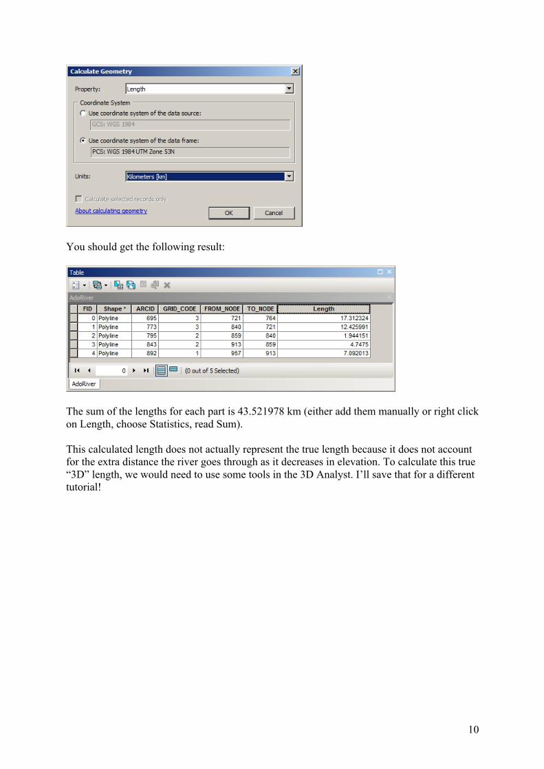
10
You should get the following result:
The sum of the lengths for each part is 43.521978 km (either add them manually or right click on Length, choose Statistics, read Sum). This calculated length does not actually represent the true length because it does not account for the extra distance the river goes through as it decreases in elevation. To calculate this true “3D” length, we would need to use some tools in the 3D Analyst. I’ll save that for a different tutorial!