Calcite Mineral Scaling Potentials of
97
Transcript of Calcite Mineral Scaling Potentials of
i
Calcite Mineral Scaling Potentials of High-Temperature Geothermal Wells
Alvin I. Remoroza
Faculty of Science University of Iceland
2010


iii
Calcite Mineral Scaling Potentials of High-Temperature Geothermal Wells
Alvin I. Remoroza
60 ECTS thesis submitted in partial fulfillment of a Magister Scientiarum degree in Geology (Geochemistry)
Advisor Prof. Stefán Arnórsson
External Examiner Ingvi Gunnarsson
Faculty of Science School of Engineering and Natural Sciences
University of Iceland Reykjavik, June 2010
iv
Calcite Mineral Scaling Potentials of High-Temperature Geothermal Wells 60 ECTS thesis submitted in partial fulfillment of a Magister Scientiarum degree in Geology (Geochemistry) Copyright © 2010 Alvin I. Remoroza All rights reserved Faculty of Science School of Engineering and Natural Sciences University of Iceland Sturlugötu 7 101 Reykjavik Iceland Telephone: 525 4000 Bibliographic information: Remoroza, A.I., 2010, Calcite Mineral Scaling Potentials of High-Temperature Geothermal Wells, Master’s thesis, Faculty of Science, University of Iceland, pp. 99. Printing: Háskólaprent ehf. Reykjavik, Iceland, June 2010
v
Abstract A comparative assessment of the calcite precipitation potential of geothermal fluids from some of the Hengill-Hellisheidi geothermal wells in Iceland, Pataan wells in Northern Negros, Philippines, and Mahanagdong wells in Leyte, Philippines are presented in this paper. The wells from these geothermal fields represent the varying characteristics of geothermal fluid discharges in different settings, ranging in composition from dilute to high salinities, and from different host rocks, i.e. basaltic and andesitic.
Water and gas analyses from the wells were used to calculate aquifer fluid compositions using the speciation program WATCH version 2.1. The total fluid enthalpy approaching that of saturated steam when the total discharge SiO2 approaches zero and Na/K and quartz temperature analysis are taken to indicate that “excess” enthalpy is mostly caused by phase segregation in the producing aquifers of Hellisheidi, Mahanagdong and Pataan wells. Plots of Na/K versus H2S temperatures and quartz versus H2S temperatures of closed system and phase segregation models substantiate the conclusion that “excess” enthalpy is mostly caused by phase segregation in producing aquifer. Phase segregation model was therefore used to calculate aquifer fluid compositions.
The selected phase segregation temperature correspond to saturation vapour pressure haftway between the sampling vapour pressure and the saturation vapour pressure of the selected aquifer temperature. Selected aquifer temperature was based on quartz temperature.
The mean differences between quartz and cation geothermometers for individual wells are within 5% (13 oC) except for very high enthalpy wells HE29 and MG40, and for most of the Pataan wells. No wells exceeded 10% mean percentage differences. The mean percentage difference for all the wells is 4 % (11 oC).
Evaluation of mineral-gas equilibria indicate that H2S aquifer fluid concentrations of Hellisheidi and Pataan wells are controlled by pyrite-pyrrhotite-magnetite or pyrite-pyrrhotite-prehnite-epidote mineral assemblage. Mahanagdong wells are systematically above the equilibrium magnetite-hematite-pyrite mineral assemblage by about 2000J/mol which is within the limit of error according to the data on enthalpy reported by Holland and Powell (1998) on these minerals. Hellisheidi’s H2 concentrations are found to be controlled by pyrite-pyrrhotite-magnetite or pyrite-pyrrhotite-prehnite-epidote mineral assemblage while Mahanagdong and Pataan are controlled by magnetite-hematite mineral assemblage. CO2 concentrations of Hellisheidi are consistently lower than equilibrium while Mahanagdong and Pataan wells are slightly above or at equilibrium with clinozoisite-calcite-quartz-prehnite or clinozoisite-calcite-quartz-grossular mineral assemblage. One cause of the low CO2 values at Hellisheidi may be insufficient supply of this gas to the fluid.
Aquifer fluid composition calculations show Hellisheidi’s pH range is alkaline to slightly alkaline (7-7.4). Mahanagdong’s pH is near neutral around 5.5 (5.3 – 5.9). Pataan wells have slightly acidic pH (4.9 – 5.6). Hellisheidi wells have higher concentrations of aqueous H2 (up to 8 ppm) compared to Mahanagdong and Pataan wells (less than 0.5 ppm). Hellisheidi wells also have higher concentrations of H2S of up to 250 ppm compared to Mahanagdong (<140 ppm) and Pataan (<200 ppm) wells. Pataan wells have the highest
vi
CO2 concentration of up to 9700 ppm, followed by Mahanagdong with up to 5300 ppm. Hellisheidi wells are the lowest, with less than 900 ppm.
Generally, the aquifer fluids are very close to equilibrium with calcite, and when all uncertainties were considered such as analytical imprecision and selection of aquifer temperatures, departure from saturation is not significant. The average departure from calcite saturation of Hellisheidi aquifer fluids is only 0.05 SI units, Mahanagdong and Pataan are both 0.2 SI units. Well PT02 from Pataan is the most oversaturated with 0.74 SI units.
The calculated saturation index for calcite increases with increasing value of the calculated aquifer pH. This is considered to be due to error in the calculated aquifer water pH. Many factors affect the calculated pH and it is not possible to identify the main sources of apparent variation in pH and calcite saturation index but it seems to be significant, particularly in the case of Hellisheidi.
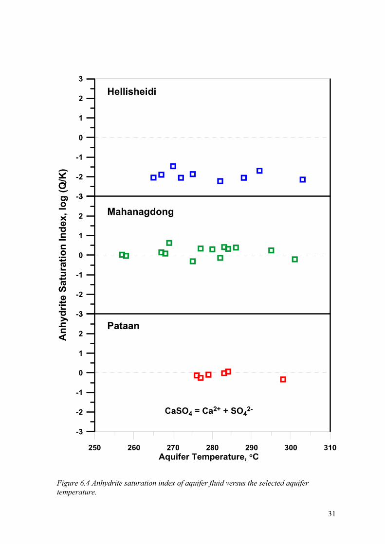
Mahanagdong and Pataan aquifer fluids approach anhydrite equilibrium whereas Hellisheidi waters are considerably anhydrite undersaturated.
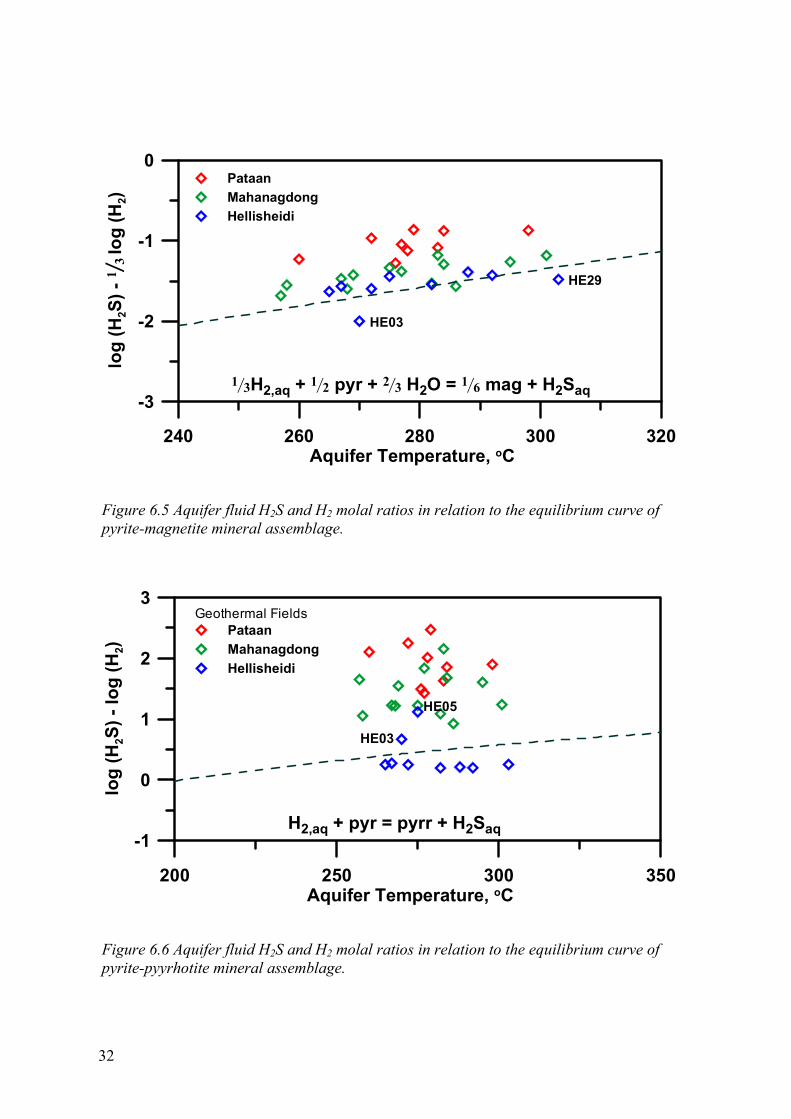
The Hellisheidi waters are close to the mineral-gas equilibrium curve for the redox reactions involving pyrite, magnetite, H2S and H2, with an average of 0.03 log units above the curve. Mahanagdong and Pataan aquifer waters are systematically with higher H2S/H2 ratios than those corresponding to equilibrium, by 0.2 and 0.55 log units on average, respectively.
Hellisheidi waters are also close to mineral-gas equilibrium curve for the redox reactions involving pyrite, pyrrhotite, H2S and H2 yet systematically below the equilibrium curve on average by 0.25 log units. Mahanagdong and Pataan aquifer waters are systematically with higher H2S/H2 ratios than those corresponding to equilibrium, by 0.96 and 1.3 log units on average, respectively. Clearly the H2S/H2 ratios in the aquifer waters in the Philippine geothermal fields are not controlled by pyrite-pyrrhotite buffer.
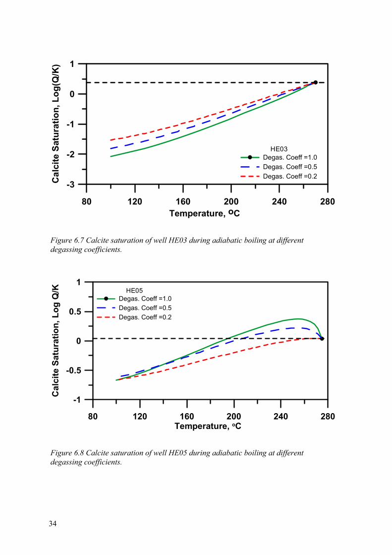
An overall pattern in the variation of the saturation index (SI) with temperature upon boiling and degassing of Hellishedi wells is observed. The SI initially increases then, after it reaches a peak, decreases to negative values. The initial increase in SI reflects an increase in pH due to CO2 and H2S degassing. The extent of degassing increases the level of calcite SI except for degassed well HE03 which shows the opposite. This well receives degassed fluid.
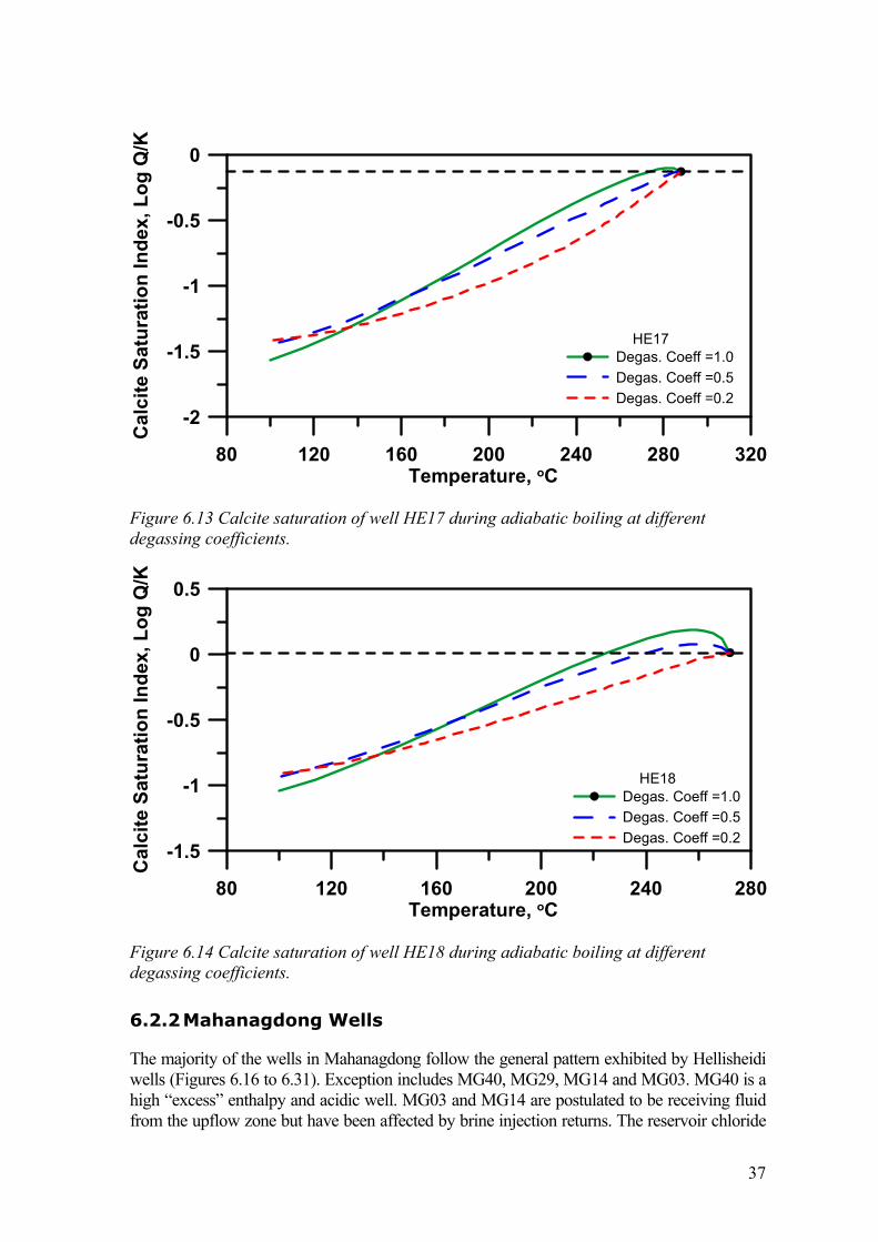
The majority of the wells in Mahanagdong followed the general pattern exhibited by Hellisheidi wells except MG40, MG29, MG14, and MG03. MG40 is a high “excess” enthalpy and acidic well. MG03 and MG14 were postulated to receive fluid from the upflow zone but have been affected by brine injection returns. The reservoir chloride levels of MG03 and MG14 are shifted towards the composition of the injected brine. Well MG29, on the other hand, is located on the western periphery of the Mahanagdong geothermal system and could be affected by intrusion of cooler peripheral waters. The highest positive departure from the initial saturation in Mahanagdong is from MG19, with 0.40 (at 251 oC) SI units above the initial saturation at degassing coefficient of 1.0. MG19 is thought to deposit calcite scale in the well.
vii
Comparing MG01 CO2 and H2S concentrations on samples taken in 2009 and 1994 show that they have been partially degassed or mixed with degassed injected brine. Aquifer aqueous CO2 concentration decreased from 8000 to 1200 ppm and H2S concentration decreased from 92 to 15 ppm. Activity of free Ca2+ affects calcite saturation because it increased (from 10 to 16 ppm) in 1994 to 2009 samples. Boiling of MG01 aquifer fluid sampled in 1994 produces an increase in calcite saturation of 0.51 SI units above the initial saturation which is high compared to the more recent sample with only 0.07 SI units departure from the initial saturation.
The case of well MG19 is similar with MG01, with the present fluid discharge partially degassed or mixed with injected brine and Ca2+ concentration has increased. Calcite mineral SI trend of MG19 practically remains the same after almost 15 years of production.
Pataan aquifer fluids show similar trends to those of Hellisheidi and most of the Mahanagdong wells with PT08 having the highest departure of 0.6 SI units (at 223 oC) above the initial saturation, followed by PT05, PT10 and PT07 with 0.40 (at 246 oC), 0.31(at 258 oC) and 0.28 (at 252 oC) SI units above the the initial saturation, respectively. PT05 was postulated to be nearest to the upflow region followed by PT08 and PT07. Well PT05 has the highest dissolved aqueous CO2 concentration at 9700 ppm, followed by PT08 and PT07 at 7800 and 6700 ppm, respectively. Wells PT02 and PT04 have the lowest positive departure from the initial saturation at 0.10 (at 262 oC) and 0.15 (at 262 oC) SI units above the initial saturation, respectively.
The effect of fluid mixing particularly the injected separated water from the separators and aquifer fluids from Hellisheidi and Pataan areas were investigated. Pataan separated water is slightly acid, pH of 5.3 and higher in dissolved CO2 than Hellisheidi. Hellisheidi separated water on the other hand is very alkaline with pH of 9.3 and has higher H2S concentration than Pataan. Pataan separated water is being injected at temperature of 160 oC, which is used in both Pataan and Hellisheidi mixing simulations. The composition of the fluid mixtures were simulated using the aqueous modeling code PHREEQC-2. The mixed fluid compositions were then inputted into WATCH 2.1 to simulate boiling and degassing.
The results show that calcite saturation of the mixed fluids dropped to below the initial saturation of aquifer fluids. Increasing the separated water proportion in the mixture decreases the calcite saturation index of the mixed fluid for the case of Hellisheidi wells. In Pataan wells, however, increasing the separated water proportion in the mixture increases the calcite SI of the mixed fluid. Pataan wells and well HE11 from Hellisheidi show that mixing injected separated water by more than 30% of the initial aquifer fluids will bring the saturation to or above the initial saturation upon adiabatic boiling.

ix
I would like to dedicate this work to my wife, Cherrie, and son, Atom, who had to endure hardship during my long absence due to my pursuit of knowledge in energy
science and engineering.

xi
Table of Contents
List of Figures .............................................................................................................. xii
List of Tables ............................................................................................................. xvii
Acknowledgements .................................................................................................... xix
1 Introduction .............................................................................................................. 1
2 Geothermal Fields .................................................................................................... 3
3 Sampling and Analysis ............................................................................................. 7 3.1 Collection of Water and Steam Samples from Wet-Steam Wells .................... 7 3.2 Analytical Results ............................................................................................. 8
4 Data Handling ........................................................................................................ 11 4.1 Aquifer Temperatures ..................................................................................... 12 4.2 Mineral Assemblage-H2S Equilibria .............................................................. 15
5 Aquifer Fluid Compositions .................................................................................. 21 5.1 Classification of Geothermal Waters .............................................................. 22
6 Results and Discussions ......................................................................................... 25 6.1 Mineral Saturation .......................................................................................... 25
6.1.1 Calcite and Anhydrite ........................................................................... 25 6.1.2 Magnetie, Pyrite and Pyrrhotite ............................................................ 26
6.2 Effect of Boiling and Degassing ..................................................................... 33 6.2.1 Hellisheidi Wells ................................................................................... 33 6.2.2 Mahanagdong Wells .............................................................................. 37 6.2.3 Pataan Wells .......................................................................................... 47 6.2.4 Well MD01 ............................................................................................ 53
6.3 Effect of Fluid Mixing .................................................................................... 53
7 Summary and Conclusions .................................................................................... 65
References .................................................................................................................... 71
Appendix A .................................................................................................................. 75
Example of PHREEQC input file for mixing of aquifer fluid and injected separated water from the separators ................................................................... 75
xii
List of Figures Figure 2.1 The Hengill Area showing the three high temperature geothermal
fields of Hellisheidi, Nesjavellir and Hveragerdi (Mutonga, 2007). .................. 4
Figure 2.2 Location map of Pataan wells, Northen Negros Geothermal Field (Olivar, 2007). .................................................................................................... 5
Figure 4.1Total discharge SiO2 as function of total discharge enthalpy. As the concentration of SiO2 approaches zero, the total discharge enthalpy approaches that of saturated steam, suggesting that the initial aquifer fluid undergoes phase segregation before entering production wells .............. 12
Figure 4.2 Na/K versus quartz equilibrium temperatures according to the closed system model (above) and phase segregation model (below). ......................... 13
Figure 4.3 Aquifer fluid concentrations of H2S in Hellisheidi, Mahanagdong, and Pataan wells. The equilibrium curve numbers refers to the reactions in Table 4.2. ...................................................................................................... 16
Figure 4.4 Na/K versus H2S equilibrium temperatures of a closed system model (above) and phase segregation model (below). ................................................ 17
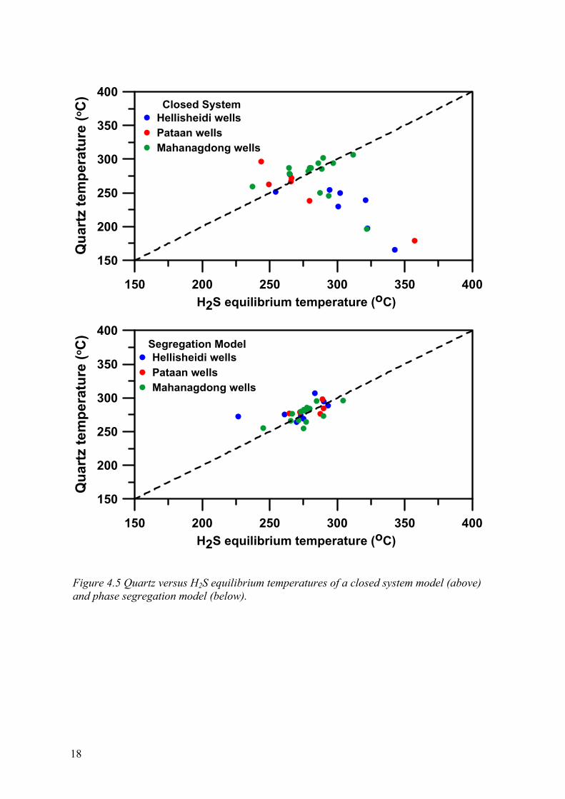
Figure 4.5 Quartz versus H2S equilibrium temperatures of a closed system model (above) and phase segregation model (below). ................................................ 18
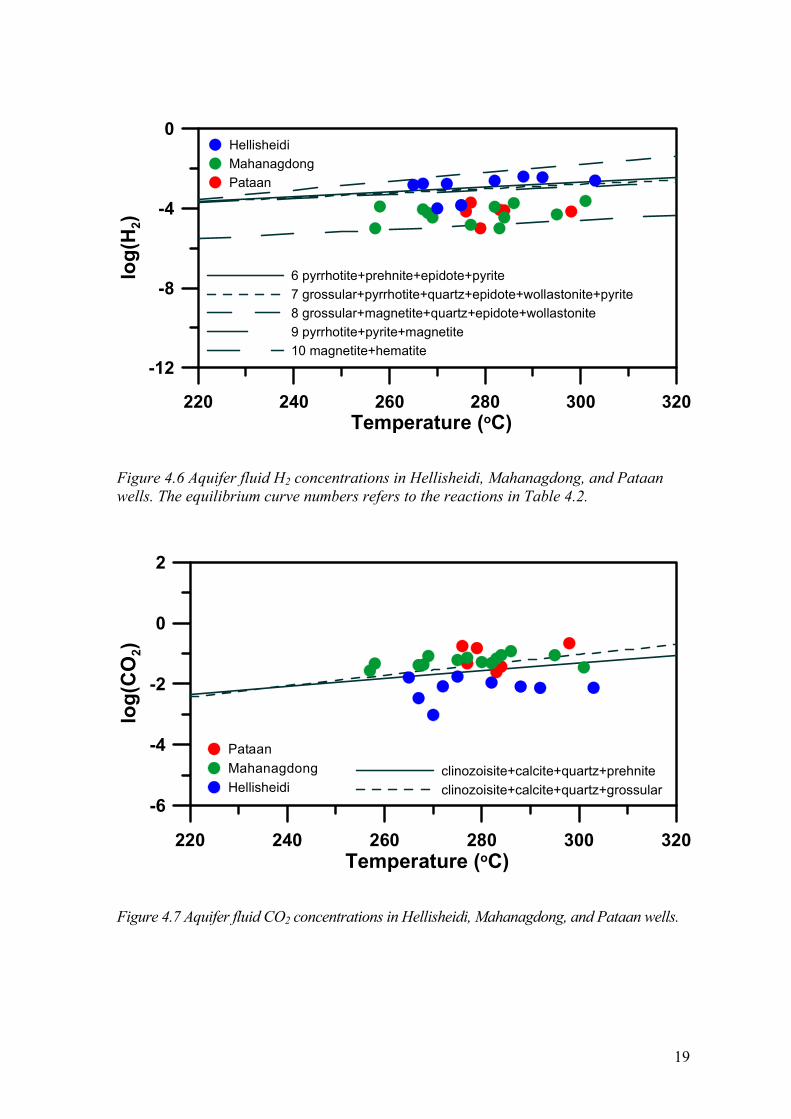
Figure 4.6 Aquifer fluid H2 concentrations in Hellisheidi, Mahanagdong, and Pataan wells. The equilibrium curve numbers refers to the reactions in Table 4.2. ...................................................................................................... 19
Figure 4.7 Aquifer fluid CO2 concentrations in Hellisheidi, Mahanagdong, and Pataan wells. ..................................................................................................... 19
Figure 5.1 Cl-HCO3-SO4 ternary diagram of waters from Hellisheidi, Mahanagdong and Pataan wells. ...................................................................... 22
Figure 5.2 Na-Cl-K ternary diagram of geothermal waters from Hellisheidi, Mahanagdong and Pataan wells. This shows partially equilibrated/mixed and fully equilibrated fluid discharges of the wells .................................................................................................................. 23
Figure 6.1 Calcite saturation index of aquifer fluid versus the selected aquifer temperature. ...................................................................................................... 27
Figure 6.2 Calcite saturation index of aquifer fluid versus total discharge enthalpies. ......................................................................................................... 28
xiii
Figure 6.3 Calcite saturation index versus pH of the aquifer fluid. ...................................... 29
Figure 6.4 Anhydrite saturation index of aquifer fluid versus the selected aquifer temperature. ...................................................................................................... 31
Figure 6.5 Aquifer fluid H2S and H2 molal ratios in relation to the equilibrium curve of pyrite-magnetite mineral assemblage. ................................................ 32
Figure 6.6 Aquifer fluid H2S and H2 molal ratios in relation to the equilibrium curve of pyrite-pyyrhotite mineral assemblage................................................. 32
Figure 6.7 Calcite saturation of well HE03 during adiabatic boiling at different degassing coefficients. ...................................................................................... 34
Figure 6.8 Calcite saturation of well HE05 during adiabatic boiling at different degassing coefficients. ...................................................................................... 34
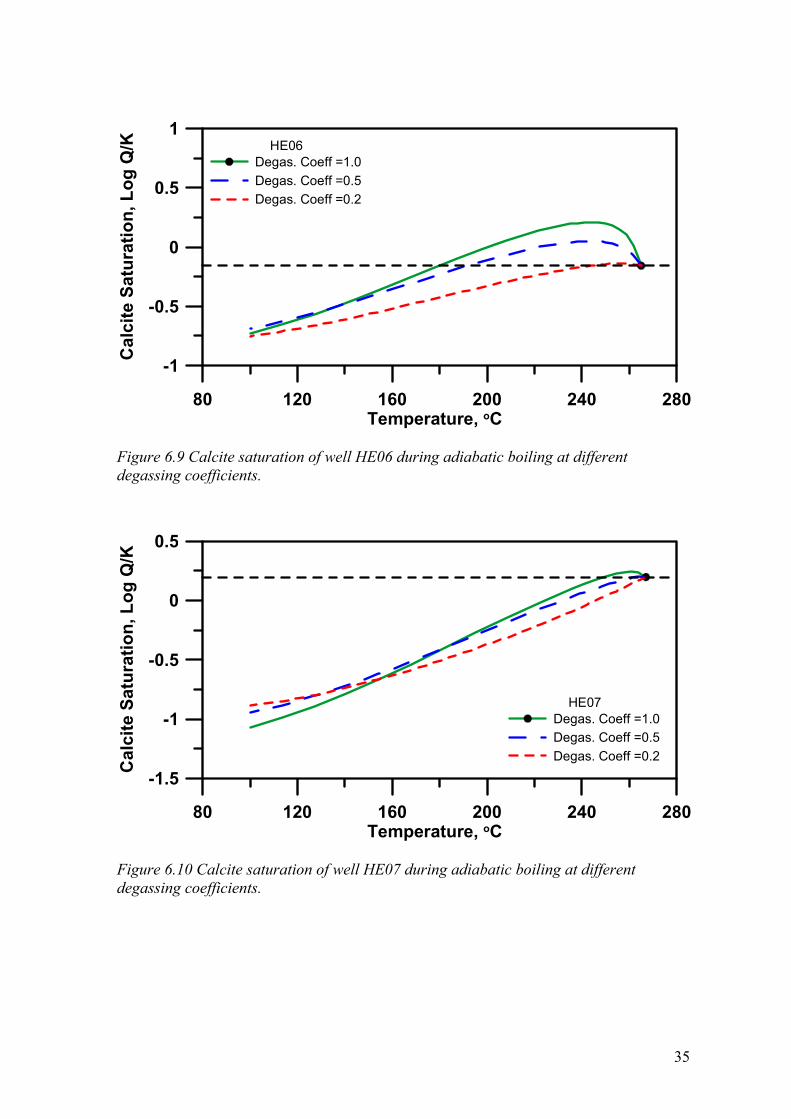
Figure 6.9 Calcite saturation of well HE06 during adiabatic boiling at different degassing coefficients. ...................................................................................... 35
Figure 6.10 Calcite saturation of well HE07 during adiabatic boiling at different degassing coefficients. ...................................................................................... 35
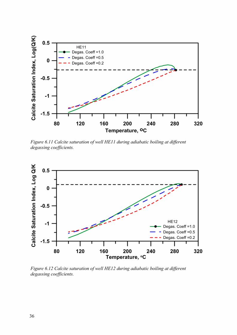
Figure 6.11 Calcite saturation of well HE11 during adiabatic boiling at different degassing coefficients. ...................................................................................... 36
Figure 6.12 Calcite saturation of well HE12 during adiabatic boiling at different degassing coefficients. ...................................................................................... 36
Figure 6.13 Calcite saturation of well HE17 during adiabatic boiling at different degassing coefficients. ...................................................................................... 37
Figure 6.14 Calcite saturation of well HE18 during adiabatic boiling at different degassing coefficients. ...................................................................................... 37
Figure 6.15 Calcite saturation of well HE29 during adiabatic boiling at different degassing coefficients. ...................................................................................... 38
Figure 6.16 Calcite saturation of well MG01 during adiabatic boiling at different degassing coefficients. ...................................................................................... 39
Figure 6.17 Calcite saturation of well MG01 during adiabatic boiling at different degassing coefficients. The chemistry data used in this plot is taken during fluid discharge testing (5-Nov-1994) of the well prior to production. ........................................................................................................ 39
Figure 6.18 Calcite saturation of well MG02 during adiabatic boiling at different degassing coefficients. ...................................................................................... 40
Figure 6.19 Calcite saturation of well MG03 during adiabatic boiling at different degassing coefficients. ...................................................................................... 40
xiv
Figure 6.20 Calcite saturation of well MG07 during adiabatic boiling at different degassing coefficients. ...................................................................................... 41
Figure 6.21 Calcite saturation of well MG13 during adiabatic boiling at different degassing coefficients. ...................................................................................... 41
Figure 6.22 Calcite saturation of well MG14 during adiabatic boiling at different degassing coefficients. ...................................................................................... 42
Figure 6.23 Calcite saturation of well MG16 during adiabatic boiling at different degassing coefficients. ...................................................................................... 42
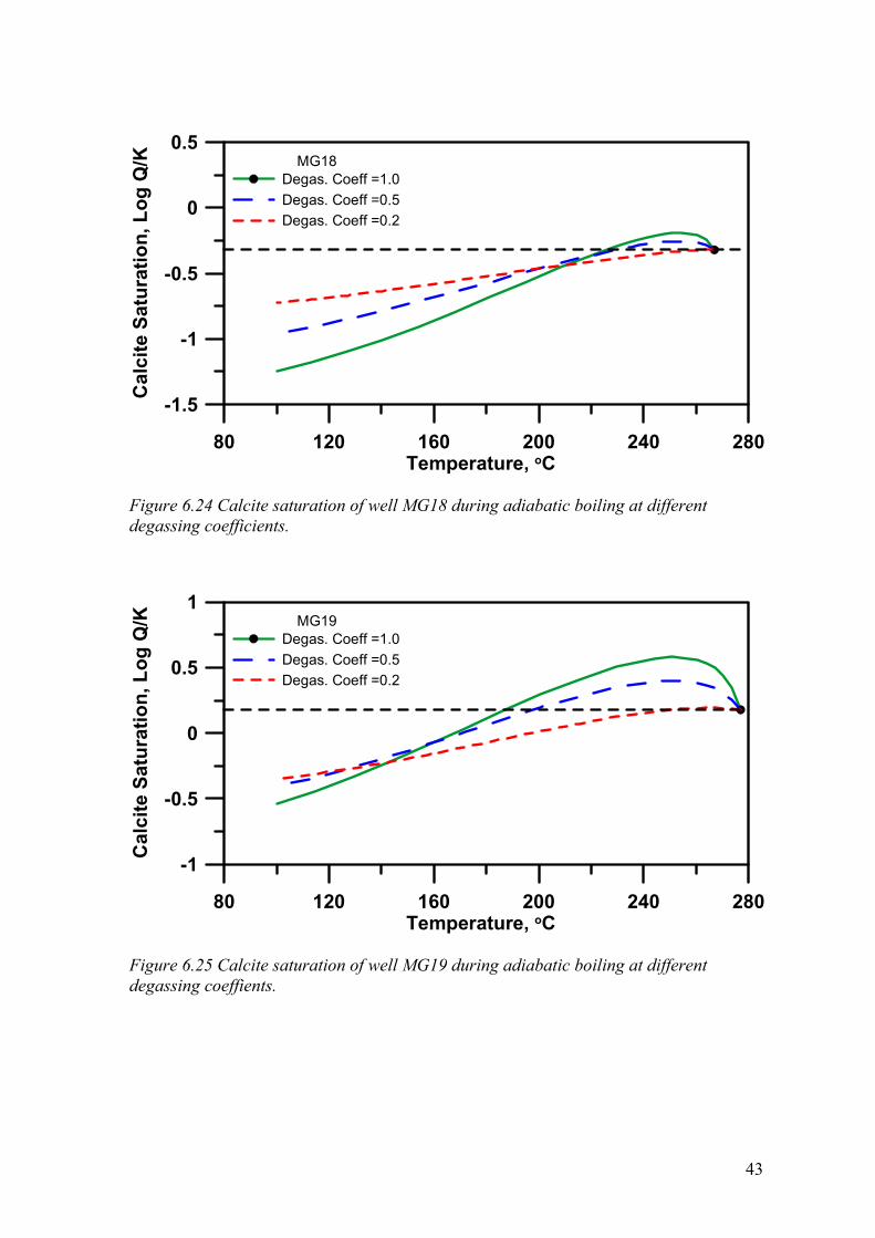
Figure 6.24 Calcite saturation of well MG18 during adiabatic boiling at different degassing coefficients. ...................................................................................... 43
Figure 6.25 Calcite saturation of well MG19 during adiabatic boiling at different degassing coeffients.......................................................................................... 43
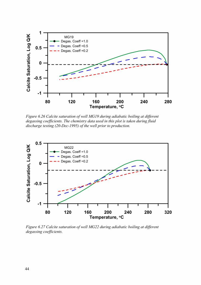
Figure 6.26 Calcite saturation of well MG19 during adiabatic boiling at different degassing coefficients. The chemistry data used in this plot is taken during fluid discharge testing (20-Dec-1995) of the well prior to production. ........................................................................................................ 44
Figure 6.27 Calcite saturation of well MG22 during adiabatic boiling at different degassing coefficients. ...................................................................................... 44
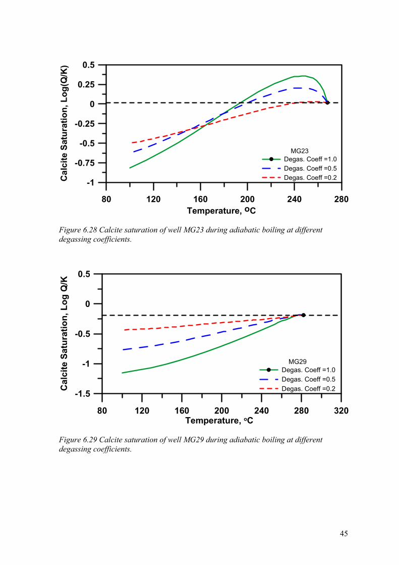
Figure 6.28 Calcite saturation of well MG23 during adiabatic boiling at different degassing coefficients. ...................................................................................... 45
Figure 6.29 Calcite saturation of well MG29 during adiabatic boiling at different degassing coefficients. ...................................................................................... 45
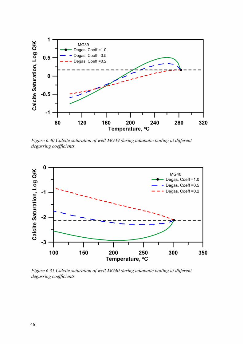
Figure 6.30 Calcite saturation of well MG39 during adiabatic boiling at different degassing coefficients. ...................................................................................... 46
Figure 6.31 Calcite saturation of well MG40 during adiabatic boiling at different degassing coefficients. ...................................................................................... 46
Figure 6.32 Inferred fluid flow paths at Mahanagdong geothermal field. Based on Salonga et al ( 2004). ................................................................................... 47
Figure 6.33 Calcite saturation of well PT02 during adiabatic boiling at different degassing coefficients. ...................................................................................... 48
Figure 6.34 Calcite saturation of well PT04 during adiabatic boiling at different degassing coefficients. ...................................................................................... 49
Figure 6.35 Calcite saturation of well PT05 during adiabatic boiling at different degassing coefficients. ...................................................................................... 49
Figure 6.36 Calcite saturation of well PT07 during adiabatic boiling at different degassing coefficients. ...................................................................................... 50
xv
Figure 6.37 Calcite saturation of well PT08 during adiabatic boiling at different degassing coefficients. ...................................................................................... 50
Figure 6.38 Calcite saturation of well PT10 during adiabatic boiling at different degassing coefficients. ...................................................................................... 51
Figure 6.39 Pataan well tracks and the inferred temperature contour based on quartz geothermometer using closed system model in 2007 resource assessment. The dash line refers to the slotted liner of the well which is open for production. Modified after Olivar, 2007. ........................................ 51
Figure 6.40 Natural stable reservoir pressure of different Philippine geothermal fields. Pataan wells are located in Northen Negros, Philippines. BACMAN refers to Bacon-Manito and SNGPF refers to Southern Negros Geothermal Production Fields. Reprint from Olivar, 2007. ................. 52
Figure 6.41 Total discharge enthalpy and mass flow of Pataan wells before and during commissioning in 2007. Reprint from Olivar (2007). ........................... 52
Figure 6.42 Calcite saturation of well MD01 during adiabatic boiling at different degassing coefficients. ...................................................................................... 53
Figure 6.43 Calcite saturation of mixed fluids of well HE03 during adiabatic boiling at equilibrium degassing. ...................................................................... 54
Figure 6.44 Calcite saturation of mixed fluids of well HE05 during adiabatic boiling at equilibrium degassing. ...................................................................... 55
Figure 6.45 Calcite saturation of mixed fluids of well HE06 during adiabatic boiling at equilibrium degassing. ...................................................................... 55
Figure 6.46 Calcite saturation of mixed fluids of well HE07 during adiabatic boiling at equilibrium degassing. ...................................................................... 56
Figure 6.47 Calcite saturation of mixed fluids of well HE11 during adiabatic boiling at equilibrium degassing. ...................................................................... 56
Figure 6.48 Calcite saturation of mixed fluids of well HE12 during adiabatic boiling at equilibrium degassing. ...................................................................... 57
Figure 6.49 Calcite saturation of mixed fluids of well HE17 during adiabatic boiling at equilibrium degassing. ...................................................................... 57
Figure 6.50 Calcite saturation of mixed fluids of well HE18 during adiabatic boiling at equilibrium degassing. ...................................................................... 58
Figure 6.51 Calcite saturation of mixed fluids of well HE29 during adiabatic boiling at equilibrium degassing. ...................................................................... 58
Figure 6.52 Calcite saturation of mixed fluids of well PT02 during adiabatic boiling at equilibrium degassing. ...................................................................... 59
xvi
Figure 6.53 Calcite saturation of mixed fluids of well PT04 during adiabatic boiling at equilibrium degassing. ..................................................................... 59
Figure 6.54 Calcite saturation of mixed fluids of well PT05 during adiabatic boiling at equilibrium degassing. ..................................................................... 60
Figure 6.55 Calcite saturation of mixed fluids of well PT07 during adiabatic boiling at equilibrium degassing. ..................................................................... 60
Figure 6.56 Calcite saturation of mixed fluids of well PT08 during adiabatic boiling at equilibrium degassing. ..................................................................... 61
Figure 6.57 Calcite saturation of mixed fluids of well PT10 during adiabatic boiling at equilibrium degassing. ..................................................................... 61
xvii
List of Tables Table 3.1 Measured discharge enthalpies and separated water analyses of well
fluid discharges. ..................................................................................................... 9
Table 3.2 Separated gas analyses of the well fluid discharges. ........................................... 10
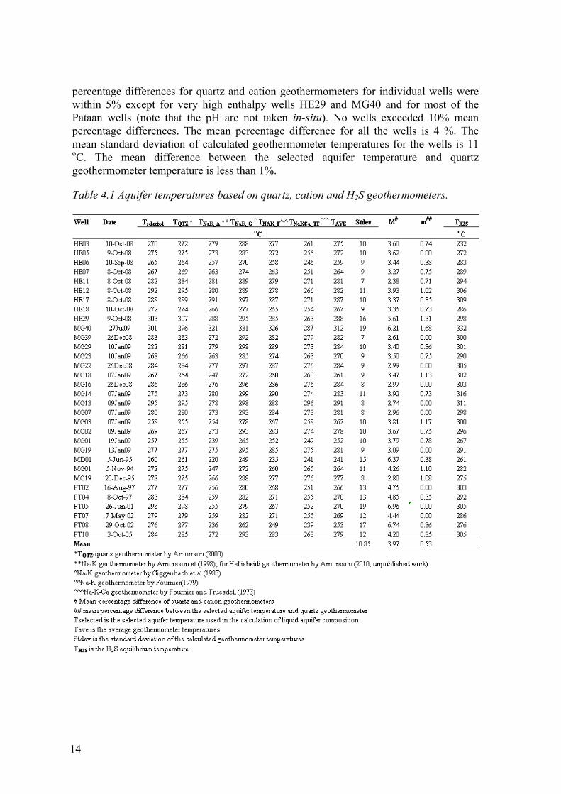
Table 4.1 Aquifer temperatures based on quartz, cation and H2S geothermometers. ................................................................................................. 14
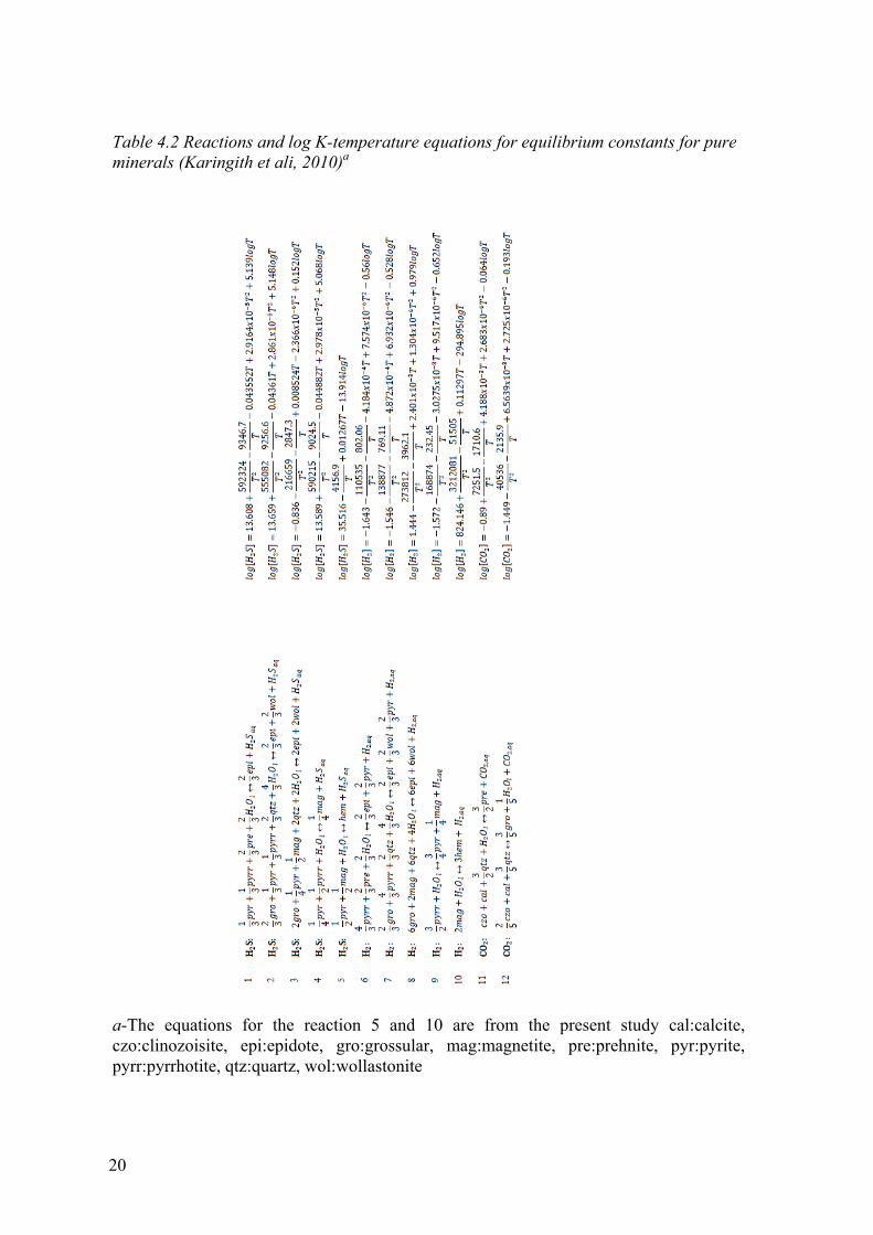
Table 4.2 Reactions and log K-temperature equations for equilibrium constants for pure minerals (Karingith et ali, 2010)a ........................................................... 20
Table 5.1 Aquifer fluid composition based on the phase segregation model. ..................... 21
Table 6.1 Log K-temperature equations of individual mineral dissolution reactions (valid at 0-350°C at Psat, unit activity for all minerals and liquid water) modified after Angcoy (2010). ....................................................... 30
Table 6.2 Mixed brine chemistry of Hellisheidi and Pataan wells. ..................................... 53
Table 6.3 Compositions of mixed fluids ( aquifer fluid and injected mixed brine) of Hellisheidi wells based on PHREEQC simulations. ....................................... 62
Table 6.4 Compositions of mixed fluids ( aquifer fluid and injected mixed brine) of Pataan wells based on PHREEQC simulations. .............................................. 63

xix
Acknowledgements I would like to extend my great appreciation and deepest gratitude to…
Edda Lilja Sveinsdóttir and REYST Academic Council for giving me a chance to finish my research work despite my rather complicated situation. Special thanks to Edda Lilja for all the administrative and moral support that she unconditionally gave me.
Orkuveita Reykjavikur (Reykjavik Energy) through Einar Gunnlaugsson for funding my research work.
Ingvi Gunnarsson of Reykjavik Energy who helped in well sampling and laboratory analyses.
Prof. Behdad Moghtaderi and Elham Doroodchi of Priority Reseach Centre for Energy, The University of Newcastle, Australia, for giving considerations and allowing me to take leave of absence to finish my research in Iceland.
The management and staff of Energy Development Corporation. Special mention to Marivic Olivar for providing the Pataan well data and Erlindo C. Angcoy for providing the Mahanagdong well data as well as their indirect help through their publications and reports.
The first batch of REYST students who have been warm and accommodating and made my stay in Iceland uniquely memorable. They have been great in providing all kinds of support (moral, technical, etc.).
My supervisor, Prof. Stefan Arnórsson, not only for his useful advice but also for his patience and very kind consideration. Without his understanding and consideration, I would not have the chance to finish this research.

1
1 Introduction Numerous studies on the effect of calcite formation on the operation of geothermal power plants and facilities have been published since the utilization of geothermal resources for power generation and space heating (Arnórsson, 1978, Arnórsson, 1989, Rahmani, 2007, Satman et al., 1999, Siega et al., 2005, Stáhl et al., 2000, Sanchez et al., 2005 and many others).
It is commonly known that precipitation of calcium carbonate minerals (mostly calcite and rare aragonite) is enhanced by depressurization boiling and controlled by the reaction
Ca++ + 2HCO3- = CaCO3(s) + H2O + CO2 (aq) or Ca++ + 2HCO3
- = CaCO3(s) + H2CO3 (1)
(Sanchez et al., 2005, Satman et al., 1999, Siega et al., 2005). Ultimately, however, the potential for precipitation and scaling are dependent on saturation of the initial aquifer fluid and the processes it will undergo like boiling, phase segregation, mixing, and others (Arnorsson et al., 2007).
This thesis will do comparative studies and assess the calcite precipitation potential of geothermal fluids from some of the Hengill-Hellisheidi geothermal wells in Iceland, Pataan wells in Northern Negros, Philippines and Mahanagdong wells in Leyte, Philippines.
Wells that are suspected and/or have been known to be affected by calcite scale formation are wells from Pataan and wells MG01 and MG19 from Mahanagdong. One well from Mindanao Geothermal Production Field, MD01, is also included in the pool of well data.
There are two sets of data for wells MG01 and MG19—one set is from Angcoy (2010) and the other set is from Olivar (personal comm.) which was taken before commercial production in the area. They are compared for changes in the aquifer fluid and calcite saturation after 15 years of production.

2
3
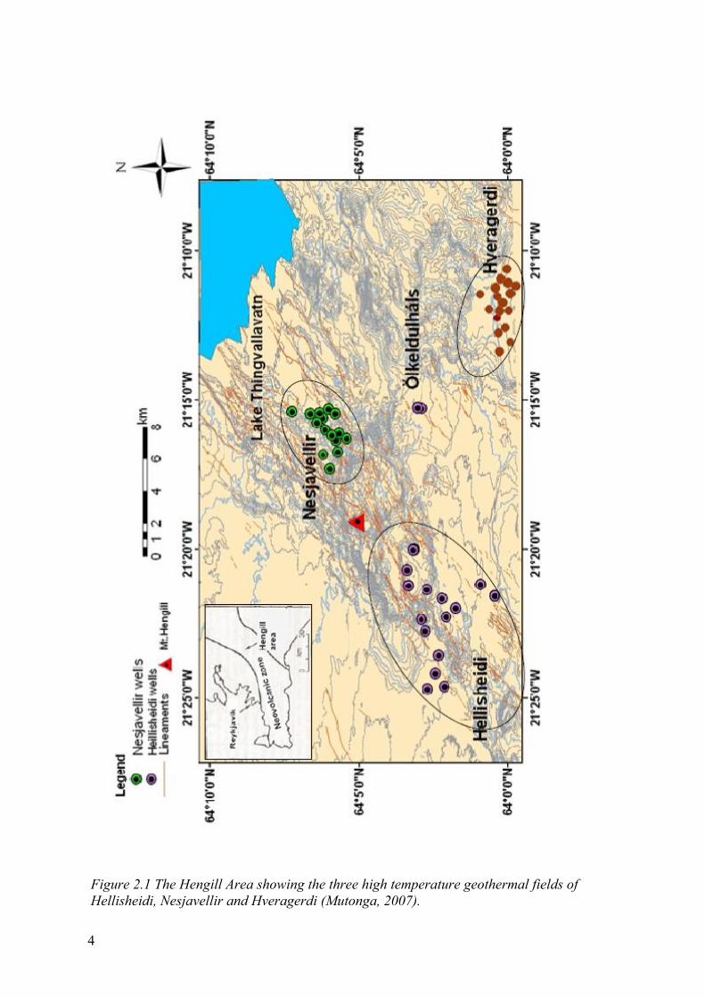
2 Geothermal Fields Hellisheidi is a high-temperature geothermal field located in the southern sector of the Hengill central volcano in SW Iceland. It is part of the Hengill area which contains three geothermal fields, including the Nesjavellir and Hveragerdi geothermal fields, Figure 2.1 (Bjornsson et al., 2003, Franzson et al., 2005, Mutonga, 2007, Bjornsson, 2004 and many others). Geothermal systems in Iceland were classified by Bödvarsson (1961) as high and low-temperature. They have been described by Arnorsson (1995b and 1995a). Chemistry of geothermal waters in Iceland has been reported by several authors (Arnorsson, 1979, Arnórsson, 1983, Arnórsson et al., 1978, Arnórsson et al., 1983a, Arnórsson et al., 1983b, Gudmundsson and Arnórsson, 2005, Stefánsson and Arnórsson, 2002).
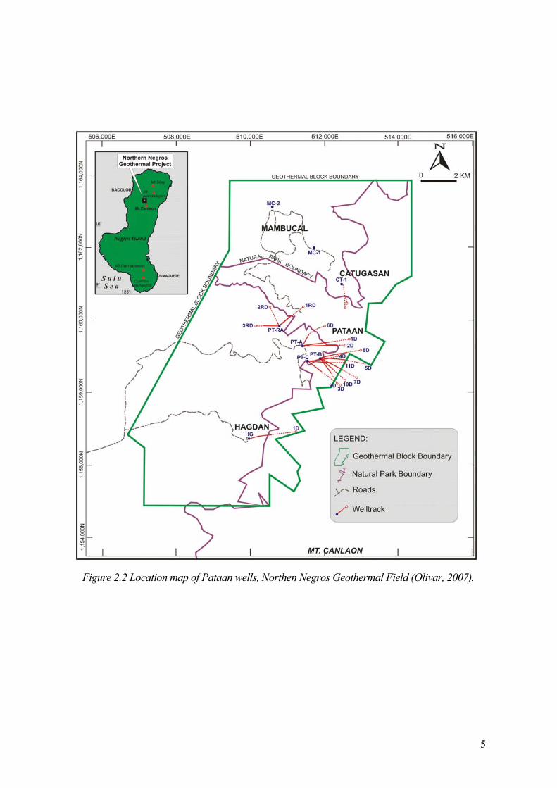
Pataan geothermal wells are situated in the northern part of the Negros Island in central Philippines and are part of the Northern Negros Geothermal Field (Figure 2.2). A total of 11 wells were drilled in the area, five of which have not been used for production (Olivar, 2007).
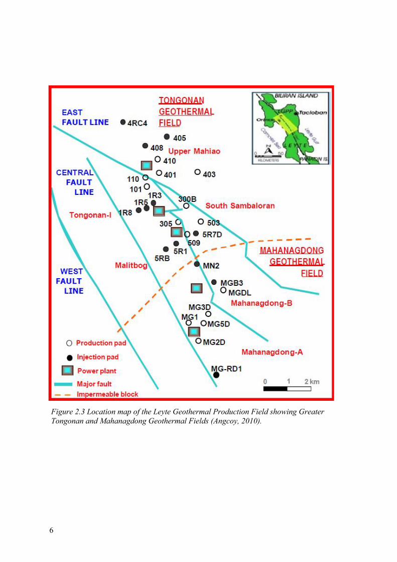
Mahanagdong is located in the southern part of the Greater Tongonan Geothermal Field in the island of Leyte, Philippines (Figure 2.3). This geothermal field is widely studied, as cited by Angcoy (2010) from exploration to exploitation and monitoring.
The wells from these geothermal fields should represent the varying characteristics of geothermal fluid discharges in different geological settings, ranging in composition from dilute to high salinities, and from different host rocks, i.e. basaltic and andesitic.
4
Figure 2.1 The Hengill Area showing the three high temperature geothermal fields of Hellisheidi, Nesjavellir and Hveragerdi (Mutonga, 2007).
5
Figure 2.2 Location map of Pataan wells, Northen Negros Geothermal Field (Olivar, 2007).
6
Figure 2.3 Location map of the Leyte Geothermal Production Field showing Greater Tongonan and Mahanagdong Geothermal Fields (Angcoy, 2010).
7
3 Sampling and Analysis
3.1 Collection of Water and Steam Samples from Wet-Steam Wells
Comprehensive water and gas sampling techniques for geothermal wells have been described by Arnorsson et al (2006) and references therein.
Webre-separator installed at the two-phase line near the wellhead was used to separate and collect steam and liquid water samples at the same sampling pressure. It was ensured that the vapor coming out of the steam outlet was dry before collecting using pre-evacuated gas bulbs.
Steam samples were collected using double-ended gas bulbs. A pre-weighed and evacuated gas bulb containing 35% NaOH solution was used to collect steam samples from the Philippine fields for non-condensible (CO2 and H2S are captured by the strong base) and residual gases (H2, CH4, Ar and N2 occupied the head space) analyses. In the case of Hellisheidi wells, 50% v/w KOH solution was used instead of 35% NaOH. For Mahanagdong and Pataan, another gas bulb was used for collection of steam condensate for water-soluble NH3 analysis.
CO2 and H2S in the hydroxide solution were analyzed by titration while the residual gases in the head space of the gas sampling bulbs were analyzed on a gas-chromatograph. NH3 in the steam condensate was analyzed by ion-selective electrode method (Pataan and Mahanagdong wells). At Hellisheidi, CO2 was also determined by ion chromatography.
Liquid water samples collected from the webre-separator were cooled in a stainless steel cooling coil submerged in a water bath. Generally, there were three sets of liquid water samples collected for each well depending on the sample treatments. They were filtered and air-free, filtered and acidified (5ml HNO3 to 1000 ml sample for Mahanagdong and Pataan, 0.5ml 5ml HNO3 to 1000 ml sample for Hellisheidi), and unfiltered and air-free.
For Hellisheidi and Mahanagdong wells, liquid water analyses pertinent to these studies included 1) on-site determination pH, H2S and total carbonate carbon and 2) analysis of major elements and some minor and trace elements using Spectro CirosTM Inductively Coupled Plasma-Atomic Emission Spectrometer (ICP-AES) and Reagent Free Ion Chromatograph (RFICTM, Dionex 2000). Water analyses of Pataan wells were based from EDC laboratory procedures manual (Angcoy, 2010) which include: 1) pH by electrometric method, 2) total carbonate carbon by titration, 3) H2S by iodometry, 4) Cl by argentometric-potentiometric method, 5) total SiO2 by spectrophotometry (heteropoly blue), 6) metals (Na, K, Ca, Mg, Fe, Li) by Atomic Absorption Spectrometry (AAS), 7) B by titrimetry (mannitol) and 8) SO4
-2 by colorimetry (barium chromate/bromophenol blue).
8
The effect of silica polymerization on pH was reported by Gunnarsson and Arnórsson (2005) and therefore expected to have differences between in-situ pH measurement and laboratory result if considerable time has elapsed before measurement. The magnitude of pH differences are dependent on the weak-acids and buffers present in the fluid (Angcoy, 2010, Zhong-He and Ármansson, 2006). The comparison showed that on-site pH measurement is systematically lower by about 0.2 pH units compared with laboratory measurements for the case of Mahanagdong geothermal wells (Angcoy, 2010). The difference is considerably higher for the Hellisheidi wells.
3.2 Analytical Results
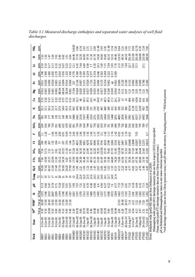
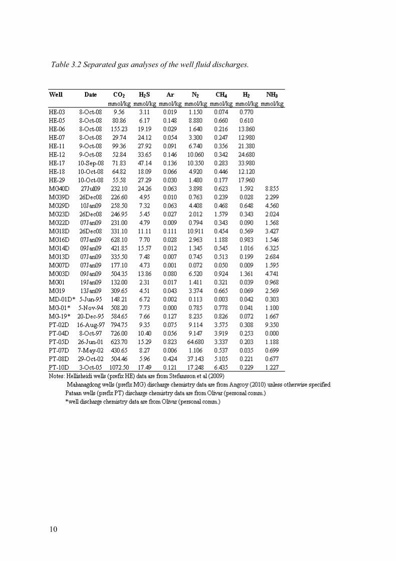
Measured discharge enthalpies and analyses of separated water from Hellisheidi, Pataan, and Mahanagdong geothermal wells are listed in Table 3.1. Separated gas analyses are listed in Table 3.2. Water and gas analyses from Hellisheidi geothermal wells are from Stefansson et al (2009), Mahanagdong wells are from Angcoy (2010) and Pataan wells are from Olivar (personal comm.). It should be noted that the separated water pH measurement from Hellisheidi and Mahanagdong wells were done on-site and pH from Pataan were measured in the laboratory. Also, water and gas samples from Hellisheidi and Mahanagdong were taken during normal production discharges of the wells whereas Pataan water and gas samples were taken before commercial production or during discharge testing of the wells.
Separated water from Hellisheidi wells are highly alkaline (8.47-9.24) while that from Pataan and Mahanagdong are slightly acidic to near-neutral. Pataan has the most saline separated water >10,000 ppm Cl, Hellisheidi has diluted water with < 500 ppm Cl and Mahanagdong in the middle with 2,000<Cl< 7,500 ppm. Dissolved H2S is high in Hellisheidi (20 – 80 ppm) compared to Mahanagdong (0.3 -2.7 ppm) and Pataan (2-10 ppm). However, dissolved CO2 in Hellisheidi (4-35 ppm) is lowest compared to Mahanagdong (17-74 ppm) and Pataan (30-68 ppm). Ca2+ concentrations in Pataan are high ranging from 490 -1050 ppm compared to Mahanagdong (8-216 ppm) and Hellisheidi (< 1 ppm)
Separated vapour from Pataan wells has the highest CO2 concentration (431-1073 mmol/kg) while Hellisheidi has the lowest concentration (10-155 mmol/kg) and Mahanagdong at the middle (132-628 mmol/kg). Hellisheidi has high H2 gas concentration (up to 34 mmol/kg) compared to Mahanagdong (< 2 mmol/kg) and Pataan (<1 mmol/kg).
9
Table 3.1 Measured discharge enthalpies and separated water analyses of well fluid discharges.
10
Table 3.2 Separated gas analyses of the well fluid discharges.
11
4 Data Handling Separated water and gas analyses from the wells are used to infer aquifer fluid compositions with the help of a speciation program WATCH developed by Arnosson et al (1982), version 2.1 (Bjarnason, 1994).
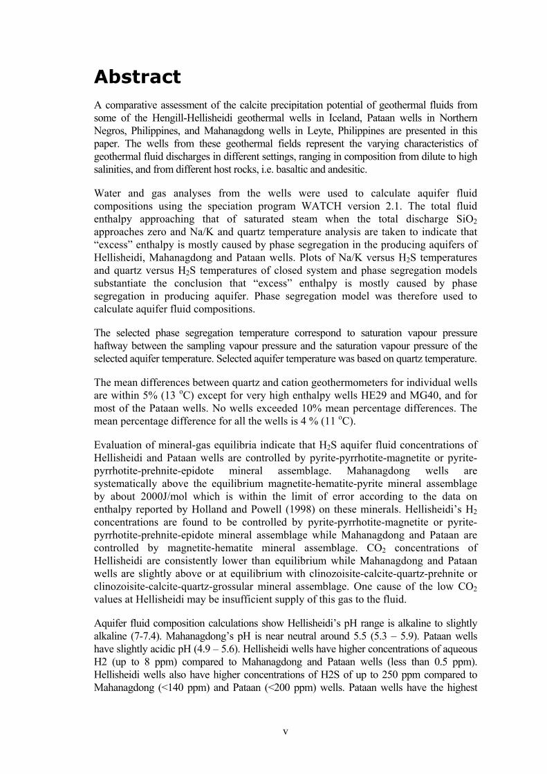
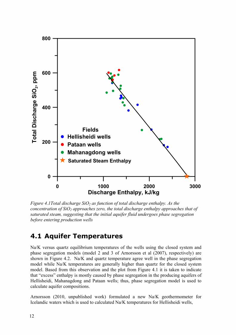
Several models of boiling and phase segregation of aquifer fluid have been postulated to explain “excess discharge enthalpy of a geothermal well (Arnorsson et al., 2007). Plot of SiO2 versus discharge enthalpy is shown in Figure 4.1 for all the wells considered in this study. If the aquifer temperature is fairly constant, the plot showing discharge enthalpy approaching that of saturated steam when SiO2 approaches zero indicates that the excess discharge enthalpy can be explained by phase segregation rather than conductive heating of the fluid by host rock (Arnorsson et al., 2007). The use of geothermometers to validate phase segregation model are discussed in the succeeding sections.
In phase segregation model, one has to choose the temperature at which water and steam segregate. In this study, the phase segregation temperature is calculated as the saturation temperature of the phase segregation vapour pressure. Segregation pressure is calculated as the midpoint between the sampling pressure and the saturation vapour pressure of the selected aquifer temperature. Selected aquifer temperature is based on quartz solubility data according to Gunnarsson and Arnorsson (2000). The procedure is somewhat iterative as one is to assume first the aquifer temperature then check if one will get comparable quartz geothermometer temperature from the calculated aquifer fluid composition. One must then adjust the selected aquifer temperature appropriately and calculate for the new segregation pressure until the selected aquifer temperature equals quartz geothermometer temperature.
The calculation of the aquifer fluid composition was done in two-step run by the speciation program WATCH. Separated water and gas analyses, measured discharge enthalpy and measured pH were used in the first WATCH run which use arbitrary reference temperature equal to the segregation temperature.
The output of the first WATCH run was then used as input in the second WATCH run. The segregation pressure was set as the sampling pressure and pH was the output from the first run with the corresponding temperature equal to the segregation temperature. Flowing fluid enthalpy was set to liquid enthalpy at the selected aquifer temperature. The model reference temperature was then set to the selected aquifer temperature. The output of the second WATCH run is the calculated aquifer fluid composition assuming liquid enthalpy at the aquifer.
Fluid mixing of the aquifer fluids with injected mixed brine will be simulated using geochemical model PHREEQC (Parkhurst and Appelo, 1999) using the graphical windows interface developed by Vincent Post (http://www.falw.vu/~ posv/ phreeqc/index.html). The mixed fluid is then inputted into WATCH for simulations of boiling and degassing.
12
0 1000 2000 3000Discharge Enthalpy, kJ/kg
0
200
400
600
800To
tal D
isch
arge
SiO
2, pp
m
FieldsHellisheidi wellsPataan wellsMahanagdong wellsSaturated Steam Enthalpy
Figure 4.1Total discharge SiO2 as function of total discharge enthalpy. As the concentration of SiO2 approaches zero, the total discharge enthalpy approaches that of saturated steam, suggesting that the initial aquifer fluid undergoes phase segregation before entering production wells
4.1 Aquifer Temperatures
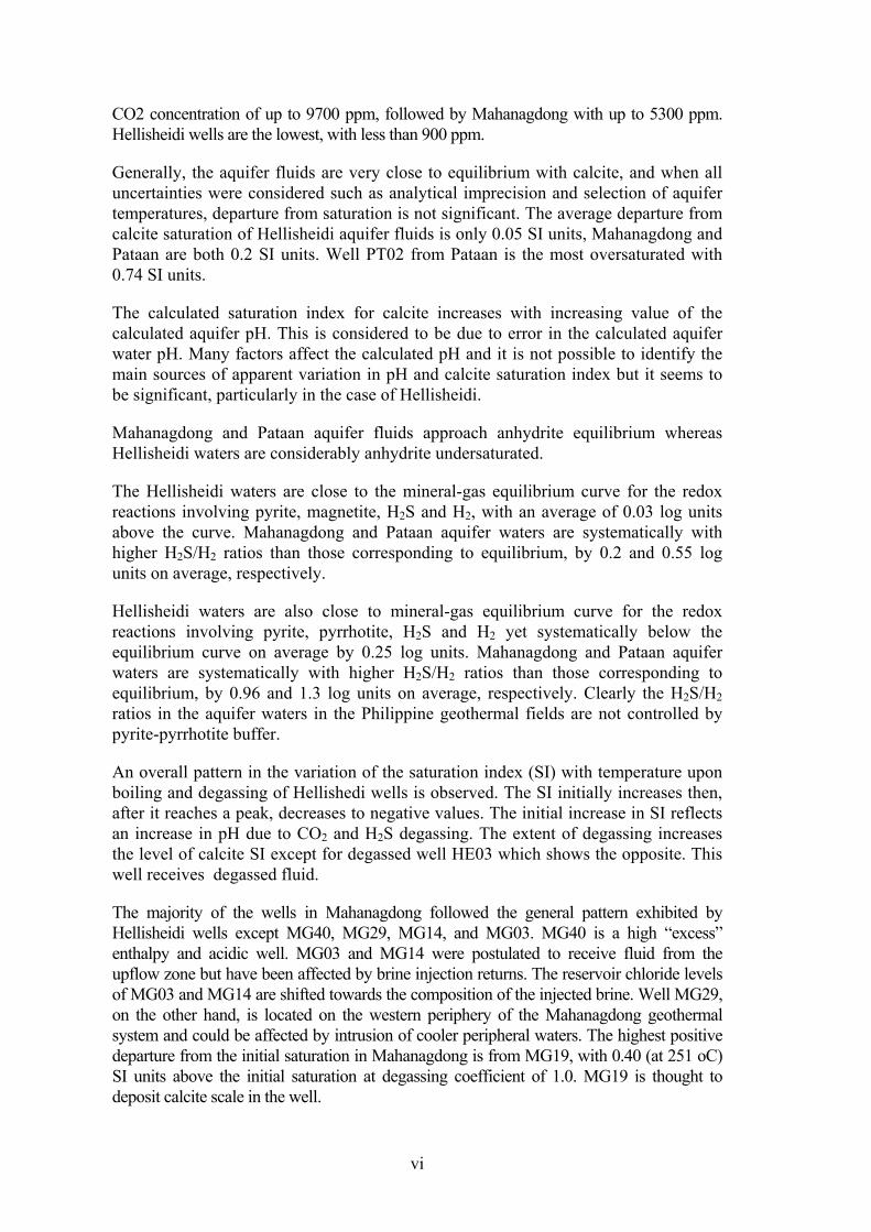
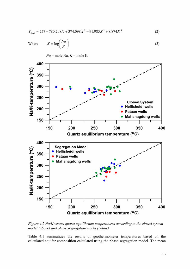
Na/K versus quartz equilibrium temperatures of the wells using the closed system and phase segregation models (model 2 and 3 of Arnorsson et al (2007), respectively) are shown in Figure 4.2. Na/K and quartz temperature agree well in the phase segregation model while Na/K temperatures are generally higher than quartz for the closed system model. Based from this observation and the plot from Figure 4.1 it is taken to indicate that “excess” enthalpy is mostly caused by phase segregation in the producing aquifers of Hellisheidi, Mahanagdong and Pataan wells; thus, phase segregation model is used to calculate aquifer compositions.
Arnorsson (2010, unpublished work) formulated a new Na/K geothermometer for Icelandic waters which is used to calculated Na/K temperatures for Hellisheidi wells,
13
432 874.8985.91098.374208.780757 XXXXTNaK +−+−= (2)
Where ⎟⎠⎞
⎜⎝⎛=
KNaX log (3)
Na = mole Na, K = mole K
150 200 250 300 350 400Quartz equilibrium temperature (oC)
150
200
250
300
350
400
Na/
K-te
mpe
ratu
re (o C
) Segregation ModelHellisheidi wellsPataan wellsMahanagdong wells
150 200 250 300 350 400Quartz equilibrium temperature (oC)
150
200
250
300
350
400
Na/
K-te
mpe
ratu
re (o C
)
Closed SystemHellisheidi wellsPataan wellsMahanagdong wells
Figure 4.2 Na/K versus quartz equilibrium temperatures according to the closed system model (above) and phase segregation model (below).
Table 4.1 summarizes the results of geothermometer temperatures based on the calculated aquifer composition calculated using the phase segregation model. The mean
14
percentage differences for quartz and cation geothermometers for individual wells were within 5% except for very high enthalpy wells HE29 and MG40 and for most of the Pataan wells (note that the pH are not taken in-situ). No wells exceeded 10% mean percentage differences. The mean percentage difference for all the wells is 4 %. The mean standard deviation of calculated geothermometer temperatures for the wells is 11 oC. The mean difference between the selected aquifer temperature and quartz geothermometer temperature is less than 1%.
Table 4.1 Aquifer temperatures based on quartz, cation and H2S geothermometers.
15
4.2 Mineral Assemblage-H2S Equilibria
Equilibrium constants derived by Arnórsson et al. (2010), as cited by Angcoy (2010), for several mineral assemblages that potentially could control the concentrations of H2S, H2 and CO2 in the aquifer fluid are listed in Table 4.2. Also shown in Table 4.2 are the respective reactions and temperature equations for the equilibrium constants. The equilibrium constants were derived from thermodynamic data on oxide and silicate minerals as given by Holland and Powell (1998), but those on pyrite and pyrrhotite minerals by Robie and Hemmingway (1995). Data on the dissolved gases were retrieved from data on Henry’s Law coefficients given by Fernandez-Prini et al (2003) and the pure gases according to Robie and Hemingway (1995).
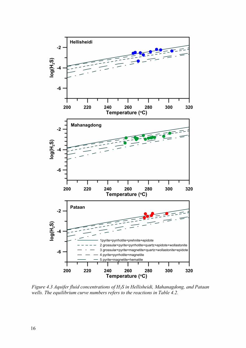
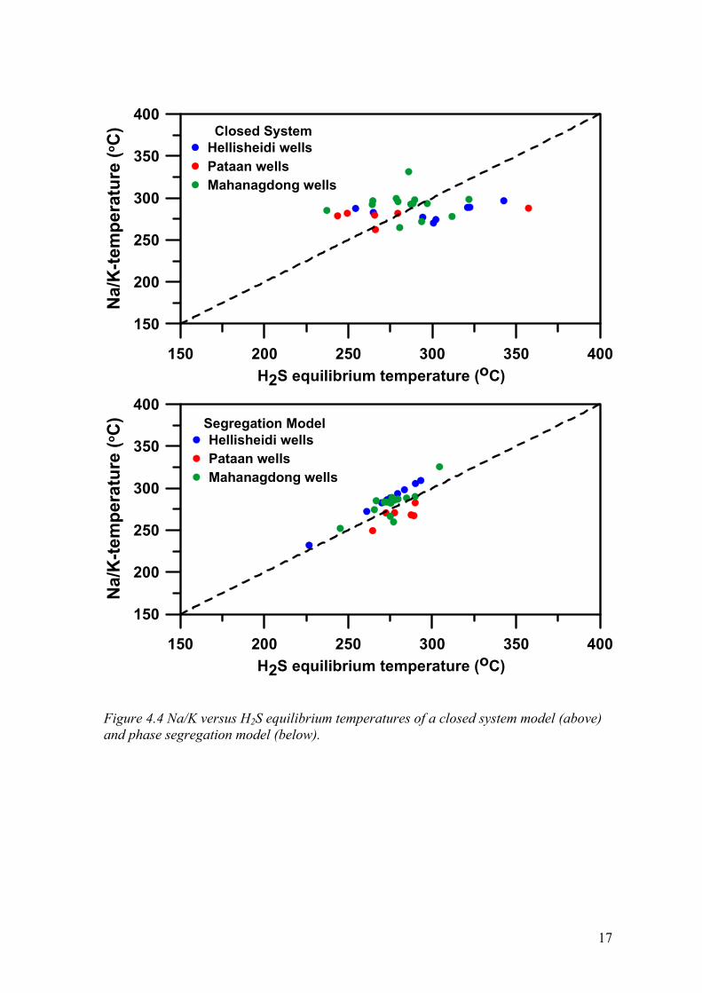
Figure 4.3 shows the concentrations of H2S as plotted against equilibrium reaction curves that could potentially control its concentration in the aquifer fluid. H2S aquifer fluid concentrations of Hellisheidi and Pataan wells are controlled by pyrite-pyrrhotite-magnetite mineral assemblage (reaction 4 in Table 4.2). One well from Hellisheidi (HE03) was significantly below the curve but was found to be highly degassed. Hellisheidi aqueous H2S concentrations can also be controlled by pyrite-pyrrhotite-prehnite-epidote mineral assemblage (reaction 1). The data points of Mahanagdong wells are systematically above the equilibrium magnetite-hematite-pyrite mineral assemblage (reaction 5), by about 2000J/mol. According to the data on enthalpy reported by Holland and Powell (1998) on these minerals, it is within the limit of error. Temperatures have been calculated for the two H2S mineral equilibria in Table 4. Na/K versus H2S temperatures and quartz versus H2S temperatures of closed system and phase segregation models were plotted in Figures 4.4 and 4.5, respectively. Both plots show scattered data for closed system model. It also show, however, that H2S temperatures are systematically higher than quartz temperatures on the phase segregation model but they agree well nonetheless. The results for the three areas substantiate the conclusion that “excess” enthalpy is mostly caused by phase segregation in producing aquifer.
H2 aquifer fluid concentrations of all wells are plotted in Figure 4.6. Hellisheidi’s H2 aquifer fluid concentrations are controlled by pyrite-pyrrhotite-magnetite (reaction 9) or pyrite-pyrrhotite-prehnite-epidote (reaction 6) mineral assemblage. Mahanagdong and Pataan H2 aquifer fluid concentrations on the other hand are controlled by magnetite-hematite mineral assemblage (reaction 10).
Hellisheidi CO2 concentrations are consistently lower than equilibrium while Mahanagdong wells are slightly above or at equilibrium with the mineral assemblage clinozoisite-calcite-quartz-prehnite or clinozoisite-calcite-quartz-grossular (Figure 4.7). One cause of the low CO2 values at Hellisheidi may be insufficient supply of this gas to the fluid.
16
200 220 240 260 280 300 320Temperature (oC)
-6
-4
-2
log(
H2S
)
200 220 240 260 280 300 320Temperature (oC)
-6
-4
-2
log(
H2S
)
200 220 240 260 280 300 320Temperature (oC)
-6
-4
-2lo
g(H
2S)
1pyrite+pyrrhotite+prehnite+epidote2 grossular+pyrite+pyrrhotite+quartz+epidote+wollastonite3 grossular+pyrite+magnetite+quartz+wollastonite+epidote4 pyrite+pyrrhotite+magnetite5 pyrite+magnetite+hematite
Hellisheidi
Mahanagdong
Pataan
Figure 4.3 Aquifer fluid concentrations of H2S in Hellisheidi, Mahanagdong, and Pataan wells. The equilibrium curve numbers refers to the reactions in Table 4.2.
17
150 200 250 300 350 400H2S equilibrium temperature (oC)
150
200
250
300
350
400
Na/
K-te
mpe
ratu
re (o C
) Segregation ModelHellisheidi wellsPataan wellsMahanagdong wells
150 200 250 300 350 400H2S equilibrium temperature (oC)
150
200
250
300
350
400N
a/K
-tem
pera
ture
(o C) Closed System
Hellisheidi wellsPataan wellsMahanagdong wells
Figure 4.4 Na/K versus H2S equilibrium temperatures of a closed system model (above) and phase segregation model (below).
18
150 200 250 300 350 400H2S equilibrium temperature (oC)
150
200
250
300
350
400
Qua
rtz
tem
pera
ture
(o C)
Segregation ModelHellisheidi wellsPataan wellsMahanagdong wells
150 200 250 300 350 400H2S equilibrium temperature (oC)
150
200
250
300
350
400Q
uart
z te
mpe
ratu
re (o C
) Closed SystemHellisheidi wellsPataan wellsMahanagdong wells
Figure 4.5 Quartz versus H2S equilibrium temperatures of a closed system model (above) and phase segregation model (below).
19
220 240 260 280 300 320Temperature (oC)
-12
-8
-4
0lo
g(H
2)
6 pyrrhotite+prehnite+epidote+pyrite7 grossular+pyrrhotite+quartz+epidote+wollastonite+pyrite8 grossular+magnetite+quartz+epidote+wollastonite9 pyrrhotite+pyrite+magnetite10 magnetite+hematite
HellisheidiMahanagdongPataan
Figure 4.6 Aquifer fluid H2 concentrations in Hellisheidi, Mahanagdong, and Pataan wells. The equilibrium curve numbers refers to the reactions in Table 4.2.
220 240 260 280 300 320Temperature (oC)
-6
-4
-2
0
2
log(
CO
2)
clinozoisite+calcite+quartz+prehniteclinozoisite+calcite+quartz+grossular
PataanMahanagdongHellisheidi
Figure 4.7 Aquifer fluid CO2 concentrations in Hellisheidi, Mahanagdong, and Pataan wells.
20
Table 4.2 Reactions and log K-temperature equations for equilibrium constants for pure minerals (Karingith et ali, 2010)a
a-The equations for the reaction 5 and 10 are from the present study cal:calcite, czo:clinozoisite, epi:epidote, gro:grossular, mag:magnetite, pre:prehnite, pyr:pyrite, pyrr:pyrrhotite, qtz:quartz, wol:wollastonite
21
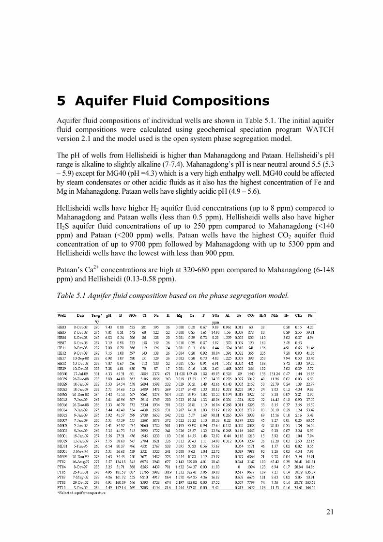
5 Aquifer Fluid Compositions Aquifer fluid compositions of individual wells are shown in Table 5.1. The initial aquifer fluid compositions were calculated using geochemical speciation program WATCH version 2.1 and the model used is the open system phase segregation model.
The pH of wells from Hellisheidi is higher than Mahanagdong and Pataan. Hellisheidi’s pH range is alkaline to slightly alkaline (7-7.4). Mahanagdong’s pH is near neutral around 5.5 (5.3 – 5.9) except for MG40 (pH =4.3) which is a very high enthalpy well. MG40 could be affected by steam condensates or other acidic fluids as it also has the highest concentration of Fe and Mg in Mahanagdong. Pataan wells have slightly acidic pH (4.9 – 5.6).
Hellisheidi wells have higher H2 aquifer fluid concentrations (up to 8 ppm) compared to Mahanagdong and Pataan wells (less than 0.5 ppm). Hellisheidi wells also have higher H2S aquifer fluid concentrations of up to 250 ppm compared to Mahanagdong (<140 ppm) and Pataan (<200 ppm) wells. Pataan wells have the highest CO2 aquifer fluid concentration of up to 9700 ppm followed by Mahanagdong with up to 5300 ppm and Hellisheidi wells have the lowest with less than 900 ppm.
Pataan’s Ca2+ concentrations are high at 320-680 ppm compared to Mahanagdong (6-148 ppm) and Hellisheidi (0.13-0.58 ppm).
Table 5.1 Aquifer fluid composition based on the phase segregation model.
22
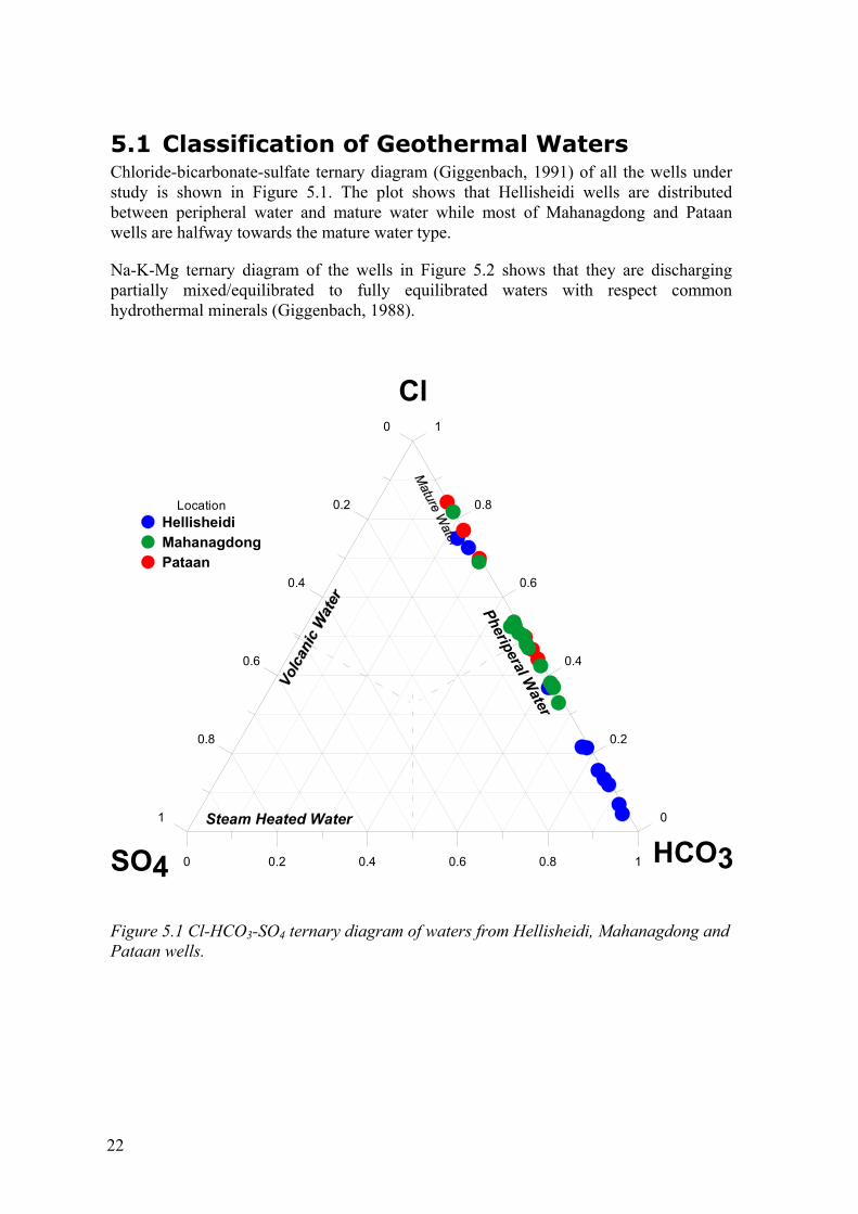
5.1 Classification of Geothermal Waters Chloride-bicarbonate-sulfate ternary diagram (Giggenbach, 1991) of all the wells under study is shown in Figure 5.1. The plot shows that Hellisheidi wells are distributed between peripheral water and mature water while most of Mahanagdong and Pataan wells are halfway towards the mature water type.
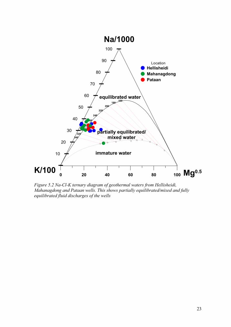
Na-K-Mg ternary diagram of the wells in Figure 5.2 shows that they are discharging partially mixed/equilibrated to fully equilibrated waters with respect common hydrothermal minerals (Giggenbach, 1988).
Cl
SO4 HCO3Steam Heated Water
Pheriperal Water
0 0.2 0.4 0.6 0.8 1
1
0.8
0.6
0.4
0.2
01
0.8
0.6
0.4
0.2
0
LocationHellisheidiMahanagdongPataan
Figure 5.1 Cl-HCO3-SO4 ternary diagram of waters from Hellisheidi, Mahanagdong and Pataan wells.
23
0 20 40 60 80 100
160180
200
220
240
260
280
300320
340
10
20
30
40
50
60
70
80
90
100
LocationHellisheidiMahanagdongPataan
equilibrated water
partially equilibrated/mixed water
immature water
Na/1000
K/100 Mg0.5
Figure 5.2 Na-Cl-K ternary diagram of geothermal waters from Hellisheidi, Mahanagdong and Pataan wells. This shows partially equilibrated/mixed and fully equilibrated fluid discharges of the wells

24
25
6 Results and Discussions
6.1 Mineral Saturation
Saturation index (SI) is used to assess the departure of mineral saturation from the equilibrium and is expressed as
KQSI log=
where Q is the reaction qoutient/activity product of mineral dissolution reaction and K is the equilibrium constant.
Logarithm of activity product/reaction qoutient, log Q, are calculated based from the species activities calculated using WATCH speciation program except for anhydrite mineral saturation which are directly taken from WATCH logQ and logK WATCH output. WATCH uses the thermodynamic data provided by (Arnórsson et al., 1982). Gas solubility constants were taken from Fernandez-Prini (2003). Activities of H4SiO4
o were based from the work of Gunnarsson and Arnórsson (2000).
The standard thermodynamic properties of minerals were selected from the data set of Holland and Powell (1998) except those of pyrite and pyrrhotite which was taken from Robbie and Hemmingway (1995). Dissociation equilibriums for Al-hydroxide species were based from Arnórsson and Andrésdóttir (1999), while ferric- and ferrous hydroxide equilibriums were taken from the work of Diakonov and Tagirov (2002). The Al-Si dimer of Pokrovski et al. (1998) was incorporated into the speciation calculations (Angcoy, 2010).
Table 6.1 lists the mineral dissolution reactions and the associated equilibrium constants taken from Angcoy (2010).
6.1.1 Calcite and Anhydrite
Calcite saturation versus the selected aquifer temperature is shown in Figure 6.1.
At Hellisheidi the aquifer fluids are very close at equilibrium with calcite and when all uncertainties were considered such as analytical imprecision and selection of aquifer temperatures (e.g Angcoy (2010) and Arnorsson (2007)), departure from saturation is not significant. The average departure from calcite saturation of Hellisheidi wells is only 0.05 SI units.
Mahanagdong aquifer fluids are very close to being at equilibrium with respect to calcite. Only MG40 well showed high level of undersaturation of 2.1 SI units. MG40 has high
26
“excess” enthalpy and is acidic which might be affected by injected steam condensates or other acidic fluids. The average calcite saturation of Mahanagdong wells is -0.2 SI units.
Pataan wells fluids were practically at equilibrium with calcite or slightly over-saturated with an average value of 0.2 SI units. Well PT02 is the most oversaturated with 0.74 SI units.
Figure 6.2 shows calcite saturation versus total discharge enthalpy. There was no significant correlation between calcite saturation and discharge enthalpy. MG40 well is not shown. As already mentioned, the aquifer of this well is highly undersaturated.
The calculated saturation index for calcite increases with increasing value of the calculated aquifer pH (Figure 6.3). This is considered to be due to error in the calculated aquifer water pH. Many factors affect the calculated pH, including both analytical data on sample pH, total carbonate carbon and total sulfide sulfur, thermodynamic data on various dissociational equilibria, selected aquifer temperature and the model used to calculate aquifer fluid compositions from wellhead data. It is not possible to identify the main sources of their apparent variation in pH and calcite saturation index but it seems to be significant, particularly in the case of Hellisheidi.
Mahanagdong and Pataan aquifer fluids approach anhydrite equilibrium as shown in Figure 6.4 whereas Hellisheidi waters are considerably anhydrite undersaturated.
6.1.2 Magnetie, Pyrite and Pyrrhotite
Figure 6.5 shows the equilibrium curve for the redox reactions involving pyrite, magnetite, H2S and H2. At equilibrium this reaction gives the aqueous H2S and H2 molal ratios. Hellisheidi aquifer waters are quite close to equilibrium, with an average of 0.03 log units above the curve. Mahanagdong and Pataan aquifer waters are systematically with higher H2S/H2 ratios than those corresponding to equilibrium, by 0.2 and 0.55 log units on average, respectively.
Figure 6.6 shows the equilibrium curve for the redox reactions involving pyrite, pyrrhotite, H2S and H2. Hellisheidi aquifer waters are very close to equilibrium yet systematically below the equilibrium curve on average by 0.25 log units, if the degassed discharge of HE03and HE05 are excluded. Mahanagdong and Pataan aquifer waters are systematically with higher H2S/H2 ratios than those corresponding to equilibrium, by 0.96 and 1.3 log units on average, respectively. Clearly the H2S/H2 ratios in the aquifer waters in the Philippine geothermal fields are not controlled by pyrite-pyrrhotite buffer.
27
250 260 270 280 290 300 310Aquifer Temperature, oC
-2
-1
0
1
2
-2
-1
0
1
2
Cal
cite
Sat
urat
ion
Inde
x, lo
g (Q
/K)
-2
-1
0
1
2
CaCO3 + 2H+ = Ca2+ + CO2(aq) + H2O(l)
Hellisheidi
Mahanagdong
Pataan
MG40
Figure 6.1 Calcite saturation index of aquifer fluid versus the selected aquifer temperature.
28
800 1200 1600 2000 2400 2800Total Discharge Enthalpy, kJ/kg
-2
-1
0
1
2
-2
-1
0
1
2
Cal
cite
Sat
urat
ion
Inde
x, lo
g (Q
/K)
-2
-1
0
1
2
LocationHellisheidiMahanagdongPataan
CaCO3 + 2H+ = Ca2+ + CO2(aq) + H2O(l)
Figure 6.2 Calcite saturation index of aquifer fluid versus total discharge enthalpies.
29
4.5 5 5.5 6 6.5 7 7.5Aquifer pH
-2
0
2
-2
-1
0
1
2
Cal
cite
Sat
urat
ion
Inde
x, lo
g (Q
/K)
-2
-1
0
1
2
LocationHellisheidiMahanagdongPataan
CaCO3 + 2H+ = Ca2+ + CO2(aq) + H2O(l)
Figure 6.3 Calcite saturation index versus pH of the aquifer fluid.
30
Table 6.1 Log K-temperature equations of individual mineral dissolution reactions (valid at 0-350°C at Psat, unit activity for all minerals and liquid water) modified after Angcoy (2010).
cal-calcite, czo-clinozoisite, epi-epidote, gro-grossular, mag-magnetite, pre-prehnite, pyr-pyrite, pyrr-pyrrhotite, qtz-quartz, wol-wollastonite
31
250 260 270 280 290 300 310Aquifer Temperature, oC
-3
-2
-1
0
1
2
3-3
-2
-1
0
1
2
3
Anh
ydrit
e Sa
tura
tion
Inde
x, lo
g (Q
/K)
-3
-2
-1
0
1
2
3
CaSO4 = Ca2+ + SO42-
Hellisheidi
Mahanagdong
Pataan
Figure 6.4 Anhydrite saturation index of aquifer fluid versus the selected aquifer temperature.
32
240 260 280 300 320Aquifer Temperature, oC
-3
-2
-1
0
log
(H2S
) - /
3 1
log
(H2)
PataanMahanagdongHellisheidi
/31 H2,aq + /21 pyr + /32 H2O = /61 mag + H2Saq
HE03
HE29
Figure 6.5 Aquifer fluid H2S and H2 molal ratios in relation to the equilibrium curve of pyrite-magnetite mineral assemblage.
200 250 300 350Aquifer Temperature, oC
-1
0
1
2
3
log
(H2S
) - lo
g (H
2)
Geothermal FieldsPataanMahanagdongHellisheidi
H2,aq + pyr = pyrr + H2Saq
HE03
HE05
Figure 6.6 Aquifer fluid H2S and H2 molal ratios in relation to the equilibrium curve of pyrite-pyyrhotite mineral assemblage.
33
6.2 Effect of Boiling and Degassing
Mineral deposition from the boiling fluid largely occurs in response to its cooling and degassing. Cooling causes geothermal waters to become over-saturated with minerals with prograde solubility but under-saturated with those having retrograde solubility. Degassing tends to produce over-saturated water with respect to minerals whose solubility decreases with increasing pH. The quantity of minerals precipitated from solution is not only determined by the degree of over-saturation but also by the fluid composition and the kinetics of the precipitation reaction. The solubility of some minerals decreases with increasing temperature and increasing pH; an example being calcite. The combined effects of both processes, together with the rate of the precipitation reaction, determine whether or not the minerals with which the water becomes over-saturated precipitate from solution. Un-boiled geothermal liquids are typically close to being calcite-saturated as shown from this study and others (Arnórsson, 1989). Extensive degassing by boiling tends to cause an initially calcite-saturated water to become over-saturated. The cooling has the opposite effect due to the retrograde solubility of calcite with respect to temperature. The extent of degassing and cooling determine whether boiling causes an initially calcite saturated water to become over or under-saturated (Arnorsson et al., 2007).
6.2.1 Hellisheidi Wells
Figures 6.7 to 6.15 show how the degree of calcite saturation varies during adiabatic boiling at different extent of degassing for all analyzed gases (CO2, H2S, H2, CH4, N2) in Hellishedi wells. The dots show the calculated calcite saturation in the aquifer for each well. An overall pattern in the variation of the saturation index (SI) of Hellisheidi wells with temperature is observed from all the wells except well HE03. The SI initially increases then, after it reaches a peak, decreases to negative values. The initial increase in SI reflects an increase in pH due to CO2 and H2S degassing. The pH increase causes a strong increase in the activity of the CO3
−2 species. At maximum SI values, the water has been largely degassed, and the subsequent decline in SI is caused by increased calcite solubility with decreasing temperature (Arnorsson et al., 2007). Well HE03 is an exception to the general trend because the fluid entering the well is highly degassed as reflected by the low gas content of the discharge; therefore, SI decreases immediately during adiabatic boiling.
The extent of degassing (as expressed by the degassing coefficient) increases the level of calcite SI except for degassed well HE03 which shows the opposite. The value of the degassing coefficient can be arbitrarily selected when running the WATCH program. A value of 1 represent maximum degassing, i.e. equilibrium distribution of all gases is attained between liquid and vapor. A degassing coefficient of e.g. 0.5 implies that degassing is taken to be 50% maximum. For degassing to occur during boiling, a mass transfer of gases occurs from the liquid to vapor. In reality such degassing is often incomplete as shown by analysis of CO2 in liquid water and water in steam separators.
34
80 120 160 200 240 280Temperature, oC
-3
-2
-1
0
1C
alci
te S
atur
atio
n, L
og(Q
/K)
HE03Degas. Coeff =1.0Degas. Coeff =0.5Degas. Coeff =0.2
Figure 6.7 Calcite saturation of well HE03 during adiabatic boiling at different degassing coefficients.
80 120 160 200 240 280Temperature, oC
-1
-0.5
0
0.5
1
Cal
cite
Sat
urat
ion,
Log
Q/K HE05
Degas. Coeff =1.0Degas. Coeff =0.5Degas. Coeff =0.2
Figure 6.8 Calcite saturation of well HE05 during adiabatic boiling at different degassing coefficients.
35
80 120 160 200 240 280Temperature, oC
-1
-0.5
0
0.5
1C
alci
te S
atur
atio
n, L
og Q
/K HE06Degas. Coeff =1.0Degas. Coeff =0.5Degas. Coeff =0.2
Figure 6.9 Calcite saturation of well HE06 during adiabatic boiling at different degassing coefficients.
80 120 160 200 240 280Temperature, oC
-1.5
-1
-0.5
0
0.5
Cal
cite
Sat
urat
ion,
Log
Q/K
HE07Degas. Coeff =1.0Degas. Coeff =0.5Degas. Coeff =0.2
Figure 6.10 Calcite saturation of well HE07 during adiabatic boiling at different degassing coefficients.
36
80 120 160 200 240 280 320Temperature, oC
-1.5
-1
-0.5
0
0.5
Cal
cite
Sat
urat
ion
Inde
x, L
og(Q
/K)
HE11Degas. Coeff =1.0Degas. Coeff =0.5Degas. Coeff =0.2
Figure 6.11 Calcite saturation of well HE11 during adiabatic boiling at different degassing coefficients.
80 120 160 200 240 280 320Temperature, oC
-1.5
-1
-0.5
0
0.5
Cal
cite
Sat
urat
ion
Inde
x, L
og Q
/K
HE12Degas. Coeff =1.0Degas. Coeff =0.5Degas. Coeff =0.2
Figure 6.12 Calcite saturation of well HE12 during adiabatic boiling at different degassing coefficients.
37
80 120 160 200 240 280 320Temperature, oC
-2
-1.5
-1
-0.5
0C
alci
te S
atur
atio
n In
dex,
Log
Q/K
HE17Degas. Coeff =1.0Degas. Coeff =0.5Degas. Coeff =0.2
Figure 6.13 Calcite saturation of well HE17 during adiabatic boiling at different degassing coefficients.
80 120 160 200 240 280Temperature, oC
-1.5
-1
-0.5
0
0.5
Cal
cite
Sat
urat
ion
Inde
x, L
og Q
/K
HE18Degas. Coeff =1.0Degas. Coeff =0.5Degas. Coeff =0.2
Figure 6.14 Calcite saturation of well HE18 during adiabatic boiling at different degassing coefficients.
6.2.2 Mahanagdong Wells
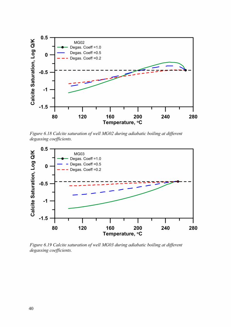
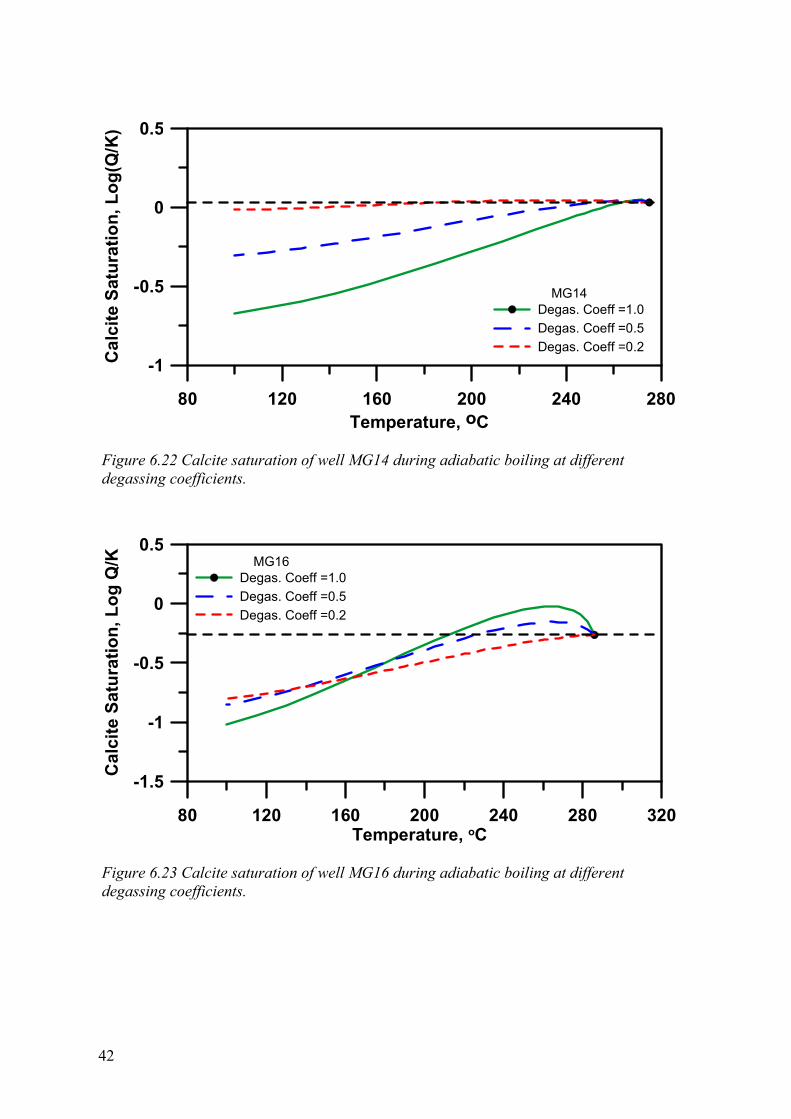
The majority of the wells in Mahanagdong follow the general pattern exhibited by Hellisheidi wells (Figures 6.16 to 6.31). Exception includes MG40, MG29, MG14 and MG03. MG40 is a high “excess” enthalpy and acidic well. MG03 and MG14 are postulated to be receiving fluid from the upflow zone but have been affected by brine injection returns. The reservoir chloride
38
levels of MG03 and MG14 are shifted towards the composition of the injected brine. The total discharge CO2 concentrations of MG03 declined and the total discharge enthalpy of MG14 declined. Well MG29, on the other hand, is located in the western periphery of the Mahanagdong geothermal system and could be affected by intrusion of cooler peripheral waters(Figure 6.32, Salonga et al., 2004).
100 150 200 250 300 350Temperature, oC
-2
-1.5
-1
-0.5
0
0.5
Cal
cite
Sat
urat
ion
Inde
x, L
og Q
/K
HE29Degas. Coeff =1.0Degas. Coeff =0.5Degas. Coeff =0.2
Figure 6.15 Calcite saturation of well HE29 during adiabatic boiling at different degassing coefficients.
The highest positive departure from the initial saturation in Mahanagdong is from MG19, with 0.40 (at 251 oC) SI units above the initial saturation at its most degassed state (degassing coefficient of 1.0). MG19 is known to deposit calcite scale in the well.
Figure 6.17 shows the calcite saturation of MG01 prior to production (1994 water and gas analyses). Boiling of the aquifer fluid of this well produces the highest increase in calcite over-saturation of 0.51 SI units. Comparing MG01 CO2 and H2S aquifer fluid concentrations on samples taken in 2009 and 1994 shows that it has been partially degassed or mixed with degassed injected brine. Aquifer fluid CO2 concentration decreased from 8000 to 1200 ppm and H2S concentration decreased from 92 to 15 ppm. Activity of free Ca2+ probably affects the calcite saturation because it partially increased (from 10 to 16 ppm) in 1994 to 2009 samples.
The case of MG19 is similar with MG01. The present fluid discharge is partially degassed or mixed with injected brine and Ca2+ concentration has increased. Aquifer fluid CO2 concentration decreased from 6900 to 3200 ppm, H2S concentration decreased from 71 to 36 ppm and Ca2+ increased from 11 to 20 ppm. Calcite mineral SI trend of MG19 practically remains the same after almost 15 years of production though the old data shows a higher departure of 0.48 SI units above the initial saturation, Figures 6.25 and 6.26.
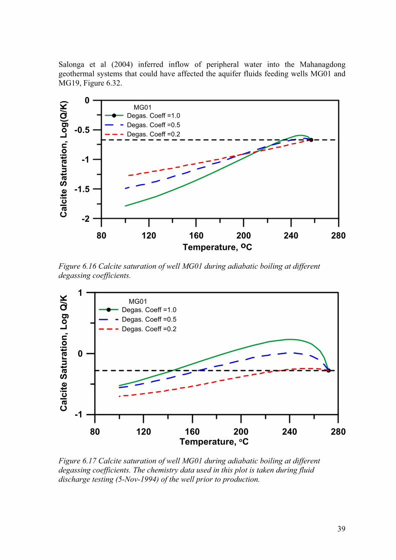
39
Salonga et al (2004) inferred inflow of peripheral water into the Mahanagdong geothermal systems that could have affected the aquifer fluids feeding wells MG01 and MG19, Figure 6.32.
80 120 160 200 240 280Temperature, oC
-2
-1.5
-1
-0.5
0
Cal
cite
Sat
urat
ion,
Log
(Q/K
)
MG01Degas. Coeff =1.0Degas. Coeff =0.5Degas. Coeff =0.2
Figure 6.16 Calcite saturation of well MG01 during adiabatic boiling at different degassing coefficients.
80 120 160 200 240 280Temperature, oC
-1
0
1
Cal
cite
Sat
urat
ion,
Log
Q/K MG01
Degas. Coeff =1.0Degas. Coeff =0.5Degas. Coeff =0.2
Figure 6.17 Calcite saturation of well MG01 during adiabatic boiling at different degassing coefficients. The chemistry data used in this plot is taken during fluid discharge testing (5-Nov-1994) of the well prior to production.
40
80 120 160 200 240 280Temperature, oC
-1.5
-1
-0.5
0
0.5C
alci
te S
atur
atio
n, L
og Q
/K MG02Degas. Coeff =1.0Degas. Coeff =0.5Degas. Coeff =0.2
Figure 6.18 Calcite saturation of well MG02 during adiabatic boiling at different degassing coefficients.
80 120 160 200 240 280Temperature, oC
-1.5
-1
-0.5
0
0.5
Cal
cite
Sat
urat
ion,
Log
Q/K MG03
Degas. Coeff =1.0Degas. Coeff =0.5Degas. Coeff =0.2
Figure 6.19 Calcite saturation of well MG03 during adiabatic boiling at different degassing coefficients.
41
80 120 160 200 240 280Temperature, oC
-1.5
-1
-0.5
0
0.5C
alci
te S
atur
atio
n, L
og Q
/K
MG07Degas. Coeff =1.0Degas. Coeff =0.5Degas. Coeff =0.2
Figure 6.20 Calcite saturation of well MG07 during adiabatic boiling at different degassing coefficients.
80 120 160 200 240 280 320Temperature, oC
-1.5
-1
-0.5
0
0.5
Cal
cite
Sat
urat
ion,
Log
Q/K
MG13Degas. Coeff =1.0Degas. Coeff =0.5Degas. Coeff =0.2
Figure 6.21 Calcite saturation of well MG13 during adiabatic boiling at different degassing coefficients.
42
80 120 160 200 240 280Temperature, oC
-1
-0.5
0
0.5C
alci
te S
atur
atio
n, L
og(Q
/K)
MG14Degas. Coeff =1.0Degas. Coeff =0.5Degas. Coeff =0.2
Figure 6.22 Calcite saturation of well MG14 during adiabatic boiling at different degassing coefficients.
80 120 160 200 240 280 320Temperature, oC
-1.5
-1
-0.5
0
0.5
Cal
cite
Sat
urat
ion,
Log
Q/K MG16
Degas. Coeff =1.0Degas. Coeff =0.5Degas. Coeff =0.2
Figure 6.23 Calcite saturation of well MG16 during adiabatic boiling at different degassing coefficients.
43
80 120 160 200 240 280Temperature, oC
-1.5
-1
-0.5
0
0.5C
alci
te S
atur
atio
n, L
og Q
/K MG18Degas. Coeff =1.0Degas. Coeff =0.5Degas. Coeff =0.2
Figure 6.24 Calcite saturation of well MG18 during adiabatic boiling at different degassing coefficients.
80 120 160 200 240 280Temperature, oC
-1
-0.5
0
0.5
1
Cal
cite
Sat
urat
ion,
Log
Q/K MG19
Degas. Coeff =1.0Degas. Coeff =0.5Degas. Coeff =0.2
Figure 6.25 Calcite saturation of well MG19 during adiabatic boiling at different degassing coeffients.
44
80 120 160 200 240 280Temperature, oC
-1
-0.5
0
0.5
1C
alci
te S
atur
atio
n, L
og Q
/K MG19Degas. Coeff =1.0Degas. Coeff =0.5Degas. Coeff =0.2
Figure 6.26 Calcite saturation of well MG19 during adiabatic boiling at different degassing coefficients. The chemistry data used in this plot is taken during fluid discharge testing (20-Dec-1995) of the well prior to production.
80 120 160 200 240 280 320Temperature, oC
-1
-0.5
0
0.5
Cal
cite
Sat
urat
ion,
Log
Q/K MG22
Degas. Coeff =1.0Degas. Coeff =0.5Degas. Coeff =0.2
Figure 6.27 Calcite saturation of well MG22 during adiabatic boiling at different degassing coefficients.
45
80 120 160 200 240 280Temperature, oC
-1
-0.75
-0.5
-0.25
0
0.25
0.5C
alci
te S
atur
atio
n, L
og(Q
/K)
MG23Degas. Coeff =1.0Degas. Coeff =0.5Degas. Coeff =0.2
Figure 6.28 Calcite saturation of well MG23 during adiabatic boiling at different degassing coefficients.
80 120 160 200 240 280 320Temperature, oC
-1.5
-1
-0.5
0
0.5
Cal
cite
Sat
urat
ion,
Log
Q/K
MG29Degas. Coeff =1.0Degas. Coeff =0.5Degas. Coeff =0.2
Figure 6.29 Calcite saturation of well MG29 during adiabatic boiling at different degassing coefficients.
46
80 120 160 200 240 280 320Temperature, oC
MG39Degas. Coeff =1.0Degas. Coeff =0.5Degas. Coeff =0.2
-1
-0.5
0
0.5
1C
alci
te S
atur
atio
n, L
og Q
/K
Figure 6.30 Calcite saturation of well MG39 during adiabatic boiling at different degassing coefficients.
100 150 200 250 300 350Temperature, oC
-3
-2
-1
0
Cal
cite
Sat
urat
ion,
Log
Q/K MG40
Degas. Coeff =1.0Degas. Coeff =0.5Degas. Coeff =0.2
Figure 6.31 Calcite saturation of well MG40 during adiabatic boiling at different degassing coefficients.

47
Figure 6.32 Inferred fluid flow paths at Mahanagdong geothermal field. Based on Salonga et al ( 2004).
6.2.3 Pataan Wells
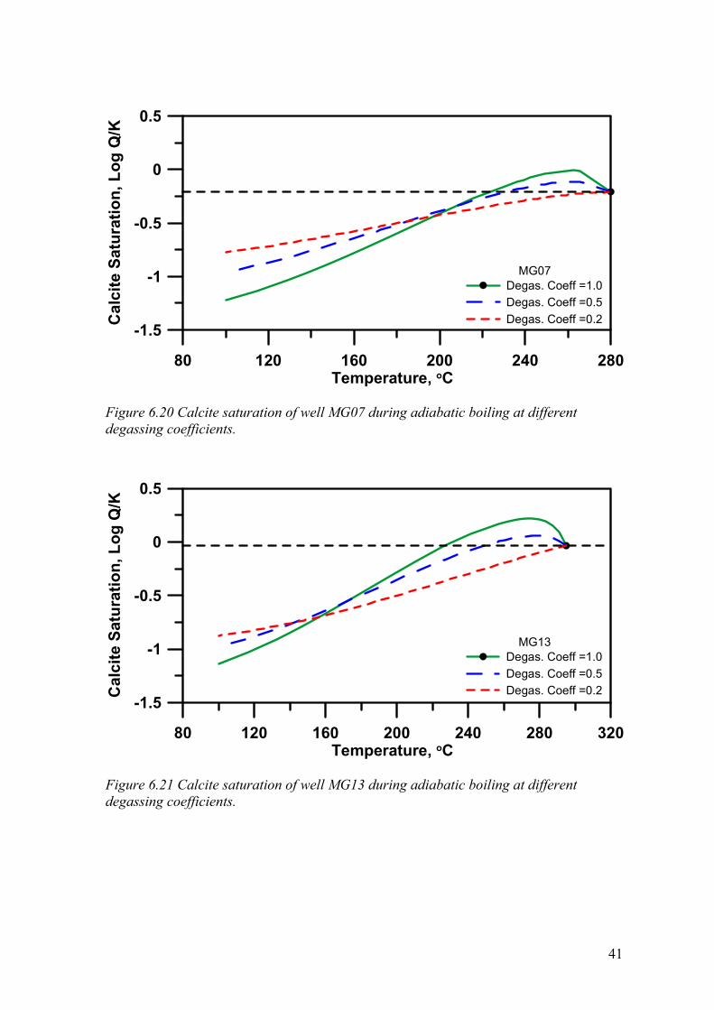
Pataan aquifer fluids show trends similar to those of Hellisheidi and most of the Mahanagdong wells (Figures 6.33 to 6.38). During boiling the calcite saturation increases initially followed by a decline. The extent of degassing (increase in degassing coefficient) increases the degree of oversaturation. Well PT08 has the highest departure of 0.6 SI units (at 223 oC) above the initial saturation followed by PT05, PT10 and PT07 with 0.40 (at 246 oC), 0.31(at 258 oC) and 0.28 (at 252 oC) SI units above the the initial
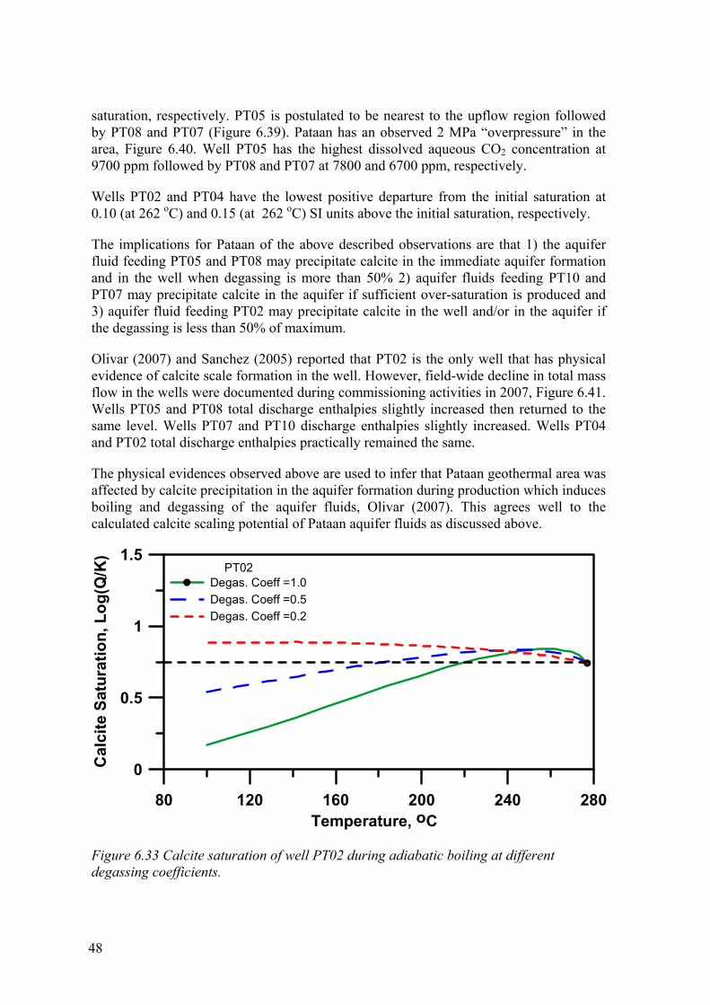
48
saturation, respectively. PT05 is postulated to be nearest to the upflow region followed by PT08 and PT07 (Figure 6.39). Pataan has an observed 2 MPa “overpressure” in the area, Figure 6.40. Well PT05 has the highest dissolved aqueous CO2 concentration at 9700 ppm followed by PT08 and PT07 at 7800 and 6700 ppm, respectively.
Wells PT02 and PT04 have the lowest positive departure from the initial saturation at 0.10 (at 262 oC) and 0.15 (at 262 oC) SI units above the initial saturation, respectively.
The implications for Pataan of the above described observations are that 1) the aquifer fluid feeding PT05 and PT08 may precipitate calcite in the immediate aquifer formation and in the well when degassing is more than 50% 2) aquifer fluids feeding PT10 and PT07 may precipitate calcite in the aquifer if sufficient over-saturation is produced and 3) aquifer fluid feeding PT02 may precipitate calcite in the well and/or in the aquifer if the degassing is less than 50% of maximum.
Olivar (2007) and Sanchez (2005) reported that PT02 is the only well that has physical evidence of calcite scale formation in the well. However, field-wide decline in total mass flow in the wells were documented during commissioning activities in 2007, Figure 6.41. Wells PT05 and PT08 total discharge enthalpies slightly increased then returned to the same level. Wells PT07 and PT10 discharge enthalpies slightly increased. Wells PT04 and PT02 total discharge enthalpies practically remained the same.
The physical evidences observed above are used to infer that Pataan geothermal area was affected by calcite precipitation in the aquifer formation during production which induces boiling and degassing of the aquifer fluids, Olivar (2007). This agrees well to the calculated calcite scaling potential of Pataan aquifer fluids as discussed above.
80 120 160 200 240 280Temperature, oC
0
0.5
1
1.5
Cal
cite
Sat
urat
ion,
Log
(Q/K
)
PT02Degas. Coeff =1.0Degas. Coeff =0.5Degas. Coeff =0.2
Figure 6.33 Calcite saturation of well PT02 during adiabatic boiling at different degassing coefficients.
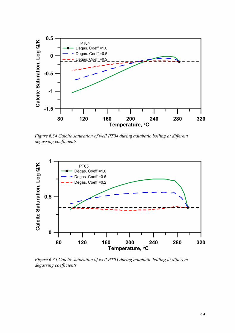
49
80 120 160 200 240 280 320Temperature, oC
-1.5
-1
-0.5
0
0.5C
alci
te S
atur
atio
n, L
og Q
/K PT04Degas. Coeff =1.0Degas. Coeff =0.5Degas. Coeff =0.2
Figure 6.34 Calcite saturation of well PT04 during adiabatic boiling at different degassing coefficients.
80 120 160 200 240 280 320Temperature, oC
0
0.5
1
Cal
cite
Sat
urat
ion,
Log
Q/K PT05
Degas. Coeff =1.0Degas. Coeff =0.5Degas. Coeff =0.2
Figure 6.35 Calcite saturation of well PT05 during adiabatic boiling at different degassing coefficients.
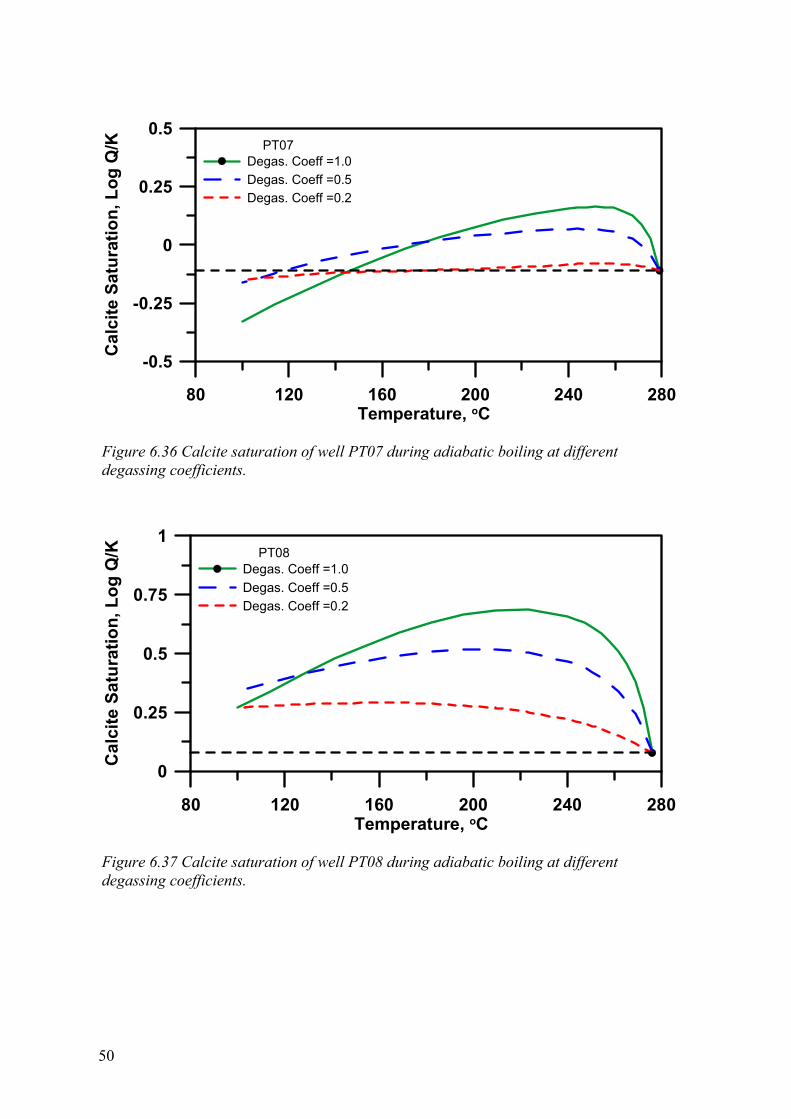
50
80 120 160 200 240 280Temperature, oC
-0.5
-0.25
0
0.25
0.5C
alci
te S
atur
atio
n, L
og Q
/K PT07Degas. Coeff =1.0Degas. Coeff =0.5Degas. Coeff =0.2
Figure 6.36 Calcite saturation of well PT07 during adiabatic boiling at different degassing coefficients.
80 120 160 200 240 280Temperature, oC
0
0.25
0.5
0.75
1
Cal
cite
Sat
urat
ion,
Log
Q/K PT08
Degas. Coeff =1.0Degas. Coeff =0.5Degas. Coeff =0.2
Figure 6.37 Calcite saturation of well PT08 during adiabatic boiling at different degassing coefficients.
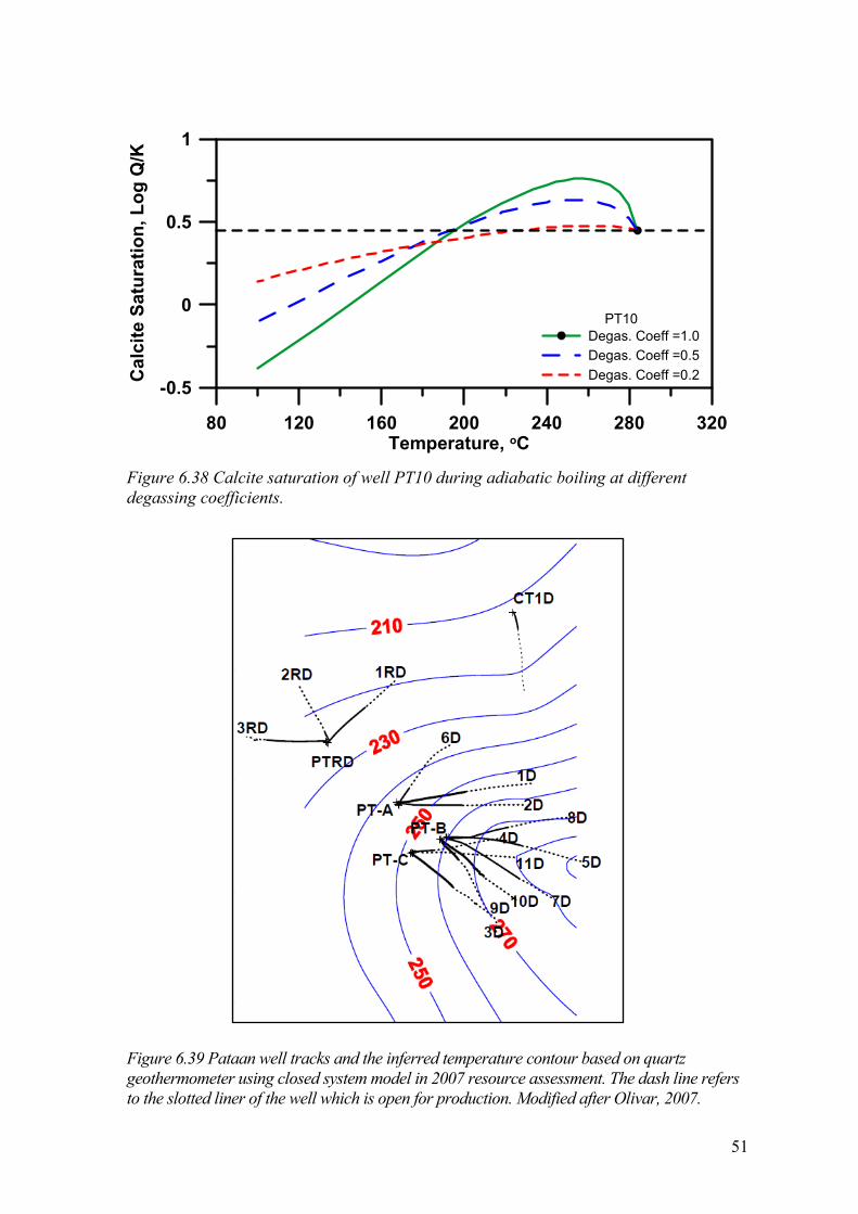
51
80 120 160 200 240 280 320Temperature, oC
-0.5
0
0.5
1C
alci
te S
atur
atio
n, L
og Q
/K
PT10Degas. Coeff =1.0Degas. Coeff =0.5Degas. Coeff =0.2
Figure 6.38 Calcite saturation of well PT10 during adiabatic boiling at different degassing coefficients.
Figure 6.39 Pataan well tracks and the inferred temperature contour based on quartz geothermometer using closed system model in 2007 resource assessment. The dash line refers to the slotted liner of the well which is open for production. Modified after Olivar, 2007.
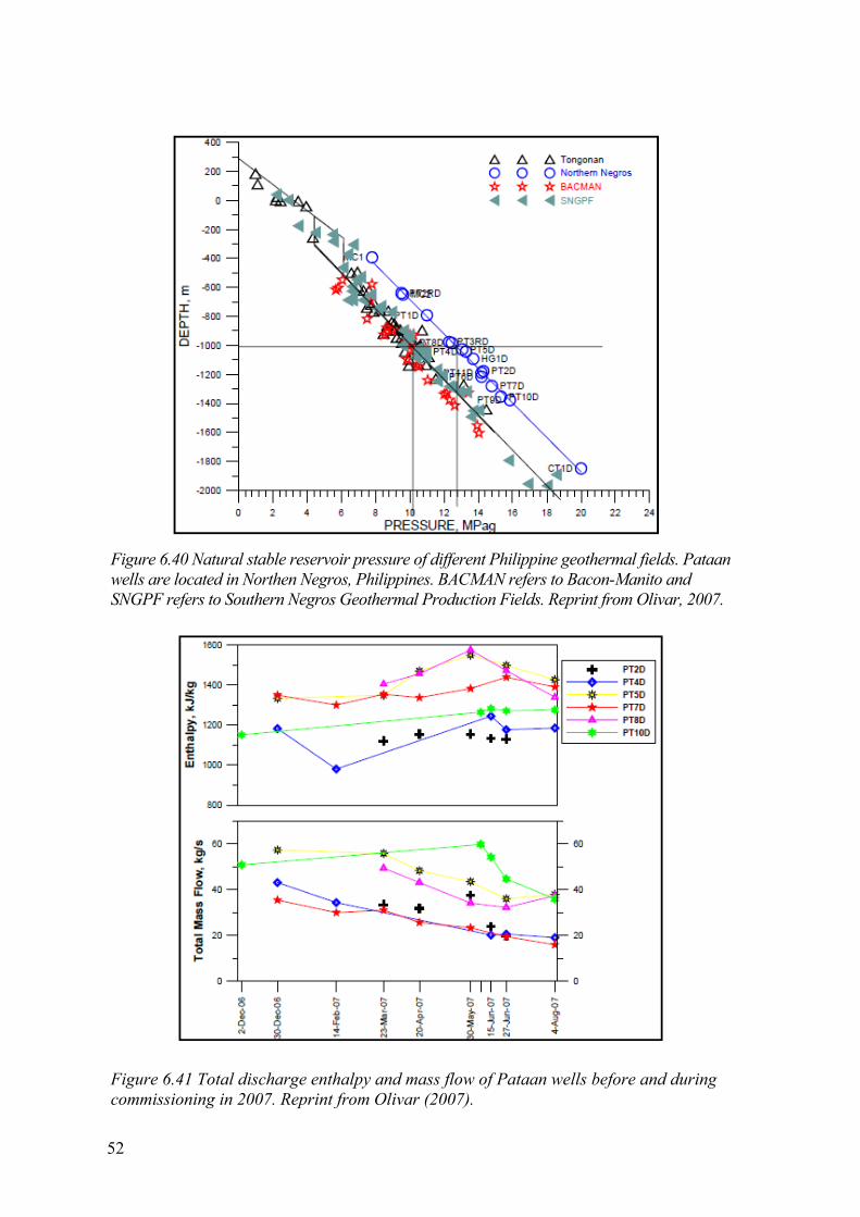
52
Figure 6.40 Natural stable reservoir pressure of different Philippine geothermal fields. Pataan wells are located in Northen Negros, Philippines. BACMAN refers to Bacon-Manito and SNGPF refers to Southern Negros Geothermal Production Fields. Reprint from Olivar, 2007.
Figure 6.41 Total discharge enthalpy and mass flow of Pataan wells before and during commissioning in 2007. Reprint from Olivar (2007).
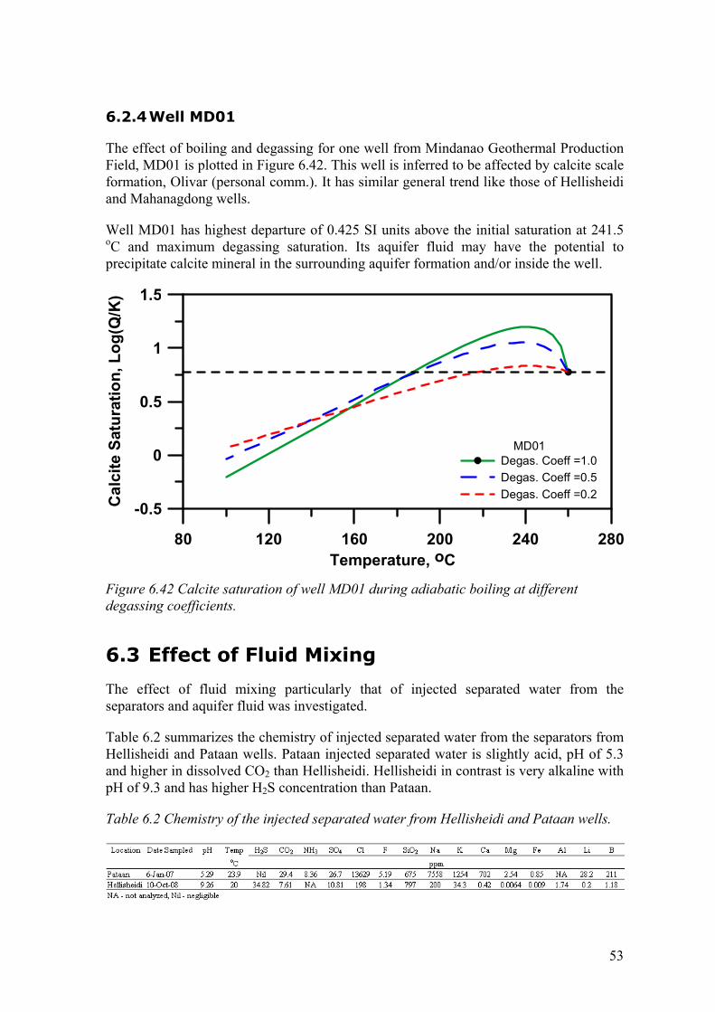
53
6.2.4 Well MD01
The effect of boiling and degassing for one well from Mindanao Geothermal Production Field, MD01 is plotted in Figure 6.42. This well is inferred to be affected by calcite scale formation, Olivar (personal comm.). It has similar general trend like those of Hellisheidi and Mahanagdong wells.
Well MD01 has highest departure of 0.425 SI units above the initial saturation at 241.5 oC and maximum degassing saturation. Its aquifer fluid may have the potential to precipitate calcite mineral in the surrounding aquifer formation and/or inside the well.
80 120 160 200 240 280Temperature, oC
-0.5
0
0.5
1
1.5
Cal
cite
Sat
urat
ion,
Log
(Q/K
)
MD01Degas. Coeff =1.0Degas. Coeff =0.5Degas. Coeff =0.2
Figure 6.42 Calcite saturation of well MD01 during adiabatic boiling at different degassing coefficients.
6.3 Effect of Fluid Mixing
The effect of fluid mixing particularly that of injected separated water from the separators and aquifer fluid was investigated.
Table 6.2 summarizes the chemistry of injected separated water from the separators from Hellisheidi and Pataan wells. Pataan injected separated water is slightly acid, pH of 5.3 and higher in dissolved CO2 than Hellisheidi. Hellisheidi in contrast is very alkaline with pH of 9.3 and has higher H2S concentration than Pataan.
Table 6.2 Chemistry of the injected separated water from Hellisheidi and Pataan wells.

54
The composition of the fluid mixtures are simulated using the aqueous modeling code PHREEQC-2 version 2.17.00 from the graphical interface PHREEQC for Windows develop by Vincent Post (http://www.falw.vu/~posv/phreeqc/index.html). PHREEQC is a hydrogeochemical transport model developed by D.L. Parkhurst and C.A.J Appelo (1999). The thermodynamic database used is phreeqc.dat which is slightly modified version of the database used in PHREEQE (Parkhurst et al., 1980). Caution must be taken into account in the interpretation of the results, however, since PHREEQC is mostly used for low-temperature aqueous geochemical speciation. An example of PHREEQC input file used in the simulation is included in Appendix A.
The mixed fluid was inputted into WATCH 2.1 to simulate boiling and degassing. Table 6.3 and 6.4 show the compositions of the mixed fluids of Hellisheidi and Pataan wells, respectively at different proportions of injected separated water. Pataan separated water from the separators is being injected at temperature of 160 oC, which is used in the simulations of both Hellisheidi and Pataan fluid mixing.
Calcite saturation indices of Hellisheidi mixed fluids are shown in Figures 6.43 to 6.51. Calcite saturation indices of the mixed fluids dropped to below the original saturation of aquifer fluids. Increasing the injected separated water proportion in the mixture decreases the calcite saturation index of the mixed fluid. Saturation indices of the mixed fluids upon boiling are below that of the initial aquifer fluids except at well HE11 where at 30% mix injected separated water, the saturation approach that of the initial aquifer fluid saturation.
80 120 160 200 240 280Temperature, oC
-4
-3
-2
-1
0
1
Cal
cite
Sat
urat
ion,
Log
(Q/K
)
HE03Aquifer fluid5% injected separated water10% injected separated water30% injected separated water
Figure 6.43 Calcite saturation of mixed fluids of well HE03 during adiabatic boiling at equilibrium degassing.
Plots of calcite mineral saturations of Pataan wells are shown in Figures 6.52 to 6.57. Calcite mineral saturation of the mixed fluids also dropped to below the original aquifer fluid saturation at low mixing proportions (5 and 10% injected separated water mixtures). However, increasing the injected separated water proportion in the mixture increases the calcite saturation index of the fluid mixtures. It seems that mixing injected separated
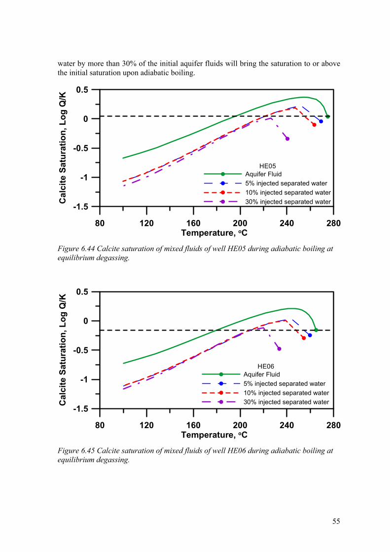
55
water by more than 30% of the initial aquifer fluids will bring the saturation to or above the initial saturation upon adiabatic boiling.
80 120 160 200 240 280Temperature, oC
-1.5
-1
-0.5
0
0.5
Cal
cite
Sat
urat
ion,
Log
Q/K
HE05Aquifer Fluid5% injected separated water10% injected separated water30% injected separated water
Figure 6.44 Calcite saturation of mixed fluids of well HE05 during adiabatic boiling at equilibrium degassing.
80 120 160 200 240 280Temperature, oC
-1.5
-1
-0.5
0
0.5
Cal
cite
Sat
urat
ion,
Log
Q/K
HE06Aquifer Fluid5% injected separated water10% injected separated water30% injected separated water
Figure 6.45 Calcite saturation of mixed fluids of well HE06 during adiabatic boiling at equilibrium degassing.
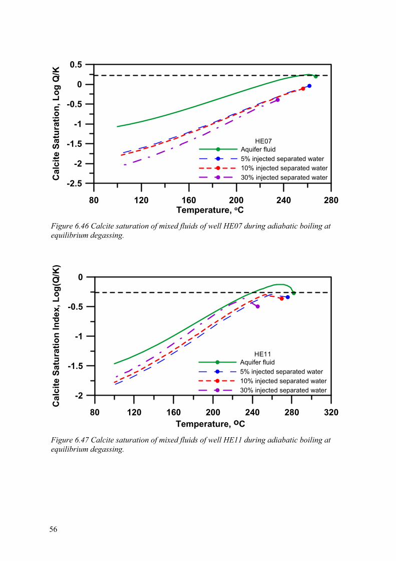
56
80 120 160 200 240 280Temperature, oC
-2.5
-2
-1.5
-1
-0.5
0
0.5C
alci
te S
atur
atio
n, L
og Q
/K
HE07Aquifer fluid5% injected separated water10% injected separated water30% injected separated water
Figure 6.46 Calcite saturation of mixed fluids of well HE07 during adiabatic boiling at equilibrium degassing.
80 120 160 200 240 280 320Temperature, oC
-2
-1.5
-1
-0.5
0
Cal
cite
Sat
urat
ion
Inde
x, L
og(Q
/K)
HE11Aquifer fluid5% injected separated water10% injected separated water30% injected separated water
Figure 6.47 Calcite saturation of mixed fluids of well HE11 during adiabatic boiling at equilibrium degassing.
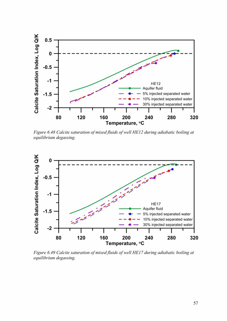
57
80 120 160 200 240 280 320Temperature, oC
-2
-1.5
-1
-0.5
0
0.5C
alci
te S
atur
atio
n In
dex,
Log
Q/K
HE12Aquifer fluid5% injected separated water10% injected separated water30% injected separated water
Figure 6.48 Calcite saturation of mixed fluids of well HE12 during adiabatic boiling at equilibrium degassing.
80 120 160 200 240 280 320Temperature, oC
-2
-1.5
-1
-0.5
0
Cal
cite
Sat
urat
ion
Inde
x, L
og Q
/K
HE17Aquifer fluid5% injected separated water10% injected separated water30% injected separated water
Figure 6.49 Calcite saturation of mixed fluids of well HE17 during adiabatic boiling at equilibrium degassing.
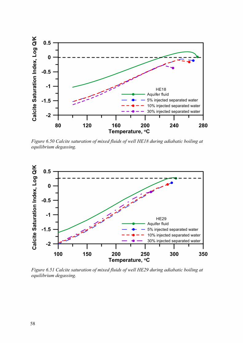
58
80 120 160 200 240 280Temperature, oC
-2
-1.5
-1
-0.5
0
0.5C
alci
te S
atur
atio
n In
dex,
Log
Q/K
HE18Aquifer fluid5% injected separated water10% injected separated water30% injected separated water
Figure 6.50 Calcite saturation of mixed fluids of well HE18 during adiabatic boiling at equilibrium degassing.
100 150 200 250 300 350Temperature, oC
-2
-1.5
-1
-0.5
0
0.5
Cal
cite
Sat
urat
ion
Inde
x, L
og Q
/K
HE29Aquifer fluid5% injected separated water10% injected separated water30% injected separated water
Figure 6.51 Calcite saturation of mixed fluids of well HE29 during adiabatic boiling at equilibrium degassing.
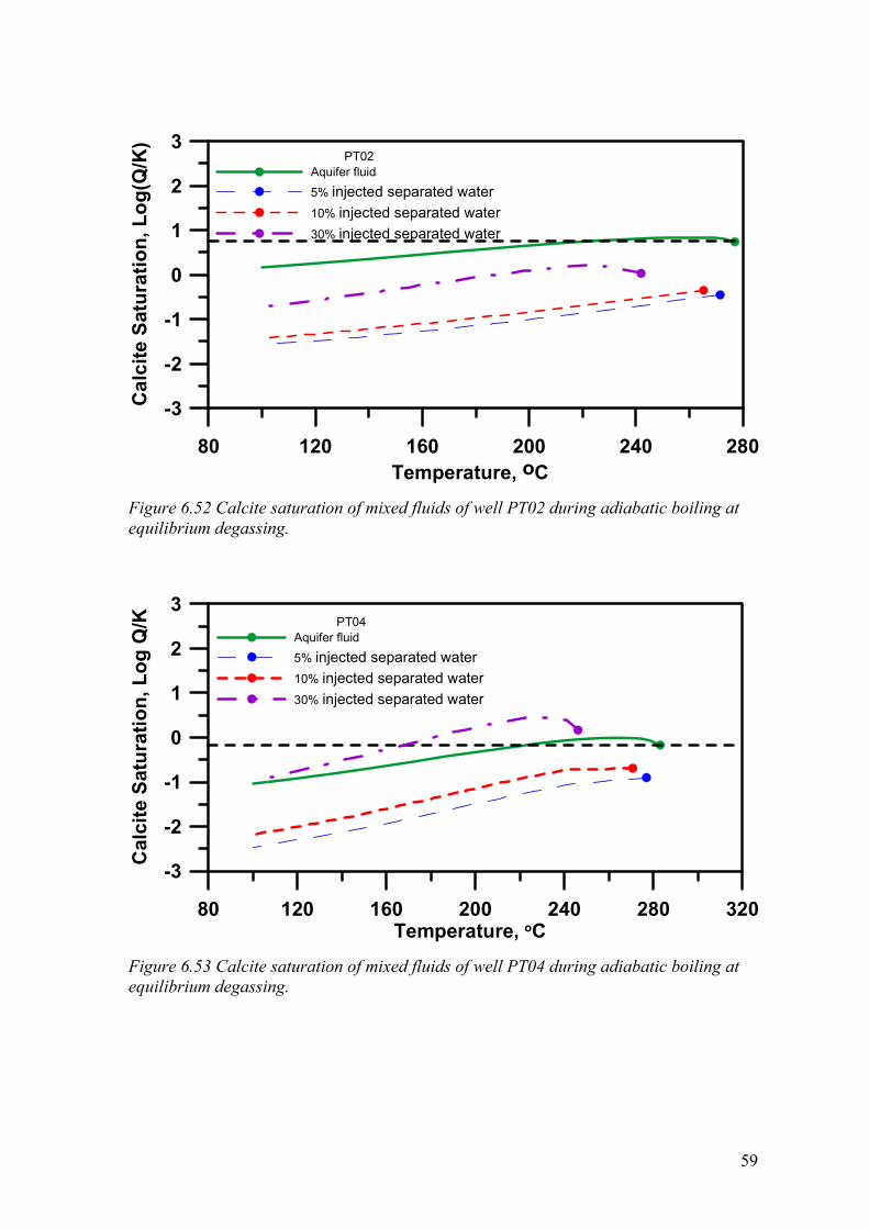
59
80 120 160 200 240 280Temperature, oC
-3
-2
-1
0
1
2
3C
alci
te S
atur
atio
n, L
og(Q
/K)
PT02Aquifer fluid
5% injected separated water10% injected separated water30% injected separated water
Figure 6.52 Calcite saturation of mixed fluids of well PT02 during adiabatic boiling at equilibrium degassing.
80 120 160 200 240 280 320Temperature, oC
-3
-2
-1
0
1
2
3
Cal
cite
Sat
urat
ion,
Log
Q/K PT04
Aquifer fluid
5% injected separated water10% injected separated water30% injected separated water
Figure 6.53 Calcite saturation of mixed fluids of well PT04 during adiabatic boiling at equilibrium degassing.
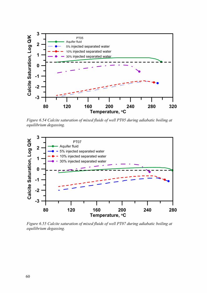
60
80 120 160 200 240 280 320Temperature, oC
-3
-2
-1
0
1
2
3C
alci
te S
atur
atio
n, L
og Q
/K PT05Aquifer fluid
5% injected separated water10% injected separated water30% injected separated water
Figure 6.54 Calcite saturation of mixed fluids of well PT05 during adiabatic boiling at equilibrium degassing.
80 120 160 200 240 280Temperature, oC
-3
-2
-1
0
1
2
3
Cal
cite
Sat
urat
ion,
Log
Q/K PT07
Aquifer fluid5% injected separated water10% injected separated water30% injected separated water
Figure 6.55 Calcite saturation of mixed fluids of well PT07 during adiabatic boiling at equilibrium degassing.
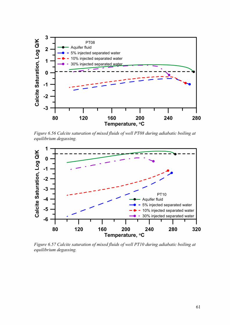
61
80 120 160 200 240 280Temperature, oC
-3
-2
-1
0
1
2
3C
alci
te S
atur
atio
n, L
og Q
/K PT08Aquifer fluid5% injected separated water10% injected separated water30% injected separated water
Figure 6.56 Calcite saturation of mixed fluids of well PT08 during adiabatic boiling at equilibrium degassing.
80 120 160 200 240 280 320Temperature, oC
-6
-5
-4
-3
-2
-1
0
1
Cal
cite
Sat
urat
ion,
Log
Q/K
PT10Aquifer fluid5% injected separated water10% injected separated water30% injected separated water
Figure 6.57 Calcite saturation of mixed fluids of well PT10 during adiabatic boiling at equilibrium degassing.
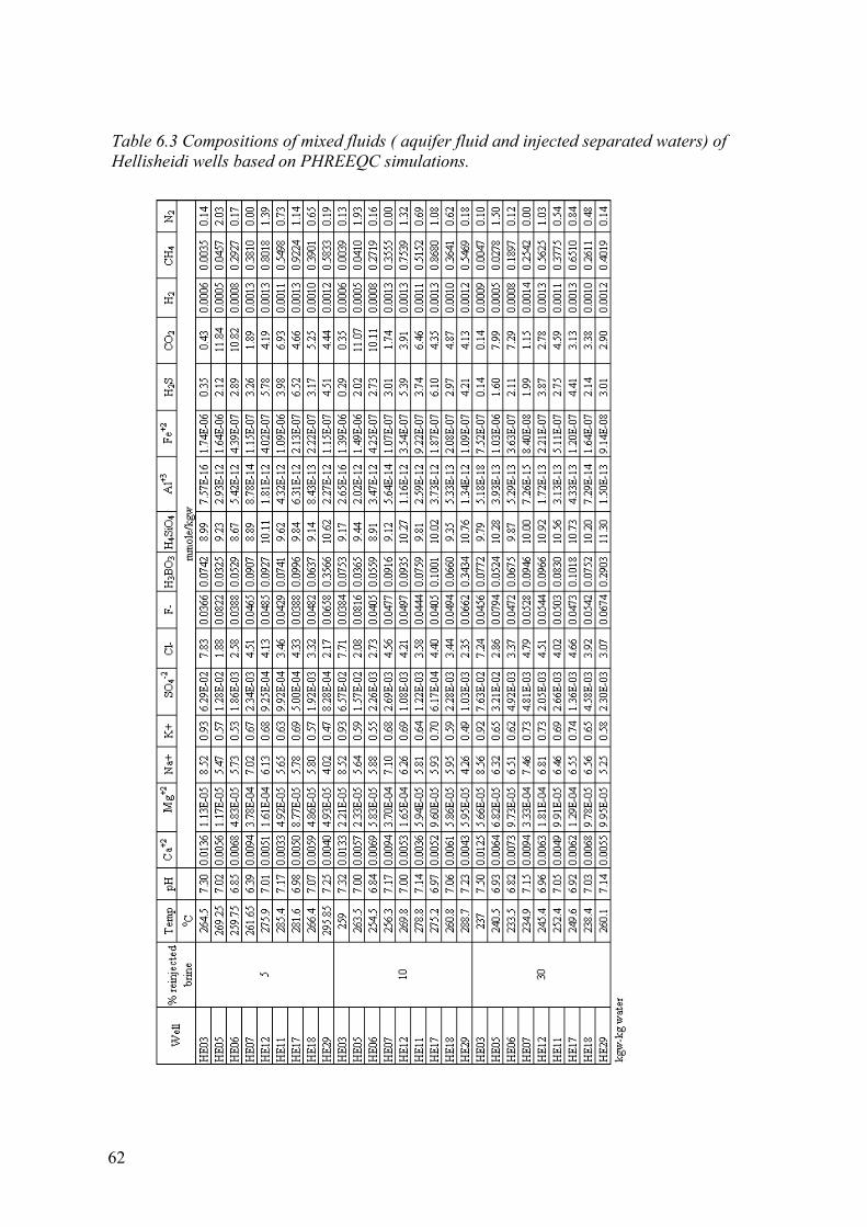
62
Table 6.3 Compositions of mixed fluids ( aquifer fluid and injected separated waters) of Hellisheidi wells based on PHREEQC simulations.
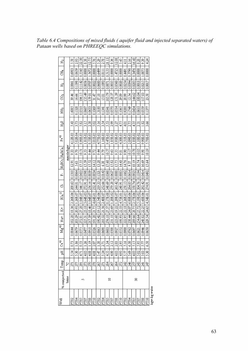
63
Table 6.4 Compositions of mixed fluids ( aquifer fluid and injected separated waters) of Pataan wells based on PHREEQC simulations.

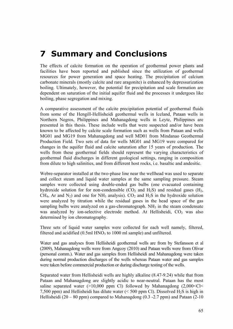
65
7 Summary and Conclusions The effects of calcite formation on the operation of geothermal power plants and facilities have been reported and published since the utilization of geothermal resources for power generation and space heating. The precipitation of calcium carbonate minerals (mostly calcite and rare aragonite) is enhanced by depressurization boiling. Ultimately, however, the potential for precipitation and scale formation are dependent on saturation of the initial aquifer fluid and the processes it undergoes like boiling, phase segregation and mixing.
A comparative assessment of the calcite precipitation potential of geothermal fluids from some of the Hengill-Hellisheidi geothermal wells in Iceland, Pataan wells in Northern Negros, Philippines and Mahanagdong wells in Leyte, Philippines are presented in this thesis. These include wells that were suspected and/or have been known to be affected by calcite scale formation such as wells from Pataan and wells MG01 and MG19 from Mahanagdong and well MD01 from Mindanao Geothermal Production Field. Two sets of data for wells MG01 and MG19 were compared for changes in the aquifer fluid and calcite saturation after 15 years of production. The wells from these geothermal fields should represent the varying characteristics of geothermal fluid discharges in different geological settings, ranging in composition from dilute to high salinities, and from different host rocks, i.e. basaltic and andesitic.
Webre-separator installed at the two-phase line near the wellhead was used to separate and collect steam and liquid water samples at the same sampling pressure. Steam samples were collected using double-ended gas bulbs (one evacuated containing hydroxide solution for for non-condensible (CO2 and H2S) and residual gases (H2, CH4, Ar and N2) and one for NH3 analysis). CO2 and H2S in the hydroxide solution were analyzed by titration while the residual gases in the head space of the gas sampling bulbs were analyzed on a gas-chromatograph. NH3 in the steam condensate was analyzed by ion-selective electrode method. At Hellisheidi, CO2 was also determined by ion chromatography.
Three sets of liquid water samples were collected for each well namely, filtered, filtered and acidified (0.5ml HNO3 to 1000 ml sample) and unfiltered.
Water and gas analyses from Hellisheidi geothermal wells are from by Stefansson et al (2009), Mahanagdong wells were from Angcoy (2010) and Pataan wells were from Olivar (personal comm.). Water and gas samples from Hellisheidi and Mahanagdong were taken during normal production discharges of the wells whereas Pataan water and gas samples were taken before commercial production or during discharge testing of the wells.
Separated water from Hellisheidi wells are highly alkaline (8.47-9.24) while that from Pataan and Mahanagdong are slightly acidic to near-neutral. Pataan has the most saline separated water (>10,000 ppm Cl) followed by Mahanagdong (2,000<Cl< 7,500 ppm) and Hellisheidi has dilute water (< 500 ppm Cl). Dissolved H2S is high in Hellisheidi (20 – 80 ppm) compared to Mahanagdong (0.3 -2.7 ppm) and Pataan (2-10
66
ppm). However, dissolved CO2 in Hellisheidi (4-35 ppm) is lowest compared to Mahanagdong (17-74 ppm) and Pataan (30-68 ppm).
Separated vapour from Pataan wells has the highest CO2 concentration (431-1073 mmol/kg) while Hellisheidi has the lowest concentration (10-155 mmol/kg) and Mahanagdong at the middle (132-628 mmol/kg). Hellisheidi has high H2 gas concentration (up to 34 mmol/kg) compared to Mahanagdong (< 2 mmol/kg) and Pataan (<1 mmol/kg).
Separated water and gas analyses from the wells were used to calculate aquifer fluid compositions using the speciation program WATCH 2.1.
The total discharge SiO2 approaches zero when the total fluid enthalpy approaches that of saturated steam .This is taken to indicate that the “excess” discharge enthalpy of the wells is best explained by phase segregation rather than conductive heating of the fluid by host rock. In addition, Na/K and quartz temperature agree well by the phase segregation model while Na/K temperature are generally higher than quartz for the close system model. Based from these observations it is concluded that “excess” enthalpy is mostly caused by phase segregation in the producing aquifers of Hellisheidi, Mahanagdong and Pataan wells; thus, phase segregation model was used to calculate aquifer compositions.
In this study, the phase segregation temperature was selected to correspond to the vapour saturation pressure at the midpoint between the sampling vapour pressure and the saturation vapour pressure at the selected aquifer temperature. Selected aquifer temperature is based on quartz temperature. The calculation of the aquifer fluid composition was done in two-step run by the speciation program WATCH. Separated water and gas analyses, measured discharge enthalpy and measured pH were used in the first WATCH run which used arbitrary reference temperature equal to the segregation temperature. The output of the first WATCH run was then used as input in the second WATCH run to calculate the initial aquifer fluid composition assuming the flowing fluid to have saturated liquid enthalpy corresponding to the initial aquifer temperature.
The mean percentage differences for quartz and cation geothermometers for individual wells were within 5% (13 oC) except for very high enthalpy wells HE12, HE29 and MG40 and for most of the Pataan wells. No wells exceeded 10% mean percentage differences. The mean percentage difference for all the wells is 4 %. The mean standard deviation of calculated geothermometer temperatures for the wells is 11 oC.
H2S aquifer fluid concentrations of Hellisheidi and Pataan are close to equilibrium with the pyrite-pyrrhotite-magnetite mineral assemblage except HE03 which is significantly below the curve and was found to be highly degassed. Hellisheidi H2S aqueous concentration can also be controlled by pyrite-pyrrhotite-prehnite-epidote mineral assemblage but aqeous H2S concentrations at equilibrium with either of these assemblages are very similar. The data points of Mahanagdong wells are systematically above the equilibrium magnetite-hematite-pyrite mineral assemblage by about 2000J/mol which is within the limit of error according to the data on enthalpy reported by Holland and Powell (1998) on these minerals.
Na/K versus H2S temperatures and quartz versus H2S temperatures of the closed system and phase segregation models show inconsistency for the closed system model but not for the phase segregation model. The geothermometer results for the three
67
study areas substantiate the conclusion that “excess” enthalpy is mostly caused by phase segregation in producing aquifer.
Hellisheidi’s H2 aquifer fluid concentrations were found to be controlled by pyrite-pyrrhotite-magnetite or pyrite-pyrrhotite-prehnite-epidote mineral assemblage. Mahanagdong and Pataan H2 aquifer fluid concentrations on the other hand were found to be controlled by magnetite-hematite mineral assemblage.
Hellisheidi CO2 concentrations were consistently lower than those corresponding to equilibrium while Mahanagdong and Pataan wells were slightly above or at equilibrium with the mineral assemblage clinozoisite-calcite-quartz-prehnite or clinozoisite-calcite-quartz-grossular. One cause of the low CO2 values at Hellisheidi may be insufficient supply of this gas to the fluid.
Aquifer fluid composition calculations show that Hellisheidi’s pH range is alkaline to slightly alkaline (7-7.4) while Mahanagdong’s pH is near neutral around 5.5 (5.3 – 5.9) except for MG40 (pH =4.3) which is a very high enthalpy well. MG40 could be affected by steam condensates or other acidic fluids as it also has the highest concentration of Fe and Mg in Mahanagdong. Pataan wells have slightly acidic pH (4.9 – 5.6).
Hellisheidi wells have higher concentrations of H2 (up to 8 ppm) compared to Mahanagdong and Pataan wells (less than 0.5 ppm). Hellisheidi wells also have higher concentrations of H2S of up to 250 ppm compared to Mahanagdong (<140 ppm) and Pataan (<200 ppm) wells. Pataan wells have the highest CO2 concentration (up to 9700 ppm) followed by Mahanagdong (up to 5300 ppm) while Hellisheidi wells have the lowest (less than 900 ppm).
Chloride-bicarbonate-sulfate ternary diagram of all the wells under study show that Hellisheidi wells are distributed between peripheral water and mature water while most of Mahanagdong and Pataan wells are halfway towards the mature water type.
Na-K-Mg ternary diagram of the wells show that they are discharging partially mixed/ equilibrated to fully equilibrated waters with respect common hydrothermal minerals.
The aquifer fluids are close to equilibrium with calcite and when all uncertainties are taken to account, such as analytical imprecision and selection of aquifer temperatures, departure from saturation are not significant. The average departure from calcite saturation of Hellisheidi wells is only 0.05 SI units, Mahanagdong is 0.2 SI units below the equilibrium while Pataan wells is 0.2 SI units above the equilibrium. Only MG40 well showed high level of undersaturation of 2.1 SI units. MG40 has high “excess” enthalpy and is acidic. Well PT02 is the most oversaturated with 0.74 SI units.
The calculated saturation index for calcite increases with increasing value of the calculated aquifer water pH. This is considered to be due to error in the calculated aquifer water pH. Many factors affect the calculated pH and it is not possible to identify the main sources of apparent variation in pH and calcite saturation index but it seems to be significant, particularly in the case of Hellisheidi.
Mahanagdong and Pataan aquifer fluids approach anhydrite equilibrium whereas Hellisheidi waters are considerably anhydrite undersaturated.
68
At equilibrium, the redox reactions involving pyrite, magnetite, H2S and H2 fixes the aqueous H2S and H2 molal ratios. The Hellisheidi water are quite close to equilibrium, with an average of 0.03 log units above the curve. Mahanagdong and Pataan aquifer waters were systematically with higher H2S/H2 ratios than those corresponding to equilibrium, by 0.2 and 0.55 log units on average, respectively.
The redox reactions involving pyrite, pyrrhotite, H2S and H2 could also fix aqueous H2S and H2 molal ratios. The Hellisheidi aquifer waters are close to equilibrium yet systematically below the equilibrium curve on average by 0.25 log units, if the degassed discharge of HE03and HE05 are excluded. Mahanagdong and Pataan aquifer waters are systematically with higher H2S/H2 ratios than those corresponding to equilibrium, by 0.96 and 1.3 log units on average, respectively. Clearly the H2S/H2 ratios in the aquifer waters in the Philippine geothermal fields are not controlled by the pyrite-pyrrhotite buffer.
An overall pattern in the variation of the saturation index (SI) from Hellisheidi wells with temperature is observed from all the wells except well HE03 upon adiabatic boiling and degassing. The SI initially increases then, after it reaches a peak, decreases to negative values. The initial increase in SI reflects an increase in pH due to CO2 and H2S degassing. The pH increase caused a strong increase in the activity of the CO3
−2 species. At maximum SI values, the water has been largely degassed, and the subsequent decline in SI is caused by increased calcite solubility with decreasing temperature. Well HE03 is highly degassed as reflected by the low gas content of the discharge. Boiling of the degassed water causes a decrease in the value of SI. The extent of degassing (as expressed by the degassing coefficient) increases the level of calcite SI except for degassed well HE03 which showed the opposite.
The majority of the wells in Mahanagdong followed the general pattern exhibited by Hellisheidi wells except MG40, MG29, MG14 and MG03. MG40 is a high “excess” enthalpy and is acidic. MG03 and MG14 were postulated to receive fluid from the upflow zone but have been affected by brine injection returns. The reservoir chloride levels of MG03 and MG14 are shifted towards the composition of the injected brine. Well MG29, on the other hand, is located in the western periphery of the Mahanagdong geothermal system and could be affected by intrusion of cooler peripheral waters. The highest positive departure from the initial saturation in Mahanagdong is from MG19, with 0.40 (at 251 oC) SI units above the initial saturation at maximum degassing Calcite scale is known to form in MG19.
Boiling of MG01 aquifer fluid sampled in 1994 produces an increase in calcite saturation of 0.51 SI units above the initial saturation which is high compared to the more recent sample with only 0.07 SI units departure from the initial saturation. Comparing MG01 CO2 and H2S concentrations on samples taken in 2009 and 1994 shows that it has been partially degassed or mixed with degassed injected brine. Aquifer aqueous CO2 concentration decreased from 8000 to 1200 ppm and H2S concentration decreased from 92 to 15 ppm. Activity of free Ca2+ probably affects calcite saturation because it partially increased from 10 to 16 ppm in 1994 to 2009 samples.
The case of MG19 is similar with MG01. The present fluid discharge is partially degassed or mixed with injected brine and Ca2+ concentration has increased. Aquifer aqueous CO2 concentration decreased from 6900 to 3200 ppm, aqueous H2S
69
concentration decreased from 71 to 36 ppm and Ca2+ increased from 11 to 20 ppm. Calcite mineral SI trend of MG19 practically remains the same after almost 15 years of production, though the old data showed a higher departure of 0.48 SI units above the initial saturation compared to 0.40 SI units for the more recent sample.
Pataan aquifer fluids show trends similar to those of Hellisheidi and most of the Mahanagdong wells. Well PT08 shows the highest increase in the SI for calcite of 0.6 units (at 223 oC) above the initial saturation, followed by PT05, PT10 and PT07 with 0.40 (at 246 oC), 0.31(at 258 oC) and 0.28 (at 252 oC) SI units above the the initial saturation, respectively. PT05 was postulated to be nearest to the upflow region, followed by PT08 and PT07. Well PT05 has the highest dissolved aqueous CO2 concentration at 9700 ppm followed by PT08 and PT07 at 7800 and 6700 ppm, respectively.
Wells PT02 and PT04 have the lowest positive departure from the initial saturation at 0.10 (at 262 oC) and 0.15 (at 262 oC) SI units above the initial saturation, respectively.
The implications for Pataan of the above described observations are that 1) the aquifer fluid feeding PT05 and PT08 may precipitate calcite in the immediate aquifer formation and in the well when degassing is more than 50% 2) aquifer fluids feeding PT10 and PT07 may precipitate calcite in the aquifer if sufficient over-saturation is produced and 3) aquifer fluid feeding PT02 may precipitate calcite in the well and/or in the aquifer if the degassing is less than 50% of maximum.
It has been reported that PT02 is the only well that has physical evidence of calcite scale formation in the well. However, field-wide decline in total mass flow in the wells were documented during commissioning activities in 2007 that may be caused by calcite precipitation in producing aquifers.
The effect of boiling and degassing on calcite saturation for the one well from Mindanao Geothermal Production Field, MD01, is similar to Hellisheidi and Mahanagdong wells. It has highest departure of 0.425 SI units above the initial saturation at 241.5 oC and maximum degassing. This well is thought to be affected by calcite scaling.
The effect of fluid mixing particularly the injected separated water from the separators and aquifer fluids from Hellisheidi and Pataan areas were investigated. Pataan separated water is slightly acid, pH of 5.3 and higher in dissolved CO2 than Hellisheidi. Hellisheidi separated water on the other hand is very alkaline with pH of 9.3 and has higher H2S concentration than Pataan. Pataan separated water is being injected at temperature of 160 oC, which is used in both Pataan and Hellisheidi mixing simulations. The composition of the fluid mixtures were simulated using the aqueous modeling code PHREEQC-2 version 2.17.00 from the graphical interface PHREEQC for Windows. The mixed fluid compositions were then inputted into WATCH 2.1 to simulate boiling and degassing.
The results show that calcite saturation of the mixed fluids dropped to below the initial saturation of aquifer fluids. Increasing the injected separated water proportion in the mixture decreases the calcite saturation index of the mixed fluid for the case of Hellisheidi wells. In Pataan wells, however, increasing the separated water proportion in the mixture increases the calcite SI of the mixed fluid.

70
In Hellisheidi, the calcite saturation index of the mixed fluid upon boiling are below that of the initial aquifer fluid except HE11 where at 30% mix injected separated water, the saturation approach that of the initial aquifer fluid saturation. In Pataan, it seems that mixing injected separated water by more than 30% of the initial aquifer fluids will bring the saturation to or above the initial saturation upon adiabatic boiling.
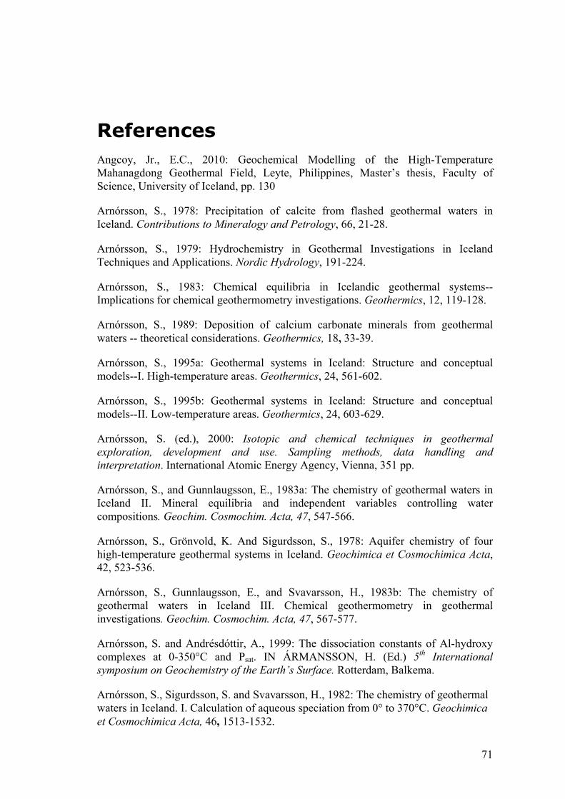
71
References Angcoy, Jr., E.C., 2010: Geochemical Modelling of the High-Temperature Mahanagdong Geothermal Field, Leyte, Philippines, Master’s thesis, Faculty of Science, University of Iceland, pp. 130
Arnórsson, S., 1978: Precipitation of calcite from flashed geothermal waters in Iceland. Contributions to Mineralogy and Petrology, 66, 21-28.
Arnórsson, S., 1979: Hydrochemistry in Geothermal Investigations in Iceland Techniques and Applications. Nordic Hydrology, 191-224.
Arnórsson, S., 1983: Chemical equilibria in Icelandic geothermal systems--Implications for chemical geothermometry investigations. Geothermics, 12, 119-128.
Arnórsson, S., 1989: Deposition of calcium carbonate minerals from geothermal waters -- theoretical considerations. Geothermics, 18, 33-39.
Arnórsson, S., 1995a: Geothermal systems in Iceland: Structure and conceptual models--I. High-temperature areas. Geothermics, 24, 561-602.
Arnórsson, S., 1995b: Geothermal systems in Iceland: Structure and conceptual models--II. Low-temperature areas. Geothermics, 24, 603-629.
Arnórsson, S. (ed.), 2000: Isotopic and chemical techniques in geothermal exploration, development and use. Sampling methods, data handling and interpretation. International Atomic Energy Agency, Vienna, 351 pp.
Arnórsson, S., and Gunnlaugsson, E., 1983a: The chemistry of geothermal waters in Iceland II. Mineral equilibria and independent variables controlling water compositions. Geochim. Cosmochim. Acta, 47, 547-566.
Arnórsson, S., Grönvold, K. And Sigurdsson, S., 1978: Aquifer chemistry of four high-temperature geothermal systems in Iceland. Geochimica et Cosmochimica Acta, 42, 523-536.
Arnórsson, S., Gunnlaugsson, E., and Svavarsson, H., 1983b: The chemistry of geothermal waters in Iceland III. Chemical geothermometry in geothermal investigations. Geochim. Cosmochim. Acta, 47, 567-577.
Arnórsson, S. and Andrésdóttir, A., 1999: The dissociation constants of Al-hydroxy complexes at 0-350°C and Psat. IN ÁRMANSSON, H. (Ed.) 5th International symposium on Geochemistry of the Earth’s Surface. Rotterdam, Balkema.
Arnórsson, S., Sigurdsson, S. and Svavarsson, H., 1982: The chemistry of geothermal waters in Iceland. I. Calculation of aqueous speciation from 0° to 370°C. Geochimica et Cosmochimica Acta, 46, 1513-1532.
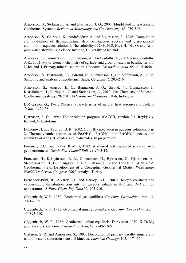
72
Arnórsson, S., Stefansson, A. and Bjarnason, J. O., 2007: Fluid-Fluid Interactions in Geothermal Systems. Reviews in Mineralogy and Geochemistry, 65, 259-312.
Arnórsson, S., Geirsson, K., Andrésdóttir, A. and Sigurdsson, S., 1996: Compilation and evaluation of thermodynamic data on aqueous species and dissociational equilibria in aqueous solution I. The solubility of CO2, H2S, H2, CH4, N2, O2 and Ar in pure water. Reykjavik, Science Institute, University of Iceland.
Arnórsson, S., Gunnarsson, I., Stefánsson, A., Andrésdóttir, A., and Sveinbjörnsdóttir, A.E., 2002: Major element chemistry of surface- and ground waters in basaltic terrain, N-Iceland. I. Primary mineral saturation. Geochim. Cosmochim. Acta, 66, 4015-4046.
Arnórsson, S., Bjarnason, J.Ö., Giroud, N., Gunnarsson, I., and Stefánsson, A., 2006: Sampling and analysis of geothermal fluids, Geofluids, 6, 203-216.
Arnórsson, S., Angcoy, E. C., Bjarnason, J. Ö., Giroud, N., Gunnarsson, I., Kaasalainen, H., Karingithi, C. and Stefánsson, A., 2010: Gas Chemistry of Volcanic Geothermal Systems. 2010 World Geothermal Congress. Bali, Indonesia.
Böðvarsson, G., 1961: Physical characteristics of natural heat resources in Iceland Jökull 11, 29-38.
Bjarnason, J. Ö., 1994: The speciation program WATCH, version 2.1. Reykjavik, Iceland, Orkustofnun.
Diakonov, I. and Tagirov, B. R., 2002: Iron (III) speciation in aqueous solutions: Part 2. Thermodynamic properties of Fe(OH)+2, Fe(OH)+2 and Fe(OH)3° species and solubility of iron (III) oxides, and hydroxides. In preparation.
Fournier, R.O., and Potter, R.W. II, 1982: A revised and expanded silica (quartz) geothermometer. Geoth. Res. Council Bull.,11-10, 3-12.
Franzson, H., Kristjánsson, B. R., Gunnarsson, G., Björnsson, G., Hjartarson, A., Steingrímsson, B., Gunnlaugsson, E. and Gíslason, G., 2005: The Hengill-Hellisheiði Geothermal Field. Development of a Conceptual Geothermal Model. Proceedings World Geothermal Congress 2005. Antalya, Turkey.
Fernandez-Prini, R., Alvarez, J.L. and Harvey, A.H., 2003: Henry’s constants and vapour-liquid distribution constants for gaseous solutes in H2O and D2O at high temperatures. J. Phys. Chem. Ref. Data 32, 903-916.
Giggenbach, W.F., 1980: Geothermal gas equilibria. Geochim. Cosmochim. Acta, 44, 2021-2032.
Giggenbach, W.F., 1981: Geothermal mineral equilibria. Geochim. Cosmochim. Acta, 45, 393-410.
Giggenbach, W. F., 1988: Geothermal solute equilibria. Derivation of Na-K-Ca-Mg geoindicators. Geochim. Cosmochim. Acta, 52: 2749-2765.
Gislason, S. R. and Arnórsson, S., 1993: Dissolution of primary basaltic minerals in natural waters: saturation state and kinetics. Chemical Geology, 105, 117-135.
73
Gudmundsson, B. T. and Arnórsson, S., 2005: Secondary mineral-fluid equilibria in the Krafla and Námafjall geothermal systems, Iceland. Applied Geochemistry, 20, 1607-1625.
Gunnarsson, I. and Arnórsson, S., 2000: Amorphous silica solubility and the thermodynamic properties of H4SiO4
° in the range of 0° to 350°C at Psat. Geochimica et Cosmochimica Acta, 64, 2295-2307.
Gunnarsson, I. and Arnórsson, S., 2005: Impact of silica scaling on the efficiency of heat extraction from high-temperature geothermal fluids. Geothermics, 34, 320-329.
Holland, T. J. B. and Powell, R., 1998: An internally consistent thermodynamic data set for phases of petrological interest. J. metamorphic Geol, 16, 309-344.
Karingithi, C.W., Arnórsson, S., and Grönvold, K., 2010: Processes controlling aquifer fluid compositions in the Olkaria geothermal system, Kenya. J. Volc. Geothermal Res. (in press).
Mutonga, M. W., 2007: The Isotopic and Chemical Characteristics of Geothermal Fluids In Hengill Area, Sw-Iceland: Hellisheidi, Hveragerdi And Nesjavellir Fields. Reykjavik, Iceland, United Nations University - Geothermal Training Programme.
Olivar, M. V. M., 2007: The Geochemistry of Northern Negros Geothermal Production Field. Taguig City, Philippines, Energy Development Corporation. Internal report (unpublished).
Parkhurst, D. L. and Appelo, C. A. J., 1999: User’s guide to PHREEQC (Version2)-A computer program for speciation, batch-reaction, one-dimensional transport, and inverse geochemical calculations U.S.Geological Survey Water-Resources Investigations Report 99-4259.
Parkhurst, D. L., Thorstenson, D. C. and Plummer, L. N., 1980: PHREEQE--A computer program for geochemical calculations. U.S. Geological Survey Investigations Report 80-96.
Pokrovski, G. S., Schott, J., Salvi, G., Gout, R. and Kubicki, J. D., 1998: Structure and stability of aluminium-silica complexes in neutral to basic solutions. Experimental study and molecular orbital calculations. Min. Mag., 62A, 1194-1195.
Rahmani, M. R., 2007: Assessment Of Calcite Scaling Potential In The Geothermal Wells Of The Nw-Sabalan Geothermal Prospect, Nw-Iran. Reykjavik City, Iceland, United Nations University - Geothermal Training Programme.
Robie, R.A. and Hemmingway, B.S., 1995: Thermodynamic properties of minerals and related substances at 298.15 K and 1 bar (105 Pascals) pressures and at higher temperatures. USGS. Bull. 2131, 461p.
Salonga, N. D., Dacillo, D. B. and Siega, F. L., 2004: Providing solutions to the rapid changes induced by stressed production in Mahanagdong geothermal field, Philippines. Geothermics, 33, 181-212.
74
Sanchez, D. R., Baltasar, A. S. J. and Candelaria, M. N. R., 2005: Evaluation of Chemical Equilibria of Calcite Deposition in a Geothermal Well at Northern Negros Geothermal Project, Philippines. Proceedings World Geothermal Congress 2005. Antalya, Turkey.
Satman, A., Ugur, Z. and Onur, M., 1999: The effect of calcite deposition on geothermal well inflow performance. Geothermics, 28, 425-444.
Siega, F. L., Herras, E. B. and Buñing, B. C., 2005: Calcite Scale Inhibition: The Case of Mahanagdong Wells in Leyte Geothermal Production Field, Philippines. Proceedings World Geothermal Congress 2005. Anatalya,Turkey.
Stáhl, G., Pátzay, G., Weiser, L. and Kálmán, E., 2000: Study of calcite scaling and corrosion processes in geothermal systems. Geothermics, 29, 105-119.
Stefánsson, A., 2001: Dissolution of primary minerals of basalt in natural waters: I. Calculation of mineral solubilities from 0°C to 350°C. Chemical Geology, 172, 225-250.
Stefánsson, A., Gíslason, S. R. and Arnórsson, S., 2001: Dissolution of primary minerals in natural waters: II. Mineral saturation state. Chemical Geology, 172, 251-276.
Stefánsson, A. and Arnórsson, S., 2002: Gas pressures and redox reactions in geothermal fluids in Iceland. Chemical Geology, 190, 251-271.
Stefánsson, A., Gunnarsson, I., and Giroud, N., 2007: New methods for the direct determination of dissolved inorganic, organic and total carbon in natural waters by Reagent-Free TM Ion Chromatography and inductively coupled plasma atomic emission spectrometry. Analytical Chimica Acta, 582, 69-72.
Tole, M. P., Ármannsson, H., Zhong-He, P. and Arnórsson, S., 1993: Fluid/mineral equilibrium calculations for geothermal fluids and chemical geothermometry. Geothermics, 22, 17-37.
Urbino, G.A. and Zhong-He, P., 2006: 2003 Inter-laboratory comparison of geothermal water chemistry. In: Zhong-He, P., and, Ármansson, H. (eds.), Analytical procedures and quality assurance for geothermal water chemistry. UNU-GTP, Reykjavik, Iceland, 131-172.
Zhong-He, P. and Ármansson, H., 2006: Analytical procedures and quality assurance for geothermal water chemistry. Reykjavik City, Iceland, United Nations University - Geothermal Training Programme.
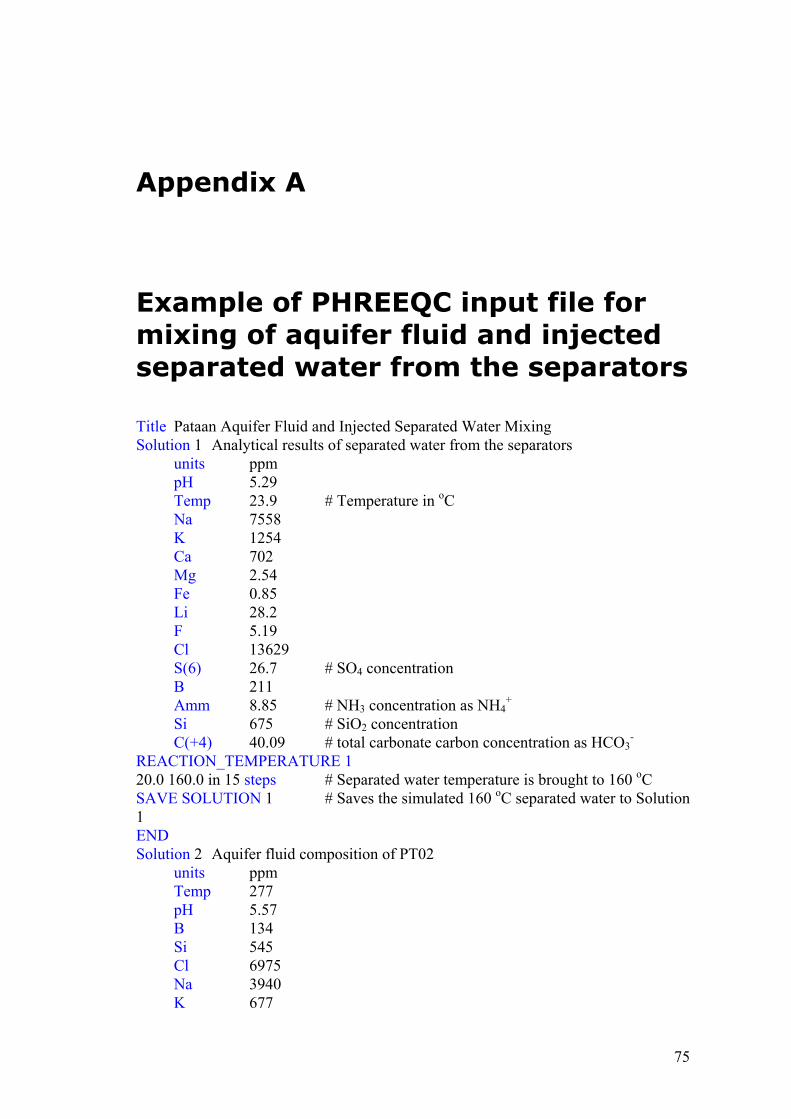
75
Appendix A
Example of PHREEQC input file for mixing of aquifer fluid and injected separated water from the separators Title Pataan Aquifer Fluid and Injected Separated Water Mixing Solution 1 Analytical results of separated water from the separators units ppm pH 5.29 Temp 23.9 # Temperature in oC Na 7558 K 1254 Ca 702 Mg 2.54 Fe 0.85 Li 28.2 F 5.19 Cl 13629 S(6) 26.7 # SO4 concentration B 211 Amm 8.85 # NH3 concentration as NH4
+ Si 675 # SiO2 concentration C(+4) 40.09 # total carbonate carbon concentration as HCO3
-
REACTION_TEMPERATURE 1 20.0 160.0 in 15 steps # Separated water temperature is brought to 160 oC SAVE SOLUTION 1 # Saves the simulated 160 oC separated water to Solution 1 END Solution 2 Aquifer fluid composition of PT02
units ppm Temp 277 pH 5.57 B 134 Si 545 Cl 6975 Na 3940 K 677
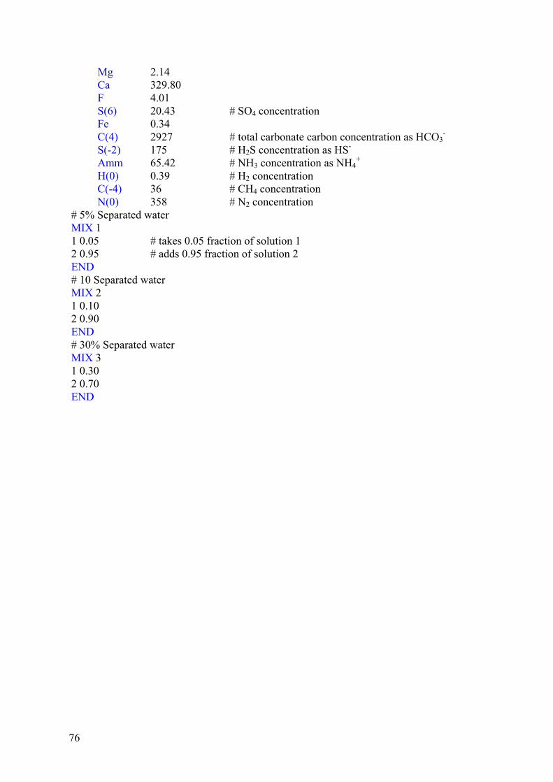
76
Mg 2.14 Ca 329.80 F 4.01 S(6) 20.43 # SO4 concentration Fe 0.34 C(4) 2927 # total carbonate carbon concentration as HCO3
-
S(-2) 175 # H2S concentration as HS- Amm 65.42 # NH3 concentration as NH4
+ H(0) 0.39 # H2 concentration C(-4) 36 # CH4 concentration N(0) 358 # N2 concentration
# 5% Separated water MIX 1 1 0.05 # takes 0.05 fraction of solution 1 2 0.95 # adds 0.95 fraction of solution 2 END # 10 Separated water MIX 2 1 0.10 2 0.90 END # 30% Separated water MIX 3 1 0.30 2 0.70 END