
CalcI Complete Solutions
615
CALCULUS I Solutions to Practice Problems Paul Dawkins
-
Upload
jorden-senior -
Category
Documents
-
view
168 -
download
4
Transcript of CalcI Complete Solutions

CALCULUS I Solutions to Practice Problems
Paul Dawkins
Calculus I
© 2007 Paul Dawkins i http://tutorial.math.lamar.edu/terms.aspx
Table of Contents Preface ............................................................................................................................................. 2 Review ............................................................................................................................................. 2
Review : Functions.................................................................................................................................... 3 Review : Inverse Functions .................................................................................................................... 26 Review : Trig Functions .......................................................................................................................... 35 Review : Solving Trig Equations ............................................................................................................ 52 Review : Solving Trig Equations with Calculators, Part I .................................................................... 81 Review : Solving Trig Equations with Calculators, Part II ................................................................. 103 Review : Exponential Functions .......................................................................................................... 119 Review : Logarithm Functions ............................................................................................................. 123 Review : Exponential and Logarithm Equations ................................................................................ 131 Review : Common Graphs .................................................................................................................... 149
Limits .......................................................................................................................................... 166 Rates of Change and Tangent Lines ..................................................................................................... 166 The Limit ............................................................................................................................................... 176 One-Sided Limits................................................................................................................................... 184 Limit Properties .................................................................................................................................... 191 Computing Limits ................................................................................................................................. 200 Infinite Limits ........................................................................................................................................ 207 Limits At Infinity, Part I ........................................................................................................................ 220 Limits At Infinity, Part II....................................................................................................................... 232 Continuity .............................................................................................................................................. 239 The Definition of the Limit ................................................................................................................... 254
Derivatives .................................................................................................................................. 254 The Definition of the Derivative .......................................................................................................... 254 Interpretations of the Derivative ......................................................................................................... 263 Differentiation Formulas ...................................................................................................................... 279 Product and Quotient Rule ................................................................................................................... 292 Derivatives of Trig Functions .............................................................................................................. 298 Derivatives of Exponential and Logarithm Functions ....................................................................... 304 Derivatives of Inverse Trig Functions ................................................................................................. 309 Derivatives of Hyperbolic Functions ................................................................................................... 310 Chain Rule ............................................................................................................................................. 311 Implicit Differentiation......................................................................................................................... 331 Related Rates ........................................................................................................................................ 340 Higher Order Derivatives ..................................................................................................................... 353 Logarithmic Differentiation ................................................................................................................. 360
Applications of Derivatives ....................................................................................................... 364 Rates of Change ..................................................................................................................................... 364 Critical Points ........................................................................................................................................ 364 Minimum and Maximum Values .......................................................................................................... 378 Finding Absolute Extrema.................................................................................................................... 389 The Shape of a Graph, Part I ................................................................................................................. 405 The Shape of a Graph, Part II ............................................................................................................... 428 The Mean Value Theorem .................................................................................................................... 456 Optimization ......................................................................................................................................... 461 More Optimization Problems............................................................................................................... 474 Indeterminate Forms and L’Hospital’s Rule ....................................................................................... 489 Linear Approximations ........................................................................................................................ 503 Differentials........................................................................................................................................... 507 Newton’s Method .................................................................................................................................. 510 Business Applications .......................................................................................................................... 521
Calculus I
© 2007 Paul Dawkins ii http://tutorial.math.lamar.edu/terms.aspx
Integrals ...................................................................................................................................... 526 Indefinite Integrals ............................................................................................................................... 526 Computing Indefinite Integrals............................................................................................................ 530 Substitution Rule for Indefinite Integrals ........................................................................................... 544 More Substitution Rule ........................................................................................................................ 561 Area Problem ........................................................................................................................................ 574 The Definition of the Definite Integral ................................................................................................ 581 Computing Definite Integrals ............................................................................................................... 589 Substitution Rule for Definite Integrals .............................................................................................. 603
Applications of Integrals ........................................................................................................... 613 Average Function Value ....................................................................................................................... 613 Area Between Curves ........................................................................................................................... 613 Volumes of Solids of Revolution / Method of Rings ........................................................................... 613 Volumes of Solids of Revolution / Method of Cylinders .................................................................... 613 More Volume Problems ........................................................................................................................ 613 Work ...................................................................................................................................................... 613
Preface Here are the solutions to the practice problems for my Calculus I notes. Some solutions will have more or less detail than other solutions. The level of detail in each solution will depend up on several issues. If the section is a review section, this mostly applies to problems in the first chapter, there will probably not be as much detail to the solutions given that the problems really should be review. As the difficulty level of the problems increases less detail will go into the basics of the solution under the assumption that if you’ve reached the level of working the harder problems then you will probably already understand the basics fairly well and won’t need all the explanation. This document was written with presentation on the web in mind. On the web most solutions are broken down into steps and many of the steps have hints. Each hint on the web is given as a popup however in this document they are listed prior to each step. Also, on the web each step can be viewed individually by clicking on links while in this document they are all showing. Also, there are liable to be some formatting parts in this document intended for help in generating the web pages that haven’t been removed here. These issues may make the solutions a little difficult to follow at times, but they should still be readable.
Review

Calculus I
© 2007 Paul Dawkins 3 http://tutorial.math.lamar.edu/terms.aspx
Review : Functions 1. Perform the indicated function evaluations for ( ) 23 5 2f x x x= − − .
(a) ( )4f (b) ( )0f (c) ( )3f −
(d) ( )6f t− (e) ( )7 4f x− (f) ( )f x h+
(a) ( )4f [Solution]
( ) ( ) ( )24 3 5 4 2 4 49f = − − = − (b) ( )0f [Solution]
( ) ( ) ( )20 3 5 0 2 0 3f = − − = (c) ( )3f − [Solution]
( ) ( ) ( )23 3 5 3 2 3 0f − = − − − − = Hint : Don’t let the fact that there are now variables here instead of numbers get you confused. This works exactly the same way as the first three it will just have a little more algebra involved. (d) ( )6f t− [Solution]
( ) ( ) ( )( ) ( )
2
2
2
2
6 3 5 6 2 6
3 5 6 2 36 12
3 30 5 72 24 299 29 2
f t t t
t t t
t t tt t
− = − − − −
= − − − − +
= − + − + −
= − + −
Hint : Don’t let the fact that there are now variables here instead of numbers get you confused. This works exactly the same way as the first three it will just have a little more algebra involved. (e) ( )7 4f x− [Solution]
( ) ( ) ( )( ) ( )
2
2
2
2
7 4 3 5 7 4 2 7 4
3 5 7 4 2 49 56 16
3 35 20 98 112 32130 132 32
f x x x
x x x
x x xx x
− = − − − −
= − − − − +
= − + − + −
= − + −
Hint : Don’t let the fact that there are now variables here instead of numbers get you confused. Also, don’t get excited about the fact that there is both an x and an h here. This works exactly the same way as the first three it will just have a little more algebra involved.
Calculus I
© 2007 Paul Dawkins 4 http://tutorial.math.lamar.edu/terms.aspx
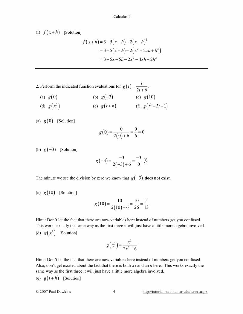
(f) ( )f x h+ [Solution]
( ) ( ) ( )( ) ( )
2
2 2
2 2
3 5 2
3 5 2 2
3 5 5 2 4 2
f x h x h x h
x h x xh h
x h x xh h
+ = − + − +
= − + − + +
= − − − − −
2. Perform the indicated function evaluations for ( )2 6
tg tt
=+
.
(a) ( )0g (b) ( )3g − (c) ( )10g
(d) ( )2g x (e) ( )g t h+ (f) ( )2 3 1g t t− +
(a) ( )0g [Solution]
( ) ( )0 00 0
2 0 6 6g = = =
+
(b) ( )3g − [Solution]
( ) ( )3 33
2 3 6 0g − −
− = =− +
The minute we see the division by zero we know that ( )3g − does not exist.
(c) ( )10g [Solution]
( ) ( )10 10 510
2 10 6 26 13g = = =
+
Hint : Don’t let the fact that there are now variables here instead of numbers get you confused. This works exactly the same way as the first three it will just have a little more algebra involved.
(d) ( )2g x [Solution]
( )2
222 6xg x
x=
+
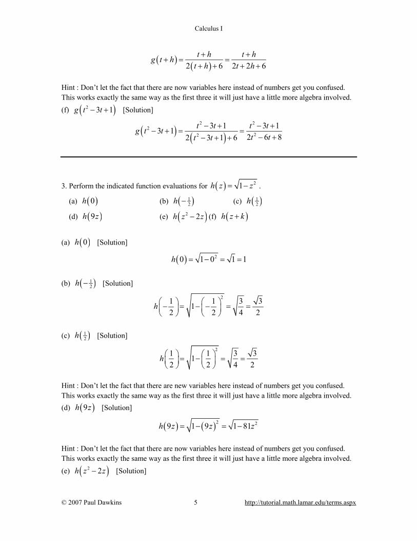
Hint : Don’t let the fact that there are now variables here instead of numbers get you confused. Also, don’t get excited about the fact that there is both a t and an h here. This works exactly the same way as the first three it will just have a little more algebra involved. (e) ( )g t h+ [Solution]
Calculus I
© 2007 Paul Dawkins 5 http://tutorial.math.lamar.edu/terms.aspx
( ) ( )2 6 2 2 6t h t hg t h
t h t h+ +
+ = =+ + + +
Hint : Don’t let the fact that there are now variables here instead of numbers get you confused. This works exactly the same way as the first three it will just have a little more algebra involved.
(f) ( )2 3 1g t t− + [Solution]
( ) ( )2 2
222
3 1 3 13 12 6 82 3 1 6
t t t tg t tt tt t
− + − +− + = =
− +− + +
3. Perform the indicated function evaluations for ( ) 21h z z= − .
(a) ( )0h (b) ( )12h − (c) ( )1
2h
(d) ( )9h z (e) ( )2 2h z z− (f) ( )h z k+
(a) ( )0h [Solution]
( ) 20 1 0 1 1h = − = = (b) ( )1
2h − [Solution]
21 1 3 31
2 2 4 2h − = − − = =
(c) ( )1
2h [Solution]
21 1 3 31
2 2 4 2h = − = =
Hint : Don’t let the fact that there are new variables here instead of numbers get you confused. This works exactly the same way as the first three it will just have a little more algebra involved. (d) ( )9h z [Solution]
( ) ( )2 29 1 9 1 81h z z z= − = − Hint : Don’t let the fact that there are now variables here instead of numbers get you confused. This works exactly the same way as the first three it will just have a little more algebra involved.
(e) ( )2 2h z z− [Solution]

Calculus I
© 2007 Paul Dawkins 6 http://tutorial.math.lamar.edu/terms.aspx
( ) ( ) ( )22 2 4 3 2 2 3 42 1 2 1 4 4 1 4 4h z z z z z z z z z z− = − − = − − + = − + − Hint : Don’t let the fact that there are now variables here instead of numbers get you confused. Also, don’t get excited about the fact that there is both a z and a k here. This works exactly the same way as the first three it will just have a little more algebra involved. (f) ( )h z k+ [Solution]
( ) ( ) ( )2 2 2 2 21 1 2 1 2h z k z k z zk k z zk k+ = − + = − + + = − − −
4. Perform the indicated function evaluations for ( ) 431
R x xx
= + −+
.
(a) ( )0R (b) ( )6R (c) ( )9R −
(d) ( )1R x + (e) ( )4 3R x − (f) ( )1 1xR −
(a) ( )0R [Solution]
( ) 40 3 0 3 40 1
R = + − = −+
(b) ( )6R [Solution]
( ) 4 4 4 176 3 6 9 36 1 7 7 7
R = + − = − = − =+
(c) ( )9R − [Solution]
( ) ( ) 4 49 3 9 69 1 8
R − = + − − = − −− + −
In this class we only deal with functions that give real values as answers. Therefore, because we have the square root of a negative number in the first term this function is not defined. Note that the fact that the second term is perfectly acceptable has no bearing on the fact that the function will not be defined here. If any portion of the function is not defined upon evaluation then the whole function is not defined at that point. Also note that if we allow complex numbers this function will be defined. Hint : Don’t let the fact that there are now variables here instead of numbers get you confused. This works exactly the same way as the first three it will just have a little more algebra involved. (d) ( )1R x + [Solution]

Calculus I
© 2007 Paul Dawkins 7 http://tutorial.math.lamar.edu/terms.aspx
( ) ( ) ( )4 41 3 1 41 1 2
R x x xx x
+ = + + − = + −+ + +
Hint : Don’t let the fact that there are now variables here instead of numbers get you confused. This works exactly the same way as the first three it will just have a little more algebra involved.
(e) ( )4 3R x − [Solution]
( ) ( ) ( )4 4 4 2
4 44
4 4 43 3 32 23 1
R x x x xx xx
− = + − − = − = −− −− +
Hint : Don’t let the fact that there are now variables here instead of numbers get you confused. This works exactly the same way as the first three it will just have a little more algebra involved. (f) ( )1 1xR − [Solution]
( ) 11
1 1 4 1 4 11 3 1 2 2 41 1 xx
R xx x x x
− = + − − = + − = + − − +
5. The difference quotient of a function ( )f x is defined to be,
( ) ( )f x h f xh
+ −
compute the difference quotient for ( ) 4 9f x x= − .
Hint : Compute ( )f x h+ , then compute the numerator and finally compute the difference
quotient. Step 1 ( ) ( )4 9 4 4 9f x h x h x h+ = + − = + − Step 2 ( ) ( ) ( )4 4 9 4 9 4f x h f x x h x h+ − = + − − − = Step 3
( ) ( ) 4 4f x h f x h
h h+ −
= =

Calculus I
© 2007 Paul Dawkins 8 http://tutorial.math.lamar.edu/terms.aspx
6. The difference quotient of a function ( )f x is defined to be,
( ) ( )f x h f xh
+ −
compute the difference quotient for ( ) 26g x x= − .
Hint : Don’t get excited about the fact that the function is now named ( )g x , the difference
quotient still works in the same manner it just has g’s instead of f’s now. So, compute ( )g x h+ ,
then compute the numerator and finally compute the difference quotient. Step 1
( ) ( )2 2 26 6 2g x h x h x xh h+ = − + = − − − Step 2
( ) ( ) ( )2 2 2 26 2 6 2g x h g x x xh h x xh h+ − = − − − − − = − − Step 3
( ) ( ) 22 2g x h g x xh h x h
h h+ − − −
= = − −
7. The difference quotient of a function ( )f x is defined to be,
( ) ( )f x h f xh
+ −
compute the difference quotient for ( ) 22 3 9f t t t= − + .
Hint : Don’t get excited about the fact that the function is now ( )f t , the difference quotient still
works in the same manner it just has t’s instead of x’s now. So, compute ( )f t h+ , then compute
the numerator and finally compute the difference quotient. Step 1
( ) ( ) ( ) ( )2 2 2
2 2
2 3 9 2 2 3 3 9
2 4 2 3 3 9
f t h t h t h t th h t h
t th h t h
+ = + − + + = + + − − +
= + + − − +
Step 2
( ) ( ) ( )2 2 2 22 4 2 3 3 9 2 3 9 4 2 3f t h f t t th h t h t t th h h+ − = + + − − + − − + = + −
Calculus I
© 2007 Paul Dawkins 9 http://tutorial.math.lamar.edu/terms.aspx
Step 3
( ) ( ) 24 2 3 4 2 3f t h f t th h h t h
h h+ − + −
= = + −
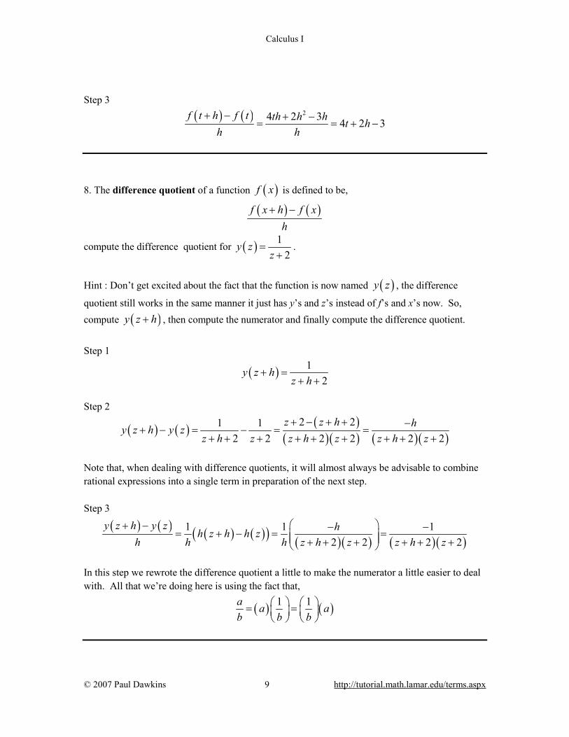
8. The difference quotient of a function ( )f x is defined to be,
( ) ( )f x h f xh
+ −
compute the difference quotient for ( ) 12
y zz
=+
.
Hint : Don’t get excited about the fact that the function is now named ( )y z , the difference
quotient still works in the same manner it just has y’s and z’s instead of f’s and x’s now. So, compute ( )y z h+ , then compute the numerator and finally compute the difference quotient.
Step 1
( ) 12
y z hz h
+ =+ +
Step 2
( ) ( ) ( )( )( ) ( )( )
2 21 12 2 2 2 2 2
z z h hy z h y zz h z z h z z h z
+ − + + −+ − = − = =
+ + + + + + + + +
Note that, when dealing with difference quotients, it will almost always be advisable to combine rational expressions into a single term in preparation of the next step. Step 3
( ) ( ) ( ) ( )( ) ( )( ) ( ) ( )1 1 1
2 2 2 2y z h y z hh z h h z
h h h z h z z h z + − − −
= + − = = + + + + + +
In this step we rewrote the difference quotient a little to make the numerator a little easier to deal with. All that we’re doing here is using the fact that,
( ) ( )1 1a a ab b b
= =
Calculus I
© 2007 Paul Dawkins 10 http://tutorial.math.lamar.edu/terms.aspx
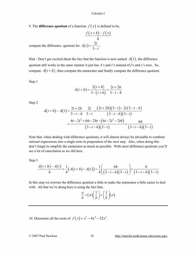
9. The difference quotient of a function ( )f x is defined to be,
( ) ( )f x h f xh
+ −
compute the difference quotient for ( ) 23
tA tt
=−
.
Hint : Don’t get excited about the fact that the function is now named ( )A t , the difference
quotient still works in the same manner it just has A’s and t’s instead of f’s and x’s now. So, compute ( )A t h+ , then compute the numerator and finally compute the difference quotient.
Step 1
( ) ( )( )
2 2 23 3
t h t hA t ht h t h+ +
+ = =− + − −
Step 2
( ) ( ) ( ) ( ) ( )( ) ( )
( )( )( ) ( )( )
2 2
2 2 3 2 32 2 23 3 3 3
6 2 6 2 6 2 2 63 3 3 3
t h t t t ht h tA t h A tt h t t h t
t t h ht t t th ht h t t h t
+ − − − −++ − = − =
− − − − − −
− + − − − −= =
− − − − − −
Note that, when dealing with difference quotients, it will almost always be advisable to combine rational expressions into a single term in preparation of the next step. Also, when doing this don’t forget to simplify the numerator as much as possible. With most difference quotients you’ll see a lot of cancelation as we did here. Step 3
( ) ( ) ( ) ( )( ) ( ) ( ) ( )( )1 1 6 6
3 3 3 3A t h A t hA t h A t
h h h t h t t h t + −
= + − = = − − − − − −
In this step we rewrote the difference quotient a little to make the numerator a little easier to deal with. All that we’re doing here is using the fact that,
( ) ( )1 1a a ab b b
= =
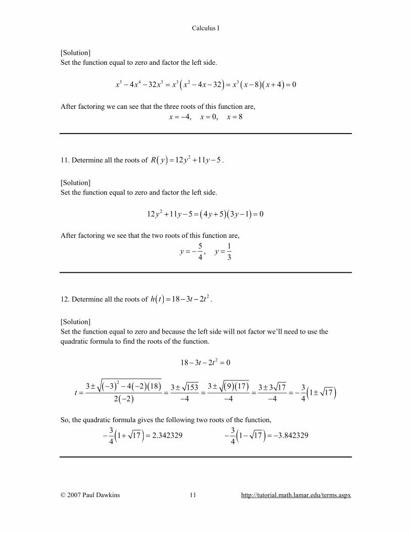
10. Determine all the roots of ( ) 5 4 34 32f x x x x= − − .
Calculus I
© 2007 Paul Dawkins 11 http://tutorial.math.lamar.edu/terms.aspx
[Solution] Set the function equal to zero and factor the left side.
( ) ( )( )5 4 3 3 2 34 32 4 32 8 4 0x x x x x x x x x− − = − − = − + = After factoring we can see that the three roots of this function are, 4, 0, 8x x x= − = = 11. Determine all the roots of ( ) 212 11 5R y y y= + − .
[Solution] Set the function equal to zero and factor the left side. ( ) ( )212 11 5 4 5 3 1 0y y y y+ − = + − = After factoring we see that the two roots of this function are,
5 1,4 3
y y= − =
12. Determine all the roots of ( ) 218 3 2h t t t= − − .
[Solution] Set the function equal to zero and because the left side will not factor we’ll need to use the quadratic formula to find the roots of the function. 218 3 2 0t t− − =
( ) ( ) ( )
( )( ) ( ) ( )
23 3 4 2 18 3 9 173 153 3 3 17 3 1 172 2 4 4 4 4
t± − − − ±± ±
= = = = = − ±− − − −
So, the quadratic formula gives the following two roots of the function,
( ) ( )3 31 17 2.342329 1 17 3.8423294 4
− + = − − = −
Calculus I
© 2007 Paul Dawkins 12 http://tutorial.math.lamar.edu/terms.aspx
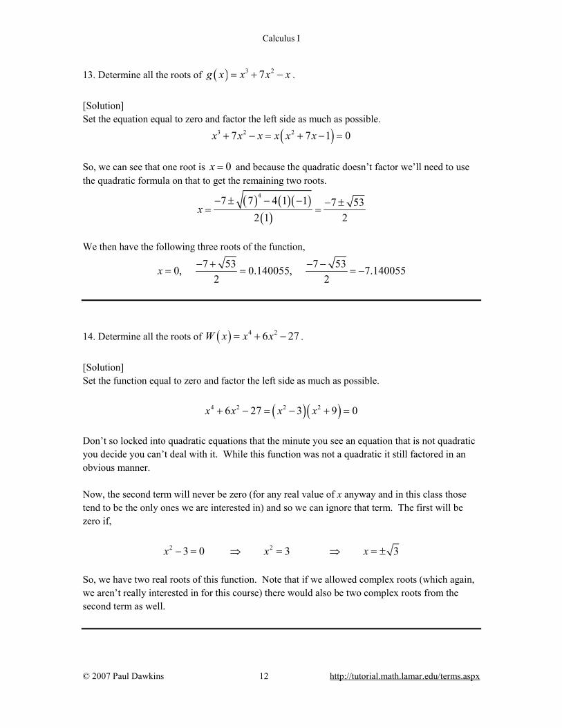
13. Determine all the roots of ( ) 3 27g x x x x= + − .
[Solution] Set the equation equal to zero and factor the left side as much as possible.
( )3 2 27 7 1 0x x x x x x+ − = + − = So, we can see that one root is 0x = and because the quadratic doesn’t factor we’ll need to use the quadratic formula on that to get the remaining two roots.
( ) ( )( )
( )
47 7 4 1 1 7 532 1 2
x− ± − − − ±
= =
We then have the following three roots of the function,
7 53 7 530, 0.140055, 7.1400552 2
x − + − −= = = −
14. Determine all the roots of ( ) 4 26 27W x x x= + − .
[Solution] Set the function equal to zero and factor the left side as much as possible.
( )( )4 2 2 26 27 3 9 0x x x x+ − = − + = Don’t so locked into quadratic equations that the minute you see an equation that is not quadratic you decide you can’t deal with it. While this function was not a quadratic it still factored in an obvious manner. Now, the second term will never be zero (for any real value of x anyway and in this class those tend to be the only ones we are interested in) and so we can ignore that term. The first will be zero if,
2 23 0 3 3x x x− = ⇒ = ⇒ = ± So, we have two real roots of this function. Note that if we allowed complex roots (which again, we aren’t really interested in for this course) there would also be two complex roots from the second term as well.
Calculus I
© 2007 Paul Dawkins 13 http://tutorial.math.lamar.edu/terms.aspx
15. Determine all the roots of ( )5 43 37 8f t t t t= − − .
[Solution] Set the function equal to zero and factor the left side as much as possible.
5 4 2 1 1 13 3 3 3 3 37 8 7 8 8 1 0t t t t t t t t t
− − = − − = − + =
Don’t so locked into quadratic equations that the minute you see an equation that is not quadratic you decide you can’t deal with it. While this function was not a quadratic it still factored, it just wasn’t as obvious that it did in this case. You could have clearly seen that if factored if it had been,
( )2 7 8t t t− − but notice that the only real difference is that the exponents are fractions now, but it still has the same basic form and so can be factored. Okay, back to the problem. From the factored form we get,
( )
1 133 3
1 133 3
0
8 0 8 8 512
1 0 1 1 1
t
t t t
t t t
=
− = ⇒ = ⇒ = =
+ = ⇒ = − ⇒ = − = −
So, the function has three roots, 1, 0, 512t t t= − = =
16. Determine all the roots of ( ) 45 8
zh zz z
= −− −
.
[Solution] Set the function equal to zero and clear the denominator by multiplying by the least common denominator, ( )( )5 8z z− − , and then solve the resulting equation.
Calculus I
© 2007 Paul Dawkins 14 http://tutorial.math.lamar.edu/terms.aspx
( )( )
( ) ( )
( )( )
2
45 8 05 8
8 4 5 0
12 20 010 2 0
zz zz z
z z z
z zz z
− − − = − − − − − =
− + =
− − =
So, it looks like the function has two roots, 2z = and 10z = however recall that because we started off with a function that contained rational expressions we need to go back to the original function and make sure that neither of these will create a division by zero problem in the original function. In this case neither do and so the two roots are, 2 10z z= =
17. Determine all the roots of ( ) 2 41 2 3
w wg ww w
−= +
+ −.
[Solution] Set the function equal to zero and clear the denominator by multiplying by the least common denominator, ( ) ( )1 2 3w w+ − , and then solve the resulting equation.
( ) ( )
( ) ( )( )2
2 41 2 3 01 2 3
2 2 3 4 1 0
5 9 4 0
w ww ww w
w w w w
w w
− + − + = + − − + − + =
− − =
This quadratic doesn’t factor so we’ll need to use the quadratic formula to get the solution.
( ) ( ) ( )
( )
29 9 4 5 4 9 1612 5 10
w± − − − ±
= =
So, it looks like this function has the following two roots,
9 161 9 1612.168858 0.36885810 10
+ −= = −
Recall that because we started off with a function that contained rational expressions we need to go back to the original function and make sure that neither of these will create a division by zero problem in the original function. Neither of these do and so they are the two roots of this function.

Calculus I
© 2007 Paul Dawkins 15 http://tutorial.math.lamar.edu/terms.aspx
18. Find the domain and range of ( ) 23 2 1Y t t t= − + .
[Solution] This is a polynomial (a 2nd degree polynomial in fact) and so we know that we can plug any value of t into the function and so the domain is all real numbers or, ( )Domain : or ,t− ∞ < < ∞ −∞ ∞ The graph of this 2nd degree polynomial (or quadratic) is a parabola that opens upwards (because the coefficient of the 2t is positive) and so we know that the vertex will be the lowest point on the graph. This also means that the function will take on all values greater than or equal to the y-coordinate of the vertex which will in turn give us the range. So, we need the vertex of the parabola. The t-coordinate is,
( )2 1
2 3 3t −
= − =
and the y coordinate is then, 1 23 3
Y =
.
The range is then,
2Range : ,3
∞
19. Find the domain and range of ( ) 2 4 7g z z z= − − + .
[Solution] This is a polynomial (a 2nd degree polynomial in fact) and so we know that we can plug any value of z into the function and so the domain is all real numbers or, ( )Domain : or ,z− ∞ < < ∞ −∞ ∞ The graph of this 2nd degree polynomial (or quadratic) is a parabola that opens downwards (because the coefficient of the 2z is negative) and so we know that the vertex will be the highest

Calculus I
© 2007 Paul Dawkins 16 http://tutorial.math.lamar.edu/terms.aspx
point on the graph. This also means that the function will take on all values less than or equal to the y-coordinate of the vertex which will in turn give us the range. So, we need the vertex of the parabola. The z-coordinate is,
( )
4 22 1
z −= − = −
−
and the y coordinate is then, ( )2 11g − = .
The range is then, ( ]Range : ,11−∞
20. Find the domain and range of ( ) 22 1f z z= + + .
[Solution] We know that when we have square roots that we can’t take the square root of a negative number. However, because, 2 1 1z + ≥ we will never be taking the square root of a negative number in this case and so the domain is all real numbers or, ( )Domain : or ,z− ∞ < < ∞ −∞ ∞ For the range we need to recall that square roots will only return values that are positive or zero and in fact the only way we can get zero out of a square root will be if we take the square root of zero. For our function, as we’ve already noted, the quantity that is under the root is always at least 1 and so this root will never be zero. Also recall that we have the following fact about square roots,
If 1 then 1x x≥ ≥ So, we now know that,
2 1 1z + ≥ Finally, we are adding 2 onto the root and so we know that the function must always be greater than or equal to 3 and so the range is, [ )Range : 3,∞

Calculus I
© 2007 Paul Dawkins 17 http://tutorial.math.lamar.edu/terms.aspx
21. Find the domain and range of ( ) 3 14 3h y y= − + .
[Solution] In this case we need to require that,
1414 3 03
y y+ ≥ ⇒ ≥ −
in order to make sure that we don’t take the square root of negative numbers. The domain is then,
14 14Domain : or ,3 3
y − ≤ < ∞ − ∞
For the range for this function we can notice that the quantity under the root can be zero (if
143y = − ). Also note that because the quantity under the root is a line it will take on all positive
values and so the square root will in turn take on all positive value and zero. The square root is then multiplied by -3. This won’t change the fact that the root can be zero, but the minus sign will change the sign of the non-zero values from positive to negative. The 3 will only affect the general size of the square root but it won’t change the fact that the square root will still take on all positive (or negative after we add in the minus sign) values. The range is then, ( ]Range : ,0∞ 22. Find the domain and range of ( ) 5 8M x x= − + .
[Solution] We’re dealing with an absolute value here and the quantity inside is a line, which we can plug all values of x into, and so the domain is all real numbers or, ( )Domain : or ,x− ∞ < < ∞ −∞ ∞ For the range let’s again note that the quantity inside the absolute value is a linear function that will take on all real values. We also know that absolute value functions will never be negative and will only be zero if we take the absolute value of zero. So we now know that, 8 0x + ≥
Calculus I
© 2007 Paul Dawkins 18 http://tutorial.math.lamar.edu/terms.aspx
However, we are subtracting this from 5 and so we’ll be subtracting a positive or zero number from 5 and so the range is, ( ]Range : ,5−∞
23. Find the domain of ( )3 3 112 7
w wf ww
− +=
−.
[Solution] In this case we need to avoid division by zero issues and so we’ll need to determine where the denominator is zero. To do this we will solve,
712 7 012
w w− = ⇒ =
We can plug all other values of w into the function without any problems and so the domain is,
7Domain : All real numbers except 12
w =
24. Find the domain of ( ) 3 2
510 9
R zz z z
=+ +
.
[Solution] In this case we need to avoid division by zero issues and so we’ll need to determine where the denominator is zero. To do this we will solve,
( ) ( )( )3 2 210 9 10 9 1 9 0 0, 1, 9z z z z z z z z z z z z+ + = + + = + + = ⇒ = = − = − The three values above are the only values of z that we can’t plug into the function. All other values of z can be plugged into the function and will return real values. The domain is then, Domain : All real numbers except 0, 1, 9z z z= = − = −
25. Find the domain of ( )3
2
67 4
t tg tt t−
=− −
.
Calculus I
© 2007 Paul Dawkins 19 http://tutorial.math.lamar.edu/terms.aspx
[Solution] In this case we need to avoid division by zero issues and so we’ll need to determine where the denominator is zero. To do this we will solve,
( ) ( )( )
( ) ( )2
2 1 1 4 4 7 17 4 0 1 1132 4 8
t t t± − − −
− − = ⇒ = = − ±−
The two values above are the only values of t that we can’t plug into the function. All other values of t can be plugged into the function and will return real values. The domain is then,
( )1Domain : All real numbers except 1 1138
t = − ±
26. Find the domain of ( ) 225g x x= − .
[Solution] In this case we need to avoid square roots of negative numbers and so we need to require, 225 0x− ≥ Note that once we have the original inequality written down we can do a little rewriting of things as follows to make things a little easier to see. 2 25 5 5x x≤ ⇒ − ≤ ≤ At this point it should be pretty easy to find the values of x that will keep the quantity under the radical positive or zero and so we won’t need to do a numberline or sign table to determine the range. The domain is then, Domain : 5 5x− ≤ ≤
27. Find the domain of ( ) 4 3 220h x x x x= − − .

Calculus I
© 2007 Paul Dawkins 20 http://tutorial.math.lamar.edu/terms.aspx
Step 1 Hint : We need to avoid negative numbers under the square root and because the quantity under the root is a polynomial we know that it can only change sign if it goes through zero and so we first need to determine where it is zero. [Show Step One] In this case we need to avoid square roots of negative numbers and so we need to require,
( ) ( )( )4 3 2 2 2 220 20 5 4 0x x x x x x x x x− − = − − = − + ≥ Once we have the polynomial in factored form we can see that the left side will be zero at 0x = ,
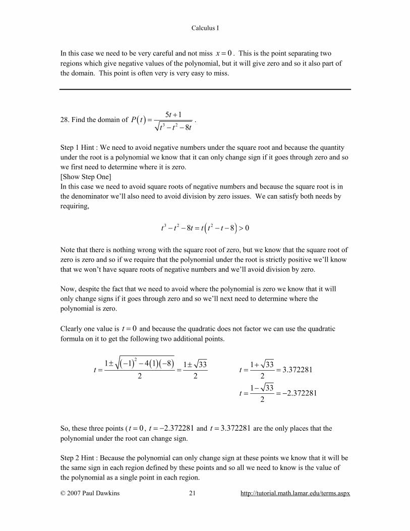
4x = − and 5x = . Because the quantity under the radical is a polynomial we know that it can only change sign if it goes through zero and so these are the only points the only places where the polynomial on the left can change sign. Step 2 Hint : Because the polynomial can only change sign at these points we know that it will be the same sign in each region defined by these points and so all we need to know is the value of the polynomial as a single point in each region. [Show Step Two] Here is a number line giving the value/sign of the polynomial at a test point in each of the region defined by these three points. To make it a little easier to read the number line let’s define the polynomial under the radical to be, ( ) ( ) ( )4 3 2 220 5 4R x x x x x x x= − − = − + Now, here is the number line,
Step 3 Hint : Now all we need to do is write down the values of x where the polynomial under the root will be positive or zero and we’ll have the domain. Be careful with the points where the polynomial is zero. [Show Step Three] The domain will then be all the points where the polynomial under the root is positive or zero and so the domain is, Domain : 4, 0, 5x x x− ∞ < ≤ − = ≤ < ∞
Calculus I
© 2007 Paul Dawkins 21 http://tutorial.math.lamar.edu/terms.aspx
In this case we need to be very careful and not miss 0x = . This is the point separating two regions which give negative values of the polynomial, but it will give zero and so it also part of the domain. This point is often very is very easy to miss.
28. Find the domain of ( )3 2
5 18
tP tt t t
+=
− −.
Step 1 Hint : We need to avoid negative numbers under the square root and because the quantity under the root is a polynomial we know that it can only change sign if it goes through zero and so we first need to determine where it is zero. [Show Step One] In this case we need to avoid square roots of negative numbers and because the square root is in the denominator we’ll also need to avoid division by zero issues. We can satisfy both needs by requiring,
( )3 2 28 8 0t t t t t t− − = − − > Note that there is nothing wrong with the square root of zero, but we know that the square root of zero is zero and so if we require that the polynomial under the root is strictly positive we’ll know that we won’t have square roots of negative numbers and we’ll avoid division by zero. Now, despite the fact that we need to avoid where the polynomial is zero we know that it will only change signs if it goes through zero and so we’ll next need to determine where the polynomial is zero. Clearly one value is 0t = and because the quadratic does not factor we can use the quadratic formula on it to get the following two additional points.
( ) ( ) ( )21 1 4 1 8 1 33 1 33 3.3722812 2 2
1 33 2.3722812
t t
t
± − − − ± += = = =
−= = −
So, these three points ( 0t = , 2.372281t = − and 3.372281t = are the only places that the polynomial under the root can change sign. Step 2 Hint : Because the polynomial can only change sign at these points we know that it will be the same sign in each region defined by these points and so all we need to know is the value of the polynomial as a single point in each region.
Calculus I
© 2007 Paul Dawkins 22 http://tutorial.math.lamar.edu/terms.aspx
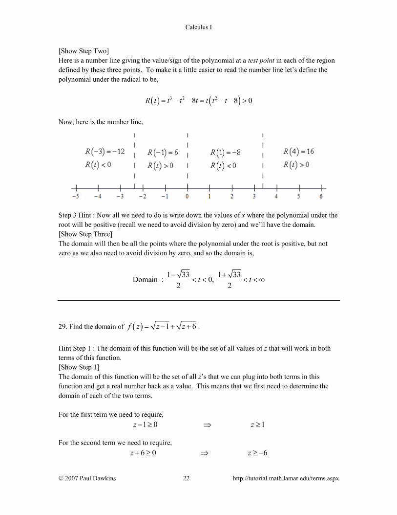
[Show Step Two] Here is a number line giving the value/sign of the polynomial at a test point in each of the region defined by these three points. To make it a little easier to read the number line let’s define the polynomial under the radical to be,
( ) ( )3 2 28 8 0R t t t t t t t= − − = − − > Now, here is the number line,
Step 3 Hint : Now all we need to do is write down the values of x where the polynomial under the root will be positive (recall we need to avoid division by zero) and we’ll have the domain. [Show Step Three] The domain will then be all the points where the polynomial under the root is positive, but not zero as we also need to avoid division by zero, and so the domain is,
1 33 1 33Domain : 0,2 2
t t− +< < < < ∞
29. Find the domain of ( ) 1 6f z z z= − + + .
Hint Step 1 : The domain of this function will be the set of all values of z that will work in both terms of this function. [Show Step 1] The domain of this function will be the set of all z’s that we can plug into both terms in this function and get a real number back as a value. This means that we first need to determine the domain of each of the two terms. For the first term we need to require, 1 0 1z z− ≥ ⇒ ≥ For the second term we need to require, 6 0 6z z+ ≥ ⇒ ≥ −
Calculus I
© 2007 Paul Dawkins 23 http://tutorial.math.lamar.edu/terms.aspx
Hint Step 2 : What values of z are in both of these? [Show Step 2] Now, we just need the set of z’s that are in both conditions above. In this case notice that all the z that satisfy 1z ≥ will also satisfy 6z ≥ − . The reverse is not true however. Any z that is in the range 6 1z− ≤ < will satisfy 6z ≥ but will not satisfy 1z ≥ . So, in this case, the domain is in fact just the first condition above or, Domain : 1z ≥
30. Find the domain of ( ) 12 92
h y yy
= + −−
.
Hint Step 1 : The domain of this function will be the set of all values of y that will work in both terms of this function. [Show Step 1] The domain of this function will be the set of all y’s that we can plug into both terms in this function and get a real number back as a value. This means that we first need to determine the domain of each of the two terms. For the first term we need to require,
92 9 02
y y+ ≥ ⇒ ≥ −
For the second term we need to require, 2 0 2y y− > ⇒ < Note that we need the second condition to be strictly positive to avoid division by zero as well. Hint Step 2 : What values of y are in both of these? [Show Step 2] Now, we just need the set of y’s that are in both conditions above. In this case we need all the y’s that will be greater than or equal to 9
2− AND less than 2. The domain is then,
9Domain : 22
y− ≤ <
Calculus I
© 2007 Paul Dawkins 24 http://tutorial.math.lamar.edu/terms.aspx
31. Find the domain of ( ) 24 369
A x xx
= − −−
.
Hint Step 1 : The domain of this function will be the set of all values of x that will work in both terms of this function. [Show Step 1] The domain of this function will be the set of all x’s that we can plug into both terms in this function and get a real number back as a value. This means that we first need to determine the domain of each of the two terms. For the first term we need to require, 9 0 9x x− ≠ ⇒ ≠ For the second term we need to require, 2 236 0 36 6 & 6x x x x− ≥ → ≥ ⇒ ≤ − ≥ Hint Step 2 : What values of x are in both of these? [Show Step 2] Now, we just need the set of x’s that are in both conditions above. In this case the second condition gives us most of the domain as it is the most restrictive. The first term is okay as long as we avoid 9x = and because this point will in fact satisfy the second condition we’ll need to make sure and exclude it. The domain is then, Domain : 6 & 6, 9x x x≤ − ≥ ≠
32. Find the domain of ( ) 2 31 1Q y y y= + − − .
[Solution] The domain of this function will be the set of y’s that will work in both terms of this function. So, we need the domain of each of the terms. For the first term let’s note that, 2 1 1y + ≥ and so will always be positive. The domain of the first term is then all real numbers. For the second term we need to notice that we’re dealing with the cube root in this case and we can plug all real numbers into a cube root and so the domain of this term is again all real numbers.
Calculus I
© 2007 Paul Dawkins 25 http://tutorial.math.lamar.edu/terms.aspx
So, the domain of both terms is all real numbers and so the domain of the function as a whole must also be all real numbers or, Domain : y− ∞ < < ∞
33. Compute ( )( )f g xo and ( )( )g f xo for ( ) 4 1f x x= − , ( ) 6 7g x x= + .
[Solution] Not much to do here other than to compute each of these.
( )( ) ( )
( ) ( ) ( ) [ ] ( )
6 7 4 6 7 1
4 1 6 7 4 1 28 1
f g x f g x f x x
g f x g f x g x x x
= = + = + −
= = − = + − = −
o
o
34. Compute ( )( )f g xo and ( )( )g f xo for ( ) 5 2f x x= + , ( ) 2 14g x x x= − .
[Solution] Not much to do here other than to compute each of these.
( ) ( ) ( ) ( )
( ) ( ) ( ) [ ] ( ) ( )
2 2 2
2 2
14 5 14 2 5 70 2
5 2 5 2 14 5 2 25 50 24
f g x f g x f x x x x x x
g f x g f x g x x x x x
= = − = − + = − +
= = + = + − + = − −
o
o
35. Compute ( )( )f g xo and ( )( )g f xo for ( ) 2 2 1f x x x= − + , ( ) 28 3g x x= − .
[Solution] Not much to do here other than to compute each of these.
Calculus I
© 2007 Paul Dawkins 26 http://tutorial.math.lamar.edu/terms.aspx
( )( ) ( ) ( ) ( )
( )( ) ( )
( )
22 2 2 4 2
2
22 4 3 2
8 3 8 3 2 8 3 1 9 42 49
2 1
8 3 2 1 3 12 18 12 5
f g x f g x f x x x x x
g f x g f x g x x
x x x x x x
= = − = − − − + = − +
= = − +
= − − + = − + − + +
o
o
36. Compute ( )( )f g xo and ( )( )g f xo for ( ) 2 3f x x= + , ( ) 25g x x= + .
[Solution] Not much to do here other than to compute each of these.
( )( ) ( ) ( )
( )( ) ( ) ( )
22 2 2
22 2 4 2
5 5 3 8
3 5 3 6 14
f g x f g x f x x x
g f x g f x g x x x x
= = − = + + = +
= = + = + + = + +
o
o
Review : Inverse Functions 1. Find the inverse for ( ) 6 15f x x= + . Verify your inverse by computing one or both of the
composition as discussed in this section. Hint : Remember the process described in this section. Replace the ( )f x , interchange the x’s
and y’s, solve for y and the finally replace the y with ( )1f x− .
Step 1 6 15y x= + Step 2 6 15x y= + Step 3

Calculus I
© 2007 Paul Dawkins 27 http://tutorial.math.lamar.edu/terms.aspx
( ) ( ) ( )1
15 6
1 115 156 6
x y
y x f x x−
− =
= − → = −
Finally, compute either ( )( )1f f x−o or ( )( )1f f x− o to verify our work.
Step 4
Either composition can be done so let’s do ( )( )1f f x−o in this case.
( )( ) ( )
( )
1 1
16 15 15615 15
f f x f f x
x
xx
− − = = − +
= − +=
o
So, we got x out of the composition and so we know we’ve done our work correctly. 2. Find the inverse for ( ) 3 29h x x= − . Verify your inverse by computing one or both of the
composition as discussed in this section. Hint : Remember the process described in this section. Replace the ( )h x , interchange the x’s
and y’s, solve for y and the finally replace the y with ( )1h x− .
Step 1 3 29y x= − Step 2 3 29x y= − Step 3
( ) ( ) ( )1
3 29
1 13 329 29
x y
y x h x x−
− = −
= − − → = −
Notice that we multiplied the minus sign into the parenthesis. We did this in order to avoid potentially losing the minus sign if it had stayed out in front. This does not need to be done in order to get the inverse.

Calculus I
© 2007 Paul Dawkins 28 http://tutorial.math.lamar.edu/terms.aspx
Finally, compute either ( )( )1h h x−o or ( )( )1h h x− o to verify our work.
Step 4
Either composition can be done so let’s do ( )( )1h h x−o in this case.
( )( ) ( )
( )
( )
1 1
13 29 329
3 3
h h x h h x
x
xx
− − = = − −
= − −
=
o
So, we got x out of the composition and so we know we’ve done our work correctly. 3. Find the inverse for ( ) 3 6R x x= + . Verify your inverse by computing one or both of the
composition as discussed in this section. Hint : Remember the process described in this section. Replace the ( )R x , interchange the x’s
and y’s, solve for y and the finally replace the y with ( )1R x− .
Step 1 3 6y x= + Step 2 3 6x y= + Step 3
( )
3
13 3
6
6 6
x y
y x R x x−
− =
= − → = −
Finally, compute either ( )( )1R R x−o or ( )( )1R R x− o to verify our work.
Step 4
Either composition can be done so let’s do ( )( )1R R x− o in this case.

Calculus I
© 2007 Paul Dawkins 29 http://tutorial.math.lamar.edu/terms.aspx
( )( ) ( )
( )
1 1
33
3 3
6 6
R R x R R x
x
xx
− −=
= + −
==
o
So, we got x out of the composition and so we know we’ve done our work correctly.
4. Find the inverse for ( ) ( )54 3 21g x x= − + . Verify your inverse by computing one or both of
the composition as discussed in this section. Hint : Remember the process described in this section. Replace the ( )g x , interchange the x’s
and y’s, solve for y and the finally replace the y with ( )1g x− .
Step 1
( )54 3 21y x= − + Step 2
( )54 3 21x y= − + Step 3
( )
( ) ( )
( )
( ) ( ) ( )
5
5
5
15 5
21 4 31 21 341 21 34
1 13 21 3 214 4
x y
x y
x y
y x g x x−
− = −
− = −
− = −
= + − → = + −
Finally, compute either ( )( )1g g x−o or ( )( )1g g x− o to verify our work.
Step 4
Either composition can be done so let’s do ( )( )1g g x−o in this case.

Calculus I
© 2007 Paul Dawkins 30 http://tutorial.math.lamar.edu/terms.aspx
( )( ) ( )
( )
( )
( )
( )
1 1
5
5
5
5
14 3 21 3 214
14 21 214
14 21 214
21 21
g g x g g x
x
x
x
xx
− − =
= + − − +
= − +
= − +
= − +
=
o
So, we got x out of the composition and so we know we’ve done our work correctly.
5. Find the inverse for ( ) 5 9 11W x x= − . Verify your inverse by computing one or both of the
composition as discussed in this section. Hint : Remember the process described in this section. Replace the ( )W x , interchange the x’s
and y’s, solve for y and the finally replace the y with ( )1W x− .
Step 1
5 9 11y x= − Step 2
5 9 11x y= − Step 3
( ) ( ) ( )
5
5
5
5 1 5
9 11
9 119 11
1 19 911 11
x y
x yx y
y x W x x−
= −
= −
− = −
= − − → = −
Notice that we multiplied the minus sign into the parenthesis. We did this in order to avoid potentially losing the minus sign if it had stayed out in front. This does not need to be done in order to get the inverse.
Finally, compute either ( )( )1W W x−o or ( )( )1W W x− o to verify our work.

Calculus I
© 2007 Paul Dawkins 31 http://tutorial.math.lamar.edu/terms.aspx
Step 4
Either composition can be done so let’s do ( )( )1W W x− o in this case.
( )( ) ( )
( )[ ]( )
( )
1 1
551 9 9 11
111 9 9 11111 1111
W W x W W x
x
x
x
x
− −=
= − −
= − −
=
=
o
So, we got x out of the composition and so we know we’ve done our work correctly.
6. Find the inverse for ( ) 7 5 8f x x= + . Verify your inverse by computing one or both of the
composition as discussed in this section. Hint : Remember the process described in this section. Replace the ( )f x , interchange the x’s
and y’s, solve for y and the finally replace the y with ( )1f x− .
Step 1
7 5 8y x= + Step 2
7 5 8x y= + Step 3
( ) ( ) ( )
7
7
7
7 1 7
5 8
5 88 5
1 18 85 5
x y
x yx y
y x f x x−
= +
= +
− =
= − → = −
Finally, compute either ( )( )1f f x−o or ( )( )1f f x− o to verify our work.
Step 4
Calculus I
© 2007 Paul Dawkins 32 http://tutorial.math.lamar.edu/terms.aspx
Either composition can be done so let’s do ( )( )1f f x−o in this case.
( )( ) ( )
( )
1 1
77
77
7 7
15 8 85
8 8
f f x f f x
x
x
xx
− − =
= − +
= − +
==
o
So, we got x out of the composition and so we know we’ve done our work correctly.
7. Find the inverse for ( ) 1 94
xh xx
+=
−. Verify your inverse by computing one or both of the
composition as discussed in this section. Hint : Remember the process described in this section. Replace the ( )h x , interchange the x’s
and y’s, solve for y and the finally replace the y with ( )1h x− .
Step 1
1 94
xyx
+=
−
Step 2
1 94
yxy
+=
−
Step 3
( )
( )
( )1
1 94
4 1 94 1 9
4 1 94 1 9
4 1 4 19 9
yxy
x y yx xy y
x y xyx x y
x xy h xx x
−
+=
−
− = +
− = +− = +
− = +
− −= → =
+ +

Calculus I
© 2007 Paul Dawkins 33 http://tutorial.math.lamar.edu/terms.aspx
Note that the Algebra in these kinds of problems can often be fairly messy, but don’t let that make you decide that you can’t do these problems. Messy Algebra will be a fairly common occurrence in a Calculus class so you’ll need to get used to it!
Finally, compute either ( )( )1h h x−o or ( )( )1h h x− o to verify our work.
Step 4
Either composition can be done so let’s do ( )( )1h h x− o in this case. As with the previous step,
the Algebra here is going to be messy and in fact will probably be messier.
( )( ) ( )
( ) ( )( )
1 1
1 94 144
1 9 494
4 1 9 49 4 1 94 36 436 9 1 93737
h h x h h x
xxx
x xx
x xx xx xx x
x
x
− −= + − −− =
+ − + − + − −
=− + +
+ − +=
− + +
=
=
o
In order to do the simplification we multiplied the numerator and denominator of the initial fraction by 4 x− in order to clear out some of the denominators. This in turn allowed a fair amount of simplification. So, we got x out of the composition and so we know we’ve done our work correctly.
8. Find the inverse for ( ) 6 108 7
xf xx−
=+
. Verify your inverse by computing one or both of the
composition as discussed in this section. Hint : Remember the process described in this section. Replace the ( )f x , interchange the x’s
and y’s, solve for y and the finally replace the y with ( )1f x− .
Step 1
6 108 7
xyx−
=+

Calculus I
© 2007 Paul Dawkins 34 http://tutorial.math.lamar.edu/terms.aspx
Step 2
6 108 7
yxy−
=+
Step 3
( )
( )
( )1
6 108 7
8 7 6 108 7 6 10
8 10 6 78 10 6 7
6 7 6 78 10 8 10
yxy
x y yxy x y
xy y xx y x
x xy f xx x
−
−=
+
+ = −
+ = −+ = −
+ = −
− −= → =
+ +
Note that the Algebra in these kinds of problems can often be fairly messy, but don’t let that make you decide that you can’t do these problems. Messy Algebra will be a fairly common occurrence in a Calculus class so you’ll need to get used to it!
Finally, compute either ( )( )1f f x−o or ( )( )1f f x− o to verify our work.
Step 4
Either composition can be done so let’s do ( )( )1f f x−o in this case. As with the previous step,
the Algebra here is going to be messy and in fact will probably be messier.
( )( ) ( )
( ) ( )( ) ( )
1 1
6 76 108 108 10
6 7 8 108 78 10
6 8 10 10 6 78 6 7 7 8 1048 60 60 7048 56 56 70118118
f f x f f x
xxx
x xx
x xx x
x xx x
x
x
− − = − − ++ =
− + + + + − −
=− + +
+ − +=
− + +
=
=
o
So, we got x out of the composition and so we know we’ve done our work correctly.
Calculus I
© 2007 Paul Dawkins 35 http://tutorial.math.lamar.edu/terms.aspx
Review : Trig Functions
1. Determine the exact value of 5cos6π
without using a calculator.
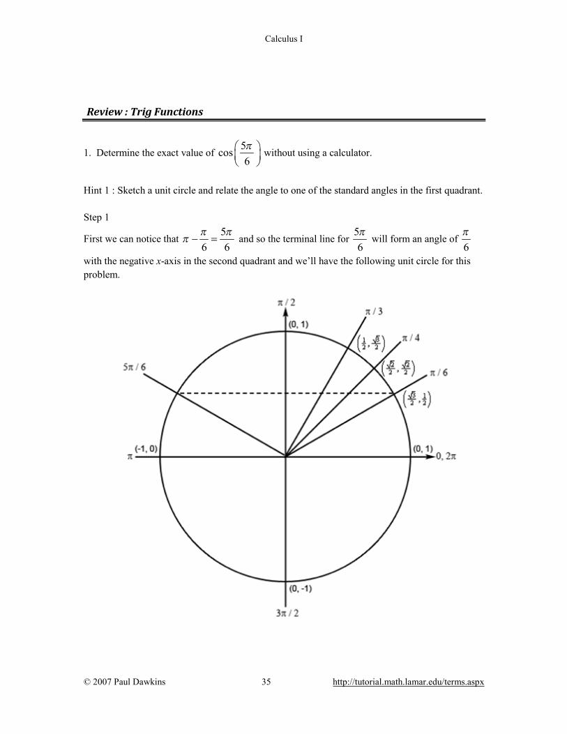
Hint 1 : Sketch a unit circle and relate the angle to one of the standard angles in the first quadrant. Step 1
First we can notice that 5
6 6π π
π − = and so the terminal line for 56π
will form an angle of 6π
with the negative x-axis in the second quadrant and we’ll have the following unit circle for this problem.
Calculus I
© 2007 Paul Dawkins 36 http://tutorial.math.lamar.edu/terms.aspx
Hint 2 : Given the obvious symmetry in the unit circle relate the coordinates of the line
representing 56π
to the coordinates of the line representing 6π
and use those to answer the
question. Step 2
The coordinates of the line representing 56π
will be the same as the coordinates of the line
representing 6π
except that the x coordinate will now be negative. So, our new coordinates will
then be 3 1,
2 2
−
and so the answer is,
5 3cos6 2π = −
2. Determine the exact value of 4sin3π −
without using a calculator.
Hint 1 : Sketch a unit circle and relate the angle to one of the standard angles in the first quadrant. Step 1
First we can notice that 4
3 3π π
π− − = − and so (remembering that negative angles are rotated
clockwise) we can see that the terminal line for 43π
− will form an angle of 3π
with the negative
x-axis in the second quadrant and we’ll have the following unit circle for this problem.

Calculus I
© 2007 Paul Dawkins 37 http://tutorial.math.lamar.edu/terms.aspx
Hint 2 : Given the obvious symmetry in the unit circle relate the coordinates of the line
representing 43π
− to the coordinates of the line representing 3π
and use those to answer the
question. Step 2
The coordinates of the line representing 43π
− will be the same as the coordinates of the line
representing 3π
except that the x coordinate will now be negative. So, our new coordinates will
then be 1 3,2 2
−
and so the answer is,
4 3sin3 2π − =

Calculus I
© 2007 Paul Dawkins 38 http://tutorial.math.lamar.edu/terms.aspx
3. Determine the exact value of 7sin4π
without using a calculator.
Hint 1 : Sketch a unit circle and relate the angle to one of the standard angles in the first quadrant. Step 1
First we can notice that 72
4 4π π
π − = and so the terminal line for 74π
will form an angle of 4π
with the positive x-axis in the fourth quadrant and we’ll have the following unit circle for this problem.
Hint 2 : Given the obvious symmetry in the unit circle relate the coordinates of the line
representing 74π
to the coordinates of the line representing 4π
and use those to answer the
question.
Calculus I
© 2007 Paul Dawkins 39 http://tutorial.math.lamar.edu/terms.aspx
Step 2
The coordinates of the line representing 74π
will be the same as the coordinates of the line
representing 4π
except that the y coordinate will now be negative. So, our new coordinates will
then be 2 2,
2 2
−
and so the answer is,
7 2sin4 2π = −
4. Determine the exact value of 2cos3π −
without using a calculator.
Hint 1 : Sketch a unit circle and relate the angle to one of the standard angles in the first quadrant. Step 1
First we can notice that 2
3 3π π
π− + = − so (recalling that negative angles rotate clockwise and
positive angles rotation counter clockwise) the terminal line for 23π
− will form an angle of 3π
with the negative x-axis in the third quadrant and we’ll have the following unit circle for this problem.

Calculus I
© 2007 Paul Dawkins 40 http://tutorial.math.lamar.edu/terms.aspx
Hint 2 : Given the obvious symmetry in the unit circle relate the coordinates of the line
representing 23π
− to the coordinates of the line representing 3π
and use those to answer the
question. Step 2
The line representing 23π
− is a mirror image of the line representing 3π
and so the coordinates
for 23π
− will be the same as the coordinates for 3π
except that both coordinates will now be
negative. So, our new coordinates will then be 1 3,2 2
− −
and so the answer is,
2 1cos3 2π − = −
Calculus I
© 2007 Paul Dawkins 41 http://tutorial.math.lamar.edu/terms.aspx
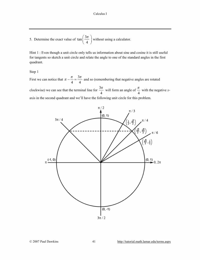
5. Determine the exact value of 3tan4π
without using a calculator.
Hint 1 : Even though a unit circle only tells us information about sine and cosine it is still useful for tangents so sketch a unit circle and relate the angle to one of the standard angles in the first quadrant. Step 1
First we can notice that 3
4 4π π
π − = and so (remembering that negative angles are rotated
clockwise) we can see that the terminal line for 34π
will form an angle of 4π
with the negative x-
axis in the second quadrant and we’ll have the following unit circle for this problem.
Calculus I
© 2007 Paul Dawkins 42 http://tutorial.math.lamar.edu/terms.aspx
Hint 2 : Given the obvious symmetry in the unit circle relate the coordinates of the line
representing 34π
to the coordinates of the line representing 4π
and and then recall how tangent is
defined in terms of sine and cosine to answer the question. Step 2
The coordinates of the line representing 34π
will be the same as the coordinates of the line
representing 4π
except that the x coordinate will now be negative. So, our new coordinates will
then be 2 2,
2 2
−
and so the answer is,
3sin 23 4 2tan 134 2cos 24
ππ
π
= = = − −
6. Determine the exact value of 11sec
6π −
without using a calculator.
Hint 1 : Even though a unit circle only tells us information about sine and cosine it is still useful for secant so sketch a unit circle and relate the angle to one of the standard angles in the first quadrant. Step 1
First we can notice that 112
6 6π π
π− = − and so (remembering that negative angles are rotated
clockwise) we can see that the terminal line for 11
6π
− will form an angle of 6π
with the positive
x-axis in the first quadrant. In other words 11
6π
− and 6π
represent the same angle. So, we’ll
have the following unit circle for this problem.
Calculus I
© 2007 Paul Dawkins 43 http://tutorial.math.lamar.edu/terms.aspx
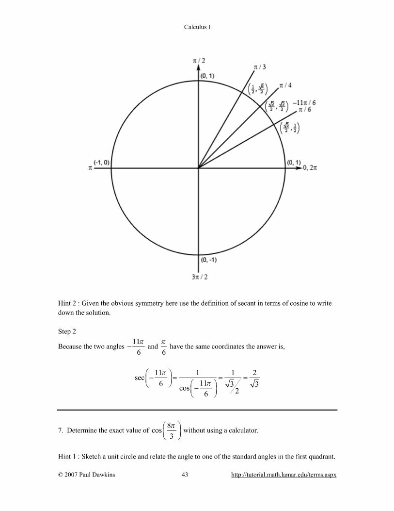
Hint 2 : Given the obvious symmetry here use the definition of secant in terms of cosine to write down the solution. Step 2
Because the two angles 11
6π
− and 6π
have the same coordinates the answer is,
11 1 1 2sec116 3 3cos 26
ππ
− = = = −
7. Determine the exact value of 8cos3π
without using a calculator.
Hint 1 : Sketch a unit circle and relate the angle to one of the standard angles in the first quadrant.

Calculus I
© 2007 Paul Dawkins 44 http://tutorial.math.lamar.edu/terms.aspx
Step 1
First we can notice that 2 823 3π π
π + = and because 2π is one complete revolution the angles
83π
and 23π
are the same angle. Also, note that 2
3 3π π
π − = and so the terminal line for 83π
will form an angle of 3π
with the negative x-axis in the second quadrant and we’ll have the
following unit circle for this problem.
Hint 2 : Given the obvious symmetry in the unit circle relate the coordinates of the line
representing 83π
to the coordinates of the line representing 23π
and use those to answer the
question. Step 2
Calculus I
© 2007 Paul Dawkins 45 http://tutorial.math.lamar.edu/terms.aspx
The coordinates of the line representing 83π
will be the same as the coordinates of the line
representing 3π
except that the x coordinate will now be negative. So, our new coordinates will
then be 1 3,2 2
−
and so the answer is,
8 1cos3 2π = −
8. Determine the exact value of tan3π −
without using a calculator.
Hint 1 : Even though a unit circle only tells us information about sine and cosine it is still useful for tangents so sketch a unit circle and relate the angle to one of the standard angles in the first quadrant. Step 1
To do this problem all we need to notice is that 3π
− will form an angle of 3π
with the positive x-
axis in the fourth quadrant and we’ll have the following unit circle for this problem.
Calculus I
© 2007 Paul Dawkins 46 http://tutorial.math.lamar.edu/terms.aspx
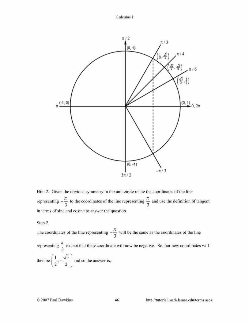
Hint 2 : Given the obvious symmetry in the unit circle relate the coordinates of the line
representing 3π
− to the coordinates of the line representing 3π
and use the definition of tangent
in terms of sine and cosine to answer the question. Step 2
The coordinates of the line representing 3π
− will be the same as the coordinates of the line
representing 3π
except that the y coordinate will now be negative. So, our new coordinates will
then be 1 3,2 2
−
and so the answer is,
Calculus I
© 2007 Paul Dawkins 47 http://tutorial.math.lamar.edu/terms.aspx
sin 3
3 2tan 313 cos 23
ππ
π
− − − = = = − −
9. Determine the exact value of 15tan
4π
without using a calculator.
Hint 1 : Even though a unit circle only tells us information about sine and cosine it is still useful for tangents so sketch a unit circle and relate the angle to one of the standard angles in the first quadrant. Step 1
First we can notice that 154
4 4π π
π − = and also note that 4π is two complete revolutions so the
terminal line for 15
4π
and 4π
− represent the same angle. Also note that 4π
− will form an
angle of 4π
with the positive x-axis in the fourth quadrant and we’ll have the following unit circle
for this problem.

Calculus I
© 2007 Paul Dawkins 48 http://tutorial.math.lamar.edu/terms.aspx
Hint 2 : Given the obvious symmetry in the unit circle relate the coordinates of the line
representing 15
4π
to the coordinates of the line representing 4π
and the definition of tangent in
terms of sine and cosine to answer the question. Step 2
The coordinates of the line representing 15
4π
will be the same as the coordinates of the line
representing 4π
except that the y coordinate will now be negative. So, our new coordinates will
then be 2 2,
2 2
−
and so the answer is,
Calculus I
© 2007 Paul Dawkins 49 http://tutorial.math.lamar.edu/terms.aspx
15sin 215 4 2tan 1154 2cos 24
ππ
π
− = = = −
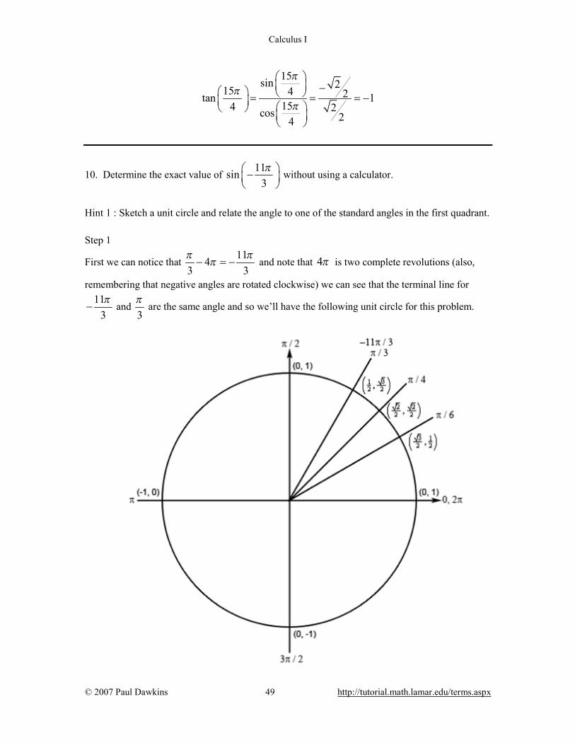
10. Determine the exact value of 11sin
3π −
without using a calculator.
Hint 1 : Sketch a unit circle and relate the angle to one of the standard angles in the first quadrant. Step 1
First we can notice that 114
3 3π π
π− = − and note that 4π is two complete revolutions (also,
remembering that negative angles are rotated clockwise) we can see that the terminal line for 11
3π
− and 3π
are the same angle and so we’ll have the following unit circle for this problem.

Calculus I
© 2007 Paul Dawkins 50 http://tutorial.math.lamar.edu/terms.aspx
Hint 2 : Given the very obvious symmetry here write down the answer to the question. Step 2
Because 11
3π
− and 3π
are the same angle the answer is,
11 3sin3 2π − =
11. Determine the exact value of 29sec
4π
without using a calculator.
Hint 1 : Even though a unit circle only tells us information about sine and cosine it is still useful for secant so sketch a unit circle and relate the angle to one of the standard angles in the first quadrant. Step 1
First we can notice that 5 2564 4π π
π+ = and recalling that 6π is three complete revolutions we
can see that 25
4π
and 54π
represent the same angle. Next, note that 5
4 4π π
π + = and so the
line representing 54π
will form an angle of 4π
with the negative x-axis in the third quadrant and
we’ll have the following unit circle for this problem.
Calculus I
© 2007 Paul Dawkins 51 http://tutorial.math.lamar.edu/terms.aspx
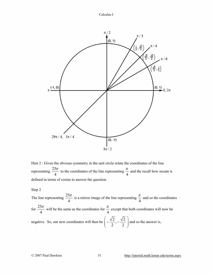
Hint 2 : Given the obvious symmetry in the unit circle relate the coordinates of the line
representing 25
4π
to the coordinates of the line representing 4π
and the recall how secant is
defined in terms of cosine to answer the question. Step 2
The line representing 25
4π
is a mirror image of the line representing 4π
and so the coordinates
for 25
4π
will be the same as the coordinates for 4π
except that both coordinates will now be
negative. So, our new coordinates will then be 2 2,
2 2
− −
and so the answer is,

Calculus I
© 2007 Paul Dawkins 52 http://tutorial.math.lamar.edu/terms.aspx
29 1 1 2sec 2294 2 2sec 24
ππ
= = = − = − −
Review : Solving Trig Equations 1. Without using a calculator find all the solutions to ( )4sin 3 2t = .
Hint 1 : Isolate the sine (with a coefficient of one) on one side of the equation. Step 1 Isolating the sine (with a coefficient of one) on one side of the equation gives,
( ) 1sin 32
t =
Hint 2 : Use your knowledge of the unit circle to determine all the angles in the range [ ]0, 2π for
which sine will have this value. Step 2 Because we’re dealing with sine in this problem and we know that the y-axis represents sine on a unit circle we’re looking for angles that will have a y coordinate of 1
2 . This means we’ll have an angle in the first quadrant and an angle in the second quadrant (that we can use the angle in the first quadrant to find). Here is a unit circle for this situation.

Calculus I
© 2007 Paul Dawkins 53 http://tutorial.math.lamar.edu/terms.aspx
Clearly the angle in the first quadrant is 6π
and by some basic symmetry we can see that the
terminal line for the second angle must form an angle of 6π
with the negative x-axis as shown
above and so it will be : 5
6 6π π
π − = .
Hint 3 : Using the two angles above write down all the angles for which sine will have this value and use these to write down all the solutions to the equation. Step 3 From the discussion in the notes for this section we know that once we have these two angles we can get all possible angles by simply adding “ 2 nπ+ for 0, 1, 2,n = ± ± … ” onto each of these. This then means that we must have,

Calculus I
© 2007 Paul Dawkins 54 http://tutorial.math.lamar.edu/terms.aspx
53 2 OR 3 2 0, 1, 2,6 6
t n t n nπ ππ π= + = + = ± ± …
Finally, to get all the solutions to the equation all we need to do is divide both sides by 3.
2 5 2OR 0, 1, 2,18 3 18 3
n nt t nπ π π π= + = + = ± ± …
2. Without using a calculator find the solution(s) to ( )4sin 3 2t = that are in 40,3π
.
Hint 1 : First, find all the solutions to the equation without regard to the given interval. Step 1 Because we found all the solutions to this equation in Problem 1 of this section we’ll just list the result here. For full details on how these solutions were obtained please see the solution to Problem 1. All solutions to the equation are,
2 5 2OR 0, 1, 2,18 3 18 3
n nt t nπ π π π= + = + = ± ± …
Hint 2 : Now all we need to do is plug in values of n to determine which solutions will actually fall in this interval. Step 2 Note that because at least some of the solutions will have a denominator of 18 it will probably be convenient to also have the interval written in terms of fractions with denominators of 18. Doing this will make it much easier to identify solutions that fall inside the interval so,
4 240, 0,3 18π π =
With the interval written in this form, if our potential solutions have a denominator of 18, all we need to do is compare numerators. As long as the numerators are positive and less than 24π we’ll know that the solution is in the interval. Also, in order to quickly determine the solution for particular values of n it will be much easier to have both fractions in the solutions have denominators of 18. So the solutions, written in this form, are.
Calculus I
© 2007 Paul Dawkins 55 http://tutorial.math.lamar.edu/terms.aspx
12 5 12OR 0, 1, 2,18 18 18 18
n nt t nπ π π π= + = + = ± ± …
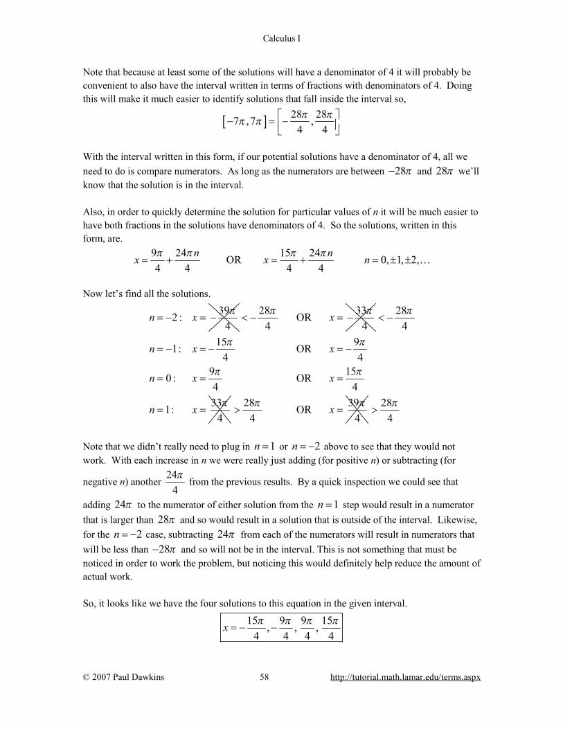
Now let’s find all the solutions. First notice that, in this case, if we plug in negative values of n we will get negative solutions and these will not be in the interval and so there is no reason to even try these. So, let’s start at 0n = and see what we get.
50 : OR18 1813 171: OR18 18252 :18
n t t
n t t
n t
π π
π π
π
= = =
= = =
= =24 29OR18 18
tπ π> =
2418
π>
Note that we didn’t really need to plug in 2n = above to see that they would not work. With
each increase in n we were really just adding another 1218
π onto the previous results and by a
quick inspection we could see that adding 12π to the numerator of either solution from the 1n = step would result in a numerator that is larger than 24π and so would result in a solution that is outside of the interval. This is not something that must be noticed in order to work the problem, but noticing this would definitely help reduce the amount of actual work. So, it looks like we have the four solutions to this equation in the given interval.
5 13 17, , ,18 18 18 18
t π π π π=
3. Without using a calculator find all the solutions to 2cos 2 03x + =
.
Hint 1 : Isolate the cosine (with a coefficient of one) on one side of the equation. Step 1 Isolating the cosine (with a coefficient of one) on one side of the equation gives,
2cos3 2x = −
Calculus I
© 2007 Paul Dawkins 56 http://tutorial.math.lamar.edu/terms.aspx
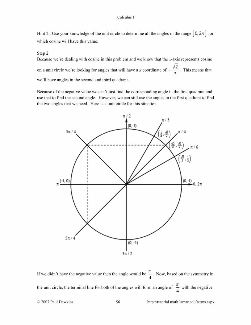
Hint 2 : Use your knowledge of the unit circle to determine all the angles in the range [ ]0,2π for
which cosine will have this value. Step 2 Because we’re dealing with cosine in this problem and we know that the x-axis represents cosine
on a unit circle we’re looking for angles that will have a x coordinate of 2
2− . This means that
we’ll have angles in the second and third quadrant. Because of the negative value we can’t just find the corresponding angle in the first quadrant and use that to find the second angle. However, we can still use the angles in the first quadrant to find the two angles that we need. Here is a unit circle for this situation.
If we didn’t have the negative value then the angle would be 4π
. Now, based on the symmetry in
the unit circle, the terminal line for both of the angles will form an angle of 4π
with the negative

Calculus I
© 2007 Paul Dawkins 57 http://tutorial.math.lamar.edu/terms.aspx
x-axis. The angle in the second quadrant will then be 3
4 4π π
π − = and the angle in the third
quadrant will be 5
4 4π π
π + = .
Hint 3 : Using the two angles above write down all the angles for which cosine will have this value and use these to write down all the solutions to the equation. Step 3 From the discussion in the notes for this section we know that once we have these two angles we can get all possible angles by simply adding “ 2 nπ+ for 0, 1, 2,n = ± ± … ” onto each of these. This then means that we must have,
3 52 OR 2 0, 1, 2,3 4 3 4x xn n nπ π
π π= + = + = ± ± …
Finally, to get all the solutions to the equation all we need to do is multiply both sides by 3.
9 156 OR 6 0, 1, 2,4 4
x n x n nπ ππ π= + = + = ± ± …
4. Without using a calculator find the solution(s) to 2cos 2 03x + =
that are in [ ]7 ,7π π− .
Hint 1 : First, find all the solutions to the equation without regard to the given interval. Step 1 Because we found all the solutions to this equation in Problem 3 of this section we’ll just list the result here. For full details on how these solutions were obtained please see the solution to Problem 3. All solutions to the equation are,
9 156 OR 6 0, 1, 2,4 4
x n x n nπ ππ π= + = + = ± ± …
Hint 2 : Now all we need to do is plug in values of n to determine which solutions will actually fall in this interval. Step 2
Calculus I
© 2007 Paul Dawkins 58 http://tutorial.math.lamar.edu/terms.aspx
Note that because at least some of the solutions will have a denominator of 4 it will probably be convenient to also have the interval written in terms of fractions with denominators of 4. Doing this will make it much easier to identify solutions that fall inside the interval so,
[ ] 28 287 ,7 ,4 4π π
π π − = −
With the interval written in this form, if our potential solutions have a denominator of 4, all we need to do is compare numerators. As long as the numerators are between 28π− and 28π we’ll know that the solution is in the interval. Also, in order to quickly determine the solution for particular values of n it will be much easier to have both fractions in the solutions have denominators of 4. So the solutions, written in this form, are.
9 24 15 24OR 0, 1, 2,4 4 4 4
n nx x nπ π π π= + = + = ± ± …
Now let’s find all the solutions.
392 :4
n x π= − = −
28 33OR4 4
xπ π< − = −
284
15 91: OR4 4
9 150 : OR4 4331:
4
n x x
n x x
n x
π
π π
π π
π
< −
= − = − = −
= = =
= =28 39OR
4 4xπ π
> =28
4π
>
Note that we didn’t really need to plug in 1n = or 2n = − above to see that they would not work. With each increase in n we were really just adding (for positive n) or subtracting (for
negative n) another 24
4π
from the previous results. By a quick inspection we could see that
adding 24π to the numerator of either solution from the 1n = step would result in a numerator that is larger than 28π and so would result in a solution that is outside of the interval. Likewise, for the 2n = − case, subtracting 24π from each of the numerators will result in numerators that will be less than 28π− and so will not be in the interval. This is not something that must be noticed in order to work the problem, but noticing this would definitely help reduce the amount of actual work. So, it looks like we have the four solutions to this equation in the given interval.
15 9 9 15, , ,4 4 4 4
x π π π π= − −

Calculus I
© 2007 Paul Dawkins 59 http://tutorial.math.lamar.edu/terms.aspx
5. Without using a calculator find the solution(s) to ( )4cos 6 12z = that are in 0,2π
.
Hint 1 : Find all the solutions to the equation without regard to the given interval. The first step in this process is to isolate the cosine (with a coefficient of one) on one side of the equation. Step 1 Isolating the cosine (with a coefficient of one) on one side of the equation gives,
( ) 12 2 3 3cos 64 4 2
z = = =
Notice that we needed to do a little simplification of the root to get the value into a more recognizable form. This kind of simplification is usually a good thing to do. Hint 2 : Use your knowledge of the unit circle to determine all the angles in the range [ ]0, 2π for
which cosine will have this value. Step 2 Because we’re dealing with cosine in this problem and we know that the x-axis represents cosine
on a unit circle we’re looking for angles that will have a x coordinate of 3
2. This means we’ll
have an angle in the first quadrant and an angle in the fourth quadrant (that we can use the angle in the first quadrant to find). Here is a unit circle for this situation.

Calculus I
© 2007 Paul Dawkins 60 http://tutorial.math.lamar.edu/terms.aspx
Clearly the angle in the first quadrant is 6π
and by some basic symmetry we can see that the
terminal line for the second angle must form an angle of 6π
with the positive x-axis as shown
above and so it will be : 112
6 6π π
π − = .
Note that you don’t really need a positive angle for the second one. If you wanted to you could
just have easily used 6π
− for the second angle. There is nothing wrong with this and you’ll get
the same solutions in the end. The reason we chose to go with the positive angle is simply to avoid inadvertently losing the minus sign on the second solution at some point in the future. That kind of mistake is easy to make on occasion and by using positive angles here we will not need to worry about making it.
Calculus I
© 2007 Paul Dawkins 61 http://tutorial.math.lamar.edu/terms.aspx
Hint 3 : Using the two angles above write down all the angles for which cosine will have this value and use these to write down all the solutions to the equation. Step 3 From the discussion in the notes for this section we know that once we have these two angles we can get all possible angles by simply adding “ 2 nπ+ for 0, 1, 2,n = ± ± … ” onto each of these. This then means that we must have,
116 2 OR 6 2 0, 1, 2,6 6
z n z n nπ ππ π= + = + = ± ± …
Finally, to get all the solutions to the equation all we need to do is divide both sides by 6.
11OR 0, 1, 2,36 3 36 3
n nz z nπ π π π= + = + = ± ± …
Hint 4 : Now all we need to do is plug in values of n to determine which solutions will actually fall in the given interval. Step 4 Note that because at least some of the solutions will have a denominator of 36 it will probably be convenient to also have the interval written in terms of fractions with denominators of 36. Doing this will make it much easier to identify solutions that fall inside the interval so,
180, 0,2 36π π =
With the interval written in this form, if our potential solutions have a denominator of 36, all we need to do is compare numerators. As long as the numerators are positive and less than 18π we’ll know that the solution is in the interval. Also, in order to quickly determine the solution for particular values of n it will be much easier to have both fractions in the solutions have denominators of 36. So the solutions, written in this form, are.
12 11 12OR 0, 1, 2,36 36 36 36
n nz z nπ π π π= + = + = ± ± …
Now let’s find all the solutions. First notice that, in this case, if we plug in negative values of n we will get negative solutions and these will not be in the interval and so there is no reason to even try these. So, let’s start at 0n = and see what we get.

Calculus I
© 2007 Paul Dawkins 62 http://tutorial.math.lamar.edu/terms.aspx
110 : OR36 3613 231: OR36 36
n z z
n z z
π π
π π
= = =
= = =1836
π>
There are a couple of things we should note before proceeding. First, it is important to understand both solutions from a given value of n will not necessarily be in the given interval. It is completely possible, as this problem shows, that we will only get one or the other solution from a given value of n to fall in the given interval.
Next notice that with each increase in n we were really just adding another 1236
π onto the
previous results and by a quick inspection we could see that adding 12π to the numerator of the first solution from the 1n = step would result in a numerator that is larger than 18π and so would result in a solution that is outside of the interval. Therefore, there was no reason to plug in
2n = into the first set of solutions. Of course, we also didn’t plug 2n = into the second set because once we’ve gotten out of the interval adding anything else on will remain out of the interval. So, it looks like we have the three solutions to this equation in the given interval.
11 13, ,36 36 36
z π π π=
6. Without using a calculator find the solution(s) to 32sin 3 02y + =
that are in
7 ,03π −
.
Hint 1 : Find all the solutions to the equation without regard to the given interval. The first step in this process is to isolate the sine (with a coefficient of one) on one side of the equation. Step 1 Isolating the sine (with a coefficient of one) on one side of the equation gives,
3 3sin2 2y = −
Hint 2 : Use your knowledge of the unit circle to determine all the angles in the range [ ]0, 2π for
which cosine will have this value. Step 2
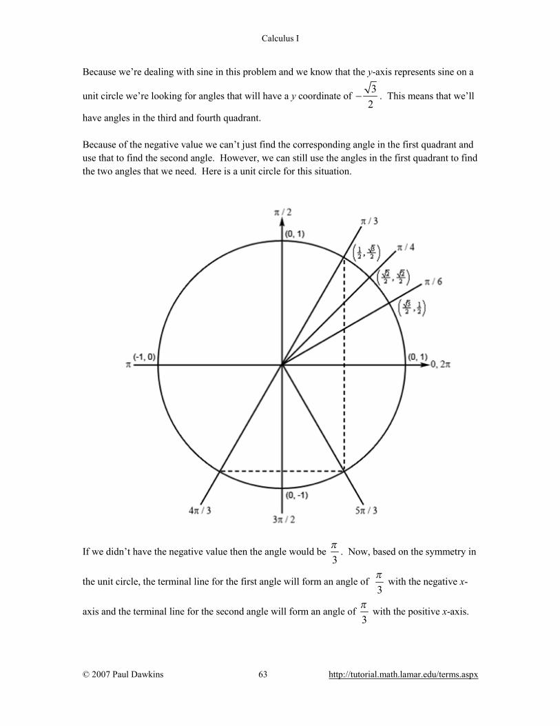
Calculus I
© 2007 Paul Dawkins 63 http://tutorial.math.lamar.edu/terms.aspx
Because we’re dealing with sine in this problem and we know that the y-axis represents sine on a
unit circle we’re looking for angles that will have a y coordinate of 3
2− . This means that we’ll
have angles in the third and fourth quadrant. Because of the negative value we can’t just find the corresponding angle in the first quadrant and use that to find the second angle. However, we can still use the angles in the first quadrant to find the two angles that we need. Here is a unit circle for this situation.
If we didn’t have the negative value then the angle would be 3π
. Now, based on the symmetry in
the unit circle, the terminal line for the first angle will form an angle of 3π
with the negative x-
axis and the terminal line for the second angle will form an angle of 3π
with the positive x-axis.

Calculus I
© 2007 Paul Dawkins 64 http://tutorial.math.lamar.edu/terms.aspx
The angle in the third quadrant will then be 4
3 3π π
π + = and the angle in the fourth quadrant
will be 52
3 3π π
π − = .
Note that you don’t really need a positive angle for the second one. If you wanted to you could
just have easily used 3π
− for the second angle. There is nothing wrong with this and you’ll get
the same solutions in the end. The reason we chose to go with the positive angle is simply to avoid inadvertently losing the minus sign on the second solution at some point in the future. That kind of mistake is easy to make on occasion and by using positive angles here we will not need to worry about making it. Hint 3 : Using the two angles above write down all the angles for which sine will have this value and use these to write down all the solutions to the equation. Step 3 From the discussion in the notes for this section we know that once we have these two angles we can get all possible angles by simply adding “ 2 nπ+ for 0, 1, 2,n = ± ± … ” onto each of these. This then means that we must have,
3 4 3 52 OR 2 0, 1, 2,2 3 2 3y yn n nπ π
π π= + = + = ± ± …
Finally, to get all the solutions to the equation all we need to do is multiply both sides by 23
.
8 4 10 4OR 0, 1, 2,9 3 9 3
n ny y nπ π π π= + = + = ± ± …
Hint 4 : Now all we need to do is plug in values of n to determine which solutions will actually fall in the given interval. Step 4 Note that because at least some of the solutions will have a denominator of 9 it will probably be convenient to also have the interval written in terms of fractions with denominators of 9. Doing this will make it much easier to identify solutions that fall inside the interval so,
7 21,0 ,03 9π π − = −
With the interval written in this form, if our potential solutions have a denominator of 9, all we need to do is compare numerators. As long as the numerators are negative and greater than
21π− we’ll know that the solution is in the interval.
Calculus I
© 2007 Paul Dawkins 65 http://tutorial.math.lamar.edu/terms.aspx
Also, in order to quickly determine the solution for particular values of n it will be much easier to have both fractions in the solutions have denominators of 9. So the solutions, written in this form, are.
8 12 10 12OR 0, 1, 2,9 9 9 9
n ny y nπ π π π= + = + = ± ± …
Now let’s find all the solutions. First notice that, in this case, if we plug in positive values of n or zero we will get positive solutions and these will not be in the interval and so there is no reason to even try these. So, let’s start at 1n = − and see what we get.
4 21: OR9 9
16 142 : OR9 9
n y y
n y y
π π
π π
= − = − = −
= − = − = −
Notice that with each increase (in the negative sense anyway) in n we were really just subtracting
another 12
9π
from the previous results and by a quick inspection we could see that subtracting
12π from either of the numerators from the 2n = − solutions the numerators will be less than 21π− and so will be out of the interval. There is no reason to write down the 3n = − solutions
since we know that they will not be in the given interval. So, it looks like we have the four solutions to this equation in the given interval.
16 14 4 2, , ,9 9 9 9
y π π π π= − − − −
7. Without using a calculator find the solution(s) to ( )8 tan 2 5 3x − = that are in 3,
2 2π π −
.
Hint 1 : Find all the solutions to the equation without regard to the given interval. The first step in this process is to isolate the tangent (with a coefficient of one) on one side of the equation. Step 1 Isolating the tangent (with a coefficient of one) on one side of the equation gives, ( )tan 2 1x = Hint 2 : Determine all the angles in the range [ ]0, 2π for which tangent will have this value.
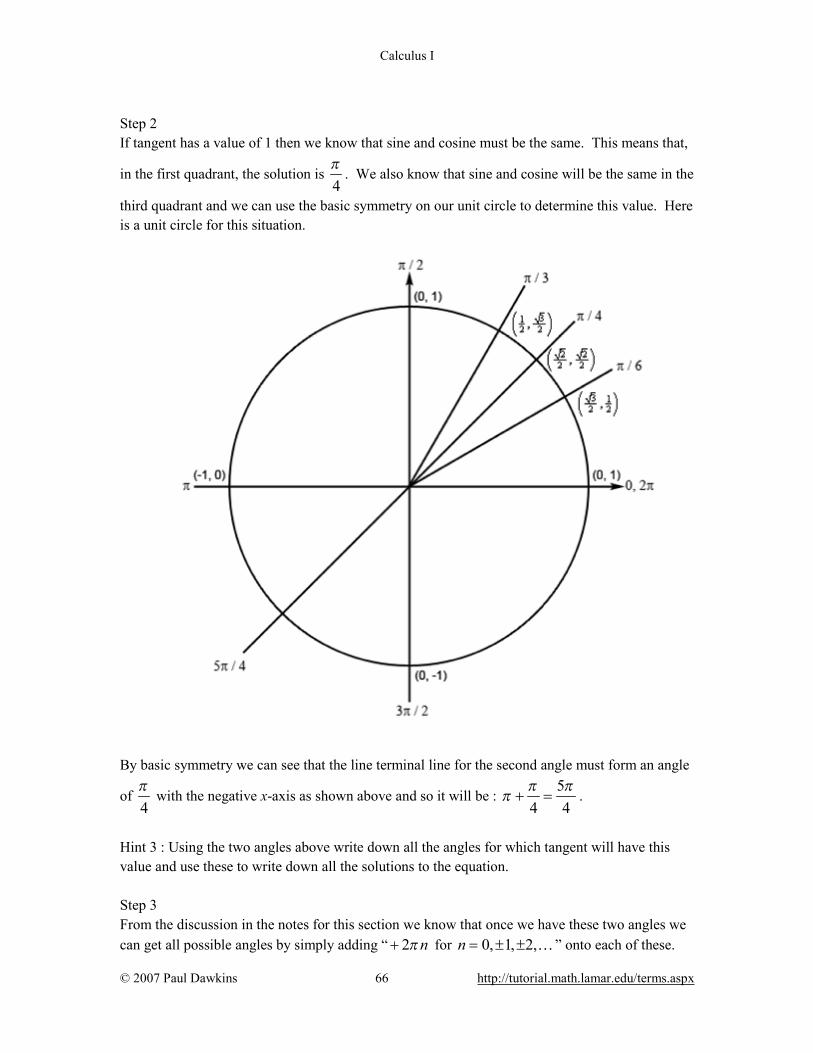
Calculus I
© 2007 Paul Dawkins 66 http://tutorial.math.lamar.edu/terms.aspx
Step 2 If tangent has a value of 1 then we know that sine and cosine must be the same. This means that,
in the first quadrant, the solution is 4π
. We also know that sine and cosine will be the same in the
third quadrant and we can use the basic symmetry on our unit circle to determine this value. Here is a unit circle for this situation.
By basic symmetry we can see that the line terminal line for the second angle must form an angle
of 4π
with the negative x-axis as shown above and so it will be : 5
4 4π π
π + = .
Hint 3 : Using the two angles above write down all the angles for which tangent will have this value and use these to write down all the solutions to the equation. Step 3 From the discussion in the notes for this section we know that once we have these two angles we can get all possible angles by simply adding “ 2 nπ+ for 0, 1, 2,n = ± ± … ” onto each of these.

Calculus I
© 2007 Paul Dawkins 67 http://tutorial.math.lamar.edu/terms.aspx
This then means that we must have,
52 2 OR 2 2 0, 1, 2,4 4
x n x n nπ ππ π= + = + = ± ± …
Finally, to get all the solutions to the equation all we need to do is divide both sides by 2.
5OR 0, 1, 2,8 8
x n x n nπ ππ π= + = + = ± ± …
Hint 4 : Now all we need to do is plug in values of n to determine which solutions will actually fall in the given interval. Step 4 Note that because at least some of the solutions will have a denominator of 8 it will probably be convenient to also have the interval written in terms of fractions with denominators of 8. Doing this will make it much easier to identify solutions that fall inside the interval so,
3 4 12, ,2 2 8 8π π π π − = −
With the interval written in this form, if our potential solutions have a denominator of 8, all we need to do is compare numerators. As long as the numerators are between 4π− and 12π we’ll know that the solution is in the interval. Also, in order to quickly determine the solution for particular values of n it will be much easier to have both fractions in the solutions have denominators of 8. So the solutions, written in this form, are.
8 5 8OR 0, 1, 2,8 8 8 8
n nx x nπ π π π= + = + = ± ± …
Now let’s find all the solutions.
71:8
n x π= − = −
4 3OR8 8
50 : OR8 89 131: OR8 8
x
n x x
n x x
π π
π π
π π
< − = −
= = =
= = =12
8π
>
There are a couple of things we should note before proceeding. First, it is important to understand both solutions from a given value of n will not necessarily be in the given interval. It

Calculus I
© 2007 Paul Dawkins 68 http://tutorial.math.lamar.edu/terms.aspx
is completely possible, as this problem shows, that we will only get one or the other solution from a given value of n to fall in the given interval. Next notice that with each increase in n we were really just adding/subtracting (depending upon
the sign of n) another 88π
from the previous results and by a quick inspection we could see that
adding 8π to the numerator of the 1n = solutions would result in numerators that are larger than 12π and so would result in solutions that are outside of the interval. Likewise, subtracting 8π from the 1n = − solutions would result in numerators that are smaller than 4π− and so would result in solutions that are outside the interval. Therefore, there is no reason to even go past the values of n listed here. So, it looks like we have the four solutions to this equation in the given interval.
3 5 9, , ,8 8 8 8
x π π π π= −
8. Without using a calculator find the solution(s) to ( )16 9sin 7 4x= − − that are in 92 ,4π
π − .
Hint 1 : Find all the solutions to the equation without regard to the given interval. The first step in this process is to isolate the sine (with a coefficient of one) on one side of the equation. Step 1 Isolating the sine (with a coefficient of one) on one side of the equation gives,
( ) 20sin 7 19
x = − < −
Okay, at this point we can stop all work. We know that 1 sin 1θ− ≤ ≤ for any argument and so in this case there is no solution. This will happen on occasion and we shouldn’t get to excited about it when it happens.
9. Without using a calculator find the solution(s) to 3 tan 5 44t + =
that are in [ ]0, 4π .
Hint 1 : Find all the solutions to the equation without regard to the given interval. The first step in this process is to isolate the tangent (with a coefficient of one) on one side of the equation.
Calculus I
© 2007 Paul Dawkins 69 http://tutorial.math.lamar.edu/terms.aspx
Step 1 Isolating the tangent (with a coefficient of one) on one side of the equation gives,
1tan4 3t = −
Hint 2 : Determine all the angles in the range [ ]0, 2π for which tangent will have this value.
Step 2 To get the first angle here let’s recall the definition of tangent in terms of sine and cosine.
( )( )
4
4
sin 1tan4 cos 3
t
tt = = −
Now, because of the section we’re in, we know that the angle must be one of the “standard”
angles and from a quick look at a unit circle (shown below) we know that for 6π
we will have,
( )( )
6
6
1sin 12cos 3 3
2
π
π = =
So, if we had a positive value on the tangent we’d have the first angle. We do have a negative value however, but this work will allow us to get the two angles we’re after. Because the value is negative this simply means that the sine and cosine must have the same values that they have for
6π
except that one must be positive and the other must be negative. This means that the angles
that we’re after must be in the second and fourth quadrants. Here is a unit circle for this situation.

Calculus I
© 2007 Paul Dawkins 70 http://tutorial.math.lamar.edu/terms.aspx
By basic symmetry we can see that the terminal line for the angle in the second quadrant must
form an angle of 6π
with the negative x-axis and the terminal line in the fourth quadrant must
form an angle of 6π
with the positive x-axis as shown above. The angle in the second quadrant
will then be : 5
6 6π π
π − = while the angle in the fourth quadrant will be 112
6 6π π
π − = .
Note that you don’t really need a positive angle for the second one. If you wanted to you could
just have easily used 6π
− for the second angle. There is nothing wrong with this and you’ll get
the same solutions in the end. The reason we chose to go with the positive angle is simply to avoid inadvertently losing the minus sign on the second solution at some point in the future. That kind of mistake is easy to make on occasion and by using positive angles here we will not need to worry about making it.
Calculus I
© 2007 Paul Dawkins 71 http://tutorial.math.lamar.edu/terms.aspx
Hint 3 : Using the two angles above write down all the angles for which tangent will have this value and use these to write down all the solutions to the equation. Step 3 From the discussion in the notes for this section we know that once we have these two angles we can get all possible angles by simply adding “ 2 nπ+ for 0, 1, 2,n = ± ± … ” onto each of these. This then means that we must have,
5 112 OR 2 0, 1, 2,4 6 4 6t tn n nπ π
π π= + = + = ± ± …
Finally, to get all the solutions to the equation all we need to do is multiply both sides by 4.
10 228 OR 8 0, 1, 2,3 3
t n t n nπ ππ π= + = + = ± ± …
Hint 4 : Now all we need to do is plug in values of n to determine which solutions will actually fall in the given interval. Step 4 Note that because at least some of the solutions will have a denominator of 3 it will probably be convenient to also have the interval written in terms of fractions with denominators of 3. Doing this will make it much easier to identify solutions that fall inside the interval so,
[ ] 120, 4 0,3π
π =
With the interval written in this form, if our potential solutions have a denominator of 3, all we need to do is compare numerators. As long as the numerators are positive and less than 12π we’ll know that the solution is in the interval. Also, in order to quickly determine the solution for particular values of n it will be much easier to have both fractions in the solutions have denominators of 3. So the solutions, written in this form, are.
10 24 22 24OR 0, 1, 2,3 3 3 3
n nt t nπ π π π= + = + = ± ± …
Now let’s find all the solutions. First notice that, in this case, if we plug in negative values of n we will get negative solutions and these will not be in the interval and so there is no reason to
even try these. Next, notice that for any positive n we will be adding 24
3π
onto a positive
quantity and so are guaranteed to be greater than 12
3π
and so will out of the given interval. This
Calculus I
© 2007 Paul Dawkins 72 http://tutorial.math.lamar.edu/terms.aspx
leaves 0n = and for this one we can notice that the only solution that will fall in the given interval is then,
103π
Before leaving this problem let’s note that on occasion we will only get a single solution out of all the possible solutions that will fall in the given interval. So, don’t get excited about it if this should happen.
10. Without using a calculator find the solution(s) to ( )3 csc 9 7 5z − = − that are in
4,3 9π π −
.
Hint 1 : Find all the solutions to the equation without regard to the given interval. The first step in this process is to isolate the cosecant (with a coefficient of one) on one side of the equation. Step 1 Isolating the cosecant (with a coefficient of one) on one side of the equation gives,
( ) 2csc 93
z =
Hint 2 : We need to determine all the angles in the range [ ]0, 2π for which cosecant will have
this value. The best way to do this is to rewrite this equation into one in terms of a different trig function that we can more easily deal with. Step 2 The best way to do this is to recall the definition of cosecant in terms of sine and rewrite the equation in terms sine instead as that will be easier to deal with. Doing this gives,
( ) ( ) ( )1 2 3csc 9 sin 9sin 9 23
z zz
= = ⇒ =
The solution(s) to the equation with sine in it are the same as the solution(s) to the equation with cosecant in it and so let’s work with that instead. At this point we are now dealing with sine and we know that the y-axis represents sine on a unit
circle. So we’re looking for angles that will have a y coordinate of 3
2. This means we’ll have
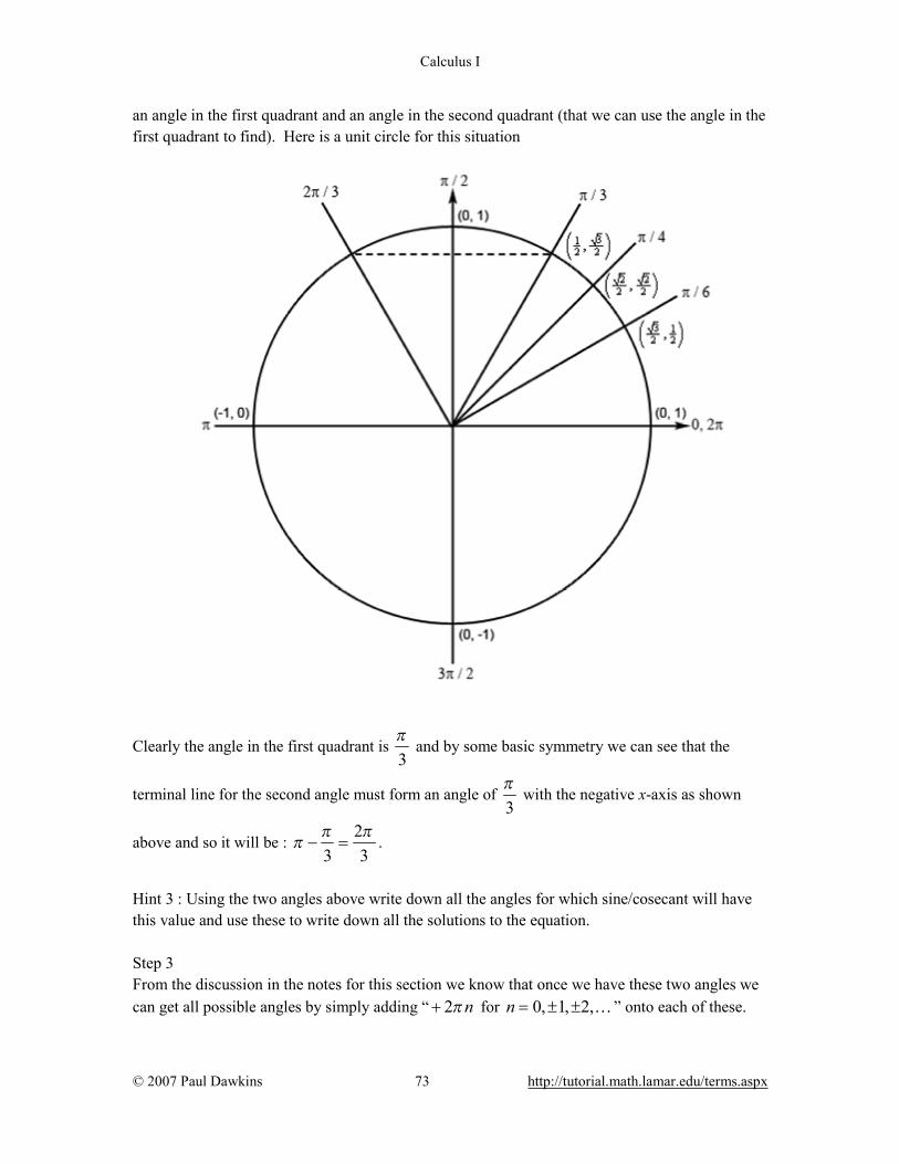
Calculus I
© 2007 Paul Dawkins 73 http://tutorial.math.lamar.edu/terms.aspx
an angle in the first quadrant and an angle in the second quadrant (that we can use the angle in the first quadrant to find). Here is a unit circle for this situation
Clearly the angle in the first quadrant is 3π
and by some basic symmetry we can see that the
terminal line for the second angle must form an angle of 3π
with the negative x-axis as shown
above and so it will be : 2
3 3π π
π − = .
Hint 3 : Using the two angles above write down all the angles for which sine/cosecant will have this value and use these to write down all the solutions to the equation. Step 3 From the discussion in the notes for this section we know that once we have these two angles we can get all possible angles by simply adding “ 2 nπ+ for 0, 1, 2,n = ± ± … ” onto each of these.

Calculus I
© 2007 Paul Dawkins 74 http://tutorial.math.lamar.edu/terms.aspx
This then means that we must have, 29 2 OR 9 2 0, 1, 2,
3 3z n z n nπ π
π π= + = + = ± ± …
Finally, to get all the solutions to the equation all we need to do is divide both sides by 9.
2 2 2OR 0, 1, 2,27 9 27 9
n nz z nπ π π π= + = + = ± ± …
Hint 4 : Now all we need to do is plug in values of n to determine which solutions will actually fall in the given interval. Step 4 Note that because at least some of the solutions will have a denominator of 27 it will probably be convenient to also have the interval written in terms of fractions with denominators of 27. Doing this will make it much easier to identify solutions that fall inside the interval so,
4 9 12, ,3 9 27 27π π π π − = −
With the interval written in this form, if our potential solutions have a denominator of 27, all we need to do is compare numerators. As long as the numerators are between 9π− and 12π we’ll know that the solution is in the interval. Also, in order to quickly determine the solution for particular values of n it will be much easier to have both fractions in the solutions have denominators of 27. So the solutions, written in this form, are.
6 2 6OR 0, 1, 2,27 27 27 27
n nz z nπ π π π= + = + = ± ± …
Now let’s find all the solutions.
5 41: OR27 27
20 : OR27 277 81: OR27 27
n z z
n z z
n z z
π π
π π
π π
= − = − = −
= = =
= = =
Notice that with each increase in n we were really just adding/subtracting (depending upon the
sign of n) another 627π
from the previous results and by a quick inspection we could see that
adding 6π to the numerator of the 1n = solutions would result in numerators that are larger than 12π and so would result in solutions that are outside of the interval. Likewise, subtracting 6π from the 1n = − solutions would result in numerators that are smaller than 9π− and so would
Calculus I
© 2007 Paul Dawkins 75 http://tutorial.math.lamar.edu/terms.aspx
result in solutions that are outside the interval. Therefore, there is no reason to even go past the values of n listed here. So, it looks like we have the six solutions to this equation in the given interval.
5 4 2 7 8, , , , ,27 27 27 27 27 27
x π π π π π π= − −
11. Without using a calculator find the solution(s) to 21 14 cos 65x − = −
that are in
405 ,3π
π
.
Hint 1 : Find all the solutions to the equation without regard to the given interval. The first step in this process is to isolate the cosine (with a coefficient of one) on one side of the equation. Step 1 Isolating the cosine (with a coefficient of one) on one side of the equation gives,
2 1cos5 2x =
Hint 2 : Use your knowledge of the unit circle to determine all the angles in the range [ ]0, 2π for
which cosine will have this value. Step 2 Because we’re dealing with cosine in this problem and we know that the x-axis represents cosine
on a unit circle we’re looking for angles that will have a x coordinate of 12
. This means we’ll
have an angle in the first quadrant and an angle in the fourth quadrant (that we can use the angle in the first quadrant to find). Here is a unit circle for this situation.
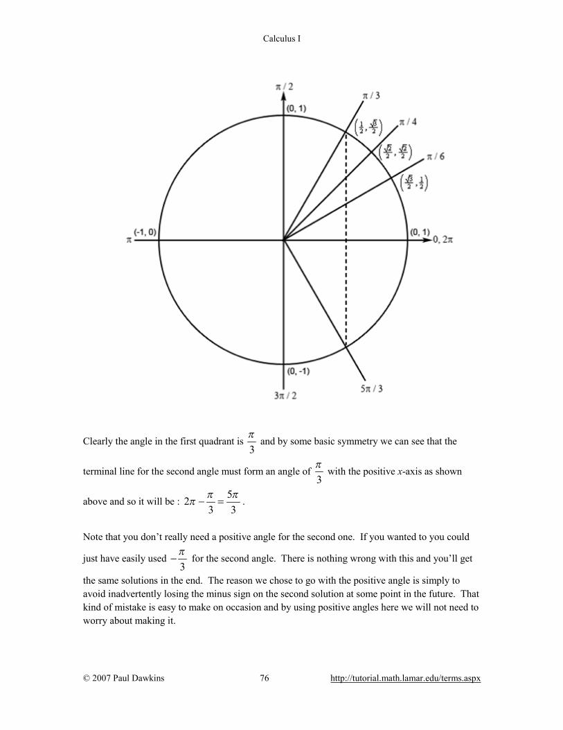
Calculus I
© 2007 Paul Dawkins 76 http://tutorial.math.lamar.edu/terms.aspx
Clearly the angle in the first quadrant is 3π
and by some basic symmetry we can see that the
terminal line for the second angle must form an angle of 3π
with the positive x-axis as shown
above and so it will be : 52
3 3π π
π − = .
Note that you don’t really need a positive angle for the second one. If you wanted to you could
just have easily used 3π
− for the second angle. There is nothing wrong with this and you’ll get
the same solutions in the end. The reason we chose to go with the positive angle is simply to avoid inadvertently losing the minus sign on the second solution at some point in the future. That kind of mistake is easy to make on occasion and by using positive angles here we will not need to worry about making it.
Calculus I
© 2007 Paul Dawkins 77 http://tutorial.math.lamar.edu/terms.aspx
Hint 3 : Using the two angles above write down all the angles for which cosine will have this value and use these to write down all the solutions to the equation. Step 3 From the discussion in the notes for this section we know that once we have these two angles we can get all possible angles by simply adding “ 2 nπ+ for 0, 1, 2,n = ± ± … ” onto each of these. This then means that we must have,
2 2 52 OR 2 0, 1, 2,5 3 5 3x xn n nπ π
π π= + = + = ± ± …
Finally, to get all the solutions to the equation all we need to do is multiply both sides by 52
.
5 255 OR 5 0, 1, 2,6 6
x n x n nπ ππ π= + = + = ± ± …
Hint 4 : Now all we need to do is plug in values of n to determine which solutions will actually fall in the given interval. Step 4 Note that because at least some of the solutions will have a denominator of 6 it will probably be convenient to also have the interval written in terms of fractions with denominators of 6. Doing this will make it much easier to identify solutions that fall inside the interval so,
40 30 805 , ,3 6 6π π π
π =
With the interval written in this form, if our potential solutions have a denominator of 6, all we need to do is compare numerators. As long as the numerators are between 30π and 80π we’ll know that the solution is in the interval. Also, in order to quickly determine the solution for particular values of n it will be much easier to have both fractions in the solutions have denominators of 6. So the solutions, written in this form, are.
5 30 25 30OR 0, 1, 2,6 6 6 6
n nx x nπ π π π= + = + = ± ± …
Now let’s find all the solutions. First notice that, in this case, if we plug in negative values of n we will get negative solutions and these will not be in the interval and so there is no reason to even try these. We can also see from a quick inspection that 0n = will result in solutions that are not in the interval and so let’s start at 1n = and see what we get.

Calculus I
© 2007 Paul Dawkins 78 http://tutorial.math.lamar.edu/terms.aspx
35 551: OR6 6
65 852 : OR6 36
n x x
n x x
π π
π π
= = =
= = =80
6π
>
There are a couple of things we should note before proceeding. First, it is important to understand both solutions from a given value of n will not necessarily be in the given interval. It is completely possible, as this problem shows, that we will only get one or the other solution from a given value of n to fall in the given interval.
Next notice that with each increase in n we were really just adding another 30
6π
onto the
previous results and by a quick inspection we could see that adding 30π to the numerator of the first solution from the 2n = step would result in a numerator that is larger than 80π and so would result in a solution that is outside of the interval. Therefore, there was no reason to plug in
3n = into the first set of solutions. Of course, we also didn’t plug 3n = into the second set because once we’ve gotten out of the interval adding anything else on will remain out of the interval. Finally, unlike most of the problems in this section 0n = did not produce any solutions that were in the given interval. This will happen on occasion so don’t get excited about it when it happens. So, it looks like we have the three solutions to this equation in the given interval.
35 55 65, ,6 6 6
z π π π=
12. Without using a calculator find the solution(s) to 15 17 4cos7y = +
that are in [ ]10 ,15π π
. Hint 1 : Find all the solutions to the equation without regard to the given interval. The first step in this process is to isolate the cosine (with a coefficient of one) on one side of the equation. Step 1 Isolating the cosine (with a coefficient of one) on one side of the equation gives,
1cos7 2y = −
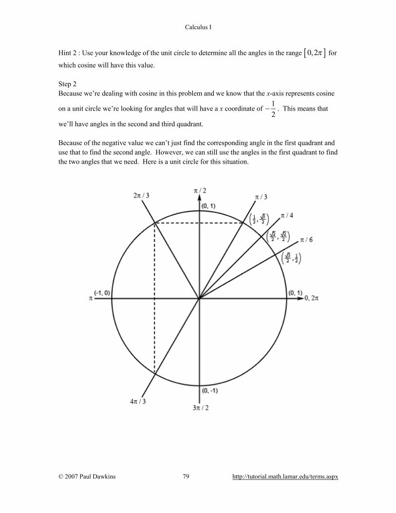
Calculus I
© 2007 Paul Dawkins 79 http://tutorial.math.lamar.edu/terms.aspx
Hint 2 : Use your knowledge of the unit circle to determine all the angles in the range [ ]0,2π for
which cosine will have this value. Step 2 Because we’re dealing with cosine in this problem and we know that the x-axis represents cosine
on a unit circle we’re looking for angles that will have a x coordinate of 12
− . This means that
we’ll have angles in the second and third quadrant. Because of the negative value we can’t just find the corresponding angle in the first quadrant and use that to find the second angle. However, we can still use the angles in the first quadrant to find the two angles that we need. Here is a unit circle for this situation.
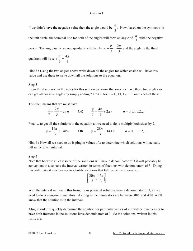
Calculus I
© 2007 Paul Dawkins 80 http://tutorial.math.lamar.edu/terms.aspx
If we didn’t have the negative value then the angle would be 3π
. Now, based on the symmetry in
the unit circle, the terminal line for both of the angles will form an angle of 3π
with the negative
x-axis. The angle in the second quadrant will then be 2
3 3π π
π − = and the angle in the third
quadrant will be 4
3 3π π
π + = .
Hint 3 : Using the two angles above write down all the angles for which cosine will have this value and use these to write down all the solutions to the equation. Step 3 From the discussion in the notes for this section we know that once we have these two angles we can get all possible angles by simply adding “ 2 nπ+ for 0, 1, 2,n = ± ± … ” onto each of these. This then means that we must have,
2 42 OR 2 0, 1, 2,7 3 7 3y yn n nπ π
π π= + = + = ± ± …
Finally, to get all the solutions to the equation all we need to do is multiply both sides by 7.
14 2814 OR 14 0, 1, 2,3 3
y n y n nπ ππ π= + = + = ± ± …
Hint 4 : Now all we need to do is plug in values of n to determine which solutions will actually fall in the given interval. Step 4 Note that because at least some of the solutions will have a denominator of 3 it will probably be convenient to also have the interval written in terms of fractions with denominators of 3. Doing this will make it much easier to identify solutions that fall inside the interval so,
30 45,3 3π π
With the interval written in this form, if our potential solutions have a denominator of 3, all we need to do is compare numerators. As long as the numerators are between 30π and 45π we’ll know that the solution is in the interval. Also, in order to quickly determine the solution for particular values of n it will be much easier to have both fractions in the solutions have denominators of 3. So the solutions, written in this form, are.

Calculus I
© 2007 Paul Dawkins 81 http://tutorial.math.lamar.edu/terms.aspx
14 42 28 42OR 0, 1, 2,3 3 3 3
n ny y nπ π π π= + = + = ± ± …
Now let’s find all the solutions. First notice that, in this case, if we plug in negative values of n we will get negative solutions and these will not be in the interval and so there is no reason to even try these. We can also see from a quick inspection that 0n = will result in solutions that are not in the interval and so let’s start at 1n = and see what we get.
561:3
n x π= =
45 70OR3 3
xπ π> =
453π
>
So, by plugging in 1n = we get solutions that are already outside of the interval and increasing n
will simply mean adding another 42
3π
onto these and so will remain outside of the given
interval. We also noticed earlier than all other value of n will result in solutions outside of the given interval. What all this means is that while there are solutions to the equation none fall inside the given interval and so the official answer would then be no solutions in the given interval.
Review : Solving Trig Equations with Calculators, Part I 1. Find all the solutions to ( )7cos 4 11 10x + = . Use at least 4 decimal places in your work.
Hint 1 : Isolate the cosine (with a coefficient of one) on one side of the equation. Step 1 Isolating the cosine (with a coefficient of one) on one side of the equation gives,
( ) 1cos 47
x = −
Hint 2 : Using a calculator and your knowledge of the unit circle to determine all the angles in the range [ ]0, 2π for which cosine will have this value.
Step 2 First, using our calculator we can see that,
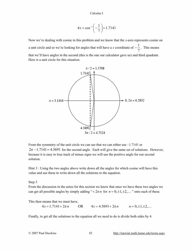
Calculus I
© 2007 Paul Dawkins 82 http://tutorial.math.lamar.edu/terms.aspx
1 14 cos 1.71417
x − = − =
Now we’re dealing with cosine in this problem and we know that the x-axis represents cosine on
a unit circle and so we’re looking for angles that will have a x coordinate of 17
− . This means
that we’ll have angles in the second (this is the one our calculator gave us) and third quadrant. Here is a unit circle for this situation.
From the symmetry of the unit circle we can see that we can either use –1.7141 or 2 1.7141 4.5691π − = for the second angle. Each will give the same set of solutions. However, because it is easy to lose track of minus signs we will use the positive angle for our second solution. Hint 3 : Using the two angles above write down all the angles for which cosine will have this value and use these to write down all the solutions to the equation. Step 3 From the discussion in the notes for this section we know that once we have these two angles we can get all possible angles by simply adding “ 2 nπ+ for 0, 1, 2,n = ± ± … ” onto each of these. This then means that we must have,
4 1.7141 2 OR 4 4.5691 2 0, 1, 2,x n x n nπ π= + = + = ± ± … Finally, to get all the solutions to the equation all we need to do is divide both sides by 4.

Calculus I
© 2007 Paul Dawkins 83 http://tutorial.math.lamar.edu/terms.aspx
0.4285 OR 1.1423 0, 1, 2,2 2n nx x nπ π
= + = + = ± ± …
Note that depending upon the amount of decimals you used here your answers may vary slightly from these due to round off error. Any differences should be slight and only appear around the 4th decimal place or so however.
2. Find the solution(s) to 6 5cos 103x + =
that are in [ ]0,38 . Use at least 4 decimal places in
your work. Hint 1 : Find all the solutions to the equation without regard to the given interval. The first step in this process is to isolate the cosine (with a coefficient of one) on one side of the equation. Step 1 Isolating the cosine (with a coefficient of one) on one side of the equation gives,
4cos3 5x =
Hint 2 : Using a calculator and your knowledge of the unit circle to determine all the angles in the range [ ]0, 2π for which cosine will have this value.
Step 2 First, using our calculator we can see that,
1 4cos 0.64353 5x − = =
Now we’re dealing with cosine in this problem and we know that the x-axis represents cosine on
a unit circle and so we’re looking for angles that will have a x coordinate of 45
. This means that
we’ll have angles in the first (this is the one our calculator gave us) and fourth quadrant. Here is a unit circle for this situation.
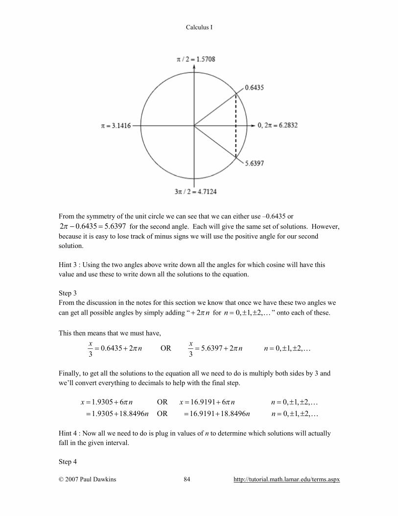
Calculus I
© 2007 Paul Dawkins 84 http://tutorial.math.lamar.edu/terms.aspx
From the symmetry of the unit circle we can see that we can either use –0.6435 or 2 0.6435 5.6397π − = for the second angle. Each will give the same set of solutions. However, because it is easy to lose track of minus signs we will use the positive angle for our second solution. Hint 3 : Using the two angles above write down all the angles for which cosine will have this value and use these to write down all the solutions to the equation. Step 3 From the discussion in the notes for this section we know that once we have these two angles we can get all possible angles by simply adding “ 2 nπ+ for 0, 1, 2,n = ± ± … ” onto each of these. This then means that we must have,
0.6435 2 OR 5.6397 2 0, 1, 2,3 3x xn n nπ π= + = + = ± ± …
Finally, to get all the solutions to the equation all we need to do is multiply both sides by 3 and we’ll convert everything to decimals to help with the final step.
1.9305 6 OR 16.9191 6 0, 1, 2,1.9305 18.8496 OR 16.9191 18.8496 0, 1, 2,
x n x n nn n n
π π= + = + = ± ±= + = + = ± ±
……
Hint 4 : Now all we need to do is plug in values of n to determine which solutions will actually fall in the given interval. Step 4

Calculus I
© 2007 Paul Dawkins 85 http://tutorial.math.lamar.edu/terms.aspx
Now let’s find all the solutions. First notice that, in this case, if we plug in negative values of n we will get negative solutions and these will not be in the interval and so there is no reason to even try these. So, let’s start at 0n = and see what we get.
0 : 1.9305 OR 16.91911: 20.7801 OR 35.7687
n x xn x x
= = == = =
Notice that with each increase in n we were really just adding another 18.8496 onto the previous results and by doing this to the results from the 1n = step we will get solutions that are outside of the interval and so there is no reason to even plug in 2n = . So, it looks like we have the four solutions to this equation in the given interval.
1.9305, 16.9191, 20.7801, 35.7687x =
Note that depending upon the amount of decimals you used here your answers may vary slightly from these due to round off error. Any differences should be slight and only appear around the 4th decimal place or so however.
3. Find all the solutions to 3 6 11sin8t = −
. Use at least 4 decimal places in your work.
Hint 1 : Isolate the sine (with a coefficient of one) on one side of the equation. Step 1 Isolating the sine (with a coefficient of one) on one side of the equation gives,
3sin8 11t =
Hint 2 : Using a calculator and your knowledge of the unit circle to determine all the angles in the range [ ]0, 2π for which sine will have this value.
Step 2 First, using our calculator we can see that,
1 3sin 0.27628 11t − = =
Now we’re dealing with sine in this problem and we know that the y-axis represents sine on a unit
circle and so we’re looking for angles that will have a y coordinate of 3
11. This means that we’ll

Calculus I
© 2007 Paul Dawkins 86 http://tutorial.math.lamar.edu/terms.aspx
have angles in the first (this is the one our calculator gave us) and second quadrant. Here is a unit circle for this situation.
From the symmetry of the unit circle we can see that 0.2762 2.8654π − = is the second angle. Hint 3 : Using the two angles above write down all the angles for which sine will have this value and use these to write down all the solutions to the equation. Step 3 From the discussion in the notes for this section we know that once we have these two angles we can get all possible angles by simply adding “ 2 nπ+ for 0, 1, 2,n = ± ± … ” onto each of these. This then means that we must have,
0.2762 2 OR 2.8654 2 0, 1, 2,8 8t tn n nπ π= + = + = ± ± …
Finally, to get all the solutions to the equation all we need to do is multiply both sides by 8.
2.2096 16 OR 22.9232 16 0, 1, 2,t n t n nπ π= + = + = ± ± … Note that depending upon the amount of decimals you used here your answers may vary slightly from these due to round off error. Any differences should be slight and only appear around the 4th decimal place or so however.
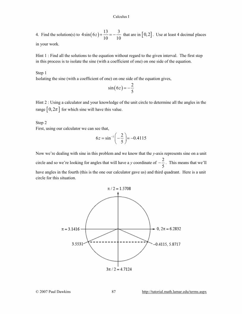
Calculus I
© 2007 Paul Dawkins 87 http://tutorial.math.lamar.edu/terms.aspx
4. Find the solution(s) to ( ) 13 34sin 610 10
z + = − that are in [ ]0,2 . Use at least 4 decimal places
in your work. Hint 1 : Find all the solutions to the equation without regard to the given interval. The first step in this process is to isolate the sine (with a coefficient of one) on one side of the equation. Step 1 Isolating the sine (with a coefficient of one) on one side of the equation gives,
( ) 2sin 65
z = −
Hint 2 : Using a calculator and your knowledge of the unit circle to determine all the angles in the range [ ]0,2π for which sine will have this value.
Step 2 First, using our calculator we can see that,
1 26 sin 0.41155
z − = − = −
Now we’re dealing with sine in this problem and we know that the y-axis represents sine on a unit
circle and so we’re looking for angles that will have a y coordinate of 25
− . This means that we’ll
have angles in the fourth (this is the one our calculator gave us) and third quadrant. Here is a unit circle for this situation.
Calculus I
© 2007 Paul Dawkins 88 http://tutorial.math.lamar.edu/terms.aspx
From the symmetry of the unit circle we can see that the second angle will make an angle of 0.4115 with the negative x-axis and so the second angle will be 0.4115 3.5531π + = . Also, as noted on the unit circle above a positive angle that represents the first angle (i.e. the angle in the fourth quadrant) is 2 0.4115 5.8717π − = . We can use either the positive or the negative angle here and we’ll get the same solutions. However, because it is often easy to lose track of minus signs we will be using the positive angle in the fourth quadrant for our work here. Hint 3 : Using the two angles above write down all the angles for which sine will have this value and use these to write down all the solutions to the equation. Step 3 From the discussion in the notes for this section we know that once we have these two angles we can get all possible angles by simply adding “ 2 nπ+ for 0, 1, 2,n = ± ± … ” onto each of these. This then means that we must have,
6 3.5531 2 OR 6 5.8717 2 0, 1, 2,z n z n nπ π= + = + = ± ± … Finally, to get all the solutions to the equation all we need to do is divide both sides by 6 and we’ll convert everything to decimals to help with the final step.
0.5922 OR 0.9786 0, 1, 2,
3 30.5922 1.0472 OR 0.9786 1.0472 0, 1, 2,
n nz z n
n n n
π π= + = + = ± ±
= + = + = ± ±
…
…
Hint 4 : Now all we need to do is plug in values of n to determine which solutions will actually fall in the given interval. Step 4 Now let’s find all the solutions. First notice that, in this case, if we plug in negative values of n we will get negative solutions and these will not be in the interval and so there is no reason to even try these. So, let’s start at 0n = and see what we get.
0 : 0.5922 OR 0.97861: 1.6394 OR 2.0258
n z zn z z
= = == = = 2>
Notice that with each increase in n we were really just adding another 1.0472 onto the previous results and by doing this to the results from the 1n = step we will get solutions that are outside of the interval and so there is no reason to even plug in 2n = . Also, as we’ve seen in this problem it is completely possible for only one of the solutions from a given interval to be in the given interval so don’t worry about that when it happens. So, it looks like we have the three solutions to this equation in the given interval.
Calculus I
© 2007 Paul Dawkins 89 http://tutorial.math.lamar.edu/terms.aspx
0.5922, 0.9786, 1.6394z =
Note that depending upon the amount of decimals you used here your answers may vary slightly from these due to round off error. Any differences should be slight and only appear around the 4th decimal place or so however.
5. Find the solution(s) to 4 49cos 21sin 09 9z z + =
that are in [ ]10,10− . Use at least 4
decimal places in your work. Hint 1 : Find all the solutions to the equation without regard to the given interval. The first step in this process is to reduce the equation down to a single trig function (with a coefficient of one) on one side of the equation. Step 1 Because we’ve got both a sine and a cosine here it makes some sense to reduce this down to tangent. So, reducing to a tangent (with a coefficient of one) on one side of the equation gives,
4 3tan9 7z = −
Hint 2 : Using a calculator and your knowledge of solving trig equations involving tangents to determine all the angles in the range [ ]0, 2π for which tangent will have this value.
Step 2 First, using our calculator we can see that,
14 3tan 0.40499 7z − = − = −
As we discussed in Example 5 of this section the second angle for equations involving tangent will always be the π plus the first angle. Therefore, ( )0.4049 2.7367π + − = will be the
second angle. Also, because it is very easy to lose track of minus signs we’ll use the fact that we know that any angle plus 2π will give another angle whose terminal line is identical to the original angle to eliminate the minus sign on the first angle. So, another angle that will work for the first angle is
( )2 0.4049 5.8783π + − = . Note that there is nothing wrong with using the negative angle and if
you chose to work with that you will get the same solutions. We are using the positive angle only to make sure we don’t accidentally lose the minus sign on the angle we received from our calculator.
Calculus I
© 2007 Paul Dawkins 90 http://tutorial.math.lamar.edu/terms.aspx
Hint 3 : Using the two angles above write down all the angles for which tangent will have this value and use these to write down all the solutions to the equation. Step 3 From the discussion in the notes for this section we know that once we have these two angles we can get all possible angles by simply adding “ 2 nπ+ for 0, 1, 2,n = ± ± … ” onto each of these. This then means that we must have,
4 42.7367 2 OR 5.8783 2 0, 1, 2,9 9z zn n nπ π= + = + = ± ± …
Finally, to get all the solutions to the equation all we need to do is multiply both sides by 94
and
we’ll convert everything to decimals to help with the final step.
9 96.1576 OR 13.2262 0, 1, 2,
2 26.1576 14.1372 OR 13.2262 14.1372 0, 1, 2,
n nz z n
n n n
π π= + = + = ± ±
= + = + = ± ±
…
…
Hint 4 : Now all we need to do is plug in values of n to determine which solutions will actually fall in the given interval. Step 4 Now let’s find all the solutions.
1: 7.9796 OR 0.9110
0 : 6.1576 OR 13.2262n z zn z z
= − = − = −= = = 10>
Notice that with each increase in n we were really just adding/subtracting (depending on the sign of n) another 14.1372 onto the previous results. A quick inspection of the results above will quickly show us that we don’t need to go any farther and we won’t bother with any other values of n. Also, as we’ve seen in this problem it is completely possible for only one of the solutions from a given interval to be in the given interval so don’t worry about that when it happens. So, it looks like we have the three solutions to this equation in the given interval.
7.9796, 0.9110, 6.1576z = − −
Note that depending upon the amount of decimals you used here your answers may vary slightly from these due to round off error. Any differences should be slight and only appear around the 4th decimal place or so however.
Calculus I
© 2007 Paul Dawkins 91 http://tutorial.math.lamar.edu/terms.aspx
6. Find the solution(s) to 3tan 1 11 2 tan4 4w w − = −
that are in [ ]50,0− . Use at least 4
decimal places in your work. Hint 1 : Find all the solutions to the equation without regard to the given interval. The first step in this process is to isolate the tangent (with a coefficient of one) on one side of the equation. Step 1 Isolating the tangent (with a coefficient of one) on one side of the equation gives,
12tan4 5w =
Hint 2 : Using a calculator and your knowledge of solving trig equations involving tangents to determine all the angles in the range [ ]0, 2π for which tangent will have this value.
Step 2 First, using our calculator we can see that,
1 12tan 1.17604 5w − = =
As we discussed in Example 5 of this section the second angle for equations involving tangent will always be the π plus the first angle. Therefore, 1.1760 4.3176π + = will be the second angle. Hint 3 : Using the two angles above write down all the angles for which tangent will have this value and use these to write down all the solutions to the equation. Step 3 From the discussion in the notes for this section we know that once we have these two angles we can get all possible angles by simply adding “ 2 nπ+ for 0, 1, 2,n = ± ± … ” onto each of these. This then means that we must have,
1.1760 2 OR 4.3176 2 0, 1, 2,4 4w wn n nπ π= + = + = ± ± …
Finally, to get all the solutions to the equation all we need to do is multiply both sides by 4 and we’ll convert everything to decimals to help with the final step.
4.7040 8 OR 17.2704 8 0, 1, 2,4.7040 25.1327 OR 17.2704 25.1327 0, 1, 2,
w n w n nn n n
π π= + = + = ± ±= + = + = ± ±
……
Calculus I
© 2007 Paul Dawkins 92 http://tutorial.math.lamar.edu/terms.aspx
Hint 4 : Now all we need to do is plug in values of n to determine which solutions will actually fall in the given interval. Step 4 Now let’s find all the solutions. First, notice that if we plug in positive n or 0n = we will have positive solutions and these solutions will be out of the interval. Therefore, we’ll start with
1n = − .
1: 20.4287 OR 7.86232 : 45.5614 OR 32.9950
n w wn w w
= − = − = −= − = − = −
Notice that with each increase in n we were really just subtracting another 25.1327 from the previous results. A quick inspection of the results above will quickly show us that we don’t need to go any farther and we won’t bother with any other values of n. So, it looks like we have the four solutions to this equation in the given interval.
45.5614, 32.9950, 20.4287, 7.8623w = − − − −
Note that depending upon the amount of decimals you used here your answers may vary slightly from these due to round off error. Any differences should be slight and only appear around the 4th decimal place or so however.
7. Find the solution(s) to 17 3sec 22z − =
that are in [ ]20,45 . Use at least 4 decimal places
in your work. Hint 1 : Find all the solutions to the equation without regard to the given interval. The first step in this process is to isolate the secant (with a coefficient of one) on one side of the equation. Step 1 Isolating the secant (with a coefficient of one) on one side of the equation gives,
sec 52z =
Hint 2 : Using a calculator and your knowledge of the unit circle to determine all the angles in the range [ ]0, 2π for which secant will have this value. The best way to do this is to rewrite the
equation into one in terms of a different trig function that we can more easily deal with. Step 2 In order to get the solutions it will be much easier to recall the definition of secant in terms of cosine and rewrite the equation into one involving cosine. Doing this gives,
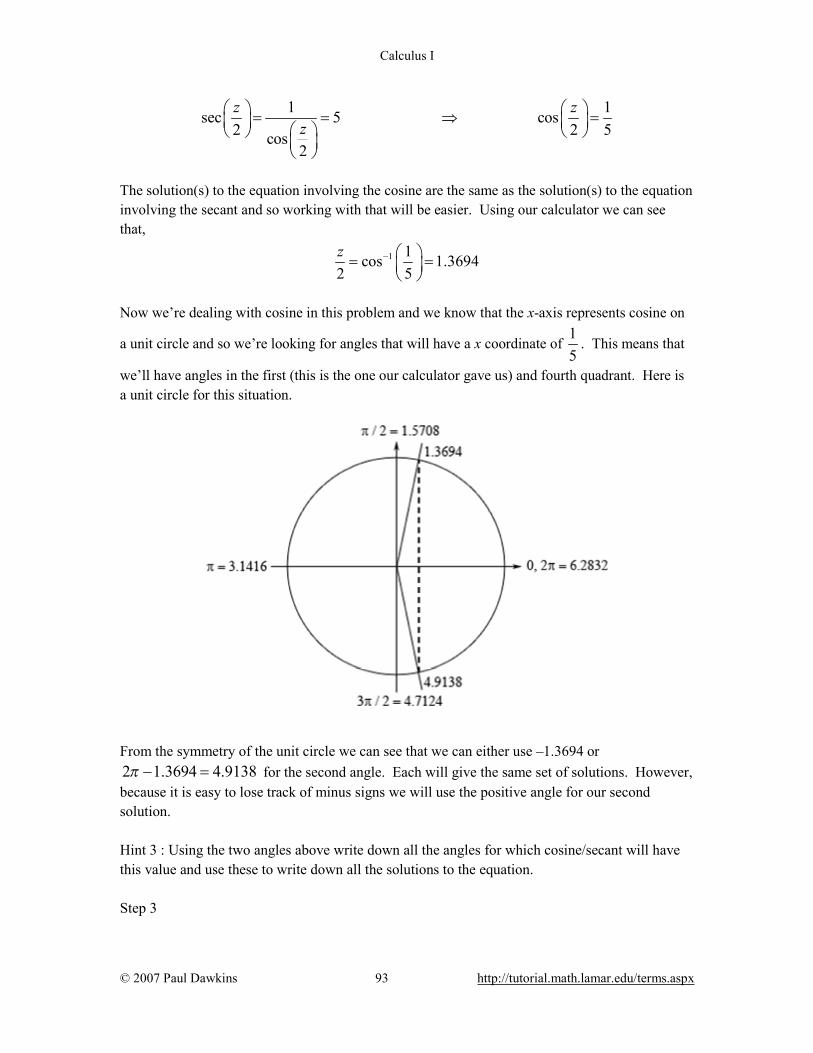
Calculus I
© 2007 Paul Dawkins 93 http://tutorial.math.lamar.edu/terms.aspx
1 1sec 5 cos2 2 5cos
2
z zz
= = ⇒ =
The solution(s) to the equation involving the cosine are the same as the solution(s) to the equation involving the secant and so working with that will be easier. Using our calculator we can see that,
1 1cos 1.36942 5z − = =
Now we’re dealing with cosine in this problem and we know that the x-axis represents cosine on
a unit circle and so we’re looking for angles that will have a x coordinate of 15
. This means that
we’ll have angles in the first (this is the one our calculator gave us) and fourth quadrant. Here is a unit circle for this situation.
From the symmetry of the unit circle we can see that we can either use –1.3694 or 2 1.3694 4.9138π − = for the second angle. Each will give the same set of solutions. However, because it is easy to lose track of minus signs we will use the positive angle for our second solution. Hint 3 : Using the two angles above write down all the angles for which cosine/secant will have this value and use these to write down all the solutions to the equation. Step 3
Calculus I
© 2007 Paul Dawkins 94 http://tutorial.math.lamar.edu/terms.aspx
From the discussion in the notes for this section we know that once we have these two angles we can get all possible angles by simply adding “ 2 nπ+ for 0, 1, 2,n = ± ± … ” onto each of these. This then means that we must have,
1.3694 2 OR 4.9138 2 0, 1, 2,2 2z zn n nπ π= + = + = ± ± …
Finally, to get all the solutions to the equation all we need to do is multiply both sides by 2 and we’ll convert everything to decimals to help with the final step.
2.7388 4 OR 9.8276 4 0, 1, 2,2.7388 12.5664 OR 9.8276 12.5664 0, 1, 2,
z n z n nn n n
π π= + = + = ± ±= + = + = ± ±
……
Hint 4 : Now all we need to do is plug in values of n to determine which solutions will actually fall in the given interval. Step 4 Now let’s find all the solutions. First notice that, in this case, if we plug in negative values of n we will get negative solutions and these will not be in the interval and so there is no reason to even try these. Also note that if we use 0n = we will still not be in the interval and so let’s start things off at 1n = .
1: 15.3052n z= = 20 OR 22.39402 : 27.8716 OR 34.96043: 40.4380 OR 47.5268
zn z zn z z
< == = == = = 45>
Notice that with each increase in n we were really just adding another 12.5664 onto the previous results and by a quick inspection of the results above we can see that we don’t need to go any farther. Also, as we’ve seen in this problem it is completely possible for only one of the solutions from a given interval to be in the given interval so don’t worry about that when it happens. So, it looks like we have the four solutions to this equation in the given interval.
22.3940, 27.8716, 34.9604, 40.4380z =
Note that depending upon the amount of decimals you used here your answers may vary slightly from these due to round off error. Any differences should be slight and only appear around the 4th decimal place or so however.
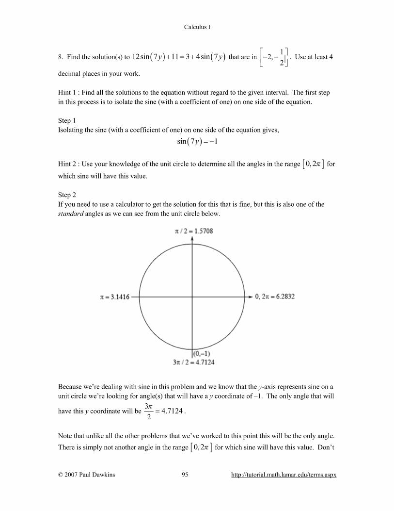
Calculus I
© 2007 Paul Dawkins 95 http://tutorial.math.lamar.edu/terms.aspx
8. Find the solution(s) to ( ) ( )12sin 7 11 3 4sin 7y y+ = + that are in 12,2
− − . Use at least 4
decimal places in your work. Hint 1 : Find all the solutions to the equation without regard to the given interval. The first step in this process is to isolate the sine (with a coefficient of one) on one side of the equation. Step 1 Isolating the sine (with a coefficient of one) on one side of the equation gives, ( )sin 7 1y = − Hint 2 : Use your knowledge of the unit circle to determine all the angles in the range [ ]0,2π for
which sine will have this value. Step 2 If you need to use a calculator to get the solution for this that is fine, but this is also one of the standard angles as we can see from the unit circle below.
Because we’re dealing with sine in this problem and we know that the y-axis represents sine on a unit circle we’re looking for angle(s) that will have a y coordinate of –1. The only angle that will
have this y coordinate will be 3 4.71242π
= .
Note that unlike all the other problems that we’ve worked to this point this will be the only angle. There is simply not another angle in the range [ ]0,2π for which sine will have this value. Don’t
Calculus I
© 2007 Paul Dawkins 96 http://tutorial.math.lamar.edu/terms.aspx
get so locked into the usual case where we get two possible angles in the [ ]0, 2π that when these
single solution cases roll around you decide you must have done something wrong. They happen on occasion and we need to be able to deal with them when they occur. Hint 3 : Using the angle above write down all the angles for which sine will have this value and use these to write down all the solutions to the equation. Step 3 From the discussion in the notes for this section we know that once we have the angle above we can get all possible angles by simply adding “ 2 nπ+ for 0, 1, 2,n = ± ± … ” onto the angle. This then means that we must have,
7 4.7124 2 0, 1, 2,y n nπ= + = ± ± … Finally, to get all the solutions to the equation all we need to do is divide both sides by 7 and we’ll convert everything to decimals to help with the final step.
20.6732 0, 1, 2,
70.6732 0.8976 0, 1, 2,
ny n
n n
π= + = ± ±
= + = ± ±
…
…
Hint 4 : Now all we need to do is plug in values of n to determine which solutions will actually fall in the given interval. Step 4 Now let’s find all the solutions. First notice that, in this case, if we plug in positive values of n or
0n = we will get positive solutions and these will not be in the interval and so there is no reason to even try these. So, let’s start at 1n = − and see what we get.
1: 0.2244n y= − = − 0.52 : 1.1223: 2.0196
n yn y
> −= − = −= − = − 2< −
So, it looks like we have only a single solution to this equation in the given interval.
1.122y = −
Note that depending upon the amount of decimals you used here your answers may vary slightly from these due to round off error. Any differences should be slight and only appear around the 4th decimal place or so however.
Calculus I
© 2007 Paul Dawkins 97 http://tutorial.math.lamar.edu/terms.aspx
9. Find the solution(s) to ( )5 14 tan 8 30x− = that are in [ ]1,1− . Use at least 4 decimal places
in your work. Hint 1 : Find all the solutions to the equation without regard to the given interval. The first step in this process is to isolate the tangent (with a coefficient of one) on one side of the equation. Step 1 Isolating the tangent (with a coefficient of one) on one side of the equation gives,
( ) 25tan 814
x = −
Hint 2 : Using a calculator and your knowledge of solving trig equations involving tangents to determine all the angles in the range [ ]0, 2π for which tangent will have this value.
Step 2 First, using our calculator we can see that,
1 258 tan 1.060314
x − = − = −
As we discussed in Example 5 of this section the second angle for equations involving tangent will always be the π plus the first angle. Therefore, ( )1.0603 2.0813π + − = will be the
second angle. Hint 3 : Using the two angles above write down all the angles for which tangent will have this value and use these to write down all the solutions to the equation. Step 3 From the discussion in the notes for this section we know that once we have these two angles we can get all possible angles by simply adding “ 2 nπ+ for 0, 1, 2,n = ± ± … ” onto each of these. This then means that we must have,
8 1.0603 2 OR 8 2.0813 2 0, 1, 2,x n x n nπ π= − + = + = ± ± … Finally, to get all the solutions to the equation all we need to do is divide both sides by 8 and we’ll convert everything to decimals to help with the final step.
0.1325 OR 0.2602 0, 1, 2,
4 40.1325 0.7854 OR 0.2602 0.7854 0, 1, 2,
n nx x n
n n n
π π= − + = + = ± ±
= − + = + = ± ±
…
…
Calculus I
© 2007 Paul Dawkins 98 http://tutorial.math.lamar.edu/terms.aspx
Hint 4 : Now all we need to do is plug in values of n to determine which solutions will actually fall in the given interval. Step 4 Now let’s find all the solutions.
1: 0.9179 OR 0.5252
0 : 0.1325 OR 0.26021: 0.6529 OR 1.0456
n x xn x xn x x
= − = − = −= = − == = = 1>
Notice that with each increase in n we were really just adding/subtracting another 0.7854 from the previous results. A quick inspection of the results above will quickly show us that we don’t need to go any farther and we won’t bother with any other values of n. Also, as we’ve seen in this problem it is completely possible for only one of the solutions from a given interval to be in the given interval so don’t worry about that when it happens. So, it looks like we have the five solutions to this equation in the given interval.
0.9179, 0.5252, 0.1325, 0.2602, 0.6529x = − − −
Note that depending upon the amount of decimals you used here your answers may vary slightly from these due to round off error. Any differences should be slight and only appear around the 4th decimal place or so however.
10. Find the solution(s) to 0 18 2csc3t = +
that are in [ ]0,5 . Use at least 4 decimal places in
your work. Hint 1 : Find all the solutions to the equation without regard to the given interval. The first step in this process is to isolate the cosecant (with a coefficient of one) on one side of the equation. Step 1 Isolating the cosecant (with a coefficient of one) on one side of the equation gives,
csc 93t = −
Hint 2 : Using a calculator and your knowledge of the unit circle to determine all the angles in the range [ ]0, 2π for which cosecant will have this value. The best way to do this is to rewrite the
equation into one in terms of a different trig function that we can more easily deal with. Step 2

Calculus I
© 2007 Paul Dawkins 99 http://tutorial.math.lamar.edu/terms.aspx
In order to get the solutions it will be much easier to recall the definition of cosecant in terms of sine and rewrite the equation into one involving sine. Doing this gives,
1 1csc 9 sin3 3 9sin
3
t tt
= = − ⇒ = −
The solution(s) to the equation involving the sine are the same as the solution(s) to the equation involving the cosecant and so working with that will be easier. Using our calculator we can see that,
1 1sin 0.11133 9t − = − = −
Now we’re dealing with sine in this problem and we know that the y-axis represents sine on a unit
circle and so we’re looking for angles that will have a y coordinate of 19
− . This means that we’ll
have angles in the fourth (this is the one our calculator gave us) and third quadrant. Here is a unit circle for this situation.
From the symmetry of the unit circle we can see that the second angle will make an angle of 0.1113 with the negative x-axis and so the second angle will be 0.1113 3.2529π + = . Also, as noted on the unit circle above a positive angle that represents the first angle (i.e. the angle in the fourth quadrant) is 2 0.1113 6.1719π − = . We can use either the positive or the negative angle here and we’ll get the same solutions. However, because it is often easy to lose track of minus signs we will be using the positive angle in the fourth quadrant for our work here. Hint 3 : Using the two angles above write down all the angles for which sine/cosecant will have this value and use these to write down all the solutions to the equation.
Calculus I
© 2007 Paul Dawkins 100 http://tutorial.math.lamar.edu/terms.aspx
Step 3 From the discussion in the notes for this section we know that once we have these two angles we can get all possible angles by simply adding “ 2 nπ+ for 0, 1, 2,n = ± ± … ” onto each of these. This then means that we must have,
3.2529 2 OR 6.1719 2 0, 1, 2,3 3t tn n nπ π= + = + = ± ± …
Finally, to get all the solutions to the equation all we need to do is multiply both sides by 3 and we’ll convert everything to decimals to help with the final step.
9.7587 6 OR 18.5157 6 0, 1, 2,9.7587 18.8496 OR 18.5157 18.8496 0, 1, 2,
t n t n nn n n
π π= + = + = ± ±= + = + = ± ±
……
Hint 4 : Now all we need to do is plug in values of n to determine which solutions will actually fall in the given interval. Step 4 Now let’s find all the solutions. First notice that, in this case, if we plug in negative values of n we will get negative solutions and these will not be in the interval and so there is no reason to even try these. Also note that even if we start off with 0n = we will get solutions that are already out of the given interval. So, despite the fact that there are solutions to this equation none of them fall in the given interval and so there are no solutions to this equation. Do not get excited about the answer here. This kind of situation will happen on occasion and so we need to be aware of it and able to deal with it.
11 Find the solution(s) to 1 1 2cos2 8 4 3
x + =
that are in [ ]0,100 . Use at least 4 decimal places
in your work. Hint 1 : Find all the solutions to the equation without regard to the given interval. The first step in this process is to isolate the cosine (with a coefficient of one) on one side of the equation. Step 1 Isolating the cosine (with a coefficient of one) on one side of the equation gives,
5cos8 6x =
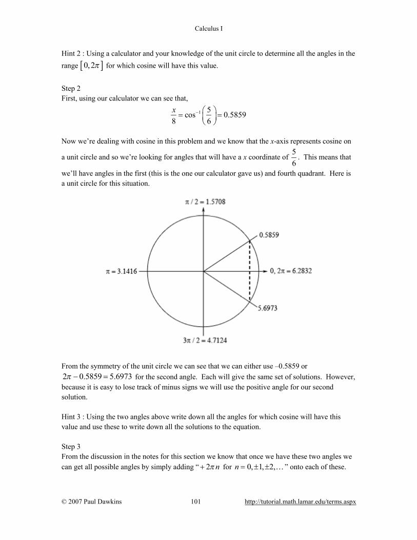
Calculus I
© 2007 Paul Dawkins 101 http://tutorial.math.lamar.edu/terms.aspx
Hint 2 : Using a calculator and your knowledge of the unit circle to determine all the angles in the range [ ]0,2π for which cosine will have this value.
Step 2 First, using our calculator we can see that,
1 5cos 0.58598 6x − = =
Now we’re dealing with cosine in this problem and we know that the x-axis represents cosine on
a unit circle and so we’re looking for angles that will have a x coordinate of 56
. This means that
we’ll have angles in the first (this is the one our calculator gave us) and fourth quadrant. Here is a unit circle for this situation.
From the symmetry of the unit circle we can see that we can either use –0.5859 or 2 0.5859 5.6973π − = for the second angle. Each will give the same set of solutions. However, because it is easy to lose track of minus signs we will use the positive angle for our second solution. Hint 3 : Using the two angles above write down all the angles for which cosine will have this value and use these to write down all the solutions to the equation. Step 3 From the discussion in the notes for this section we know that once we have these two angles we can get all possible angles by simply adding “ 2 nπ+ for 0, 1, 2,n = ± ± … ” onto each of these.
Calculus I
© 2007 Paul Dawkins 102 http://tutorial.math.lamar.edu/terms.aspx
This then means that we must have,
0.5859 2 OR 5.6973 2 0, 1, 2,8 8x xn n nπ π= + = + = ± ± …
Finally, to get all the solutions to the equation all we need to do is multiply both sides by 8 and we’ll convert everything to decimals to help with the final step.
4.6872 16 OR 45.5784 16 0, 1, 2,4.6872 50.2655 OR 45.5784 50.2655 0, 1, 2,
x n x n nn n n
π π= + = + = ± ±= + = + = ± ±
……
Hint 4 : Now all we need to do is plug in values of n to determine which solutions will actually fall in the given interval. Step 4 Now let’s find all the solutions. First notice that, in this case, if we plug in negative values of n we will get negative solutions and these will not be in the interval and so there is no reason to even try these. So, let’s start at 0n = and see what we get.
0 : 4.6872 OR 45.57841: 54.9527 OR 95.8439
n x xn x x
= = == = =
Notice that with each increase in n we were really just adding another 50.2655 onto the previous results and by doing this to the results from the 1n = step we will get solutions that are outside of the interval and so there is no reason to even plug in 2n = . So, it looks like we have the four solutions to this equation in the given interval.
4.6872, 45.5784, 54.9527, 95.8439x =
Note that depending upon the amount of decimals you used here your answers may vary slightly from these due to round off error. Any differences should be slight and only appear around the 4th decimal place or so however.
12. Find the solution(s) to ( )4 1 3sec 23
t= + that are in [ ]4,6− . Use at least 4 decimal places in
your work. Hint 1 : Find all the solutions to the equation without regard to the given interval. The first step in this process is to isolate the secant (with a coefficient of one) on one side of the equation. Step 1 Isolating the secant (with a coefficient of one) on one side of the equation gives,

Calculus I
© 2007 Paul Dawkins 103 http://tutorial.math.lamar.edu/terms.aspx
( ) 1sec 29
t =
At this point we can stop. We know that sec 1 or sec 1θ θ≤ − ≤
This means that it is impossible for secant to ever be 19
and so there will be no solution to this
equation. Note that if you didn’t recall the restrictions on secant the next step would have been to convert this to cosine so let’s do that.
( ) ( ) ( )1 1sec 2 cos 2 9cos 2 9
t tt
= = ⇒ =
At this point we can note that 1 cos 1θ− ≤ ≤ and so again there is no way for cosine to be 9 and again we get that there will be no solution to this equation.
Review : Solving Trig Equations with Calculators, Part II 1. Find all the solutions to ( )3 14sin 12 7 13t− + = . Use at least 4 decimal places in your work.
Hint : With the exception of the argument, which is a little more complex, this is identical to the equations that we solved in the previous section. Solution The argument of the sine is a little more complex in this equation than those we saw in the previous section, but the solution process is identical. Therefore, we will be assuming that you recall the process from the previous section and do not need all the hints or quite as many details as we put into the solutions there. If you are unsure of the process you should go back to the previous section and work some of the problems there before proceeding with the section. First, isolating the sine on one side of the equation gives,
( ) 5sin 12 77
t + = −
Using a calculator we get,
Calculus I
© 2007 Paul Dawkins 104 http://tutorial.math.lamar.edu/terms.aspx
1 512 7 sin 0.79567
t − + = − = −
From our knowledge of the unit circle we can see that a positive angle that corresponds to this angle is 2 0.7956 5.4876π − = . Either these angles can be used here but we’ll use the positive angle to avoid the possibility of losing the minus sign. Also, from a quick look at a unit circle we can see that a second angle in the range [ ]0, 2π will be 0.7965 3.9372π + = .
Now, all possible angles for which sine will have this value are, 12 7 3.9372 2 OR 12 7 5.4876 2 0, 1, 2,t n t n nπ π+ = + + = + = ± ± … At this point all we need to do is solve each of these for t and we’ll have all the solutions to the equation. Doing this gives,
0.2552 OR 0.1260 0, 1, 2,6 6n nt t nπ π
= − + = − + = ± ± …
If an interval had been given we would next proceed with plugging in values of n to determine which solutions fall in that interval. Since we were not given an interval this is as far as we can go. Note that depending upon the amount of decimals you used here your answers may vary slightly from these due to round off error. Any differences should be slight and only appear around the 4th decimal place or so however. 2. Find all the solutions to ( )3sec 4 9 24 0z− − = . Use at least 4 decimal places in your work.
Hint : With the exception of the argument, which is a little more complex, this is identical to the equations that we solved in the previous section. Solution The argument of the secant is a little more complex in this equation than those we saw in the previous section, but the solution process is identical. Therefore, we will be assuming that you recall the process from the previous section and do not need all the hints or quite as many details as we put into the solutions there. If you are unsure of the process you should go back to the previous section and work some of the problems there before proceeding with the section. First, isolating the secant on one side of the equation gives and converting the equation into one involving cosine (to make the work a little easier) gives,
( ) ( ) 1sec 4 9 8 cos 4 98
z z− = ⇒ − =

Calculus I
© 2007 Paul Dawkins 105 http://tutorial.math.lamar.edu/terms.aspx
Using a calculator we get,
1 14 9 cos 1.44558
z − − = =
From a quick look at a unit circle we can see that a second angle in the range [ ]0, 2π will be
2 1.4455 4.8377π − = . Now, all possible angles for which secant will have this value are, 4 9 1.4455 2 OR 4 9 4.8377 2 0, 1, 2,z n z n nπ π− = + − = + = ± ± … At this point all we need to do is solve each of these for z and we’ll have all the solutions to the equation. Doing this gives,
2 20.2838 OR 0.09308 0, 1, 2,9 9
n nz z nπ π= − = − − = ± ± …
If an interval had been given we would next proceed with plugging in values of n to determine which solutions fall in that interval. Since we were not given an interval this is as far as we can go. Note that depending upon the amount of decimals you used here your answers may vary slightly from these due to round off error. Any differences should be slight and only appear around the 4th decimal place or so however. 3. Find all the solutions to ( ) ( ) ( )4sin 2 15sin 2 tan 4 0x x x+ − + = . Use at least 4 decimal
places in your work. Hint 1 : Factor the equation and using basic algebraic properties get two equations that can be dealt with using known techniques. Step 1 Notice that each term has a sine in it and so we can factor this out of each term to get, ( ) ( )( )sin 2 4 15tan 4 0x x+ − = Now, we have a product of two factors that equals zero and so by basic algebraic properties we know that we must have, ( ) ( )sin 2 0 OR 4 15tan 4 0x x+ = − = Hint 2 : Solve each of these two equations to attain all the solutions to the original equation. Step 2
Calculus I
© 2007 Paul Dawkins 106 http://tutorial.math.lamar.edu/terms.aspx
Each of these equations are similar to equations solved in the previous section or in the earlier problems of this section. Therefore, we will be assuming that you can recall the solution process for each and we will not be putting in as many details. If you are unsure of the process you should go back to the previous section and work some of the problems there before proceeding with the solution to this problem. We’ll start with, ( )sin 2 0x + = From a unit circle we can see that we must have, 2 0 2 OR 2 2 0, 1, 2,x n x n nπ π π+ = + + = + = ± ± … Notice that we can further reduce this down to, 2 0, 1, 2,x n nπ+ = = ± ± … Finally, the solutions from this equation are, 2 0, 1, 2,x n nπ= − = ± ± … The second equation will take a little more (but not much more) work. First, isolating the tangent gives,
( ) 4tan 415
x =
Using our calculator we get,
1 44 tan 0.260615
x − = =
From our knowledge on solving equations involving tangents we know that the second angle in the range [ ]0, 2π will be 0.2606 3.4022π + = .
Finally, the solutions to this equation are,
4 0.2606 2 OR 4 3.4022 2 0, 1, 2,
0.06515 OR 0.8506 0, 1, 2,2 2
x n x n nn nx x n
π ππ π
= + = + = ± ±
= + = + = ± ±
…
…
Putting all of this together gives the following set of solutions.
2, 0.06515 , OR 0.8506 0, 1, 2,2 2n nx n x x nπ π
π= − = + = + = ± ± …
If an interval had been given we would next proceed with plugging in values of n to determine which solutions fall in that interval. Since we were not given an interval this is as far as we can go.

Calculus I
© 2007 Paul Dawkins 107 http://tutorial.math.lamar.edu/terms.aspx
Note that depending upon the amount of decimals you used here your answers may vary slightly from these due to round off error. Any differences should be slight and only appear around the 4th decimal place or so however.
4. Find all the solutions to 3 33cos sin 14cos 07 2 7y y y + =
. Use at least 4 decimal places
in your work. Hint 1 : Factor the equation and using basic algebraic properties get two equations that can be dealt with using known techniques. Step 1 Notice that each term has a cosine in it and so we can factor this out of each term to get,
3cos 3sin 14 07 2y y + =
Now, we have a product of two factors that equals zero and so by basic algebraic properties we know that we must have,
3cos 0 OR 3sin 14 07 2y y = + =
Hint 2 : Solve each of these two equations to attain all the solutions to the original equation. Step 2 Each of these equations are similar to equations solved in the previous section. Therefore, we will be assuming that you can recall the solution process for each and we will not be putting in as many details. If you are unsure of the process you should go back to the previous section and work some of the problems there before proceeding with the solution to this problem. We’ll start with,
3cos 07y =
From a unit circle we can see that we must have,
3 3 32 OR 2 0, 1, 2,7 2 7 2y yn n nπ π
π π= + = + = ± ± …
Notice that we can further reduce this down to,

Calculus I
© 2007 Paul Dawkins 108 http://tutorial.math.lamar.edu/terms.aspx
3 0, 1, 2,7 2y n nπ
π= + = ± ± …
Finally, the solutions from this equation are,
7 7 0, 1, 2,6 3
ny nπ π= + = ± ± …
The second equation will take a little more (but not much more) work. First, isolating the sine gives,
14sin 12 3y = − < −
At this point recall that we know 1 sin 1θ− ≤ ≤ and so this equation will have no solutions. Therefore, the only solutions to this equation are,
7 7 0, 1, 2,6 3
ny nπ π= + = ± ± …
Do get too excited about the fact that we only got solutions from one of the two equations we got after factoring. This will happen on occasion and so we need to be ready for these cases when they happen. If an interval had been given we would next proceed with plugging in values of n to determine which solutions fall in that interval. Since we were not given an interval this is as far as we can go. Note that depending upon the amount of decimals you used here your answers may vary slightly from these due to round off error. Any differences should be slight and only appear around the 4th decimal place or so however. 5. Find all the solutions to ( ) ( )27cos 3 cos 3 0x x− = . Use at least 4 decimal places in your
work. Hint 1 : Factor the equation and using basic algebraic properties get two equations that can be dealt with using known techniques. Step 1 Notice that we can factor a cosine out of each term to get, ( ) ( )( )cos 3 7cos 3 1 0x x − =

Calculus I
© 2007 Paul Dawkins 109 http://tutorial.math.lamar.edu/terms.aspx
Now, we have a product of two factors that equals zero and so by basic algebraic properties we know that we must have, ( ) ( )cos 3 0 OR 7cos 3 1 0x x= − = Hint 2 : Solve each of these two equations to attain all the solutions to the original equation. Step 2 Each of these equations are similar to equations solved in the previous section. Therefore, we will be assuming that you can recall the solution process for each and we will not be putting in as many details. If you are unsure of the process you should go back to the previous section and work some of the problems there before proceeding with the solution to this problem. We’ll start with, ( )cos 3 0x = From a unit circle we can see that we must have,
33 2 OR 3 2 0, 1, 2,2 2
x n x n nπ ππ π= + = + = ± ± …
Notice that we can further reduce this down to,
3 0, 1, 2,2
x n nππ= + = ± ± …
Finally, the solutions from this equation are,
0, 1, 2,6 3
nx nπ π= + = ± ± …
The second equation will take a little more (but not much more) work. First, isolating the cosine gives,
( ) 1cos 37
x =
Using our calculator we get,
1 13 cos 1.42747
x − = =
From a quick look at a unit circle we know that the second angle in the range [ ]0, 2π will be
2 1.4274 4.8558π − = . Finally, the solutions to this equation are,

Calculus I
© 2007 Paul Dawkins 110 http://tutorial.math.lamar.edu/terms.aspx
3 1.4274 2 OR 3 4.8558 2 0, 1, 2,
0.4758 OR 1.6186 0, 1, 2,3 3
x n x n nn nx x n
π ππ π
= + = + = ± ±
= + = + = ± ±
…
…
Putting all of this together gives the following set of solutions.
, 0.4758 , OR 1.6186 0, 1, 2,6 3 3 3
n n nx x x nπ π π π= + = + = + = ± ± …
If an interval had been given we would next proceed with plugging in values of n to determine which solutions fall in that interval. Since we were not given an interval this is as far as we can go. Note that depending upon the amount of decimals you used here your answers may vary slightly from these due to round off error. Any differences should be slight and only appear around the 4th decimal place or so however.
6. Find all the solutions to 2tan tan 124 4w w = +
. Use at least 4 decimal places in your
work. Hint 1 : Factor the equation and using basic algebraic properties get two equations that can be dealt with using known techniques. If you’re not sure how to factor this think about how you would factor 2 12 0x x− − = . Step 1 This equation may look very different from anything that we’ve ever been asked to factor, however it is something that we can factor. First think about factoring the following,
( ) ( )2 212 12 4 3 0x x x x x x= + → − − = − + =
If we can factor this algebraic equation then we can factor the given equation in exactly the same manner.
2
2
tan tan 124 4
tan tan 12 04 4
tan 4 tan 3 04 4
w w
w w
w w
= +
− − =
− + =
Calculus I
© 2007 Paul Dawkins 111 http://tutorial.math.lamar.edu/terms.aspx
Now, we have a product of two factors that equals zero and so by basic algebraic properties we know that we must have,
tan 4 0 OR tan 3 04 4w w − = + =
Hint 2 : Solve each of these two equations to attain all the solutions to the original equation. Step 2 Each of these equations are similar to equations solved in the previous section. Therefore, we will be assuming that you can recall the solution process for each and we will not be putting in as many details. If you are unsure of the process you should go back to the previous section and work some of the problems there before proceeding with the solution to this problem. We’ll start with the first equation and isolate the tangent to get,
tan 44w =
Using our calculator we get,
( )1tan 4 1.32584w −= =
From our knowledge on solving equations involving tangents we know that the second angle in the range [ ]0, 2π will be 1.3258 4.4674π + = .
All the solutions to the first equation are then,
1.3258 2 OR 4.4674 2 0, 1, 2,
4 45.3032 8 OR 17.8696 8 0, 1, 2,
w wn n n
w n w n n
π π
π π
= + = + = ± ±
= + = + = ± ±
…
…
Now, let’s solve the second equation.
( )1tan 3 tan 3 1.24904 4w w − = − → = − = −
From our knowledge of the unit circle we can see that a positive angle that corresponds to this angle is 2 1.2490 5.0342π − = . Either these angles can be used here but we’ll use the positive angle to avoid the possibility of losing the minus sign. Also, the second angle in the range
[ ]0, 2π is ( )1.2490 1.8926π + − = .
All the solutions to the second equation are then,
Calculus I
© 2007 Paul Dawkins 112 http://tutorial.math.lamar.edu/terms.aspx
1.8926 2 OR 5.0342 2 0, 1, 2,
4 47.5704 8 OR 20.1368 8 0, 1, 2,
w wn n n
w n w n n
π π
π π
= + = + = ± ±
= + = + = ± ±
…
…
Putting all of this together gives the following set of solutions.
5.3032 8 , 7.5704 8 ,
0, 1, 2,17.8696 8 , 20.1368 8
w n w nn
w n w nπ ππ π
= + = += ± ±
= + = +…
If an interval had been given we would next proceed with plugging in values of n to determine which solutions fall in that interval. Since we were not given an interval this is as far as we can go. Note that depending upon the amount of decimals you used here your answers may vary slightly from these due to round off error. Any differences should be slight and only appear around the 4th decimal place or so however. 7. Find all the solutions to ( ) ( )24csc 1 6 25csc 1t t− + = − . Use at least 4 decimal places in
your work. Hint 1 : Factor the equation and using basic algebraic properties get two equations that can be dealt with using known techniques. If you’re not sure how to factor this think about how you would factor 24 25 6 0x x− + = . Step 1 This equation may look very different from anything that we’ve ever been asked to factor, however it is something that we can factor. First think about factoring the following,
( ) ( )2 24 6 25 4 25 6 4 1 6 0x x x x x x+ = → − + = − − =
If we can factor this algebraic equation then we can factor the given equation in exactly the same manner.
( ) ( )( ) ( )
( )( ) ( )( )
2
2
4csc 1 6 25csc 1
4csc 1 25csc 1 6 0
4csc 1 1 csc 1 6 0
t t
t t
t t
− + = −
− − − + =
− − − − =
Now, we have a product of two factors that equals zero and so by basic algebraic properties we know that we must have, ( ) ( )4csc 1 1 0 OR csc 1 6 0t t− − = − − =

Calculus I
© 2007 Paul Dawkins 113 http://tutorial.math.lamar.edu/terms.aspx
Hint 2 : Solve each of these two equations to attain all the solutions to the original equation. Step 2 Each of these equations are similar to equations solved in the previous section and earlier in this section. Therefore, we will be assuming that you can recall the solution process for each and we will not be putting in as many details. If you are unsure of the process you should go back to the previous section and work some of the problems there before proceeding with the solution to this problem. We’ll start with the first equation, isolate the cosecant and convert to an equation in terms of sine for easier solving. Doing this gives,
( ) ( )1csc 1 sin 1 4 14
t t− = → − = >
We now know that there are now solutions to the first equation because we know 1 sin 1θ− ≤ ≤ . Now, let’s solve the second equation.
( ) ( ) 1csc 1 6 sin 16
t t− = → − =
Using our calculator we get,
1 11 sin 0.16746
t − − = =
A quick glance at a unit circle shows us that the second angle in the range [ ]0, 2π is
0.1674 2.9742π − = . All the solutions to the second equation are then,
1 0.1674 2 OR 1 2.9742 2 0, 1, 2,
0.8326 2 OR 1.9742 2 0, 1, 2,t n t n nt n t n n
π ππ π
− = + − = + = ± ±= − = − − = ± ±
……
Because we had not solutions to the first equation all the solutions to the original equation are then,
0.8326 2 OR 1.9742 2 0, 1, 2,t n t n nπ π= − = − − = ± ± … Do get too excited about the fact that we only got solutions from one of the two equations we got after factoring. This will happen on occasion and so we need to be ready for these cases when they happen. If an interval had been given we would next proceed with plugging in values of n to determine which solutions fall in that interval. Since we were not given an interval this is as far as we can go.
Calculus I
© 2007 Paul Dawkins 114 http://tutorial.math.lamar.edu/terms.aspx
Note that depending upon the amount of decimals you used here your answers may vary slightly from these due to round off error. Any differences should be slight and only appear around the 4th decimal place or so however. 8. Find all the solutions to ( )4 sec 7 21y y y= − . Use at least 4 decimal places in your work.
Hint 1 : Factor the equation and using basic algebraic properties get two equations that can be dealt with using known techniques. Step 1 Notice that if we move all the terms to one side we can then factor a y out of the equation. Doing this gives,
( )( )( )
4 sec 7 21 0
4sec 7 21 0
y y y
y y
+ =
+ =
Now, we have a product of two factors that equals zero and so by basic algebraic properties we know that we must have, ( )0 OR 4sec 7 21 0y y= + = Be careful with this type of equation to not make the mistake of just canceling the y from both sides in the initial step. Had you done that you would have missed the 0y = solution. When solving equations it is important to remember that you can’t cancel anything from both sides unless you know for a fact that what you are canceling will never be zero. Hint 2 : Solve each of these two equations to attain all the solutions to the original equation. Step 2 There really isn’t anything that we need to do with the first equation and so we can move right on to the second equation. Note that this equation is similar to equations solved in the previous section. Therefore, we will be assuming that you can recall the solution process for each and we will not be putting in as many details. If you are unsure of the process you should go back to the previous section and work some of the problems there before proceeding with the solution to this problem. First, isolating the secant and converting to cosines (to make the solving a little easier) gives,
( ) ( )21 4sec 7 cos 74 21
y y= − → = −
Calculus I
© 2007 Paul Dawkins 115 http://tutorial.math.lamar.edu/terms.aspx
Using our calculator we get,
1 47 cos 1.762421
y − = − =
From a quick look at a unit circle we know that the second angle in the range [ ]0, 2π will be
2 1.7624 4.5208π − = . Finally, the solutions to this equation are,
7 1.7624 2 OR 7 4.5208 2 0, 1, 2,
2 20.2518 OR 0.6458 0, 1, 2,7 7
y n y n nn ny y n
π ππ π
= + = + = ± ±
= + = + = ± ±
…
…
Putting all of this together gives the following set of solutions.
2 20, 0.2518 , OR 0.6458 0, 1, 2,7 7
n ny y y nπ π= = + = + = ± ± …
If an interval had been given we would next proceed with plugging in values of n to determine which solutions fall in that interval. Since we were not given an interval this is as far as we can go. Note that depending upon the amount of decimals you used here your answers may vary slightly from these due to round off error. Any differences should be slight and only appear around the 4th decimal place or so however. 9. Find all the solutions to ( ) ( )210 sin 3 2 7 sin 3 2x x x x+ = + . Use at least 4 decimal places in
your work. Hint 1 : Factor the equation and using basic algebraic properties get some equations that can be dealt with using known techniques. Step 1 Notice that if we move all the terms to one side we can then factor an x and a sine out of the equation. Doing this gives,
( ) ( )
( ) ( )
210 sin 3 2 7 sin 3 2 0
10 7 sin 3 2 0
x x x x
x x x
+ − + =
− + =
Now, we have a product of three factors that equals zero and so by basic algebraic properties we know that we must have,
Calculus I
© 2007 Paul Dawkins 116 http://tutorial.math.lamar.edu/terms.aspx
( )0, 10 7 0, OR sin 3 2 0x x x= − = + = Be careful with this type of equation to not make the mistake of just canceling the x or the sine from both sides in the initial step. Had you done that you would have missed the 0x = solution
and the solutions we will get from solving ( )sin 3 2 0x + = .
When solving equations it is important to remember that you can’t cancel anything from both sides unless you know for a fact that what you are canceling will never be zero. Hint 2 : Solve each of these three equations to attain all the solutions to the original equation. Step 2 There really isn’t anything that we need to do with the first equation and so we can move right on to the second equation (which also doesn’t really present any problems). Solving the second equation gives,
710
x =
Now let’s take a look at the third equation. This equation is similar to equations solved earlier in this section. Therefore, we will be assuming that you can recall the solution process for each and we will not be putting in as many details. If you are unsure of the process you should go back to the previous section and work some of the problems there before proceeding with the solution to this problem. From a unit circle we can see that we must have, 3 2 0 2 OR 3 2 2 0, 1, 2,x n x n nπ π π+ = + + = + = ± ± … Notice that we can further reduce this down to, 3 2 0, 1, 2,x n nπ+ = = ± ± … Finally, the solutions from this equation are,
2 0, 1, 2,3
nx nπ −= = ± ± …
Putting all of this together gives the following set of solutions.
7 20, , OR 0, 1, 2,10 3
nx x x nπ −= = = = ± ± …
If an interval had been given we would next proceed with plugging in values of n to determine which solutions fall in that interval. Since we were not given an interval this is as far as we can go.
Calculus I
© 2007 Paul Dawkins 117 http://tutorial.math.lamar.edu/terms.aspx
Note that depending upon the amount of decimals you used here your answers may vary slightly from these due to round off error. Any differences should be slight and only appear around the 4th decimal place or so however.
10. Find all the solutions to ( ) 62 3 tan 15 1011
tt t − = −
. Use at least 4 decimal places in your
work. Hint 1 : Factor the equation and using basic algebraic properties get two equations that can be dealt with using known techniques. Step 1 This one may be a little trickier to factor than the others in this section, but it can be factored. First get everything on one side of the equation and then notice that we can factor out a 2 3t − from the equation as follows,
( )
( ) ( )
( )
62 3 tan 10 15 011
62 3 tan 5 2 3 011
62 3 tan 5 011
tt t
tt t
tt
− + − =
− + − =
− + =
Now, we have a product of two factors that equals zero and so by basic algebraic properties we know that we must have,
62 3 0 OR tan 5 011
tt − = + =
Be careful with this type of equation to not make the mistake of just canceling the 2 3t − from both sides. Had you done that you would have missed the solution from the first equation. When solving equations it is important to remember that you can’t cancel anything from both sides unless you know for a fact that what you are canceling will never be zero. Hint 2 : Solve each of these two equations to attain all the solutions to the original equation. Step 2 Solving the first equation gives,
32
t =
Calculus I
© 2007 Paul Dawkins 118 http://tutorial.math.lamar.edu/terms.aspx
Now we can move onto the second equation and note that this equation is similar to equations solved in the previous section. Therefore, we will be assuming that you can recall the solution process for each and we will not be putting in as many details. If you are unsure of the process you should go back to the previous section and work some of the problems there before proceeding with the solution to this problem. First, isolating the tangent gives,
6tan 511
t = −
Using our calculator we get,
( )16 tan 5 1.373411
t −= − = −
From our knowledge of the unit circle we can see that a positive angle that corresponds to this angle is 2 1.3734 4.9098π − = . Either these angles can be used here but we’ll use the positive angle to avoid the possibility of losing the minus sign. Also, the second angle in the range
[ ]0, 2π is ( )1.3734 1.7682π + − = .
Finally, the solutions to this equation are,
6 61.7682 2 OR 4.9098 2 0, 1, 2,11 11
11 113.2417 OR 9.0013 0, 1, 2,3 3
t tn n n
n nt t n
π π
π π
= + = + = ± ±
= + = + = ± ±
…
…
Putting all of this together gives the following set of solutions.
3 11 11, 3.2417 , OR 9.0013 0, 1, 2,2 3 3
n nt t t nπ π= = + = + = ± ± …
If an interval had been given we would next proceed with plugging in values of n to determine which solutions fall in that interval. Since we were not given an interval this is as far as we can go. Note that depending upon the amount of decimals you used here your answers may vary slightly from these due to round off error. Any differences should be slight and only appear around the 4th decimal place or so however.
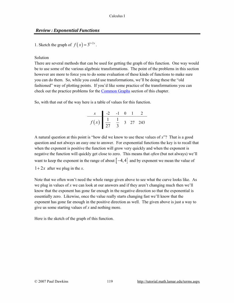
Calculus I
© 2007 Paul Dawkins 119 http://tutorial.math.lamar.edu/terms.aspx
Review : Exponential Functions 1. Sketch the graph of ( ) 1 23 xf x += .
Solution There are several methods that can be used for getting the graph of this function. One way would be to use some of the various algebraic transformations. The point of the problems in this section however are more to force you to do some evaluation of these kinds of functions to make sure you can do them. So, while you could use transformations, we’ll be doing these the “old fashioned” way of plotting points. If you’d like some practice of the transformations you can check out the practice problems for the Common Graphs section of this chapter. So, with that out of the way here is a table of values for this function.
x -2 -1 0 1 2
( )f x 127
13
3 27 243
A natural question at this point is “how did we know to use these values of x”? That is a good question and not always an easy one to answer. For exponential functions the key is to recall that when the exponent is positive the function will grow very quickly and when the exponent is negative the function will quickly get close to zero. This means that often (but not always) we’ll want to keep the exponent in the range of about [ ]4,4− and by exponent we mean the value of
1 2x+ after we plug in the x. Note that we often won’t need the whole range given above to see what the curve looks like. As we plug in values of x we can look at our answers and if they aren’t changing much then we’ll know that the exponent has gone far enough in the negative direction so that the exponential is essentially zero. Likewise, once the value really starts changing fast we’ll know that the exponent has gone far enough in the positive direction as well. The given above is just a way to give us some starting values of x and nothing more. Here is the sketch of the graph of this function.
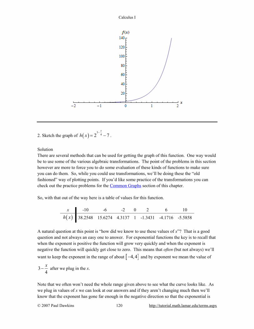
Calculus I
© 2007 Paul Dawkins 120 http://tutorial.math.lamar.edu/terms.aspx
2. Sketch the graph of ( )3
42 7x
h x−
= − .
Solution There are several methods that can be used for getting the graph of this function. One way would be to use some of the various algebraic transformations. The point of the problems in this section however are more to force you to do some evaluation of these kinds of functions to make sure you can do them. So, while you could use transformations, we’ll be doing these the “old fashioned” way of plotting points. If you’d like some practice of the transformations you can check out the practice problems for the Common Graphs section of this chapter. So, with that out of the way here is a table of values for this function.
x -10 -6 -2 0 2 6 10
( )h x 38.2548 15.6274 4.3137 1 -1.3431 -4.1716 -5.5858
A natural question at this point is “how did we know to use these values of x”? That is a good question and not always an easy one to answer. For exponential functions the key is to recall that when the exponent is positive the function will grow very quickly and when the exponent is negative the function will quickly get close to zero. This means that often (but not always) we’ll want to keep the exponent in the range of about [ ]4,4− and by exponent we mean the value of
34x
− after we plug in the x.
Note that we often won’t need the whole range given above to see what the curve looks like. As we plug in values of x we can look at our answers and if they aren’t changing much then we’ll know that the exponent has gone far enough in the negative direction so that the exponential is

Calculus I
© 2007 Paul Dawkins 121 http://tutorial.math.lamar.edu/terms.aspx
essentially zero. Likewise, once the value really starts changing fast we’ll know that the exponent has gone far enough in the positive direction as well. The given above is just a way to give us some starting values of x and nothing more. Here is the sketch of the graph of this function.
3. Sketch the graph of ( ) 2 48 3 th t −= + e .
Solution There are several methods that can be used for getting the graph of this function. One way would be to use some of the various algebraic transformations. The point of the problems in this section however are more to force you to do some evaluation of these kinds of functions to make sure you can do them. So, while you could use transformations, we’ll be doing these the “old fashioned” way of plotting points. If you’d like some practice of the transformations you can check out the practice problems for the Common Graphs section of this chapter. So, with that out of the way here is a table of values for this function.
t -1 0 1 2 3
( )h t 8.0074 8.0549 8.4060 11 30.1672
A natural question at this point is “how did we know to use these values of t”? That is a good question and not always an easy one to answer. For exponential functions the key is to recall that when the exponent is positive the function will grow very quickly and when the exponent is negative the function will quickly get close to zero. This means that often (but not always) we’ll want to keep the exponent in the range of about [ ]4,4− and by exponent we mean the value of
2 4t − after we plug in the t.
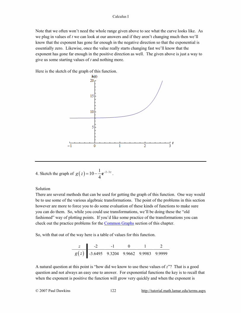
Calculus I
© 2007 Paul Dawkins 122 http://tutorial.math.lamar.edu/terms.aspx
Note that we often won’t need the whole range given above to see what the curve looks like. As we plug in values of t we can look at our answers and if they aren’t changing much then we’ll know that the exponent has gone far enough in the negative direction so that the exponential is essentially zero. Likewise, once the value really starts changing fast we’ll know that the exponent has gone far enough in the positive direction as well. The given above is just a way to give us some starting values of t and nothing more. Here is the sketch of the graph of this function.
4. Sketch the graph of ( ) 2 31104
zg z − −= − e .
Solution There are several methods that can be used for getting the graph of this function. One way would be to use some of the various algebraic transformations. The point of the problems in this section however are more to force you to do some evaluation of these kinds of functions to make sure you can do them. So, while you could use transformations, we’ll be doing these the “old fashioned” way of plotting points. If you’d like some practice of the transformations you can check out the practice problems for the Common Graphs section of this chapter. So, with that out of the way here is a table of values for this function.
z -2 -1 0 1 2
( )g z -3.6495 9.3204 9.9662 9.9983 9.9999
A natural question at this point is “how did we know to use these values of z”? That is a good question and not always an easy one to answer. For exponential functions the key is to recall that when the exponent is positive the function will grow very quickly and when the exponent is

Calculus I
© 2007 Paul Dawkins 123 http://tutorial.math.lamar.edu/terms.aspx
negative the function will quickly get close to zero. This means that often (but not always) we’ll want to keep the exponent in the range of about [ ]4,4− and by exponent we mean the value of
2 3z− − after we plug in the z. Note that we often won’t need the whole range given above to see what the curve looks like. As we plug in values of z we can look at our answers and if they aren’t changing much then we’ll know that the exponent has gone far enough in the negative direction so that the exponential is essentially zero. Likewise, once the value really starts changing fast we’ll know that the exponent has gone far enough in the positive direction as well. The given above is just a way to give us some starting values of z and nothing more. Here is the sketch of the graph of this function.
Review : Logarithm Functions 1. Without using a calculator determine the exact value of 3log 81 . Hint : Recall that converting a logarithm to exponential form can often help to evaluate these kinds of logarithms. Solution Converting the logarithm to exponential form gives, ?
3log 81 ? 3 81= ⇒ = From this we can quickly see that 43 81= and so we must have,
Calculus I
© 2007 Paul Dawkins 124 http://tutorial.math.lamar.edu/terms.aspx
3log 81 4= 2. Without using a calculator determine the exact value of 5log 125 . Hint : Recall that converting a logarithm to exponential form can often help to evaluate these kinds of logarithms. Solution Converting the logarithm to exponential form gives, ?
5log 125 ? 5 125= ⇒ = From this we can quickly see that 35 125= and so we must have,
5log 125 3=
3. Without using a calculator determine the exact value of 21log8
.
Hint : Recall that converting a logarithm to exponential form can often help to evaluate these kinds of logarithms. Solution Converting the logarithm to exponential form gives,
?2
1 1log ? 28 8
= ⇒ =
Now, we know that if we raise an integer to a negative exponent we’ll get a fraction and so we must have a negative exponent and then we know that 32 8= . Therefore we can see that
3 128
− = and so we must have,
21log 38
= −
4. Without using a calculator determine the exact value of 1
4
log 16 .

Calculus I
© 2007 Paul Dawkins 125 http://tutorial.math.lamar.edu/terms.aspx
Hint : Recall that converting a logarithm to exponential form can often help to evaluate these kinds of logarithms. Solution Converting the logarithm to exponential form gives,
?
14
1log 16 ? 164
= ⇒ =
Now, we know that if we raise an fraction to a power and get an integer out we must have had a negative exponent. Now, we also know that 24 16= . Therefore we can see that
2 21 4 164 1
− = =
and so we must have,
14
log 16 2= −
5. Without using a calculator determine the exact value of 4ln e . Hint : Recall that converting a logarithm to exponential form can often help to evaluate these kinds of logarithms. Also recall what the base is for a natural logarithm. Solution Recalling that the base for a natural logarithm is e and converting the logarithm to exponential form gives, 4 4 ? 4ln log ?= = ⇒ =ee e e e From this we can quickly see that 4 4=e e and so we must have,
4ln 4=e Note that an easier method of determining the value of this logarithm would have been to recall the properties of logarithm. In particular the property that states, log x
b b x= Using this we can also very quickly see what the value of the logarithm is.
6. Without using a calculator determine the exact value of 1log
100.
Calculus I
© 2007 Paul Dawkins 126 http://tutorial.math.lamar.edu/terms.aspx
Hint : Recall that converting a logarithm to exponential form can often help to evaluate these kinds of logarithms. Also recall what the base is for a common logarithm. Solution Recalling that the base for a natural logarithm is 10 and converting the logarithm to exponential form gives,
?10
1 1 1log log ? 10100 100 100
= = ⇒ =
Now, we know that if we raise an integer to a negative exponent we’ll get a fraction and so we must have a negative exponent and then we know that 210 100= . Therefore we can see that
2 110100
− = and so we must have,
1log 2100
= −
7. Write ( )4 7log 3x y− in terms of simpler logarithms.
Solution So, we’re being asked here to use as many of the properties as we can to reduce this down into simpler logarithms. So, here is the work for this problem.
( ) ( ) ( ) ( )
( ) ( ) ( )
4 7 4 7log 3 log 3 log log
log 3 4log 7 log
x y x y
x y
− −= + +
= + −
Remember that we can only bring an exponent out of a logarithm if is on the whole argument of the logarithm. In other words, we couldn’t bring any of the exponents out of the logarithms until we had dealt with the product.
8. Write ( )2 2ln x y z+ in terms of simpler logarithms.
Solution So, we’re being asked here to use as many of the properties as we can to reduce this down into simpler logarithms. So, here is the work for this problem.
Calculus I
© 2007 Paul Dawkins 127 http://tutorial.math.lamar.edu/terms.aspx
( ) ( ) ( )
( ) ( )
12 2 2 2 2
2 2
ln ln ln
1ln ln2
x y z x y z
x y z
+ = + +
= + +
Remember that we can only bring an exponent out of a logarithm if is on the whole argument of the logarithm. In other words, we couldn’t bring any of the exponents out of the logarithms until we had dealt with the product. Also, in the second logarithm while each term is squared the
whole argument is not squared, i.e. it’s not ( )2x y+ and so we can’t bring those 2’s out of the
logarithm.
9. Write 4 2 5
4log xy z
−
in terms of simpler logarithms.
Solution So, we’re being asked here to use as many of the properties as we can to reduce this down into simpler logarithms. So, here is the work for this problem.
( )
( ) ( )
( ) ( ) ( )
12 5
4 4 42 5
12 5
4 4 4
4 4 4
4log log 4 log
log 4 log log
1log 4 2log log5
x x y zy z
x y z
x y z
−= − −
= − − +
= − − −
Remember that we can only bring an exponent out of a logarithm if is on the whole argument of the logarithm. In other words, we couldn’t bring any of the exponents out of the logarithms until we had dealt with the quotient and product. Recall as well that we can’t split up an sum/difference in a logarithm. Finally, make sure that you are careful in dealing with the minus sign we get from breaking up the quotient when dealing with the product in the denominator.
10. Combine 4 4 412log 5log log2
x y z+ − into a single logarithm with a coefficient of one.
Hint :The properties that we use to break up logarithms can be used in reverse as well.
Calculus I
© 2007 Paul Dawkins 128 http://tutorial.math.lamar.edu/terms.aspx
Solution To convert this into a single logarithm we’ll be using the properties that we used to break up logarithms in reverse. The first step in this process is to use the property,
( )log logrb bx r x=
to make sure that all the logarithms have coefficients of one. This needs to be done first because all the properties that allow us to combine sums/differences of logarithms require coefficients of one on individual logarithms. So, using this property gives,
( ) ( )1
2 5 24 4 4log log logx y z
+ −
Now, there are several ways to proceed from this point. We can use either of the two properties.
( )log log log log log logb b b b b bxxy x y x yy
= + = −
and in fact we’ll need to use both in the end. Which we use first does not matter as we’ll end up with the same result in the end. Here is the rest of the work for this problem.
( ) ( )2 54 4 4 4 4
2 5
4
12log 5log log log log2
log
x y z x y z
x yz
+ − = −
=
Note that the only reason we converted the fractional exponent to a root was to make the final answer a little nicer. 11. Combine ( ) ( )3ln 5 4ln 2ln 1t t s+ − − − into a single logarithm with a coefficient of one.
Hint :The properties that we use to break up logarithms can be used in reverse as well. Solution To convert this into a single logarithm we’ll be using the properties that we used to break up logarithms in reverse. The first step in this process is to use the property,
( )log logrb bx r x=
to make sure that all the logarithms have coefficients of one. This needs to be done first because all the properties that allow us to combine sums/differences of logarithms require coefficients of one on individual logarithms. So, using this property gives,
( ) ( ) ( )3 24ln 5 ln ln 1t t s+ − − − Now, there are several ways to proceed from this point. We can use either of the two properties.

Calculus I
© 2007 Paul Dawkins 129 http://tutorial.math.lamar.edu/terms.aspx
( )log log log log log logb b b b b bxxy x y x yy
= + = −
and in fact we’ll need to use both in the end. We should also be careful with the fact that there are two minus signs in here as that sometimes adds confusion to the problem. They are easy to deal with however if we just factor a minus sign out of the last two terms and then proceed from there as follows.
( ) ( ) ( ) ( ) ( )( )
( ) ( )( ) ( )( )
3 24
33 24
24
3ln 5 4ln 2ln 1 ln 5 ln ln 1
5ln 5 ln 1 ln
1
t t s t t s
tt t s
t s
+ − − − = + − + −
+= + − − =
−
12. Combine 1 log 6 log 23
a b− + into a single logarithm with a coefficient of one.
Hint :The properties that we use to break up logarithms can be used in reverse as well. For the constant see if you figure out a way to write that as a logarithm. Solution To convert this into a single logarithm we’ll be using the properties that we used to break up logarithms in reverse. The first step in this process is to use the property,
( )log logrb bx r x=
to make sure that all the logarithms have coefficients of one. This needs to be done first because all the properties that allow us to combine sums/differences of logarithms require coefficients of one on individual logarithms. So, using this property gives,
( )1
63log log 2a b
− +
Now, for the 2 let’s notice that we can write this in terms of a logarithm as, 22 log10 log100= = Note that this is really just using the property, log x
b b x= So, we now have,
( )1
63log log log100a b
− +

Calculus I
© 2007 Paul Dawkins 130 http://tutorial.math.lamar.edu/terms.aspx
Now, there are several ways to proceed from this point. We can use either of the two properties.
( )log log log log log logb b b b b bxxy x y x yy
= + = −
and in fact we’ll need to use both in the end. Which we use first does not matter as we’ll end up with the same result in the end. Here is the rest of the work for this problem.
( ) ( ) ( )1
6 2 633
3
6
log log log10 log 100 log
100log
a b a b
ab
− + = −
=
Note that the only reason we converted the fractional exponent to a root was to make the final answer a little nicer. 13. Use the change of base formula and a calculator to find the value of 12log 35 . Solution We can use either the natural logarithm or the common logarithm to do this so we’ll do both.
12ln 35 3.55534806log 35 1.43077731ln12 2.48490665
= = =
12log35 1.54406804log 35 1.43077731log12 1.07918125
= = =
So, as we noted at the start it doesn’t matter which logarithm we use we’ll get the same answer in the end. 14. Use the change of base formula and a calculator to find the value of 2
3
log 53 .
Solution We can use either the natural logarithm or the common logarithm to do this so we’ll do both.
23
ln 53 3.97029191log 53 9.791944692 0.40546511ln3
= = = −−

Calculus I
© 2007 Paul Dawkins 131 http://tutorial.math.lamar.edu/terms.aspx
23
log 53 1.72427587log 53 9.791944692 0.17609126log3
= = = −−
So, as we noted at the start it doesn’t matter which logarithm we use we’ll get the same answer in the end.
Review : Exponential and Logarithm Equations 1. Find all the solutions to 7 312 4 7x+− =e . If there are no solutions clearly explain why. Step 1 There isn’t all that much to do here for this equation. First we need to isolate the exponential on one side by itself with a coefficient of one.
7 3 7 3 54 54
x x+ +− = − ⇒ =e e
Step 2 Now all we need to do is take the natural logarithm of both sides and then solve for x.
( )7 3 5ln ln457 3 ln4
1 5ln 7 2.258953 4
x
x
x
+ = + =
= − = −
e
Depending upon your preferences either the exact or decimal solution can be used.
2. Find all the solutions to 2 21 10 3 z z−= − e . If there are no solutions clearly explain why.
Step 1 There isn’t all that much to do here for this equation. First we need to isolate the exponential on one side by itself with a coefficient of one.
2 22 29 3 3z z z z− −− = − ⇒ =e e
Step 2 Now all we need to do is take the natural logarithm of both sides and then solve for z.
Calculus I
© 2007 Paul Dawkins 132 http://tutorial.math.lamar.edu/terms.aspx
( ) ( )
( )( )
2 2
2
2
ln ln 3
2 ln 3
2 ln 3 0
z z
z z
z z
− =
− =
− − =
e
Now, before proceeding with the solution here let’s pause and make sure that we don’t get too excited about the “strangeness” of the quadratic above. If we’d had the quadratic, 2 2 5 0z z− − = for instance, we’d know that all we would need to do is use the quadratic formula to get the solutions. That’s all we need to as well for the quadratic that we have from our work. Of course we don’t have a 5 we have a ln(3), but ln(3) is just a number and so we can use the quadratic formula to find the solutions here as well. Here is the work for that.
( ) ( ) ( ) ( )( )( )
( )
( )( ) ( ) ( )
22 2 4 1 ln 3 2 4 4ln 32 1 2
2 4 1 ln 3 2 2 1 ln 31 1 ln 3 0.4487, 2.4487
2 2
z− − ± − − − ± +
= =
± + ± += = = ± + = −
Notice that we did a little simplification on the root. This doesn’t need to be done, but can make the exact solution a little easier to deal with. Also, depending upon your preferences either the exact or decimal solution can be used. Before leaving this solution we should again make a point that not all quadratics will be the “simple” type of quadratics that you may be used to solving from an Algebra class. They can, and often will be, messier that those. That doesn’t mean that you can’t solve them. They are, for all intents and purposes, identical to the types of problems you are used to working. The only real difference is that they numbers are a little messier. So, don’t get too excited about this kind of problem. They will happen on occasion and you are capable of solving them! 3. Find all the solutions to 6 12 0tt t −− =e . If there are no solutions clearly explain why. Hint : Be careful to not cancel terms that shouldn’t be canceled. Remember that you can’t cancel something unless you know for a fact that it won’t ever be zero. Also, note that if you can cancel something then it can be factored out of the equation. Step 1 First notice that we can factor a t out of both terms to get,

Calculus I
© 2007 Paul Dawkins 133 http://tutorial.math.lamar.edu/terms.aspx
( )6 12 0tt −− =e Be careful to not cancel the t from both terms. When solving equations you can only cancel something if you know for a fact that it won’t be zero. If the term can be zero and you cancel it you will miss solutions and that will the case here. Step 2 We now have a product of terms that is equal to zero so we know, 6 10 OR 2 0tt −= − =e So, we have one solution already, 0t = , and again note that if we had canceled the t at the beginning we would have missed this solution. Now all we need to do is solve the equation involving the exponential. Step 3 We can now solve the exponential equation in the same manner as the first couple of problems in this section.
( ) ( )
( )
( )( )
6 1
6 1
2
ln ln 2
6 1 ln 2
1 1 ln 2 0.28226
t
t
t
t
−
−
=
=
− =
= + =
e
e
Depending upon your preferences either the exact or decimal solution can be used.
4. Find all the solutions to ( ) 2 24 1 12 3 xx x −+ = + e . If there are no solutions clearly explain why.
Hint : Be careful to not cancel terms that shouldn’t be canceled. Remember that you can’t cancel something unless you know for a fact that it won’t ever be zero. Also, note that if you can cancel something then it can be factored out of the equation. Step 1 It may not be apparent at first glance, but with some work we can do a little factoring on this equation. To do that first move everything to one side and then the factoring might become a little more apparent.
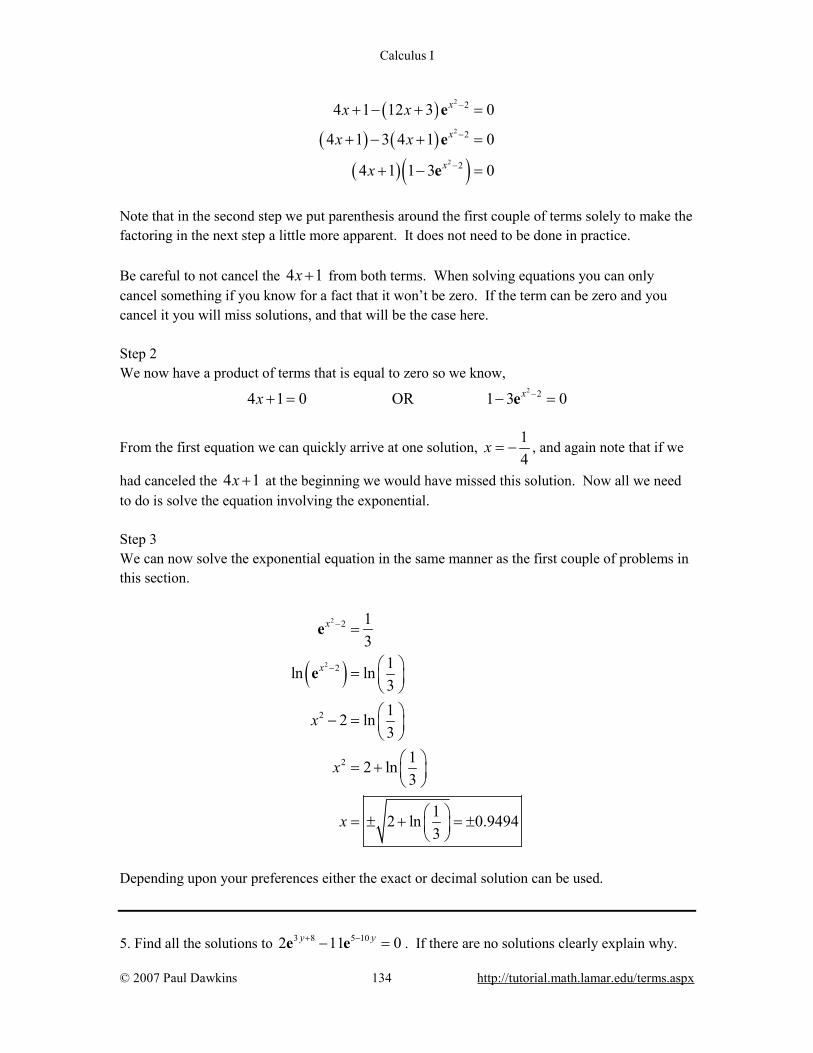
Calculus I
© 2007 Paul Dawkins 134 http://tutorial.math.lamar.edu/terms.aspx
( )( ) ( )
( )( )
2
2
2
2
2
2
4 1 12 3 0
4 1 3 4 1 0
4 1 1 3 0
x
x
x
x x
x x
x
−
−
−
+ − + =
+ − + =
+ − =
e
e
e
Note that in the second step we put parenthesis around the first couple of terms solely to make the factoring in the next step a little more apparent. It does not need to be done in practice. Be careful to not cancel the 4 1x + from both terms. When solving equations you can only cancel something if you know for a fact that it won’t be zero. If the term can be zero and you cancel it you will miss solutions, and that will be the case here. Step 2 We now have a product of terms that is equal to zero so we know,
2 24 1 0 OR 1 3 0xx −+ = − =e
From the first equation we can quickly arrive at one solution, 14
x = − , and again note that if we
had canceled the 4 1x + at the beginning we would have missed this solution. Now all we need to do is solve the equation involving the exponential. Step 3 We can now solve the exponential equation in the same manner as the first couple of problems in this section.
( )
2
2
2
2
2
2
13
1ln ln312 ln3
12 ln3
12 ln 0.94943
x
x
x
x
x
−
−
=
= − =
= +
= ± + = ±
e
e
Depending upon your preferences either the exact or decimal solution can be used. 5. Find all the solutions to 3 8 5 102 11 0y y+ −− =e e . If there are no solutions clearly explain why.
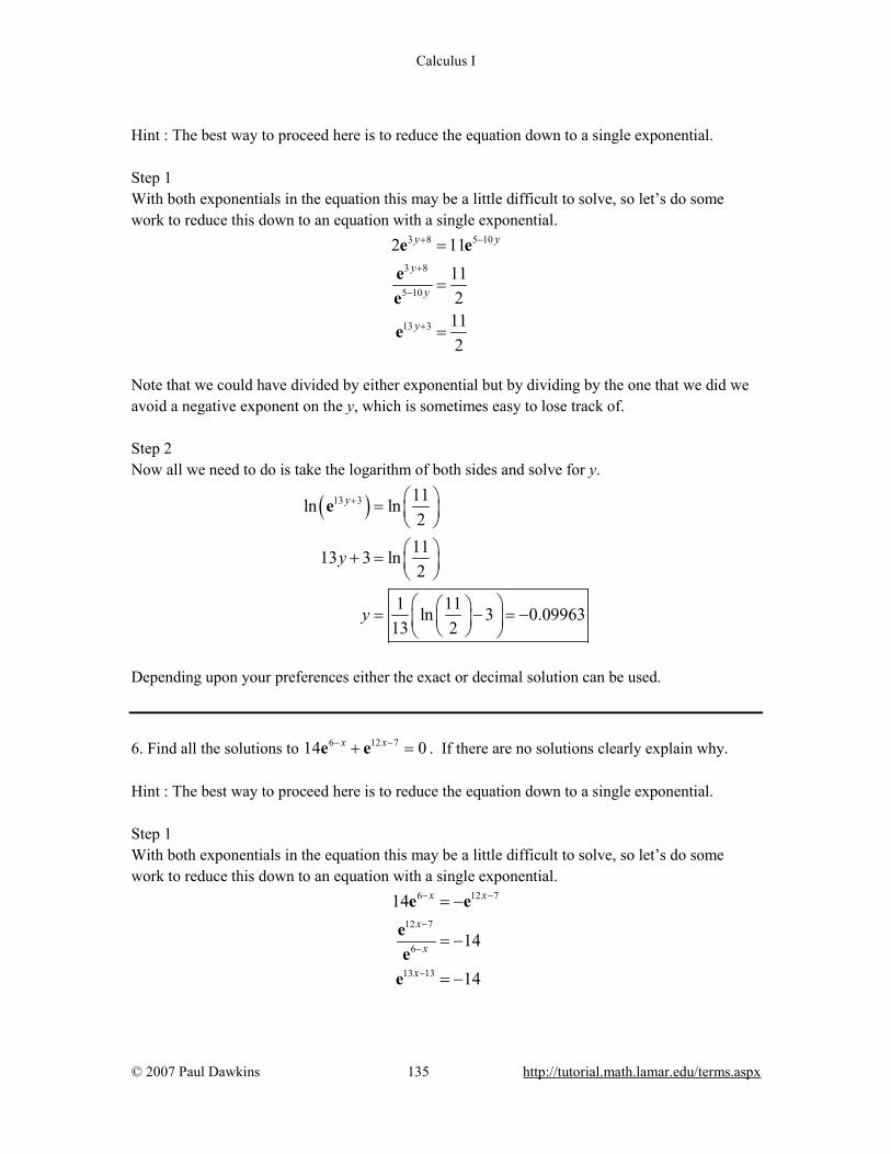
Calculus I
© 2007 Paul Dawkins 135 http://tutorial.math.lamar.edu/terms.aspx
Hint : The best way to proceed here is to reduce the equation down to a single exponential. Step 1 With both exponentials in the equation this may be a little difficult to solve, so let’s do some work to reduce this down to an equation with a single exponential.
3 8 5 10
3 8
5 10
13 3
2 11112
112
y y
y
y
y
+ −
+
−
+
=
=
=
e eee
e
Note that we could have divided by either exponential but by dividing by the one that we did we avoid a negative exponent on the y, which is sometimes easy to lose track of. Step 2 Now all we need to do is take the logarithm of both sides and solve for y.
( )13 3 11ln ln2
1113 3 ln2
1 11ln 3 0.0996313 2
y
y
y
+ = + =
= − = −
e
Depending upon your preferences either the exact or decimal solution can be used. 6. Find all the solutions to 6 12 714 0x x− −+ =e e . If there are no solutions clearly explain why. Hint : The best way to proceed here is to reduce the equation down to a single exponential. Step 1 With both exponentials in the equation this may be a little difficult to solve, so let’s do some work to reduce this down to an equation with a single exponential.
6 12 7
12 7
6
13 13
14
14
14
x x
x
x
x
− −
−
−
−
= −
= −
= −
e eee
e
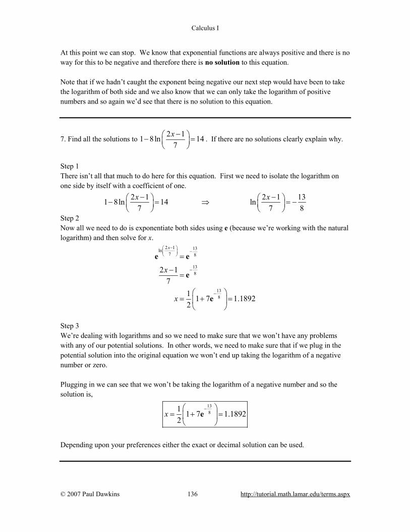
Calculus I
© 2007 Paul Dawkins 136 http://tutorial.math.lamar.edu/terms.aspx
At this point we can stop. We know that exponential functions are always positive and there is no way for this to be negative and therefore there is no solution to this equation. Note that if we hadn’t caught the exponent being negative our next step would have been to take the logarithm of both side and we also know that we can only take the logarithm of positive numbers and so again we’d see that there is no solution to this equation.
7. Find all the solutions to 2 11 8ln 14
7x − − =
. If there are no solutions clearly explain why.
Step 1 There isn’t all that much to do here for this equation. First we need to isolate the logarithm on one side by itself with a coefficient of one.
2 1 2 1 131 8ln 14 ln7 7 8
x x− − − = ⇒ = −
Step 2 Now all we need to do is exponentiate both sides using e (because we’re working with the natural logarithm) and then solve for x.
2 1 13ln7 8
138
138
2 17
1 1 7 1.18922
x
x
x
− −
−
−
=
−=
= + =
e e
e
e
Step 3 We’re dealing with logarithms and so we need to make sure that we won’t have any problems with any of our potential solutions. In other words, we need to make sure that if we plug in the potential solution into the original equation we won’t end up taking the logarithm of a negative number or zero. Plugging in we can see that we won’t be taking the logarithm of a negative number and so the solution is,
1381 1 7 1.1892
2x
− = + =
e
Depending upon your preferences either the exact or decimal solution can be used.
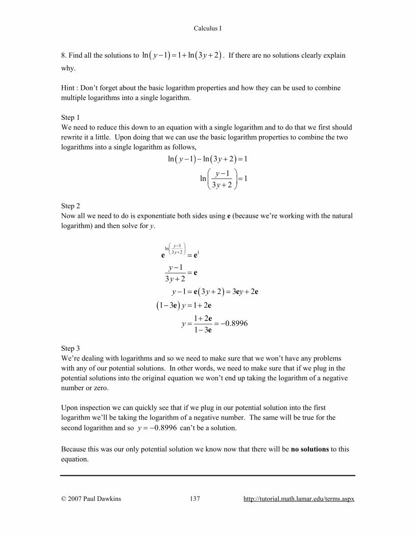
Calculus I
© 2007 Paul Dawkins 137 http://tutorial.math.lamar.edu/terms.aspx
8. Find all the solutions to ( ) ( )ln 1 1 ln 3 2y y− = + + . If there are no solutions clearly explain
why. Hint : Don’t forget about the basic logarithm properties and how they can be used to combine multiple logarithms into a single logarithm. Step 1 We need to reduce this down to an equation with a single logarithm and to do that we first should rewrite it a little. Upon doing that we can use the basic logarithm properties to combine the two logarithms into a single logarithm as follows,
( ) ( )ln 1 ln 3 2 1
1ln 13 2
y y
yy
− − + =
−= +
Step 2 Now all we need to do is exponentiate both sides using e (because we’re working with the natural logarithm) and then solve for y.
( )( )
1ln3 2 1
13 2
1 3 2 3 2
1 3 1 21 2 0.89961 3
yy
yyy y y
y
y
− + =
−=
+
− = + = +
− = +
+= = −
−
e e
e
e e e
e eee
Step 3 We’re dealing with logarithms and so we need to make sure that we won’t have any problems with any of our potential solutions. In other words, we need to make sure that if we plug in the potential solutions into the original equation we won’t end up taking the logarithm of a negative number or zero. Upon inspection we can quickly see that if we plug in our potential solution into the first logarithm we’ll be taking the logarithm of a negative number. The same will be true for the second logarithm and so 0.8996y = − can’t be a solution. Because this was our only potential solution we know now that there will be no solutions to this equation.

Calculus I
© 2007 Paul Dawkins 138 http://tutorial.math.lamar.edu/terms.aspx
9. Find all the solutions to ( ) ( )log log 21 2w w+ − = . If there are no solutions clearly explain
why. Hint : Don’t forget about the basic logarithm properties and how they can be used to combine multiple logarithms into a single logarithm. Step 1 We need to reduce this down to an equation with a single logarithm and to do that we first should rewrite it a little. Upon doing that we can use the basic logarithm properties to combine the two logarithms into a single logarithm as follows,
( )( )
( )2
log 21 2
log 21 2
w w
w w
− =
− =
Step 2 Now all we need to do is exponentiate both sides using 10 (because we’re working with the common logarithm) and then solve for y.
( )( )
( ) ( )
2
2
log 21 2
2
2
log 21 2
10 1021 100
21 100 025 4 0 4, 25
w w
w w
ww
w w w w
−
− =
=
− =
− − =
− + = ⇒ = − =
Step 3 We’re dealing with logarithms and so we need to make sure that we won’t have any problems with any of our potential solutions. In other words, we need to make sure that if we plug either of the two potential solutions into the original equation we won’t end up taking the logarithm of a negative number or zero. Upon inspection we can quickly see that if we plug in 4w = − we will be taking a logarithm of a negative number (in both of the logarithms in this case) and so 4w = − can’t be a solution. On the other hand, if we plug in 25w = we won’t be taking logarithms of negative numbers and so
25w = is a solution.
In summary then, the only solution to the equation is : 25w = . 10. Find all the solutions to ( ) ( )2log log 7 1 0z z− − = . If there are no solutions clearly explain
why.
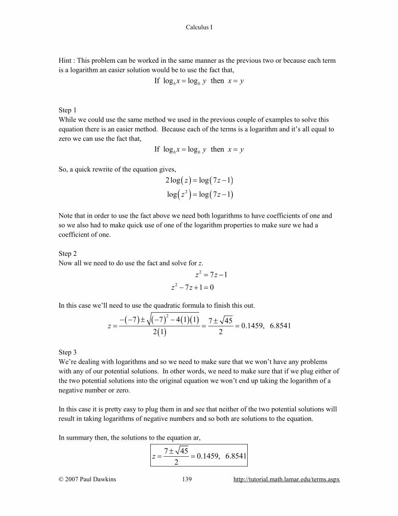
Calculus I
© 2007 Paul Dawkins 139 http://tutorial.math.lamar.edu/terms.aspx
Hint : This problem can be worked in the same manner as the previous two or because each term is a logarithm an easier solution would be to use the fact that, If log log then b bx y x y= = Step 1 While we could use the same method we used in the previous couple of examples to solve this equation there is an easier method. Because each of the terms is a logarithm and it’s all equal to zero we can use the fact that, If log log then b bx y x y= = So, a quick rewrite of the equation gives,
( ) ( )
( ) ( )2
2log log 7 1
log log 7 1
z z
z z
= −
= −
Note that in order to use the fact above we need both logarithms to have coefficients of one and so we also had to make quick use of one of the logarithm properties to make sure we had a coefficient of one. Step 2 Now all we need to do use the fact and solve for z.
2
2
7 17 1 0
z zz z
= −
− + =
In this case we’ll need to use the quadratic formula to finish this out.
( ) ( ) ( )( )
( )
27 7 4 1 1 7 45 0.1459, 6.85412 1 2
z− − ± − − ±
= = =
Step 3 We’re dealing with logarithms and so we need to make sure that we won’t have any problems with any of our potential solutions. In other words, we need to make sure that if we plug either of the two potential solutions into the original equation we won’t end up taking the logarithm of a negative number or zero. In this case it is pretty easy to plug them in and see that neither of the two potential solutions will result in taking logarithms of negative numbers and so both are solutions to the equation. In summary then, the solutions to the equation ar,
7 45 0.1459, 6.85412
z ±= =
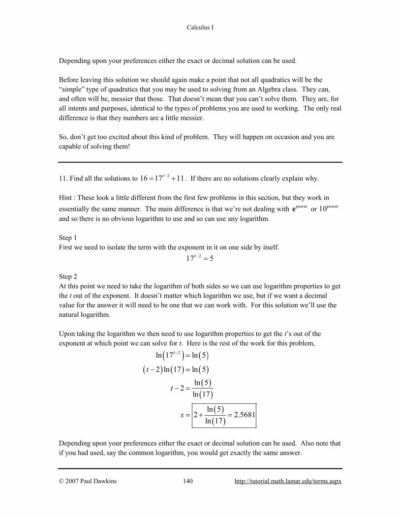
Calculus I
© 2007 Paul Dawkins 140 http://tutorial.math.lamar.edu/terms.aspx
Depending upon your preferences either the exact or decimal solution can be used. Before leaving this solution we should again make a point that not all quadratics will be the “simple” type of quadratics that you may be used to solving from an Algebra class. They can, and often will be, messier that those. That doesn’t mean that you can’t solve them. They are, for all intents and purposes, identical to the types of problems you are used to working. The only real difference is that they numbers are a little messier. So, don’t get too excited about this kind of problem. They will happen on occasion and you are capable of solving them! 11. Find all the solutions to 216 17 11t−= + . If there are no solutions clearly explain why. Hint : These look a little different from the first few problems in this section, but they work in essentially the same manner. The main difference is that we’re not dealing with powere or power10 and so there is no obvious logarithm to use and so can use any logarithm. Step 1 First we need to isolate the term with the exponent in it on one side by itself. 217 5t− = Step 2 At this point we need to take the logarithm of both sides so we can use logarithm properties to get the t out of the exponent. It doesn’t matter which logarithm we use, but if we want a decimal value for the answer it will need to be one that we can work with. For this solution we’ll use the natural logarithm. Upon taking the logarithm we then need to use logarithm properties to get the t’s out of the exponent at which point we can solve for t. Here is the rest of the work for this problem,
( ) ( )( ) ( ) ( )
( )( )
( )( )
2ln 17 ln 5
2 ln 17 ln 5
ln 52
ln 17
ln 52 2.5681
ln 17
t
t
t
x
− =
− =
− =
= + =
Depending upon your preferences either the exact or decimal solution can be used. Also note that if you had used, say the common logarithm, you would get exactly the same answer.

Calculus I
© 2007 Paul Dawkins 141 http://tutorial.math.lamar.edu/terms.aspx
12. Find all the solutions to 3 82 7 11w− − = . If there are no solutions clearly explain why. Hint : These look a little different from the first few problems in this section, but they work in essentially the same manner. The main difference is that we’re not dealing with powere or power10 and so there is no obvious logarithm to use and so can use any logarithm. Step 1 First we need to isolate the term with the exponent in it on one side by itself. 3 82 18w− = Step 2 At this point we need to take the logarithm of both sides so we can use logarithm properties to get the w out of the exponent. It doesn’t matter which logarithm we use, but if we want a decimal value for the answer it will need to be one that we can work with. For this solution we’ll use the natural logarithm. Upon taking the logarithm we then need to use logarithm properties to get the w’s out of the exponent at which point we can solve for w. Here is the rest of the work for this problem,
( ) ( )( ) ( ) ( )
( )( )
( )( )
3 8ln 2 ln 18
3 8 ln 2 ln 18
ln 183 8
ln 2
ln 181 3 0.14628 ln 2
w
w
w
w
− =
− =
− =
= − = −
Depending upon your preferences either the exact or decimal solution can be used. Also note that if you had used, say the common logarithm, you would get exactly the same answer. Compound Interest. If we put P dollars into an account that earns interest at a rate of r (written as a decimal as opposed to the standard percent) for t years then,
a. if interest is compounded m times per year we will have,
1t mrA P
m = +
dollars after t years.
b. if interest is compounded continuously we will have, r tA P= e
dollars after t years.
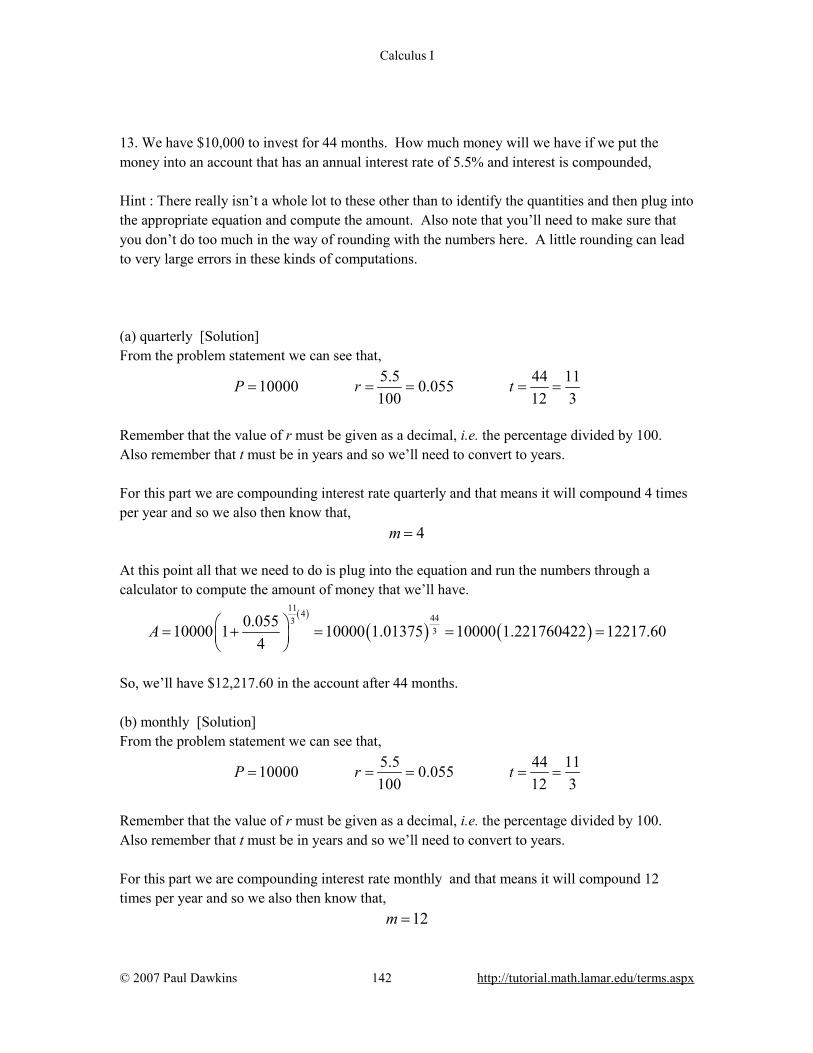
Calculus I
© 2007 Paul Dawkins 142 http://tutorial.math.lamar.edu/terms.aspx
13. We have $10,000 to invest for 44 months. How much money will we have if we put the money into an account that has an annual interest rate of 5.5% and interest is compounded, Hint : There really isn’t a whole lot to these other than to identify the quantities and then plug into the appropriate equation and compute the amount. Also note that you’ll need to make sure that you don’t do too much in the way of rounding with the numbers here. A little rounding can lead to very large errors in these kinds of computations. (a) quarterly [Solution] From the problem statement we can see that,
5.5 44 1110000 0.055100 12 3
P r t= = = = =
Remember that the value of r must be given as a decimal, i.e. the percentage divided by 100. Also remember that t must be in years and so we’ll need to convert to years. For this part we are compounding interest rate quarterly and that means it will compound 4 times per year and so we also then know that, 4m = At this point all that we need to do is plug into the equation and run the numbers through a calculator to compute the amount of money that we’ll have.
( )
( ) ( )11 4 443
30.05510000 1 10000 1.01375 10000 1.221760422 12217.60
4A = + = = =
So, we’ll have $12,217.60 in the account after 44 months. (b) monthly [Solution] From the problem statement we can see that,
5.5 44 1110000 0.055100 12 3
P r t= = = = =
Remember that the value of r must be given as a decimal, i.e. the percentage divided by 100. Also remember that t must be in years and so we’ll need to convert to years. For this part we are compounding interest rate monthly and that means it will compound 12 times per year and so we also then know that, 12m =
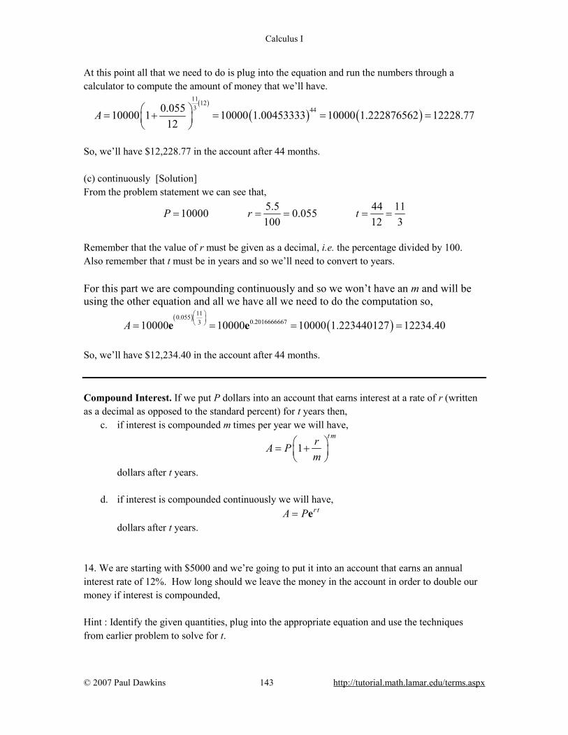
Calculus I
© 2007 Paul Dawkins 143 http://tutorial.math.lamar.edu/terms.aspx
At this point all that we need to do is plug into the equation and run the numbers through a calculator to compute the amount of money that we’ll have.
( )
( ) ( )11 123 440.05510000 1 10000 1.00453333 10000 1.222876562 12228.77
12A = + = = =
So, we’ll have $12,228.77 in the account after 44 months. (c) continuously [Solution] From the problem statement we can see that,
5.5 44 1110000 0.055100 12 3
P r t= = = = =
Remember that the value of r must be given as a decimal, i.e. the percentage divided by 100. Also remember that t must be in years and so we’ll need to convert to years. For this part we are compounding continuously and so we won’t have an m and will be using the other equation and all we have all we need to do the computation so,
( )
( )110.055
0.2016666667310000 10000 10000 1.223440127 12234.40A = = = =e e
So, we’ll have $12,234.40 in the account after 44 months. Compound Interest. If we put P dollars into an account that earns interest at a rate of r (written as a decimal as opposed to the standard percent) for t years then,
c. if interest is compounded m times per year we will have,
1t mrA P
m = +
dollars after t years.
d. if interest is compounded continuously we will have, r tA P= e
dollars after t years. 14. We are starting with $5000 and we’re going to put it into an account that earns an annual interest rate of 12%. How long should we leave the money in the account in order to double our money if interest is compounded, Hint : Identify the given quantities, plug into the appropriate equation and use the techniques from earlier problem to solve for t.
Calculus I
© 2007 Paul Dawkins 144 http://tutorial.math.lamar.edu/terms.aspx
(a) quarterly [Solution] From the problem statement we can see that,
1210000 5000 0.12100
A P r= = = =
Remember that the value of r must be given as a decimal, i.e. the percentage divided by 100. Also, for this part we are compounding interest rate quarterly and that means it will compound 4 times per year and so we also then know that, 4m = Plugging into the equation gives us,
( )4
40.1210000 5000 1 5000 1.034
tt = + =
Using the techniques from this section we can solve for t.
( ) ( )( ) ( )
( )( )
4
4
2 1.03
ln 2 ln 1.03
ln 2 4 ln 1.03
ln 25.8624
4ln 1.03
t
t
t
t
=
=
=
= =
So, we’ll double our money in approximately 5.8624 years. (b) monthly [Solution] From the problem statement we can see that,
1210000 5000 0.12100
A P r= = = =
Remember that the value of r must be given as a decimal, i.e. the percentage divided by 100. Also, for this part we are compounding interest rate monthly and that means it will compound 12 times per year and so we also then know that, 12m = Plugging into the equation gives us,
( )12
120.1210000 5000 1 5000 1.0112
tt = + =
Using the techniques from this section we can solve for t.
Calculus I
© 2007 Paul Dawkins 145 http://tutorial.math.lamar.edu/terms.aspx
( ) ( )( ) ( )
( )( )
12
12
2 1.01
ln 2 ln 1.01
ln 2 12 ln 1.01
ln 25.8051
12ln 1.01
t
t
t
t
=
=
=
= =
So, we’ll double our money in approximately 5.8624 years. (c) continuously [Solution] From the problem statement we can see that,
1210000 5000 0.12100
A P r= = = =
Remember that the value of r must be given as a decimal, i.e. the percentage divided by 100. For this part we are compounding continuously and so we won’t have an m and will be using the other equation. Plugging into the continuously compounding interest equation gives, 0.1210000 5000 t= e Now, solving this gives,
( ) ( )( )
( )
0.12
0.12
2
ln 2 ln
ln 2 0.12
ln 25.7762
0.12
t
t
t
t
=
=
=
= =
e
e
So, we’ll double our money in approximately 5.7762 years. Exponential Growth/Decay. Many quantities in the world can be modeled (at least for a short time) by the exponential growth/decay equation. 0
k tQ Q= e If k is positive then we will get exponential growth and if k is negative we will get exponential decay. 15. A population of bacteria initially has 250 present and in 5 days there will be 1600 bacteria present.
Calculus I
© 2007 Paul Dawkins 146 http://tutorial.math.lamar.edu/terms.aspx
(a) Determine the exponential growth equation for this population. Hint : We have an equation with two unknowns and two values of the population at two times so use these values to find the two unknowns. [Solution] We can start off here by acknowledging that we know, ( ) ( )0 250 and 5 1600Q Q= = If we use the first condition in the equation we get,
( ) ( )00 0 0250 0 250kQ Q Q Q= = = → =e
We now know the first unknown in the equation. Plugging this as well as the second condition into the equation gives us, ( ) 51600 5 250 kQ= = e We can use techniques from earlier problems in this section to determine the value of k.
5
5
1600 250160025032ln 55
1 32ln 0.37125965 5
k
k
k
k
=
=
=
= =
e
e
Depending upon your preferences we can use either the exact value or the decimal value. Note however that because k is in the exponent of an exponential function we’ll need to use quite a few decimal places to avoid potentially large differences in the value that we’d get if we rounded off too much. Putting all of this together the exponential growth equation for this population is,
1 32ln5 5250
tQ
= e
(b) How long will it take for the population to grow from its initial population of 250 to a population of 2000? [Solution] What we’re really being asked to do here is to solve the equation,
( )1 32ln5 52000 250
tQ t
= = e
Calculus I
© 2007 Paul Dawkins 147 http://tutorial.math.lamar.edu/terms.aspx
and we know from earlier problems in this section how to do that. Here is the solution work for this part.
( )
( )( )
1 32ln5 5
325
2000250
1 32ln 8 ln5 5
5ln 85.6010
ln
t
t
t
=
=
= =
e
It will take 5.601 days for the population to reach 2000. Exponential Growth/Decay. Many quantities in the world can be modeled (at least for a short time) by the exponential growth/decay equation. 0
k tQ Q= e If k is positive then we will get exponential growth and if k is negative we will get exponential decay. 16. We initially have 100 grams of a radioactive element and in 1250 years there will be 80 grams left. (a) Determine the exponential decay equation for this element. Hint : We have an equation with two unknowns and two values of the amount of the element left at two times so use these values to find the two unknowns. [Solution] We can start off here by acknowledging that we know, ( ) ( )0 100 and 1250 80Q Q= = If we use the first condition in the equation we get,
( ) ( )00 0 0100 0 100kQ Q Q Q= = = → =e
We now know the first unknown in the equation. Plugging this as well as the second condition into the equation gives us, ( ) 125080 1250 100 kQ= = e We can use techniques from earlier problems in this section to determine the value of k.
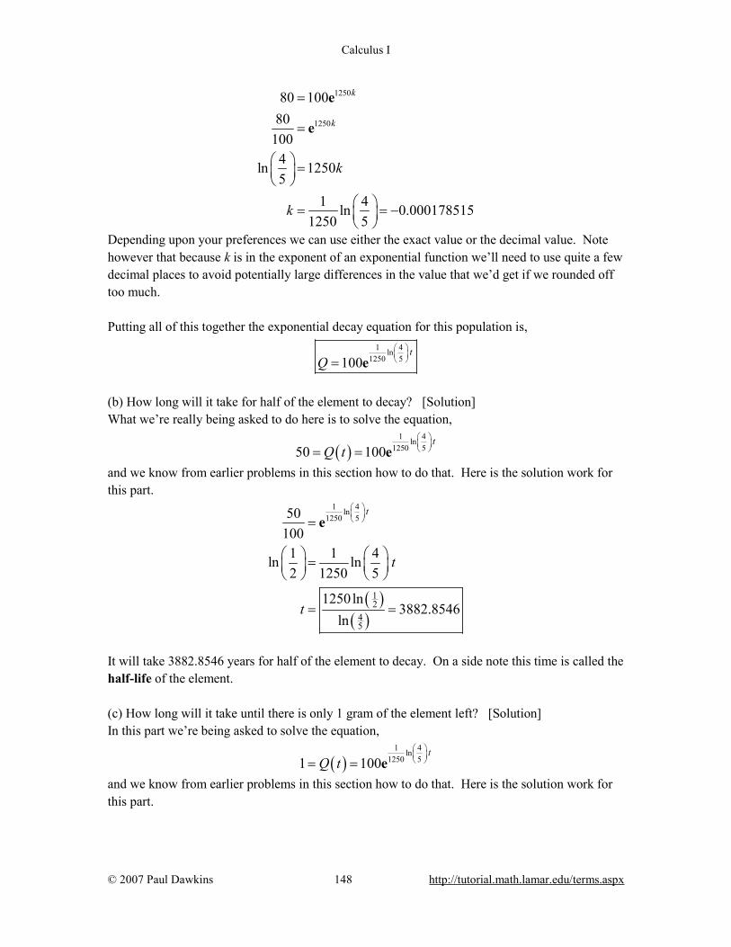
Calculus I
© 2007 Paul Dawkins 148 http://tutorial.math.lamar.edu/terms.aspx
1250
1250
80 10080
1004ln 12505
1 4ln 0.0001785151250 5
k
k
k
k
=
=
=
= = −
e
e
Depending upon your preferences we can use either the exact value or the decimal value. Note however that because k is in the exponent of an exponential function we’ll need to use quite a few decimal places to avoid potentially large differences in the value that we’d get if we rounded off too much. Putting all of this together the exponential decay equation for this population is,
1 4ln
1250 5100t
Q = e
(b) How long will it take for half of the element to decay? [Solution] What we’re really being asked to do here is to solve the equation,
( )1 4ln
1250 550 100t
Q t = = e
and we know from earlier problems in this section how to do that. Here is the solution work for this part.
( )( )
1 4ln1250 5
12
45
501001 1 4ln ln2 1250 5
1250ln3882.8546
ln
t
t
t
=
=
= =
e
It will take 3882.8546 years for half of the element to decay. On a side note this time is called the half-life of the element. (c) How long will it take until there is only 1 gram of the element left? [Solution] In this part we’re being asked to solve the equation,
( )1 4ln
1250 51 100t
Q t = = e
and we know from earlier problems in this section how to do that. Here is the solution work for this part.

Calculus I
© 2007 Paul Dawkins 149 http://tutorial.math.lamar.edu/terms.aspx
( )( )
1 4ln1250 5
1100
45
11001 1 4ln ln
100 1250 5
1250ln25797.1279
ln
t
t
t
=
=
= =
e
There will only be 1 gram of the element left aft 25,797.1279 years.
Review : Common Graphs
1. Without using a graphing calculator sketch the graph of 4 23
y x= − .
Solution
This is just a line with slope 43
and y-intercept ( )0, 2− so here is the graph.
2. Without using a graphing calculator sketch the graph of ( ) 3f x x= − .
Hint : Recall that the graph of ( )g x c+ is simply the graph of ( )g x shifted right by c units if
0c < or shifted left by c units if 0c > .

Calculus I
© 2007 Paul Dawkins 150 http://tutorial.math.lamar.edu/terms.aspx
Solution Recall the basic Algebraic transformations. If we know the graph of ( )g x then the graph of
( )g x c+ is simply the graph of ( )g x shifted right by c units if 0c < or shifted left by c units if
0c > . So, in our case if ( )g x x= we can see that,
( ) ( )3 3f x x g x= − = − and so the graph we’re being asked to sketch is the graph of the absolute value function shifted right by 3 units. Here is the graph of ( ) 3f x x= − and note that to help see the transformation we have also
sketched in the graph of ( )g x x= .
3. Without using a graphing calculator sketch the graph of ( ) ( )sin 6g x x= + .
Hint : Recall that the graph of ( )f x c+ is simply the graph of ( )f x shifted down by c units if
0c < or shifted up by c units if 0c > . Solution Recall the basic Algebraic transformations. If we know the graph of ( )f x then the graph of
( )f x c+ is simply the graph of ( )f x shifted down by c units if 0c < or shifted up by c units
if 0c > .
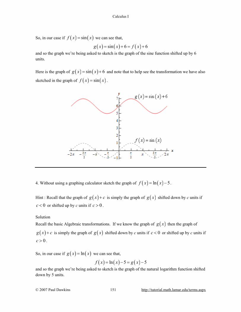
Calculus I
© 2007 Paul Dawkins 151 http://tutorial.math.lamar.edu/terms.aspx
So, in our case if ( ) ( )sinf x x= we can see that,
( ) ( ) ( )sin 6 6g x x f x= + = + and so the graph we’re being asked to sketch is the graph of the sine function shifted up by 6 units. Here is the graph of ( ) ( )sin 6g x x= + and note that to help see the transformation we have also
sketched in the graph of ( ) ( )sinf x x= .
4. Without using a graphing calculator sketch the graph of ( ) ( )ln 5f x x= − .
Hint : Recall that the graph of ( )g x c+ is simply the graph of ( )g x shifted down by c units if
0c < or shifted up by c units if 0c > . Solution Recall the basic Algebraic transformations. If we know the graph of ( )g x then the graph of
( )g x c+ is simply the graph of ( )g x shifted down by c units if 0c < or shifted up by c units if
0c > . So, in our case if ( ) ( )lng x x= we can see that,
( ) ( ) ( )ln 5 5f x x g x= − = − and so the graph we’re being asked to sketch is the graph of the natural logarithm function shifted down by 5 units.
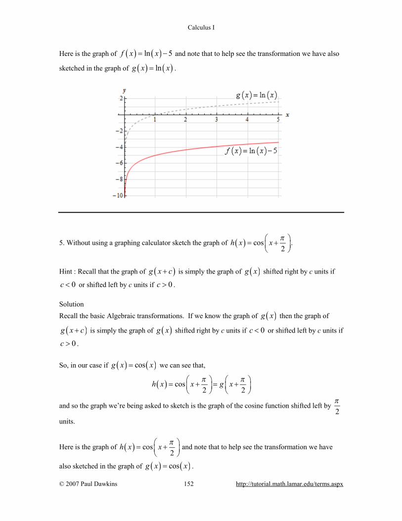
Calculus I
© 2007 Paul Dawkins 152 http://tutorial.math.lamar.edu/terms.aspx
Here is the graph of ( ) ( )ln 5f x x= − and note that to help see the transformation we have also
sketched in the graph of ( ) ( )lng x x= .
5. Without using a graphing calculator sketch the graph of ( ) cos2
h x x π = +
.
Hint : Recall that the graph of ( )g x c+ is simply the graph of ( )g x shifted right by c units if
0c < or shifted left by c units if 0c > . Solution Recall the basic Algebraic transformations. If we know the graph of ( )g x then the graph of
( )g x c+ is simply the graph of ( )g x shifted right by c units if 0c < or shifted left by c units if
0c > . So, in our case if ( ) ( )cosg x x= we can see that,
( ) cos2 2
h x x g xπ π = + = +
and so the graph we’re being asked to sketch is the graph of the cosine function shifted left by 2π
units.
Here is the graph of ( ) cos2
h x x π = +
and note that to help see the transformation we have
also sketched in the graph of ( ) ( )cosg x x= .
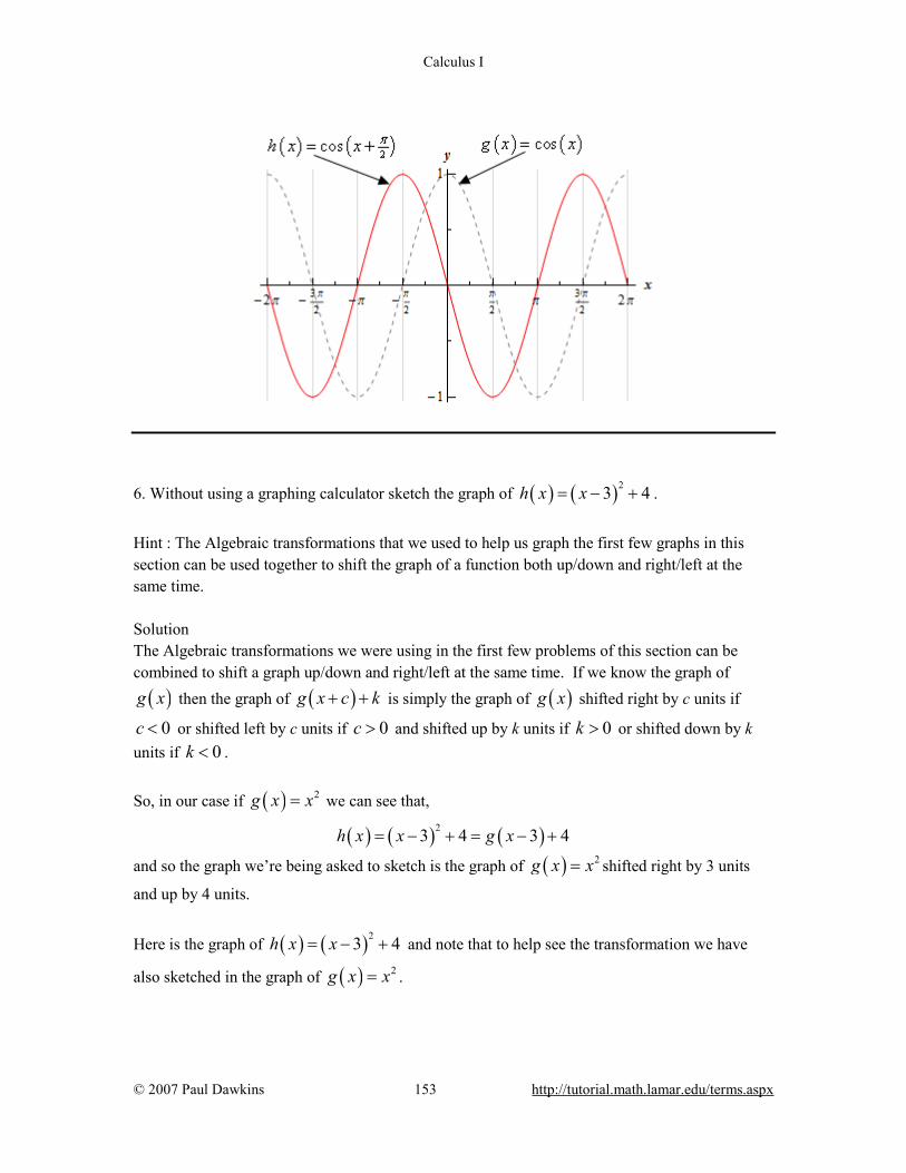
Calculus I
© 2007 Paul Dawkins 153 http://tutorial.math.lamar.edu/terms.aspx
6. Without using a graphing calculator sketch the graph of ( ) ( )23 4h x x= − + .
Hint : The Algebraic transformations that we used to help us graph the first few graphs in this section can be used together to shift the graph of a function both up/down and right/left at the same time. Solution The Algebraic transformations we were using in the first few problems of this section can be combined to shift a graph up/down and right/left at the same time. If we know the graph of
( )g x then the graph of ( )g x c k+ + is simply the graph of ( )g x shifted right by c units if
0c < or shifted left by c units if 0c > and shifted up by k units if 0k > or shifted down by k units if 0k < . So, in our case if ( ) 2g x x= we can see that,
( ) ( ) ( )23 4 3 4h x x g x= − + = − +
and so the graph we’re being asked to sketch is the graph of ( ) 2g x x= shifted right by 3 units
and up by 4 units.
Here is the graph of ( ) ( )23 4h x x= − + and note that to help see the transformation we have
also sketched in the graph of ( ) 2g x x= .
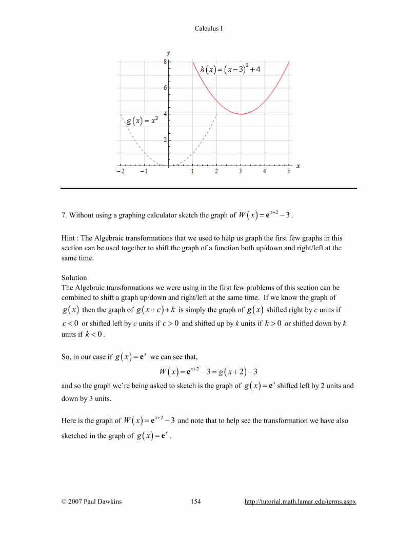
Calculus I
© 2007 Paul Dawkins 154 http://tutorial.math.lamar.edu/terms.aspx
7. Without using a graphing calculator sketch the graph of ( ) 2 3xW x += −e .
Hint : The Algebraic transformations that we used to help us graph the first few graphs in this section can be used together to shift the graph of a function both up/down and right/left at the same time. Solution The Algebraic transformations we were using in the first few problems of this section can be combined to shift a graph up/down and right/left at the same time. If we know the graph of
( )g x then the graph of ( )g x c k+ + is simply the graph of ( )g x shifted right by c units if
0c < or shifted left by c units if 0c > and shifted up by k units if 0k > or shifted down by k units if 0k < . So, in our case if ( ) xg x = e we can see that,
( ) ( )2 3 2 3xW x g x+= − = + −e
and so the graph we’re being asked to sketch is the graph of ( ) xg x = e shifted left by 2 units and
down by 3 units. Here is the graph of ( ) 2 3xW x += −e and note that to help see the transformation we have also
sketched in the graph of ( ) xg x = e .
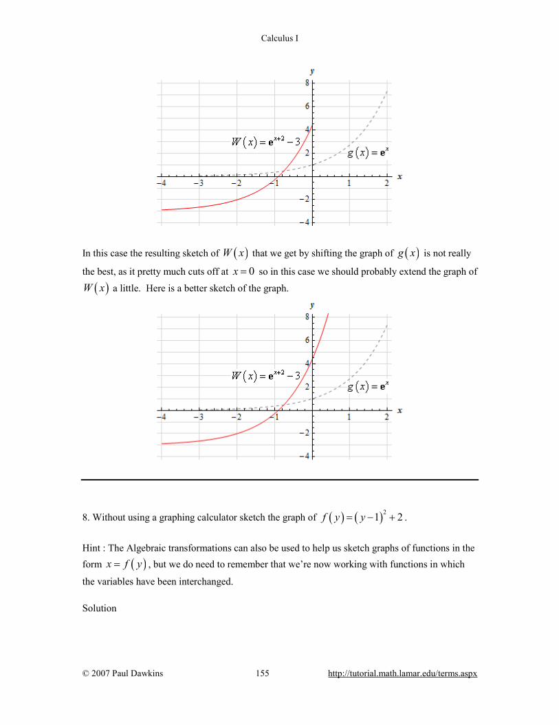
Calculus I
© 2007 Paul Dawkins 155 http://tutorial.math.lamar.edu/terms.aspx
In this case the resulting sketch of ( )W x that we get by shifting the graph of ( )g x is not really
the best, as it pretty much cuts off at 0x = so in this case we should probably extend the graph of
( )W x a little. Here is a better sketch of the graph.
8. Without using a graphing calculator sketch the graph of ( ) ( )21 2f y y= − + .
Hint : The Algebraic transformations can also be used to help us sketch graphs of functions in the form ( )x f y= , but we do need to remember that we’re now working with functions in which
the variables have been interchanged. Solution
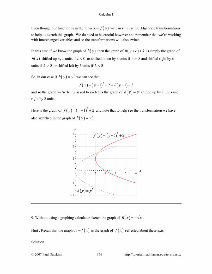
Calculus I
© 2007 Paul Dawkins 156 http://tutorial.math.lamar.edu/terms.aspx
Even though our function is in the form ( )x f y= we can still use the Algebraic transformations
to help us sketch this graph. We do need to be careful however and remember that we’re working with interchanged variables and so the transformations will also switch. In this case if we know the graph of ( )h y then the graph of ( )h y c k+ + is simply the graph of
( )h x shifted up by c units if 0c < or shifted down by c units if 0c > and shifted right by k
units if 0k > or shifted left by k units if 0k < . So, in our case if ( ) 2h y y= we can see that,
( ) ( ) ( )21 2 1 2f y y h y= − + = − +
and so the graph we’re being asked to sketch is the graph of ( ) 2h y y= shifted up by 1 units and
right by 2 units.
Here is the graph of ( ) ( )21 2f y y= − + and note that to help see the transformation we have
also sketched in the graph of ( ) 2h y y= .
9. Without using a graphing calculator sketch the graph of ( )R x x= − .
Hint : Recall that the graph of ( )f x− is the graph of ( )f x reflected about the x-axis.
Solution
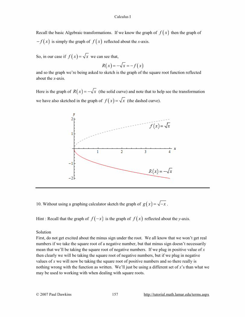
Calculus I
© 2007 Paul Dawkins 157 http://tutorial.math.lamar.edu/terms.aspx
Recall the basic Algebraic transformations. If we know the graph of ( )f x then the graph of
( )f x− is simply the graph of ( )f x reflected about the x-axis.
So, in our case if ( )f x x= we can see that,
( ) ( )R x x f x= − = − and so the graph we’re being asked to sketch is the graph of the square root function reflected about the x-axis.
Here is the graph of ( )R x x= − (the solid curve) and note that to help see the transformation
we have also sketched in the graph of ( )f x x= (the dashed curve).
10. Without using a graphing calculator sketch the graph of ( )g x x= − .
Hint : Recall that the graph of ( )f x− is the graph of ( )f x reflected about the y-axis.
Solution First, do not get excited about the minus sign under the root. We all know that we won’t get real numbers if we take the square root of a negative number, but that minus sign doesn’t necessarily mean that we’ll be taking the square root of negative numbers. If we plug in positive value of x then clearly we will be taking the square root of negative numbers, but if we plug in negative values of x we will now be taking the square root of positive numbers and so there really is nothing wrong with the function as written. We’ll just be using a different set of x’s than what we may be used to working with when dealing with square roots.

Calculus I
© 2007 Paul Dawkins 158 http://tutorial.math.lamar.edu/terms.aspx
Now, recall the basic Algebraic transformations. If we know the graph of ( )f x then the graph
of ( )f x− is simply the graph of ( )f x reflected about the y-axis.
So, in our case if ( )f x x= we can see that,
( ) ( )g x x f x= − = − and so the graph we’re being asked to sketch is the graph of the square root function reflected about the y-axis.
Here is the graph of ( )g x x= − and note that to help see the transformation we have also
sketched in the graph of ( )f x x= .
11. Without using a graphing calculator sketch the graph of ( ) 22 3 4h x x x= − + .
Hint : Recall that the graph of ( ) 2f x ax bx c= + + is the graph of a parabola with vertex
,2 2b bfa a
− − that opens upwards if 0a > and downwards if 0a < and y-intercept at
( )0,c .
Solution We know that the graph of ( ) 2f x ax bx c= + + will be a parabola that opens upwards if 0a >
and opens downwards if 0a < . We also know that its vertex is at,
,2 2b bfa a
− −
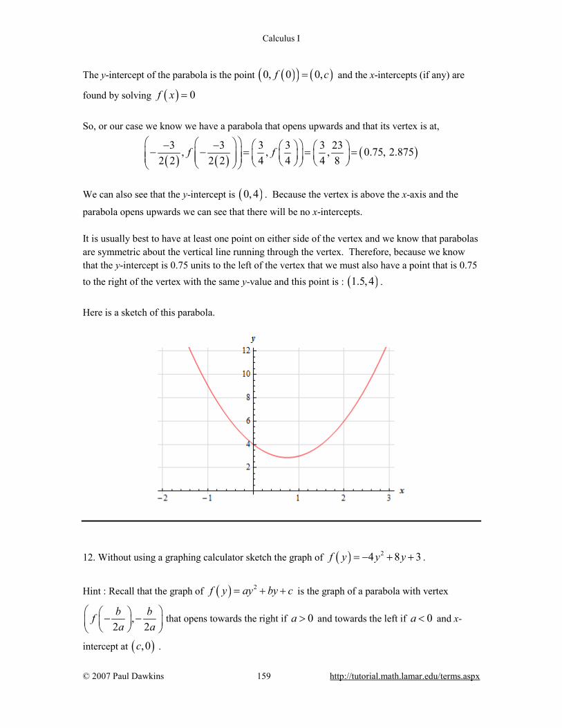
Calculus I
© 2007 Paul Dawkins 159 http://tutorial.math.lamar.edu/terms.aspx
The y-intercept of the parabola is the point ( )( ) ( )0, 0 0,f c= and the x-intercepts (if any) are
found by solving ( ) 0f x =
So, or our case we know we have a parabola that opens upwards and that its vertex is at,
( ) ( ) ( )3 3 3 3 3 23, , , 0.75, 2.875
2 2 2 2 4 4 4 8f f
− − − − = = =
We can also see that the y-intercept is ( )0, 4 . Because the vertex is above the x-axis and the
parabola opens upwards we can see that there will be no x-intercepts. It is usually best to have at least one point on either side of the vertex and we know that parabolas are symmetric about the vertical line running through the vertex. Therefore, because we know that the y-intercept is 0.75 units to the left of the vertex that we must also have a point that is 0.75 to the right of the vertex with the same y-value and this point is : ( )1.5,4 .
Here is a sketch of this parabola.
12. Without using a graphing calculator sketch the graph of ( ) 24 8 3f y y y= − + + .
Hint : Recall that the graph of ( ) 2f y ay by c= + + is the graph of a parabola with vertex
,2 2b bfa a
− − that opens towards the right if 0a > and towards the left if 0a < and x-
intercept at ( ),0c .
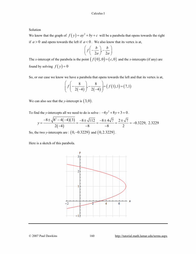
Calculus I
© 2007 Paul Dawkins 160 http://tutorial.math.lamar.edu/terms.aspx
Solution We know that the graph of ( ) 2f y ay by c= + + will be a parabola that opens towards the right
if 0a > and opens towards the left if 0a < . We also know that its vertex is at,
,2 2b bfa a
− −
The x-intercept of the parabola is the point ( )( ) ( )0 ,0 ,0f c= and the x-intercepts (if any) are
found by solving ( ) 0f y =
So, or our case we know we have a parabola that opens towards the left and that its vertex is at,
( ) ( ) ( )( ) ( )8 8, 1 ,1 7,1
2 4 2 4f f
− − = = − −
We can also see that the y-intercept is ( )3,0 .
To find the y-intercepts all we need to do is solve : 24 8 3 0y y− + + = .
( )( )
( )
28 8 4 4 3 8 112 8 4 7 2 7 0.3229, 2.32292 4 8 8 2
y− ± − − − ± − ± ±
= = = = = −− − −
So, the two y-intercepts are : ( )0, 0.3229− and ( )0,2.3229 .
Here is a sketch of this parabola.
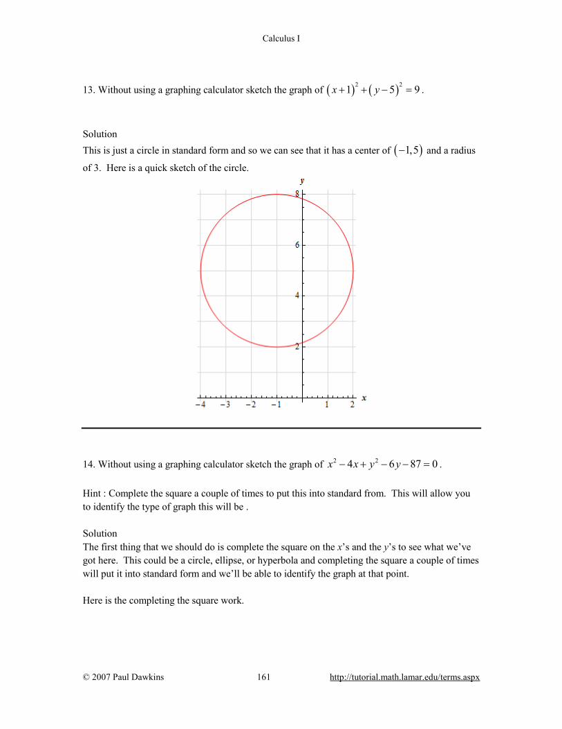
Calculus I
© 2007 Paul Dawkins 161 http://tutorial.math.lamar.edu/terms.aspx
13. Without using a graphing calculator sketch the graph of ( ) ( )2 21 5 9x y+ + − = .
Solution This is just a circle in standard form and so we can see that it has a center of ( )1,5− and a radius
of 3. Here is a quick sketch of the circle.
14. Without using a graphing calculator sketch the graph of 2 24 6 87 0x x y y− + − − = . Hint : Complete the square a couple of times to put this into standard from. This will allow you to identify the type of graph this will be . Solution The first thing that we should do is complete the square on the x’s and the y’s to see what we’ve got here. This could be a circle, ellipse, or hyperbola and completing the square a couple of times will put it into standard form and we’ll be able to identify the graph at that point. Here is the completing the square work.

Calculus I
© 2007 Paul Dawkins 162 http://tutorial.math.lamar.edu/terms.aspx
( ) ( )( ) ( )
( ) ( )
2 2
2 2
2 2
4 4 4 6 9 9 87 0
2 3 100 0
2 3 100
x x y y
x y
x y
− + − + − + − − =
− + − − =
− + − =
So, we’ve got a circle with center ( )2,3 and radius 10. Here is a sketch of the circle.
15. Without using a graphing calculator sketch the graph of ( )2
225 2 116yx + + = .
Solution This is just an ellipse that is almost in standard form. With a little rewrite we can put it into standard form as follows,
( )2 2211 425
x y++ =
We can now see that the ellipse has a center of ( )2,0− while the left/right most points will be
1 0.25
= units away from the center and the top/bottom most points will be 2 units away from the
center. Here is a quick sketch of the ellipse.

Calculus I
© 2007 Paul Dawkins 163 http://tutorial.math.lamar.edu/terms.aspx
16. Without using a graphing calculator sketch the graph of ( )2
2 61
9y
x−
+ = .
Solution
This is just an ellipse that is in standard form (if it helps rewrite the first term as 2
1x
) and so we
can see that it has a center of ( )0,6 while the left/right most points will be 1 unit away from the
center and the top/bottom most points will be 3 units away from the center. Here is a quick sketch of the ellipse.

Calculus I
© 2007 Paul Dawkins 164 http://tutorial.math.lamar.edu/terms.aspx
17. Without using a graphing calculator sketch the graph of 2 2
136 49x y
− = .
Solution This is a hyperbola in standard form with the minus sign in front of the y term and so will open right and left. The center of the hyperbola is at ( )0,0 , the two vertices are at ( )6,0− and ( )6,0
, and the slope of the two asymptotes are 76
± .
Here is a quick sketch of the hyperbola.

Calculus I
© 2007 Paul Dawkins 165 http://tutorial.math.lamar.edu/terms.aspx
18. Without using a graphing calculator sketch the graph of ( ) ( )22 4
2 116
xy
++ − = .
Solution This is a hyperbola in standard form with the minus sign in front of the x term and so will open up and down. The center of the hyperbola is at ( )4, 2− − , the two vertices are at ( )1, 1− − and
( )1, 3− − , and the slope of the two asymptotes are 14
± .
Here is a quick sketch of the hyperbola.
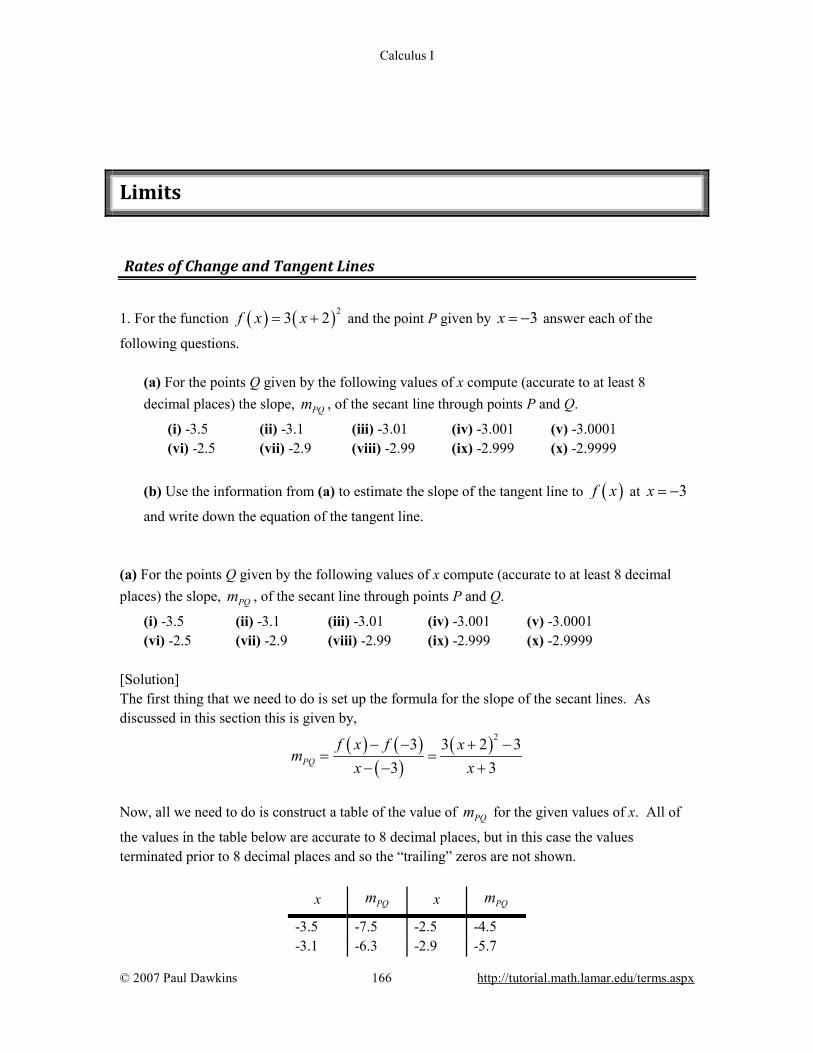
Calculus I
© 2007 Paul Dawkins 166 http://tutorial.math.lamar.edu/terms.aspx
Limits
Rates of Change and Tangent Lines
1. For the function ( ) ( )23 2f x x= + and the point P given by 3x = − answer each of the
following questions.
(a) For the points Q given by the following values of x compute (accurate to at least 8 decimal places) the slope, PQm , of the secant line through points P and Q.
(i) -3.5 (ii) -3.1 (iii) -3.01 (iv) -3.001 (v) -3.0001 (vi) -2.5 (vii) -2.9 (viii) -2.99 (ix) -2.999 (x) -2.9999
(b) Use the information from (a) to estimate the slope of the tangent line to ( )f x at 3x = −
and write down the equation of the tangent line. (a) For the points Q given by the following values of x compute (accurate to at least 8 decimal places) the slope, PQm , of the secant line through points P and Q.
(i) -3.5 (ii) -3.1 (iii) -3.01 (iv) -3.001 (v) -3.0001 (vi) -2.5 (vii) -2.9 (viii) -2.99 (ix) -2.999 (x) -2.9999
[Solution] The first thing that we need to do is set up the formula for the slope of the secant lines. As discussed in this section this is given by,
( ) ( )( )
( )23 3 2 33 3PQ
f x f xm
x x− − + −
= =− − +
Now, all we need to do is construct a table of the value of PQm for the given values of x. All of
the values in the table below are accurate to 8 decimal places, but in this case the values terminated prior to 8 decimal places and so the “trailing” zeros are not shown.
x PQm x PQm
-3.5 -7.5 -2.5 -4.5 -3.1 -6.3 -2.9 -5.7
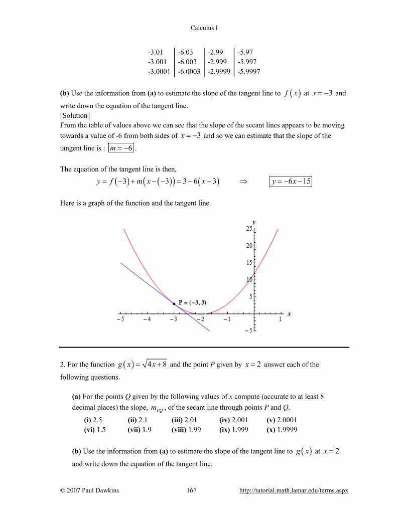
Calculus I
© 2007 Paul Dawkins 167 http://tutorial.math.lamar.edu/terms.aspx
-3.01 -6.03 -2.99 -5.97 -3.001 -6.003 -2.999 -5.997 -3.0001 -6.0003 -2.9999 -5.9997
(b) Use the information from (a) to estimate the slope of the tangent line to ( )f x at 3x = − and
write down the equation of the tangent line. [Solution] From the table of values above we can see that the slope of the secant lines appears to be moving towards a value of -6 from both sides of 3x = − and so we can estimate that the slope of the
tangent line is : 6m = − . The equation of the tangent line is then,
( ) ( )( ) ( )3 3 3 6 3 6 15y f m x x y x= − + − − = − + ⇒ = − − Here is a graph of the function and the tangent line.
2. For the function ( ) 4 8g x x= + and the point P given by 2x = answer each of the
following questions.
(a) For the points Q given by the following values of x compute (accurate to at least 8 decimal places) the slope, PQm , of the secant line through points P and Q.
(i) 2.5 (ii) 2.1 (iii) 2.01 (iv) 2.001 (v) 2.0001 (vi) 1.5 (vii) 1.9 (viii) 1.99 (ix) 1.999 (x) 1.9999
(b) Use the information from (a) to estimate the slope of the tangent line to ( )g x at 2x =
and write down the equation of the tangent line.
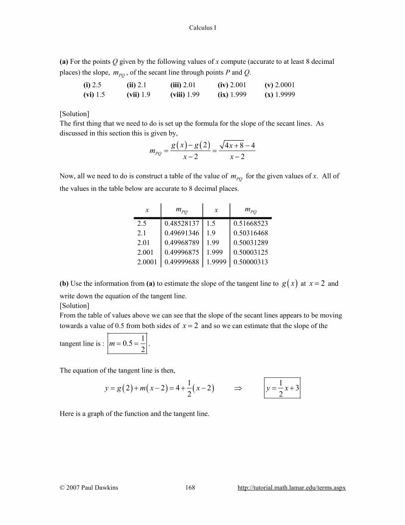
Calculus I
© 2007 Paul Dawkins 168 http://tutorial.math.lamar.edu/terms.aspx
(a) For the points Q given by the following values of x compute (accurate to at least 8 decimal places) the slope, PQm , of the secant line through points P and Q.
(i) 2.5 (ii) 2.1 (iii) 2.01 (iv) 2.001 (v) 2.0001 (vi) 1.5 (vii) 1.9 (viii) 1.99 (ix) 1.999 (x) 1.9999
[Solution] The first thing that we need to do is set up the formula for the slope of the secant lines. As discussed in this section this is given by,
( ) ( )2 4 8 42 2PQ
g x g xmx x
− + −= =
− −
Now, all we need to do is construct a table of the value of PQm for the given values of x. All of
the values in the table below are accurate to 8 decimal places.
x PQm x PQm
2.5 0.48528137 1.5 0.51668523 2.1 0.49691346 1.9 0.50316468 2.01 0.49968789 1.99 0.50031289 2.001 0.49996875 1.999 0.50003125 2.0001 0.49999688 1.9999 0.50000313
(b) Use the information from (a) to estimate the slope of the tangent line to ( )g x at 2x = and
write down the equation of the tangent line. [Solution] From the table of values above we can see that the slope of the secant lines appears to be moving towards a value of 0.5 from both sides of 2x = and so we can estimate that the slope of the
tangent line is : 10.52
m = = .
The equation of the tangent line is then,
( ) ( ) ( )1 12 2 4 2 32 2
y g m x x y x= + − = + − ⇒ = +
Here is a graph of the function and the tangent line.
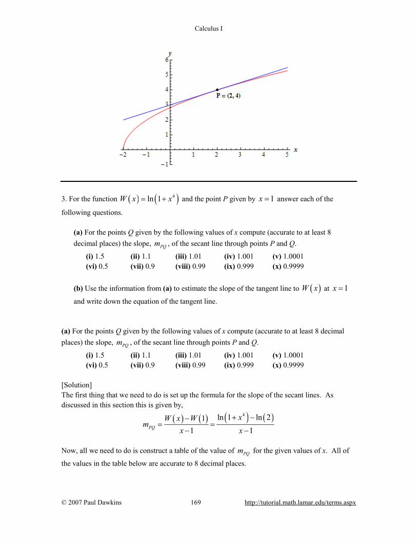
Calculus I
© 2007 Paul Dawkins 169 http://tutorial.math.lamar.edu/terms.aspx
3. For the function ( ) ( )4ln 1W x x= + and the point P given by 1x = answer each of the
following questions.
(a) For the points Q given by the following values of x compute (accurate to at least 8 decimal places) the slope, PQm , of the secant line through points P and Q.
(i) 1.5 (ii) 1.1 (iii) 1.01 (iv) 1.001 (v) 1.0001 (vi) 0.5 (vii) 0.9 (viii) 0.99 (ix) 0.999 (x) 0.9999
(b) Use the information from (a) to estimate the slope of the tangent line to ( )W x at 1x =
and write down the equation of the tangent line. (a) For the points Q given by the following values of x compute (accurate to at least 8 decimal places) the slope, PQm , of the secant line through points P and Q.
(i) 1.5 (ii) 1.1 (iii) 1.01 (iv) 1.001 (v) 1.0001 (vi) 0.5 (vii) 0.9 (viii) 0.99 (ix) 0.999 (x) 0.9999
[Solution] The first thing that we need to do is set up the formula for the slope of the secant lines. As discussed in this section this is given by,
( ) ( ) ( ) ( )4ln 1 ln 211 1PQ
xW x Wm
x x+ −−
= =− −
Now, all we need to do is construct a table of the value of PQm for the given values of x. All of
the values in the table below are accurate to 8 decimal places.

Calculus I
© 2007 Paul Dawkins 170 http://tutorial.math.lamar.edu/terms.aspx
x PQm x PQm
1.5 2.21795015 0.5 1.26504512 1.1 2.08679449 0.9 1.88681740 1.01 2.00986668 0.99 1.98986668 1.001 2.00099867 0.999 1.99899867 1.0001 2.00009999 0.9999 1.99989999
(b) Use the information from (a) to estimate the slope of the tangent line to ( )W x at 1x = and
write down the equation of the tangent line. [Solution] From the table of values above we can see that the slope of the secant lines appears to be moving towards a value of 2 from both sides of 1x = and so we can estimate that the slope of the tangent
line is : 2m = . The equation of the tangent line is then,
( ) ( ) ( ) ( )1 1 ln 2 2 1y W m x x= + − = + − Here is a graph of the function and the tangent line.
4. The volume of air in a balloon is given by ( ) 64 1
V tt
=+
answer each of the following
questions.
(a) Compute (accurate to at least 8 decimal places) the average rate of change of the volume of air in the balloon between 0.25t = and the following values of t.
(i) 1 (ii) 0.5 (iii) 0.251 (iv) 0.2501 (v) 0.25001

Calculus I
© 2007 Paul Dawkins 171 http://tutorial.math.lamar.edu/terms.aspx
(vi) 0 (vii) 0.1 (viii) 0.249 (ix) 0.2499 (x) 0.24999
(b) Use the information from (a) to estimate the instantaneous rate of change of the volume of air in the balloon at 0.25t = .
(a) Compute (accurate to at least 8 decimal places) the average rate of change of the volume of air in the balloon between 0.25t = and the following values of t.
(i) 1 (ii) 0.5 (iii) 0.251 (iv) 0.2501 (v) 0.25001 (vi) 0 (vii) 0.1 (viii) 0.249 (ix) 0.2499 (x) 0.24999
[Solution] The first thing that we need to do is set up the formula for the slope of the secant lines. As discussed in this section this is given by,
( ) ( )6 30.25 4 1
0.25 0.25V t V tARC
t t
−− += =− −
Now, all we need to do is construct a table of the value of PQm for the given values of x. All of
the values in the table below are accurate to 8 decimal places. In several of the initial values in the table the values terminated and so the “trailing” zeroes were not shown.
x ARC x ARC 1 -2.4 0 -12 0.5 -4 0.1 -8.57142857 0.251 -5.98802395 0.249 -6.01202405 0.2501 -5.99880024 0.2499 -6.00120024 0.25001 -5.99988000 0.24999 -6.00012000
(b) Use the information from (a) to estimate the instantaneous rate of change of the volume of air in the balloon at 0.25t = . [Solution] From the table of values above we can see that the average rate of change of the volume of air is moving towards a value of -6 from both sides of 0.25t = and so we can estimate that the instantaneous rate of change of the volume of air in the balloon is 6− . 5. The population (in hundreds) of fish in a pond is given by ( ) ( )2 sin 2 10P t t t= + − answer
each of the following questions.

Calculus I
© 2007 Paul Dawkins 172 http://tutorial.math.lamar.edu/terms.aspx
(a) Compute (accurate to at least 8 decimal places) the average rate of change of the population of fish between 5t = and the following values of t. Make sure your calculator is set to radians for the computations.
(i) 5.5 (ii) 5.1 (iii) 5.01 (iv) 5.001 (v) 5.0001 (vi) 4.5 (vii) 4.9 (viii) 4.99 (ix) 4.999 (x) 4.9999
(b) Use the information from (a) to estimate the instantaneous rate of change of the population of the fish at 5t = .
(a) Compute (accurate to at least 8 decimal places) the average rate of change of the population of fish between 5t = and the following values of t. Make sure your calculator is set to radians for the computations.
(i) 5.5 (ii) 5.1 (iii) 5.01 (iv) 5.001 (v) 5.0001 (vi) 4.5 (vii) 4.9 (viii) 4.99 (ix) 4.999 (x) 4.9999
[Solution] The first thing that we need to do is set up the formula for the slope of the secant lines. As discussed in this section this is given by,
( ) ( ) ( )5 2 sin 2 10 105 5
P t P t tARC
t t− + − −
= =− −
Now, all we need to do is construct a table of the value of PQm for the given values of x. All of
the values in the table below are accurate to 8 decimal places.
x ARC x ARC 5.5 3.68294197 4.5 3.68294197 5.1 3.98669331 4.9 3.98669331 5.01 3.99986667 4.99 3.99986667 5.001 3.99999867 4.999 3.99999867 5.0001 3.99999999 4.9999 3.99999999
(b) Use the information from (a) to estimate the instantaneous rate of change of the population of the fish at 5t = . [Solution] From the table of values above we can see that the average rate of change of the population of fish is moving towards a value of 4 from both sides of 5t = and so we can estimate that the instantaneous rate of change of the volume of air in the balloon is 4.

Calculus I
© 2007 Paul Dawkins 173 http://tutorial.math.lamar.edu/terms.aspx
6. The position of an object is given by ( ) 2 3 6cos2
xs t − =
answer each of the following
questions.
(a) Compute (accurate to at least 8 decimal places) the average velocity of the object between 2t = and the following values of t. Make sure your calculator is set to radians for the
computations. (i) 2.5 (ii) 2.1 (iii) 2.01 (iv) 2.001 (v) 2.0001 (vi) 1.5 (vii) 1.9 (viii) 1.99 (ix) 1.999 (x) 1.9999
(b) Use the information from (a) to estimate the instantaneous velocity of the object at 2t = and determine if the object is moving to the right (i.e. the instantaneous velocity is positive), moving to the left (i.e. the instantaneous velocity is negative), or not moving (i.e. the instantaneous velocity is zero).
(a) Compute (accurate to at least 8 decimal places) the average velocity of the object between
2t = and the following values of t. Make sure your calculator is set to radians for the computations.
(i) 2.5 (ii) 2.1 (iii) 2.01 (iv) 2.001 (v) 2.0001 (vi) 1.5 (vii) 1.9 (viii) 1.99 (ix) 1.999 (x) 1.9999
[Solution] The first thing that we need to do is set up the formula for the slope of the secant lines. As discussed in this section this is given by,
( ) ( )2 3 6cos 12 2
2 2
xs t s
AVt t
− − − = =− −
Now, all we need to do is construct a table of the value of PQm for the given values of x. All of
the values in the table below are accurate to 8 decimal places.
t AV t AV 2.5 -0.92926280 1.5 0.92926280 2.1 -0.22331755 1.9 0.22331755 2.01 -0.02249831 1.99 0.02249831 2.001 -0.00225000 1.999 0.00225000 2.0001 -0.00022500 1.9999 0.00022500
(b) Use the information from (a) to estimate the instantaneous velocity of the object at 2t = and determine if the object is moving to the right (i.e. the instantaneous velocity is positive), moving

Calculus I
© 2007 Paul Dawkins 174 http://tutorial.math.lamar.edu/terms.aspx
to the left (i.e. the instantaneous velocity is negative), or not moving (i.e. the instantaneous velocity is zero). [Solution] From the table of values above we can see that the average velocity of the object is moving towards a value of 0 from both sides of 2t = and so we can estimate that the instantaneous velocity is 0 and so the object will not be moving at 2t = .
7. The position of an object is given by ( ) ( )( )328 6s t x x= − + . Note that a negative position
here simply means that the position is to the left of the “zero position” and is perfectly acceptable. Answer each of the following questions.
(a) Compute (accurate to at least 8 decimal places) the average velocity of the object between 10t = and the following values of t. (i) 10.5 (ii) 10.1 (iii) 10.01 (iv) 10.001 (v) 10.0001 (vi) 9.5 (vii) 9.9 (viii) 9.99 (ix) 9.999 (x) 9.9999
(b) Use the information from (a) to estimate the instantaneous velocity of the object at 10t = and determine if the object is moving to the right (i.e. the instantaneous velocity is positive), moving to the left (i.e. the instantaneous velocity is negative), or not moving (i.e. the instantaneous velocity is zero).
(a) Compute (accurate to at least 8 decimal places) the average velocity of the object between
10t = and the following values of t. (i) 10.5 (ii) 10.1 (iii) 10.01 (iv) 10.001 (v) 10.0001 (vi) 9.5 (vii) 9.9 (viii) 9.99 (ix) 9.999 (x) 9.9999
[Solution] The first thing that we need to do is set up the formula for the slope of the secant lines. As discussed in this section this is given by,
( ) ( ) ( )( )3210 8 6 128
10 10s t s x x
AVt t
− − + += =
− −
Now, all we need to do is construct a table of the value of PQm for the given values of x. All of
the values in the table below are accurate to 8 decimal places.
t AV t AV 10.5 -79.11658419 9.5 -72.92931693 10.1 -76.61966704 9.9 -75.38216890
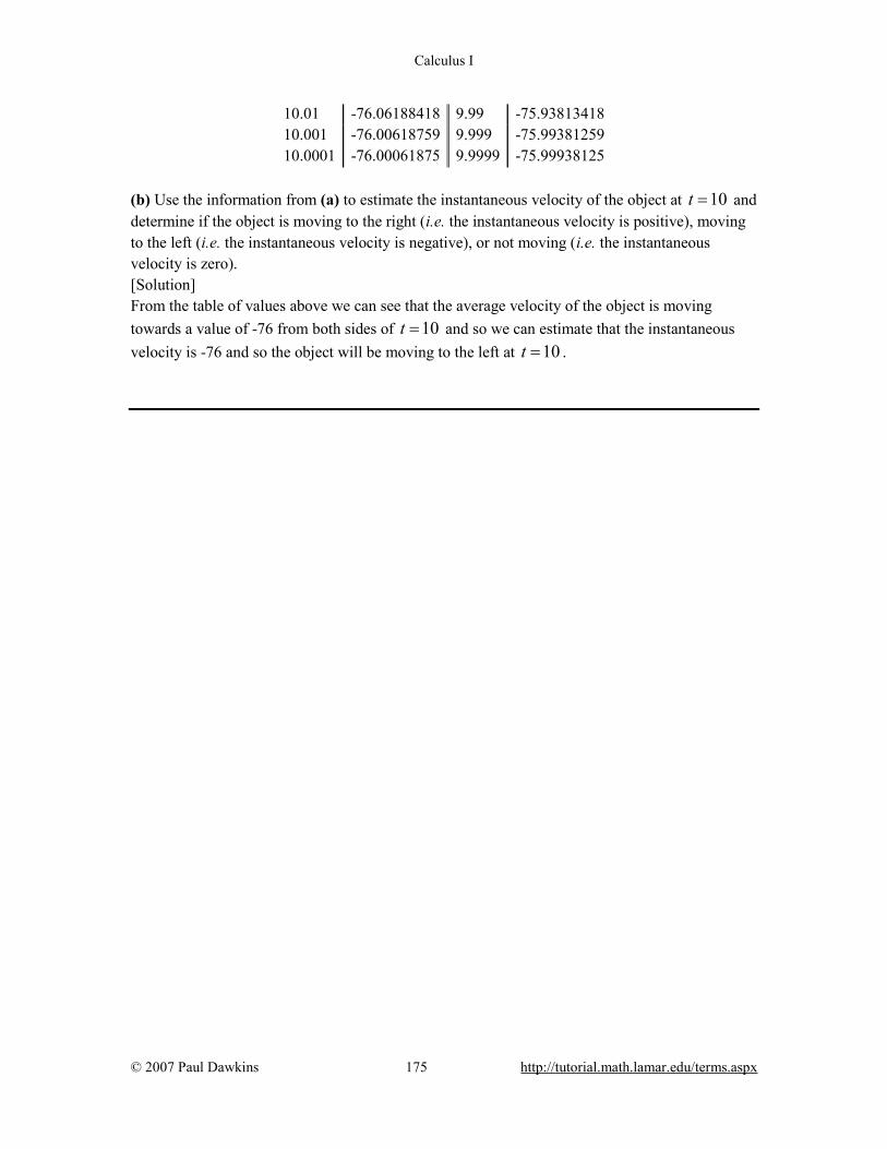
Calculus I
© 2007 Paul Dawkins 175 http://tutorial.math.lamar.edu/terms.aspx
10.01 -76.06188418 9.99 -75.93813418 10.001 -76.00618759 9.999 -75.99381259 10.0001 -76.00061875 9.9999 -75.99938125
(b) Use the information from (a) to estimate the instantaneous velocity of the object at 10t = and determine if the object is moving to the right (i.e. the instantaneous velocity is positive), moving to the left (i.e. the instantaneous velocity is negative), or not moving (i.e. the instantaneous velocity is zero). [Solution] From the table of values above we can see that the average velocity of the object is moving towards a value of -76 from both sides of 10t = and so we can estimate that the instantaneous velocity is -76 and so the object will be moving to the left at 10t = .
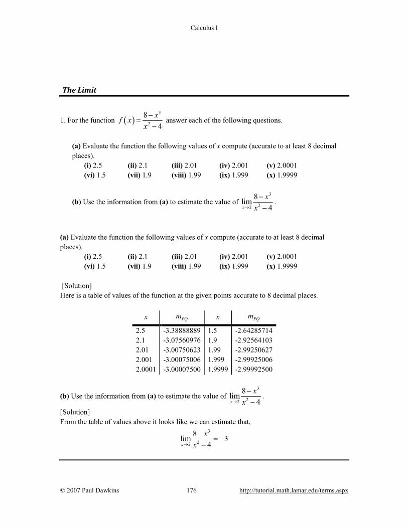
Calculus I
© 2007 Paul Dawkins 176 http://tutorial.math.lamar.edu/terms.aspx
The Limit
1. For the function ( )3
2
84
xf xx
−=
− answer each of the following questions.
(a) Evaluate the function the following values of x compute (accurate to at least 8 decimal places).
(i) 2.5 (ii) 2.1 (iii) 2.01 (iv) 2.001 (v) 2.0001 (vi) 1.5 (vii) 1.9 (viii) 1.99 (ix) 1.999 (x) 1.9999
(b) Use the information from (a) to estimate the value of 3
22
8lim4x
xx→
−−
.
(a) Evaluate the function the following values of x compute (accurate to at least 8 decimal places).
(i) 2.5 (ii) 2.1 (iii) 2.01 (iv) 2.001 (v) 2.0001 (vi) 1.5 (vii) 1.9 (viii) 1.99 (ix) 1.999 (x) 1.9999
[Solution] Here is a table of values of the function at the given points accurate to 8 decimal places.
x PQm x PQm
2.5 -3.38888889 1.5 -2.64285714 2.1 -3.07560976 1.9 -2.92564103 2.01 -3.00750623 1.99 -2.99250627 2.001 -3.00075006 1.999 -2.99925006 2.0001 -3.00007500 1.9999 -2.99992500
(b) Use the information from (a) to estimate the value of 3
22
8lim4x
xx→
−−
.
[Solution] From the table of values above it looks like we can estimate that,
3
22
8lim 34x
xx→
−= −
−

Calculus I
© 2007 Paul Dawkins 177 http://tutorial.math.lamar.edu/terms.aspx
2. For the function ( )22 31
tR tt
− +=
+ answer each of the following questions.
(a) Evaluate the function the following values of t compute (accurate to at least 8 decimal places).
(i) -0.5 (ii) -0.9 (iii) -0.99 (iv) -0.999 (v) -0.9999 (vi) -1.5 (vii) -1.1 (viii) -1.01 (ix) -1.001 (x) -1.0001
(b) Use the information from (a) to estimate the value of 2
1
2 3lim1t
tt→−
− ++
.
(a) Evaluate the function the following values of t compute (accurate to at least 8 decimal places).
(i) -0.5 (ii) -0.9 (iii) -0.99 (iv) -0.999 (v) -0.9999 (vi) -1.5 (vii) -1.1 (viii) -1.01 (ix) -1.001 (x) -1.0001
[Solution] Here is a table of values of the function at the given points accurate to 8 decimal places.
x PQm x PQm
-0.5 0.39444872 -1.5 0.58257569 -0.9 0.48077870 -1.1 0.51828453 -0.99 0.49812031 -1.01 0.50187032 -0.999 0.49981245 -1.001 0.50018745 -0.9999 0.49998125 -1.0001 0.50001875
(b) Use the information from (a) to estimate the value of 2
1
2 3lim1t
tt→−
− ++
.
[Solution] From the table of values above it looks like we can estimate that,
2
1
2 3 1lim1 2t
tt→−
− +=
+
3. For the function ( ) ( )sin 7g
θθ
θ= answer each of the following questions.
(a) Evaluate the function the following values of θ compute (accurate to at least 8 decimal places). Make sure your calculator is set to radians for the computations.
(i) 0.5 (ii) 0.1 (iii) 0.01 (iv) 0.001 (v) 0.0001

Calculus I
© 2007 Paul Dawkins 178 http://tutorial.math.lamar.edu/terms.aspx
(vi) -0.5 (vii) -0.1 (viii) -0.01 (ix) -0.001 (x) -0.0001
(b) Use the information from (a) to estimate the value of ( )
0
sin 7limθ
θθ→
.
(a) Evaluate the function the following values of x compute (accurate to at least 8 decimal places).
(i) 0.5 (ii) 0.1 (iii) 0.01 (iv) 0.001 (v) 0.0001 (vi) -0.5 (vii) -0.1 (viii) -0.01 (ix) -0.001 (x) -0.0001
[Solution] Here is a table of values of the function at the given points accurate to 8 decimal places.
x PQm x PQm
0.5 -0.70156646 -0.5 -0.70156646 0.1 6.44217687 -0.1 6.44217687 0.01 6.99428473 -0.01 6.99428473 0.001 6.99994283 -0.001 6.99994283 0.0001 6.99999943 -0.0001 6.99999943
(b) Use the information from (a) to estimate the value of ( )
0
sin 7limθ
θθ→
.
[Solution] From the table of values above it looks like we can estimate that,
( )0
sin 7lim 7θ
θθ→
=
4. Below is the graph of ( )f x . For each of the given points determine the value of ( )f a and
( )limx a
f x→
. If any of the quantities do not exist clearly explain why.
(a) 3a = − (b) 1a = − (c) 2a = (d) 4a =
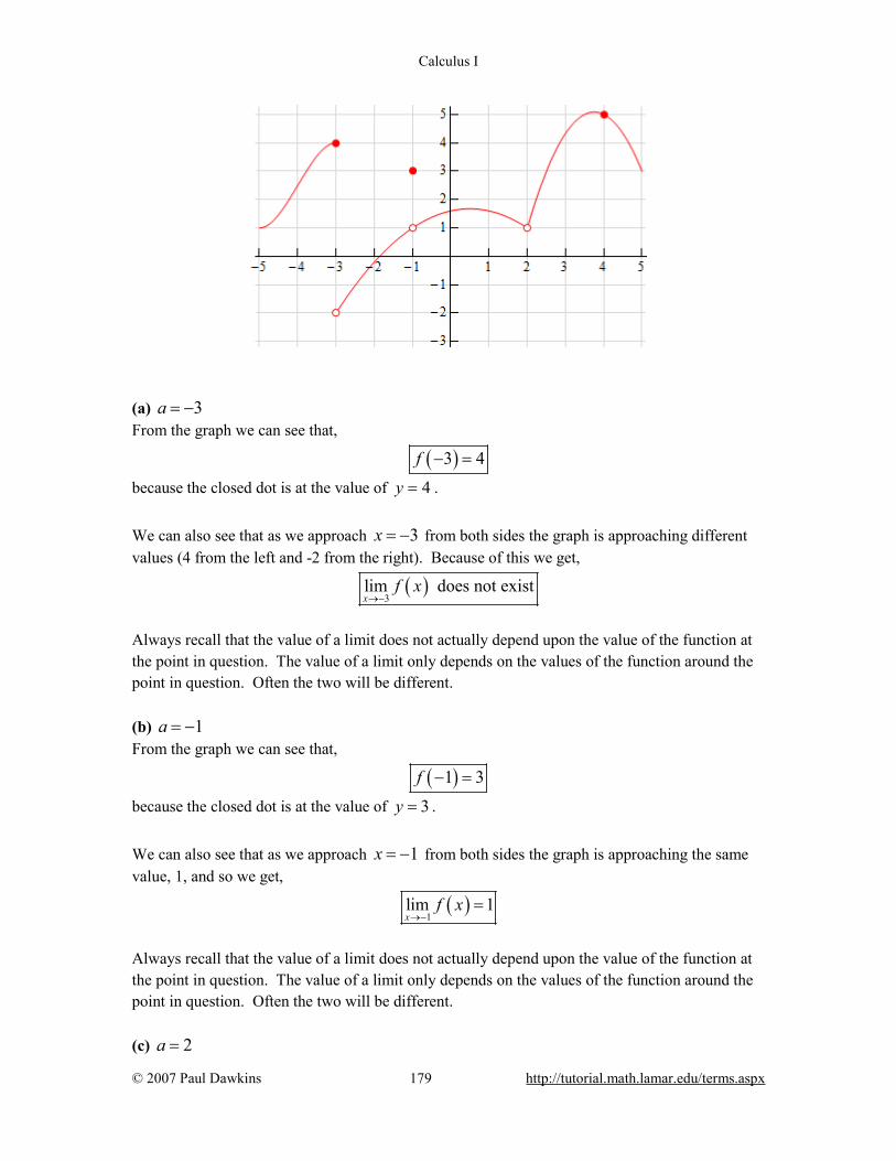
Calculus I
© 2007 Paul Dawkins 179 http://tutorial.math.lamar.edu/terms.aspx
(a) 3a = − From the graph we can see that,
( )3 4f − = because the closed dot is at the value of 4y = . We can also see that as we approach 3x = − from both sides the graph is approaching different values (4 from the left and -2 from the right). Because of this we get,
( )3
lim does not existx
f x→−
Always recall that the value of a limit does not actually depend upon the value of the function at the point in question. The value of a limit only depends on the values of the function around the point in question. Often the two will be different. (b) 1a = − From the graph we can see that,
( )1 3f − = because the closed dot is at the value of 3y = . We can also see that as we approach 1x = − from both sides the graph is approaching the same value, 1, and so we get,
( )1
lim 1x
f x→−
=
Always recall that the value of a limit does not actually depend upon the value of the function at the point in question. The value of a limit only depends on the values of the function around the point in question. Often the two will be different. (c) 2a =
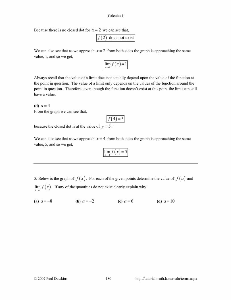
Calculus I
© 2007 Paul Dawkins 180 http://tutorial.math.lamar.edu/terms.aspx
Because there is no closed dot for 2x = we can see that,
( )2 does not existf We can also see that as we approach 2x = from both sides the graph is approaching the same value, 1, and so we get,
( )2
lim 1x
f x→
=
Always recall that the value of a limit does not actually depend upon the value of the function at the point in question. The value of a limit only depends on the values of the function around the point in question. Therefore, even though the function doesn’t exist at this point the limit can still have a value. (d) 4a = From the graph we can see that,
( )4 5f = because the closed dot is at the value of 5y = . We can also see that as we approach 4x = from both sides the graph is approaching the same value, 5, and so we get,
( )4
lim 5x
f x→
=
5. Below is the graph of ( )f x . For each of the given points determine the value of ( )f a and
( )limx a
f x→
. If any of the quantities do not exist clearly explain why.
(a) 8a = − (b) 2a = − (c) 6a = (d) 10a =

Calculus I
© 2007 Paul Dawkins 181 http://tutorial.math.lamar.edu/terms.aspx
(a) 8a = − From the graph we can see that,
( )8 3f − = − because the closed dot is at the value of 3y = − . We can also see that as we approach 8x = − from both sides the graph is approaching the same value, -6, and so we get,
( )8
lim 6x
f x→−
= −
Always recall that the value of a limit does not actually depend upon the value of the function at the point in question. The value of a limit only depends on the values of the function around the point in question. Often the two will be different. (b) 2a = − From the graph we can see that,
( )2 3f − = because the closed dot is at the value of 3y = . We can also see that as we approach 2x = − from both sides the graph is approaching different values (3 from the left and doesn’t approach any value from the right). Because of this we get,
( )2
lim does not existx
f x→−
Always recall that the value of a limit does not actually depend upon the value of the function at the point in question. The value of a limit only depends on the values of the function around the point in question. Often the two will be different. (c) 6a =

Calculus I
© 2007 Paul Dawkins 182 http://tutorial.math.lamar.edu/terms.aspx
From the graph we can see that,
( )6 5f = because the closed dot is at the value of 5y = . We can also see that as we approach 6x = from both sides the graph is approaching different values (2 from the left and 5 from the right). Because of this we get,
( )6
lim does not existx
f x→
Always recall that the value of a limit does not actually depend upon the value of the function at the point in question. The value of a limit only depends on the values of the function around the point in question. Often the two will be different. (d) 10a = From the graph we can see that,
( )10 0f = because the closed dot is at the value of 0y = . We can also see that as we approach 10x = from both sides the graph is approaching the same value, 0, and so we get,
( )10
lim 0x
f x→
=
6. Below is the graph of ( )f x . For each of the given points determine the value of ( )f a and
( )limx a
f x→
. If any of the quantities do not exist clearly explain why.
(a) 2a = − (b) 1a = − (c) 1a = (d) 3a =
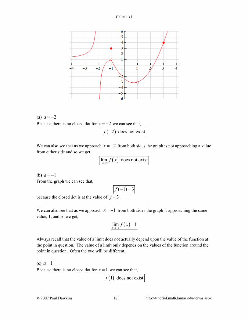
Calculus I
© 2007 Paul Dawkins 183 http://tutorial.math.lamar.edu/terms.aspx
(a) 2a = − Because there is no closed dot for 2x = − we can see that,
( )2 does not existf − We can also see that as we approach 2x = − from both sides the graph is not approaching a value from either side and so we get,
( )2
lim does not existx
f x→−
(b) 1a = − From the graph we can see that,
( )1 3f − = because the closed dot is at the value of 3y = . We can also see that as we approach 1x = − from both sides the graph is approaching the same value, 1, and so we get,
( )1
lim 1x
f x→−
=
Always recall that the value of a limit does not actually depend upon the value of the function at the point in question. The value of a limit only depends on the values of the function around the point in question. Often the two will be different. (c) 1a = Because there is no closed dot for 1x = we can see that,
( )1 does not existf

Calculus I
© 2007 Paul Dawkins 184 http://tutorial.math.lamar.edu/terms.aspx
We can also see that as we approach 1x = from both sides the graph is approaching the same value, -3, and so we get,
( )1
lim 3x
f x→
= −
Always recall that the value of a limit does not actually depend upon the value of the function at the point in question. The value of a limit only depends on the values of the function around the point in question. Therefore, even though the function doesn’t exist at this point the limit can still have a value. (d) 3a = From the graph we can see that,
( )3 4f = because the closed dot is at the value of 4y = . We can also see that as we approach 3x = from both sides the graph is approaching the same value, 4, and so we get,
( )3
lim 4x
f x→
=
One-Sided Limits 1. Below is the graph of ( )f x . For each of the given points determine the value of ( )f a ,
( )limx a
f x−→
, ( )limx a
f x+→
, and ( )limx a
f x→
. If any of the quantities do not exist clearly explain why.
(a) 4a = − (b) 1a = − (c) 2a = (d) 4a =
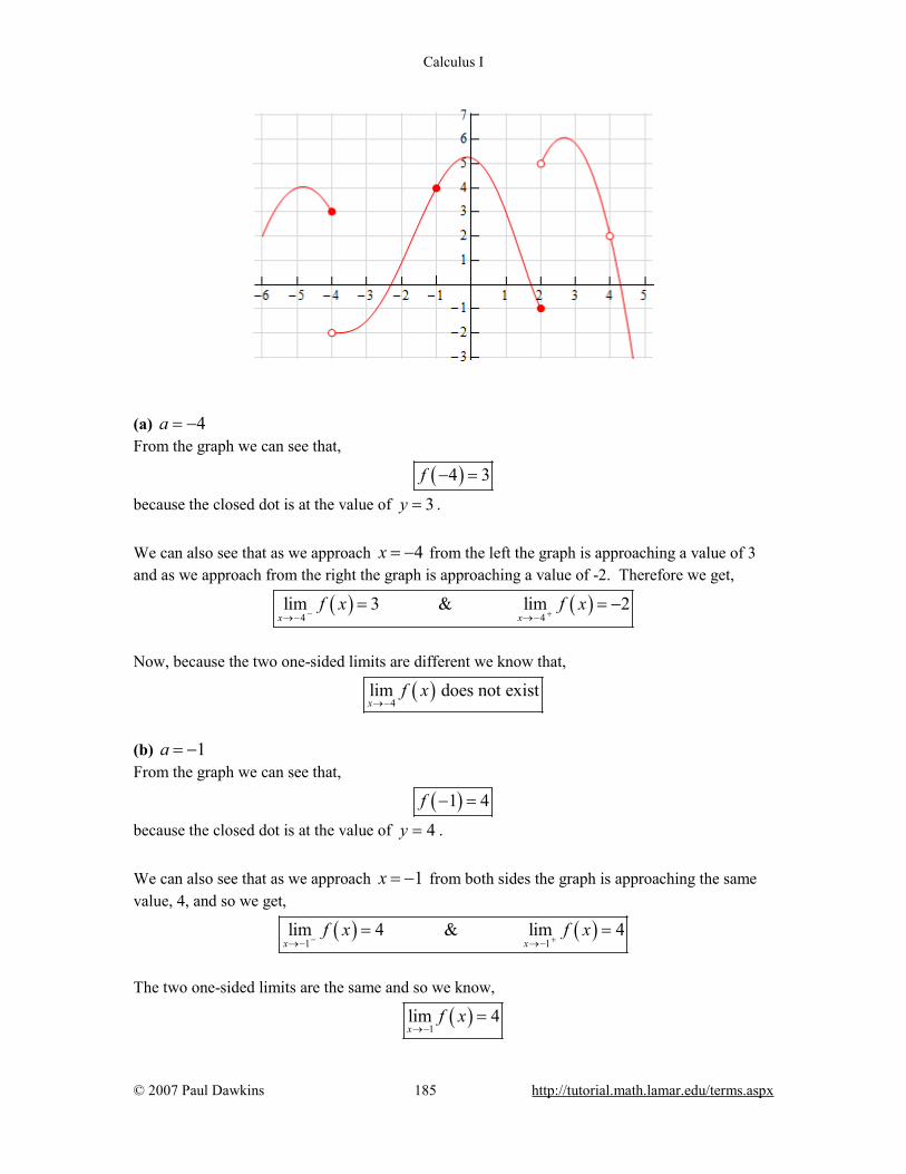
Calculus I
© 2007 Paul Dawkins 185 http://tutorial.math.lamar.edu/terms.aspx
(a) 4a = − From the graph we can see that,
( )4 3f − = because the closed dot is at the value of 3y = . We can also see that as we approach 4x = − from the left the graph is approaching a value of 3 and as we approach from the right the graph is approaching a value of -2. Therefore we get,
( ) ( )4 4
lim 3 & lim 2x x
f x f x− +→− →−
= = −
Now, because the two one-sided limits are different we know that,
( )4
lim does not existx
f x→−
(b) 1a = − From the graph we can see that,
( )1 4f − = because the closed dot is at the value of 4y = . We can also see that as we approach 1x = − from both sides the graph is approaching the same value, 4, and so we get,
( ) ( )1 1
lim 4 & lim 4x x
f x f x− +→− →−
= =
The two one-sided limits are the same and so we know,
( )1
lim 4x
f x→−
=

Calculus I
© 2007 Paul Dawkins 186 http://tutorial.math.lamar.edu/terms.aspx
(c) 2a = From the graph we can see that,
( )2 1f = − because the closed dot is at the value of 1y = − . We can also see that as we approach 2x = from the left the graph is approaching a value of -1 and as we approach from the right the graph is approaching a value of 5. Therefore we get,
( ) ( )2 2
lim 1 & lim 5x x
f x f x− +→ →
= − =
Now, because the two one-sided limits are different we know that,
( )2
lim does not existx
f x→
(d) 4a = Because there is no closed dot for 4x = we can see that,
( )4 does not existf We can also see that as we approach 4x = from both sides the graph is approaching the same value, 2, and so we get,
( ) ( )4 4
lim 2 & lim 2x x
f x f x− +→ →
= =
The two one-sided limits are the same and so we know,
( )4
lim 2x
f x→
=
Always recall that the value of a limit (including one-sided limits) does not actually depend upon the value of the function at the point in question. The value of a limit only depends on the values of the function around the point in question. Therefore, even though the function doesn’t exist at this point the limit and one-sided limits can still have a value. 2. Below is the graph of ( )f x . For each of the given points determine the value of ( )f a ,
( )limx a
f x−→
, ( )limx a
f x+→
, and ( )limx a
f x→
. If any of the quantities do not exist clearly explain why.
(a) 2a = − (b) 1a = (c) 3a = (d) 5a =
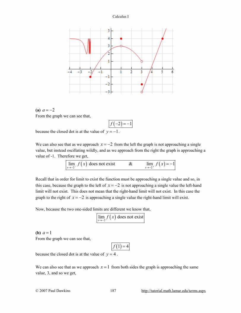
Calculus I
© 2007 Paul Dawkins 187 http://tutorial.math.lamar.edu/terms.aspx
(a) 2a = − From the graph we can see that,
( )2 1f − = − because the closed dot is at the value of 1y = − . We can also see that as we approach 2x = − from the left the graph is not approaching a single value, but instead oscillating wildly, and as we approach from the right the graph is approaching a value of -1. Therefore we get,
( ) ( )2 2
lim does not exist & lim 1x x
f x f x− +→− →−
= −
Recall that in order for limit to exist the function must be approaching a single value and so, in this case, because the graph to the left of 2x = − is not approaching a single value the left-hand limit will not exist. This does not mean that the right-hand limit will not exist. In this case the graph to the right of 2x = − is approaching a single value the right-hand limit will exist. Now, because the two one-sided limits are different we know that,
( )2
lim does not existx
f x→−
(b) 1a = From the graph we can see that,
( )1 4f = because the closed dot is at the value of 4y = . We can also see that as we approach 1x = from both sides the graph is approaching the same value, 3, and so we get,
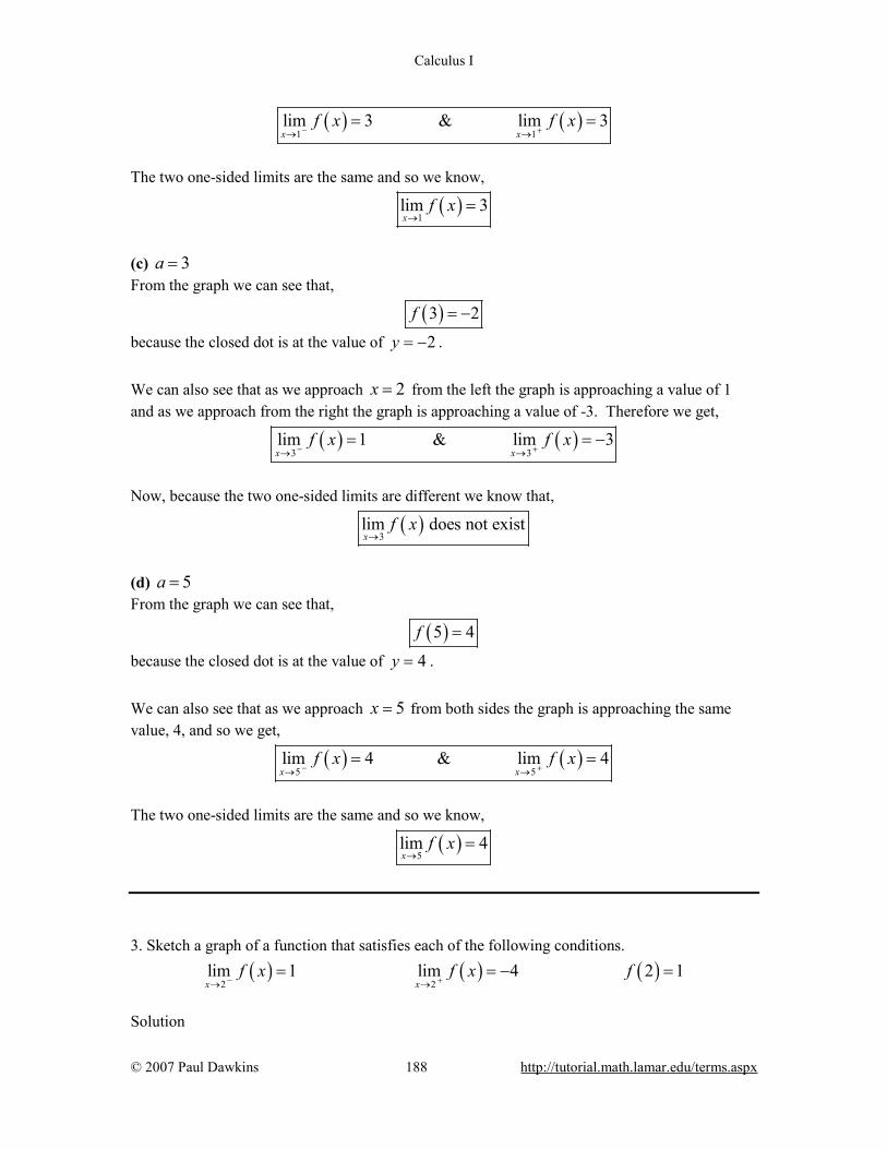
Calculus I
© 2007 Paul Dawkins 188 http://tutorial.math.lamar.edu/terms.aspx
( ) ( )1 1
lim 3 & lim 3x x
f x f x− +→ →
= =
The two one-sided limits are the same and so we know,
( )1
lim 3x
f x→
=
(c) 3a = From the graph we can see that,
( )3 2f = − because the closed dot is at the value of 2y = − . We can also see that as we approach 2x = from the left the graph is approaching a value of 1 and as we approach from the right the graph is approaching a value of -3. Therefore we get,
( ) ( )3 3
lim 1 & lim 3x x
f x f x− +→ →
= = −
Now, because the two one-sided limits are different we know that,
( )3
lim does not existx
f x→
(d) 5a = From the graph we can see that,
( )5 4f = because the closed dot is at the value of 4y = . We can also see that as we approach 5x = from both sides the graph is approaching the same value, 4, and so we get,
( ) ( )5 5
lim 4 & lim 4x x
f x f x− +→ →
= =
The two one-sided limits are the same and so we know,
( )5
lim 4x
f x→
=
3. Sketch a graph of a function that satisfies each of the following conditions. ( ) ( ) ( )
2 2lim 1 lim 4 2 1x x
f x f x f− +→ →
= = − =
Solution
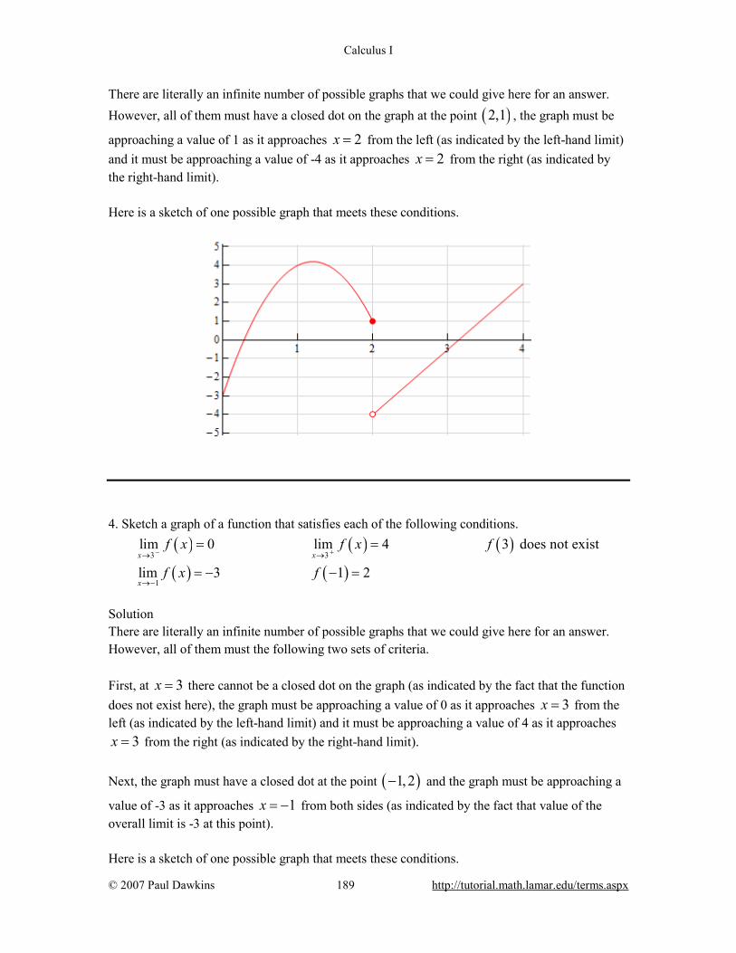
Calculus I
© 2007 Paul Dawkins 189 http://tutorial.math.lamar.edu/terms.aspx
There are literally an infinite number of possible graphs that we could give here for an answer. However, all of them must have a closed dot on the graph at the point ( )2,1 , the graph must be
approaching a value of 1 as it approaches 2x = from the left (as indicated by the left-hand limit) and it must be approaching a value of -4 as it approaches 2x = from the right (as indicated by the right-hand limit). Here is a sketch of one possible graph that meets these conditions.
4. Sketch a graph of a function that satisfies each of the following conditions.
( ) ( ) ( )( ) ( )
3 3
1
lim 0 lim 4 3 does not exist
lim 3 1 2x x
x
f x f x f
f x f− +→ →
→−
= =
= − − =
Solution There are literally an infinite number of possible graphs that we could give here for an answer. However, all of them must the following two sets of criteria. First, at 3x = there cannot be a closed dot on the graph (as indicated by the fact that the function does not exist here), the graph must be approaching a value of 0 as it approaches 3x = from the left (as indicated by the left-hand limit) and it must be approaching a value of 4 as it approaches
3x = from the right (as indicated by the right-hand limit). Next, the graph must have a closed dot at the point ( )1, 2− and the graph must be approaching a
value of -3 as it approaches 1x = − from both sides (as indicated by the fact that value of the overall limit is -3 at this point). Here is a sketch of one possible graph that meets these conditions.
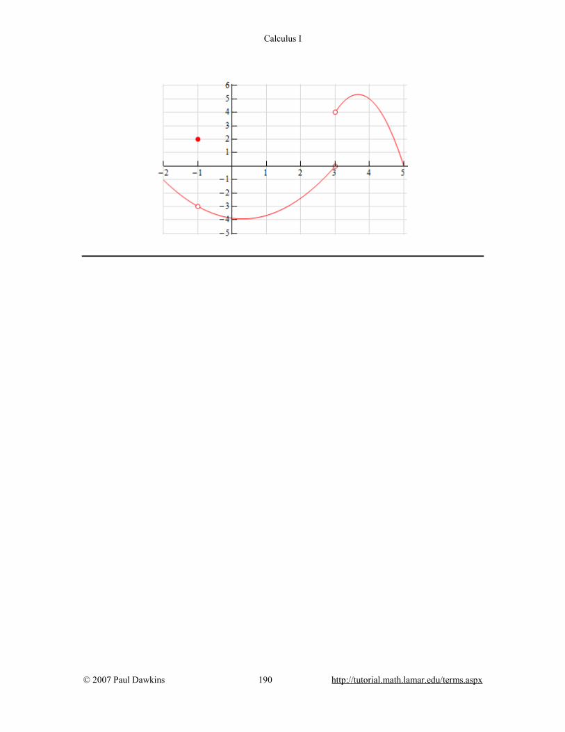
Calculus I
© 2007 Paul Dawkins 190 http://tutorial.math.lamar.edu/terms.aspx

Calculus I
© 2007 Paul Dawkins 191 http://tutorial.math.lamar.edu/terms.aspx
Limit Properties 1. Given ( )
8lim 9x
f x→
= − , ( )8
lim 2x
g x→
= and ( )8
lim 4x
h x→
= use the limit properties given in this
section to compute each of the following limits. If it is not possible to compute any of the limits clearly explain why not. (a) ( ) ( )
8lim 2 12x
f x h x→
− (b) ( )8
lim 3 6x
h x→
−
(c) ( ) ( ) ( )8
limx
g x h x f x→
− (d) ( ) ( ) ( )8
limx
f x g x h x→
− +
Hint : For each of these all we need to do is use the limit properties on the limit until the given limits appear and we can then compute the value.
(a) ( ) ( )8
lim 2 12x
f x h x→
−
Here is the work for this limit. At each step the property (or properties) used are listed and note that in some cases the properties may have been used more than once in the indicated step.
( ) ( ) ( ) ( )( ) ( )
( ) ( )
8 8 8
8 8
lim 2 12 lim 2 lim 12 Property 2
2lim 12lim Property 1
2 9 12 4 Plug in values of limits
66
x x x
x x
f x h x f x h x
f x h x→ → →
→ →
− = −
= −
= − −
= −
(b) ( )8
lim 3 6x
h x→
−
Here is the work for this limit. At each step the property (or properties) used are listed and note that in some cases the properties may have been used more than once in the indicated step.
( ) ( )( )
( )
8 8 8
8 8
lim 3 6 lim 3 lim 6 Property 2
3lim lim6 Property 1
3 4 6 Plug in value of limits & Property 7
6
x x x
x x
h x h x
h x→ → →
→ →
− = −
= −
= −
=
(c) ( ) ( ) ( )8
limx
g x h x f x→
−
Calculus I
© 2007 Paul Dawkins 192 http://tutorial.math.lamar.edu/terms.aspx
Here is the work for this limit. At each step the property (or properties) used are listed and note that in some cases the properties may have been used more than once in the indicated step.
( ) ( ) ( ) ( ) ( ) ( )
( ) ( ) ( )
( )( ) ( )
8 8 8
8 8 8
lim lim lim Property 2
lim lim lim Property 3
2 4 9 Plug in values of limits
17
x x x
x x x
g x h x f x g x h x f x
g x h x f x
→ → →
→ → →
− = −
= − = − −
=
(d) ( ) ( ) ( )8
limx
f x g x h x→
− +
Here is the work for this limit. At each step the property (or properties) used are listed and note that in some cases the properties may have been used more than once in the indicated step.
( ) ( ) ( ) ( ) ( ) ( )8 8 8 8
lim lim lim lim Property 2
9 2 4 Plug in values of limits
7
x x x xf x g x h x f x g x h x
→ → → →− + = − +
= − − +
= −
2. Given ( )
4lim 1x
f x→−
= , ( )4
lim 10x
g x→−
= and ( )4
lim 7x
h x→−
= − use the limit properties given in
this section to compute each of the following limits. If it is not possible to compute any of the limits clearly explain why not.
(a) ( )( )
( )( )4
limx
f x h xg x f x→−
−
(b) ( ) ( ) ( )
4limx
f x g x h x→−
(c) ( )
( )( ) ( )4
31limx
f xh x g x h x→−
−+ +
(d) ( ) ( ) ( )4
1lim 27x
h xh x f x→−
− +
Hint : For each of these all we need to do is use the limit properties on the limit until the given limits appear and we can then compute the value.
(a) ( )( )
( )( )4
limx
f x h xg x f x→−
−
Here is the work for this limit. At each step the property (or properties) used are listed and note that in some cases the properties may have been used more than once in the indicated step.
Calculus I
© 2007 Paul Dawkins 193 http://tutorial.math.lamar.edu/terms.aspx
( )( )
( )( )
( )( )
( )( )
( )( )
( )( )
4 4 4
4 4
4 4
lim lim lim Property 2
lim limProperty 4
lim lim
1 7 Plug in values of limits10 17110
x x x
x x
x x
f x h x f x h xg x f x g x f x
f x h x
g x f x
→− →− →−
→− →−
→− →−
− = −
= −
−= −
=
Note that were able to use Property 4 in the second step only because after we evaluated the limit of the denominators (both of them) we found that the limits of the denominators were not zero.
(b) ( ) ( ) ( )4
limx
f x g x h x→−
Here is the work for this limit. At each step the property (or properties) used are listed and note that in some cases the properties may have been used more than once in the indicated step.
( ) ( ) ( ) ( ) ( ) ( )
( )( ) ( )4 4 4 4
lim lim lim lim Property 3
1 10 7 Plug in value of limits
70
x x x xf x g x h x f x g x h x
→− →− →− →− =
= −
= −
Note that the properties 2 & 3 in this section were only given with two functions but they can easily be extended out to more than two functions as we did here for property 3.
(c) ( )
( )( ) ( )4
31limx
f xh x g x h x→−
−+ +
Here is the work for this limit. At each step the property (or properties) used are listed and note that in some cases the properties may have been used more than once in the indicated step.

Calculus I
© 2007 Paul Dawkins 194 http://tutorial.math.lamar.edu/terms.aspx
( )( )
( ) ( ) ( )( )
( ) ( )
( )( )
( ) ( )
( )( )
( ) ( )
4 4 4
4 4
4 4
4 4 4
4 4 4
3 31 1lim lim lim Property 2
lim 1 lim 3Property 4
lim lim
lim 1 lim 3 limProperty 2
lim lim lim
1 3 17 10
x x x
x x
x x
x x x
x x x
f x f xh x g x h x h x g x h x
f x
h x g x h x
f x
h x g x h x
→− →− →−
→− →−
→− →−
→− →− →−
→− →− →−
− −+ = + + +
− = +
+
−= +
+
−= +
−Plug in values of limits
7& Property 1
1121
−
=
Note that were able to use Property 4 in the second step only because after we evaluated the limit of the denominators (both of them) we found that the limits of the denominators were not zero.
(d) ( ) ( ) ( )4
1lim 27x
h xh x f x→−
− +
Here is the work for this limit. At each step the property (or properties) used are listed and note that in some cases the properties may have been used more than once in the indicated step.
( ) ( ) ( ) ( ) ( ) ( )
( ) ( ) ( )
4 4 4
4
44
1 1lim 2 lim 2 lim Property 27 7
lim 1lim 2 Property 4
lim 7
x x x
xx
x
h x h xh x f x h x f x
h xh x f x
→− →− →−
→−
→−→−
− = − + +
= −+
At this point let’s step back a minute. In the previous parts we didn’t worry about using property 4 on a rational expression. However, in this case let’s be a little more careful. We can only use property 4 if the limit of the denominator is not zero. Let’s check that limit and see what we get.
( ) ( ) ( ) ( )( ) ( )( )
4 4 4
4 4
lim 7 lim lim 7 Property 2
lim 7 lim Property 1
7 7 1 Plug in values of limits & Property 10
x x x
x x
h x f x h x f x
h x f x→− →− →−
→− →−
+ = +
= +
= − +
=
Okay, we can see that the limit of the denominator in the second term will be zero and so we can not actually use property 4 on that term. This means that this limit cannot be done and note that
Calculus I
© 2007 Paul Dawkins 195 http://tutorial.math.lamar.edu/terms.aspx
the fact that we could determine a value for the limit of the first term will not change this fact. This limit cannot be done. 3. Given ( )
0lim 6x
f x→
= , ( )0
lim 4x
g x→
= − and ( )0
lim 1x
h x→
= − use the limit properties given in this
section to compute each of the following limits. If it is not possible to compute any of the limits clearly explain why not.
(a) ( ) ( ) 3
0limx
f x h x→
+ (b) ( ) ( )0
limx
g x h x→
(c) ( ) 230
lim 11x
g x→
+ (d) ( )
( ) ( )0limx
f xh x g x→ −
Hint : For each of these all we need to do is use the limit properties on the limit until the given limits appear and we can then compute the value.
(a) ( ) ( ) 3
0limx
f x h x→
+
Here is the work for this limit. At each step the property (or properties) used are listed and note that in some cases the properties may have been used more than once in the indicated step.
( ) ( ) ( ) ( )( )
( ) ( )
[ ]
33
0 0
3
0 0
3
lim lim Property 5
lim lim Property 2
6 1 Plug in values of limits
125
x x
x x
f x h x f x h x
f x h x
→ →
→ →
+ = +
= +
= −
=
(b) ( ) ( )0
limx
g x h x→
Here is the work for this limit. At each step the property (or properties) used are listed and note that in some cases the properties may have been used more than once in the indicated step.
( ) ( ) ( ) ( )
( ) ( )
( ) ( )
0 0
0 0
lim lim Property 6
lim lim Property 3
4 1 Plug in value of limits
2
x x
x x
g x h x g x h x
g x h x
→ →
→ →
=
=
= − −
=

Calculus I
© 2007 Paul Dawkins 196 http://tutorial.math.lamar.edu/terms.aspx
(c) ( ) 23
0lim 11x
g x→
+
Here is the work for this limit. At each step the property (or properties) used are listed and note that in some cases the properties may have been used more than once in the indicated step.
( ) ( )( )( )
( )
( )
2 23 30 0
23
0 0
23
0 0
23
lim 11 lim 11 Property 6
lim11 lim Property 2
lim11 lim Property 5
11 4 Plug in values of limits & Property 7
3
x x
x x
x x
g x g x
g x
g x
→ →
→ →
→ →
+ = +
= +
= +
= + −
=
(d) ( )
( ) ( )0limx
f xh x g x→ −
Here is the work for this limit. At each step the property (or properties) used are listed and note that in some cases the properties may have been used more than once in the indicated step.
( )( ) ( )
( )( ) ( )
( )( ) ( )( )
( )( ) ( )
( )
0 0
0
0
0
0 0
lim lim Property 6
limProperty 4
lim
limProperty 2
lim lim
6 Plug in values of limits 1 4
2
x x
x
x
x
x x
f x f xh x g x h x g x
f x
h x g x
f x
h x g x
→ →
→
→
→
→ →
=− −
=−
=−
=− − −
=
Note that were able to use Property 4 in the second step only because after we evaluated the limit of the denominators (both of them) we found that the limits of the denominators were not zero. 4. Use the limit properties given in this section to compute the following limit. At each step clearly indicate the property being used. If it is not possible to compute any of the limits clearly explain why not.

Calculus I
© 2007 Paul Dawkins 197 http://tutorial.math.lamar.edu/terms.aspx
( )3
2lim 14 6t
t t→−
− +
Hint : All we need to do is use the limit properties on the limit until we can use Properties 7, 8 and/or 9 from this section to compute the limit.
( )
( ) ( )
3 3
2 2 2 2
3
2 2 2
3
lim 14 6 lim14 lim 6 lim Property 2
lim14 6 lim lim Property 1
14 6 2 2 Properties 7, 8, & 9
18
t t t t
t t t
t t t t
t t→− →− →− →−
→− →− →−
− + = − +
= − +
= − − + −
=
5. Use the limit properties given in this section to compute the following limit. At each step clearly indicate the property being used. If it is not possible to compute any of the limits clearly explain why not.
( )2
6lim 3 7 16x
x x→
+ −
Hint : All we need to do is use the limit properties on the limit until we can use Properties 7, 8 and/or 9 from this section to compute the limit.
( )
( ) ( )
2 2
6 6 6 62
6 6 6
2
lim 3 7 16 lim3 lim 7 lim16 Property 2
3lim 7 lim lim16 Property 1
3 6 7 6 16 Properties 7, 8, & 9
134
x x x x
x x x
x x x x
x x→ → → →
→ → →
+ − = + −
= + −
= + −
=
6. Use the limit properties given in this section to compute the following limit. At each step clearly indicate the property being used. If it is not possible to compute any of the limits clearly explain why not.
2
3
8lim4 7w
w ww→
−−
Hint : All we need to do is use the limit properties on the limit until we can use Properties 7, 8 and/or 9 from this section to compute the limit.

Calculus I
© 2007 Paul Dawkins 198 http://tutorial.math.lamar.edu/terms.aspx
( )( )
( )( )
223
33
2
3 3
3 32
3 3
3 32
lim 88lim Property 44 7 lim 4 7
lim lim8Property 2
lim 4 lim 7
lim 8limProperty 1
lim 4 7 lim
3 8 3Properties 7, 8, & 9
4 7 3
1517
ww
w
w w
w w
w w
w w
w ww ww w
w w
w
w w
w
→
→→
→ →
→ →
→ →
→ →
−−=
− −
−=
−
−=
−
−=
−
=
Note that we were able to use property 4 in the first step because after evaluating the limit in the denominator we found that it wasn’t zero. 7. Use the limit properties given in this section to compute the following limit. At each step clearly indicate the property being used. If it is not possible to compute any of the limits clearly explain why not.
25
7lim3 10x
xx x→−
++ −
Hint : All we need to do is use the limit properties on the limit until we can use Properties 7, 8 and/or 9 from this section to compute the limit.
( )
( )5
2 255
lim 77lim Property 43 10 lim 3 10
x
xx
xxx x x x
→−
→−→−
++=
+ − + −
Okay, at this point let’s step back a minute. We used property 4 here and we know that we can only do that if the limit of the denominator is not zero. So, let’s check that out and see what we get.
( )
( ) ( )
2 2
5 5 5 5
2
5 5 5
2
lim 3 10 lim lim 3 lim 10 Property 2
lim 3 lim lim 10 Property 1
5 3 5 10 Properties 7, 8, & 90
x x x x
x x x
x x x x
x x→− →− →− →−
→− →− →−
+ − = + −
= + −
= − + − −
=
Calculus I
© 2007 Paul Dawkins 199 http://tutorial.math.lamar.edu/terms.aspx
So, the limit of the denominator is zero and so we couldn’t use property 4 in this case. Therefore, we cannot do this limit at this point (note that it will be possible to do this limit after the next section). 8. Use the limit properties given in this section to compute the following limit. At each step clearly indicate the property being used. If it is not possible to compute any of the limits clearly explain why not.
2
0lim 6z
z→
+
Hint : All we need to do is use the limit properties on the limit until we can use Properties 7, 8 and/or 9 from this section to compute the limit.
( )2 2
0 0
2
0 0
2
lim 6 lim 6 Property 6
lim lim 6 Property 2
0 6 Properties 7 & 9
6
z z
z z
z z
z
→ →
→ →
+ = +
= +
= +
=
9. Use the limit properties given in this section to compute the following limit. At each step clearly indicate the property being used. If it is not possible to compute any of the limits clearly explain why not.
( )3
10lim 4 2x
x x→
+ −
Hint : All we need to do is use the limit properties on the limit until we can use Properties 7, 8 and/or 9 from this section to compute the limite.
( )( )
( )
3 3
10 10 10
310 10
310 10 10
310 10 10
3
lim 4 2 lim 4 lim 2 Property 2
lim 4 lim 2 Property 6
lim 4 lim lim 2 Property 2
4 lim lim lim 2 Property 1
4 10 10 2 Properties 7 & 842
x x x
x x
x x x
x x x
x x x x
x x
x x
x x
→ → →
→ →
→ → →
→ → →
+ − = + −
= + −
= + −
= + −
= + −
=
Calculus I
© 2007 Paul Dawkins 200 http://tutorial.math.lamar.edu/terms.aspx
Computing Limits
1. Evaluate ( )2
2lim 8 3 12x
x x→
− + , if it exists.
Solution There is not really a lot to this problem. Simply recall the basic ideas for computing limits that we looked at in this section. We know that the first thing that we should try to do is simply plug in the value and see if we can compute the limit.
( ) ( ) ( )2
2lim 8 3 12 8 3 2 12 4 50x
x x→
− + = − + =
2. Evaluate 23
6 4lim1t
tt→−
++
, if it exists.
Solution There is not really a lot to this problem. Simply recall the basic ideas for computing limits that we looked at in this section. We know that the first thing that we should try to do is simply plug in the value and see if we can compute the limit.
23
6 4 6 3lim1 10 5t
tt→−
+ −= = −
+
3. Evaluate 2
25
25lim2 15x
xx x→−
−+ −
, if it exists.
Solution There is not really a lot to this problem. Simply recall the basic ideas for computing limits that we looked at in this section. In this case we see that if we plug in the value we get 0/0. Recall that this DOES NOT mean that the limit doesn’t exist. We’ll need to do some more work before we make that conclusion. All we need to do here is some simplification and then we’ll reach a point where we can plug in the value.

Calculus I
© 2007 Paul Dawkins 201 http://tutorial.math.lamar.edu/terms.aspx
( )( )( )( )
2
25 5 5
5 525 5 5lim lim lim2 15 3 5 3 4x x x
x xx xx x x x x→− →− →−
− +− −= = =
+ − − + −
4. Evaluate 2
8
2 17 8lim8z
z zz→
− +−
, if it exists.
Solution There is not really a lot to this problem. Simply recall the basic ideas for computing limits that we looked at in this section. In this case we see that if we plug in the value we get 0/0. Recall that this DOES NOT mean that the limit doesn’t exist. We’ll need to do some more work before we make that conclusion. All we need to do here is some simplification and then we’ll reach a point where we can plug in the value.
( )( )
( )2
8 8 8
2 1 82 17 8 2 1lim lim lim 158 8 1z z z
z zz z zz z→ → →
− −− + −= = = −
− − − −
5. Evaluate 2
27
4 21lim3 17 28y
y yy y→
− −− −
, if it exists.
Solution There is not really a lot to this problem. Simply recall the basic ideas for computing limits that we looked at in this section. In this case we see that if we plug in the value we get 0/0. Recall that this DOES NOT mean that the limit doesn’t exist. We’ll need to do some more work before we make that conclusion. All we need to do here is some simplification and then we’ll reach a point where we can plug in the value.
( )( )
( )( )2
27 7 7
7 34 21 3 10 2lim lim lim3 17 28 3 4 7 3 4 25 5y y y
y yy y yy y y y y→ → →
− +− − += = = =
− − + − +
6. Evaluate ( )2
0
6 36limh
hh→
+ −, if it exists.
Solution There is not really a lot to this problem. Simply recall the basic ideas for computing limits that we looked at in this section. In this case we see that if we plug in the value we get 0/0. Recall that this DOES NOT mean that the limit doesn’t exist. We’ll need to do some more work before
Calculus I
© 2007 Paul Dawkins 202 http://tutorial.math.lamar.edu/terms.aspx
we make that conclusion. All we need to do here is some simplification and then we’ll reach a point where we can plug in the value.
( ) ( ) ( )2 2
0 0 0 0
6 36 1236 12 36lim lim lim lim 12 12h h h h
h h hh h hh h h→ → → →
+ − ++ + −= = = + =
7. Evaluate 4
2lim4z
zz→
−−
, if it exists.
Solution There is not really a lot to this problem. Simply recall the basic ideas for computing limits that we looked at in this section. In this case we see that if we plug in the value we get 0/0. Recall that this DOES NOT mean that the limit doesn’t exist. We’ll need to do some more work before we make that conclusion. If you’re really good at factoring you can factor this and simplify. Another method that can be used however is to rationalize the numerator, so let’s do that for this problem.
( )( )
( )( ) ( )( )4 4 4 4
2 22 4 1 1lim lim lim lim4 4 422 4 2z z z z
z zz zz z zz z z→ → → →
− +− −= = = =
− − ++ − +
8. Evaluate 3
2 22 4lim3x
xx→−
+ −+
, if it exists.
Solution There is not really a lot to this problem. Simply recall the basic ideas for computing limits that we looked at in this section. In this case we see that if we plug in the value we get 0/0. Recall that this DOES NOT mean that the limit doesn’t exist. We’ll need to do some more work before we make that conclusion. Simply factoring will not do us much good here so in this case it looks like we’ll need to rationalize the numerator.
( )( )
( )( ) ( )( )
( )( )( )
3 3 3
3 3
2 22 4 2 22 42 22 4 2 22 16lim lim lim3 3 2 22 4 3 2 22 4
2 3 2 2 1lim lim8 42 22 43 2 22 4
x x x
x x
x xx xx x x x x
xxx x
→− →− →−
→− →−
+ − + ++ − + −= =
+ + + + + + +
+= = = =
+ ++ + +

Calculus I
© 2007 Paul Dawkins 203 http://tutorial.math.lamar.edu/terms.aspx
9. Evaluate 0
lim3 9x
xx→ − +
, if it exists.
Solution There is not really a lot to this problem. Simply recall the basic ideas for computing limits that we looked at in this section. In this case we see that if we plug in the value we get 0/0. Recall that this DOES NOT mean that the limit doesn’t exist. We’ll need to do some more work before we make that conclusion. Simply factoring will not do us much good here so in this case it looks like we’ll need to rationalize the denominator.
( )( )( )
( )( )
( )0 0 0
0 0
3 9 3 9lim lim lim
9 93 9 3 9 3 9
3 9 3 9lim lim 61
x x x
x x
x x xx xxx x x
x x xx
→ → →
→ →
+ + + += =
− +− + − + + +
+ + + += = = −
− −
10. Given the function
( ) 2
7 4 12 1x x
f xx x
− <= + ≥
Evaluate the following limits, if they exist. (a) ( )
6limx
f x→−
(b) ( )1
limx
f x→
Hint : Recall that when looking at overall limits (as opposed to one-sided limits) we need to make sure that the value of the function must be approaching the same value from both sides. In other words, the two one sided limits must both exist and be equal. (a) ( )
6limx
f x→−
Solution
For this part we know that 6 1− < and so there will be values of x on both sides of -6 in the range 1x < and so we can assume that, in the limit, we will have 1x < . This will allow us to use the
piece of the function in that range and then just use standard limit techniques to compute the limit.
( ) ( )6 6
lim lim 7 4 31x x
f x x→− →−
= − =
(b) ( )
1limx
f x→
Solution
This part is going to be different from the previous part. We are looking at the limit at 1x = and that is the “cut–off” point in the piecewise functions. Recall from the discussion in the section, that this means that we are going to have to look at the two one sided limits.

Calculus I
© 2007 Paul Dawkins 204 http://tutorial.math.lamar.edu/terms.aspx
( ) ( )
1 1lim lim 7 4 3 because 1 implies that 1x x
f x x x x− −
−
→ →= − = → <
( ) ( )2
1 1lim lim 2 3 because 1 implies that 1x x
f x x x x+ +
+
→ →= + = → >
So, in this case, we can see that, ( ) ( )
1 1lim lim 3x x
f x f x− +→ →
= =
and so we know that the overall limit must exist and,
( )1
lim 3x
f x→
=
11. Given the function
( ) 6 41 9 4
z zh z
z z≤ −
= − > −
Evaluate the following limits, if they exist. (a) ( )
7limz
h z→
(b) ( )4
limz
h z→−
Hint : Recall that when looking at overall limits (as opposed to one-sided limits) we need to make sure that the value of the function must be approaching the same value from both sides. In other words, the two one sided limits must both exist and be equal. (a) ( )
7limz
h z→
Solution
For this part we know that 7 4> − and so there will be values of z on both sides of 7 in the range 4z > − and so we can assume that, in the limit, we will have 4z > − . This will allow us to use
the piece of the function in that range and then just use standard limit techniques to compute the limit.
( ) ( )7 7
lim lim 1 9 62z z
h z z→ →
= − = −
(b) ( )
4limz
h z→−
Solution
This part is going to be different from the previous part. We are looking at the limit at 4z = − and that is the “cut–off” point in the piecewise functions. Recall from the discussion in the section, that this means that we are going to have to look at the two one sided limits. ( )
4 4lim lim 6 24 because 4 implies that 4
z zh z z z z
− −
−
→− →−= = − → − < −
( ) ( )4 4
lim lim 1 9 37 because 4 implies that 4z z
h z z z z+ +
+
→− →−= − = → − > −
Calculus I
© 2007 Paul Dawkins 205 http://tutorial.math.lamar.edu/terms.aspx
So, in this case, we can see that, ( ) ( )
4 4lim 24 37 lim
z zh z h z
− +→− →−= − ≠ =
and so we know that the overall limit does not exist.
12. Evaluate ( )5
lim 10 5x
x→
+ − , if it exists.
Hint : Recall the mathematical definition of the absolute value function and that it is in fact a piecewise function. Solution Recall the definition of the absolute value function.
00
p pp
p p≥
= − <
So, because the function inside the absolute value is zero at 5x = we can see that,
( )5 5
55 5
x xx
x x− ≥
− = − − <
This means that we are being asked to compute the limit at the “cut–off” point in a piecewise function and so, as we saw in this section, we’ll need to look at two one-sided limits in order to determine if this limit exists (and its value if it does exist).
( ) ( )( ) ( )5 5 5
lim 10 5 lim 10 5 lim 15 10 recall 5 implies 5x x x
x x x x x− − −
−
→ → →+ − = − − = − = → <
( ) ( )( ) ( )5 5 5
lim 10 5 lim 10 5 lim 5 10 recall 5 implies 5x x x
x x x x x+ + −
+
→ → →+ − = + − = + = → >
So, for this problem, we can see that,
( ) ( )55
lim 10 5 lim 10 5 10xx
x x− → +→
+ − = + − =
and so the overall limit must exist and,
( )5
lim 10 5 10x
x−→
+ − =
13. Evaluate 1
1lim1t
tt→−
++
, if it exists.
Hint : Recall the mathematical definition of the absolute value function and that it is in fact a piecewise function.
Calculus I
© 2007 Paul Dawkins 206 http://tutorial.math.lamar.edu/terms.aspx
Solution Recall the definition of the absolute value function.
00
p pp
p p≥
= − <
So, because the function inside the absolute value is zero at 1t = − we can see that,
( )1 1
11 1
t tt
t t+ ≥ −
+ = − + < −
This means that we are being asked to compute the limit at the “cut–off” point in a piecewise function and so, as we saw in this section, we’ll need to look at two one-sided limits in order to determine if this limit exists (and its value if it does exist).
( )1 1 1
1 1lim lim lim 1 1 recall 1 implies 11 1t t t
t t t tt t− − −
−
→− →− →−
+ += = − = − → − < −
+ − +
1 1 1
1 1lim lim lim 1 1 recall 1 implies 11 1t t t
t t t tt t+ + +
+
→− →− →−
+ += = = → − > −
+ +
So, for this problem, we can see that,
1 1
1 1lim 1 1 lim1 1t t
t tt t− +→− →−
+ += − ≠ =
+ +
and so the overall limit does not exist. 14. Given that ( ) 27 3 2x f x x≤ ≤ + for all x determine the value of ( )
2limx
f x→
.
Hint : Recall the Squeeze Theorem. Solution This problem is set up to use the Squeeze Theorem. First, we already know that ( )f x is always
between two other functions. Now all that we need to do is verify that the two “outer” functions have the same limit at 2x = and if they do we can use the Squeeze Theorem to get the answer.
( )2
2 2lim 7 14 lim 3 2 14x x
x x→ →
= + =
So, we have,
( )2
2 2lim 7 lim 3 2 14x x
x x→ →
= + =
and so by the Squeeze Theorem we must also have,

Calculus I
© 2007 Paul Dawkins 207 http://tutorial.math.lamar.edu/terms.aspx
( )2
lim 14x
f x→
=
15. Use the Squeeze Theorem to determine the value of 4
0lim sinx
xxπ
→
.
Hint : Recall how we worked the Squeeze Theorem problem in this section to find the lower and upper functions we need in order to use the Squeeze Theorem. Solution We first need to determine lower/upper functions. We’ll start off by acknowledging that provided 0x ≠ (which we know it won’t be because we are looking at the limit as 0x → ) we will have,
1 sin 1xπ − ≤ ≤
Now, simply multiply through this by 4x to get,
4 4 4sinx x xxπ − ≤ ≤
Before proceeding note that we can only do this because we know that 4 0x > for 0x ≠ . Recall that if we multiply through an inequality by a negative number we would have had to switch the signs. So, for instance, had we multiplied through by 3x we would have had issues because this is positive if 0x > and negative if 0x < . Now, let’s get back to the problem. We have a set of lower/upper functions and clearly,
( )4 4
0 0lim lim 0x x
x x→ →
= − =
Therefore, by the Squeeze Theorem we must have,
4
0lim sin 0x
xxπ
→
=
Infinite Limits

Calculus I
© 2007 Paul Dawkins 208 http://tutorial.math.lamar.edu/terms.aspx
1. For ( )( )5
93
f xx
=−
evaluate the indicated limits, if they exist.
(a) ( )
3limx
f x−→
(b) ( )3
limx
f x+→
(c) ( )3
limx
f x→
(a) ( )
3limx
f x−→
Let’s start off by acknowledging that for 3x −→ we know 3x < . For the numerator we can see that, in the limit, it will just be 9. The denominator takes a little more work. Clearly, in the limit, we have,
3 0x − → but we can actually go a little farther. Because we know that 3x < we also know that, 3 0x − < More compactly, we can say that in the limit we will have, 3 0x −− → Raising this to the fifth power will not change this behavior and so, in the limit, the denominator will be,
( )53 0x −− → We can now do the limit of the function. In the limit, the numerator is a fixed positive constant and the denominator is an increasingly small negative number. In the limit, the quotient must then be an increasing large negative number or,
( )53
9lim3x x−→
= −∞−
Note that this also means that there is a vertical asymptote at 3x = . (b) ( )
3limx
f x+→
Let’s start off by acknowledging that for 3x +→ we know 3x > . As in the first part the numerator, in the limit, it will just be 9. The denominator will also work similarly to the first part. In the limit, we have,
3 0x − → and because we know that 3x > we also know that,
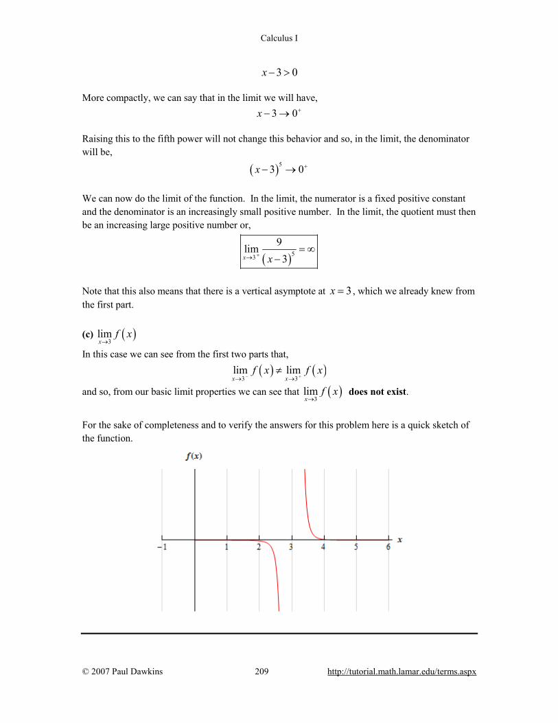
Calculus I
© 2007 Paul Dawkins 209 http://tutorial.math.lamar.edu/terms.aspx
3 0x − > More compactly, we can say that in the limit we will have, 3 0x +− → Raising this to the fifth power will not change this behavior and so, in the limit, the denominator will be,
( )53 0x +− → We can now do the limit of the function. In the limit, the numerator is a fixed positive constant and the denominator is an increasingly small positive number. In the limit, the quotient must then be an increasing large positive number or,
( )53
9lim3x x+→
= ∞−
Note that this also means that there is a vertical asymptote at 3x = , which we already knew from the first part. (c) ( )
3limx
f x→
In this case we can see from the first two parts that, ( ) ( )
3 3lim limx x
f x f x− +→ →
≠
and so, from our basic limit properties we can see that ( )3
limx
f x→
does not exist.
For the sake of completeness and to verify the answers for this problem here is a quick sketch of the function.
Calculus I
© 2007 Paul Dawkins 210 http://tutorial.math.lamar.edu/terms.aspx
2. For ( ) 26
th tt
=+
evaluate the indicated limits, if they exist.
(a) ( )
6lim
th t
−→− (b) ( )
6lim
th t
+→− (c) ( )
6limt
h t→−
(a) ( )
6lim
th t
−→−
Let’s start off by acknowledging that for 6t −→ − we know 6t < − . For the numerator we can see that, in the limit, we will get -12. The denominator takes a little more work. Clearly, in the limit, we have,
6 0t+ → but we can actually go a little farther. Because we know that 6t < − we also know that, 6 0t+ < More compactly, we can say that in the limit we will have, 6 0t −+ → So, in the limit, the numerator is approaching a negative number and the denominator is an increasingly small negative number. The quotient must then be an increasing large positive number or,
6
2lim6t
tt−→−
= ∞+
Note that this also means that there is a vertical asymptote at 6t = − . (b) ( )
6lim
th t
+→−
Let’s start off by acknowledging that for 6t +→ − we know 6t > − . For the numerator we can see that, in the limit, we will get -12. The denominator will also work similarly to the first part. In the limit, we have,
6 0t+ → but we can actually go a little farther. Because we know that 6t > − we also know that, 6 0t+ > More compactly, we can say that in the limit we will have, 6 0t ++ →
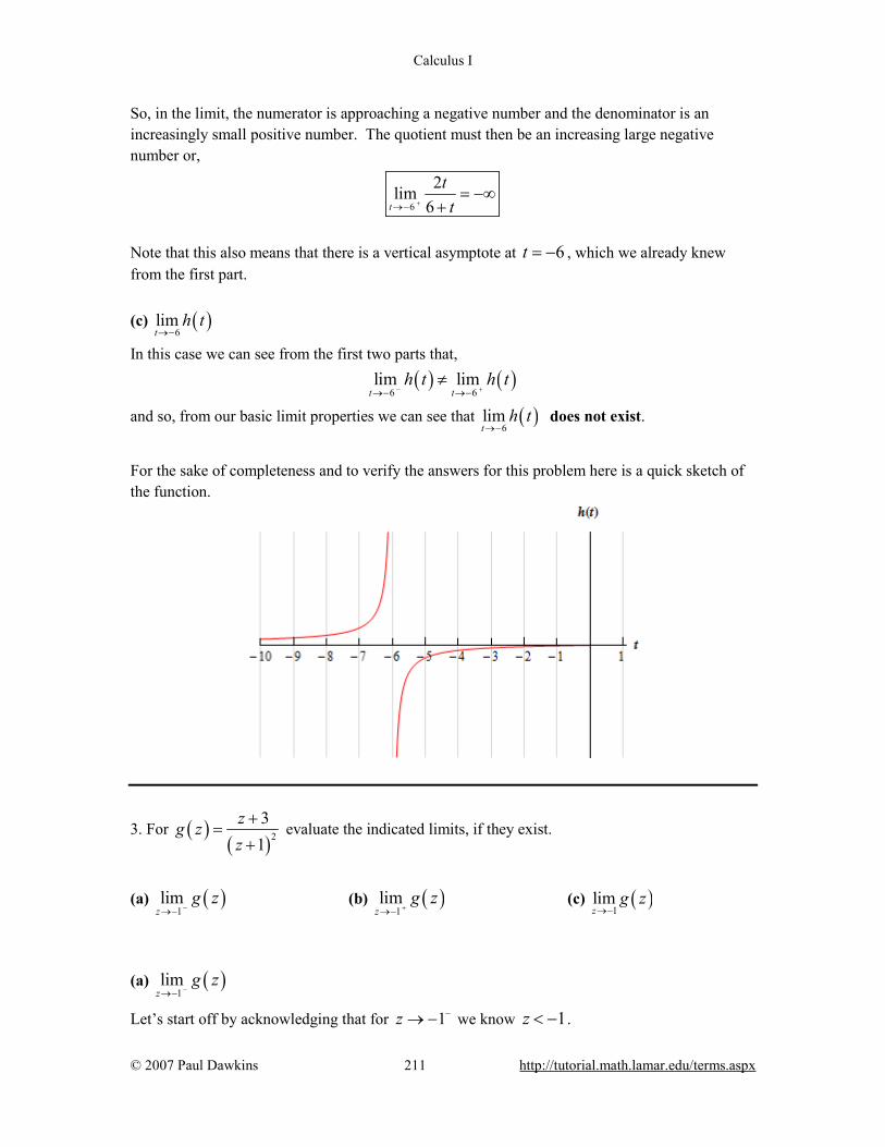
Calculus I
© 2007 Paul Dawkins 211 http://tutorial.math.lamar.edu/terms.aspx
So, in the limit, the numerator is approaching a negative number and the denominator is an increasingly small positive number. The quotient must then be an increasing large negative number or,
6
2lim6t
tt+→−
= −∞+
Note that this also means that there is a vertical asymptote at 6t = − , which we already knew from the first part. (c) ( )
6limt
h t→−
In this case we can see from the first two parts that, ( ) ( )
6 6lim lim
t th t h t
− +→− →−≠
and so, from our basic limit properties we can see that ( )6
limt
h t→−
does not exist.
For the sake of completeness and to verify the answers for this problem here is a quick sketch of the function.
3. For ( )( )2
31
zg zz
+=
+ evaluate the indicated limits, if they exist.
(a) ( )
1lim
zg z
−→− (b) ( )
1lim
zg z
+→− (c) ( )
1limz
g z→−
(a) ( )
1lim
zg z
−→−
Let’s start off by acknowledging that for 1z −→ − we know 1z < − .
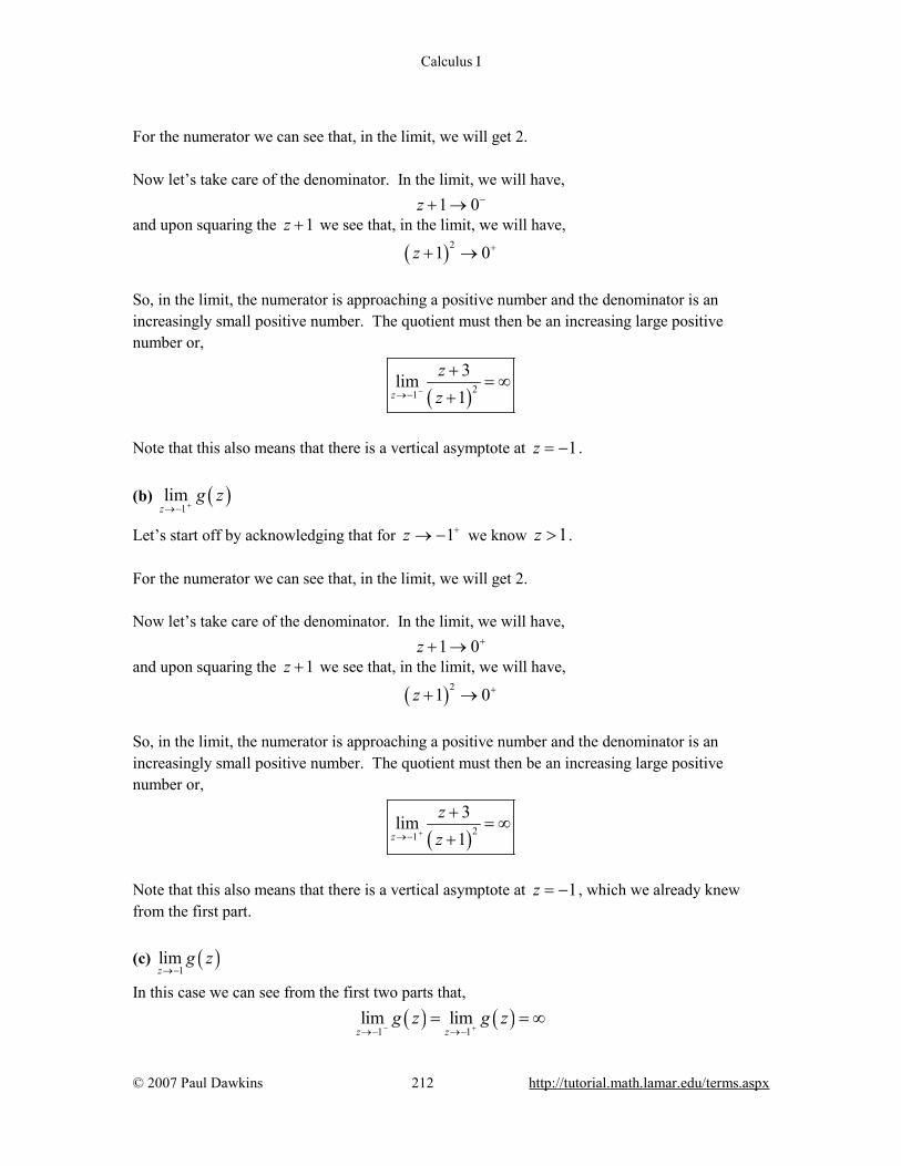
Calculus I
© 2007 Paul Dawkins 212 http://tutorial.math.lamar.edu/terms.aspx
For the numerator we can see that, in the limit, we will get 2. Now let’s take care of the denominator. In the limit, we will have, 1 0z −+ → and upon squaring the 1z + we see that, in the limit, we will have,
( )21 0z ++ → So, in the limit, the numerator is approaching a positive number and the denominator is an increasingly small positive number. The quotient must then be an increasing large positive number or,
( )21
3lim1z
zz−→−
+= ∞
+
Note that this also means that there is a vertical asymptote at 1z = − . (b) ( )
1lim
zg z
+→−
Let’s start off by acknowledging that for 1z +→ − we know 1z > . For the numerator we can see that, in the limit, we will get 2. Now let’s take care of the denominator. In the limit, we will have, 1 0z ++ → and upon squaring the 1z + we see that, in the limit, we will have,
( )21 0z ++ → So, in the limit, the numerator is approaching a positive number and the denominator is an increasingly small positive number. The quotient must then be an increasing large positive number or,
( )21
3lim1z
zz+→−
+= ∞
+
Note that this also means that there is a vertical asymptote at 1z = − , which we already knew from the first part. (c) ( )
1limz
g z→−
In this case we can see from the first two parts that, ( ) ( )
1 1lim lim
z zg z g z
− +→− →−= = ∞

Calculus I
© 2007 Paul Dawkins 213 http://tutorial.math.lamar.edu/terms.aspx
and so, from our basic limit properties we can see that,
( )1
limz
g z→−
= ∞
For the sake of completeness and to verify the answers for this problem here is a quick sketch of the function.
4. For ( ) 2
74
xg xx
+=
− evaluate the indicated limits, if they exist.
(a) ( )
2limx
g x−→
(b) ( )2
limx
g x+→
(c) ( )2
limx
g x→
(a) ( )
2limx
g x−→
Let’s start off by acknowledging that for 2x −→ we know 2x < . For the numerator we can see that, in the limit, we will get 9. Now let’s take care of the denominator. First, we know that if we square a number less than 2 (and greater than -2, which it is safe to assume we have here because we’re doing the limit) we will get a number that is less that 4 and so, in the limit, we will have, 2 4 0x −− → So, in the limit, the numerator is approaching a positive number and the denominator is an increasingly small negative number. The quotient must then be an increasing large negative number or,

Calculus I
© 2007 Paul Dawkins 214 http://tutorial.math.lamar.edu/terms.aspx
22
7lim4x
xx−→
+= −∞
−
Note that this also means that there is a vertical asymptote at 2x = . (b) ( )
2limx
g x+→
Let’s start off by acknowledging that for 2x +→ we know 2x > . For the numerator we can see that, in the limit, we will get 9. Now let’s take care of the denominator. First, we know that if we square a number greater than 2 we will get a number that is greater than 4 and so, in the limit, we will have, 2 4 0x +− → So, in the limit, the numerator is approaching a positive number and the denominator is an increasingly small positive number. The quotient must then be an increasing large positive number or,
22
7lim4x
xx+→
+= ∞
−
Note that this also means that there is a vertical asymptote at 2x = , which we already knew from the first part. (c) ( )
2limx
g x→
In this case we can see from the first two parts that, ( ) ( )
2 2lim limx x
g x g x− +→ →
≠
and so, from our basic limit properties we can see that ( )2
limx
g x→
does not exist.
For the sake of completeness and to verify the answers for this problem here is a quick sketch of the function.
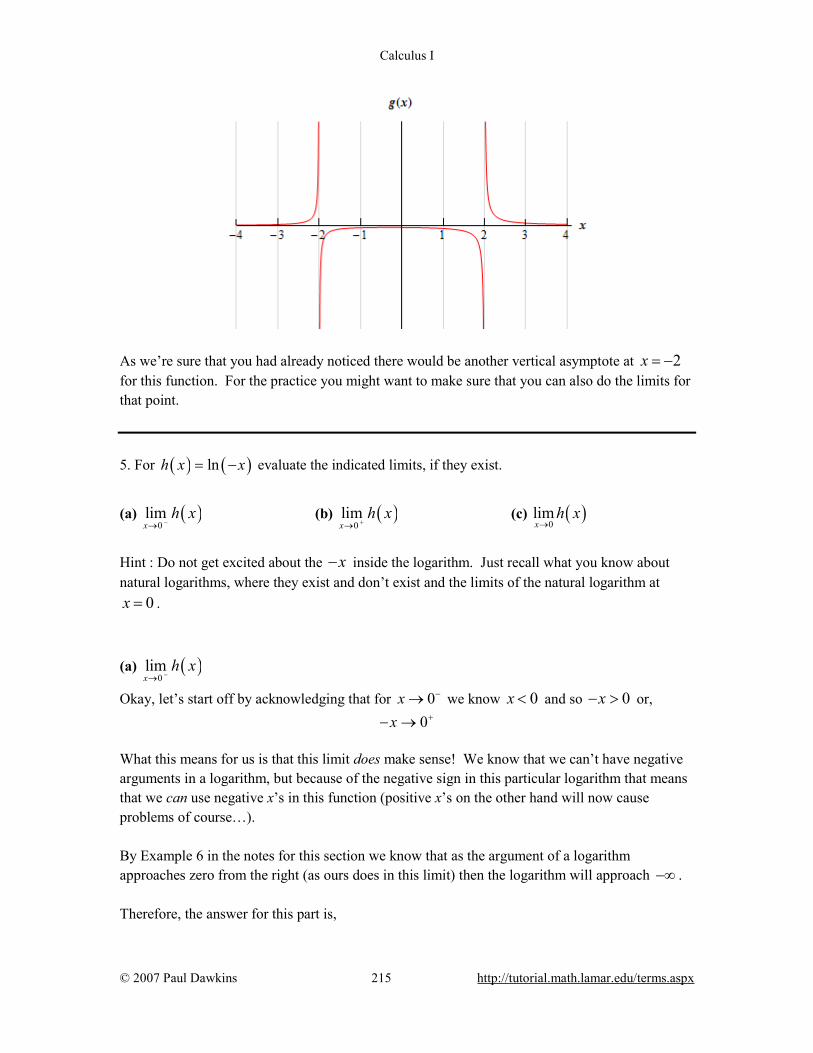
Calculus I
© 2007 Paul Dawkins 215 http://tutorial.math.lamar.edu/terms.aspx
As we’re sure that you had already noticed there would be another vertical asymptote at 2x = − for this function. For the practice you might want to make sure that you can also do the limits for that point. 5. For ( ) ( )lnh x x= − evaluate the indicated limits, if they exist.
(a) ( )
0limx
h x−→
(b) ( )0
limx
h x+→
(c) ( )0
limx
h x→
Hint : Do not get excited about the x− inside the logarithm. Just recall what you know about natural logarithms, where they exist and don’t exist and the limits of the natural logarithm at
0x = . (a) ( )
0limx
h x−→
Okay, let’s start off by acknowledging that for 0x −→ we know 0x < and so 0x− > or, 0x +− → What this means for us is that this limit does make sense! We know that we can’t have negative arguments in a logarithm, but because of the negative sign in this particular logarithm that means that we can use negative x’s in this function (positive x’s on the other hand will now cause problems of course…). By Example 6 in the notes for this section we know that as the argument of a logarithm approaches zero from the right (as ours does in this limit) then the logarithm will approach −∞ . Therefore, the answer for this part is,

Calculus I
© 2007 Paul Dawkins 216 http://tutorial.math.lamar.edu/terms.aspx
( )0
lim lnx
x−→
= −∞
(b) ( )
0limx
h x+→
In this part we know that for 0x +→ we have 0x > and so 0x− < . At this point we can stop. We know that we can’t have negative arguments in a logarithm and for this limit that is exactly what we’ll get and so ( )
0limx
h x+→
does not exist.
(c) ( )
0limx
h x→
The answer for this part is ( )0
limx
h x→
does not exist. We can use two lines of reasoning to justify
this. First, we are unable to look at both sides of the point in question and so there is no possible way for the limit to exist. The second line of reasoning is really the same as the first, but put in different terms. From the first two parts that, ( ) ( )
0 0lim limx x
h x h x− +→ →
≠
and so, from our basic limit properties we can see that ( )0
limx
h x→
does not exist.
For the sake of completeness and to verify the answers for this problem here is a quick sketch of the function.
6. For ( ) ( )tanR y y= evaluate the indicated limits, if they exist.

Calculus I
© 2007 Paul Dawkins 217 http://tutorial.math.lamar.edu/terms.aspx
(a) ( )32
limy
R yπ −
→ (b) ( )
32
limy
R yπ +
→ (c) ( )
32
limy
R yπ→
Hint : Don’t forget the graph of the tangent function. (a) ( )
32
limy
R yπ −
→
The easiest way to do this problem is from the graph of the tangent function so here is a quick sketch of the tangent function over several periods.
From the sketch we can see that,
( )32
lim tany
yπ −
→= ∞
(b) ( )
32
limy
R yπ +
→
From the graph in the first part we can see that,
( )32
lim tany
yπ +
→= −∞
(c) ( )
32
limy
R yπ→
From the first two parts that, ( ) ( )
3 32 2
lim limy y
R y R yπ π− +
→ →≠
and so, from our basic limit properties we can see that ( )32
limy
R yπ→
does not exist.
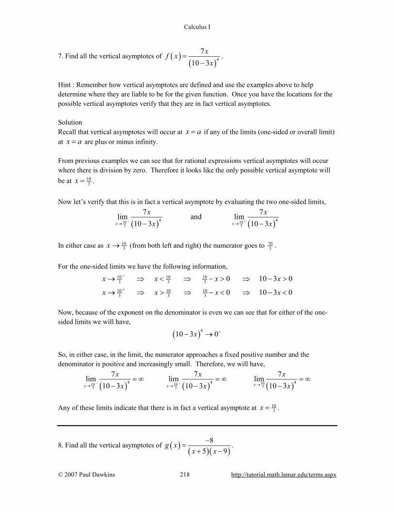
Calculus I
© 2007 Paul Dawkins 218 http://tutorial.math.lamar.edu/terms.aspx
7. Find all the vertical asymptotes of ( )( )4
710 3
xf xx
=−
.
Hint : Remember how vertical asymptotes are defined and use the examples above to help determine where they are liable to be for the given function. Once you have the locations for the possible vertical asymptotes verify that they are in fact vertical asymptotes. Solution Recall that vertical asymptotes will occur at x a= if any of the limits (one-sided or overall limit) at x a= are plus or minus infinity. From previous examples we can see that for rational expressions vertical asymptotes will occur where there is division by zero. Therefore it looks like the only possible vertical asymptote will be at 10
3x = . Now let’s verify that this is in fact a vertical asymptote by evaluating the two one-sided limits,
( ) ( )10 10
3 34 4
7 7lim and lim10 3 10 3x x
x xx x− +
→ →− −
In either case as 10
3x → (from both left and right) the numerator goes to 703 .
For the one-sided limits we have the following information,
10 10 103 3 3
10 10 103 3 3
0 10 3 0
0 10 3 0
x x x x
x x x x
−
+
→ ⇒ < ⇒ − > ⇒ − >
→ ⇒ > ⇒ − < ⇒ − <
Now, because of the exponent on the denominator is even we can see that for either of the one-sided limits we will have,
( )410 3 0x +− → So, in either case, in the limit, the numerator approaches a fixed positive number and the denominator is positive and increasingly small. Therefore, we will have,
( ) ( ) ( )1010 10 33 3
4 4 47 7 7lim lim lim
10 3 10 3 10 3xx x
x x xx x x− + →→ →
= ∞ = ∞ = ∞− − −
Any of these limits indicate that there is in fact a vertical asymptote at 10
3x = .
8. Find all the vertical asymptotes of ( ) ( )( )8
5 9g x
x x−
=+ −
.
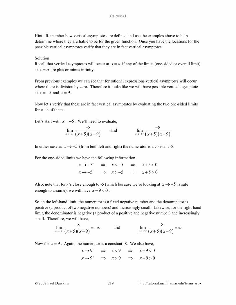
Calculus I
© 2007 Paul Dawkins 219 http://tutorial.math.lamar.edu/terms.aspx
Hint : Remember how vertical asymptotes are defined and use the examples above to help determine where they are liable to be for the given function. Once you have the locations for the possible vertical asymptotes verify that they are in fact vertical asymptotes. Solution Recall that vertical asymptotes will occur at x a= if any of the limits (one-sided or overall limit) at x a= are plus or minus infinity. From previous examples we can see that for rational expressions vertical asymptotes will occur where there is division by zero. Therefore it looks like we will have possible vertical asymptote at 5x = − and 9x = . Now let’s verify that these are in fact vertical asymptotes by evaluating the two one-sided limits for each of them. Let’s start with 5x = − . We’ll need to evaluate,
( )( ) ( ) ( )5 5
8 8lim and lim5 9 5 9x xx x x x− +→− →−
− −+ − + −
In either case as 5x → − (from both left and right) the numerator is a constant -8. For the one-sided limits we have the following information,
5 5 5 05 5 5 0
x x xx x x
−
+
→ − ⇒ < − ⇒ + <
→ − ⇒ > − ⇒ + > Also, note that for x’s close enough to -5 (which because we’re looking at 5x → − is safe enough to assume), we will have 9 0x − < . So, in the left-hand limit, the numerator is a fixed negative number and the denominator is positive (a product of two negative numbers) and increasingly small. Likewise, for the right-hand limit, the denominator is negative (a product of a positive and negative number) and increasingly small. Therefore, we will have,
( ) ( ) ( ) ( )5 5
8 8lim and lim5 9 5 9x xx x x x− +→− →−
− −= −∞ = ∞
+ − + −
Now for 9x = . Again, the numerator is a constant -8. We also have,
9 9 9 09 9 9 0
x x xx x x
−
+
→ ⇒ < ⇒ − <
→ ⇒ > ⇒ − >

Calculus I
© 2007 Paul Dawkins 220 http://tutorial.math.lamar.edu/terms.aspx
Finally, for x’s close enough to 9 (which because we’re looking at 9x → is safe enough to assume), we will have 5 0x + > . So, in the left-hand limit, the numerator is a fixed negative number and the denominator is negative (a product of a positive and negative number) and increasingly small. Likewise, for the right-hand limit, the denominator is negative (a product of two negative numbers) and increasingly small. Therefore, we will have,
( )( ) ( ) ( )9 9
8 8lim and lim5 9 5 9x xx x x x− +→ →
− −= ∞ = −∞
+ − + −
So, as all of these limits show we do in fact have vertical asymptotes at 5x = − and 9x = .
Limits At Infinity, Part I 1. For ( ) 7 34 18 9f x x x= − + evaluate each of the following limits.
(a) ( )limx
f x→−∞
(b) ( )limx
f x→∞
(a) ( )lim
xf x
→−∞
To do this all we need to do is factor out the largest power of x from the whole polynomial and then use basic limit properties along with Fact 1 from this section to evaluate the limit.
( )
( ) ( ) ( )
7 3 74 7
74 7
18 9lim 4 18 9 lim 4
18 9lim lim 4 4
x x
x x
x x xx x
xx x
→−∞ →−∞
→−∞ →−∞
− + = − + = − + = −∞ = −∞
(b) ( )lim
xf x
→∞
For this part all of the mathematical manipulations we did in the first part did not depend upon the limit itself and so don’t need to be redone here. We can pick up the problem right before we actually took the limits and then proceed.
( ) ( ) ( ) ( )7 3 74 7
18 9lim 4 18 9 lim lim 4 4x x x
x x xx x→∞ →∞ →∞
− + = − + = ∞ = ∞
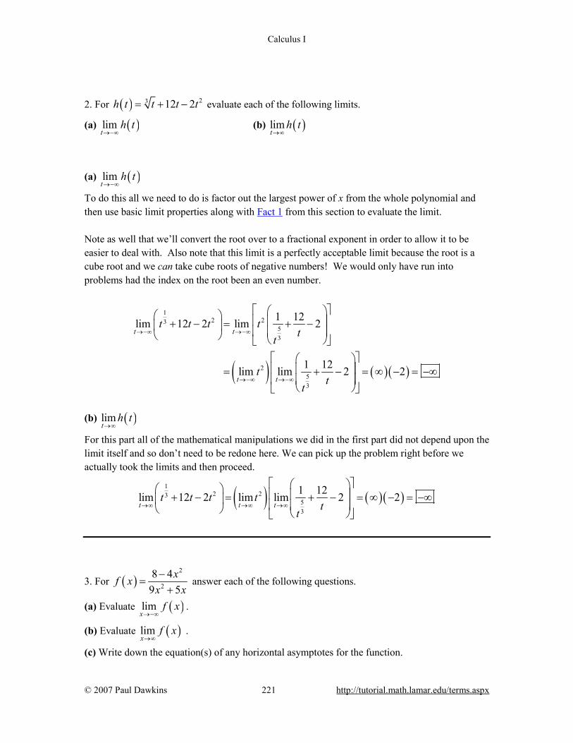
Calculus I
© 2007 Paul Dawkins 221 http://tutorial.math.lamar.edu/terms.aspx
2. For ( ) 23 12 2h t t t t= + − evaluate each of the following limits.
(a) ( )limt
h t→−∞
(b) ( )limt
h t→∞
(a) ( )lim
th t
→−∞
To do this all we need to do is factor out the largest power of x from the whole polynomial and then use basic limit properties along with Fact 1 from this section to evaluate the limit. Note as well that we’ll convert the root over to a fractional exponent in order to allow it to be easier to deal with. Also note that this limit is a perfectly acceptable limit because the root is a cube root and we can take cube roots of negative numbers! We would only have run into problems had the index on the root been an even number.
( ) ( )( )
12 23
53
253
1 12lim 12 2 lim 2
1 12lim lim 2 2
t t
t t
t t t ttt
ttt
→−∞ →−∞
→−∞ →−∞
+ − = + − = + − = ∞ − = −∞
(b) ( )lim
th t
→∞
For this part all of the mathematical manipulations we did in the first part did not depend upon the limit itself and so don’t need to be redone here. We can pick up the problem right before we actually took the limits and then proceed.
( ) ( )( )1
2 2353
1 12lim 12 2 lim lim 2 2t t t
t t t ttt
→∞ →∞ →∞
+ − = + − = ∞ − = −∞
3. For ( )2
2
8 49 5
xf xx x−
=+
answer each of the following questions.
(a) Evaluate ( )limx
f x→−∞
.
(b) Evaluate ( )limx
f x→∞
.
(c) Write down the equation(s) of any horizontal asymptotes for the function.
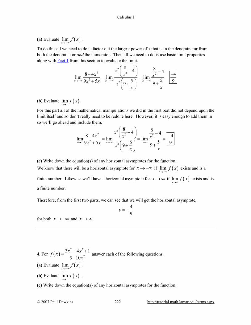
Calculus I
© 2007 Paul Dawkins 222 http://tutorial.math.lamar.edu/terms.aspx
(a) Evaluate ( )lim
xf x
→−∞.
To do this all we need to do is factor out the largest power of x that is in the denominator from both the denominator and the numerator. Then all we need to do is use basic limit properties along with Fact 1 from this section to evaluate the limit.
22 2 2
22
8 84 48 4 4lim lim lim 559 5 999x x x
xx x x
x x xxx
→−∞ →−∞ →−∞
− − − − = = =+ ++
(b) Evaluate ( )lim
xf x
→∞.
For this part all of the mathematical manipulations we did in the first part did not depend upon the limit itself and so don’t really need to be redone here. However, it is easy enough to add them in so we’ll go ahead and include them.
22 2 2
22
8 84 48 4 4lim lim lim 559 5 999x x x
xx x x
x x xxx
→∞ →∞ →∞
− − − − = = =+ ++
(c) Write down the equation(s) of any horizontal asymptotes for the function. We know that there will be a horizontal asymptote for x → −∞ if ( )lim
xf x
→−∞ exists and is a
finite number. Likewise we’ll have a horizontal asymptote for x → ∞ if ( )limx
f x→∞
exists and is
a finite number. Therefore, from the first two parts, we can see that we will get the horizontal asymptote,
49
y = −
for both x → −∞ and x → ∞ .
4. For ( )7 2
2
3 4 15 10
x xf xx
− +=
− answer each of the following questions.
(a) Evaluate ( )limx
f x→−∞
.
(b) Evaluate ( )limx
f x→∞
.
(c) Write down the equation(s) of any horizontal asymptotes for the function.
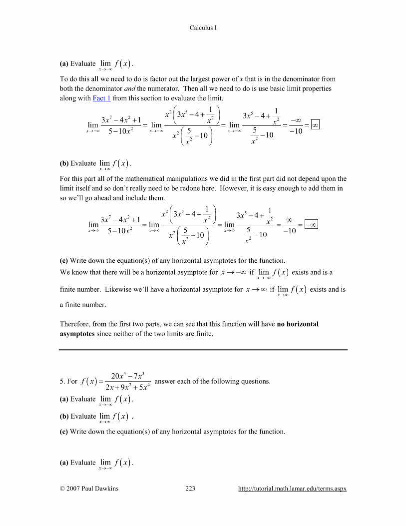
Calculus I
© 2007 Paul Dawkins 223 http://tutorial.math.lamar.edu/terms.aspx
(a) Evaluate ( )lim
xf x
→−∞.
To do this all we need to do is factor out the largest power of x that is in the denominator from both the denominator and the numerator. Then all we need to do is use basic limit properties along with Fact 1 from this section to evaluate the limit.
2 5 57 2 2 2
22
22
1 13 4 3 43 4 1lim lim lim 555 10 101010x x x
x x xx x x xx x
xx→−∞ →−∞ →−∞
− + − + − + −∞ = = = = ∞− − −−
(b) Evaluate ( )lim
xf x
→∞.
For this part all of the mathematical manipulations we did in the first part did not depend upon the limit itself and so don’t really need to be redone here. However, it is easy enough to add them in so we’ll go ahead and include them.
2 5 57 2 2 2
22
22
1 13 4 3 43 4 1lim lim lim 555 10 101010x x x
x x xx x x xx x
xx→∞ →∞ →∞
− + − + − + ∞ = = = = −∞− − −−
(c) Write down the equation(s) of any horizontal asymptotes for the function. We know that there will be a horizontal asymptote for x → −∞ if ( )lim
xf x
→−∞ exists and is a
finite number. Likewise we’ll have a horizontal asymptote for x → ∞ if ( )limx
f x→∞
exists and is
a finite number. Therefore, from the first two parts, we can see that this function will have no horizontal asymptotes since neither of the two limits are finite.
5. For ( )4 3
2 4
20 72 9 5
x xf xx x x
−=
+ + answer each of the following questions.
(a) Evaluate ( )limx
f x→−∞
.
(b) Evaluate ( )limx
f x→∞
.
(c) Write down the equation(s) of any horizontal asymptotes for the function. (a) Evaluate ( )lim
xf x
→−∞.
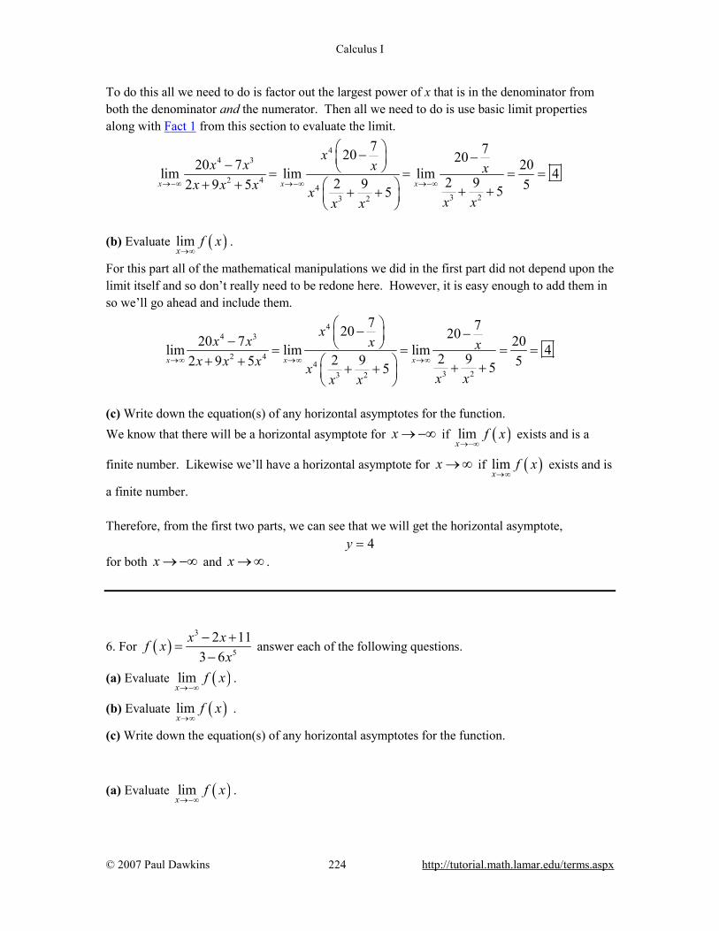
Calculus I
© 2007 Paul Dawkins 224 http://tutorial.math.lamar.edu/terms.aspx
To do this all we need to do is factor out the largest power of x that is in the denominator from both the denominator and the numerator. Then all we need to do is use basic limit properties along with Fact 1 from this section to evaluate the limit.
44 3
2 44
3 23 2
7 720 2020 7 20lim lim lim 42 92 92 9 5 555x x x
xx x x x
x x x xx xx x
→−∞ →−∞ →−∞
− − − = = = =+ + + ++ +
(b) Evaluate ( )lim
xf x
→∞.
For this part all of the mathematical manipulations we did in the first part did not depend upon the limit itself and so don’t really need to be redone here. However, it is easy enough to add them in so we’ll go ahead and include them.
44 3
2 44
3 23 2
7 720 2020 7 20lim lim lim 42 92 92 9 5 555x x x
xx x x x
x x x xx xx x
→∞ →∞ →∞
− − − = = = =+ + + ++ +
(c) Write down the equation(s) of any horizontal asymptotes for the function. We know that there will be a horizontal asymptote for x → −∞ if ( )lim
xf x
→−∞ exists and is a
finite number. Likewise we’ll have a horizontal asymptote for x → ∞ if ( )limx
f x→∞
exists and is
a finite number. Therefore, from the first two parts, we can see that we will get the horizontal asymptote, 4y = for both x → −∞ and x → ∞ .
6. For ( )3
5
2 113 6
x xf xx
− +=
− answer each of the following questions.
(a) Evaluate ( )limx
f x→−∞
.
(b) Evaluate ( )limx
f x→∞
.
(c) Write down the equation(s) of any horizontal asymptotes for the function. (a) Evaluate ( )lim
xf x
→−∞.
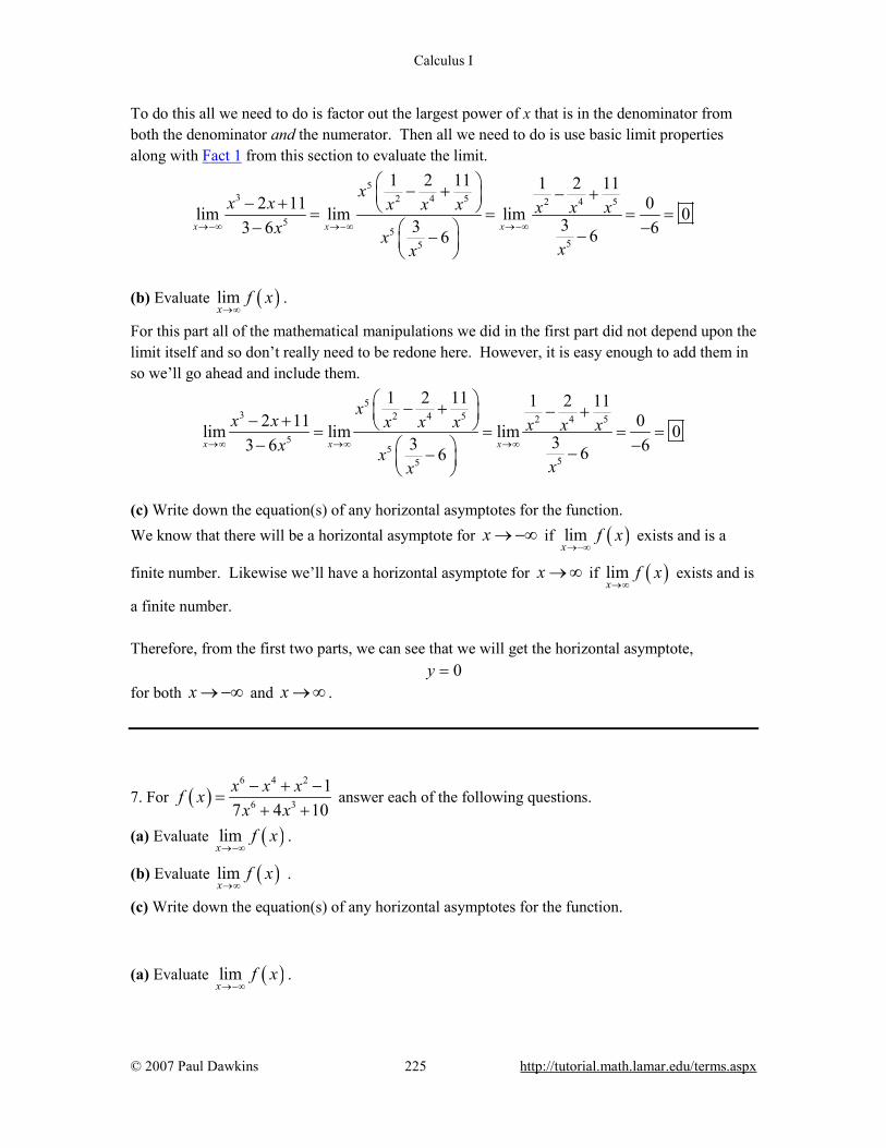
Calculus I
© 2007 Paul Dawkins 225 http://tutorial.math.lamar.edu/terms.aspx
To do this all we need to do is factor out the largest power of x that is in the denominator from both the denominator and the numerator. Then all we need to do is use basic limit properties along with Fact 1 from this section to evaluate the limit.
53 2 4 5 2 4 5
55
55
1 2 11 1 2 112 11 0lim lim lim 0333 6 666
x x x
xx x x x x x x x
x xxx
→−∞ →−∞ →−∞
− + − + − + = = = =− − −−
(b) Evaluate ( )lim
xf x
→∞.
For this part all of the mathematical manipulations we did in the first part did not depend upon the limit itself and so don’t really need to be redone here. However, it is easy enough to add them in so we’ll go ahead and include them.
53 2 4 5 2 4 5
55
55
1 2 11 1 2 112 11 0lim lim lim 0333 6 666
x x x
xx x x x x x x x
x xxx
→∞ →∞ →∞
− + − + − + = = = =− − −−
(c) Write down the equation(s) of any horizontal asymptotes for the function. We know that there will be a horizontal asymptote for x → −∞ if ( )lim
xf x
→−∞ exists and is a
finite number. Likewise we’ll have a horizontal asymptote for x → ∞ if ( )limx
f x→∞
exists and is
a finite number. Therefore, from the first two parts, we can see that we will get the horizontal asymptote, 0y = for both x → −∞ and x → ∞ .
7. For ( )6 4 2
6 3
17 4 10x x xf x
x x− + −
=+ +
answer each of the following questions.
(a) Evaluate ( )limx
f x→−∞
.
(b) Evaluate ( )limx
f x→∞
.
(c) Write down the equation(s) of any horizontal asymptotes for the function. (a) Evaluate ( )lim
xf x
→−∞.
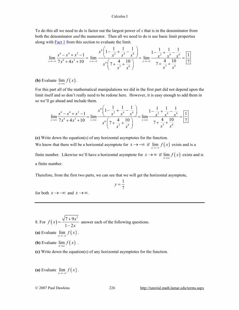
Calculus I
© 2007 Paul Dawkins 226 http://tutorial.math.lamar.edu/terms.aspx
To do this all we need to do is factor out the largest power of x that is in the denominator from both the denominator and the numerator. Then all we need to do is use basic limit properties along with Fact 1 from this section to evaluate the limit.
66 4 2 2 4 6 2 4 6
6 36
3 63 6
1 1 1 1 1 11 11 1lim lim lim 4 104 107 4 10 777x x x
xx x x x x x x x x
x x xx xx x
→−∞ →−∞ →−∞
− + − − + − − + − = = =+ + + ++ +
(b) Evaluate ( )lim
xf x
→∞.
For this part all of the mathematical manipulations we did in the first part did not depend upon the limit itself and so don’t really need to be redone here. However, it is easy enough to add them in so we’ll go ahead and include them.
66 4 2 2 4 6 2 4 6
6 36
3 63 6
1 1 1 1 1 11 11 1lim lim lim 4 104 107 4 10 777x x x
xx x x x x x x x x
x x xx xx x
→∞ →∞ →∞
− + − − + − − + − = = =+ + + ++ +
(c) Write down the equation(s) of any horizontal asymptotes for the function. We know that there will be a horizontal asymptote for x → −∞ if ( )lim
xf x
→−∞ exists and is a
finite number. Likewise we’ll have a horizontal asymptote for x → ∞ if ( )limx
f x→∞
exists and is
a finite number. Therefore, from the first two parts, we can see that we will get the horizontal asymptote,
17
y =
for both x → −∞ and x → ∞ .
8. For ( )27 9
1 2xf xx
+=
− answer each of the following questions.
(a) Evaluate ( )limx
f x→−∞
.
(b) Evaluate ( )limx
f x→∞
.
(c) Write down the equation(s) of any horizontal asymptotes for the function. (a) Evaluate ( )lim
xf x
→−∞.
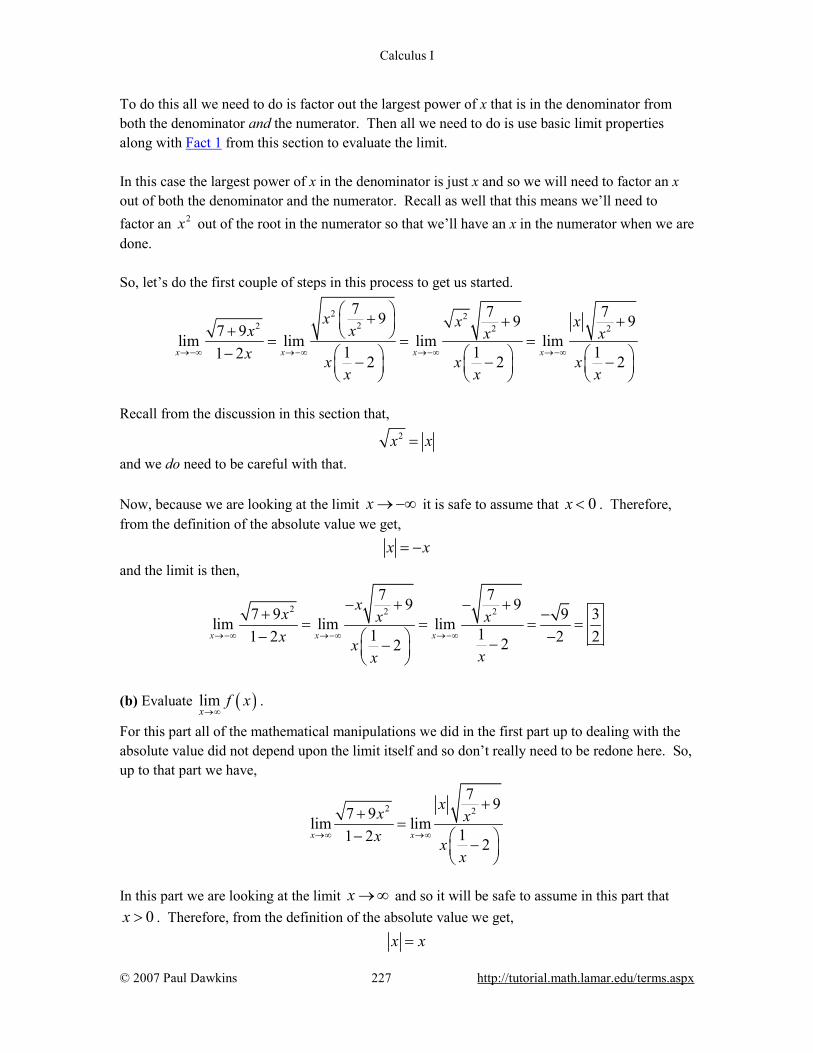
Calculus I
© 2007 Paul Dawkins 227 http://tutorial.math.lamar.edu/terms.aspx
To do this all we need to do is factor out the largest power of x that is in the denominator from both the denominator and the numerator. Then all we need to do is use basic limit properties along with Fact 1 from this section to evaluate the limit. In this case the largest power of x in the denominator is just x and so we will need to factor an x out of both the denominator and the numerator. Recall as well that this means we’ll need to factor an 2x out of the root in the numerator so that we’ll have an x in the numerator when we are done. So, let’s do the first couple of steps in this process to get us started.
2 222 2 2
7 7 79 9 97 9lim lim lim lim1 1 11 2 2 2 2
x x x x
x x xxx x xx x x x
x x x→−∞ →−∞ →−∞ →−∞
+ + + + = = =− − − −
Recall from the discussion in this section that,
2x x= and we do need to be careful with that. Now, because we are looking at the limit x → −∞ it is safe to assume that 0x < . Therefore, from the definition of the absolute value we get, x x= − and the limit is then,
2 2 2
7 79 97 9 9 3lim lim lim 111 2 2 222x x x
xx x xx x
xx→−∞ →−∞ →−∞
− + − ++ −= = = =
− − −−
(b) Evaluate ( )lim
xf x
→∞.
For this part all of the mathematical manipulations we did in the first part up to dealing with the absolute value did not depend upon the limit itself and so don’t really need to be redone here. So, up to that part we have,
2 2
7 97 9lim lim11 2 2
x x
xx xx x
x→∞ →∞
++=
− −
In this part we are looking at the limit x → ∞ and so it will be safe to assume in this part that
0x > . Therefore, from the definition of the absolute value we get,
x x=

Calculus I
© 2007 Paul Dawkins 228 http://tutorial.math.lamar.edu/terms.aspx
and the limit is then,
2 2 2
7 79 97 9 9 3lim lim lim 111 2 2 222x x x
xx x xx x
xx→∞ →∞ →∞
+ ++= = = = −
− − −−
(c) Write down the equation(s) of any horizontal asymptotes for the function. We know that there will be a horizontal asymptote for x → −∞ if ( )lim
xf x
→−∞ exists and is a
finite number. Likewise we’ll have a horizontal asymptote for x → ∞ if ( )limx
f x→∞
exists and is
a finite number. Therefore, from the first two parts, we can see that we will get the horizontal asymptote,
32
y =
for x → −∞ and we have the horizontal asymptote,
32
y = −
for x → ∞ .
9. For ( )2
82 3xf xx+
=+
answer each of the following questions.
(a) Evaluate ( )limx
f x→−∞
.
(b) Evaluate ( )limx
f x→∞
.
(c) Write down the equation(s) of any horizontal asymptotes for the function. (a) Evaluate ( )lim
xf x
→−∞.
To do this all we need to do is factor out the largest power of x that is in the denominator from both the denominator and the numerator. Then all we need to do is use basic limit properties along with Fact 1 from this section to evaluate the limit. For the denominator we need to be a little careful. The power of x in the denominator needs to be outside of the root so it can cancel against the x’s in the numerator. The largest power of x outside of the root that we can get (and leave something we can deal with in the root) will be just x. We get this by factoring an 2x out of the root. So, let’s do the first couple of steps in this process to get us started.

Calculus I
© 2007 Paul Dawkins 229 http://tutorial.math.lamar.edu/terms.aspx
2
222 22
8 8 81 1 18lim lim lim lim
3 332 3 2 22x x x x
x x xx x x xx x xx
x xx
→−∞ →−∞ →−∞ →−∞
+ + + + = = =+ + ++
Recall from the discussion in this section that,
2x x= and we do need to be careful with that. Now, because we are looking at the limit x → −∞ it is safe to assume that 0x < . Therefore, from the definition of the absolute value we get, x x= − and the limit is then,
2
2 2
8 81 18 1lim lim lim3 3 22 3 2 2
x x x
xx x xx x
x x→−∞ →−∞ →−∞
+ + + = = =−+ − + − +
(b) Evaluate ( )lim
xf x
→∞.
For this part all of the mathematical manipulations we did in the first part up to dealing with the absolute value did not depend upon the limit itself and so don’t really need to be redone here. So, up to that part we have,
2
2
818lim lim
32 3 2x x
xx xx x
x→∞ →∞
+ + =+ +
In this part we are looking at the limit x → ∞ and so it will be safe to assume in this part that
0x > . Therefore, from the definition of the absolute value we get,
x x= and the limit is then,
2
2 2
8 81 18 1lim lim lim3 3 22 3 2 2
x x x
xx x xx x
x x→∞ →∞ →∞
+ + + = = =+ + +
(c) Write down the equation(s) of any horizontal asymptotes for the function.

Calculus I
© 2007 Paul Dawkins 230 http://tutorial.math.lamar.edu/terms.aspx
We know that there will be a horizontal asymptote for x → −∞ if ( )limx
f x→−∞
exists and is a
finite number. Likewise we’ll have a horizontal asymptote for x → ∞ if ( )limx
f x→∞
exists and is
a finite number. Therefore, from the first two parts, we can see that we will get the horizontal asymptote,
12
y = −
for x → −∞ and we have the horizontal asymptote,
12
y =
for x → ∞ .
10. For ( )2
2 4
8 46 7
x xf xx x
+ −=
+ + answer each of the following questions.
(a) Evaluate ( )limx
f x→−∞
.
(b) Evaluate ( )limx
f x→∞
.
(c) Write down the equation(s) of any horizontal asymptotes for the function. (a) Evaluate ( )lim
xf x
→−∞.
To do this all we need to do is factor out the largest power of x that is in the denominator from both the denominator and the numerator. Then all we need to do is use basic limit properties along with Fact 1 from this section to evaluate the limit. For the denominator we need to be a little careful. The power of x in the denominator needs to be outside of the root so it can cancel against the x’s in the numerator. The largest power of x outside of the root that we can get (and leave something we can deal with in the root) will be just
2x . We get this by factoring an 4x out of the root. So, let’s do the first couple of steps in this process to get us started.

Calculus I
© 2007 Paul Dawkins 231 http://tutorial.math.lamar.edu/terms.aspx
22 2
2 44
4 2
2 22 2
4 24 2 4 2
8 1 48 4lim lim
6 16 7 7
8 1 8 14 4lim lim
6 1 6 17 7
x x
x x
xx x x xx x x
x x
x xx x x x
x xx x x x
→−∞ →−∞
→−∞ →−∞
+ − + − =+ + + +
+ − + − = =
+ + + +
Recall from the discussion in this section that,
2x x= So in this case we’ll have,
4 2 2x x x= =
and note that we can get rid of the absolute value bars because we know that 2 0x ≥ . So, let’s finish the limit up.
22 2 2
2 42
4 2 4 2
8 1 8 14 48 4 4lim lim lim6 1 6 1 76 7 7 7
x x x
xx x x x x xx x x
x x x x→−∞ →−∞ →−∞
+ − + − + − − = = =+ + + + + +
(b) Evaluate ( )lim
xf x
→∞.
Unlike the previous two problems with roots in them all of the mathematical manipulations in this case did not depend upon the actual limit because we were factoring an 2x out which will always be positive and so there will be no reason to redo all of that work. Here is this limit (with most of the work excluded), For this part all of the mathematical manipulations we did in the first part up to dealing with the absolute value did not depend upon the limit itself and so don’t really need to be redone here. So, up to that part we have,
22 2 2
2 42
4 2 4 2
8 1 8 14 48 4 4lim lim lim6 1 6 1 76 7 7 7
x x x
xx x x x x xx x x
x x x x→∞ →∞ →∞
+ − + − + − − = = =+ + + + + +
(c) Write down the equation(s) of any horizontal asymptotes for the function.
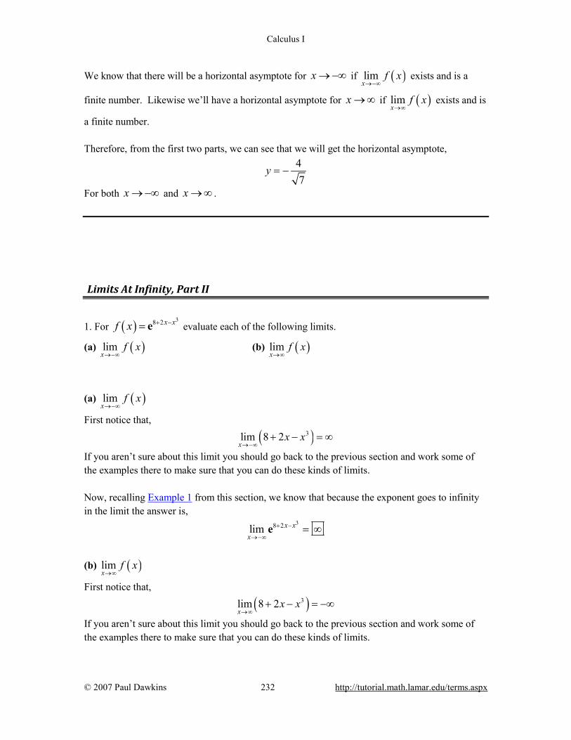
Calculus I
© 2007 Paul Dawkins 232 http://tutorial.math.lamar.edu/terms.aspx
We know that there will be a horizontal asymptote for x → −∞ if ( )limx
f x→−∞
exists and is a
finite number. Likewise we’ll have a horizontal asymptote for x → ∞ if ( )limx
f x→∞
exists and is
a finite number. Therefore, from the first two parts, we can see that we will get the horizontal asymptote,
47
y = −
For both x → −∞ and x → ∞ .
Limits At Infinity, Part II
1. For ( ) 38 2x xf x + −= e evaluate each of the following limits.
(a) ( )limx
f x→−∞
(b) ( )limx
f x→∞
(a) ( )lim
xf x
→−∞
First notice that,
( )3lim 8 2x
x x→−∞
+ − = ∞
If you aren’t sure about this limit you should go back to the previous section and work some of the examples there to make sure that you can do these kinds of limits. Now, recalling Example 1 from this section, we know that because the exponent goes to infinity in the limit the answer is,
38 2lim x x
x+ −
→−∞= ∞e
(b) ( )lim
xf x
→∞
First notice that,
( )3lim 8 2x
x x→∞
+ − = −∞
If you aren’t sure about this limit you should go back to the previous section and work some of the examples there to make sure that you can do these kinds of limits.
Calculus I
© 2007 Paul Dawkins 233 http://tutorial.math.lamar.edu/terms.aspx
Now, recalling Example 1 from this section, we know that because the exponent goes to negative infinity in the limit the answer is,
38 2lim 0x x
x+ −
→∞=e
2. For ( )26
5 3x x
xf x+
+= e evaluate each of the following limits.
(a) ( )limx
f x→−∞
(b) ( )limx
f x→∞
(a) ( )lim
xf x
→−∞
First notice that,
26lim
5 3x
x xx→−∞
+= −∞
+
If you aren’t sure about this limit you should go back to the previous section and work some of the examples there to make sure that you can do these kinds of limits. Now, recalling Example 1 from this section, we know that because the exponent goes to negative infinity in the limit the answer is,
26
5 3lim 0x x
xx
++
→−∞=e
(b) ( )lim
xf x
→∞
First notice that,
26lim
5 3x
x xx→∞
+= ∞
+
If you aren’t sure about this limit you should go back to the previous section and work some of the examples there to make sure that you can do these kinds of limits. Now, recalling Example 1 from this section, we know that because the exponent goes to infinity in the limit the answer is,
26
5 3limx x
xx
++
→∞= ∞e
3. For ( ) 6 7 42 10x x xf x −= − −e e e evaluate each of the following limits.
(a) ( )limx
f x→−∞
(b) ( )limx
f x→∞
Calculus I
© 2007 Paul Dawkins 234 http://tutorial.math.lamar.edu/terms.aspx
Hint : Remember that if there are two terms that seem to be suggesting that the function should be going in opposite directions that you’ll need to factor out of the function that term that is going to infinity faster to “prove” the limit. (a) ( )lim
xf x
→−∞
For this limit the exponentials with positive exponents will simply go to zero and there is only one exponential with a negative exponent (which will go to infinity) and so there isn’t much to do with this limit.
( )6 7 4lim 2 10 0 0x x xx
−
→−∞− − = − ∞ − = −∞e e e
(b) ( )lim
xf x
→∞
Here we have two exponents with positive exponents and so both will go to infinity in the limit. However each term has opposite signs and so each term seems to be suggesting different answers for the limit. In order to determine which “wins out” so to speak all we need to do is factor out the term with the largest exponent and then use basic limit properties.
( ) ( ) ( )( )6 7 4 6 13 2lim 2 10 lim 2 10 2x x x x x xx x
− − −
→∞ →∞ − − = − − = ∞ = ∞ e e e e e e
4. For ( ) 5 103 8x x xf x − −= − −e e e evaluate each of the following limits.
(a) ( )limx
f x→−∞
(b) ( )limx
f x→∞
Hint : Remember that if there are two terms that seem to be suggesting that the function should be going in opposite directions that you’ll need to factor out of the function that term that is going to infinity faster to “prove” the limit. (a) ( )lim
xf x
→−∞
Here we have two exponents with negative exponents and so both will go to infinity in the limit. However each term has opposite signs and so each term seems to be suggesting different answers for the limit. In order to determine which “wins out” so to speak all we need to do is factor out the term with the most negative exponent and then use basic limit properties.
( ) ( ) ( )( )5 10 5 4 15lim 3 8 lim 3 8 8x x x x x xx x
− − −
→−∞ →−∞ − − = − − = ∞ − = −∞ e e e e e e
Calculus I
© 2007 Paul Dawkins 235 http://tutorial.math.lamar.edu/terms.aspx
(b) ( )limx
f x→∞
For this limit the exponentials with negative exponents will simply go to zero and there is only one exponential with a positive exponent (which will go to infinity) and so there isn’t much to do with this limit.
( )5 10lim 3 8 0 0x x xx
− −
→∞− − = − − ∞ = −∞e e e
5. For ( )3 8
8 3
29 7
x x
x xf x−
−
−=
−e ee e
evaluate each of the following limits.
(a) ( )limx
f x→−∞
(b) ( )limx
f x→∞
Hint : Remember that you’ll need to factor the term in the denominator that is causing the denominator to go to infinity from both the numerator and denominator in order to evaluate this limit. (a) ( )lim
xf x
→−∞
The exponential with the negative exponent is the only term in the denominator going to infinity for this limit and so we’ll need to factor the exponential with the negative exponent in the denominator from both the numerator and denominator to evaluate this limit.
( )( )
3 113 8 11
8 3 113 11
1 22 1 2 1 0 1lim lim lim9 7 9 7 0 7 79 7
x xx x x
x x xx xx x x
−−
− −→−∞ →−∞ →−∞
−− − −= = = = −
− − −−
e ee e ee e ee e
(b) ( )lim
xf x
→∞
The exponential with the positive exponent is the only term in the denominator going to infinity for this limit and so we’ll need to factor the exponential with the positive exponent in the denominator from both the numerator and denominator to evaluate this limit.
( )( )
8 113 8 11
8 3 118 11
22 2 0 2 2lim lim lim9 7 9 7 9 0 99 7
x xx x x
x x xx xx x x
−− −
− −−→∞ →∞ →∞
−− − −= = = = −
− − −−
e ee e ee e ee e
6. For ( )7 3
10 4
216 2
x x x
x x xf x−
− −
− −=
+ +e e e
e e e evaluate each of the following limits.
(a) ( )limx
f x→−∞
(b) ( )limx
f x→∞

Calculus I
© 2007 Paul Dawkins 236 http://tutorial.math.lamar.edu/terms.aspx
Hint : Remember that you’ll need to factor the term in the denominator that is causing the denominator to go to infinity fastest from both the numerator and denominator in order to evaluate this limit. (a) ( )lim
xf x
→−∞
The exponentials with the negative exponents are the only terms in the denominator going to infinity for this limit and so we’ll need to factor the exponential with the most negative exponent in the denominator (because it will be going to infinity fastest) from both the numerator and denominator to evaluate this limit.
( )( )
4 3 77 3
10 4 4 3 14
3 7
3 14
5
5
22lim lim16 2 16 2
2 0 0lim16 2 0 0 2
x x x xx x x
x x x x x xx x
x x x
x xx
− −−
− − −→−∞ →−∞
−
→−∞
− −− −=
+ + + +
− − ∞ − −= = = ∞
+ + + +
e e e ee e ee e e e e e
e e ee e
(b) ( )lim
xf x
→∞
The exponentials with the positive exponents are the only terms in the denominator going to infinity for this limit and so we’ll need to factor the exponential with the most positive exponent in the denominator (because it will be going to infinity fastest) from both the numerator and denominator to evaluate this limit.
( )( )
10 17 7 97 3
10 4 10 11 14
17 7 9
11 14
22lim lim16 2 16 2
2 0 0 0lim 016 2 0 16 0
x x x xx x x
x x x x x xx x
x x x
x xx
− − −−
− − − −→−∞ →−∞
− − −
− −→−∞
− −− −=
+ + + +
− − − −= = =
+ + + +
e e e ee e ee e e e e e
e e ee e
7. Evaluate ( )3lim ln 4 9t
t t→−∞
− − .
Solution First notice that,
( )3lim 4 9t
t t→−∞
− − = ∞
If you aren’t sure about this limit you should go back to the previous section and work some of the examples there to make sure that you can do these kinds of limits. Now, recalling Example 5 from this section, we know that because the argument goes to infinity in the limit the answer is,
( )3lim ln 4 9t
t t→−∞
− − = ∞

Calculus I
© 2007 Paul Dawkins 237 http://tutorial.math.lamar.edu/terms.aspx
8. Evaluate 4
2
3 8lim ln2z
zz→−∞
− +
.
Solution First notice that,
4
2
3 8lim2z
zz→−∞
−= ∞
+
If you aren’t sure about this limit you should go back to the previous section and work some of the examples there to make sure that you can do these kinds of limits. Now, recalling Example 5 from this section, we know that because the argument goes to infinity in the limit the answer is,
4
2
3 8lim ln2z
zz→−∞
−= ∞ +
9. Evaluate 3
11 8lim ln7x
xx x→∞
+ +
.
Solution First notice that,
3
11 8lim 07x
xx x→∞
+=
+
If you aren’t sure about this limit you should go back to the previous section and work some of the examples there to make sure that you can do these kinds of limits. Also, note that because we are evaluating the limit x → ∞ it is safe to assume that 0x > and so we can further say that,
3
11 8 07
xx x
++→
+
Now, recalling Example 5 from this section, we know that because the argument goes to zero from the right in the limit the answer is,
3
11 8lim ln7x
xx x→∞
+ = −∞ +
10. Evaluate ( )1 5lim tan 7 3x
x x−
→−∞− + .

Calculus I
© 2007 Paul Dawkins 238 http://tutorial.math.lamar.edu/terms.aspx
Solution First notice that,
( )5lim 7 3x
x x→−∞
− + = −∞
If you aren’t sure about this limit you should go back to the previous section and work some of the examples there to make sure that you can do these kinds of limits. Now, recalling Example 7 from this section, we know that because the argument goes to negative infinity in the limit the answer is,
( )1 5lim tan 7 32x
x x π−
→−∞− + = −
11. Evaluate 1 4 7lim tan2t
tt
−
→∞
+ −
.
Solution First notice that,
4 7lim 72t
tt→∞
+= −
−
If you aren’t sure about this limit you should go back to the previous section and work some of the examples there to make sure that you can do these kinds of limits. Then answer is then,
( )1 14 7lim tan tan 72t
tt
− −
→∞
+ = − −
Do not get so used the “special case” limits that we tend to usually do in the problems at the end of a section that you decide that you must have done something wrong when you run across a problem that doesn’t fall in the “special case” category.
12. Evaluate 2 4
13
3 9lim tan4w
w ww w
−
→∞
− −
.
Solution First notice that,
2 4
3
3 9lim4w
w ww w→∞
−= ∞
−
If you aren’t sure about this limit you should go back to the previous section and work some of the examples there to make sure that you can do these kinds of limits.
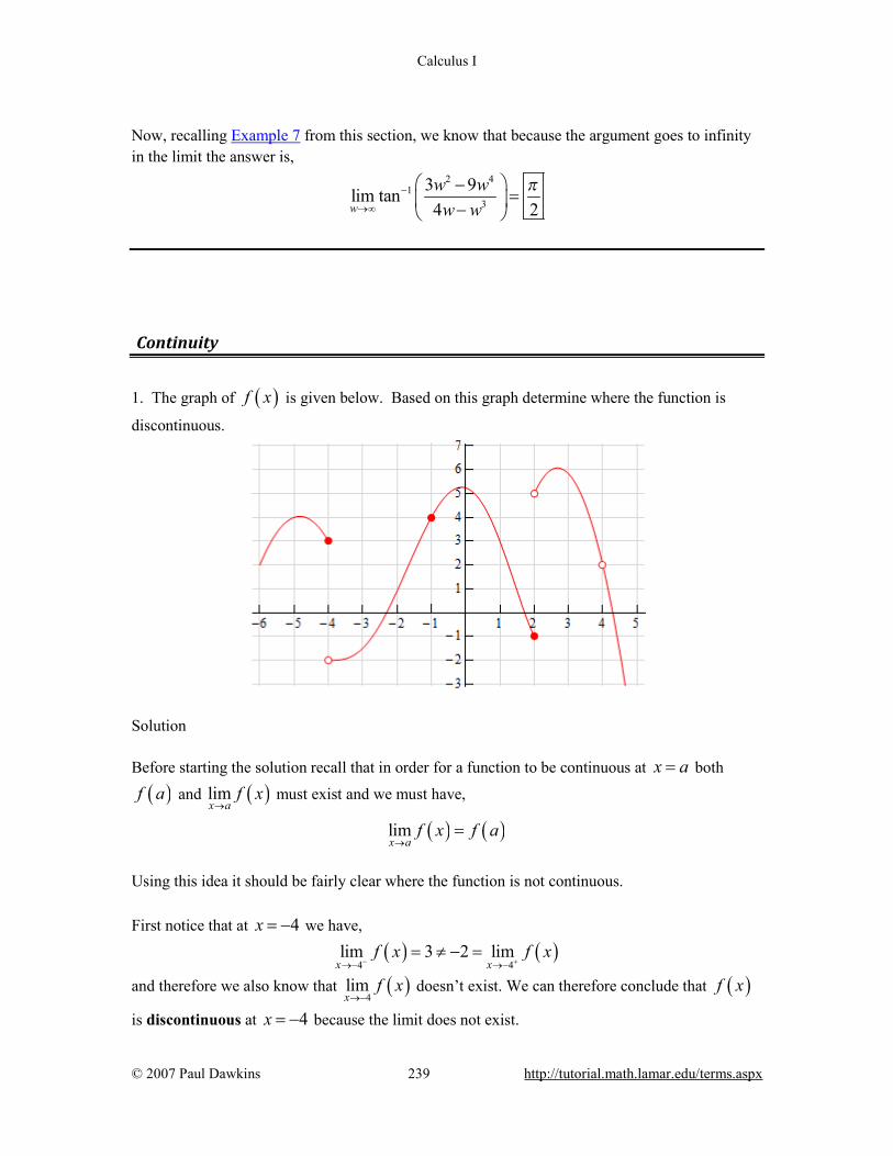
Calculus I
© 2007 Paul Dawkins 239 http://tutorial.math.lamar.edu/terms.aspx
Now, recalling Example 7 from this section, we know that because the argument goes to infinity in the limit the answer is,
2 4
13
3 9lim tan4 2w
w ww w
π−
→∞
−= −
Continuity 1. The graph of ( )f x is given below. Based on this graph determine where the function is
discontinuous.
Solution Before starting the solution recall that in order for a function to be continuous at x a= both
( )f a and ( )limx a
f x→
must exist and we must have,
( ) ( )limx a
f x f a→
=
Using this idea it should be fairly clear where the function is not continuous. First notice that at 4x = − we have,
( ) ( )4 4
lim 3 2 limx x
f x f x− +→− →−
= ≠ − =
and therefore we also know that ( )4
limx
f x→−
doesn’t exist. We can therefore conclude that ( )f x
is discontinuous at 4x = − because the limit does not exist.

Calculus I
© 2007 Paul Dawkins 240 http://tutorial.math.lamar.edu/terms.aspx
Likewise, at 2x = we have,
( ) ( )2 2
lim 1 5 limx x
f x f x− +→ →
= − ≠ =
and therefore we also know that ( )2
limx
f x→
doesn’t exist. So again, because the limit does not
exist, we can see that ( )f x is discontinuous at 2x = .
Finally let’s take a look at 4x = . Here we can see that,
( ) ( )4 4
lim 2 limx x
f x f x− +→ →
= =
and therefore we also know that ( )4
lim 2x
f x→
= . However, we can also see that ( )4f doesn’t
exist and so once again ( )f x is discontinuous at 4x = because this time the function does not
exist at 4x = . All other points on this graph will have both the function and limit exist and we’ll have
( ) ( )limx a
f x f a→
= and so will be continuous.
In summary then the points of discontinuity for this graph are : 4x = − , 2x = and 4x = . 2. The graph of ( )f x is given below. Based on this graph determine where the function is
discontinuous.
Solution Before starting the solution recall that in order for a function to be continuous at x a= both
( )f a and ( )limx a
f x→
must exist and we must have,
( ) ( )limx a
f x f a→
=

Calculus I
© 2007 Paul Dawkins 241 http://tutorial.math.lamar.edu/terms.aspx
Using this idea it should be fairly clear where the function is not continuous. First notice that at 8x = − we have,
( ) ( )8 8
lim 6 limx x
f x f x− +→− →−
= − =
and therefore we also know that ( )8
lim 6x
f x→−
= − . We can also see that ( )8 3f − = − and so we
have,
( ) ( )8
6 lim 8 3x
f x f→−
− = ≠ − = −
Because the function and limit have different values we can conclude that ( )f x is
discontinuous at 8x = − . Next let’s take a look at 2x = − we have,
( ) ( )2 2
lim 3 limx x
f x f x− +→− →−
= ≠ ∞ =
and therefore we also know that ( )2
limx
f x→−
doesn’t exist. We can therefore conclude that
( )f x is discontinuous at 2x = − because the limit does not exist.
Finally let’s take a look at 6x = . Here we can see we have,
( ) ( )6 6
lim 2 5 limx x
f x f x− +→ →
= ≠ =
and therefore we also know that ( )6
limx
f x→
doesn’t exist. So, once again, because the limit does
not exist, we can conclude that ( )f x is discontinuous at 6x = .
All other points on this graph will have both the function and limit exist and we’ll have
( ) ( )limx a
f x f a→
= and so will be continuous.
In summary then the points of discontinuity for this graph are : 8x = − , 2x = − and 6x = . 3. Using only Properties 1- 9 from the Limit Properties section, one-sided limit properties (if needed) and the definition of continuity determine if the following function is continuous or discontinuous at (a) 1x = − , (b) 0x = , (c) 3x = ?
( ) 4 59 3
xf xx
+=
−
(a) 1x = − Before starting off with the solution to this part notice that we CAN NOT do what we’ve commonly done to evaluate limits to this point. In other words, we can’t just plug in the point to
Calculus I
© 2007 Paul Dawkins 242 http://tutorial.math.lamar.edu/terms.aspx
evaluate the limit. Doing this implicitly assumes that the function is continuous at the point and that is what we are being asked to determine here. Therefore the only way for us to compute the limit is to go back to the properties from the Limit Properties section and compute the limit as we did back in that section. We won’t be putting all the details here so if you need a little refresher on doing this you should go back to the problems from that section and work a few of them. So, here we go.
( )( )( )
( )( ) ( )1 1 1
1 11 1 1
lim 4 5 4 lim lim 5 4 1 54 5lim lim 19 3 lim 9 3 lim 9 3 lim 9 3 1
x x xx x
x x x
x xxf x fx x x
→− →− →−
→− →−→− →− →−
+ + − ++= = = = = −
− − − − −
So, we can see that ( ) ( )
1lim 1x
f x f→−
= − and so the function is continuous at 1x = − .
(b) 0x = For justification on why we can’t just plug in the number here check out the comment at the beginning of the solution to (a). Here is the work for this part.
( )( )( )
( )( ) ( )0 0 0
0 00 0 0
lim 4 5 4lim lim5 4 0 54 5lim lim 09 3 lim 9 3 lim9 3lim 9 3 0
x x xx x
x x x
x xxf x fx x x
→ → →
→ →→ → →
+ + ++= = = = =
− − − −
So, we can see that ( ) ( )
0lim 0x
f x f→
= and so the function is continuous at 0x = .
(c) 3x = For justification on why we can’t just plug in the number here check out the comment at the beginning of the solution to (a). Although there is also of course the problem here that ( )3f
doesn’t exist and so we couldn’t plug in the value even if we wanted to. This also tells us what we need to know however. As noted in the notes for this section if either the function or the limit do not exist then the function is not continuous at the point. Therefore we can see that the function is not continuous at 3x = . For practice you might want to verify that,
( ) ( )3 3
lim limx x
f x f x− +→ →
= ∞ = −∞
and so ( )3
limx
f x→
also doesn’t exist.
Calculus I
© 2007 Paul Dawkins 243 http://tutorial.math.lamar.edu/terms.aspx
4. Using only Properties 1- 9 from the Limit Properties section, one-sided limit properties (if needed) and the definition of continuity determine if the following function is continuous or discontinuous at (a) 2z = − , (b) 0z = , (c) 5z = ?
( ) 2
63 10
g zz z
=− −
(a) 2z = − Before starting off with the solution to this part notice that we CAN NOT do what we’ve commonly done to evaluate limits to this point. In other words, we can’t just plug in the point to evaluate the limit. Doing this implicitly assumes that the function is continuous at the point and that is what we are being asked to determine here. Of course even if we had tried to plug in the point we would have run into problems as ( )2g −
doesn’t exist and this tell us all we need to know. As noted in the notes for this section if either the function or the limit do not exist then the function is not continuous at the point. Therefore we can see that the function is not continuous at 2z = − . For practice you might want to verify that,
( ) ( )2 2
lim limz z
g z g z− +→− →−
= ∞ = −∞
and so ( )2
limz
g z→−
also doesn’t exist.
(b) 0z = For justification on why we can’t just plug in the number here check out the comment at the beginning of the solution to (a). Therefore, because we can’t just plug the point into the function, the only way for us to compute the limit is to go back to the properties from the Limit Properties section and compute the limit as we did back in that section. We won’t be putting all the details here so if you need a little refresher on doing this you should go back to the problems from that section and work a few of them. Here is the work for this part.
( ) ( )
( ) ( )
0 02 220 0
0 0 00
2
lim 6 lim 66lim lim3 10 lim 3lim lim10lim 3 10
6 00 3 0 10
z zz z
z z zz
g zz z z zz z
g
→ →
→ →→ → →→
= = =− − − −− −
= =− −
So, we can see that ( ) ( )
0lim 0z
g x g→
= and so the function is continuous at 0z = .

Calculus I
© 2007 Paul Dawkins 244 http://tutorial.math.lamar.edu/terms.aspx
(c) 5z = For justification on why we can’t just plug in the number here check out the comment at the beginning of the solution to (a). Although there is also of course the problem here that ( )5g
doesn’t exist and so we couldn’t plug in the value even if we wanted to. This also tells us what we need to know however. As noted in the notes for this section if either the function of the limit do not exist then the function is not continuous at the point. Therefore we can see that the function is not continuous at 5z = . For practice you might want to verify that,
( ) ( )5 5
lim limz z
g z g z− +→ →
= −∞ = ∞
and so ( )5
limz
g z→
also doesn’t exist.
5. Using only Properties 1- 9 from the Limit Properties section, one-sided limit properties (if needed) and the definition of continuity determine if the following function is continuous or discontinuous at (a) 4x = , (b) 6x = ?
( ) 2 61 6
x xg x
x x<
= − ≥
(a) 4x = Before starting off with the solution to this part notice that we CAN NOT do what we’ve commonly done to evaluate limits to this point. In other words, we can’t just plug in the point to evaluate the limit. Doing this implicitly assumes that the function is continuous at the point and that is what we are being asked to determine here. Therefore the only way for us to compute the limit is to go back to the properties from the Limit Properties section and compute the limit as we did back in that section. We won’t be putting all the details here so if you need a little refresher on doing this you should go back to the problems from that section and work a few of them. For this part we can notice that because there are values of x on both sides of 4x = in the range
6x < we won’t need to worry about one-sided limits here. Here is the work for this part.
( ) ( ) ( ) ( )4 4 4
lim lim 2 2lim 2 4 4x x x
g x x x g→ → →
= = = =
So, we can see that ( ) ( )
4lim 4x
g x g→
= and so the function is continuous at 4x = .
(b) 6x =

Calculus I
© 2007 Paul Dawkins 245 http://tutorial.math.lamar.edu/terms.aspx
For justification on why we can’t just plug in the number here check out the comment at the beginning of the solution to (a). For this part we have the added complication that the point we’re interested in is also the “cut-off” point of the piecewise function and so we’ll need to take a look at the two one sided limits to compute the overall limit and again because we are being asked to determine if the function is continuous at this point we’ll need to resort to basic limit properties to compute the one-sided limits and not just plug in the point (which assumes continuity again…). Here is the work for this part.
( ) ( ) ( )
( ) ( )6 6 6
6 6 6 6
lim lim 2 2 lim 2 4 8
lim lim 1 lim lim 1 4 1 3x x x
x x x x
g x x x
g x x x− − −
+ + + +
→ → →
→ → → →
= = = =
= − = − = − =
So we can see that, ( ) ( )
6 6lim limx x
g x g x− +→ →
≠ and so ( )6
limx
g x→
does not exist.
Now, as discussed in the notes for this section, in order for a function to be continuous at a point both the function and the limit must exist. Therefore this function is not continuous at 6x =because ( )
6limx
g x→
does not exist.
6. Using only Properties 1- 9 from the Limit Properties section, one-sided limit properties (if needed) and the definition of continuity determine if the following function is continuous or discontinuous at (a) 2t = − , (b) 10t = ?
( )2 26 2
t th t
t t < −
= + ≥ −
(a) 2t = − Before starting off with the solution to this part notice that we CAN NOT do what we’ve commonly done to evaluate limits to this point. In other words, we can’t just plug in the point to evaluate the limit. Doing this implicitly assumes that the function is continuous at the point and that is what we are being asked to determine here. Therefore the only way for us to compute the limit is to go back to the properties from the Limit Properties section and compute the limit as we did back in that section. We won’t be putting all the details here so if you need a little refresher on doing this you should go back to the problems from that section and work a few of them. Also notice that for this part we have the added complication that the point we’re interested in is also the “cut-off” point of the piecewise function and so we’ll need to take a look at the two one

Calculus I
© 2007 Paul Dawkins 246 http://tutorial.math.lamar.edu/terms.aspx
sided limits to compute the overall limit and again because we are being asked to determine if the function is continuous at this point we’ll need to resort to basic limit properties to compute the one-sided limits and not just plug in the point (which assumes continuity again…). Here is the work for this part.
( ) ( )
( ) ( )
22
2 2
2 2 2 2
lim lim 2 4
lim lim 6 lim lim 6 2 6 4t t
t t t t
h t t
g t t t
− −
+ + + +
→− →−
→− →− →− →−
= = − =
= + = + = − + =
So we can see that, ( ) ( )
2 2lim lim 4
t th t h t
− +→− →−= = and so ( )
2lim 4t
h t→−
= .
Next, a quick computation shows us that ( )2 2 6 4h − = − + = and so we can see that
( ) ( )2
lim 2t
h t h→−
= − and so the function is continuous at 2t = − .
(b) 10t = For justification on why we can’t just plug in the number here check out the comment at the beginning of the solution to (a). For this part we can notice that because there are values of t on both sides of 10t = in the range
2t ≥ − we won’t need to worry about one-sided limits here. Here is the work for this part. Here is the work for this part. ( ) ( ) ( )
10 10 10 10lim lim 6 lim lim 6 10 6 10t t t t
h t t t h→ → → →
= + = + = + =
So, we can see that ( ) ( )
10lim 10t
h t h→
= and so the function is continuous at 10t = .
7. Using only Properties 1- 9 from the Limit Properties section, one-sided limit properties (if needed) and the definition of continuity determine if the following function is continuous or discontinuous at (a) 6x = − , (b) 1x = ?
( ) 3
1 3 67 6
6 11 1
2 1
x xx
g x x xx
x x
− < − = −= − < < =
− >
(a) 6x = −
Calculus I
© 2007 Paul Dawkins 247 http://tutorial.math.lamar.edu/terms.aspx
Before starting off with the solution to this part notice that we CAN NOT do what we’ve commonly done to evaluate limits to this point. In other words, we can’t just plug in the point to evaluate the limit. Doing this implicitly assumes that the function is continuous at the point and that is what we are being asked to determine here. Therefore the only way for us to compute the limit is to go back to the properties from the Limit Properties section and compute the limit as we did back in that section. We won’t be putting all the details here so if you need a little refresher on doing this you should go back to the problems from that section and work a few of them. Also notice that for this part we have the added complication that the point we’re interested in is also the “cut-off” point of the piecewise function and so we’ll need to take a look at the two one sided limits to compute the overall limit and again because we are being asked to determine if the function is continuous at this point we’ll need to resort to basic limit properties to compute the one-sided limits and not just plug in the point (which assumes continuity again…). Here is the work for this part.
( ) ( ) ( )
( ) ( )6 6 6 6
33
6 6
lim lim 1 3 lim 1 3 lim 1 3 6 19
lim lim 6 216
x x x x
x x
g x x x
g x x
− − − −
+ +
→− →− →− →−
→− →−
= − = − = − − =
= = − = −
So we can see that, ( ) ( )
6 6lim lim
x xg x g x
− +→− →−≠ and so ( )
6limx
g x→−
does not exist.
Now, as discussed in the notes for this section, in order for a function to be continuous at a point both the function and the limit must exist. Therefore this function is not continuous at 6x = −because ( )
6limx
g x→−
does not exist.
(b) 1x = For justification on why we can’t just plug in the number here check out the comment at the beginning of the solution to (a). Again note that we are dealing with another “cut-off” point here so we’ll need to use one-sided limits again as we did in the previous part. Here is the work for this part.
( )
( ) ( )
3 3
1 1
1 1 1 1
lim lim 1 1
lim lim 2 lim 2 lim 2 1 1x x
x x x x
g x x
g x x x− −
+ + + +
→ →
→ → → →
= = =
= − = − = − =
So we can see that, ( ) ( )
1 1lim lim 1x x
g x g x− +→ →
= = and so ( )1
lim 1x
g x→
= .
Calculus I
© 2007 Paul Dawkins 248 http://tutorial.math.lamar.edu/terms.aspx
Next, a quick computation shows us that ( )1 1g = and so we can see that ( ) ( )
1lim 1x
g x g→
= and
so the function is continuous at 1x = . 8. Determine where the following function is discontinuous.
( )2
2
93 2 8
xf xx x
−=
+ −
Hint : If we have two continuous functions and form a rational expression out of them recall where the rational expression will be discontinuous. We discussed this in the Limit Properties section, although we were using the phrase “nice enough” there instead of the word “continuity”. Solution As noted in the hint for this problem when dealing with a rational expression in which both the numerator and denominator are continuous (as we have here since both are polynomials) the only points in which the rational expression will be discontinuous will be where we have division by zero. Therefore, all we need to do is determine where the denominator is zero and that is fairly easy for this problem.
( )( )2 43 2 8 3 4 2 0 , 23
x x x x x x+ − = − + = ⇒ = = −
The function will therefore be discontinuous at the points : 43
x = and 2x = − .
9. Determine where the following function is discontinuous.
( ) 2
89 1tR t
t t=
− −
Hint : If we have two continuous functions and form a rational expression out of them recall where the rational expression will be discontinuous. We discussed this in the Limit Properties section, although we were using the phrase “nice enough” there instead of the word “continuity”. Solution As noted in the hint for this problem when dealing with a rational expression in which both the numerator and denominator are continuous (as we have here since both are polynomials) the only

Calculus I
© 2007 Paul Dawkins 249 http://tutorial.math.lamar.edu/terms.aspx
points in which the rational expression will be discontinuous will be where we have division by zero. Therefore, all we need to do is determine where the denominator is zero and that is fairly easy for this problem.
( ) ( ) ( )
( )
2
2 9 9 4 1 1 9 859 1 0 0.10977, 9.109772 1 2
t t t± − − − ±
− − = ⇒ = = = −
The function will therefore be discontinuous at the points : 9 85
2t ±
= .
10. Determine where the following function is discontinuous.
( ) ( )1
2 4cos 3h z
z=
−
Hint : If we have two continuous functions and form a rational expression out of them recall where the rational expression will be discontinuous. We discussed this in the Limit Properties section, although we were using the phrase “nice enough” there instead of the word “continuity”. Solution As noted in the hint for this problem when dealing with a rational expression in which both the numerator and denominator are continuous (as we have here since the numerator is just a constant and the denominator is a sum of continuous functions) the only points in which the rational expression will be discontinuous will be where we have division by zero. Therefore, all we need to do is determine where the denominator is zero. If you don’t recall how to solve equations involving trig functions you should go back to the Review chapter and take a look at the Solving Trig Equations sections there. Here is the solution work for determining where the denominator is zero. Using our calculator we get,
( ) 1 12 4cos 3 0 3 cos 1.04722
z x − − = → = =
The second angle will be in the fourth quadrant and is 2 1.0472 5.2360π − = . The denominator will therefore be zero at,

Calculus I
© 2007 Paul Dawkins 250 http://tutorial.math.lamar.edu/terms.aspx
3 1.0472 2 OR 3 5.2360 2 0, 1, 2,
2 20.3491 OR 1.7453 0, 1, 2,3 3
x n x n nn nx x n
π ππ π
= + = + = ± ±
= + = + = ± ±
…
…
The function will therefore be discontinuous at the points,
2 20.3491 OR 1.7453 0, 1, 2,3 3
n nx x nπ π= + = + = ± ± …
Note as well that this was one of the few trig equations that could be solved exactly if you know you basic unit circle values. Here is the exact solution for the points of discontinuity.
2 5 2OR 0, 1, 2,9 3 9 3
n nx x nπ π π π= + = + = ± ± …
11. Determine where the following function is discontinuous.
( ) 2 37 xxy x +=
− e
Hint : If we have two continuous functions and form a rational expression out of them recall where the rational expression will be discontinuous. We discussed this in the Limit Properties section, although we were using the phrase “nice enough” there instead of the word “continuity”. Solution As noted in the hint for this problem when dealing with a rational expression in which both the numerator and denominator are continuous (as we have here since the numerator is a polynomial and the denominator is a sum of two continuous functions) the only points in which the rational expression will be discontinuous will be where we have division by zero. Therefore, all we need to do is determine where the denominator is zero and that is fairly easy for this problem.
( ) ( )( )2 3 2 3 17 0 7 2 3 ln 7 ln 7 3 0.52702
x x x x+ +− = → = → + = ⇒ = − = −e e
The function will therefore be discontinuous at : ( )( )1 ln 7 3 0.52702
x = − = − .
12. Determine where the following function is discontinuous. ( ) ( )tan 2g x x=

Calculus I
© 2007 Paul Dawkins 251 http://tutorial.math.lamar.edu/terms.aspx
Hint : If we have two continuous functions and form a rational expression out of them recall where the rational expression will be discontinuous. We discussed this in the Limit Properties section, although we were using the phrase “nice enough” there instead of the word “continuity”. And, yes we really do have a rational expression here… Solution As noted in the hint for this problem when dealing with a rational expression in which both the numerator and denominator are continuous the only points in which the rational expression will not be continuous will be where we have division by zero. Also, writing the function as,
( ) ( )( )
sin 2cos 2
xg x
x=
we can see that we really do have a rational expression here. Therefore, all we need to do is determine where the denominator (i.e. cosine) is zero. If you don’t recall how to solve equations involving trig functions you should go back to the Review chapter and take a look at the Solving Trig Equations sections there. Here is the solution work for determining where the denominator is zero. Using our basic unit circle knowledge we know where cosine will be zero so we have,
32 2 OR 2 2 0, 1, 2,2 2
x n x n nπ ππ π= + = + = ± ± …
The denominator will therefore be zero, and the function will be discontinuous, at,
3OR 0, 1, 2,4 4
x n x n nπ ππ π= + = + = ± ± …
13. Use the Intermediate Value Theorem to show that 2 325 8 0x x− − = has at least one root in the interval [ ]2,4− . Note that you are NOT asked to find the solution only show that at least one
must exist in the indicated interval, Hint : The hardest part of these problems for most students is just getting started. First, you need to determine the value of “M” that you need to use and then actually use the Intermediate Value Theorem. So, go back to the IVT and compare the conclusions of the theorem and it should be pretty obvious what the M should be and then just check that the hypothesis (i.e. the “requirements” of the theorem) are met and you’ll pretty much be done. Solution Okay, let’s start off by defining,
Calculus I
© 2007 Paul Dawkins 252 http://tutorial.math.lamar.edu/terms.aspx
( ) 2 325 8 & 0f x x x M= − − = The problem is then asking us to show that there is a c in [ ]2,4− so that,
( ) 0f c M= = but this is exactly the second conclusion of the Intermediate Value Theorem. So, let’s see that the “requirements” of the theorem are met. First, the function is a polynomial and so is continuous everywhere and in particular is continuous on the interval [ ]2,4− . Note that this IS a requirement that MUST be met in order to use the IVT
and it is the one requirement that is most often overlooked. If we don’t have a continuous function the IVT simply can’t be used. Now all that we need to do is verify that M is between the function values as the endpoints of the interval. So, ( ) ( )2 1 4 167f f− = = − Therefore we have, ( ) ( )4 167 0 1 2f f= − < < = − So by the Intermediate Value Theorem there must be a number c such that, ( )2 4 & 0c f c− < < = and we have shown what we were asked to show. 14. Use the Intermediate Value Theorem to show that ( )2 4 ln 5 2 0w w− + = has at least one root
in the interval [ ]0,4 . Note that you are NOT asked to find the solution only show that at least
one must exist in the indicated interval, Hint : The hardest part of these problems for most students is just getting started. First, you need to determine the value of “M” that you need to use and then actually use the Intermediate Value Theorem. So, go back to the IVT and compare the conclusions of the theorem and it should be pretty obvious what the M should be and then just check that the hypothesis (i.e. the “requirements” of the theorem) are met and you’ll pretty much be done. Solution Okay, let’s start off by defining, ( ) ( )2 4ln 5 2 & 0f w w w M= − + =
Calculus I
© 2007 Paul Dawkins 253 http://tutorial.math.lamar.edu/terms.aspx
The problem is then asking us to show that there is a c in [ ]2,4− so that,
( ) 0f c M= = but this is exactly the second conclusion of the Intermediate Value Theorem. So, let’s see that the “requirements” of the theorem are met. First, the function is a sum of a polynomial (which is continuous everywhere) and a natural logarithm (which is continuous on 2
5w > − - i.e. where the argument is positive) and so is
continuous on the interval [ ]0,4 . Note that this IS a requirement that MUST be met in order to
use the IVT and it is the one requirement that is most often overlooked. If we don’t have a continuous function the IVT simply can’t be used. Now all that we need to do is verify that M is between the function values as the endpoints of the interval. So, ( ) ( )0 2.7726 4 3.6358f f= − = Therefore we have, ( ) ( )0 2.7726 0 3.6358 4f f= − < < = So by the Intermediate Value Theorem there must be a number c such that, ( )0 4 & 0c f c< < = and we have shown what we were asked to show. 15. Use the Intermediate Value Theorem to show that 24 10 0t tt + − =e e has at least one root in the interval [ ]1,3 . Note that you are NOT asked to find the solution only show that at least one
must exist in the indicated interval, Hint : The hardest part of these problems for most students is just getting started. First, you need to determine the value of “M” that you need to use and then actually use the Intermediate Value Theorem. So, go back to the IVT and compare the conclusions of the theorem and it should be pretty obvious what the M should be and then just check that the hypothesis (i.e. the “requirements” of the theorem) are met and you’ll pretty much be done. Solution Okay, let’s start off by defining, ( ) 24 10 & 0t tf t t M= + − =e e
Calculus I
© 2007 Paul Dawkins 254 http://tutorial.math.lamar.edu/terms.aspx
The problem is then asking us to show that there is a c in [ ]2,4− so that,
( ) 0f c M= = but this is exactly the second conclusion of the Intermediate Value Theorem. So, let’s see that the “requirements” of the theorem are met. First, the function is a sum and difference of a polynomial and two exponentials (all of which are continuous everywhere) and so is continuous on the interval [ ]1,3 . Note that this IS a
requirement that MUST be met in order to use the IVT and it is the one requirement that is most often overlooked. If we don’t have a continuous function the IVT simply can’t be used. Now all that we need to do is verify that M is between the function values as the endpoints of the interval. So, ( ) ( )1 23.7938 3 190.5734f f= = − Therefore we have, ( ) ( )3 190.5734 0 23.7938 1f f= − < < = So by the Intermediate Value Theorem there must be a number c such that, ( )1 3 & 0c f c< < = and we have shown what we were asked to show.
The Definition of the Limit Problems for this section have not yet been written.
Derivatives
The Definition of the Derivative 1. Use the definition of the derivative to find the derivative of, ( ) 6f x =
Calculus I
© 2007 Paul Dawkins 255 http://tutorial.math.lamar.edu/terms.aspx
Solution There really isn’t much to do for this problem other than to plug the function into the definition of the derivative and do a little algebra.
( ) ( ) ( )0 0 0 0
6 6 0lim lim lim lim0 0h h h h
f x h f xf x
h h h→ → → →
+ − −′ = = = = =
So, the derivative for this function is,
( ) 0f x′ = 2. Use the definition of the derivative to find the derivative of, ( ) 3 14V t t= − Step 1 First we need to plug the function into the definition of the derivative.
( ) ( ) ( ) ( ) ( )0 0
3 14 3 14lim limh h
V t h V t t h tV t
h h→ →
+ − − + − −′ = =
Make sure that you properly evaluate the first function evaluation. This is one of the more common errors that students make with these problems. Also watch for the parenthesis on the second function evaluation. You are subtracting off the whole function and so you need to make sure that you deal with the minus sign properly. Either put in the parenthesis as we’ve done here or make sure the minus sign get distributed through properly. This is another very common error and one that if you make will often make the problem impossible to complete. Step 2 Now all that we need to do is some quick algebra and we’ll be done.
( ) ( )0 0 0
3 14 14 3 14 14lim lim lim 14 14h h h
t h t hV th h→ → →
− − − + −′ = = = − = −
The derivative for this function is then,
( ) 14V t′ = − 3. Use the definition of the derivative to find the derivative of,

Calculus I
© 2007 Paul Dawkins 256 http://tutorial.math.lamar.edu/terms.aspx
( ) 2g x x= Step 1 First we need to plug the function into the definition of the derivative.
( ) ( ) ( ) ( )2 2
0 0lim limh h
g x h g x x h xg x
h h→ →
+ − + −′ = =
Make sure that you properly evaluate the first function evaluation. This is one of the more common errors that students make with these problems. Step 2 Now all that we need to do is some quick algebra and we’ll be done.
( ) ( ) ( )2 2 2
0 0 0
22lim lim lim 2 2h h h
h x hx xh h xg x x h xh h→ → →
++ + −′ = = = + =
The derivative for this function is then,
( ) 2g x x′ = 4. Use the definition of the derivative to find the derivative of, ( ) 210 5Q t t t= + − Step 1 First we need to plug the function into the definition of the derivative.
( ) ( ) ( ) ( ) ( ) ( )2 2
0 0
10 5 10 5lim limh h
t h t h t tQ t h Q tQ t
h h→ →
+ + − + − + −+ −′ = =
Make sure that you properly evaluate the first function evaluation. This is one of the more common errors that students make with these problems. Also watch for the parenthesis on the second function evaluation. You are subtracting off the whole function and so you need to make sure that you deal with the minus sign properly. Either put in the parenthesis as we’ve done here or make sure the minus sign get distributed through properly. This is another very common error and one that if you make will often make the problem impossible to complete. Step 2 Now all that we need to do is some algebra (and it might get a little messy here, but that is somewhat common with these types of problems) and we’ll be done.
Calculus I
© 2007 Paul Dawkins 257 http://tutorial.math.lamar.edu/terms.aspx
( )
( ) ( )
2 2 2
0
0 0
10 5 5 2 10 5lim
5 2lim lim 5 2 5 2
h
h h
t h t th h t tQ th
h t ht h t
h
→
→ →
+ + − − − − − +′ =
− −= = − − = −
The derivative for this function is then,
( ) 5 2Q t t′ = − 5. Use the definition of the derivative to find the derivative of, ( ) 24 9W z z z= − Step 1 First we need to plug the function into the definition of the derivative.
( ) ( ) ( ) ( ) ( ) ( )2 2
0 0
4 9 4 9lim limh h
z h z h z zW z h W zW z
h h→ →
+ − + − −+ −′ = =
Make sure that you properly evaluate the first function evaluation. This is one of the more common errors that students make with these problems. Also watch for the parenthesis on the second function evaluation. You are subtracting off the whole function and so you need to make sure that you deal with the minus sign properly. Either put in the parenthesis as we’ve done here or make sure the minus sign get distributed through properly. This is another very common error and one that if you make will often make the problem impossible to complete. Step 2 Now all that we need to do is some algebra (and it might get a little messy here, but that is somewhat common with these types of problems) and we’ll be done.
( ) ( )
( ) ( )
2 2 2
0
2 2 2
0
0 0
4 2 9 9 4 9lim
4 8 4 9 9 4 9lim
8 4 9lim lim 8 4 9 8 9
h
h
h h
z zh h z h z zW z
hz zh h z h z z
hh z h
z h zh
→
→
→ →
+ + − − − +′ =
+ + − − − +=
+ −= = + − = −
The derivative for this function is then,

Calculus I
© 2007 Paul Dawkins 258 http://tutorial.math.lamar.edu/terms.aspx
( ) 8 9W z z′ = − 6. Use the definition of the derivative to find the derivative of, ( ) 32 1f x x= − Step 1 First we need to plug the function into the definition of the derivative.
( ) ( ) ( ) ( ) ( )3 3
0 0
2 1 2 1lim limh h
x h xf x h f xf x
h h→ →
+ − − −+ −′ = =
Make sure that you properly evaluate the first function evaluation. This is one of the more common errors that students make with these problems. Also watch for the parenthesis on the second function evaluation. You are subtracting off the whole function and so you need to make sure that you deal with the minus sign properly. Either put in the parenthesis as we’ve done here or make sure the minus sign get distributed through properly. This is another very common error and one that if you make will often make the problem impossible to complete. Step 2 Now all that we need to do is some algebra (and it might get a little messy here, but that is somewhat common with these types of problems) and we’ll be done.
( ) ( )
( ) ( )
3 2 2 3 3
0
3 2 2 3 3
0
2 22 2 2
0 0
2 3 3 1 2 1lim
2 6 6 2 1 2 1lim
6 6 2lim lim 6 6 2 6
h
h
h h
x x h xh h xf x
hx x h xh h x
hh x xh h
x xh h xh
→
→
→ →
+ + + − − +′ =
+ + + − − +=
+ += = + + =
The derivative for this function is then,
( ) 26f x x′ = 7. Use the definition of the derivative to find the derivative of, ( ) 3 22 1g x x x x= − + −
Calculus I
© 2007 Paul Dawkins 259 http://tutorial.math.lamar.edu/terms.aspx
Step 1 First we need to plug the function into the definition of the derivative.
( ) ( ) ( ) ( ) ( ) ( )3 2 3 2
0 0
2 1 2 1lim limh h
x h x h x h x x xg x h g xg x
h h→ →
+ − + + + − − − + −+ −′ = =
Make sure that you properly evaluate the first function evaluation. This is one of the more common errors that students make with these problems. Also watch for the parenthesis on the second function evaluation. You are subtracting off the whole function and so you need to make sure that you deal with the minus sign properly. Either put in the parenthesis as we’ve done here or make sure the minus sign get distributed through properly. This is another very common error and one that if you make will often make the problem impossible to complete. Step 2 Now all that we need to do is some algebra (and it will get a little messy here, but that is somewhat common with these types of problems) and we’ll be done.
( ) ( ) ( )
( )
( )
3 2 2 3 2 2 3 2
0
3 2 2 3 2 2 3 2
0
2 2
0
2 2 2
0
3 3 2 2 1 2 1lim
3 3 2 4 2 1 2 1lim
3 3 4 2 1lim
lim 3 3 4 2 1 3 4 1
h
h
h
h
x x h xh h x xh h x h x x xg x
hx x h xh h x xh h x h x x x
hh x xh h x h
hx xh h x h x x
→
→
→
→
+ + + − + + + + − − − + −′ =
+ + + − − − + + − − + − +=
+ + − − +=
= + + − − + = − +
The derivative for this function is then,
( ) 23 4 1g x x x′ = − + 8. Use the definition of the derivative to find the derivative of,
( ) 5R zz
=
Step 1 First we need to plug the function into the definition of the derivative.
( ) ( ) ( )0 0
1 5 5lim limh h
R z h R zR z
h h z h z→ →
+ − ′ = = − +

Calculus I
© 2007 Paul Dawkins 260 http://tutorial.math.lamar.edu/terms.aspx
Make sure that you properly evaluate the first function evaluation. This is one of the more common errors that students make with these problems. Also note that in order to make the problem a little easier to read rewrote the rational expression in the definition a little bit. This doesn’t need to be done, but will make things a little nicer to look at. Step 2 Next we need to combine the two rational expressions into a single rational expression.
( ) ( )( )0
5 51limh
z z hR z
h z z h→
− +′ = +
Step 3 Now all that we need to do is some algebra and we’ll be done.
( ) ( ) ( ) ( ) 20 0 0
1 5 5 5 1 5 5 5lim lim limh h h
z z h hR zh z z h h z z h z z h z→ → →
− − − −′ = = = = − + + +
The derivative for this function is then,
( ) 2
5R zz
′ = −
9. Use the definition of the derivative to find the derivative of,
( ) 14
tV tt
+=
+
Step 1 First we need to plug the function into the definition of the derivative.
( ) ( ) ( )0 0
1 1 1lim lim4 4h h
V t h V t t h tV th h t h t→ →
+ − + + + ′ = = − + + +
Make sure that you properly evaluate the first function evaluation. This is one of the more common errors that students make with these problems. Also note that in order to make the problem a little easier to read rewrote the rational expression in the definition a little bit. This doesn’t need to be done, but will make things a little nicer to look at. Step 2 Next we need to combine the two rational expressions into a single rational expression.
Calculus I
© 2007 Paul Dawkins 261 http://tutorial.math.lamar.edu/terms.aspx
( ) ( )( ) ( )( )( ) ( )0
1 4 1 41lim4 4h
t h t t t hV t
h t h t→
+ + + − + + +′ = + + +
Step 3 Now all that we need to do is some algebra (and it will get a little messy here, but that is somewhat common with these types of problems) and we’ll be done.
( ) ( )( )( )
( )( )
( )( ) ( ) ( ) ( )
2 2
0
2 2
0
20 0
5 4 4 5 41lim4 4
1 5 4 4 5 4lim4 4
1 3 3 3lim lim4 4 4 4 4
h
h
h h
t th t h t th t hV t
h t h t
t th t h t th t hh t h t
hh t h t t h t t
→
→
→ →
+ + + + − + + + +′ =
+ + + + + + + − − − − −
= + + +
= = = + + + + + + +
The derivative for this function is then,
( )( )2
34
V tt
′ =+
10. Use the definition of the derivative to find the derivative of,
( ) 3 4Z t t= − Step 1 First we need to plug the function into the definition of the derivative.
( ) ( ) ( ) ( )0 0
3 4 3 4lim limh h
t h tZ t h Z tZ t
h h→ →
+ − − −+ −′ = =
Make sure that you properly evaluate the first function evaluation. This is one of the more common errors that students make with these problems. Step 2 Next we need to rationalize the numerator.
( )( )( ) ( )( )
( )( )0
3 4 3 4 3 4 3 4lim
3 4 3 4h
t h t t h tZ t
h t h t→
+ − − − + − + −′ =
+ − + −
Calculus I
© 2007 Paul Dawkins 262 http://tutorial.math.lamar.edu/terms.aspx
Step 3 Now all that we need to do is some algebra (and it will get a little messy here, but that is somewhat common with these types of problems) and we’ll be done.
( ) ( ) ( )( )( ) ( )( )
( )( ) ( )
0 0
0 0
3 4 3 4 3 3 4 3 4lim lim3 4 3 4 3 4 3 4
3 3 3lim lim2 3 43 4 3 43 4 3 4
h h
h h
t h t t h tZ th t h t h t h t
htt h th t h t
→ →
→ →
+ − − − + − − +′ = =+ − + − + − + −
= = =−+ − + −+ − + −
Be careful when multiplying out the numerator here. It is easy to lose track of the minus sign (or parenthesis for that matter) on the second term. This is a very common mistake that students make. The derivative for this function is then,
( ) 32 3 4
Z tt
′ =−
11. Use the definition of the derivative to find the derivative of,
( ) 1 9f x x= − Step 1 First we need to plug the function into the definition of the derivative.
( ) ( ) ( ) ( )0 0
1 9 1 9lim limh h
x h xf x h f xf x
h h→ →
− + − −+ −′ = =
Make sure that you properly evaluate the first function evaluation. This is one of the more common errors that students make with these problems. Step 2 Next we need to rationalize the numerator.
( )( )( ) ( )( )
( )( )0
1 9 1 9 1 9 1 9lim
1 9 1 9h
x h x x h xf x
h x h x→
− + − − − + + −′ =
− + + −
Step 3 Now all that we need to do is some algebra (and it will get a little messy here, but that is somewhat common with these types of problems) and we’ll be done.

Calculus I
© 2007 Paul Dawkins 263 http://tutorial.math.lamar.edu/terms.aspx
( ) ( ) ( )( )( ) ( )( )
( )( ) ( )
0 0
0 0
1 9 1 9 1 9 9 1 9lim lim1 9 1 9 1 9 1 9
9 9 9lim lim2 1 91 9 1 91 9 1 9
h h
h h
x h x x h xf xh x h x h x h x
hxx h xh x h x
→ →
→ →
− + − − − − − +′ = =− + + − − + + −
− − −= = =
−− + + −− + + −
Be careful when multiplying out the numerator here. It is easy to lose track of the minus sign (or parenthesis for that matter) on the second term. This is a very common mistake that students make. The derivative for this function is then,
( ) 92 1 9
f xx
−′ =−
Interpretations of the Derivative 1. Use the graph of the function, ( )f x , estimate the value of ( )f a′ for
(a) 2a = − (b) 3a =
Solution Hint : Remember that one of the interpretations of the derivative is the slope of the tangent line to the function.

Calculus I
© 2007 Paul Dawkins 264 http://tutorial.math.lamar.edu/terms.aspx
(a) 2a = − Step 1 Given that one of the interpretations of the derivative is that it is the slope of the tangent line to the function at a particular point let’s first sketch in a tangent line at the point on the graph.
Step 2 The function is clearly decreasing here and so we know that the derivative at this point will be negative. Now, from this sketch of the tangent line it looks like if we run over 1 we go down 4 and so we can estimate that,
( )2 4f ′ − = −
(b) 3a = Step 1 Given that one of the interpretations of the derivative is that it is the slope of the tangent line to the function at a particular point. Let’s first sketch in a tangent line at the point.
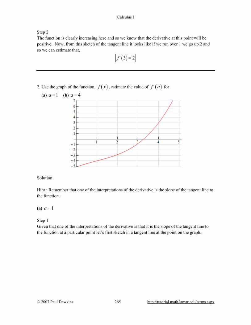
Calculus I
© 2007 Paul Dawkins 265 http://tutorial.math.lamar.edu/terms.aspx
Step 2 The function is clearly increasing here and so we know that the derivative at this point will be positive. Now, from this sketch of the tangent line it looks like if we run over 1 we go up 2 and so we can estimate that,
( )3 2f ′ =
2. Use the graph of the function, ( )f x , estimate the value of ( )f a′ for
(a) 1a = (b) 4a =
Solution Hint : Remember that one of the interpretations of the derivative is the slope of the tangent line to the function. (a) 1a = Step 1 Given that one of the interpretations of the derivative is that it is the slope of the tangent line to the function at a particular point let’s first sketch in a tangent line at the point on the graph.
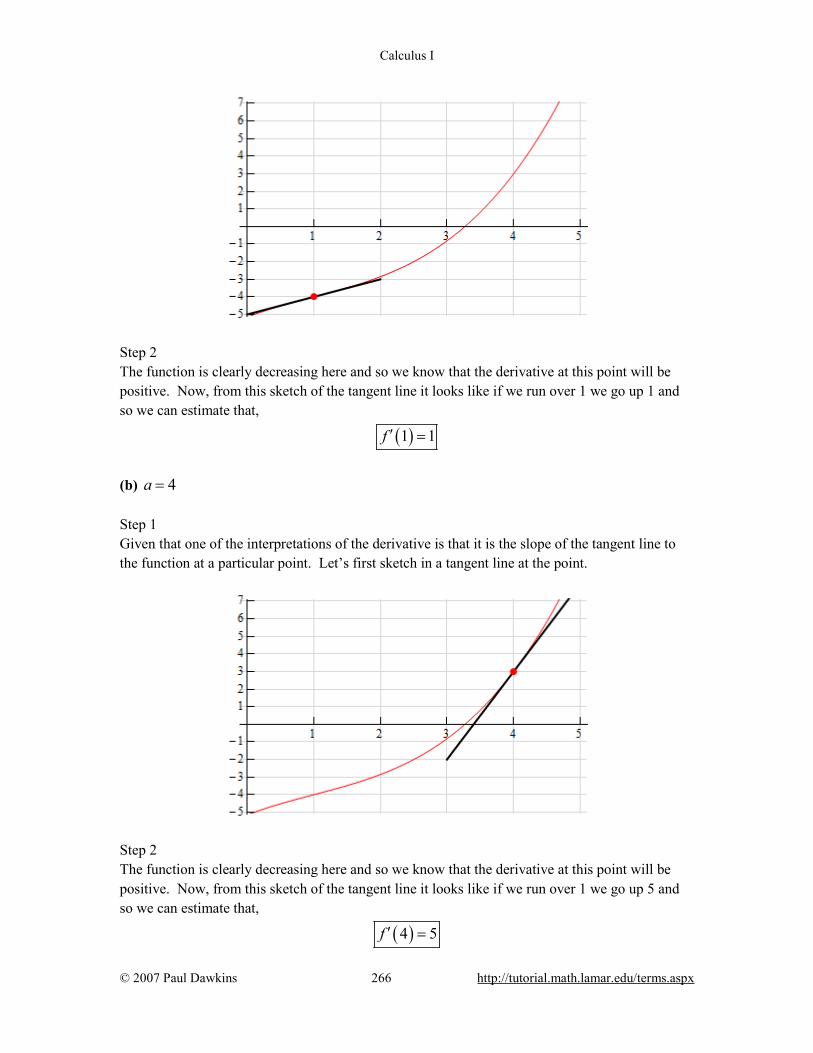
Calculus I
© 2007 Paul Dawkins 266 http://tutorial.math.lamar.edu/terms.aspx
Step 2 The function is clearly decreasing here and so we know that the derivative at this point will be positive. Now, from this sketch of the tangent line it looks like if we run over 1 we go up 1 and so we can estimate that,
( )1 1f ′ =
(b) 4a = Step 1 Given that one of the interpretations of the derivative is that it is the slope of the tangent line to the function at a particular point. Let’s first sketch in a tangent line at the point.
Step 2 The function is clearly decreasing here and so we know that the derivative at this point will be positive. Now, from this sketch of the tangent line it looks like if we run over 1 we go up 5 and so we can estimate that,
( )4 5f ′ =

Calculus I
© 2007 Paul Dawkins 267 http://tutorial.math.lamar.edu/terms.aspx
3. Sketch the graph of a function that satisfies ( )1 3f = , ( )1 1f ′ = , ( )4 5f = , ( )4 2f ′ = − . Solution Hint : Remember that one of the interpretations of the derivative is the slope of the tangent line to the function. Step 1 First, recall that one of the interpretations of the derivative is that it is the slope of the tangent line to the function at a particular point. So, let’s start off with a graph that has the given points on it and a sketch of a tangent line at the points whose slope is the value of the derivative at the points.
Step 2 Now, all that we need to do is sketch in a graph that goes through the indicated points and at the same time it must be parallel to the tangents that we sketched. There are many possible sketches that we can make here and so don’t worry if your sketch is not the same as the one here. This is just one possible sketch that meets the given conditions.
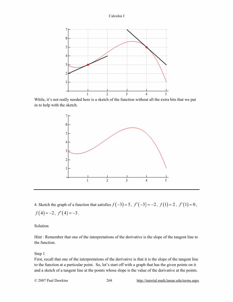
Calculus I
© 2007 Paul Dawkins 268 http://tutorial.math.lamar.edu/terms.aspx
While, it’s not really needed here is a sketch of the function without all the extra bits that we put in to help with the sketch.
4. Sketch the graph of a function that satisfies ( )3 5f − = , ( )3 2f ′ − = − , ( )1 2f = , ( )1 0f ′ = ,
( )4 2f = − , ( )4 3f ′ = − . Solution Hint : Remember that one of the interpretations of the derivative is the slope of the tangent line to the function. Step 1 First, recall that one of the interpretations of the derivative is that it is the slope of the tangent line to the function at a particular point. So, let’s start off with a graph that has the given points on it and a sketch of a tangent line at the points whose slope is the value of the derivative at the points.
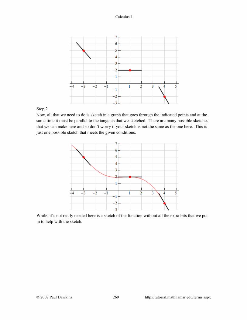
Calculus I
© 2007 Paul Dawkins 269 http://tutorial.math.lamar.edu/terms.aspx
Step 2 Now, all that we need to do is sketch in a graph that goes through the indicated points and at the same time it must be parallel to the tangents that we sketched. There are many possible sketches that we can make here and so don’t worry if your sketch is not the same as the one here. This is just one possible sketch that meets the given conditions.
While, it’s not really needed here is a sketch of the function without all the extra bits that we put in to help with the sketch.
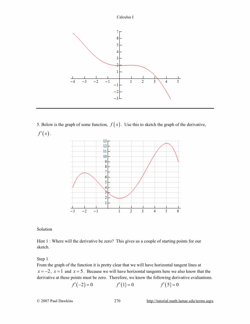
Calculus I
© 2007 Paul Dawkins 270 http://tutorial.math.lamar.edu/terms.aspx
5. Below is the graph of some function, ( )f x . Use this to sketch the graph of the derivative,
( )f x′ .
Solution Hint 1 : Where will the derivative be zero? This gives us a couple of starting points for our sketch. Step 1 From the graph of the function it is pretty clear that we will have horizontal tangent lines at
2x = − , 1x = and 5x = . Because we will have horizontal tangents here we also know that the derivative at these points must be zero. Therefore, we know the following derivative evaluations. ( ) ( ) ( )2 0 1 0 5 0f f f′ ′ ′− = = =
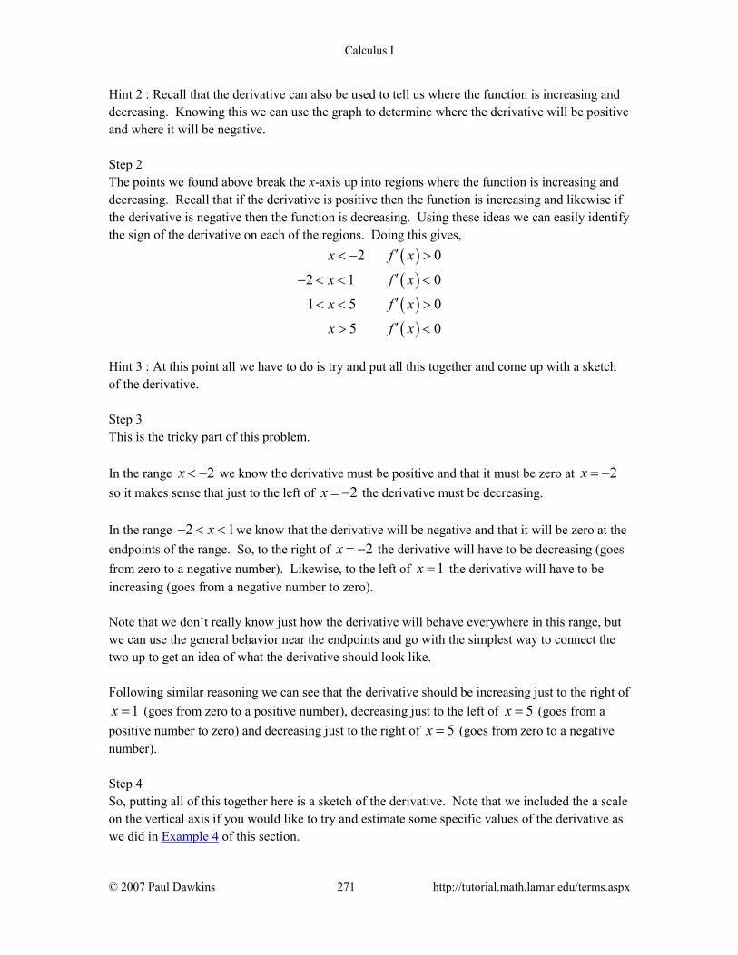
Calculus I
© 2007 Paul Dawkins 271 http://tutorial.math.lamar.edu/terms.aspx
Hint 2 : Recall that the derivative can also be used to tell us where the function is increasing and decreasing. Knowing this we can use the graph to determine where the derivative will be positive and where it will be negative. Step 2 The points we found above break the x-axis up into regions where the function is increasing and decreasing. Recall that if the derivative is positive then the function is increasing and likewise if the derivative is negative then the function is decreasing. Using these ideas we can easily identify the sign of the derivative on each of the regions. Doing this gives,
( )( )( )( )
2 0
2 1 0
1 5 0
5 0
x f x
x f x
x f x
x f x
′< − >
′− < < <
′< < >
′> <
Hint 3 : At this point all we have to do is try and put all this together and come up with a sketch of the derivative. Step 3 This is the tricky part of this problem. In the range 2x < − we know the derivative must be positive and that it must be zero at 2x = − so it makes sense that just to the left of 2x = − the derivative must be decreasing. In the range 2 1x− < < we know that the derivative will be negative and that it will be zero at the endpoints of the range. So, to the right of 2x = − the derivative will have to be decreasing (goes from zero to a negative number). Likewise, to the left of 1x = the derivative will have to be increasing (goes from a negative number to zero). Note that we don’t really know just how the derivative will behave everywhere in this range, but we can use the general behavior near the endpoints and go with the simplest way to connect the two up to get an idea of what the derivative should look like. Following similar reasoning we can see that the derivative should be increasing just to the right of
1x = (goes from zero to a positive number), decreasing just to the left of 5x = (goes from a positive number to zero) and decreasing just to the right of 5x = (goes from zero to a negative number). Step 4 So, putting all of this together here is a sketch of the derivative. Note that we included the a scale on the vertical axis if you would like to try and estimate some specific values of the derivative as we did in Example 4 of this section.

Calculus I
© 2007 Paul Dawkins 272 http://tutorial.math.lamar.edu/terms.aspx
6. Below is the graph of some function, ( )f x . Use this to sketch the graph of the derivative,
( )f x′ .
Solution Hint 1 : Because the derivative of a function is also the slope of the tangent line. We can therefore determine actual values of the derivative at almost every spot. Step 1 Because the three portions of the function are actually lines and the tangent line to a line would just be the line itself we can easily compute the derivative on each portion of the curve. On each of the portions we can use the grid included on the graph to compute the slope of each part. Knowing the slope of the graph on each portion will in turn tell us the slope of the tangent line for each portion. This in turn tells us that the derivative on each of the three portions is then,

Calculus I
© 2007 Paul Dawkins 273 http://tutorial.math.lamar.edu/terms.aspx
( )
( )
( )
1 121 23
2 2
x f x
x f x
x f x
′< − = −
′− < < =
′> = −
Hint 2 : What is the derivative at the “sharp points”? Step 2 Recall Example 4 from the previous section. In that example we showed that the derivative of the absolute value function does not exist at 0x = . The limit on the left side of 0x = (which gives the slope of the line on the left) and the limit on the right side of 0x = (which gives the slope of the line on the right) were different and so the overall limit did not exist. This in turn tells us that the derivative doesn’t exist at that point. Here we have the same problem. We’ll leave it to you to verify that the right and left handed limits at 1x = − are not the same and so the derivative does not exist at 1x = − . Likewise, the derivative does not exist at 2x = . There will therefore be open dots on the graph at these two points. Step 3 Here is the sketch of the derivative of this function.
7. Answer the following questions about the function ( ) 24 9W z z z= − .
(a) Is the function increasing or decreasing at 1z = − ? (b) Is the function increasing or decreasing at 2z = ? (c) Does the function ever stop changing? If yes, at what value(s) of z does the

Calculus I
© 2007 Paul Dawkins 274 http://tutorial.math.lamar.edu/terms.aspx
function stop changing? (a) Is the function increasing or decreasing at 1z = − ? We know that the derivative of a function gives us the rate of change of the function and so we’ll first need the derivative of this function. We computed this derivative in Problem 5 from the previous section and so we won’t show the work here. If you need the practice you should go back and redo that problem before proceeding. So, from our previous work we know that the derivative is, ( ) 8 9W z z′ = − Now all that we need to do is to compute : ( )1 17W ′ − = − . This is negative and so we know that
the function must be decreasing at 1z = − . (b) Is the function increasing or decreasing at 2z = ? Again, all we need to do is compute a derivative and since we’ve got the derivative written down in the first part there’s no reason to redo that here. The evaluation is : ( )2 7W ′ = . This is positive and so we know that the function must be
increasing at 2z = . (c) Does the function ever stop changing? If yes, at what value(s) of z does the function stop changing? Here all that we’re really asking is if the derivative is ever zero. So we need to solve,
( ) 90 8 9 08
W z z z′ = → − = ⇒ =
So, the function will stop changing at 98
z = .
8. What is the equation of the tangent line to ( ) 3 14f x x= − at 8x = .
Solution We know that the derivative of a function gives us the slope of the tangent line and so we’ll first need the derivative of this function. We computed this derivative in Problem 2 from the previous
Calculus I
© 2007 Paul Dawkins 275 http://tutorial.math.lamar.edu/terms.aspx
section and so we won’t show the work here. If you need the practice you should go back and redo that problem before proceeding. Note that we did use a different set of letters in the previous problem, but the work is identical. So, from our previous work (with a corresponding change of variables) we know that the derivative is, ( ) 14f x′ = − This tells us that the slope of the tangent line at 8x = is then : ( )8 14m f ′= = − . We also know
that a point on the tangent line is : ( )( ) ( )8, 8 8, 109f = − .
The tangent line is then, ( )109 14 8 3 14y x x= − − − = − Note that, in this case the tangent is the same as the function. This should not be surprising however as the function is a line and so any tangent line (i.e. parallel line) will in fact be the same as the line itself.
9. The position of an object at any time t is given by ( ) 14
ts tt
+=
+.
(a) Determine the velocity of the object at any time t. (b) Does the object ever stop moving? If yes, at what time(s) does the object stop moving? (a) Determine the velocity of the object at any time t. We know that the derivative of a function gives is the velocity of the object and so we’ll first need the derivative of this function. We computed this derivative in Problem 9 from the previous section and so we won’t show the work here. If you need the practice you should go back and redo that problem before proceeding. Note that we did use a different letter for the function in the previous problem, but the work is identical. So, from our previous work we know that the derivative is,
( )( )2
34
s tt
′ =+
(b) Does the object ever stop moving? If yes, at what time(s) does the object stop moving?

Calculus I
© 2007 Paul Dawkins 276 http://tutorial.math.lamar.edu/terms.aspx
We know that the object will stop moving if the velocity (i.e. the derivative) is zero. In this case the derivative is a rational expression and clearly the numerator will never be zero. Therefore, the derivative will not be zero and therefore the object never stops moving.
10. What is the equation of the tangent line to ( ) 5f xx
= at 12
x = ?
Solution We know that the derivative of a function gives us the slope of the tangent line and so we’ll first need the derivative of this function. We computed this derivative in Problem 8 from the previous section and so we won’t show the work here. If you need the practice you should go back and redo that problem before proceeding. Note that we did use a different set of letters in the previous problem, but the work is identical. So, from our previous work (with a corresponding change of variables) we know that the derivative is,
( ) 2
5f xx
′ = −
This tells us that the slope of the tangent line at 12
x = is then : 1 202
m f ′= = −
. We also
know that a point on the tangent line is : 1 1 1, ,102 2 2
f = .
The tangent line is then,
110 20 20 202
y x x = − − = −
11. Determine where, if anywhere, the function ( ) 3 22 1g x x x x= − + − stops changing.
Solution We know that the derivative of a function gives us the rate of change of the function and so we’ll first need the derivative of this function. We computed this derivative in Problem 7 from the previous section and so we won’t show the work here. If you need the practice you should go back and redo that problem before proceeding.

Calculus I
© 2007 Paul Dawkins 277 http://tutorial.math.lamar.edu/terms.aspx
From our previous work (with a corresponding change of variables) we know that the derivative is, ( ) 23 4 1g x x x′ = − + If the function stops changing at a point then the derivative will be zero at that point. So, to determine if we function stops changing we will need to solve,
( )
( ) ( )
2
0
3 4 1 013 1 1 0 , 13
g x
x x
x x x x
′ =
− + =
− − = ⇒ = =
So, the function will stop changing at 13
x = and 1x = .
12. Determine if the function ( ) 3 4Z t t= − increasing or decreasing at the given points.
(a) 5t = (b) 10t = (c) 300t = (a) 5t = We know that the derivative of a function gives us the rate of change of the function and so we’ll first need the derivative of this function. We computed this derivative in Problem 10 from the previous section and so we won’t show the work here. If you need the practice you should go back and redo that problem before proceeding. So, from our previous work we know that the derivative is,
( ) 32 3 4
Z tt
′ =−
Now all that we need to do is to compute : ( ) 352 11
Z ′ = . This is positive and so we know that
the function must be increasing at 5t = . (b) 10t = Again, all we need to do is compute a derivative and since we’ve got the derivative written down in the first part there’s no reason to redo that here.
Calculus I
© 2007 Paul Dawkins 278 http://tutorial.math.lamar.edu/terms.aspx
The evaluation is : ( ) 3102 26
Z ′ = . This is positive and so we know that the function must be
increasing at 10t = . (c) 300t = Again, all we need to do is compute a derivative and since we’ve got the derivative written down in the first part there’s no reason to redo that here.
The evaluation is : ( ) 33002 896
Z ′ = . This is positive and so we know that the function must
be increasing at 300t = . Final Note As a final note to all the parts of this problem let’s notice that we did not really need to do any evaluations. Because we know that square roots will always be positive it is clear that the derivative will always be positive regardless of the value of t we plug in. 13. Suppose that the volume of water in a tank for 0 6t≤ ≤ is given by ( ) 210 5Q t t t= + − .
(a) Is the volume of water increasing or decreasing at 0t = ? (b) Is the volume of water increasing or decreasing at 6t = ? (c) Does the volume of water ever stop changing? If yes, at what times(s) does the volume stop changing? (a) Is the volume of water increasing or decreasing at 0t = ? We know that the derivative of a function gives us the rate of change of the function and so we’ll first need the derivative of this function. We computed this derivative in Problem 4 from the previous section and so we won’t show the work here. If you need the practice you should go back and redo that problem before proceeding. So, from our previous work we know that the derivative is, ( ) 5 2Q t t′ = − Now all that we need to do is to compute : ( )0 5Q′ = . This is positive and so we know that the
volume of water in the tank must be increasing at 0t = . (b) Is the volume of water increasing or decreasing at 6t = ?
Calculus I
© 2007 Paul Dawkins 279 http://tutorial.math.lamar.edu/terms.aspx
Again, all we need to do is compute a derivative and since we’ve got the derivative written down in the first part there’s no reason to redo that here. The evaluation is : ( )6 7Q′ = − . This is negative and so we know that the volume of water in the
tank must be decreasing at 6t = . (c) Does the volume of water ever stop changing? If yes, at what times(s) does the volume stop changing? Here all that we’re really asking is if the derivative is ever zero. So we need to solve,
( ) 50 5 2 02
Q t t t′ = → − = ⇒ =
So, the volume of water will stop changing at 52
.
Differentiation Formulas 1. Find the derivative of ( ) 36 9 4f x x x= − + .
Solution There isn’t much to do here other than take the derivative using the rules we discussed in this section.
( ) 218 9f x x′ = − 2. Find the derivative of 4 22 10 13y t t t= − + . Solution There isn’t much to do here other than take the derivative using the rules we discussed in this section.
Calculus I
© 2007 Paul Dawkins 280 http://tutorial.math.lamar.edu/terms.aspx
38 20 13dy t tdt
= − +
3. Find the derivative of ( ) 7 74 3 9g z z z z−= − + .
Solution There isn’t much to do here other than take the derivative using the rules we discussed in this section.
( ) 6 828 21 9g z z z−′ = + + 4. Find the derivative of ( ) 4 3 29 8 12h y y y y− − −= − + + .
Solution There isn’t much to do here other than take the derivative using the rules we discussed in this section.
( ) 5 4 34 27 16h y y y y− − −′ = − + −
5. Find the derivative of 3 48 2y x x x= + − . Solution There isn’t much to do here other than take the derivative using the rules we discussed in this section. Remember that you’ll need to convert the roots to fractional exponents before you start taking the derivative. Here is the rewritten function.
11 132 48 2y x x x= + −
The derivative is,
21 332 41 8 1
2 3 2dy x x xdx
−− −= + −

Calculus I
© 2007 Paul Dawkins 281 http://tutorial.math.lamar.edu/terms.aspx
6. Find the derivative of ( ) 5 33 7 810 6 3f x x x x= − + − .
Solution There isn’t much to do here other than take the derivative using the rules we discussed in this section. Remember that you’ll need to convert the roots to fractional exponents before you start taking the derivative. Here is the rewritten function.
( ) ( ) ( ) ( )3 871 1 1
3 7 8 5 325 2 310 6 3 10 6 3f x x x x x x x= − + − = − + − The derivative is,
( )2 5 2 55 55 3 5 32 23 7 8 710 6 6 16
5 2 3 2f x x x x x x x
− − ′ = − + = − +
7. Find the derivative of ( ) 3 5
4 1 86
f tt t t
= − + .
Solution There isn’t much to do here other than take the derivative using the rules we discussed in this section. Remember that you’ll need to rewrite the terms so that each of the t’s are in the numerator with negative exponents before taking the derivative. Here is the rewritten function.
( ) 1 3 514 86
f t t t t− − −= − +
The derivative is,
( ) 2 4 614 402
f t t t t− − −′ = − + −

Calculus I
© 2007 Paul Dawkins 282 http://tutorial.math.lamar.edu/terms.aspx
8. Find the derivative of ( ) 4 103
6 1 18 3
R zz zz
= + − .
Solution There isn’t much to do here other than take the derivative using the rules we discussed in this section. Remember that you’ll need to rewrite the terms so that each of the z’s are in the numerator with negative exponents and rewrite the root as a fractional exponent before taking the derivative. Here is the rewritten function.
( )3
4 102 1 168 3
R z z z z− − −= + −
The derivative is,
( ) ( ) ( )5 5
5 11 5 112 23 1 1 1 106 4 10 92 8 3 2 3
R z z z z z z z− −− − − − ′ = − + − − − = − − +
9. Find the derivative of ( )23 9z x x= − .
Solution There isn’t much to do here other than take the derivative using the rules we discussed in this section. Remember that in order to do this derivative we’ll first need to multiply the function out before we take the derivative. Here is the rewritten function. 33 9z x x= − The derivative is,
29 9dz xdx
= −
10. Find the derivative of ( ) ( )( )24 2g y y y y= − + .
Solution

Calculus I
© 2007 Paul Dawkins 283 http://tutorial.math.lamar.edu/terms.aspx
There isn’t much to do here other than take the derivative using the rules we discussed in this section. Remember that in order to do this derivative we’ll first need to multiply the function out before we take the derivative. Here is the rewritten function. ( ) 3 22 8g y y y y= − − The derivative is,
( ) 23 4 8g y y y′ = − −
11. Find the derivative of ( )34 7 8x xh x
x− +
= .
Solution There isn’t much to do here other than take the derivative using the rules we discussed in this section. Remember that in order to do this derivative we’ll first need to divide the function out and simplify before we take the derivative. Here is the rewritten function.
( )3
2 14 7 8 4 7 8x xh x x xx x x
−= − + = − +
The derivative is,
( ) 28 8h x x x−′ = −
12. Find the derivative of ( )5 3
3
5 2y y yf yy
− += .
Solution There isn’t much to do here other than take the derivative using the rules we discussed in this section. Remember that in order to do this derivative we’ll first need to divide the function out and simplify before we take the derivative. Here is the rewritten function.
Calculus I
© 2007 Paul Dawkins 284 http://tutorial.math.lamar.edu/terms.aspx
( )5 3
2 23 3 3
5 2 5 2y y yf y y yy y y
−= − + = − +
The derivative is,
( ) 32 4f y y y−′ = − 13. Determine where, if anywhere, the function ( ) 3 29 48 2f x x x x= + − + is not changing.
Hint : Recall the various interpretations of the derivative. One of them is exactly what we need to do this problem. Solution Step 1 Recall that one of the interpretations of the derivative is that it gives the rate of change of the function. So, the function won’t be changing if its rate of change is zero and so all we need to do is find the derivative and set it equal to zero to determine where the rate of change is zero and hence the function will not be changing. First the derivative, and we’ll do a little factoring while we are at it.
( ) ( ) ( ) ( )2 23 18 48 3 6 16 3 8 2f x x x x x x x′ = + − = + − = + − Step 2 Now all that we need to do is set this equation to zero and solve. ( ) ( ) ( )0 3 8 2 0f x x x′ = ⇒ + − = We can easily see from this that the derivative will be zero at 8x = − and 2x = . The function therefore not be changing at,
8 and 2x x= − = 14. Determine where, if anywhere, the function 4 3 22 3y z z z= − − is not changing. Hint : Recall the various interpretations of the derivative. One of them is exactly what we need to do this problem.
Calculus I
© 2007 Paul Dawkins 285 http://tutorial.math.lamar.edu/terms.aspx
Solution Step 1 Recall that one of the interpretations of the derivative is that it gives the rate of change of the function. So, the function won’t be changing if its rate of change is zero and so all we need to do is find the derivative and set it equal to zero to determine where the rate of change is zero and hence the function will not be changing. First the derivative, and we’ll do a little factoring while we are at it.
( )3 2 28 3 6 8 3 6dy z z z z z zdz
= − − = − −
Step 2 Now all that we need to do is set this equation to zero and solve.
( )2 2
0
8 3 6 0 0, 8 3 6 0
dydz
z z z z z z
=
− − = → = − − =
We can easily see from this that the derivative will be zero at 0z = , however, because the quadratic doesn’t factor we’ll need to use the quadratic formula to determine where, if anywhere, that will be zero.
( ) ( ) ( )
( )
23 3 4 8 6 3 2012 8 16
z± − − − ±
= =
The function therefore not be changing at,
3 201 3 2010 1.07359 0.6985916 16
z z z+ −= = = = = −
15. Find the tangent line to ( ) 16 4g x xx
= − at 4x = .
Hint : Recall the various interpretations of the derivative. One of them will help us do this problem. Solution Step 1

Calculus I
© 2007 Paul Dawkins 286 http://tutorial.math.lamar.edu/terms.aspx
Recall that one of the interpretations of the derivative is that it gives slope of the tangent line to the graph of the function. So, we’ll need the derivative of the function. However before doing that we’ll need to do a little rewrite. Here is that work as well as the derivative.
( ) ( )1 1
1 22 22
16 216 4 16 2g x x x g x x xx x
−− −′= − ⇒ = − − = − −
Note that we rewrote the derivative back into rational expressions with roots to help with the evaluation. Step 2 Next we need to evaluate the function and derivative at 4x = .
( ) ( ) 2
16 16 24 4 4 4 4 24 4 4
g g′= − = − = − − −
Step 3 Now all that we need to do is write down the equation of the tangent line.
( ) ( ) ( ) ( )4 4 4 4 2 4 2 4y g g x x y x′= + − = − − − → = − + 16. Find the tangent line to ( ) 4 67 8 2f x x x x−= + + at 1x = − .
Hint : Recall the various interpretations of the derivative. One of them will help us do this problem. Solution Step 1 Recall that one of the interpretations of the derivative is that it gives slope of the tangent line to the graph of the function. So, we’ll need the derivative of the function.
( ) 3 7 37
4828 48 2 28 2f x x x xx
−′ = − + = − +
Note that we rewrote the derivative back into rational expressions help a little with the evaluation. Step 2

Calculus I
© 2007 Paul Dawkins 287 http://tutorial.math.lamar.edu/terms.aspx
Next we need to evaluate the function and derivative at 1x = − .
( ) ( )1 7 8 2 13 1 28 48 2 22f f ′− = + − = − = − + + = Step 3 Now all that we need to do is write down the equation of the tangent line.
( ) ( )( ) ( )1 1 1 13 22 1 22 35y f f x x y x′= − + − + = + + → = + 17. The position of an object at any time t is given by ( ) 4 3 23 40 126 9s t t t t= − + − .
(a) Determine the velocity of the object at any time t. (b) Does the object ever stop changing? (c) When is the object moving to the right and when is the object moving to the left? Solution Hint : Recall the various interpretations of the derivative. One of them is exactly what we need for this part. (a) Determine the velocity of the object at any time t. Recall that one of the interpretations of the derivative is that it gives the velocity of an object if we know the position function of the object. We’ve been given the position function of the object and so all we need to do is find its derivative and we’ll have the velocity of the object at any time t. The velocity of the object is then,
( ) ( )( )3 212 120 252 12 3 7s t t t t t t t′ = − + = − − Note that the derivative was factored for later parts and doesn’t really need to be done in general. Hint : If the object isn’t moving what is the velocity? (b) Does the object ever stop changing? The object will not be moving if the velocity is ever zero and so all we need to do is set the derivative equal to zero and solve. ( ) ( ) ( )0 12 3 7 0s t t t t′ = ⇒ − − =
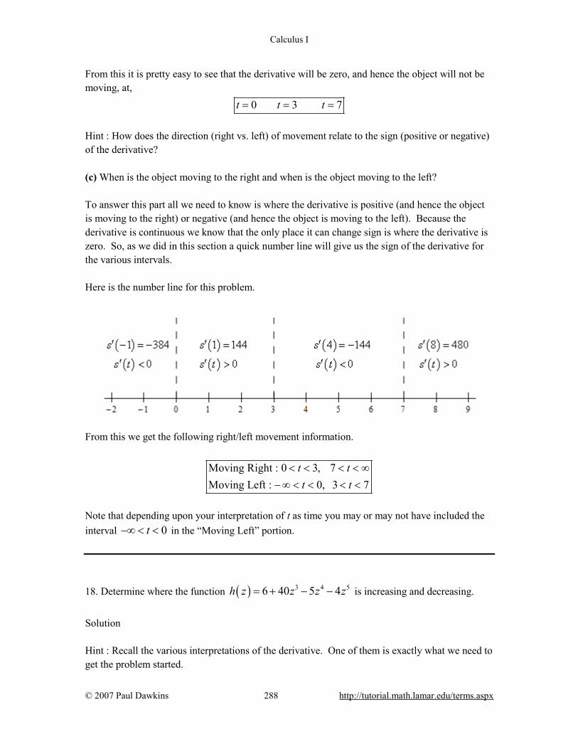
Calculus I
© 2007 Paul Dawkins 288 http://tutorial.math.lamar.edu/terms.aspx
From this it is pretty easy to see that the derivative will be zero, and hence the object will not be moving, at,
0 3 7t t t= = = Hint : How does the direction (right vs. left) of movement relate to the sign (positive or negative) of the derivative? (c) When is the object moving to the right and when is the object moving to the left? To answer this part all we need to know is where the derivative is positive (and hence the object is moving to the right) or negative (and hence the object is moving to the left). Because the derivative is continuous we know that the only place it can change sign is where the derivative is zero. So, as we did in this section a quick number line will give us the sign of the derivative for the various intervals. Here is the number line for this problem.
From this we get the following right/left movement information.
Moving Right : 0 3, 7Moving Left : 0, 3 7
t tt t
< < < < ∞− ∞ < < < <
Note that depending upon your interpretation of t as time you may or may not have included the interval 0t−∞ < < in the “Moving Left” portion. 18. Determine where the function ( ) 3 4 56 40 5 4h z z z z= + − − is increasing and decreasing.
Solution Hint : Recall the various interpretations of the derivative. One of them is exactly what we need to get the problem started.
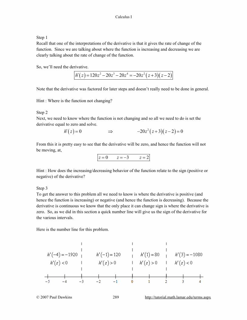
Calculus I
© 2007 Paul Dawkins 289 http://tutorial.math.lamar.edu/terms.aspx
Step 1 Recall that one of the interpretations of the derivative is that it gives the rate of change of the function. Since we are talking about where the function is increasing and decreasing we are clearly talking about the rate of change of the function. So, we’ll need the derivative.
( ) ( ) ( )2 3 4 2120 20 20 20 3 2h z z z z z z z′ = − − = − + − Note that the derivative was factored for later steps and doesn’t really need to be done in general. Hint : Where is the function not changing? Step 2 Next, we need to know where the function is not changing and so all we need to do is set the derivative equal to zero and solve. ( ) ( ) ( )20 20 3 2 0h z z z z′ = ⇒ − + − = From this it is pretty easy to see that the derivative will be zero, and hence the function will not be moving, at,
0 3 2z z z= = − = Hint : How does the increasing/decreasing behavior of the function relate to the sign (positive or negative) of the derivative? Step 3 To get the answer to this problem all we need to know is where the derivative is positive (and hence the function is increasing) or negative (and hence the function is decreasing). Because the derivative is continuous we know that the only place it can change sign is where the derivative is zero. So, as we did in this section a quick number line will give us the sign of the derivative for the various intervals. Here is the number line for this problem.
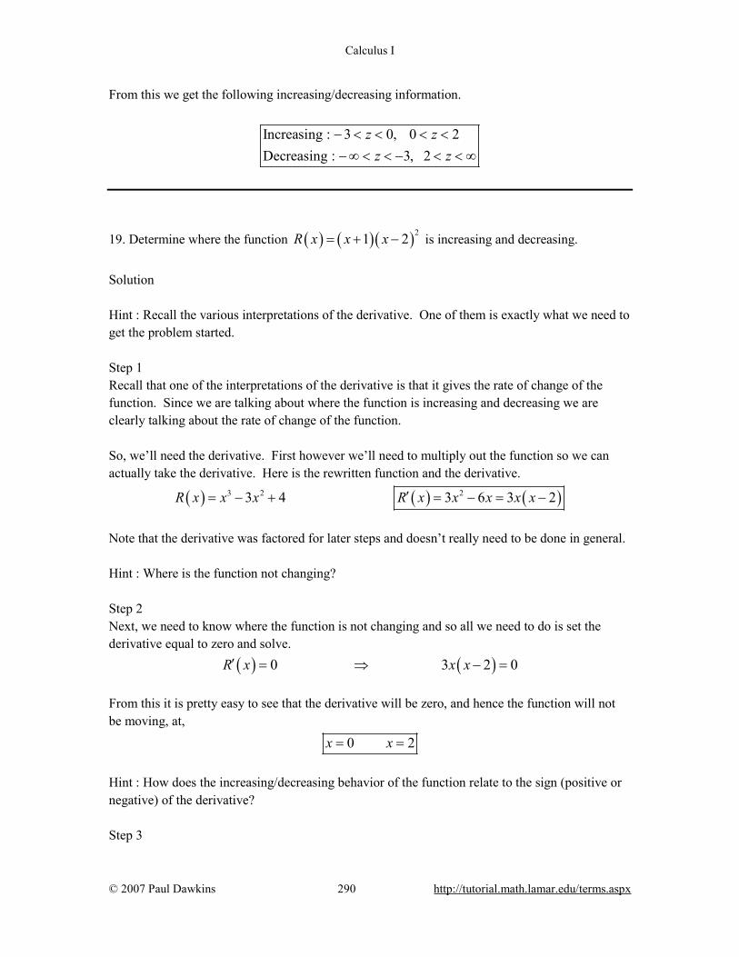
Calculus I
© 2007 Paul Dawkins 290 http://tutorial.math.lamar.edu/terms.aspx
From this we get the following increasing/decreasing information.
Increasing : 3 0, 0 2Decreasing : 3, 2
z zz z
− < < < <− ∞ < < − < < ∞
19. Determine where the function ( ) ( ) ( )21 2R x x x= + − is increasing and decreasing.
Solution Hint : Recall the various interpretations of the derivative. One of them is exactly what we need to get the problem started. Step 1 Recall that one of the interpretations of the derivative is that it gives the rate of change of the function. Since we are talking about where the function is increasing and decreasing we are clearly talking about the rate of change of the function. So, we’ll need the derivative. First however we’ll need to multiply out the function so we can actually take the derivative. Here is the rewritten function and the derivative.
( ) ( ) ( )3 2 23 4 3 6 3 2R x x x R x x x x x′= − + = − = − Note that the derivative was factored for later steps and doesn’t really need to be done in general. Hint : Where is the function not changing? Step 2 Next, we need to know where the function is not changing and so all we need to do is set the derivative equal to zero and solve. ( ) ( )0 3 2 0R x x x′ = ⇒ − = From this it is pretty easy to see that the derivative will be zero, and hence the function will not be moving, at,
0 2x x= = Hint : How does the increasing/decreasing behavior of the function relate to the sign (positive or negative) of the derivative? Step 3

Calculus I
© 2007 Paul Dawkins 291 http://tutorial.math.lamar.edu/terms.aspx
To get the answer to this problem all we need to know is where the derivative is positive (and hence the function is increasing) or negative (and hence the function is decreasing). Because the derivative is continuous we know that the only place it can change sign is where the derivative is zero. So, as we did in this section a quick number line will give us the sign of the derivative for the various intervals. Here is the number line for this problem.
From this we get the following increasing/decreasing information.
Increasing : 0, 2Decreasing : 0 2
x zz
− ∞ < < < < ∞< <
20. Determine where, if anywhere, the tangent line to ( ) 3 25f x x x x= − + is parallel to the line
4 23y x= + . Solution Step 1 The first thing that we’ll need of course is the slope of the tangent line. So, all we need to do is take the derivative of the function.
( ) 23 10 1f x x x′ = − + Hint : What is the relationship between the slope of two parallel lines? Step 2 Two lines that are parallel will have the same slope and so all we need to do is determine where the slope of the tangent line will be 4, the slope of the given line. In other words, we’ll need to solve,
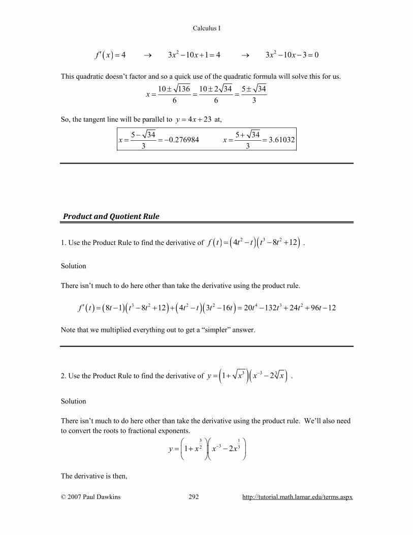
Calculus I
© 2007 Paul Dawkins 292 http://tutorial.math.lamar.edu/terms.aspx
( ) 2 24 3 10 1 4 3 10 3 0f x x x x x′ = → − + = → − − = This quadratic doesn’t factor and so a quick use of the quadratic formula will solve this for us.
10 136 10 2 34 5 346 6 3
x ± ± ±= = =
So, the tangent line will be parallel to 4 23y x= + at,
5 34 5 340.276984 3.610323 3
x x− += = − = =
Product and Quotient Rule
1. Use the Product Rule to find the derivative of ( ) ( )( )2 3 24 8 12f t t t t t= − − + .
Solution There isn’t much to do here other than take the derivative using the product rule.
( ) ( ) ( ) ( )( )3 2 2 2 4 3 28 1 8 12 4 3 16 20 132 24 96 12f t t t t t t t t t t t t′ = − − + + − − = − + + − Note that we multiplied everything out to get a “simpler” answer.
2. Use the Product Rule to find the derivative of ( )( )3 3 31 2y x x x−= + − .
Solution There isn’t much to do here other than take the derivative using the product rule. We’ll also need to convert the roots to fractional exponents.
13
3 321 2y x x x− = + −
The derivative is then,
Calculus I
© 2007 Paul Dawkins 293 http://tutorial.math.lamar.edu/terms.aspx
1 2 2 51 3 5
3 4 43 3 3 62 2 23 2 3 2 112 1 3 32 3 2 3 3
dy x x x x x x x x x xdx
− −−− − − = − + + − − = − − − −
Note that we multiplied everything out to get a “simpler” answer.
3. Use the Product Rule to find the derivative of ( ) ( )( )2 2 31 2 3 5 8h z z z z z z= + + + − .
Solution There isn’t much to do here other than take the derivative using the product rule.
( ) ( ) ( ) ( ) ( )2 3 2 2
2 3 4
2 6 5 8 1 2 3 5 16 3
5 36 90 88 15
h z z z z z z z z z
z z z z
′ = + + − + + + + −
= + + + −
Note that we multiplied everything out to get a “simpler” answer.
4. Use the Quotient Rule to find the derivative of ( )26
2xg x
x=
− .
Solution There isn’t much to do here other than take the derivative using the quotient rule.
( ) ( ) ( )( ) ( )
2 2
2 2
12 2 6 1 24 62 2
x x x x xg xx x
− − − −′ = =− −
5. Use the Quotient Rule to find the derivative of ( )4
2
32 1w wR ww
+=
+ .
Solution There isn’t much to do here other than take the derivative using the quotient rule.
Calculus I
© 2007 Paul Dawkins 294 http://tutorial.math.lamar.edu/terms.aspx
( ) ( )( ) ( ) ( )( ) ( )
3 2 4 5 3 2
2 22 2
3 4 2 1 3 4 4 4 6 3
2 1 2 1
w w w w w w w wR ww w
+ + − + + − +′ = =+ +
6. Use the Quotient Rule to find the derivative of ( ) 2
27 4
x xf xx x
+=
− .
Solution There isn’t much to do here other than take the derivative using the quotient rule.
( )( )( ) ( )( )
( )
1 121 2 22
22
7 4 7 82 27 4
x x xx x xf xx x
− − − −+ +′ =−
7. If ( )2 8f = − , ( )2 3f ′ = , ( )2 17g = and ( )2 4g′ = − determine the value of ( ) ( )2f g ′ .
Solution We know that the product rule is,
( ) ( ) ( ) ( ) ( ) ( )f g x f x g x f x g x′ ′ ′= + Now, we want to know the value of this at 2x = and so all we need to do is plug this into the derivative. Doing this gives,
( ) ( ) ( ) ( ) ( ) ( )2 2 2 2 2f g f g f g′ ′ ′= + Now, we were given values for all these quantities and so all we need to do is plug these into our “formula” above.
( ) ( ) ( )( ) ( ) ( )2 3 17 8 4 83f g ′ = + − − = 8. If ( ) ( )3f x x g x= , ( )7 2g − = , ( )7 9g′ − = − determine the value of ( )7f ′ − .

Calculus I
© 2007 Paul Dawkins 295 http://tutorial.math.lamar.edu/terms.aspx
Hint : Even though we don’t know what ( )g x is we can still use the product rule to take the
derivative and then we can use the given information to get the value of ( )7f ′ − .
Solution Even though we don’t know what ( )g x is we do have a product of two functions here and so we
can use the product rule to determine the derivative of ( )f x .
( ) ( ) ( )2 33f x x g x x g x′ ′= + Now all we need to do is plug 7x = − into this and use the given information to determine the value of ( )7f ′ − .
( ) ( ) ( ) ( ) ( ) ( ) ( ) ( )( )2 37 3 7 7 7 7 3 49 2 343 9 3381f g g′ ′− = − − + − − = + − − =
9. Find the equation of the tangent line to ( ) ( ) ( )21 12 4f x x x= + − at 9x = .
Solution Step 1 We know that the derivative of the function will give us the slope of the tangent line so we’ll need the derivative of the function. We’ll use the product rule to get the derivative.
( ) ( ) ( )( ) ( ) ( )1
2 22 66 4 1 12 2 4 2 1 12f x x x x x x x xx
− ′ = − + + − = − − +
Step 2 Note that we didn’t bother to “simplify” the derivative (other than converting the fractional exponent back to a root) because all we really need this for is a quick evaluation. Speaking of which here are the evaluations that we’ll need for this problem. ( ) ( )( ) ( ) ( ) ( ) ( )9 37 77 2849 9 2 77 18 37 820f f ′= − = − = − − = − Step 3 Now all that we need to do is write down the equation of the tangent line.
( ) ( )( ) ( )9 9 9 2849 820 9 820 4531y f f x x y x′= + − = − − − → = − +

Calculus I
© 2007 Paul Dawkins 296 http://tutorial.math.lamar.edu/terms.aspx
10. Determine where ( )2
21 8x xf x
x−
=+
is increasing and decreasing.
Solution Step 1 We’ll first need the derivative, which will require the quotient rule, because we know that the derivative will give us the rate of change of the function. Here is the derivative.
( )( ) ( ) ( )( )
( ) ( )
2 2 2
2 22 2
1 2 1 8 16 1 2 8
1 8 1 8
x x x x x x xf xx x
− + − − − −′ = =+ +
Step 2 Next, we need to know where the function is not changing and so all we need to do is set the derivative equal to zero and solve. In this case it is clear that the denominator will never be zero for any real number and so the derivative will only be zero where the numerator is zero. Therefore, setting the numerator equal to zero and solving gives,
( ) ( )( )2 21 2 8 8 2 1 4 1 2 1 0x x x x x x− − = − + − = − − + = From this it is pretty easy to see that the derivative will be zero, and hence the function will not be changing, at,
1 12 4
x x= − =
Step 3 To get the answer to this problem all we need to know is where the derivative is positive (and hence the function is increasing) or negative (and hence the function is decreasing). Because the derivative is continuous we know that the only place it can change sign is where the derivative is zero. So, as we did in this section a quick number line will give us the sign of the derivative for the various intervals. Here is the number line for this problem.

Calculus I
© 2007 Paul Dawkins 297 http://tutorial.math.lamar.edu/terms.aspx
From this we get the following increasing/decreasing information.
1 1Increasing :2 4
1 1Decreasing : ,2 4
x
x x
− < <
− ∞ < < − < < ∞
11. Determine where ( ) ( )( )2 24 1 5V t t t= − + is increasing and decreasing.
Solution Step 1 We’ll first need the derivative, for which we will use the product rule, because we know that the derivative will give us the rate of change of the function. Here is the derivative.
( ) ( ) ( ) ( )( ) ( )2 2 3 22 1 5 4 10 38 20 2 19 10V t t t t t t t t t′ = − + + − = − = −
Step 2 Next, we need to know where the function is not changing and so all we need to do is set the derivative equal to zero and solve. From the factored form of the derivative it is easy to see that the derivative will be zero at,
190 1.378410
t t= = ± = ±
Step 3 To get the answer to this problem all we need to know is where the derivative is positive (and hence the function is increasing) or negative (and hence the function is decreasing). Because the derivative is continuous we know that the only place it can change sign is where the derivative is

Calculus I
© 2007 Paul Dawkins 298 http://tutorial.math.lamar.edu/terms.aspx
zero. So, as we did in this section a quick number line will give us the sign of the derivative for the various intervals. Here is the number line for this problem.
From this we get the following increasing/decreasing information.
19 19Increasing : , 010 10
19 19Decreasing : 0,10 10
t t
t x
− ∞ < < − < <
− < < < < ∞
Derivatives of Trig Functions
1. Evaluate ( )
0
sin 10limz
zz→
.
Solution All we need to do is set this up to allow us to use the fact from the notes in this section.
( ) ( ) ( ) ( )0 0 0
sin 10 10sin 10 sin 10lim lim 10lim 10 1 10
10 10z z z
z z zz z z→ → →
= = = =
2. Evaluate ( )( )0
sin 12lim
sin 5α
αα→
.
Calculus I
© 2007 Paul Dawkins 299 http://tutorial.math.lamar.edu/terms.aspx
Solution All we need to do is set this up to allow us to use the fact from the notes in this section.
( )( )
( )( )
( )( )
( )( )
( )( )
( ) ( )
0 0 0
0 0 0
sin 12 12 sin 12 sin 125 12 5lim lim limsin 5 12 5 sin 5 5 12 sin 5
sin 12 sin 1212 5 12 5lim lim lim5 12 sin 5 5 12 sin 5
12 121 15 5
α α α
α α α
α α α αα α αα α α α α α α
α αα αα α α α
→ → →
→ → →
= =
= =
= =
3. Evaluate ( )
0
cos 4 1limx
xx→
− .
Solution All we need to do is set this up to allow us to use the fact from the notes in this section.
( ) ( )( ) ( ) ( )
0 0 0
4 cos 4 1cos 4 1 cos 4 1lim lim 4lim 4 0 0
4 4x x x
xx xx x x→ → →
−− −= = = =
4. Differentiate ( ) ( ) ( )2cos 6sec 3f x x x= − + .
Solution Not much to do here other than take the derivative. ( ) ( ) ( ) ( )2sin 6sec tanf x x x x′ = − − 5. Differentiate ( ) ( ) ( )10 tan 2cotg z z z= − .
Solution Not much to do here other than take the derivative.
Calculus I
© 2007 Paul Dawkins 300 http://tutorial.math.lamar.edu/terms.aspx
( ) ( ) ( )2 210sec 2cscg z z z′ = + 6. Differentiate ( ) ( ) ( )tan secf w w w= .
Solution Not much to do here other than take the derivative, which will require the product rule.
( ) ( ) ( ) ( ) ( ) ( ) ( ) ( ) ( )2 3 2sec sec tan sec tan sec sec tanf w w w w w w w w w′ = + = + 7. Differentiate ( ) ( )3 2 sinh t t t t= − .
Solution Not much to do here other than take the derivative, which will require the product rule for the second term. You’ll need to be careful with the minus sign on the second term. You can either use a set of parenthesis around the derivative of the second term or you can think of the minus sign as part of the “first” function. We’ll think of the minus sign as part of the first function for this problem.
( ) ( ) ( )2 23 2 sin cosh t t t t t t′ = − −
8. Differentiate ( )6 4 cscy x x= + .
Solution Not much to do here other than take the derivative, which will require the product rule for the second term.
( ) ( ) ( ) ( )( ) ( ) ( ) ( )1 1
1 2 224 csc 4 csc cos 2 csc 4 csc cosy x x x x x x x x x x
− −′ = + − = −
Calculus I
© 2007 Paul Dawkins 301 http://tutorial.math.lamar.edu/terms.aspx
9. Differentiate ( ) ( ) ( )1
2sin 4cosR t
t t=
− .
Solution Not much to do here other than take the derivative, which will require the quotient rule.
( ) ( ) ( ) ( )( ) ( ) ( ) ( )( )( ) ( )( )
( ) ( )( ) ( )( )2 2
0 2sin 4cos 1 2cos 4sin 2cos 4sin
2sin 4cos 2sin 4cos
t t t t t tR t
t t t t
− − + − −′ = =
− −
10. Differentiate ( ) ( )( )
tan1 cscv v
Z vv
+=
+ .
Solution Not much to do here other than take the derivative, which will require the quotient rule.
( )( )( ) ( )( ) ( )( ) ( ) ( )( )
( )( )( )( ) ( )( ) ( ) ( ) ( )( )
( )( )
2
2
2
2
1 sec 1 csc tan csc cot
1 csc
1 sec 1 csc csc cot tan
1 csc
v v v v v vZ v
v
v v v v v v
v
+ + − + −′ =
+
+ + + +=
+
11. Find the tangent line to ( ) ( ) ( )tan 9cosf x x x= + at x π= .
Solution Step 1 We know that the derivative of the function will give us the slope of the tangent line so we’ll need the derivative of the function. ( ) ( ) ( )2sec 9sinf x x x′ = − Step 2 Now all we need to do is evaluate the function and the derivative at the point in question.
Calculus I
© 2007 Paul Dawkins 302 http://tutorial.math.lamar.edu/terms.aspx
( ) ( ) ( ) ( ) ( ) ( )2tan 9cos 9 sec 9sin 1f fπ π π π π π′= + = − = − = Step 3 Now all that we need to do is write down the equation of the tangent line.
( ) ( ) ( ) ( ) ( )9 1 9y f f x x y xπ π π π π′= + − = − + − → = − + Don’t get excited about the presence of the π in the answer. It is just a number like the 9 is and so is nothing to worry about. 12. The position of an object is given by ( ) ( )2 7coss t t= + determine all the points where the
object is not moving. Solution We know that the object will not be moving if its velocity, which is simply the derivative of the position function, is not zero. So all we need to do is take the derivative, set it equal to zero and solve. ( ) ( ) ( )7sin 7sin 0s t t t′ = − ⇒ − = So, for this problem the object will not be moving anywhere that sine is zero. From our recollection of the unit circle we know that will be at,
0 2 2 and 2 0, 1, 2, 3,t n n t n nπ π π π= + = = + = ± ± ± … 13. Where in the range [ ]2,7− is the function ( ) ( )4cosf x x x= − is increasing and
decreasing. Solution Step 1 We’ll first need the derivative because we know that the derivative will give us the rate of change of the function. Here is the derivative.
( ) ( )4sin 1f x x′ = − −

Calculus I
© 2007 Paul Dawkins 303 http://tutorial.math.lamar.edu/terms.aspx
Step 2 Next, we need to know where the function is not changing and so all we need to do is set the derivative equal to zero and solve.
( ) ( ) 14sin 1 0 sin4
x x− − = ⇒ = −
A quick calculator computation tells us that,
1 1sin 0.25274
x − = − = −
Recalling our work in the Review chapter on solving trig equations we know that a positive angle corresponding to this solution is : 2 0.2527 6.0305x π= − = . Either can be used, but we will use the positive angle. Also, from a quick check on a unit circle we can see that 0.2527 3.3943x π= + = will be a second solution. Putting all of this together and we can see that the derivative will be zero at, 6.0305 2 and 3.3943 2 0, 1, 2, 3,x n x n nπ π= + = + = ± ± ± … Finally, all we need to so is plug in some n’s to determine which solutions fall in the interval we are working on, [ ]2,7− .
1: 0.2527 2.8889n x x= − = − = −
0 : 6.0305 3.39431: 12.3137
n x xn x
= = == = 9.6775x =
So, in the interval [ ]2,7− the function will stop changing at the following three points.
0.2527, 3.3943, 6.0305x = − Step 3 To get the answer to this problem all we need to know is where the derivative is positive (and hence the function is increasing) or negative (and hence the function is decreasing). Because the derivative is continuous we know that the only place it can change sign is where the derivative is zero. So, as we did in this section a quick number line will give us the sign of the derivative for the various intervals. Here is the number line for this problem.
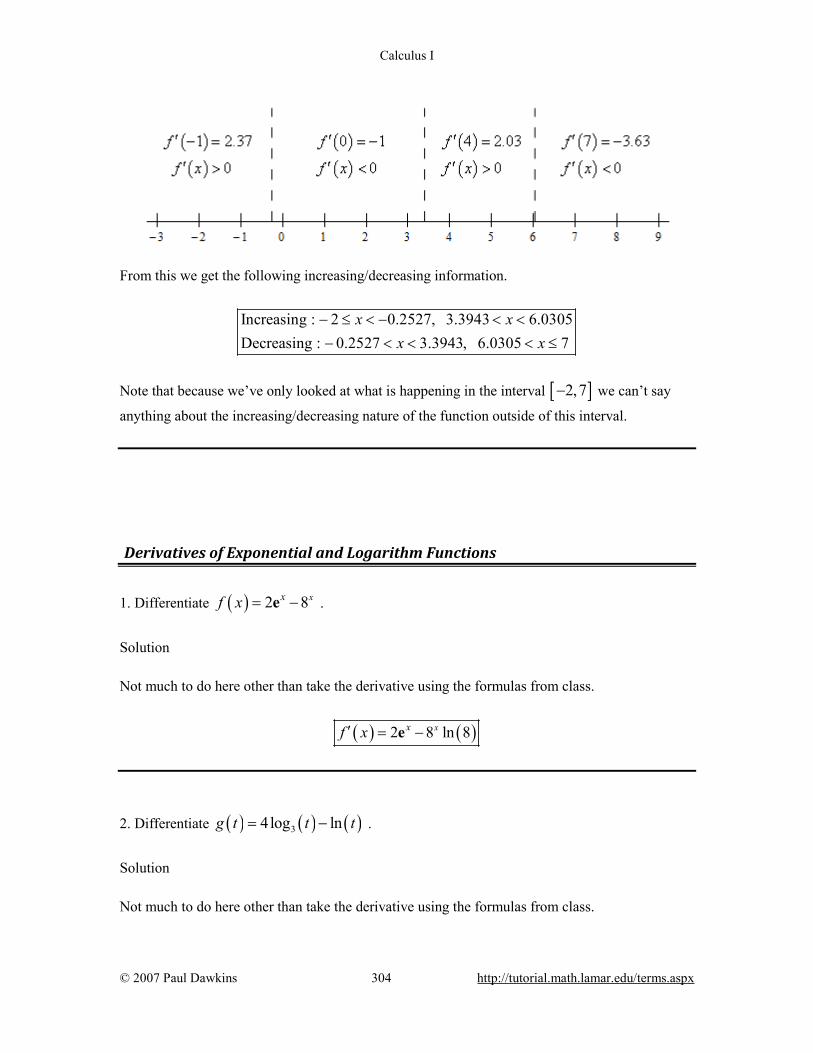
Calculus I
© 2007 Paul Dawkins 304 http://tutorial.math.lamar.edu/terms.aspx
From this we get the following increasing/decreasing information.
Increasing : 2 0.2527, 3.3943 6.0305Decreasing : 0.2527 3.3943, 6.0305 7
x xx x
− ≤ < − < <− < < < ≤
Note that because we’ve only looked at what is happening in the interval [ ]2,7− we can’t say
anything about the increasing/decreasing nature of the function outside of this interval.
Derivatives of Exponential and Logarithm Functions 1. Differentiate ( ) 2 8xxf x = −e .
Solution Not much to do here other than take the derivative using the formulas from class.
( ) ( )2 8 ln 8xxf x′ = −e 2. Differentiate ( ) ( ) ( )34log lng t t t= − .
Solution Not much to do here other than take the derivative using the formulas from class.
Calculus I
© 2007 Paul Dawkins 305 http://tutorial.math.lamar.edu/terms.aspx
( ) ( )4 1
ln 3g t
t t′ = −
3. Differentiate ( ) ( )3 logwR w w= .
Solution Not much to do here other than take the derivative using the formulas from class.
( ) ( ) ( ) ( )33 ln 3 log
ln 10
wwR w w
w′ = +
Recall that ( )log x is the common logarithm and so is really ( )10log x .
4. Differentiate ( )5 lnzy z z= −e .
Solution Not much to do here other than take the derivative using the formulas from class.
( )45 lnz
zy z zz
′ = − −ee
5. Differentiate ( )1 y
yh y =−e
.
Solution Not much to do here other than take the derivative using the formulas from class.
( )( )( ) ( )
( ) ( )2 2
1 1 1
1 1
y y y y
y y
y yh y− − − − +′ = =
− −
e e e e
e e
Calculus I
© 2007 Paul Dawkins 306 http://tutorial.math.lamar.edu/terms.aspx
6. Differentiate ( ) ( )1 5ln
tf tt
+= .
Solution Not much to do here other than take the derivative using the formulas from class.
( ) ( )
( ) ( )
( )
( )
( )2 2
1 15ln 1 5 5ln 51 5ln ln ln
t t tt t tf tt t t
+ + + + + = = =
7. Find the tangent line to ( ) 7 4x xf x = + e at 0x = .
Solution Step 1 We know that the derivative of the function will give us the slope of the tangent line so we’ll need the derivative of the function. ( ) ( )7 ln 7 4x xf x′ = + e Step 2 Now all we need to do is evaluate the function and the derivative at the point in question. ( ) ( ) ( )0 11 0 ln 7 4 5.9459f f ′= = + = Step 3 Now all that we need to do is write down the equation of the tangent line.
( ) ( )( ) ( )( )0 0 0 11 ln 7 4 11 5.9459y f f x x x′= + − = + + = +
8. Find the tangent line to ( ) ( ) ( )2ln logf x x x= at 2x = .
Solution Step 1
Calculus I
© 2007 Paul Dawkins 307 http://tutorial.math.lamar.edu/terms.aspx
We know that the derivative of the function will give us the slope of the tangent line so we’ll need the derivative of the function.
( ) ( ) ( )( )
2log lnln 2
x xf x
x x′ = +
Step 2 Now all we need to do is evaluate the function and the derivative at the point in question.
( ) ( ) ( ) ( ) ( ) ( ) ( )( )
22
log 2 ln 22 ln 2 log 2 ln 2 2 1
2 2ln 2f f ′= = = + =
Step 3 Now all that we need to do is write down the equation of the tangent line.
( ) ( ) ( ) ( ) ( ) ( ) ( )2 2 2 ln 2 1 2 2 ln 2y f f x x x′= + − = + − = − +
9. Determine if ( ) ttV t =e
is increasing or decreasing at the following points.
(a) 4t = − (b) 0t = (c) 10t = Solution (a) 4t = − We know that the derivative of the function will give us the rate of change for the function and so we’ll need that.
( )( ) ( )
( ) ( )2 2
1 1t t t t
tt t
t t tV t− − −′ = = =
e e e eee e
Now, all we need to do is evaluate the derivative at the point in question. So,
( ) 454 272.991 0V −′ − = = >
e
( )4 0V ′ − > and so the function must be increasing at 4t = − .
(b) 0t = We found the derivative of the function in the first part so here all we need to do is the evaluation.
( ) 010 1 0V ′ = = >e
Calculus I
© 2007 Paul Dawkins 308 http://tutorial.math.lamar.edu/terms.aspx
( )0 0V ′ > and so the function must be increasing at 0t = .
(c) 10t = We found the derivative of the function in the first part so here all we need to do is the evaluation.
( ) 10910 0.0004086 0V −′ = = − <
e
( )10 0V ′ < and so the function must be decreasing at 10t = .
10. Determine if ( ) ( ) ( )6 lnG z z z= − is increasing or decreasing at the following points.
(a) 1z = (b) 5z = (c) 20z = Solution (a) 1z = We know that the derivative of the function will give us the rate of change for the function and so we’ll need that.
( ) ( ) 6ln zG z zz−′ = +
Now, all we need to do is evaluate the derivative at the point in question. So, ( ) ( )1 ln 1 5 5 0G′ = − = − <
( )1 0G′ < and so the function must be decreasing at 1z = .
(b) 5z = We found the derivative of the function in the first part so here all we need to do is the evaluation.
( ) ( ) 15 ln 5 1.40944 05
G′ = − = >
( )5 0G′ > and so the function must be increasing at 5z = .
(c) 20z = We found the derivative of the function in the first part so here all we need to do is the evaluation.
( ) ( ) 720 ln 20 3.6957310
G′ = + =

Calculus I
© 2007 Paul Dawkins 309 http://tutorial.math.lamar.edu/terms.aspx
( )20 0G′ > and so the function must be increasing at 20z = .
Derivatives of Inverse Trig Functions 1. Differentiate ( ) ( ) ( )12cos 6cosT z z z−= + .
Solution Not much to do here other than take the derivative using the formulas from class.
( ) ( )2
62sin1
T z zz
′ = − −−
2. Differentiate ( ) ( ) ( )1 1csc 4cotg t t t− −= − .
Solution Not much to do here other than take the derivative using the formulas from class.
( ) 22
1 411
g ttt t
′ = − ++−
3. Differentiate ( )6 15 secy x x−= − .
Solution Not much to do here other than take the derivative using the formulas from class.
5
2
1301
dy xdx x x
= −−

Calculus I
© 2007 Paul Dawkins 310 http://tutorial.math.lamar.edu/terms.aspx
4. Differentiate ( ) ( ) ( )2 1sin tanf w w w w−= + .
Solution Not much to do here other than take the derivative using the formulas from class.
( ) ( ) ( )2
12cos 2 tan
1wf w w w w
w−′ = + +
+
5. Differentiate ( ) ( )1sin1
xh x
x
−
=+
.
Solution Not much to do here other than take the derivative using the formulas from class.
( )( )
( )( )
( )
12 12
2 22
1 sin1 1 sin1
1 1 1
x xx x xxh x
x x x
−−
+ −+ − −−′ = =
+ − +
Derivatives of Hyperbolic Functions 1. Differentiate ( ) ( ) ( ) ( )sinh 2cosh sechf x x x x= + − .
Solution Not much to do here other than take the derivative using the formulas from class.
( ) ( ) ( ) ( ) ( )cosh 2sinh sech tanhf x x x x x′ = + +

Calculus I
© 2007 Paul Dawkins 311 http://tutorial.math.lamar.edu/terms.aspx
2. Differentiate ( ) ( ) ( )2tan cschR t t t t= + .
Solution Not much to do here other than take the derivative using the formulas from class.
( ) ( ) ( ) ( ) ( )2 2sec 2 csch csch cothR t t t t t t t′ = + −
3. Differentiate ( ) ( )1
tanhzg z
z+
= .
Solution Not much to do here other than take the derivative using the formulas from class.
( ) ( ) ( ) ( )( )
2
2
tanh 1 sechtanh
z z zg z
z− +
′ =
Chain Rule
1. Differentiate ( ) ( )426 7f x x x= + .
Hint : Recall that with Chain Rule problems you need to identify the “inside” and “outside” functions and then apply the chain rule. Solution For this problem the outside function is (hopefully) clearly the exponent of 4 on the parenthesis while the inside function is the polynomial that is being raised to the power. The derivative is then,

Calculus I
© 2007 Paul Dawkins 312 http://tutorial.math.lamar.edu/terms.aspx
( ) ( ) ( ) ( )( )3 32 24 6 7 12 7 4 12 7 6 7f x x x x x x x′ = + + = + +
2. Differentiate ( ) ( ) 224 3 2g t t t−
= − + .
Hint : Recall that with Chain Rule problems you need to identify the “inside” and “outside” functions and then apply the chain rule. Solution For this problem the outside function is (hopefully) clearly the exponent of -2 on the parenthesis while the inside function is the polynomial that is being raised to the power. The derivative is then,
( ) ( ) ( ) ( ) ( )3 32 22 4 3 2 8 3 2 8 3 4 3 2g t t t t t t t− −
′ = − − + − = − − − +
3. Differentiate 3 1 8y z= − . Hint : Recall that with Chain Rule problems you need to identify the “inside” and “outside” functions and then apply the chain rule. Solution For this problem, after converting the root to a fractional exponent, the outside function is
(hopefully) clearly the exponent of 13
while the inside function is the polynomial that is being
raised to the power (or the polynomial inside the root – depending upon how you want to think about it). The derivative is then,
( ) ( ) ( ) ( )1 2 23 3 3
1 81 8 1 8 8 1 83 3
dyy z z zdz
− −= − ⇒ = − − = − −
4. Differentiate ( ) ( )csc 7R w w= .
Calculus I
© 2007 Paul Dawkins 313 http://tutorial.math.lamar.edu/terms.aspx
Hint : Recall that with Chain Rule problems you need to identify the “inside” and “outside” functions and then apply the chain rule. Solution For this problem the outside function is (hopefully) clearly the trig function and the inside function is the stuff inside of the trig function. The derivative is then,
( ) ( ) ( )7csc 7 cot 7R w w w′ = − In dealing with functions like cosecant (or secant for that matter) be careful to make sure that the inside function gets substituted into both terms of the derivative of the outside function. One of the more common mistakes with this kind of problem is to only substitute the 7w into only the cosecant or only the cotangent instead of both as it should be. 5. Differentiate ( ) ( )( )2sin 3 tanG x x x= + .
Hint : Recall that with Chain Rule problems you need to identify the “inside” and “outside” functions and then apply the chain rule. Solution For this problem the outside function is (hopefully) clearly the sine function and the inside function is the stuff inside of the trig function. The derivative is then,
( ) ( )( ) ( )( )22 3 sec cos 3 tanG x x x x′ = + +
6. Differentiate ( ) ( )tan 4 10h u u= + .
Hint : Recall that with Chain Rule problems you need to identify the “inside” and “outside” functions and then apply the chain rule. Solution For this problem the outside function is (hopefully) clearly the trig function and the inside function is the stuff inside of the trig function. The derivative is then,
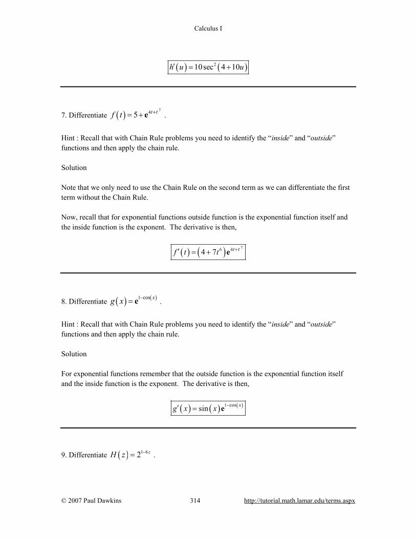
Calculus I
© 2007 Paul Dawkins 314 http://tutorial.math.lamar.edu/terms.aspx
( ) ( )210sec 4 10h u u′ = +
7. Differentiate ( ) 745 t tf t += + e .
Hint : Recall that with Chain Rule problems you need to identify the “inside” and “outside” functions and then apply the chain rule. Solution Note that we only need to use the Chain Rule on the second term as we can differentiate the first term without the Chain Rule. Now, recall that for exponential functions outside function is the exponential function itself and the inside function is the exponent. The derivative is then,
( ) ( ) 76 44 7 t tf t t +′ = + e
8. Differentiate ( ) ( )1 cos xg x −= e .
Hint : Recall that with Chain Rule problems you need to identify the “inside” and “outside” functions and then apply the chain rule. Solution For exponential functions remember that the outside function is the exponential function itself and the inside function is the exponent. The derivative is then,
( ) ( ) ( )1 cossin xg x x −′ = e 9. Differentiate ( ) 1 62 zH z −= .

Calculus I
© 2007 Paul Dawkins 315 http://tutorial.math.lamar.edu/terms.aspx
Hint : Recall that with Chain Rule problems you need to identify the “inside” and “outside” functions and then apply the chain rule. Solution For exponential functions remember that the outside function is the exponential function itself and the inside function is the exponent. The derivative is then,
( ) ( ) ( )1 66 2 ln 2zH z −′ = −
10. Differentiate ( ) ( )1tan 3 1u t t−= − .
Hint : Recall that with Chain Rule problems you need to identify the “inside” and “outside” functions and then apply the chain rule. Solution For this problem the outside function is (hopefully) clearly the inverse tangent and the inside function is the stuff inside of the inverse tangent. The derivative is then,
( )( )2
33 1 1
u tt
′ =− +
11. Differentiate ( ) ( )2 3ln 1 5F y y y= − + .
Hint : Recall that with Chain Rule problems you need to identify the “inside” and “outside” functions and then apply the chain rule. Solution For this problem the outside function is (hopefully) clearly the logarithm and the inside function is the stuff inside of the logarithm. The derivative is then,
( ) ( )2
22 3 2 3
1 10 310 31 5 1 5
y yF y y yy y y y
− += − + =
− + − +

Calculus I
© 2007 Paul Dawkins 316 http://tutorial.math.lamar.edu/terms.aspx
With logarithm problems remember that after differentiating the logarithm (i.e. the outside function) you need to substitute the inside function into the derivative. So, instead of getting just,
1y
we get the following (i.e. we plugged the inside function into the derivative),
2 3
11 5y y− +
Then, we can’t forget of course to multiply by the derivative of the inside function. 12. Differentiate ( ) ( ) ( )( )ln sin cotV x x x= − .
Hint : Recall that with Chain Rule problems you need to identify the “inside” and “outside” functions and then apply the chain rule. Solution For this problem the outside function is (hopefully) clearly the logarithm and the inside function is the stuff inside of the logarithm. The derivative is then,
( ) ( ) ( ) ( ) ( )( ) ( ) ( )( ) ( )
22 cos csc1 cos csc
sin cot sin cotx x
V x x xx x x x
+= + =
− −
With logarithm problems remember that after differentiating the logarithm (i.e. the outside function) you need to substitute the inside function into the derivative. So, instead of getting just,
1x
we get the following (i.e. we plugged the inside function into the derivative),
( ) ( )
1sin cotx x−
Then, we can’t forget of course to multiply by the derivative of the inside function.
13. Differentiate ( ) ( ) ( )6 6sin sinh z z z= + .
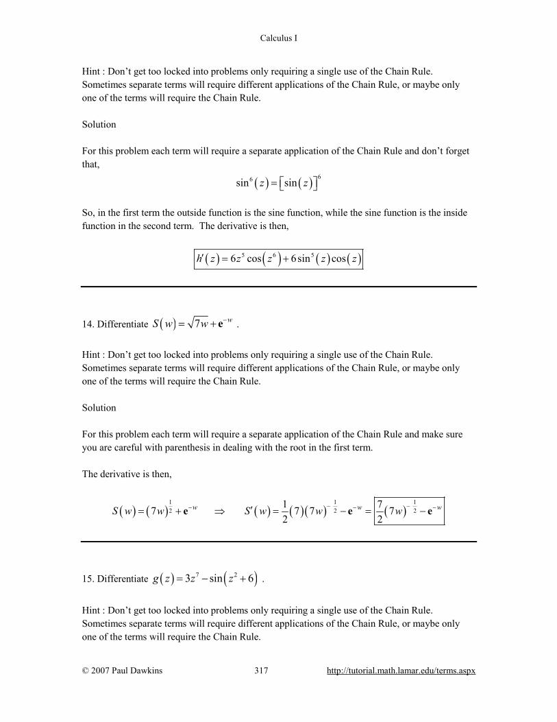
Calculus I
© 2007 Paul Dawkins 317 http://tutorial.math.lamar.edu/terms.aspx
Hint : Don’t get too locked into problems only requiring a single use of the Chain Rule. Sometimes separate terms will require different applications of the Chain Rule, or maybe only one of the terms will require the Chain Rule. Solution For this problem each term will require a separate application of the Chain Rule and don’t forget that,
( ) ( ) 66sin sinz z= So, in the first term the outside function is the sine function, while the sine function is the inside function in the second term. The derivative is then,
( ) ( ) ( ) ( )5 6 56 cos 6sin cosh z z z z z′ = +
14. Differentiate ( ) 7 wS w w −= + e .
Hint : Don’t get too locked into problems only requiring a single use of the Chain Rule. Sometimes separate terms will require different applications of the Chain Rule, or maybe only one of the terms will require the Chain Rule. Solution For this problem each term will require a separate application of the Chain Rule and make sure you are careful with parenthesis in dealing with the root in the first term. The derivative is then,
( ) ( ) ( ) ( ) ( ) ( )1 1 12 2 2
1 77 7 7 72 2
w w wS w w S w w w− −− − −′= + ⇒ = − = −e e e
15. Differentiate ( ) ( )7 23 sin 6g z z z= − + .
Hint : Don’t get too locked into problems only requiring a single use of the Chain Rule. Sometimes separate terms will require different applications of the Chain Rule, or maybe only one of the terms will require the Chain Rule.

Calculus I
© 2007 Paul Dawkins 318 http://tutorial.math.lamar.edu/terms.aspx
Solution For this problem the first term requires no Chain Rule and the second term will require the Chain Rule. The derivative is then,
( ) ( )6 221 2 cos 6g z z z z′ = − +
16. Differentiate ( ) ( )( ) ( )104ln sin 3f x x x x= − − .
Hint : Don’t get too locked into problems only requiring a single use of the Chain Rule. Sometimes separate terms will require different applications of the Chain Rule, or maybe only one of the terms will require the Chain Rule. Solution For this problem each term will require a separate application of the Chain Rule. The derivative is then,
( ) ( )( ) ( )( ) ( ) ( )( )9 93 4 3 4cos
10 4 3 3 cot 10 4 3 3sin
xf x x x x x x x x
x′ = − − − = − − −
17. Differentiate ( ) 6 25h t t t t= − .
Hint : Don’t forget the Product and Quotient Rule. Sometimes, in the process of doing the Product or Quotient Rule you’ll need to use the Chain Rule when differentiating one or both of the terms in the product or quotient. Solution For this problem we’ll need to do the Product Rule to start off the derivative. In the process we’ll need to use the Chain Rule when we differentiate the second term. The derivative is then,
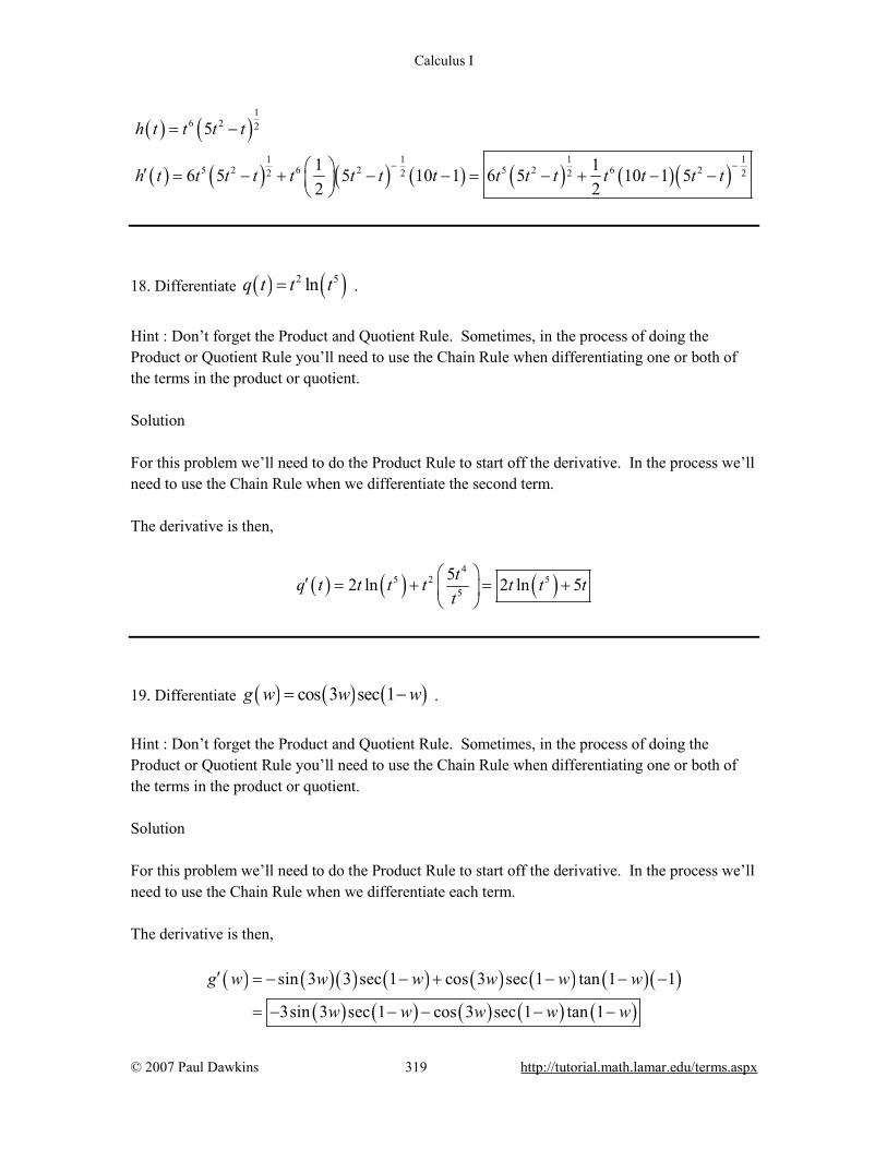
Calculus I
© 2007 Paul Dawkins 319 http://tutorial.math.lamar.edu/terms.aspx
( ) ( )
( ) ( ) ( ) ( ) ( ) ( )( )
16 2 2
1 1 1 15 2 6 2 5 2 6 22 2 2 2
5
1 16 5 5 10 1 6 5 10 1 52 2
h t t t t
h t t t t t t t t t t t t t t t− −
= −
′ = − + − − = − + − −
18. Differentiate ( ) ( )2 5lnq t t t= .
Hint : Don’t forget the Product and Quotient Rule. Sometimes, in the process of doing the Product or Quotient Rule you’ll need to use the Chain Rule when differentiating one or both of the terms in the product or quotient. Solution For this problem we’ll need to do the Product Rule to start off the derivative. In the process we’ll need to use the Chain Rule when we differentiate the second term. The derivative is then,
( ) ( ) ( )4
5 2 55
52 ln 2 ln 5tq t t t t t t tt
′ = + = +
19. Differentiate ( ) ( ) ( )cos 3 sec 1g w w w= − .
Hint : Don’t forget the Product and Quotient Rule. Sometimes, in the process of doing the Product or Quotient Rule you’ll need to use the Chain Rule when differentiating one or both of the terms in the product or quotient. Solution For this problem we’ll need to do the Product Rule to start off the derivative. In the process we’ll need to use the Chain Rule when we differentiate each term. The derivative is then,
( ) ( ) ( ) ( ) ( ) ( ) ( )( )
( ) ( ) ( ) ( ) ( )sin 3 3 sec 1 cos 3 sec 1 tan 1 1
3sin 3 sec 1 cos 3 sec 1 tan 1
g w w w w w w
w w w w w
′ = − − + − − −
= − − − − −
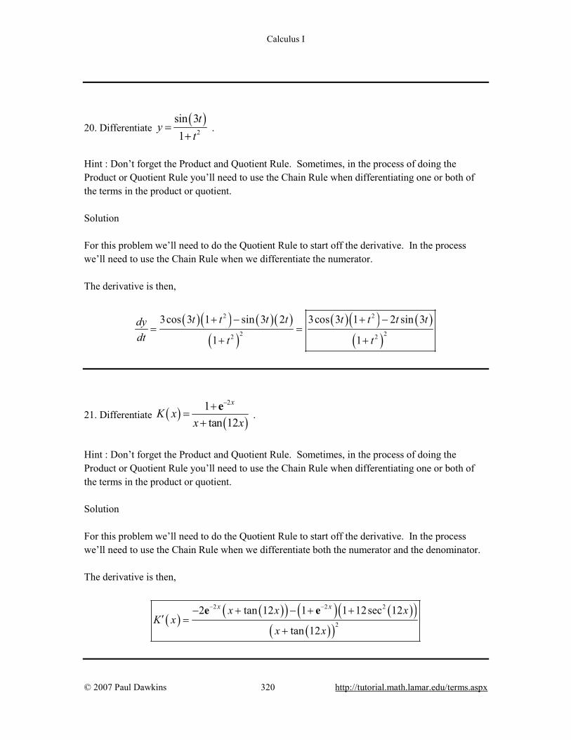
Calculus I
© 2007 Paul Dawkins 320 http://tutorial.math.lamar.edu/terms.aspx
20. Differentiate ( )
2
sin 31
ty
t=
+ .
Hint : Don’t forget the Product and Quotient Rule. Sometimes, in the process of doing the Product or Quotient Rule you’ll need to use the Chain Rule when differentiating one or both of the terms in the product or quotient. Solution For this problem we’ll need to do the Quotient Rule to start off the derivative. In the process we’ll need to use the Chain Rule when we differentiate the numerator. The derivative is then,
( )( ) ( )( )
( )( )( ) ( )
( )
2 2
2 22 2
3cos 3 1 sin 3 2 3cos 3 1 2 sin 3
1 1
t t t t t t t tdydt t t
+ − + −= =
+ +
21. Differentiate ( ) ( )21
tan 12
xK x
x x
−+=
+e
.
Hint : Don’t forget the Product and Quotient Rule. Sometimes, in the process of doing the Product or Quotient Rule you’ll need to use the Chain Rule when differentiating one or both of the terms in the product or quotient. Solution For this problem we’ll need to do the Quotient Rule to start off the derivative. In the process we’ll need to use the Chain Rule when we differentiate both the numerator and the denominator. The derivative is then,
( )( )( ) ( ) ( )( )
( )( )
2 2 2
2
2 tan 12 1 1 12sec 12
tan 12
x xx x xK x
x x
− −− + − + +′ =
+
e e
Calculus I
© 2007 Paul Dawkins 321 http://tutorial.math.lamar.edu/terms.aspx
22. Differentiate ( ) ( )2cos xf x x= e .
Hint : Don’t forget the Product and Quotient Rule. Sometimes, in the process of using the Chain Rule, you’ll also need the Product and/or Quotient Rule. Solution For this problem we’ll start off using the Chain Rule, however when we differentiate the inside function we’ll need to do the Product Rule. The derivative is then,
( ) ( ) ( )2 22 sinx x xf x x x x′ = − +e e e
23. Differentiate ( )5 tan 4z x x= + .
Hint : Sometimes the Chain Rule will need to be done multiple times before we finish taking the derivative. Step 1 This problem will require multiple uses of the Chain Rule and so we’ll step though the derivative process to make each use clear. Here is the first step of the derivative and we’ll need to use the Chain Rule in this step.
( )( )
( )( ) ( )( )
12
12
5 tan 4
1 5 tan 4 5 tan 42
z x x
dz dx x x xdx dx
−
= +
= + +
Step 2 In this step we can see that we’ll need to use the Chain Rule on the second term. The derivative is then,
Calculus I
© 2007 Paul Dawkins 322 http://tutorial.math.lamar.edu/terms.aspx
( )( ) ( )( )1
221 5 tan 4 5 4sec 42
dz x x xdx
−= + +
In this step we were using the Chain Rule on the second term and so when multiplying by the derivative of the inside function we only multiply the second term by the derivative of the inside function and not both terms.
24. Differentiate ( ) ( )( )36 sin 2tf t t−= + −e .
Hint : Sometimes the Chain Rule will need to be done multiple times before we finish taking the derivative. Step 1 This problem will require multiple uses of the Chain Rule and so we’ll step though the derivative process to make each use clear. Here is the first step of the derivative and we’ll need to use the Chain Rule in this step.
( ) ( )( ) ( )( )26 63 sin 2 sin 2t tdf t t tdt
− −′ = + − + −e e
Step 2 In this step we can see that we’ll need to use the Chain Rule on each of the terms. The derivative is then,
( ) ( )( ) ( )( )26 63 sin 2 6 cos 2t tf t t t− −′ = + − − − −e e
25. Differentiate ( ) ( ) ( )( )102 1ln 1 tan 6g x x x−= + − .
Hint : Sometimes the Chain Rule will need to be done multiple times before we finish taking the derivative.
Calculus I
© 2007 Paul Dawkins 323 http://tutorial.math.lamar.edu/terms.aspx
Step 1 This problem will require multiple uses of the Chain Rule and so we’ll step though the derivative process to make each use clear. Here is the first step of the derivative and we’ll need to use the Chain Rule in this step.
( ) ( ) ( )( ) ( ) ( )( )92 1 2 110 ln 1 tan 6 ln 1 tan 6dg x x x x xdx
− −′ = + − + −
Step 2 In this step we can see that we’ll need to use the Chain Rule on each of the terms. The derivative is then,
( ) ( ) ( )( )92 12 2
2 610 ln 1 tan 61 36 1
xg x x xx x
− ′ = + − − + +
26. Differentiate ( ) ( )4 2tan 1h z z= + .
Hint : Sometimes the Chain Rule will need to be done multiple times before we finish taking the derivative. Step 1 This problem will require multiple uses of the Chain Rule and so we’ll step though the derivative process to make each use clear. Also, recall that,
( ) ( ) 44tan tanx x=
Here is the first step of the derivative and we’ll need to use the Chain Rule in this step.
( ) ( ) ( )3 2 24 tan 1 tan 1dh z z zdz
′ = + + Step 2

Calculus I
© 2007 Paul Dawkins 324 http://tutorial.math.lamar.edu/terms.aspx
As we can see the derivative from the previous step will also require the Chain Rule. The derivative is then,
( ) ( ) ( ) ( ) ( ) ( )3 2 2 2 3 2 2 24 tan 1 sec 1 2 8 tan 1 sec 1h z z z z z z z′ = + + = + +
27. Differentiate ( ) ( )( ) 123 12 sin 3f x x x
−= + .
Hint : Sometimes the Chain Rule will need to be done multiple times before we finish taking the derivative. Step 1 This problem will require multiple uses of the Chain Rule and so we’ll step though the derivative process to make each use clear. Here is the first step of the derivative and we’ll need to use the Chain Rule in this step.
( ) ( )( ) ( ) ( )12
2 23 312 sin 3 12 sin 3df x x x x xdx
− ′ = − + +
Step 2 As we can see the derivative from the previous step will also require the Chain Rule on each of the terms. The derivative from this step is,
( ) ( )( ) ( ) ( ) ( ) ( )( )22
23 3112 sin 3 12 12 2sin 3 sin 33
df x x x x x xdx
− − ′ = − + +
Step 3 The second term will again use the Chain Rule as we can see. The derivative is then,
( ) ( )( ) ( ) ( ) ( )22
23 312 sin 3 4 12 6sin 3 cos 3f x x x x x x− − ′ = − + +

Calculus I
© 2007 Paul Dawkins 325 http://tutorial.math.lamar.edu/terms.aspx
28. Find the tangent line to ( ) 24 2 6 xf x x −= − e at 2x = .
Solution Step 1 We know that the derivative of the function will give us the slope of the tangent line so we’ll need the derivative of the function. Differentiating each term will require the Chain Rule as well.
( ) ( )
( ) ( ) ( ) ( ) ( )
122
1 12 2 22 2
4 2 6
1 44 2 2 6 1 4 2 6 62 2
x
x x x
f x x
f x x xx
−
− −− − −
= −
′ = − − = + = +
e
e e e
Step 2 Now all we need to do is evaluate the function and the derivative at the point in question.
( ) ( ) ( )0 042 4 2 6 2 2 6 82
f f ′= − = = + =e e
Step 3 Now all that we need to do is write down the equation of the tangent line.
( ) ( ) ( ) ( )2 2 2 2 8 2 8 14y f f x x y x′= + − = + − → = −
29. Determine where ( ) ( )34 2 8V z z z= − is increasing and decreasing.
Solution Step 1 We’ll first need the derivative because we know that the derivative will give us the rate of change of the function. Here is the derivative.
( ) ( ) ( ) ( ) ( )
( ) ( ) ( ) ( )
3 23 4
2 23 3
4 2 8 3 2 8 2
2 2 8 2 2 8 3 2 2 8 7 16
V z z z z z
z z z z z z z
′ = − + −
= − − + = − −
Note that we factored the derivative to help with the next step. In general we don’t need to do this. Step 2

Calculus I
© 2007 Paul Dawkins 326 http://tutorial.math.lamar.edu/terms.aspx
Next, we need to know where the function is not changing and so all we need to do is set the derivative equal to zero and solve. In this case it’s pretty easy to spot where the derivative will be zero.
( ) ( )23 162 2 8 7 16 0 0, 4, 2.28577
z z z z z z− − = ⇒ = = = =
Step 3 To get the answer to this problem all we need to know is where the derivative is positive (and hence the function is increasing) or negative (and hence the function is decreasing). Because the derivative is continuous we know that the only place it can change sign is where the derivative is zero. So, as we did in this section a quick number line will give us the sign of the derivative for the various intervals. Here is the number line for this problem.
From this we get the following increasing/decreasing information.
16Increasing : 0, 4, 47
16Decreasing : 07
x x x
x
− ∞ < < < < < < ∞
< <
30. The position of an object is given by ( ) ( )sin 3 2 4s t t t= − + . Determine where in the
interval [ ]0,3 the object is moving to the right and moving to the left.
Solution Step 1 We’ll first need the derivative because we know that the derivative will give us the velocity of the object. Here is the derivative.
( ) ( )3cos 3 2s t t′ = −
Calculus I
© 2007 Paul Dawkins 327 http://tutorial.math.lamar.edu/terms.aspx
Step 2 Next, we need to know where the object stops moving and so all we need to do is set the derivative equal to zero and solve.
( ) ( ) 23cos 3 2 0 cos 33
t t− = ⇒ =
A quick calculator computation tells us that,
1 23 cos 0.84113
t − = =
Recalling our work in the Review chapter and a quick check on a unit circle we can see that either 3 0.8411t = − or 3 2 0.8411 5.4421t π= − = can be used for the second angle. Note that either will work, but we’ll use the second simply because it is the positive angle. Putting all of this together and dividing by 3 we can see that the derivative will be zero at,
3 0.8411 2 and 3 5.4421 2 0, 1, 2, 3,
2 20.2804 and 1.8140 0, 1, 2, 3,3 3
t n t n nn nt t n
π ππ π
= + = + = ± ± ±
= + = + = ± ± ±
…
…
Finally, all we need to so is plug in some n’s to determine which solutions fall in the interval we are working on, [ ]0,6 .
0 : 0.2804 1.81401: 2.3748 3.9084
n t tn t t
= = == = =
So, in the interval [ ]0,6 , the object stops moving at the following three points.
0.2804, 1.8140, 2.3748t = Step 3 To get the answer to this problem all we need to know is where the derivative is positive (and hence the object is moving to the right) or negative (and hence the object is moving to the left). Because the derivative is continuous we know that the only place it can change sign is where the derivative is zero. So, as we did in this section a quick number line will give us the sign of the derivative for the various intervals. Here is the number line for this problem.
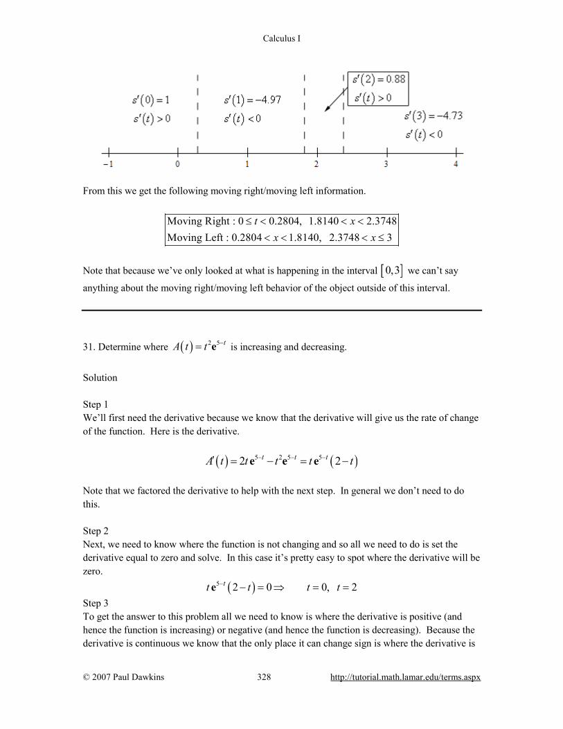
Calculus I
© 2007 Paul Dawkins 328 http://tutorial.math.lamar.edu/terms.aspx
From this we get the following moving right/moving left information.
Moving Right : 0 0.2804, 1.8140 2.3748Moving Left : 0.2804 1.8140, 2.3748 3
t xx x
≤ < < << < < ≤
Note that because we’ve only looked at what is happening in the interval [ ]0,3 we can’t say
anything about the moving right/moving left behavior of the object outside of this interval. 31. Determine where ( ) 2 5 tA t t −= e is increasing and decreasing.
Solution Step 1 We’ll first need the derivative because we know that the derivative will give us the rate of change of the function. Here is the derivative.
( ) ( )5 2 5 52 2t t tA t t t t t− − −′ = − = −e e e Note that we factored the derivative to help with the next step. In general we don’t need to do this. Step 2 Next, we need to know where the function is not changing and so all we need to do is set the derivative equal to zero and solve. In this case it’s pretty easy to spot where the derivative will be zero. ( )5 2 0 0, 2tt t t t− − = ⇒ = =e Step 3 To get the answer to this problem all we need to know is where the derivative is positive (and hence the function is increasing) or negative (and hence the function is decreasing). Because the derivative is continuous we know that the only place it can change sign is where the derivative is
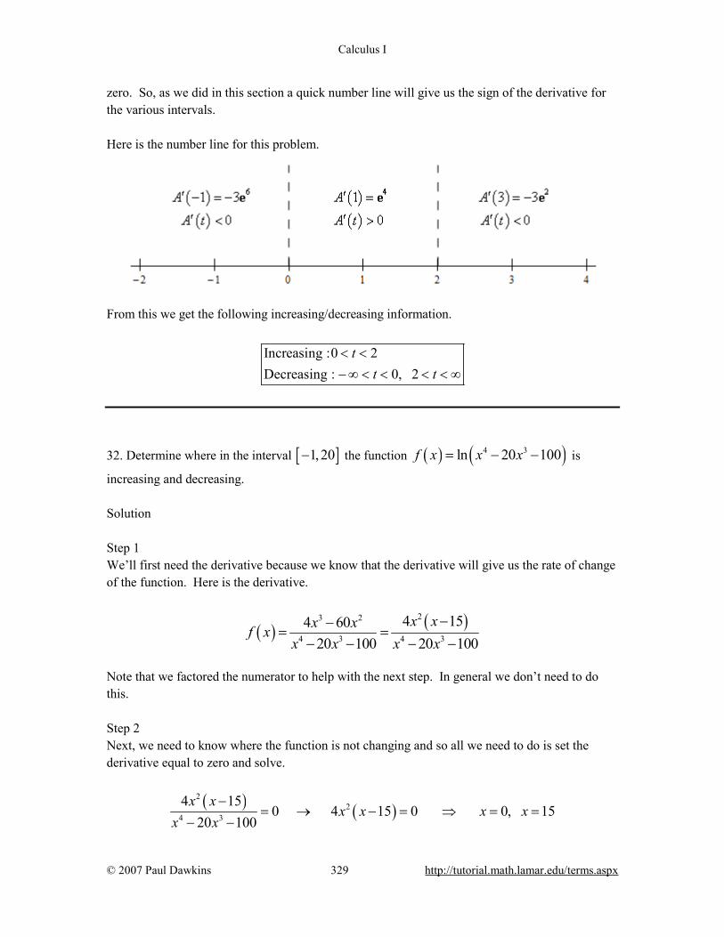
Calculus I
© 2007 Paul Dawkins 329 http://tutorial.math.lamar.edu/terms.aspx
zero. So, as we did in this section a quick number line will give us the sign of the derivative for the various intervals. Here is the number line for this problem.
From this we get the following increasing/decreasing information.
Increasing :0 2Decreasing : 0, 2
tt t
< <− ∞ < < < < ∞
32. Determine where in the interval [ ]1, 20− the function ( ) ( )4 3ln 20 100f x x x= − − is
increasing and decreasing. Solution Step 1 We’ll first need the derivative because we know that the derivative will give us the rate of change of the function. Here is the derivative.
( ) ( )23 2
4 3 4 3
4 154 6020 100 20 100
x xx xf xx x x x
−−= =
− − − −
Note that we factored the numerator to help with the next step. In general we don’t need to do this. Step 2 Next, we need to know where the function is not changing and so all we need to do is set the derivative equal to zero and solve.
( ) ( )
22
4 3
4 150 4 15 0 0, 15
20 100x x
x x x xx x
−= → − = ⇒ = =
− −
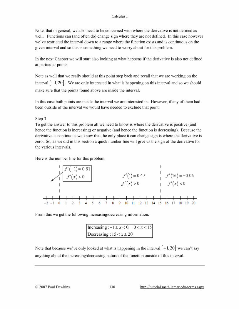
Calculus I
© 2007 Paul Dawkins 330 http://tutorial.math.lamar.edu/terms.aspx
Note, that in general, we also need to be concerned with where the derivative is not defined as well. Functions can (and often do) change sign where they are not defined. In this case however we’ve restricted the interval down to a range where the function exists and is continuous on the given interval and so this is something we need to worry about for this problem. In the next Chapter we will start also looking at what happens if the derivative is also not defined at particular points. Note as well that we really should at this point step back and recall that we are working on the interval [ ]1, 20− . We are only interested in what is happening on this interval and so we should
make sure that the points found above are inside the interval. In this case both points are inside the interval we are interested in. However, if any of them had been outside of the interval we would have needed to exclude that point. Step 3 To get the answer to this problem all we need to know is where the derivative is positive (and hence the function is increasing) or negative (and hence the function is decreasing). Because the derivative is continuous we know that the only place it can change sign is where the derivative is zero. So, as we did in this section a quick number line will give us the sign of the derivative for the various intervals. Here is the number line for this problem.
From this we get the following increasing/decreasing information.
Increasing : 1 0, 0 15Decreasing : 15 20
x xx
− ≤ < < << ≤
Note that because we’ve only looked at what is happening in the interval [ ]1, 20− we can’t say
anything about the increasing/decreasing nature of the function outside of this interval.
Calculus I
© 2007 Paul Dawkins 331 http://tutorial.math.lamar.edu/terms.aspx
Implicit Differentiation
1. For 3 1xy
= do each of the following.
(a) Find y′ by solving the equation for y and differentiating directly. (b) Find y′ by implicit differentiation. (c) Check that the derivatives in (a) and (b) are the same.
(a) Find y′ by solving the equation for y and differentiating directly. Step 1 First we just need to solve the equation for y.
1
3 3y x y x= ⇒ = Step 2 Now differentiate with respect to x.
2
1 33y x
−′ =
(b) Find y′ by implicit differentiation.
Hint : Don’t forget that y is really ( )y x and so we’ll need to use the Chain Rule when taking the
derivative of terms involving y! Also, don’t forget that because y is really ( )y x we may well
have a Product and/or a Quotient Rule buried in the problem. Step 1 First, we just need to take the derivative of everything with respect to x and we’ll need to recall that y is really ( )y x and so we’ll need to use the Chain Rule when taking the derivative of terms
involving y. Also, prior to taking the derivative a little rewrite might make this a little easier. 3 1x y− = Now take the derivative and don’t forget that we actually have a product of functions of x here and so we’ll need to use the Product Rule when differentiating the left side. 3 43 0y x y y− − ′− = Step 2 Finally all we need to do is solve this for y′ .
3
43 3y yyxy x
−
−′ = =
Calculus I
© 2007 Paul Dawkins 332 http://tutorial.math.lamar.edu/terms.aspx
(c) Check that the derivatives in (a) and (b) are the same. Hint : To show they are the same all we need is to plug the formula for y (which we already have….) into the derivative we found in (b) and, potentially with a little work, show that we get the same derivative as we got in (a). From (a) we have a formula for y written explicitly as a function of x so plug that into the derivative we found in (b) and, with a little simplification/work, show that we get the same derivative as we got in (a).
123
1 333 3
y xy xx x
−′ = = =
So, we got the same derivative as we should. 2. For 2 3 4x y+ = do each of the following.
(d) Find y′ by solving the equation for y and differentiating directly. (e) Find y′ by implicit differentiation. (f) Check that the derivatives in (a) and (b) are the same.
(a) Find y′ by solving the equation for y and differentiating directly. Step 1 First we just need to solve the equation for y.
( )1
3 2 2 34 4y x y x= − ⇒ = − Step 2 Now differentiate with respect to x.
( )2
22 33 4y x x
−′ = − −
(b) Find y′ by implicit differentiation.
Hint : Don’t forget that y is really ( )y x and so we’ll need to use the Chain Rule when taking the
derivative of terms involving y! Step 1 First, we just need to take the derivative of everything with respect to x and we’ll need to recall that y is really ( )y x and so we’ll need to use the Chain Rule when taking the derivative of terms
involving y. Taking the derivative gives,

Calculus I
© 2007 Paul Dawkins 333 http://tutorial.math.lamar.edu/terms.aspx
22 3 0x y y′+ = Step 2 Finally all we need to do is solve this for y′ .
2
23
xyy
′ = −
(c) Check that the derivatives in (a) and (b) are the same. Hint : To show they are the same all we need is to plug the formula for y (which we already have….) into the derivative we found in (b) and, potentially with a little work, show that we get the same derivative as we got in (a). From (a) we have a formula for y written explicitly as a function of x so plug that into the derivative we found in (b) and, with a little simplification/work, show that we get the same derivative as we got in (a).
( )
( )2
22 3322
2 3
2 2 43 3 4
x xy x xy x
−′ = − = − = − −
−
So, we got the same derivative as we should. 3. For 2 2 2x y+ = do each of the following.
(g) Find y′ by solving the equation for y and differentiating directly. (h) Find y′ by implicit differentiation. (i) Check that the derivatives in (a) and (b) are the same.
(a) Find y′ by solving the equation for y and differentiating directly. Step 1 First we just need to solve the equation for y.
( )1
2 2 2 22 2y x y x= − ⇒ = ± −
Note that because we have no restriction on y (i.e. we don’t know if y is positive or negative) we really do need to have the “ ± ” there and that does lead to issues when taking the derivative. Hint : Two formulas for y and so two derivatives. Step 2 Now, because there are two formulas for y we will also have two formulas for the derivative, one for each formula for y.
Calculus I
© 2007 Paul Dawkins 334 http://tutorial.math.lamar.edu/terms.aspx
The derivatives are then,
( ) ( ) ( )
( ) ( ) ( )
1 12 22 2
1 12 22 2
2 2 0
2 2 0
y x y x x y
y x y x x y
−
−
′= − ⇒ = − − >
′= − − ⇒ = − <
As noted above the first derivative will hold for 0y > while the second will hold for 0y < and we can use either for 0y = as the plus/minus won’t affect that case. (b) Find y′ by implicit differentiation.
Hint : Don’t forget that y is really ( )y x and so we’ll need to use the Chain Rule when taking the
derivative of terms involving y! Step 1 First, we just need to take the derivative of everything with respect to x and we’ll need to recall that y is really ( )y x and so we’ll need to use the Chain Rule when taking the derivative of terms
involving y. Taking the derivative gives, 2 2 0x y y′+ = Step 2 Finally all we need to do is solve this for y′ .
xyy
′ = −
(c) Check that the derivatives in (a) and (b) are the same. Hint : To show they are the same all we need is to plug the formula for y (which we already have….) into the derivative we found in (b) and, potentially with a little work, show that we get the same derivative as we got in (a). Again, two formulas for y so two derivatives… From (a) we have a formula for y written explicitly as a function of x so plug that into the derivative we found in (b) and, with a little simplification/work, show that we get the same derivative as we got in (a). Also, because we have two formulas for y we will have two formulas for the derivative. First, if 0y > we will have,
( )( )
( )1 1
2 22 21
2 2
2 22
x xy x y x xy x
−′= − ⇒ = − = − = − −
−
Calculus I
© 2007 Paul Dawkins 335 http://tutorial.math.lamar.edu/terms.aspx
Next, if 0y < we will have,
( )( )
( )1 1
2 22 21
2 2
2 22
x xy x y x xy x
−′= − − ⇒ = − = − = −
− −
So, in both cases, we got the same derivative as we should. 4. Find y′ by implicit differentiation for 3 2 62 4y x y x+ − = . Hint : Don’t forget that y is really ( )y x and so we’ll need to use the Chain Rule when taking the
derivative of terms involving y! Step 1 First, we just need to take the derivative of everything with respect to x and we’ll need to recall that y is really ( )y x and so we’ll need to use the Chain Rule when taking the derivative of terms
involving y. Differentiating with respect to x gives, 2 56 8 6y y x y x′ ′+ − = Step 2 Finally all we need to do is solve this for y′ .
( )5
2 52
6 86 1 6 86 1x xy y x x yy
−′ ′− = − ⇒ =−
5. Find y′ by implicit differentiation for ( )2 47 sin 3 12y x y+ = − .
Hint : Don’t forget that y is really ( )y x and so we’ll need to use the Chain Rule when taking the
derivative of terms involving y! Step 1 First, we just need to take the derivative of everything with respect to x and we’ll need to recall that y is really ( )y x and so we’ll need to use the Chain Rule when taking the derivative of terms
involving y. Differentiating with respect to x gives, ( ) 314 3cos 3 4y y x y y′ ′+ = − Step 2 Finally all we need to do is solve this for y′ .
Calculus I
© 2007 Paul Dawkins 336 http://tutorial.math.lamar.edu/terms.aspx
( ) ( ) ( )33
3cos 314 4 3cos 3
14 4x
y y y x yy y
−′ ′+ = − ⇒ =
+
6. Find y′ by implicit differentiation for ( )sinx y x− =e .
Hint : Don’t forget that y is really ( )y x and so we’ll need to use the Chain Rule when taking the
derivative of terms involving y! Step 1 First, we just need to take the derivative of everything with respect to x and we’ll need to recall that y is really ( )y x and so we’ll need to use the Chain Rule when taking the derivative of terms
involving y. Differentiating with respect to x gives, ( )cos 1x y y′+ =e Don’t forget the y′ on the cosine after differentiating. Again, y is really ( )y x and so when
differentiating ( )sin y we really differentiating ( )sin y x and so we are differentiating using
the Chain Rule! Step 2 Finally all we need to do is solve this for y′ .
( ) ( ) ( )1 1 sec
cos
xxy y
y−′ = = −
e e
7. Find y′ by implicit differentiation for 2 7 5 34 2 4x y x x y− = + . Hint : Don’t forget that y is really ( )y x and so we’ll need to use the Chain Rule when taking the
derivative of terms involving y! Also, don’t forget that because y is really ( )y x we may well
have a Product and/or a Quotient Rule buried in the problem. Step 1 First, we just need to take the derivative of everything with respect to x and we’ll need to recall that y is really ( )y x and so we’ll need to use the Chain Rule when taking the derivative of terms
involving y. This also means that the first term on the left side is really a product of functions of x and hence we will need to use the Product Rule when differentiating that term.

Calculus I
© 2007 Paul Dawkins 337 http://tutorial.math.lamar.edu/terms.aspx
Differentiating with respect to x gives, 7 2 6 4 28 28 2 5 12xy x y y x y y′ ′+ − = + Step 2 Finally all we need to do is solve this for y′ .
( )7 4
7 4 2 2 62 2 6
8 5 28 5 2 12 2812 28
xy xxy x y x y y yy x y
− −′ ′− − = − ⇒ =−
8. Find y′ by implicit differentiation for ( ) 22cos 2 1yx y x+ + =e .
Hint : Don’t forget that y is really ( )y x and so we’ll need to use the Chain Rule when taking the
derivative of terms involving y! Also, don’t forget that because y is really ( )y x we may well
have a Product and/or a Quotient Rule buried in the problem. Step 1 First, we just need to take the derivative of everything with respect to x and we’ll need to recall that y is really ( )y x and so we’ll need to use the Chain Rule when taking the derivative of terms
involving y. This also means that the second term on the left side is really a product of functions of x and hence we will need to use the Product Rule when differentiating that term. Differentiating with respect to x gives,
( ) ( ) 2 222 2 sin 2 2 0y yx y x y y y x′ ′− + + + + =e e Step 2 Finally all we need to do is solve this for y′ (with some potentially messy algebra).
( ) ( )( )( ) ( )
( )( )
2 2
2 2
2
2
2 2
2 2
2
2
2 sin 2 2 sin 2 2 0
2 2sin 2 0 2 sin 2
2 sin 2
2 2sin 2
y y
y y
y
y
x x y y x y y y x
yx x y y x x y
x x yy
yx x y
′ ′− + − + + + =
′− + = + + −
+ −′ =
− +
e e
e e
e
e
9. Find y′ by implicit differentiation for ( )2 4 2tan 3x y x y= + .
Hint : Don’t forget that y is really ( )y x and so we’ll need to use the Chain Rule when taking the
derivative of terms involving y! Also, don’t forget that because y is really ( )y x we may well
have a Product and/or a Quotient Rule buried in the problem. Step 1

Calculus I
© 2007 Paul Dawkins 338 http://tutorial.math.lamar.edu/terms.aspx
First, we just need to take the derivative of everything with respect to x and we’ll need to recall that y is really ( )y x and so we’ll need to use the Chain Rule when taking the derivative of terms
involving y. This also means that the when doing Chain Rule on the first tangent on the left side we will need to do Product Rule when differentiating the “inside term”. Differentiating with respect to x gives,
( ) ( )4 2 3 2 2 42 4 sec 3 2x y x y y x y y y′ ′+ = + Step 2 Finally all we need to do is solve this for y′ (with some potentially messy algebra).
( ) ( )( )( ) ( )
( )( )
4 2 2 4 2 3 2 2 4
2 3 2 2 4 4 2 2 4
4 2 2 4
2 3 2 2 4
2 sec 4 sec 3 2
4 sec 2 3 2 sec
3 2 sec
4 sec 2
x y x y x y y x y y y
x y x y y y x y x y
x y x yy
x y x y y
′ ′+ = +
′− = −
−′ =
−
10. Find the equation of then tangent line to 4 2 3x y+ = at ( )1, 2− .
Hint : We know how to compute the slope of tangent lines and with implicit differentiation that shouldn’t be too hard at this point. Step 1 The first thing to do is use implicit differentiation to find y′ for this function.
3
3 24 2 0 xx y y yy
′ ′+ = ⇒ = −
Step 2 Evaluating the derivative at the point in question to get the slope of the tangent line gives,
1, 2
2 22x y
m y= =−
′= = − =−
Step 3 Now, we just need to write down the equation of the tangent line.
( ) ( ) ( ) ( )2 2 1 2 1 2 2 2y x y x x− − = − ⇒ = − − = −
11. Find the equation of then tangent line to 2 2 23xy y x= +e at ( )0,3 .
Calculus I
© 2007 Paul Dawkins 339 http://tutorial.math.lamar.edu/terms.aspx
Hint : We know how to compute the slope of tangent lines and with implicit differentiation that shouldn’t be too hard at this point. Step 1 The first thing to do is use implicit differentiation to find y′ for this function.
2 2
2 2 22
2 22 2 3 22 3
xx x
xx yyy y y x y
y−′ ′ ′+ = + ⇒ =
−ee e
e
Step 2 Evaluating the derivative at the point in question to get the slope of the tangent line gives,
0, 3
18 63x y
m y= =
−′= = = −
Step 3 Now, we just need to write down the equation of the tangent line.
( )3 6 0 6 3y x y x− = − − ⇒ = − + 12. Assume that ( )x x t= , ( )y y t= and ( )z z t= and differentiate 2 3 4 1x y z− + = with
respect to t. Hint : This is just implicit differentiation like we’ve been doing to this point. The only difference is that now all the functions are functions of some fourth variable, t. Outside of that there is nothing different between this and the previous problems. Solution Differentiating with respect to t gives,
2 32 3 4 0x x y y z z′ ′ ′− + =
Note that because we were not asked to give the formula for a specific derivative we don’t need to go any farther. We could however, if asked, solved this for any of the three derivatives that are present.
13. Assume that ( )x x t= , ( )y y t= and ( )z z t= and differentiate ( ) ( )2 3cos sin 4x y y z= +
with respect to t. Hint : This is just implicit differentiation like we’ve been doing to this point. The only difference is that now all the functions are functions of some fourth variable, t. Outside of that there is nothing different between this and the previous problems. Solution
Calculus I
© 2007 Paul Dawkins 340 http://tutorial.math.lamar.edu/terms.aspx
Differentiating with respect to t gives,
( ) ( ) ( ) ( )2 2 32 cos sin 3 4 cos 4x x y x y y y y z y z′ ′ ′ ′− = + +
Note that because we were not asked to give the formula for a specific derivative we don’t need to go any farther. We could however, if asked, solved this for any of the three derivatives that are present.
Related Rates 1. In the following assume that x and y are both functions of t. Given 2x = − , 1y = and 4x′ = − determine y′ for the following equation.
2 2 3 4 46 2 yy x x −+ = − e Hint : This is just like the problems worked in the section notes. The only difference is that you’ve been given the equation and all the needed information and so you won’t have to worry about finding that. Step 1 The first thing that we need to do here is use implicit differentiation to differentiate the equation with respect to t. 2 4 4 3 4 412 2 3 4y yy y x x x x x y− −′ ′ ′ ′+ = − +e e Step 2 All we need to do now is plug in the given information and solve for y′ .
81112 16 48 32y y y′ ′ ′+ = − ⇒ =
2. In the following assume that x, y and z are all functions of t. Given 4x = , 2y = − , 1z = ,
9x′ = and 3y′ = − determine z′ for the following equation.
( ) 3 2 2 21 5 3x y z y z x− + = + − Hint : This is just like the problems worked in the section notes. The only difference is that you’ve been given the equation and all the needed information and so you won’t have to worry about finding that.

Calculus I
© 2007 Paul Dawkins 341 http://tutorial.math.lamar.edu/terms.aspx
Step 1 The first thing that we need to do here is use implicit differentiation to differentiate the equation with respect to t. ( ) 2 2 21 15 2 2 2x y x y z z y y z y z z x x′ ′ ′ ′ ′ ′− − + = + + Step 2 All we need to do now is plug in the given information and solve for z′ .
45727 12 15 12 8 72z z z′ ′ ′+ + = + + ⇒ =
3. For a certain rectangle the length of one side is always three times the length of the other side.
(a) If the shorter side is decreasing at a rate of 2 inches/minute at what rate is the longer side decreasing?
(b) At what rate is the enclosed area decreasing when the shorter side is 6 inches long and is decreasing at a rate of 2 inches/minute?
Hint : The equation needed here is a really simple equation. In fact, so simple it might be easy to miss… (a) If the shorter side is decreasing at a rate of 2 inches/minute at what rate is the longer side decreasing? Step 1 Let’s call the shorter side x and the longer side y. We know that 2x′ = − and want to find y′ . Now all we need is an equation that relates these two quantities and from the problem statement we know the longer side is three times shorter side and so the equation is, 3y x= Step 2 Next step is to simply differentiate the equation with respect to t. 3y x′ ′=
Step 3
Finally, plug in the known quantity and solve for what we want : 6y′ = −
Hint : Once we have the equation for the area we can either simplify the equation as we did in this section or we can use the result from the previous step and the equation directly. (b) At what rate is the enclosed area decreasing when the shorter side is 6 inches long and is decreasing at a rate of 2 inches/minute? Step 1
Calculus I
© 2007 Paul Dawkins 342 http://tutorial.math.lamar.edu/terms.aspx
Again we’ll call the shorter side x and the longer side y as with the last part. We know that 6x = , 2x′ = − and want to find A′ .
The equation we’ll need is just the area formula for a rectangle : A xy= At this point we can either leave the equation as is and differentiate it or we can plug in 3y x= to simplify the equation down to a single variable then differentiate. Doing this gives, ( ) 23A x x= Step 2 Now we need to differentiate with respect to t. If we use the equation in terms of only x, which is probably the easiest to use we get, 6A x x′ ′=
If we use the equation in terms of both x and y we get, A x y x y′ ′ ′= + Step 3 Now all we need to do is plug in the known quantities and solve for A′ . Using the equation in terms of only x is the “easiest” because we already have all the known quantities from the problem statement itself. Doing this gives,
( )( )6 6 2 72A′ = − = − Now let’s use the equation in terms of x and y. We know that 6x = and 2x′ = − from the
problem statement. From part (a) we have 6y′ = − and we also know that ( )3 6 18y = = .
Using these gives,
( ) ( ) ( )( )6 6 2 18 72A′ = − + − = − So, as we can see both gives the same result but the second method is slightly more work, although not much more. 4. A thin sheet of ice is in the form of a circle. If the ice is melting in such a way that the area of the sheet is decreasing at a rate of 0.5 m2/sec at what rate is the radius decreasing when the area of the sheet is 12 m2 ? Step 1 We’ll call the area of the sheet A and the radius r and we know that the area of a circle is given by,
Calculus I
© 2007 Paul Dawkins 343 http://tutorial.math.lamar.edu/terms.aspx
2A rπ= We know that 0.5A′ = − and want to determine r′ when 12A = . Step 2 Next step is to simply differentiate the equation with respect to t. 2A r rπ′ ′=
Step 3 Now, to finish this problem off we’ll first need to go back to the equation of the area and use the fact that we know the area at the point we are interested in and determine the radius at that time.
2 1212 1.9544r rππ
= ⇒ = =
The rate of change of the radius is then,
( )0.5 2 1.9544 0.040717r rπ ′ ′− = ⇒ = − 5. A person is standing 350 feet away from a model rocket that is fired straight up into the air at a rate of 15 ft/sec. At what rate is the distance between the person and the rocket increasing (a) 20 seconds after liftoff? (b) 1 minute after liftoff? Step 1 Here is a sketch for this situation that will work for both parts so we’ll put it here.
Step 2 In both parts we know that 15y′ = and want to determine z′ for each given time. Using the Pythagorean Theorem we get the following equation to relate y and z. 2 2 2 2350 122500z y y= + = +

Calculus I
© 2007 Paul Dawkins 344 http://tutorial.math.lamar.edu/terms.aspx
Step 3 Finally, let’s differentiate this with respect to t and we can even solve it for z′ so the actual solution will be quick and simple to find.
2 2 y yz z y y zz
′′ ′ ′= ⇒ =
We have now reached a point where the process will differ for each part. (a) At what rate is the distance between the person and the rocket increasing 20 seconds after liftoff? To finish off this problem all we need to do is determine y (from the speed of the rocket and given time) and z (reusing the Pythagorean Theorem).
( )( ) 2 215 20 300 300 350 212500 50 85 460.9772y z= = = + = = =
The rate of change of the distance between the two is then,
( )( )300 159.76187
460.9772z′ = =
(b) At what rate is the distance between the person and the rocket increasing 1 minute after liftoff? This part is nearly identical to the first part with the exception that the time is now 60 seconds (and note that we MUST be in seconds because the speeds are in time of seconds). Here is the work for this problem.
( ) ( )
( ) ( )
2 215 60 900 900 350 932500 50 373 965.6604
900 1513.98007
965.6604
y z
z
= = = + = = =
′ = =
6. A plane is 750 meters in the air flying parallel to the ground at a speed of 100 m/s and is initially 2.5 kilometers away from a radar station. At what rate is the distance between the plane and the radar station changing (a) initially and (b) 30 seconds after it passes over the radar station? See the (probably bad) sketch below to help visualize the problem.

Calculus I
© 2007 Paul Dawkins 345 http://tutorial.math.lamar.edu/terms.aspx
(a) At what rate is the distance between the plane and the radar station changing initially? Step 1 For this part we know that 100x′ = − when 2500x = . In this case note that x′ must be negative because x will be decreasing in this part. Also note that we converted x to meters since all the other quantities are in meters. Here is a sketch for this part.
Step 2 We want to determine z′ in this part so using the Pythagorean Theorem we get the following equation to relate x and z. 2 2 2 2750 562500z x x= + = + Step 3 Finally, let’s differentiate this with respect to t and we can even solve it for z′ so the actual solution will be quick and simple to find.
2 2 x xz z x x zz
′′ ′ ′= ⇒ =
Step 4 To finish off this problem all we need to do is determine z (reusing the Pythagorean Theorem) and then plug into the equation from Step 3 above.
2 22500 750 6812500 250 109 2610.0766z = + = = =
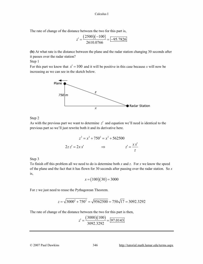
Calculus I
© 2007 Paul Dawkins 346 http://tutorial.math.lamar.edu/terms.aspx
The rate of change of the distance between the two for this part is,
( )( )2500 10095.7826
2610.0766z
−′ = = −
(b) At what rate is the distance between the plane and the radar station changing 30 seconds after it passes over the radar station? Step 1 For this part we know that 100x′ = and it will be positive in this case because x will now be increasing as we can see in the sketch below.
Step 2 As with the previous part we want to determine z′ and equation we’ll need is identical to the previous part so we’ll just rewrite both it and its derivative here.
2 2 2 2750 562500
2 2
z x xx xz z x x zz
= + = +′
′ ′ ′= ⇒ =
Step 3 To finish off this problem all we need to do is determine both x and z. For x we know the speed of the plane and the fact that it has flown for 30 seconds after passing over the radar station. So x is, ( )( )100 30 3000x = = For z we just need to reuse the Pythagorean Theorem.
2 23000 750 9562500 750 17 3092.3292z = + = = = The rate of change of the distance between the two for this part is then,
( ) ( )3000 10097.0143
3092.3292z′ = =

Calculus I
© 2007 Paul Dawkins 347 http://tutorial.math.lamar.edu/terms.aspx
7. Two people are at an elevator. At the same time one person starts to walk away from the elevator at a rate of 2 ft/sec and the other person starts going up in the elevator at a rate of 7 ft/sec. What rate is the distance between the two people changing 15 seconds later? Step 1 Here is a sketch for this part.
We want to determine z′ after 15 seconds given that 2x′ = , 7y′ = and assuming that they start at the same point. Step 2 Hopefully it’s clear that we’ll need the Pythagorean Theorem to solve this problem so here is that. 2 2 2z x y= + Step 3 Finally, let’s differentiate this with respect to t and we can even solve it for z′ so the actual solution will be quick and simple to find.
2 2 2 x x y yz z x x y y zz
′ ′+′ ′ ′ ′= + ⇒ =
Step 4 To finish off this problem all we need to do is determine all three lengths of the triangle in the sketch above. We can find x and y using their speeds and time while we can find z by reusing the Pythagorean Theorem.
( )( ) ( )( )2 2
2 15 30 7 15 105
30 105 11925 15 53 109.2016
x y
z
= = = =
= + = = =
The rate of change of the distance between the two people is then,
( )( ) ( )( )30 2 105 77.2801
109.2016z
+′ = =

Calculus I
© 2007 Paul Dawkins 348 http://tutorial.math.lamar.edu/terms.aspx
8. Two people on bikes are at the same place. One of the bikers starts riding directly north at a rate of 8 m/sec. Five seconds after the first biker started riding north the second starts to ride directly east at a rate of 5 m/sec. At what rate is the distance between the two riders increasing 20 seconds after the second person started riding? Step 1 Here is a sketch of this situation.
We want to determine z′ after 20 seconds after the second biker starts riding east given that
5x′ = , 8y′ = and assuming that they start at the same point. Step 2 Hopefully it’s clear that we’ll need the Pythagorean Theorem to solve this problem so here is that. 2 2 2z x y= + Step 3 Finally, let’s differentiate this with respect to t and we can even solve it for z′ so the actual solution will be quick and simple to find.
2 2 2 x x y yz z x x y y zz
′ ′+′ ′ ′ ′= + ⇒ =
Step 4 To finish off this problem all we need to do is determine all three lengths of the triangle in the sketch above. We can find x and y using their speeds and time while we can find z by reusing the Pythagorean Theorem. Note that the biker riding east will be riding for 20 seconds and the biker riding north will be riding for 25 seconds (this biker started 5 seconds earlier…).
( ) ( ) ( )( )2 2
5 20 100 8 25 200
100 200 50000 100 5 223.6068
x y
z
= = = =
= + = = =
The rate of change of the distance between the two people is then,
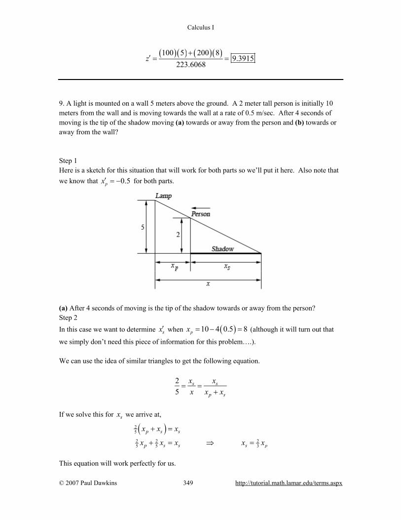
Calculus I
© 2007 Paul Dawkins 349 http://tutorial.math.lamar.edu/terms.aspx
( ) ( ) ( )( )100 5 200 89.3915
223.6068z
+′ = =
9. A light is mounted on a wall 5 meters above the ground. A 2 meter tall person is initially 10 meters from the wall and is moving towards the wall at a rate of 0.5 m/sec. After 4 seconds of moving is the tip of the shadow moving (a) towards or away from the person and (b) towards or away from the wall? Step 1 Here is a sketch for this situation that will work for both parts so we’ll put it here. Also note that we know that 0.5px′ = − for both parts.
(a) After 4 seconds of moving is the tip of the shadow towards or away from the person? Step 2 In this case we want to determine sx′ when ( )10 4 0.5 8px = − = (although it will turn out that
we simply don’t need this piece of information for this problem….). We can use the idea of similar triangles to get the following equation.
25
s s
p s
x xx x x
= =+
If we solve this for sx we arrive at,
( )2
5
2 2 25 5 3 p
p s s
p s s s
x x x
x x x x x
+ =
+ = ⇒ =
This equation will work perfectly for us.
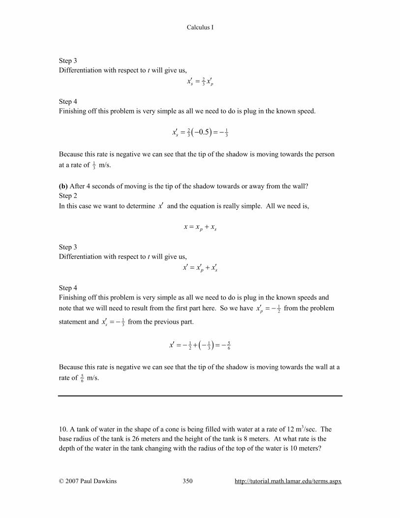
Calculus I
© 2007 Paul Dawkins 350 http://tutorial.math.lamar.edu/terms.aspx
Step 3 Differentiation with respect to t will give us, 2
3 psx x′ ′= Step 4 Finishing off this problem is very simple as all we need to do is plug in the known speed.
( )2 13 30.5sx′ = − = −
Because this rate is negative we can see that the tip of the shadow is moving towards the person at a rate of 1
3 m/s. (b) After 4 seconds of moving is the tip of the shadow towards or away from the wall? Step 2 In this case we want to determine x′ and the equation is really simple. All we need is, p sx x x= + Step 3 Differentiation with respect to t will give us, p sx x x′ ′ ′= + Step 4 Finishing off this problem is very simple as all we need to do is plug in the known speeds and note that we will need to result from the first part here. So we have 1
2px′ = − from the problem
statement and 13sx′ = − from the previous part.
( ) 51 12 3 6x′ = − + − = −
Because this rate is negative we can see that the tip of the shadow is moving towards the wall at a rate of 5
6 m/s. 10. A tank of water in the shape of a cone is being filled with water at a rate of 12 m3/sec. The base radius of the tank is 26 meters and the height of the tank is 8 meters. At what rate is the depth of the water in the tank changing with the radius of the top of the water is 10 meters?
Calculus I
© 2007 Paul Dawkins 351 http://tutorial.math.lamar.edu/terms.aspx
Step 1 Here is a sketch of the cross section of the tank and it is not even remotely to scale as I found it easier to reuse an old image that I had lying around. I can be a little lazy sometimes….
We want to determine h′ when 10r = and we know that 12V ′ = . Step 2 We’ll need the equation for the volume of a cone. 21
3V r hπ= This is a problem however as it has both r and h in it and it would be best to have only h since we need h′ . We can use similar triangles to fix this up. Based on similar triangles we get the following equation which can be solved for r.
134
268
r r hh
= ⇒ =
Plugging this into the volume equation gives, 3169
48V hπ= Step 3 Next, let’s differentiate this with respect to t. 2169
16V h hπ′ ′= Step 4 To finish off this problem all we need to do is determine the value of h for the time we are interested in. This can easily be done from the similar triangle equation and the fact that we know 10r = .
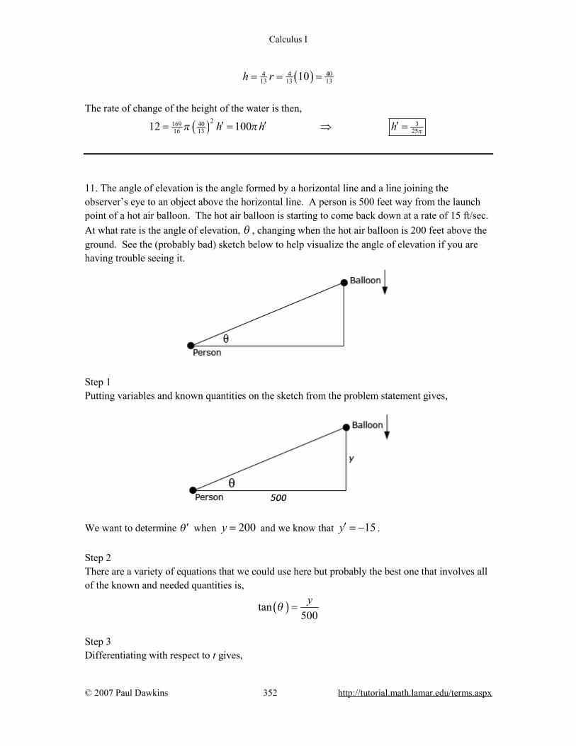
Calculus I
© 2007 Paul Dawkins 352 http://tutorial.math.lamar.edu/terms.aspx
( ) 404 413 13 1310h r= = =
The rate of change of the height of the water is then,
( )2169 40 316 13 2512 100h h h ππ π′ ′ ′= = ⇒ =
11. The angle of elevation is the angle formed by a horizontal line and a line joining the observer’s eye to an object above the horizontal line. A person is 500 feet way from the launch point of a hot air balloon. The hot air balloon is starting to come back down at a rate of 15 ft/sec. At what rate is the angle of elevation, θ , changing when the hot air balloon is 200 feet above the ground. See the (probably bad) sketch below to help visualize the angle of elevation if you are having trouble seeing it.
Step 1 Putting variables and known quantities on the sketch from the problem statement gives,
We want to determine θ ′ when 200y = and we know that 15y′ = − . Step 2 There are a variety of equations that we could use here but probably the best one that involves all of the known and needed quantities is,
( )tan500
yθ =
Step 3 Differentiating with respect to t gives,
Calculus I
© 2007 Paul Dawkins 353 http://tutorial.math.lamar.edu/terms.aspx
( ) ( )2 2sec cos500 500y y
θ θ θ θ′ ′
′ ′= ⇒ =
Step 4 To finish off this problem all we need to do is determine the value of θ for the time in question. We can either use the original equation to do this or we could acknowledge that all we really need is ( )cos θ and we could do a little right triangle trig to determine that.
For this problem we’ll just use the original equation to find the value of θ .
( ) ( )1200 2500 5tan tan 0.38051radiansθ θ −= ⇒ = =
The rate of change of the angle of elevation is then,
( )215 cos 0.38051 0.2586500
θ−′ = = −
Higher Order Derivatives 1. Determine the fourth derivative of ( ) 7 4 33 6 8 12 18h t t t t t= − + − +
Step 1 Not much to this problem other than to take four derivatives so each step will show each successive derivatives until we get to the fourth. The first derivative is then, ( ) 6 3 221 24 24 12h t t t t′ = − + − Step 2 The second derivative is, ( ) 5 2126 72 48h t t t t′′ = − +
Step 3 The third derivative is, ( ) 4630 144 48h t t t′′′ = − + Step 4 The fourth, and final derivative for this problem, is,
( ) ( )4 32520 144h t t= −
Calculus I
© 2007 Paul Dawkins 354 http://tutorial.math.lamar.edu/terms.aspx
2. Determine the fourth derivative of ( ) 3 2 1V x x x x= − + −
Step 1 Not much to this problem other than to take four derivatives so each step will show each successive derivatives until we get to the fourth. The first derivative is then, ( ) 23 2 1V x x x′ = − + Step 2 The second derivative is, ( ) 6 2V x x′′ = −
Step 3 The third derivative is, ( ) 6V x′′′ = Step 4 The fourth, and final derivative for this problem, is,
( ) ( )4 0V x = Note that we could have just as easily used the Fact from the notes to arrive at this answer in one step.
3. Determine the fourth derivative of ( ) 5 32
148
f x x xx
= − −
Step 1 Not much to this problem other than to take four derivatives so each step will show each successive derivatives until we get to the fourth. After a quick rewrite of the function to help with the differentiation the first derivative is,
( ) ( )3 21 1
2 35 52 21 12 1 148 5 4 2
f x x x x f x x x x− −− −′= − − ⇒ = + −
Step 2 The second derivative is,

Calculus I
© 2007 Paul Dawkins 355 http://tutorial.math.lamar.edu/terms.aspx
( )7 3
45 224 3 125 4 4
f x x x x− −−′′ = − − +
Step 3 The third derivative is,
( )12 5
55 2168 33125 8
f x x x x− −−′′′ = + −
Step 4 The fourth, and final derivative for this problem, is,
( ) ( )17 7
4 65 22016 1515625 16
f x x x x− −−= − − +
4. Determine the fourth derivative of ( ) ( ) ( )37sin cos 1 2wf w w= + −
Step 1 Not much to this problem other than to take four derivatives so each step will show each successive derivatives until we get to the fourth. The first derivative is then,
( ) ( ) ( )37 cos 2sin 1 23
wf w w′ = + −
Step 2 The second derivative is,
( ) ( ) ( )37 sin 4 cos 1 29
wf w w′′ = − − −
Step 3 The third derivative is,
( ) ( ) ( )37 cos 8sin 1 227
wf w w′′′ = − − −
Step 4 The fourth, and final derivative for this problem, is,
( ) ( ) ( ) ( )43
7 sin 16cos 1 281
wf w w= + −
Calculus I
© 2007 Paul Dawkins 356 http://tutorial.math.lamar.edu/terms.aspx
5. Determine the fourth derivative of ( )5 48ln 2zy z−= +e
Step 1 Not much to this problem other than to take four derivatives so each step will show each successive derivatives until we get to the fourth. The first derivative is then,
3
5 5 14
85 8 5 322
z zdy z zdx z
− − − = − + = − +
e e
Step 2 The second derivative is,
2
5 22 25 32zd y z
dx− −= −e
Step 3 The third derivative is,
3
5 33 125 64zd y z
dx− −= − +e
Step 4 The fourth, and final derivative for this problem, is,
4
5 44 625 192zd y z
dx− −= −e
6. Determine the second derivative of ( ) ( )3sin 2 9g x x x= −
Step 1 Not much to this problem other than to take two derivatives so each step will show each successive derivatives until we get to the second. The first derivative is then,
( ) ( ) ( )2 36 9 cos 2 9g x x x x′ = − − Step 2 Do not forget that often we will end up needing to do a product rule in the second derivative even though we did not need to do that in the first derivative. The second derivative is then,
( ) ( ) ( ) ( )23 2 312 cos 2 9 6 9 sin 2 9g x x x x x x x′′ = − − − −

Calculus I
© 2007 Paul Dawkins 357 http://tutorial.math.lamar.edu/terms.aspx
7. Determine the second derivative of ( )3ln 7z x= −
Step 1 Not much to this problem other than to take two derivatives so each step will show each successive derivatives until we get to the second. The first derivative is then,
2
3
37
dz xdx x
−=
−
Step 2 Do not forget that often we will end up needing to do a quotient rule in the second derivative even though we did not need to do that in the first derivative. The second derivative is then,
( ) ( )( )
( ) ( )
3 2 22 4
2 22 3 3
6 7 3 3 42 3
7 7
x x x xd z x xdx x x
− − − − − − −= =
− −
8. Determine the second derivative of ( )( )42
2
6 2Q v
v v=
+ −
Step 1 Not much to this problem other than to take two derivatives so each step will show each successive derivatives until we get to the second. We’ll do a quick rewrite of the function to help with the derivatives and then the first derivative is,
( ) ( )( ) ( )( )
42
52
2 6 2
8 2 2 6 2
Q v v v
Q v v v v
−
−
= + −
′ = − − + −
Step 2 Do not forget that often we will end up needing to do a product rule in the second derivative even though we did not need to do that in the first derivative. The second derivative is then,
( ) ( ) ( ) ( )5 622 216 6 2 40 2 2 6 2Q v v v v v v− −
′′ = + − + − + − 9. Determine the second derivative of ( ) ( )2cos 7H t t=
Step 1 Not much to this problem other than to take two derivatives so each step will show each successive derivatives until we get to the second. The first derivative is then,
Calculus I
© 2007 Paul Dawkins 358 http://tutorial.math.lamar.edu/terms.aspx
( ) ( ) ( )14cos 7 sin 7H t t t′ = − Step 2 Do not forget that often we will end up needing to do a product rule in the second derivative even though we did not need to do that in the first derivative. The second derivative is then,
( ) ( ) ( ) ( ) ( ) ( ) ( )2 298sin 7 sin 7 98cos 7 cos 7 98sin 7 98cos 7H t t t t t t t′′ = − = − Note that, in this case, if we recall our trig formulas we could have reduced the product in the first derivative to a single trig function which would have then allowed us to avoid the product rule for the second derivative. Can you figure out what the formula is? 10. Determine the second derivative of 3 22 1 4x y y+ = − Step 1 Not much to this problem other than to take two derivatives so each step will show each successive derivatives until we get to the second. Note however that we are going to have to do implicit differentiation to do each derivative. Here is the work for the first derivative. If you need a refresher on implicit differentiation go back to that section and check some of the problems in that section.
( )
2
2 22
6 2 46 32 4 6
2 4 2
x y y yx xy y x y
y y
′ ′+ = −
− −′ ′+ = − ⇒ = =+ +
Step 2 Now, the second derivative will also need implicit differentiation. Note as well that we can work with the first derivative in its present form which will require the quotient rule or we can rewrite it as,
( ) 123 2y x y −′ = − + and use the product rule. These get messy enough as it is so we’ll go with the product rule to try and keep the “mess” down a little. Using implicit differentiation to take the derivative of first derivative gives,
( ) ( ) ( )1 226 2 3 2dy y x y x y ydx
− −′′ ′ ′= = − + + + Step 3 Finally, recall that we don’t want a y′ in the second derivative so to finish this out we need to plug in the formula for y′ (which we know…) and do a little simplifying to get the final answer.
Calculus I
© 2007 Paul Dawkins 359 http://tutorial.math.lamar.edu/terms.aspx
( ) ( ) ( )( ) ( ) ( )1 2 1 1 32 2 46 2 3 2 3 2 6 2 9 2y x y x y x y x y x y− − − − −′′ = − + + + − + = − + − +
11. Determine the second derivative of 26 1y xy− = Step 1 Not much to this problem other than to take two derivatives so each step will show each successive derivatives until we get to the second. Note however that we are going to have to do implicit differentiation to do each derivative. Here is the work for the first derivative. If you need a refresher on implicit differentiation go back to that section and check some of the problems in that section.
( )
2
22
6 2 0
6 26 2
y y xy yyxy y y y
xy
′ ′− − =
′ ′− = ⇒ =−
Step 2 Now, the second derivative will also need implicit differentiation. Note as well that we can work with the first derivative in its present form which will require the quotient rule or we can rewrite it as,
( ) 12 6 2y y xy −′ = − and use the product rule. These get messy enough as it is so we’ll go with the product rule to try and keep the “mess” down a little. Using implicit differentiation to take the derivative of first derivative gives,
( ) ( ) ( ) ( )1 222 6 2 6 2 2 2dy y y y xy y xy y xydx
− −′′ ′ ′ ′= = − − − − − Step 3 Finally, recall that we don’t want a y′ in the second derivative. So, to finish this out let’s do a little “simplifying” of the to make it “easier” to plug in the formula for y′ .
( ) ( ) ( )( ) ( )( ) ( )
1 2 23 2
1 1 23
2 6 2 2 6 2 2 6 2
2 6 2 1 6 2 2 6 2
y y y xy y xy xy y xy
y y xy xy xy y xy
− − −
− − −
′′ ′ ′= − + − + −
′= − + − + −
The point of all of this was to get down to a single y′ in the formula for the second derivative, which won’t always be possible to do, and a little factoring to try and make things a little easier to deal with.

Calculus I
© 2007 Paul Dawkins 360 http://tutorial.math.lamar.edu/terms.aspx
Finally all we need to do is plug in the formula for y′ to get the final answer.
( ) ( ) ( )( ) ( )
( ) ( )( ) ( )
1 1 1 22 3
2 1 23 3
2 6 2 6 2 1 6 2 2 6 2
2 6 2 1 6 2 2 6 2
y y y xy xy xy xy y xy
y xy xy xy y xy
− − − −
− − −
′′ = − − + − + −
= − + − + −
Note that for a further simplification step, if we wanted to go further, we could factor a
( ) 232 6 2y xy −− out of both terms to get,
( ) ( )( )2 132 6 2 2 6 2y y xy xy xy− −′′ = − + −
Logarithmic Differentiation 1. Use logarithmic differentiation to find the first derivative of
( ) ( )72 25 3 6 8 12f x x x x= − + − .
Step 1 Take the logarithm of both sides and do a little simplifying.
( ) ( )
( ) ( )( ) ( )
12
72 2
72 2
2 212
ln ln 5 3 6 8 12
ln 5 3 ln 6 8 12
7ln 5 3 ln 6 8 12
f x x x x
x x x
x x x
= − + − = − + + −
= − + + −
Step 2 Use implicit differentiation to differentiate both sides with respect to x.
( )( ) 2 2 2 2
6 1 12 8 42 6 475 3 2 6 8 12 5 3 6 8 12
f x x x x xf x x x x x x x′ − + − +
= + = +− + − − + −
Step 3 Finally, solve for the derivative and plug in the equation for ( )f x .

Calculus I
© 2007 Paul Dawkins 361 http://tutorial.math.lamar.edu/terms.aspx
( ) ( )
( )
2 2
72 22 2
42 6 45 3 6 8 12
42 6 45 3 6 8 125 3 6 8 12
x xf x f xx x x
x xx x xx x x
− + ′ = + − + −
− + = − + − + − + −
2. Use logarithmic differentiation to find the first derivative of ( )
( )
2
34
sin 3
6
z zy
z
+=
−.
Step 1 Take the logarithm of both sides and do a little simplifying.
( ) ( )
( )( ) ( )
( )
232 4
34
2 4
sin 3ln ln ln sin 3 ln 6
6
ln sin 3 3ln 6
z zy z z z
z
z z z
+ = = + − − − = + − −
Step 2 Use implicit differentiation to differentiate both sides with respect to z.
( ) ( )
( ) ( ) ( )2 3 3
24 42
3 2 cos 3 4 123 3 2 cot 36 6sin 3
z z zy z zz z zy z zz z
+ +′ −= − = + + + − −+
Step 3 Finally, solve for the derivative and plug in the equation for y .
( ) ( ) ( )( )
( ) ( )23 3
2 234 44
sin 312 123 2 cot 3 3 2 cot 36 66
z zz zy y z z z z z zz zz
+ ′ = + + + = + + + − − −
3. Use logarithmic differentiation to find the first derivative of ( ) ( )3
24
5 8 1 9cos 4
10
t th t
t t
+ −=
+.
Step 1 Take the logarithm of both sides and do a little simplifying.

Calculus I
© 2007 Paul Dawkins 362 http://tutorial.math.lamar.edu/terms.aspx
( ) ( )
( )
( ) ( )( ) ( )
( ) ( )( ) ( )
3
24
243
1112 432
21 1 12 3 4
5 8 1 9cos 4ln ln
10
ln 5 8 1 9cos 4 ln 10
ln 5 8 ln 1 9cos 4 ln 10
ln 5 8 ln 1 9cos 4 10
t th t
t t
t t t t
t t t t
t t t t
+ − = +
= + − − + = + + − − +
= + + − − +
Note that the logarithm simplification work was a little complicated for this problem, but if you know your logarithm properties you should be okay with that. Step 2 Use implicit differentiation to differentiate both sides with respect to t.
( )( )
( )( )
1 1 12 3 4 2
36sin 45 2 105 8 1 9cos 4 10
h t t th t t t t t′ +
= + −+ − +
Step 3 Finally, solve for the derivative and plug in the equation for ( )h t .
( ) ( ) ( )( )
( ) ( )( )
5 512 2 2
2
3 5 512 2 2
224
12sin 45 8 1 9cos 4 10
5 8 1 9cos 4 12sin 45 8 1 9cos 4 1010
t th t h tt t t t
t t t tt t t tt t
+′ = + − + − +
+ − += + − + − ++
4. Find the first derivative of ( ) ( )43 7 wg w w= − .
Step 1 We just need to do some logarithmic differentiation so take the logarithm of both sides and do a little simplifying.
( ) ( ) ( )4ln ln 3 7 4 ln 3 7wg w w w w = − = −
Step 2 Use implicit differentiation to differentiate both sides with respect to w. Don’t forget to product rule the right side.
( )( ) ( ) ( )3 124ln 3 7 4 4ln 3 7
3 7 3 7g w ww w wg w w w′
= − + = − +− −

Calculus I
© 2007 Paul Dawkins 363 http://tutorial.math.lamar.edu/terms.aspx
Step 3 Finally, solve for the derivative and plug in the equation for ( )g w .
( ) ( ) ( )
( ) ( )4
124ln 3 73 7
123 7 4ln 3 73 7
w
wg w g w ww
ww ww
′ = − + −
= − − + −
5. Find the first derivative of ( ) ( ) ( )sin 282xxf x x= − e .
Step 1 We just need to do some logarithmic differentiation so take the logarithm of both sides and do a little simplifying.
( ) ( ) ( ) ( ) ( )sin 28 8ln ln 2 sin 2 ln 2xx xf x x x x = − = −
e e
Step 2 Use implicit differentiation to differentiate both sides with respect to x. Don’t forget to product rule the right side.
( )( ) ( ) ( ) ( )
( ) ( ) ( )
88
8
88
8
2 82cos 2 ln 2 sin 22
2 82cos 2 ln 2 sin 22
xx
x
xx
x
f xx x x
f x x
x x xx
′ −= − +
−
−= − +
−
eee
eee
Step 3 Finally, solve for the derivative and plug in the equation for ( )f x .
( ) ( ) ( ) ( ) ( )
( ) ( ) ( ) ( ) ( )
88
8
8sin 28 88
2 82cos 2 ln 2 sin 22
2 82 2cos 2 ln 2 sin 22
x
xx
x
xx x
x
f x f x x x xx
x x x xx
−′ = − + −
−= − − + −
eee
ee ee
Calculus I
© 2007 Paul Dawkins 364 http://tutorial.math.lamar.edu/terms.aspx
Applications of Derivatives
Rates of Change As noted in the text for this section the purpose of this section is only to remind you of certain types of applications that were discussed in the previous chapter. As such there aren’t any problems written for this section. Instead here is a list of links (note that these will only be active links in the web version and not the pdf version) to problems from the relevant sections from the previous chapter. Each of the following sections has a selection of increasing/decreasing problems towards the bottom of the problem set.
Differentiation Formulas Product & Quotient Rules Derivatives of Trig Functions Derivatives of Exponential and Logarithm Functions Chain Rule
Related Rates problems are in the Related Rates section.
Critical Points 1. Determine the critical points of ( ) 3 28 81 42 8f x x x x= + − − .
Step 1 We’ll need the first derivative to get the answer to this problem so let’s get that. ( ) ( ) ( )224 162 42 6 7 4 1f x x x x x′ = + − = + − Factoring the derivative as much as possible will help with the next step. Step 2 Recall that critical points are simply where the derivative is zero and/or doesn’t exist. In this case the derivative is just a polynomial and we know that exists everywhere and so we don’t need to worry about that. So, all we need to do is set the derivative equal to zero and solve for the critical points.

Calculus I
© 2007 Paul Dawkins 365 http://tutorial.math.lamar.edu/terms.aspx
( )( ) 146 7 4 1 0 7,x x x x+ − = ⇒ = − =
2. Determine the critical points of ( ) 3 4 51 80 5 2R t t t t= + + − .
Step 1 We’ll need the first derivative to get the answer to this problem so let’s get that. ( ) ( )( )2 3 4 2240 20 10 10 4 6R t t t t t t t′ = + − = − + − Factoring the derivative as much as possible will help with the next step. Step 2 Recall that critical points are simply where the derivative is zero and/or doesn’t exist. In this case the derivative is just a polynomial and we know that exists everywhere and so we don’t need to worry about that. So, all we need to do is set the derivative equal to zero and solve for the critical points. ( )( )210 4 6 0 0, 4, 6t t t t t t− + − = ⇒ = = − = 3. Determine the critical points of ( ) 3 22 7 3 2g w w w w= − − − .
Step 1 We’ll need the first derivative to get the answer to this problem so let’s get that. ( ) 26 14 3g w w w′ = − − Step 2 Recall that critical points are simply where the derivative is zero and/or doesn’t exist. In this case the derivative is just a polynomial and we know that exists everywhere and so we don’t need to worry about that. So, all we need to do is set the derivative equal to zero and solve for the critical points.
2 14 268 7 676 14 3 012 6
w w w ± ±− − = ⇒ = =
As we can see in this case we needed to use the quadratic formula to find the critical points. Not all quadratics will factor so don’t forget about the quadratic formula!
Calculus I
© 2007 Paul Dawkins 366 http://tutorial.math.lamar.edu/terms.aspx
4. Determine the critical points of ( ) 6 5 42 8g x x x x= − + .
Step 1 We’ll need the first derivative to get the answer to this problem so let’s get that.
( ) ( )5 4 3 3 26 10 32 2 3 5 16g x x x x x x x′ = − + = − + Factoring the derivative as much as possible will help with the next step. Step 2 Recall that critical points are simply where the derivative is zero and/or doesn’t exist. In this case the derivative is just a polynomial and we know that exists everywhere and so we don’t need to worry about that. So, all we need to do is set the derivative equal to zero and solve for the critical points. ( )3 2 3 22 3 5 16 0 2 0 OR 3 5 16 0x x x x x x− + = ⇒ = − + =
From the first term we clearly see that 0x = is a critical point. The second term does not factor and we we’ll need to use the quadratic formula to solve this equation.
5 167 5 167
6 6ix ± − ±
= =
Remember that not all quadratics will factor so don’t forget about the quadratic formula! Step 3 Now, recall that we don’t use complex numbers in this class and so the solutions from the second term are not critical points. Therefore, the only critical point of this function is,
0x = 5. Determine the critical points of ( ) 3 24 3 9 12h z z z z= − + + .
Step 1 We’ll need the first derivative to get the answer to this problem so let’s get that. ( ) 212 6 9h z z z′ = − + Step 2

Calculus I
© 2007 Paul Dawkins 367 http://tutorial.math.lamar.edu/terms.aspx
Recall that critical points are simply where the derivative is zero and/or doesn’t exist. In this case the derivative is just a polynomial and we know that exists everywhere and so we don’t need to worry about that. So, all we need to do is set the derivative equal to zero and solve for the critical points.
2 6 396 1 1112 6 9 024 4
iz z z ± − ±− + = ⇒ = =
As we can see in this case we needed to use the quadratic formula to solve the quadratic. Remember that not all quadratics will factor so don’t forget about the quadratic formula! Step 3 Now, recall that we don’t use complex numbers in this class and so the solutions are not critical points. Therefore, there are no critical points for this function. Do not get excited about there being no critical points for a function. There is no rule that says that every function has to have critical points!
6. Determine the critical points of ( ) ( ) ( )34 22 8 9Q x x x= − − .
Step 1 We’ll need the first derivative to get the answer to this problem so let’s get that.
( ) ( ) ( )( ) ( ) ( )( ) ( )
( ) ( ) ( ) ( )
( ) ( ) ( ) ( )
3 23 42 2
23 2 2
2 23 32 2 2 2
4 2 8 8 9 2 8 3 9 2
2 2 8 9 16 9 3 2 8
2 2 8 9 40 6 144 4 2 8 9 20 3 72
Q x x x x x x
x x x x x
x x x x x x x x
′ = − − − + − −
= − − − − + −
= − − − + + = − − − − −
Factoring the derivative as much as possible will help with the next step. For this problem (unlike some of the previous problems) this extra factoring is all but required to make this easier to finish. Step 2 Recall that critical points are simply where the derivative is zero and/or doesn’t exist. In this case the derivative is just a polynomial, (admittedly a somewhat messy polynomial) and we know that exists everywhere and so we don’t need to worry about that. So, all we need to do is set the derivative equal to zero and solve for the critical points. ( ) ( )23 2 24 2 8 9 20 3 72 0x x x x − − − − − =

Calculus I
© 2007 Paul Dawkins 368 http://tutorial.math.lamar.edu/terms.aspx
From this we get the following three equations that we need to solve.
( )
( )
3
22
2
2 8 0
9 0
20 3 72 0
x
x
x x
− =
− =
− − =
For the first two equations all we really need to do is set the quantity inside the parenthesis to zero (the exponent on the parenthesis won’t affect the solution) and the third requires the quadratic formula.
142 8 0x x− = ⇒ =
2 9 0 3x x− = ⇒ = ±
( ) ( )
( )
22 3 3 4 20 72 3 576920 3 72 0
2 20 40x x x
± − − ±− − = ⇒ = =
So, we get the 5 critical points boxed in above.
7. Determine the critical points of ( ) 2
42 8
zf zz z
+=
+ +.
Step 1 We’ll need the first derivative to get the answer to this problem so let’s get that.
( )( )( ) ( ) ( )
( ) ( )( )
( )
2 22
2 2 22 2 2
1 2 8 4 4 1 2 8 22 16 4
2 8 2 8 2 8
z z z z z zz zf zz z z z z z
+ + − + + − + −− − +′ = = =+ + + + + +
The “-2” was factored out of the numerator only to make it a little nicer for the next step and doesn’t really need to be done. Step 2 Recall that critical points are simply where the derivative is zero and/or doesn’t exist. In this case the derivative is a rational expression. Therefore we know that the derivative will be zero if the numerator is zero (and the denominator is also not zero for the same values of course). We also know that the derivative won’t exist if we get division by zero. So, all we need to do is set the numerator and denominator equal to zero and solve. Note as well that the “-2” we factored out of the numerator will not affect where it is zero and so can be
Calculus I
© 2007 Paul Dawkins 369 http://tutorial.math.lamar.edu/terms.aspx
ignored. Likewise, the exponent on the whole denominator will not affect where it is zero and so can also be ignored. This means we need to solve the following two equations.
2 8 728 2 0 4 3 22
z z z − ±+ − = ⇒ = = − ±
2 1 63 1 632 8 04 4
iz z z − ± − − ±+ + = ⇒ = =
As we can see in this case we needed to use the quadratic formula both of the quadratic equations. Remember that not all quadratics will factor so don’t forget about the quadratic formula! Step 3 Now, recall that we don’t use complex numbers in this class and so the solutions from where the denominator is zero (i.e. the derivative doesn’t exist) won’t be critical points. Therefore, the only critical points of this function are,
4 3 2x = ±
8. Determine the critical points of ( ) 2
12 15
xR xx x
−=
+ −.
Step 1 We’ll need the first derivative to get the answer to this problem so let’s get that.
( )( ) ( ) ( ) ( )
( ) ( )
2 2
2 22 2
1 2 15 1 2 2 2 13
2 15 2 15
x x x x x xR xx x x x
− + − − − + − +′ = =+ − + −
Step 2 Recall that critical points are simply where the derivative is zero and/or doesn’t exist. In this case the derivative is a rational expression. Therefore we know that the derivative will be zero if the numerator is zero (and the denominator is also not zero for the same values of course). We also know that the derivative won’t exist if we get division by zero. So, all we need to do is set the numerator and denominator equal to zero and solve. Note that the exponent on the whole denominator will not affect where it is zero and so can be ignored. This means we need to solve the following two equations.
2 2 482 13 0 1 2 32
x x x i± −− + = ⇒ = = ±
Calculus I
© 2007 Paul Dawkins 370 http://tutorial.math.lamar.edu/terms.aspx
( )( )2 2 15 5 3 0 5, 3x x x x x+ − = + − = ⇒ = − As we can see in this case we needed to use the quadratic formula on the first quadratic equation. Remember that not all quadratics will factor so don’t forget about the quadratic formula! Step 3 Now, recall that we don’t use complex numbers in this class and so the solutions from where the numerator is zero won’t be critical points. Also recall that a point will only be a critical point if the function (not the derivative, but the original function) exists at the point. For this problem we found two values where the derivative doesn’t exist, however the function also doesn’t exist at these points and so neither of these will be critical points either. Therefore, this function has no critical points. Do not get excited about this when it happens. Not all functions will have critical points!
9. Determine the critical points of ( ) 25 6r y y y= − .
Step 1 We’ll need the first derivative to get the answer to this problem so let’s get that.
( ) ( )( )( )
421 5
5 42 5
2 62 6 65 6
yr y y y yy y
− −′ = − − =−
We took the term with the negative exponent to the denominator for the discussion in the next step. While it doesn’t really need to be done this will make sure that there are no inadvertent mistakes down the road. Step 2 Recall that critical points are simply where the derivative is zero and/or doesn’t exist. In this case the derivative is a rational expression. Therefore we know that the derivative will be zero if the numerator is zero (and the denominator is also not zero for the same values of course). We also know that the derivative won’t exist if we get division by zero. So, all we need to do is set the numerator and denominator equal to zero and solve. Note that the exponent on the whole denominator will not affect where it is zero and so can be ignored. This means we need to solve the following two equations. 2 6 0 3y y− = ⇒ =

Calculus I
© 2007 Paul Dawkins 371 http://tutorial.math.lamar.edu/terms.aspx
( )2 6 6 0 0,6y y y y y− = − = ⇒ = Step 3 Note as well that the reason for moving the term to the denominator as we did in the first step is to make it clear that the last two critical points are critical points because the derivative does not exist at those points and not because the derivative is zero at those points. Also note that they are critical points because the function does exist at these points. Therefore, along with the first critical point (where the derivative is zero), we get the following critical points for this function.
0, 3, 6y =
10. Determine the critical points of ( ) ( )1
2 315 3 8 7h t t t t = − − − + .
Step 1 We’ll need the first derivative to get the answer to this problem so let’s get that.
( ) ( )( )( ) ( ) ( )
( ) ( ) ( )
( ) ( )
1 2 12 2 213 3 3
3 22 3
2 2
2 22 23 3
3 2 88 7 3 2 8 8 7 8 7
3 8 7
3 8 7 3 2 8 5 38 45
3 8 7 3 8 7
t th t t t t t t t t t
t t
t t t t t t
t t t t
− − −′ = − + − − − − + = − + −
− +
− + − − − − += =
− + − +
After differentiating we moved the term with the negative exponent to the denominator and then combined everything into a single term. This will help with the next step considerably. Step 2 Recall that critical points are simply where the derivative is zero and/or doesn’t exist. Because we moved the term with the negative exponent to the denominator and then combined everything into a single term we now have written the derivative as a rational expression. Therefore we know that the derivative will be zero if the numerator is zero (and the denominator is also not zero for the same values of course). We also know that the derivative won’t exist if we get division by zero. So, all we need to do is set the numerator and denominator equal to zero and solve. Note that the exponent on the whole denominator will not affect where it is zero and so can be ignored. This means we need to solve the following two equations.
Calculus I
© 2007 Paul Dawkins 372 http://tutorial.math.lamar.edu/terms.aspx
2 38 544 19 2 345 38 45 010 5
t t t ± ±− + = ⇒ = =
( ) ( )2 8 7 7 1 0 1, 7t t t t t− + = − − = ⇒ = Step 3 Note that because we combined all the terms in the derivative into a single term it was much easier to determine the critical points for this function. If we had not combined the terms the solving work would have been more complicated, although not impossible. Doing this also makes it clear that the last two critical points are critical points because the derivative does not exist at those points and not because the derivative is zero at those points. Also note that they are critical points because the function does exist at these points. Therefore, along with the first two critical points (where the derivative is zero), we get the following critical points for this function.
19 2 341, 7,5
t ±=
11. Determine the critical points of ( ) ( )4coss z z z= − .
Step 1 We’ll need the first derivative to get the answer to this problem so let’s get that. ( ) ( )4sin 1s z z′ = − − Step 2 Recall that critical points are simply where the derivative is zero and/or doesn’t exist. This derivative exists everywhere and so we don’t need to worry about that. Therefore all we need to do is determine where the derivative is zero. So, all we need to do is solve the equation, ( ) ( ) ( )11 1
4 44sin 1 0 sin sin 0.2527z z z −− − = → = − → = − = −
This is the answer we got from a calculator and we could use this or we could use the equivalent positive angle : 2 0.2527 6.0305π − = . Either can be used, but we’ll use the positive one for this problem. Now, a quick look at a unit circle gives us a second solution of 0.2527 3.3943π + = .
Calculus I
© 2007 Paul Dawkins 373 http://tutorial.math.lamar.edu/terms.aspx
Finally all possible solutions to this equation, and hence, all the critical points of the original function are,
6.0305 20, 1, 2, ,
3.3943 2z n
nz n
ππ
= += ± ± ±
= +…
If you don’t remember how to solve trig equations you should go back and review those sections in the Review Chapter of the notes.
12. Determine the critical points of ( ) ( )3 92sin y yf y = + .
Step 1 We’ll need the first derivative to get the answer to this problem so let’s get that.
( ) ( )1 23 3 9cos yf y′ = +
Step 2 Recall that critical points are simply where the derivative is zero and/or doesn’t exist. This derivative exists everywhere and so we don’t need to worry about that. Therefore all we need to do is determine where the derivative is zero. So, all we need to do is solve the equation, ( ) ( ) ( )11 2 2 2
3 3 9 3 3 3 3cos 0 cos cos 2.3005y y y −+ = → = − → = − = This is the answer we got from a calculator and a quick look at a unit circle gives us a second solution of either -2.3005 or if you want the positive equivalent we could use 2 2.3005 3.9827π − = . For this problem we’ll use the positive one, although the negative one could just as easily be used if you wanted to.
All possible solutions to ( ) 23 3cos y = − are then,
3
3
2.3005 20, 1, 2, ,
3.9827 2
y
yn
nn
π
π
= += ± ± ±
= +…
Finally solving for y gives all the critical points of the function.
6.9015 60, 1, 2, ,
11.9481 6y n
ny n
ππ
= += ± ± ±
= +…
Calculus I
© 2007 Paul Dawkins 374 http://tutorial.math.lamar.edu/terms.aspx
If you don’t remember how to solve trig equations you should go back and review those sections in the Review Chapter of the notes. 13. Determine the critical points of ( ) ( )2sin 3 1V t t= + .
Step 1 We’ll need the first derivative to get the answer to this problem so let’s get that. ( ) ( ) ( )6sin 3 cos 3V t t t′ = Step 2 Recall that critical points are simply where the derivative is zero and/or doesn’t exist. This derivative exists everywhere and so we don’t need to worry about that. Therefore all we need to do is determine where the derivative is zero. So, all we need to do is solve the equation, ( ) ( ) ( ) ( )6sin 3 cos 3 0 sin 3 0 or cos 3 0t t t t= → = =
Step 3 So, we now need to solve these two trig equations. From a quick look at a unit circle we can see that sine is zero at 0 and π and so all solutions to
( )sin 3 0t = are then, 231 23 3
3 0 20, 1, 2, ,
3 2t nt n
nt nt n
πππ ππ π
== +→ = ± ± ±
= += +…
Another look at a unit circle and we can see that cosine is zero at 2
π and 32π and so all solutions
to ( )cos 3 0t = are then, 2
6 323 2
2 32
3 20, 1, 2, ,
3 2t nt n
nt nt n
ππ
ππππππ
= += +→ = ± ± ±
= += +…
Therefore, critical points of the function are,
2 1 2 2 23 3 3 6 3 2 3, , , 0, 1, 2, ,t n t n t n t n nπ ππ π π π π= = + = + = + = ± ± ± …
If you don’t remember how to solve trig equations you should go back and review those sections in the Review Chapter of the notes.

Calculus I
© 2007 Paul Dawkins 375 http://tutorial.math.lamar.edu/terms.aspx
14. Determine the critical points of ( ) 9 25 xf x x −= e .
Step 1 We’ll need the first derivative to get the answer to this problem so let’s get that. ( ) ( ) ( )9 2 9 2 9 25 5 2 5 1 2x x xf x x x− − −′ = + − = −e e e We did some quick factoring to help with the next step and while it doesn’t technically need to be done it will significantly reduce the amount work required in the next step. Step 2 Recall that critical points are simply where the derivative is zero and/or doesn’t exist. This derivative exists everywhere and so we don’t need to worry about that. Therefore all we need to do is determine where the derivative is zero. Notice as well that because we know that exponential functions are never zero and so the derivative will only be zero if, 1
21 2 0x x− = → =
So, we have a single critical point, 12x = , for this function.
15. Determine the critical points of ( ) 3 22 7w w wg w − −= e .
Step 1 We’ll need the first derivative to get the answer to this problem so let’s get that.
( ) ( ) ( ) ( )3 2 3 22 2 7 2 73 4 7 3 7 1w w w w w wg w w w w w− − − −′ = − − = − +e e We did some quick factoring to help with the next step. Step 2 Recall that critical points are simply where the derivative is zero and/or doesn’t exist. This derivative exists everywhere and so we don’t need to worry about that. Therefore all we need to do is determine where the derivative is zero.
Calculus I
© 2007 Paul Dawkins 376 http://tutorial.math.lamar.edu/terms.aspx
Notice as well that because we know that exponential functions are never zero and so the derivative will only be zero if, ( )( ) 7
33 7 1 0 , 1w w w− + = → = −
So, we have a two critical points, 73w = and 1w = − for this function.
16. Determine the critical points of ( ) ( )2ln 4 14R x x x= + + .
Step 1 We’ll need the first derivative to get the answer to this problem so let’s get that.
( ) 2
2 44 14xR x
x x+′ =
+ +
Step 2 Recall that critical points are simply where the derivative is zero and/or doesn’t exist. In this case the derivative is a rational expression. So, we know that the derivative will be zero if the numerator is zero (and the denominator is also not zero for the same values of course). We also know that the derivative won’t exist if we get division by zero. However, in this case note that the denominator is also the polynomial that is inside the logarithm and so any values of x for which the denominator is zero will not be in the domain of the original function (i.e. the function, ( )R x , won’t exist at those values of x because we can’t take the logarithm of zero).
Therefore, these points will not be critical points and we don’t need to bother determining where the derivative will be zero. So, setting the numerator equal to zero gives, 2 4 0 2x x+ = ⇒ = −
Step 3 As a final step we really should check that ( )2R − exists since there is always a chance that it
won’t since we are dealing with a logarithm. It does exist ( ( ) ( )2 ln 10R − = ) and so the only
critical point for this function is,
2x = −
Calculus I
© 2007 Paul Dawkins 377 http://tutorial.math.lamar.edu/terms.aspx
17. Determine the critical points of ( ) ( )3 7ln 8 2A t t t= − + .
Step 1 We’ll need the first derivative to get the answer to this problem so let’s get that.
( ) 8 56 24 503 7 38 2 8 2 8 2
tA tt t t
− ′ = − = − = + + +
We did quite a bit of simplification of the derivative to help with the next step. While not technically required it will mean the next step will be a fair amount simpler to do. Step 2 Recall that critical points are simply where the derivative is zero and/or doesn’t exist. In this case the derivative is a rational expression. So, we know that the derivative will be zero if the numerator is zero (and the denominator is also not zero for the same values of course). We also know that the derivative won’t exist if we get division by zero. However, in this case note that the denominator is also the polyomial that is inside the logarithm and so any values of t for which the denominator is zero (i.e. 1
4t = − since it’s easy to see that point) will not be in the
domain of the original function (i.e. the function, ( )14A − , won’t exist because we can’t take the
logarithm of zero). Therefore, this point will not be a critical point. So, setting the numerator equal to zero gives, 25
1224 50 0t t− = ⇒ =
Step 3 As a final step we really should check that ( )25
12A exists since there is always a chance that it
won’t since we are dealing with a logarithm. It does exist ( ( ) ( )25 75 6512 12 37lnA = − ) and so the
only critical point for this function is,
2512t =
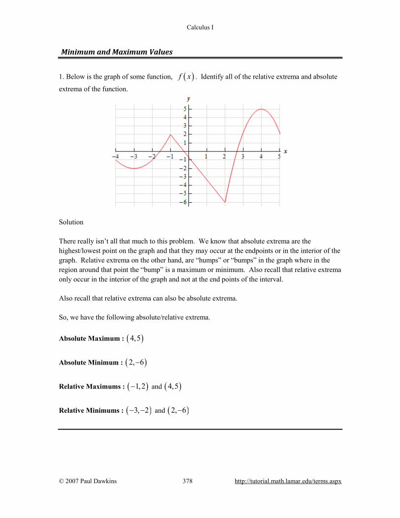
Calculus I
© 2007 Paul Dawkins 378 http://tutorial.math.lamar.edu/terms.aspx
Minimum and Maximum Values 1. Below is the graph of some function, ( )f x . Identify all of the relative extrema and absolute
extrema of the function.
Solution There really isn’t all that much to this problem. We know that absolute extrema are the highest/lowest point on the graph and that they may occur at the endpoints or in the interior of the graph. Relative extrema on the other hand, are “humps” or “bumps” in the graph where in the region around that point the “bump” is a maximum or minimum. Also recall that relative extrema only occur in the interior of the graph and not at the end points of the interval. Also recall that relative extrema can also be absolute extrema. So, we have the following absolute/relative extrema. Absolute Maximum : ( )4,5
Absolute Minimum : ( )2, 6−
Relative Maximums : ( )1, 2− and ( )4,5
Relative Minimums : ( )3, 2− − and ( )2, 6−

Calculus I
© 2007 Paul Dawkins 379 http://tutorial.math.lamar.edu/terms.aspx
2. Below is the graph of some function, ( )f x . Identify all of the relative extrema and absolute
extrema of the function.
Solution There really isn’t all that much to this problem. We know that absolute extrema are the highest/lowest point on the graph and that they may occur at the endpoints or in the interior of the graph. Relative extrema on the other hand, are “humps” or “bumps” in the graph where in the region around that point the “bump” is a maximum or minimum. Also recall that relative extrema only occur in the interior of the graph and not at the end points of the interval. Also recall that relative extrema can also be absolute extrema. So, we have the following absolute/relative extrema. Absolute Maximum : ( )6,8
Absolute Minimum : ( )9, 6−
Relative Maximums : ( )1,3 and ( )6,8
Relative Minimums : ( )2, 1− − and ( )2, 4−
3. Sketch the graph of ( ) 2 4g x x x= − and identify all the relative extrema and absolute extrema
of the function on each of the following intervals. (a) ( ),−∞ ∞
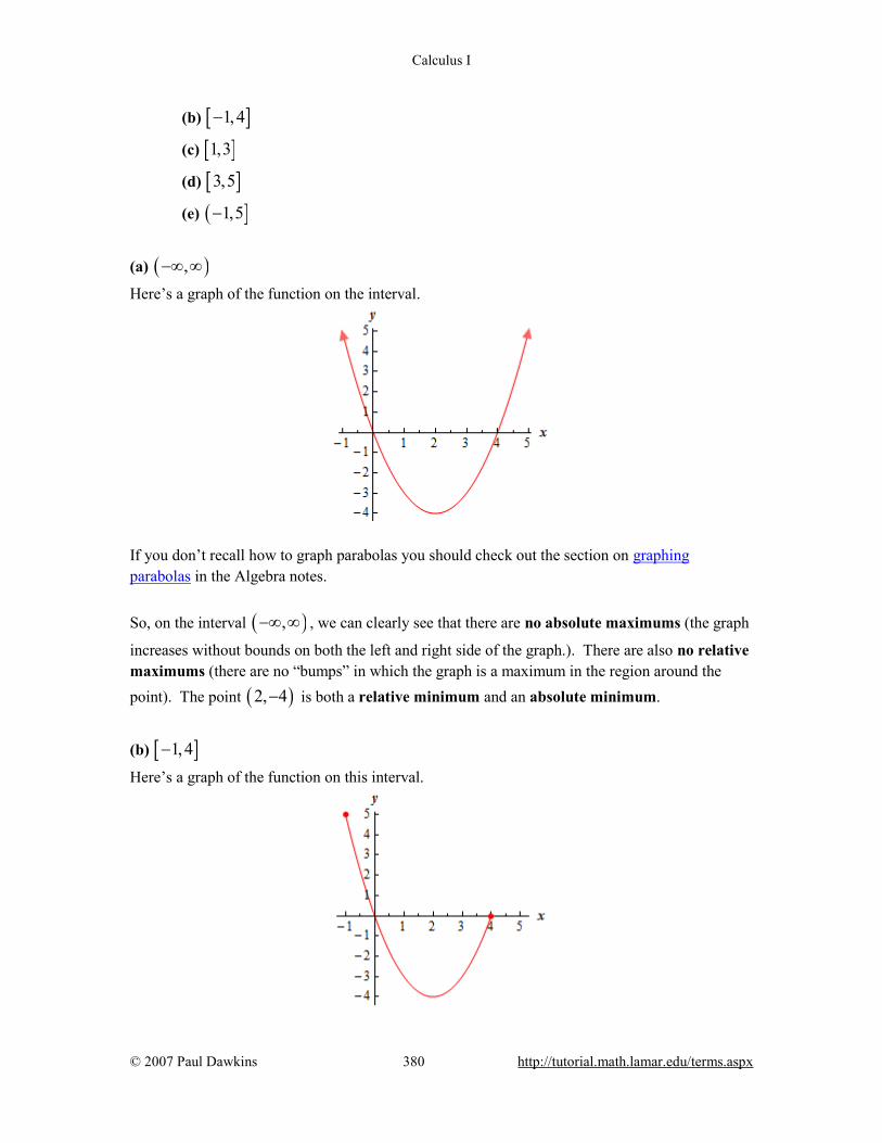
Calculus I
© 2007 Paul Dawkins 380 http://tutorial.math.lamar.edu/terms.aspx
(b) [ ]1, 4−
(c) [ ]1,3
(d) [ ]3,5
(e) ( ]1,5−
(a) ( ),−∞ ∞
Here’s a graph of the function on the interval.
If you don’t recall how to graph parabolas you should check out the section on graphing parabolas in the Algebra notes. So, on the interval ( ),−∞ ∞ , we can clearly see that there are no absolute maximums (the graph
increases without bounds on both the left and right side of the graph.). There are also no relative maximums (there are no “bumps” in which the graph is a maximum in the region around the point). The point ( )2, 4− is both a relative minimum and an absolute minimum.
(b) [ ]1, 4−
Here’s a graph of the function on this interval.
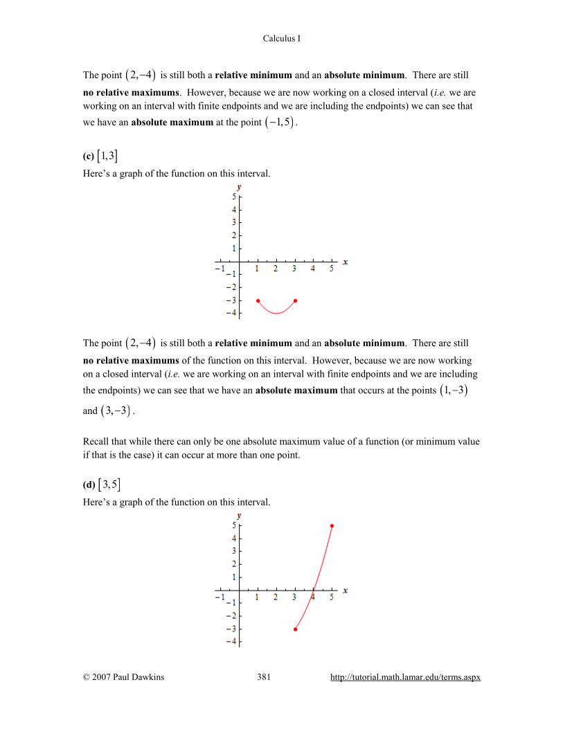
Calculus I
© 2007 Paul Dawkins 381 http://tutorial.math.lamar.edu/terms.aspx
The point ( )2, 4− is still both a relative minimum and an absolute minimum. There are still
no relative maximums. However, because we are now working on a closed interval (i.e. we are working on an interval with finite endpoints and we are including the endpoints) we can see that we have an absolute maximum at the point ( )1,5− .
(c) [ ]1,3
Here’s a graph of the function on this interval.
The point ( )2, 4− is still both a relative minimum and an absolute minimum. There are still
no relative maximums of the function on this interval. However, because we are now working on a closed interval (i.e. we are working on an interval with finite endpoints and we are including the endpoints) we can see that we have an absolute maximum that occurs at the points ( )1, 3−
and ( )3, 3− .
Recall that while there can only be one absolute maximum value of a function (or minimum value if that is the case) it can occur at more than one point. (d) [ ]3,5
Here’s a graph of the function on this interval.

Calculus I
© 2007 Paul Dawkins 382 http://tutorial.math.lamar.edu/terms.aspx
On this interval we clearly do not have any “bumps” in the interior of the interval and so, for this interval, there are no relative extrema of the function on this interval. However, we are working on a closed interval and so we can clearly see that there is an absolute maximum at the point
( )5,5 and an absolute minimum at the point ( )3, 3− .
(e) ( ]1,5−
Here’s a graph of the function on this interval.
The point ( )2, 4− is both a relative minimum and an absolute minimum. There are no
relative maximums of the function on this interval. For the absolute maximum we need to be a little careful however. In this case we are including the right endpoint of the interval, but not the left endpoint. Therefore, there is an absolute maximum at the point ( )5,5 . There is not, however, an absolute maximum at the left point
because that point is not being included in the interval. Because we are not including the left endpoint in the interval and so x will get closer and closer to
1x = − without actually reaching 1x = − . This means that while the graph will get closer and closer to 5y = it will never actually reach 5y = and so there will not be an absolute maximum at the left end point.
4. Sketch the graph of ( ) ( )34h x x= − + and identify all the relative extrema and absolute
extrema of the function on each of the following intervals. (a) ( ),−∞ ∞
(b) [ ]5.5, 2− −
(c) [ )4, 3− −

Calculus I
© 2007 Paul Dawkins 383 http://tutorial.math.lamar.edu/terms.aspx
(d) [ ]4, 3− −
(a) ( ),−∞ ∞
Here’s a graph of the function on the interval.
To graph this recall the transformations of graphs. The “-” in front simply reflects the graph of
3x about the x-axis and the “+4” shifts that graph 4 units to the left. So, on the interval ( ),−∞ ∞ , we can clearly see that there are no absolute maximums (the graph
increases/decreases without bounds on both the left/right side of the graph.). There are also no relative extrema (there are no “bumps” in which the graph is a maximum or minimum in the region around the point). Don’t get so locked into functions having to have extrema of some kind. There are all sorts of graphs that do not have absolute or relative extrema. This is one of those. (b) [ ]5.5, 2− −
Here’s a graph of the function on this interval.
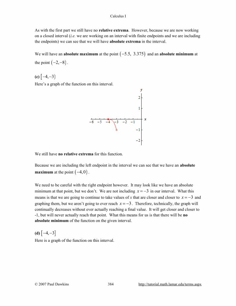
Calculus I
© 2007 Paul Dawkins 384 http://tutorial.math.lamar.edu/terms.aspx
As with the first part we still have no relative extrema. However, because we are now working on a closed interval (i.e. we are working on an interval with finite endpoints and we are including the endpoints) we can see that we will have absolute extrema in the interval. We will have an absolute maximum at the point ( )5.5, 3.375− and an absolute minimum at
the point ( )2, 8− − .
(c) [ )4, 3− −
Here’s a graph of the function on this interval.
We still have no relative extrema for this function. Because we are including the left endpoint in the interval we can see that we have an absolute maximum at the point ( )4,0− .
We need to be careful with the right endpoint however. It may look like we have an absolute minimum at that point, but we don’t. We are not including 3x = − in our interval. What this means is that we are going to continue to take values of x that are closer and closer to 3x = − and graphing them, but we aren’t going to ever reach 3x = − . Therefore, technically, the graph will continually decreases without ever actually reaching a final value. It will get closer and closer to -1, but will never actually reach that point. What this means for us is that there will be no absolute minimum of the function on the given interval. (d) [ ]4, 3− −
Here is a graph of the function on this interval.
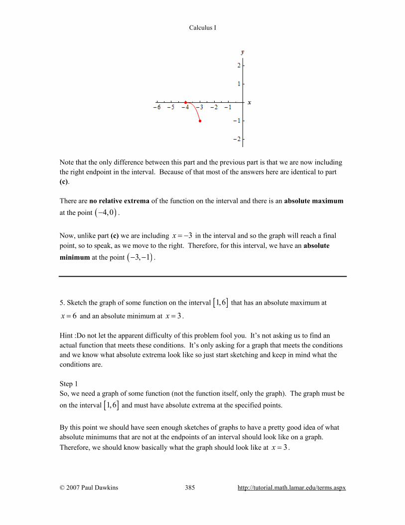
Calculus I
© 2007 Paul Dawkins 385 http://tutorial.math.lamar.edu/terms.aspx
Note that the only difference between this part and the previous part is that we are now including the right endpoint in the interval. Because of that most of the answers here are identical to part (c). There are no relative extrema of the function on the interval and there is an absolute maximum at the point ( )4,0− .
Now, unlike part (c) we are including 3x = − in the interval and so the graph will reach a final point, so to speak, as we move to the right. Therefore, for this interval, we have an absolute minimum at the point ( )3, 1− − .
5. Sketch the graph of some function on the interval [ ]1,6 that has an absolute maximum at
6x = and an absolute minimum at 3x = . Hint :Do not let the apparent difficulty of this problem fool you. It’s not asking us to find an actual function that meets these conditions. It’s only asking for a graph that meets the conditions and we know what absolute extrema look like so just start sketching and keep in mind what the conditions are. Step 1 So, we need a graph of some function (not the function itself, only the graph). The graph must be on the interval [ ]1,6 and must have absolute extrema at the specified points.
By this point we should have seen enough sketches of graphs to have a pretty good idea of what absolute minimums that are not at the endpoints of an interval should look like on a graph. Therefore, we should know basically what the graph should look like at 3x = .

Calculus I
© 2007 Paul Dawkins 386 http://tutorial.math.lamar.edu/terms.aspx
Next, we know that the absolute maximum must occur at the right end point of the interval and so all we need to do is sketch a curve from the absolute minimum up to the right endpoint and make sure that the graph at the right endpoint is simply higher than every other point on the graph. For the graph to the left of the absolute minimum we can sketch in pretty much anything until we reach the left end point, we just need to make sure that no portion of it goes below the absolute minimum or above the absolute maximum. Step 2 There are literally an infinite number of graphs that we could do here. Some will be more complicated that others, but here is probably one of the simpler graphs that we could use here.
6. Sketch the graph of some function on the interval [ ]4,3− that has an absolute maximum at
3x = − and an absolute minimum at 2x = . Hint :Do not let the apparent difficulty of this problem fool you. It’s not asking us to find an actual function that meets these conditions. It’s only asking for a graph that meets the conditions and we know what absolute extrema look like so just start sketching and keep in mind what the conditions are. Step 1 So, we need a graph of some function (not the function itself, only the graph). The graph must be on the interval [ ]4,3− and must have absolute extrema at the specified points.
By this point we should have seen enough sketches of graphs to have a pretty good idea of what absolute maximums/minimums that are not at the endpoints of an interval should look like on a graph. Therefore, we should know basically what the graph should look like at 3x = − and

Calculus I
© 2007 Paul Dawkins 387 http://tutorial.math.lamar.edu/terms.aspx
2x = . There are many ways we could sketch the graph between these two points, but there is no reason to overly complicate the graph so the best thing to do is probably just sketch in a short smooth curve connecting the two points. Also, because the absolute extrema occur interior to the interval we know that the graph at the endpoints of the interval must fall somewhere between the maximum/minimum values of the graph. This means that as we sketch the graph from the absolute maximum to the left end point we can sketch anything we just need to make sure it never rises above the highest point on the graph or below the lowest point on the graph. Similarly as we sketch the graph from the absolute minimum to the right endpoint we just need to make sure it stays between the highest and lowest point on the graph. Step 2 There are literally an infinite number of graphs that we could do here. Some will be more complicated that others, but here is probably one of the simpler graphs that we could use here.
7. Sketch the graph of some function that meets the following conditions :
(a) The function is continuous. (b) Has two relative minimums. (b) One of relative minimums is also an absolute minimum and the other relative
minimum is not an absolute minimum. (c) Has one relative maximum. (d) Has no absolute maximum.
Hint :Do not let the apparent difficulty of this problem fool you. It’s not asking us to find an actual function that meets these conditions. It’s only asking for a graph that meets the conditions
Calculus I
© 2007 Paul Dawkins 388 http://tutorial.math.lamar.edu/terms.aspx
and we know what absolute and relative extrema look like so just start sketching and keep in mind what the conditions are. Step 1 So, we need a graph of some function (not the function itself, only the graph) that meets the given conditions. We were not given an interval as one of the conditions so it’s okay to assume that the interval is ( ),−∞ ∞ for this problem.
From the first condition we know that we can’t have any holes or breaks in the graph in order for the function to be continuous. Now let’s take care of the next two conditions as they are related to each other. By this point we’ve seen enough sketches of graphs to have a pretty good idea of what absolute and relative minimums looks like. So, we’re going to need two downwards pointing “bumps” in the graph to give use the two relative minimums. Also, one of them must be the lowest point on the graph and other must be higher so it is not also an absolute minimum. Next, we want to think about how to connect the two relative minimums. This is also where the fourth condition comes in. As we’ll see because we have a continuous function we’ll need that to connect the two relative minimums. Let’s start with the leftmost relative minimum. In order for it to be a minimum the graph must be increasing as we move to the right. However, if we also want to get the minimum to the right of this the graph will have to, at some point, start decreasing again. If you think about it that is exactly what a relative maximum will look like. So, in moving from the leftmost relative minimum to the rightmost relative minimum we must have a relative maximum between them and so the fourth condition is automatically met. Note that if we don’t insist on a continuous function it is possible to get from one to the other without having a relative minimum. All it would take is to have a division by zero discontinuity somewhere between the two relative minimums in which the graph goes to positive infinity on both sides of the discontinuity. This would maintain the relative minimums and at the same time would not be a relative maximum. Now let’s deal with the final condition. In order for the graph to have no absolute maximum all we really need to do is make sure that the graph increases without bound as we move to the right and left of the graph. This will also match up nicely with the relative minimums that we are required to have. To the left of the leftmost relative minimum the graph must be increasing and so we may as well just let it increase forever on that side. Likewise, on the right side of the rightmost relative

Calculus I
© 2007 Paul Dawkins 389 http://tutorial.math.lamar.edu/terms.aspx
minimum the graph will need to be increasing. So, again let’s just let the graph increase forever on that side. Step 2 There are literally an infinite number of graphs that we could do here. Some will be more complicated that others, but here is probably one of the simpler graphs that we could use here.
Finding Absolute Extrema 1. Determine the absolute extrema of ( ) 3 28 81 42 8f x x x x= + − − on [ ]8,2− .
Hint : Just recall the process for finding absolute extrema outlined in the notes for this section and you’ll be able to do this problem! Step 1 First, notice that we are working with a polynomial and this is continuous everywhere and so will be continuous on the given interval. Recall that this is important because we now know that absolute extrema will in fact exist by the Extreme Value Theorem! Now that we know that absolute extrema will in fact exist on the given interval we’ll need to find the critical points of the function. Given that the purpose of this section is to find absolute extrema we’ll not be putting much work/explanation into the critical point steps. If you need practice finding critical points please go back and work some problems from that section.
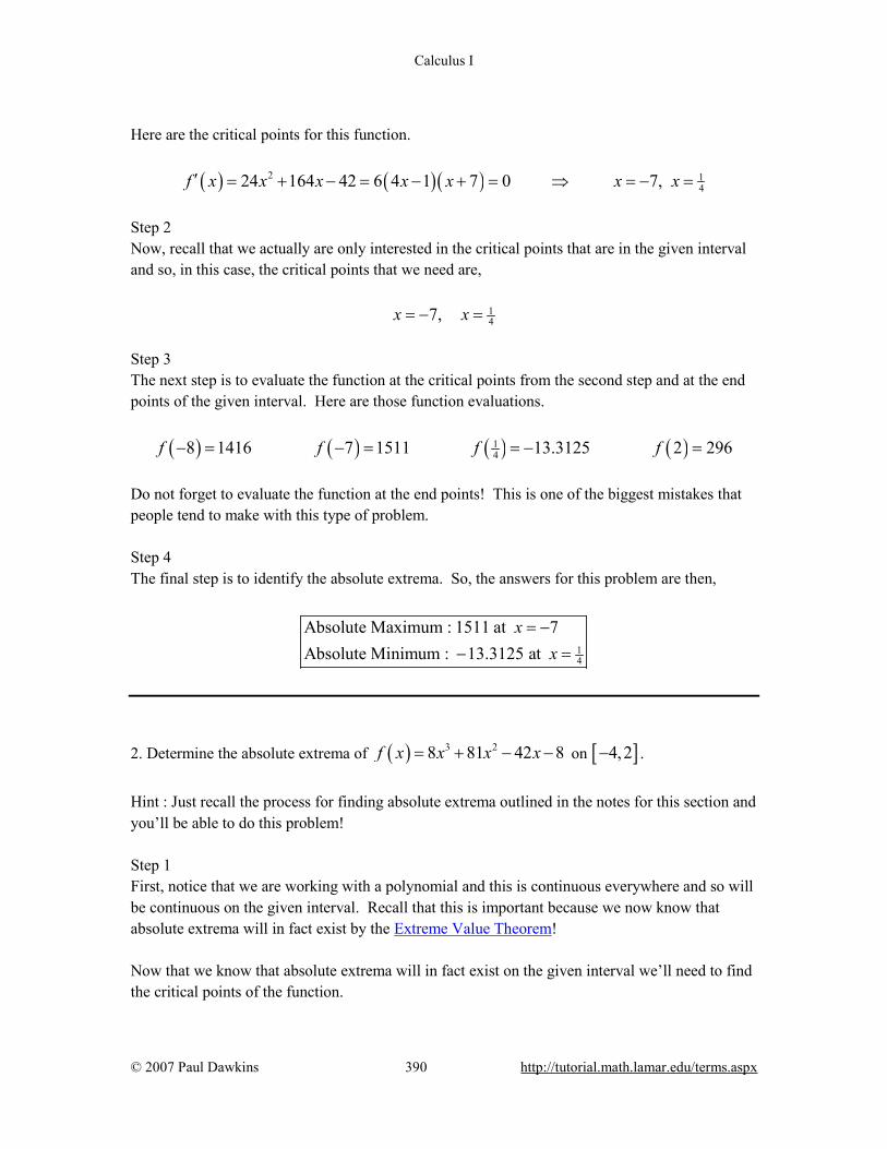
Calculus I
© 2007 Paul Dawkins 390 http://tutorial.math.lamar.edu/terms.aspx
Here are the critical points for this function. ( ) ( )( )2 1
424 164 42 6 4 1 7 0 7,f x x x x x x x′ = + − = − + = ⇒ = − = Step 2 Now, recall that we actually are only interested in the critical points that are in the given interval and so, in this case, the critical points that we need are, 1
47,x x= − = Step 3 The next step is to evaluate the function at the critical points from the second step and at the end points of the given interval. Here are those function evaluations. ( ) ( ) ( ) ( )1
48 1416 7 1511 13.3125 2 296f f f f− = − = = − = Do not forget to evaluate the function at the end points! This is one of the biggest mistakes that people tend to make with this type of problem. Step 4 The final step is to identify the absolute extrema. So, the answers for this problem are then,
14
Absolute Maximum : 1511 at 7Absolute Minimum : 13.3125 at
xx
= −− =
2. Determine the absolute extrema of ( ) 3 28 81 42 8f x x x x= + − − on [ ]4,2− .
Hint : Just recall the process for finding absolute extrema outlined in the notes for this section and you’ll be able to do this problem! Step 1 First, notice that we are working with a polynomial and this is continuous everywhere and so will be continuous on the given interval. Recall that this is important because we now know that absolute extrema will in fact exist by the Extreme Value Theorem! Now that we know that absolute extrema will in fact exist on the given interval we’ll need to find the critical points of the function.

Calculus I
© 2007 Paul Dawkins 391 http://tutorial.math.lamar.edu/terms.aspx
Given that the purpose of this section is to find absolute extrema we’ll not be putting much work/explanation into the critical point steps. If you need practice finding critical points please go back and work some problems from that section. Here are the critical points for this function. ( ) ( )( )2 1
424 164 42 6 4 1 7 0 7,f x x x x x x x′ = + − = − + = ⇒ = − = Step 2 Now, recall that we actually are only interested in the critical points that are in the given interval and so, in this case, the only critical point that we need is, 1
4x = Step 3 The next step is to evaluate the function at the critical point from the second step and at the end points of the given interval. Here are those function evaluations. ( ) ( ) ( )1
44 944 13.3125 2 296f f f− = = − = Do not forget to evaluate the function at the end points! This is one of the biggest mistakes that people tend to make with this type of problem. Step 4 The final step is to identify the absolute extrema. So, the answers for this problem are then,
14
Absolute Maximum : 944 at 4Absolute Minimum : 13.3125 at
xx
= −− =
Note the importance of paying attention to the interval with this problem. Had we neglected to exclude 7x = − we would have gotten the wrong answer for the absolute maximum (check out the previous problem to see this….). 3. Determine the absolute extrema of ( ) 3 4 51 80 5 2R t t t t= + + − on [ ]4.5, 4− .
Hint : Just recall the process for finding absolute extrema outlined in the notes for this section and you’ll be able to do this problem! Step 1

Calculus I
© 2007 Paul Dawkins 392 http://tutorial.math.lamar.edu/terms.aspx
First, notice that we are working with a polynomial and this is continuous everywhere and so will be continuous on the given interval. Recall that this is important because we now know that absolute extrema will in fact exist by the Extreme Value Theorem! Now that we know that absolute extrema will in fact exist on the given interval we’ll need to find the critical points of the function. Given that the purpose of this section is to find absolute extrema we’ll not be putting much work/explanation into the critical point steps. If you need practice finding critical points please go back and work some problems from that section. Here are the critical points for this function. ( ) ( )( )2 3 4 2240 20 10 10 6 4 0 4, 0, 6R t t t t t t t t t t′ = + − = − − + = ⇒ = − = = Step 2 Now, recall that we actually are only interested in the critical points that are in the given interval and so, in this case, the critical points that we need are, 4, 0t t= − = Step 3 The next step is to evaluate the function at the critical points from the second step and at the end points of the given interval. Here are those function evaluations. ( ) ( ) ( ) ( )4.5 1548.13 4 1791 0 1 4 4353R R R R− = − − = − = = Do not forget to evaluate the function at the end points! This is one of the biggest mistakes that people tend to make with this type of problem. Step 4 The final step is to identify the absolute extrema. So, the answers for this problem are then,
Absolute Maximum : 4353 at 4Absolute Minimum : 1791 at 4
tt=
− = −
Note the importance of paying attention to the interval with this problem. Had we neglected to exclude 6t = we would have gotten the wrong answer for the absolute maximum. Also note that if we’d neglected to check the endpoints at all we also would have gotten the wrong absolute maximum.

Calculus I
© 2007 Paul Dawkins 393 http://tutorial.math.lamar.edu/terms.aspx
4. Determine the absolute extrema of ( ) 3 4 51 80 5 2R t t t t= + + − on [ ]0,7 .
Hint : Just recall the process for finding absolute extrema outlined in the notes for this section and you’ll be able to do this problem! Step 1 First, notice that we are working with a polynomial and this is continuous everywhere and so will be continuous on the given interval. Recall that this is important because we now know that absolute extrema will in fact exist by the Extreme Value Theorem! Now that we know that absolute extrema will in fact exist on the given interval we’ll need to find the critical points of the function. Given that the purpose of this section is to find absolute extrema we’ll not be putting much work/explanation into the critical point steps. If you need practice finding critical points please go back and work some problems from that section. Here are the critical points for this function. ( ) ( )( )2 3 4 2240 20 10 10 6 4 0 4, 0, 6R t t t t t t t t t t′ = + − = − − + = ⇒ = − = = Step 2 Now, recall that we actually are only interested in the critical points that are in the given interval and so, in this case, the critical points that we need are, 0, 6t t= = Do not get excited about the fact that one of the critical points also happens to be one of the end points of the interval. This happens on occasion. Step 3 The next step is to evaluate the function at the critical points from the second step and at the end points of the given interval. Here are those function evaluations. ( ) ( ) ( )0 1 6 8209 7 5832R R R= = = Do not forget to evaluate the function at the end points! This is one of the biggest mistakes that people tend to make with this type of problem. Step 4 The final step is to identify the absolute extrema. So, the answers for this problem are then,

Calculus I
© 2007 Paul Dawkins 394 http://tutorial.math.lamar.edu/terms.aspx
Absolute Maximum : 8209 at 6Absolute Minimum : 1 at 0
tt
==
Note the importance of paying attention to the interval with this problem. Had we neglected to exclude 4t = − we would have gotten the wrong answer for the absolute minimum. 5. Determine the absolute extrema of ( ) 3 24 3 9 12h z z z z= − + + on [ ]2,1− .
Hint : Just recall the process for finding absolute extrema outlined in the notes for this section and you’ll be able to do this problem! Step 1 First, notice that we are working with a polynomial and this is continuous everywhere and so will be continuous on the given interval. Recall that this is important because we now know that absolute extrema will in fact exist by the Extreme Value Theorem! Now that we know that absolute extrema will in fact exist on the given interval we’ll need to find the critical points of the function. Given that the purpose of this section is to find absolute extrema we’ll not be putting much work/explanation into the critical point steps. If you need practice finding critical points please go back and work some problems from that section. Here are the critical points for this function.
( ) 2 6 396 1 1112 6 9 024 4
ih z z z z ± − ±′ = − + = ⇒ = = Now, recall that we only work with real numbers here and so we ignore complex roots. Therefore this function has no critical points. Step 2 Technically the next step is to determine all the critical points that are in the given interval. However, there are no critical points for this function and so there are also no critical points in the given interval. Step 3 The next step is to evaluate the function at the critical points from the second step and at the end points of the given interval. However, since there are no critical points for this function all we need to do is evaluate the function at the end points of the interval.

Calculus I
© 2007 Paul Dawkins 395 http://tutorial.math.lamar.edu/terms.aspx
Here are those function evaluations. ( ) ( )2 50 1 22h h− = − = Do not forget to evaluate the function at the end points! This is one of the biggest mistakes that people tend to make with this type of problem. That is especially true for this problem as there would be no points to evaluate at without the end points. Step 4 The final step is to identify the absolute extrema. So, the answers for this problem are then,
Absolute Maximum : 22 at 1Absolute Minimum : 50 at 2
zz=
− = −
Note that if we hadn’t remembered to evaluate the function at the end points of the interval we would not have had an answer for this problem! 6. Determine the absolute extrema of ( ) 4 3 23 26 60 11g x x x x= − + − on [ ]1,5 .
Hint : Just recall the process for finding absolute extrema outlined in the notes for this section and you’ll be able to do this problem! Step 1 First, notice that we are working with a polynomial and this is continuous everywhere and so will be continuous on the given interval. Recall that this is important because we now know that absolute extrema will in fact exist by the Extreme Value Theorem! Now that we know that absolute extrema will in fact exist on the given interval we’ll need to find the critical points of the function. Given that the purpose of this section is to find absolute extrema we’ll not be putting much work/explanation into the critical point steps. If you need practice finding critical points please go back and work some problems from that section. Here are the critical points for this function. ( ) ( ) ( )3 2 5
212 78 120 6 4 2 5 0 0, , 4g x x x x x x x x x x′ = − + = − − = ⇒ = = = Step 2

Calculus I
© 2007 Paul Dawkins 396 http://tutorial.math.lamar.edu/terms.aspx
Now, recall that we actually are only interested in the critical points that are in the given interval and so, in this case, the critical points that we need are, 5
2 , 4x x= = Step 3 The next step is to evaluate the function at the critical points from the second step and at the end points of the given interval. Here are those function evaluations. ( ) ( ) ( ) ( )5
21 26 74.9375 4 53 5 114g g g g= = = = Do not forget to evaluate the function at the end points! This is one of the biggest mistakes that people tend to make with this type of problem. Step 4 The final step is to identify the absolute extrema. So, the answers for this problem are then,
Absolute Maximum : 114 at 5Absolute Minimum : 26 at 1
xx
==
Note that if we hadn’t remembered to evaluate the function at the end points of the interval we would have gotten both of the answers incorrect!
7. Determine the absolute extrema of ( ) ( ) ( )34 22 8 9Q x x x= − − on [ ]3,3− .
Hint : Just recall the process for finding absolute extrema outlined in the notes for this section and you’ll be able to do this problem! Step 1 First, notice that we are working with a polynomial and this is continuous everywhere and so will be continuous on the given interval. Recall that this is important because we now know that absolute extrema will in fact exist by the Extreme Value Theorem! Now that we know that absolute extrema will in fact exist on the given interval we’ll need to find the critical points of the function. Given that the purpose of this section is to find absolute extrema we’ll not be putting much work/explanation into the critical point steps. If you need practice finding critical points please go back and work some problems from that section.

Calculus I
© 2007 Paul Dawkins 397 http://tutorial.math.lamar.edu/terms.aspx
Here are the critical points for this function.
( ) ( ) ( ) ( ) ( )( ) ( )( ) ( ) ( )
3 23 42 2
23 2 2
3 579614 40
4 8 2 8 9 3 2 2 8 9
4 2 8 9 20 3 72
0 , 3, 1.8239, 1.9739
Q x x x x x x
x x x x
x x x ±
′ = − − − + − −
= − − − − −
= ⇒ = = ± = = −
Step 2 Now, recall that we actually are only interested in the critical points that are in the given interval and so, in this case, we need all the critical points from the first step.
3 579614 40, 3, 1.8239, 1.9739x x x ±= = ± = = −
Do not get excited about the fact that both end points of the interval are also critical points. It happens sometimes and in this case it will reduce the number of computations required in the next step by 2 and that’s not a bad thing. Step 3 The next step is to evaluate the function at the critical points from the second step and at the end points of the given interval. Here are those function evaluations. ( ) ( ) ( ) ( ) ( )7 61
43 0 1.8239 1.38 10 0 1.9739 4.81 10 3 0Q Q Q Q Q− = − = − × = = − × = Do not get excited about the large numbers for the two non-zero function values. This is something that is going to happen on occasion and we shouldn’t worry about it when it does happen. Step 4 The final step is to identify the absolute extrema. So, the answers for this problem are then,
14
7
Absolute Maximum : 0 at 3, , 3
Absolute Minimum : 1.38 10 at 1.8239
x x x
x
= − = =
− × = − Recall that while we can only have one largest possible value (i.e. only one absolute maximum) it is completely possible for it to occur at more than one point (3 points in this case).
8. Determine the absolute extrema of ( ) ( )532 2h w w w= + on 5 12 2,− .
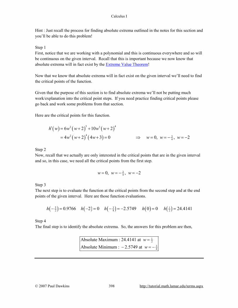
Calculus I
© 2007 Paul Dawkins 398 http://tutorial.math.lamar.edu/terms.aspx
Hint : Just recall the process for finding absolute extrema outlined in the notes for this section and you’ll be able to do this problem! Step 1 First, notice that we are working with a polynomial and this is continuous everywhere and so will be continuous on the given interval. Recall that this is important because we now know that absolute extrema will in fact exist by the Extreme Value Theorem! Now that we know that absolute extrema will in fact exist on the given interval we’ll need to find the critical points of the function. Given that the purpose of this section is to find absolute extrema we’ll not be putting much work/explanation into the critical point steps. If you need practice finding critical points please go back and work some problems from that section. Here are the critical points for this function.
( ) ( ) ( )
( ) ( )
5 42 3
42 34
6 2 10 2
4 2 4 3 0 0, , 2
h w w w w w
w w w w w w
′ = + + +
= + + = ⇒ = = − = −
Step 2 Now, recall that we actually are only interested in the critical points that are in the given interval and so, in this case, we need all the critical points from the first step. 3
40, , 2w w w= = − = − Step 3 The next step is to evaluate the function at the critical points from the second step and at the end points of the given interval. Here are those function evaluations. ( ) ( ) ( ) ( ) ( )5 3 1
2 4 20.9766 2 0 2.5749 0 0 24.4141h h h h h− = − = − = − = = Step 4 The final step is to identify the absolute extrema. So, the answers for this problem are then,
12
34
Absolute Maximum : 24.4141 at Absolute Minimum : 2.5749 at
ww
=
− = −

Calculus I
© 2007 Paul Dawkins 399 http://tutorial.math.lamar.edu/terms.aspx
9. Determine the absolute extrema of ( ) 2
42 8
zf zz z
+=
+ + on [ ]10,0− .
Hint : Just recall the process for finding absolute extrema outlined in the notes for this section and you’ll be able to do this problem! Step 1 First, notice that we are working with a rational expression in which both the numerator and denominator are continuous everywhere. Also notice that the rational expression exists at all points in the interval and so will be continuous on the given interval. Recall that this is important because we now know that absolute extrema will in fact exist by the Extreme Value Theorem! Now that we know that absolute extrema will in fact exist on the given interval we’ll need to find the critical points of the function. Given that the purpose of this section is to find absolute extrema we’ll not be putting much work/explanation into the critical point steps. If you need practice finding critical points please go back and work some problems from that section. Here are the critical points for this function.
( )( )( ) ( ) ( )
( )( )
( )
2
22
28 72
222
1 2 8 4 4 1
2 8
2 8 20 4 3 2 8.2426, 0.2426
2 8
z z z zf z
z z
z zz
z z− ±
+ + − + +′ =
+ +
− + −= = ⇒ = = − ± = −
+ +
Step 2 Now, recall that we actually are only interested in the critical points that are in the given interval and so, in this case, the only critical point that we need is,
4 3 2 8.2426z = − − = − Step 3 The next step is to evaluate the function at the critical point from the second step and at the end points of the given interval. Here are those function evaluations. ( ) ( ) ( )1 1
33 210 0.0303 8.2426 0.03128 0f f f− = − = − − = − = Step 4 The final step is to identify the absolute extrema. So, the answers for this problem are then,
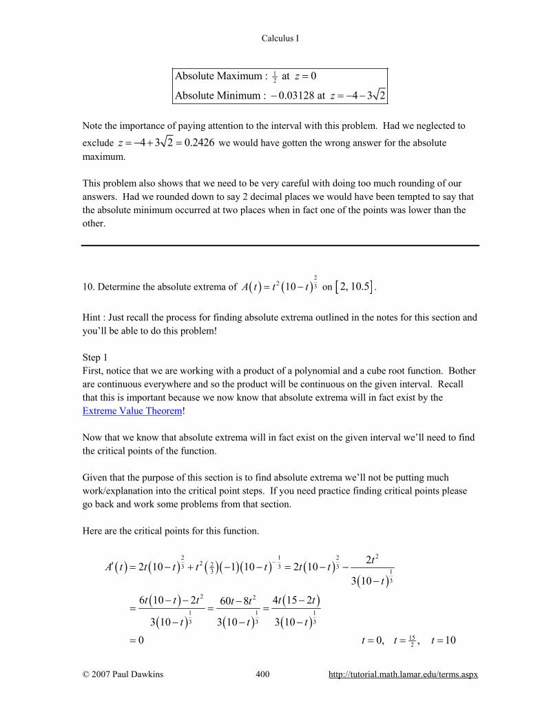
Calculus I
© 2007 Paul Dawkins 400 http://tutorial.math.lamar.edu/terms.aspx
12Absolute Maximum : at 0
Absolute Minimum : 0.03128 at 4 3 2
z
z
=
− = − − Note the importance of paying attention to the interval with this problem. Had we neglected to
exclude 4 3 2 0.2426z = − + = we would have gotten the wrong answer for the absolute maximum. This problem also shows that we need to be very careful with doing too much rounding of our answers. Had we rounded down to say 2 decimal places we would have been tempted to say that the absolute minimum occurred at two places when in fact one of the points was lower than the other.
10. Determine the absolute extrema of ( ) ( )2
2 310A t t t= − on [ ]2, 10.5 .
Hint : Just recall the process for finding absolute extrema outlined in the notes for this section and you’ll be able to do this problem! Step 1 First, notice that we are working with a product of a polynomial and a cube root function. Bother are continuous everywhere and so the product will be continuous on the given interval. Recall that this is important because we now know that absolute extrema will in fact exist by the Extreme Value Theorem! Now that we know that absolute extrema will in fact exist on the given interval we’ll need to find the critical points of the function. Given that the purpose of this section is to find absolute extrema we’ll not be putting much work/explanation into the critical point steps. If you need practice finding critical points please go back and work some problems from that section. Here are the critical points for this function.
( ) ( ) ( )( ) ( ) ( )( )
( )( ) ( )
( )( )
22 1 22 23 3 3
3 13
2 2
1 1 13 3 3
152
22 10 1 10 2 103 10
6 10 2 4 15 260 8
3 10 3 10 3 100 0, , 10
tA t t t t t t tt
t t t t tt t
t t tt t t
−′ = − + − − = − −−
− − −−= = =
− − −
= = = =
Calculus I
© 2007 Paul Dawkins 401 http://tutorial.math.lamar.edu/terms.aspx
Don’t forget about critical points where the derivative doesn’t exist! Step 2 Now, recall that we actually are only interested in the critical points that are in the given interval and so, in this case, the critical points that we need are, 15
2 , 10t t= = Step 3 The next step is to evaluate the function at the critical points from the second step and at the end points of the given interval. Here are those function evaluations. ( ) ( ) ( ) ( )15
22 16 103.613 10 0 10.5 69.4531A A A A= = = = Step 4 The final step is to identify the absolute extrema. So, the answers for this problem are then,
152Absolute Maximum : 103.613 at
Absolute Minimum : 0 at 10t
t=
=
Note the importance of paying attention to the interval with this problem. Had we neglected to exclude 0t = we would have had the absolute minimum showing up at two places instead of only the one place inside the given interval.
11. Determine the absolute extrema of ( ) ( )3 92sin y yf y = + on [ ]10,15− .
Hint : Just recall the process for finding absolute extrema outlined in the notes for this section and you’ll be able to do this problem! Step 1 First, notice that we are working with the sine function and this is continuous everywhere and so will be continuous on the given interval. Recall that this is important because we now know that absolute extrema will in fact exist by the Extreme Value Theorem! Now that we know that absolute extrema will in fact exist on the given interval we’ll need to find the critical points of the function.
Calculus I
© 2007 Paul Dawkins 402 http://tutorial.math.lamar.edu/terms.aspx
Given that the purpose of this section is to find absolute extrema we’ll not be putting much work/explanation into the critical point steps. If you need practice finding critical points please go back and work some problems from that section. Here are the critical points for this function.
( ) ( ) ( ) ( )11 2 23 3 9 3 3 3 3
2cos 0 cos cos 2.3005y y yf y −′ = + = → = − → = − =
3
3
2.3005 2 6.9016 60, 1, 2, ,
11.9481 63.9827 2
y
yn y n
ny nn
π πππ
= + = +⇒ = ± ± ±
= += +…
If you need some review on solving trig equations please go back to the Review chapter and work some of the problems the Solving Trig Equations sections. Step 2 Now, recall that we actually are only interested in the critical points that are in the given interval and so, in this case, the critical points that we need are, 6.9016, 6.9016, 11.9481y y y= − = = Note that we got these values by plugging in values of n into the solutions above and checking the results against the given interval. Step 3 The next step is to evaluate the function at the critical points from the second step and at the end points of the given interval. Here are those function evaluations.
( ) ( ) ( )
( ) ( )10 2.0317 6.9016 2.2790 6.9016 2.2790
11.9481 1.9098 15 2.3744
f f f
f f
− = − − = − =
= =
Step 4 The final step is to identify the absolute extrema. So, the answers for this problem are then,
Absolute Maximum : 2.3744 at 15Absolute Minimum : 2.2790 at 6.9016
yy=
− = −
Note the importance of paying attention to the interval with this problem. Without an interval we would have had (literally) an infinite number of critical points to check. Also, without an interval (as a quick graph of the function would show) there would be no absolute extrema for this function.
Calculus I
© 2007 Paul Dawkins 403 http://tutorial.math.lamar.edu/terms.aspx
12. Determine the absolute extrema of ( ) 3 22 7w w wg w − −= e on 512 2,− .
Hint : Just recall the process for finding absolute extrema outlined in the notes for this section and you’ll be able to do this problem! Step 1 First, notice that we are working with an exponential function with a polynomial in the exponent. The exponent is continuous everywhere and so we can see that the exponential function will also be continuous everywhere. Therefore the function will be continuous on the given interval. Recall that this is important because we now know that absolute extrema will in fact exist by the Extreme Value Theorem! Now that we know that absolute extrema will in fact exist on the given interval we’ll need to find the critical points of the function. Given that the purpose of this section is to find absolute extrema we’ll not be putting much work/explanation into the critical point steps. If you need practice finding critical points please go back and work some problems from that section. Here are the critical points for this function.
( ) ( )
( )( )
3 2
3 2
2 2 7
2 7 73
3 4 7
1 3 7 0 1,
w w w
w w w
g w w w
w w w w
− −
− −
′ = − −
= + − = ⇒ = − =
e
e
Step 2 Now, recall that we actually are only interested in the critical points that are in the given interval and so, in this case, the only critical point that we need is, 7
3w = Step 3 The next step is to evaluate the function at the critical point from the second step and at the end points of the given interval. Here are those function evaluations.
( ) ( ) ( )23 392 1158 27 87 51
2 3 2g g g− −− = = =e e e Step 4 The final step is to identify the absolute extrema. So, the answers for this problem are then,
Calculus I
© 2007 Paul Dawkins 404 http://tutorial.math.lamar.edu/terms.aspx
238
39227
12
73
Absolute Maximum : at
Absolute Minimum : at
w
w−
= −
=
e
e Note the importance of paying attention to the interval with this problem. Had we neglected to exclude 1w = − we would have gotten the absolute maximum wrong. Also note that we need to be careful with rounding with this problem. Both of the exponentials with negative exponents are very small and rounding could cause some real issues here. However, we don’t need to actually do any calculator work for this anyway. Recall that the more negative the exponent is the smaller the exponential will be.
So, because 392 11527 8> we must have
392 11527 8− −<e e .
13. Determine the absolute extrema of ( ) ( )2ln 4 14R x x x= + + on [ ]4,2− .
Hint : Just recall the process for finding absolute extrema outlined in the notes for this section and you’ll be able to do this problem! Step 1 First, notice that we are working with a logarithm whose argument is a polynomial (which is continuous everywhere) that is always positive in the interval. Because of this we can see that the function will be continuous on the given interval. Recall that this is important because we now know that absolute extrema will in fact exist by the Extreme Value Theorem! Now that we know that absolute extrema will in fact exist on the given interval we’ll need to find the critical points of the function. Given that the purpose of this section is to find absolute extrema we’ll not be putting much work/explanation into the critical point steps. If you need practice finding critical points please go back and work some problems from that section. Here are the critical points for this function.
( ) 2
2 4 24 14xR x x
x x+′ = ⇒ = −
+ +
Step 2 Now, recall that we actually are only interested in the critical points that are in the given interval and so, in this case, the critical point that we need is,
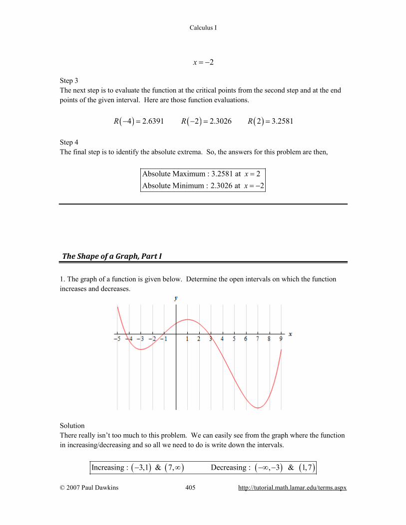
Calculus I
© 2007 Paul Dawkins 405 http://tutorial.math.lamar.edu/terms.aspx
2x = − Step 3 The next step is to evaluate the function at the critical points from the second step and at the end points of the given interval. Here are those function evaluations. ( ) ( ) ( )4 2.6391 2 2.3026 2 3.2581R R R− = − = = Step 4 The final step is to identify the absolute extrema. So, the answers for this problem are then,
Absolute Maximum : 3.2581 at 2Absolute Minimum : 2.3026 at 2
xx
== −
The Shape of a Graph, Part I 1. The graph of a function is given below. Determine the open intervals on which the function increases and decreases.
Solution There really isn’t too much to this problem. We can easily see from the graph where the function in increasing/decreasing and so all we need to do is write down the intervals.
( ) ( ) ( ) ( )Increasing : 3,1 & 7, Decreasing : , 3 & 1,7− ∞ −∞ −

Calculus I
© 2007 Paul Dawkins 406 http://tutorial.math.lamar.edu/terms.aspx
Note as well that by open intervals we mean that we don’t include the end points in the interval. For this problem that is important because at the end points we are at infinity or the function is either not increasing or decreasing. 2. The graph of a function is given below. Determine the open intervals on which the function increases and decreases.
Solution There really isn’t too much to this problem. We can easily see from the graph where the function in increasing/decreasing and so all we need to do is write down the intervals.
( ) ( ) ( ) ( )Increasing : ,1 , 4,8 & 8, Decreasing : 1, 4−∞ ∞ Note as well that by open intervals we mean that we don’t include the end points in the interval. For this problem that is important because at the end points we are at infinity or the function is either not increasing or decreasing. 3. Below is the graph of the derivative of a function. From this graph determine the open intervals in which the function increases and decreases.

Calculus I
© 2007 Paul Dawkins 407 http://tutorial.math.lamar.edu/terms.aspx
Hint : Be careful with this problem. The graph is of the derivative of the function and so we don’t just write down intervals where the graph is increasing and decreasing. Recall how the derivative tells us where the function is increasing and decreasing and this problem is not too bad. Solution We have to be careful and not do this problem as we did the first two practice problems. The graph given is the graph of the derivative and not the graph of the function. So, the answer is not just where the graph is increasing or decreasing. Instead we need to recall that the sign of the derivative tells us where the function is increasing and decreasing. If the derivative is positive (i.e. its graph is above the x-axis) then the function is increasing and if the derivative is negative (i.e. its graph is below the x-axis) then the function is decreasing. So, it is fairly clear where the graph is above/below the x-axis and so we have the following intervals of increase/decrease.
( ) ( ) ( ) ( )Increasing : 7, 2 & 2,5 Decreasing : , 7 & 5,− − − −∞ − ∞
4. This problem is about some function. All we know about the function is that it exists everywhere and we also know the information given below about the derivative of the function. Answer each of the following questions about this function.
(a) Identify the critical points of the function. (b) Determine the open intervals on which the function increases and decreases. (c) Classify the critical points as relative maximums, relative minimums or neither.
Calculus I
© 2007 Paul Dawkins 408 http://tutorial.math.lamar.edu/terms.aspx
( ) ( ) ( ) ( )( ) ( ) ( ) ( ) ( ) ( ) ( )
5 0 2 0 4 0 8 0
0 on 5, 2 , 2,4 , 8, 0 on , 5 , 4,8
f f f f
f x f x
′ ′ ′ ′− = − = = =
′ ′< − − − ∞ > −∞ −
Hint : This problem is actually quite simple. Just keep in mind how critical points are defined and how we can answer the last two parts from the derivative of the function. (a) Identify the critical points of the function. Okay, let’s recall the definition of a critical point. A critical point is any point in which the function exists and the derivative is either zero or doesn’t exist. We are given that the function exists everywhere (and in fact this part is why that in there at all….) and so we don’t really need to worry about that part of the definition for this problem. Also, from the given information about the derivative we can see that at every point the derivative is either zero, positive or negative. In other words, the derivative will exist at every point. So, all this means that the critical points of the function are those points were the derivative is zero and we are given those in the information. Therefore, the critical points of the function are,
5, 2, 4, 8x x x x= − = − = =
(b) Determine the open intervals on which the function increases and decreases. There is really not a lot to this part. We know that the function will increase where the derivative is positive and it will decrease where the derivative is negative. This positive and negative information is clearly listed above in the given information so here are the increasing/decreasing intervals for this function.
( ) ( ) ( ) ( ) ( )Increasing : , 5 & 4,8 Decreasing : 5, 2 , 2,4 & 8,−∞ − − − − ∞ (c) Classify the critical points as relative maximums, relative minimums or neither. Okay, there isn’t a lot that we need to do here. We know that relative maximums are increasing on the left and decreasing on the right and relative minimums are decreasing on the left and increasing on the right. We have all the increasing/decreasing information from the second part so here is the answer to this part.
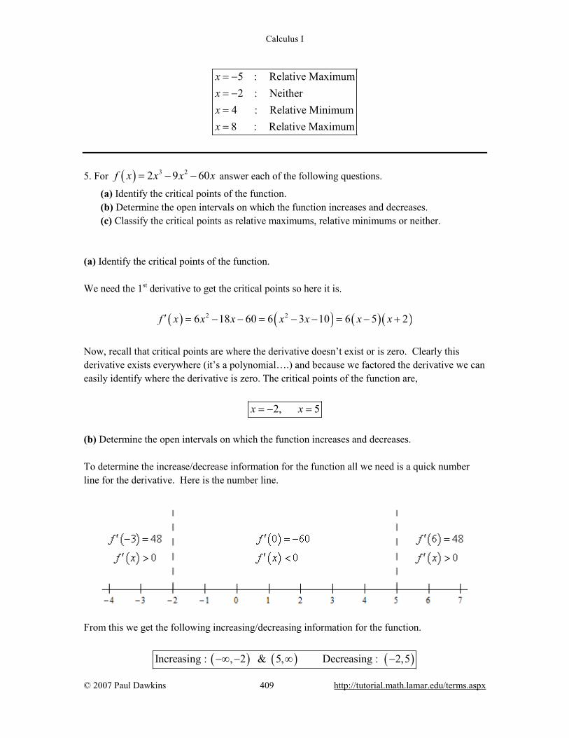
Calculus I
© 2007 Paul Dawkins 409 http://tutorial.math.lamar.edu/terms.aspx
5 : Relative Maximum2 : Neither
4 : Relative Minimum8 : Relative Maximum
xxxx
= −= −==
5. For ( ) 3 22 9 60f x x x x= − − answer each of the following questions.
(a) Identify the critical points of the function. (b) Determine the open intervals on which the function increases and decreases. (c) Classify the critical points as relative maximums, relative minimums or neither.
(a) Identify the critical points of the function. We need the 1st derivative to get the critical points so here it is.
( ) ( ) ( )( )2 26 18 60 6 3 10 6 5 2f x x x x x x x′ = − − = − − = − +
Now, recall that critical points are where the derivative doesn’t exist or is zero. Clearly this derivative exists everywhere (it’s a polynomial….) and because we factored the derivative we can easily identify where the derivative is zero. The critical points of the function are,
2, 5x x= − =
(b) Determine the open intervals on which the function increases and decreases. To determine the increase/decrease information for the function all we need is a quick number line for the derivative. Here is the number line.
From this we get the following increasing/decreasing information for the function.
( ) ( ) ( )Increasing : , 2 & 5, Decreasing : 2,5−∞ − ∞ −

Calculus I
© 2007 Paul Dawkins 410 http://tutorial.math.lamar.edu/terms.aspx
(c) Classify the critical points as relative maximums, relative minimums or neither. With the increasing/decreasing information from the previous step we can easily classify the critical points using the 1st derivative test. Here is classification of the functions critical points.
2 : Relative Maximum
5 : Relative Minimumxx
= −=
6. For ( ) 3 4 550 40 5 4h t t t t= + − − answer each of the following questions.
(a) Identify the critical points of the function. (b) Determine the open intervals on which the function increases and decreases. (c) Classify the critical points as relative maximums, relative minimums or neither.
(a) Identify the critical points of the function. We need the 1st derivative to get the critical points so here it is.
( ) ( ) ( )( )2 3 4 2 2 2120 20 20 20 6 20 3 2h t t t t t t t t t t′ = − − = − + − = − + −
Now, recall that critical points are where the derivative doesn’t exist or is zero. Clearly this derivative exists everywhere (it’s a polynomial….) and because we factored the derivative we can easily identify where the derivative is zero. The critical points of the function are,
3, 0, 2t t t= − = =
(b) Determine the open intervals on which the function increases and decreases. To determine the increase/decrease information for the function all we need is a quick number line for the derivative. Here is the number line.
Calculus I
© 2007 Paul Dawkins 411 http://tutorial.math.lamar.edu/terms.aspx
From this we get the following increasing/decreasing information for the function.
( ) ( ) ( ) ( )Increasing : 3,0 & 0, 2 Decreasing : , 3 & 2,− −∞ − ∞ (c) Classify the critical points as relative maximums, relative minimums or neither. With the increasing/decreasing information from the previous step we can easily classify the critical points using the 1st derivative test. Here is classification of the functions critical points.
3 : Relative Minimum
0 : Neither5 : Relative Maximum
ttt
= −==
7. For 3 22 10 12 12y x x x= − + − answer each of the following questions.
(a) Identify the critical points of the function. (b) Determine the open intervals on which the function increases and decreases. (c) Classify the critical points as relative maximums, relative minimums or neither.
(a) Identify the critical points of the function. We need the 1st derivative to get the critical points so here it is.
26 20 12dy x xdx
= − +
Now, recall that critical points are where the derivative doesn’t exist or is zero. Clearly this derivative exists everywhere (it’s a polynomial….) and because the derivative can’t be factored in this case we’ll need to do a quick quadratic formula to find where the derivative is zero. The critical points of the function are,
5 7 0.78475, 2.548583
x ±= =
(b) Determine the open intervals on which the function increases and decreases. To determine the increase/decrease information for the function all we need is a quick number line for the derivative. Here is the number line.

Calculus I
© 2007 Paul Dawkins 412 http://tutorial.math.lamar.edu/terms.aspx
From this we get the following increasing/decreasing information for the function.
( ) ( ) ( )5 7 5 7 5 7 5 73 3 3 3Increasing : , & , Decreasing : ,− + − +−∞ ∞
(c) Classify the critical points as relative maximums, relative minimums or neither. With the increasing/decreasing information from the previous step we can easily classify the critical points using the 1st derivative test. Here is classification of the functions critical points.
5 7
3
5 73
0.78475 : Relative Maximum
2.54858 : Relative Minimum
x
x
−
+
= =
= =
8. For ( ) ( )cos 3 2p x x x= + answer each of the following questions on 3
2 , 2− .
(a) Identify the critical points of the function. (b) Determine the open intervals on which the function increases and decreases. (c) Classify the critical points as relative maximums, relative minimums or neither.
(a) Identify the critical points of the function. We need the 1st derivative to get the critical points so here it is.
( ) ( )3sin 3 2p x x′ = − +
Now, recall that critical points are where the derivative doesn’t exist or is zero. Clearly this derivative exists everywhere (the sine function exists everywhere….) and so all we need to do is set the derivative equal to zero and solve. We’re not going to show all of those details so if you need to do some review of the process go back to the Solving Trig Equations sections for some examples. Here are all the critical points.

Calculus I
© 2007 Paul Dawkins 413 http://tutorial.math.lamar.edu/terms.aspx
23
23
0.24320, 1, 2, 3,
0.8040x n
nx n
π
π
= += ± ± ±
= +…
Plugging in some n’s gives the following critical points in the interval 3
2 , 2− .
1.2904, 0.2432, 0.8040x x x= − = =
(b) Determine the open intervals on which the function increases and decreases. To determine the increase/decrease information for the function all we need is a quick number line for the derivative. Here is the number line.
From this we get the following increasing/decreasing information for the function.
( ) ( ]
) ( )32
Increasing : 1.2904,0.2432 & 0.8040, 2
Decreasing : , 1.2904 & 0.2432,0.8040
−
− − Be careful with the end points of these intervals! We are working on the interval 3
2 , 2− and
we’ve done no work for increasing and decreasing outside of this interval and so we can’t say anything about what happens outside of the interval. (c) Classify the critical points as relative maximums, relative minimums or neither. With the increasing/decreasing information from the previous step we can easily classify the critical points using the 1st derivative test. Here is classification of the functions critical points.
1.2904 : Relative Minimum
0.2432 : Relative Maximum0.8040 : Relative Minimum
xxx
= −==
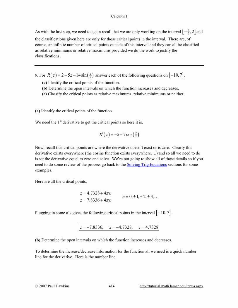
Calculus I
© 2007 Paul Dawkins 414 http://tutorial.math.lamar.edu/terms.aspx
As with the last step, we need to again recall that we are only working on the interval 32 , 2− and
the classifications given here are only for those critical points in the interval. There are, of course, an infinite number of critical points outside of this interval and they can all be classified as relative minimums or relative maximums provided we do the work to justify the classifications. 9. For ( ) ( )22 5 14sin zR z z= − − answer each of the following questions on [ ]10,7− .
(a) Identify the critical points of the function. (b) Determine the open intervals on which the function increases and decreases. (c) Classify the critical points as relative maximums, relative minimums or neither.
(a) Identify the critical points of the function. We need the 1st derivative to get the critical points so here it is.
( ) ( )25 7 cos zR z′ = − −
Now, recall that critical points are where the derivative doesn’t exist or is zero. Clearly this derivative exists everywhere (the cosine function exists everywhere….) and so all we need to do is set the derivative equal to zero and solve. We’re not going to show all of those details so if you need to do some review of the process go back to the Solving Trig Equations sections for some examples. Here are all the critical points.
4.7328 4
0, 1, 2, 3,7.8336 4
z nn
z nππ
= += ± ± ±
= +…
Plugging in some n’s gives the following critical points in the interval [ ]10,7− .
7.8336, 4.7328, 4.7328z z z= − = − =
(b) Determine the open intervals on which the function increases and decreases. To determine the increase/decrease information for the function all we need is a quick number line for the derivative. Here is the number line.

Calculus I
© 2007 Paul Dawkins 415 http://tutorial.math.lamar.edu/terms.aspx
From this we get the following increasing/decreasing information for the function.
( ) ( ][ ) ( )
Increasing : 7.8336, 4.7328 & 4.7328,7
Decreasing : 10, 7.8336 & 4.7328, 4.7328
− −
− − − Be careful with the end points of these intervals! We are working on the interval [ ]10,7− and
we’ve done no work for increasing and decreasing outside of this interval and so we can’t say anything about what happens outside of the interval. (c) Classify the critical points as relative maximums, relative minimums or neither. With the increasing/decreasing information from the previous step we can easily classify the critical points using the 1st derivative test. Here is classification of the functions critical points.
7.8336 : Relative Minimum4.7328 : Relative Maximum
4.7328 : Relative Minimum
zzz
= −= −=
As with the last step, we need to again recall that we are only working on the interval [ ]10,7−
and the classifications given here are only for those critical points in the interval. There are, of course, an infinite number of critical points outside of this interval and they can all be classified as relative minimums or relative maximums provided we do the work to justify the classifications.
10. For ( ) 2 3 7h t t t= − answer each of the following questions.
(a) Identify the critical points of the function. (b) Determine the open intervals on which the function increases and decreases. (c) Classify the critical points as relative maximums, relative minimums or neither.
(a) Identify the critical points of the function.
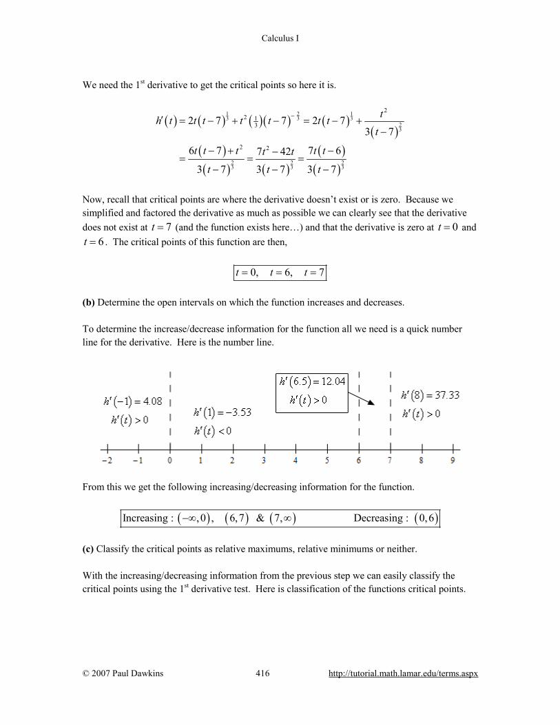
Calculus I
© 2007 Paul Dawkins 416 http://tutorial.math.lamar.edu/terms.aspx
We need the 1st derivative to get the critical points so here it is.
( ) ( ) ( )( ) ( )( )
( )( ) ( )
( )( )
1 2 13 3 3
23
2 2 23 3 3
22 1
3
2 2
2 7 7 2 73 7
6 7 7 67 42
3 7 3 7 3 7
th t t t t t t tt
t t t t tt tt t t
−′ = − + − = − +−
− + −−= = =
− − −
Now, recall that critical points are where the derivative doesn’t exist or is zero. Because we simplified and factored the derivative as much as possible we can clearly see that the derivative does not exist at 7t = (and the function exists here…) and that the derivative is zero at 0t = and
6t = . The critical points of this function are then,
0, 6, 7t t t= = =
(b) Determine the open intervals on which the function increases and decreases. To determine the increase/decrease information for the function all we need is a quick number line for the derivative. Here is the number line.
From this we get the following increasing/decreasing information for the function.
( ) ( ) ( ) ( )Increasing : ,0 , 6,7 & 7, Decreasing : 0,6−∞ ∞ (c) Classify the critical points as relative maximums, relative minimums or neither. With the increasing/decreasing information from the previous step we can easily classify the critical points using the 1st derivative test. Here is classification of the functions critical points.

Calculus I
© 2007 Paul Dawkins 417 http://tutorial.math.lamar.edu/terms.aspx
0 : Relative Maximum6 : Relative Minimum7 : Neither
ttt
===
11. For ( )21
22 wf w w −= e answer each of the following questions.
(a) Identify the critical points of the function. (b) Determine the open intervals on which the function increases and decreases. (c) Classify the critical points as relative maximums, relative minimums or neither.
(a) Identify the critical points of the function. We need the 1st derivative to get the critical points so here it is.
( ) ( ) ( ) ( )2 2 2 21 1 1 1
2 2 2 22 2 2 22 21 1 1w w w wf w w w w w− − − −′ = − = − = − +e e e e
Now, recall that critical points are where the derivative doesn’t exist or is zero. Because we simplified and factored the derivative as much as possible we can clearly see that the derivative will exist everywhere (it’s the product of functions that exist everywhere). We can also easily see where the derivative is zero. The critical points of this function are then,
1, 1w w= − =
(b) Determine the open intervals on which the function increases and decreases. To determine the increase/decrease information for the function all we need is a quick number line for the derivative. Here is the number line.
From this we get the following increasing/decreasing information for the function.

Calculus I
© 2007 Paul Dawkins 418 http://tutorial.math.lamar.edu/terms.aspx
( ) ( ) ( )Increasing : 1,1 Decreasing : , 1 & 1,− −∞ − ∞ (c) Classify the critical points as relative maximums, relative minimums or neither. With the increasing/decreasing information from the previous step we can easily classify the critical points using the 1st derivative test. Here is classification of the functions critical points.
1 : Relative Minimum
1 : Relative Maximumww
= −=
12. For ( ) ( )22ln 1g x x x= − + answer each of the following questions.
(a) Identify the critical points of the function. (b) Determine the open intervals on which the function increases and decreases. (c) Classify the critical points as relative maximums, relative minimums or neither.
(a) Identify the critical points of the function. We need the 1st derivative to get the critical points so here it is.
( )2
2 2
2 1 41 21 1
x x xg xx x
− += − =
+ +
Now, recall that critical points are where the derivative doesn’t exist or is zero. Because we simplified and factored the derivative as much as possible we can clearly see that the derivative will exist everywhere (or at least the denominator will not be zero for any real numbers…). We’ll also need the quadratic formula to determine where the numerator, and hence the derivative, is zero. The critical points of this function are then,
2 3 0.2679, 3.7321x = ± =
(b) Determine the open intervals on which the function increases and decreases. To determine the increase/decrease information for the function all we need is a quick number line for the derivative. Here is the number line.
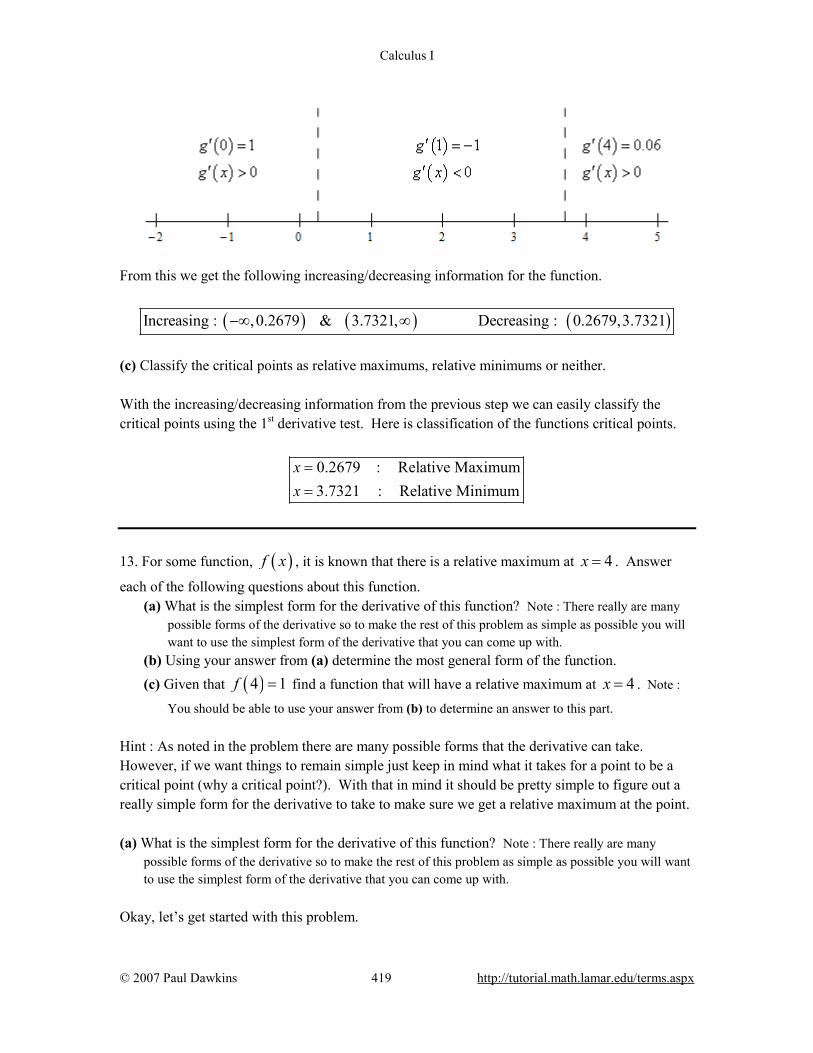
Calculus I
© 2007 Paul Dawkins 419 http://tutorial.math.lamar.edu/terms.aspx
From this we get the following increasing/decreasing information for the function.
( ) ( ) ( )Increasing : ,0.2679 & 3.7321, Decreasing : 0.2679,3.7321−∞ ∞ (c) Classify the critical points as relative maximums, relative minimums or neither. With the increasing/decreasing information from the previous step we can easily classify the critical points using the 1st derivative test. Here is classification of the functions critical points.
0.2679 : Relative Maximum3.7321 : Relative Minimum
xx
==
13. For some function, ( )f x , it is known that there is a relative maximum at 4x = . Answer
each of the following questions about this function. (a) What is the simplest form for the derivative of this function? Note : There really are many
possible forms of the derivative so to make the rest of this problem as simple as possible you will want to use the simplest form of the derivative that you can come up with.
(b) Using your answer from (a) determine the most general form of the function. (c) Given that ( )4 1f = find a function that will have a relative maximum at 4x = . Note :
You should be able to use your answer from (b) to determine an answer to this part. Hint : As noted in the problem there are many possible forms that the derivative can take. However, if we want things to remain simple just keep in mind what it takes for a point to be a critical point (why a critical point?). With that in mind it should be pretty simple to figure out a really simple form for the derivative to take to make sure we get a relative maximum at the point. (a) What is the simplest form for the derivative of this function? Note : There really are many
possible forms of the derivative so to make the rest of this problem as simple as possible you will want to use the simplest form of the derivative that you can come up with.
Okay, let’s get started with this problem.
Calculus I
© 2007 Paul Dawkins 420 http://tutorial.math.lamar.edu/terms.aspx
The first thing that we’ll do is assume that the derivative exists everywhere. Making assumptions in a math class is generally a bad thing. However, in this case, because we are being asked to come up the form of the derivative all we are really doing here is starting that process. If we can’t find a derivative that will have a relative maximum at the point that also exists everywhere we can come back and change things up. If we can find a derivative that will exist everywhere (which we can as we’ll see) this assumption will help with keeping the derivative as simple as possible. Now, given that we are assuming that the derivative exists everywhere and we know that if we have a relative maximum at 4x = then 4x = must also be a critical point (recall Fermat’s Theorem from a couple of sections ago…). This is another reason for the assumption we made above. Fermat’s theorem requires that the derivative exist at the point in order to know that it is also a critical point. Next, because we assumed that the derivative exists everywhere (and in particular it exists at
4x = ) we know that in order for it to be a critical point we must also have ( )4 0f ′ = . There are
lots and lots of functions that will be zero at 4x = but probably one of the simplest is use,
( ) 4f x x′ = − This does give ( )4 0f ′ = as we need, however we have a problem. We can clearly see that if
4x < we would have ( ) 0f x′ < and if 4x > we would have ( ) 0f x′ > . This says that 4x =
would have to be a relative minimum and not the relative maximum that we wanted it to be. Luckily enough for us this is easy to fix. The only problem with our original guess is that the signs of the derivative to the right and left of 4x = are opposite what we need them to be. Therefore, all we need to do is change them and that can easily be done by multiplying by a negative or,
( ) 4f x x′ = −
With this choice we still have ( )4 0f ′ = and now the derivative is positive if 4x < and negative
if 4x > which means that 4x = will be a relative maximum. As noted in the problem statement there are many possible answers to this part. We will be working with the one given above. However, just to make the point here are a sampling of other derivatives all of which come from functions that have a relative maximum at 4x = . ( ) ( ) ( ) ( ) ( )2 2 416 24 18 6 1 sin 2xf x x f x x x f x f x xπ π−′ ′ ′ ′= − = + − = − = −e

Calculus I
© 2007 Paul Dawkins 421 http://tutorial.math.lamar.edu/terms.aspx
After working the rest of this problem with ( ) 4f x x′ = − you might want to come back and see
if you can repeat the problem with one or more of these to see what you get. Hint : This is where the problem gets a little tricky (as if the previous part wasn’t tricky huh?). What we need to do here is “undo” the derivative. However, if you kept the answer from the previous part simple and you understand how differentiation works then it shouldn’t be too hard to “undo” the differentiation and determine a function that gives your derivative. Keep in mind however that the problem statement asks for the most general possible function and that is where most will run into problems with this part. (b) Using your answer from (a) determine the most general form of the function. Okay, from the previous part we have assumed that the derivative of our function is
( ) 4f x x′ = − and we need to “undo” the differentiation to determine the most general possible
function that we could have had. So, before doing this let’s recall what we know about differentiation. First, let’s recall the following formula,
( ) 1n nd x nxdx
−=
When we differentiate a power of x the power goes down by one. So, what would we have to differentiate to get x? We’ll, since the exponent on the x is 1 we would have had to differentiate an 2x . However, because we know that that the derivative of 2x is 2x and we want just an x that would mean that in fact we would have had to differentiate 21
2 x to get x. Next, also recall,
( )d kx kdx
=
So, using this as a guide is should be pretty simple to see that we would need to differentiate 4x to get 4. So, if we put these two parts together it looks like we could use the following function. ( ) 21
24f x x x= − The derivative of this function is clearly ( ) 4f x x′ = − . However, it is not the most general
possible function that gives this derivative.
Calculus I
© 2007 Paul Dawkins 422 http://tutorial.math.lamar.edu/terms.aspx
Do not forget that the derivative of a constant is zero and so we could add any constant onto our function and get the same derivative. This is one of the biggest mistakes that students make with learning to “undo” differentiation. Any time we undo differentiation there is always the possibility that there was a constant on the original function and so we need to acknowledge that. We usually do this by adding a “ + c ” onto the end of our function. We use a general c because we have no way of knowing that the constant would be and this allows for all possible constants. Therefore, the most general function that we could use to get ( ) 4f x x′ = − is,
( ) 2124f x x x c= − +
Hint : This is the “easy” part of this problem. All we are really being asked to do is determine the specific value of c that we would need in order have the function have the value of 1 at 4x = . If you’ve reached this point of a Calculus course you should have the required Algebra knowledge (and yes it really is just Algebra) to do this part. (c) Given that ( )4 1f = find a function that will have a relative maximum at 4x = . Note : You
should be able to use your answer from (b) to determine an answer to this part. To do this part all we really need to do is plug 4x = into our answer from the previous part and set the result equal to 1. This will result in an equation with a single unknown value, c. So all we need to do then is solve for c. Here is the work for this part.
( ) ( ) ( )2121 4 4 4 4 8 1 8 7f c c c c= = − + = + → = + → = −
So, it looks like one possible function that will have a relative maximum at 4x = is,
( ) 2124 7f x x x= − −
As a final part to this problem, here is a quick graph of this function to verify that it does in fact have a relative maximum at 4x = .

Calculus I
© 2007 Paul Dawkins 423 http://tutorial.math.lamar.edu/terms.aspx
14. Given that ( )f x and ( )g x are increasing functions. If we define ( ) ( ) ( )h x f x g x= +
show that ( )h x is an increasing function.
Hint : At first glance this problem may seem quite difficult. However, just keep in mind how we have been determining whether functions where increasing to this point and that should suggest a first step. Step 1 To this point we’ve always used the derivative to determine if a function was increasing so let’s do that here as well. Note that this may not seem all that useful because we don’t actually know what any of the functions are. However, just because we don’t know what the functions are doesn’t mean that we can’t at least write down a formula for ( )h x′ . Here is that formula.
( ) ( ) ( )h x f x g x′ ′ ′= + Hint : We were told that ( )f x and ( )g x are increasing functions so what does that tell us about
their derivatives? Step 2 We are told that both ( )f x and ( )g x are increasing functions so this means that we know that
both of their derivatives must be positive. Or, ( ) ( )0 0f x g x′ ′> >
Calculus I
© 2007 Paul Dawkins 424 http://tutorial.math.lamar.edu/terms.aspx
Hint : Given the formula for ( )h x′ we found in Step 1 and what we noticed about the signs of
( )f x′ and ( )g x′ that we noted in Step 2 what can we say about the sign of ( )h x ?
Step 3 Okay, we are pretty much done at this point. We know from Step 1 that, ( ) ( ) ( )h x f x g x′ ′ ′= + Also from Step 2 we know that both ( )f x′ and ( )g x′ are positive. So, ( )h x′ is the sum of
two positive functions and in turn means that we must have, ( ) 0h x′ > Therefore we can see that ( )h x must be an increasing function.
-------------------------------------------------------
Final Thoughts / Strategy Discussion Figuring out how to do these kinds of problems can definitely seem quite daunting at times. That is especially true when the statement we are being asked to prove seems to be fairly "obvious" as is the case here. The sum of two increasing functions intuitively should also be increasing. The problem is that we are being asked to actually prove that and not just say "well it makes sense so it should be true". What we want to discuss here is not the proof of this fact (that is given above after all...). Instead let's take a look at the thought process that went into constructing the proof above. The first step is to really look at what we are being asked to prove. This means not just reading the statement, but reading the statement and trying to relate what we are being asked to prove to something we already know. In this case, we’re being asked to show that a general function is increasing given a set of assumptions. By this point we know how to prove that specific functions are increasing. So, let’s start with that. We know that in order to use Calculus to prove that a function is increasing we need to look at the derivative of the function. We also know that, at least symbolically, we write down the formula for the derivative of the function we are interested in for this problem. Now for the next step in the thought process. We've got a formula and we know that we need to show that it is positive. At this point we need to think about the assumptions that we were given.
Calculus I
© 2007 Paul Dawkins 425 http://tutorial.math.lamar.edu/terms.aspx
Don't forget the assumptions. They were given for a reason and we'll need to use them. What do the assumptions tell us? How can we relate them to what we are being asked to prove? In this case, we know from the assumptions that the two derivatives were positive. For this problem this wasn't a particularly difficult step, but for other problems this can be a little tricky. Finally, we need to put the two previous thought process steps together. This can also be a fairly tricky step. If you haven't had a lot of exposure to "mathematical logic/proofs" it can be daunting to put all the information together. Often times you will need to try various ways of putting the information together before something "clicks" and you can see how to proceed. You may even need to go back to the previous step and see if there is something about the assumptions that you may have missed. In this case we could see that the derivative was the sum of two other derivatives and from our assumptions we knew that the two individual derivatives had to be positive. We also know from basic Algebra knowledge that the sum of two positive quantities has to be positive and so we are done. The key part of this whole process is that you will have to persevere. Try not to get discouraged and if something doesn't work out move on and try something else. Also, do not get so wrapped up in the process that you don't take breaks occasionally. If you keep running into road blocks then step away for a while and come back at a later point. Sometimes that is all it takes to get a fresh idea. Another thing that students often initially have difficulty with is trying to mathematically write this kind of thing down. In your mind you may have been able to see all the "logic" involved in the proof, but just couldn't see who to put it all together and write it down. If you are having that problem the best thing to do is just start writing things down. For instance, you know you need the derivative of the given function so write that down. If you don't have a specific function to differentiate can you at least symbolically write down the derivative as we did here? Once you have that written down look at the pieces and start writing down what you know about them. Actually write down what you know (i.e. things like ( ) 0f x′ > ). This seems silly at
times, but it really can help with the process. Once you have everything written down you might be able to see how to string everything together with words/explanations to prove what you want to prove.

Calculus I
© 2007 Paul Dawkins 426 http://tutorial.math.lamar.edu/terms.aspx
15. Given that ( )f x is an increasing function and define ( ) ( ) 2h x f x= . Will ( )h x be an
increasing function? If yes, prove that ( )h x is an increasing function. If not, can you determine
any other conditions needed on the function ( )f x that will guarantee that ( )h x will also
increase? Hint : If you have trouble with these kinds of “proof” problems you might want to check out the discussion at the end of the previous problem for a “strategy” that might be useful here. This isn’t quite the same kind of problem but the strategy given there should help here as well. Hint : How do we use Calculus to determine if a function is increasing? Step 1 We know that the derivative can be used to tell us if a function is increasing so let’s find the derivative of ( )h x . Do not get excited about the fact that we don’t know what ( )f x is. We
can symbolically take the derivative with a quick application of the chain rule. Here is the derivative of ( )h x .
( ) ( ) ( ) ( ) ( )2 2h x f x f x f x f x1
′ ′ ′= = Hint : How do we use the derivative to determine if a function is increasing? Step 2 We know that a function will be increasing if its derivative is positive. So, the question we need to answer is can we guarantee that ( ) 0h x′ > if we only take into account the assumption that
( )f x is an increasing function.
From our assumption that ( )f x is an increasing function and so we know that ( ) 0f x′ > .
Now, let’s see what ( )h x′ tells us. We can see that ( )h x′ is a product of a number and two
functions. The “2” is positive and so the sign of the derivative will come from the sign of the product of ( )f x and ( )f x′ .
Hint : So, will ( )h x′ be positive?
Step 3

Calculus I
© 2007 Paul Dawkins 427 http://tutorial.math.lamar.edu/terms.aspx
Okay, from our assumption we know that ( )f x′ is positive. However, the product isn’t
guaranteed to be positive. For example, consider ( )f x x= . Clearly, ( ) 1 0f x′ = > , and so this is an increasing function.
However, ( ) ( ) ( )( )1f x f x x x′ = = . Therefore, we can see that the product will not always be
positive. This shouldn’t be too surprising given that,
( ) ( ) [ ]2 2 2h x f x x x= = =
In this case we can clearly see that ( )h x will not always be an increasing function.
On the other had if we let ( ) xf x = e we can see that ( ) 0xf x′ = >e and we can also see that
( ) ( ) ( )( ) 2 0x x xf x f x′ = = >e e e .
So, from these two examples we can see that we can find increasing functions, ( )f x , for which
( ) 2f x may or may not always be increasing.
Hint : Can you use the examples above to determine a condition on ( )f x that will guarantee that
( )h x will be increasing?
Step 4 So, just what was the difference between the two examples above? The problem with the first example, ( )f x x= was that it wasn’t always positive and so the
product of ( )f x and ( )f x′ would not always be positive as we needed it to be.
This was not a problem with the second example however, ( ) xf x = e . In this case the function
is always positive and so the product of the function and its derivative will also be positive. That is also the added condition that we need to guarantee that ( )h x will be positive.
If we start with the assumption that ( )f x in an increasing function we need to further assume
that ( )f x is a positive function in order to guarantee that ( ) ( ) 2h x f x= will be a positive
function.

Calculus I
© 2007 Paul Dawkins 428 http://tutorial.math.lamar.edu/terms.aspx
The Shape of a Graph, Part II 1. The graph of a function is given below. Determine the open intervals on which the function is concave up and concave down.
Solution There really isn’t too much to this problem. We can easily see from the graph where the function in concave up/concave down and so all we need to do is estimate where the concavity changes (and this really will be an estimate as it won’t always be clear) and write down the intervals.
( ) ( ) ( ) ( )Concave Up : 1,2 & 6, Concave Down : , 1 & 2,6− ∞ −∞ − Again, the endpoints of these intervals are, at best, estimates as it won’t always be clear just where the concavity changes. 2. Below is the graph the 2nd derivative of a function. From this graph determine the open intervals in which the function is concave up and concave down.
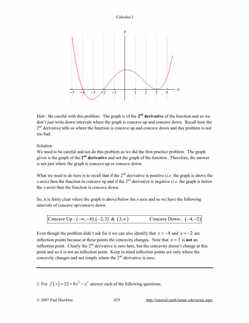
Calculus I
© 2007 Paul Dawkins 429 http://tutorial.math.lamar.edu/terms.aspx
Hint : Be careful with this problem. The graph is of the 2nd derivative of the function and so we don’t just write down intervals where the graph is concave up and concave down. Recall how the 2nd derivative tells us where the function is concave up and concave down and this problem is not too bad. Solution We need to be careful and not do this problem as we did the first practice problem. The graph given is the graph of the 2nd derivative and not the graph of the function. Therefore, the answer is not just where the graph is concave up or concave down. What we need to do here is to recall that if the 2nd derivative is positive (i.e. the graph is above the x-axis) then the function in concave up and if the 2nd derivative is negative (i.e. the graph is below the x-axis) then the function is concave down. So, it is fairly clear where the graph is above/below the x-axis and so we have the following intervals of concave up/concave down.
( ) ( ) ( ) ( )Concave Up : , 4 , 2,3 & 3, Concave Down : 4, 2−∞ − − ∞ − − Even though the problem didn’t ask for it we can also identify that 4x = − and 2x = − are inflection points because at these points the concavity changes. Note that 3x = is not an inflection point. Clearly the 2nd derivative is zero here, but the concavity doesn’t change at this point and so it is not an inflection point. Keep in mind inflection points are only where the concavity changes and not simply where the 2nd derivative is zero. 3. For ( ) 2 312 6f x x x= + − answer each of the following questions.
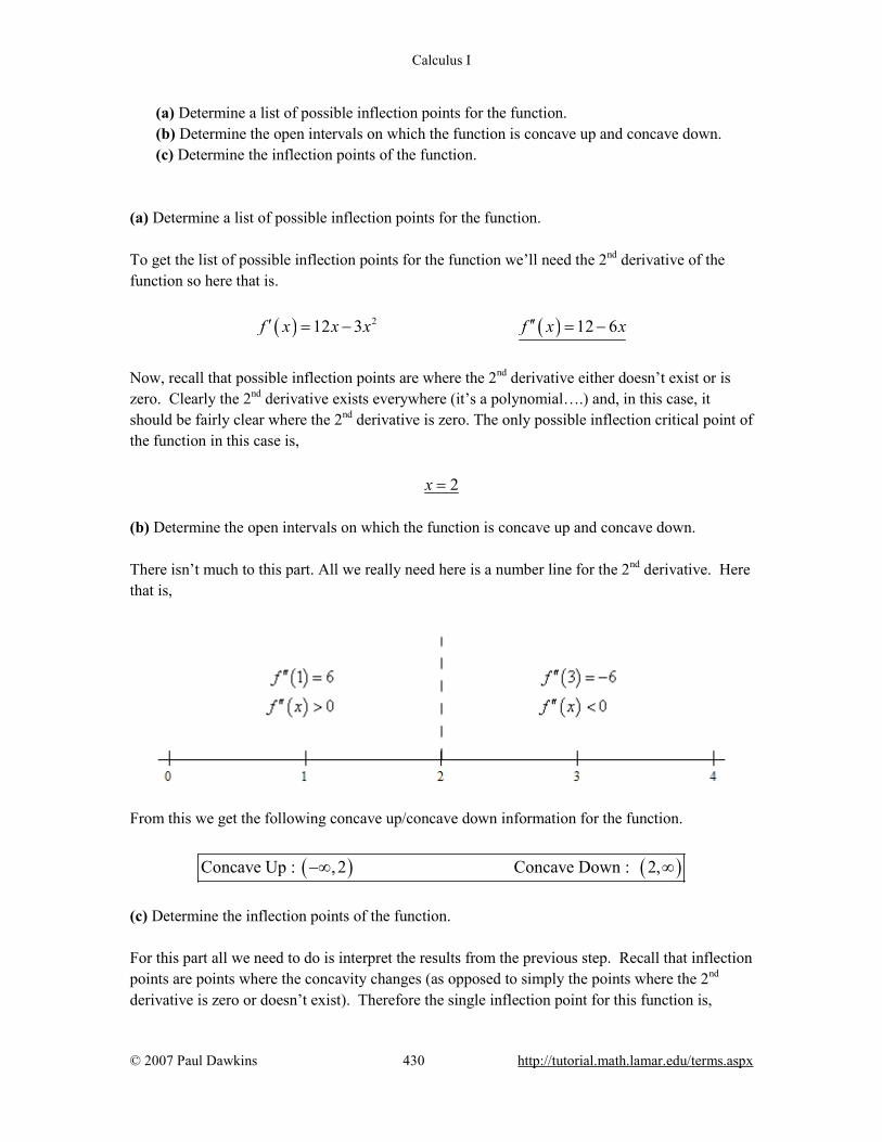
Calculus I
© 2007 Paul Dawkins 430 http://tutorial.math.lamar.edu/terms.aspx
(a) Determine a list of possible inflection points for the function. (b) Determine the open intervals on which the function is concave up and concave down. (c) Determine the inflection points of the function.
(a) Determine a list of possible inflection points for the function. To get the list of possible inflection points for the function we’ll need the 2nd derivative of the function so here that is.
( ) ( )212 3 12 6f x x x f x x′ ′′= − = −
Now, recall that possible inflection points are where the 2nd derivative either doesn’t exist or is zero. Clearly the 2nd derivative exists everywhere (it’s a polynomial….) and, in this case, it should be fairly clear where the 2nd derivative is zero. The only possible inflection critical point of the function in this case is, 2x =
(b) Determine the open intervals on which the function is concave up and concave down. There isn’t much to this part. All we really need here is a number line for the 2nd derivative. Here that is,
From this we get the following concave up/concave down information for the function.
( ) ( )Concave Up : , 2 Concave Down : 2,−∞ ∞ (c) Determine the inflection points of the function. For this part all we need to do is interpret the results from the previous step. Recall that inflection points are points where the concavity changes (as opposed to simply the points where the 2nd derivative is zero or doesn’t exist). Therefore the single inflection point for this function is,

Calculus I
© 2007 Paul Dawkins 431 http://tutorial.math.lamar.edu/terms.aspx
2x = 4. For ( ) 4 312 84 4g z z z z= − + + answer each of the following questions.
(a) Determine a list of possible inflection points for the function. (b) Determine the open intervals on which the function is concave up and concave down. (c) Determine the inflection points of the function.
(a) Determine a list of possible inflection points for the function. To get the list of possible inflection points for the function we’ll need the 2nd derivative of the function so here that is.
( ) ( ) ( )3 2 24 36 84 12 72 12 6g z z z g z z z z z′ ′′= − + = − = −
Now, recall that possible inflection points are where the 2nd derivative either doesn’t exist or is zero. Clearly the 2nd derivative exists everywhere (it’s a polynomial….) and, because we factored the 2nd derivative, it should be fairly clear where the 2nd derivative is zero. The possible inflection critical points of this function are, 0 & 6z z= =
(b) Determine the open intervals on which the function is concave up and concave down. There isn’t much to this part. All we really need here is a number line for the 2nd derivative. Here that is,
From this we get the following concave up/concave down information for the function.
( ) ( ) ( )Concave Up : ,0 & 6, Concave Down : 0,6−∞ ∞

Calculus I
© 2007 Paul Dawkins 432 http://tutorial.math.lamar.edu/terms.aspx
(c) Determine the inflection points of the function. For this part all we need to do is interpret the results from the previous step. Recall that inflection points are points where the concavity changes (as opposed to simply the points where the 2nd derivative is zero or doesn’t exist). Therefore the inflection points for this function are,
0 & 6z z= = 5. For ( ) 4 3 212 6 36 2h t t t t t= + + − + answer each of the following questions.
(a) Determine a list of possible inflection points for the function. (b) Determine the open intervals on which the function is concave up and concave down. (c) Determine the inflection points of the function.
(a) Determine a list of possible inflection points for the function. To get the list of possible inflection points for the function we’ll need the 2nd derivative of the function so here that is.
( ) ( ) ( )3 2 2 24 36 12 36 12 72 12 12 6 1h t t t t h t t t t t′ ′′= + + − = + + = + +
Now, recall that possible inflection points are where the 2nd derivative either doesn’t exist or is zero. Clearly the 2nd derivative exists everywhere (it’s a polynomial….). In this case the 2nd derivative doesn’t factor and so we’ll need to use the quadratic formula to determine where the 2nd derivative is zero. The possible inflection critical points of this function are,
3 2 2 5.8284, 0.1716t = − ± = − −
(b) Determine the open intervals on which the function is concave up and concave down. There isn’t much to this part. All we really need here is a number line for the 2nd derivative. Here that is,

Calculus I
© 2007 Paul Dawkins 433 http://tutorial.math.lamar.edu/terms.aspx
From this we get the following concave up/concave down information for the function.
( ) ( )( )
Concave Up : , 3 2 2 & 3 2 2,
Concave Down : 3 2 2, 3 2 2
−∞ − − − + ∞
− − − +
(c) Determine the inflection points of the function. For this part all we need to do is interpret the results from the previous step. Recall that inflection points are points where the concavity changes (as opposed to simply the points where the 2nd derivative is zero or doesn’t exist). Therefore the inflection points for this function are,
3 2 2 & 3 2 2t t= − − = − + 6. For ( ) ( )28 5 2 cos 3h w w w w= − + − on [ ]1, 2− answer each of the following questions.
(a) Determine a list of possible inflection points for the function. (b) Determine the open intervals on which the function is concave up and concave down. (c) Determine the inflection points of the function.
(a) Determine a list of possible inflection points for the function. To get the list of possible inflection points for the function we’ll need the 2nd derivative of the function so here that is.
( ) ( ) ( ) ( )5 4 3sin 3 4 9cos 3h w w w h w w′ ′′= − + + = +
Now, recall that possible inflection points are where the 2nd derivative either doesn’t exist or is zero. Clearly the 2nd derivative exists everywhere (the cosine function exists everywhere…) and so all we need to do is set the 2nd derivative equal to zero and solve. We’re not going to show all
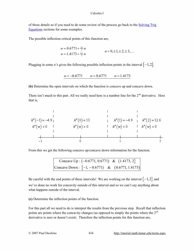
Calculus I
© 2007 Paul Dawkins 434 http://tutorial.math.lamar.edu/terms.aspx
of those details so if you need to do some review of the process go back to the Solving Trig Equations sections for some examples. The possible inflection critical points of this function are,
23
23
0.67710, 1, 2, 3,
1.4173w n
nw n
π
π
= += ± ± ±
= +…
Plugging in some n’s gives the following possible inflection points in the interval [ ]1, 2− .
0.6771 0.6771 1.4173w w w= − = = (b) Determine the open intervals on which the function is concave up and concave down. There isn’t much to this part. All we really need here is a number line for the 2nd derivative. Here that is,
From this we get the following concave up/concave down information for the function.
( ) ( ][ ) ( )
Concave Up : 0.6771, 0.6771 & 1.4173, 2
Concave Down : 1, 0.6771 & 0.6771, 1.4173
−
− −
Be careful with the end points of these intervals! We are working on the interval [ ]1, 2− and
we’ve done no work for concavity outside of this interval and so we can’t say anything about what happens outside of the interval. (c) Determine the inflection points of the function. For this part all we need to do is interpret the results from the previous step. Recall that inflection points are points where the concavity changes (as opposed to simply the points where the 2nd derivative is zero or doesn’t exist). Therefore the inflection points for this function are,
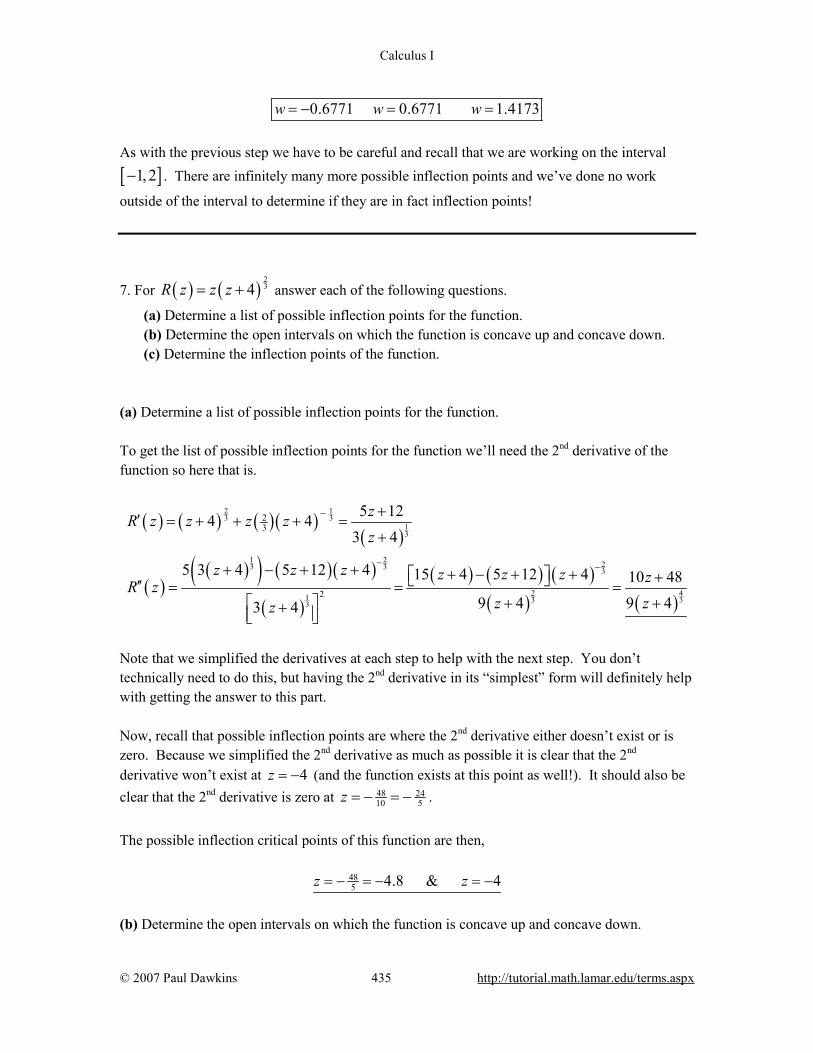
Calculus I
© 2007 Paul Dawkins 435 http://tutorial.math.lamar.edu/terms.aspx
0.6771 0.6771 1.4173w w w= − = =
As with the previous step we have to be careful and recall that we are working on the interval
[ ]1, 2− . There are infinitely many more possible inflection points and we’ve done no work
outside of the interval to determine if they are in fact inflection points!
7. For ( ) ( )234R z z z= + answer each of the following questions.
(a) Determine a list of possible inflection points for the function. (b) Determine the open intervals on which the function is concave up and concave down. (c) Determine the inflection points of the function.
(a) Determine a list of possible inflection points for the function. To get the list of possible inflection points for the function we’ll need the 2nd derivative of the function so here that is.
( ) ( ) ( ) ( )( )
( )( )( ) ( )( )
( )
( ) ( ) ( )( ) ( )
2 13 3
13
1 2 23 3 3
2 41 3 33
23
2
5 124 43 4
5 3 4 5 12 4 15 4 5 12 4 10 489 4 9 43 4
zR z z z zz
z z z z z z zR zz zz
− −
− +′ = + + + =+
+ − + + + − + + + ′′ = = = + ++
Note that we simplified the derivatives at each step to help with the next step. You don’t technically need to do this, but having the 2nd derivative in its “simplest” form will definitely help with getting the answer to this part. Now, recall that possible inflection points are where the 2nd derivative either doesn’t exist or is zero. Because we simplified the 2nd derivative as much as possible it is clear that the 2nd derivative won’t exist at 4z = − (and the function exists at this point as well!). It should also be clear that the 2nd derivative is zero at 48 24
10 5z = − = − . The possible inflection critical points of this function are then, 48
5 4.8 & 4z z= − = − = −
(b) Determine the open intervals on which the function is concave up and concave down.
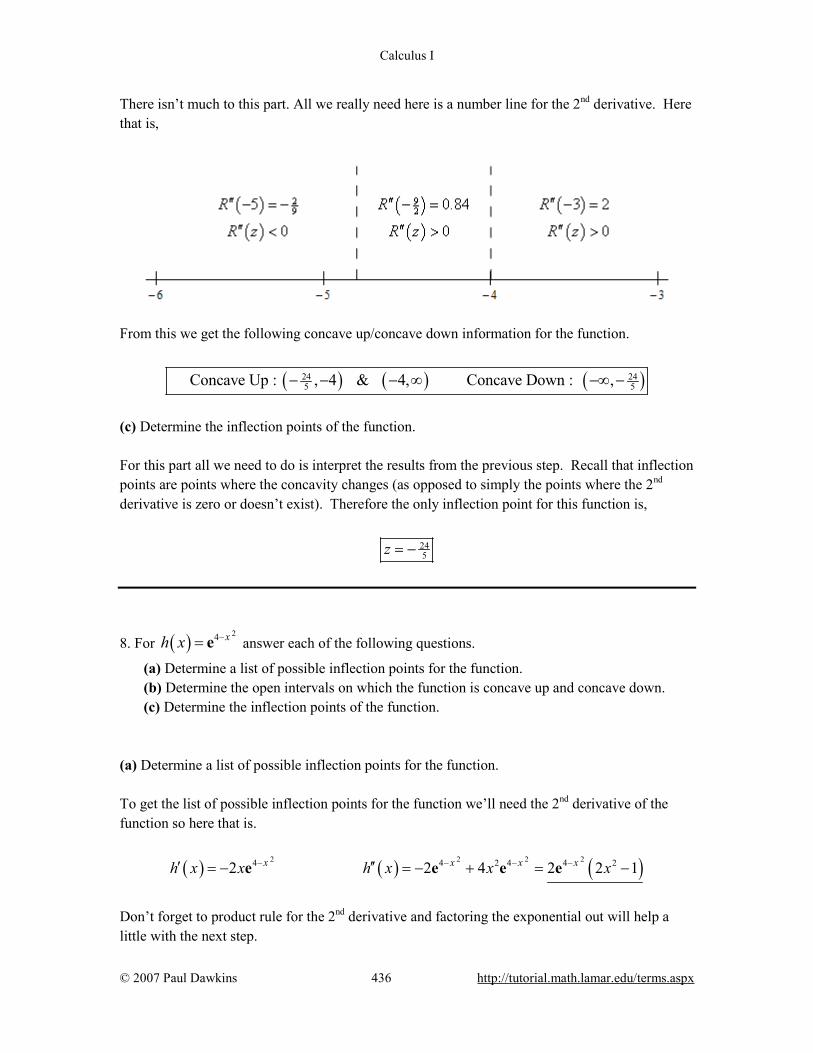
Calculus I
© 2007 Paul Dawkins 436 http://tutorial.math.lamar.edu/terms.aspx
There isn’t much to this part. All we really need here is a number line for the 2nd derivative. Here that is,
From this we get the following concave up/concave down information for the function.
( ) ( ) ( )24 245 5Concave Up : , 4 & 4, Concave Down : ,− − − ∞ −∞ −
(c) Determine the inflection points of the function. For this part all we need to do is interpret the results from the previous step. Recall that inflection points are points where the concavity changes (as opposed to simply the points where the 2nd derivative is zero or doesn’t exist). Therefore the only inflection point for this function is,
245z = −
8. For ( ) 24 xh x −= e answer each of the following questions.
(a) Determine a list of possible inflection points for the function. (b) Determine the open intervals on which the function is concave up and concave down. (c) Determine the inflection points of the function.
(a) Determine a list of possible inflection points for the function. To get the list of possible inflection points for the function we’ll need the 2nd derivative of the function so here that is.
( ) ( ) ( )2 2 2 24 4 2 4 4 22 2 4 2 2 1x x x xh x x h x x x− − − −′ ′′= − = − + = −e e e e
Don’t forget to product rule for the 2nd derivative and factoring the exponential out will help a little with the next step.

Calculus I
© 2007 Paul Dawkins 437 http://tutorial.math.lamar.edu/terms.aspx
Now, recall that possible inflection points are where the 2nd derivative either doesn’t exist or is zero. It should be fairly clear that the 2nd derivative exists everywhere (it is a product of two functions that exist everywhere…). We also know that exponentials are never zero and so the 2nd derivative will be zero at the solutions to 22 1 0x − = The possible inflection critical points of this function are then, 1
20.7071x = ± = ±
(b) Determine the open intervals on which the function is concave up and concave down. There isn’t much to this part. All we really need here is a number line for the 2nd derivative. Here that is,
From this we get the following concave up/concave down information for the function.
( ) ( ) ( )1 1 1 12 2 2 2
Concave Up : , & , Concave Down : ,−∞ − ∞ −
(c) Determine the inflection points of the function. For this part all we need to do is interpret the results from the previous step. Recall that inflection points are points where the concavity changes (as opposed to simply the points where the 2nd derivative is zero or doesn’t exist). Therefore the only inflection point for this function is,
1 12 2
0.7071 0.7071x x= − = − = =
9. For ( ) 5 45 8g t t t= − + answer each of the following questions.
(a) Identify the critical points of the function. (b) Determine the open intervals on which the function increases and decreases.

Calculus I
© 2007 Paul Dawkins 438 http://tutorial.math.lamar.edu/terms.aspx
(c) Classify the critical points as relative maximums, relative minimums or neither. (d) Determine the open intervals on which the function is concave up and concave down. (e) Determine the inflection points of the function. (f) Use the information from steps (a) – (e) to sketch the graph of the function.
(a) Identify the critical points of the function. The parts to this problem (with the exception of the last part) are just like the basic increasing/decreasing problems from the previous section and the basic concavity problems from earlier in this section. Because of that we will not be putting in quite as much detail here. If you are still unsure how to work the parts of this problem you should go back and work a few of the basic problems from the previous section and/or earlier in this section before proceeding. We will need the 1st derivative to start things off.
( ) ( )4 3 35 20 5 4g t t t t t′ = − = −
From the 1st derivative we can see that the critical points of this function are then, 0 & 4t t= =
(b) Determine the open intervals on which the function increases and decreases. To answer this part all we need is the number line for the 1st derivative.
From this we get the following increasing/decreasing information for the function.
( ) ( ) ( )Increasing : ,0 & 4, Decreasing : 0, 4−∞ ∞ (c) Classify the critical points as relative maximums, relative minimums or neither. From the number line in the previous step we get the following classifications of the critical points.
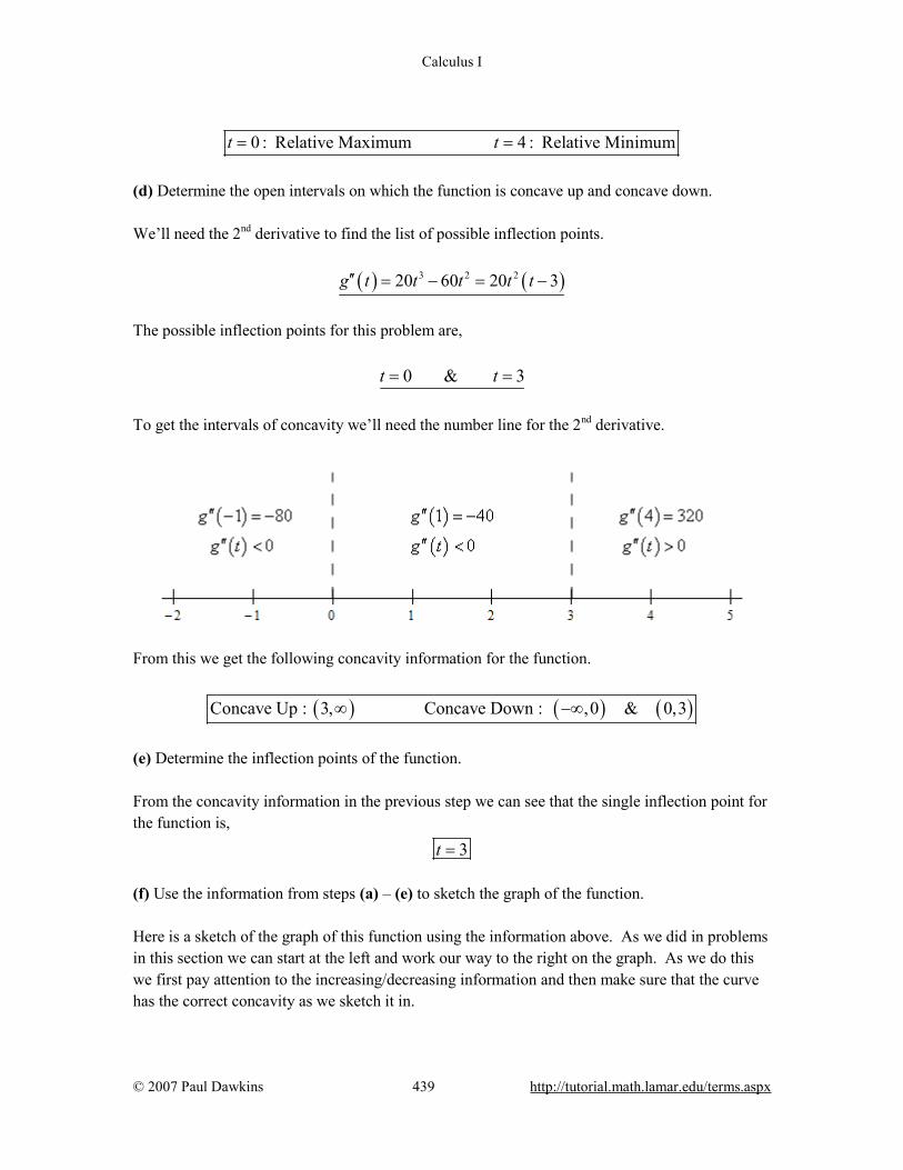
Calculus I
© 2007 Paul Dawkins 439 http://tutorial.math.lamar.edu/terms.aspx
0 : Relative Maximum 4 : Relative Minimumt t= =
(d) Determine the open intervals on which the function is concave up and concave down. We’ll need the 2nd derivative to find the list of possible inflection points. ( ) ( )3 2 220 60 20 3g t t t t t′′ = − = − The possible inflection points for this problem are, 0 & 3t t= = To get the intervals of concavity we’ll need the number line for the 2nd derivative.
From this we get the following concavity information for the function.
( ) ( ) ( )Concave Up : 3, Concave Down : ,0 & 0,3∞ −∞ (e) Determine the inflection points of the function. From the concavity information in the previous step we can see that the single inflection point for the function is,
3t = (f) Use the information from steps (a) – (e) to sketch the graph of the function. Here is a sketch of the graph of this function using the information above. As we did in problems in this section we can start at the left and work our way to the right on the graph. As we do this we first pay attention to the increasing/decreasing information and then make sure that the curve has the correct concavity as we sketch it in.

Calculus I
© 2007 Paul Dawkins 440 http://tutorial.math.lamar.edu/terms.aspx
Note that because we used a computer to generate the sketch it is possible that your sketch won’t be quite the same. It should however, have the same points listed on the graph above, the same basic increasing/decreasing nature and the same basic concavity. 10. For ( ) 3 45 8f x x x= − − answer each of the following questions.
(a) Identify the critical points of the function. (b) Determine the open intervals on which the function increases and decreases. (c) Classify the critical points as relative maximums, relative minimums or neither. (d) Determine the open intervals on which the function is concave up and concave down. (e) Determine the inflection points of the function. (f) Use the information from steps (a) – (e) to sketch the graph of the function.
(a) Identify the critical points of the function. The parts to this problem (with the exception of the last part) are just like the basic increasing/decreasing problems from the previous section and the basic concavity problems from earlier in this section. Because of that we will not be putting in quite as much detail here. If you are still unsure how to work the parts of this problem you should go back and work a few of the basic problems from the previous section and/or earlier in this section before proceeding. We will need the 1st derivative to start things off.
( ) ( )2 3 224 4 4 6f x x x x x′ = − − = − +
From the 1st derivative we can see that the critical points of this function are then,

Calculus I
© 2007 Paul Dawkins 441 http://tutorial.math.lamar.edu/terms.aspx
6 & 0x x= − =
(b) Determine the open intervals on which the function increases and decreases. To answer this part all we need is the number line for the 1st derivative.
From this we get the following increasing/decreasing information for the function.
( ) ( ) ( )Increasing : , 6 Decreasing : 6,0 & 0,−∞ − − ∞ (c) Classify the critical points as relative maximums, relative minimums or neither. From the number line in the previous step we get the following classifications of the critical points.
6 : Relative Maximum 0 : Neitherx x= − =
(d) Determine the open intervals on which the function is concave up and concave down. We’ll need the 2nd derivative to find the list of possible inflection points. ( ) ( )248 12 12 4f x x x x x′′ = − − = − + The possible inflection points for this function are, 4 & 0x x= − = To get the intervals of concavity we’ll need the number line for the 2nd derivative.
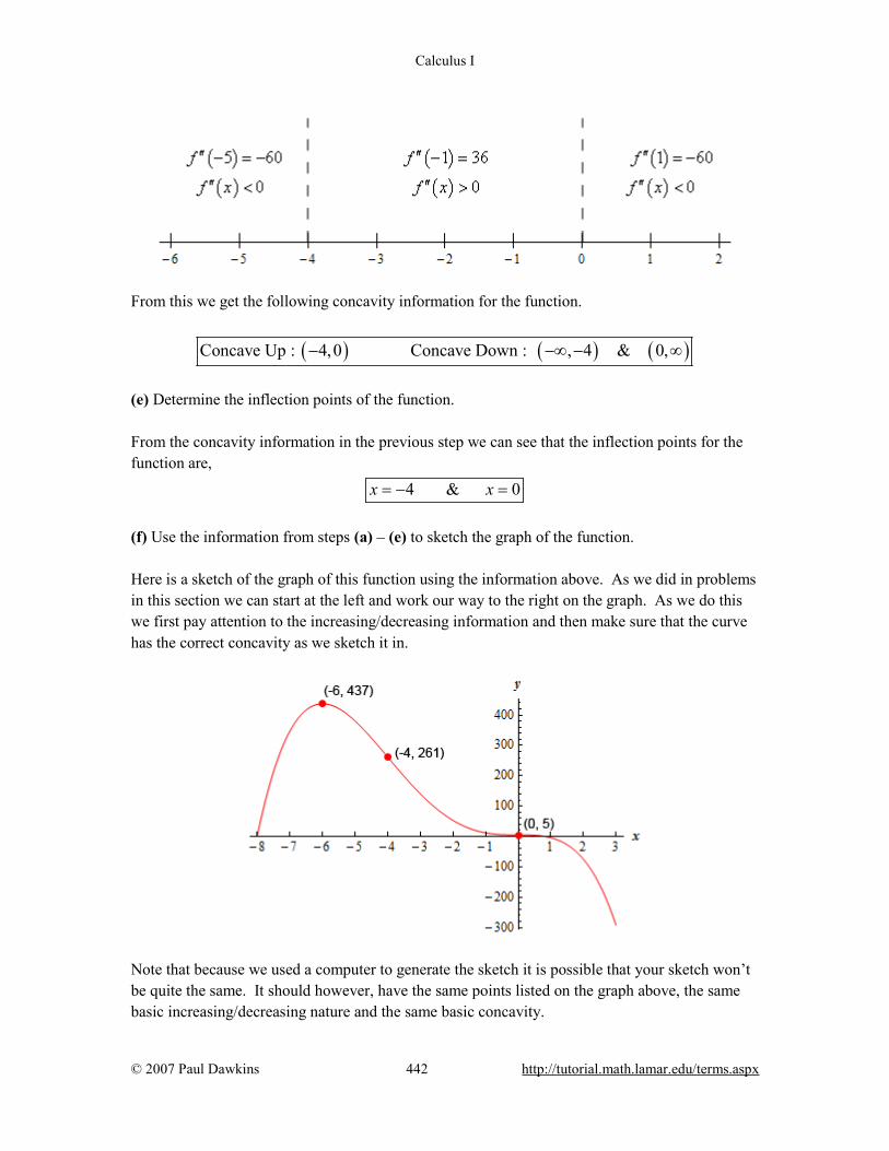
Calculus I
© 2007 Paul Dawkins 442 http://tutorial.math.lamar.edu/terms.aspx
From this we get the following concavity information for the function.
( ) ( ) ( )Concave Up : 4,0 Concave Down : , 4 & 0,− −∞ − ∞ (e) Determine the inflection points of the function. From the concavity information in the previous step we can see that the inflection points for the function are,
4 & 0x x= − = (f) Use the information from steps (a) – (e) to sketch the graph of the function. Here is a sketch of the graph of this function using the information above. As we did in problems in this section we can start at the left and work our way to the right on the graph. As we do this we first pay attention to the increasing/decreasing information and then make sure that the curve has the correct concavity as we sketch it in.
Note that because we used a computer to generate the sketch it is possible that your sketch won’t be quite the same. It should however, have the same points listed on the graph above, the same basic increasing/decreasing nature and the same basic concavity.

Calculus I
© 2007 Paul Dawkins 443 http://tutorial.math.lamar.edu/terms.aspx
11. For ( ) 4 3 22 12h z z z z= − − answer each of the following questions.
(a) Identify the critical points of the function. (b) Determine the open intervals on which the function increases and decreases. (c) Classify the critical points as relative maximums, relative minimums or neither. (d) Determine the open intervals on which the function is concave up and concave down. (e) Determine the inflection points of the function. (f) Use the information from steps (a) – (e) to sketch the graph of the function.
(a) Identify the critical points of the function. The parts to this problem (with the exception of the last part) are just like the basic increasing/decreasing problems from the previous section and the basic concavity problems from earlier in this section. Because of that we will not be putting in quite as much detail here. If you are still unsure how to work the parts of this problem you should go back and work a few of the basic problems from the previous section and/or earlier in this section before proceeding. We will need the 1st derivative to start things off.
( ) ( )3 2 24 6 24 2 2 3 12h z z z z z z z′ = − − = − −
From the 1st derivative we can see that the critical points of this function are then,
3 10540 & 1.8117, 3.3117x x ±= = = −
(b) Determine the open intervals on which the function increases and decreases. To answer this part all we need is the number line for the 1st derivative.
From this we get the following increasing/decreasing information for the function.

Calculus I
© 2007 Paul Dawkins 444 http://tutorial.math.lamar.edu/terms.aspx
( ) ( ) ( ) ( )3 105 3 105 3 105 3 1054 4 4 4Increasing : ,0 & , Decreasing : , & 0,− + − +∞ −∞
(c) Classify the critical points as relative maximums, relative minimums or neither. From the number line in the previous step we get the following classifications of the critical points.
3 105
4
3 1054
: Relative Minimum 0 : Relative Maximum
: Relative Minimum
z z
z
−
+
= =
=
(d) Determine the open intervals on which the function is concave up and concave down. We’ll need the 2nd derivative to find the list of possible inflection points. ( ) ( ) ( )212 12 24 12 2 1h z z z z z′′ = − − = − + The possible inflection points for this function are, 1 & 2z z= − = To get the intervals of concavity we’ll need the number line for the 2nd derivative.
From this we get the following concavity information for the function.
( ) ( ) ( )Concave Up : , 1 & 2, Concave Down : 1, 2−∞ − ∞ − (e) Determine the inflection points of the function. From the concavity information in the previous step we can see that the inflection points for the function are,

Calculus I
© 2007 Paul Dawkins 445 http://tutorial.math.lamar.edu/terms.aspx
1 & 2z z= − = (f) Use the information from steps (a) – (e) to sketch the graph of the function. Here is a sketch of the graph of this function using the information above. As we did in problems in this section we can start at the left and work our way to the right on the graph. As we do this we first pay attention to the increasing/decreasing information and then make sure that the curve has the correct concavity as we sketch it in.
Note that because we used a computer to generate the sketch it is possible that your sketch won’t be quite the same. It should however, have the same points listed on the graph above, the same basic increasing/decreasing nature and the same basic concavity. 12. For ( ) ( )23 8sin tQ t t= − on [ ]7,4− answer each of the following questions.
(a) Identify the critical points of the function. (b) Determine the open intervals on which the function increases and decreases. (c) Classify the critical points as relative maximums, relative minimums or neither. (d) Determine the open intervals on which the function is concave up and concave down. (e) Determine the inflection points of the function. (f) Use the information from steps (a) – (e) to sketch the graph of the function.
(a) Identify the critical points of the function. The parts to this problem (with the exception of the last part) are just like the basic increasing/decreasing problems from the previous section and the basic concavity problems from
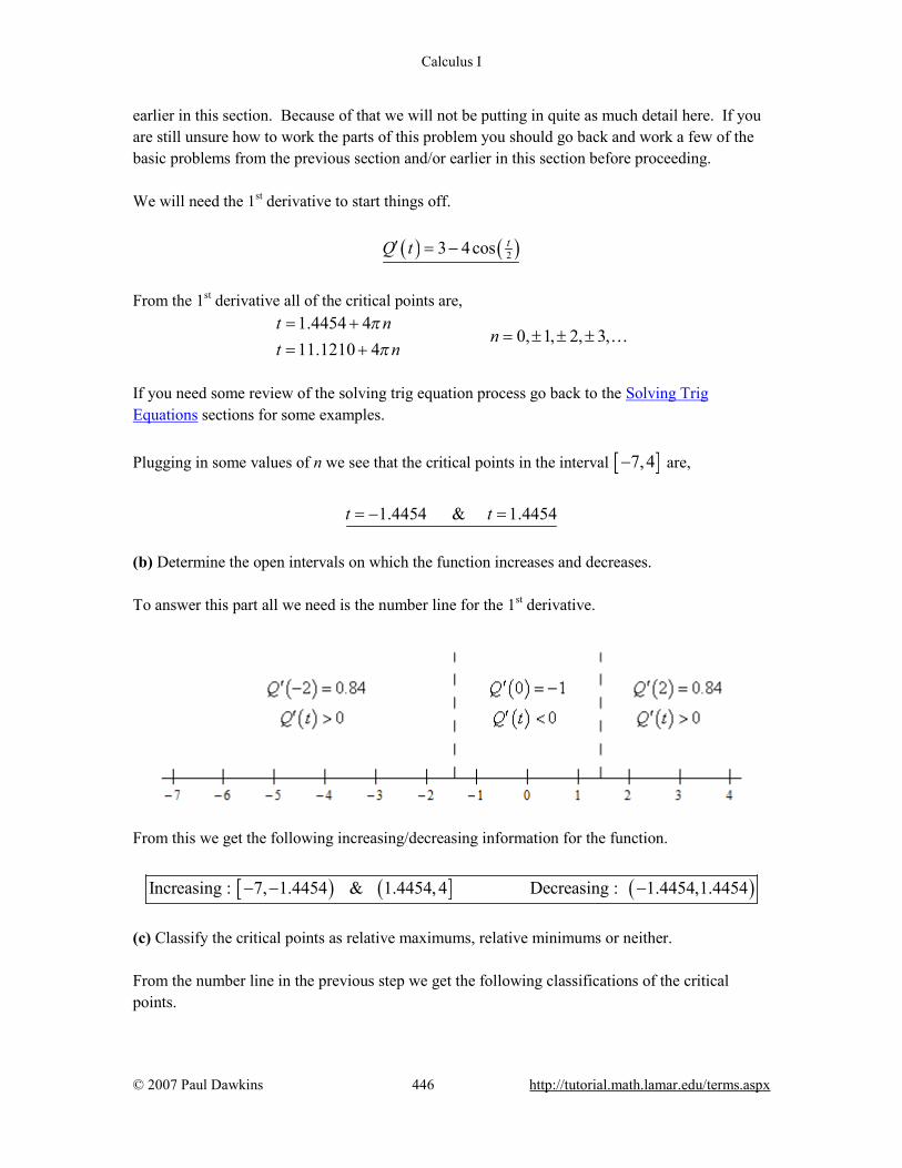
Calculus I
© 2007 Paul Dawkins 446 http://tutorial.math.lamar.edu/terms.aspx
earlier in this section. Because of that we will not be putting in quite as much detail here. If you are still unsure how to work the parts of this problem you should go back and work a few of the basic problems from the previous section and/or earlier in this section before proceeding. We will need the 1st derivative to start things off.
( ) ( )23 4cos tQ t′ = −
From the 1st derivative all of the critical points are,
1.4454 4
0, 1, 2, 3,11.1210 4
t nn
t nπ
π= +
= ± ± ±= +
…
If you need some review of the solving trig equation process go back to the Solving Trig Equations sections for some examples. Plugging in some values of n we see that the critical points in the interval [ ]7,4− are,
1.4454 & 1.4454t t= − =
(b) Determine the open intervals on which the function increases and decreases. To answer this part all we need is the number line for the 1st derivative.
From this we get the following increasing/decreasing information for the function.
[ ) ( ] ( )Increasing : 7, 1.4454 & 1.4454, 4 Decreasing : 1.4454,1.4454− − − (c) Classify the critical points as relative maximums, relative minimums or neither. From the number line in the previous step we get the following classifications of the critical points.
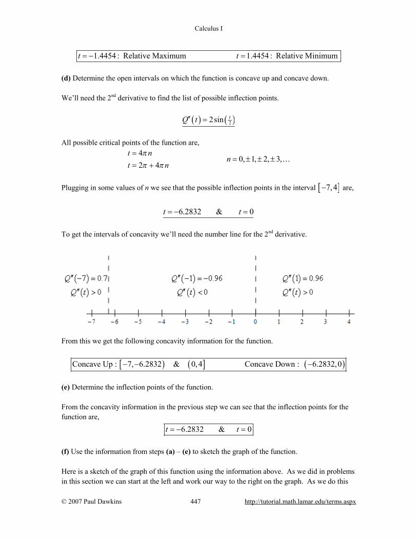
Calculus I
© 2007 Paul Dawkins 447 http://tutorial.math.lamar.edu/terms.aspx
1.4454 : Relative Maximum 1.4454 : Relative Minimumt t= − =
(d) Determine the open intervals on which the function is concave up and concave down. We’ll need the 2nd derivative to find the list of possible inflection points. ( ) ( )22sin tQ t′′ = All possible critical points of the function are,
4
0, 1, 2, 3,2 4
t nn
t nππ π
== ± ± ±
= +…
Plugging in some values of n we see that the possible inflection points in the interval [ ]7,4− are,
6.2832 & 0t t= − = To get the intervals of concavity we’ll need the number line for the 2nd derivative.
From this we get the following concavity information for the function.
[ ) ( ] ( )Concave Up : 7, 6.2832 & 0,4 Concave Down : 6.2832,0− − − (e) Determine the inflection points of the function. From the concavity information in the previous step we can see that the inflection points for the function are,
6.2832 & 0t t= − = (f) Use the information from steps (a) – (e) to sketch the graph of the function. Here is a sketch of the graph of this function using the information above. As we did in problems in this section we can start at the left and work our way to the right on the graph. As we do this
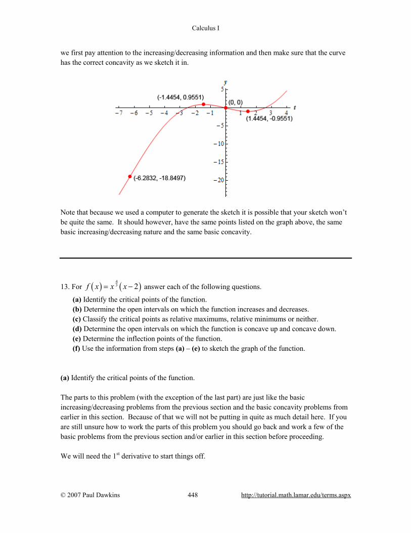
Calculus I
© 2007 Paul Dawkins 448 http://tutorial.math.lamar.edu/terms.aspx
we first pay attention to the increasing/decreasing information and then make sure that the curve has the correct concavity as we sketch it in.
Note that because we used a computer to generate the sketch it is possible that your sketch won’t be quite the same. It should however, have the same points listed on the graph above, the same basic increasing/decreasing nature and the same basic concavity.
13. For ( ) ( )43 2f x x x= − answer each of the following questions.
(a) Identify the critical points of the function. (b) Determine the open intervals on which the function increases and decreases. (c) Classify the critical points as relative maximums, relative minimums or neither. (d) Determine the open intervals on which the function is concave up and concave down. (e) Determine the inflection points of the function. (f) Use the information from steps (a) – (e) to sketch the graph of the function.
(a) Identify the critical points of the function. The parts to this problem (with the exception of the last part) are just like the basic increasing/decreasing problems from the previous section and the basic concavity problems from earlier in this section. Because of that we will not be putting in quite as much detail here. If you are still unsure how to work the parts of this problem you should go back and work a few of the basic problems from the previous section and/or earlier in this section before proceeding. We will need the 1st derivative to start things off.

Calculus I
© 2007 Paul Dawkins 449 http://tutorial.math.lamar.edu/terms.aspx
( ) ( ) ( )7 4 4 1 13 3 3 3 37 8 1
3 3 32 7 8f x x x f x x x x x′= − → = − = −
Note that by factoring the 13x out we made it a little easier to quickly see that the critical points
are, 8
70 & 1.1429x x= = =
(b) Determine the open intervals on which the function increases and decreases. To answer this part all we need is the number line for the 1st derivative.
From this we get the following increasing/decreasing information for the function.
( ) ( ) ( )8 87 7Increasing : ,0 & , Decreasing : 0,−∞ ∞
(c) Classify the critical points as relative maximums, relative minimums or neither. From the number line in the previous step we get the following classifications of the critical points.
870 : Relative Maximum : Relative Minimumx x= =
(d) Determine the open intervals on which the function is concave up and concave down. We’ll need the 2nd derivative to find the list of possible inflection points.
( )1 23 3
23
28 89 9
28 89xf x x xx
− −′′ = − =
The possible inflection points for this function are,
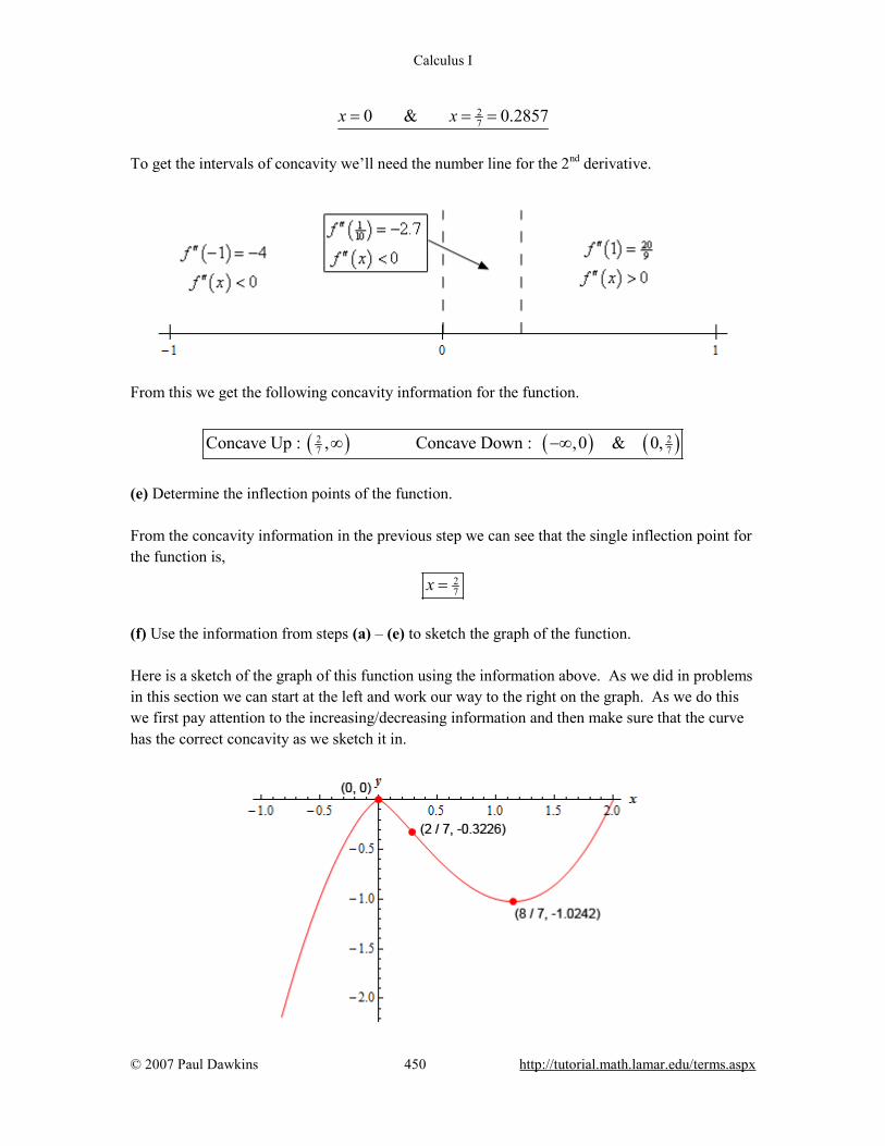
Calculus I
© 2007 Paul Dawkins 450 http://tutorial.math.lamar.edu/terms.aspx
270 & 0.2857x x= = =
To get the intervals of concavity we’ll need the number line for the 2nd derivative.
From this we get the following concavity information for the function.
( ) ( ) ( )2 27 7Concave Up : , Concave Down : ,0 & 0,∞ −∞
(e) Determine the inflection points of the function. From the concavity information in the previous step we can see that the single inflection point for the function is,
27x =
(f) Use the information from steps (a) – (e) to sketch the graph of the function. Here is a sketch of the graph of this function using the information above. As we did in problems in this section we can start at the left and work our way to the right on the graph. As we do this we first pay attention to the increasing/decreasing information and then make sure that the curve has the correct concavity as we sketch it in.
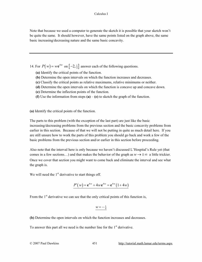
Calculus I
© 2007 Paul Dawkins 451 http://tutorial.math.lamar.edu/terms.aspx
Note that because we used a computer to generate the sketch it is possible that your sketch won’t be quite the same. It should however, have the same points listed on the graph above, the same basic increasing/decreasing nature and the same basic concavity. 14. For ( ) 4wP w w= e on [ ]1
42,− answer each of the following questions.
(a) Identify the critical points of the function. (b) Determine the open intervals on which the function increases and decreases. (c) Classify the critical points as relative maximums, relative minimums or neither. (d) Determine the open intervals on which the function is concave up and concave down. (e) Determine the inflection points of the function. (f) Use the information from steps (a) – (e) to sketch the graph of the function.
(a) Identify the critical points of the function. The parts to this problem (with the exception of the last part) are just like the basic increasing/decreasing problems from the previous section and the basic concavity problems from earlier in this section. Because of that we will not be putting in quite as much detail here. If you are still unsure how to work the parts of this problem you should go back and work a few of the basic problems from the previous section and/or earlier in this section before proceeding. Also note that the interval here is only because we haven’t discussed L’Hospital’s Rule yet (that comes in a few sections…) and that makes the behavior of the graph as w → ± ∞ a little trickier. Once we cover that section you might want to come back and eliminate the interval and see what the graph is. We will need the 1st derivative to start things off.
( ) ( )4 4 44 1 4w w wP w w w′ = + = +e e e
From the 1st derivative we can see that the only critical points of this function is, 1
4w = −
(b) Determine the open intervals on which the function increases and decreases. To answer this part all we need is the number line for the 1st derivative.
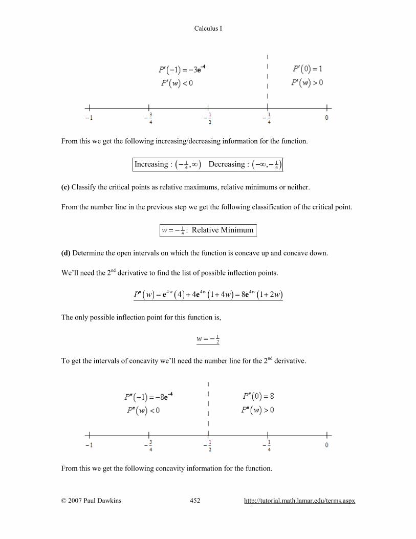
Calculus I
© 2007 Paul Dawkins 452 http://tutorial.math.lamar.edu/terms.aspx
From this we get the following increasing/decreasing information for the function.
( ) ( )1 14 4Increasing : , Decreasing : ,− ∞ −∞ −
(c) Classify the critical points as relative maximums, relative minimums or neither. From the number line in the previous step we get the following classification of the critical point.
14 : Relative Minimumw = −
(d) Determine the open intervals on which the function is concave up and concave down. We’ll need the 2nd derivative to find the list of possible inflection points. ( ) ( ) ( ) ( )4 4 44 4 1 4 8 1 2w w wP w w w′′ = + + = +e e e The only possible inflection point for this function is, 1
2w = − To get the intervals of concavity we’ll need the number line for the 2nd derivative.
From this we get the following concavity information for the function.

Calculus I
© 2007 Paul Dawkins 453 http://tutorial.math.lamar.edu/terms.aspx
( ) ( )1 12 2Concave Up : , Concave Down : ,− ∞ −∞ −
(e) Determine the inflection points of the function. From the concavity information in the previous step we can see that the single inflection point for the function is,
12w = −
(f) Use the information from steps (a) – (e) to sketch the graph of the function. Here is a sketch of the graph of this function using the information above. As we did in problems in this section we can start at the left and work our way to the right on the graph. As we do this we first pay attention to the increasing/decreasing information and then make sure that the curve has the correct concavity as we sketch it in.
Note that because we used a computer to generate the sketch it is possible that your sketch won’t be quite the same. It should however, have the same points listed on the graph above, the same basic increasing/decreasing nature and the same basic concavity. 15. Determine the minimum degree of a polynomial that has exactly one inflection point. Hint : What is the simplest possible form of the 2nd derivative that we can have that will guarantee that we have a single inflection point? Step 1

Calculus I
© 2007 Paul Dawkins 454 http://tutorial.math.lamar.edu/terms.aspx
First, let’s suppose that the single inflection point occurs at x a= for some number a. The value of a is not important, this only allows us to discuss the problem. Now, if we start with a polynomial, call it ( )p x , then the 2nd derivative must also be a
polynomial and we have to have ( ) 0p a′′ = . In addition we know that the 2nd derivative must
change signs at x a= . The simplest polynomial that we can have that will do this is,
( )p x x a′′ = −
This clearly has ( ) 0p a′′ = and it will change sign at x a= . Note as well that we don’t really
care which side is concave up and which side is concave down. We only care that the 2nd derivative changes sign at x a= as it does here. Hint : We saw how to “undo” differentiation in the practice problems in the previous section. Here we simply need to do that twice and note that we don’t actually have to undo the derivatives here, just think about what they would have to look like. Step 2 Okay, saw how to “undo” differentiation in the practice problems of the previous section. We don’t actually need to do that here, but we do need to think about what undoing differentiation will give here. The 2nd derivative is a 1st degree polynomial and that means the 1st derivative had to be a 2nd degree polynomial. This should make sense to you if you understand how differentiation works. We know that we have to differentiate the 1st derivative to get the 2nd derivative. Therefore because the highest power of x in the 2nd derivative is 1 and we know that differentiation lowers the power by 1 the highest power of x in the 1st derivative must have been 2. Okay, we’ve figured out that the 1st derivative must have been a 2nd degree polynomial. This in turn means that the original function must have been a 3rd degree polynomial Again, differentiation lowers the power of x by 1 and if the highest power of x in the 1st derivative is 2 then the highest power of x in the original function must have been 3. So, the minimum degree of a polynomial that has exactly one inflection point must be three (i.e. a cubic polynomial).
Calculus I
© 2007 Paul Dawkins 455 http://tutorial.math.lamar.edu/terms.aspx
Note that we can have higher degree polynomials with exactly one inflection point. This is simply the minimal degree that will give exactly one inflection point. 16. Suppose that we know that ( )f x is a polynomial with critical points 1x = − , 2x = and
6x = . If we also know that the 2nd derivative is ( ) 23 14 4f x x x′′ = + − . If possible, classify
each of the critical points as relative minimums, relative maximums. If it is not possible to classify the critical points clearly explain why they cannot be classified. Hint : We do NOT need the 1st derivative to answer this question. We are in the 2nd derivative section and we did see a way in the notes on how to use the 2nd derivative (which we have nicely been given…) to classify most critical points. Solution This problem is not as difficult as many students originally make it out to be. We’ve been given the 2nd derivative and we saw how the 2nd derivative test can be used to classify most critical points so let’s use that. First, we should note that because we have been told that ( )f x is a polynomial it should be
fairly clear that, regardless of what the 1st derivative actually is, we should have, ( ) ( ) ( )1 0 2 0 6 0f f f′ ′ ′− = = = What this means is that we can use the 2nd derivative test as it only works for these kinds of critical points. All we need to do then is plug the critical points into the 2nd derivative and use the 2nd derivative test to classify the critical points.
( )( )( )
1 21 0 Relative Maximum
2 12 0 Relative Minimum
6 28 0 Relative Maximum
f
f
f
′′ − = − <
′′ = >
′′ = − <
So, in this case it was possible to classify all of the given critical points. Recall that if the 2nd derivative had been zero for any of them we would not have been able to classify that critical point without the 1st derivative which we don’t have for this case.
Calculus I
© 2007 Paul Dawkins 456 http://tutorial.math.lamar.edu/terms.aspx
The Mean Value Theorem 1. Determine all the number(s) c which satisfy the conclusion of Rolle’s Theorem for
( ) 2 2 8f x x x= − − on [ ]1,3− .
Solution The first thing we should do is actually verify that Rolle’s Theorem can be used here. The function is a polynomial which is continuous and differentiable everywhere and so will be continuous on [ ]1,3− and differentiable on ( )1,3− .
Next, a couple of quick function evaluations shows that ( ) ( )1 3 5f f− = = − .
Therefore, the conditions for Rolle’s Theorem are met and so we can actually do the problem. Note that this may seem to be a little silly to check the conditions but it is a really good idea to get into the habit of doing this stuff. Since we are in this section it is pretty clear that the conditions will be met or we wouldn’t be asking the problem. However, once we get out of this section and you want to use the Theorem the conditions may not be met. If you are in the habit of not checking you could inadvertently use the Theorem on a problem that can’t be used and then get an incorrect answer. Now that we know that Rolle’s Theorem can be used there really isn’t much to do. All we need to do is take the derivative, ( ) 2 2f x x′ = − and then solve ( ) 0f c′ = .
2 2 0 1c c− = ⇒ = So, we found a single value and it is in the interval so the value we want is,
1c =

Calculus I
© 2007 Paul Dawkins 457 http://tutorial.math.lamar.edu/terms.aspx
2. Determine all the number(s) c which satisfy the conclusion of Rolle’s Theorem for
( ) 2 32g t t t t= − − on [ ]2,1− .
Solution The first thing we should do is actually verify that Rolle’s Theorem can be used here. The function is a polynomial which is continuous and differentiable everywhere and so will be continuous on [ ]2,1− and differentiable on ( )2,1− .
Next, a couple of quick function evaluations shows that ( ) ( )2 1 0g g− = = .
Therefore, the conditions for Rolle’s Theorem are met and so we can actually do the problem. Note that this may seem to be a little silly to check the conditions but it is a really good idea to get into the habit of doing this stuff. Since we are in this section it is pretty clear that the conditions will be met or we wouldn’t be asking the problem. However, once we get out of this section and you want to use the Theorem the conditions may not be met. If you are in the habit of not checking you could inadvertently use the Theorem on a problem that can’t be used and then get an incorrect answer. Now that we know that Rolle’s Theorem can be used there really isn’t much to do. All we need to do is take the derivative, ( ) 22 2 3g t t t′ = − − and then solve ( ) 0g c′ = .
2 1 733 2 2 0 1.2153, 0.5486c c c ±
−− − + = ⇒ = = − So, we found two values and, in this case, they are both in the interval so the values we want are,
1 73 1.2153, 0.5486c ±
−= = − 3. Determine all the number(s) c which satisfy the conclusion of Mean Value Theorem for
( ) 3 24 8 7 2h z z z z= − + − on [ ]2,5 .
Solution The first thing we should do is actually verify that the Mean Value Theorem can be used here.
Calculus I
© 2007 Paul Dawkins 458 http://tutorial.math.lamar.edu/terms.aspx
The function is a polynomial which is continuous and differentiable everywhere and so will be continuous on [ ]2,5 and differentiable on ( )2,5 .
Therefore, the conditions for the Mean Value Theorem are met and so we can actually do the problem. Note that this may seem to be a little silly to check the conditions but it is a really good idea to get into the habit of doing this stuff. Since we are in this section it is pretty clear that the conditions will be met or we wouldn’t be asking the problem. However, once we get out of this section and you want to use the Theorem the conditions may not be met. If you are in the habit of not checking you could inadvertently use the Theorem on a problem that can’t be used and then get an incorrect answer. Now that we know that the Mean Value Theorem can be used there really isn’t much to do. All we need to do is do some function evaluations and take the derivative. ( ) ( ) ( ) 22 12 5 333 12 16 7h h h z z z′= = = − + The final step is to then plug into the formula from the Mean Value Theorem and solve for c. 2 2333 12
5 212 16 7 107 12 16 100 0c c c c−−− + = = → − − =
2 793 2.2961, 3.6294c ±= = −
So, we found two values and, in this case, only the second is in the interval and so the value we want is,
2 793 3.6294c += =
4. Determine all the number(s) c which satisfy the conclusion of Mean Value Theorem for
( ) 38 tA t t −= + e on [ ]2,3− .
Solution The first thing we should do is actually verify that the Mean Value Theorem can be used here. The function is a sum of a polynomial and an exponential function both of which are continuous and differentiable everywhere. This in turn means that the sum is also continuous and differentiable everywhere and so the function will be continuous on [ ]2,3− and differentiable on
( )2,3− .

Calculus I
© 2007 Paul Dawkins 459 http://tutorial.math.lamar.edu/terms.aspx
Therefore, the conditions for the Mean Value Theorem are met and so we can actually do the problem. Note that this may seem to be a little silly to check the conditions but it is a really good idea to get into the habit of doing this stuff. Since we are in this section it is pretty clear that the conditions will be met or we wouldn’t be asking the problem. However, once we get out of this section and you want to use the Theorem the conditions may not be met. If you are in the habit of not checking you could inadvertently use the Theorem on a problem that can’t be used and then get an incorrect answer. Now that we know that the Mean Value Theorem can be used there really isn’t much to do. All we need to do is do some function evaluations and take the derivative. ( ) ( ) ( )6 9 32 16 3 24 8 3 tA A A t− −− = − + = + = −e e e The final step is to then plug into the formula from the Mean Value Theorem and solve for c.
( )( )
( )
9 624 1633 2
3
3
8 3 72.6857
3 80.685726.8952
3 ln 26.8952 3.29195 1.0973
c
c
c
c c
−+ − − +−− −
−
−
− = = −
=
=
− = = ⇒ = −
e ee
ee
So, we found a single value and it is in the interval and so the value we want is,
1.0973c = − 5. Suppose we know that ( )f x is continuous and differentiable on the interval [ ]7,0− , that
( )7 3f − = − and that ( ) 2f x′ ≤ . What is the largest possible value for ( )0f ?
Step 1 We were told in the problem statement that the function (whatever it is) satisfies the conditions of the Mean Value Theorem so let’s start out this that and plug in the known values. ( ) ( ) ( ) ( ) ( ) ( )0 7 7 0 0 3 7f f f c f f c′ ′− − = − → + = Step 2
Calculus I
© 2007 Paul Dawkins 460 http://tutorial.math.lamar.edu/terms.aspx
Next, let’s solve for ( )0f .
( ) ( )0 7 3f f c′= − Step 3 Finally, let’s take care of what we know about the derivative. We are told that the maximum value of the derivative is 2. So, plugging the maximum possible value of the derivative into
( )f c′ above will, in this case, give us the maximum value of ( )0f . Doing this gives,
( ) ( ) ( )0 7 3 7 2 3 11f f c′= − ≤ − = So, the largest possible value for ( )0f is 11. Or, written as an inequality this would be written
as,
( )0 11f ≤ 6. Show that ( ) 3 27 25 8f x x x x= − + + has exactly one real root.
Hint : Can you use the Intermediate Value Theorem to prove that it has at least one real root? Step 1 First let’s note that ( )0 8f = . If we could find a function value that was negative the
Intermediate Value Theorem (which can be used here because the function is continuous everywhere) would tell us that the function would have to be zero somewhere. In other words, there would have to be at least one real root. Because the largest power of x is 3 it looks like if we let x be large enough and negative the function should also be negative. All we need to do is start plugging in negative x’s until we find one that works. In fact, we don’t even need to do much : ( )1 25f − = − .
So, we can see that ( ) ( )25 1 0 0 8f f− = − < < = and so by the Intermediate Value Theorem the
function must be zero somewhere in the interval ( )1,0− . The interval itself is not important.
What is important is that we have at least one real root. Hint : What would happen if there were more than one real root? Step 2

Calculus I
© 2007 Paul Dawkins 461 http://tutorial.math.lamar.edu/terms.aspx
Next, let’s assume that there is more than one real root. Assuming this means that there must be two numbers, say a and b, so that, ( ) ( ) 0f a f b= = Next, because ( )f x is a polynomial it is continuous and differentiable everywhere and so we
could use Rolle’s Theorem to see that there must be a real value, c, so that, ( ) 0f c′ = Note that Rolle’s Theorem tells us that c must be between a and b. Since both of these are real values then c must also be real. Hint : Is that possible? Step 3 Because ( )f x is a polynomial it is easy enough to see if such a c exists.
( ) 2 2 7 263 14 25 3 14 25 03
if x x x c c c ±′ = − + → − + = → =
So, we can see that in fact the only two places where the derivative is zero are complex numbers are not real numbers. Therefore, it is not possible for there to be more than one real root. From Step 1 we know that there is at least one real root and we’ve just proven that we can’t have more than one real root. Therefore, there must be exactly one real root.
Optimization 1. Find two positive numbers whose sum is 300 and whose product is a maximum. Step 1 The first step is to write down equations describing this situation. Let’s call the two numbers x and y and we are told that the sum is 300 (this is the constraint for the problem) or,

Calculus I
© 2007 Paul Dawkins 462 http://tutorial.math.lamar.edu/terms.aspx
300x y+ = We are being asked to maximize the product, A xy= Step 2 We now need to solve the constraint for x or y (and it really doesn’t matter which variable we solve for in this case) and plug this into the product equation. ( ) ( ) 2300 300 300y x A x x x x x= − ⇒ = − = − Step 3 The next step is to determine the critical points for this equation. ( ) 300 2 300 2 0 150A x x x x′ = − → − = → = Step 4 Now for the step many neglect as unnecessary. Just because we got a single value we can’t just assume that this will give a maximum product. We need to do a quick check to see if it does give a maximum. As discussed in notes there are several methods for doing this, but in this case we can quickly see that, ( ) 2A x′′ = − From this we can see that the second derivative is always negative and so ( )A x will always be
concave down and so the single critical point we got in Step 3 must be a relative maximum and hence must be the value that gives a maximum product. Step 5 Finally, let’s actually answer the question. We need to give both values. We already have x so we need to determine y and that is easy to do from the constraint. 300 150 150y = − = The final answer is then,
150 150x y= =
Calculus I
© 2007 Paul Dawkins 463 http://tutorial.math.lamar.edu/terms.aspx
2. Find two positive numbers whose product is 750 and for which the sum of one and 10 times the other is a minimum. Step 1 The first step is to write down equations describing this situation. Let’s call the two numbers x and y and we are told that the product is 750 (this is the constraint for the problem) or,
750xy = We are then being asked to minimize the sum of one and 10 times the other, 10S x y= + Note that it really doesn’t worry which is x and which is y in the sum so we simply chose the y to be multiplied by 10. Step 2 We now need to solve the constraint for x or y (and it really doesn’t matter which variable we solve for in this case) and plug this into the product equation.
( )750 750 10x S y yy y
= ⇒ = +
Step 3 The next step is to determine the critical points for this equation.
( ) 2 2
750 75010 10 0 75 5 3S y yy y
′ = − + → − + = → = ± = Because we are told that y must be positive we can eliminate the negative value and so the only
value we really get out of this step is : 75 5 3y = = . Step 4 Now for the step many neglect as unnecessary. Just because we got a single value we can’t just assume that this will give a minimum sum. We need to do a quick check to see if it does give a minimum. As discussed in notes there are several methods for doing this, but in this case we can quickly see that,
Calculus I
© 2007 Paul Dawkins 464 http://tutorial.math.lamar.edu/terms.aspx
( ) 3
1500S yy
′′ =
From this we can see that, provided we recall that y is positive, then the second derivative will always be positive. Therefore, ( )S y will always be concave up and so the single critical point
from Step 3 that we can use must be a relative minimum and hence must be the value that gives a minimum sum. Step 5 Finally, let’s actually answer the question. We need to give both values. We already have y so we need to determine x and that is easy to do from the constraint.
750 50 35 3
x = =
The final answer is then,
50 3 5 3x y= = 3. Let x and y be two positive numbers such that 2 50x y+ = and ( ) ( )1 2x y+ + is a maximum.
Step 1 In this case we were given the constraint in the problem, 2 50x y+ = We are also told the equation to maximize, ( )( )1 2f x y= + + So, let’s just solve the constraint for x or y (we’ll solve for x to avoid fractions…) and plug this into the product equation. ( ) ( )( ) ( ) ( ) 250 2 50 2 1 2 51 2 2 102 47 2x y f y y y y y y y= − ⇒ = − + + = − + = + − Step 2 The next step is to determine the critical points for this equation.
( ) 4747 4 47 4 04
f y y y y′ = − → − = → =
Calculus I
© 2007 Paul Dawkins 465 http://tutorial.math.lamar.edu/terms.aspx
Step 3 Now for the step many neglect as unnecessary. Just because we got a single value we can’t just assume that this will give a maximum product. We need to do a quick check to see if it does give a maximum. As discussed in notes there are several methods for doing this, but in this case we can quickly see that, ( ) 4f y′′ = − From this we can see that the second derivative is always negative and so ( )f y will always be
concave down and so the single critical point we got in Step 2 must be a relative maximum and hence must be the value that gives a maximum. Step 4 Finally, let’s actually answer the question. We need to give both values. We already have y so we need to determine x and that is easy to do from the constraint.
47 5350 24 2
x = − =
The final answer is then,
53 472 4
x y= =
4. We are going to fence in a rectangular field. If we look at the field from above the cost of the vertical sides are $10/ft, the cost of the bottom is $2/ft and the cost of the top is $7/ft. If we have $700 determine the dimensions of the field that will maximize the enclosed area. Step 1 The first step is to do a quick sketch of the problem. We could probably skip the sketch in this case, but that is a really bad habit to get into. For many of these problems a sketch is really convenient and it can be used to help us keep track of some of the important information in the problem and to “define” variables for the problem. Here is the sketch for this problem.

Calculus I
© 2007 Paul Dawkins 466 http://tutorial.math.lamar.edu/terms.aspx
Step 2 Next we need to set up the constraint and equation that we are being asked to optimize. We are told that we have $700 to spend and so the cost of the material will be the constraint for this problem. The cost for the material is then, 700 10 2 10 7 20 9y x y x y x= + + + = + We are being asked to maximize the area so that equation is, A xy= Step 3 Now, let’s solve the constraint for y (that looks like it will only have one fraction in it and so may be “easier”…). 9
2035y x= − Plugging this into the area formula gives, ( ) ( ) 29 9
20 2035 35A x x x x x= − = − Step 4 Finding the critical point(s) for this shouldn’t be too difficult at this point so here is that work. ( ) 9 9 350
10 10 935 35 0A x x x x′ = − → − = → = Step 5 The second derivative of the area function is, ( ) 9
10A x′′ = −
Calculus I
© 2007 Paul Dawkins 467 http://tutorial.math.lamar.edu/terms.aspx
From this we can see that the second derivative is always negative and so ( )A x will always be
concave down and so the single critical point we got in Step 4 must be a relative maximum and hence must be the value that gives a maximum area. Step 6 Now, let’s finish the problem by getting the second dimension. ( )9 350 35
20 9 235y = − = The final dimensions are then,
350 359 2x y= =
5. We have 45 m2 of material to build a box with a square base and no top. Determine the dimensions of the box that will maximize the enclosed volume. Step 1 The first step is to do a quick sketch of the problem. We could probably skip the sketch in this case, but that is a really bad habit to get into. For many of these problems a sketch is really convenient and it can be used to help us keep track of some of the important information in the problem and to “define” variables for the problem. Here is the sketch for this problem.
Step 2 Next we need to set up the constraint and equation that we are being asked to optimize. We are told that we have 45 m2 of material to build the box and so that is the constraint. The amount of material that we need to build the box is then, ( ) ( ) 2 245 2 2 2 2 4lw lh wh w wh wh w wh= + + = + + = +
Calculus I
© 2007 Paul Dawkins 468 http://tutorial.math.lamar.edu/terms.aspx
Note that because there is no top the first term won’t have the 2 that the second and third term have. Be careful with this kind of thing it is easy to miss if you aren’t paying attention. We are being asked to maximize the volume so that equation is, 2V lwh w h= = Note as well that we went ahead and used fact that l w= in both of these equations to reduce the three variables in the equation down to two variables. Step 3 Now, let’s solve the constraint for h (that will allow us to avoid dealing with roots, plus there is only one h in the constraint so it will simply be easier to deal with).
245
4wh
w−
=
Plugging this into the volume formula gives,
( ) ( ) ( )2
2 2 345 1 145 454 4 4
wV w w w w w ww
−= = − = −
Step 4 Finding the critical point(s) for this shouldn’t be too difficult at this point so here is that work.
( ) ( ) ( )2 2 451 14 4 345 3 45 3 0 15V w w w w′ = − → − = → = ± = ±
Because we are dealing with the dimensions of a box the negative width doesn’t make any sense
and so the only critical point that we can use here is : 15w = . Be careful here and do not get into the habit of just eliminating the negative values. The only reason for eliminating it in this case is for physical reasons. If we had just given the equations without any physical reasoning it would have to be included in the rest of the work! Step 5 The second derivative of the volume function is, ( ) 6V w w′′ = − From this we can see that the second derivative is always negative for positive w (which we will always have for this case since w is the width of a box). Therefore, provided w is positive,

Calculus I
© 2007 Paul Dawkins 469 http://tutorial.math.lamar.edu/terms.aspx
( )V w will always be concave down and so the single critical point we got in Step 4 must be a
relative maximum and hence must be the value that gives a maximum volume. Step 6 Now, let’s finish the problem by getting the remaining dimensions.
45 1515 3.8730 1.93654 15
l w h −= = = = =
The final dimensions are then,
3.8730 1.9365l w h= = = 6. We want to build a box whose base length is 6 times the base width and the box will enclose 20 in3. The cost of the material of the sides is $3/in2 and the cost of the top and bottom is $15/in2. Determine the dimensions of the box that will minimize the cost. Step 1 The first step is to do a quick sketch of the problem. We could probably skip the sketch in this case, but that is a really bad habit to get into. For many of these problems a sketch is really convenient and it can be used to help us keep track of some of the important information in the problem and to “define” variables for the problem. Here is the sketch for this problem.
Step 2 Next we need to set up the constraint and equation that we are being asked to optimize. We are told that the volume of the box must be 20 in3 and so this is the constraint. 220 6lwh w h= =

Calculus I
© 2007 Paul Dawkins 470 http://tutorial.math.lamar.edu/terms.aspx
We are being asked to minimize the cost and the cost function is,
( ) ( ) ( ) [ ] 2 23 2 2 15 2 3 12 2 15 12 42 180C lh wh lw wh wh w wh w = + + = + + = + Note as well that we went ahead and used fact that 6l w= in both of these equations to reduce the three variables in the equation down to two variables. Step 3 Now, let’s solve the constraint for h (that will allow us to avoid dealing with roots).
2
103
hw
=
Plugging this into the cost function gives,
( ) 2 22
10 14042 180 1803
C w w w ww w
= + = +
Step 4 Finding the critical point(s) for this shouldn’t be too difficult at this point. Here is the derivative.
( )3
2 2
140 360 140360 wC w ww w
−′ = − + =
From this it looks like the critical points are : 0w = and 7318 0.7299w = = .
Because we are dealing with the dimensions of a box the zero width doesn’t make any sense and
so the only critical point that we can use here is : 7318 0.7299w = = .
Be careful here and do not get into the habit of just eliminating the zero as a critical point. The only reason for eliminating it in this case is for physical reasons. If we had just given the equations without any physical reasoning it would have to be included in the rest of the work! Step 5 The second derivative of the volume function is,
( ) 3
280 360C ww
′′ = +
From this we can see that the second derivative is always positive for positive w (which we will always have for this case since w is the width of a box). Therefore, provided w is positive,

Calculus I
© 2007 Paul Dawkins 471 http://tutorial.math.lamar.edu/terms.aspx
( )C w will always be concave up and so the single critical point we got in Step 4 must be a
relative minimum and hence must be the value that gives a minimum cost. Step 6 Now, let’s finish the problem by getting the remaining dimensions.
( )2
106 4.3794 6.25683 0.7299
l w h= = = =
The final dimensions are then,
0.7299 4.3794 6.2568w l h= = = 7. We want to construct a cylindrical can with a bottom but no top that will have a volume of 30 cm3. Determine the dimensions of the can that will minimize the amount of material needed to construct the can. Step 1 The first step is to do a quick sketch of the problem. We could probably skip the sketch in this case, but that is a really bad habit to get into. For many of these problems a sketch is really convenient and it can be used to help us keep track of some of the important information in the problem and to “define” variables for the problem. Here is the sketch for this problem.
Step 2 Next we need to set up the constraint and equation that we are being asked to optimize. We are told that the volume of the can must be 30 cm3 and so this is the constraint. 230 r hπ=
Calculus I
© 2007 Paul Dawkins 472 http://tutorial.math.lamar.edu/terms.aspx
We are being asked to minimize the amount of material needed to construct the can, 22A rh rπ π= + Recall that the can will have no top and so the second term will only be for the area of the bottom of the can. Step 3 Now, let’s solve the constraint for h (that will allow us to avoid dealing with roots).
2
30hrπ
=
Plugging this into the amount of material function gives,
( ) 2 22
30 602A r r r rr r
π π ππ
= + = +
Step 4 Finding the critical point(s) for this shouldn’t be too difficult at this point. Here is the derivative.
( )3
2 2
60 2 602 rA r rr r
ππ
−′ = − + =
From this it looks like the critical points are : 0r = and 6032 2.1216r π= = .
Because we are dealing with the dimensions of a can the zero radius doesn’t make any sense and
so the only critical point that we can use here is : 6032 2.1216r π= = .
Be careful here and do not get into the habit of just eliminating the zero as a critical point. The only reason for eliminating it in this case is for physical reasons. If we had just given the equations without any physical reasoning it would have to be included in the rest of the work! Step 5 The second derivative of the volume function is,
( ) 3
120 2A rr
π′′ = +
From this we can see that the second derivative is always positive for positive r (which we will always have for this case since r is the radius of a can). Therefore, provided r is positive, ( )A r

Calculus I
© 2007 Paul Dawkins 473 http://tutorial.math.lamar.edu/terms.aspx
will always be concave up and so the single critical point we got in Step 4 must be a relative minimum and hence must be the value that gives a minimum amount of material. Step 6 Now, let’s finish the problem by getting the height of the can.
( )2
30 2.12152.1216
hπ
= =
The final dimensions are then,
2.1216 2.1215r h= = 8. We have a piece of cardboard that is 50 cm by 20 cm and we are going to cut out the corners and fold up the sides to form a box. Determine the height of the box that will give a maximum volume. Step 1 The first step is to do a quick sketch of the problem.
Step 2 As with the problem like this in the notes the constraint is really the size of the box and that has been taken into account in the figure so all we need to do is set up the volume equation that we want to maximize. ( ) ( )( ) 3 250 2 20 2 4 140 1000V h h h h h h h= − − = − + Step 3 Finding the critical point(s) for this shouldn’t be too difficult at this point so here is that work,
( ) 2 35 5 19312 280 1000 4.4018, 18.9315V h h h h ±′ = − + = =
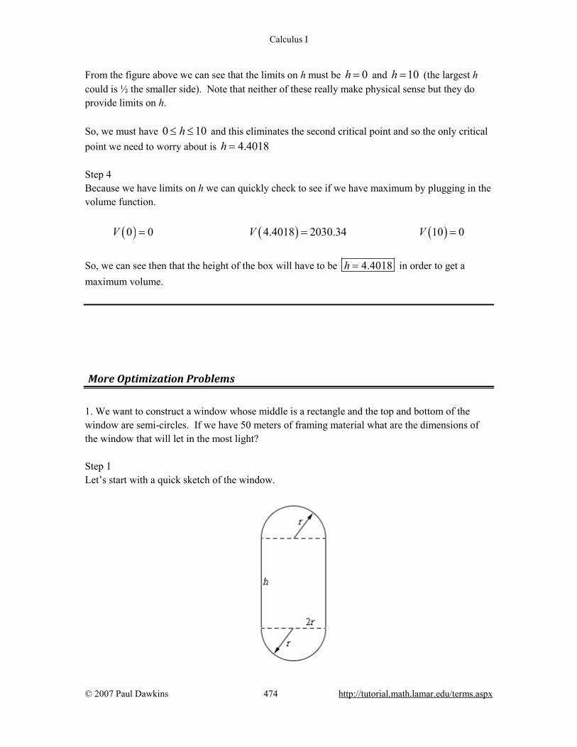
Calculus I
© 2007 Paul Dawkins 474 http://tutorial.math.lamar.edu/terms.aspx
From the figure above we can see that the limits on h must be 0h = and 10h = (the largest h could is ½ the smaller side). Note that neither of these really make physical sense but they do provide limits on h. So, we must have 0 10h≤ ≤ and this eliminates the second critical point and so the only critical point we need to worry about is 4.4018h = Step 4 Because we have limits on h we can quickly check to see if we have maximum by plugging in the volume function. ( ) ( ) ( )0 0 4.4018 2030.34 10 0V V V= = =
So, we can see then that the height of the box will have to be 4.4018h = in order to get a maximum volume.
More Optimization Problems 1. We want to construct a window whose middle is a rectangle and the top and bottom of the window are semi-circles. If we have 50 meters of framing material what are the dimensions of the window that will let in the most light? Step 1 Let’s start with a quick sketch of the window.
Calculus I
© 2007 Paul Dawkins 475 http://tutorial.math.lamar.edu/terms.aspx
Step 2 Next we need to set up the constraint and equation that we are being asked to optimize. We are told that we have 50 meters of framing material (i.e. the perimeter of the window) and so that will be the constraint for this problem. ( )50 2 2 2 2h r h rπ π= + = + We are being asked to maximize the amount of light being let in and that is simply the enclosed area or, ( ) ( )2 21
22 2 2A h r r hr rπ π= + = + With both of these equations we were a little careful with the last term. In each case we needed either the perimeter or area of each semicircle and there were two of them. The end result of course is the equation of the perimeter/area of a whole circle, but we really should be careful setting these equations up and note just where everything is coming from. Step 3 Now, let’s solve the constraint for h. 25h rπ= − Plugging this into the area function gives, ( ) ( ) 2 22 25 50A r r r r r rπ π π= − + = − Step 4 Finding the critical point(s) for this shouldn’t be too difficult at this point. Here is the derivative. ( ) 50 2A r rπ′ = − From this it looks like we get a single critical points are : 25 7.9577r π= = . Step 5 The second derivative of the volume function is, ( ) 2A r π′′ = − From this we can see that the second derivative is always negative. Therefore ( )A r will always
be concave down and so the single critical point we got in Step 4 must be a relative maximum and hence must be the value that allows in the maximum amount of light. Step 6

Calculus I
© 2007 Paul Dawkins 476 http://tutorial.math.lamar.edu/terms.aspx
Now, let’s finish the problem by getting the radius of the semicircles. ( )2525 0h ππ= − = Okay, what this means is that in fact the most light will come from not even having a rectangle between the semicircles and just having a circular window of radius 25r π= . 2. Determine the area of the largest rectangle that can be inscribed in a circle of radius 1. Step 1 Let’s start with a quick sketch of the circle and rectangle. Also, in order to make the work a little easier we went ahead and assumed that the circle was centered at the origin of the standard xy-coordinate system. We’ve also defined a point ( ),x y in the first quadrant. This is the point that we will be
attempting to find when we get into the problems. If we know the coordinates of this point then the rectangle defined by the point, as shown in the figure, will be the one with the largest area.
Step 2 Next we need to set up the constraint and equation that we are being asked to optimize. Given our graph above we can easily determine the equation of the circle. This will also be the constraint of the problem because the corners of the rectangle must be on the circle. 2 2 1x y+ =

Calculus I
© 2007 Paul Dawkins 477 http://tutorial.math.lamar.edu/terms.aspx
Also note that from the figure or equation we can clearly see that 1 1x− ≤ ≤ and 1 1y− ≤ ≤ . One or both of these limits will be useful later on in the problem. We are being asked to maximize the amount of the rectangle and using the definitions we see in the figure above the area is, ( )( )2 2 4A x y xy= = Step 3 We can solve the constraint for x or y. Either will lead to essentially the same work so we’ll solve for x. 21x y= ± − Because we’ve defined the point on the circle to be in the 1st quadrant we will use the “+” portion of this. Plugging this into the area function gives,
( ) 24 1A y y y= − Step 4 Finding the critical point(s) for this shouldn’t be too difficult at this point. Here is the derivative.
( )2 2
2
2 2
4 4 84 11 1
y yA y yy y
−′ = − − =− −
From this it looks like, from the numerator, we get the critical points,
1 12 2
0.7071y = ± = ± = ±
From the denominator we get the critical points : 1y = ± . Before proceeding to the next step let’s notice that because our point is in the first quadrant we know that y must be positive. This fact along with the limits on y we discussed in Step 2 tells us that we must have : 0 1y≤ ≤ . This in turn tells us that the only two critical points that we need to worry about are,
12
0.7071 1y y= = =
Step 5 Because we’ve got a range for possible critical points all we need to do to determine the maximum area is plug the end points and critical points into the area.

Calculus I
© 2007 Paul Dawkins 478 http://tutorial.math.lamar.edu/terms.aspx
( ) ( ) ( )12
0 2 1 0A A A= = Step 6 So, the area of the largest rectangle that can be inscribed in the circle is : 2. 3. Find the point(s) on 23 2x y= − that are closest to ( )4,0− .
Step 1 Let’s start with a quick sketch of this situation. Below is a sketch of the graph of the function as well as the point ( )4,0− . As we can see we can expect to get two points as answers with the
only difference being the sign on the y-coordinate.
Step 2 Next we need to set up the constraint and equation that we are being asked to optimize. In this case the constraint is simply the equation we are given. The point must lie on the graph and so must also satisfy the equation. 23 2x y= − We are being asked to minimize the distance between a point (or points) on the graph and the point ( )4,0− . We can do this by looking at the distance between ( )4,0− and ( ),x y . The distance between these two points is,
( )2 24d x y= + +

Calculus I
© 2007 Paul Dawkins 479 http://tutorial.math.lamar.edu/terms.aspx
As we discussed in the notes for this section the point that minimizes the square of the distance will also minimize the distance itself and so to avoid dealing with the root we will minimize the square of the distance or,
( )22 24d x y= + + Step 3 Now we have two choices on how to proceed from this point. The first option is to plug the equation we are given into the x in the distance squared and get a 4th degree polynomial for y that we’ll need to work with. The second is to solve the equation for
2y and plug that into the distance squared and get a 2nd degree polynomial for x that we’ll need to work with. The second option gives a “nicer” polynomial to work with so we’ll do that. ( )2 31 1
2 2 23y x x= − = − Plugging this into the distance squared gives,
( ) ( )22 23 15 3512 2 2 24f x d x x x x= = + + − = + +
Step 4 Finding the critical point(s) for this shouldn’t be too difficult at this point. Here is the derivative. ( ) 15
22f x x′ = + From this it looks like we get a single critical point : 15
4 3.75x = − = − . Step 5 The second derivative of the distance squared function is, ( ) 2f x′′ = From this we can see that the second derivative is always positive. Therefore the distance squared will always be concave up and so the single critical point we got in Step 4 must be a relative minimum and hence must be the value of x that gives the points that are closest to
( )4,0− .
Step 6 Finally we just need to determine the values y that give the actual points.
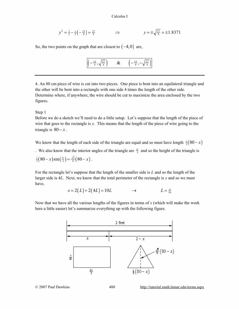
Calculus I
© 2007 Paul Dawkins 480 http://tutorial.math.lamar.edu/terms.aspx
( )2 3 15 27 2712 2 4 8 8 1.8371y y= − − = ⇒ = ± = ±
So, the two points on the graph that are closest to ( )4,0− are,
( ) ( )15 27 15 274 4 4 4, & ,− − −
4. An 80 cm piece of wire is cut into two pieces. One piece is bent into an equilateral triangle and the other will be bent into a rectangle with one side 4 times the length of the other side. Determine where, if anywhere, the wire should be cut to maximize the area enclosed by the two figures. Step 1 Before we do a sketch we’ll need to do a little setup. Let’s suppose that the length of the piece of wire that goes to the rectangle is x. This means that the length of the piece of wire going to the triangle is 80 x− . We know that the length of each side of the triangle are equal and so must have length ( )1
3 80 x−
. We also know that the interior angles of the triangle are 3π and so the height of the triangle is
( ) ( ) ( )313 3 680 sin 80x xπ− = − .
For the rectangle let’s suppose that the length of the smaller side is L and so the length of the larger side is 4L. Next, we know that the total perimeter of the rectangle is x and so we must have, ( ) ( ) 102 2 4 10 xx L L L L= + = → = Now that we have all the various lengths of the figures in terms of x (which will make the work here a little easier) let’s summarize everything up with the following figure.

Calculus I
© 2007 Paul Dawkins 481 http://tutorial.math.lamar.edu/terms.aspx
Step 2 Next we need to set up the constraint and equation that we are being asked to optimize. This is one of those cases where we really don’t have a constraint equation to work with. The constraint is the length of the wire (80 cm), but we took that into account when we set up our figure above so there isn’t anything to do with that in this case. We are being asked to maximize the enclosed area of the two figures and so here is the total area of the enclosed figures.
( ) ( ) ( ) ( ) ( ) ( )2 23 32 1 110 5 2 3 6 25 3680 80 80x x xA x x x x = + − − = + −
Step 3 Finding the critical point(s) for this shouldn’t be too difficult at this point (although the Algebra will be a little messy). Here is the derivative.
( ) ( )3225 18 80xA x x′ = − −
From this it looks like we get a single critical point,
40 3
932
25 18
43.6828x = =+
Step 4 The second derivative of the area function is,
( ) 3225 18A x′′ = +
From this we can see that the second derivative is always positive. Therefore ( )A x will always
be concave up and so the single critical point we got in Step 4 must be a relative minimum and hence must be the value of x (i.e. the cut point) that will give the minimum enclosed area. This is a problem however as we were asked for the maximum enclosed area. This is the reason for this step being in every problem that we’ve worked over the last couple of sections. Far too often students get to this point, get a single answer and then just assume that it must be the correct answer and don’t bother doing any kind of checking to verify if it is the correct answer. After all there was a single value so there is no choice for it to be correct. Right? Well, no. As we’ll seen here it in fact is not the correct answer. Step 5

Calculus I
© 2007 Paul Dawkins 482 http://tutorial.math.lamar.edu/terms.aspx
So, what to do? We’ll recall for the problem statement that we were asked to, “Determine where, if anywhere, the wire should be cut to maximize the area enclosed by the two figures.” The “if anywhere” portion seems to suggest that we may not want to cut it at all. Maybe all of the wire should go to the rectangle (corresponding to 80x = above) or maybe all of the wire should to the triangle (corresponding to 0x = above). So, all we need to do is plug 80x = and 0x = into the area function and determine which will give the largest area.
( )
( )( )
0 307.92 All wire goes to triangle.
43.6828 139.785 Wire goes to both triangle and rectangle.
80 256 All wire goes to rectangle.
A
A
A
=
=
=
Note that we included the critical point above just to make it really clear that it will not in fact give the maximum area. We didn’t really need to include it here as we already knew it wouldn’t work for us. From the function evaluations above it looks like we’ll need to take all of the wire and bend it into an equilateral triangle in order to get the maximum area. 5. A line through the point ( )2,5 forms a right triangle with the x-axis and y-axis in the 1st
quadrant. Determine the equation of the line that will minimize the area of this triangle. Step 1 This problem may seem a little tricky at first. Here is a sketch of a line that goes through the point ( )2,5 , has an x-intercept of ( ),0a and a y-intercept of ( )0,b .
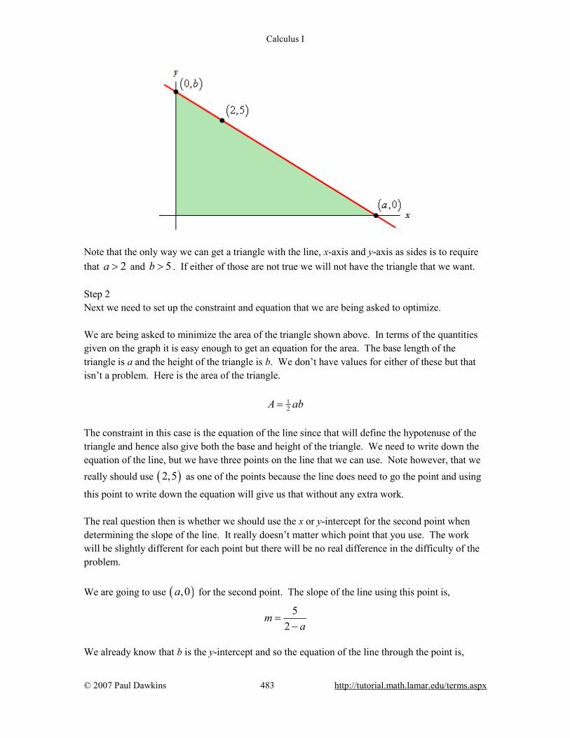
Calculus I
© 2007 Paul Dawkins 483 http://tutorial.math.lamar.edu/terms.aspx
Note that the only way we can get a triangle with the line, x-axis and y-axis as sides is to require that 2a > and 5b > . If either of those are not true we will not have the triangle that we want. Step 2 Next we need to set up the constraint and equation that we are being asked to optimize. We are being asked to minimize the area of the triangle shown above. In terms of the quantities given on the graph it is easy enough to get an equation for the area. The base length of the triangle is a and the height of the triangle is b. We don’t have values for either of these but that isn’t a problem. Here is the area of the triangle. 1
2A ab= The constraint in this case is the equation of the line since that will define the hypotenuse of the triangle and hence also give both the base and height of the triangle. We need to write down the equation of the line, but we have three points on the line that we can use. Note however, that we really should use ( )2,5 as one of the points because the line does need to go the point and using
this point to write down the equation will give us that without any extra work. The real question then is whether we should use the x or y-intercept for the second point when determining the slope of the line. It really doesn’t matter which point that you use. The work will be slightly different for each point but there will be no real difference in the difficulty of the problem. We are going to use ( ),0a for the second point. The slope of the line using this point is,
52
ma
=−
We already know that b is the y-intercept and so the equation of the line through the point is,

Calculus I
© 2007 Paul Dawkins 484 http://tutorial.math.lamar.edu/terms.aspx
52
y x ba
= +−
Note that we definitely seem to have a problem here. Normally at this point we’ve got two equation and two unknowns. In this case we appear to have four unknowns : a, b, x and y. This isn’t a problem as well see in the next step. Step 3 We now need to solve the constraint for one of the unknowns in the area function, i.e either a or b. However, as we noted above we also have an x and y in the equation that will cause problems if they stay in the equation. The point of this step is to get the area function down to a single variable. If we leave the x and y in the equation of the line we will end up with an area function with not one variable but three and that won’t work for us. What we really need is an equation involving only a and b that we can solve for one or the other and plug into the area function. Luckily this is easy to get. All we need to do is plug the x-intercept into the equation of the line to get,
502
a ba
= +−
Do you see why we couldn’t have used the y-intercept here? If not, plug it in and you’ll very quickly see why it won’t work. At this point we can easily solve the equation for b to get,
5 52 2
a aba a
= − =− −
To eliminate one of the minus signs we took the minus sign in front of the quotient and applied it to the denominator and simplified. This doesn’t need to be done, but it does eliminate one of them. Note that if we had used the y-intercept to determine the slope we would have found it to be easier at this step to solve for a instead. That is the only real difference in which point you use to find the slope. Okay, let’s put all this together. We know the value of b in terms of a so plug that into the area function to get,
( ) ( )21 5 5
2 2 2 2a aA a a
a a = = − −
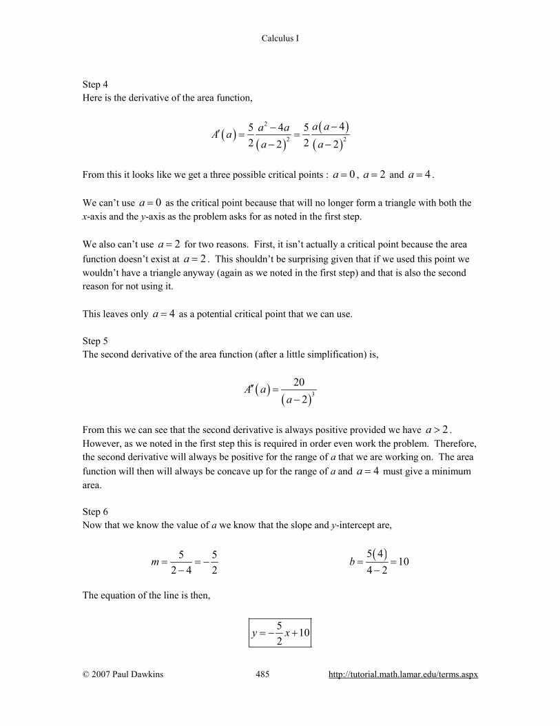
Calculus I
© 2007 Paul Dawkins 485 http://tutorial.math.lamar.edu/terms.aspx
Step 4 Here is the derivative of the area function,
( )( )
( )( )
2
2 2
45 4 52 22 2
a aa aA aa a
−−′ = =− −
From this it looks like we get a three possible critical points : 0a = , 2a = and 4a = . We can’t use 0a = as the critical point because that will no longer form a triangle with both the x-axis and the y-axis as the problem asks for as noted in the first step. We also can’t use 2a = for two reasons. First, it isn’t actually a critical point because the area function doesn’t exist at 2a = . This shouldn’t be surprising given that if we used this point we wouldn’t have a triangle anyway (again as we noted in the first step) and that is also the second reason for not using it. This leaves only 4a = as a potential critical point that we can use. Step 5 The second derivative of the area function (after a little simplification) is,
( )( )3
202
A aa
′′ =−
From this we can see that the second derivative is always positive provided we have 2a > . However, as we noted in the first step this is required in order even work the problem. Therefore, the second derivative will always be positive for the range of a that we are working on. The area function will then will always be concave up for the range of a and 4a = must give a minimum area. Step 6 Now that we know the value of a we know that the slope and y-intercept are,
( )5 45 5 102 4 2 4 2
m b= = − = =− −
The equation of the line is then,
5 102
y x= − +

Calculus I
© 2007 Paul Dawkins 486 http://tutorial.math.lamar.edu/terms.aspx
6. A piece of pipe is being carried down a hallway that is 18 feet wide. At the end of the hallway there is a right-angled turn and the hallway narrows down to 12 feet wide. What is the longest pipe (always keeping it horizontal) that can be carried around the turn in the hallway? Step 1 Let’s start with a quick sketch of the pipe and hallways with all the important quantities given.
Step 2 Next we need to set up the constraint and equation that we are being asked to optimize. As we discussed in the similar problem in the notes for this section we actually need to minimize the total length of the pipe. The equation we need to minimize is then, 1 2L L L= + Also as we discussed in the notes problem with actually have two constraints : the widths of the two hallways. We can easily solve for these in terms of the angle θ . 1 212sec 18cscL Lθ θ= = As discussed in the notes problem we also know that we must have 20 πθ< < . Step 3 All we need to do here is plug our two constraints in the length function to get a function in terms of θ that we can minimize. ( ) 12sec 18cscL θ θ θ= + Step 4
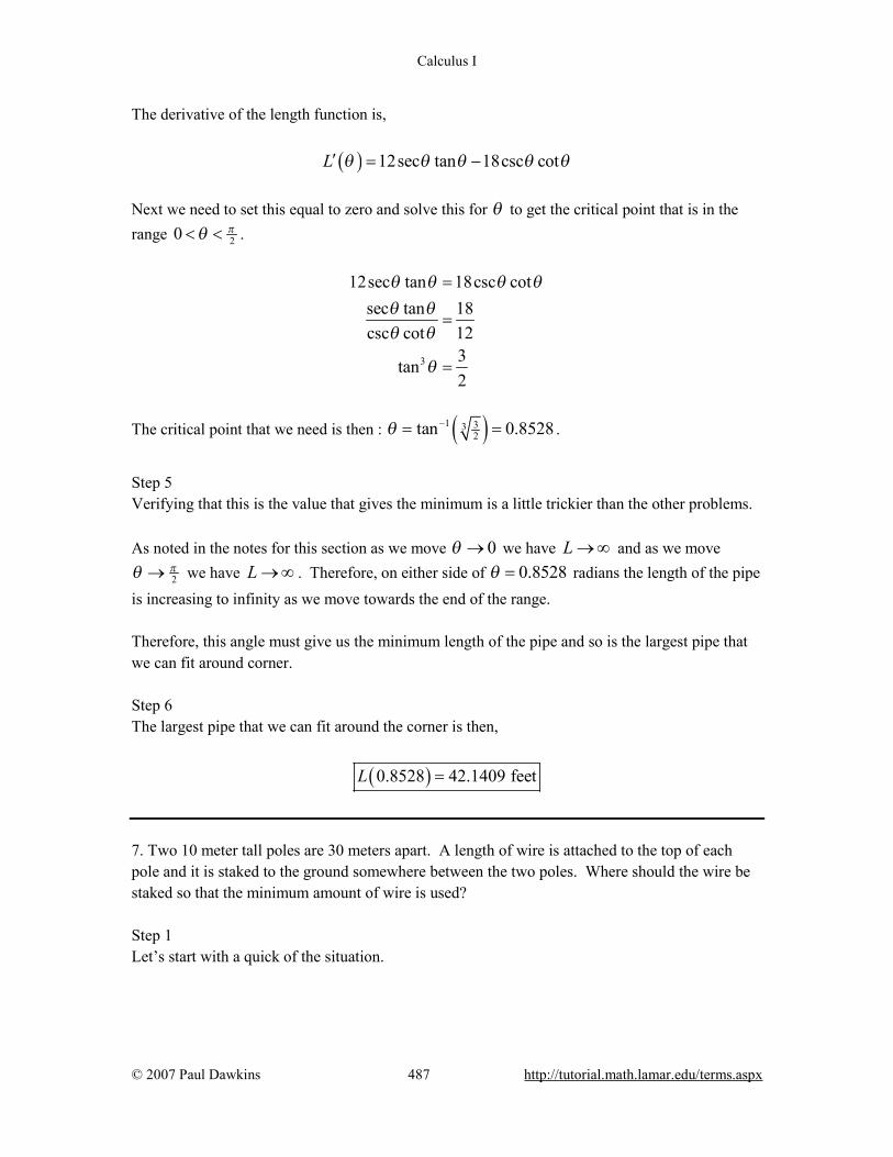
Calculus I
© 2007 Paul Dawkins 487 http://tutorial.math.lamar.edu/terms.aspx
The derivative of the length function is, ( ) 12sec tan 18csc cotL θ θ θ θ θ′ = − Next we need to set this equal to zero and solve this for θ to get the critical point that is in the range 20 πθ< < .
3
12sec tan 18csc cotsec tan 18csc cot 12
3tan2
θ θ θ θθ θθ θ
θ
=
=
=
The critical point that we need is then : ( )1 332tan 0.8528θ −= = .
Step 5 Verifying that this is the value that gives the minimum is a little trickier than the other problems. As noted in the notes for this section as we move 0θ → we have L → ∞ and as we move
2πθ → we have L → ∞ . Therefore, on either side of 0.8528θ = radians the length of the pipe
is increasing to infinity as we move towards the end of the range. Therefore, this angle must give us the minimum length of the pipe and so is the largest pipe that we can fit around corner. Step 6 The largest pipe that we can fit around the corner is then,
( )0.8528 42.1409 feetL = 7. Two 10 meter tall poles are 30 meters apart. A length of wire is attached to the top of each pole and it is staked to the ground somewhere between the two poles. Where should the wire be staked so that the minimum amount of wire is used? Step 1 Let’s start with a quick of the situation.
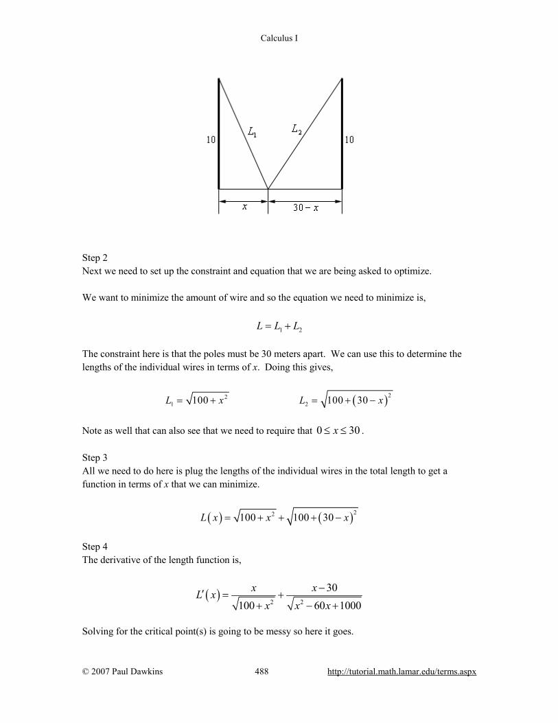
Calculus I
© 2007 Paul Dawkins 488 http://tutorial.math.lamar.edu/terms.aspx
Step 2 Next we need to set up the constraint and equation that we are being asked to optimize. We want to minimize the amount of wire and so the equation we need to minimize is, 1 2L L L= + The constraint here is that the poles must be 30 meters apart. We can use this to determine the lengths of the individual wires in terms of x. Doing this gives,
( )221 2100 100 30L x L x= + = + −
Note as well that can also see that we need to require that 0 30x≤ ≤ . Step 3 All we need to do here is plug the lengths of the individual wires in the total length to get a function in terms of x that we can minimize.
( ) ( )22100 100 30L x x x= + + + − Step 4 The derivative of the length function is,
( )2 2
30100 60 1000
x xL xx x x
−′ = ++ − +
Solving for the critical point(s) is going to be messy so here it goes.

Calculus I
© 2007 Paul Dawkins 489 http://tutorial.math.lamar.edu/terms.aspx
( )( ) ( ) ( )
2 2
2 2
2 2
22 2 2
4 3 2 4 3 2
30 0100 60 1000
30100 60 1000
60 1000 30 100
60 1000 30 100
60 1000 60 1000 6000 900000 6000 90000
15
x xx x x
x xx x x
x x x x x
x x x x x
x x x x x x xx
x
−+ =
+ − +−
= −+ − +
− + = − − +
− + = − +
− + = − + − += − +=
A quick check by plugging this back into the derivative shows that we do indeed get ( )15 0L′ =
and so this is a critical point and it is in the acceptable range of x. Recall that because we squared both sides of the equation above it is possible to end up with answers that in fact are not solutions and so we have to go back and check in the original equation to make sure that they are solutions. Step 5 Since we have a range of x’s and the distance function is continuous in the range all we need to do is plug in the endpoints and the critical point to identify the minimum distance. ( ) ( ) ( )0 41.6228 15 36.0555 30 41.6228L L L= = = Step 6 The wire should be staked midway between the poles to minimize the amount of wire.
Indeterminate Forms and L’Hospital’s Rule
1. Use L’Hospital’s Rule to evaluate 3 2
22
7 10lim6x
x x xx x→
− ++ −
.
Step 1 The first step we should really do here is verify that L’Hospital’s Rule can in fact be used on this limit.
Calculus I
© 2007 Paul Dawkins 490 http://tutorial.math.lamar.edu/terms.aspx
This may seem like a silly step given that we are told to use L’Hospital’s Rule. However, in later sections we won’t be told to use it when/if it can be used. Therefore, we really need to get in the habit of checking that it can be used before applying it just to make sure that we can. If we apply L’Hospital’s Rule to a problem that it can’t be applied to then it’s is almost assured that we will get the wrong answer (it’s always possible you might get lucky and get the correct answer, but we will only be very lucky if it does). So a quick check shows us that,
3 2
2
7 10 0as 26 0
x x xxx x− +
→ →+ −
and so this is a form that allows the use of L’Hospital’s Rule. Step 2 So, at this point let’s just apply L’Hospital’s Rule.
3 2 2
22 2
7 10 3 14 10lim lim6 2 1x x
x x x x xx x x→ →
− + − +=
+ − +
Step 3 At this point all we need to do is try the limit and see if it can be done.
3 2 2
22 2
7 10 3 14 10 6lim lim6 2 1 5x x
x x x x xx x x→ →
− + − + −= =
+ − + So, the limit can be done and we done with the problem! The limit is then,
3 2
22
7 10 6lim6 5x
x x xx x→
− += −
+ −
2. Use L’Hospital’s Rule to evaluate ( )
24
sinlim
16w
ww
π→− −
.
Step 1 The first step we should really do here is verify that L’Hospital’s Rule can in fact be used on this limit. This may seem like a silly step given that we are told to use L’Hospital’s Rule. However, in later sections we won’t be told to use it when/if it can be used. Therefore, we really need to get in the habit of checking that it can be used before applying it just to make sure that we can. If we apply L’Hospital’s Rule to a problem that it can’t be applied to then it’s is almost assured that we will
Calculus I
© 2007 Paul Dawkins 491 http://tutorial.math.lamar.edu/terms.aspx
get the wrong answer (it’s always possible you might get lucky and get the correct answer, but we will only be very lucky if it does). So a quick check shows us that,
( )2
sin 0as 416 0w
ww
π→ − →
− and so this is a form that allows the use of L’Hospital’s Rule. Step 2 So, at this point let’s just apply L’Hospital’s Rule.
( ) ( )
24 4
sin coslim lim
16 2w w
w ww w
π π π→− →−
=−
Step 3 At this point all we need to do is try the limit and see if it can be done.
( ) ( ) ( )24 4
sin cos cos 4lim lim
16 2 8 8w w
w ww w
π π π π π π→− →−
−= = =
− − − So, the limit can be done and we done with the problem! The limit is then,
( )24
sinlim
16 8w
ww
π π→−
= −−
3. Use L’Hospital’s Rule to evaluate ( )
2
ln 3limt
tt→∞
.
Step 1 The first step we should really do here is verify that L’Hospital’s Rule can in fact be used on this limit. This may seem like a silly step given that we are told to use L’Hospital’s Rule. However, in later sections we won’t be told to use it when/if it can be used. Therefore, we really need to get in the habit of checking that it can be used before applying it just to make sure that we can. If we apply L’Hospital’s Rule to a problem that it can’t be applied to then it’s is almost assured that we will get the wrong answer (it’s always possible you might get lucky and get the correct answer, but we will only be very lucky if it does). So a quick check shows us that,

Calculus I
© 2007 Paul Dawkins 492 http://tutorial.math.lamar.edu/terms.aspx
( )2
ln 3as
tt
t∞
→ ∞ →∞
and so this is a form that allows the use of L’Hospital’s Rule. Step 2 So, at this point let’s just apply L’Hospital’s Rule.
( ) 1
2 2
ln 3 1lim lim lim2 2
tt t t
tt t t→∞ →∞ →∞
= =
Don’t forget to simplify after taking the derivatives. This can often be the difference between being able to do the problem or not. Step 3 At this point all we need to do is try the limit and see if it can be done.
( )2 2
ln 3 1lim lim 02t t
tt t→∞ →∞
= = So, the limit can be done and we done with the problem! The limit is then,
( )2
ln 3lim 0t
tt→∞
=
4. Use L’Hospital’s Rule to evaluate ( )
( )
2
220
sin 2 7 2lim
1z
z z zz z→
+ −
+.
Step 1 The first step we should really do here is verify that L’Hospital’s Rule can in fact be used on this limit. This may seem like a silly step given that we are told to use L’Hospital’s Rule. However, in later sections we won’t be told to use it when/if it can be used. Therefore, we really need to get in the habit of checking that it can be used before applying it just to make sure that we can. If we apply L’Hospital’s Rule to a problem that it can’t be applied to then it’s is almost assured that we will get the wrong answer (it’s always possible you might get lucky and get the correct answer, but we will only be very lucky if it does). So a quick check shows us that,

Calculus I
© 2007 Paul Dawkins 493 http://tutorial.math.lamar.edu/terms.aspx
( )( )
2
22
sin 2 7 2 0as 001
z z zz
z z+ −
→ →+
and so this is a form that allows the use of L’Hospital’s Rule. Step 2 Before actually using L’Hospital’s Rule it might be better if we multiply out the denominator to make the derivative (and later steps a little easier). Doing this gives,
( )
( )( )2 2
2 4 3 220 0
sin 2 7 2 sin 2 7 2lim lim
21z z
z z z z z zz z zz z→ →
+ − + −=
+ ++
Now let’s apply L’Hospitals’s Rule.
( )( )
( )2
2 3 220 0
sin 2 7 2 2cos 2 14 2lim lim
4 6 21z z
z z z z zz z zz z→ →
+ − + −=
+ ++
Step 3 At this point let’s try the limit and see if it can be done. However, in this case, we can see that,
( )3 2
2cos 2 14 2 0as 04 6 2 0
z zz
z z z+ −
→ →+ +
Step 4 So, using L’Hospital’s Rule doesn’t give us a limit that we can do. However, the new limit is one that can use L’Hospital’s Rule on so let’s do that.
( )( )
( )2
2 220 0
sin 2 7 2 4sin 2 14 14lim lim12 12 2 21z z
z z z zz zz z→ →
+ − − += =
+ ++
Okay, the second L’Hospital’s Rule gives us a limit we can do and so the answer is,
( )( )
2
220
sin 2 7 2lim 7
1z
z z zz z→
+ −=
+
5. Use L’Hospital’s Rule to evaluate 2
1limx x
x−→−∞ e
.
Calculus I
© 2007 Paul Dawkins 494 http://tutorial.math.lamar.edu/terms.aspx
Step 1 The first step we should really do here is verify that L’Hospital’s Rule can in fact be used on this limit. This may seem like a silly step given that we are told to use L’Hospital’s Rule. However, in later sections we won’t be told to use it when/if it can be used. Therefore, we really need to get in the habit of checking that it can be used before applying it just to make sure that we can. If we apply L’Hospital’s Rule to a problem that it can’t be applied to then it’s is almost assured that we will get the wrong answer (it’s always possible you might get lucky and get the correct answer, but we will only be very lucky if it does). So a quick check shows us that,
2
1as xxx −
∞→ − ∞ →
∞e and so this is a form that allows the use of L’Hospital’s Rule. Step 2 So, at this point let’s just apply L’Hospital’s Rule.
2
1 1
2lim limx xx x
x x− −→−∞ →−∞
=−e e
Step 3 At this point let’s try the limit and see if it can be done. However, in this case, we can see that,
1
2as xxx −
−∞→ − ∞ →
− −∞e Step 4 So, using L’Hospital’s Rule doesn’t give us a limit that we can do. However, the new limit is one that can use L’Hospital’s Rule on so let’s do that.
2
1 1 1
2 2lim lim lim 0x x xx x x
x x− − −→−∞ →−∞ →−∞
= = =−e e e
Okay, the second L’Hospital’s Rule gives us a limit we can do and so the answer is,
2
1lim 0x x
x−→−∞
=e
6. Use L’Hospital’s Rule to evaluate 2 4
lim2z
z
zz
z→∞
+−
ee
.
Calculus I
© 2007 Paul Dawkins 495 http://tutorial.math.lamar.edu/terms.aspx
Step 1 The first step we should really do here is verify that L’Hospital’s Rule can in fact be used on this limit. This may seem like a silly step given that we are told to use L’Hospital’s Rule. However, in later sections we won’t be told to use it when/if it can be used. Therefore, we really need to get in the habit of checking that it can be used before applying it just to make sure that we can. If we apply L’Hospital’s Rule to a problem that it can’t be applied to then it’s is almost assured that we will get the wrong answer (it’s always possible you might get lucky and get the correct answer, but we will only be very lucky if it does). So a quick check shows us that,
2 4
as2
z
zzz
z+ ∞
→ ∞ →− −∞
ee
and so this is a form that allows the use of L’Hospital’s Rule. Step 2 So, at this point let’s just apply L’Hospital’s Rule.
2 4 42 4lim lim
2 2z z
z z
z zz z
z→∞ →∞
+ +=
− −e ee e
Step 3 At this point let’s try the limit and see if it can be done. However, in this case, we can see that,
42 4as
2
z
zzz + ∞
→ ∞ →− −∞
ee
Step 4 So, using L’Hospital’s Rule doesn’t give us a limit that we can do. However, the new limit is one that can use L’Hospital’s Rule on so let’s do that.
2 4 4 42 4 2 16lim lim lim
2 2z z z
z z z
z z zz z
z→∞ →∞ →∞
+ + += =
− − −e e ee e e
Step 5 Now, at this point we need to be careful. It looks like we are still in a case of an infinity divided by an infinity and that looks to continue forever if we keep applying L’Hospital’s Rule. However, do not forget to do some basic simplifications where you can. If we simplify we get the following.

Calculus I
© 2007 Paul Dawkins 496 http://tutorial.math.lamar.edu/terms.aspx
( ) ( ) ( )2 4
4 3lim lim 2 16 lim 2 162z z z
zz z z z
zz
z→∞ →∞ →∞
− −+= + − = − −
−e e e e ee
and this is something that we can take the limit of. So the answer is,
( )2 4
3lim lim 2 162z z
zz z
zz
z→∞ →∞
−+= − − = −∞
−e e ee
Again, it cannot be stressed enough that you’ve got to do simplification where you can. For some of these problems that can mean the difference between being able to do the problem or not.
7. Use L’Hospital’s Rule to evaluate 3lim ln 1
tt
t→∞
+ .
Step 1 The first thing to notice here is that is not in a form that allows L’Hospital’s Rule. L’Hospital’s Rule only works on a certain class of rational functions and this is clearly not a rational function. Note however that it is in the following indeterminate form,
( ) ( )3as ln 1 0t tt
→ ∞ + → ∞
and as we discussed in the notes for this section we can always turn this kind of indeterminate form into a rational expression that will allow L’Hospital’s Rule to be applied. Step 2 The real question is do we move the first term or the second term to the denominator. From the looks of things it appears that it would be best to move the first term to the denominator.
3ln 13lim ln 1 lim 1t t
ttt t
→∞ →∞
+ + =
Notice as well that,
Calculus I
© 2007 Paul Dawkins 497 http://tutorial.math.lamar.edu/terms.aspx
3ln 10as 1 0
ttt
+ → ∞ →
and we can use L’Hospital’s Rule on this. Step 3 Applying L’Hospital’s Rule gives,
2
2
33ln 1 313lim ln 1 lim lim1 1t t t
tt tt
t t t→∞ →∞ →∞
− + + + = = −
Can you see why we chose to move the t to the denominator? Moving the logarithm would have left us with a very messy derivative to take! It might have ended up working okay for us, but the work would be greatly increased. Step 4 Do not forget to simplify after we’ve taken the derivative. This problem becomes very simple if we do that.
3ln 13 3lim ln 1 lim lim 31 31t t t
ttt t t
→∞ →∞ →∞
+ + = = = +
8. Use L’Hospital’s Rule to evaluate ( )2 2
0lim ln 4w
w w+→
.
Step 1 The first thing to notice here is that is not in a form that allows L’Hospital’s Rule. L’Hospital’s Rule only works on a certain class of rational functions and this is clearly not a rational function. Note however that it is in the following indeterminate form, ( ) ( ) ( )2 2as 0 ln 4 0w w w+→ → −∞ and as we discussed in the notes for this section we can always turn this kind of indeterminate form into a rational expression that will allow L’Hospital’s Rule to be applied. Step 2

Calculus I
© 2007 Paul Dawkins 498 http://tutorial.math.lamar.edu/terms.aspx
The real question is do we move the first term or the second term to the denominator. From the looks of things it appears that it would be best to move the first term to the denominator.
( ) ( )22 2
0 02
ln 4lim ln 4 lim 1w w
ww w
w+ +→ →
=
Notice as well that,
( )2
2
ln 4as 0 1
ww
w
+ −∞→ →
∞
and we can use L’Hospital’s Rule on this. Step 3 Applying L’Hospital’s Rule gives,
( ) ( )22 2
0 0 02 3
2ln 4lim ln 4 lim lim1 2w w w
w ww ww w
+ + +→ → → = = −
Can you see why we chose to move the first term to the denominator? Moving the logarithm would have left us with a very messy derivative to take! It might have ended up working okay for us, but the work would be greatly increased. Step 4 Do not forget to simplify after we’ve taken the derivative. This problem becomes very simple if we do that. In fact, it is the only way to actually get an answer for this problem. If we do not simplify will get stuck in a never ending chain of infinity divided by infinity forms no matter how many times we apply L’Hospital’s Rule.
( ) ( ) ( )2
2 2 2
0 0 02
ln 4lim ln 4 lim lim 01w w w
ww w w
w+ + +→ → →
= = − =
9. Use L’Hospital’s Rule to evaluate ( ) ( )21lim 1 tanx
x xπ+→
− .
Step 1 The first thing to notice here is that is not in a form that allows L’Hospital’s Rule. L’Hospital’s Rule only works on a certain class of rational functions and this is clearly not a rational function. Note however that it is in the following indeterminate form,

Calculus I
© 2007 Paul Dawkins 499 http://tutorial.math.lamar.edu/terms.aspx
( ) ( ) ( ) ( )2as 1 1 tan 0x x xπ+→ − → ∞ and as we discussed in the notes for this section we can always turn this kind of indeterminate form into a rational expression that will allow L’Hospital’s Rule to be applied. Step 2 The real question is do we move the first term or the second term to the denominator. At first glance it might appear that neither term will be particularly useful in the denominator. In particular, if we move the tangent to the denominator we would end up needing to differentiate a
term in the form 1tan . That doesn’t look to be all that fun to differentiate and we’re liable to
end up with a mess when we are done. However, that is exactly the term we are going to move to the denominator for reasons that will quickly become apparent.
( ) ( )( ) ( )21 1 1
22
1 1lim 1 tan lim lim1 cottan
x x x
x xx xx
x
ππ
π+ + +→ → →
− − − = =
Step 3 With a little simplification after moving the tangent to the denominator we ended up with something that doesn’t look all that bad. We’ll also see that the remainder of this problem is going to be quite simple. Before we proceed however we should notice as well that,
( )2
1 0as 1cot 0
xxxπ
+ −→ →
and we can use L’Hospital’s Rule on this. Step 4 Applying L’Hospital’s Rule gives,
( ) ( ) ( ) ( )2 21 1 12 2 2
1 1 2lim 1 tan lim limcot cscx x x
xx xx x
ππ π π π+ + +→ → →
− − = = = − −
10. Use L’Hospital’s Rule to evaluate ( ) 21
0lim cos 2y
yy+→
.
Step 1
Calculus I
© 2007 Paul Dawkins 500 http://tutorial.math.lamar.edu/terms.aspx
The first thing to notice here is that is not in a form that allows L’Hospital’s Rule. L’Hospital’s Rule only works on certain classes of rational functions and this is clearly not a rational function. Note however that it is in the following indeterminate form,
( ) 21
as 0 cos 2 1yy y+ ∞→ → and as we discussed in the notes for this section we can do some manipulation on this to turn it into a problem that can be done with L’Hospital’s Rule. Step 2 First, let’s define,
( ) 21
cos 2 yz y= and take the log of both sides. We’ll also do a little simplification.
( )( ) ( ) ( )22
11
2
ln cos 2ln ln cos 2 ln cos 2y
y
yz y y
y = = =
Step 3 We can now take the limit as 0y +→ of this.
[ ] ( )20 0
ln cos 2lim ln limy y
yz
y+ +→ →
=
Before we proceed let’s notice that we have the following,
( ) ( )2
ln cos 2 ln 1 0as 00 0
yy
y+ → → =
and we have a limit that we can use L’Hospital’s Rule on. Step 4 Applying L’Hospital’s Rule gives,
[ ] ( )( )
( ) ( )20 0 0 0
2sin 2ln cos 2 cos 2 tan 2
lim ln lim lim lim2y y y y
yy y y
zy y y+ + + +→ → → →
− − = = =
Step 5 We now have a limit that behaves like,

Calculus I
© 2007 Paul Dawkins 501 http://tutorial.math.lamar.edu/terms.aspx
( )tan 2 0as 00
yy
y+ −
→ →
and so we can use L’Hospital’s Rule on this as well. Doing this gives,
[ ] ( ) ( )2
0 0 0
tan 2 2sec 2lim ln lim lim 2
1y y y
y yz
y+ + +→ → →
− −= = = −
Step 6 Now all we need to do is recall that, ln zz = e This in turn means that we can do the original limit as follows,
( )[ ]
2 0ln1 2
0 0 0
limlnlim cos 2 lim lim y
zz
y y yyy z +→
+ + +
−
→ → →= = = = e e e
11. Use L’Hospital’s Rule to evaluate 1
limx
x xx→∞
+ e .
Step 1 The first thing to notice here is that is not in a form that allows L’Hospital’s Rule. L’Hospital’s Rule only works on certain classes of rational functions and this is clearly not a rational function. Note however that it is in the following indeterminate form,
1
0as x xx x → ∞ + → ∞ e and as we discussed in the notes for this section we can do some manipulation on this to turn it into a problem that can be done with L’Hospital’s Rule. Step 2 First, let’s define,
1x xz x = + e
and take the log of both sides. We’ll also do a little simplification.

Calculus I
© 2007 Paul Dawkins 502 http://tutorial.math.lamar.edu/terms.aspx
1
1ln
ln ln lnx
x xxx
xz x x
x
+ = + = + =
ee e
Step 3 We can now take the limit as x → ∞ of this.
[ ]ln
lim ln limx x
x xz
x→∞ →∞
+ =
e
Before we proceed let’s notice that we have the following,
ln
asx x
xx
+ ∞ → ∞ →=∞
e
and we have a limit that we can use L’Hospital’s Rule on. Step 4 Applying L’Hospital’s Rule gives,
[ ]1ln 1lim ln lim lim lim1x x x x
xx xx
x
x xzx x→∞ →∞ →∞ →∞
+ + + + = = =+
ee eee
Step 5 We now have a limit that behaves like,
1asx
xxx
+ ∞→ ∞ →
+ ∞ee
and so we can use L’Hospital’s Rule on this as well. Doing this gives,
[ ] ( )1lim ln lim lim lim lim 1 11x x x x x
x x x
x x xzx→∞ →∞ →∞ →∞ →∞
+= = = = =
+ +e e ee e e
Notice that we did have to use L’Hospital’s Rule twice here and we also made sure to do some simplification so we could actually take the limit. Step 6 Now all we need to do is recall that, ln zz = e

Calculus I
© 2007 Paul Dawkins 503 http://tutorial.math.lamar.edu/terms.aspx
This in turn means that we can do the original limit as follows,
[ ]1 lnlimlnlim lim lim x
zz
x x x
x xx z →∞
→∞ →∞ →∞ + = = = = e e e e
Linear Approximations 1. Find a linear approximation to ( ) 2 103 xf x x −= e at 5x = .
Step 1 We’ll need the derivative first as well as a couple of function evaluations. ( ) ( ) ( )2 10 2 103 6 5 15 5 33x xf x x f f− −′ ′= + = =e e Step 2 There really isn’t much to do at this point other than write down the linear approximation.
( ) ( )15 33 5 33 150L x x x= + − = − While it wasn’t asked for, here is a quick sketch of the function and the linear approximation.

Calculus I
© 2007 Paul Dawkins 504 http://tutorial.math.lamar.edu/terms.aspx
2. Find a linear approximation to ( ) 4 36 3 7h t t t t= − + − at 3t = − .
Step 1 We’ll need the derivative first as well as a couple of function evaluations. ( ) ( ) ( )3 24 18 3 3 227 3 267h t t t h h′ ′= − + − = − = − Step 2 There really isn’t much to do at this point other than write down the linear approximation.
( ) ( )227 267 3 267 574L t t t= − + = − − While it wasn’t asked for, here is a quick sketch of the function and the linear approximation.
3. Find the linear approximation to ( ) 4g z z= at 2z = . Use the linear approximation to
approximate the value of 4 3 and 4 10 . Compare the approximated values to the exact values. Step 1 We’ll need the derivative first as well as a couple of function evaluations.
( ) ( ) ( ) ( )3 314 4 41 1
4 42 2 2 2g z z g g− −′ ′= = =
Step 2 Here is the linear approximation.
Calculus I
© 2007 Paul Dawkins 505 http://tutorial.math.lamar.edu/terms.aspx
( ) ( )( )31
4 4142 2 2L z z−= + −
Step 3 Finally here are the approximations of the values along with the exact values.
( ) ( )( ) ( )3 1.33786 3 1.31607 % Error : 1.65523
10 2.37841 10 1.77828 % Error : 33.7481
L g
L g
= =
= =
So, as we might have expected the farther from 2z = we got the worse the approximation is. Recall that the approximation will generally be more accurate the closer to the point of the linear approximation. 4. Find the linear approximation to ( ) ( )cos 2f t t= at 1
2t = . Use the linear approximation to
approximate the value of ( )cos 1 and ( )cos 9 . Compare the approximated values to the exact
values. Step 1 We’ll need the derivative first as well as a couple of function evaluations. ( ) ( ) ( ) ( ) ( ) ( )1 1
2 22sin 2 cos 1 2sin 1f t t f f′ ′= − = = − Step 2 Here is the linear approximation.
( ) ( ) ( ) ( ) ( )1 12 2cos 1 2sin 1 0.5403 1.6829L t t t= − − = − −
Make sure your calculator is set in radians! Remember that we use radians by default in this class. Step 3 Finally here are the approximations of the values along with the exact values.
( ) ( )( ) ( )1 0.301169 1 0.416147 % Error : 27.6292
9 13.7647 9 0.660317 % Error : 2184.56
L f
L f
= − = −
= − =
Calculus I
© 2007 Paul Dawkins 506 http://tutorial.math.lamar.edu/terms.aspx
So, as we might have expected the farther from 12t = we got the worse the approximation is.
Recall that the approximation will generally be more accurate the closer to the point of the linear approximation. 5. Without using any kind of computational aid use a linear approximation to estimate the value of 0.1e . Hint : This is really nothing more than Problem 3 and 4 from this section. The only difference is that you need to determine the function and the point for the linear approximation. The function should be pretty obvious given the value we are asked to estimate. There should also be a pretty obvious point to use given that we aren’t supposed to use calculators/computers. Step 1 This is really the same problem as Problems 3 & 4 from this section. The difference is that we need to determine the function and point for the linear approximation. Given the value we are being asked to estimate it should be fairly clear that the function should be,
( ) xf x = e
The point for the linear approximation should also be somewhat clear. With the function in hand it’s now clear that we are being asked to use a linear approximation to estimate ( )0.1f . So,
we’ll need a point that is close to 0.1x = and one that we can evaluate in the function without a calculator. It therefore seems fairly clear that 0x = would be a really nice point use for the linear approximation. Step 2 At this point finding the linear approximation shouldn’t be too bad so here is the work for that. ( ) ( ) ( )0 1 0 1xf x f f′ ′= = =e The linear approximation is then,
( ) ( ) ( )1 1 0 1L t x x= + − = + Step 3 The estimation of 0.1e is then,
Calculus I
© 2007 Paul Dawkins 507 http://tutorial.math.lamar.edu/terms.aspx
( )0.1 0.1 1.1L≈ =e For comparison purposes the exact value is ( )0.1 1.10517f = and so we have an error of
0.467884 %.
Differentials 1. Compute the differential for ( ) ( )2 secf x x x= − .
Solution There is not really a whole lot to this problem.
( ) ( )( )2 sec tandf x x x dx= −
Don’t forget to tack on the dx at the end!
2. Compute the differential for 4 2 4x x xw − += e .
Solution There is not really a whole lot to this problem.
( ) 4 23 44 2 4 x x xdw x x dx− += − + e
Don’t forget to tack on the dx at the end! 3. Compute the differential for ( ) ( ) ( )ln 2 sin 2h z z z= .
Solution There is not really a whole lot to this problem.

Calculus I
© 2007 Paul Dawkins 508 http://tutorial.math.lamar.edu/terms.aspx
( ) ( ) ( )1 sin 2 2ln 2 cos 2dh z z z dzz
= +
Don’t forget to tack on the dz at the end!
4. Compute dy and y∆ for 2xy = e as x changes from 3 to 3.01.
Step 1 First let’s get the actual change, y∆ .
2 23.01 3 501.927y∆ = − =e e
Step 2 Next, we’ll need the differential.
2
2 xdy x dx= e Step 3 As x changes from 3 to 3.01 we have 3.01 3 0.01x∆ = − = and we’ll assume that
0.01dx x≈ ∆ = . The approximate change, dy, is then,
( ) ( )232 3 0.01 486.185dy = =e Don’t forget to use the “starting” value of x (i.e. 3x = ) for all the x’s in the differential. 5. Compute dy and y∆ for 5 32 7y x x x= − + as x changes from 6 to 5.9. Step 1 First let’s get the actual change, y∆ .
( ) ( )( ) ( ) ( )( )5 3 5 35.9 2 5.9 7 5.9 6 2 6 7 6 606.215y∆ = − + − − + = − Step 2 Next, we’ll need the differential.
Calculus I
© 2007 Paul Dawkins 509 http://tutorial.math.lamar.edu/terms.aspx
( )4 25 6 7dy x x dx= − + Step 3 As x changes from 6 to 5.9 we have 5.9 6 0.1x∆ = − = − and we’ll assume that 0.1dx x≈ ∆ = − . The approximate change, dy, is then,
( ) ( )( )( )4 25 6 6 6 7 0.1 627.1dy = − + − = −
Don’t forget to use the “starting” value of x (i.e. 6x = ) for all the x’s in the differential. 6. The sides of a cube are found to be 6 feet in length with a possible error of no more than 1.5 inches. What is the maximum possible error in the volume of the cube if we use this value of the length of the side to compute the volume? Step 1 Let’s get everything set up first. If we let the side of the cube be denoted by x the volume is then, ( ) 3V x x= We are told that 6x = and we can assume that 1.5
12 0.125dx x≈ ∆ = = (don’t forget to convert the inches to feet!). Step 2 We want to estimate the maximum error in the volume and so we can again assume that
V dV∆ ≈ . The differential is then, 23dV x dx= The maximum error in the volume is then,
( ) ( )2 33 6 0.125 13.5ftV dV∆ ≈ = =
Calculus I
© 2007 Paul Dawkins 510 http://tutorial.math.lamar.edu/terms.aspx
Newton’s Method 1. Use Newton’s Method to determine 2x for ( ) 3 27 8 3f x x x x= − + − if 0 5x =
Step 1 There really isn’t that much to do with this problem. We know that the basic formula for Newton’s Method is,
( )( )1
nn n
n
f xx x
f x+ = −′
so all we need to do is run through this twice. Here is the derivative of the function since we’ll need that. ( ) 23 14 8f x x x′ = − + We just now need to run through the formula above twice. Step 2 The first iteration through the formula for 1x is,
( )( )
( )( )
01 0
0
5 135 5 65 13
f x fx x
ff x−
= − = − = − =′′
Step 3 The second iteration through the formula for 2x is,
( )( )
( )( )
12 1
1
6 96 6 5.718756 32
f x fx x
ff x= − = − = − =
′′
So, the answer for this problem is 2 5.71875x = .
Although it was not asked for in the problem statement the actual root is 5.68577952608963. Note as well that this did require some computational aid to get and it not something that you can, in general, get by hand.
Calculus I
© 2007 Paul Dawkins 511 http://tutorial.math.lamar.edu/terms.aspx
2. Use Newton’s Method to determine 2x for ( ) ( ) 2cosf x x x x= − if 0 1x =
Step 1 There really isn’t that much to do with this problem. We know that the basic formula for Newton’s Method is,
( )( )1
nn n
n
f xx x
f x+ = −′
so all we need to do is run through this twice. Here is the derivative of the function since we’ll need that. ( ) ( ) ( )cos sin 2f x x x x x′ = − − We just now need to run through the formula above twice. Step 2 The first iteration through the formula for 1x is,
( )( )
( )( )
01 0
0
1 0.45969769411 1 0.80023294321 2.301168679
f x fx x
ff x−
= − = − = − =′ −′
Don’t forget that for us angles are always in radians so make sure your calculator is set to compute in radians. Step 3 The second iteration through the formula for 2x is,
( )( )
( )( )
12 1
1
0.80023294320.8002329432
0.8002329432
0.082978839480.8002329432 0.74409439851.478108132
f x fx x
ff x= − = −
′′
−= − =
−
So, the answer for this problem is 2 0.7440943985x = .
Calculus I
© 2007 Paul Dawkins 512 http://tutorial.math.lamar.edu/terms.aspx
Although it was not asked for in the problem statement the actual root is 0.739085133215161. Note as well that this did require some computational aid to get and it not something that you can, in general, get by hand. 3. Use Newton’s Method to find the root of 4 35 9 3 0x x x− + + = accurate to six decimal places in the interval [ ]4,6 .
Step 1 First, recall that Newton’s Method solves equation in the form ( ) 0f x = and so it is (hopefully)
fairly clear that we have, ( ) 4 35 9 3f x x x x= − + + Next, we are not given a starting value, 0x , but we were given an interval in which the root exists
so we may as well use the midpoint of this interval as our starting point or, 0 5x = . Note that this
is not the only value we could use and if you use a different one (which is perfectly acceptable) then your values will be different from those here. At this point all we need to do is run through Newton’s Method,
( )( )1
nn n
n
f xx x
f x+ = −′
until the answers agree to six decimal places. Step 2 The first iteration through the formula for 1x is,
( )( )
01 0
0
485 4.641791045134
f xx x
f x= − = − =
′
Step 3 The second iteration through the formula for 2x is,
( )( )
12 1
1
8.9505420574.641791045 4.53754395985.85891882
f xx x
f x= − = − =
′

Calculus I
© 2007 Paul Dawkins 513 http://tutorial.math.lamar.edu/terms.aspx
We’ll need to keep going because even the first decimal is not correct yet. Step 4 The second iteration through the formula for 3x is,
( )( )
23 2
2
0.63299674134.537543959 4.52897372773.85993168
f xx x
f x= − = − =
′
At this point we are accurate to the first decimal place so we need to continue. Step 5 The second iteration through the formula for 4x is,
( )( )
34 3
3
0.0040661330054.528973727 4.5289179672.91199944
f xx x
f x= − = − =
′
At this point we are accurate to 4 decimal places so we need to continue. Step 6 The second iteration through the formula for 5x is,
( )( )
45 4
4
71.714694911*14.52891796 4.5289179672.905850
006
f xx x
f x
−
= − = − =′
At this point we are accurate to 8 decimal places which is actually better than we asked and so we can officially stop and we can estimate that the root in the interval is,
4.52891796x ≈ Using computational aids we found that the actual root in this interval is 4.52891795729. Note that this wasn’t actually asked for in the problem and is only given for comparison purposes. 4. Use Newton’s Method to find the root of 22 5 xx + = e accurate to six decimal places in the interval [ ]3, 4 .
Step 1
Calculus I
© 2007 Paul Dawkins 514 http://tutorial.math.lamar.edu/terms.aspx
First, recall that Newton’s Method solves equation in the form ( ) 0f x = and so we’ll need move
everything to one side. Doing this gives, ( ) 22 5 xf x x= + −e Note that we could have just as easily gone the other direction. All that would have done was change the signs on the function and derivative evaluations in the work below. The final answers however would not be changed. Next, we are not given a starting value, 0x , but we were given an interval in which the root exists
so we may as well use the midpoint of this interval as our starting point or, 0 3.5x = . Note that
this is not the only value we could use and if you use a different one (which is perfectly acceptable) then your values will be different that those here. At this point all we need to do is run through Newton’s Method,
( )( )1
nn n
n
f xx x
f x+ = −′
until the answers agree to six decimal places. Step 2 The first iteration through the formula for 1x is,
( )( )
01 0
0
3.6154519593.5 3.31086233419.11545196
f xx x
f x−
= − = − =−′
Step 3 The second iteration through the formula for 2x is,
( )( )
12 1
1
0.48513199923.310862334 3.27661442214.16530146
f xx x
f x−
= − = − =−′
We’ll need to keep going because even the first decimal is not correct yet. Step 4 The second iteration through the formula for 3x is,

Calculus I
© 2007 Paul Dawkins 515 http://tutorial.math.lamar.edu/terms.aspx
( )( )
23 2
2
0.01354634863.276614422 3.27560195113.37949281
f xx x
f x−
= − = − =−′
At this point we are accurate to two decimal places so we need to continue. Step 5 The second iteration through the formula for 4x is,
( )( )
34 3
3
0.000011520565963.27513.3
601951 3.27560108956740003
f xx x
f x−
= − = − =−′
At this point we are accurate to 6 decimal places which is what we were asked to do and so we can officially stop and we can estimate that the root in the interval is,
3.275601089x ≈ Using computational aids we found that the actual root in this interval is 3.27560108884732 . Note that this wasn’t actually asked for in the problem and is only given for comparison purposes and it does look like Newton’s Method did a pretty good job as this is identical to the final iteration that we did. 5. Use Newton’s Method to find all the roots of 3 2 15 1 0x x x− − + = accurate to six decimal places. Hint : Can you use your knowledge of Algebra to determine how many roots this equation should have? Maybe a graph of the function could also be useful for this problem. Step 1 First, recall that Newton’s Method solves equation in the form ( ) 0f x = and so it is (hopefully)
fairly clear that we have, ( ) 3 2 15 1f x x x x= − − + Next, we are not given a starting value, 0x and unlike Problems 3 & 4 above we are not even
given an interval to use as a way to determine a good possible value of 0x . We are also not even
told how many roots we need to find.
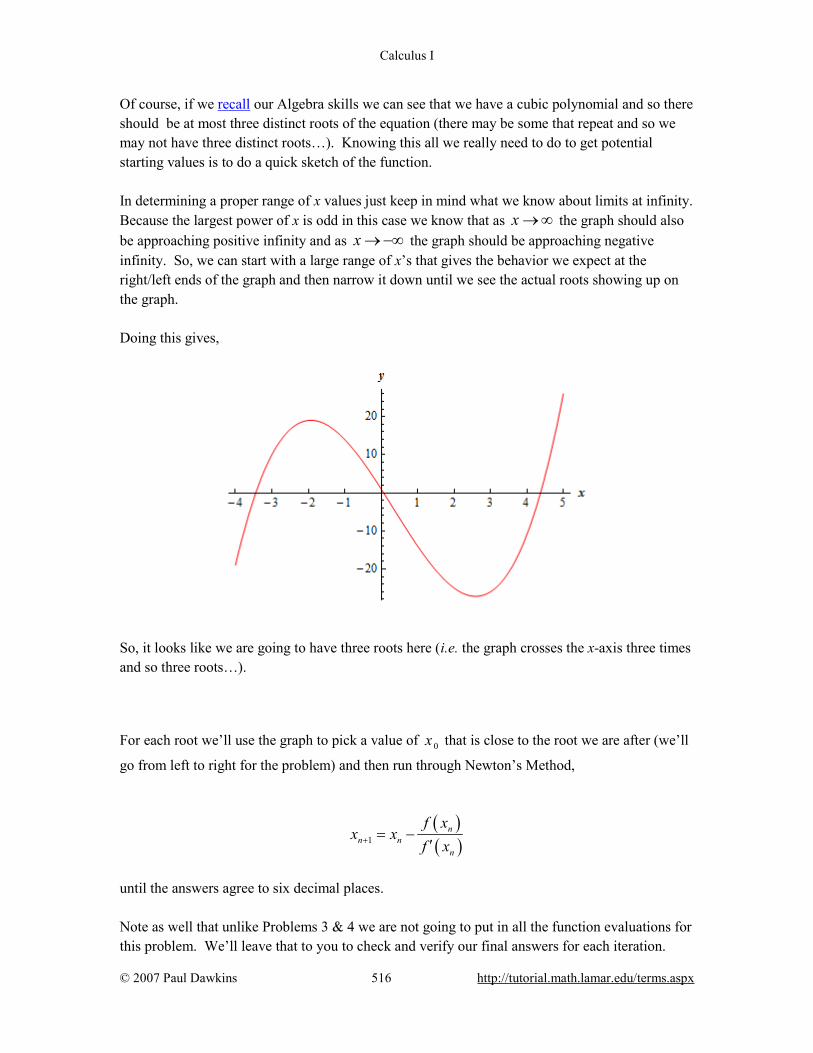
Calculus I
© 2007 Paul Dawkins 516 http://tutorial.math.lamar.edu/terms.aspx
Of course, if we recall our Algebra skills we can see that we have a cubic polynomial and so there should be at most three distinct roots of the equation (there may be some that repeat and so we may not have three distinct roots…). Knowing this all we really need to do to get potential starting values is to do a quick sketch of the function. In determining a proper range of x values just keep in mind what we know about limits at infinity. Because the largest power of x is odd in this case we know that as x → ∞ the graph should also be approaching positive infinity and as x → −∞ the graph should be approaching negative infinity. So, we can start with a large range of x’s that gives the behavior we expect at the right/left ends of the graph and then narrow it down until we see the actual roots showing up on the graph. Doing this gives,
So, it looks like we are going to have three roots here (i.e. the graph crosses the x-axis three times and so three roots…).
For each root we’ll use the graph to pick a value of 0x that is close to the root we are after (we’ll
go from left to right for the problem) and then run through Newton’s Method,
( )( )1
nn n
n
f xx x
f x+ = −′
until the answers agree to six decimal places. Note as well that unlike Problems 3 & 4 we are not going to put in all the function evaluations for this problem. We’ll leave that to you to check and verify our final answers for each iteration.
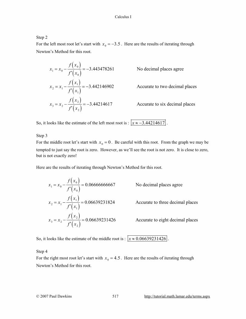
Calculus I
© 2007 Paul Dawkins 517 http://tutorial.math.lamar.edu/terms.aspx
Step 2 For the left most root let’s start with 0 3.5x = − . Here are the results of iterating through
Newton’s Method for this root.
( )( )( )( )( )( )
01 0
0
12 1
1
23 2
2
3.443478261 No decimal places agree
3.442146902 Accurate to two decimal places
3.44214617 Accurate to six decimal places
f xx x
f x
f xx x
f x
f xx x
f x
= − = −′
= − = −′
= − = −′
So, it looks like the estimate of the left most root is : 3.44214617x ≈ − . Step 3 For the middle root let’s start with 0 0x = . Be careful with this root. From the graph we may be
tempted to just say the root is zero. However, as we’ll see the root is not zero. It is close to zero, but is not exactly zero! Here are the results of iterating through Newton’s Method for this root.
( )( )( )( )( )( )
01 0
0
12 1
1
23 2
2
0.06666666667 No decimal places agree
0.06639231824 Accurate to three decimal places
0.06639231426 Accurate to eight decimal places
f xx x
f x
f xx x
f x
f xx x
f x
= − =′
= − =′
= − =′
So, it looks like the estimate of the middle root is : 0.06639231426x ≈ . Step 4 For the right most root let’s start with 0 4.5x = . Here are the results of iterating through
Newton’s Method for this root.
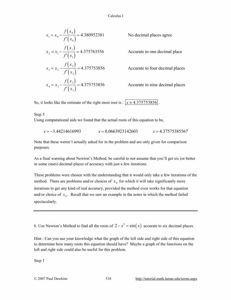
Calculus I
© 2007 Paul Dawkins 518 http://tutorial.math.lamar.edu/terms.aspx
( )( )( )( )( )( )( )( )
01 0
0
12 1
1
23 2
2
34 3
3
4.380952381 No decimal places agree
4.375763556 Accurate to one decimal place
4.375753856 Accurate to four decimal places
4.375753856 Accurate to nine
f xx x
f x
f xx x
f x
f xx x
f x
f xx x
f x
= − =′
= − =′
= − =′
= − =′
decimal places
So, it looks like the estimate of the right most root is : 4.375753856x ≈ . Step 5 Using computational aids we found that the actual roots of this equation to be, 3.44214616993 0.0663923142603 4.37575385567x x x= − = = Note that these weren’t actually asked for in the problem and are only given for comparison purposes. As a final warning about Newton’s Method, be careful to not assume that you’ll get six (or better in some cases) decimal places of accuracy with just a few iterations. These problems were chosen with the understanding that it would only take a few iterations of the method. There are problems and/or choices of 0x for which it will take significantly more
iterations to get any kind of real accuracy, provided the method even works for that equation and/or choice of 0x . Recall that we saw an example in the notes in which the method failed
spectacularly. 6. Use Newton’s Method to find all the roots of ( )22 sinx x− = accurate to six decimal places.
Hint : Can you use your knowledge what the graph of the left side and right side of this equation to determine how many roots this equation should have? Maybe a graph of the functions on the left and right side could also be useful for this problem. Step 1

Calculus I
© 2007 Paul Dawkins 519 http://tutorial.math.lamar.edu/terms.aspx
First, recall that Newton’s Method solves equation in the form ( ) 0f x = and so we’ll need move
everything to one side. Doing this gives, ( ) ( )22 sinf x x x= − − Note that we could have just as easily gone the other direction. All that would have done was change the signs on the function and derivative evaluations in the work below. The final answers however would not be changed. Next, we are not given a starting value, 0x and unlike Problems 3 & 4 above we not even given
an interval to use as a way to determine a good possible value of 0x . We are also not even told
how many roots we need to find. So to estimate the number of roots of the equation let’s take a look at each side of the equation and realize that each root will in fact be the point of intersection of the two curves on the left and right of the equal sign. The left side of the original equation is a quadratic that will have its vertex at 2x = and open downward while the right side is the sine function. Given what we know of these two functions we should expect there to be at most two roots where the quadratic, on its way down, intersects with the sine function. Because the quadratic will never turn around and start moving back upwards it should never intersect with the sine function again after those points. So, let’s graph both the quadratic and sine function to see if our intuition on this is correct. Doing this gives,
So, it looks like we guessed correctly and should have two roots here.

Calculus I
© 2007 Paul Dawkins 520 http://tutorial.math.lamar.edu/terms.aspx
For each root we’ll use the graph to pick a value of 0x that is close to the root we are after (we’ll
go from left to right for the problem) and then run through Newton’s Method,
( )( )1
nn n
n
f xx x
f x+ = −′
until the answers agree to six decimal places. Note as well that unlike Problems 3 & 4 we are not going to put in all the function evaluations for this problem. We’ll leave that to you to check and verify our final answers for each iteration. Also note that the analysis that we had to do to estimate the number of roots is something that does need to be done for these kinds of problems and it will differ for each equation. However, if you do have a basic knowledge of how most of the basic functions behave you can do this for most equations you’ll be asked to deal with. Step 2 For the left most root let’s start with 0 1.5x = − . Here are the results of iterating through
Newton’s Method for this root.
( )( )( )( )( )( )( )( )
01 0
0
12 1
1
23 2
2
34 3
3
1.755181948 No decimal places agree
1.728754674 Accurate to one decimal place
1.728466353 Accurate to three decimal places
1.728466319 Accurate to
f xx x
f x
f xx x
f x
f xx x
f x
f xx x
f x
= − = −′
= − = −′
= − = −′
= − = −′
seven decimal places
So, it looks like the estimate of the left most root is : 1.728466319x ≈ − . Step 3 For the right most root let’s start with 0 1x = . Here are the results of iterating through Newton’s
Method for this root.
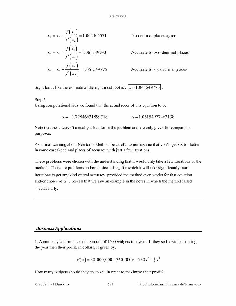
Calculus I
© 2007 Paul Dawkins 521 http://tutorial.math.lamar.edu/terms.aspx
( )( )( )( )( )( )
01 0
0
12 1
1
23 2
2
1.062405571 No decimal places agree
1.061549933 Accurate to two decimal places
1.061549775 Accurate to six decimal places
f xx x
f x
f xx x
f x
f xx x
f x
= − =′
= − =′
= − =′
So, it looks like the estimate of the right most root is : 1.061549775x ≈ . Step 5 Using computational aids we found that the actual roots of this equation to be, 1.72846631899718 1.06154977463138x x= − = Note that these weren’t actually asked for in the problem and are only given for comparison purposes. As a final warning about Newton’s Method, be careful to not assume that you’ll get six (or better in some cases) decimal places of accuracy with just a few iterations. These problems were chosen with the understanding that it would only take a few iterations of the method. There are problems and/or choices of 0x for which it will take significantly more
iterations to get any kind of real accuracy, provided the method even works for that equation and/or choice of 0x . Recall that we saw an example in the notes in which the method failed
spectacularly.
Business Applications 1. A company can produce a maximum of 1500 widgets in a year. If they sell x widgets during the year then their profit, in dollars, is given by, ( ) 2 31
330,000,000 360,000 750P x x x x= − + − How many widgets should they try to sell in order to maximize their profit?
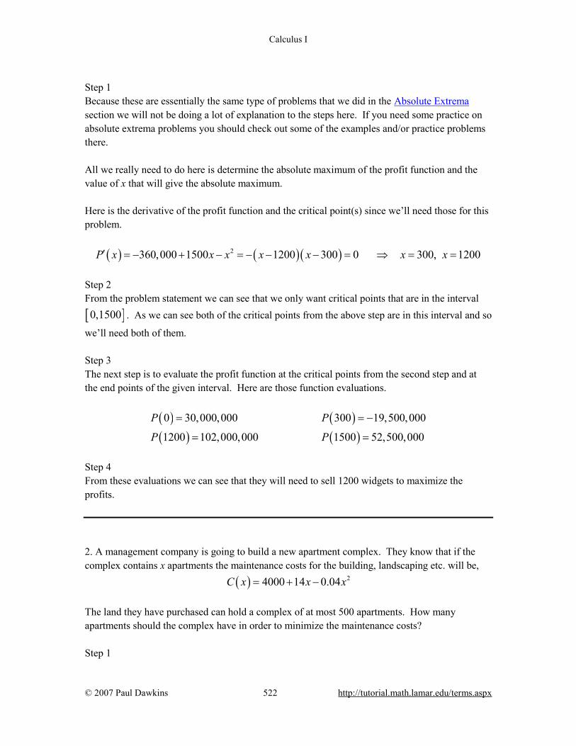
Calculus I
© 2007 Paul Dawkins 522 http://tutorial.math.lamar.edu/terms.aspx
Step 1 Because these are essentially the same type of problems that we did in the Absolute Extrema section we will not be doing a lot of explanation to the steps here. If you need some practice on absolute extrema problems you should check out some of the examples and/or practice problems there. All we really need to do here is determine the absolute maximum of the profit function and the value of x that will give the absolute maximum. Here is the derivative of the profit function and the critical point(s) since we’ll need those for this problem. ( ) ( ) ( )2360,000 1500 1200 300 0 300, 1200P x x x x x x x′ = − + − = − − − = ⇒ = = Step 2 From the problem statement we can see that we only want critical points that are in the interval
[ ]0,1500 . As we can see both of the critical points from the above step are in this interval and so
we’ll need both of them. Step 3 The next step is to evaluate the profit function at the critical points from the second step and at the end points of the given interval. Here are those function evaluations.
( ) ( )( ) ( )0 30,000,000 300 19,500,000
1200 102,000,000 1500 52,500,000
P P
P P
= = −
= =
Step 4 From these evaluations we can see that they will need to sell 1200 widgets to maximize the profits. 2. A management company is going to build a new apartment complex. They know that if the complex contains x apartments the maintenance costs for the building, landscaping etc. will be, ( ) 24000 14 0.04C x x x= + − The land they have purchased can hold a complex of at most 500 apartments. How many apartments should the complex have in order to minimize the maintenance costs? Step 1

Calculus I
© 2007 Paul Dawkins 523 http://tutorial.math.lamar.edu/terms.aspx
Because these are essentially the same type of problems that we did in the Absolute Extrema section we will not be doing a lot of explanation to the steps here. If you need some practice on absolute extrema problems you should check out some of the examples and/or practice problems there. All we really need to do here is determine the absolute minimum of the maintenance function and the value of x that will give the absolute minimum. Here is the derivative of the maintenance function and the critical point(s) since we’ll need those for this problem. ( ) 14 0.08 175C x x x′ = − = ⇒ = Step 2 From the problem statement we can see that we only want critical points that are in the interval
[ ]0,500 . As we can see both of the critical points from the above step are in this interval and so
we’ll need both of them. Step 3 The next step is to evaluate the maintenance function at the critical points from the second step and at the end points of the given interval. Here are those function evaluations. ( ) ( ) ( )0 4000 175 5225 500 1000C C C= = = Step 4 From these evaluations we can see that the complex should have 500 apartments to minimize the maintenance costs. 3. The production costs, in dollars, per day of producing x widgets is given by, ( ) 2 31750 6 0.04 0.0003C x x x x= + − + What is the marginal cost when 175x = and 300x = ? What do your answers tell you about the production costs? Step 1 From the notes in this section we know that the marginal cost is simply the derivative of the cost function so let’s start with that. ( ) 26 0.08 0.0009C x x x′ = − +
Calculus I
© 2007 Paul Dawkins 524 http://tutorial.math.lamar.edu/terms.aspx
Step 2 The marginal costs for each value of x is then,
( ) ( )125 10.0625 300 63C C′ ′= = Step 3 From these computations we can see that is will cost approximately $10.06 to produce the 126th widget and approximately $63 to produce the 301st widget. 4. The production costs, in dollars, per month of producing x widgets is given by,
( ) 10000200 0.5C x xx
= + +
What is the marginal cost when 200x = and 500x = ? What do your answers tell you about the production costs? Step 1 From the notes in this section we know that the marginal cost is simply the derivative of the cost function so let’s start with that.
( ) 2
100000.5C xx
′ = −
Step 2 The marginal costs for each value of x is then,
( ) ( )200 0.25 500 0.46C C′ ′= = Step 3 From these computations we can see that is will cost approximately 25 cents to produce the 201st widget and approximately 46 cents to produce the 501st widget. 5. The production costs, in dollars, per week of producing x widgets is given by, ( ) 2 34000 32 0.08 0.00006C x x x x= − + +
Calculus I
© 2007 Paul Dawkins 525 http://tutorial.math.lamar.edu/terms.aspx
and the demand function for the widgets is given by, ( ) 2250 0.02 0.001p x x x= + − What is the marginal cost, marginal revenue and marginal profit when 200x = and 400x = ? What do these numbers tell you about the cost, revenue and profit? Step 1 First we need to get the revenue and profit functions. From the notes for this section we know that these functions are,
( ) ( )
( ) ( ) ( )
2 3
2 3
Revenue : 250 0.02 0.001
Profit : 4000 282 0.06 0.00106
R x x p x x x x
P x R x C x x x x
= = + −
= − = − + − −
Step 2 From the notes in this section we know that the marginal cost, marginal revenue and marginal profit functions are simply the derivative of the cost, revenue and profit functions so let’s start with those.
( )( )( )
2
2
2
32 0.16 0.00018
250 0.04 0.003
282 0.12 0.00318
C x x x
R x x x
P x x x
′ = − + +
′ = + −
′ = − −
Step 3 The marginal cost, marginal revenue and marginal profit for each value of x is then,
( ) ( ) ( )( ) ( ) ( )200 7.2 200 138 200 130.8
400 60.8 400 214 400 274.8
C R P
C R P
′ ′ ′= = =
′ ′ ′= = − = −
Step 4 From these computations we can see that producing the 201st widget will cost approximately $7.2 and will add approximately $138 in revenue and $130.8 in profit. Likewise, producing the 401st widget will cost approximately $60.8 and will see a decrease of approximately $214 in revenue and a decrease of $274.8 in profit.
Calculus I
© 2007 Paul Dawkins 526 http://tutorial.math.lamar.edu/terms.aspx
Integrals
Indefinite Integrals 1. Evaluate each of the following indefinite integrals.
(a) 5 26 18 7x x dx− +∫
(b) 5 26 18 7x dx x− +∫
Hint : As long as you recall your derivative rules and the fact that all this problem is really asking is the for us to determine the function that we differentiated to get the integrand (i.e. the function inside the integral….) this problem shouldn’t be too difficult.
(a) 5 26 18 7x x dx− +∫
All we are being asked to do here is “undo” a differentiation and if you recall the basic differentiation rules for polynomials this shouldn’t be too difficult. As we saw in the notes for this section all we really need to do is increase the exponent by one (so upon differentiation we get the correct exponent) and then fix up the coefficient to make sure that we will get the correct coefficient upon differentiation. Here is the answer for this part.
5 2 6 36 18 7 6 7x x dx x x x c− + = + + +∫
Don’t forget the “+c”! Remember that the original function may have had a constant on it and the “+c” is there to remind us of that. Also don’t forget that you can easily check your answer by differentiating your answer and making sure that the result is the same as the integrand.
(b) 5 26 18 7x dx x− +∫
This part is not really all that different from the first part. The only difference is the placement of the dx. Recall that one of the things that the dx tells us where to end the integration. So, in the part we are only going to integrate the first term. Here is the answer for this part.
Calculus I
© 2007 Paul Dawkins 527 http://tutorial.math.lamar.edu/terms.aspx
5 2 6 26 18 7 18 7x dx x x c x− + = + − +∫ 2. Evaluate each of the following indefinite integrals.
(a) 3 240 12 9 14x x x dx+ − +∫
(b) 3 240 12 9 14x x x dx+ − +∫
(c) 3 240 12 9 14x x dx x+ − +∫ Hint : As long as you recall your derivative rules and the fact that all this problem is really asking is the for us to determine the function that we differentiated to get the integrand (i.e. the function inside the integral….) this problem shouldn’t be too difficult.
(a) 3 240 12 9 14x x x dx+ − +∫
All we are being asked to do here is “undo” a differentiation and if you recall the basic differentiation rules for polynomials this shouldn’t be too difficult. As we saw in the notes for this section all we really need to do is increase the exponent by one (so upon differentiation we get the correct exponent) and then fix up the coefficient to make sure that we will get the correct coefficient upon differentiation. Here is that answer for this part.
3 2 4 3 29240 12 9 14 10 4 14x x x dx x x x x c+ − + = + − + +∫
Don’t forget the “+c”! Remember that the original function may have had a constant on it and the “+c” is there to remind us of that. Also don’t forget that you can easily check your answer by differentiating your answer and making sure that the result is the same as the integrand.
(b) 3 240 12 9 14x x x dx+ − +∫
This part is not really all that different from the first part. The only difference is the placement of the dx. Recall that one of the things that the dx tells us where to end the integration. So, in the part we are only going to integrate the first term. Here is the answer for this part.
3 2 4 3 29240 12 9 14 10 4 14x x x dx x x x c+ − + = + − + +∫
Calculus I
© 2007 Paul Dawkins 528 http://tutorial.math.lamar.edu/terms.aspx
(c) 3 240 12 9 14x x dx x+ − +∫
The only difference between this part and the previous part is that the location of the dx moved. Here is the answer for this part.
3 2 4 340 12 9 14 10 4 9 14x x dx x x x c x+ − + = + + − +∫
3. Evaluate 7 212 3t t t dt− − +∫ .
Hint : As long as you recall your derivative rules and the fact that all this problem is really asking is the for us to determine the function that we differentiated to get the integrand (i.e. the function inside the integral….) this problem shouldn’t be too difficult. Solution All we are being asked to do here is “undo” a differentiation and if you recall the basic differentiation rules for polynomials this shouldn’t be too difficult. As we saw in the notes for this section all we really need to do is increase the exponent by one (so upon differentiation we get the correct exponent) and then fix up the coefficient to make sure that we will get the correct coefficient upon differentiation. Here is the answer.
7 2 8 3 23 1 12 3 212 3 3t t t dt t t t t c− − + = − − + +∫
Don’t forget the “+c”! Remember that the original function may have had a constant on it and the “+c” is there to remind us of that. Also don’t forget that you can easily check your answer by differentiating your answer and making sure that the result is the same as the integrand.
4. Evaluate 4 310 9 7w w w dw+ +∫ .
Hint : As long as you recall your derivative rules and the fact that all this problem is really asking is the for us to determine the function that we differentiated to get the integrand (i.e. the function inside the integral….) this problem shouldn’t be too difficult.
Calculus I
© 2007 Paul Dawkins 529 http://tutorial.math.lamar.edu/terms.aspx
Solution All we are being asked to do here is “undo” a differentiation and if you recall the basic differentiation rules for polynomials this shouldn’t be too difficult. As we saw in the notes for this section all we really need to do is increase the exponent by one (so upon differentiation we get the correct exponent) and then fix up the coefficient to make sure that we will get the correct coefficient upon differentiation. Here is the answer.
4 3 5 4 29 74 210 9 7 2w w w dw w w w c+ + = + + +∫
Don’t forget the “+c”! Remember that the original function may have had a constant on it and the “+c” is there to remind us of that. Also don’t forget that you can easily check your answer by differentiating your answer and making sure that the result is the same as the integrand.
5. Evaluate 6 4 24z z z dz+ −∫ .
Hint : As long as you recall your derivative rules and the fact that all this problem is really asking is the for us to determine the function that we differentiated to get the integrand (i.e. the function inside the integral….) this problem shouldn’t be too difficult. Solution All we are being asked to do here is “undo” a differentiation and if you recall the basic differentiation rules for polynomials this shouldn’t be too difficult. As we saw in the notes for this section all we really need to do is increase the exponent by one (so upon differentiation we get the correct exponent) and then fix up the coefficient to make sure that we will get the correct coefficient upon differentiation. Here is the answer.
6 4 2 7 5 31 4 17 5 34z z z dz z z z c+ − = + − +∫
Don’t forget the “+c”! Remember that the original function may have had a constant on it and the “+c” is there to remind us of that. Also don’t forget that you can easily check your answer by differentiating your answer and making sure that the result is the same as the integrand.
Calculus I
© 2007 Paul Dawkins 530 http://tutorial.math.lamar.edu/terms.aspx
6. Determine ( )f x given that ( ) 8 4 26 20 9f x x x x′ = − + + .
Hint : Remember that all indefinite integrals are asking us to do is “undo” a differentiation. Solution We know that indefinite integrals are asking us to undo a differentiation to so all we are really being asked to do here is evaluate the following indefinite integral.
( ) ( ) 8 4 2 9 5 32 13 36 20 9 4 9f x f x dx x x x dx x x x x c′= = − + + = − + + +∫ ∫
Don’t forget the “+c”! Remember that the original function may have had a constant on it and the “+c” is there to remind us of that. 7. Determine ( )h t given that ( ) 4 3 2 1h t t t t t′ = − + + − .
Hint : Remember that all indefinite integrals are asking us to do is “undo” a differentiation. Solution We know that indefinite integrals are asking us to undo a differentiation to so all we are really being asked to do here is evaluate the following indefinite integral.
( ) ( ) 4 3 2 5 4 3 21 1 1 15 4 3 21h t h t dt t t t t dt t t t t t c′= = − + + − = − + + − +∫ ∫
Don’t forget the “+c”! Remember that the original function may have had a constant on it and the “+c” is there to remind us of that.
Computing Indefinite Integrals
1. Evaluate 6 34 2 7 4x x x dx− + −∫ .
Solution There really isn’t too much to do other than to evaluate the integral.
Calculus I
© 2007 Paul Dawkins 531 http://tutorial.math.lamar.edu/terms.aspx
6 3 7 4 2 7 4 27 74 2 4 17 4 2 7 2 24 2 7 4 4 4x x x dx x x x x c x x x x c− + − = − + − + = − + − +∫
Don’t forget to add on the “+c” since we know that we are asking what function did we differentiate to get the integrand and the derivative of a constant is zero and so we do need to add that onto the answer.
2. Evaluate 7 11 1648 5z z z dz− −∫ .
Solution There really isn’t too much to do other than to evaluate the integral.
7 11 16 8 12 17 8 12 1748 5 51 18 12 17 8 1748 5 4z z z dz z z z c z z z c− − = − − + = − − +∫
Don’t forget to add on the “+c” since we know that we are asking what function did we differentiate to get the integrand and the derivative of a constant is zero and so we do need to add that onto the answer.
3. Evaluate 3 9 310 12 4t t t dt− −+ +∫ .
Solution There really isn’t too much to do other than to evaluate the integral.
3 9 3 2 8 4 2 8 410 312 42 8 4 210 12 4 5t t t dt t t t c t t t c− − − − − −
− −+ + = + + + = − − + +∫ Don’t forget to add on the “+c” since we know that we are asking what function did we differentiate to get the integrand and the derivative of a constant is zero and so we do need to add that onto the answer.
4. Evaluate 2 510 8w w dw− −+ −∫ .
Solution There really isn’t too much to do other than to evaluate the integral.
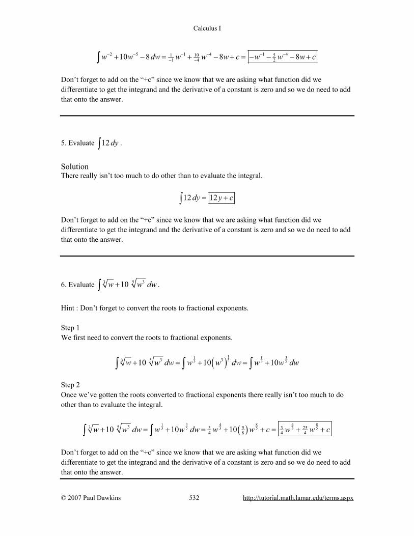
Calculus I
© 2007 Paul Dawkins 532 http://tutorial.math.lamar.edu/terms.aspx
2 5 1 4 1 410 511 4 210 8 8 8w w dw w w w c w w w c− − − − − −
− −+ − = + − + = − − − +∫ Don’t forget to add on the “+c” since we know that we are asking what function did we differentiate to get the integrand and the derivative of a constant is zero and so we do need to add that onto the answer.
5. Evaluate 12 dy∫ .
Solution There really isn’t too much to do other than to evaluate the integral.
12 12dy y c= +∫ Don’t forget to add on the “+c” since we know that we are asking what function did we differentiate to get the integrand and the derivative of a constant is zero and so we do need to add that onto the answer.
6. Evaluate 5 33 10w w dw+∫ .
Hint : Don’t forget to convert the roots to fractional exponents. Step 1 We first need to convert the roots to fractional exponents.
( )11 1 353 3 55 3 33 10 10 10w w dw w w dw w w dw+ = + = +∫ ∫ ∫
Step 2 Once we’ve gotten the roots converted to fractional exponents there really isn’t too much to do other than to evaluate the integral.
( )1 3 4 8 4 83 5 3 5 3 55 33 3 5 3 25
4 8 4 410 10 10w w dw w w dw w w c w w c+ = + = + + = + +∫ ∫ Don’t forget to add on the “+c” since we know that we are asking what function did we differentiate to get the integrand and the derivative of a constant is zero and so we do need to add that onto the answer.

Calculus I
© 2007 Paul Dawkins 533 http://tutorial.math.lamar.edu/terms.aspx
7. Evaluate 6 37 5 107 17x x x dx− +∫ .
Hint : Don’t forget to convert the roots to fractional exponents. Step 1 We first need to convert the roots to fractional exponents.
( ) ( )1 1 5 107 76 3 6 32 26 37 5 10 5 107 17 7 17 7 17x x x dx x x x dx x x x dx− + = − + = − +∫ ∫ ∫
Step 2 Once we’ve gotten the roots converted to fractional exponents there really isn’t too much to do other than to evaluate the integral.
( ) ( )
5 1076 32
13 139 11 9 116 3 6 32 2
6 37 5 10
6 3 512 2 429 11 13 9 11 13
7 17 7 17
7 17
x x x dx x x x dx
x x x c x x x c
− + = − +
= − + + = − + +
∫ ∫
Don’t forget to add on the “+c” since we know that we are asking what function did we differentiate to get the integrand and the derivative of a constant is zero and so we do need to add that onto the answer.
8. Evaluate 2 3
4 128
dxx x
+ −⌠⌡
.
Hint : Don’t forget to move the x’s in the denominator to the numerator with negative exponents. Step 1 We first need to move the x’s in the denominator to the numerator with negative exponents.
2 32 3
4 1 12 4 28 8
dx x x dxx x
− −+ − = + −⌠ ⌠ ⌡ ⌡
Remember that the “8” in the denominator of the third term stays in the denominator and does not move up with the x. Step 2
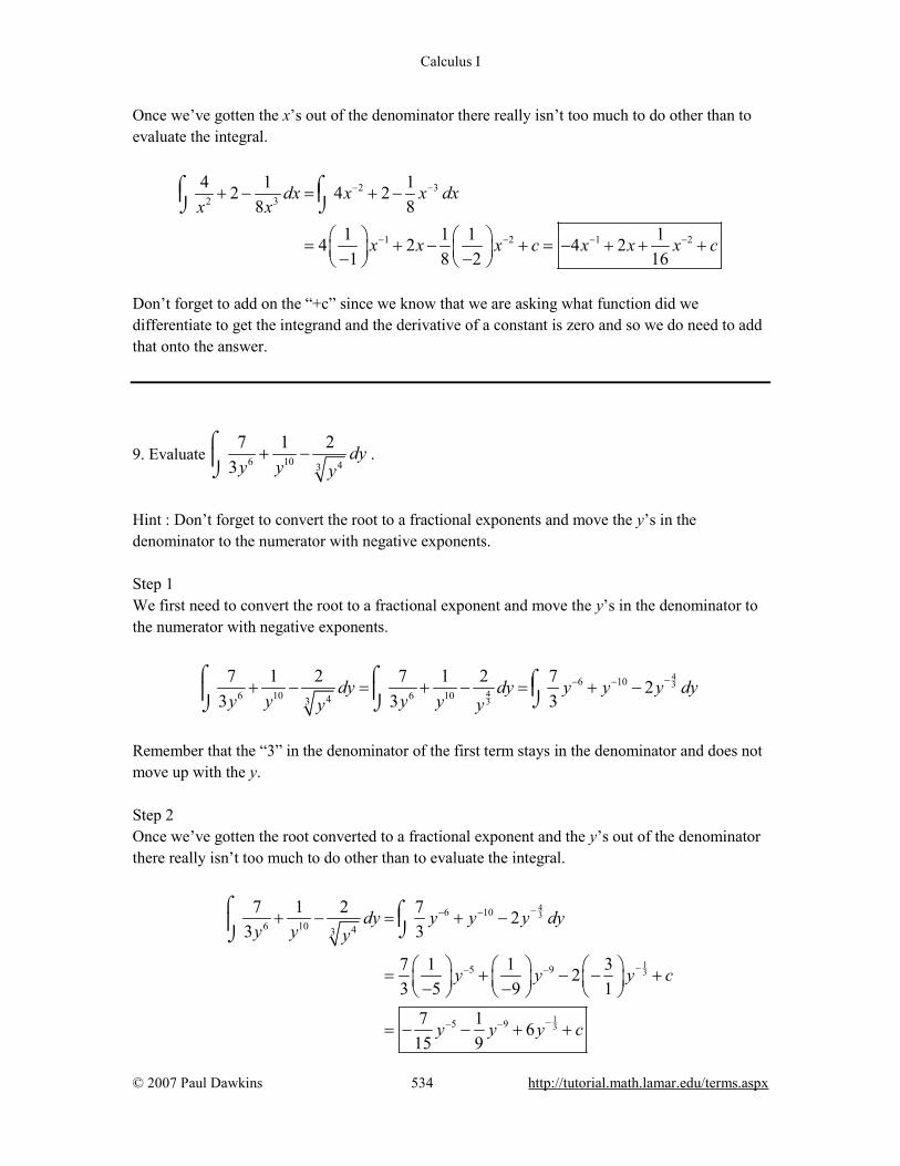
Calculus I
© 2007 Paul Dawkins 534 http://tutorial.math.lamar.edu/terms.aspx
Once we’ve gotten the x’s out of the denominator there really isn’t too much to do other than to evaluate the integral.
2 32 3
1 2 1 2
4 1 12 4 28 8
1 1 1 14 2 4 21 8 2 16
dx x x dxx x
x x x c x x x c
− −
− − − −
+ − = + −
= + − + = − + + + − −
⌠ ⌠ ⌡ ⌡
Don’t forget to add on the “+c” since we know that we are asking what function did we differentiate to get the integrand and the derivative of a constant is zero and so we do need to add that onto the answer.
9. Evaluate 6 10 43
7 1 23
dyy y y
+ −⌠⌡
.
Hint : Don’t forget to convert the root to a fractional exponents and move the y’s in the denominator to the numerator with negative exponents. Step 1 We first need to convert the root to a fractional exponent and move the y’s in the denominator to the numerator with negative exponents.
43
43
6 106 10 6 1043
7 1 2 7 1 2 7 23 3 3
dy dy y y y dyy y y y yy
−− −+ − = + − = + −⌠ ⌠ ⌠ ⌡⌡⌡
Remember that the “3” in the denominator of the first term stays in the denominator and does not move up with the y. Step 2 Once we’ve gotten the root converted to a fractional exponent and the y’s out of the denominator there really isn’t too much to do other than to evaluate the integral.
43
13
13
6 106 10 43
5 9
5 9
7 1 2 7 23 3
7 1 1 323 5 9 1
7 1 615 9
dy y y y dyy y y
y y y c
y y y c
−− −
−− −
−− −
+ − = + −
= + − − + − −
= − − + +
⌠ ⌠ ⌡⌡

Calculus I
© 2007 Paul Dawkins 535 http://tutorial.math.lamar.edu/terms.aspx
Don’t forget to add on the “+c” since we know that we are asking what function did we differentiate to get the integrand and the derivative of a constant is zero and so we do need to add that onto the answer.
10. Evaluate ( )( )2 1 4 3t t dt− +∫ .
Hint : Remember that there is no “Product Rule” for integrals and so we’ll need to eliminate the product before integrating. Step 1 Since there is no “Product Rule” for integrals we’ll need to multiply the terms out prior to integration.
( )( )2 3 21 4 3 3 4 3 4t t dt t t t dt− + = + − −∫ ∫ Step 2 At this point there really isn’t too much to do other than to evaluate the integral.
( )( )2 3 2 4 3 23 344 3 21 4 3 3 4 3 4 4t t dt t t t dt t t t t c− + = + − − = + − − +∫ ∫
Don’t forget to add on the “+c” since we know that we are asking what function did we differentiate to get the integrand and the derivative of a constant is zero and so we do need to add that onto the answer.
11. Evaluate 2 14
z z dzz
−
⌠⌡
.
Hint : Remember that there is no “Product Rule” for integrals and so we’ll need to eliminate the product before integrating. Step 1 Since there is no “Product Rule” for integrals we’ll need to multiply the terms out prior to integration.
5 5 12 2 2
12
2 1 1 14 44
z z dz z dz z z dzz z
− − = − = −
⌠⌠ ⌠ ⌡⌡ ⌡
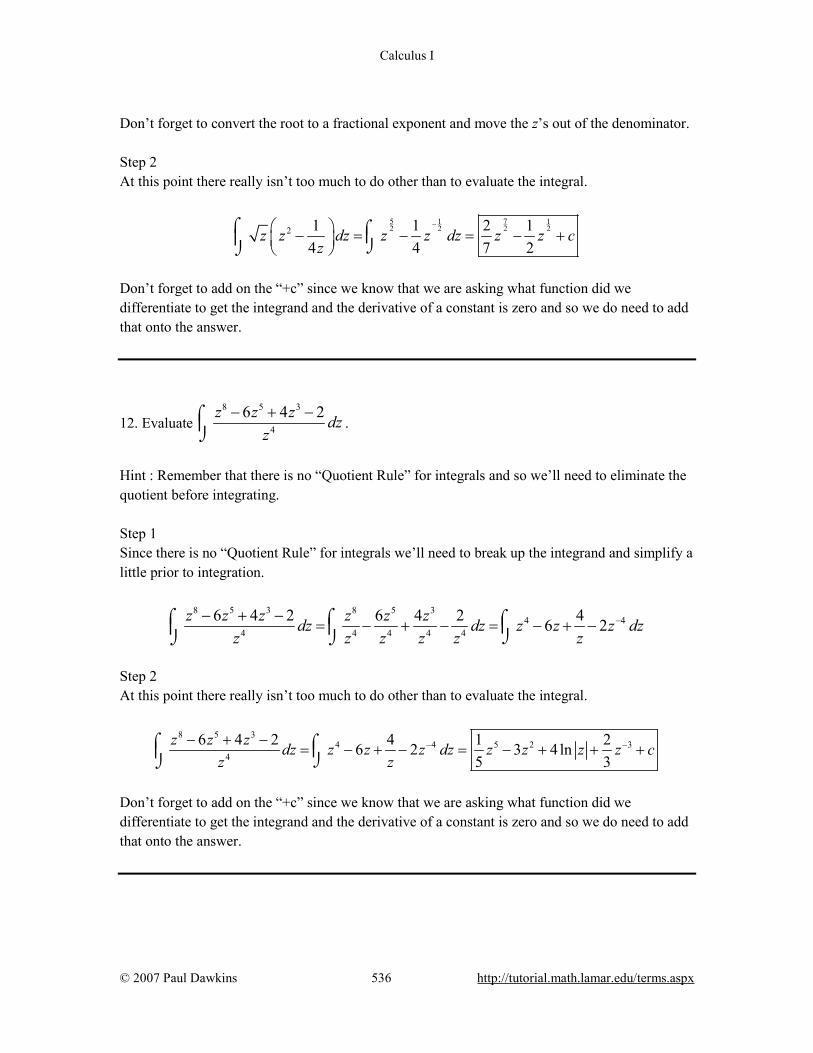
Calculus I
© 2007 Paul Dawkins 536 http://tutorial.math.lamar.edu/terms.aspx
Don’t forget to convert the root to a fractional exponent and move the z’s out of the denominator. Step 2 At this point there really isn’t too much to do other than to evaluate the integral.
5 71 12 2 2 22 1 1 2 1
4 4 7 2z z dz z z dz z z c
z
− − = − = − +
⌠ ⌠ ⌡⌡
Don’t forget to add on the “+c” since we know that we are asking what function did we differentiate to get the integrand and the derivative of a constant is zero and so we do need to add that onto the answer.
12. Evaluate 8 5 3
4
6 4 2z z z dzz
− + −⌠⌡
.
Hint : Remember that there is no “Quotient Rule” for integrals and so we’ll need to eliminate the quotient before integrating. Step 1 Since there is no “Quotient Rule” for integrals we’ll need to break up the integrand and simplify a little prior to integration.
8 5 3 8 5 3
4 44 4 4 4 4
6 4 2 6 4 2 46 2z z z z z zdz dz z z z dzz z z z z z
−− + −= − + − = − + −⌠ ⌠ ⌠ ⌡⌡ ⌡
Step 2 At this point there really isn’t too much to do other than to evaluate the integral.
8 5 3
4 4 5 2 34
6 4 2 4 1 26 2 3 4ln5 3
z z z dz z z z dz z z z z cz z
− −− + −= − + − = − + + +⌠ ⌠ ⌡⌡
Don’t forget to add on the “+c” since we know that we are asking what function did we differentiate to get the integrand and the derivative of a constant is zero and so we do need to add that onto the answer.
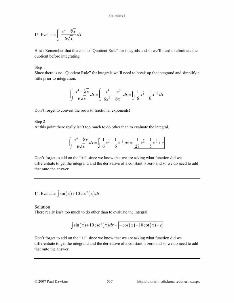
Calculus I
© 2007 Paul Dawkins 537 http://tutorial.math.lamar.edu/terms.aspx
13. Evaluate 4 3
6x x dx
x−⌠
⌡
.
Hint : Remember that there is no “Quotient Rule” for integrals and so we’ll need to eliminate the quotient before integrating. Step 1 Since there is no “Quotient Rule” for integrals we’ll need to break up the integrand and simplify a little prior to integration.
13 7 1
621 12 2
4 43 1 16 66 6 6
x x x xdx dx x x dxx x x
−−= − = −
⌠⌠ ⌠ ⌡⌡ ⌡ Don’t forget to convert the roots to fractional exponents! Step 2 At this point there really isn’t too much to do other than to evaluate the integral.
57 1 9
6 62 24 3 1 1 1 1
6 6 27 56x x dx x x dx x x c
x−−
= − = − +⌠ ⌠ ⌡⌡
Don’t forget to add on the “+c” since we know that we are asking what function did we differentiate to get the integrand and the derivative of a constant is zero and so we do need to add that onto the answer.
14. Evaluate ( ) ( )2sin 10cscx x dx+∫ .
Solution There really isn’t too much to do other than to evaluate the integral.
( ) ( ) ( ) ( )2sin 10csc cos 10cotx x dx x x c+ = − − +∫ Don’t forget to add on the “+c” since we know that we are asking what function did we differentiate to get the integrand and the derivative of a constant is zero and so we do need to add that onto the answer.

Calculus I
© 2007 Paul Dawkins 538 http://tutorial.math.lamar.edu/terms.aspx
15. Evaluate ( ) ( ) ( )2cos sec tanw w w dw−∫ .
Solution There really isn’t too much to do other than to evaluate the integral.
( ) ( ) ( ) ( ) ( )2cos sec tan 2sin secw w w dw w w c− = − +∫ Don’t forget to add on the “+c” since we know that we are asking what function did we differentiate to get the integrand and the derivative of a constant is zero and so we do need to add that onto the answer.
16. Evaluate ( ) ( ) ( )12 csc sin csc dθ θ θ θ+ + ∫ .
Hint : From previous problems in this set we should know how to deal with the product in the integrand. Step 1 Before doing the integral we need to multiply out the product and don’t forget the definition of cosecant in terms of sine.
( ) ( ) ( ) ( ) ( ) ( )
( )
2
2
12 csc sin csc 12 csc sin csc
13 csc
d d
d
θ θ θ θ θ θ θ θ
θ θ
+ + = + +
= +
∫ ∫∫
Recall that,
( ) ( )1csc
sinθ
θ=
and so, ( ) ( )csc sin 1θ θ = Doing this allows us to greatly simplify the integrand and, in fact, allows us to actually do the integral. Without this simplification we would not have been able to integrate the second term with the knowledge that we currently have. Step 2 At this point there really isn’t too much to do other than to evaluate the integral.
( ) ( ) ( ) ( ) ( )212 csc sin csc 13 csc 13 cotd d cθ θ θ θ θ θ θ θ+ + = + = − + ∫ ∫

Calculus I
© 2007 Paul Dawkins 539 http://tutorial.math.lamar.edu/terms.aspx
Don’t forget that with trig functions some terms can be greatly simplified just by recalling the definition of the trig functions and/or their relationship with the other trig functions.
17. Evaluate 14 156
z dzz
+ −⌠⌡
e .
Solution There really isn’t too much to do other than to evaluate the integral.
1 1 1 14 15 4 15 4 15 ln6 6 6
z z zdz dz z z cz z
+ − = + − = + − +⌠ ⌠ ⌡ ⌡
e e e
Be careful with the “6” in the denominator of the third term. The “best” way of dealing with it in this case is to split up the third term as we’ve done above and then integrate. Note that the “best” way to do a problem is always relative for many Calculus problems. There are other ways of dealing with this term (later section material) and so what one person finds the best another may not. For us, this seems to be an easy way to deal with the 6 and not overly complicate the integration process.
18. Evaluate 3 4t
tt dt−
−−
−⌠⌡
ee
.
Hint : From previous problems in this set we should know how to deal with the quotient in the integrand. Step 1 Before doing the integral we need to break up the quotient and do some simplification.
3 3 34 4 1 4t t
tt t tt dt t dt t dt
− −
− − −−
− = − + = − +⌠ ⌠ ⌡ ⌡ ∫
e e ee e e
Make sure that you correctly distribute the minus sign when breaking up the second term and don’t forget to move the exponential in the denominator of the third term (after splitting up the integrand) to the numerator and changing the sign on the t to a “+” in the process. Step 2

Calculus I
© 2007 Paul Dawkins 540 http://tutorial.math.lamar.edu/terms.aspx
At this point there really isn’t too much to do other than to evaluate the integral.
3 3 44 11 4 44
tt t
tt dt t dt t t c−
−−
− = − + = − + +⌠⌡ ∫
e e ee
19. Evaluate 3
6 2 dww w
−⌠⌡
.
Solution There really isn’t too much to do other than to evaluate the integral.
3 23
6 2 26 3 2lndw w dw w w cw w w
− −− = − = − − +⌠ ⌠ ⌡ ⌡
20. Evaluate 2 2
1 121 1
dxx x
++ −
⌠⌡
.
Solution There really isn’t too much to do other than to evaluate the integral.
( ) ( )1 12 2
1 12 tan 12sin1 1
dx x x cx x
− −+ = + ++ −
⌠⌡
Note that because of the similarity of the derivative of inverse sine and inverse cosine an alternate answer is,
( ) ( )1 12 2
1 12 tan 12cos1 1
dx x x cx x
− −+ = − ++ −
⌠⌡
21. Evaluate ( )2
46cos1
z dzz
+−
∫ .
Solution There really isn’t too much to do other than to evaluate the integral.
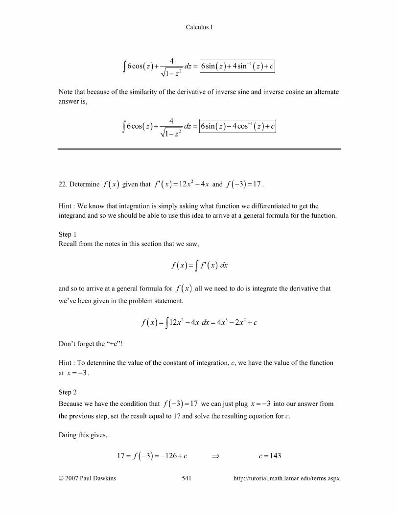
Calculus I
© 2007 Paul Dawkins 541 http://tutorial.math.lamar.edu/terms.aspx
( ) ( ) ( )1
2
46cos 6sin 4sin1
z dz z z cz
−+ = + +−
∫
Note that because of the similarity of the derivative of inverse sine and inverse cosine an alternate answer is,
( ) ( ) ( )1
2
46cos 6sin 4cos1
z dz z z cz
−+ = − +−
∫
22. Determine ( )f x given that ( ) 212 4f x x x′ = − and ( )3 17f − = .
Hint : We know that integration is simply asking what function we differentiated to get the integrand and so we should be able to use this idea to arrive at a general formula for the function. Step 1 Recall from the notes in this section that we saw,
( ) ( )f x f x dx′= ∫ and so to arrive at a general formula for ( )f x all we need to do is integrate the derivative that
we’ve been given in the problem statement.
( ) 2 3 212 4 4 2f x x x dx x x c= − = − +∫
Don’t forget the “+c”! Hint : To determine the value of the constant of integration, c, we have the value of the function at 3x = − . Step 2 Because we have the condition that ( )3 17f − = we can just plug 3x = − into our answer from
the previous step, set the result equal to 17 and solve the resulting equation for c. Doing this gives, ( )17 3 126 143f c c= − = − + ⇒ =

Calculus I
© 2007 Paul Dawkins 542 http://tutorial.math.lamar.edu/terms.aspx
The function is then,
( ) 3 24 2 143f x x x= − +
23. Determine ( )g z given that ( ) 3 732
zg z zz
′ = + − e and ( )1 15g = − e .
Hint : We know that integration is simply asking what function we differentiated to get the integrand and so we should be able to use this idea to arrive at a general formula for the function. Step 1 Recall from the notes in this section that we saw,
( ) ( )g z g z dz′= ∫ and so to arrive at a general formula for ( )g z all we need to do is integrate the derivative that
we’ve been given in the problem statement.
( ) 1 12 23 47 3
2 43 7z zg z z z dz z z c−= + − = + − +∫ e e
Don’t forget the “+c”! Hint : To determine the value of the constant of integration, c, we have the value of the function at 1z = . Step 2 Because we have the condition that ( )1 15g = − e we can just plug 1z = into our answer from
the previous step, set the result equal to 15 – e and solve the resulting equation for c. Doing this gives, ( ) 31 29
4 415 1g c c− = = − + ⇒ =e e
The function is then,
( ) 1243 29
4 47 zg z z z= + − +e
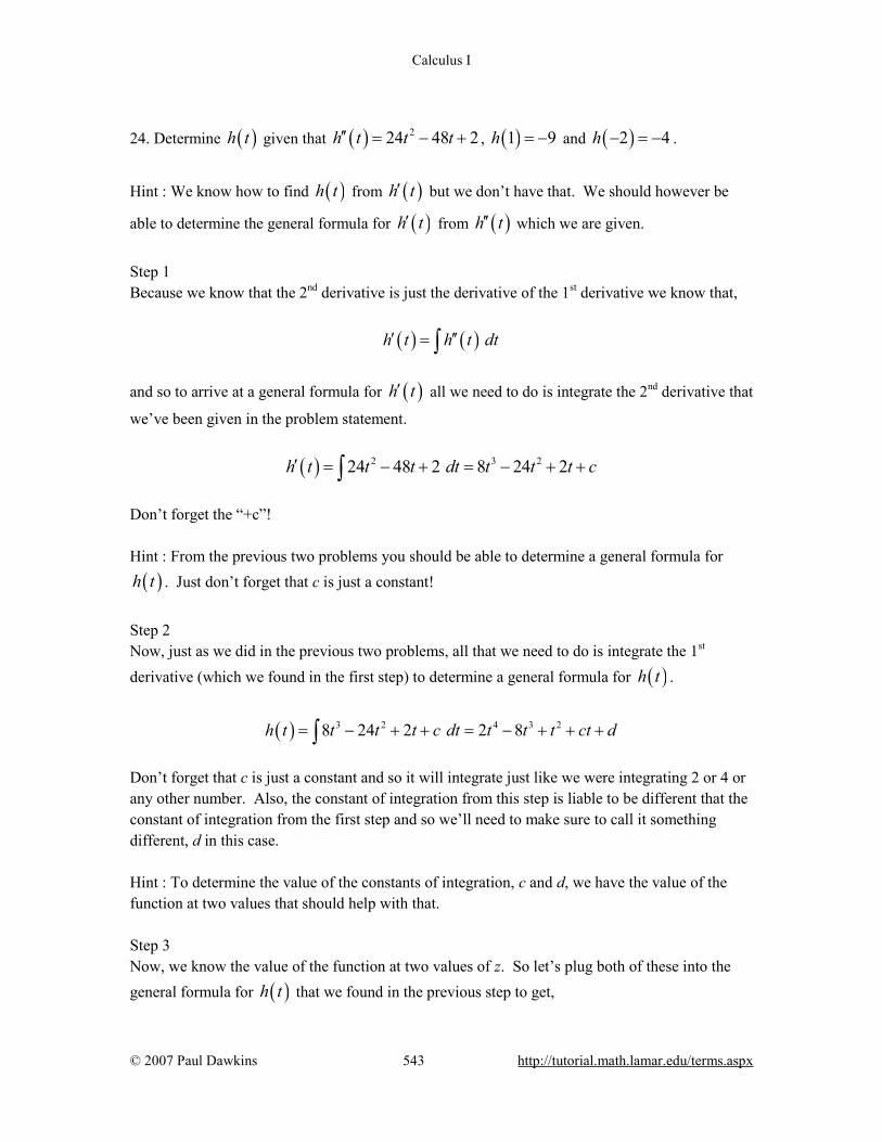
Calculus I
© 2007 Paul Dawkins 543 http://tutorial.math.lamar.edu/terms.aspx
24. Determine ( )h t given that ( ) 224 48 2h t t t′′ = − + , ( )1 9h = − and ( )2 4h − = − .
Hint : We know how to find ( )h t from ( )h t′ but we don’t have that. We should however be
able to determine the general formula for ( )h t′ from ( )h t′′ which we are given.
Step 1 Because we know that the 2nd derivative is just the derivative of the 1st derivative we know that,
( ) ( )h t h t dt′ ′′= ∫ and so to arrive at a general formula for ( )h t′ all we need to do is integrate the 2nd derivative that
we’ve been given in the problem statement.
( ) 2 3 224 48 2 8 24 2h t t t dt t t t c′ = − + = − + +∫
Don’t forget the “+c”! Hint : From the previous two problems you should be able to determine a general formula for
( )h t . Just don’t forget that c is just a constant!
Step 2 Now, just as we did in the previous two problems, all that we need to do is integrate the 1st derivative (which we found in the first step) to determine a general formula for ( )h t .
( ) 3 2 4 3 28 24 2 2 8h t t t t c dt t t t ct d= − + + = − + + +∫ Don’t forget that c is just a constant and so it will integrate just like we were integrating 2 or 4 or any other number. Also, the constant of integration from this step is liable to be different that the constant of integration from the first step and so we’ll need to make sure to call it something different, d in this case. Hint : To determine the value of the constants of integration, c and d, we have the value of the function at two values that should help with that. Step 3 Now, we know the value of the function at two values of z. So let’s plug both of these into the general formula for ( )h t that we found in the previous step to get,
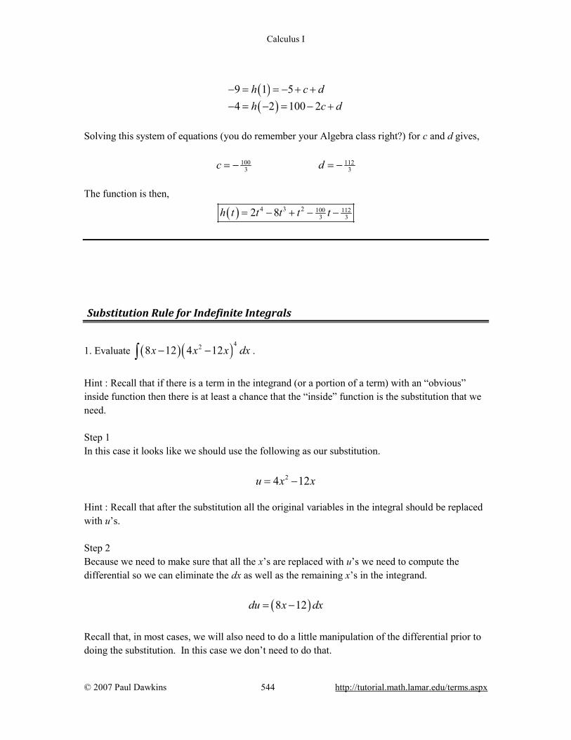
Calculus I
© 2007 Paul Dawkins 544 http://tutorial.math.lamar.edu/terms.aspx
( )( )
9 1 54 2 100 2
h c dh c d
− = = − + +− = − = − +
Solving this system of equations (you do remember your Algebra class right?) for c and d gives, 100 112
3 3c d= − = −
The function is then,
( ) 4 3 2 100 1123 32 8h t t t t t= − + − −
Substitution Rule for Indefinite Integrals
1. Evaluate ( )( )428 12 4 12x x x dx− −∫ .
Hint : Recall that if there is a term in the integrand (or a portion of a term) with an “obvious” inside function then there is at least a chance that the “inside” function is the substitution that we need. Step 1 In this case it looks like we should use the following as our substitution. 24 12u x x= − Hint : Recall that after the substitution all the original variables in the integral should be replaced with u’s. Step 2 Because we need to make sure that all the x’s are replaced with u’s we need to compute the differential so we can eliminate the dx as well as the remaining x’s in the integrand.
( )8 12du x dx= −
Recall that, in most cases, we will also need to do a little manipulation of the differential prior to doing the substitution. In this case we don’t need to do that.
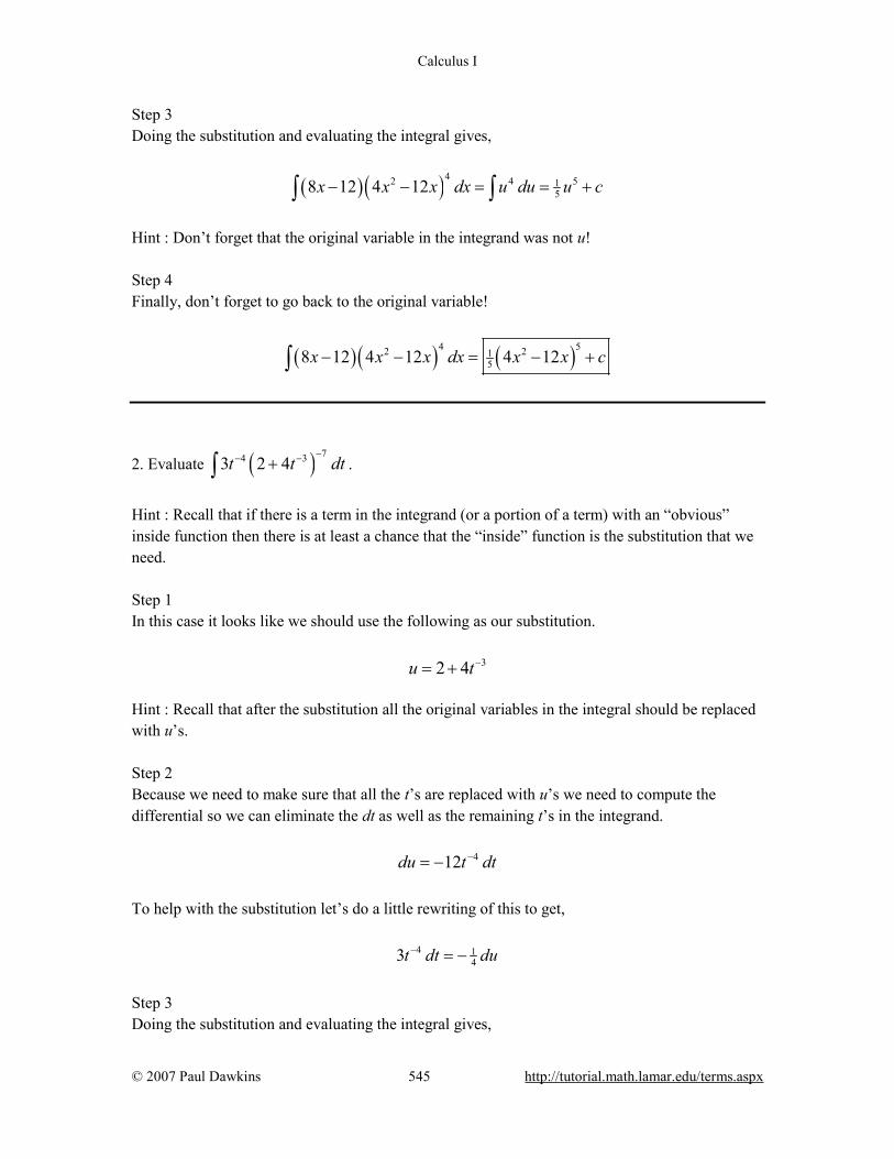
Calculus I
© 2007 Paul Dawkins 545 http://tutorial.math.lamar.edu/terms.aspx
Step 3 Doing the substitution and evaluating the integral gives,
( ) ( )42 4 5158 12 4 12x x x dx u du u c− − = = +∫ ∫
Hint : Don’t forget that the original variable in the integrand was not u! Step 4 Finally, don’t forget to go back to the original variable!
( ) ( ) ( )4 52 2158 12 4 12 4 12x x x dx x x c− − = − +∫
2. Evaluate ( ) 74 33 2 4t t dt−− −+∫ .
Hint : Recall that if there is a term in the integrand (or a portion of a term) with an “obvious” inside function then there is at least a chance that the “inside” function is the substitution that we need. Step 1 In this case it looks like we should use the following as our substitution. 32 4u t−= + Hint : Recall that after the substitution all the original variables in the integral should be replaced with u’s. Step 2 Because we need to make sure that all the t’s are replaced with u’s we need to compute the differential so we can eliminate the dt as well as the remaining t’s in the integrand.
412du t dt−= − To help with the substitution let’s do a little rewriting of this to get,
4 143t dt du− = −
Step 3 Doing the substitution and evaluating the integral gives,
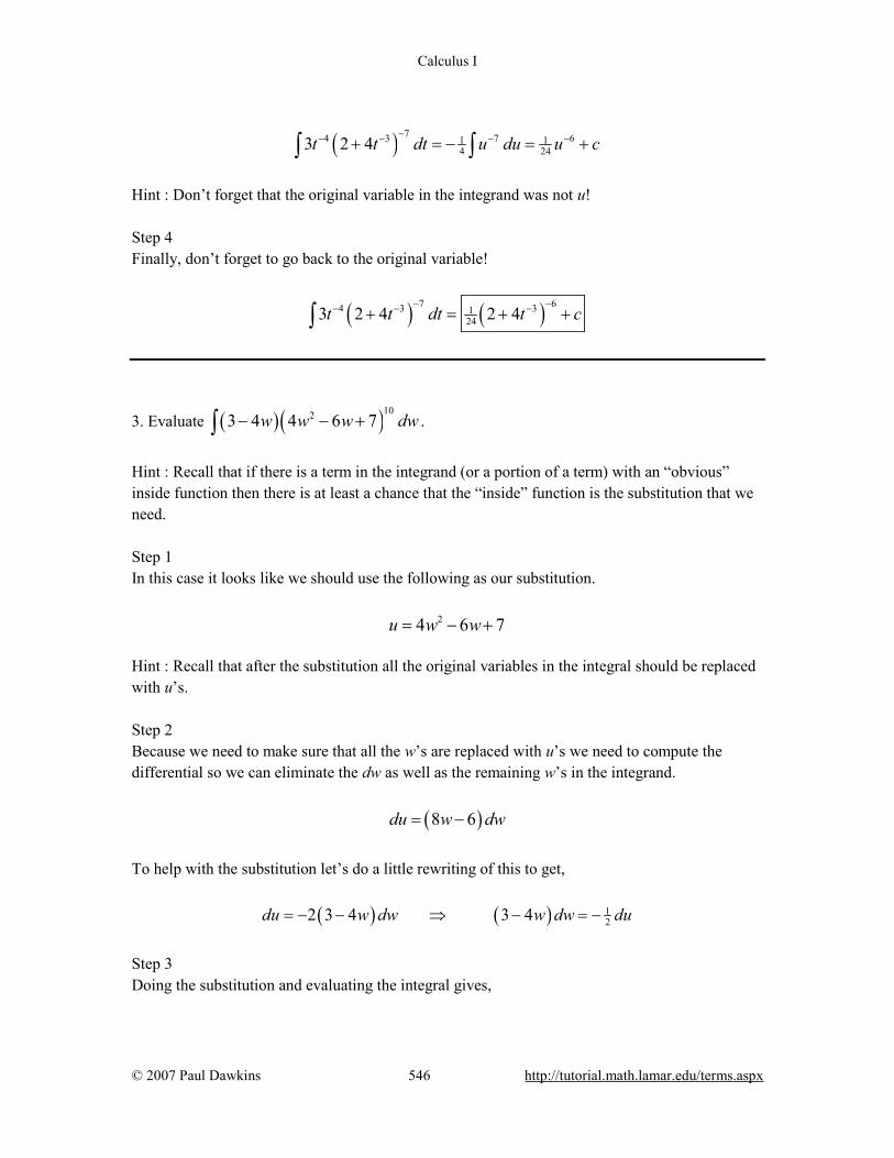
Calculus I
© 2007 Paul Dawkins 546 http://tutorial.math.lamar.edu/terms.aspx
( ) 74 3 7 61 14 243 2 4t t dt u du u c
−− − − −+ = − = +∫ ∫
Hint : Don’t forget that the original variable in the integrand was not u! Step 4 Finally, don’t forget to go back to the original variable!
( ) ( )7 64 3 31243 2 4 2 4t t dt t c
− −− − −+ = + +∫
3. Evaluate ( )( )1023 4 4 6 7w w w dw− − +∫ .
Hint : Recall that if there is a term in the integrand (or a portion of a term) with an “obvious” inside function then there is at least a chance that the “inside” function is the substitution that we need. Step 1 In this case it looks like we should use the following as our substitution. 24 6 7u w w= − + Hint : Recall that after the substitution all the original variables in the integral should be replaced with u’s. Step 2 Because we need to make sure that all the w’s are replaced with u’s we need to compute the differential so we can eliminate the dw as well as the remaining w’s in the integrand.
( )8 6du w dw= −
To help with the substitution let’s do a little rewriting of this to get,
( ) ( ) 122 3 4 3 4du w dw w dw du= − − ⇒ − = −
Step 3 Doing the substitution and evaluating the integral gives,

Calculus I
© 2007 Paul Dawkins 547 http://tutorial.math.lamar.edu/terms.aspx
( ) ( )102 10 111 12 223 4 4 6 7w w w dw u du u c− − + = − = − +∫ ∫
Hint : Don’t forget that the original variable in the integrand was not u! Step 4 Finally, don’t forget to go back to the original variable!
( ) ( ) ( )10 112 21223 4 4 6 7 4 6 7w w w dw w w c− − + = − − + +∫
4. Evaluate ( ) 3 25 4 8z z z dz− −∫ .
Hint : Recall that if there is a term in the integrand (or a portion of a term) with an “obvious” inside function then there is at least a chance that the “inside” function is the substitution that we need. Step 1 In this case it looks like we should use the following as our substitution. 2 8u z z= − Hint : Recall that after the substitution all the original variables in the integral should be replaced with u’s. Step 2 Because we need to make sure that all the z’s are replaced with u’s we need to compute the differential so we can eliminate the dz as well as the remaining z’s in the integrand.
( )2 8du z dz= −
To help with the substitution let’s do a little rewriting of this to get,
( ) ( ) ( ) 122 8 2 4 4du z dz z dz z dz du= − = − ⇒ − =
Step 3 Doing the substitution and evaluating the integral gives,
( )1 43 33 2 5 15
2 85 4 8z z z dz u du u c− − = = +∫ ∫

Calculus I
© 2007 Paul Dawkins 548 http://tutorial.math.lamar.edu/terms.aspx
Hint : Don’t forget that the original variable in the integrand was not u! Step 4 Finally, don’t forget to go back to the original variable!
( ) ( )433 2 215
85 4 8 8z z z dz z z c− − = − +∫
5. Evaluate ( )2 390 sin 2 6x x dx+∫ .
Hint : Recall that if there is a term in the integrand (or a portion of a term) with an “obvious” inside function then there is at least a chance that the “inside” function is the substitution that we need. Step 1 In this case it looks like we should use the following as our substitution. 32 6u x= + Hint : Recall that after the substitution all the original variables in the integral should be replaced with u’s. Step 2 Because we need to make sure that all the x’s are replaced with u’s we need to compute the differential so we can eliminate the dx as well as the remaining x’s in the integrand.
218du x dx= Recall that, in most cases, we will also need to do a little manipulation of the differential prior to doing the substitution. In this case we don’t need to do that. When doing the substitution just notice that 90 = (18)(5). Step 3 Doing the substitution and evaluating the integral gives,
( ) ( ) ( )2 390 sin 2 6 5sin 5cosx x dx u du u c+ = = − +∫ ∫
Hint : Don’t forget that the original variable in the integrand was not u!

Calculus I
© 2007 Paul Dawkins 549 http://tutorial.math.lamar.edu/terms.aspx
Step 4 Finally, don’t forget to go back to the original variable!
( ) ( )2 3 390 sin 2 6 5cos 2 6x x dx x c+ = − + +∫
6. Evaluate ( ) ( )sec 1 tan 1z z dz− −∫ .
Hint : Recall that if there is a term in the integrand (or a portion of a term) with an “obvious” inside function then there is at least a chance that the “inside” function is the substitution that we need. Step 1 In this case it looks like we should use the following as our substitution. 1u z= − Hint : Recall that after the substitution all the original variables in the integral should be replaced with u’s. Step 2 Because we need to make sure that all the z’s are replaced with u’s we need to compute the differential so we can eliminate the dz as well as the remaining z’s in the integrand.
du dz= − To help with the substitution let’s do a little rewriting of this to get,
dz du= − Step 3 Doing the substitution and evaluating the integral gives,
( ) ( ) ( ) ( ) ( )sec 1 tan 1 sec tan secz z dz u u du u c− − = − = − +∫ ∫
Hint : Don’t forget that the original variable in the integrand was not u! Step 4 Finally, don’t forget to go back to the original variable!
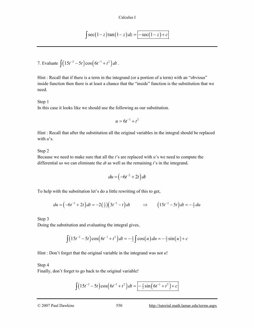
Calculus I
© 2007 Paul Dawkins 550 http://tutorial.math.lamar.edu/terms.aspx
( ) ( ) ( )sec 1 tan 1 sec 1z z dz z c− − = − − +∫
7. Evaluate ( ) ( )2 1 215 5 cos 6t t t t dt− −− +∫ .
Hint : Recall that if there is a term in the integrand (or a portion of a term) with an “obvious” inside function then there is at least a chance that the “inside” function is the substitution that we need. Step 1 In this case it looks like we should use the following as our substitution. 1 26u t t−= + Hint : Recall that after the substitution all the original variables in the integral should be replaced with u’s. Step 2 Because we need to make sure that all the t’s are replaced with u’s we need to compute the differential so we can eliminate the dt as well as the remaining t’s in the integrand.
( )26 2du t t dt−= − +
To help with the substitution let’s do a little rewriting of this to get,
( ) ( )( ) ( )2 2 25 55 26 2 2 3 15 5du t t dt t t dt t t dt du− − −= − + = − − ⇒ − = −
Step 3 Doing the substitution and evaluating the integral gives,
( ) ( ) ( ) ( )2 1 2 5 52 215 5 cos 6 cos sint t t t dt u du u c− −− + = − = − +∫ ∫
Hint : Don’t forget that the original variable in the integrand was not u! Step 4 Finally, don’t forget to go back to the original variable!
( ) ( ) ( )2 1 2 1 25215 5 cos 6 sin 6t t t t dt t t c− − −− + = − + +∫

Calculus I
© 2007 Paul Dawkins 551 http://tutorial.math.lamar.edu/terms.aspx
8. Evaluate ( ) 4 23 77 2 y yy y dy−−∫ e .
Hint : Recall that if there is a term in the integrand (or a portion of a term) with an “obvious” inside function then there is at least a chance that the “inside” function is the substitution that we need. Step 1 In this case it looks like we should use the following as our substitution.
4 27u y y= − Hint : Recall that after the substitution all the original variables in the integral should be replaced with u’s. Step 2 Because we need to make sure that all the y’s are replaced with u’s we need to compute the differential so we can eliminate the dy as well as the remaining y’s in the integrand.
( )34 14du y y dy= −
To help with the substitution let’s do a little rewriting of this to get,
( ) ( ) ( )3 3 3 124 14 2 7 2 7 2du y y dy y y dy y y dy du= − = − − ⇒ − = −
Step 3 Doing the substitution and evaluating the integral gives,
( ) 4 23 7 1 12 27 2 y y u uy y dy du c−− = − = − +∫ ∫e e e
Hint : Don’t forget that the original variable in the integrand was not u! Step 4 Finally, don’t forget to go back to the original variable!
( ) 4 2 4 23 7 7127 2 y y y yy y dy c− −− = − +∫ e e
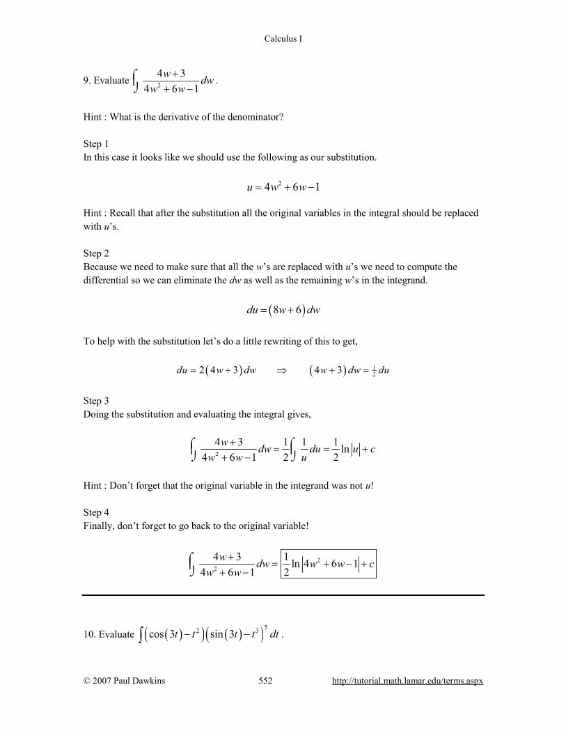
Calculus I
© 2007 Paul Dawkins 552 http://tutorial.math.lamar.edu/terms.aspx
9. Evaluate 2
4 34 6 1
w dww w
++ −
⌠⌡
.
Hint : What is the derivative of the denominator? Step 1 In this case it looks like we should use the following as our substitution. 24 6 1u w w= + − Hint : Recall that after the substitution all the original variables in the integral should be replaced with u’s. Step 2 Because we need to make sure that all the w’s are replaced with u’s we need to compute the differential so we can eliminate the dw as well as the remaining w’s in the integrand.
( )8 6du w dw= +
To help with the substitution let’s do a little rewriting of this to get,
( ) ( ) 122 4 3 4 3du w dw w dw du= + ⇒ + =
Step 3 Doing the substitution and evaluating the integral gives,
2
4 3 1 1 1 ln4 6 1 2 2
w dw du u cw w u
+= = +
+ −⌠ ⌠ ⌡ ⌡
Hint : Don’t forget that the original variable in the integrand was not u! Step 4 Finally, don’t forget to go back to the original variable!
22
4 3 1 ln 4 6 14 6 1 2
w dw w w cw w
+= + − +
+ −⌠⌡
10. Evaluate ( )( ) ( )( )52 3cos 3 sin 3t t t t dt− −∫ .

Calculus I
© 2007 Paul Dawkins 553 http://tutorial.math.lamar.edu/terms.aspx
Hint : Recall that if there is a term in the integrand (or a portion of a term) with an “obvious” inside function then there is at least a chance that the “inside” function is the substitution that we need. Step 1 In this case it looks like we should use the following as our substitution. ( ) 3sin 3u t t= − Hint : Recall that after the substitution all the original variables in the integral should be replaced with u’s. Step 2 Because we need to make sure that all the t’s are replaced with u’s we need to compute the differential so we can eliminate the dt as well as the remaining t’s in the integrand.
( )( )23cos 3 3du t t dt= −
To help with the substitution let’s do a little rewriting of this to get,
( )( ) ( )( )2 2 133 cos 3 cos 3du t t dt t t dt du= − ⇒ − =
Step 3 Doing the substitution and evaluating the integral gives,
( )( ) ( )( )52 3 5 61 13 18cos 3 sin 3t t t t dt u du u c− − = = +∫ ∫
Hint : Don’t forget that the original variable in the integrand was not u! Step 4 Finally, don’t forget to go back to the original variable!
( )( ) ( )( ) ( )( )5 62 3 3118cos 3 sin 3 sin 3t t t t dt t t c− − = − +∫
11. Evaluate ( )14 cos lnz z z dzz
− − − +
⌠⌡
e e .

Calculus I
© 2007 Paul Dawkins 554 http://tutorial.math.lamar.edu/terms.aspx
Hint : Recall that if there is a term in the integrand (or a portion of a term) with an “obvious” inside function then there is at least a chance that the “inside” function is the substitution that we need. Step 1 In this case it looks like we should use the following as our substitution. lnzu z−= +e Hint : Recall that after the substitution all the original variables in the integral should be replaced with u’s. Step 2 Because we need to make sure that all the z’s are replaced with u’s we need to compute the differential so we can eliminate the dz as well as the remaining z’s in the integrand.
( )1z
zdu dt−= − +e
Recall that, in most cases, we will also need to do a little manipulation of the differential prior to doing the substitution. In this case we don’t need to do that. Step 3 Doing the substitution and evaluating the integral gives,
( ) ( ) ( )14 cos ln 4cos 4sinz z z dz u du u cz
− − − + = = +
⌠⌡ ∫e e
Hint : Don’t forget that the original variable in the integrand was not u! Step 4 Finally, don’t forget to go back to the original variable!
( ) ( )14 cos ln 4sin lnz z zz dz z cz
− − − − + = + +
⌠⌡
e e e
12. Evaluate ( ) ( )12 tansec vv dv+∫ e .
Hint : Recall that if there is a term in the integrand (or a portion of a term) with an “obvious” inside function then there is at least a chance that the “inside” function is the substitution that we need.

Calculus I
© 2007 Paul Dawkins 555 http://tutorial.math.lamar.edu/terms.aspx
Step 1 In this case it looks like we should use the following as our substitution. ( )1 tanu v= + Hint : Recall that after the substitution all the original variables in the integral should be replaced with u’s. Step 2 Because we need to make sure that all the v’s are replaced with u’s we need to compute the differential so we can eliminate the dv as well as the remaining v’s in the integrand.
( )2secdu v dv=
Recall that, in most cases, we will also need to do a little manipulation of the differential prior to doing the substitution. In this case we don’t need to do that. Step 3 Doing the substitution and evaluating the integral gives,
( ) ( )12 tansec v u uv dv du c+ = = +∫ ∫e e e
Hint : Don’t forget that the original variable in the integrand was not u! Step 4 Finally, don’t forget to go back to the original variable!
( ) ( ) ( )1 12 tan tansec v vv dv c+ += +∫ e e
13. Evaluate ( ) ( ) ( )210sin 2 cos 2 cos 2 5x x x dx−∫ .
Hint : Recall that if there is a term in the integrand (or a portion of a term) with an “obvious” inside function then there is at least a chance that the “inside” function is the substitution that we need. Step 1 In this case it looks like we should use the following as our substitution.
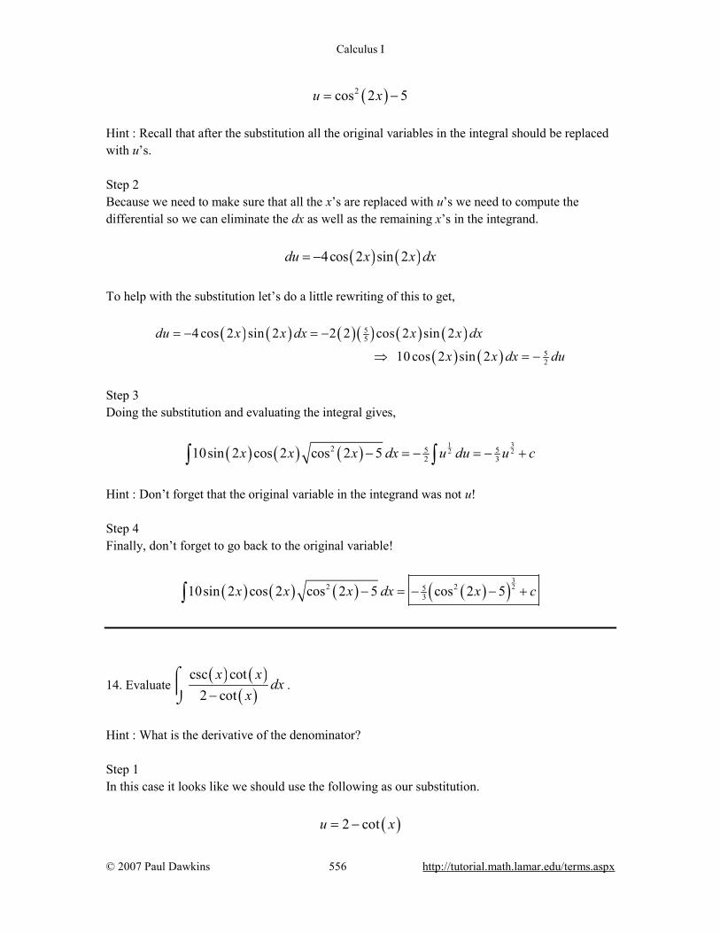
Calculus I
© 2007 Paul Dawkins 556 http://tutorial.math.lamar.edu/terms.aspx
( )2cos 2 5u x= − Hint : Recall that after the substitution all the original variables in the integral should be replaced with u’s. Step 2 Because we need to make sure that all the x’s are replaced with u’s we need to compute the differential so we can eliminate the dx as well as the remaining x’s in the integrand.
( ) ( )4cos 2 sin 2du x x dx= −
To help with the substitution let’s do a little rewriting of this to get,
( ) ( ) ( )( ) ( ) ( )( ) ( )
55
52
4 cos 2 sin 2 2 2 cos 2 sin 2
10 cos 2 sin 2
du x x dx x x dx
x x dx du
= − = −
⇒ = −
Step 3 Doing the substitution and evaluating the integral gives,
( ) ( ) ( )31
2 22 5 52 310sin 2 cos 2 cos 2 5x x x dx u du u c− = − = − +∫ ∫
Hint : Don’t forget that the original variable in the integrand was not u! Step 4 Finally, don’t forget to go back to the original variable!
( ) ( ) ( ) ( )( )322 25
310sin 2 cos 2 cos 2 5 cos 2 5x x x dx x c− = − − +∫
14. Evaluate ( ) ( )
( )csc cot
2 cotx x
dxx−
⌠⌡
.
Hint : What is the derivative of the denominator? Step 1 In this case it looks like we should use the following as our substitution. ( )2 cotu x= −
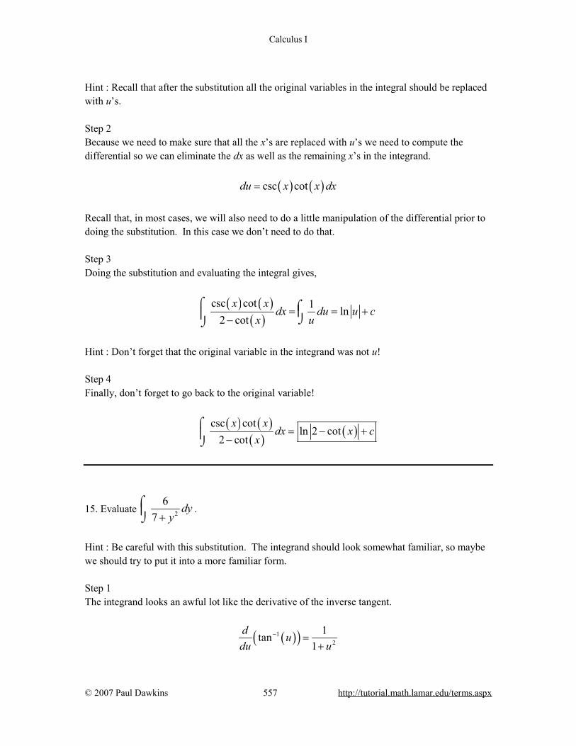
Calculus I
© 2007 Paul Dawkins 557 http://tutorial.math.lamar.edu/terms.aspx
Hint : Recall that after the substitution all the original variables in the integral should be replaced with u’s. Step 2 Because we need to make sure that all the x’s are replaced with u’s we need to compute the differential so we can eliminate the dx as well as the remaining x’s in the integrand.
( ) ( )csc cotdu x x dx=
Recall that, in most cases, we will also need to do a little manipulation of the differential prior to doing the substitution. In this case we don’t need to do that. Step 3 Doing the substitution and evaluating the integral gives,
( ) ( )( )
csc cot 1 ln2 cot
x xdx du u c
x u= = +
−⌠ ⌠ ⌡⌡
Hint : Don’t forget that the original variable in the integrand was not u! Step 4 Finally, don’t forget to go back to the original variable!
( ) ( )( ) ( )csc cot
ln 2 cot2 cot
x xdx x c
x= − +
−⌠⌡
15. Evaluate 2
67
dyy+
⌠⌡
.
Hint : Be careful with this substitution. The integrand should look somewhat familiar, so maybe we should try to put it into a more familiar form. Step 1 The integrand looks an awful lot like the derivative of the inverse tangent.
( )( )12
1tan1
d udu u
− =+
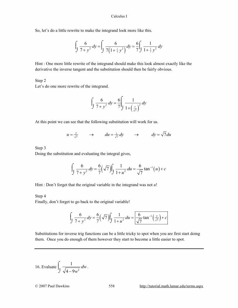
Calculus I
© 2007 Paul Dawkins 558 http://tutorial.math.lamar.edu/terms.aspx
So, let’s do a little rewrite to make the integrand look more like this.
( )2 22 1177
6 6 6 17 7 17 1
dy dy dyy yy
= =+ ++
⌠ ⌠⌠ ⌡ ⌡⌡
Hint : One more little rewrite of the integrand should make this look almost exactly like the derivative the inverse tangent and the substitution should then be fairly obvious. Step 2 Let’s do one more rewrite of the integrand.
( )22
7
6 6 17 7 1 y
dy dyy
=+ +
⌠⌠ ⌡ ⌡
At this point we can see that the following substitution will work for us.
17 7
7yu du dy dy du= → = → =
Step 3 Doing the substitution and evaluating the integral gives,
( ) ( )12 2
6 6 1 67 tan7 7 1 7
dy du u cy u
−= = ++ +
⌠ ⌠ ⌡⌡
Hint : Don’t forget that the original variable in the integrand was not u! Step 4 Finally, don’t forget to go back to the original variable!
( ) ( )12 2 7
6 6 1 67 tan7 7 1 7
ydy du cy u
−= = ++ +
⌠ ⌠ ⌡⌡ Substitutions for inverse trig functions can be a little tricky to spot when you are first start doing them. Once you do enough of them however they start to become a little easier to spot.
16. Evaluate 2
14 9
dww−
⌠⌡
.

Calculus I
© 2007 Paul Dawkins 559 http://tutorial.math.lamar.edu/terms.aspx
Hint : Be careful with this substitution. The integrand should look somewhat familiar, so maybe we should try to put it into a more familiar form. Step 1 The integrand looks an awful lot like the derivative of the inverse sine.
( )( )1
2
1sin1
d udu u
− =−
So, let’s do a little rewrite to make the integrand look more like this.
( )2 22 9944
1 1 1 124 9 14 1
dw dw dww ww
= =− −−
⌠ ⌠⌠ ⌡ ⌡⌡
Hint : One more little rewrite of the integrand should make this look almost exactly like the derivative the inverse sine and the substitution should then be fairly obvious. Step 2 Let’s do one more rewrite of the integrand.
( )2 232
1 1 124 9 1 w
dw dww
=− −
⌠⌠
⌡ ⌡
At this point we can see that the following substitution will work for us.
3 3 22 2 3wu du dw dw du= → = → =
Step 3 Doing the substitution and evaluating the integral gives,
( )1
2 2
1 1 2 1 1 sin2 3 34 9 1
dw du u cw u
− = = + − −
⌠ ⌠ ⌡ ⌡
Hint : Don’t forget that the original variable in the integrand was not u! Step 4 Finally, don’t forget to go back to the original variable!
( )1 322
1 1 sin34 9
wdw cw
−= +−
⌠⌡

Calculus I
© 2007 Paul Dawkins 560 http://tutorial.math.lamar.edu/terms.aspx
Substitutions for inverse trig functions can be a little tricky to spot when you are first start doing them. Once you do enough of them however they start to become a little easier to spot. 17. Evaluate each of the following integrals.
(a) 2
31 9
x dxx+
⌠⌡
(b) ( )42
3
1 9
x dxx+
⌠⌡
(c) 2
31 9
dxx+
⌠⌡
Hint : Make sure you pay attention to each of these and note the differences between each integrand and how that will affect the substitution and/or answer.
(a) 2
31 9
x dxx+
⌠⌡
Solution In this case it looks like the substitution should be
21 9u x= + Here is the differential for this substitution.
1618 3du x dx x dx du= ⇒ =
The integral is then,
22
3 1 1 1 1ln ln 1 91 9 6 6 6
x dx du u c x cx u
= = + = + ++
⌠ ⌠ ⌡ ⌡
(b) ( )42
3
1 9
x dxx+
⌠⌡
Solution The substitution and differential work for this part are identical to the previous part.
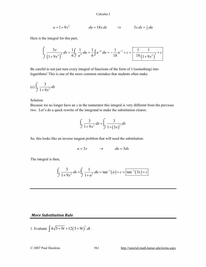
Calculus I
© 2007 Paul Dawkins 561 http://tutorial.math.lamar.edu/terms.aspx
2 161 9 18 3u x du x dx x dx du= + = ⇒ =
Here is the integral for this part,
( ) ( )4 3
4 342 2
3 1 1 1 1 1 16 6 18 181 9 1 9
x dx du u du u c cux x
− −= = = − + = − ++ +
⌠ ⌠ ⌡⌡∫
Be careful to not just turn every integral of functions of the form of 1/(something) into logarithms! This is one of the more common mistakes that students often make.
(c) 2
31 9
dxx+
⌠⌡
Solution Because we no longer have an x in the numerator this integral is very different from the previous two. Let’s do a quick rewrite of the integrand to make the substitution clearer.
( )22
3 31 9 1 3
dx dxx x
=+ +
⌠⌠ ⌡ ⌡
So, this looks like an inverse tangent problem that will need the substitution.
3 3u x du dx= → =
The integral is then,
( ) ( )1 12 2
3 1 tan tan 31 9 1
dx du u c x cx u
− −= = + = ++ +
⌠ ⌠ ⌡ ⌡
More Substitution Rule
1. Evaluate ( )74 5 9 12 5 9t t dt+ + +∫ .
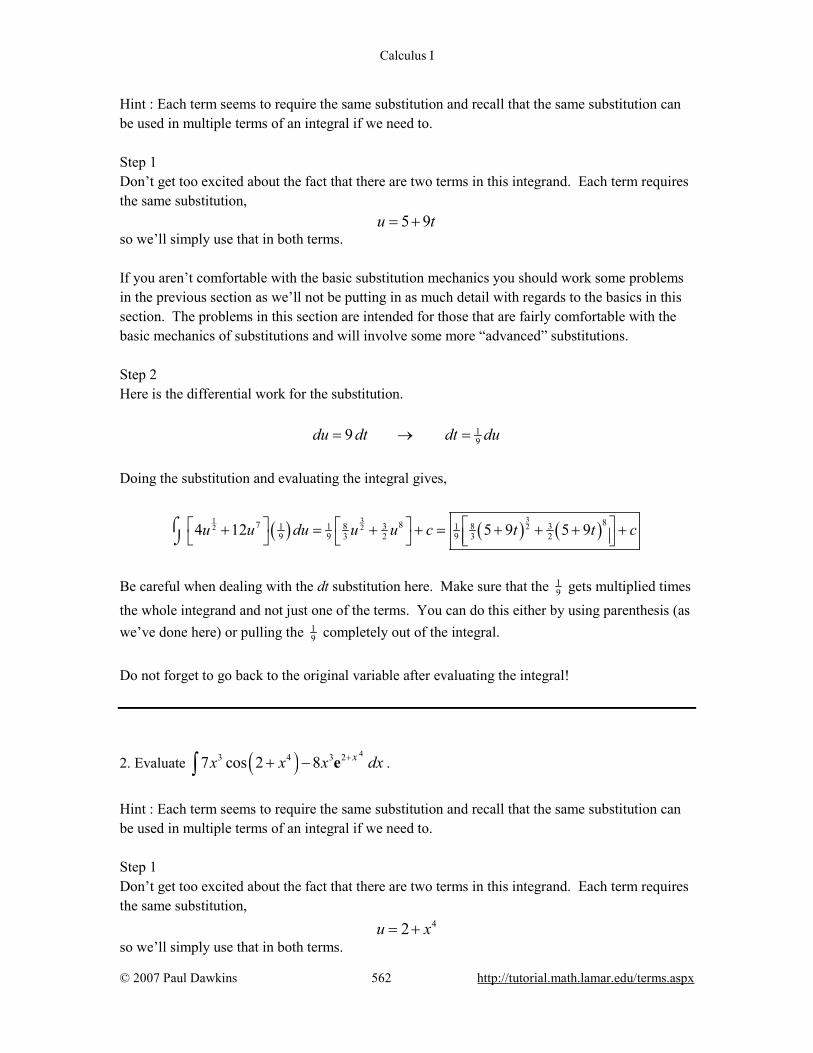
Calculus I
© 2007 Paul Dawkins 562 http://tutorial.math.lamar.edu/terms.aspx
Hint : Each term seems to require the same substitution and recall that the same substitution can be used in multiple terms of an integral if we need to. Step 1 Don’t get too excited about the fact that there are two terms in this integrand. Each term requires the same substitution, 5 9u t= + so we’ll simply use that in both terms. If you aren’t comfortable with the basic substitution mechanics you should work some problems in the previous section as we’ll not be putting in as much detail with regards to the basics in this section. The problems in this section are intended for those that are fairly comfortable with the basic mechanics of substitutions and will involve some more “advanced” substitutions. Step 2 Here is the differential work for the substitution.
199du dt dt du= → =
Doing the substitution and evaluating the integral gives,
( ) ( ) ( )33122 2 87 88 3 8 31 1 1
9 9 3 2 9 3 24 12 5 9 5 9u u du u u c t t c + = + + = + + + + ⌠⌡
Be careful when dealing with the dt substitution here. Make sure that the 1
9 gets multiplied times the whole integrand and not just one of the terms. You can do this either by using parenthesis (as we’ve done here) or pulling the 1
9 completely out of the integral. Do not forget to go back to the original variable after evaluating the integral!
2. Evaluate ( ) 43 4 3 27 cos 2 8 xx x x dx++ −∫ e .
Hint : Each term seems to require the same substitution and recall that the same substitution can be used in multiple terms of an integral if we need to. Step 1 Don’t get too excited about the fact that there are two terms in this integrand. Each term requires the same substitution, 42u x= + so we’ll simply use that in both terms.

Calculus I
© 2007 Paul Dawkins 563 http://tutorial.math.lamar.edu/terms.aspx
If you aren’t comfortable with the basic substitution mechanics you should work some problems in the previous section as we’ll not be putting in as much detail with regards to the basics in this section. The problems in this section are intended for those that are fairly comfortable with the basic mechanics of substitutions and will involve some more “advanced” substitutions. Step 2 Here is the differential work for the substitution.
3 3 144du x dx x dx du= → =
Before doing the actual substitution it might be convenient to factor an 3x out of the integrand as follows.
( ) ( )4 43 4 3 2 4 2 37 cos 2 8 7cos 2 8x xx x x dx x x dx+ + + − = + − ∫ ∫e e
Doing this should make the differential part (i.e. the du part) of the substitution clearer. Now, doing the substitution and evaluating the integral gives,
( ) ( )
( ) ( )
4
4
3 4 3 2 14
4 21 14 4
7 cos 2 8 7 cos 8
7sin 8 7sin 2 8
x u
u x
x x x dx u du
u c x c
+
+
+ − = −
= − + = + − +
∫ ∫e e
e e
Be careful when dealing with the dx substitution here. Make sure that the 1
4 gets multiplied times the whole integrand and not just one of the terms. You can do this either by using parenthesis around the whole integrand or pulling the 1
4 completely out of the integral (as we’ve done here). Do not forget to go back to the original variable after evaluating the integral!
3. Evaluate ( )
7 7
3 77
6 141 81 8
w w
wwdw+
−−
⌠⌡
e eee
.
Hint : Each term seems to require the same substitution and recall that the same substitution can be used in multiple terms of an integral if we need to. Step 1

Calculus I
© 2007 Paul Dawkins 564 http://tutorial.math.lamar.edu/terms.aspx
Don’t get too excited about the fact that there are two terms in this integrand. Each term requires the same substitution, 71 8 wu = − e so we’ll simply use that in both terms. If you aren’t comfortable with the basic substitution mechanics you should work some problems in the previous section as we’ll not be putting in as much detail with regards to the basics in this section. The problems in this section are intended for those that are fairly comfortable with the basic mechanics of substitutions and will involve some more “advanced” substitutions. Step 2 Here is the differential work for the substitution.
7 7 15656 w wdu dw dw du= − → = −e e
Before doing the actual substitution it might be convenient to factor an 7we out of the integrand as follows.
( ) ( )
7 77
3 37 77 7
6 14 6 141 8 1 81 8 1 8
w ww
w ww wdw dw
+ = + − −− −
⌠⌠ ⌡ ⌡
e e ee ee e
Doing this should make the differential part (i.e. the du part) of the substitution clearer. Now, doing the substitution and evaluating the integral gives,
( )( )
( )( )
7 73 21 1
56 563 77
27 7156
6 14 146 3 14ln1 81 8
3 1 8 14ln 1 8
w w
ww
w w
dw u du u u cu
c
− −
−
+ = − + = − − + +−−
= − − − + − +
⌠ ⌠ ⌡⌡
e eee
e e
Be careful when dealing with the dw substitution here. Make sure that the 1
56− gets multiplied times the whole integrand and not just one of the terms. You can do this either by using parenthesis around the whole integrand or pulling the 1
56− completely out of the integral (as we’ve done here). Do not forget to go back to the original variable after evaluating the integral!

Calculus I
© 2007 Paul Dawkins 565 http://tutorial.math.lamar.edu/terms.aspx
4. Evaluate ( )4 5 67 cos 2 3x x x dx− +∫ .
Hint : Recall that terms that do not need substitutions should not be in the integral when the substitution is being done. At this point we should know how to “break” integrals up so that we can get the terms that require a substitution into a one integral and those that don’t into another integral. Step 1 Clearly the first term does not need a substitution while the second term does need a substitution. So, we’ll first need to split up the integral as follows.
( ) ( )4 5 6 4 5 67 cos 2 3 7 cos 2 3x x x dx x dx x x dx− + = − +∫ ∫ ∫ Step 2 The substitution needed for the second integral is then, 62 3u x= + If you aren’t comfortable with the basic substitution mechanics you should work some problems in the previous section as we’ll not be putting in as much detail with regards to the basics in this section. The problems in this section are intended for those that are fairly comfortable with the basic mechanics of substitutions and will involve some more “advanced” substitutions. Step 3 Here is the differential work for the substitution.
5 5 11212du x dx x dx du= → =
Now, doing the substitution and evaluating the integrals gives,
( ) ( ) ( )
( )
4 5 6 4 57 7112 5 12
5 6715 12
7 cos 2 3 cos sin
sin 2 3
x x x dx x dx u du x u c
x x c
− + = − = − +
= − + +
∫ ∫ ∫
Do not forget to go back to the original variable after evaluating the integral!
5. Evaluate ( )
( )4sin 8
1 9cos 8z z
dzz
++
⌠⌡
e .
Calculus I
© 2007 Paul Dawkins 566 http://tutorial.math.lamar.edu/terms.aspx
Hint : Recall that terms that do not need substitutions should not be in the integral when the substitution is being done. At this point we should know how to “break” integrals up so that we can get the terms that require a substitution into a one integral and those that don’t into another integral. Step 1 Clearly the first term does not need a substitution while the second term does need a substitution. So, we’ll first need to split up the integral as follows.
( )( )
( )( )
4sin 8 4sin 81 9cos 8 1 9cos 8
z zz zdz dz dz
z z+ = +
+ +⌠ ⌠ ⌡ ⌡
∫e e
Step 2 The substitution needed for the second integral is then, ( )1 9cos 8u z= + If you aren’t comfortable with the basic substitution mechanics you should work some problems in the previous section as we’ll not be putting in as much detail with regards to the basics in this section. The problems in this section are intended for those that are fairly comfortable with the basic mechanics of substitutions and will involve some more “advanced” substitutions. Step 3 Here is the differential work for the substitution.
( ) ( ) 17272sin 8 sin 8du z dz z dz du= − → = −
Now, doing the substitution and evaluating the integrals gives,
( )( ) ( )1
18
4sin 8 4 1 ln 1 9cos 81 9cos 8 72
z z zzdz dz du z c
z u+ = − = − + +
+⌠ ⌠ ⌡⌡
∫e e e
Do not forget to go back to the original variable after evaluating the integral!
6. Evaluate 2 8 2 8 3 320 1 7 6w w w w dw− −+ + −∫ e e .
Hint : Recall that terms that do not need substitutions should not be in the integral when the substitution is being done. At this point we should know how to “break” integrals up so that we can get the terms that require a substitution into a one integral and those that don’t into another integral.

Calculus I
© 2007 Paul Dawkins 567 http://tutorial.math.lamar.edu/terms.aspx
Step 1 Clearly the first term needs a substitution while the second and third terms don’t. So, we’ll first need to split up the integral as follows.
2 8 2 8 3 2 8 2 8 33 320 1 7 6 20 1 7 6w w w ww w dw dw w w dw− − − −+ + − = + + −∫ ∫ ∫e e e e Step 2 The substitution needed for the first integral is then, 2 81 wu −= + e If you aren’t comfortable with the basic substitution mechanics you should work some problems in the previous section as we’ll not be putting in as much detail with regards to the basics in this section. The problems in this section are intended for those that are fairly comfortable with the basic mechanics of substitutions and will involve some more “advanced” substitutions. Step 3 Here is the differential work for the substitution.
2 8 2 8 188 w wdu dw dw du− −= − → = −e e
Now, doing the substitutions and evaluating the integrals gives,
( )
1132
3 432
3 42 3
2 8 2 8 3 33 208
45 7 93 4 2
2 8 45 7 93 4 2
20 1 7 6 7 6
1
w w
w
w w dw u du w w dw
u w w c
w w c
− −
−
+ + − = − + −
= − + − +
= − + + − +
∫ ∫ ∫e e
e
Do not forget to go back to the original variable after evaluating the integral!
7. Evaluate ( )3 244 7 9 5 3t t t dt+ − +∫ .
Hint : You can only do one substitution per integral. At this point we should know how to “break” integrals up so that we can get the terms that require different substitutions into different integrals. Step 1

Calculus I
© 2007 Paul Dawkins 568 http://tutorial.math.lamar.edu/terms.aspx
Clearly each term needs a separate substitution. So, we’ll first need to split up the integral as follows.
( ) ( )3 32 24 44 7 9 5 3 4 7 9 5 3t t t dt t dt t t dt+ − + = + − +∫ ∫ ∫ Step 2 The substitutions needed for the each integral are then, 24 7 5 3u t v t= + = + If you aren’t comfortable with the basic substitution mechanics you should work some problems in the previous section as we’ll not be putting in as much detail with regards to the basics in this section. The problems in this section are intended for those that are fairly comfortable with the basic mechanics of substitutions and will involve some more “advanced” substitutions. Step 3 Here is the differential work for each substitution.
1 17 107 10du dt dt du dv t dt t dt dv= → = = → =
Now, doing the substitutions and evaluating the integrals gives,
( )
( ) ( )
514 4
54
3 2 3 44 9 181 17 10 28 25
4 218128 25
4 7 9 5 3
4 7 5 3
t dt t t dt u du v dv u v c
t t c
+ − + = − = − +
= + − + +
∫ ∫ ∫ ∫
Do not forget to go back to the original variable after evaluating the integral!
8. Evaluate 2
23 2
6 3csc9 8 2
x x x dxx x
− − − + ⌠⌡
.
Hint : You can only do one substitution per integral. At this point we should know how to “break” integrals up so that we can get the terms that require different substitutions into different integrals. Step 1 Clearly each term needs a separate substitution. So, we’ll first need to split up the integral as follows.
Calculus I
© 2007 Paul Dawkins 569 http://tutorial.math.lamar.edu/terms.aspx
2 2
2 23 2 3 2
6 3 6 3csc csc9 8 2 9 8 2
x x x x x xdx dx dxx x x x
− − − = − − + − + ⌠ ⌠⌠
⌡ ⌡⌡
Step 2 The substitutions needed for the each integral are then,
3 2 39 82xu x x v= − + =
If you aren’t comfortable with the basic substitution mechanics you should work some problems in the previous section as we’ll not be putting in as much detail with regards to the basics in this section. The problems in this section are intended for those that are fairly comfortable with the basic mechanics of substitutions and will involve some more “advanced” substitutions. Step 3 Here is the differential work for each substitution.
( ) ( ) ( )2 2 2 13
3 22 3
3 18 3 6 6du x x dx x x dx x x dx du
dv dx dx dv
= − = − − → − = −
= → =
Now, doing the substitutions and evaluating the integrals gives,
( ) ( )
( )
22 2
3 2
3 21 23 3
32
6 3 1 1 2 1 2csc csc ln cot9 8 2 3 3 3 3
ln 9 8 cot x
x x x dx du v dv u v cx x u
x x c
− − = − − = − + + − +
= − − + + +
⌠ ⌠ ⌡⌡ ∫
Do not forget to go back to the original variable after evaluating the integral!
9. Evaluate ( )( ) ( )327 3 2 4 3 sin 3 8y y y y dy+ + + +∫ .
Hint : You can only do one substitution per integral. At this point we should know how to “break” integrals up so that we can get the terms that require different substitutions into different integrals. Step 1 Clearly each term needs a separate substitution. So, we’ll first need to split up the integral as follows.

Calculus I
© 2007 Paul Dawkins 570 http://tutorial.math.lamar.edu/terms.aspx
( ) ( ) ( ) ( ) ( ) ( )3 32 27 3 2 4 3 sin 3 8 7 3 2 4 3 sin 3 8y y y y dy y y y dy y dy+ + + + = + + + +∫ ∫ ∫ Step 2 The substitutions needed for the each integral are then,
24 3 3 8u y y v y= + = + If you aren’t comfortable with the basic substitution mechanics you should work some problems in the previous section as we’ll not be putting in as much detail with regards to the basics in this section. The problems in this section are intended for those that are fairly comfortable with the basic mechanics of substitutions and will involve some more “advanced” substitutions. Step 3 Here is the differential work for each substitution.
( ) ( ) ( ) 12
18
4 6 2 3 2 3 28
du y dy y dy y dy dudv dy dy dv
= + = + → + =
= → =
Now, doing the substitutions and evaluating the integrals gives,
( )( ) ( ) ( ) ( )
( ) ( )
32 3 47 71 12 8 8 8
427 18 8
7 3 2 4 3 sin 3 8 sin cos
4 3 cos 3 8
y y y y dy u du v dv u v c
y y y c
+ + + + = + = − +
= + − + +
∫ ∫ ∫
Do not forget to go back to the original variable after evaluating the integral!
10. Evaluate ( ) ( ) ( )2 2sec 2 9 7 tan 2 tan 2t t t dt + − ∫ .
Hint : Don’t let this one fool you. This is simply an integral that requires you to use the same substitution more than once. Step 1 This integral can be a little daunting at first glance. To do it all we need to notice is that the derivative of ( )tan x is ( )2sec x and we can notice that there is a ( )2sec 2t times the remaining
portion of the integrand and that portion only contains constants and tangents. So, it looks like the substitution is then,
( )tan 2u t=

Calculus I
© 2007 Paul Dawkins 571 http://tutorial.math.lamar.edu/terms.aspx
If you aren’t comfortable with the basic substitution mechanics you should work some problems in the previous section as we’ll not be putting in as much detail with regards to the basics in this section. The problems in this section are intended for those that are fairly comfortable with the basic mechanics of substitutions and will involve some more “advanced” substitutions. Step 2 Here is the differential work for the substitution.
( ) ( )2 2 122sec 2 sec 2du t dt t dt du= → =
Now, doing the substitution and evaluating the integrals gives,
( ) ( ) ( ) ( )( ) ( ) ( )( )
2 2 2 2 371 1 12 2 2 3
2 371 12 2 3
sec 2 9 7 tan 2 tan 2 9 7 9
9 tan 2 tan 2 tan 2
t t t dt u u du u u u c
t t t c
+ − = + − = + − +
= + − +
∫ ∫
Do not forget to go back to the original variable after evaluating the integral!
11. Evaluate 2
84 9
w dww
−+
⌠⌡
.
Hint : With the integrand written as it is here this problem can’t be done. Step 1 As written we can’t do this problem. In order to do this integral we’ll need to rewrite the integral as follows.
2 2 2
8 84 9 4 9 4 9
w wdw dw dww w w
−= −
+ + +⌠ ⌠ ⌠ ⌡ ⌡ ⌡
Step 2 Now, the first integral looks like it might be an inverse tangent (although we’ll need to do a rewrite of that integral) and the second looks like it’s a logarithm (with a quick substitution). So, here is the rewrite on the first integral.
2 2 249
8 8 14 9 9 1 4 9
w wdw dw dww w w
−= −
+ + +⌠⌠ ⌠ ⌡ ⌡⌡
Step 3

Calculus I
© 2007 Paul Dawkins 572 http://tutorial.math.lamar.edu/terms.aspx
Now we’ll need a substitution for each integral. Here are the substitutions we’ll need for each integral.
( )2 2 22 43 9so 4 9u w u w v w= = = +
Step 4 Here is the differential work for the substitution.
32 13 2 88du dw dw du dv wdw wdw dv= → = = → =
Now, doing the substitutions and evaluating the integrals gives,
( )
( )
14 13 82 2
1 24 2 13 3 8
8 8 3 1 1 1 tan ln4 9 9 2 1 8
tan ln 4 9
w dw du dv v u cw v v
w w c
−
−
− = − = − + + +
= − + +
⌠ ⌠ ⌠ ⌡ ⌡ ⌡
Do not forget to go back to the original variable after evaluating the integral!
12. Evaluate 2
7 21 25
x dxx
+
−
⌠⌡
.
Hint : With the integrand written as it is here this problem can’t be done. Step 1 As written we can’t do this problem. In order to do this integral we’ll need to rewrite the integral as follows.
2 2 2
7 2 7 21 25 1 25 1 25
x xdx dx dxx x x
+= +
− − −
⌠ ⌠ ⌠ ⌡ ⌡ ⌡
Step 2 Now, the second integral looks like it might be an inverse sine (although we’ll need to do a rewrite of that integral) and the first looks like a simple substitution will work for us. So, here is the rewrite on the second integral.
( )2 2 2
7 2 7 121 25 1 25 1 5
x xdx dx dxx x x
+= +
− − −
⌠⌠ ⌠
⌡ ⌡ ⌡

Calculus I
© 2007 Paul Dawkins 573 http://tutorial.math.lamar.edu/terms.aspx
Step 3 Now we’ll need a substitution for each integral. Here are the substitutions we’ll need for each integral.
( )2 2 21 25 5 so 25u x v x v x= − = = Step 4 Here is the differential work for the substitution.
1 150 550 5du x dx x dx du dv dx dx dv= − → = − = → =
Now, doing the substitutions and evaluating the integrals gives,
( )
( ) ( )
1 12 2
12
1
2 2
2 17 225 5
7 2 7 2 1 7 2 sin50 5 25 51 25 1
1 25 sin 5
x dx u du dv u v cx v
x x c
− −
−
+= − + = − + +
− −
= − − + +
⌠ ⌠ ⌡ ⌡∫
Do not forget to go back to the original variable after evaluating the integral!
13. Evaluate ( )87 48 3z z dz+∫ .
Hint : Use the “obvious” substitution and don’t forget that the substitution can be used more than once and in different ways. Step 1 Okay, the “obvious” substitution here is probably, 4 3 3 1
128 3 12u z du z dz z dz du= + → = → =
however, that doesn’t look like it might work because of the 7z . Step 2 Let’s do a quick rewrite of the integrand.
( ) ( ) ( )8 8 87 4 4 3 4 4 4 38 3 8 3 8 3z z dz z z z dz z z z dz+ = + = +∫ ∫ ∫ Step 3

Calculus I
© 2007 Paul Dawkins 574 http://tutorial.math.lamar.edu/terms.aspx
Now, notice that we can convert all of the z’s in the integrand except apparently for the 4z that is in the front. However, notice from the substitution that we can solve for 4z to get, ( )4 1
3 8z u= − Step 4 With this we can now do the substitution and evaluate the integral.
( ) ( ) ( )
( ) ( )( )
87 4 8 9 8 10 981 1 1 1 112 3 36 36 10 9
10 94 481 136 10 9
8 3 8 8
8 3 8 3
z z dz u u du u u du u u c
z z c
+ = − = − = − +
= + − + +
∫ ∫ ∫
Do not forget to go back to the original variable after evaluating the integral!
Area Problem 1. Estimate the area of the region between ( ) 3 22 4f x x x= − + the x-axis on [ ]1,4 using 6n =
and using, (a) the right end points of the subintervals for the height of the rectangles, (b) the left end points of the subintervals for the height of the rectangles and, (c) the midpoints of the subintervals for the height of the rectangles. (a) the right end points of the subintervals for the height of the rectangles, The widths of each of the subintervals for this problem are,
4 1 16 2
x −∆ = =
We don’t need to actually graph the function to do this problem. It would probably help to have a number line showing subintervals however. Here is that number line.
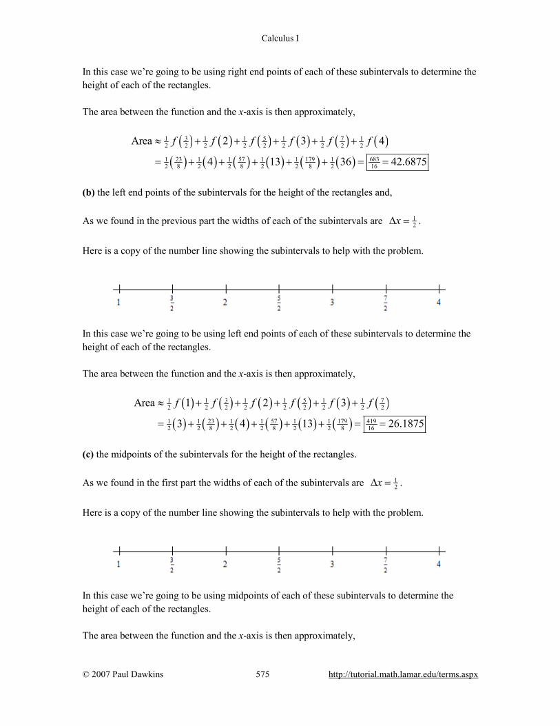
Calculus I
© 2007 Paul Dawkins 575 http://tutorial.math.lamar.edu/terms.aspx
In this case we’re going to be using right end points of each of these subintervals to determine the height of each of the rectangles. The area between the function and the x-axis is then approximately,
( ) ( ) ( ) ( ) ( ) ( )
( ) ( ) ( ) ( ) ( ) ( )
3 5 71 1 1 1 1 12 2 2 2 2 2 2 2 2
23 57 179 6831 1 1 1 1 12 8 2 2 8 2 2 8 2 16
Area 2 3 4
4 13 36 42.6875
f f f f f f≈ + + + + +
= + + + + + = =
(b) the left end points of the subintervals for the height of the rectangles and, As we found in the previous part the widths of each of the subintervals are 1
2x∆ = . Here is a copy of the number line showing the subintervals to help with the problem.
In this case we’re going to be using left end points of each of these subintervals to determine the height of each of the rectangles. The area between the function and the x-axis is then approximately,
( ) ( ) ( ) ( ) ( ) ( )
( ) ( ) ( ) ( ) ( ) ( )
3 5 71 1 1 1 1 12 2 2 2 2 2 2 2 2
23 57 179 4191 1 1 1 1 12 2 8 2 2 8 2 2 8 16
Area 1 2 3
3 4 13 26.1875
f f f f f f≈ + + + + +
= + + + + + = =
(c) the midpoints of the subintervals for the height of the rectangles. As we found in the first part the widths of each of the subintervals are 1
2x∆ = . Here is a copy of the number line showing the subintervals to help with the problem.
In this case we’re going to be using midpoints of each of these subintervals to determine the height of each of the rectangles. The area between the function and the x-axis is then approximately,

Calculus I
© 2007 Paul Dawkins 576 http://tutorial.math.lamar.edu/terms.aspx
( ) ( ) ( ) ( ) ( ) ( )
( ) ( ) ( ) ( ) ( ) ( )
5 7 9 13 151 1 1 1 11 1 12 4 2 4 2 4 2 4 2 4 2 4
181 207 337 619 1101 1831 10691 1 1 1 1 12 64 2 64 2 64 2 64 2 64 2 64 32
Area
33.40625
f f f f f f≈ + + + + +
= + + + + + = =
2. Estimate the area of the region between ( ) 24 2g x x= − + the x-axis on [ ]1,3− using
6n = and using, (a) the right end points of the subintervals for the height of the rectangles, (b) the left end points of the subintervals for the height of the rectangles and, (c) the midpoints of the subintervals for the height of the rectangles. (a) the right end points of the subintervals for the height of the rectangles, The widths of each of the subintervals for this problem are,
( )3 1 26 3
x− −
∆ = =
We don’t need to actually graph the function to do this problem. It would probably help to have a number line showing subintervals however. Here is that number line.
In this case we’re going to be using right end points of each of these subintervals to determine the height of each of the rectangles. The area between the function and the x-axis is then approximately,
( ) ( ) ( ) ( ) ( ) ( )
( ) ( ) ( ) ( ) ( ) ( )5 72 1 2 1 2 2 2 2
3 3 3 3 3 3 3 3 3 3
19 19 43 672 2 2 2 2 23 3 3 3 3 3 3 3 3 3
Area 1 3
4 4 4 3 4 4 4 11
7.420752
f f f f f f≈ − + + + + +
= − + − + − + − + − + −
=
(b) the left end points of the subintervals for the height of the rectangles and, As we found in the previous part the widths of each of the subintervals are 2
3x∆ = . Here is a copy of the number line showing the subintervals to help with the problem.

Calculus I
© 2007 Paul Dawkins 577 http://tutorial.math.lamar.edu/terms.aspx
In this case we’re going to be using left end points of each of these subintervals to determine the height of each of the rectangles. The area between the function and the x-axis is then approximately,
( ) ( ) ( ) ( ) ( ) ( )( ) ( ) ( ) ( ) ( ) ( )
5 72 2 1 2 1 2 2 23 3 3 3 3 3 3 3 3 3
19 19 43 672 2 2 2 2 23 3 3 3 3 3 3 3 3 3
Area 1 1
4 3 4 4 4 3 4 4
8.477135
f f f f f f≈ − + − + + + +
= − + − + − + − + − + −
=
(c) the midpoints of the subintervals for the height of the rectangles. As we found in the first part the widths of each of the subintervals are 2
3x∆ = . Here is a copy of the number line showing the subintervals to help with the problem.
In this case we’re going to be using midpoints of each of these subintervals to determine the height of each of the rectangles. The area between the function and the x-axis is then approximately,
( ) ( ) ( ) ( ) ( ) ( )( ) ( ) ( ) ( ) ( ) ( )
82 2 2 2 2 2 4 2 23 3 3 3 3 3 3 3 3 3
34 8222 222 2 2 2 2 23 3 3 3 3 3 3 3 3 3
Area 0 2
4 4 2 4 4 4 6 4
8.031494
f f f f f f≈ − + + + + +
= − + − + − + − + − + −
=
3. Estimate the area of the region between ( ) ( )3cos xh x x= − the x-axis on [ ]0,3 using 6n =
and using, (a) the right end points of the subintervals for the height of the rectangles, (b) the left end points of the subintervals for the height of the rectangles and, (c) the midpoints of the subintervals for the height of the rectangles.
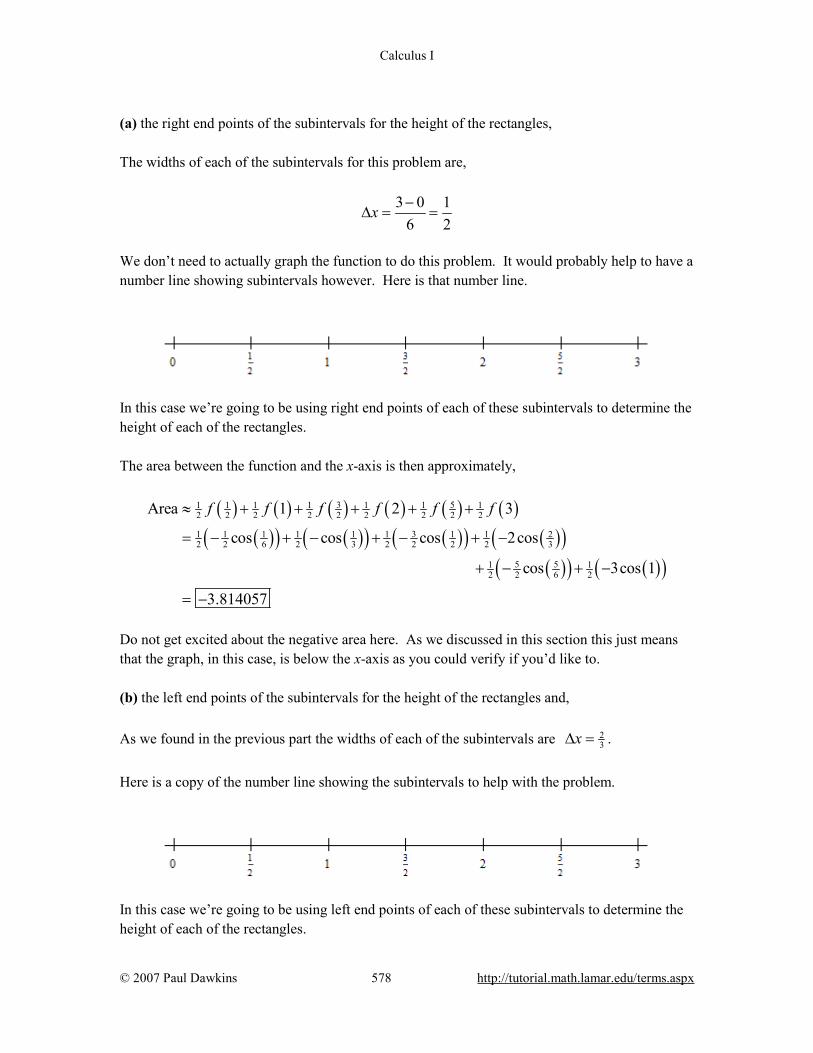
Calculus I
© 2007 Paul Dawkins 578 http://tutorial.math.lamar.edu/terms.aspx
(a) the right end points of the subintervals for the height of the rectangles, The widths of each of the subintervals for this problem are,
3 0 16 2
x −∆ = =
We don’t need to actually graph the function to do this problem. It would probably help to have a number line showing subintervals however. Here is that number line.
In this case we’re going to be using right end points of each of these subintervals to determine the height of each of the rectangles. The area between the function and the x-axis is then approximately,
( ) ( ) ( ) ( ) ( ) ( )( )( ) ( )( ) ( )( ) ( )( )
( )( ) ( )( )
3 51 1 1 1 1 1 12 2 2 2 2 2 2 2 2
31 1 1 1 1 1 1 1 22 2 6 2 3 2 2 2 2 3
5 51 12 2 6 2
Area 1 2 3
cos cos cos 2cos
cos 3cos 1
3.814057
f f f f f f≈ + + + + +
= − + − + − + −
+ − + −
= − Do not get excited about the negative area here. As we discussed in this section this just means that the graph, in this case, is below the x-axis as you could verify if you’d like to. (b) the left end points of the subintervals for the height of the rectangles and, As we found in the previous part the widths of each of the subintervals are 2
3x∆ = . Here is a copy of the number line showing the subintervals to help with the problem.
In this case we’re going to be using left end points of each of these subintervals to determine the height of each of the rectangles.
Calculus I
© 2007 Paul Dawkins 579 http://tutorial.math.lamar.edu/terms.aspx
The area between the function and the x-axis is then approximately,
( ) ( ) ( ) ( ) ( ) ( )( ) ( )( ) ( )( ) ( )( ) ( )( )
( )( )
3 51 1 1 1 1 1 12 2 2 2 2 2 2 2 2
31 1 1 1 1 1 1 1 1 22 2 2 6 2 3 2 2 2 2 3
5 512 2 6
Area 0 1 2
0 cos cos cos 2cos
cos
3.003604
f f f f f f≈ + + + + +
= + + − + − + − + −
+ −
= − Do not get excited about the negative area here. As we discussed in this section this just means that the graph, in this case, is below the x-axis as you could verify if you’d like to. (c) the midpoints of the subintervals for the height of the rectangles. As we found in the first part the widths of each of the subintervals are 2
3x∆ = . Here is a copy of the number line showing the subintervals to help with the problem.
In this case we’re going to be using midpoints of each of these subintervals to determine the height of each of the rectangles. The area between the function and the x-axis is then approximately,
( ) ( ) ( ) ( ) ( ) ( )( )( ) ( )( ) ( )( ) ( )( )
( )( ) ( )( )
3 5 7 91 1 1 1 1 1 1 112 4 2 4 2 4 2 4 2 4 2 4
3 5 5 7 71 1 1 1 1 1 12 4 12 2 4 4 2 4 12 2 4 12
9 31 1 11 112 4 4 2 4 12
Area
cos cos cos cos
cos cos
3.449532
f f f f f f≈ + + + + +
= − + − + − + −
+ − + −
= − Do not get excited about the negative area here. As we discussed in this section this just means that the graph, in this case, is below the x-axis as you could verify if you’d like to. 4. Estimate the net area between ( ) 2 58 12f x x x= − − and the x-axis on [ ]2,2− using 8n =
and the midpoints of the subintervals for the height of the rectangles. Without looking at a graph of the function on the interval does it appear that more of the area is above or below the x-axis?
Calculus I
© 2007 Paul Dawkins 580 http://tutorial.math.lamar.edu/terms.aspx
Step 1 First let’s estimate the area between the function and the x-axis on the interval. The widths of each of the subintervals for this problem are,
( )2 2 18 2
x− −
∆ = =
We don’t need to actually graph the function to do this problem. It would probably help to have a number line showing subintervals however. Here is that number line.
Now, we’ll be using midpoints of each of these subintervals to determine the height of each of the rectangles. The area between the function and the x-axis is then approximately,
( ) ( ) ( ) ( ) ( ) ( ) ( ) ( )7 5 3 3 5 71 1 1 1 1 1 1 1 1 12 4 2 4 2 4 2 4 2 4 2 4 2 4 2 4Area 6f f f f f f f f≈ − + − + − + − + + + + = −
We’ll leave it to you to check all the function evaluations. They get a little messy, but after all the arithmetic is done we get a net area of -6. Step 2 Now, as we (hopefully) recall from the discussion in this section area above the x-axis is positive and area below the x-axis is negative. In this case we have estimated that the net area is -6 and so, assuming that our estimate is accurate, it looks like we should have more area is below the x-axis as above it. Graph For reference purposes here is the graph of the function with the area shaded in and as we can see it does appear that there is slightly more area below as above the x-axis.
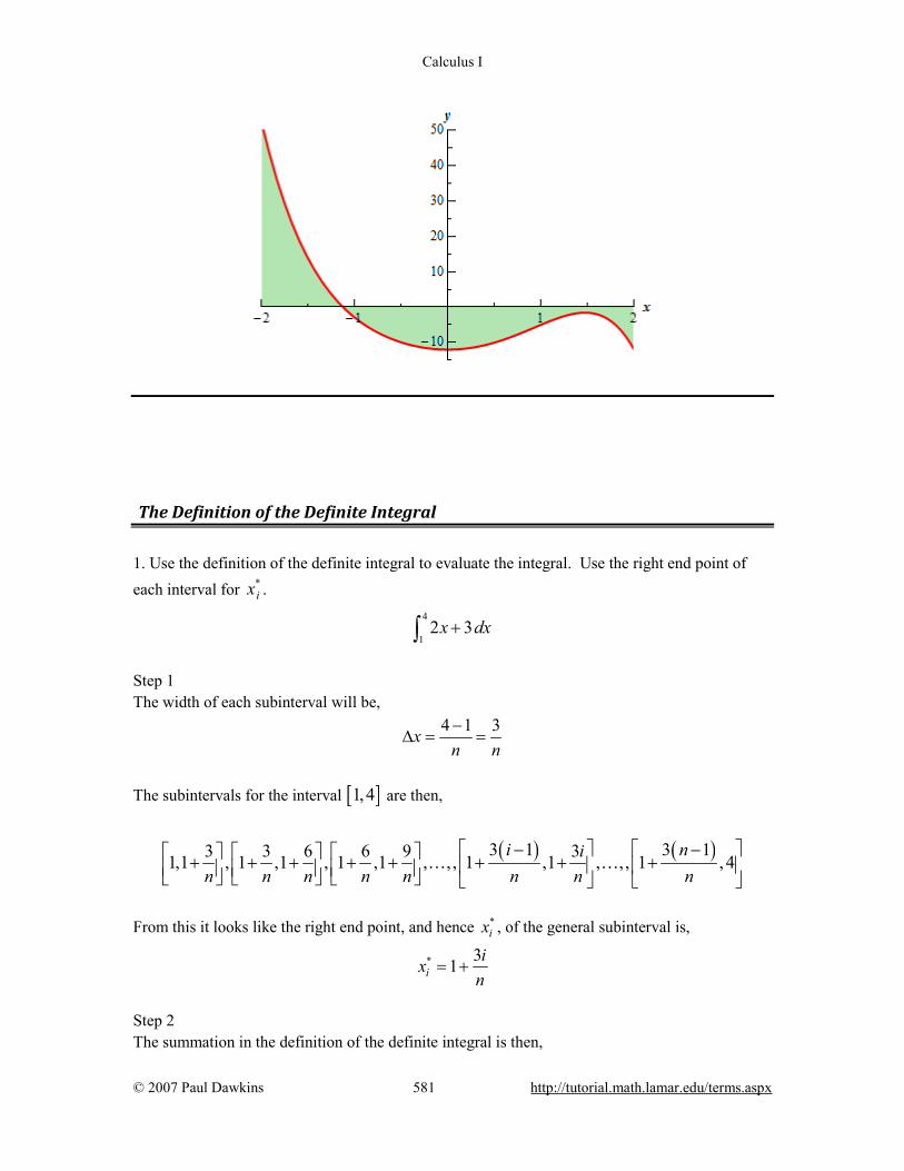
Calculus I
© 2007 Paul Dawkins 581 http://tutorial.math.lamar.edu/terms.aspx
The Definition of the Definite Integral 1. Use the definition of the definite integral to evaluate the integral. Use the right end point of each interval for *
ix . 4
12 3x dx+∫
Step 1 The width of each subinterval will be,
4 1 3xn n−
∆ = =
The subintervals for the interval [ ]1,4 are then,
( ) ( )3 1 3 13 3 6 6 9 31,1 , 1 ,1 , 1 ,1 , , , 1 ,1 , , , 1 , 4i ni
n n n n n n n n− − + + + + + + + +
… …
From this it looks like the right end point, and hence *
ix , of the general subinterval is,
* 31iix
n= +
Step 2 The summation in the definition of the definite integral is then,
Calculus I
© 2007 Paul Dawkins 582 http://tutorial.math.lamar.edu/terms.aspx
( )*2
1 1 1
3 3 15 182 1 3n n n
ii i i
i if x xn n n n= = =
∆ = + + = + ∑ ∑ ∑
Step 3 Now we need to use the formulas from the Summation Notation section in the Extras chapter to “evaluate” the summation.
( )
( ) ( )
*2 2
1 1 1 1 1
2
15 18 1 1815
11 18 9 915 152
n n n n n
ii i i i i
if x x in n n n
n n nnn n n
= = = = =
∆ = + = +
+ += + = +
∑ ∑ ∑ ∑ ∑
Step 4 Finally, we can use the definition of the definite integral to determine the value of the integral.
( )4 *
11
9 9 92 3 lim lim 15 lim 24 24n
in n ni
nx dx f x xn n→∞ →∞ →∞
=
+ + = ∆ = + = + = ∑∫
2. Use the definition of the definite integral to evaluate the integral. Use the right end point of each interval for *
ix .
( )1
06 1x x dx−∫
Step 1 The width of each subinterval will be,
1 0 1xn n−
∆ = =
The subintervals for the interval [ ]1,4 are then,
1 1 2 2 3 1 10, , , , , , , , , , , , ,1i i nn n n n n n n n
− −
… …
From this it looks like the right end point, and hence *
ix , of the general subinterval is,
*i
ixn
=
Step 2
Calculus I
© 2007 Paul Dawkins 583 http://tutorial.math.lamar.edu/terms.aspx
The summation in the definition of the definite integral is then,
( )2
*3 2
1 1 1
6 1 6 61n n n
ii i i
i i i if x xn n n n n= = =
∆ = − = − ∑ ∑ ∑
Step 3 Now we need to use the formulas from the Summation Notation section in the Extras chapter to “evaluate” the summation.
( )
( ) ( ) ( )
2* 2
3 2 3 21 1 1 1 1
2
3 2 2
6 6 6 6
1 2 1 16 6 2 3 1 3 36 2
n n n n n
ii i i i i
i if x x i in n n n
n n n n n n n nn n n n
= = = = =
∆ = − = − + + + + + +
= − = −
∑ ∑ ∑ ∑ ∑
Step 4 Finally, we can use the definition of the definite integral to determine the value of the integral.
( ) ( )21 *
201
2 3 1 3 36 1 lim lim 2 3 1n
in ni
n n nx x dx f x xn n→∞ →∞
=
+ + +− = ∆ = − = − = −
∑∫
3. Evaluate : ( )4 3 2
44
cos1
x xdx
x+
+⌠⌡
e
Solution There really isn’t much to this problem other than use Property 2 from the notes on this section.
( )4 3 2
44
cos0
1
x xdx
x+
=+
⌠⌡
e
4. Determine the value of ( )6
119 f x dx∫ given that ( )
11
67f x dx = −∫ .
Solution There really isn’t much to this problem other than use the properties from the notes of this section until we get the given interval at which point we use the given value.

Calculus I
© 2007 Paul Dawkins 584 http://tutorial.math.lamar.edu/terms.aspx
( ) ( )
( )
( )
6 6
11 1111
6
9 9 Property 3
9 Property 1
9 7 63
f x dx f x dx
f x dx
=
= −
= − − =
∫ ∫∫
5. Determine the value of ( ) ( )11
66 10g x f x dx−∫ given that ( )
11
67f x dx = −∫ and
( )11
624g x dx =∫ .
Solution There really isn’t much to this problem other than use the properties from the notes of this section until we get the given intervals at which point we use the given values.
( ) ( ) ( ) ( )
( ) ( )
( ) ( )
11 11 11
6 6 6
11 11
6 6
6 10 6 10 Property 4
6 10 Property 3
6 24 10 7 214
g x f x dx g x dx f x dx
g x dx f x dx
− = −
= −
= − − =
∫ ∫ ∫∫ ∫
6. Determine the value of ( )9
2f x dx∫ given that ( )
2
53f x dx =∫ and ( )
9
58f x dx =∫ .
Step 1 First we need to use Property 5 from the notes of this section to break up the integral into two integrals that use the same limits as the integrals given in the problem statement. Note that we won’t worry about whether the limits are in correct place at this point.
( ) ( ) ( )9 5 9
2 2 5f x dx f x dx f x dx= +∫ ∫ ∫
Step 2 Finally, all we need to do is use Property 1 from the notes of this section to interchange the limits on the first integral so they match up with the limits on the given integral. We can then use the given values to determine the value of the integral.
Calculus I
© 2007 Paul Dawkins 585 http://tutorial.math.lamar.edu/terms.aspx
( ) ( ) ( ) ( )9 2 9
2 5 53 8 5f x dx f x dx f x dx= − + = − + =∫ ∫ ∫
7. Determine the value of ( )20
4f x dx
−∫ given that ( )0
42f x dx
−= −∫ , ( )
0
3119f x dx =∫ and
( )31
2021f x dx = −∫ .
Step 1 First we need to use Property 5 from the notes of this section to break up the integral into three integrals that use the same limits as the integrals given in the problem statement. Note that we won’t worry about whether the limits are in correct place at this point.
( ) ( ) ( ) ( )20 0 31 20
4 4 0 31f x dx f x dx f x dx f x dx
− −= + +∫ ∫ ∫ ∫
Step 2 Finally, all we need to do is use Property 1 from the notes of this section to interchange the limits on the second integral so they match up with the limits on the given integral. We can then use the given values to determine the value of the integral.
( ) ( ) ( ) ( ) ( ) ( )20 0 0 20
4 4 31 312 19 21 42f x dx f x dx f x dx f x dx
− −= − + = − − + − = −∫ ∫ ∫ ∫
8. For 4
13 2x dx−∫ sketch the graph of the integrand and use the area interpretation of the
definite integral to determine the value of the integral. Step 1 Here is the graph of the integrand, ( ) 3 2f x x= − , on the interval [ ]1,4 .
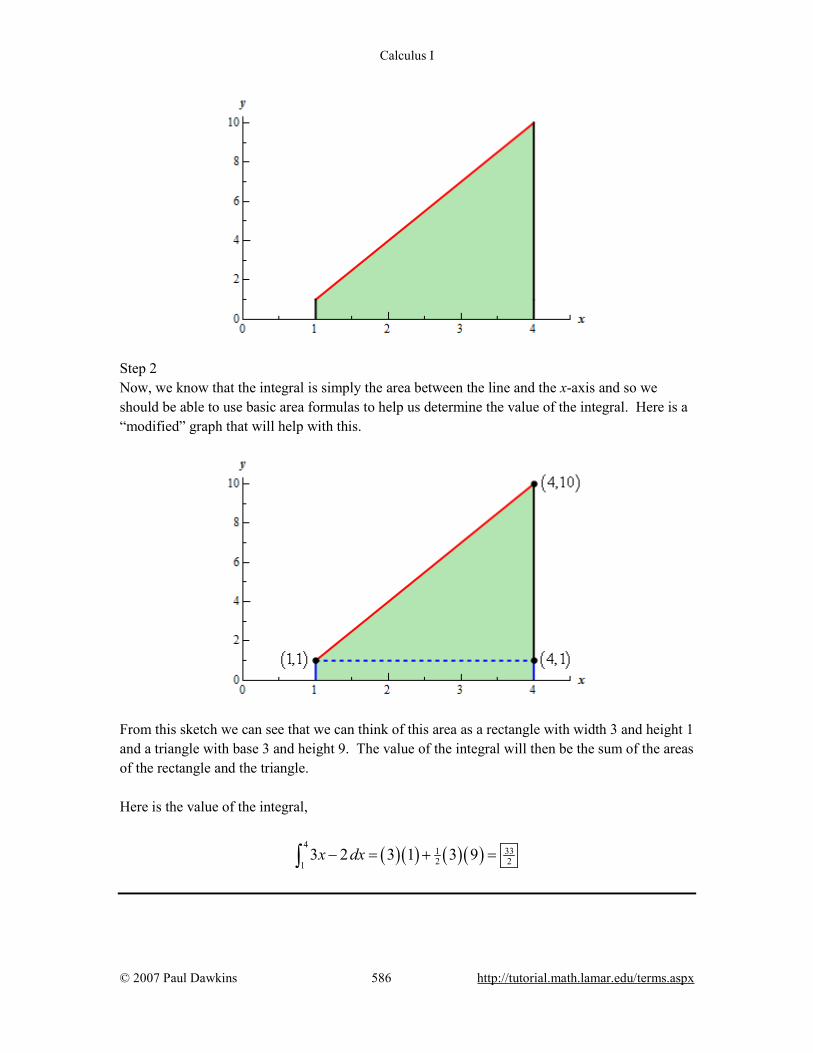
Calculus I
© 2007 Paul Dawkins 586 http://tutorial.math.lamar.edu/terms.aspx
Step 2 Now, we know that the integral is simply the area between the line and the x-axis and so we should be able to use basic area formulas to help us determine the value of the integral. Here is a “modified” graph that will help with this.
From this sketch we can see that we can think of this area as a rectangle with width 3 and height 1 and a triangle with base 3 and height 9. The value of the integral will then be the sum of the areas of the rectangle and the triangle. Here is the value of the integral,
( )( ) ( )( )4
3312 21
3 2 3 1 3 9x dx− = + =∫
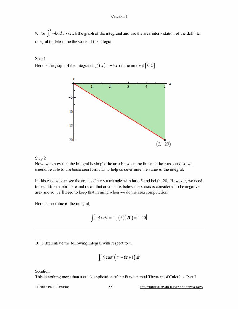
Calculus I
© 2007 Paul Dawkins 587 http://tutorial.math.lamar.edu/terms.aspx
9. For 5
04x dx−∫ sketch the graph of the integrand and use the area interpretation of the definite
integral to determine the value of the integral. Step 1 Here is the graph of the integrand, ( ) 4f x x= − on the interval [ ]0,5 .
Step 2 Now, we know that the integral is simply the area between the line and the x-axis and so we should be able to use basic area formulas to help us determine the value of the integral. In this case we can see the area is clearly a triangle with base 5 and height 20. However, we need to be a little careful here and recall that area that is below the x-axis is considered to be negative area and so we’ll need to keep that in mind when we do the area computation. Here is the value of the integral,
( )( )5
120
4 5 20 50x dx− = − = −∫ 10. Differentiate the following integral with respect to x.
( )2 2
49cos 6 1
xt t dt− +∫
Solution This is nothing more than a quick application of the Fundamental Theorem of Calculus, Part I.
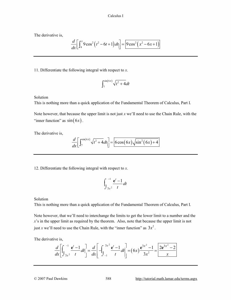
Calculus I
© 2007 Paul Dawkins 588 http://tutorial.math.lamar.edu/terms.aspx
The derivative is,
( ) ( )2 2 2 2
49cos 6 1 9cos 6 1
xd t t dt x xdx
− + = − + ∫
11. Differentiate the following integral with respect to x.
( )sin 6 2
74
xt dt+∫
Solution This is nothing more than a quick application of the Fundamental Theorem of Calculus, Part I. Note however, that because the upper limit is not just x we’ll need to use the Chain Rule, with the “inner function” as ( )sin 6x .
The derivative is,
( ) ( ) ( )
sin 6 2 2
74 6cos 6 sin 6 4
xd t dt x xdx
+ = + ∫
12. Differentiate the following integral with respect to x.
2
1
3
1t
xdt
t
− −⌠⌡
e
Solution This is nothing more than a quick application of the Fundamental Theorem of Calculus, Part I. Note however, that we’ll need to interchange the limits to get the lower limit to a number and the x’s in the upper limit as required by the theorem. Also, note that because the upper limit is not just x we’ll need to use the Chain Rule, with the “inner function” as 23x . The derivative is,
( )2 2 2
2
1
21
3 3 3
3
1 1 1 2 263
xt t
x
x xd ddt dt xdx t dx t x x
−
−
− − − −= − = =
⌠ ⌠ ⌡ ⌡
e e e e
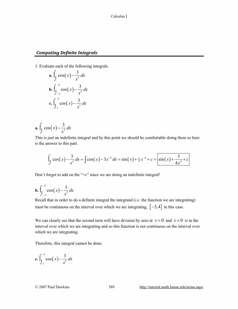
Calculus I
© 2007 Paul Dawkins 589 http://tutorial.math.lamar.edu/terms.aspx
Computing Definite Integrals 1. Evaluate each of the following integrals.
a. ( ) 5
3cos x dxx
−⌠⌡
b. ( )4
53
3cos x dxx−
−⌠⌡
c. ( )4
51
3cos x dxx
−⌠⌡
a. ( ) 5
3cos x dxx
−⌠⌡
This is just an indefinite integral and by this point we should be comfortable doing them so here is the answer to this part.
( ) ( ) ( ) ( )5 4345 4
3 3cos cos 3 sin sin4
x dx x x dx x x c x cx x
− −− = − = + + = + +⌠⌡ ∫
Don’t forget to add on the “+c” since we are doing an indefinite integral!
b. ( )4
53
3cos x dxx−
−⌠⌡
Recall that in order to do a definite integral the integrand (i.e. the function we are integrating) must be continuous on the interval over which we are integrating, [ ]3,4− in this case.
We can clearly see that the second term will have division by zero at 0x = and 0x = is in the interval over which we are integrating and so this function is not continuous on the interval over which we are integrating. Therefore, this integral cannot be done.
c. ( )4
51
3cos x dxx
−⌠⌡

Calculus I
© 2007 Paul Dawkins 590 http://tutorial.math.lamar.edu/terms.aspx
Now, the function still has a division by zero problem in the second term at 0x = . However,
unlike the previous part 0x = does not fall in the interval over which we are integrating, [ ]1,4 in
this case. This integral can therefore be done. Here is the work for this integral.
( ) ( ) ( )
( ) ( ) ( ) ( )
( ) ( ) ( ) ( )
44 4 55 411 1
4 4
3 3cos cos 3 sin4
3 3sin 4 sin 14 4 4 1
3 3 765sin 4 sin 1 sin 4 sin 11024 4 1024
x dx x x dx xx x
− − = − = +
= + − −
= + − − = − −
⌠⌡ ∫
2. Evaluate the following integral, if possible. If it is not possible clearly explain why it is not possible to evaluate the integral.
6 3 2
112 9 2x x dx− +∫
Step 1 First we need to integrate the function.
( ) 66 3 2 4 3
1 112 9 2 3 3 2x x dx x x x− + = − +∫
Recall that we don’t need to add the “+c” in the definite integral case as it will just cancel in the next step. Step 2 The final step is then just to do the evaluation. We’ll leave the basic arithmetic to you to verify and only show the results of the evaluation. Make sure that you evaluate the upper limit first and then subtract off the evaluation at the lower limit. Here is the answer for this problem.
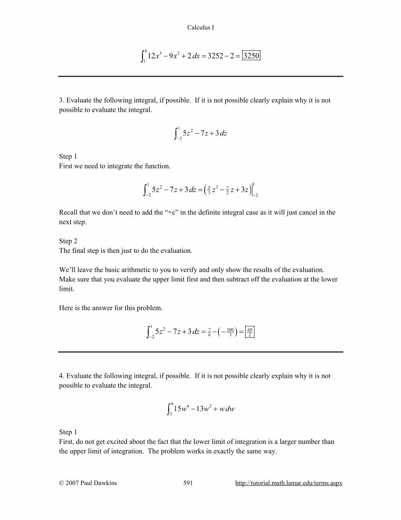
Calculus I
© 2007 Paul Dawkins 591 http://tutorial.math.lamar.edu/terms.aspx
6 3 2
112 9 2 3252 2 3250x x dx− + = − =∫
3. Evaluate the following integral, if possible. If it is not possible clearly explain why it is not possible to evaluate the integral.
1 2
25 7 3z z dz
−− +∫
Step 1 First we need to integrate the function.
( ) 11 2 35 73 22 2
5 7 3 3z z dz z z z− −
− + = − +∫ Recall that we don’t need to add the “+c” in the definite integral case as it will just cancel in the next step. Step 2 The final step is then just to do the evaluation. We’ll leave the basic arithmetic to you to verify and only show the results of the evaluation. Make sure that you evaluate the upper limit first and then subtract off the evaluation at the lower limit. Here is the answer for this problem.
( )1 2 7 100 69
6 3 225 7 3z z dz
−− + = − − =∫
4. Evaluate the following integral, if possible. If it is not possible clearly explain why it is not possible to evaluate the integral.
0 4 2
315 13w w w dw− +∫
Step 1 First, do not get excited about the fact that the lower limit of integration is a larger number than the upper limit of integration. The problem works in exactly the same way.
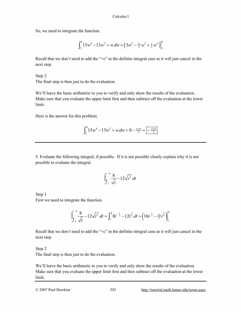
Calculus I
© 2007 Paul Dawkins 592 http://tutorial.math.lamar.edu/terms.aspx
So, we need to integrate the function.
( ) 00 4 2 5 2 213 13 23 3
15 13 3w w wdw w w w− + = − +∫ Recall that we don’t need to add the “+c” in the definite integral case as it will just cancel in the next step. Step 2 The final step is then just to do the evaluation. We’ll leave the basic arithmetic to you to verify and only show the results of the evaluation. Make sure that you evaluate the upper limit first and then subtract off the evaluation at the lower limit. Here is the answer for this problem.
0 4 2 1233 12332 23
15 13 0w w wdw− + = − = −∫
5. Evaluate the following integral, if possible. If it is not possible clearly explain why it is not possible to evaluate the integral.
43
1
8 12 t dtt
−⌠⌡
Step 1 First we need to integrate the function.
( )3 51 12 2 2 2
4 443 2451 11
8 12 8 12 16t dt t t dt t tt
−− = − = −⌠⌡ ∫
Recall that we don’t need to add the “+c” in the definite integral case as it will just cancel in the next step. Step 2 The final step is then just to do the evaluation. We’ll leave the basic arithmetic to you to verify and only show the results of the evaluation. Make sure that you evaluate the upper limit first and then subtract off the evaluation at the lower limit.
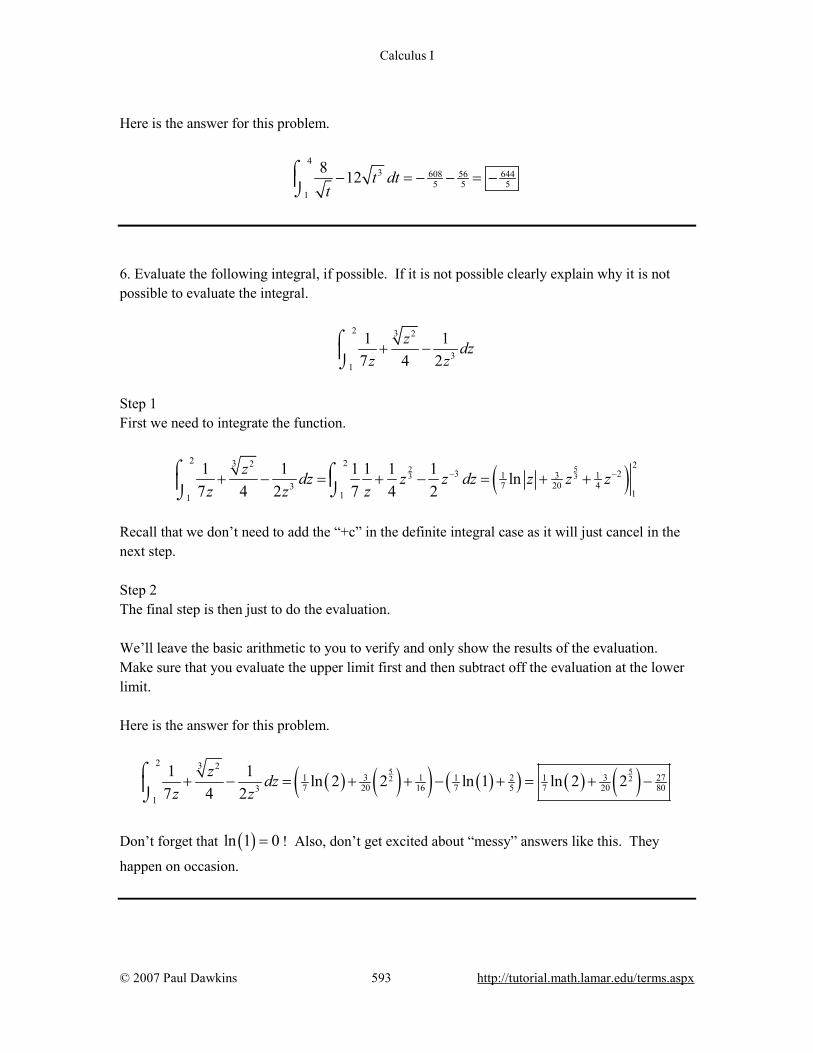
Calculus I
© 2007 Paul Dawkins 593 http://tutorial.math.lamar.edu/terms.aspx
Here is the answer for this problem.
43 608 56 644
5 5 51
8 12 t dtt
− = − − = −⌠⌡
6. Evaluate the following integral, if possible. If it is not possible clearly explain why it is not possible to evaluate the integral.
2 3 2
31
1 17 4 2
z dzz z
+ −⌠⌡
Step 1 First we need to integrate the function.
( )523 3
2 23 2 23 231 1
7 20 43111
1 1 1 1 1 1 ln7 4 2 7 4 2
z dz z z dz z z zz z z
− −+ − = + − = + +⌠ ⌠ ⌡⌡ Recall that we don’t need to add the “+c” in the definite integral case as it will just cancel in the next step. Step 2 The final step is then just to do the evaluation. We’ll leave the basic arithmetic to you to verify and only show the results of the evaluation. Make sure that you evaluate the upper limit first and then subtract off the evaluation at the lower limit. Here is the answer for this problem.
( ) ( )( ) ( )( ) ( ) ( )5 52 2
2 3 23 3 271 1 1 2 1
7 20 16 7 5 7 20 8031
1 1 ln 2 2 ln 1 ln 2 27 4 2
z dzz z
+ − = + + − + = + −⌠⌡
Don’t forget that ( )ln 1 0= ! Also, don’t get excited about “messy” answers like this. They
happen on occasion.
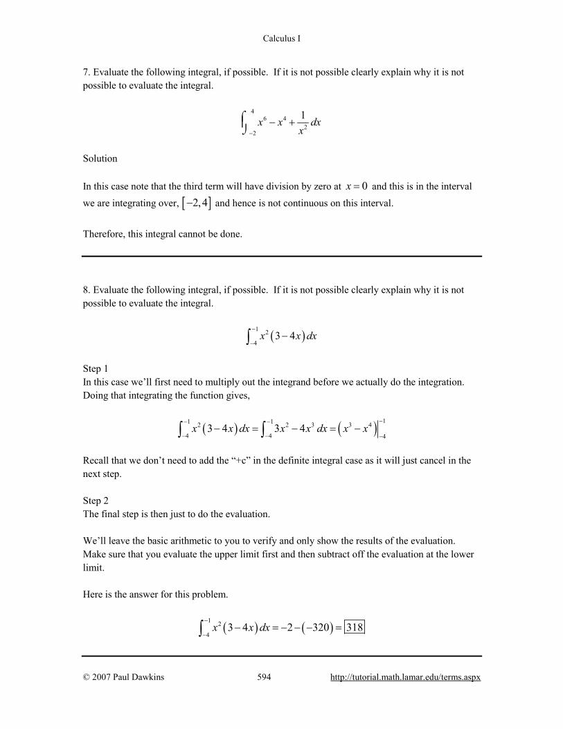
Calculus I
© 2007 Paul Dawkins 594 http://tutorial.math.lamar.edu/terms.aspx
7. Evaluate the following integral, if possible. If it is not possible clearly explain why it is not possible to evaluate the integral.
46 4
22
1x x dxx−
− +⌠⌡
Solution In this case note that the third term will have division by zero at 0x = and this is in the interval
we are integrating over, [ ]2,4− and hence is not continuous on this interval.
Therefore, this integral cannot be done. 8. Evaluate the following integral, if possible. If it is not possible clearly explain why it is not possible to evaluate the integral.
( )1 2
43 4x x dx
−
−−∫
Step 1 In this case we’ll first need to multiply out the integrand before we actually do the integration. Doing that integrating the function gives,
( ) ( ) 11 12 2 3 3 4
4 4 43 4 3 4x x dx x x dx x x
−− −
− − −− = − = −∫ ∫
Recall that we don’t need to add the “+c” in the definite integral case as it will just cancel in the next step. Step 2 The final step is then just to do the evaluation. We’ll leave the basic arithmetic to you to verify and only show the results of the evaluation. Make sure that you evaluate the upper limit first and then subtract off the evaluation at the lower limit. Here is the answer for this problem.
( ) ( )1 2
43 4 2 320 318x x dx
−
−− = − − − =∫
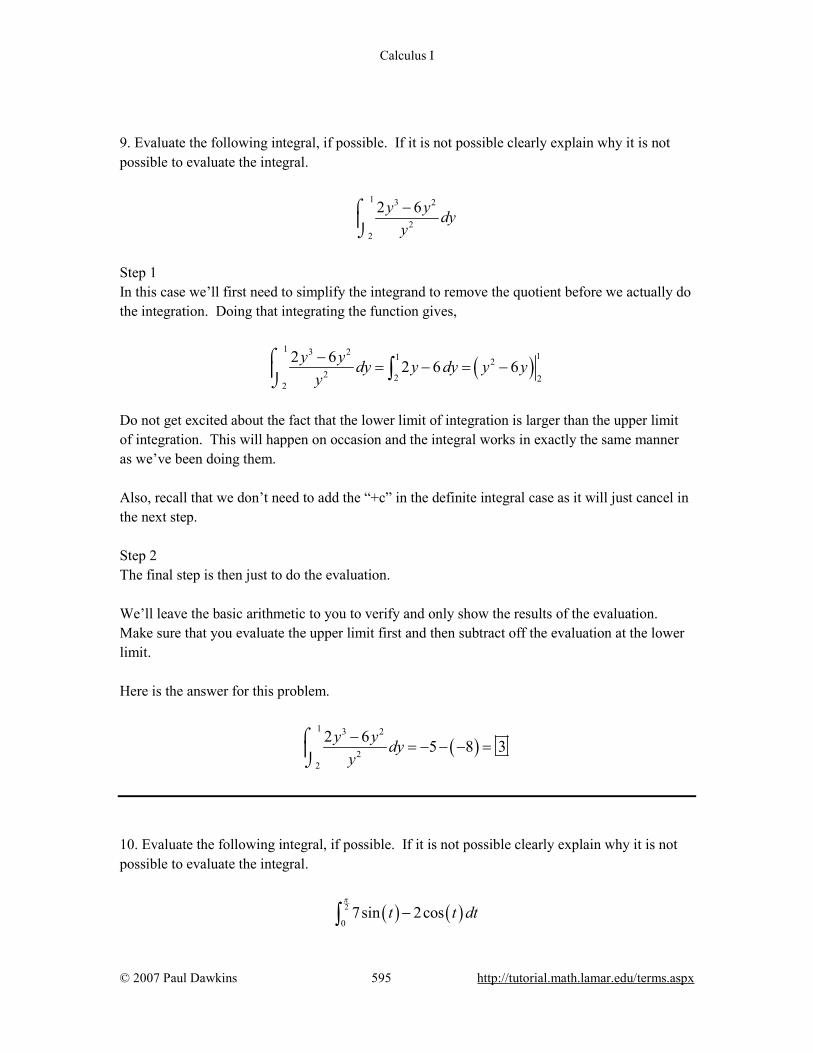
Calculus I
© 2007 Paul Dawkins 595 http://tutorial.math.lamar.edu/terms.aspx
9. Evaluate the following integral, if possible. If it is not possible clearly explain why it is not possible to evaluate the integral.
1 3 2
22
2 6y y dyy−⌠
⌡
Step 1 In this case we’ll first need to simplify the integrand to remove the quotient before we actually do the integration. Doing that integrating the function gives,
( )1 3 2 11 2
2 2 22
2 6 2 6 6y y dy y dy y yy−
= − = −⌠⌡ ∫
Do not get excited about the fact that the lower limit of integration is larger than the upper limit of integration. This will happen on occasion and the integral works in exactly the same manner as we’ve been doing them. Also, recall that we don’t need to add the “+c” in the definite integral case as it will just cancel in the next step. Step 2 The final step is then just to do the evaluation. We’ll leave the basic arithmetic to you to verify and only show the results of the evaluation. Make sure that you evaluate the upper limit first and then subtract off the evaluation at the lower limit. Here is the answer for this problem.
( )1 3 2
22
2 6 5 8 3y y dyy−
= − − − =⌠⌡
10. Evaluate the following integral, if possible. If it is not possible clearly explain why it is not possible to evaluate the integral.
( ) ( )2
07sin 2cost t dt
π
−∫

Calculus I
© 2007 Paul Dawkins 596 http://tutorial.math.lamar.edu/terms.aspx
Step 1 First we need to integrate the function.
( ) ( ) ( ) ( )( )2 2
007sin 2cos 7cos 2sint t dt t t
π π
− = − −∫ Recall that we don’t need to add the “+c” in the definite integral case as it will just cancel in the next step. Step 2 The final step is then just to do the evaluation. We’ll leave the basic arithmetic to you to verify and only show the results of the evaluation. Make sure that you evaluate the upper limit first and then subtract off the evaluation at the lower limit. Here is the answer for this problem.
( ) ( ) ( )2
07sin 2cos 2 7 5t t dt
π
− = − − − =∫
11. Evaluate the following integral, if possible. If it is not possible clearly explain why it is not possible to evaluate the integral.
( ) ( )0
sec tan 1z z dzπ
−∫
Solution Be careful with this integral. Recall that,
( ) ( ) ( ) ( )( )
sin1sec tancos cos
zz z
z z= =
Also recall that ( )2cos 0π = and that 2x π= is in the interval we are integrating over, [ ]0,π and
hence is not continuous on this interval. Therefore, this integral cannot be done.
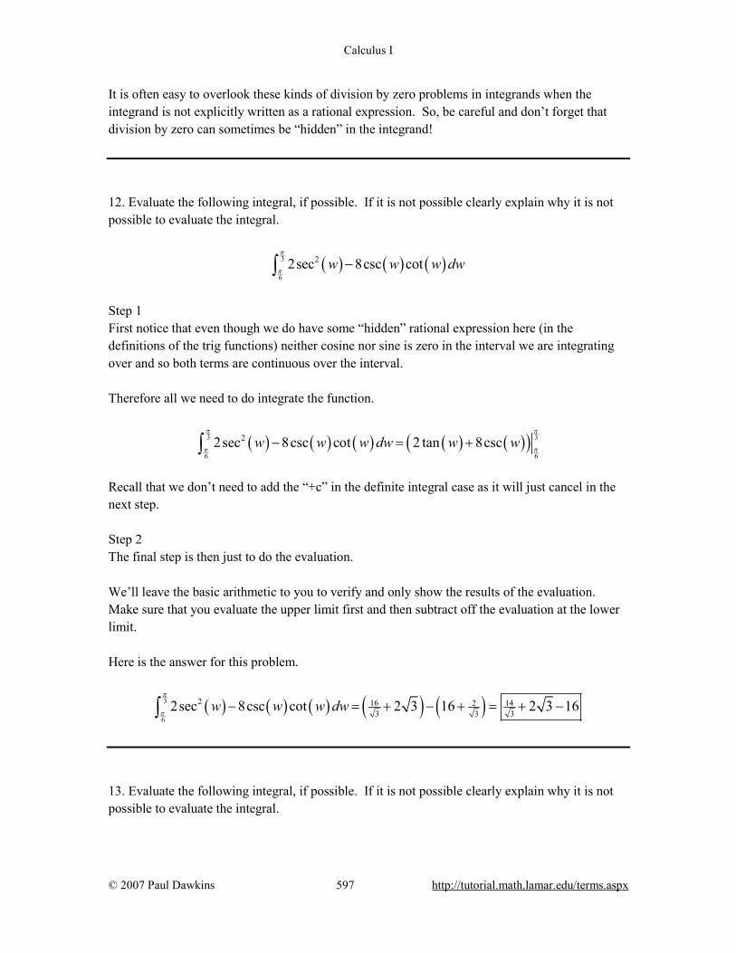
Calculus I
© 2007 Paul Dawkins 597 http://tutorial.math.lamar.edu/terms.aspx
It is often easy to overlook these kinds of division by zero problems in integrands when the integrand is not explicitly written as a rational expression. So, be careful and don’t forget that division by zero can sometimes be “hidden” in the integrand! 12. Evaluate the following integral, if possible. If it is not possible clearly explain why it is not possible to evaluate the integral.
( ) ( ) ( )3
6
22sec 8csc cotw w w dwπ
π−∫
Step 1 First notice that even though we do have some “hidden” rational expression here (in the definitions of the trig functions) neither cosine nor sine is zero in the interval we are integrating over and so both terms are continuous over the interval. Therefore all we need to do integrate the function.
( ) ( ) ( ) ( ) ( )( )3 3
66
22sec 8csc cot 2 tan 8cscw w w dw w wπ π
ππ− = +∫
Recall that we don’t need to add the “+c” in the definite integral case as it will just cancel in the next step. Step 2 The final step is then just to do the evaluation. We’ll leave the basic arithmetic to you to verify and only show the results of the evaluation. Make sure that you evaluate the upper limit first and then subtract off the evaluation at the lower limit. Here is the answer for this problem.
( ) ( ) ( ) ( ) ( )3
6
2 16 2 143 3 3
2sec 8csc cot 2 3 16 2 3 16w w w dwπ
π− = + − + = + −∫
13. Evaluate the following integral, if possible. If it is not possible clearly explain why it is not possible to evaluate the integral.
Calculus I
© 2007 Paul Dawkins 598 http://tutorial.math.lamar.edu/terms.aspx
2
20
11
x dxx
++
⌠⌡
e
Step 1 First we need to integrate the function.
( )( )2 21
2 00
1 tan1
x xdx xx
−+ = ++
⌠⌡
e e
Recall that we don’t need to add the “+c” in the definite integral case as it will just cancel in the next step. Step 2 The final step is then just to do the evaluation. We’ll leave the basic arithmetic to you to verify and only show the results of the evaluation. Make sure that you evaluate the upper limit first and then subtract off the evaluation at the lower limit. Here is the answer for this problem.
( )( ) ( )( ) ( )2
2 1 0 1 2 142
0
1 tan 2 tan 1 tan 2 11
x dxx
π− − −+ = + − + = + − −+
⌠⌡
e e e e
Note that ( )1
4tan 1 π− = but ( )1tan 2− doesn’t have a “nice” answer and so was left as is.
14. Evaluate the following integral, if possible. If it is not possible clearly explain why it is not possible to evaluate the integral.
2
5
27 y dyy
−
−
+⌠⌡
e
Step 1 First we need to integrate the function.
( )2
2
55
27 7 2lny ydy yy
−−
−−
+ = +⌠⌡
e e

Calculus I
© 2007 Paul Dawkins 599 http://tutorial.math.lamar.edu/terms.aspx
Recall that we don’t need to add the “+c” in the definite integral case as it will just cancel in the next step. Step 2 The final step is then just to do the evaluation. We’ll leave the basic arithmetic to you to verify and only show the results of the evaluation. Make sure that you evaluate the upper limit first and then subtract off the evaluation at the lower limit. Here is the answer for this problem.
( ) ( ) ( ) ( ) ( )( )2
2 5 2 5
5
27 7 2ln 2 7 2ln 5 7 2 ln 2 ln 5y dyy
−− − − −
−
+ = + − − + − = − + −⌠⌡
e e e e e
15. Evaluate the following integral, if possible. If it is not possible clearly explain why it is not possible to evaluate the integral.
( )4
0f t dt∫ where ( ) 2
2 11 3 1
t tf t
t t>
= − ≤
Hint : Recall that integrals we can always “break up” an integral as follows,
( ) ( ) ( )b c b
a a cf x dx f x dx f x dx= +∫ ∫ ∫
See if you can find a good choice for “c” that will make this integral doable. Step 1 This integral can’t be done as a single integral give the obvious change of the function at 1t = which is in the interval over which we are integrating. However, recall that we can always break up an integral at any point and 1t = seems to be a good point to do this. Breaking up the integral at 1t = gives,
( ) ( ) ( )4 1 4
0 0 1f t dt f t dt f t dt= +∫ ∫ ∫

Calculus I
© 2007 Paul Dawkins 600 http://tutorial.math.lamar.edu/terms.aspx
So, in the first integral we have 0 1t≤ ≤ and so we can use ( ) 21 3f t t= − in the first integral.
Likewise, in the second integral we have 1 4t≤ ≤ and so we can use ( ) 2f t t= in the second
integral. Making these function substitutions gives,
( )4 1 42
0 0 11 3 2f t dt t dt t dt= − +∫ ∫ ∫
Step 2 All we need to do at this point is evaluate each integral. Here is that work.
( ) ( ) [ ] [ ]14 1 4 42 3 2
10 0 1 01 3 2 0 0 16 1 15f t dt t dt t dt t t t= − + = − + = − + − =∫ ∫ ∫
16. Evaluate the following integral, if possible. If it is not possible clearly explain why it is not possible to evaluate the integral.
( )1
6g z dz
−∫ where ( ) 2 24 2z
z zg z
z− > −
= ≤ − e
Hint : Recall that integrals we can always “break up” an integral as follows,
( ) ( ) ( )b c b
a a cf x dx f x dx f x dx= +∫ ∫ ∫
See if you can find a good choice for “c” that will make this integral doable. Step 1 This integral can’t be done as a single integral give the obvious change of the function at 2z = − which is in the interval over which we are integrating. However, recall that we can always break up an integral at any point and 2z = − seems to be a good point to do this. Breaking up the integral at 2z = − gives,
( ) ( ) ( )1 2 1
6 6 2g z dz g z dz g z dz
−
− − −= +∫ ∫ ∫

Calculus I
© 2007 Paul Dawkins 601 http://tutorial.math.lamar.edu/terms.aspx
So, in the first integral we have 6 2z− ≤ ≤ − and so we can use ( ) 4 zg z = e in the first integral.
Likewise, in the second integral we have 2 1z− ≤ ≤ and so we can use ( ) 2g z z= − in the
second integral. Making these function substitutions gives,
( )1 2 1
6 6 24 2zg z dz dz z dz
−
− − −= + −∫ ∫ ∫e
Step 2 All we need to do at this point is evaluate each integral. Here is that work.
( ) ( ) ( )( )
2 11 2 1 2126 6 2 6 2
2 6 2 63 152 2
4 2 4 2
4 4 6 4 4
z zg z dz dz z dz z z−−
− − − − −
− − − −
= + − = + −
= − + − − = − +
∫ ∫ ∫e e
e e e e
17. Evaluate the following integral, if possible. If it is not possible clearly explain why it is not possible to evaluate the integral.
6
32 10x dx−∫
Hint : In order to do this integral we need to “remove” the absolute value bars from the integrand and we should know how to do that by this point. Step 1 We’ll need to “remove” the absolute value bars in order to do this integral. However, in order to do that we’ll need to know where 2 10x − is positive and negative. Since 2 10x − is the equation of a line is should be fairly clear that we have the following positive/negative nature of the function.
5 2 10 05 2 10 0
x xx x
< ⇒ − <> ⇒ − >
Step 2 So, to remove the absolute value bars all we need to do then is break the integral up at 5x = .
6 5 6
3 3 52 10 2 10 2 10x dx x dx x dx− = − + −∫ ∫ ∫

Calculus I
© 2007 Paul Dawkins 602 http://tutorial.math.lamar.edu/terms.aspx
So, in the first integral we have 3 5x≤ ≤ and so we have ( )2 10 2 10x x− = − − in the first
integral. Likewise, in the second integral we have 5 6x≤ ≤ and so we have 2 10 2 10x x− = −
in the second integral. Or,
( )6 5 6
3 3 52 10 2 10 2 10x dx x dx x dx− = − − + −∫ ∫ ∫
Step 3 All we need to do at this point is evaluate each integral. Here is that work.
( ) ( )[ ] ( )
5 66 5 6 2 2
3 3 5 3 52 10 2 10 2 10 10 10
25 21 24 25 5
x dx x dx x dx x x x x− = − + + − = − + + −
= − + − − − =
∫ ∫ ∫
18. Evaluate the following integral, if possible. If it is not possible clearly explain why it is not possible to evaluate the integral.
0
14 3w dw
−+∫
Hint : In order to do this integral we need to “remove” the absolute value bars from the integrand and we should know how to do that by this point. Step 1 We’ll need to “remove” the absolute value bars in order to do this integral. However, in order to do that we’ll need to know where 4 3w+ is positive and negative. Since 4 3w+ is the equation a line is should be fairly clear that we have the following positive/negative nature of the function.
3434
4 3 04 3 0
w ww w
< − ⇒ + <
> − ⇒ + >
Step 2 So, to remove the absolute value bars all we need to do then is break the integral up at 3
4w = − .
34
34
0 0
1 14 3 4 3 4 3w dw w dw w dw
−
− − −+ = + + +∫ ∫ ∫
Calculus I
© 2007 Paul Dawkins 603 http://tutorial.math.lamar.edu/terms.aspx
So, in the first integral we have 3
41 w− ≤ ≤ − and so we have ( )4 3 4 3w w+ = − + in the first
integral. Likewise, in the second integral we have 34 0w− ≤ ≤ and so we have
4 3 4 3w w+ = + in the second integral. Or,
( )34
34
0 0
1 14 3 4 3 4 3w dw w dw w dw
−
− − −+ = − + + +∫ ∫ ∫
Step 3 All we need to do at this point is evaluate each integral. Here is that work.
( ) ( )( )
3344
3 34 4
00 0 2 2
1 1 1
9 9 58 8 4
4 3 4 3 4 3 2 3 2 3
1 0
w dw w dw w dw w w w w−−
− − − − −+ = − − + + = − − + +
= − + − − =
∫ ∫ ∫
Substitution Rule for Definite Integrals 1. Evaluate the following integral, if possible. If it is not possible clearly explain why it is not possible to evaluate the integral.
( ) ( )1 64 2 5
03 4 10 2x x x x dx+ + −∫
Step 1 The first step that we need to do is do the substitution. At this point you should be fairly comfortable with substitutions. If you are not comfortable with substitutions you should go back to the substitution sections and work some problems there. The substitution for this problem is,
2 510 2u x x= + − Step 2 Here is the actual substitution work for this problem.
Calculus I
© 2007 Paul Dawkins 604 http://tutorial.math.lamar.edu/terms.aspx
( ) ( ) ( )4 4 4 1520 5 5 4 4
0 : 2 1: 9
du x x dx x x dx x x dx du
x u x u
= + = + → + =
= = − = =
As we did in the notes for this section we are also going to convert the limits to u’s to avoid having to deal with the back substitution after doing the integral. Here is the integral after the substitution.
( )( )1 964 2 5 6350 2
3 4 10 2x x x x dx u du−
+ + − =∫ ∫ Step 3 The integral is then,
( )( ) ( )( )1 6 94 2 5 7 14,349,2913 335 35 3520
3 4 10 2 4,782,969 128x x x x dx u−
+ + − = = − − =∫ Do not get excited about “messy” or “large” answers. They will happen on occasion so don’t worry about them when the happen. 2. Evaluate the following integral, if possible. If it is not possible clearly explain why it is not possible to evaluate the integral.
( )
( )
4
0
8cos 2
9 5sin 2
tdt
t
π
−
⌠⌡
Step 1 The first step that we need to do is do the substitution. At this point you should be fairly comfortable with substitutions. If you are not comfortable with substitutions you should go back to the substitution sections and work some problems there. The substitution for this problem is,
( )9 5sin 2u t= −
Step 2 Here is the actual substitution work for this problem.
Calculus I
© 2007 Paul Dawkins 605 http://tutorial.math.lamar.edu/terms.aspx
( ) ( ) 1
10
4
10cos 2 cos 20 : 9 : 4
du t dt t dt dut u t uπ
= − → = −
= = = =
As we did in the notes for this section we are also going to convert the limits to u’s to avoid having to deal with the back substitution after doing the integral. Here is the integral after the substitution.
( )
( )12
44
810 9
0
8cos 2
9 5sin 2
tdt u du
t
π
−= −−
⌠⌡
∫
Step 3 The integral is then,
( )( )
( )12
4 48 16 8245 5 5 59
0
8cos 2
9 5sin 2
tdt u
t
π
= − = − − − =−
⌠⌡
3. Evaluate the following integral, if possible. If it is not possible clearly explain why it is not possible to evaluate the integral.
( ) ( )0 3sin cosz z dz
π∫ Step 1 The first step that we need to do is do the substitution. At this point you should be fairly comfortable with substitutions. If you are not comfortable with substitutions you should go back to the substitution sections and work some problems there. The substitution for this problem is,
( )cosu z=
Step 2 Here is the actual substitution work for this problem.
( ) ( )sin sin
: 1 0 : 1du z dz z dz du
z u z uπ
= − → = −
= = − = =
Calculus I
© 2007 Paul Dawkins 606 http://tutorial.math.lamar.edu/terms.aspx
As we did in the notes for this section we are also going to convert the limits to u’s to avoid having to deal with the back substitution after doing the integral. Here is the integral after the substitution.
( ) ( )0 13 3
1sin cosz z dz u du
π −= −∫ ∫
Step 3 The integral is then,
( ) ( ) ( )0 13 41 1 1
4 4 41sin cos 0z z dz u
π −= − = − − − =∫
4. Evaluate the following integral, if possible. If it is not possible clearly explain why it is not possible to evaluate the integral.
34 1
1
ww dw−∫ e Step 1 The first step that we need to do is do the substitution. At this point you should be fairly comfortable with substitutions. If you are not comfortable with substitutions you should go back to the substitution sections and work some problems there. The substitution for this problem is,
321u w= −
Step 2 Here is the actual substitution work for this problem.
123 2
2 3
1: 0 4 : 7du w dw w dw du
w u w u= − → = −
= = = = −
As we did in the notes for this section we are also going to convert the limits to u’s to avoid having to deal with the back substitution after doing the integral. Here is the integral after the substitution.

Calculus I
© 2007 Paul Dawkins 607 http://tutorial.math.lamar.edu/terms.aspx
34 71 2
31 0
w uw dw du−− = −∫ ∫e e
Step 3 The integral is then,
( ) ( )34 71 7 0 72 2 2 23 3 3 301
1w uw dw−− − −= − = − − − = −∫ e e e e e
5. Evaluate the following integral, if possible. If it is not possible clearly explain why it is not possible to evaluate the integral.
1
3
4
75 25 2
y dyy
−
−
− +−
⌠⌡
Step 1 The first step that we need to do is do the substitution. At this point you should be fairly comfortable with substitutions. If you are not comfortable with substitutions you should go back to the substitution sections and work some problems there. The substitution for this problem is,
5 2u y= − Step 2 Here is the actual substitution work for this problem.
122
4 : 13 1: 7du dy dy du
y u y u= − → = −
= − = = − =
As we did in the notes for this section we are also going to convert the limits to u’s to avoid having to deal with the back substitution after doing the integral. Here is the integral after the substitution.
13
1 7132
134
7 75 25 2
y dy u duy u
−
−
− + = − +−
⌠ ⌠ ⌡⌡
Step 3 The integral is then,
Calculus I
© 2007 Paul Dawkins 608 http://tutorial.math.lamar.edu/terms.aspx
( )( )
( ) ( ) ( )( )
43
4 43 3
4 43 3
1 7313
2 4134
3 7 3 78 2 8 2
3 78 2
75 2 7 ln5 2
7 ln 7 13 ln 13
13 7 ln 13 ln 7
y dy u uy
−
−
− + = − + −
= − − − − −
= − + −
⌠⌡
6. Evaluate the following integral, if possible. If it is not possible clearly explain why it is not possible to evaluate the integral.
14
2 3
1
xx dx−
+∫ e Step 1 The first step that we need to do is do the substitution. At this point you should be fairly comfortable with substitutions. If you are not comfortable with substitutions you should go back to the substitution sections and work some problems there. Before setting up the substitution we’ll need to break up the integral because the first term doesn’t need a substitution. Doing this gives,
1 14 4
2 2 23 3
1 1 1
x xx dx x dx dx− − −
+ = +∫ ∫ ∫e e The substitution for the second integral is then,
14u x=
Step 2 Here is the actual substitution work for this second integral.
14
1 14 2
41: 2 :
du dx dx dux u x u
= → =
= − = − = =
As we did in the notes for this section we are also going to convert the limits to u’s to avoid having to deal with the back substitution after doing the integral. Here is the integral after the substitution.
Calculus I
© 2007 Paul Dawkins 609 http://tutorial.math.lamar.edu/terms.aspx
11 2414
2 23 3
1 14x ux dx x dx du
− − −+ = +∫ ∫ ∫e e
Step 3 The integral is then,
( ) ( )12
14
1 1 1 1 14 2 4 2 4
2 23 4 151 14 4 411
4 4 4 4 4 4x ux dx x − −
− −−+ = + = − + − = + −∫ e e e e e e
7. Evaluate the following integral, if possible. If it is not possible clearly explain why it is not possible to evaluate the integral.
( ) ( )32 6sin 2 7 cosw w dwπ
π−∫
Step 1 The first step that we need to do is do the substitution. At this point you should be fairly comfortable with substitutions. If you are not comfortable with substitutions you should go back to the substitution sections and work some problems there. Before setting up the substitution we’ll need to break up the integral because the second term doesn’t need a substitution. Doing this gives,
( ) ( ) ( ) ( )3 3 32 2 26sin 2 7cos 6sin 2 7cosw w dw w dw w dwπ π π
π π π− = −∫ ∫ ∫
The substitution for the first integral is then,
2u w= Step 2 Here is the actual substitution work for this first integral.
12
32
2: 2 : 3
du dw dw duw u w uππ π π
= → =
= = = =
As we did in the notes for this section we are also going to convert the limits to u’s to avoid having to deal with the back substitution after doing the integral. Here is the integral after the substitution.

Calculus I
© 2007 Paul Dawkins 610 http://tutorial.math.lamar.edu/terms.aspx
( ) ( ) ( ) ( )3 32 2
2
36sin 2 7cos 3 sin 7cosw w dw u du w dw
π π
π π π
π− = −∫ ∫ ∫
Step 3 The integral is then,
( ) ( ) ( ) ( ) ( )( ) ( )3 32 23
26sin 2 7cos 3cos 7sin 3 3 7 0 13w w dw u w
π ππ
π ππ− = − − = − − + − =∫
8. Evaluate the following integral, if possible. If it is not possible clearly explain why it is not possible to evaluate the integral.
5 3
4 2 21
21 4
x x x dxx x x
+−
+ + −⌠⌡
Solution Be very careful with this problem. Recall that we can only do definite integrals if the integrand (i.e. the function we are integrating) is continuous on the interval over which we are integrating. In this case the second term has division by zero at 2x = and so is not continuous on [ ]1,5 and
therefore this integral can’t be done. 9. Evaluate the following integral, if possible. If it is not possible clearly explain why it is not possible to evaluate the integral.
( )
02
22
336 1
t t dtt−
+ +−
⌠⌡
Step 1 The first step that we need to do is do the substitution. At this point you should be fairly comfortable with substitutions. If you are not comfortable with substitutions you should go back to the substitution sections and work some problems there. Before setting up the substitution we’ll need to break up the integral because each term requires a different substitution. Doing this gives,
Calculus I
© 2007 Paul Dawkins 611 http://tutorial.math.lamar.edu/terms.aspx
( ) ( )
0 002 2
2 222 2
3 33 36 1 6 1
t t dt t t dt dtt t−
− −
+ + = + +− −
⌠ ⌠ ⌡ ⌡
∫
The substitution for the each integral is then,
23 6 1u t v t= + = − Step 2 Here is the actual substitution work for this first integral.
122
2 : 7 0 : 3du t dt t dt du
t u t u= → =
= − = = =
Here is the actual substitution work for the second integral.
166
2 : 13 0 : 1du dt dt du
t u t u= → =
= − = − = = −
As we did in the notes for this section we are also going to convert the limits to u’s to avoid having to deal with the back substitution after doing the integral. Here is the integral after the substitution.
( )
12
03 12 231
2 62 7 132
336 1
t t dt u du v dvt
− −
−−
+ + = +−
⌠⌡
∫ ∫
Step 3 The integral is then,
( ) ( ) ( )( ) ( )3 3 3 3 32 2 2 2 2
03 12 1 61 1 1 1 1 1
3 2 3 2 13 3 132 1372
33 3 7 1 3 76 1
t t dt u vt
−−
−−
+ + = − = − − − − − = − +−
⌠⌡
10. Evaluate the following integral, if possible. If it is not possible clearly explain why it is not possible to evaluate the integral.
( ) ( ) ( )1 33
22 sin 3 2cosz z z dzπ π
−− + + ∫
Calculus I
© 2007 Paul Dawkins 612 http://tutorial.math.lamar.edu/terms.aspx
Step 1 The first step that we need to do is do the substitution. At this point you should be fairly comfortable with substitutions. If you are not comfortable with substitutions you should go back to the substitution sections and work some problems there. Before setting up the substitution we’ll need to break up the integral because each term requires a different substitution. Doing this gives,
( ) ( ) ( ) ( ) ( ) ( )1 1 13 33 3
2 2 22 sin 3 2cos 2 sin 3 2cosz z z dz z dz z z dzπ π π π
− − −− + + = − + + ∫ ∫ ∫
The substitution for the each integral is then,
( )2 3 2cosu z v zπ= − = +
Step 2 Here is the actual substitution work for this first integral.
2 : 4 1: 1
du dz dz duz u z u
= − → = −= − = = =
Here is the actual substitution work for the second integral.
( ) ( ) 1
22 sin sin2 : 5 1: 1
du z dz z dz duz u z u
ππ π π= − → = −
= − = = =
As we did in the notes for this section we are also going to convert the limits to u’s to avoid having to deal with the back substitution after doing the integral. Here is the integral after the substitution.
( ) ( ) ( )1 1 133 3 31
22 4 52 sin 3 2cosz z z dz u du v dvππ π
−− + + = − − ∫ ∫ ∫
Step 3 The integral is then,
( ) ( ) ( )
( ) ( )
1 1 133 4 41 14 84 52
255 781 14 8 4
2 sin 3 2cos
1 256 1 625
z z z dz u vπ
π π
π π−
− + + = − −
= − − − − = +
∫
Calculus I
© 2007 Paul Dawkins 613 http://tutorial.math.lamar.edu/terms.aspx
Applications of Integrals
Average Function Value Problems have not yet been written for this section.
Area Between Curves Problems have not yet been written for this section.
Volumes of Solids of Revolution / Method of Rings Problems have not yet been written for this section.
Volumes of Solids of Revolution / Method of Cylinders Problems have not yet been written for this section.
More Volume Problems Problems have not yet been written for this section.
Work Problems have not yet been written for this section.

Calculus I
© 2007 Paul Dawkins 614 http://tutorial.math.lamar.edu/terms.aspx


