cahier d’études working paper n° 71 - BCL · cahier d’études working paper ... MarCH 2012 2,...
38
Paolo GUARDA Philippe JEANFILS MACRO-FINANCIAL LINKAGES: EVIDENCE FROM COUNTRY-SPECIFIC VARs CAHIER D’éTUDES WORKING PAPER N° 71 MARCH 2012
Transcript of cahier d’études working paper n° 71 - BCL · cahier d’études working paper ... MarCH 2012 2,...

Paolo Guarda Philippe Jeanfils
Macro-Financial linkages: evidence FroM country-speciFic vars
cahier d’étudesworking paper
n° 71
MarCH 2012
2, boulevard royall-2983 luxembourg
Tél. : +352 4774-1fax: +352 4774 4910
www.bcl.lu • [email protected]

1
Macro-Financial Linkages: evidence from country-specific VARs1
Paolo Guarda Philippe Jeanfils
Banque Centrale du Luxembourg 2, boulevard Royal
L-2983 Luxembourg, Luxembourg [email protected]
National Bank of Belgium Boulevard de Berlaimont 14,
1000 Brussels, Belgium [email protected]
This version: 01 March 2012
Keywords: vector autoregression, business cycle, financial shock, asset prices, credit
JEL codes: C32, E32, E44, E51
Abstract
This paper estimates the contribution of financial shocks to fluctuations in the real economy
by augmenting the standard macroeconomic vector autoregression (VAR) with five financial
variables (real stock prices, real house prices, term spread, loans-to-GDP ratio and loans-to-
deposits ratio). This VAR is estimated separately for 19 industrialised countries over
1980Q1-2010Q4 using three alternative measures of economic activity: GDP, private
consumption or total investment. Financial shocks are identified by imposing a recursive
structure (Choleski decomposition). Several results stand out. First, the effect of financial
shocks on the real economy is fairly heterogeneous across countries, confirming previous
findings in the literature. Second, the five financial shocks provide a surprisingly large
contribution to explaining real fluctuations (33% of GDP variance at the 3-year horizon on
average across countries) exceeding the contribution from monetary policy shocks. Third,
the most important source of real fluctuations appears to be shocks to asset prices (real
stock prices account for 12% of GDP variance and real house prices for 9%). Shocks to the
term spread or to leverage (credit-to-GDP ratio or loans-to-deposits ratio) each contribute an
additional 3-4% of GDP variance. Fourth, the combined contribution of the five financial
shocks is usually higher for fluctuations in investment than in private consumption. Fifth,
historical decompositions indicate that financial shocks provide much more important
contributions to output fluctuations during episodes associated with financial imbalances
(both booms and busts). This suggests possible time-variation or non-linearities in macro-
financial linkages that are left for future research.
1 We are grateful for comments received at the CEPR/Euro Area Business Cycle Network Conference
on “Macro-financial Linkages”, an internal BCL seminar and presentations at the ESCB Monetary
Policy Committee, WG on Econometric Modelling, and WG on Forecasting. Views expressed are
those of the authors and do not necessarily reflect those of the BCL, the NBB or the Eurosystem.
2
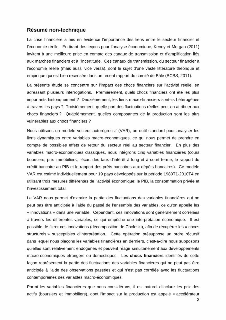
Résumé non-technique
La crise financière a mis en évidence l’importance des liens entre le secteur financier et
l’économie réelle. En tirant des leçons pour l’analyse économique, Kenny et Morgan (2011)
invitent à une meilleure prise en compte des canaux de transmission et d’amplification liés
aux marchés financiers et à l’incertitude. Ces canaux de transmission, du secteur financier à
l’économie réelle (mais aussi vice versa), sont le sujet d’une vaste littérature théorique et
empirique qui est bien recensée dans un récent rapport du comité de Bâle (BCBS, 2011).
La présente étude se concentre sur l’impact des chocs financiers sur l’activité réelle, en
adressant plusieurs interrogations. Premièrement, quels chocs financiers ont été les plus
importants historiquement ? Deuxièmement, les liens macro-financiers sont-ils hétérogènes
à travers les pays ? Troisièmement, quelle part des fluctuations réelles peut-on attribuer aux
chocs financiers ? Quatrièmement, quelles composantes de la production sont les plus
vulnérables aux chocs financiers ?
Nous utilisons un modèle vecteur autorégressif (VAR), un outil standard pour analyser les
liens dynamiques entre variables macro-économiques, ce qui nous permet de prendre en
compte de possibles effets de retour du secteur réel au secteur financier. En plus des
variables macro-économiques classiques, nous intégrons cinq variables financières (cours
boursiers, prix immobiliers, l’écart des taux d’intérêt à long et à court terme, le rapport du
crédit bancaire au PIB et le rapport des prêts bancaires aux dépôts bancaires). Ce modèle
VAR est estimé individuellement pour 19 pays développés sur la période 1980T1-2010T4 en
utilisant trois mesures différentes de l’activité économique: le PIB, la consommation privée et
l’investissement total.
Le VAR nous permet d’extraire la partie des fluctuations des variables financières qui ne
peut pas être anticipée à l’aide du passé de l’ensemble des variables, ce qu’on appelle les
« innovations » dans une variable. Cependant, ces innovations sont généralement corrélées
à travers les différentes variables, ce qui empêche une interprétation économique. Il est
possible de filtrer ces innovations (décomposition de Choleski), afin de récupérer les « chocs
structurels » susceptibles d’interprétation. Cette opération présuppose un ordre récursif
dans lequel nous plaçons les variables financières en derniers, c’est-a-dire nous supposons
qu’elles sont relativement endogènes et peuvent réagir simultanément aux développements
macro-économiques étrangers ou domestiques. Les chocs financiers identifiés de cette
façon représentent la partie des fluctuations des variables financières qui ne peut pas être
anticipée à l’aide des observations passées et qui n’est pas corrélée avec les fluctuations
contemporaines des variables macro-économiques.
Parmi les variables financières que nous considérons, il est naturel d’inclure les prix des
actifs (boursiers et immobiliers), dont l’impact sur la production est appelé « accélérateur

3
financier » (Bernanke, Gertler & Gilchrist, 1999). En effet, les fluctuations des prix des actifs
modifient les bilans financiers des ménages et des entreprises, ce qui peut déterminer leur
accès au crédit en présence d’asymétries informationnelles. Ce canal peut passer par
l’impact sur la valeur nette de l’emprunteur ou sur la valeur des garanties dont il dispose.
Les fluctuations des prix d’actifs peuvent également déterminer l’accès au crédit par leur
impact sur les bilans financiers des banques. Dans ce cas, le canal passe par les effets sur
le levier d’endettement de l’intermédiaire financier ou sur les conditions associées à de
nouveaux apports en capital. Finalement, d’éventuels chocs de confiance pourraient aussi
être capturés par les fluctuations des cours boursiers étant donné leur ajustement rapide aux
nouvelles informations.
Entre les sources possibles de chocs financiers, nous retenons également l’écart entre taux
d’intérêt (à court et à long terme). Les fluctuations de cet écart ont un impact sur les bilans
des banques, dont l’actif et le passif sont composés d’instruments à maturités différentes.
D’ailleurs, des études empiriques indiquent que les modifications de la pente de la courbe de
rendements peuvent servir à anticiper les retournements d’activité économique (e.g. Ang,
Piazzesi & Wei, 2006). Finalement, les mesures du levier financier (rapport crédit/PIB ou
rapport prêts bancaires/dépôts) sont associées plus directement au canal de transmission
par le crédit (Bernanke & Gertler, 1995) et figurent également dans des modèles plus
récents du cycle d’endettement et de la liquidité (e.g. Adrian & Shin, 2009).
Plusieurs conclusions découlent de nos résultats. Premièrement, l’effet des chocs financiers
sur l’activité économique est assez hétérogène entre pays, ce qui est cohérent avec d’autres
résultats dans la littérature. Deuxièmement, l’effet combiné des cinq chocs financiers
identifiés par notre méthode représente une contribution importante aux fluctuations de
l’activité réelle (33% de la variance du PIB à l’horizon de 3 ans, en moyenne à travers les
pays), dépassant celle des chocs de politique monétaire. Troisièmement, entre les différents
chocs financiers, il apparaît que la plus importante contribution aux fluctuations de l’activité
réelle provient des chocs dus aux prix des actifs financiers (les cours boursiers expliquent
12% de la variance du PIB en moyenne et les prix immobiliers 9%). L’écart des taux ou le
levier d’endettement (rapport crédit-PIB ou rapport prêts bancaires-dépôts) contribuent
chacun pour 3 à 4% supplémentaire (en moyenne à travers pays). Quatrièmement, en
général l’effet combiné des cinq chocs financiers est plus important pour les fluctuations de
l’investissement que pour celles de la consommation privée. Cinquièmement, il ressort des
décompositions historiques que la contribution des chocs financiers aux fluctuations de
l’activité est plus importante lors des épisodes associés aux déséquilibres financiers (les
crises mais aussi les périodes de forte expansion). Il est donc possible que l’intensité des
liens macro-financiers varie à travers le temps ou de façon non-linéaire. Cependant, ce
dernier point nécessiterait d’autres méthodes, que nous prévoyons pour des travaux futurs.

4
1. Introduction
The global financial crisis stressed the need to improve our understanding of the links
between the financial sector and the real economy. Kenny and Morgan (2011) highlight the
central role financial shocks played in the crisis and attribute much of the forecasting failures
to inadequate attention paid to “…key transmission and amplification channels, especially
those linked to financial markets and uncertainty.” These channels, both from the financial
sector to the real sector and vice versa, are described in a useful survey of recent theoretical
and empirical work by the Basel Committee on Banking Supervision (BCBS, 2011). Here we
focus on the impact of financial shocks on real activity, but in a framework that allows for
feedback in both directions. We use standard reduced form methods (identified vector auto-
regressions or VARs) to address several relevant questions. First, which financial shocks
have been more important historically? Second, is there heterogeneity across countries in
terms of macro-financial linkages? Third, how much do financial shocks contribute to real
economic fluctuations? Fourth, which components of output are most affected by financial
shocks?
Since we use standard VARs and a country-by-country approach, the underlying
assumptions are that (i) international spillovers are captured by an indicator of foreign
demand for exports, (ii) nonlinearities are negligible, and (iii) parameters are constant
through time. While these simplifications are not meant to be realistic, they make it possible
to consider a relatively wide set of 19 economies (most members of the euro area, the area-
wide aggregate and the main other OECD countries), suggesting a range of answers to our
main questions.
Using the VAR reduced form approach, we define a financial shock as a movement in a
financial variable that is unpredictable from past information (an innovation) and is
uncorrelated with contemporary movements in main macro-economic variables (orthogonal).
For each country, we estimate separate VARs using three different measures of real output:
GDP, private consumption or total investment. Each VAR also includes a consumer price
index, short-term interest rates, an international index of commodities prices and an indicator
of foreign demand. VAR models based on this set of variables have become a standard tool
to capture macro-economic dynamics (Christiano et al. 1999). Structural shocks can be
identified using short-term restrictions, long-term restrictions, sign restrictions or a
combination of these. Below, we rely on short-term restrictions using the standard Choleski
decomposition of the innovation covariance matrix, which implies a recursive exogeneity
structure among the variables (see discussion below and details in appendix). Similar
methods have been applied to study the transmission of monetary policy in euro area

5
aggregates (e.g. Peersman & Smets, 2001) as well as in individual euro area countries (e.g.
Mojon & Peersman, 2001).
In principle, a macro-economic VAR can correspond to the reduced form of a general class
of dynamic stochastic general equilibrium (DSGE) models. However, Fernandez-Villaverde
et al. (2007) show that not every DSGE will have a VAR representation (and the opposite is
also true). Kilian (2011) also warns that caution is required in comparing structural VAR and
DSGE results, but both these studies conclude that VAR and DSGE approaches can be
complementary. Since a given VAR can be compatible with a whole class of DSGE models,
VARs are especially useful when there is uncertainty about the most appropriate DSGE
specification, as is the case in the relatively new field of modelling macro-financial linkages.
We augment each VAR to also include five different financial variables: two asset prices
(real house prices and real stock prices), the term spread (difference between long and
short-term interest rates), and two leverage indicators (ratio of private sector credit to GDP
and ratio of aggregate loans to aggregate deposits in the banking sector). The inclusion of
asset prices is natural, given their impact on output through the financial accelerator
(Bernanke, Gertler & Gilchrist, 1999). Changes in asset prices can act through borrowers’
balance sheets, by affecting their net worth or collateral values, but also through banks’
balance sheets, by affecting their leverage and their ability to raise new capital. Since stock
prices adjust rapidly to incorporate new information, they may also capture confidence
shocks. Changes in the term spread (between short- and long-term interest rates) also affect
bank balance sheets, given the maturity mismatch between assets and liabilities. The term
spread also links to a separate literature on the slope of the yield curve as a predictor of
economic activity (e.g. Ang, Piazzesi & Wei, 2006). Finally, the leverage indicators may
capture credit channel effects (Bernanke & Gertler, 1995) more directly than asset prices.
They also figure in models of liquidity and the leverage cycle (e.g. Adrian & Shin, 2009).
Several other financial variables could have been considered but were eliminated because
data was only available for a shorter sample or a more limited set of countries. It is also
difficult to include more than five financial variables in a macro-economic VAR given limited
degrees of freedom. Therefore we do not consider credit spreads across different classes of
borrowers, sovereign spreads across different countries, non-performing loans, loan-loss
provisions or other measures of liquidity or volatility. Still, we consider a sufficiently broad set
of financial variables to benefit from several advantages. First, we can allow for possible
interactions between financial variables as well as between real and financial variables.
Second, the set of five different financial variables allows us to better identify innovations as
fluctuations that are unpredictable from a larger information set. Third, joint analysis of
several financial variables (especially including both house prices and credit) is important

6
given the finding by Borio & Lowe (2002, 2004) that financial imbalances are better identified
through a combination of different financial indicators.
There exists a growing literature extending the standard macroeconomic VAR to incorporate
financial variables.2 The analysis below extends this in three directions. First, as mentioned
above, we simultaneously include five different financial variables. Among the studies cited
in the footnote, only Abildgren (2010) includes more than three financial variables. Second,
we provide a broader cross-country perspective, repeating the exercise for each of 19
industrialised economies (including euro area aggregate data) with consistent samples and
data definitions. Among the studies cited, only three are comparable in country coverage:
Chirinko et al. (2004) consider 13 economies, Assenmacher-Wesche & Gerlach (2008)
consider 17 economies and Fornari & Stracca (2010) consider 21 advanced economies.
However, these authors only include two or three financial variables. Third, we use a longer
sample period to capture a greater number of financial imbalance episodes, starting in
1980Q1 and ending in 2010Q4, which includes the global financial crisis. Again, only
Abildgren (2010) uses a longer sample, but limited to a single country (Denmark).
As is well known, shock identification by the standard Choleski decomposition3 of the
innovation covariance matrix assumes a recursive exogeneity structure that is explicit in the
ordering of the variables in the VAR. At the top of this ordering, we place place the two
external variables (a country-specific foreign demand indicator4 and an international
commodities price index), treating them as more exogenous. These are followed by
domestic output, inflation and interest rates, a fairly standard sequence in the literature going
back to Christiano et al. (1999). The five financial variables are placed lower in the ordering,
allowing them to react to contemporaneous shocks in all the macro-economic variables.
Assenmacher-Wesche & Gerlach (2008) argue that financial variables should follow interest
rates because monetary policy only reacts to asset price movements if these are prolonged,
while asset prices react immediately to changes in monetary policy. The exact ordering
2 For example, Iacoviello (2002), Giuliodori (2005), Neri (2004), Adalid & Detken (2007), den Haan et
al. (2007), Goodhart & Hofmann (2008), Chirinko et al. (2008), Assenmacher-Wesche & Gerlach
(2008), Baumeister et al. (2008), Musso et al. (2010), Giannone et al. (2010), Abildgren (2010) and
Fornari & Stracca (2011). Most of these studies focus on monetary policy transmission.
3 This is also implemented by Giuliodori (2005), Adalid & Detken (2007), Goodhart & Hofmann (2008),
Assenmacher-Wesche & Gerlach (2008), Abildgren (2010) and Musso et al. (2010). See appendix.
4 For EU27 countries this was drawn from the Eurosystem BMPE trade consistency exercise. For
non-EU countries it was constructed as a weighted average of real imports of trading partners, with
the trade weights used to calculate effective exchange rates at the ECB.

7
within the block of financial variables is less clear-cut. We follow the suggestion by Goodhart
& Hofmann (2008) that house prices should appear first among the financial variables
because they are probably stickier. We place the leverage indicators last among the
financial variables as do Adalid & Detken (2007), Goodhart & Hofmann (2008) and Musso,
Neri & Stracca (2010). These authors argue that this ordering implies a conservative
approach to the endogeneity of money and credit growth, allowing them to react
contemporaneously to shocks in all the other endogenous variables5.
All VARs were estimated with two lags6 of each of ten endogenous variables. The estimation
sample usually7 covered 1981Q2 to 2010Q4. With the exception of interest rates, the term
spread, the loans-to-deposits ratio and the loans-to-GDP ratio (expressed as a “credit
growth” indicator8), all variables are expressed in log-levels and seasonally adjusted. As also
observed in other studies, the credit data from the IMF International Financial Statistics suffer
from level shifts, so these were eliminated using the TRAMO software package before
calculating the leverage ratios.
2. 3.1. How much do financial shocks explain?
The forecast error variance decompositions from the VARs serve as a natural tool to
compare the relative importance of different shocks across countries with different output
volatility. Three results stand out. First, the contribution of financial variables to real
fluctuations is fairly heterogeneous across countries (confirming findings in Chirinko et al.
2008). Second, the combined contribution from the five financial shocks is surprisingly high
(33% of GDP variance at the 3-year horizon, averaging across countries) and it increases
with the horizon (see Table 1 below). Third, among the financial shocks (see Table 2 for
details), those to asset prices appear to contribute more to real fluctuations.
Averaging across countries, shocks to real stock prices contribute more than 12% of output
variance at the 3-year horizon, shocks to real house prices contribute 9%, shocks to the term
5 Our results are robust to alternative orderings of the financial variables. Since there are five of these
variables, there are 5!=120 possible orderings. For each estimated VAR, all 120 variance
decompositions were generated. Results in the text are close to the average across these 120
decompositions. See appendix for standard deviations across the 120 decompositions.
6 Considering up to 5 lags, the Schwarz Bayesian Information Criterion favours only 1 lag in all cases.
7 For Italy, Denmark, Japan and New Zealand, our quarterly house price series ends in 2010Q3.
Loans data for Canada ends in 2008Q4. See appendix for the exact estimation sample for each VAR.
8 See Biggs, Mayer & Pick (2009). Our main conclusions are unaffected by using their “credit impulse”
indicator instead.

8
spread 5%, and shocks to the leverage ratios around 3%-4% each. However, this ranking of
financial shocks is uncertain as differences are often small and may be insignificant. In
addition, the ranking varies across countries, reflecting different institutional features and
financial structures (see discussion in Assenmacher-Wesche & Gerlach, 2008). These
institutional features may either dampen or amplify the impact of financial shocks on the
behaviour of household and firms (see Bernanke & Gertler, 1995).
Table 1 is divided in separate panels for GDP, Private Consumption and Gross Fixed Capital
Formation. Each panel reports the share of forecast variance explained at different horizons
by the combined contribution of shocks to the five financial variables considered (real house
prices, real stock prices, long-short spread, loans-to-GDP ratio and loans-to-deposit ratios).
For GDP, the cumulative contribution of the five financial shocks appears to be clearly higher
for Germany, Spain, and the Netherlands in the euro area, and Australia, Denmark and
Sweden outside. For Private Consumption, the cumulative contribution is again highest for
Germany and Spain in the euro area, followed by the Netherlands and Ireland. Outside the
euro area, the combined contribution is highest in Denmark, Canada and New Zealand. For
Investment, the cumulative contribution of financial shocks is highest for Spain, Finland and
Ireland in the euro area, and for New Zealand, Sweden, Denmark and Australia outside.
Table 1: % of forecast variance explained by combined effect of five financial shocks
BE DE ES FI FR IE IT LU NL EA DK GB SE AU CA CH US JP NZ AVG
Gross Domestic Product
1y 28 36 35 29 25 18 14 14 32 35 23 24 32 32 18 14 23 16 27 25.0
2y 35 45 39 36 32 29 19 18 40 37 34 27 34 40 24 27 26 30 34 31.9
3y 34 44 39 36 37 30 20 19 39 40 40 25 37 43 31 25 29 32 35 33.4
6y 34 45 40 39 37 32 21 19 39 43 39 30 39 43 34 26 29 34 37 34.7
Private Consumption
1y 3 29 39 11 13 17 7 8 15 4 29 14 11 16 29 14 12 19 29 16.7
2y 11 40 45 19 21 35 16 22 27 11 35 15 13 26 29 19 20 25 36 24.4
3y 13 41 46 24 26 36 20 25 33 17 39 16 16 27 30 21 24 28 36 27.3
6y 16 42 48 27 30 38 23 27 38 23 39 20 17 28 38 22 27 31 37 30.1
Gross Fixed Capital Formation
1y 3 17 30 23 15 25 17 13 18 20 20 19 37 31 7 17 20 9 44 20.4
2y 14 22 43 41 25 38 30 18 31 30 33 29 44 34 15 25 29 25 53 30.5
3y 17 24 42 43 26 40 32 18 33 39 38 28 43 37 18 26 34 31 55 32.9
6y 18 25 43 47 30 50 35 19 34 45 38 31 44 38 23 27 34 36 56 35.3
Note: see appendix 1 for country codes

9
Focussing on the (unweighted) cross-country average in the final column, the combined
contribution of the five financial variables appears to be slightly higher for GDP than for
investment and is lower for consumption at all horizons. Looking across countries, there is
no clear pattern, with the combined contribution sometimes similar across measures of
output and sometimes very dissimilar. For some countries financial shocks contribute more
to fluctuations in consumption and for others to those in investment or GDP.
At first sight, it may seem surprising that three countries known for their large financial sector
(Switzerland, Luxembourg, United Kingdom) appear to be among the less vulnerable to
financial shocks. There are several explanations for this result. First, these three countries
export much of the financial services they produce. In so far as financial shocks originate (or
propagate) abroad, they may affect foreign demand for these services within the same
quarter. Given the ordering in the Choleski decomposition, such a shock will then be
classified as a foreign demand shock rather than a financial shock (foreign financial shocks
are foreign shocks first and financial shocks second). Furthermore, to focus on the link
between domestic lending and domestic activity, the leverage ratios were constructed using
bank loans to the domestic private sector.
Second, most of the financial shocks considered (house price shocks, stock price shocks
and shocks to the term spread) can affect household and firm decisions directly even in the
absence of a banking sector. As observed by Bernanke and Gertler (1995), the credit
channel is an amplification mechanism, not really a separate channel.
Finally, the variance decomposition normalises output volatility of different countries (in
Ireland or Luxembourg it is 8 to 10 times larger than in France, Germany or the euro area),
but important differences remain within the decomposition (Figure 3.1). In Luxembourg and
Switzerland the own-shock (exogenous) contribution to GDP growth is much higher. This
may reflect higher measurement error, since in smaller economies idiosyncratic shocks to
individual sectors or even firms are more likely to distort aggregate measures. On the other
hand, the United Kingdom ranks first in terms of the contribution from foreign shocks,
consistent with its status as a larger open economy. Therefore the smaller contribution of
financial shocks in these three countries partly reflects the larger role of exogenous or
external factors in driving their GDP.
Another puzzling result is that Germany appears to have the highest combined contribution
from financial shocks. In part this is explained by the observation above: adjusting for its
higher contribution from external shocks, Germany falls five places in the ranking. Germany
also stands out because its contribution of financial shocks is much higher for private
consumption than for investment (where the contribution actually falls below the cross-
country average). This is consistent with the common view that German industry is largely

10
composed of smaller firms that finance their investment through long-standing banking
relationships that insulate them from shocks. On the other hand, private consumption
fluctuations in Germany appear to be largely driven by real house price shocks (see below).
Figure 1: GDP (% of variance explained after 3 years)
0
20
40
60
80
100
BE DE ES FIFR IE IT LU NL EA DK GB SE AU CA CH US JP NZ
House prices Stock prices Long-short spread Loans/GDPLoans/Deposits External Macro
As reported in Figure 1, the relative contribution of individual financial shocks varies
significantly across countries. This figure reports the forecast error decomposition for Gross
Domestic Product at the 3-year horizon. At the bottom of the graph are the financial
variables: real house prices (blue bars), real stock prices (red bars) long-short term spread
(green), bank loans to GDP ratio (orange) and bank loans to deposits ratio (purple). Above
this appear the combined contributions from external variables (light yellow bars), meaning
the country-specific foreign demand indicator and the international commodities price index.
Finally, at the top of the graph appear the combined contributions from domestic
macroeconomic variables (grey bars), which include the own-shock to GDP, as well as
shocks to consumer prices, and short term interest rates.
The contribution from the own-shock to GDP reflects the exogenous component in output
movements. This may be exaggerated by omitted variable bias and the particular
identification scheme chosen (since output is ordered first among domestic variables, the
own-shock will absorb any shocks to other domestic and financial variables that are
contemporaneously correlated with those in output). On the other hand, since the financial
variables appear last in the Choleski ordering (at the bottom of the graph) it is natural that
they contribute relatively less to output fluctuations (they are only the residual component of

11
innovations after accounting for correlation with contemporaneous shocks in all variables
higher in the ordering). This “limitation” of our identification scheme suggests that our results
only provide a lower bound estimate for the contribution of financial shocks to output
fluctuations, emphasising the fact that they are estimated to be surprisingly large.
Table 2 reports the forecast variance decomposition at the 3-year horizon by financial shock.
Real house price shocks explain more GDP fluctuations in Germany (22%), Spain (18%) and
Ireland (16%). Real stock price shocks affect GDP most in Sweden (23%), Japan (20%),
Australia (19%), the Netherlands (14%), and Spain (13%). Shocks to the term spread
explain more GDP fluctuations in the euro area aggregate (14%), France (11%), and the US
(9%). Shocks to credit growth are more important in Switzerland (12%), France (11%) and
Denmark (6%). Shocks to the loans-to-deposits ratio account for more GDP fluctuations in
Belgium (12%), the Netherlands (6%), and Japan (4%).
In the final column of Table 2, the cross-country average suggests that asset price shocks
contribute much more than the other financial variable shocks. This may not be surprising,
given that credit aggregates are determined jointly by supply and demand, with credit
Table 2: % of forecast variance at 3-yr horizon explained by individual financial shocks
BE DE ES FI FR IE IT LU NL EA DK GB SE AU CA CH US JP NZ AVG
Gross Domestic Product
House prices 6 22 18 9 7 16 1 4 8 12 11 5 5 15 13 1 3 7 12 9.2
Stock prices 9 10 14 15 7 8 11 10 14 8 12 14 23 19 7 9 10 20 14 12.4
Term spread 3 8 3 4 11 1 4 0 8 14 8 1 4 2 4 1 9 1 1 4.6
Loans/GDP 3 2 2 5 11 2 0 1 2 5 6 4 3 3 4 12 4 1 5 3.9
Loans/deposits 12 1 3 3 0 4 3 4 6 2 3 2 2 3 3 3 2 4 3 3.3
Private Consumption
House prices 3 18 14 6 10 25 2 2 0 9 7 6 3 15 15 2 1 5 11 8.0
Stock prices 2 10 15 5 3 5 8 11 12 0 20 9 8 6 4 5 5 15 11 8.2
Term spread 7 5 12 1 7 0 2 2 4 1 1 1 1 2 5 6 10 1 2 3.6
Loans/GDP 0 7 1 4 1 5 1 6 16 3 4 0 1 2 4 5 6 4 11 4.3
Loans/deposits 2 1 4 8 5 2 6 4 1 4 7 1 3 1 2 4 3 3 1 3.1
Gross Fixed Capital Formation
House prices 2 12 12 21 10 19 11 6 5 14 19 4 7 13 8 1 3 3 24 10.2
Stock prices 1 4 19 8 6 13 5 7 8 6 7 12 31 14 2 9 9 17 16 10.3
Term spread 8 1 7 6 4 1 4 1 10 2 6 3 3 5 1 0 7 1 3 3.8
Loans/GDP 0 5 3 2 6 4 6 2 6 16 2 0 1 1 2 8 12 3 6 4.4
Loans/deposits 6 2 1 5 1 3 7 2 4 1 3 8 1 4 5 8 3 8 5 4.1

12
demand containing “a significant countercyclical component” (Bernanke & Gertler, 1995).
Among asset prices, real stock price shocks appear to contribute more on average than real
house price shocks, although this is not the case in all countries. In fact, for Germany and
Ireland the contribution of house prices is nearly twice that of stock prices, and it is also
higher in Spain, Canada and the euro area aggregate. There is no a priori reason why
house price shocks or stock price shocks should contribute more. This will depend on
several characteristics of the economy under question, including the structure of firm and
household finance9, the relative size of stock-market capitalisation and mortgage debt, the
distribution of stock ownership among households, corporations and non-residents.
Institutional features of the housing market will also matter, such as the typical loan-to-value
ratio, use of fixed or variable mortgage rates, typical mortgage duration in years, mortgage
equity withdrawal possibilities and role of state mortgage companies10.
Focussing on the euro area aggregate and the US, GDP fluctuations in the former are more
sensitive to shocks to the term spread (13.8%) and real house prices (12%), followed by
shocks to real stock prices (7.5%), to credit growth (4.7%) and to the loans-to-deposits ratio
(2.2%). In the US, real stock prices tops the ranking (10.2%) followed by the term spread
(9%), credit growth (4.4%), real house prices (3%), and the loans-to-deposits ratio (2.3%).
In the middle panel of Table 3.2, when Private Consumption replaces GDP in the VAR as the
indicator of economic activity, the leverage indicators for euro area countries were calculated
using long series on loans to households provided by the ECB11. Starting with real house
price shocks, their contribution to fluctuations in private consumption is highest in Ireland
(24%), Germany (18%), Australia (15.4%), Canada (14.6%) and Spain (14%). Real stock
price shocks contribute most to consumption fluctuations in Denmark (20%), Japan (15%)
and Spain (14.6%). Shocks to the term spread contribute more to consumption fluctuations
in Spain (12%), the US (10%), Belgium and France (both 7%). Shocks to credit growth
contribute most in the Netherlands (16%), New Zealand (11%) and Germany (7%). Shocks
to the loans-to-deposits ratio contribute most in Finland (8%), Denmark (7%), and Italy
(6.5%).
For euro area aggregate data, fluctuations in consumption are explained more by shocks to
real house prices (9%), to the loans-to-deposits ratio (4%), and to credit growth (3%).
9 See ECB (2007) and ECB (2009).
10 See Calza et al (2009), ECB (2009) and CGFS (2006).
11 This may reduce the comparability of results for euro area countries to those for other countries, and
also to euro area country results in the VARs using GDP, which used IMF data on loans.

13
Shocks to the term spread (0.6%) or to real stock prices (0.5%) are less important. By
contrast, in the US consumption fluctuations are explained more by shocks to the term
spread (10%), to credit growth (6%), and to real stock prices (5%), than by shocks to the
loans-to-deposits ratio (3%) or to real house prices (0.6%).
The bottom panel of Table 2 provides the variance decomposition at the 3-year horizon when
Investment replaces GDP in the VAR as the measure of economic activity. In this case, for
euro area countries the leverage indicators are calculated using loans to non-financial
corporations. Shocks to real house prices make the largest contribution to investment
fluctuations in New Zealand (24%), Finland (21%), Ireland (19%) and Denmark (18.6%). The
contribution of house price shocks in Spain is above average at 12%. Shocks to real stock
prices appear to have a much larger role in Sweden (31%) and Germany (19%), followed by
Japan (17%) and New Zealand (16.5%). Shocks to the term spread contribute more to
investment fluctuations in the Netherlands (10%), Belgium (8%), the US (7%) and Spain
(6.5%). Shocks to credit growth have the largest effects on investment in the euro area
aggregate (16%), the US (12%), Switzerland (8%) and Italy (6%). Shocks to the loans-to-
deposits ratio contribute more to investment fluctuations in the United Kingdom (8.5%)
Switzerland (8.2%), Japan (7.6%) and Italy (6.8%).
For the aggregate euro area data, fluctuations in investment are affected more by shocks to
credit growth (16%), followed by real house price shocks (14%), real stock price shocks
(6%), shocks to the term spread (2%) and to the loans-to-deposits ratio (1%). For the US,
investment fluctuations are also more sensitive to credit growth shocks (12%), followed by
real stock price shocks (8%), shocks to the term spread (7%), to real house prices (2.7%)
and to the loans-to-deposits ratio (2.6%).
3. When were financial shocks important?
While the forecast error variance decomposition provided an indication of the relative
importance of financial shocks for output growth, historical decompositions can provide an
indication of when in the sample those shocks were most present. In the figures below, euro
area and US GDP growth are decomposed into the contributions of three groups of
variables. The blue bars represent the contribution of shocks to the macro-economic
variables (GDP, inflation and interest rates). The red bars represent the combined
contribution of the five financial variables and the green bars represent the contribution of the
external variables (foreign demand and commodities prices).
Contributions to GDP growth were calculated by recovering the residuals (innovations) from
each equation, transforming these to structural shocks by multiplying by the Choleski factor
and then using the resulting shocks at each point in time to scale the impulse response

14
functions forward to the end of the sample. These impulses from shocks at different periods
were then summed at each point in the sample so that the effect of the current shock and all
past shocks were combined to obtain the contribution to growth from that particular kind of
shock.
Only the historical decompositions for the euro area and the US are discussed below. The
historical decompositions for other countries appear in the appendix.
Figure 2: Euro Area GDP growth Historical Decomposition
-10%
-8%
-6%
-4%
-2%
0%
2%
4%
82 84 86 88 90 92 94 96 98 00 02 04 06 08 10
Financial variables contribution to GDP growthMacro variables contribution to GDP growthExternal variables contribution to GDP growth
For the euro area, the contributions from financial variable shocks were limited in the early
1980s and tended to be positive following the peak in the US dollar associated with the Plaza
accord. The positive contributions picked up in 1989Q2-1990Q3 during the house price
boom. The financial shock contributions turned negative in 1991 and plunged through the
ERM crisis of September 1992 and the ensuing recession. From 1995 to 1999 the
contribution to growth from financial shocks was limited, but it gained consistency during the
“new technology” stock market bubble from 1999Q4 peaking in 2000Q3. In 2001 the stock
market bubble burst and contributions fell to zero. There is another string of positive
contributions starting in 2004Q2 when real house prices boomed and lasting until the first
signs of financial turmoil in 2007Q2. The contribution turned negative in 2007Q3 and
plunged until 2009Q2 as GDP collapsed. The negative contribution to growth from financial
shocks diminished until 2010, when they remained mildly negative.
15
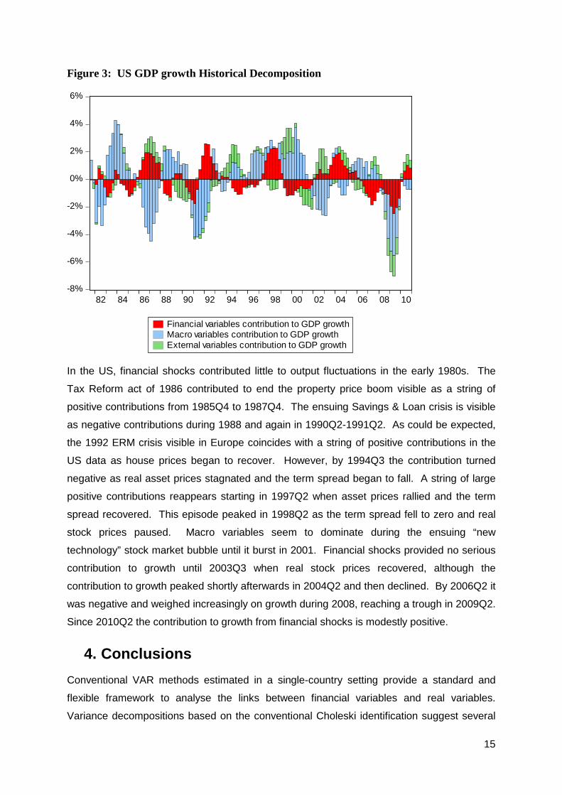
Figure 3: US GDP growth Historical Decomposition
-8%
-6%
-4%
-2%
0%
2%
4%
6%
82 84 86 88 90 92 94 96 98 00 02 04 06 08 10
Financial variables contribution to GDP growthMacro variables contribution to GDP growthExternal variables contribution to GDP growth
In the US, financial shocks contributed little to output fluctuations in the early 1980s. The
Tax Reform act of 1986 contributed to end the property price boom visible as a string of
positive contributions from 1985Q4 to 1987Q4. The ensuing Savings & Loan crisis is visible
as negative contributions during 1988 and again in 1990Q2-1991Q2. As could be expected,
the 1992 ERM crisis visible in Europe coincides with a string of positive contributions in the
US data as house prices began to recover. However, by 1994Q3 the contribution turned
negative as real asset prices stagnated and the term spread began to fall. A string of large
positive contributions reappears starting in 1997Q2 when asset prices rallied and the term
spread recovered. This episode peaked in 1998Q2 as the term spread fell to zero and real
stock prices paused. Macro variables seem to dominate during the ensuing “new
technology” stock market bubble until it burst in 2001. Financial shocks provided no serious
contribution to growth until 2003Q3 when real stock prices recovered, although the
contribution to growth peaked shortly afterwards in 2004Q2 and then declined. By 2006Q2 it
was negative and weighed increasingly on growth during 2008, reaching a trough in 2009Q2.
Since 2010Q2 the contribution to growth from financial shocks is modestly positive.
4. Conclusions
Conventional VAR methods estimated in a single-country setting provide a standard and
flexible framework to analyse the links between financial variables and real variables.
Variance decompositions based on the conventional Choleski identification suggest several

16
conclusions. First, the contribution of financial variables to real fluctuations is fairly
heterogeneous across countries. Second, on average across countries, this contribution is
rather large (up to 33% of GDP variance at the 3-year horizon) and exceeds the contribution
of monetary policy shocks. Third, shocks to real asset prices (house prices and stock prices)
often have greater real effects than those to the term spread or to leverage (loans-to-GDP
ratio or loans-to-deposits ratio). Fourth, comparing GDP, private consumption or investment,
the latter is often most responsive to financial shocks. However, our results suggest that for
some countries financial shocks may affect consumption more strongly than investment.
When introducing financial frictions in DSGE models, the modelling of firm and household
decisions should reflect country-specific characteristics.
Our main conclusions are robust to several changes in specification (see appendix),
including estimating the VAR with longer lags, using log-levels instead of year-on-year
growth rates, and dropping the volatile periods at the start and end of the estimation sample.
When we re-estimate our VARs with other specifications or using only subsamples, shocks
to asset prices continue to contribute more to real fluctuations (on average across countries).
We have also checked the robustness of our results to alternative orderings of the financial
variables (see appendix); however, the Choleski identification scheme does assume that
within the same observation period shocks to a given variable are orthogonal to those of
variables placed higher in the ordering. This assumption is clearly more appropriate at
monthly frequency than at the quarterly frequency that we adopt in order to use national
accounts data. In fact, Gilchrist et al. (2009) use monthly data and find a higher contribution
of financial shocks to real fluctuations. They identify credit shocks in the US corporate bond
market that account for up to 30% of the variability of monthly employment and industrial
production at the 2-4 year horizon.
We should draw attention to several limitations of our analysis. First, we use a longer
sample than in many previous studies in order to include as many financial imbalance
episodes as possible, but this also increases the number of potential regime shifts (such as
EMU). In addition, there may be theoretical reasons to expect the relation between real and
financial variables to vary at different points in the business cycle. Both these remarks
suggest that methods allowing for time-varying parameters may be more appropriate.
Second, our approach ignores possible cross-country spillovers that could be captured by
panel VAR methods (e.g. Ciccarelli, Ortega & Valderrama, 2012). Finally, our standard VAR
framework is only a linear approximation to the data, while the relation between real and
financial variables may be subject to nonlinearities (e.g. Hartmann et al 2012).

17
References
Abildgren, Kim (2010) “Business cycles, monetary transmission and shocks to financial
stability,” Danmarks Nationalbanken WP 2010/71.
Adalid, Ramón & Carsten Detken (2007) “Liquidity shocks and asset price boom/bust cycles”
European Central Bank WP 732.
Adrian, Tobias & Hyun-Song Shin (2006) “Liquidity and leverage,” Journal of Financial
Intermediation, 1, pp.418-437.
Ang, Andrew, Monika Piazzesi & Min Wei (2006) “What does the yield curve tell us about
GDP growth?” Journal of Econometrics, 131:359-403-
Assenmacher-Wesche, Katrin & Stefan Gerlach (2008) "Financial structure and the impact of
monetary policy on asset prices," Working Paper 2008-16, Swiss National Bank (also CEPR
Discussion Paper 6773).
Basel Committee on Banking Supervision (BCBS) (2011) “The transmission channels
between the financial and real sectors: a critical survey of the literature,” Bank for
International Settlements Working Paper 18.
Baumeister, Christiane, Eveline Durinck & Gert Peersman (2008) “Liquidity, inflation and
asset prices in a time-varying framework for the euro area,” National Bank of Belgium
Working Paper 142.
Bernanke, Ben & Mark Gertler (1996) “Inside the black box: the credit channel of monetary
transmission,” Journal of Economic Perspectives, 9(4):27-48.
Bernake, Ben, Mark Gertler & Simon Gilchrist (1999) “The financial accelerator in a
quantitative business cycle framework,” chapter 21 in J.B. Taylor and M. Woodford (eds.)
Handbook of Macroeconomics, Elsevier Science, volume I, pp.1341-1393.
Biggs, Michael, Thomas Mayer & Andreas Pick (2009) “Credit and Economic Recovery,” De
Nederlandsche Bank Working Paper 218/2009.
Borio, Claudio & Philip Lowe (2002) “Asset prices, financial and monetary stability: exploring
the nexus,” Bank for International Settlements Working Paper 114.
Borio, Claudio & Philip Lowe (2004) “Securing sustainable price stability: should credit come
back from the wilderness?” Bank for International Settlements Working Paper 157.
Calza, Alessandro, Tommaso Monacelli & Livio Stracca (2009) “Housing finance and
monetary policy,” ECB Working Paper 1069.
Canova, Fabio & Evi Pappa (2007) “Price differentials in monetary unions: the role of fiscal
shocks,” Economic Journal, 117:713-737.

18
Chirinko, Robert S., Leo de Haan & Elmer Sterken (2008) "Asset price shocks, real
expenditures, and financial structure: a multi-Country Analysis," CESifo Working Paper
Series 2342.
Christiano, Lawrence J., Martin Eichenbaum & Charles L. Evans (1999) “Monetary policy
shocks: What have we learned and to what end?” Chapter 2 in J.B. Taylor and M. Woodford
(eds.) Handbook of Macroeconomics, Elsevier Science, volume I, pp.65-148.
Ciccarelli, Matteo, Eva Ortega & Maria Teresa Valderrama (2012) “Heterogeneity and cross-
country spillovers in global macro-financial linkages,” mimeo, ECB.
Committee on the Global Financial System (2006) “Housing finance in the global financial
market,” CGFS papers 26.
Den Haan, Wouter J., Steven W. Sumner and Guy M. Yamashiro (2007) “Bank loan
portfolios and the monetary transmission mechanism,” Journal of Monetary Economics,
54:904-924.
European Central Bank (2009) “Housing finance in the euro area,” Occasional Paper 101.
European Central Bank (2007) “Corporate finance in the euro area,” Occasional Paper 63.
Faust, Jon & Eric Leeper (1997) “When do long-run identifying restrictions give reliable
results?” Journal of the American Statistical Association, 15(3), pp.345-353.
Fernandez-Villaverde, Jesús, Juan F.Rubio-Ramírez, Thomas J. Sargent and
Mark W. Watson (2007) “ABCs (and Ds) of Understanding VARs,” American Economic
Review, 97:1021-1028.
Fornari, Fabio & Livio Stracca (2011) “The Minsky moment: Do financial shocks matter?”
mimeo ECB, presented at Economic Policy 55th panel meeting, Budapest 15-16 April 2011.
Giannone, Domenico, Michele Lenza & Lucrezia Reichlin (2010) “Money, credit, monetary
policy and the business cycle in the euro area,” in Papademos, L. and J. Stark (eds.)
Enhancing Monetary Analysis, Frankfurt: European Central Bank.
Gilchrist, Simon, Vladimir Yankow & Egon Zakrajsek (2009) “Credit market shocks and
economic fluctuations: evidence from corporate bond and stock markets,” Journal of
Monetary Economics, 56:471-493.
Giuliodori, Massimo (2005) "The role of house prices in the monetary transmission
mechanism across European countries," Scottish Economic Society, vol. 52(4), pp.519-543
(also DNB WP015).
Goodhart, Charles & Boris Hofmann (2008) "House prices, money, credit and the macro-
economy" Oxford Review of Economic Policy, 24(1), pp.180-205 (also ECB WP 888).

19
Hartmann, Philipp, Kirstin Iacoviello, Matteo (2002) "House prices and business cycles in
Europe: a VAR analysis," Boston College Working Papers in Economics 540, Boston College
Department of Economics (also ECB WP 18)
Kenny, Geoff and Julian Morgan (2011) “Some lessons from the financial crisis for the
economic analysis,” European Central Bank Occasional Paper 130.
Kilian, Lutz (2011) “Structural Vector Autoregressions,” CEPR Discussion Paper 8515.
Mojon, Benoit & Gert Peersman (2001) “A VAR description of the effects of monetary policy
in the individual countries of the euro area,” European Central Bank WP 092.
Musso, Alberto, Stefano Neri & Livio Stracca (2010) “Housing, consumption and monetary
policy: How different are the US and the euro area?” European Central Bank WP 1161.
Neri, Stefano (2004) "Monetary policy and stock prices: theory and evidence," Temi di
discussione, Bank of Italy, 513, Economic Research Department.
Peersman, Gert & Frank Smets (2001) “The monetary transmission mechanism in the euro
area: more evidence from VAR analysis,” European Central Bank WP 091.

20
Appendix 1: Structural VAR identification by short -run restrictions
Let yt, t= 1,…,T denote a K-dimensional vector of variables. This can be approximated by a
vector autoregression of finite order p with the following structural form:
B0yt = B1yt-1 + … + Bpyt-p + ut
Where ut denotes a mean zero serially uncorrelated error term, also known as structural
innovation or structural shock. The error term is usually assumed to be unconditionally
homoskedastic (constant variance). Constants and deterministic trends have been
suppressed for notational convenience. This structural form can be expressed compactly as
B(L)yt-1 = ut
Where L denotes the lag operator (Lyt = yt-1) and B(L) = B0 – B1L – B2L2 - … - BpL
p is the
autoregressive lag polynomial of order p. The standard normalization of the variance-
covariance of the structural error term is
E(utut´) = Σu = IK
Meaning (i) there are as many structural shocks as variables in the model, (ii) these shocks
are mutually uncorrelated so that Σu is diagonal and (iii) the variance of all structural shocks
is equal to unity. The latter normalization involves no loss of generality as long as the
diagonal elements of B0 are unrestricted.
The reduced form representation of the model is required for estimation, expressing yt as a
function of lagged yt only. Premultiplying both sides of the structural form by B0-1,
B0-1B0yt = B0
-1B1yt-1 + … + B0-1Bpyt-p + B0
-1ut
So the reduced form can be written
yt = A1yt-1 + … + Apyt-p + εt where Ai = B0-1Bi, i = 1,…,p and εt = B0
-1ut
Equation-by-equation ordinary least squares regression provides consistent estimates of the
reduced form parameters Ai, reduced form errors εi and their covariance matrix E(εtεt´) = Σε.
However, since the reduced form errors are εt = B0-1ut they are likely to be mutually
correlated (Σε ≠ IK). An estimate of B0-1 is required to recover the orthogonal structural
shocks (ut) from the correlated reduced form errors (εt). The most common approach is to
assume a recursive structure, applying the Choleski decomposition to the covariance matrix
Σε of the estimated residuals to obtain the lower triangular K x K matrix P such that
PP´ = Σε
Assuming P = B0-1 we can recover the structural shocks as ut = P-1εt
21
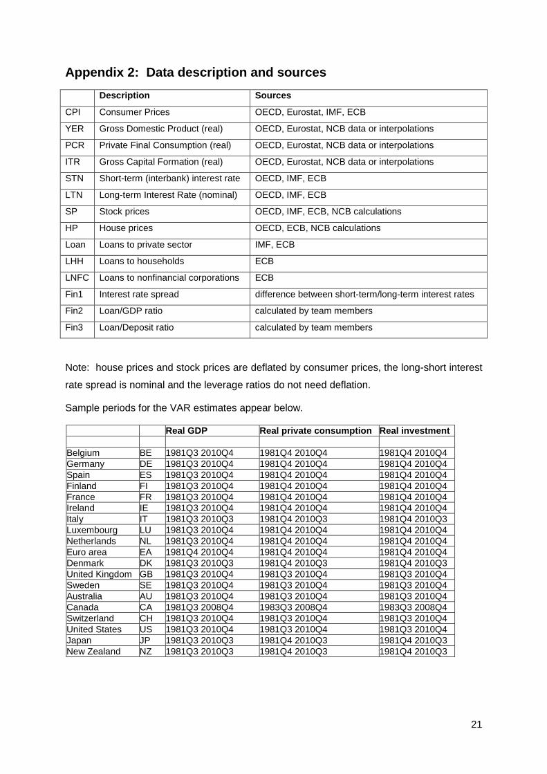
Appendix 2: Data description and sources
Description Sources
CPI Consumer Prices OECD, Eurostat, IMF, ECB
YER Gross Domestic Product (real) OECD, Eurostat, NCB data or interpolations
PCR Private Final Consumption (real) OECD, Eurostat, NCB data or interpolations
ITR Gross Capital Formation (real) OECD, Eurostat, NCB data or interpolations
STN Short-term (interbank) interest rate OECD, IMF, ECB
LTN Long-term Interest Rate (nominal) OECD, IMF, ECB
SP Stock prices OECD, IMF, ECB, NCB calculations
HP House prices OECD, ECB, NCB calculations
Loan Loans to private sector IMF, ECB
LHH Loans to households ECB
LNFC Loans to nonfinancial corporations ECB
Fin1 Interest rate spread difference between short-term/long-term interest rates
Fin2 Loan/GDP ratio calculated by team members
Fin3 Loan/Deposit ratio calculated by team members
Note: house prices and stock prices are deflated by consumer prices, the long-short interest
rate spread is nominal and the leverage ratios do not need deflation.
Sample periods for the VAR estimates appear below.
Real GDP Real private consumption Real investment Belgium BE 1981Q3 2010Q4 1981Q4 2010Q4 1981Q4 2010Q4 Germany DE 1981Q3 2010Q4 1981Q4 2010Q4 1981Q4 2010Q4 Spain ES 1981Q3 2010Q4 1981Q4 2010Q4 1981Q4 2010Q4 Finland FI 1981Q3 2010Q4 1981Q4 2010Q4 1981Q4 2010Q4 France FR 1981Q3 2010Q4 1981Q4 2010Q4 1981Q4 2010Q4 Ireland IE 1981Q3 2010Q4 1981Q4 2010Q4 1981Q4 2010Q4 Italy IT 1981Q3 2010Q3 1981Q4 2010Q3 1981Q4 2010Q3 Luxembourg LU 1981Q3 2010Q4 1981Q4 2010Q4 1981Q4 2010Q4 Netherlands NL 1981Q3 2010Q4 1981Q4 2010Q4 1981Q4 2010Q4 Euro area EA 1981Q4 2010Q4 1981Q4 2010Q4 1981Q4 2010Q4 Denmark DK 1981Q3 2010Q3 1981Q4 2010Q3 1981Q4 2010Q3 United Kingdom GB 1981Q3 2010Q4 1981Q3 2010Q4 1981Q3 2010Q4 Sweden SE 1981Q3 2010Q4 1981Q3 2010Q4 1981Q3 2010Q4 Australia AU 1981Q3 2010Q4 1981Q3 2010Q4 1981Q3 2010Q4 Canada CA 1981Q3 2008Q4 1983Q3 2008Q4 1983Q3 2008Q4 Switzerland CH 1981Q3 2010Q4 1981Q3 2010Q4 1981Q3 2010Q4 United States US 1981Q3 2010Q4 1981Q3 2010Q4 1981Q3 2010Q4 Japan JP 1981Q3 2010Q3 1981Q4 2010Q3 1981Q4 2010Q3 New Zealand NZ 1981Q3 2010Q3 1981Q4 2010Q3 1981Q4 2010Q3

22
Appendix 3: alternative orderings of five financia l variables
This appendix examines the robustness of results to alternative orderings of the financial
variables included in the VAR. Since there are five of these variables, there are 5!=120
possible orderings. For each country-output measure, the variance decomposition of the
estimated VAR was repeated for all 120 of these orderings. Results presented above (based
on the ordering in the text) are close to average results across these 120 variance
decompositions. The graphs in this appendix report standard deviations taken across the
120 sets of results. Notice that these indicate uncertainty about the relative contribution of
the five financial variables. By definition, the combined contribution of the financial variables
is not affected by alternative orderings within their set.
Figure 4: Standard Deviation (%) of contributions to GDP variance after 3 years (across 5!=120 possible orderings of financial variables)
0
2
4
6
8
10
12
14
16
BE DE ES FIFR IE IT LU NL EA DK GB SE AU CA CH US JP NZ
House prices Stock prices Long-short spreadLoans/GDP Loans/Deposits
For most countries, the range of the y-axis on these graphs is limited, suggesting a relatively
concentrated distribution across the 120 sets of results. However, from the first graph above,
it is apparent that in Switzerland, Australia or Denmark the relative ranking of financial
shocks for GDP fluctuations is much more sensitive to alternative orderings of the financial
variables, while that for Sweden, Italy or Luxembourg is particularly robust.

23
Figure 5: Standard Deviation (%) of contributions to Private Consumption variance after 3 years (across 5!=120 possible orderings of financial variables)
0
4
8
12
16
20
BE DE ES FIFR IE IT LU NL EA DK GB SE AU CA CH US JP NZ
House prices Stock prices Long-short spreadLoans/GDP Loans/Deposits
Figure 6: Standard Deviation (%) of contributions to Investment variance after 3 years (across 5!=120 possible orderings of financial variables)
0
2
4
6
8
10
12
BE DE ES FIFR IE IT LU NL EA DK GB SE AU CA CH US JP NZ
House prices Stock prices Long-short spreadLoans/GDP Loans/Deposits

24
Appendix 3: Sensitivity analysis
This appendix performs sensitivity analysis by estimating the VARs with alternative lag
lengths, estimating the VAR in log-levels (with and without a deterministic trend) and
estimating the baseline VAR(2) in year-on-year growth rates over subsamples (excluding the
volatile period up to 1984Q4 or excluding the recent financial crisis since 2008Q1). The
figures below focus on the share of GDP forecast error variance at the 3-year horizon that is
explained by the combined contribution of the five financial shocks. Each figure compares
this result under different model specifications. In each case, the main results carry through:
there is heterogeneity across countries and financial shocks contribute significantly to output
fluctuations. Although not reported, asset prices are still the most important financial shocks.
Figure 7: Lag length (GDP variance explained by financial shocks after 3 years)
10%
20%
30%
40%
50%
60%
BE DE ES FIFR IE IT LU NL EA DK GB SE AU CA CH US JP NZ
VAR(2) year-on-year growth VAR(3) year-on-year growth VAR(4) year-on-year growth
Figure 9 compares results when the baseline VAR in year-on-year growth rates is extended
from 2 to 4 lags. If the VAR is overparameterized, estimates should be less efficient but
remain consistent. However, if the baseline VAR is misspecified by including too few lags
then estimators will be inconsistent. The figure does not suggest that results are changed
substantially by including additional lags. For several countries there is an increase in the
combined contribution of financial shocks (Spain, Ireland, Japan) but for others there is a fall
(Luxembourg, euro area, Australia, New Zealand). The (unweighted) average across
countries rises from 32% (2 lags) to 34% (3 lags) to 35% (4 lags), which does not seem
significant.

25
Figure 8: Specifications (GDP variance explained by financial shocks after 3 years)
10%
20%
30%
40%
50%
60%
BE DE ES FIFR IE IT LU NL EA DK GB SE AU CA CH US JP NZ
VAR(2) year-on-year growth VAR(6) log-levels no trend VAR(6) log-levels with trend
Our baseline specification includes two lags of year-on-year growth in GDP. This can be
considered a restricted form of a VAR(6) in log-levels. Figure 10 compares baseline results
to those from a VAR estimated in log-levels, both omitting and including a deterministic trend.
For some countries the restrictions implied by the baseline specification do seem to have a
large effect, raising the combined contribution of financial shocks (Germany, euro area,
Denmark, Japan) or lowering them (Ireland, Italy, United Kingdom, Switzerland, US). The
cross-country average rises from 32% to 34% (no trend) or 37% (with trend).

26
Figure 9: Subsamples (GDP variance explained by financial shocks after 3 years)
10%
20%
30%
40%
50%
60%
BE DE ES FIFR IE IT LU NL EA DK GB SE AU CA CH US JP NZ
VAR(2) yoy 1980-2010 VAR(2) yoy 1985-2010 VAR(2) yoy 1980-2007
Some of the authors cited drop the period up to 1985 on the argument that it was
exceptionally volatile. Others do not include the volatile period associated with the global
financial crisis starting in 2007. Figure 11 indicates that for some countries the results are
largely affected by dropping the turbulence at the start or the end of the sample. In
Germany, the contribution of financial shocks is actually higher when the start or the end of
the sample is dropped. In Finland, Australia, the US and Japan, dropping the start of the
sample lowers the contribution of financial shocks, while dropping the end of the sample
increases it dramatically. This suggests that for these countries, the correlation between
financial and macro-economic variables differed across these two periods. The unweighted
cross-country average rises from 32% in the full-sample analysis to 34% when dropping
1980-1984 and to 33% when dropping 2008-2010.

27
Appendix 4: Average Impulse Response Functions
It is difficult to compare impulse response functions across countries, as they are based on a
shock of a “representative” size for the individual economy. For example, Mojon &
Peersman (2001) note that a one standard-deviation shock will have different size across
countries depending on the relative volatility of the underlying data. Alternatively, imposing a
shock of the same size across countries may imply a large shock for one country and a small
shock for another. In this annex we adapt the approach in Canova and Pappa (2007) and
report a weighted average of impulse response functions across countries, with country
weights that are proportional to the inverse of the variance (precision of the estimate) at each
horizon.
Figure 10: GDP Impulse Response Function (weighted average across countries)
-.1%
.0%
.1%
.2%
.3%
.4%
2 4 6 8 10 12 14 16 18 20 22 24
house prices stock pricesterm spread loans/GDPloans/deposits
The initial response of GDP growth to a one standard deviation shock to real stock prices is
highest, followed by its response to the real house price shock and the shock to the term
spread. All three have a hump-shaped response, however, the response to the stock price
shock dies away more rapidly, which may partly explain its lesser contribution to total
variance explained. GDP responses to the remaining two shocks are generally closer to
zero and therefore unlikely to be statistically significant. These impulse response functions
should be interpreted with caution, since each line is a weighted average (with country
weights unrelated to the size of their economies). The country weights are also changing
over the horizon of the shock, since the relative precision of the estimate may vary at
different horizons across countries.

28
Appendix 5: Additional historical decompositions
Figure 11: Belgium
-8%
-6%
-4%
-2%
0%
2%
4%
82 84 86 88 90 92 94 96 98 00 02 04 06 08 10
Financial variables contribution to GDP growthMacro variables contribution to GDP growthExternal variables contribution to GDP growth
Figure 12: Germany
-10%
-8%
-6%
-4%
-2%
0%
2%
4%
6%
82 84 86 88 90 92 94 96 98 00 02 04 06 08 10
Financial variables contribution to GDP growthMacro variables contribution to GDP growthExternal variables contribution to GDP growth

29
Figure 13: Spain
-8%
-6%
-4%
-2%
0%
2%
4%
82 84 86 88 90 92 94 96 98 00 02 04 06 08 10
Financial variables contribution to GDP growthMacro variables contribution to GDP growthExternal variables contribution to GDP growth
Figure 14: Finland
-16%
-12%
-8%
-4%
0%
4%
8%
82 84 86 88 90 92 94 96 98 00 02 04 06 08 10
Financial variables contribution to GDP growthMacro variables contribution to GDP growthExternal variables contribution to GDP growth

30
Figure 15: France
-8%
-6%
-4%
-2%
0%
2%
4%
6%
82 84 86 88 90 92 94 96 98 00 02 04 06 08 10
Financial variables contribution to GDP growthMacro variables contribution to GDP growthExternal variables contribution to GDP growth
Figure 16: Ireland
-20%
-15%
-10%
-5%
0%
5%
10%
15%
82 84 86 88 90 92 94 96 98 00 02 04 06 08 10
Financial variables contribution to GDP growthMacro variables contribution to GDP growthExternal variables contribution to GDP growth
31
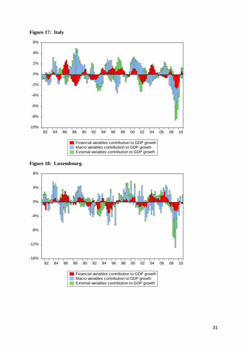
Figure 17: Italy
-10%
-8%
-6%
-4%
-2%
0%
2%
4%
6%
82 84 86 88 90 92 94 96 98 00 02 04 06 08 10
Financial variables contribution to GDP growthMacro variables contribution to GDP growthExternal variables contribution to GDP growth
Figure 18: Luxembourg
-16%
-12%
-8%
-4%
0%
4%
8%
82 84 86 88 90 92 94 96 98 00 02 04 06 08 10
Financial variables contribution to GDP growthMacro variables contribution to GDP growthExternal variables contribution to GDP growth

32
Figure 19: Netherlands
-10%
-8%
-6%
-4%
-2%
0%
2%
4%
82 84 86 88 90 92 94 96 98 00 02 04 06 08 10
Financial variables contribution to GDP growthMacro variables contribution to GDP growthExternal variables contribution to GDP growth
Figure 20: Denmark
-10%
-8%
-6%
-4%
-2%
0%
2%
4%
6%
82 84 86 88 90 92 94 96 98 00 02 04 06 08 10
Financial variables contribution to GDP growthMacro variables contribution to GDP growthExternal variables contribution to GDP growth

33
Figure 21: United Kingdom
-10%
-8%
-6%
-4%
-2%
0%
2%
4%
82 84 86 88 90 92 94 96 98 00 02 04 06 08 10
Financial variables contribution to GDP growthMacro variables contribution to GDP growthExternal variables contribution to GDP growth
Figure 22: Sweden
-12%
-10%
-8%
-6%
-4%
-2%
0%
2%
4%
6%
82 84 86 88 90 92 94 96 98 00 02 04 06 08 10
Financial variables contribution to GDP growthMacro variables contribution to GDP growthExternal variables contribution to GDP growth

34
Figure 23: Australia
-6%
-4%
-2%
0%
2%
4%
6%
82 84 86 88 90 92 94 96 98 00 02 04 06 08 10
Financial variables contribution to GDP growthMacro variables contribution to GDP growthExternal variables contribution to GDP growth
Figure 24: Canada
-8%
-6%
-4%
-2%
0%
2%
4%
6%
84 86 88 90 92 94 96 98 00 02 04 06 08 10
Financial variables contribution to GDP growthMacro variables contribution to GDP growthExternal variables contribution to GDP growth

35
Figure 25: Switzerland
-6%
-4%
-2%
0%
2%
4%
6%
82 84 86 88 90 92 94 96 98 00 02 04 06 08 10
Financial variables contribution to GDP growthMacro variables contribution to GDP growthExternal variables contribution to GDP growth
Figure 26: Japan
-16%
-12%
-8%
-4%
0%
4%
8%
82 84 86 88 90 92 94 96 98 00 02 04 06 08 10
Financial variables contribution to GDP growthMacro variables contribution to GDP growthExternal variables contribution to GDP growth

36
Figure 27: New Zealand
-6%
-4%
-2%
0%
2%
4%
6%
8%
82 84 86 88 90 92 94 96 98 00 02 04 06 08 10
Financial variables contribution to GDP growthMacro variables contribution to GDP growthExternal variables contribution to GDP growth

Paolo Guarda Philippe Jeanfils
Macro-Financial linkages: evidence FroM country-speciFic vars
cahier d’étudesworking paper
n° 71
MarCH 2012
2, boulevard royall-2983 luxembourg
Tél. : +352 4774-1fax: +352 4774 4910
www.bcl.lu • [email protected]