CAFE Scenario Analysis Report Nr. 2 The “Current...

1

CAFE Scenario Analysis Report Nr. 2

The “Current Legislation” and the

“Maximum Technically Feasible Reduction” cases for the

CAFE baseline emission projections

Background paper for the meeting of the

CAFE Working Group on Target Setting and Policy Advice, November 10, 2004

Markus Amann, Rafal Cabala, Janusz Cofala, Chris Heyes, Zbigniew Klimont, Wolfgang Schöpp

International Institute for Applied Systems Analysis (IIASA)

Leonor Tarrason, David Simpson, Peter Wind, Jan-Eiof Jonson Norwegian Meteorological Institute (MET.NO), Oslo, Norway

Version 2 (including tables of impact estimates)

November 2004

International Institute for Applied Systems AnalysisSchlossplatz 1 • A-2361 Laxenburg • Austria

Telephone: (+43 2236) 807 • Fax: (+43 2236) 807 533E-mail: [email protected] • Internet: www.iiasa.ac.at

3

Table of contents

1 INTRODUCTION ......................................................................................................................... 4

2 EMISSION SCENARIOS............................................................................................................. 5

3 ENVIRONMENTAL IMPACTS ............................................................................................... 17

3.1 ANTHROPOGENIC CONTRIBUTIONS TO AMBIENT PM2.5 CONCENTRATIONS........................... 18 3.2 LOSS IN LIFE EXPECTANCY ATTRIBUTABLE TO THE EXPOSURE TO FINE PARTICULATE MATTER

20 3.3 PREMATURE DEATHS ATTRIBUTABLE TO THE EXPOSURE TO GROUND-LEVEL OZONE............. 24 3.4 VEGETATION DAMAGE FROM GROUND-LEVEL OZONE ........................................................... 28 3.5 ACID DEPOSITION TO FOREST ECOSYSTEMS ........................................................................... 30 3.6 ACID DEPOSITION TO SEMI-NATURAL ECOSYSTEMS ............................................................... 34 3.7 ACID DEPOSITION TO FRESHWATER BODIES ........................................................................... 36 3.8 EXCESS NITROGEN DEPOSITION ............................................................................................. 38

International Institute for Applied Systems AnalysisSchlossplatz 1 • A-2361 Laxenburg • Austria

Telephone: (+43 2236) 807 • Fax: (+43 2236) 71313E-mail: [email protected] • Internet: www.iiasa.ac.at

4

1 Introduction The Clean Air For Europe (CAFE) programme of the European Commission aims at a comprehensive assessment of the available measures for further improving European air quality beyond the achievements expected from the full implementation of all present air quality legislation. For this purpose, CAFE has compiled a set of baseline projections outlining the consequences of present legislation on the future development of emissions, of air quality and of health and environmental impacts up to the year 2020.

In its integrated assessment, CAFE will explore the cost-effectiveness of further measures, using the optimization approach of the RAINS model. This optimization will identify the cost-effective set of measures beyond current legislation that achieve exogenously determined environmental policy targets at least costs. For this purpose, the RAINS model will explore in an iterative way the costs and environmental impacts implied by gradually tightened environmental quality objectives, starting from the baseline (current legislation - CLE) case up to the maximum that can be achieved through full application of all presently available technical emission control measures (the maximum feasible reduction case - MFR).

To inform the CAFE Working Group on Target Setting and Policy Advice about the feasible range of targets for environmental improvements between CLE and MFR, this paper presents emissions, resulting air quality and environmental impacts for these two scenarios. The working group is invited to suggest a series of ambition levels of environmental impacts between CLE and MFR, for which the RAINS model will subsequently explore the cost-effective sets of emission control measures that would achieve these targets at least costs.

The paper describes the key results relevant the discussions in the CAFE Working Group on Target Setting and Policy Advice. A comprehensive documentation of the CAFE baseline scenario is provided in Amann et al. (2004). Detailed results on sectoral and country-specific emission estimates can be extracted from the Internet version of the RAINS model (www.iiasa.ac.at/rains).

Section 2 of this report describes the assumptions and results of the emission scenarios. Environmental impacts are presented in Section 3.

This draft paper provides emissions and site-specific impact estimates in form of European maps. Further work will produce summary statistics that present numerical results for all Member States of the European Union. Following the purpose of this paper to assist the Working Group on Target Setting in their deliberations of suitable targets for the RAINS optimization analysis, this provisional report does not address uncertainties in the presented results. The Working Group is invited to advice on the priorities for further work, i.e., of scenario analyses versus uncertainties assessment.

5

2 Emission scenarios This paper explores the feasible ranges of future emissions of air pollutants for

• a “climate policy” scenario, which assumes for the year 2020 a carbon price of 20 €/ton CO2 , achieving a stabilization of the EU-25 CO2 emissions in 2020 compared to 2000 (the “climate policy” CAFE baseline scenario), and

• an “illustrative climate” scenario developed with the PRIMES energy model, assuming a carbon price of 90 €/ton CO2 in 2020. This scenario results in a reduction of the EU-25 CO2 emissions by 20 percent.

For both projections, the RAINS model estimated the air pollutant emissions for

• the “current legislation” (CLE) baseline case, which assumes the implementation of all presently decided emission-related legislation in all countries of the EU-25, and

• the “maximum feasible reduction” (MFR) case, which assumes full implementation of the presently available most advanced technical emission control measures in the year 2020, although excluding premature retirement of existing equipment before the end of its technical life time.

The initial analysis presented in this paper focuses on the year 2020.

Table 2.1: Current legislation and measures assumed for the maximum feasible reduction scenario for SO2 emissions

Legislation considered in the Current Legislation (CLE) scenario Large combustion plant directive Directive on the sulphur content in liquid fuels Directives on quality of petrol and diesel fuels IPPC legislation on process sources National legislation and national practices (if stricter)

Measures assumed for the Maximum Feasible Reduction (MFR) scenario Sector Technology

Power plant boilers - coal, oil and waste fuels High efficiency FGD Power plants, biomass Combustion modification on small biomass boilers Residential/commercial boilers Low sulphur coal and oil Industrial boilers and furnaces FGD on larger boilers, in-furnace controls for

smaller boilers Industrial processes Stage 3 controls Transport (land-based sources) Sulphur-free gasoline and diesel Sea transport Low sulphur marine oils (heavy fuel oil and diesel)

6

Table 2.2: Current legislation and measures assumed for the maximum feasible reduction scenario for NOx emissions

Legislation considered in the Current Legislation (CLE) scenario Large combustion plant directive Auto/Oil EURO standards Emission standards for motorcycles and mopeds Legislation on non-road mobile machinery Implementation failure of EURO-II and Euro-III for heavy duty vehicles IPPC legislation for industrial processes National legislation and national practices (if stricter)


Power plant boilers - coal, oil and gas SCR Power plants, biomass Combustion modification on small biomass boilers,

SCR on large boilers Residential/commercial boilers Combustion modification Industrial boilers and furnaces SCR on larger boilers, SNCR on smaller boilers Industrial processes Stage 3 controls Non-road diesel vehicles (construction, agriculture, inland waterways, railways)

Equivalent to EURO VI on HDVs (post-stage III or IV, depending on a sector and rated power)

Non-road gasoline vehicles (construction, agriculture, inland waterways, railways)

3-way catalytic converters

Motorcycles Stage 3 controls Mopeds Stage 3 controls Heavy-duty trucks - diesel Post-Euro V (Euro VI) Heavy-duty trucks - gasoline Post-Euro V (Euro VI) Light-duty vehicles (gasoline and diesel) Post-EURO IV (Euro VI)

7

Table 2.3: Current legislation and measures assumed for the maximum feasible reduction scenario for VOC emissions

Legislation considered in the Current Legislation (CLE) scenario Stage I directive Directive 91/441 (carbon canisters) Auto/Oil EURO standards Fuel directive (RVP of fuels) Solvents directive Product directive (paints) National legislation, e.g., Stage II


Residential boilers and stoves, coal New boilers or stoves, possibly equipped with oxidation catalysts

Residential stoves and fireplaces, wood Catalytic inserts Extraction and distribution of liquid fuels Vapour balancing on tankers Process emissions in oil refineries Leak detection and repair program and covers on

oil-water separators Evaporative emissions from gasoline vehicles Small carbon canister Gasoline service stations Stage I and II controls Storage and distribution of gasoline Internal floating covers and Stage I controls Dry cleaning New closed circuit machine, hydrocarbon machines

and water-based cleaning Degreasing Closed (sealed) degreaser; use of chlorinated

solvents (or use of A3 solvents and activated carbon filter), water based cleaning

Domestic (personal usage) use of solvents Reformulation of products Decorative paints Simulation of possible developments beyond

Product Directive Vehicle refinishing Primary measures and substitution Wood coating Very high solids systems (5% solvent content)

(additionally small share of low [80% solvents], medium [55%], and high [20%] solid coating systems), application process with an efficiency of 75%

Coil coating Powder coating system (solvent free), thermal oxidation

Automobile production Process modification, substitution, end-of-pipe (adsorption, thermal oxidation)

Leather coating Use of water based coating, bio-filtration Winding wire coating Primary (lower solvent content of enamel and

reduced fugitive emissions) and secondary measures (increased efficiency of the oven)

Other industrial paint use (continuous processes, plastic, general)

Use of current standard solvent based paints (60% solvent content); Use of improved solvent based paints (55%) - application efficiency 65%; Use of water based paints (4-5%) - application efficiency 65 to 98%; Use of powder coatings; application efficiency 90 to 96%

Production of paints, inks and adhesives Upgrade of the condensation units or carbon adsorption and solvent recovery

Printing Low solvent/water based inks and incineration/adsorption (Packaging and Publication); Primary measures, solvent free inks, incineration (Offset); Water based inks, enclosure and incineration (Screen printing)

8

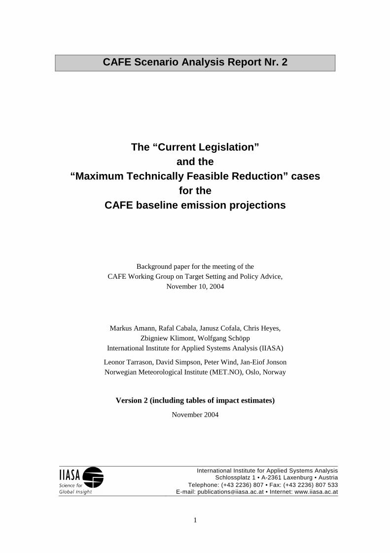
Table 2.4: Current legislation and measures assumed for the maximum feasible reduction scenario for VOC emissions, continued


Industrial glue application Emulsions, hot melts or UV cross-linking acrylates or electron beam curing systems, adsorption, incineration

Wood preservation Use of water based preservatives (conventional application methods) and improved application technique (vacuum impregnation system)

Steam cracking (ethylene and propylene production) and downstream units - chem. ind.

Leak detection and repair program, stage IV

Polystyrene processing 6% pentane expandable beads (85%) and recycled EPS waste (15%) and incineration

PVC production Stripping and vent gas treatment plus optimization of emission treatment including leak and detection program

Pharmaceutical industry Primary measures and high level employment of end-of-pipe measures (incl. thermal incineration, carbon adsorption, condensation, and other)

Storage and handling of chemical products Internal floating covers/sec. seals, vapour recovery (double stage)

Synthetic rubber production Use of 30% solvent based additives and 70% low solvent additives (90% vulcanized rubber and 10% thermoplastic rubber produced) and incineration

Food and drink industry Thermal oxidation Tyre production New process Manufacturing of shoes Good housekeeping and substitution plus automatic

application, biofiltration Fat, edible and non-edible oil extraction Schumacher type desolventiser-toaster-dryer-cooler

plus "a new" hexane recovery section and process optimization

Other industrial sources Good housekeeping in steel industry and switch to emulsion bitumen

Open burning of agricultural and municipal waste

Ban

9

Table 2.5: Current legislation and measures assumed for the maximum feasible reduction scenario for NH3 emissions

Legislation considered in the Current Legislation (CLE) scenario No EU-wide legislation National legislations Current practice


Cattle Low nitrogen feed, housing adaptation, low nitrogen application (specifically distinguishing between options for liquid slurry and solid manure)

Pigs Low nitrogen feed, housing adaptation and closed storage, low nitrogen application (specifically distinguishing between options for liquid slurry and solid manure)

Poultry Low nitrogen feed, housing adaptation and closed storage, bio-filtration, low nitrogen application and incineration of poultry manure (limited number of countries)

Sheep Low nitrogen application N-fertilizer application Substitution of urea with ammonium nitrate Fertilizer production BAT to control end-of-pipe emissions from

fertilizer plants

10

Table 2.6: Current legislation and measures assumed for the maximum feasible reduction scenario for PM2.5 emissions

Legislation considered in the Current Legislation (CLE) scenario Large combustion plant directive Auto/Oil EURO standards for vehicles Emission standards for motorcycles and mopeds Legislation on non-road mobile machinery IPPC legislation on process sources National legislation and national practices (if stricter)


Power plant boilers - coal, oil and gas High efficiency de-dusters (ESP or fabric filters) Power plants, biomass Combustion modification on small biomass boilers Power plants, oil Fabric filters on large boilers, good housekeeping

for smaller boilers Commercial boilers, coal High efficiency de-dusters (cyclons, fabric filters) Residential boilers and stoves, coal New boilers or stoves Residential/commercial boilers (oil) Good housekeeping Residential stoves and fireplaces, wood Catalytic inserts Industrial processes High efficiency de-dusters (ESP or fabric filters),

good practices for fugitive emissions Agriculture Good practices, feed modifications, low till farming

and alternative cereal harvesting Construction Spraying water at construction places Flaring in oil and gas industry Good practices

11

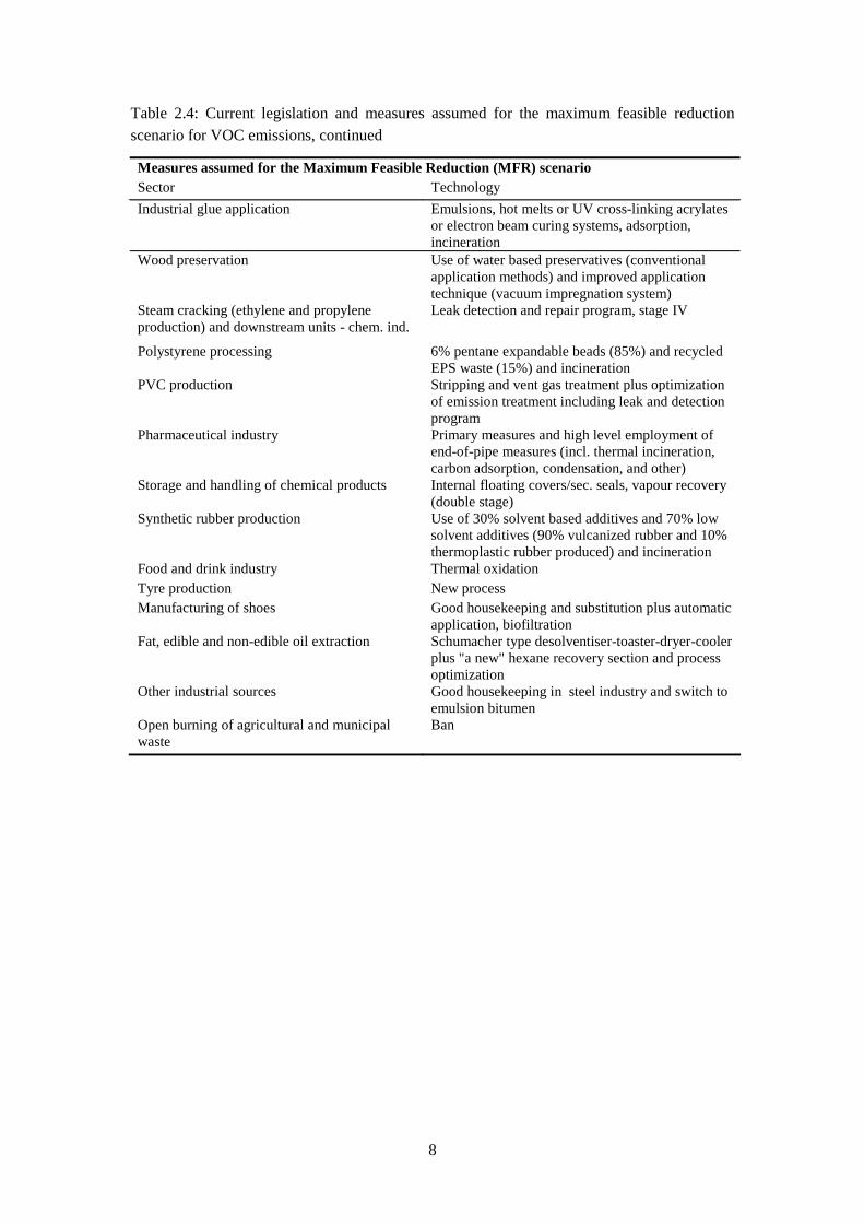
Table 2.7: SO2 emissions for 2000 and 2020, for the "Climate policy" and the "Illustrative climate" scenarios, for current legislation (CLE) and maximum technically feasible reduction (MFR) cases (kt SO2)

2000

“Climate policy” scenario 2020

“Illustrative climate” scenario 2020

CLE MFR CLE MFR

Austria 38 26 22 23 20 Belgium 187 83 51 71 47 Cyprus 46 8 3 7 2 Czech Rep. 250 53 26 36 17 Denmark 28 13 10 13 9 Estonia 91 10 3 7 2 Finland 77 62 46 56 43 France 654 345 148 322 149 Germany 643 332 220 259 177 Greece 481 110 40 100 34 Hungary 487 88 32 77 29 Ireland 132 19 10 18 10 Italy 747 281 117 243 102 Latvia 16 8 2 8 2 Lithuania 43 22 11 19 11 Luxembourg 4 2 1 2 1 Malta 26 2 1 1 1 Netherlands 84 64 41 62 40 Poland 1515 554 223 385 178 Portugal 230 81 33 74 30 Slovakia 124 33 13 25 9 Slovenia 97 16 8 14 7 Spain 1489 335 155 315 153 Sweden 58 50 39 49 38 UK 1186 209 102 202 100 EU-25 8735 2805 1357 2387 1211 Atlantic Ocean 397 657 146 657 146 Baltic Sea 243 225 90 225 90 Black Sea 84 138 31 138 31 Mediterranean 1244 2082 464 2082 464 North Sea 461 424 169 424 169 Sea regions 2430 3526 900 3526 900

12

Table 2.8: NOx emissions for 2000 and 2020, for the "Climate policy" and the "Illustrative climate" scenarios, for current legislation (CLE) and maximum technically feasible reduction (MFR) cases (kt NOx)

2000



CLE MFR CLE MFR


13

Table 2.9: VOC emissions for 2000 and 2020, for the "Climate policy" and the "Illustrative climate" scenarios, for current legislation (CLE) and maximum technically feasible reduction (MFR) cases (kt VOC)

2000



CLE MFR CLE MFR


14

Table 2.10: NH3 emissions for 2000 and 2020, for the "Climate policy" and the "Illustrative climate" scenarios, for current legislation (CLE) and maximum technically feasible reduction (MFR) cases (kt NH3)

2000



CLE MFR CLE MFR

Austria 54 54 27 54 27 Belgium 81 76 47 76 47 Cyprus 6 6 3 6 3 Czech Rep. 74 65 36 65 36 Denmark 91 78 40 78 40 Estonia 10 12 5 12 5 Finland 35 32 22 32 22 France 728 702 387 702 386 Germany 638 603 441 599 437 Greece 55 52 34 51 34 Hungary 78 85 39 85 39 Ireland 127 121 84 121 83 Italy 432 399 248 398 246 Latvia 12 16 7 16 7 Lithuania 50 57 39 57 39 Luxembourg 7 6 4 6 4 Malta 1 1 1 1 1 Netherlands 157 140 103 139 103 Poland 309 333 150 332 147 Portugal 68 67 40 67 39 Slovakia 32 33 17 32 16 Slovenia 18 20 9 20 9 Spain 394 370 197 370 197 Sweden 53 49 33 48 33 UK 315 310 206 310 203 EU-25 3824 3686 2221 3679 2203

15

Table 2.11: Primary PM2.5 emissions for 2000 and 2020, for the "Climate policy" and the "Illustrative climate" scenarios, for current legislation (CLE) and maximum technically feasible reduction (MFR) cases (kt PM2.5)

2000



CLE MFR CLE MFR


16

0%

50%

100%

150%

200%

250%

300%

1990 1995 2000 2005 2010 2015 2020 2025 2030

SO2 NOx VOC NH3 PM2.5

Figure 2.1: Long-term trends in EU-25 emissions relative to the year 2000

0%

20%

40%

60%

80%

100%

SO2 NOx VOC NH3 PM2.5

2000 Current legislation 2020 Maximum feasible reductions 2020

Figure 2.2: Scope for further technical emission control measures in 2020 in the EU-25 (2000 = 100%)

17

3 Environmental impacts For the purpose of exploring the cost-effectiveness of further emission control measures, this paper analyses the impacts of the emission reductions outlined in the preceding sections on a range of health and environmental endpoints.

While inter-annual meteorological variability is an important aspect that must be considered in the design of cost-effective air quality management strategies, the provisional analysis presented in this paper is carried out for the meteorological conditions of a single year (1997). This simplification is caused by the high computational demand of developing atmospheric source-receptor relationships, which form one backbone in the RAINS optimization approach. Due to constraints in computer time, up to now source-receptor relationships could only be developed for one meteorological year. The assessment of the CAFE baseline scenario has considered the meteorological conditions of four years (1997, 1999, 2000 and 2003), finding that at least for particulate matter 1997 did not represent extreme conditions. Thus, to provide a background for setting environmental targets for the first round of the RAINS optimization analyses, this paper evaluates the environmental impacts in a way that is fully compatible with the (provisional) RAINS optimization framework, i.e., for 1997. Eventually, when refining the assessment, the inter-annual meteorological variability has to be taken into account.

With decreasing emissions from European sources, European air quality is increasingly influenced by hemispheric background pollution. The atmospheric computations of the EMEP model conducted for the CAFE analysis consider present background levels as boundary conditions to their calculations. For ozone, however, a wide range of scientific literature hints at increasing background concentrations resulting from intercontinental and hemispheric transport, essentially caused by global increases in methane emissions and steep growth in Asian emissions of NOx and VOC. Thus, any considerations of future environmental air quality targets for Europe should not forget the ongoing increases in background pollution, in order to set European emission control efforts into a realistic context. For this purpose, the analysis presented in this paper assumes for the year 2020 a 3 ppb increase in hemispheric background levels of ozone compared to the year 2000.

As an initial analysis, this paper presents the environmental impacts for the “Climate policy” scenario. Due to time constraints it was not possible to finalize the impacts assessment for the “Illustrative climate” scenario before the meeting of the Working Group on Target Setting and Policy Advice. However, the emission estimates listed in the preceding section for the “Illustrative climate” scenario provide some indication of the additional scope for air quality improvements resulting from more aggressive greenhouse gas control strategies.

18

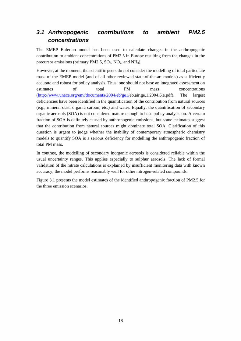
3.1 Anthropogenic contributions to ambient PM2.5 concentrations

The EMEP Eulerian model has been used to calculate changes in the anthropogenic contribution to ambient concentrations of PM2.5 in Europe resulting from the changes in the precursor emissions (primary PM2.5, SO2, NOx, and NH3).

However, at the moment, the scientific peers do not consider the modelling of total particulate mass of the EMEP model (and of all other reviewed state-of-the-art models) as sufficiently accurate and robust for policy analysis. Thus, one should not base an integrated assessment on estimates of total PM mass concentrations (http://www.unece.org/env/documents/2004/eb/ge1/eb.air.ge.1.2004.6.e.pdf). The largest deficiencies have been identified in the quantification of the contribution from natural sources (e.g., mineral dust, organic carbon, etc.) and water. Equally, the quantification of secondary organic aerosols (SOA) is not considered mature enough to base policy analysis on. A certain fraction of SOA is definitely caused by anthropogenic emissions, but some estimates suggest that the contribution from natural sources might dominate total SOA. Clarification of this question is urgent to judge whether the inability of contemporary atmospheric chemistry models to quantify SOA is a serious deficiency for modelling the anthropogenic fraction of total PM mass.

In contrast, the modelling of secondary inorganic aerosols is considered reliable within the usual uncertainty ranges. This applies especially to sulphur aerosols. The lack of formal validation of the nitrate calculations is explained by insufficient monitoring data with known accuracy; the model performs reasonably well for other nitrogen-related compounds.

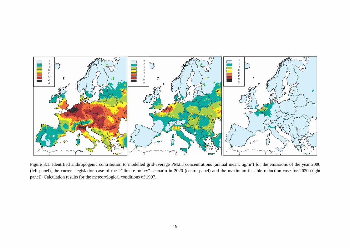
Figure 3.1 presents the model estimates of the identified anthropogenic fraction of PM2.5 for the three emission scenarios.

19

Figure 3.1: Identified anthropogenic contribution to modelled grid-average PM2.5 concentrations (annual mean, µg/m3) for the emissions of the year 2000 (left panel), the current legislation case of the “Climate policy” scenario in 2020 (centre panel) and the maximum feasible reduction case for 2020 (right panel). Calculation results for the meteorological conditions of 1997.

20

3.2 Loss in life expectancy attributable to the exposure to fine particulate matter

With the methodology described in Amann et al. (2004), the RAINS model estimates changes in the loss in statistical life expectancy that can be attributed to changes in anthropogenic emissions (ignoring the role of secondary organic aerosols). This calculation is based on the assumption that health impacts can be associated with changes in PM2.5 concentrations. Following the advice of the joint World Health Organization/UNECE Task Force on Health (http://www.unece.org/env/documents/2004/eb/wg1/eb.air.wg1.2004.11.e.pdf), RAINS applies a linear concentration-response function and associates all changes in the identified anthropogenic fraction of PM2.5 with health impacts. Thereby, no health impacts are calculated for PM from natural sources and for secondary organic aerosols. It transfers the rate of relative risk for PM2.5 identified by Pope et al. (2002) for 500.000 individuals in the United States to the European situation and calculates mortality for the population older than 30 years. Thus, the assessment in RAINS does not quantify infant mortality and thus underestimates overall effects. Awaiting results from the City-Delta project, the provisional estimates presented in this report assume PM2.5 concentrations originating from primary emissions in urban areas to be 25 percent higher than in the surrounding rural areas.

21

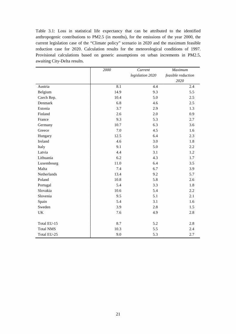
Table 3.1: Loss in statistical life expectancy that can be attributed to the identified anthropogenic contributions to PM2.5 (in months), for the emissions of the year 2000, the current legislation case of the “Climate policy” scenario in 2020 and the maximum feasible reduction case for 2020. Calculation results for the meteorological conditions of 1997. Provisional calculations based on generic assumptions on urban increments in PM2.5, awaiting City-Delta results.

2000 Current

legislation 2020

Maximum

feasible reduction

2020

Austria 8.1 4.4 2.4

Belgium 14.9 9.3 5.5 Czech Rep. 10.4 5.0 2.5 Denmark 6.8 4.6 2.5 Estonia 3.7 2.9 1.3 Finland 2.6 2.0 0.9 France 9.3 5.3 2.7 Germany 10.7 6.3 3.6 Greece 7.0 4.5 1.6 Hungary 12.5 6.4 2.3 Ireland 4.6 3.0 1.8 Italy 9.1 5.0 2.2 Latvia 4.4 3.1 1.2 Lithuania 6.2 4.3 1.7 Luxembourg 11.0 6.4 3.5 Malta 7.4 6.7 3.9 Netherlands 13.4 9.2 5.7 Poland 10.8 5.8 2.6 Portugal 5.4 3.3 1.8 Slovakia 10.6 5.4 2.2 Slovenia 9.5 5.1 2.1 Spain 5.4 3.1 1.6 Sweden 3.9 2.8 1.5 UK 7.6 4.9 2.8 Total EU-15 8.7 5.2 2.8 Total NMS 10.3 5.5 2.4 Total EU-25 9.0 5.3 2.7

22

0

2

4

6

8

10

12

14

16

Aus

tria

Bel

gium

Cze

ch R

ep.

Den

mar

k

Est

onia

Fin

land

Fra

nce

Ger

man

y

Gre

ece

Hun

gary

Irel

and

Italy

Latv

ia

Lith

uani

a

Luxe

mbo

urg

Mal

ta

Net

herla

nds

Pol

and

Por

tuga

l

Slo

vaki

a

Slo

veni

a

Spa

in

Sw

eden UK

Tot

al E

U-1

5

Tot

al N

MS

Tot

al E

U-2

5

2000 CLE 2020 MFR 2020

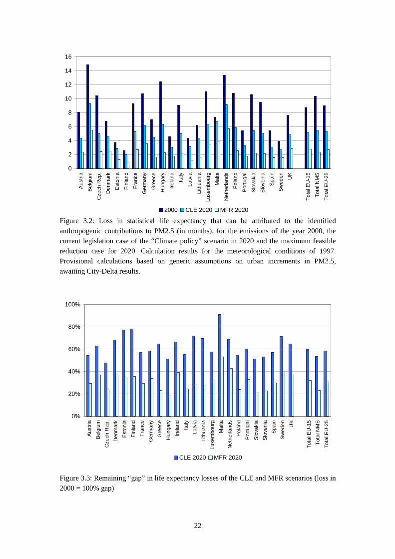
Figure 3.2: Loss in statistical life expectancy that can be attributed to the identified anthropogenic contributions to PM2.5 (in months), for the emissions of the year 2000, the current legislation case of the “Climate policy” scenario in 2020 and the maximum feasible reduction case for 2020. Calculation results for the meteorological conditions of 1997. Provisional calculations based on generic assumptions on urban increments in PM2.5, awaiting City-Delta results.

0%

20%

40%

60%

80%

100%

Aus

tria

Bel

gium

Cze

ch R

ep.

Den

mar

k

Est

onia

Fin

land

Fra

nce

Ger

man

y

Gre

ece

Hun

gary

Irel

and

Italy

Latv

ia

Lith

uani

a

Luxe

mbo

urg

Mal

ta

Net

herla

nds

Pol

and

Por

tuga

l

Slo

vaki

a

Slo

veni

a

Spa

in

Sw

eden UK

Tot

al E

U-1

5

Tot

al N

MS

Tot

al E

U-2

5

CLE 2020 MFR 2020

Figure 3.3: Remaining “gap” in life expectancy losses of the CLE and MFR scenarios (loss in 2000 = 100% gap)

23

Figure 3.4: Loss in statistical life expectancy that can be attributed to the identified anthropogenic contributions to PM2.5 (in months), for the emissions of the year 2000 (left panel), the current legislation case of the “Climate policy” scenario in 2020 (centre panel) and the maximum feasible reduction case for 2020 (right panel). Calculation results for the meteorological conditions of 1997. Provisional calculations based on generic assumptions on urban increments in PM2.5, awaiting City-Delta results.

24

3.3 Premature deaths attributable to the exposure to ground-level ozone

The joint WHO/UNECE Task Force at its 7th Meeting developed specific recommendations concerning the inclusion of ozone-related mortality into RAINS. Key points of these recommendations are summarised below:

• The relevant health endpoint is mortality, even though several effects of ozone on morbidity are also well documented and causality established; however, available input data (e.g., on base rates) to calculate the latter on a European scale are often either lacking or not comparable.

• The relative risk for all-cause mortality is taken from the recent meta-analysis of European time-series studies, which was commissioned by WHO and performed by a group of experts of St. George’s Hospital in London, UK (WHO, 2004). The relative risk taken from this study is 1.003 for a 10 µg/m3 increase in the daily maximum 8-hour mean (CI 1.001 and 1.004).

• In agreement with the recent findings of the WHO Systematic Review, a linear concentration-response function is applied.

• The effects of ozone on mortality are calculated from the daily maximum 8-hour mean. This is in line with the health studies used to derive the summary estimate used for the meta-analysis mentioned above.

• Even though current evidence was insufficient to derive a level below which ozone has no effect on mortality, a cut-off at 35 ppb, considered as a daily maximum 8-hour mean ozone concentration, is used. This means that for days with ozone concentration above 35 ppb as maximum 8-hour mean, only the increment exceeding 35 ppb is used to calculate effects. No effects of ozone on health are calculated on days below 35 ppb as maximum 8-hour mean. This exposure parameter is called SOMO35 (sum of means over 35) and is the sum of excess of daily maximum 8-h means over the cut-off of 35 ppb calculated for all days in a year. This is illustrated in the following figure.

The Eulerian EMEP model has been used to calculate the SOMO35 exposure indicator referred to above for the baseline emission projections. RAINS applies the SOMO35 based methodology to quantify the changes in premature mortality that are attributable to the projected reductions in ozone precursor emissions. However, these estimates are loaded with considerable uncertainties of different types, and further analysis is necessary to explore the robustness of these figures. In particular, these numbers are derived from time series studies assessing the impacts of daily changes in ozone levels on daily mortality rates. By their nature, such studies cannot provide any indication on how much the deaths have been brought forward, and some of these deaths are considered as “harvesting effects” followed by reduced mortality few days later. At present it is not possible to quantify the importance of this effect for these estimates. Also the influence of the selected cut-off value (35 ppb) on the outcome needs to be further explored in the future.

25

Figure 3.5: Grid-average ozone concentrations expressed as SOMO35 for the year 2000 (left panel), the current legislation case of the “Climate policy” scenario in 2020 (centre panel) and the maximum feasible reduction case for 2020 (right panel), in ppb.days. Calculation results for the meteorological conditions of 1997.

26

Table 3.2: Provisional estimates of premature mortality attributable to ozone for the “no further climate measures” CAFE baseline scenario (cases of premature deaths per year). These calculations are based on regional scale ozone calculations (50*50 km) and apply the meteorological conditions of 1997. No estimates have been performed for Cyprus and Malta.

2000 CLE 2020 MFR 2020

Austria 422 316 220 Belgium 381 340 309 Denmark 179 160 126 Finland 58 60 39 France 2663 2180 1655 Germany 4258 3306 2535 Greece 627 567 334 Ireland 74 80 68 Italy 4507 3581 2583 Luxembourg 31 26 20 Netherlands 416 362 336 Portugal 450 443 350 Spain 2002 1705 1271 Sweden 197 189 135 UK 1423 1698 1554 Total EU-15 18110 15307 11711 Czech Rep. 535 390 257 Estonia 21 22 13 Hungary 748 574 300 Latvia 65 66 35 Lithuania 66 65 29 Poland 1399 1117 609 Slovakia 239 177 99 Slovenia 112 82 52 Total NMS 3215 2516 1418 Total 21429 17938 13288

27

0

1000

2000

3000

4000

5000

Aus

tria

Bel

gium

Den

mar

k

Fin

land

Fra

nce

Ger

man

y

Gre

ece

Irel

and

Italy

Luxe

mbo

urg

Net

herla

nds

Por

tuga

l

Spa

in

Sw

eden UK

Cze

ch R

ep.

Est

onia

Hun

gary

Latv

ia

Lith

uani

a

Pol

and

Slo

vaki

a

Slo

veni

a

2000 CLE 2020 MFR 2020

Figure 3.6: Provisional estimates of premature mortality attributable to ozone for the “no further climate measures” CAFE baseline scenario (cases of premature deaths per year). These calculations are based on regional scale ozone calculations (50*50 km) and apply the meteorological conditions of 1997. No estimates have been performed for Cyprus and Malta.

0%

20%

40%

60%

80%

100%

120%

Aus

tria

Bel

gium

Den

mar

k

Fin

land

Fra

nce

Ger

man

y

Gre

ece

Irel

and

Italy

Luxe

mbo

urg

Net

herla

nds

Por

tuga

l

Spa

in

Sw

eden UK

Cze

ch R

ep.

Est

onia

Hun

gary

Latv

ia

Lith

uani

a

Pol

and

Slo

vaki

a

Slo

veni

a

CLE 2020 MFR 2020

Figure 3.7: Remaining “gaps” in premature deaths attributable to ozone of the CLE and MFR scenarios (loss in 2000 = 100% gap)

28

3.4 Vegetation damage from ground-level ozone

The RAINS model applies the concept of critical levels to quantify progress towards the environmental long-term target of full protection of vegetation from ozone damage. At the UNECE workshop in Gothenburg in November 2002 (Karlsson et al., 2003) it was concluded that the effective ozone dose, based on the flux of ozone into the leaves through the stomatal pores, represents the most appropriate approach for setting future ozone critical levels for forest trees. However, uncertainties in the development and application of flux-based approaches to setting critical levels for forest trees are at present too large to justify their application as a standard risk assessment method at a European scale.

Consequently, the UNECE Working Group on Effects retains in its Mapping Manual the AOT40 (accumulated ozone over a threshold of 40 ppb) approach as the recommended method for integrated risk assessment for forest trees, until the ozone flux approach will be sufficiently refined. However, such AOT40 measures are not considered suitable for quantifying vegetation damage, but can only be used as indicators for quantifying progress towards the environmental long-term targets.

The Mapping Manual defines critical levels for crops, forests and semi-natural vegetation in terms of different levels of AOT40, measured over different time spans. From earlier analysis of ozone time series for various parts of Europe, the critical level for forest trees (5 ppm.hours over the full vegetation period, April 1- September 30 is recommended as default) appears as the most stringent constraint. For most parts of Europe, the other critical levels will be automatically achieved if the 5 ppm.hours over six months condition is satisfied. Thus, if used for setting environmental targets for emission reduction strategies, the critical levels for forest trees would imply protection of the other receptors.

Figure 3.8 presents the evolution of the excess ozone that is considered harmful for forest trees, using the AOT40 (accumulated ozone over a threshold of 40 ppb) as a metric. The updated manual for critical levels (UNECE, 2004) specifies a no-effect critical level of 5 ppm.hours for trees. Related to this quantity, significant excess ozone is calculated for 2000 for large parts of the European Union. Baseline emission reductions will improve the situation, but will not be sufficient to eliminate the risk even by 2020.

29

Figure 3.8: AOT40 for the year 2000 (left panel), the current legislation case of the “Climate policy” scenario in 2020 (centre panel) and the maximum feasible reduction case for 2020 (right panel), in ppm.hours. Calculation results for the meteorological conditions of 1997. The critical level for forests is set at 5 ppm.hours.

30

3.5 Acid deposition to forest ecosystems

RAINS used the concept of critical loads as a quantitative indicator for sustainable levels of sulphur and nitrogen deposition. The analysis using is based on the critical loads databases compiled by the Coordination Centre on Effects under the UNECE Working Group on Effects. This database combines quality-controlled critical loads estimates of the national focal centres for more than 1.6 million ecosystems (Posch et al., 2004). National focal centres have selected a variety of ecosystem types as receptors for calculating and mapping critical loads. For most ecosystem types (e.g., forests), critical loads are calculated for both acidity and eutrophication. Other receptor types, such as streams and lakes, have only critical loads for acidity, on the assumption that eutrophication does not occur in these ecosystems. The RAINS analysis groups ecosystems into three classes (forests, semi-natural vegetation such as nature protection areas and freshwater bodies) and performs separate analyses for each class. The RAINS analysis compares for a given emission scenario the resulting deposition to these ecosystems with the critical loads and thus provides an indication to what extent the various types of ecosystems are still at risk of acidification. This indicator cannot be directly interpreted as the actual damage occurring at such ecosystems. To derive damage estimates, the historic rate of acid deposition as well as dynamic chemical processes in soils and lakes need to be considered, which can lead to substantial delays in the occurrence of acidification as well as in the recovery from acidification.

31

Table 3.3: Percentage of forest area receiving acid deposition above the critical loads for the baseline emissions for 2000, the current legislation case of the “Climate policy” scenario in 2020 and the maximum feasible reduction case for 2020. Calculation results for the meteorological conditions of 1997, using ecosystem-specific deposition for forests. Critical loads data base of 2004.

2000 CLE MFR

Austria 15.2 5.0 0.5

Belgium 55.4 31.6 13.3 Denmark 31.8 8.5 0.3 Finland 1.6 1.5 0.4 France 12.4 4.8 0.7 Germany 72.3 41.6 12.9 Greece 0.6 0.0 0.0 Ireland 47.0 19.2 9.1 Italy 2.3 1.0 0.3 Luxembourg 35.1 11.6 0.0 Netherlands 88.3 80.4 52.3 Portugal 2.6 0.2 0.0 Spain 1.0 0.0 0.0 Sweden 23.7 18.7 8.4 UK 49.0 17.6 6.0 Total EU-15 17.7 10.5 3.7 Czech Rep. 80.8 42.0 1.8 Estonia 0.3 0.0 0.0 Hungary 3.9 1.5 0.0 Latvia 0.6 0.5 0.0 Lithuania 2.9 1.0 0.0 Poland 59.0 21.8 0.2 Slovakia 22.7 7.7 0.4 Slovenia 2.8 0.1 0.0 Total NMS 35.7 14.2 0.3 Total EU-25 20.8 11.1 3.1

32

0%

20%

40%

60%

80%

100%

Aus

tria

Bel

gium

Den

mar

k

Fin

land

Fra

nce

Ger

man

y

Gre

ece

Irel

and

Italy

Luxe

mbo

urg

Net

herla

nds

Por

tuga

l

Spa

in

Sw

eden UK

Tot

al E

U-1

5

Cze

ch R

ep.

Est

onia

Hun

gary

Latv

ia

Lith

uani

a

Pol

and

Slo

vaki

a

Slo

veni

a

Tot

al N

MS

Tot

al E

U-2

5

2000 CLE MFR

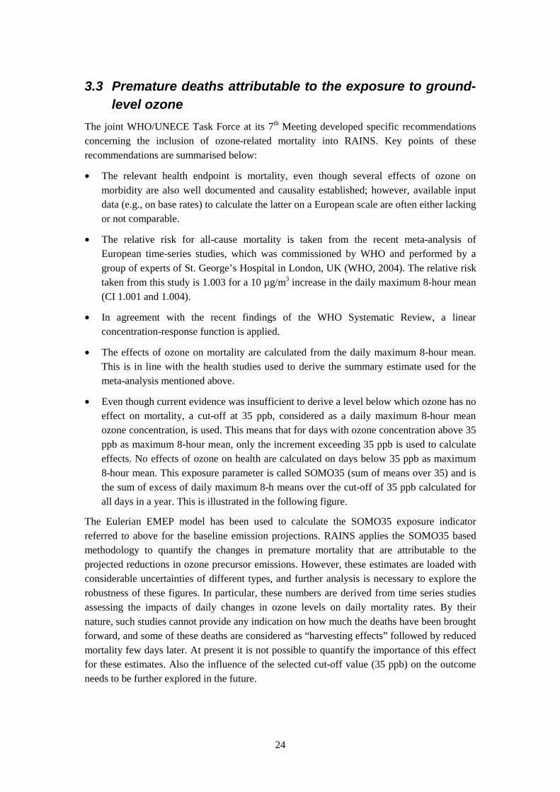
Figure 3.9: Percentage of forest area receiving acid deposition above the critical loads for the baseline emissions for 2000, the current legislation case of the “Climate policy” scenario in 2020 and the maximum feasible reduction case for 2020. Calculation results for the meteorological conditions of 1997, using ecosystem-specific deposition for forests. Critical loads data base of 2004.

0%

20%

40%

60%

80%

100%

Aus

tria

Bel

gium

Den

mar

k

Fin

land

Fra

nce

Ger

man

y

Gre

ece

Irel

and

Italy

Luxe

mbo

urg

Net

herla

nds

Por

tuga

l

Spa

in

Sw

eden UK

Tot

al E

U-1

5

Cze

ch R

ep.

Est

onia

Hun

gary

Latv

ia

Lith

uani

a

Pol

and

Slo

vaki

a

Slo

veni

a

Tot

al N

MS

Tot

al E

U-2

5

CLE MFR

Figure 3.10: Remaining “gaps” in unprotected forest ecosystems of the CLE and MFR scenario related to the situation in 2000 (2000 = 100% gap)

33

Figure 3.11: Percentage of forest area receiving acid deposition above the critical loads for the baseline emissions for 2000 (left panel), the current legislation case of the “Climate policy” scenario in 2020 (centre panel) and the maximum feasible reduction case for 2020 (right panel). Calculation results for the meteorological conditions of 1997, using ecosystem-specific deposition for forests. Critical loads data base of 2004.

34

3.6 Acid deposition to semi-natural ecosystems

A number of countries have provided estimates of critical loads for so-called “semi-natural” ecosystems. This group typically contains nature and landscape protection areas, many of them designated as “Natura2000” areas of the EU Habitat directive. While this group of ecosystems includes open land and forest areas, RAINS uses as a conservative estimate grid-average deposition rates for the comparison with critical loads, which systematically underestimates deposition for forested land.

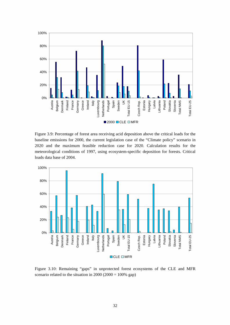
Table 3.4: Area with semi-natural ecosystems with acid deposition above critical loads (in km2) for the “no further climate measures” scenario. The analysis reflects average meteorological conditions of 1997

Percent of semi-natural ecosystems area

Semi-natural ecosystems area with acid deposition above critical loads

2000 CLE 2020 MFR 2020 2000 CLE 2010 MFR 2020 France 37.6 9.0 0.6 376032 90328 6008 Germany 68.1 40.9 11.3 268750 161487 44752 Ireland 10.3 2.3 0.4 47429 10786 1982 Italy 0.0 0.0 0.0 261 0 0 Netherlands 63.0 47.8 17.8 81711 61970 23111 UK 30.8 9.3 1.3 1528760 459721 65106

Total 24.1 8.2 1.5 2302941 784291 140960

0

10

20

30

40

50

60

70

France Germany Ireland Italy Netherlands UK Total

2000 CLE 2020 MFR 2020

Figure 3.12: Percentage of the area of semi-natural ecosystems receiving acid deposition above the critical loads, for the baseline emissions for 2000, the CLE case in 2020 and the MFR case for 2020. Calculation results for the meteorological conditions of 1997, using grid-average deposition.

35

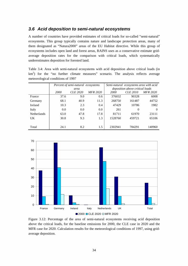
Figure 3.13: Percentage of the area of semi-natural ecosystems receiving acid deposition above the critical loads, for the baseline emissions for 2000 (left panel), the current legislation case of the “Climate policy” scenario in 2020 (centre panel) and the maximum feasible reduction case for 2020 (right panel). Calculation results for the meteorological conditions of 1997, using grid-average deposition. Critical loads data base of 2004. For areas shown in white no critical loads estimates have been provided.

36

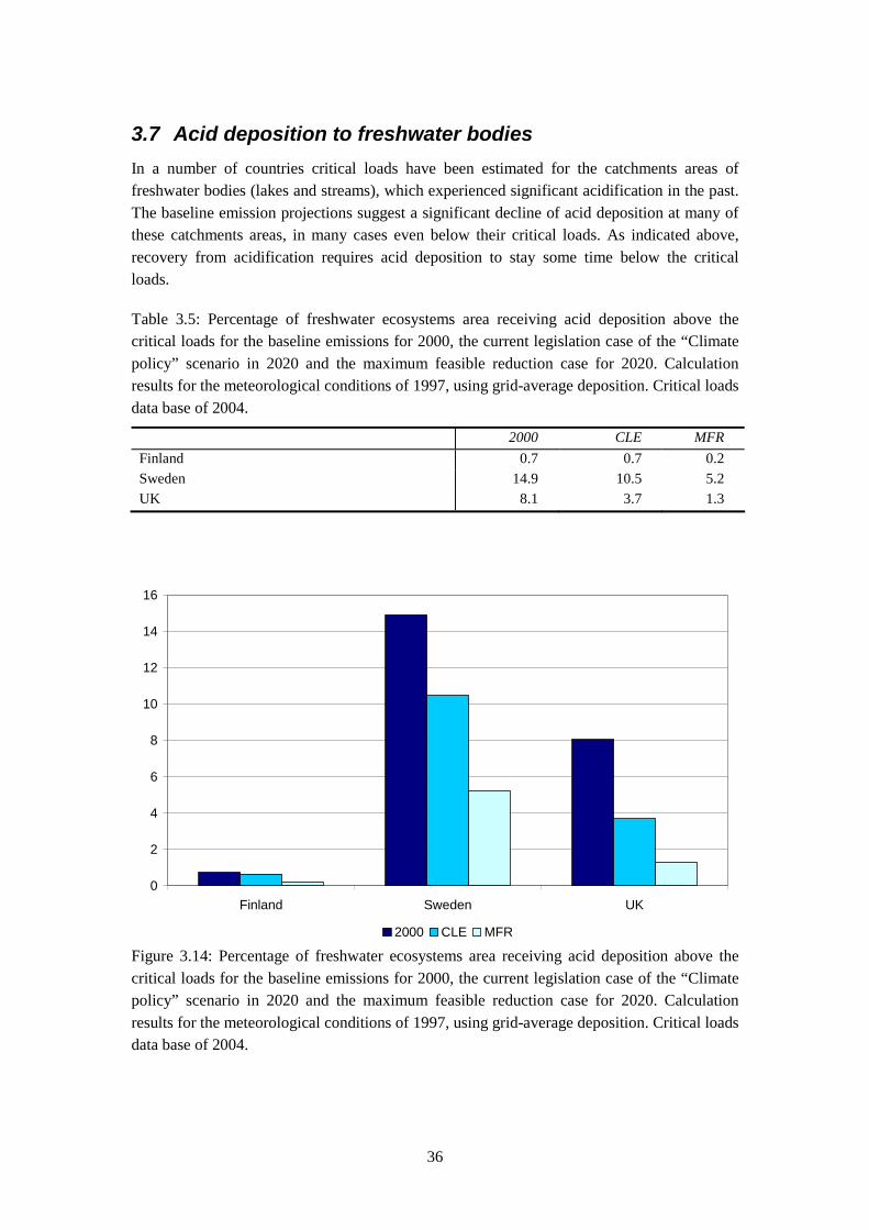
3.7 Acid deposition to freshwater bodies

In a number of countries critical loads have been estimated for the catchments areas of freshwater bodies (lakes and streams), which experienced significant acidification in the past. The baseline emission projections suggest a significant decline of acid deposition at many of these catchments areas, in many cases even below their critical loads. As indicated above, recovery from acidification requires acid deposition to stay some time below the critical loads.

Table 3.5: Percentage of freshwater ecosystems area receiving acid deposition above the critical loads for the baseline emissions for 2000, the current legislation case of the “Climate policy” scenario in 2020 and the maximum feasible reduction case for 2020. Calculation results for the meteorological conditions of 1997, using grid-average deposition. Critical loads data base of 2004.

2000 CLE MFR

Finland 0.7 0.7 0.2 Sweden 14.9 10.5 5.2 UK 8.1 3.7 1.3

0

2

4

6

8

10

12

14

16

Finland Sweden UK

2000 CLE MFR

Figure 3.14: Percentage of freshwater ecosystems area receiving acid deposition above the critical loads for the baseline emissions for 2000, the current legislation case of the “Climate policy” scenario in 2020 and the maximum feasible reduction case for 2020. Calculation results for the meteorological conditions of 1997, using grid-average deposition. Critical loads data base of 2004.

37

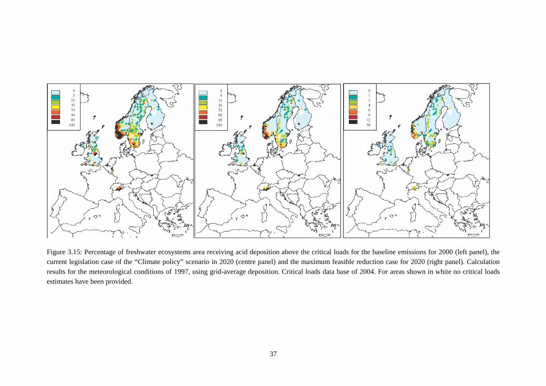
Figure 3.15: Percentage of freshwater ecosystems area receiving acid deposition above the critical loads for the baseline emissions for 2000 (left panel), the current legislation case of the “Climate policy” scenario in 2020 (centre panel) and the maximum feasible reduction case for 2020 (right panel). Calculation results for the meteorological conditions of 1997, using grid-average deposition. Critical loads data base of 2004. For areas shown in white no critical loads estimates have been provided.

38

3.8 Excess nitrogen deposition

Excess nitrogen deposition poses a threat to a wide range of ecosystems endangering their bio-diversities through changes in the plant communities. Critical loads indicating the maximum level of nitrogen deposition that can be absorbed by ecosystems without eutrophication have been estimated throughout Europe. As a conservative estimate, the assessment presented in this report uses grid-average deposition for all ecosystems, resulting in a systematic underestimate of nitrogen deposition to forests.

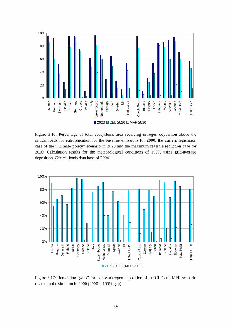
Table 3.6: Percentage of total ecosystems area receiving nitrogen deposition above the critical loads for eutrophication for the baseline emissions for 2000, the current legislation case of the “Climate policy” scenario in 2020 and the maximum feasible reduction case for 2020. Calculation results for the meteorological conditions of 1997, using grid-average deposition. Critical loads data base of 2004.

2020 CLE 2020 MFR 2020

Austria 96.0 86.4 52.9 Belgium 92.7 60.8 23.3 Denmark 52.7 37.2 0.8 Finland 25.1 14.4 0.0 France 95.8 79.1 20.2 Germany 96.2 94.4 85.5 Greece 75.8 72.9 2.0 Ireland 11.6 3.3 0.0 Italy 62.3 47.7 12.8 Luxembourg 96.4 82.1 39.6 Netherlands 66.5 60.8 26.7 Portugal 29.7 12.0 0.0 Spain 64.6 50.1 6.7 Sweden 26.1 16.1 0.6 UK 13.3 5.5 0.0 Total EU-15 54.3 43.0 16.0 Czech Rep. 95.2 76.6 11.9 Estonia 11.7 5.8 0.0 Hungary 30.7 24.4 4.6 Latvia 54.3 38.0 0.5 Lithuania 85.0 80.8 4.4 Poland 86.0 78.8 17.8 Slovakia 88.8 60.2 4.4 Slovenia 94.3 88.0 20.8 Total NMS 71.2 60.3 10.1 Total EU-25 57.1 45.9 15.1

39

0

20

40

60

80

100

Aus

tria

Bel

gium

Den

mar

k

Fin

land

Fra

nce

Ger

man

y

Gre

ece

Irel

and

Italy

Luxe

mbo

urg

Net

herla

nds

Por

tuga

l

Spa

in

Sw

eden UK

Tot

al E

U-1

5

Cze

ch R

ep.

Est

onia

Hun

gary

Latv

ia

Lith

uani

a

Pol

and

Slo

vaki

a

Slo

veni

a

Tot

al N

MS

Tot

al E

U-2

5

2020 CEL 2020 MFR 2020

Figure 3.16: Percentage of total ecosystems area receiving nitrogen deposition above the critical loads for eutrophication for the baseline emissions for 2000, the current legislation case of the “Climate policy” scenario in 2020 and the maximum feasible reduction case for 2020. Calculation results for the meteorological conditions of 1997, using grid-average deposition. Critical loads data base of 2004.

0%

20%

40%

60%

80%

100%

Aus

tria

Bel

gium

Den

mar

k

Fin

land

Fra

nce

Ger

man

y

Gre

ece

Irel

and

Italy

Luxe

mbo

urg

Net

herla

nds

Por

tuga

l

Spa

in

Sw

eden UK

Tot

al E

U-1

5

Cze

ch R

ep.

Est

onia

Hun

gary

Latv

ia

Lith

uani

a

Pol

and

Slo

vaki

a

Slo

veni

a

Tot

al N

MS

Tot

al E

U-2

5

CLE 2020 MFR 2020

Figure 3.17: Remaining “gaps” for excess nitrogen deposition of the CLE and MFR scenario related to the situation in 2000 (2000 = 100% gap)

40

Figure 3.18: Percentage of total ecosystems area receiving nitrogen deposition above the critical loads for eutrophication for the baseline emissions for 2000 (left panel), the current legislation case of the “Climate policy” scenario in 2020 (centre panel) and the maximum feasible reduction case for 2020 (right panel). Calculation results for the meteorological conditions of 1997, using grid-average deposition. Critical loads data base of 2004. For areas shown in white no critical loads estimates have been provided.

41

References

Amann, M., Bertok, I., Cofala, J., Gyarfas, F., Heyes, C., Klimont, Z., Schöpp, W. and Winiwarter, W. (2004) Baseline Scenarios for the Clean Air for Europe (CAFE) Programme. International Institute for Applied Systems Analysis (IIASA), Laxenburg, Austria.

Amann, M., Cofala, J., Heyes, C., Klimont, Z., Mechler, R., Posch, M. and Schoepp, W. (2004) The RAINS model. Documentation of the model approach prepared for the RAINS review. International Institute for Applied Systems Analysis (IIASA), Laxenburg, Austria (http://www.iiasa.ac.at/rains/review/review-full.pdf)

Karlsson, P. E., Selldén, G. and Pleijel, H. (2003) Establishing Ozone Critical Levels II. UNECE Workshop Report. IVL report B 1523., IVL Swedish Environmental Research Institute, Gothenburg, Sweden.

Pope, C. A., Burnett, R., Thun, M. J., Calle, E. E., Krewski, D., Ito, K. and Thurston, G. D. (2002) Lung Cancer, Cardiopulmonary Mortality and Long-term Exposure to Fine Particulate Air Pollution. Journal of the American Medical Association 287(9): 1132-1141.

Posch, M., Slootweg, J. and Hettelingh, J.-P. (2004) CCE Status Report 2004, Coordination Centre for Effects, RIVM, Bilthoven, Netherlands.

WHO (2004) Health Aspects of Air Pollution – answers to follow-up questions from CAFE Report on a WHO working group meeting Bonn, Germany, 15–16 January 2004. World Health Organization, Bonn.

CAFE Scenario Analysis Report Nr. 2 The “Current...

Documents

Transcript of CAFE Scenario Analysis Report Nr. 2 The “Current...