Cache Optimization for Embedded Processor Cores: An...

Cache Optimization for Embedded ProcessorCores: An Analytical Approach

ARIJIT GHOSH and TONY GIVARGISUniversity of California, Irvine

Embedded microprocessor cores are increasingly being used in embedded and mobile devices. Thesoftware running on these embedded microprocessor cores is often a priori known; thus, there isan opportunity for customizing the cache subsystem for improved performance. In this work, wepropose an efficient algorithm to directly compute cache parameters satisfying desired performancecriteria. Our approach avoids simulation and exhaustive exploration, and, instead, relies on anexact algorithmic approach. We demonstrate the feasibility of our algorithm by applying it to alarge number of embedded system benchmarks.

Categories and Subject Descriptors: B.3.2 [Memory Structures]: Design Styles—Cache memories;C.3 [Special-Purpose and Application-Based Systems]: Real-time and embedded systems

General Terms: Algorithm, Design

Additional Key Words and Phrases: Cache optimization, core-based design, design space explo-ration, system-on-a-chip

1. INTRODUCTION

The growing demand for embedded computing platforms, mobile systems,general-purpose handheld devices, and dedicated servers coupled with shrink-ing time-to-market windows are leading to new core based system-on-a-chip(SOC) architectures [International Technology Roadmap for Semiconductors;Kozyrakis and Patterson 1998; Vahid and Givargis 1999]. Specifically, micro-processor cores (a.k.a., embedded processors) are playing an increasing role insuch systems design [Malik et al. 2000; Petrov and Orailoglu 2001; Suzuki et al.1998]. This is primarily due to the fact that microprocessors are easy to programusing well-evolved programming languages and compiler tool chains, providehigh degree of functional flexibility, allow for short product design cycles, andultimately result in low engineering and unit costs. However, due to continuedincrease in complexity of these systems and devices, the performance of suchembedded processors is becoming a vital design concern.

This work was supported in part by a National Science Foundation Award (No. 0205712).Authors’ address: 444 Computer Science Building, University of California, Irvine, CA 92697-3430;email: {arijitg,givargis}@ics.uci.edu.Permission to make digital or hard copies of part or all of this work for personal or classroom use isgranted without fee provided that copies are not made or distributed for profit or direct commercialadvantage and that copies show this notice on the first page or initial screen of a display alongwith the full citation. Copyrights for components of this work owned by others than ACM must behonored. Abstracting with credit is permitted. To copy otherwise, to republish, to post on servers,to redistribute to lists, or to use any component of this work in other works requires prior specificpermission and/or a fee. Permissions may be requested from Publications Dept., ACM, Inc., 1515Broadway, New York, NY 10036 USA, fax: +1 (212) 869-0481, or [email protected]© 2004 ACM 1084-4309/04/1000-0419 $5.00

ACM Transactions on Design Automation of Electronic Systems, Vol. 9, No. 4, October 2004, Pages 419–440.

420 • A. Ghosh and T. Givargis

The use of data and instruction caches has been a major factor in improv-ing processing speed of todays microprocessors. Generally, a well-tuned cachehierarchy and organization would eliminate the time overhead of fetching in-struction and data words from the main memory, which, in most cases, reside offchip and require power costly communication over the system bus that crosseschip boundaries.

Particularly, in embedded, mobile, and handheld systems, optimizing of theprocessor cache hierarchy has received a lot of attention from the research com-munity [Petrov and Orailoglu 2001; Su and Despain 1995; Balasubramonianet al. 2000]. This is in part due to the large performance gained by tuningcaches to the application set of these systems. The kinds of cache parametersexplored by researchers include deciding the size of a cache line (a.k.a., cacheblock), selecting the degree of associativity, adjusting the total cache size, andselecting appropriate control policies such as write-back and replacement pro-cedures. These techniques, typically, improve cache performance, in terms ofmiss reduction, at the expense of silicon area, clock latency, or energy.

The remainder of this article is organized as follows: In Section 2, we sum-marized related work. In Section 3, we outline our technical approach andintroduce our data structures and algorithm. In Section 4, we present our ex-periments and show our results. In Section 5, we outline our future work. InSection 6, we conclude with some final remarks

2. PREVIOUS WORK

Traditionally, a design-simulate-analyze methodology is used to achieve op-timal cache performance [Li and Henkel 1998; Shiue and Chakrabarti 1999;Wilton and Jouppi 1996; Sato 2000]. In one approach, all possible cache con-figurations are exhaustively simulated, using a cache simulator, to find theoptimal solution. When the design space is too large, an iterative heuristic isused instead. Here, to bootstrap the process, arbitrary cache parameters areselected, the cache subsystem is simulated using a cache simulator, cache pa-rameters are tuned based on performance results, and the process is repeateduntil an acceptable design is obtained.

Central to the design-simulate-analyze methodology is the ability to quicklysimulate the cache. Specifically, cache simulation takes as input a trace of mem-ory references generated by the application. In some of the efforts, speedup isachieved by stripping the original trace to a provably identical (from a perfor-mance point of view) but shorter trace [Wu and Wolf 1999; Lajolo et al. 1999].In some of the other efforts, one-pass techniques are used in which numer-ous cache configurations are evaluated simultaneously during a single simu-lation run [Kirovski et al. 1998; Mattson et al. 1970]. While these techniquesreduce the time taken to obtain cache performance metrics for a given cacheconfiguration, they do not solve the problem of design space exploration in gen-eral. This is primarily due to the fact that the cache design space is too large.Figure 1(a) depicts the traditional approach to cache design space exploration.Our approach uses an analytical model of the cache combined with an algorithmto directly and efficiently compute a cache configuration meeting designers

ACM Transactions on Design Automation of Electronic Systems, Vol. 9, No. 4, October 2004.

Cache Optimization for Embedded Processor Cores • 421

Fig. 1. Design space exploration of caches: (a) traditional approach, (b) proposed approach.

performance constraints. Figure 1(b) depicts our proposed analytical approachto cache design space exploration. In our approach, we consider a design spacethat is formed by varying cache size, degree of associativity and the block size.In addition to the time-ordered trace file, our algorithm takes as input the de-sign constraint in the form of the number of desired cache misses. The outputof the algorithm is a set of cache instances that meet the constraint.

The strength of our analytical approach is the ability to quickly search anexponentially large solution space to obtain optimal cache design instances.Our analytical approach is limited by the capacity of the host main memory toaccommodate the number of unique references in the application trace. Since inembedded software the number of unique references is usually far less than theactual trace size, our approach is extremely practical. Specifically, we recognizethat in most embedded systems, one can identify one or more small compu-tational cores (e.g., signal processing engines, control loops, database query,etc.), whose memory reference trace is sufficiently small to be processed by ouralgorithms. Here, the design challenge is to enable these computational coresto execute on limited processor/memory resources, meet stringent performance(i.e., execution time) constraints, and achieve optimal design objectives (e.g.,area, power, etc.). Our analytical approach is ideal for these types of constraintdriven design.

Another distinguishing characteristic of our approach is the fact that it treatsperformance (i.e., execution time) as a design constraint and other metrics (e.g.,area, power, etc.) as design objectives. Specifically, our algorithm generates eachand every cache design instance (always a very small set) that meets the per-formance constraint. Subsequent analysis of this small set of design instances,using appropriate models (e.g., power and area models, etc.) can be used to ob-tain a final design instance. In a large class of applications (e.g., multimedia,control systems, target recognition, etc.), performance of software is a hard de-sign constraint. In other words, timeliness of task completion defines, in part,the correctness of the application. Our approach is directly applicable in designof such applications.

In other related work, researchers have defined cache inclusion proper-ties in order to link miss/hit rates of one cache organization in terms of



another [Hill 1987; Baer and Wang 1998]. Specifically, in Hill [1987], the au-thors use algorithms forest-simulation (to simulate direct-mapped caches) andall-associativity-simulation (to simulate set associative caches) by relying oninclusion, a property that all larger caches contain a superset of the data insmaller caches. In other words, inclusion property is used to avoid multiplepasses of simulation. However, in the broader search (i.e., one that includesassociativity) the algorithm is slightly less efficient than a one pass simulationas the inclusion property does not always hold. In Baer and Wang [1998], theauthors have defined cache inclusion properties to determine cache coherencypolicies in a multiprocessor system utilizing multiple levels of cache hierarchy.Here, down a chain of caches in a hierarchy, cache inclusion properties are usedto determine where and when a data write by a particular processor will in-validate cache entries. We note that cache inclusion based analysis techniquesare limited to a subspace of all possible cache combinations in terms of sizeand associativity.

Brehob and Enbody [1996] and Harper et al. [1999] have proposed analyti-cal models for computing cache performance. Brehob and Enbody [1996] haveintroduced a model based on stack distance for measure of locality. They haveproposed a stack-distance based quantitative model for measuring cache per-formance. Harper et al. [1999] introduced novel analytical models for cache be-havior. Their models, applicable to numerical codes consisting mostly of arrayoperations, predict the overall hit/miss ratio of set-associative caches throughan extensive hierarchy of cache reuse and interference effects, including nu-merous forms of temporal and spatial locality.

Our approach differs from previous approaches in three important aspects.First, the difference between the approach presented in this article and previ-ous techniques, including the cache-inclusion-based techniques, is that our ap-proach is one of analytical design space exploration while previous work focuseson performance estimation. Specifically, full simulation, partial simulation, orcache inclusion techniques compute a miss/hit value given a benchmark and acache configuration, while in our approach, we arrive at a set of cache configura-tions that meet a target miss/hit rate (i.e., finding cache instances with certainperformance characteristics). Secondly, our algorithm explores an exponentialdesign space in polynomial time. Exploration of an exponential set of cache con-figurations using simulation, even using a fast cache estimator, as in the caseof cache inclusion, can be impractical based on the time it could take. Finally,while the design space can be pruned by heuristics like hill-climbing and sim-ulated annealing to obtain near-optimal results, our approach produces exactresults. Thus, our approach is optimal, considering all possible configurationsand producing the ones that meet the desired design constraints.

3. TECHNICAL APPROACH

3.1 Overview

In the following approach, we consider a design space that is obtained by varyingcache depth D, the degree of associativity A and the block size B. Cache depth



Fig. 2. Block diagram of proposed algorithm.

D gives the number of rows in the cache. In other words, log2(D) gives thebit width of the index portion of the memory address. Degree of associativityA is the amount of storage available to accommodate data/instruction wordsmapping to the same cache row (a.k.a., cache block). Block size B is the numberof words that can be stored in a single cache line. Our objective is to obtain a setof optimal cache triples (D, A, B) for a given number K of desired cache misses.Note that by using the cache depth D, degree of associativity A, and block sizeB, we obtain the total cache size by computing D × A × B. Also, note that the Kdesired caches misses are assumed to be those beyond the cold misses, as coldmisses cannot be avoided. Finally, we have assumed fixed least recently used(LRU) replacement and write-back policies. The LRU replacement policy is themost common and often optimal choice [Intel Pentium IV; Motorola MPC500;Motorola MPC5200; Motorola MPC823]. Write-back policies affect the memorytraffic between the cache and the main memory and have no effect on the trafficbetween the CPU and the cache. As such, choice of write back policies is notgoing to have an effect on our algorithm.

Our approach can be divided into three phases, the preprocessing phase, themain processing phase and the post-processing phase. During the preprocess-ing phase, we read the time-ordered trace file and construct a binary tree datastructure, called the Binary Cache Allocation Tree BCAT. In the main process-ing phase, we compute the Miss Table MT during a depth-first traversal of theBCAT. In the post-processing phase, we generate the optimal cache triples (D,A, B), which are guaranteed to result in a miss rate of less than K. A blockdiagram of our analytical approach is shown in Figure 2. We next describe indetail the three phases of our algorithm and the associated data structures.

3.2 Preprocessing Phase

Recall that a time-ordered original trace of N instruction/data memory ref-erences (R1· · · R N) is obtained after simulating the target application on a



Table I. The Original Trace

Ri B3 B2 B1 B0R1 1 0 1 1R2 1 1 0 0R3 0 1 1 0R4 0 0 1 1R5 1 0 1 1R6 0 1 0 0R7 1 1 0 0R8 0 0 1 1R9 1 0 1 1R10 0 1 1 0

Table II. The Stripped Trace

Uj B3 B2 B1 B0U1 1 0 1 1U2 1 1 0 0U3 0 1 1 0U4 0 0 1 1U5 0 1 0 0

processor whose cache is being optimized. We reduce this trace into a uniqueset of N ′ unique references (U1 · · ·UN ′ ), where N ′ ≤ N . Every reference Ri isthe kth (k∈{1 · · · N}) occurrence of a unique reference Uj. As part of a runningexample, consider the trace shown in Table I and the stripped version shownin Table II.

In this example, the trace contains N = 10 4-bit references (R1 · · · R10). Ofthose, there are N ′ = 5 unique references (U1· · · U5). Thus reference R2 isthe 1st occurrence of unique reference U2, and R7 is the 2nd occurrence ofU2. Similarly, references R1, R5 and R9 are the 1st, 2nd and 3rd occurrencesrespectively of U1. Next we describe the BCAT data structure.

A BCAT data structure fully captures how references are mapped onto acache of any possible organization. Prior to computing the BCAT data structure,we transform the unique set into an array of zero/one sets. The array of zero/onesets contains a pair of sets for each address bit. Specifically, for index bit Bi, wecompute a pair of sets called zero Zi and one Oi. The set Zi contains all Uk thathave a bit value of 0 at Bi. Likewise, the set Oi contains all Uk that have a bitvalue of 1 at Bi. For the running example, shown in Table I, the zero/one setsare given in Table III.

Next, the zero/one sets are used to construct the BCAT tree. We use thesesets because the set intersection operation nicely defines how references areallocated to each cache location. For an example, in a cache of depth 4 (i.e., 4rows), using B0 and B1 as the index bits, we can compute the following crossintersections:

L00 = Z0 ∩ Z1 = {2, 5}L01 = Z0 ∩ O1 = {3}L10 = O0 ∩ Z1 = {}L11 = O0 ∩ O1 = {1, 4}



Table III. The Zero/One Sets

Z OB0 {U2, U3, U5} {U1, U4}B1 {U2, U5} {U1, U3, U4}B2 {U1, U4} {U2, U3, U5}B3 {U3, U4, U5} {U1, U2}

Input: U0, U1 · · · UN ′−1 (unique set)Output: BCATfor each i ∈ [M−1 · · · 0] do // assume M-bit references

Zi := Oi := ∅for each U j do

if ith bit of U j is 0 thenZi := Zi ∪ {U j }

elseOi := Oi ∪ {U j }

BCAT.root ⇐ Z0 ∪ O0BCAT := Recursive-Build-BCAT(BCAT.root, Z, O, 1)

Fig. 3. Algorithm 1: Builds the BCAT data structure.

Input: BCAT, η (tree node), Z/O (sets), L (tree level)Output: BCATif | η | ≥ 2 then

η.left ⇐ η ∩ ZLBCAT := Recursive-Build-BCAT(η.left, Z, O, L + 1)η.right ⇐ η ∩ OLBCAT := Recursive-Build-BCAT(η.right, Z, O, L + 1)

Fig. 4. Algorithm 2: Builds (recursively) the BCAT data structure.

Here sets L00, L01, L10, and L11 contain the reference identifiers mapped ontothe 4 cache slots. Likewise, for a cache of depth 8, using an additional indexbit B2, we cross intersect each of these 4 sets with Z2 and O2 to obtain the 8new sets and so on. The new sets form the nodes of our binary tree. We stopgrowing the tree further down when we reach a set with cardinality less than2. Algorithm 1 (Figure 3) and Algorithm 2 (Figure 4) recursively build a BCATdata structure as described here. The complete BCAT data structure of therunning example is shown in Figure 5.

Associated with each node, we maintain a trace, called the Relevant TraceSet RTS. The RTS of a node is a subset of the RTS of its parent node containingonly the references mapped onto the current node. For the root, RTS is theoriginal trace. For other nodes, RTS is created dynamically during the mainprocessing phase. (See Algorithm 7.)

3.3 Main Processing Phase

In the main processing phase, we build up the Miss Table MT data structureby processing each node η, as it is encountered in a depth first traversal of theBCAT tree.



Fig. 5. BCAT data structure corresponding to application trace shown in Table I.

Table IV. The MT Data Structure

(Assoc., Block) (1, 1) (2, 1) (3, 1) (4, 1) (5, 1)⇒

Level0 5 4 4 2 01 5 2 0 0 02 4 0 0 0 03 4 0 0 0 04 0 0 0 0 0

The MT data structure maintains, for each level L of the BCAT, the numberof misses for every associativity being considered, that is, A = 1 to A = Amaxand for a range of block size Bmin to Bmax. The block size is bounded by theproduct of Amax and the maximum depth Dmax of the BCAT. Note that eachlevel of the tree corresponds to a particular cache depth D = 2L. For ex-ample, level one of the tree (root being level zero) corresponds to a cache ofdepth two. Also, the maximum associativity at a given level, which resultsin no misses, can be calculated by setting A to the maximum cardinality ofall nodes in the BCAT at that level. An entry MTL, A,B gives the number ofmisses at level L (i.e., depth D = 2L) for associativity A and block size B.For example, MT 3,2,4 = 15 means a cache of depth D = 23 = 8 with as-sociativity A = 2 and B = 4 will result in 15 misses. The complete MTdata structure for our running example is shown in Table IV. For simplicity,we just illustrate the case in which the cache line size is equal to the wordsize, i.e., B = 1.

The MT data structure is built using Algorithm 3 (Figure 6).Processing of each node involves traversing the RTS and for each of its el-

ement, updating the MT data structure (explained later), creating the CountVector CV (explained next) and creating the children RTS (explained earlier)for the children nodes, as shown in Algorithm 4 (Figure 7).

The CV data structure is an array of integer counters (C1· · · CN ) correspond-ing to the unique references (U1· · · UN ). For every Ri in the original trace, andfor all unique references Uj , the value i-CV[U j ]-1 gives a count of the unique



Input: T (original trace), K (desired misses)Input: BCAT, B (block size)Output: MTMT := ∅; BCAT.root.RTS = Tfor each node η ∈ BCAT (depth first) do

(MT, η) := Process-Node(MT, η, K, B)

Fig. 6. Algorithm 3: Builds the MT data structure.

Input: MT, η (tree node), K (desired misses)Output: MT, η (tree node)CV[1 · · · N] = 0for each reference Ri in η.RTS do

U j := Unique-Reference-Type(Ri)MT := Update-MT(CV[U j ],K,MT, η.level, Ri , B)CV := Update-CV(CV, U j , Ri)η := Create-Children-RTS(η, Ri)

Fig. 7. Algorithm 4: Processes a tree node while building the MT data structure.

references that have occurred since the last occurrence of Uj in the originaltrace.

The CV can be populated by using the sequence number i of a reference Riin the original trace. Specifically, if a given reference Ri is an occurrence ofa unique reference Uj, then CV[Uj] is set to i. However, at this point, therecould be Uk (k∈{1 · · · N ′}, k �= j ) unique references whose last occurrence wasbefore the last occurrence of Uj. To prevent Uj being counted more than oncefor each of those Uk unique references, we increment CV[Uk] by 1 for all k. Toillustrate, when unique reference “0110” ( j = 3) is encountered for the firsttime in original trace, CV[3] is set to the then current i (=3). At i = 8, reference“0011” is encountered for the 2nd time since the last occurrence of “0110”. HenceCV[3] is incremented by 1 (to 4). Similarly, at i = 9, CV[3] is again incremented(to 5) due to repetition of “1011” (Table V, Table VI).

The final issue is to identify all the k unique references for which CV[Uk]need to be incremented when a unique reference Uj occurs in the original trace.From our earlier observations, it is obvious that Uk should have occurred beforethe last occurrence of Uj. Thus, all k for which CV[Uk] is less than the previousvalue of CV[Uj] are the references that occurred before the last occurrenceof Uj.

Incorporating block size is important in the analysis as it contributes tocalculating memory access time which is an important metric in evaluatingcache performance. Blocks belonging to the same cache line are simultaneouslyfetched from the main memory and replaced from the cache subsystem, andare never in conflict with each other. For a cache line with block size B, theB references being mapped onto different blocks of the same cache line willdiffer only in the lower log2(B) bits. By assigning the same numeric identifierto each of these B references, we maintain a single position in the CV andavoid them being counted as different references. This eliminates all conflictsthey have with each other but accounts for all conflicts that any of the B ref-erences could have with other references. A simple way of achieving this is to



Table V. CV, After Processing i = 7

ID CV[ID]1 52 73 34 45 6

Table VI. CV, After Processing i = 9

ID CV[ID]1 92 73 54 85 6

ignore the lower log2(B) bits of the bit patterns while stripping the originaltrace.

Algorithm 5 (Figure 8) updates the CV data structure as described above.The MT is updated for every reference Ri in the RTS. Specifically, the objec-

tive is to identify all the associativities for which Ri will be a miss. If Ri is thekth occurrence of unique reference Uj, then the number of unique referencesbetween the (k − 1)th occurrence and kth occurrence of Uj is given by the valuei − CV[Uj] − 1. This value provides the upper bound on the degree of associa-tivity, for which kth occurrence of unique reference Uj will result in a miss. Toillustrate, let us look at Table VI. If the next reference (i = 10) is an occurrenceof Uj = 1, then number of unique references between the last and the currentoccurrence of Uj is equal to 10 − 9 − 1 = 0. This is indeed the case as the imme-diately preceding reference was an occurrence of Uj = 1. However, if instead thenext reference is an occurrence of Uj = 5, then the number of unique referencesis equal to 10−6−1 = 3. This is again true as unique references 1, 4 and 2 haveoccurred since the last occurrence of 5. Note that a miss count is associated witheach degree of associativity A under consideration (i.e., 1, 2 · · · Amax) and blocksize B. We stop to consider a particular degree of associativity A and block sizeB when its miss count goes beyond the desired number of desired misses K, asshown in Algorithm 6 (Figure 9).

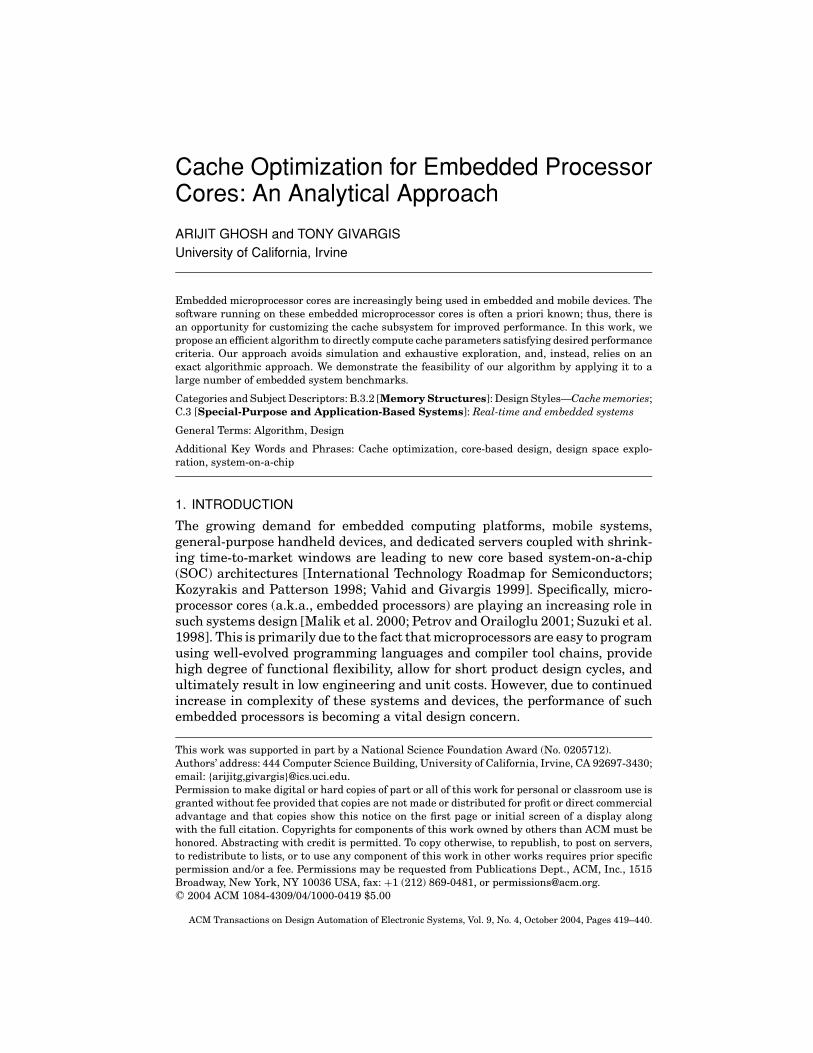
Finally, to build the RTS of the children, we follow the steps outlined inAlgorithm 7 (Figure 10).

3.4 Post-Processing Phase

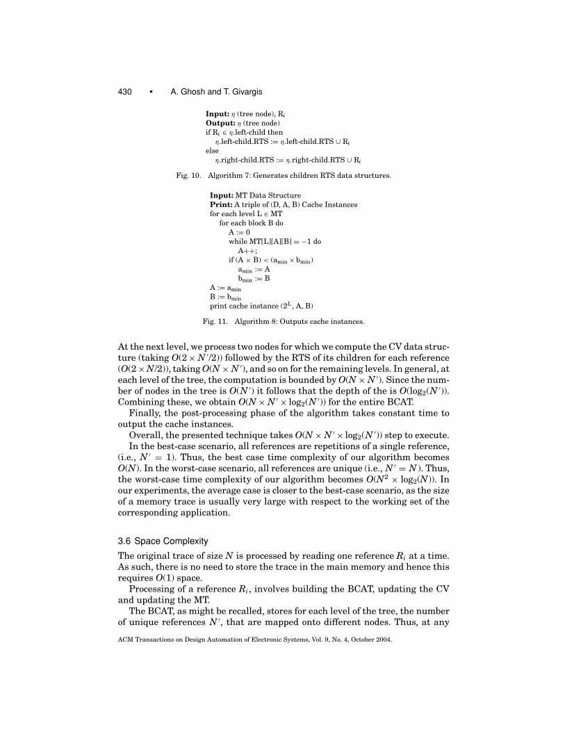
During the last phase of the algorithm, we read the MT data structure andoutput a set of triples consisting of cache depth, associativity and block sizethat satisfy the desired performance in terms of the number of cache misses,as shown in Algorithm 8.

In Algorithm 8 (Figure 11), for depths (number of rows) equal to 1, 2, 4, etc.,we print the optimal caches having the smallest degree of associativity andblock size to guarantee no more misses than the desired value K.



Input: CV, U j , RiOutput: CVfor Uk ∈ CV, k �= j do

if (CV[Uk] < CV[U j ])CV[Uk] = CV[Uk] + 1

CV[U j ] = i

Fig. 8. Algorithm 5: Updates the CV data structure.

Input: CV[U j ], K (desired misses), Ri , BInput: MT, L (tree level)Output: MTamax = i − CV[U j ] − 1;for A ∈ [1· · · amax] do

if (MT[L][A][B] ! = −1) && (MT[L][A][B] > K)MT[L][A][B] := −1 and break

MT[L][A][B] := MT[L][A][B] + 1

Fig. 9. Algorithm 6: Updates the MT data structure.

The number of optimal cache instances is no less than the minimum cachedepth for which associativity is equal to 1 and is no more than the width ofthe bus. This small set of cache instances can be further pruned by usingappropriate power, timing and/or area models to yield one final cache instancethat satisfies all design constraints.

3.5 Time Complexity

For time complexity analysis, we use the size of the trace N and the numberof unique references N ′ as the input parameters. We note that in most cases,N ′ is much smaller than N. Moreover, log2(N ′) is bounded by the width of thememory references (i.e., processor data-path), which is typically 32 or 64. Wehave shown the time complexity of each part of the algorithm in Figure 2, asexplained next.

The time taken to strip the trace amounts to sorting the references and thusis O(N × log2(N ′)).

The time taken to build the BCAT data structure is O(N ′ × log2(N ′)). Atthe root, we processes one node by looking at the N ′ unique references at acost of O(1 × N ′), at level one, we process two nodes by looking at N ′/2 uniquereferences at a cost of O(2 × N ′/2), at level two, we process four nodes by lookingat N ′/4 unique references at a cost of O(4 × N ′/4), etc. In general, at each levelof the tree, the computation is bounded by O(N ′). Since the number of nodesin the tree is O(N ′) it follows that the depth of the is O(log2(N ′)). Combiningthese, we obtain O(N ′log2(N ′)).

The time taken to build the MT data structure at each level of the BCAT isO(N × N ′) which is dominated by the computation involved in building the CVsof each node in BCAT. At the root, we process each reference (O(N)) by setting itsvalue in the CV and including it in the RTS of either the left or the right child.In addition, the entire length of CV needs to be traversed to account for repe-tition which takes O(N ′) time. The overall time at this level is thus O(N × N ′).



Input: η (tree node), RiOutput: η (tree node)if Ri ∈ η.left-child then

η.left-child.RTS := η.left-child.RTS ∪ Rielse

η.right-child.RTS := η.right-child.RTS ∪ Ri

Fig. 10. Algorithm 7: Generates children RTS data structures.

Input: MT Data StructurePrint: A triple of (D, A, B) Cache Instancesfor each level L ∈ MT

for each block B doA := 0while MT[L][A][B] = −1 do

A++;if (A × B) < (amin × bmin)

amin := Abmin := B

A := aminB := bminprint cache instance (2L, A, B)

Fig. 11. Algorithm 8: Outputs cache instances.

At the next level, we process two nodes for which we compute the CV data struc-ture (taking O(2 × N ′/2)) followed by the RTS of its children for each reference(O(2 × N/2)), taking O(N × N ′), and so on for the remaining levels. In general, ateach level of the tree, the computation is bounded by O(N × N ′). Since the num-ber of nodes in the tree is O(N ′) it follows that the depth of the is O(log2(N ′)).Combining these, we obtain O(N × N ′ × log2(N ′)) for the entire BCAT.

Finally, the post-processing phase of the algorithm takes constant time tooutput the cache instances.

Overall, the presented technique takes O(N × N ′ × log2(N ′)) step to execute.In the best-case scenario, all references are repetitions of a single reference,

(i.e., N ′ = 1). Thus, the best case time complexity of our algorithm becomesO(N). In the worst-case scenario, all references are unique (i.e., N ′ = N ). Thus,the worst-case time complexity of our algorithm becomes O(N2 × log2(N)). Inour experiments, the average case is closer to the best-case scenario, as the sizeof a memory trace is usually very large with respect to the working set of thecorresponding application.

3.6 Space Complexity

The original trace of size N is processed by reading one reference Ri at a time.As such, there is no need to store the trace in the main memory and hence thisrequires O(1) space.

Processing of a reference Ri, involves building the BCAT, updating the CVand updating the MT.

The BCAT, as might be recalled, stores for each level of the tree, the numberof unique references N ′, that are mapped onto different nodes. Thus, at any



given level, the worst-case memory requirement is O(N ′). If W is the bit-widthof the bus, then the number of levels in the tree is no more than W. As such,the worst-case memory requirement is O(W × N ′). However, as explained in thenext section, the BCAT is traversed in a depth-first fashion and no more thanone node per level is stored in the main memory at any given time. As such, theworst-case memory requirements is actually O(N ′).

The CV is an array of size N ′, and has thus a space complexity of O(N ′).Finally, the MT data structure has one entry for each possible cache depth. If

W is the bit-width of the bus, then this data structure requires a space of O(W).Since N ′ is considerably lesser than N and since W is typically equal to 32,

the space complexity of our algorithm is dominated by O(N ′).

3.7 Final Remarks

The data structure and algorithms described above are presented in a mannerto illustrate the logic and intuition behind our analytical cache optimizationtechnique. Here, we comment on issues to be considered in an actual imple-mentation (such as the one used to obtain the results in our experiments).

Stripping of a trace can be improved substantially by using a hash-tablestructure to keep track of unique reference. Moreover, the building of the MRCTdata structure can be performed during the stripping of the trace with no ad-ditional added time complexity if a hash-table is used.

The extensive use of sets in our technique is due to the fact that sets areefficient to represent, store, and manipulate on a computer system using bitvectors. In addition, the use of sets allows for execution of the algorithm on acluster of machines by utilizing a distributed set library, enabling the processingof very large trace files.

The implementation of Algorithm 1 and Algorithm 7 can be combined. Specif-ically, the BCAT does not need to be calculated in its entirety. Instead, a depthfirst traversal of the tree can be performed to reduce memory usage. Further,the data structures associated with each node can be deleted, after the nodehas been processed.

The advantage of our approach lies in the fact that the entire design space,obtained by varying the cache depth and associativity, can be exhaustivelyexplored in O(N × N ′ × log2(N ′)) time. Simulation of a single cache con-figuration requires O(N) time. As such, our approach is better suited foran exhaustive exploration of the complete design space. However, if the de-sign space is restricted by the limited values commonly used today for thecache parameters, then traditional simulation could be equally efficient forexploration.

4. EXPERIMENTS

For our experiments, we have used 16 typical embedded system applicationsthat are part of the PowerStone [Vahid and Givargis 1999] and the Media-Bench [Lee et al. 1997] benchmark applications. The applications include aJPEG decoder called jpeg, a modem decoder called v42, a Unix compression



Table VII. Data Trace Statistics

Total Unique TimeBenchmark Refs. N Refs. N′ (sec)adpcm 18431 381 2.7bcnt 456 162 0.11blit 4088 2027 6.879compress 58250 8906 466.87crc 2826 603 0.43des 20162 2241 19.268engine 211106 225 10.786fir 5608 146 0.39g3fax 229512 3781 221.098jpeg 1311693 39302 100576pocsag 13467 515 1.582qurt 503 84 0.07ucbqsort 61939 1144 17.516v42 649168 23942 15628toast 884700 1548 3942.92G723 1016262 173 281.77

utility called compress, a CRC checksum algorithm called crc, an encryptionalgorithm called des, an engine controller called engine, an FIR filter calledfir, a group three fax decoder called g3fax, a sorting algorithm called ucbqsort,an image rendering algorithm called blit, a POCSAG communication proto-col for paging applications called pocsag, an implementation of the EuropeanGSM 06.10 provisional standard for full-rate speech transcoding called toast, animplementation of the International Telegraph and Telephone ConsultativeCommittee (CCITT) G.723 voice compression called G723, and a few other em-bedded applications.

We first compiled and executed the benchmark applications on a MIPS R3000simulator. Our processor simulator is instrumented to output instruction/datamemory reference traces. The size of the traces N, the number of unique ref-erences N ′, and the execution time of our algorithm are reported for data andinstruction traces in Table VII and Table VIII, respectively.

We have ran these traces through our analytical algorithm for various valuesof desired number of cache misses K. Specifically, we have set K to one of 1%, 2%,3%, and 4% cache misses. For brevity, in Tables IX– XVIII, we have presentedthe optimal cache instances of the data and instruction traces for only five of thebenchmarks, namely des (Table IX, Table X), jpeg (Table XI, Table XII), g3fax(Table XIII, Table XIV), toast (Table XV, Table XVI), and g723 (Table XVII,Table XVIII). The correctness of the proposed approach has been verified bysubsequent cache simulation.

In these tables, the inner entries are the degree of associativity A and blocksize B necessary to ensure the desired number of cache misses. For example, if4% cache misses are allowed for the data trace of des, a eleven-way set associa-tive cache of block size 4 and depth 512 would suffice.

Our algorithm ran on a Pentium IV processor running at 2.8 GHz with 512MB of memory. The time taken to produce results for data/instruction traces isshown in the last columns of Table VII and Table VIII.



Table VIII. Instruction Trace Statistics

Total Unique TimeBenchmark Refs. N Refs. N′ (sec)adpcm 63255 611 12.689bcnt 1337 115 0.12blit 22244 149 0.781compress 137832 731 23.044crc 37084 176 1.653des 121648 570 22.954engine 409936 244 34.47fir 15645 327 1.60g3fax 1127387 220 67.73jpeg 4594120 623 693.876pocsag 47840 560 5.988qurt 1044 179 0.151ucbqsort 219710 321 17.165v42 2441985 656 389.856toast 3526594 7208 212501G723 4153844 71202 14575.8

Table IX. Optimal Instruction Cache Instances for des

Cache (Degree of Associativity)Depth (Desired Cache Misses K as a Percentage

D 1% 2% 3% 4%2 (541, 2) (541, 2) (541, 2) (541, 2)4 (271, 2) (271, 2) (271, 2) (271, 2)8 (136, 2) (136, 2) (136, 4) (136, 2)

16 (69, 2) (69, 2) (68, 2) (68, 2)32 (35, 2) (34, 2) (34, 2) (34, 2)64 (18, 2) (18, 2) (18, 2) (18, 2)

128 (10, 2) (10, 2) (10, 2) (9, 2)256 (5, 2) (5, 2) (5, 2) (5, 2)512 (3, 2) (3, 2) (3, 2) (3, 2)

1024 (2, 2) (2, 2) (2, 2) (2, 2)2048 (1, 2) (1, 2) (1, 2) (1, 2)

Table X. Optimal Data Cache Instances for des


D 1% 2% 3% 4%2 (1396, 2) (1300, 2) (1236, 2) (1179, 2)4 (1191, 2) (1124, 2) (1070, 2) (1035, 2)8 (1098, 2) (1043, 2) (1006, 2) (972, 2)

16 (352, 4) (326, 4) (309, 4) (296, 4)32 (176, 4) (163, 4) (155, 4) (148, 4)64 (88, 4) (82, 4) (78, 4) (75, 4)

128 (45, 4) (42, 4) (39, 4) (38, 4)256 (23, 4) (21, 4) (20, 4) (19, 4)512 (12, 4) (12, 4) (12, 4) (11, 4)

1024 (9, 4) (9, 4) (9, 2) (7, 2)2048 (5, 2) (5, 2) (5, 2) (4, 2)4096 (3, 2) (3, 2) (3, 2) (2, 2)8192 (2, 2) (2, 2) (2, 2) (1, 2)

16384 (1, 2) (1, 2) (1, 2) (1, 2)



Table XI. Optimal Instruction Cache Instances for jpeg


D 1% 2% 3% 4%2 (246, 2) (246, 2) (246, 2) (227, 2)4 (124, 2) (122, 2) (122, 2) (114, 2)8 (62, 2) (61, 2) (61, 2) (58, 2)

16 (31, 2) (31, 2) (30, 2) (30, 2)32 (17, 2) (15, 2) (15, 2) (15, 2)64 (8, 2) (8, 2) (8, 2) (8, 2)

128 (4, 2) (4, 2) (4, 2) (4, 2)256 (2, 2) (2, 2) (2, 2) (2, 2)512 (1, 2) (1, 2) (1, 2) (1, 2)

Table XII. Optimal Data Cache Instances for jpeg


D 1% 2% 3% 4%2 (38628, 2) (38615, 2) (38574, 2) (38493, 2)4 (38461, 2) (38461, 2) (38461, 2) (38430, 2)8 (19307, 2) (19245, 2) (19245, 2) (19216, 2)

16 (9654, 2) (9623, 2) (9622, 2) (9616, 2)32 (4828, 2) (4812, 2) (4811, 2) (4809, 16)64 (2414, 2) (2406, 2) (2405, 2) (2405, 2)

128 (1207, 2) (1203, 2) (1203, 2) (1202, 2)256 (603, 2) (602, 2) (601, 2) (601, 2)512 (302, 2) (301, 2) (301, 2) (301, 2)

1024 (151, 2) (151, 2) (150, 2) (150, 2)2048 (76, 2) (75, 2) (75, 2) (75, 2)4096 (38, 2) (38, 2) (38, 2) (38, 2)8192 (19, 2) (19, 2) (19, 2) (19, 2)

16384 (10, 2) (10, 2) (10, 2) (10, 2)32768 (5, 2) (5, 2) (5, 2) (5, 2)65536 (3, 2) (3, 2) (3, 2) (3, 2)

131072 (2, 2) (2, 2) (1, 2) (1, 2)262144 (1, 2) (1, 2) — —

Table XIII. Optimal Instruction Cache Instances for g3fax


D 1% 2% 3% 4%2 (87, 2) (87, 2) (87, 2) (83, 2)4 (44, 2) (43, 2) (43, 2) (41, 2)8 (24, 2) (22, 2) (21, 2) (21, 2)

16 (13, 2) (11, 2) (11, 2) (10, 2)32 (7, 2) (7, 2) (6, 2) (6, 2)64 (4, 2) (4, 2) (3, 2) (3, 2)

128 (3, 2) (2, 2) (2, 2) (2, 2)256 (2, 2) (2, 2) (2, 2) (2, 2)512 (1, 2) (1, 2) (1, 2) (1, 2)



Table XIV. Optimal Data Cache Instances for g3fax


D 1% 2% 3% 4%2 (1927, 2) (1920, 2) (1912, 2) (1902, 2)4 (965, 2) (961, 2) (955, 2) (950, 2)8 (485, 2) (481, 2) (478, 2) (476, 2)

16 (244, 2) (242, 2) (240, 2) (239, 2)32 (124, 2) (122, 2) (121, 2) (120, 2)64 (64, 2) (63, 2) (62, 2) (61, 2)

128 (35, 2) (33, 2) (32, 2) (31, 2)256 (19, 2) (17, 2) (17, 2) (16, 2)512 (10, 2) (9, 2) (8, 2) (8, 2)

1024 (5, 2) (5, 2) (5, 2) (4, 2)2048 (3, 2) (3, 2) (3, 2) (2, 2)4096 (2, 2) (2, 2) (2, 2) (1, 2)8192 (2, 2) (1, 2) (1, 2) —

16384 (1, 2) — — —

Table XV. Optimal Data Cache Instances for toast


D 1% 2% 3% 4%2 (5924, 2) (2283, 2) (2246, 2) (446, 2)4 (5924, 2) (2283, 2) (2246, 2) (446, 2)8 (5924, 2) (2283, 2) (2246, 2) (446, 2)

16 (5924, 2) (2283, 2) (2246, 2) (446, 2)32 (5924, 2) (2283, 2) (2246, 2) (446, 2)64 (5924, 2) (2283, 2) (2246, 2) (446, 2)

128 (5924, 2) (2283, 2) (2246, 2) (446, 2)256 (5924, 2) (2283, 2) (2246, 2) (446, 2)512 (5924, 2) (2283, 2) (2246, 2) (446, 2)

1024 (5924, 2) (2283, 2) (2246, 2) (446, 2)2048 (5924, 2) (2283, 2) (2246, 2) (446, 2)4096 (5924, 2) (2283, 2) (2246, 2) (446, 2)8192 (5924, 2) (2283, 2) (2246, 2) (446, 2)

16384 (5924, 2) (2283, 2) (2246, 2) (446, 2)32768 (5924, 2) (2283, 2) (2246, 2) (446, 2)65536 (2858, 2) (1203, 2) (1065, 2) (256, 2)

131072 (1447, 8) (615, 2) (514, 2) (256, 2)262144 (742, 8) (360, 8) (256, 16) (256, 2)524288 (379, 8) (313, 4) (256, 8) (256, 2)

1048576 (256, 8) (256, 4) (256, 8) (256, 2)2097152 (256, 4) (256, 2) (256, 4) (256, 2)4194304 (256, 4) (256, 2) (256, 4) (256, 2)8388608 (256, 2) (256, 2) (256, 2) (256, 2)

16777216 (128, 2) (128, 2) (128, 2) (128, 2)33554432 (64, 8) (64, 2) (64, 2) (64, 2)67108864 (32, 8) (32, 8) (32, 8) (32, 8)

134217728 (16, 8) (16, 8) (16, 8) (16, 8)268435456 (8, 8) (8, 8) (8, 8) (8, 8)536870912 (4, 8) (4, 8) (4, 8) (4, 8)

1073741824 (2, 8) (2, 8) (2, 8) (2, 8)2147483648 (1, 8) (1, 8) (1, 8) (1, 8)



Table XVI. Optimal Instruction Cache Instances for toast


D 1% 2% 3% 4%2 (1143, 2) (703, 2) (386, 2) (294, 2)4 (1143, 2) (703, 2) (386, 2) (294, 2)8 (1143, 2) (703, 2) (386, 2) (294, 2)

16 (1143, 2) (703, 2) (386, 2) (294, 2)32 (1143, 2) (703, 2) (386, 2) (294, 2)64 (1143, 2) (703, 2) (386, 2) (294, 2)

128 (1143, 2) (703, 2) (386, 2) (294, 2)256 (573, 2) (343, 4) (219, 2) (174, 2)512 (573, 2) (343, 4) (219, 2) (174, 2)

1024 (573, 2) (343, 2) (219, 2) (174, 2)2048 (573, 2) (343, 2) (219, 2) (174, 2)4096 (573, 2) (343, 2) (219, 2) (174, 2)8192 (573, 2) (343, 2) (219, 2) (174, 2)

16384 (573, 2) (343, 2) (219, 2) (174, 2)32768 (573, 2) (343, 2) (219, 2) (174, 2)65536 (278, 2) (170, 4) (128, 2) (104, 2)

131072 (162, 2) (112, 4) (98, 2) (75, 2)262144 (129, 8) (108, 2) (93, 2) (71, 2)524288 (128, 4) (108, 2) (89, 2) (61, 2)

1048576 (128, 4) (108, 2) (89, 2) (61, 2)2097152 (128, 2) (108, 2) (89, 2) (61, 2)4194304 (128, 2) (108, 2) (89, 2) (61, 2)8388608 (127, 2) (108, 2) (88, 2) (60, 2)

16777216 (108, 2) (94, 2) (77, 2) (59, 2)33554432 (54, 2) (51, 2) (41, 2) (33, 2)67108864 (27, 8) (26, 8) (21, 2) (16, 8)

134217728 (14, 8) (13, 8) (10, 16) (8, 8)268435456 (7, 8) (6, 8) (5, 8) (4, 8)536870912 (4, 8) (3, 8) (3, 8) (2, 8)

1073741824 (2, 8) (2, 8) (2, 8) (1, 8)2147483648 (1, 8) (1, 8) (1, 8) —

In Figure 12, we have plotted the average measured time taken to produceresults along with the analytical time complexity computed as N ×N ′×log2(N ′)on a logarithmic scale. As expected, the plots are consistent, with the actualtime taken asymptotically equal to the estimated time complexity.

As has been mentioned earlier, our approach is exact and in that respect, itis much faster compared to other exact methods like simulation. Our approachexplores a design space S that is exponential in size (where size is the size ofthe address space.) In other words, given a 32-bit address space, S containscache instances obtained by varying depth and associativity in every possibleway and block size from 2 to 32. Using existing cache simulation approachesin an exhaustive search algorithm will not terminate in reasonable amountof time. In order for us to provide comparison results, we limited the designspace (cache depth D from 64 to 1024, associativity A from 1 to 8 and block sizeB from 2 to 32 in powers of 2) and obtained the results for three benchmarkprograms(des, g3fax, blit), shown in Table XIX. Our approach still outperformedexisting approaches.



Table XVII. Optimal Data Cache Instances for G723


D 1% 2% 3% 4%2 (837, 2) (824, 2) (815, 2) (809, 2)4 (837, 2) (824, 2) (815, 2) (809, 2)8 (837, 2) (824, 2) (815, 2) (809, 2)

16 (837, 2) (824, 2) (815, 2) (809, 2)32 (837, 2) (824, 2) (815, 2) (809, 2)64 (837, 2) (824, 2) (815, 2) (809, 2)

128 (837, 2) (824, 2) (815, 2) (809, 2)256 (837, 2) (824, 2) (815, 2) (809, 2)512 (837, 2) (824, 2) (815, 2) (809, 2)

1024 (837, 2) (824, 2) (815, 2) (809, 2)2048 (837, 2) (824, 2) (815, 2) (809, 2)4096 (837, 2) (824, 2) (815, 2) (809, 2)8192 (837, 2) (824, 2) (815, 2) (809, 2)

16384 (837, 2) (824, 2) (815, 2) (809, 2)32768 (837, 2) (824, 2) (815, 2) (809, 2)65536 (429, 2) (415, 2) (409, 2) (409, 2)

131072 (272, 4) (262, 2) (258, 4) (259, 2)262144 (210, 4) (196, 4) (193, 4) (191, 4)524288 (210, 2) (196, 2) (193, 2) (191, 2)

1048576 (210, 2) (196, 2) (193, 2) (191, 2)2097152 (210, 2) (196, 2) (193, 2) (191, 2)4194304 (210, 2) (196, 2) (193, 2) (191, 2)8388608 (210, 2) (196, 2) (193, 2) (191, 2)

16777216 (105, 2) (98, 2) (96, 2) (95, 2)33554432 (53, 2) (50, 2) (48, 2) (48, 2)67108864 (26, 8) (25, 8) (25, 2) (24, 8)

134217728 (14, 8) (13, 8) (12, 8) (12, 8)268435456 (7, 8) (7, 8) (7, 8) (6, 8)536870912 (4, 8) (4, 8) (4, 8) (3, 8)

1073741824 (2, 8) (2, 8) (2, 8) (2, 8)2147483648 (1, 8) (1, 8) (1, 8) (1, 8)

5. FUTURE WORK

The focus of our current work is on core-based system-on-chip design, wherethe processor core, main memory controller core etc are assumed to be fixed. Assuch, we explore the design space parameterized by associativity, block size andcache size. In order to provide an analytical framework that encompasses moredesign parameters, in the future we intend to incorporate such design param-eters as different replacement policies, multilevel caches, and bus architectureeffects.

6. CONCLUSION

We have proposed an efficient algorithm to directly compute cache parameterssatisfying desired performance criteria. The proposed approach avoids simu-lation and exhaustive exploration. Here, we consider a design space that isformed by varying cache size, degree of associativity and block size. For a given



Table XVIII. Optimal Instruction Cache Instances for G723


D 1% 2% 3% 4%2 (103, 2) (100, 2) (99, 2) (98, 2)4 (103, 2) (100, 2) (99, 2) (98, 2)8 (103, 2) (100, 2) (99, 2) (98, 2)

16 (103, 2) (100, 2) (99, 2) (98, 2)32 (103, 2) (100, 2) (99, 2) (98, 2)64 (103, 2) (100, 2) (99, 2) (98, 2)

128 (103, 2) (100, 2) (99, 2) (98, 2)256 (77, 2) (76, 2) (75, 2) (75, 2)512 (77, 2) (76, 2) (75, 2) (75, 2)

1024 (77, 2) (76, 2) (75, 2) (75, 2)2048 (77, 2) (76, 2) (75, 2) (75, 2)4096 (77, 2) (76, 2) (75, 2) (75, 2)8192 (77, 2) (76, 2) (75, 2) (75, 2)

16384 (77, 2) (76, 2) (75, 2) (75, 2)32768 (77, 2) (76, 2) (75, 2) (75, 2)65536 (65, 2) (64, 2) (63, 2) (63, 2)

131072 (65, 2) (64, 2) (63, 2) (63, 2)262144 (65, 4) (64, 2) (63, 2) (63, 4)524288 (65, 4) (64, 4) (63, 2) (63, 4)

1048576 (65, 4) (64, 4) (63, 4) (63, 4)2097152 (65, 4) (64, 2) (63, 4) (63, 2)4194304 (65, 2) (64, 2) (63, 2) (63, 2)8388608 (65, 2) (64, 2) (63, 2) (63, 2)

16777216 (64, 2) (64, 2) (63, 2) (63, 2)33554432 (45, 2) (45, 2) (45, 2) (43, 2)67108864 (24, 8) (23, 8) (21, 8) (21, 2)

134217728 (12, 8) (12, 8) (11, 8) (11, 8)268435456 (7, 8) (6, 8) (6, 8) (5, 8)536870912 (3, 8) (3, 8) (3, 8) (3, 8)

1073741824 (2, 8) (2, 8) (2, 8) (2, 8)2147483648 (1, 8) (18, 8) (1, 8) (1, 8)

Fig. 12. Analytical time complexity vs. actual run times.



Table XIX. Comparison with Simulation

AnalyticalApproach Simulation

(sec) (sec)des 0.02 100g3fax 2 900blit 0.004 20

memory reference trace, our algorithm takes as input the design constraintin the form of the number of desired cache misses and outputs a set of opti-mal cache instances that meet the constraint. The feasibility of the proposedapproach has been verified experimentally using the PowerStone and Media-bench benchmarks.

REFERENCES

BAER, J. AND WANG, W. 1998. On the inclusion properties for multi-level cache hierarchies. InProceedings of the International Conference on Computer Architecture.

BALASUBRAMONIAN, R., ALBONESI, D., BUYUKTOSUNOGLU, A., AND DWARKADAS, S. 2000. Memory hier-archy reconfiguration for energy and performance in general-purpose processor architectures. InProceedings of the International Symposium on Microarchitecture.

HARPER, J., KERBYSON, D., AND NUDD, G. 1999. Analytical modeling of set-associative cache behav-ior. IEEE Trans. Comput. 48, 10 (Oct.), 1009–1024.

HILL, M. 1987. Aspects of cache memory and instruction buffer performance. Ph.D. dissertation.University of California, Berkeley, Berkeley, Calif.

INTEL PENTIUM IV. ftp://download.intel.com/design/Pentium4/manuals/24896609.pdf.INTERNATIONAL TECHNOLOGY ROADMAP FOR SEMICONDUCTORS. public.itrs.net.KIROVSKI, D., LEE, C., POTKONJAK, M., AND MANGIONE-SMITH, W. 1998. Synthesis of power efficient

systems-on-silicon. In Proceedings of Asian South Pacific Design Automation Conference.KOZYRAKIS, C. AND PATTERSON, D. 1998. A new direction for computer architecture research. IEEE

Comput. 31, 11 (Nov.), 24–32.LAJOLO, M., RAGHUNATHAN, A., DEY, S., LAVAGNO, L., AND SANGIOVANNI-VINCENTELLI, A. 1999. Effi-

cient power estimation techniques for HW/SW systems. In Proceedings of IEEE Alessandro VoltaMemorial Workshop on Low-Power Design. IEEE Computer Society Press, Los Alamitos, Calif.

LEE, C., POTKONJAK, M., AND MANGIONE-SMITH, W. 1997. MediaBench: A tool for evaluating andsynthesizing multimedia and communications systems. In Proceedings of the International Sym-posium on Microarchitecture.

LI, Y. AND HENKEL, J. 1998. A framework for estimating and minimizing energy dissipation ofembedded HW/SW systems. In Proceedings of the Design Automation Conference.

BREHOB, M. AND ENBODY, R. J. 1996. An analytical model of locality and caching. Tech. rep.,Michigan State University.

MALIK, A., MOYER, B., AND CERMAK, D. 2000. A lower power unified cache architecture providingpower and performance flexibility. In Proceedings of the International Symposium on Low PowerElectronics and Design.

MATTSON, R., GECSEI, J., SLUTZ, D., AND TRAIGER, I. 1970. Evaluation techniques for storage hier-archies. IBM Syst. J. 9, 2.

MOTOROLA MPC500. http://e www.motorola.com/files/platforms/doc/ref manual/MGT560RM.pdf.MOTOROLA MPC5200. http://e www.motorola.com/files/32bit/doc/ref manual/G2CORERM.pdf.MOTOROLA MPC823. http://e-www.motorola.com/files/if/cnb/MPC823UM.pdf.PETROV, P. AND ORAILOGLU, A. 2001. Towards effective embedded processors in codesigns: Cus-

tomizable partitioned caches. In Proceedings of the International Workshop on HW/SW Codesign.SATO, T. 2000. Evaluating trace cache on moderate-scale processors. IEEE Comput. 147, 6 (Nov),

369–374.



SHIUE, W. AND CHAKRABARTI, C. 1999. Memory exploration for low power embedded systems. InProceedings of the Design Automation Conference.

SU, C. AND DESPAIN, A. 1995. Cache design trade-offs for power and performance optimization: Acase study. In Proceedings of the International Symposium on Low Power Electronics and Design.

SUZUKI, K., ARAI, T., AND KOUHEI, N. 1998. V830R/AV: Embedded multimedia superscalar RISCprocessor. IEEE Micro 18, 2 (Mar.), 36–47.

VAHID, F., AND GIVARGIS, T. 1999. The case for a configure-and-execute paradigm. In Proceedingsof the International Symposium on Low Power Electronics and Design.

WILTON, S. AND JOUPPI, N. 1996. CACTI: An enhanced cache access and cycle time model. IEEEJ. Solid State Circ. 31, 5 (May), 677–688.

WU, Z. AND WOLF, W. 1999. Iterative cache simulation of embedded CPUs with trace stripping.In Proceedings of International Workshop on HW/SW Codesign.

Received April 2003; revised January 2004 and May 2004; accepted June 2004


Cache Optimization for Embedded Processor Cores: An...

Documents

Transcript of Cache Optimization for Embedded Processor Cores: An...