Cabauw Experimental Results from the Project for ...

1194 VOLUME 10J O U R N A L O F C L I M A T E

q 1997 American Meteorological Society

Cabauw Experimental Results from the Project for Intercomparison of Land-SurfaceParameterization Schemes

T. H. CHEN,a A. HENDERSON-SELLERS,a P. C. D. MILLY,b A. J. PITMAN,a A. C. M. BELJAARS,c J. POLCHER,d

F. ABRAMOPOULOS,e A. BOONE,f S. CHANG,g F. CHEN,h Y. DAI,i C. E. DESBOROUGH,a R. E. DICKINSON,j

L. DUMENIL,k M. EK,c J. R. GARRATT,l N. GEDNEY,m Y. M. GUSEV,n J. KIM,o R. KOSTER,p E. A. KOWALCZYK,l

K. LAVAL,d J. LEAN,q D. LETTENMAIER,r X. LIANG,s J.-F. MAHFOUF,t H.-T. MENGELKAMP,u K. MITCHELL,h

O. N. NASONOVA,n J. NOILHAN,v A. ROBOCK,w C. ROSENZWEIG,e J. SCHAAKE,x C. A. SCHLOSSER,w

J.-P. SCHULZ,k Y. SHAO,y A. B. SHMAKIN,z D. L. VERSEGHY,aa P. WETZEL,f E. F. WOOD,s Y. XUE,bb

Z.-L. YANG,j AND Q. ZENGi

aClimatic Impacts Centre, Macquarie University, Sydney, AustraliabU.S. Geological Survey and Geophysical Fluid Dynamics Laboratory/NOAA, Princeton, New Jersey

cRoyal Netherlands Meteorological Institute, De Bilt, the NetherlandsdLaboratoire de Meteorologie Dynamique du CNRS, Paris, France

eScience Systems and Applications Incorporated, New York City, New YorkfMesoscale Dynamics and Precipitation Branch, NASA/Goddard Space Flight Center, Greenbelt, Maryland

gPhillips Laboratory (PL/GPAB), Hanscom AFB, MassachusettshDevelopment Division, National Centers for Environmental Prediction, NOAA, Camp Springs, Maryland

iInstitute of Atmospheric Physics, Academy of Science, Beijing, People’s Republic of ChinajInstitute of Atmospheric Physics, The University of Arizona, Tucson, Arizona

kMax-Planck-Institut fur Meteorologie, Hamburg, GermanylDivision of Atmospheric Research, CSIRO, Aspendale, Victoria, AustraliamMeteorology Department, Reading University, Reading, United Kingdom

nInstitute of Water Problems, Moscow, RussiaoLawrence Livermore National Laboratory, Livermore, California

pHydrological Sciences Branch, NASA/GSFC, Greenbelt, MarylandqHadley Centre for Climate Prediction and Research, Meteorological Office, Berkshire, United Kingdom

rDepartment of Civil Engineering, University of Washington, Seattle, WashingtonsDepartment of Civil Engineering and Operations Research, Princeton University, Princeton, New Jersey

tECMWF, Reading, United KingdomuInstitute for Atmospheric Physics, GKSS–Research Center, Max-Planck-Strasse, Geesthacht, Germany

vMeteo-France/CNRM, Toulouse, FrancewDepartment of Meteorology, University of Maryland at College Park, College Park, Maryland

xOffice of Hydrology, NWS/NOAA, Silver Spring, MarylandyCentre for Advanced Numerical Computation in Engineering and Science, University of New South Wales, Sydney, Australia

zInstitute of Geography, Moscow, RussiaaaClimate Research Branch, Atmospheric Environment Service, Downsview, Ontario, Canada

bbCentre for Ocean–Land–Atmosphere Studies, Calverton, Maryland

(Manuscript received 18 December 1995, in final form 2 May 1996)

ABSTRACT

In the Project for Intercomparison of Land-Surface Parameterization Schemes phase 2a experiment, meteo-rological data for the year 1987 from Cabauw, the Netherlands, were used as inputs to 23 land-surface fluxschemes designed for use in climate and weather models. Schemes were evaluated by comparing their outputswith long-term measurements of surface sensible heat fluxes into the atmosphere and the ground, and of upwardlongwave radiation and total net radiative fluxes, and also comparing them with latent heat fluxes derived froma surface energy balance. Tuning of schemes by use of the observed flux data was not permitted. On an annualbasis, the predicted surface radiative temperature exhibits a range of 2 K across schemes, consistent with therange of about 10 W m22 in predicted surface net radiation. Most modeled values of monthly net radiation differfrom the observations by less than the estimated maximum monthly observational error (610 W m22). However,modeled radiative surface temperature appears to have a systematic positive bias in most schemes; this mightbe explained by an error in assumed emissivity and by models’ neglect of canopy thermal heterogeneity. Annualmeans of sensible and latent heat fluxes, into which net radiation is partitioned, have ranges across schemes of

Corresponding author address: Dr. Tian Hong Chen, Australian Oceanographic Data Centre, Maritime Headquarters, Potts Point, NSW2001, Australia.E-mail: [email protected]

JUNE 1997 1195C H E N E T A L .

30 W m22 and 25 W m22, respectively. Annual totals of evapotranspiration and runoff, into which the precipitationis partitioned, both have ranges of 315 mm. These ranges in annual heat and water fluxes were approximatelyhalved upon exclusion of the three schemes that have no stomatal resistance under non-water-stressed conditions.Many schemes tend to underestimate latent heat flux and overestimate sensible heat flux in summer, with areverse tendency in winter. For six schemes, root-mean-square deviations of predictions from monthly obser-vations are less than the estimated upper bounds on observation errors (5 W m22 for sensible heat flux and 10W m22 for latent heat flux). Actual runoff at the site is believed to be dominated by vertical drainage togroundwater, but several schemes produced significant amounts of runoff as overland flow or interflow. Thereis a range across schemes of 184 mm (40% of total pore volume) in the simulated annual mean root-zone soilmoisture. Unfortunately, no measurements of soil moisture were available for model evaluation. A theoreticalanalysis suggested that differences in boundary conditions used in various schemes are not sufficient to explainthe large variance in soil moisture. However, many of the extreme values of soil moisture could be explainedin terms of the particulars of experimental setup or excessive evapotranspiration.

1. Introduction

Project for Intercomparison of Land-Surface Param-eterization Schemes (PILPS) is a World Climate Re-search Programme project operating under the auspicesof the Global Energy and Water Cycle Experiment andthe Working Group on Numerical Experimentation. Itsgoal is to improve understanding of the parameterizationof interactions between the atmosphere and the conti-nental surface in climate and weather forecast models.Since its establishment in 1992, PILPS has been re-sponsible for a number of complementary sensitivitystudies. In phase 1 of the project (Pitman et al. 1993),land-surface schemes were compared off-line using at-mospheric forcing generated from a general circulationmodel, thereby preventing feedbacks between the at-mosphere and the surface. Phase 2a, described in thispaper, was again off-line, but observed point data fromCabauw, the Netherlands (518589N, 48569E), were usedas the atmospheric forcing. Furthermore, observed fluxdata were available for evaluation of the performanceof the schemes. The phase 2a experiment was the firstone in which observational data were used in PILPS(Henderson-Sellers et al. 1995), and the aim was todetermine how well individual land-surface schemescould reproduce a set of flux measurements at the Ca-bauw site taken coincidentally with the measurementsof the atmospheric forcing.

Twenty-three land-surface schemes (Tables 1 and 2)participated in the PILPS phase 2a experiment. The fo-cus of this study will be on a community-wide inter-comparison among schemes, rather than on detailedanalysis of individuals. The presentation of the exper-imental results is organized as follows. The observa-tional data will be described in section 2. The experi-mental design and the underlying philosophy will bediscussed in section 3, and the experimental results willbe investigated in section 4. Finally, concluding remarkswill be given in section 5. An appendix contains detailsof the Cabauw site characteristics and parameter setup.

2. Cabauw observational data

Rigorous testing of land-surface schemes requires ac-curate and contemporaneous observations of the input

variables (henceforth ‘‘atmospheric forcing,’’ which in-cludes downward shortwave and longwave radiation,precipitation, surface atmospheric pressure, and near-surface air humidity, temperature, and wind speed),prognostic variables (surface temperatures and waterstores), and output variables (net shortwave and long-wave radiation, latent heat flux, sensible heat flux,ground heat flux, evapotranspiration, and runoff) of theschemes. Due to the importance of seasonal storage inthe soil for water balance, and because of the largesystematic changes in water and energy balancesthrough the year, it is preferred to have at least 1 yearof data. Although no available dataset was ideal forPILPS, several sets were sufficiently comprehensive towarrant consideration.

The Cabauw dataset was chosen for the PILPS phase2a experiment for three reasons. First, it was plannedwithin the PILPS framework to test land-surfaceschemes with different datasets representative of dif-ferent land-surface conditions—Cabauw was a usefulcase study for midlatitude homogeneous grassland. Sec-ond, at Cabauw, deep soil is saturated throughout theyear and evapotranspiration is seldom limited by watersupply; this facilitates analysis of model outputs underthe non-water-stressed condition, which is an importantlimiting case. It was anticipated that these two featuresof the Cabauw site might obviate some causes of thedivergence among numerical simulations: the variabilityin water-storage time constants across schemes (Yanget al. 1995) and the variability in root-zone soil moistureacross schemes (Shao et al. 1994). At the same time,of course, the rarity of water stress implies that theCabauw data do not provide a good test of the models’ability to function when the water supply is limited.Finally, the Cabauw data include 1 full year of surfacelatent heat and sensible heat fluxes, providing a basisfor testing model performance in terms of seasonal vari-ation; many of the other available datasets, such as theHydrological Atmospheric Pilot Experiment–Modelis-ation du Bilan Hydrique (Goutorbe and Tarrieu 1991),have these fluxes only for limited periods of time.

The Cabauw site consists mainly of short grass di-vided by narrow ditches. The climate in the area is char-acterized as ‘‘moderate maritime,’’ with a prevailing


TA

BL

E1.

Lis

tof

land

-sur

face

sche

mes

part

icip

atin

gin

PIL

PS

phas

e2a

and

som

eba

sic

info

rmat

ion

abou

tth

em.

Mod

elC

onta

ct

Num

ber

ofla

yers

for

Ca

Tb

Sc

Rd

Tim

est

epS

pinu

pti

me

Maj

orpu

rpos

e

Phi

loso

phy

for

Ca

Tb

Sc

Ref

eren

ce

BA

SE

C.E

.D

esbo

roug

hA

.J.

Pit

man

13

33

20m

in5

yrG

CM

Aer

odyn

amic

Hea

tdi

ffus

ion

Phi

lip–

deV

ries

—

BA

TS

R.E

.D

icki

nson

Z.-

L.

Yan

g1

23

230

min

3yr

GC

MP

enm

an–

Mon

teit

hF

orce

-re

stor

eD

arcy

’sla

wD

icki

nson

etal

.(1

986,

1993

)

BU

CK

C.A

.S

chlo

sser

A.

Rob

ock

01

11

30m

in1

yrG

CM

Impl

icit

Hea

tba

lanc

eB

ucke

teM

anab

e(1

969)

Rob

ock

etal

.(1

995)

CA

PS

S.

Cha

nge

M.

Ek

13

32

30m

in1

yrG

CM

Pen

man

–M

onte

ith

Hea

tdi

ffus

ion

Dar

cy’s

law

Mah

rtan

dP

an(1

984)

Pan

and

Mah

rt(1

987)

CA

PS

LL

NL

J.K

im1

23

15

min

10yr

GC

Mm

esos

cale

Pen

man

–M

onte

ith

Hea

tdi

ffus

ion

Dif

fusi

onM

ahrt

and

Pan

(198

4)K

iman

dE

k(1

995)

CA

PS

NM

CK

.M

itch

ell

F.C

hen

13

32

30m

in3

yrG

CM

mes

osca

leP

enm

an–

Mon

teit

hH

eat

diff

usio

nD

arcy

’sla

wM

ahrt

and

Pan

(198

4)P

anan

dM

ahrt

(198

7)C

hen

etal

.(1

996)

CL

AS

SD

.V

erse

ghy

13

33

30m

in3

yrG

CM

Pen

man

–M

onte

ith

Hea

tdi

ffus

ion

Dar

cy’s

law

Ver

segh

y(1

991)

Ver

segh

yet

al.

(199

3)C

SIR

O9

E.A

.K

owal

czyk

J.R

.G

arra

tt1

32

130

min

2yr

GC

MA

erod

ynam

icH

eat

diff

usio

nF

orce

–res

tore

Kow

alcz

yket

al.

(199

1)

EC

HA

ML

.D

umen

ilJ.

-P.

Sch

ulz

15

11

30m

in5

yrG

CM

Aer

odyn

amic

Hea

tdi

ffus

ion

Buc

kete

Dum

enil

and

Todi

ni(1

992)

GIS

SF.

Abr

amop

oulo

sC

.R

osen

zwei

g1

66

630

min

13yr

GC

MA

erod

ynam

icH

eat

diff

usio

nD

arcy

’sla

wA

bram

opou

los

etal

.(1

988)

Ros

enzw

eig

and

Abr

amop

oulo

s(1

991)

IAP

94Q

.Z

eng

Y.

Dai

13

32

60m

in60

yrG

CM

Pen

man

–M

onte

ith

Hea

tdi

ffus

ion

Dar

cy’s

law

—

ISB

AJ.

Noi

lhan

J.-F

.M

ahfo

uf1

22

15

min

1yr

GC

Mm

esos

cale

Aer

odyn

amic

For

ce–

rest

ore

For

ce–r

esto

reN

oilh

anan

dP

lant

on(1

989)

MO

SA

ICR

.K

oste

r1

23

25

min

6yr

GC

MP

enm

an–

Mon

teit

hF

orce

–re

stor

eD

arcy

’sla

wK

oste

ran

dS

uare

z(1

992)

PL

AC

EP.

Wet

zel

A.

Boo

ne1

750

230

min

3yr

Fle

xibl

eA

erod

ynam

icH

eat

diff

usio

nD

arcy

’sla

wW

etze

lan

dB

oone

(199

5)

SE

CH

IBA

2J.

Pol

cher

K.

Lav

al1

72

130

min

2yr

GC

MA

erod

ynam

icH

eat

diff

usio

nC

hois

nel

Duc

oudr

eet

al.

(199

3)

SE

WA

BH

.-T.

Men

gelk

amp

16

61

10–3

0se

c3

yrM

esos

cale

Aer

odyn

amic

Hea

tdi

ffus

ion

Dif

fusi

on—

SP

ON

SO

RA

.B.

Shm

akin

11

22

24hr

3yr

GC

MA

erod

ynam

icE

nerg

yba

lanc

eB

ucke

teS

hmak

inet

al.

(199

3)S

SiB

Y.

Xue

C.A

.S

chlo

sser

12

31

30m

in2

yrG

CM

mes

osca

leP

enm

an–

Mon

teit

hF

orce

–re

stor

eD

iffu

sion

Xue

etal

.(1

991)

SW

AP

Y.M

.G

usev

O.

N.

Nas

onov

a1

21

124

hr2

yrM

esos

cale

Aer

odyn

amic

Hea

tdi

ffus

ion

Buc

kete

—

SW

BJ.

Sch

aake

V.

Kor

en0

32

230

min

3yr

Mes

osca

le—

Hea

tdi

ffus

ion

Buc

kete

Sch

aake

etal

.(1

995)

UG

AM

PN

.G

edne

y1

33

230

min

14yr

GC

MP

enm

an–

Mon

teit

hH

eat

diff

usio

nD

arcy

’sla

w—

UK

MO

J.L

ean

14

44

30m

in1

yrG

CM

Pen

man

-M

onte

ith

Hea

tdi

ffus

ion

Dar

cy’s

law

War

rilo

wet

al.

(198

6)G

rego

ryan

dS

mit

h(1

994)

VIC

-3L

X.

Lia

ngE

.W

ood

D.

Let

tenm

aier

12

32

60m

in2

yrG

CM

mes

osca

leP

enm

an–

Mon

teit

hH

eat

diff

usio

nca

paci

tyan

dm

ore

Var

iabl

ein

filt

rati

onL

iang

eet

al.

(199

4)L

iang

etal

.(1

996)

aC

anop

y.b

Soi

lte

mpe

ratu

re.

cS

oil

moi

stur

e.d

Roo

ts.

eB

ucke

tpl

usva

riat

ion.

JUNE 1997 1197C H E N E T A L .

TABLE 2. Explanations of scheme acronyms.

Acronym Explanation

BASE Best Approximation of Surface ExchangesBATS Biosphere Atmosphere Transfer SchemeBUCK BucketCAPS Coupled Atmosphere–Plant Soil modelCAPSLLNL Coupled Atmosphere–Plant Soil model, Lawrence

Livermore National Laboratory versionCAPSNMC Coupled Atmosphere–Plant Soil model, National

Meteorological Center (currently known as theNational Centers for Environmental Prediction)version

CLASS Canadian Land Surface SchemeCSIRO9 CSIRO Soil-Canopy Scheme, nine-level GCM

versionECHAM Land Surface Scheme of the ECHAM General

Circulation ModelGISS GISS Ground Hydrology ModelIAP94 Institute of Atmospheric Physics Land Surface

Physical Processes Model for AtmosphericGeneral Circulation Model, version 1994

ISBA Interaction Soil Biosphere AtmosphereMOSAIC MosaicPLACE Parameterization for Land–Atmosphere–Cloud

ExchangeSECHIBA2 Schematisation des Echanges Hydriques Interface

Biosphere–Atmosphere, version 2SEWAB Surface Energy and Water Balance schemeSPONSOR Semi-distributed Parameterization Scheme of the

Orography-Induced MacrohydrologySSiB Simplified Simple Biosphere ModelSWAP Soil Water–Atmosphere–PlantSWB Simple Water Balance ModelUGAMP University Global Atmospheric Modelling Pro-

gramUKMO The U.K. Meteorological Office Land Surface

SchemeVIC-3L Three-Layer Variable Infiltration Capacity Scheme

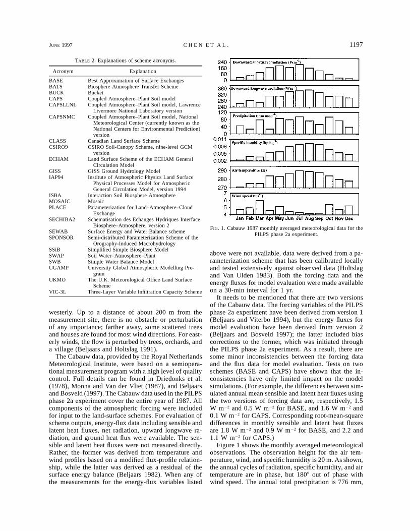
FIG. 1. Cabauw 1987 monthly averaged meteorological data for thePILPS phase 2a experiment.

westerly. Up to a distance of about 200 m from themeasurement site, there is no obstacle or perturbationof any importance; farther away, some scattered treesand houses are found for most wind directions. For east-erly winds, the flow is perturbed by trees, orchards, anda village (Beljaars and Holtslag 1991).

The Cabauw data, provided by the Royal NetherlandsMeteorological Institute, were based on a semiopera-tional measurement program with a high level of qualitycontrol. Full details can be found in Driedonks et al.(1978), Monna and Van der Vliet (1987), and Beljaarsand Bosveld (1997). The Cabauw data used in the PILPSphase 2a experiment cover the entire year of 1987. Allcomponents of the atmospheric forcing were includedfor input to the land-surface schemes. For evaluation ofscheme outputs, energy-flux data including sensible andlatent heat fluxes, net radiation, upward longwave ra-diation, and ground heat flux were available. The sen-sible and latent heat fluxes were not measured directly.Rather, the former was derived from temperature andwind profiles based on a modified flux-profile relation-ship, while the latter was derived as a residual of thesurface energy balance (Beljaars 1982). When any ofthe measurements for the energy-flux variables listed

above were not available, data were derived from a pa-rameterization scheme that has been calibrated locallyand tested extensively against observed data (Holtslagand Van Ulden 1983). Both the forcing data and theenergy fluxes for model evaluation were made availableon a 30-min interval for 1 yr.

It needs to be mentioned that there are two versionsof the Cabauw data. The forcing variables of the PILPSphase 2a experiment have been derived from version 1(Beljaars and Viterbo 1994), but the energy fluxes formodel evaluation have been derived from version 2(Beljaars and Bosveld 1997); the latter included biascorrections to the former, which was initiated throughthe PILPS phase 2a experiment. As a result, there aresome minor inconsistencies between the forcing dataand the flux data for model evaluation. Tests on twoschemes (BASE and CAPS) have shown that the in-consistencies have only limited impact on the modelsimulations. (For example, the differences between sim-ulated annual mean sensible and latent heat fluxes usingthe two versions of forcing data are, respectively, 1.5W m22 and 0.5 W m22 for BASE, and 1.6 W m22 and0.1 W m22 for CAPS. Corresponding root-mean-squaredifferences in monthly sensible and latent heat fluxesare 1.8 W m22 and 0.9 W m22 for BASE, and 2.2 and1.1 W m22 for CAPS.)

Figure 1 shows the monthly averaged meteorologicalobservations. The observation height for the air tem-perature, wind, and specific humidity is 20 m. As shown,the annual cycles of radiation, specific humidity, and airtemperature are in phase, but 1808 out of phase withwind speed. The annual total precipitation is 776 mm,


10% above the climatological mean, and the annualmean air temperature is 282 K, 0.5 K below the cli-matological mean, indicating that 1987 was slightly wet-ter and cooler than average at Cabauw.

Estimation of the accuracy of the observed data is animportant issue. There are a number of sources of errorin the Cabauw data: the measurements themselves, thealgorithm used to derive the sensible heat flux frommeasured variables, the substitution of data from a near-by synoptic station (De Bilt, 30 km away) for mea-surement gaps (due to instrument failure or data trans-mission problems), and errors in the parameterizationscheme used to synthesize the missing energy fluxes formodel evaluation. Beljaars and Bosveld (1997) haveassessed the quality of the Cabauw dataset. They sug-gested that precipitation (the most difficult observationamong the meteorological forcing variables) is possiblyunderestimated by 2%–11%, depending on wind. Byexploiting the redundancy in observations and by com-paring simulated data and observations when both areavailable, they subjectively estimated the range of erroron monthly averages to be 65 W m22 for sensible heatflux, 610 W m22 for both latent heat flux and net ra-diation, and 61 W m22 for ground heat flux at thesurface. The ranges of observation error quoted herepertain to the maximum monthly mean differences be-tween methods. In the evaluation of models, departuresof model outputs from observations were consideredsignificant if they fell outside these ranges.

Another discrepancy between simulations and obser-vations is one of scale. This problem has not been tack-led here—the assumption is made that PILPS’s simu-lations are comparable with point observations. Thisassumption is justified, in part, by a survey distributedin 1992, in reply to which many modelers asserted thattheir land-surface schemes were independent of scale(Henderson-Sellers and Brown 1992). However, it isrecognized that the scale issue could be the cause ofsome (perhaps many) of the discrepancies reported inthis paper. Additionally, the approximation was madethat 1987 was an equilibrium year (with identical initialand final states). The error induced by this approxi-mation is expected to be limited in a very wet (and,presumably, short memory) system, such as the Cabauwsite.

3. Design of numerical experiment

In accordance with the assumption that 1987 was anequilibrium year, each scheme was run using the ob-served 1987 forcing and repeated a sufficient numberof times for the scheme to reach a dynamic equilibrium(defined below). For a lower boundary condition onwater transfer, it was specified that a water table waspresent at 1-m depth. (This information was not usedby all schemes, as discussed in a later section.) Deepvertical heat flux was taken to be negligible in all

schemes. All schemes were initialized by saturating allliquid water stores and setting all temperatures to 279 K.

Equilibrium was defined as being the first occasionon which the January mean values of surface radiativetemperature, latent and sensible heat fluxes, and root-zone soil moisture did not change by more than 0.01K, 0.1 W m22, and 0.1 mm, respectively, from year Nto year N 1 1; the equilibration time was then N years.Actual spinup time n ($ N) allowed by individualschemes is given in Table 1.

All land-surface schemes in the phase 2a experimentrequire virtually identical forcing variables, but theirrequirements for input parameters characterizing theland-surface differ in several respects (Polcher et al.1996). For example, soil-water storage and release maybe treated in one scheme using concepts of water po-tential and hydraulic conductivity, but in another schemeusing the simpler concept of a lumped storage reservoir.The need to ensure consistency in the assignment ofparameters (e.g., leaf area index, soil depth, albedo, andsurface roughness) across schemes is a fundamental andcontinuing challenge in PILPS. The general approachtaken was to describe the site physically in as muchdetail as possible and to assign parameters based on thatphysical description. In many cases, the detailed de-scription was derived not from site-specific estimates,but from preexisting vegetation- and soil-dependent pa-rameter tables in the more detailed land-surfaceschemes. Some details of the Cabauw site characteristicsand parameter setup are given in the appendix.

It was required that no use of the observed data bemade to tune any particular model. This was ensuredby keeping the Cabauw flux data unreleased until ex-perimental results from all experiment participants weresubmitted. However, the experiment outputs from dif-ferent schemes were circulated among the participantsat various stages, allowing modelers to identify mistakesin the specification of parameters and/or problems (e.g.,model coding, underlying model philosophy, or struc-ture) with schemes. Indeed, an important aspect ofPILPS is that individual participants can improve theirschemes during and following the process of intercom-parison. The participants were allowed to correct theseproblems and resubmit their results, with a brief state-ment of the reasons for any change from their originalruns. In addition, late submission of results (after thefirst circulation of results) was accepted. It cannot beexcluded at this point that some information about theobserved data and/or an earlier version of the figuresshown in this paper were available to the participants.There are 6 schemes (BASE, ECHAM, GISS, PLACE,SPONSOR, and VIC-3L) from which experiment resultshave been updated since the first circulation and 2(CAPSLLNL and IAP94) from which only one versionof results was submitted, but after the first circulation.

Analyses of previous PILPS experiments revealedthat differences among simulated variables, includinglatent and sensible heat fluxes, are affected by such com-

JUNE 1997 1199C H E N E T A L .

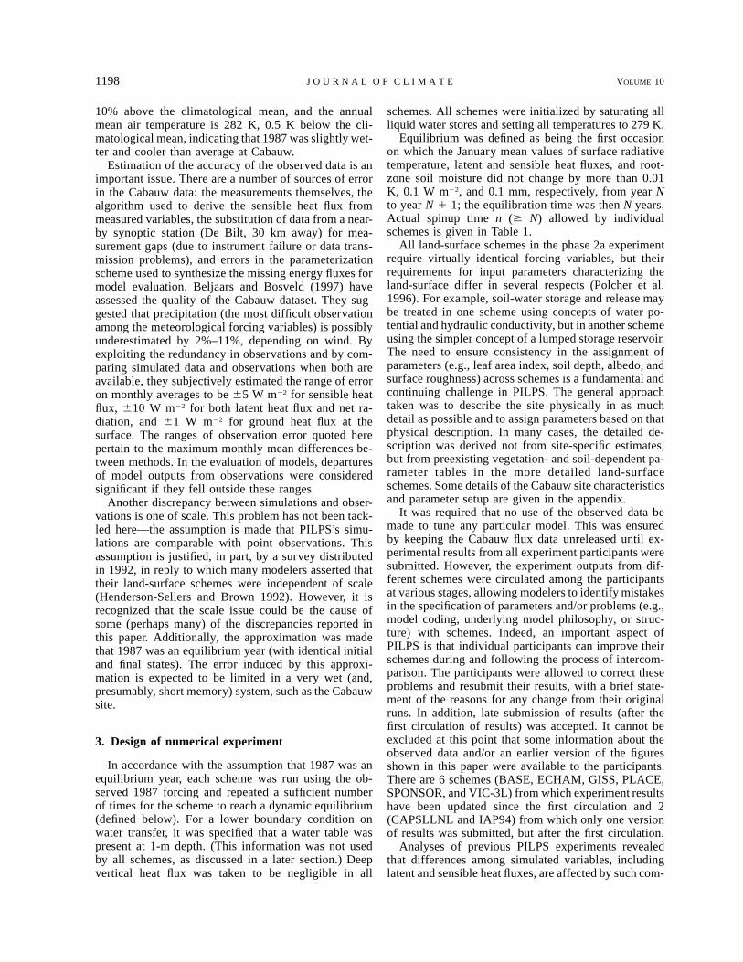
FIG. 2. Annually averaged surface radiative temperature (K).

plications as differing interpretations of instructions andfailures of outputs to satisfy energy balances (Milly etal. 1995; Henderson-Sellers et al. 1995; Love and Hen-derson-Sellers 1995). In phase 2a, it was required thatall results must satisfy a series of tests before beingconsidered in the analysis. For example, outputs fromall schemes were checked to ensure the conservation ofenergy and water over the equilibrium year within thecombined control volume of the soil root zone and thevegetation. Annual means of energy and water fluxesall obeyed

zRn 2 LE 2 Hz , 3 W m22, (1)

where Rn is net radiation, LE is latent heat flux, and His sensible heat flux, and

zP 2 E 2 Y z , 3 mm, (2)

where P is precipitation, E is evapotranspiration, and Yis runoff. Runoff here is defined as the total liquid waterloss from the root-zone–vegetation system by overlandflow, lateral subsurface flow in the root zone, and down-ward flux across the bottom of the root zone; the lastof these terms may be negative because of the presenceof the water table. Ground heat flux is not included in(1) since its annual mean should be zero for the equi-librium year (the annual mean observed ground heatflux is 0.5 W m22). The latent heat of solid–liquid phasechanges does not appear in (1) because of the smallvalue (,1 W m22) of the associated terms. The sameholds for the sensible heat transported by water enteringand leaving the control volume.

4. Results from the Cabauw control simulations

In the PILPS phase 2a experiment, the required outputresults include a full year of daily mean values and 10days (10–19 September) of individual model time stepvalues. The analysis here will mainly be focused onenergy and water budgets and their linkage, using annualmean, seasonal (monthly), and diurnal variations. Toreconstruct a typical diurnal cycle, time step outputshave been averaged across the 10 days. Four schemesdid not resolve the diurnal cycle, either because theyused a 24-h time step (SPONSOR and SWAP) or be-cause they employed forcing that was filtered to removethe diurnal cycle (BUCK and CAPSLLNL). These 4schemes are excluded from the plots of diurnal varia-tions. Three simple statistics to be used throughout thissection are defined as follows: M 5 1/m xi, STDmSi51

5 1/m (xi 2 M)2, and Di 5 xi 2 M, where i ismSÏ i51

a scheme index, m is the number of schemes (23), x isany output variable, M is its mean across schemes, STDis its standard deviation across schemes, and Di is itsdeviation in scheme i from the mean of all schemes.The variable x may represent either a monthly mean ora time step value.

a. Radiation

The surface net radiation is given by

Rn 5 (1 2 a) Rs 1 ∈Rld 2 ∈s ,4Tr (3)

where Rs is shortwave radiation, Rld is downward long-wave radiation, Tr is surface radiative temperature, a issurface albedo, ∈ is thermal emissivity, and s is Stefan–Boltzmann constant. Among the variables and param-eters on the right-hand side of (3), only Tr and a varyacross schemes; the emissivity was assigned a value of1. Furthermore, the effective mean, snow-free value ofalbedo was also prescribed. Given the limited role ofsnow at this site, it was found that Tr was the mainvariable explaining variance of Rn across schemes.

Figure 2 shows the annually averaged surface radi-ative temperature simulated by individual models com-pared with observations. The observed value was de-rived from the measurements of upward and downwardlongwave radiation, Rlu and Rld, for each measurementperiod (30 min)—that is,

Rlu 5 ∈s 1 (1 2 ∈) Rld.4Tr (4)

The observation point in Fig. 2 was obtained using anemissivity of 1, consistent with the specifications forthe model intercomparison; other values of emissivitywere used in (4) for the sensitivity analysis to be de-scribed later. Most models predict a radiative temper-ature between 281 and 282 K, which is above the ob-served value (280.6 K). There is a range of 2 K acrossmodels.


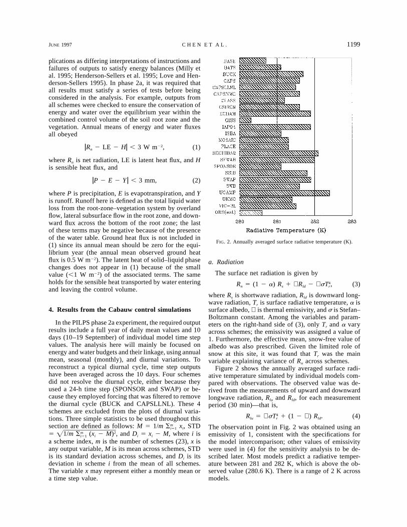
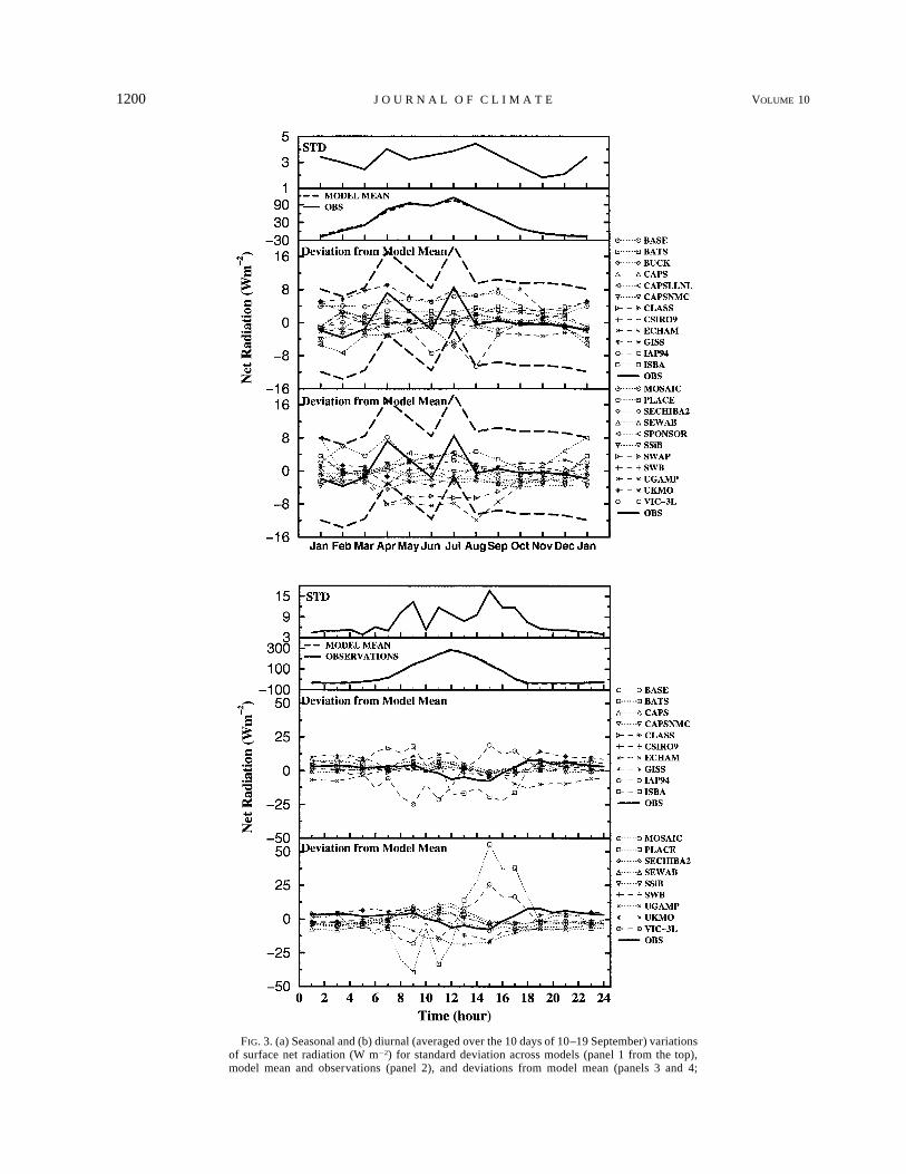
FIG. 3. (a) Seasonal and (b) diurnal (averaged over the 10 days of 10–19 September) variationsof surface net radiation (W m22) for standard deviation across models (panel 1 from the top),model mean and observations (panel 2), and deviations from model mean (panels 3 and 4;

JUNE 1997 1201C H E N E T A L .

←

results are split into two panels for easier identification, and the keys for schemes are listed in alphabetical order). The two thick dashedlines in panels 3 and 4 represent the estimated 610 W m22 observation errors. Four schemes (BUCK, CAPSLLNL, SPONSOR, and SWAP)are excluded from the plots of diurnal variations because they did not resolve diurnal cycle.

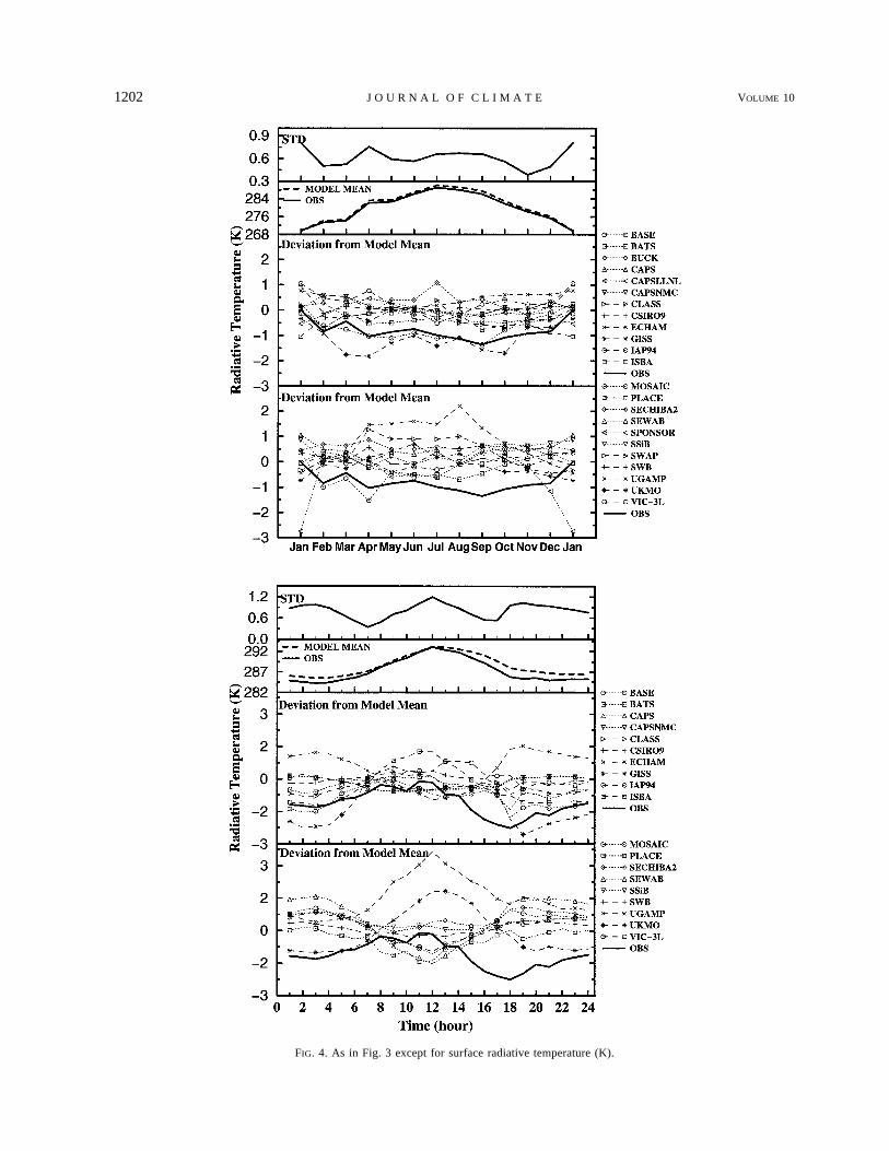
Figure 3 shows the seasonal (Fig. 3a) and diurnal (Fig.3b) variations of surface net radiation by the three sta-tistics. The STD of monthly net radiation has an averageover the year of 3 W m22. The output from each schemedoes not differ from the observation by more than theestimated maximum observation error, except duringApril, May, July, and August, when some schemes sig-nificantly underestimate net radiation. The model meanagrees well with the observations throughout the year,except for April and July. The STD of simulated radi-ative temperature (Fig. 4a) has an average over the yearof 0.6 K. In comparison to the observations, the surfaceradiative temperature is overestimated by most schemesthroughout the year.

At the diurnal scale, the STD of net radiation (Fig.3b) and that of radiative temperature (Fig. 4b) haveaverages over the day of 7 W m22 and 0.8 K, respec-tively. The STD appears to be significantly higher dur-ing the daytime from 0800 to 1800 UTC for net radiationand relatively low around 0700 UTC and 1700 UTC forradiative temperature. The latter is explained by thecharacteristic zero crossings of individual scheme de-viations at these times of day, when the sensible heatflux changes sign. This pattern of intermodel deviationscould be generated by slight to moderate (5%–25%)differences in effective atmospheric bulk transfer co-efficients; such differences are known to exist amongschemes, despite the assignment of fixed roughnesslengths. Another factor is undoubtedly the variability ineffective surface thermal inertia across schemes; thiswill be discussed later in connection with the diurnalenergy fluxes.

Most schemes predict the net radiation with a devi-ation of less than 10 W m22 from the observations. Thediurnal changes in surface radiative temperature simu-lated by most schemes are roughly in agreement withthose observed, but computed values tend to be higherthan observed.

IAP94, ISBA, PLACE, and VIC-3L appear to be theoutliers from the model population of net radiation inFig. 3b. The deviations from model mean are easilyexplained by small phase shifts (on the order of 15 min)of otherwise similar net radiation curves. The evidencesuggests these are an unimportant numerical artifact oftime accounting differences among some schemes. Theydo not appear to be correlated with other anomaliesnoted in the study.

Plots of radiative temperature in Fig. 4a suggest aconsistent model or observational bias, averaging 0.87K across schemes. It is possible that the apparent errorin radiative temperature arises partially from the spec-ification of an emissivity of 1 for the surface. If the

actual emissivity were constant at 0.95, then the meanradiative temperature inferred from observations by (4)would be 0.5 K higher, or 281.1 K. Sensitivity studieswith one model suggest that if an emissivity of 0.95 hadbeen used in the models, computed surface temperaturewould have been only about 0.2 K higher; the lowersensitivity of the models relative to the measurementsis due to the existence of feedbacks in the models, whichcause the longwave irradiance to change as surface tem-perature changes. Extrapolation of these results suggeststhat the bias would vanish at an emissivity of about0.86. Since grassland emissivities are likely to be nosmaller than 0.95 (Sutherland 1986), it appears that onlyabout one-third of the apparent model bias could beremoved if a more realistic emissivity had been used.The discrepancy in radiative temperature could also bedue to the fact that none of the models treats the het-erogeneity of leaf exposure. The highest protruding el-ements are cooled most efficiently and are thus coolerthan the canopy mean, but because of their topmostposition, they contribute a disproportionately large frac-tion of the upward longwave radiation. They are radia-tionally dominant over the warmer, more protected,‘‘average’’ canopy element that most models treat.

b. Latent, sensible, and ground heat fluxes

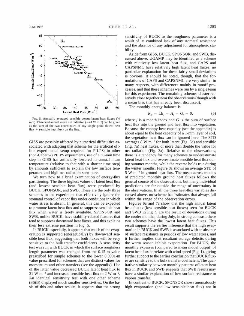
In Fig. 5, the annual mean sensible and latent heatfluxes for various schemes scatter roughly along a linehaving a slope of 21 and intercepts of observed Rn (5H1 LE). Scatter away from the line is associated withdifferences between modeled and observed Rn, which,in turn, are strongly correlated (r 5 20.92) with dif-ferences in annual Tr; the warm bias noted earlier isrelated to the deficit of net radiation in many models.Scatter along the line in Fig. 5 reflects differences inthe surface energy partitioning between latent and sen-sible heat fluxes. The range in annual mean net radiationis just over 10 W m22, and the ranges of sensible andlatent heat fluxes are about 25–30 W m22; differencesin energy flux partitioning, therefore, account for thelarger share of the differences in both heat fluxes.

In fact, a line fitted through the majority of the datapoints in Fig. 5 (excluding outliers GISS and BUCK,discussed below) slopes less than the 1–1 line. This isbecause schemes with low LE have a relative shortageof evaporative cooling, leading to warm surfaces andin turn leading rather directly to low Rn, and hence lowH 1 LE. Results for BUCK apparently depart from thispattern because that scheme did not include stabilityadjustments in its bulk transfer relations; this would tendto produce a warmer surface on average. The results for


FIG. 4. As in Fig. 3 except for surface radiative temperature (K).

JUNE 1997 1203C H E N E T A L .

FIG. 5. Annually averaged sensible versus latent heat fluxes (Wm22). Observed annual mean net radiation (541 W m22) can be givenas the sum of the two coordinates of any single point (latent heatflux 1 sensible heat flux) on the line.

GISS are possibly affected by numerical difficulties as-sociated with adapting that scheme for the artificial off-line experimental setup required for PILPS; in other(non-Cabauw) PILPS experiments, use of a 30-min timestep in GISS has artificially lowered its annual meantemperature (relative to that with a shorter time step)by amounts sufficient to explain the low surface tem-perature and high net radiation seen here.

We turn now to a brief examination of energy-fluxpartitioning. The three highest values of latent heat flux(and lowest sensible heat flux) were produced byBUCK, SPONSOR, and SWB. These are the only threeschemes in the experiment that effectively ignore thestomatal control of vapor flux under conditions in whichwater stress is absent. In general, this can be expectedto promote latent heat flux and to suppress sensible heatflux when water is freely available. SPONSOR andSWB, unlike BUCK, have stability-related features thattend to suppress downward heat fluxes, and this explainstheir less extreme position in Fig. 5.

In BUCK especially, it appears that much of the evap-oration is supported (energetically) by downward sen-sible heat flux, suggesting that both fluxes will be verysensitive to the bulk transfer coefficients. A sensitivitytest was run with BUCK in which the surface roughnesslength parameter was changed from the 0.15-m valueprescribed for simple schemes to the lower 0.0001-mvalue prescribed for schemes that use distinct values formomentum and other transfers (see the appendix). Useof the latter value decreased BUCK latent heat flux to31 W m22 and increased sensible heat flux to 2 W m22.An identical sensitivity test with one other scheme(SSiB) displayed much smaller sensitivities. On the ba-sis of this and other results, it appears that the strong

sensitivity of BUCK to the roughness parameter is aresult of its combined lack of any stomatal resistanceand the absence of any adjustment for atmospheric sta-bility.

Aside from GISS, BUCK, SPONSOR, and SWB, dis-cussed above, UGAMP may be identified as a schemewith relatively low latent heat flux, and CAPS andCAPSNMC have relatively high latent heat fluxes; noparticular explanation for these fairly small deviationsis obvious. It should be noted, though, that the for-mulations of CAPS and CAPSNMC are very similar inmany respects, with differences mainly in runoff pro-cesses, and that these schemes were run by a single teamfor this experiment. The remaining schemes cluster rel-atively close together near the observations (though witha mean bias that has already been discussed).

The monthly energy balance is

Rnj 2 LEj 2 Hj 2 Gj 5 0, (5)

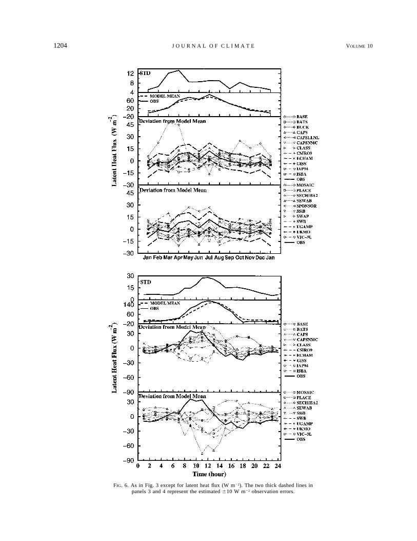
where j is a month index and G is the sum of surfaceheat flux into the ground and heat flux into vegetation.Because the canopy heat capacity (see the appendix) isabout equal to the heat capacity of a 1-mm layer of soil,the vegetation heat flux can be ignored here. The STDaverages 8 W m22 for both latent (Fig. 6a) and sensible(Fig. 7a) heat fluxes, or more than double the value fornet radiation (Fig. 3a). Relative to the observations,there is a tendency for many schemes to underestimatelatent heat flux and overestimate sensible heat flux dur-ing summer months, while the reverse holds true duringthe winter months. Figure 8a shows an average STD of5 W m22 in ground heat flux. The mean across modelsof predicted monthly ground heat fluxes follows thegeneral course of the observations, but many individualpredictions are far outside the range of uncertainty inthe observations. In all the three heat-flux variables dis-cussed above, no scheme has estimates that always fallwithin the range of the observation errors.

Figures 6a and 7a show that the high annual latentheat fluxes (low sensible heat fluxes) seen for BUCKand SWB in Fig. 5 are the result of deviations duringthe cooler months; during July, in strong contrast, thesetwo schemes have the lowest latent heat fluxes. Thisresult supports the earlier inference that the high evap-oration in BUCK and SWB is associated with an absenceof surface resistance in periods of low water stress, andit further implies that resultant storage deficits duringthe warm season inhibit evaporation. For BUCK, themonthly excesses (compared to mean model output) oflatent heat flux correlate with wind speed (Fig. 1), givingfurther support to the earlier conclusion that BUCK flux-es are sensitive to the bulk transfer coefficient. The qual-itative similarity between monthly patterns of latent heatflux in BUCK and SWB suggests that SWB results mayhave a similar explanation of low surface resistance tovapour transfer.

In contrast to BUCK, SPONSOR shows anomalouslyhigh evaporation (and low sensible heat flux) not in


FIG. 6. As in Fig. 3 except for latent heat flux (W m22). The two thick dashed lines inpanels 3 and 4 represent the estimated 610 W m22 observation errors.

JUNE 1997 1205C H E N E T A L .

FIG. 7. As in Fig. 3 except for sensible heat flux (W m22). The two thick dashed lines inpanels 3 and 4 represent the estimated 65 W m22 observation errors.


FIG. 8. As in Fig. 3 except for ground heat flux (W m22). The twothick dashed lines in panels 3 and 4 represent the estimated 61 Wm22 observation errors.

FIG. 9. Averaged rms deviation from monthly observation for sen-sible versus latent heat fluxes (W m22).

winter, but in late spring and early summer. This isconsistent with the fact that SPONSOR neglects sto-matal resistance, but also suppresses downward sensibleheat fluxes. Hence, SPONSOR tends to have unusuallylarge latent heat fluxes only when there is a strong ra-diative energy source (and, of course, an available watersupply). It is not apparent why the SWB pattern ofmonthly latent heat flux is not more like that of SPON-SOR, given the stability adjustments present in SWB.One possibility is that the two stability formulationsused differ significantly in their effects.

Figures 6b, 7b, and 8b illustrate the diurnal cycle ofthe latent, sensible, and ground heat fluxes. The aver-ages, over the day, of STD are 13 W m22 for latent heat

flux, 11 W m22 for sensible heat flux, and 18 W m22

for ground heat flux. The diurnal variation of STD par-allels that of the mean for all three of the heat fluxes,with the highest value around midday (1200 UTC).Compared to the observations, the amplitude of meanmodeled ground heat flux is excessive, its peak is early,and the peak of latent heat flux is late. These discrep-ancies are consistent with those noted by Betts et al.(1993), who attributed them to two deficiencies in theEuropean Centre for Medium-Range Weather Forecastssurface parameterization: insufficient numerical reso-lution of soil temperature near the surface (amplifyingground heat fluxes and delaying turbulent heat fluxes)and delayed transfer of soil temperature information intothe atmospheric boundary layer calculations (causingthe early peak in ground heat flux). The first of theseproblems is a plausible explanation for much of the biasnoted here. Variability in numerical representation ofsoil heat fluxes across schemes is a likely explanationfor the cross-scheme variability in diurnal patterns ofenergy fluxes. We did not attempt to control this aspectof the parameterizations in this experiment, mainly be-cause of the focus on timescales longer than that of thediurnal cycle. This is certainly an area for further at-tention, but it does not appear that the strength of thesedeviations in the diurnal cycle was correlated with anycharacteristics of water or energy fluxes at monthly toannual timescales.

Figure 5 permitted evaluation of the relative accuracyof energy fluxes by schemes, but only on an annualtimescale. As a basis for comparing the quality of en-ergy-flux prediction on a monthly timescale, Fig. 9shows, for each scheme i, the root-mean-square devi-ation ri from observation for monthly heat fluxes:

JUNE 1997 1207C H E N E T A L .

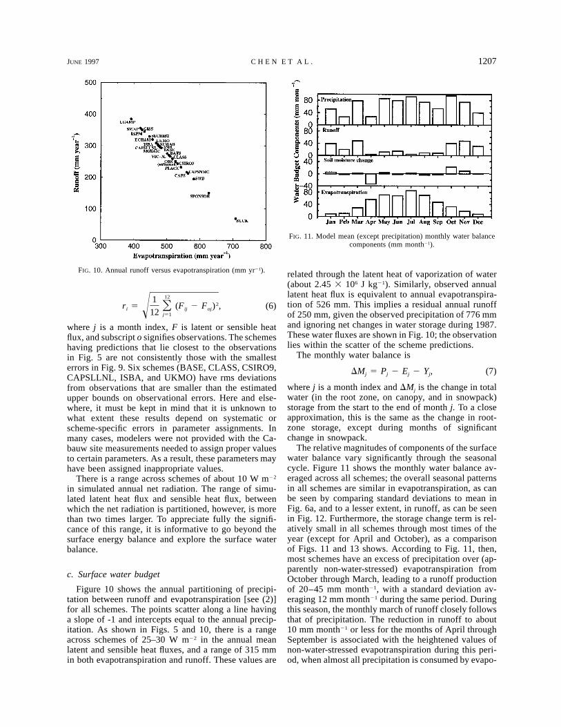
FIG. 10. Annual runoff versus evapotranspiration (mm yr21).

FIG. 11. Model mean (except precipitation) monthly water balancecomponents (mm month21).

1212r 5 (F 2 F ) , (6)Oi ij oj!12 j51

where j is a month index, F is latent or sensible heatflux, and subscript o signifies observations. The schemeshaving predictions that lie closest to the observationsin Fig. 5 are not consistently those with the smallesterrors in Fig. 9. Six schemes (BASE, CLASS, CSIRO9,CAPSLLNL, ISBA, and UKMO) have rms deviationsfrom observations that are smaller than the estimatedupper bounds on observational errors. Here and else-where, it must be kept in mind that it is unknown towhat extent these results depend on systematic orscheme-specific errors in parameter assignments. Inmany cases, modelers were not provided with the Ca-bauw site measurements needed to assign proper valuesto certain parameters. As a result, these parameters mayhave been assigned inappropriate values.

There is a range across schemes of about 10 W m22

in simulated annual net radiation. The range of simu-lated latent heat flux and sensible heat flux, betweenwhich the net radiation is partitioned, however, is morethan two times larger. To appreciate fully the signifi-cance of this range, it is informative to go beyond thesurface energy balance and explore the surface waterbalance.

c. Surface water budget

Figure 10 shows the annual partitioning of precipi-tation between runoff and evapotranspiration [see (2)]for all schemes. The points scatter along a line havinga slope of -1 and intercepts equal to the annual precip-itation. As shown in Figs. 5 and 10, there is a rangeacross schemes of 25–30 W m22 in the annual meanlatent and sensible heat fluxes, and a range of 315 mmin both evapotranspiration and runoff. These values are

related through the latent heat of vaporization of water(about 2.45 3 106 J kg21). Similarly, observed annuallatent heat flux is equivalent to annual evapotranspira-tion of 526 mm. This implies a residual annual runoffof 250 mm, given the observed precipitation of 776 mmand ignoring net changes in water storage during 1987.These water fluxes are shown in Fig. 10; the observationlies within the scatter of the scheme predictions.

The monthly water balance is

DMj 5 Pj 2 Ej 2 Yj, (7)

where j is a month index and DMj is the change in totalwater (in the root zone, on canopy, and in snowpack)storage from the start to the end of month j. To a closeapproximation, this is the same as the change in root-zone storage, except during months of significantchange in snowpack.

The relative magnitudes of components of the surfacewater balance vary significantly through the seasonalcycle. Figure 11 shows the monthly water balance av-eraged across all schemes; the overall seasonal patternsin all schemes are similar in evapotranspiration, as canbe seen by comparing standard deviations to mean inFig. 6a, and to a lesser extent, in runoff, as can be seenin Fig. 12. Furthermore, the storage change term is rel-atively small in all schemes through most times of theyear (except for April and October), as a comparisonof Figs. 11 and 13 shows. According to Fig. 11, then,most schemes have an excess of precipitation over (ap-parently non-water-stressed) evapotranspiration fromOctober through March, leading to a runoff productionof 20–45 mm month21, with a standard deviation av-eraging 12 mm month21 during the same period. Duringthis season, the monthly march of runoff closely followsthat of precipitation. The reduction in runoff to about10 mm month21 or less for the months of April throughSeptember is associated with the heightened values ofnon-water-stressed evapotranspiration during this peri-od, when almost all precipitation is consumed by evapo-


FIG. 12. As in Fig. 3a except for modeled runoff (mm month21).

FIG. 13. As in Fig. 3a except for modeled root-zone (1 m) soil moisture change (mm month21).

JUNE 1997 1209C H E N E T A L .

transpiration. The periods of high and low runoff areseparated by months of significant storage increase inOctober and decrease in April. These seasonal patternsof fluxes and storage changes are consistent with a sim-ple conceptual model (e.g., Milly 1994a,b) having soil-moisture storage near some maximum sustainable value(i.e., ‘‘field capacity’’) in winter, storage depletion inspring, storage below field capacity in summer, and stor-age replenishment in fall.

Beyond the general similarities noted above, theschemes do differ quantitatively in their monthly par-titioning of precipitation into storage change (averageSTD of 11 mm month21), runoff (12 mm month21), andevapotranspiration or latent heat flux (9 mm month21).(For comparison with energy fluxes, 1 mm month21 isapproximately equivalent to 1 W m22.) The largestmonthly STDs (about 20 mm month21) are associatedwith runoff and storage change and occur during themonths of April and October. These are months when,on average across schemes, the runoff season is endingor starting; some variability across schemes in the tim-ing of these seasons could easily explain these maxima.Close examination of Figs. 12 and 13 reveals a signif-icant negative cross correlation between deviations ofrunoff and storage change during April and October.This implies that the variability during these transitionmonths results not so much from variability of non-water-stressed evapotranspiration, but from differencesin model parameterizations of soil water, runoff, andtheir interaction.

Another notable feature seen in Figs. 12 and 13 isthe stronger seasonal cycle of storage and associatedweaker seasonal cycle of runoff for CSIRO9 and VIC-3L, which may be indicative of a stronger propensityof those schemes to produce runoff even in the presenceof a water-storage deficit. This suggestion will be re-visited later in the discussion of modes of runoff andstorage of soil water. The winter runoff deficit in BUCKand the summer runoff deficit in SPONSOR seen in Fig.12 are directly connected to the contemporaneous highvalues of latent heat flux already discussed in connectionwith Fig. 6a.

As discussed earlier, winter (November–March)evapotranspiration is probably not limited by water sup-ply in most schemes. This implies that the variabilityof evapotranspiration during this season is controlledby variability of energy supply, non-water-stressed sur-face resistance to vapor transport, and aerodynamictransport parameterizations across schemes. The result-ing variability of water surplus (precipitation minusevapotranspiration) must be amplified by differences insoil-moisture and runoff parameterizations to producethe somewhat higher variabilities of runoff and storagechanges.

The importance of soil-water stress during summer(May–September) is not clear; it may or may not be afactor in any given scheme. The near equality of pre-cipitation and evapotranspiration is suggestive of pos-

sible water limitation, but the average root-zone soil-water decrease from winter to summer is only about 40mm. The absence of a significant summer peak in thelatent-heat-flux variability supports the hypothesis thateven summer evapotranspiration variability is largelycontrolled by factors other than water availability. Itwould follow that variability of annual mean runoffacross schemes is determined directly by the variabilityin the difference between annual means of precipitationand non-water-stressed evapotranspiration; this is sim-ply the variability in evapotranspiration, because pre-cipitation is constant across schemes. In addition to this,differences in soil-moisture and runoff parameteriza-tions determine the timing of runoff through the year,explaining part of the variance of monthly runoff andstorage change.

It is not surprising that the Cabauw site might ex-perience little water stress throughout the year, giventhe presence of a shallow water table. However, basedon a review of experimental procedures, it appears thatthis water source was ignored in over half of theschemes; most schemes retained their assumption of freegravity drainage of the soil column. This assumption isstandard in schemes designed for use with atmosphericmodels. The apparent rarity of water stress in most mod-els appears to have arisen simply from the near adequacyof the water supply (precipitation and stored soil water)to meet evaporative demands.

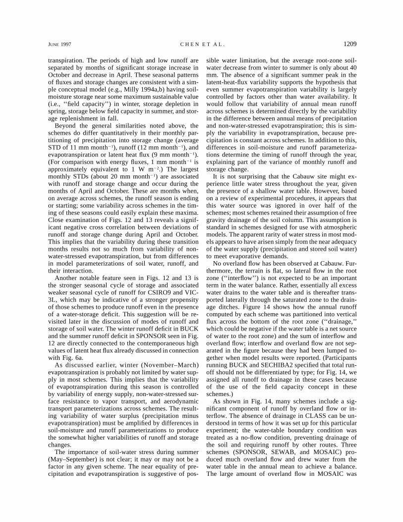
No overland flow has been observed at Cabauw. Fur-thermore, the terrain is flat, so lateral flow in the rootzone (‘‘interflow’’) is not expected to be an importantterm in the water balance. Rather, essentially all excesswater drains to the water table and is thereafter trans-ported laterally through the saturated zone to the drain-age ditches. Figure 14 shows how the annual runoffcomputed by each scheme was partitioned into verticalflux across the bottom of the root zone (‘‘drainage,’’which could be negative if the water table is a net sourceof water to the root zone) and the sum of interflow andoverland flow; interflow and overland flow are not sep-arated in the figure because they had been lumped to-gether when model results were reported. (Participantsrunning BUCK and SECHIBA2 specified that total run-off should not be differentiated by type; for Fig. 14, weassigned all runoff to drainage in these cases becauseof the use of the field capacity concept in theseschemes.)

As shown in Fig. 14, many schemes include a sig-nificant component of runoff by overland flow or in-terflow. The absence of drainage in CLASS can be un-derstood in terms of how it was set up for this particularexperiment; the water-table boundary condition wastreated as a no-flow condition, preventing drainage ofthe soil and requiring runoff by other routes. Threeschemes (SPONSOR, SEWAB, and MOSAIC) pro-duced much overland flow and drew water from thewater table in the annual mean to achieve a balance.The large amount of overland flow in MOSAIC was


FIG. 14. Annual values of total runoff (diagonally hatched bar) andthe sum of overland flow and interflow (solid bar). (Drainage is equalto total runoff minus the sum of overland flow and interflow; it isnegative in MOSAIC, SEWAB, and SPONSOR.) Values are in mmyr21.

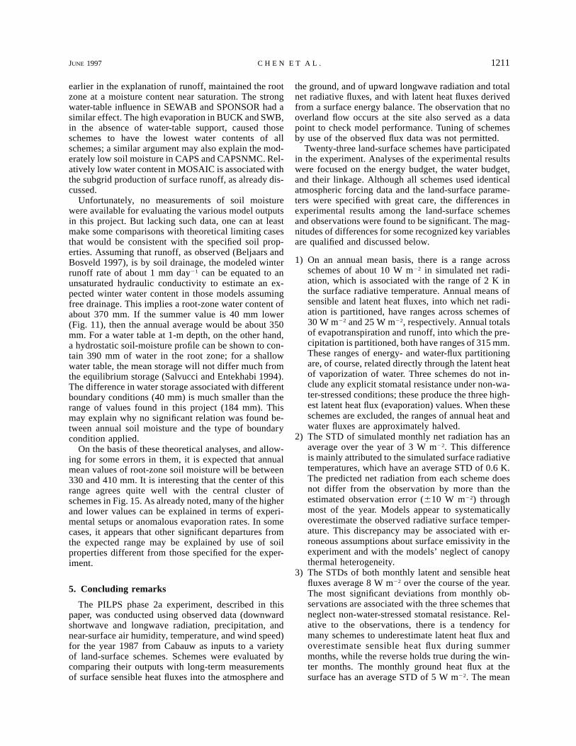
FIG. 15. Annually averaged root-zone (1 m) soil moisture (mm).

caused by a parameterization designed to represent par-tial-area saturation at the subgrid scale of GCMs; it maynot have been appropriate for use at the relatively smalland homogeneous Cabauw site. In contrast, high over-land flow from SPONSOR and SEWAB appears to haveresulted from an excessive influence of the water tableon root-zone water content, which was near saturationat least most of the year in those schemes. High watercontent promotes surface runoff by minimizing the porevolume available to receive infiltration. In the case ofSPONSOR, the cause of this ‘‘waterlogging’’ was a non-physical parameterization of soil water flow, which hassince been replaced. For the remaining four schemes(BATS, CSIRO9, ECHAM, and VIC-3L) having a sig-nificant fraction of runoff by modes other than drainage,the most likely explanation appears to be a propensityfor surface runoff production under nonsaturated root-zone conditions. For CSIRO9 and VIC-3L, this infer-ence is consistent with their anomalous monthly patternsof runoff and water storage, noted already in connectionwith Figs. 12 and 13.

d. Soil moisture

During the planning of the PILPS phase 2a experi-ment, it was anticipated that the high water table at theCabauw site would tend to ‘‘anchor’’ modeled values

of soil moisture and, therefore, to minimize differencesin soil moisture among schemes. However, as shown inFig. 15, there is a range of 184 mm across schemes inthe simulated root-zone soil moisture; this is equivalentto 24% of annual precipitation or 40% of total porevolume. Apparently, the water-table boundary conditiondid little to reduce the spread; as pointed out above, itturns out that at least half of the models were run undera standard assumption of free soil drainage by gravity,which is equivalent to a very deep water table havingno influence on surface conditions.

Analyses were conducted to determine how much ofthe variances of annual soil moisture or energy- andwater-flux partitioning could be explained by the dif-fering boundary conditions. No significant amount ofcross-scheme variance was explained in any of theseanalyses. Nor was soil moisture a significant predictorof flux partitioning. (The latter result can be explainedpartially by the fact that relations between moisture con-tent and fluxes, though qualitatively similar, often differquantitatively across models.) However, in individualcases, it is possible to explain the extreme values ofroot-zone soil moisture with reference either to featuresof the schemes or to how they were set up for the ex-periment. On the basis of a survey of participants, itappears that PLACE is the only scheme that was givena physical boundary condition consistent with a watertable at 1-m depth, and the resulting water content isconsistent with expectations, as the discussion belowwill show. The vertical no-flow condition used inCLASS at the bottom of the modeled soil depth, noted

JUNE 1997 1211C H E N E T A L .

earlier in the explanation of runoff, maintained the rootzone at a moisture content near saturation. The strongwater-table influence in SEWAB and SPONSOR had asimilar effect. The high evaporation in BUCK and SWB,in the absence of water-table support, caused thoseschemes to have the lowest water contents of allschemes; a similar argument may also explain the mod-erately low soil moisture in CAPS and CAPSNMC. Rel-atively low water content in MOSAIC is associated withthe subgrid production of surface runoff, as already dis-cussed.

Unfortunately, no measurements of soil moisturewere available for evaluating the various model outputsin this project. But lacking such data, one can at leastmake some comparisons with theoretical limiting casesthat would be consistent with the specified soil prop-erties. Assuming that runoff, as observed (Beljaars andBosveld 1997), is by soil drainage, the modeled winterrunoff rate of about 1 mm day21 can be equated to anunsaturated hydraulic conductivity to estimate an ex-pected winter water content in those models assumingfree drainage. This implies a root-zone water content ofabout 370 mm. If the summer value is 40 mm lower(Fig. 11), then the annual average would be about 350mm. For a water table at 1-m depth, on the other hand,a hydrostatic soil-moisture profile can be shown to con-tain 390 mm of water in the root zone; for a shallowwater table, the mean storage will not differ much fromthe equilibrium storage (Salvucci and Entekhabi 1994).The difference in water storage associated with differentboundary conditions (40 mm) is much smaller than therange of values found in this project (184 mm). Thismay explain why no significant relation was found be-tween annual soil moisture and the type of boundarycondition applied.

On the basis of these theoretical analyses, and allow-ing for some errors in them, it is expected that annualmean values of root-zone soil moisture will be between330 and 410 mm. It is interesting that the center of thisrange agrees quite well with the central cluster ofschemes in Fig. 15. As already noted, many of the higherand lower values can be explained in terms of experi-mental setups or anomalous evaporation rates. In somecases, it appears that other significant departures fromthe expected range may be explained by use of soilproperties different from those specified for the exper-iment.

5. Concluding remarks

The PILPS phase 2a experiment, described in thispaper, was conducted using observed data (downwardshortwave and longwave radiation, precipitation, andnear-surface air humidity, temperature, and wind speed)for the year 1987 from Cabauw as inputs to a varietyof land-surface schemes. Schemes were evaluated bycomparing their outputs with long-term measurementsof surface sensible heat fluxes into the atmosphere and

the ground, and of upward longwave radiation and totalnet radiative fluxes, and with latent heat fluxes derivedfrom a surface energy balance. The observation that nooverland flow occurs at the site also served as a datapoint to check model performance. Tuning of schemesby use of the observed flux data was not permitted.

Twenty-three land-surface schemes have participatedin the experiment. Analyses of the experimental resultswere focused on the energy budget, the water budget,and their linkage. Although all schemes used identicalatmospheric forcing data and the land-surface parame-ters were specified with great care, the differences inexperimental results among the land-surface schemesand observations were found to be significant. The mag-nitudes of differences for some recognized key variablesare qualified and discussed below.

1) On an annual mean basis, there is a range acrossschemes of about 10 W m22 in simulated net radi-ation, which is associated with the range of 2 K inthe surface radiative temperature. Annual means ofsensible and latent heat fluxes, into which net radi-ation is partitioned, have ranges across schemes of30 W m22 and 25 W m22, respectively. Annual totalsof evapotranspiration and runoff, into which the pre-cipitation is partitioned, both have ranges of 315 mm.These ranges of energy- and water-flux partitioningare, of course, related directly through the latent heatof vaporization of water. Three schemes do not in-clude any explicit stomatal resistance under non-wa-ter-stressed conditions; these produce the three high-est latent heat flux (evaporation) values. When theseschemes are excluded, the ranges of annual heat andwater fluxes are approximately halved.

2) The STD of simulated monthly net radiation has anaverage over the year of 3 W m22. This differenceis mainly attributed to the simulated surface radiativetemperatures, which have an average STD of 0.6 K.The predicted net radiation from each scheme doesnot differ from the observation by more than theestimated observation error (610 W m22) throughmost of the year. Models appear to systematicallyoverestimate the observed radiative surface temper-ature. This discrepancy may be associated with er-roneous assumptions about surface emissivity in theexperiment and with the models’ neglect of canopythermal heterogeneity.

3) The STDs of both monthly latent and sensible heatfluxes average 8 W m22 over the course of the year.The most significant deviations from monthly ob-servations are associated with the three schemes thatneglect non-water-stressed stomatal resistance. Rel-ative to the observations, there is a tendency formany schemes to underestimate latent heat flux andoverestimate sensible heat flux during summermonths, while the reverse holds true during the win-ter months. The monthly ground heat flux at thesurface has an average STD of 5 W m22. The mean


across models of predicted ground heat fluxes fol-lows the general course of the observations, but, inmany cases, individual predictions are far outsidethe estimated range of uncertainty in the observa-tions (61 W m22).

For 6 schemes, root-mean-square deviations ofpredictions from monthly observations are less than5 W m22 for sensible heat flux and 10 W m22 forlatent heat flux, which are the estimated upperbounds on observation errors. However, the extentto which these results depend on systematic orscheme-specific errors in parameter assignments isunknown.

4) To reconstruct a typical diurnal cycle, time step out-puts have been averaged across 10 days (10–19 Sep-tember). Values of STD, defined with respect to10-day mean time step values, average 7 W m22 fornet radiation, 0.8 K for radiative temperature, 13 Wm22 for latent heat flux, 11 W m22 for sensible heatflux, and 18 W m22 for ground heat flux, with thehighest variances around midday (1200 UTC) in allthese variables. Most schemes predict the net radi-ation with a deviation of less than 10 W m22 fromthe observations. The diurnal changes in surface ra-diative temperature simulated by most schemes areroughly in agreement with those observed, but com-puted values tend to be higher than observed, asdiscussed already in connection with the monthlyvalues. During the daytime, there is a distinct phaseshift of modeled latent and ground heat fluxes rel-ative to the observations. In the models there is atendency for latent heat flux to peak late and forground heat flux to peak early. In contrast, the phaseof the mean model output appears correct for sensibleheat flux. Deviations in diurnal patterns of temper-ature and energy fluxes are most likely associatedwith different numerical treatments of soil thermalinertia. These deviations on the diurnal timescale donot appear to be correlated with (nor, in particular,causative of) deviations on longer (e.g., monthly)timescales.

5) Schemes differ in their partitioning of precipitationinto evapotranspiration, storage change, and runoff.Monthly values of STD average 9 mm month21 (8W m22) for evapotranspiration (latent heat flux), 11mm month21 for storage change, and 12 mm month21

for runoff. The variability across schemes of runoffand storage change is largest (about 20 mm month21)during April and October, which are months of tran-sition between high and low (or negligible) runoff.This is largely attributable to the differences in themodel parameterizations of soil water, runoff, andtheir interaction. In winter, when evapotranspirationis not limited by water availability, variance of watersurplus (precipitation minus evapotranspiration) isamplified by differences in soil-moisture and runoffparameterizations.

6) The partitioning of annual runoff into its physical

components was examined. Observational evidenceand site topography suggest that overland flow andinterflow are negligible, leaving vertical drainage tothe water table and subsequent groundwater dis-charge as the main mode of runoff at the site. How-ever, the schemes differ widely in their modes ofrunoff. In some cases, the production of overlandflow can be understood in terms of the details of howa scheme was set up (nonoptimally) for the exper-iment. In several other cases, however, it appears thatschemes have an inherent propensity to produceoverland flow that is inconsistent with the obser-vations. The apparent insensitivity of total runoff toits physical partitioning may be explained by therarity of water stress at the site; in the long run,runoff is the difference between precipitation andnon-water-stressed evapotranspiration.

7) On an annual basis the simulated root-zone soil mois-ture has a range across schemes of 184 mm (40%of total pore volume). No field data were availablefor evaluating modeled soil moisture. However, thisrange of model values did appear to be wider thanwhat could be accounted for theoretically. No con-sistent relation was found between the scatter in thepredicted root-zone soil moisture and that in any ofthe energy- and water-flux variables analyzed in thisstudy. This is not surprising, in view of the largevariety of relations between fluxes and water contentthat is found across models. It implies that the dem-onstration of the ability of a scheme to reproduceobserved water content changes does not necessarilyestablish its ability to reproduce water and energyfluxes. In nearly all cases, however, it was possibleto explain the most extreme values of soil moisturein terms of the particulars of the experimental setupor excessive evapotranspiration.

The discrepancy between simulations and observa-tions could be due to a number of reasons: for example,neglected physical processes in the models, uncertaintyabout important parameter values required by someschemes, lack of detailed descriptions of the specificconditions in Cabauw, lack of atmospheric forcing databefore the year that would allow appropriate spinup, orthe assumption that PILPS’s offline simulations are com-parable with point observations.

In this study, the availability of a full year of observedenergy flux data was a major advantage. The absenceof appropriate runoff and soil moisture data for the studyyear, on the other hand, was a serious shortcoming, es-pecially in view of the spread of results for runoff andwater storage. Furthermore, it would have been usefulto demonstrate from the experimental point of view theaccuracy with which the surface water budget is closed.

The focus of this paper has been on a community-wide intercomparison among models. A detailed anal-ysis of each model is beyond the scope of this study.However, the information given in this paper should

JUNE 1997 1213C H E N E T A L .

TABLE A1. Parameters describing soil properties.

Soil porosity 0.468Saturated hydraulic conductivity (m s21) 3.4341 3 1026

Air-entry suction (mm) 45‘‘B’’ of Clapp and Hornberger (1978) 10.39Ratio of thermal conductivity to that of loam 0.75

serve as a reference for individual modeling groups toexplore their model behaviors in this experiment.

Acknowledgments. PILPS is funded through the Na-tional Oceanic and Atmospheric Administration and TheUniversity of Arizona. T. H. Chen is a research fellowin the Climatic Impacts Centre, funded by the AustralianDepartment of the Environment, Sport, and Territories.We acknowledge the support by the Australian ResearchCouncil. The PILPS team acknowledges the RoyalNetherlands Meteorological Institute for providing theCabauw data, which are the result of a long-term bound-ary layer monitoring program in the Netherlands. Ananonymous reviewer stimulated some of the analysesreported here. This is Climatic Impacts Centre paper95/9.

APPENDIX

Site Characteristics and Parameter Setup

In PILPS phase 2a experiment, a set of parameterswas derived from a variety of sources in an attempt tocharacterize the Cabauw site fully. Where possible,these parameters were obtained from site-specific in-formation. When a parameter was not available fromsite-specific observations, typical values were assignedon the basis of the standard set of parameter in BATS(Dickinson et al. 1993) or the Simple Biosphere Model(Sellers et al. 1986). The parameter values were clas-sified into four groups, as given below.

a. Soil properties

Soil is silty clay with negligible surface slope. Soilphysical characteristics were assumed spatially homo-geneous and temporally invariant. It was assumed thatsoil-water flow can be treated using the single-contin-uum approach common in theoretical soil physics. Soilhydraulic and thermal properties for Cabauw, describedby Beljaars and Bosveld (1997), were not known toPILPS at the time the numerical experiments were de-signed and run. The hydraulic properties were assignedon the basis of a misinterpretation of results of Cosbyet al. (1984), which caused the assigned air-entry suctionand saturated hydraulic conductivities to be scaled byfactors of 0.14 and 2.6, respectively, relative to whatthey would have been if they had been assigned valuescentral to the populations of parameters analyzed byCosby et al. (1984) for silty clay. However, the reportedspread of those populations was so large that the pa-rameters used here are not atypical of a silty clay. Soilthermal properties are assumed to be those specified byBATS for its silty clay soil type. Bare-soil roughnesslength was assigned a value typical for soils. The pa-rameters are listed in Table A1.

With the soil physical parameters above and the ma-tric head at the wilting point of the vegetation (see the

following section), the water content of the root zoneat wilting point is 214 mm.

In models treating the root zone as a single waterstore, the effective water capacity was set to 150 mm,following Manabe (1969). An independent estimate wasobtained by determining, using an approximate analyticsolution of the Richards equation, the amount of evapo-transpiration that could occur, following soil saturation,before gravity-induced drainage caused the water con-tent to drop to the wilting point, given typical non-water-stressed rates of evapotranspiration. (In the context ofa simple storage model, this amount of evaporationwould be identical to the effective water capacity.) Theestimates derived by this approach did not differ bymore than 10–20 mm from the value of 150 mm. Addingthis standard value to the ‘‘unavailable’’ water contentat wilting yields an estimate (364 mm) of root-zone soilmoisture at the free-gravity-drainage field capacity ofthe soil. This is consistent with the estimated winterwater content under free drainage (370 mm) given inthe text.

For models without explicit water-stressed stomatalcontrol of transpiration, the critical water content, abovewhich evapotranspiration equals the non-water-stressed rate, was taken to be 75% of the effective ca-pacity.

b. Vegetation properties

Vegetation is short grass. The root distribution placed70% of the total roots in the top 0.1 m and all remainingroots in the next 0.9 m. The parameters are listed inTable A2.

c. Radiative transfer characteristics

Snow-free albedo of site was specified as being 0.25(Duynkerke 1992) in those models that use albedo as aparameter. Parameters of models with more detailedtreatment were set in an attempt to match an overallalbedo of 0.25. Albedo of fresh snow was taken as being0.75. Other parameters are listed in Table A3.

d. Aerodynamic transfer characteristics

Aerodynamic transfer characteristics were basedmainly on the vegetation structural properties. The mo-mentum roughness length was set to 0.15 m (Beljaarsand Bosveld 1997) and the zero-plane displacementheight to zero. Roughness lengths for heat and moisture


TABLE A2. Parameters describing vegetation properties.

Leaf area indexJan Feb Mar Apr May Jun Jul Aug Sep Oct Nov Dec0.8 1.0 1.1 1.3 1.6 1.8 1.8 1.6 1.5 1.1 1.0 0.9

Fractional vegetation coverJan Feb Mar Apr May Jun Jul Aug Sep Oct Nov Dec0.92 0.93 0.94 0.95 0.97 0.98 0.99 0.98 0.97 0.96 0.95 0.93

Green leaf fractionJan Feb Mar Apr May Jun Jul Aug Sep Oct Nov Dec0.85 0.88 0.89 0.91 0.92 0.93 0.83 0.86 0.67 0.81 0.79 0.77

Maximum height of vegetation (m) 0.2Height of maximum canopy density (m) 0.15Stem area index 4Minimum stomatal resistance (s m21) 40Maximum stomatal resistance (s m21) 20 000Interception capacity (mm) 0.1 3 LAICanopy heat capacity (J m22 K21) 2000Soil-water matric head at wilting (m) 150

TABLE A3. Parameters describing radiative transfer characteristics.

Visible (shortwave) albedo of canopy 0.15Near-infrared (NIR) albedo of canopy 0.35‘‘Visible’’ albedo of fresh snow (.0.7 mm) 0.65NIR albedo of fresh snow (,0.7 mm) 0.85Thermal emissivity of all surface components 1

TABLE A4. Parameters describing aerodynamic transfercharacteristics.

Von Karman constant 0.378Momentum roughness length of bare soil (m) 0.001Momentum roughness length of snow on ground (m) 0.0024

were set equal to that for momentum in some models,but to 0.0001 m (Beljaars and Holtslag 1991) in thosemodels that allow different values. Other parameters arelisted in Table A4.

REFERENCES

Abramopoulos, F., C. Rosenzweig, and B. Choudhury, 1988: Im-proved ground hydrology calculations for global climate models(GCMs): Soil water movement and evapotranspiration. J. Cli-mate, 1, 921–941.

Beljaars, A. C. M., 1982: The derivation of fluxes from profiles inperturbed areas. Bound.-Layer Meteor., 24, 35–55., and A. A. M. Holtslag, 1991: Flux parameterization over landsurfaces for atmospheric models. J. Appl. Meteor., 30, 327–341., and P. Viterbo, 1994: The sensitivity of winter evaporation tothe formulation of aerodynamic resistance in the ECMWF model.Bound.-Layer Meteor., 71, 135–149., and F. C. Bosveld, 1997: Cabauw data for the validation ofland surface parameterization schemes. J. Climate, 10, 1172–1193.

Betts, A. K., J. H. Ball, and A. C. M. Beljaars, 1993: Comparisonbetween the land surface response of the European Centre Modeland the FIFE-1987 data. Quart. J. Roy. Meteor. Soc., 119, 975–1001.

Chen, F., K. Mitchell, J. Schaake, Y. Xue, H.-L. Pan, V. Koren, Q.

Duan, and A. Betts, 1995: Modeling of land-surface evaporationby four schemes and comparison with FIFE observations. J.Geophys. Res., 101, 7251–7268.

Clapp, R. B., and G. M. Hornberger, 1978: Empirical equations forsome soil hydraulic properties. Water Resour. Res., 14, 601–604.

Cosby, B. J., G. M. Hornberger, R. B. Clapp, and T. R. Ginn, 1984:A statistical exploration of the relationships of soil moisturecharacteristics to the physical properties of soils. Water Resour.Res., 20, 682–690.

Dickinson, R. E., A. Henderson-Sellers, P. J. Kennedy, and M. F.Wilson, 1986: Biosphere Atmosphere Transfer Scheme (BATS)for the NCAR Community Climate Model. NCAR Tech. NoteTN2751STR, 69 pp. [Available from National Center for At-mospheric Research, P.O. Box 3000, Boulder, CO 80307.], , and , 1993: Biosphere Atmosphere Transfer Scheme(BATS) Version 1e as coupled to the NCAR Community ClimateModel. NCAR Tech. Note TN3831STR, 72 pp. [Available fromNational Center for Atmospheric Research, P.O. Box 3000, Boul-der, CO 80307.]

Driedonks, A. G. M., H. van Dop, and H. Kohssied, 1978: Meteo-rological observations on the 213 m mast at Cabauw in theNetherlands. Proc. Fourth Symp. Meteorological Observationsand Instruments Denver, CO, Amer. Meteor. Soc., 41–46.

Ducoudre, N. I., K. Laval, and A. Perrier, 1993: SECHIBA, a newset of parameterizations of the hydrologic exchanges at the land–atmosphere interface within the LMD atmospheric general cir-culation model. J. Climate, 6, 248–273.

Dumenil, L., and E. Todini, 1992: A rainfall-runoff scheme for usein the Hamburg climate model. Advances in Theoretical Hy-drology, J. P. O’Kane, Ed., European Geophysical Society Serieson Hydrological Sciences, Vol. 1, Elsevier Science Publishers,129–157.

Duynkerke, P. G., 1992: On the roughness length for heat and othervegetation parameters for a surface of short grass. J. Appl. Me-teor., 31, 579–586.

Goutorbe, J. P., and C. Tarrieu, 1991: HAPEX-MOBILHY data base.Land Surface Evaporation, T. J. Schmugge and J. C. Andre, Eds.,Springer-Verlag, 403–410.

Gregory, D., and R. N. B. Smith, 1994: Canopy, surface and soilhydrology. Unified Model Documentation Paper 25, 19 pp.[Available from U.K. Meteorological Office, London Road,Bracknell, Berkshire RG12 2SZ, United Kingdom.]

Henderson-Sellers, A., and V. B. Brown, 1992: Project for Intercom-parison of Land Surface Parameterization Schemes (PILPS):

JUNE 1997 1215C H E N E T A L .

First science plan. GEWEX Tech. Note, IGPO Publ. Series 5,53 pp., A. J. Pitman, P. K. Love, P. Irannejad, and T. H. Chen, 1995:The Project for Intercomparison of Land-Surface Parameteriza-tion Schemes (PILPS): Phases 2 and 3. Bull. Amer. Meteor. Soc.,76, 489–503.

Holtslag, A. A. M., and A. P. van Ulden, 1983: A simple scheme fordaytime estimates of the surface fluxes from routine weatherdata. J. Climate Appl. Meteor., 22, 517–529.

Kim, J., and M. Ek, 1995: A simulation of the surface energy budgetand soil water content over the Hydrologic Atmospheric PilotExperiments–Modelisation du Bilan Hydrique forest site. J. Geo-phys. Res., 100, 20 845–20 854.

Koster, R. D., and M. J. Suarez, 1992: Modelling the land surfaceboundary in climate models as a composite of independent veg-etation stands. J. Geophys. Res., 97, 2697–2715.

Kowalczyk, E. A., J. R. Garratt, and P. B. Krummel, 1991: A soil-canopy scheme for use in a numerical model of the atmosphere—1D stand-alone model. CSIRO Division of Atmospheric Re-search Tech. Paper 23, 56 pp. [Available from CSIRO Divisionof Atmospheric Research, PMB 1, Aspendale, Vic. 3195, Aus-tralia.]

Liang, X., D. P. Lettenmaier, E. F. Wood, and S. J. Burges, 1994: Asimple hydrologically based model of land surface water andenergy fluxes for general circulation models. J. Geophys. Res.,99 (D7), 415–428., E. F. Wood, and D. P. Lettenmaier, 1996: Surface soil moistureparameterization of the VIC-2L model: Evaluation and modifi-cation. Global Planet. Change, 13, 195–206.

Love, P. K., and A. Henderson-Sellers, 1995: Land surface clima-tologies of AMIP-PILPS models and identification of regionsfor future investigation (PILPS Phase 3a). GEWEX Tech. Note,IGPO Publ. Series 9, 47 pp.

Mahrt, L., and H.-L. Pan, 1984: A two-layer model of soil hydrology.Bound.-Layer Meteor., 29, 1–20.

Manabe, S., 1969: Climate and ocean circulation 1. The atmosphericcirculation and the hydrology of the earth’s surface. Mon. Wea.Rev., 97, 739–774.

Milly, P. C. D., 1994a: Climate, interseasonal storage of soil water,and the annual water balance. Adv. Water Resour., 17, 19–24., 1994b: Climate, soil water storage, and the average annualwater balance. Water Resour. Res., 30, 2143–2156., R. D. Koster, and K. A. Dunne, 1995: Progress in phase 1(c)of the Project for Intercomparison of Land-Surface Parameter-ization Schemes (PILPS). Extended Abstracts, Int. Union of Ge-odesy and Geophysics XXI General Assembly, Boulder, CO,Amer. Geophys. Union, A 190.

Monna, W. A. A., and J. G. van der Vliet, 1987: Facilities for researchand weather observations on the 213-m tower at Cabauw and atremote locations. Scientific Rep. WP-87-5, 27 pp.

Noilhan, J., and S. Planton, 1989: A simple parameterization of landsurface processes for meteorological models. Mon. Wea. Rev.,117, 536–549.

Pan, H.-L., and L. Mahrt, 1987: Interaction between soil hydrology

and boundary layer development. Bound.-Layer Meteor., 38,185–202.

Pitman, A. J., and Coauthors, 1993: Results from the off-line controlsimulation phase of the Project for Intercomparison of Land-Surface Parameterization Schemes (PILPS). GEWEX Tech.Note, IGPO Publ. Series 7, 47 pp.

Polcher, J., K. Laval, L. Dumenil, J. Lean, and P. R. Rowntree, 1996:Comparing three land surface schemes used in GCM. J. Hydrol.,180, 373–394.

Robock, A., K. Ya. Vinnikov, C. A. Schlosser, N. A. Speranskaya,and Y. Xue, 1995: Use of midlatitude soil moisture and mete-orological observations to validate soil moisture simulations withbiosphere and bucket models. J. Climate, 8, 15–35.

Rosenzweig, C., and F. Abramopoulos, 1997: Land-surface modeldevelopment for the GISS GCM. J. Climate, in press.

Salvucci, G. D., and D. Entekhabi, 1994: Equivalent steady soil mois-ture profile and the time compression approximation in waterbalance modeling. Water Resour. Res., 30, 2737–2749.

Schaake, J. C., V. I. Koren, Q. Y. Duan, K. Mitchell, and F. Chen,1995: A simple water balance model (SWB) for estimating runoffat different spatial and temporal scales. J. Geophys. Res., 101,7461–7475.

Sellers, P. J., Y. Mintz, Y. C. Sud, and A. Dalcher, 1986: A SimpleBiosphere Model (SiB) for use within general circulation models.J. Atmos. Sci., 43, 505–531.

Shao, Y., and Coauthors, 1994: Soil moisture simulation, a report ofthe RICE and PILPS workshop. GEWEX Tech. Note, IGPO Publ.Series 14, 179 pp.

Shmakin, A. B., A. Yu. Mikhailov, and S. A. Bulanov, 1993: Param-eterization scheme of the land hydrology considering the orog-raphy at different spatial scales. Exchange Processes at the LandSurface for a Range of Space and Time Scales, H.-J. Bolle, R.A. Feddes, and J. D. Kalma, Eds., IAHS Press, 569–575.

Sutherland, R. A., 1986: Broadband and spectral emissivities (2–18mm) of some natural soils and vegetation. J. Atmos. OceanicTechnol., 3, 199–202.

Verseghy, D. L., 1991: CLASS—A Canadian land surface schemefor GCMs. I. Soil model. Int. J. Climatol., 11, 111–133., N. A. McFarlane, and M. Lazare, 1993: CLASS—A Canadianland surface scheme for GCMs. II: Vegetation model and coupledruns. Int. J. Climatol., 13, 347–370.

Warrilow, D. A., A. B. Sangster, and A. Slingo, 1986: Modelling ofland surface processes and their influence on European climate.Dynamic Climatology Tech. Note 38, 94 pp. [Available fromU.K. Meteorological Office, London Road, Bracknell, BerkshireRG12 2SZ, United Kingdom.]

Wetzel, P. J., and A. Boone, 1995: A Parameterization for Land–Atmosphere–Cloud Exchange (PLACE): Documentation andtesting of a detailed process model of the partly cloudy boundarylayer over heterogeneous land. J. Climate, 8, 1810–1837.

Xue, Y., P. J. Sellers, J. L. Kinter, and J. Shukla, 1991: A simplifiedbiosphere model for climate studies. J. Climate, 4, 345–364.

Yang, Z.-L., R. E. Dickinson, A. Henderson-Sellers, and A. J. Pitman,1995: Preliminary study of spin-up processes in land surfacemodels with the first stage data of Project for Intercomparisonof Land Surface Parameterization Schemes phase 1(a). J. Geo-phys. Res., 100, 16 553–16 578.

Cabauw Experimental Results from the Project for ...

Documents

Transcript of Cabauw Experimental Results from the Project for ...