C2VSim Workshop 3 - C2VSim Land Surface Representation
63
The California Central Valley Groundwater-Surface Water Simulation Model Land Surface Process Charles Brush Modeling Support Branch, Bay-Delta Office California Department of Water Resources, Sacramento, CA CWEMF C2VSim Workshop January 23, 2013
-
Upload
charlie-brush -
Category
Technology
-
view
110 -
download
0
Transcript of C2VSim Workshop 3 - C2VSim Land Surface Representation
The California Central Valley Groundwater-Surface Water
Simulation Model
Land Surface Process
Charles Brush
Modeling Support Branch, Bay-Delta Office
California Department of Water Resources, Sacramento, CA
CWEMF C2VSim WorkshopJanuary 23, 2013

Outline
IWFM Land Surface Process
Land and Water Use Budget
Root Zone Budget
C2VSim Results

IWFM Water Balance Diagram

Land Surface Process

Land Surface Process
PrecipitationEvapotranspiration
Deep Percolation
Diversions
Runoff
Return Flows
Pumping

Land Surface & Root Zone Processes
• Precipitation and irrigation less direct runoff and return flow is the inflow into root zone
• Deep percolation from root zone is the inflow into unsaturated zone
• Net deep percolation from unsaturated zone is the recharge to groundwater
Root Zone
Unsaturated Layer 1
Unsaturated Layer 2
Unsaturated Layer 3
Groundwater
Table
D1
D2
D3
out,1 in,2Q Q
out,2 in,3Q Q
out,3 pQ net D
p in,1D Q
PfI
cadjET
Precipitation
Runoff
Irrigation
AWfI
Return flow
Re-use
• 4 land-use types considered:• agricultural, urban, native • vegetation, riparian vegetation
• Unsaturated zone layer thicknesses are time-dependent; conservation equations in unsaturated zone layers are solved iteratively

Land Surface & Root Zone Processes
• Governing conservation equation for the root zone:
t 1 tr pr r W cadjf
P S A R ET D t
where r = soil moisture, (L);
P = precipitation, (L/T);
Sr = surface runoff from precipitation, (L/T);
AW = applied water, (L/T);
Rf = return flow of applied water, (L/T);
ETcadj = adjusted evapotranspiration, (L/T);
Dp = deep percolation, (L/T);
t = time step length, (T);
t = time step counter (dimensionless).
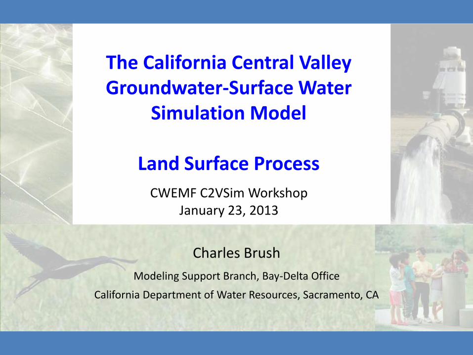
C2VSim Land Surface Process
• 21 Subregions– Annual crop acreages
– Monthly evapotranspiration rates
– Monthly urban demand
– Monthly surface water diversions (Ag & Urban)
– Monthly groundwater pumping (Ag & Urban)
– Regional water re-use factors
• 1392 Elements– Annual land use distribution
– Monthly precipitation

C2VSim Land Surface Process
Input Files:– Precipitation
– Land Use
– Evapotranspiration Rates
– Crop Acreage
– Crop Demands
– Urban Demands
– Urban Specification
– Re-Use Factor
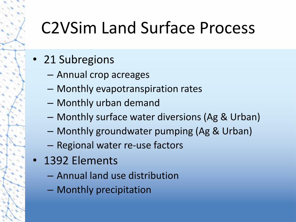
Land Surface & Root Zone Processes
Initial
condition
f
tr

Land Surface & Root Zone Processes
Step 1: Compute rainfall runoff and infiltration of precipitation
• Modified SCS Curve Number method (retention parameter, S,
decreases as moisture goes above half of field capacity)
Runoff
f
Infiltration

Land Surface & Root Zone Processes
Step 2: Apply irrigation and initially assume all infiltrates
Infiltration
f

Land Surface & Root Zone Processes
Step 3: Compute evapotranspiration (FAO Paper 56, 1998)
• Same as potential ET when moisture is at or above half of field
capacity
• Decreases linearly when moisture is below half of field capacity
ETcadj
f

Land Surface & Root Zone Processes
Step 4: Compute deep percolation if moisture is above field capacity
Expressed using one of the methods below specified by user
• A fraction of moisture that is above field capacity
• Physically-based method using hydraulic conductivity;
DP
f
4r
sPT
D K
Land Surface & Root Zone Processes
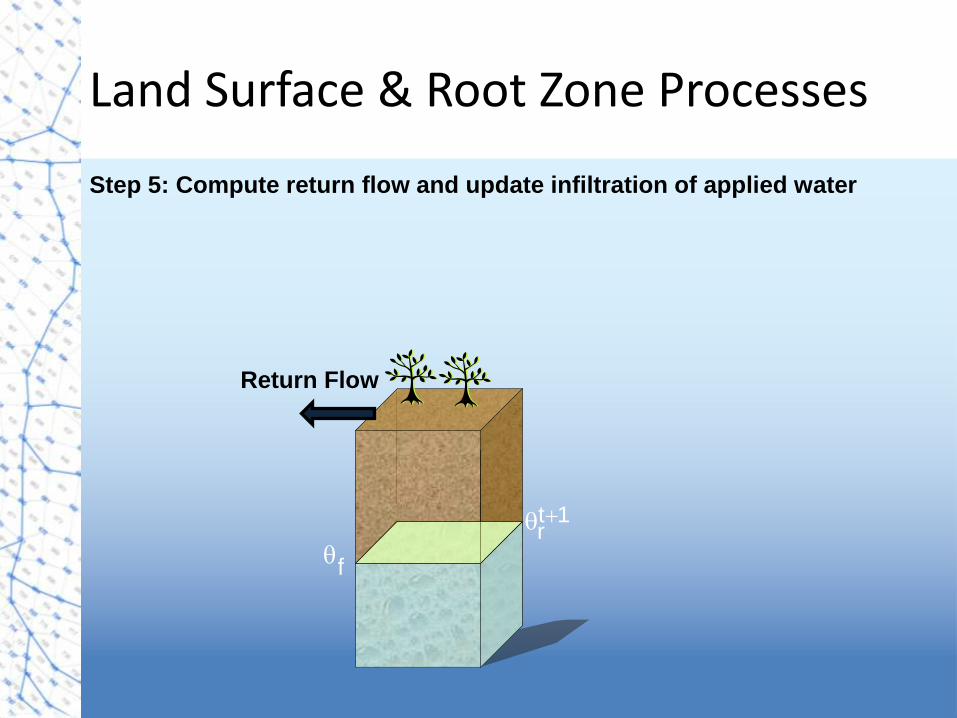
Step 5: Compute return flow and update infiltration of applied water
Return Flow
f
t 1r

Schematic Representation of Flow Components
P = precipitation
Aw = applied water
RP = direct runoff
U = re-use
ET = evapotranspiration
Dr = drain from ponds
D = deep percolation
Rf = net return flow

Soil Moisture Parameters
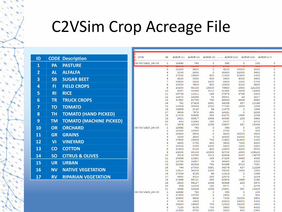
C2VSim Crop Acreage File
ID CODE Description
1 PA PASTURE
2 AL ALFALFA
3 SB SUGAR BEET
4 FI FIELD CROPS
5 RI RICE
6 TR TRUCK CROPS
7 TO TOMATO
8 TH TOMATO (HAND PICKED)
9 TM TOMATO (MACHINE PICKED)
10 OR ORCHARD
11 GR GRAINS
12 VI VINEYARD
13 CO COTTON
14 SO CITRUS & OLIVES
15 UR URBAN
16 NV NATIVE VEGETATION
17 RV RIPARIAN VEGETATION

C2VSim Land Use File

C2VSim Precipitation File

Agricultural Demand Computation
During an irrigation or pre-irrigation period, if the moisture content is below a user-specified threshold, the governing conservation equation is used to compute the value of Aw that will raise the moisture to field capacity:
f ,ini
t 1 tafc
p potfc t t 1min
wR U
t t 1min
P R D ETt if
A 1 f f
0 if
t 1min
t 1fc
t

Evapotranspiration
Assumptions:
• p is taken as 0.5
• ETpot can be
taken as ETc,
ETcadj or
whatever is
specified by the
user
0.00
0.25
0.50
0.75
1.00
0.00 0.25 0.50 0.75 1.00
f f

Crop Demand Varies Monthly
Brush et al. 2005.
Example crop Kc curve
Crop ET = Kc * ETo

C2VSim ETc File
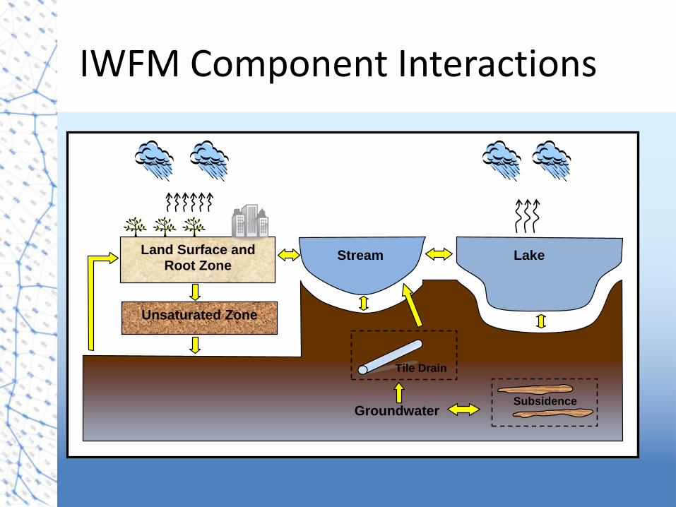
IWFM Component Interactions
Land Surface and Root Zone
Unsaturated Zone
Stream Lake
Groundwater
Tile Drain
Subsidence
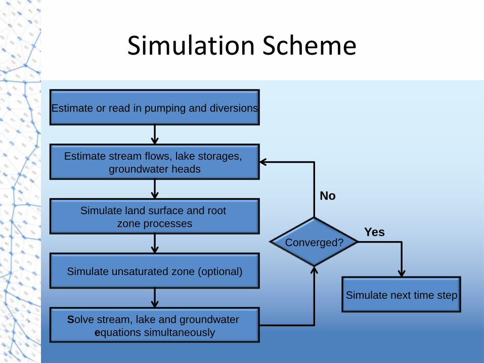
Simulation Scheme
Estimate or read in pumping and diversions
Estimate stream flows, lake storages,
groundwater heads
Simulate land surface and root
zone processes
Simulate unsaturated zone (optional)
Solve stream, lake and groundwater
equations simultaneously
Converged?
No
Yes
Simulate next time step

A Need for Demand Computation
• Routing of water through a developed basin requires the knowledge of applied water
• In California, groundwater pumping is generally neither measured nor regulated; i.e. total historical applied water is unknown
• Most major surface diversions are measured in California’s Central Valley but their spatial allocation may be unknown
• For planning studies applied water is an unknown and has to be computed dynamically
• To address the uncertainties in historical and future water supplies and where these supplies were/will be used, a demand-supply balance is needed
t 1 tr pr r W cadjf
P S A R ET D t

Agricultural Demand Computation
• Agricultural demand is the required amount of applied water in order to maintain optimum agricultural conditions
• At optimum agricultural conditions
1) ET rates are at their potential levels for proper crop growth
Soil moisture interval at which
(i) ET = ETc,
(ii) Dp = 0,
(iii) min
f
f0.5
min
2) soil moisture loss as deep percolation and return flow is minimized
3) minimum soil moisture requirement for each crop is met at all times
Agricultural Demand Computation
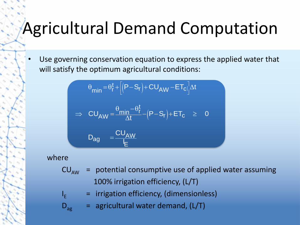
• Use governing conservation equation to express the applied water that will satisfy the optimum agricultural conditions:
tr cr AWmin
trmin
r cAW
AWag
E
P S CU ET t
CU P S ET 0t
CUD
I
where
CUAW = potential consumptive use of applied water assuming
100% irrigation efficiency, (L/T)
IE = irrigation efficiency, (dimensionless)
Dag = agricultural water demand, (L/T)

C2VSim Crop Demands File

Urban Demand & Moisture Routing
• Urban water demands are user-specified time-series input data
• Outdoor urban applied water and precipitation are routed through the root zone using the governing conservation equation
Urban indoor water
Urban outdoor water
• Urban indoor applied water and precipitation over non-pervious urban areas become entirely return flow and surface runoff

Urban Water Use Parameters

C2VSim Urban Specifications File

C2VSim Urban Demands File

Automated Supply Adjustment
• Automatic adjustment of diversions and pumping to meet agricultural and urban water demands
• Diversion or pumping adjustment can be turned on or off during simulation period (represents evolution of water supply facilities over time)
• All supplies have equal priorities; handling of complex water rights is deferred to systems models like CalSim
Agriculture
Urban
Divag
Divurb Purb
Pag
• Useful in estimating historical pumping in Central Valley, and future diversions and pumping
• No supply adjustment for native and riparian vegetation

Balance between Supply and Demand
• IWFM can route water supplies (diversions and pumping) as specified or automatically adjust supplies to meet demands (increase/decrease in diversions and/or pumping)
• When supplies are adjusted, they may still be less than demand if there is not enough water in the system
• When supply is less than demand deep percolation, return flows, moisture content and ET diminish; when larger than demand deep percolation, return flow and moisture content increase

IWFM Output
• Land and Water Use Budget
– Agricultural supply and demand
– Urban supply and demand
– Surface water imports and exports
• Root Zone Moisture Budget
– Agricultural, Urban, Native/Riparian sections
– Land surface water balance for each
– Root zone moisture balance for each

Land and Water Use Budget
• Balance Water Supply and Demand
• Agricultural and Urban Sections
• Calculated for each Subregion
• Agricultural Supply Requirement = Potential CUAW/Irrigation Efficiency
• Urban Supply Requirement is input time series
• Supply Requirement = Pumping + Diversions + Shortage

Land and Water Use Budget

Land and Water Use Budget
Column Flow 08/31/2004 SourceA
gric
ult
ura
l
Area (AC) 6,604,404
Potential CUAW 2,586,635
Supply Requirement OUT 3,294,699
Pumping IN 1,601,200 GW
Diversion IN 1,693,677 SW
Shortage (IN) -177
Re-use 67,228
Urb
an
Area (AC) 1,147,412
Supply Requirement OUT 249,902
Pumping IN 162,716 GW
Diversion IN 91,371 SW
Shortage (IN) -4,185
Re-use 0
Import 949,507
Export 369,919

Land Use Change

42
Land Use Change

Subregion Land Use

Crop Acreage

Sources and Sinks

Sources and Sinks

Agricultural Budget
2000-2009

Urban Budget
2000-2009

Native & Riparian Budget
2000-2009

Ag and Urban Water Use

Agricultural Water Sources
Root Zone Moisture Budget
• Agricultural, Urban and Native/Riparian
• Water Sources and Root Zone sections
• Printed for each Subregion
• Water sources:– All have precipitation
– Agricultural and Urban have applied water
• Root zone– Soil moisture storage +/- land expansion
– Beginning storage + infiltration – ET – deep percolation = ending storage

Root Zone Moisture Budget

Root Zone Moisture Budget
Column Flow 08/31/2004 Process
Agr
icu
ltu
ral
Area (AC) 6,604,404
Precipitation IN 92
Runoff OUT 0 SW
Prime Applied Water 3,294,876
Reused Water 67,228
Total Applied Water IN 3,362,104 GW/SW
Return Flow OUT 99,094 SW
Beginning Storage 4,100,673
Net Gain from Land Expansion (+) +/- 0
Infiltration (+) IN 3,195,874
Actual ET (-) OUT 3,051,486
Deep Percolation (-) OUT 166,381 GW
Ending Storage (=) 4,078,680

Root Zone Moisture Budget
Column Flow 08/31/2004 Process
Urb
an
Area (AC) 1,147,412
Precipitation IN 208
Runoff OUT 79 SW
Prime Applied Water 254,086
Reused Water 0
Total Applied Water IN 254,086 GW/SW
Return Flow OUT 46,801 SW
Beginning Storage 0
Net Gain from Land Expansion (+) +/- 0
Infiltration (+) 207,414
Actual ET (-) 152,581
Deep Percolation (-) 54,833 GW
Ending Storage (=) 0
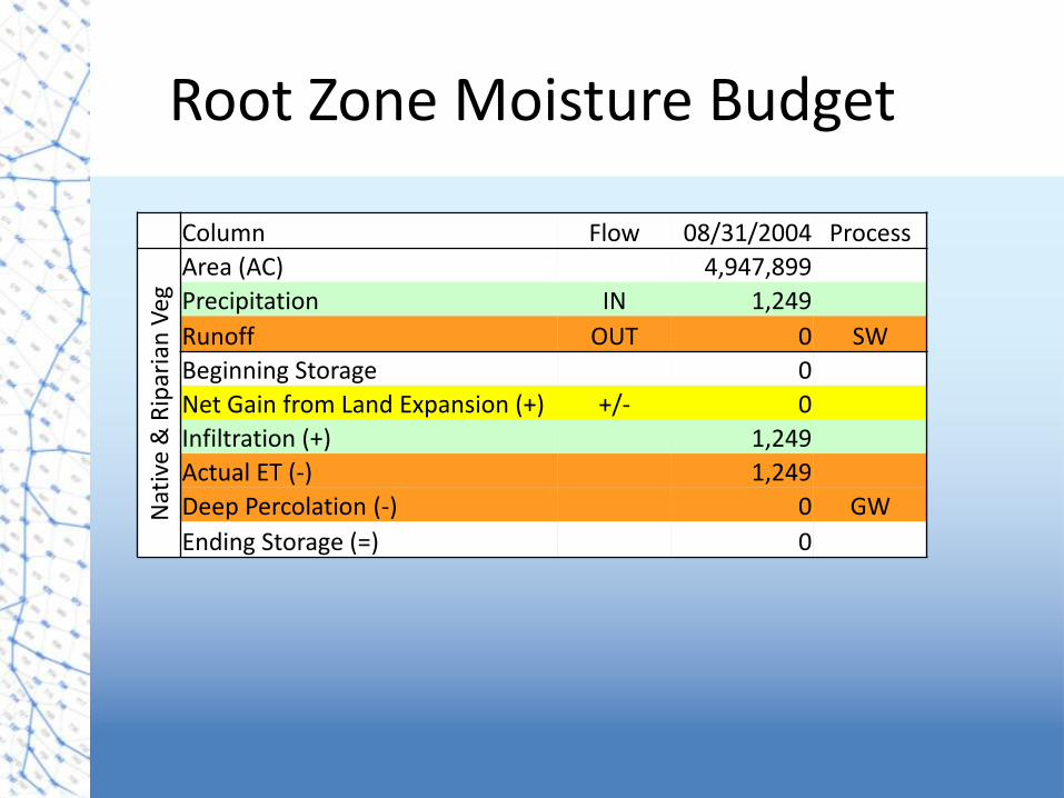
Root Zone Moisture Budget
Column Flow 08/31/2004 Process
Nat
ive
& R
ipar
ian
Veg
Area (AC) 4,947,899
Precipitation IN 1,249
Runoff OUT 0 SW
Beginning Storage 0
Net Gain from Land Expansion (+) +/- 0
Infiltration (+) 1,249
Actual ET (-) 1,249
Deep Percolation (-) 0 GW
Ending Storage (=) 0

Annual Evapotranspiration

Regional ET Distribution

Regional ET Distribution
32%
6%
5%19%
38%
Sacramento Valley
Eastside Sterams
Sacramento-San Joaquin Delta
San Joaquin River Basin
Tulare Basin
2000-2009

Monthly Evapotranspiration

Deep Percolation by Land Use

Summary
• IWFM Land and Water Use Process
– Known inflows: Surface Water Diversions
– Estimated outflows: Evapotranspiration
– Calculated inflows: Groundwater Pumping
• Constrained by water balance between inter-process flows

End