C10.1b { { 16HT Brownian Motion in Complex...

C10.1b – – 16HT

Brownian Motion in Complex Analysis

Dr T CassThe Mathematical Institute,

University of Oxford24-29 St Giles’

Oxford OX1 [email protected]

HT 2009

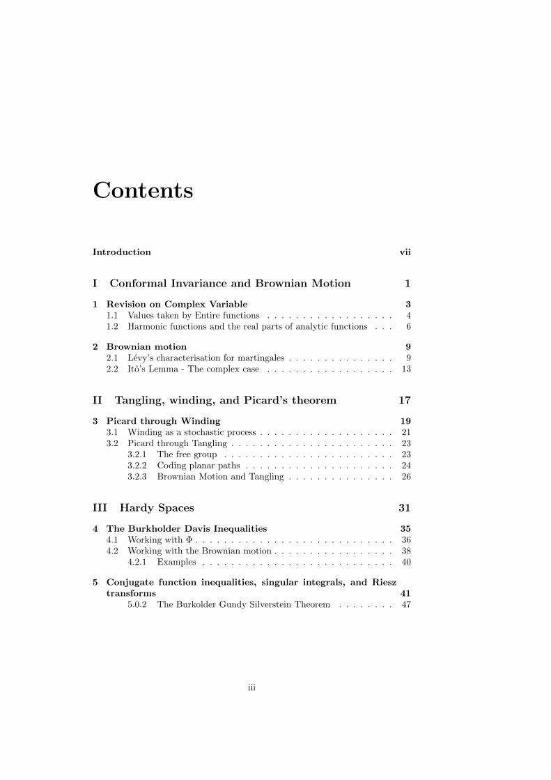
Contents

Introduction vii

I Conformal Invariance and Brownian Motion 1

1 Revision on Complex Variable 31.1 Values taken by Entire functions . . . . . . . . . . . . . . . . . . 41.2 Harmonic functions and the real parts of analytic functions . . . 6

2 Brownian motion 92.1 Levy’s characterisation for martingales . . . . . . . . . . . . . . . 92.2 Ito’s Lemma - The complex case . . . . . . . . . . . . . . . . . . 13

II Tangling, winding, and Picard’s theorem 17

3 Picard through Winding 193.1 Winding as a stochastic process . . . . . . . . . . . . . . . . . . . 213.2 Picard through Tangling . . . . . . . . . . . . . . . . . . . . . . . 23

3.2.1 The free group . . . . . . . . . . . . . . . . . . . . . . . . 233.2.2 Coding planar paths . . . . . . . . . . . . . . . . . . . . . 243.2.3 Brownian Motion and Tangling . . . . . . . . . . . . . . . 26

III Hardy Spaces 31

4 The Burkholder Davis Inequalities 354.1 Working with Φ . . . . . . . . . . . . . . . . . . . . . . . . . . . . 364.2 Working with the Brownian motion . . . . . . . . . . . . . . . . . 38

4.2.1 Examples . . . . . . . . . . . . . . . . . . . . . . . . . . . 40

5 Conjugate function inequalities, singular integrals, and Riesztransforms 41

5.0.2 The Burkolder Gundy Silverstein Theorem . . . . . . . . 47

iii

iv CONTENTS

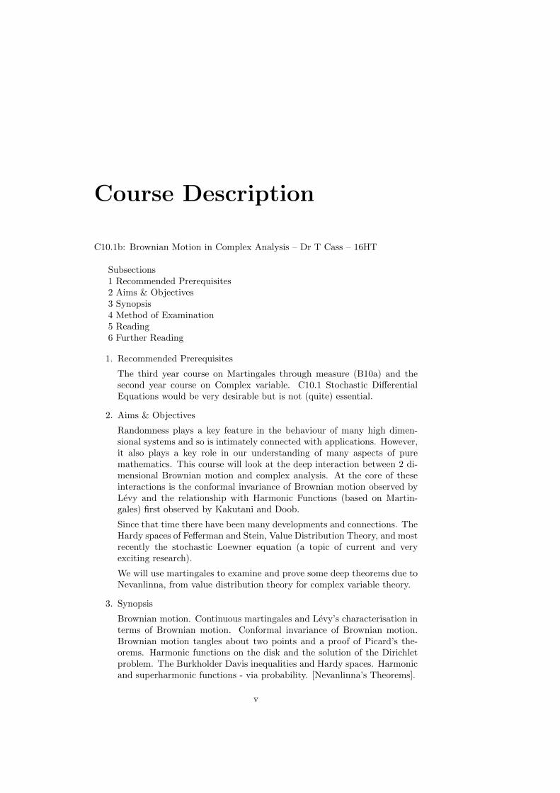
Course Description

C10.1b: Brownian Motion in Complex Analysis – Dr T Cass – 16HT

Subsections1 Recommended Prerequisites2 Aims & Objectives3 Synopsis4 Method of Examination5 Reading6 Further Reading

1. Recommended Prerequisites

The third year course on Martingales through measure (B10a) and thesecond year course on Complex variable. C10.1 Stochastic DifferentialEquations would be very desirable but is not (quite) essential.

2. Aims & Objectives

Randomness plays a key feature in the behaviour of many high dimen-sional systems and so is intimately connected with applications. However,it also plays a key role in our understanding of many aspects of puremathematics. This course will look at the deep interaction between 2 di-mensional Brownian motion and complex analysis. At the core of theseinteractions is the conformal invariance of Brownian motion observed byLevy and the relationship with Harmonic Functions (based on Martin-gales) first observed by Kakutani and Doob.

Since that time there have been many developments and connections. TheHardy spaces of Fefferman and Stein, Value Distribution Theory, and mostrecently the stochastic Loewner equation (a topic of current and veryexciting research).

We will use martingales to examine and prove some deep theorems due toNevanlinna, from value distribution theory for complex variable theory.

3. Synopsis

Brownian motion. Continuous martingales and Levy’s characterisation interms of Brownian motion. Conformal invariance of Brownian motion.Brownian motion tangles about two points and a proof of Picard’s the-orems. Harmonic functions on the disk and the solution of the Dirichletproblem. The Burkholder Davis inequalities and Hardy spaces. Harmonicand superharmonic functions - via probability. [Nevanlinna’s Theorems].

v

vi PREFACE

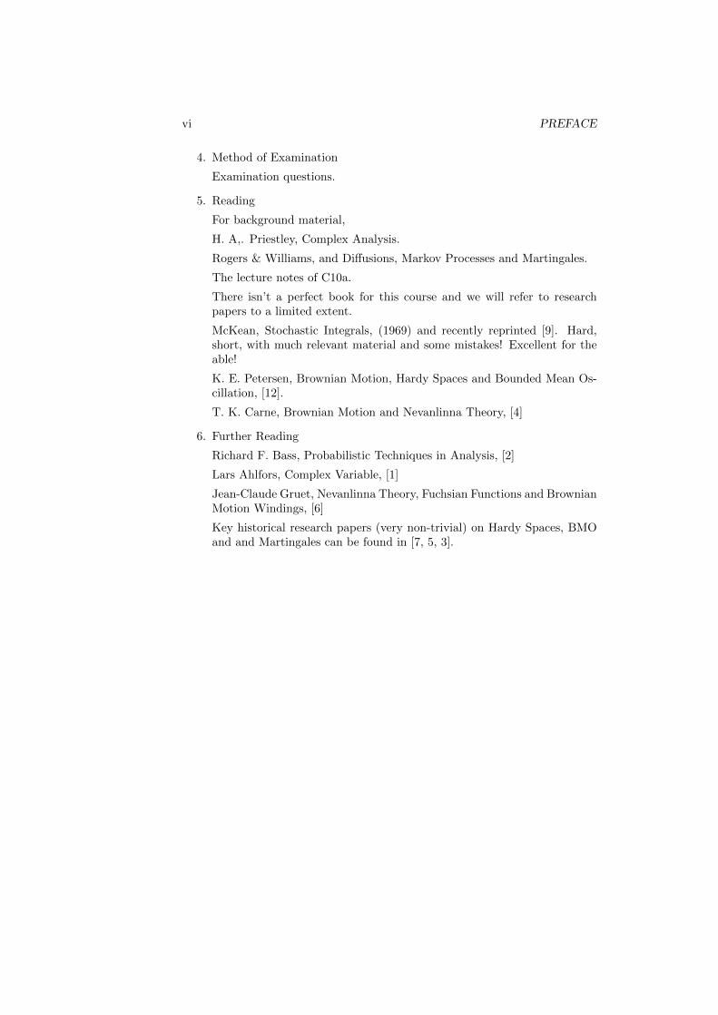
4. Method of Examination

Examination questions.

5. Reading

For background material,

H. A,. Priestley, Complex Analysis.

Rogers & Williams, and Diffusions, Markov Processes and Martingales.

The lecture notes of C10a.

There isn’t a perfect book for this course and we will refer to researchpapers to a limited extent.

McKean, Stochastic Integrals, (1969) and recently reprinted [9]. Hard,short, with much relevant material and some mistakes! Excellent for theable!

K. E. Petersen, Brownian Motion, Hardy Spaces and Bounded Mean Os-cillation, [12].

T. K. Carne, Brownian Motion and Nevanlinna Theory, [4]

6. Further Reading

Richard F. Bass, Probabilistic Techniques in Analysis, [2]

Lars Ahlfors, Complex Variable, [1]

Jean-Claude Gruet, Nevanlinna Theory, Fuchsian Functions and BrownianMotion Windings, [6]

Key historical research papers (very non-trivial) on Hardy Spaces, BMOand and Martingales can be found in [7, 5, 3].

Introduction

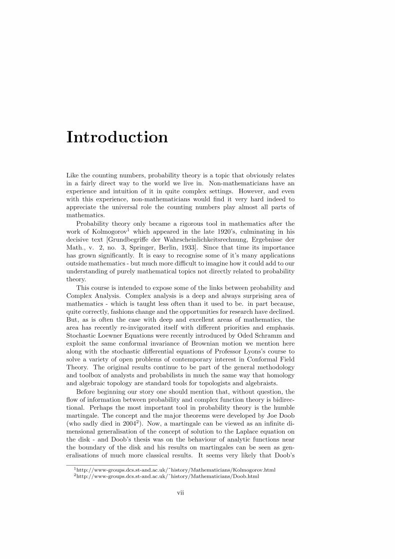
Like the counting numbers, probability theory is a topic that obviously relatesin a fairly direct way to the world we live in. Non-mathematicians have anexperience and intuition of it in quite complex settings. However, and evenwith this experience, non-mathematicians would find it very hard indeed toappreciate the universal role the counting numbers play almost all parts ofmathematics.

Probability theory only became a rigorous tool in mathematics after thework of Kolmogorov1 which appeared in the late 1920’s, culminating in hisdecisive text [Grundbegriffe der Wahrscheinlichkeitsrechnung, Ergebnisse derMath., v. 2, no. 3, Springer, Berlin, 1933]. Since that time its importancehas grown significantly. It is easy to recognise some of it’s many applicationsoutside mathematics - but much more difficult to imagine how it could add to ourunderstanding of purely mathematical topics not directly related to probabilitytheory.

This course is intended to expose some of the links between probability andComplex Analysis. Complex analysis is a deep and always surprising area ofmathematics - which is taught less often than it used to be. in part because,quite correctly, fashions change and the opportunities for research have declined.But, as is often the case with deep and excellent areas of mathematics, thearea has recently re-invigorated itself with different priorities and emphasis.Stochastic Loewner Equations were recently introduced by Oded Schramm andexploit the same conformal invariance of Brownian motion we mention herealong with the stochastic differential equations of Professor Lyons’s course tosolve a variety of open problems of contemporary interest in Conformal FieldTheory. The original results continue to be part of the general methodologyand toolbox of analysts and probabilists in much the same way that homologyand algebraic topology are standard tools for topologists and algebraists.

Before beginning our story one should mention that, without question, theflow of information between probability and complex function theory is bidirec-tional. Perhaps the most important tool in probability theory is the humblemartingale. The concept and the major theorems were developed by Joe Doob(who sadly died in 20042). Now, a martingale can be viewed as an infinite di-mensional generalisation of the concept of solution to the Laplace equation onthe disk - and Doob’s thesis was on the behaviour of analytic functions nearthe boundary of the disk and his results on martingales can be seen as gen-eralisations of much more classical results. It seems very likely that Doob’s

1http://www-groups.dcs.st-and.ac.uk/˜history/Mathematicians/Kolmogorov.html2http://www-groups.dcs.st-and.ac.uk/˜history/Mathematicians/Doob.html

vii

viii INTRODUCTION

understanding of complex function theory - together with an exposure to prob-ability because he was working in a statistics department (because no majormath department offered him a job (he was Jewish)) lead to the developmentof martingales as we know them today.

Part I

Conformal Invariance andBrownian Motion

1

Chapter 1

Revision on ComplexVariable

The complex plane C comprises the algebra of points z = x+ iy, where x and yare real numbers and i2 = −1. The smooth functions f (z) = u (x, y) + iv (x, y)mapping C to C can be identified with smooth function from R2 → R2.Withinthe class of smooth functions, polynomials

∑Nn=0 anz

n form a special subclass.

Definition 1 We say that a function f : D → C defined on an open subset Dof C and given by f = u+ iv with u, v : R2 → R2 is analytic on D if it satisfiesthe Cauchy Riemann equations1

∂f

∂x+ i

∂f

∂y=∂u

∂x− ∂v

∂y+ i

(∂u

∂y+∂v

∂x

)= 0

everywhere on D.

The class of analytic funtions is closed under composition and addition, andso, since f (z) = z is clearly analytic, polynomials are in this class. In generalthese functions f are quite remarkable; they are smooth; infinitely differentiablein the complex sense; and have an exact local power series representations. Themost remarkable results include Cauchy’s theorem, the integral representationformula, Rouche’s theorem and its connection with winding numbers.

Definition 2 A open subset X of a topological space Y is said to be disconnectedif there exist open subsets U and V of Y such that U ∩ V = ∅ and U ∪ V = X.If X is not disconnected we say it is connected.

Recall that continuous, integer valued functions defined on a connected setare constant.

Definition 3 A domain is an open, connected subset of C.

Definition 4 A curve γ : [a, b] → C is said to be closed or is called a loop ifγ (a) = γ (b)

1The notation z = x + iy = (x, y) and f(z) = f(x, y) = u(x, y) + iv(x, y) will allow us to

transfer between C and R2. ∂f∂x

and ∂f∂y

then refer to partial deriatives of f taking values in

R2. See Priestly, Section 1.10 and Theorem 5.3.

3

4 CHAPTER 1. REVISION ON COMPLEX VARIABLE

If γ : [a, b]→ C is a (continuously differentiable) curve which does not passthrough 0 ∈ C, a continuous choice of the argument on γ is a continuous mapθ : [a, b]→ R such that γ (t) = |γ (t)| eiθ(t). The quantity θ (b)− θ (a) measuresthe angle turned through by γ.

Definition 5 We call (θ (b)− θ (a)) /2π the winding number Γ (γ, 0) of γ about0, and we may define Γ (γ,w) for w ∈ C similarly.

One can check that this definition is well defined by taking another continuouschoice of the argument φ and observing that θ (t)− φ (t) is an integer multipleof 2π.Then, the continuous function (θ − φ) /2π is integer valued and since [a, b]is connected it must be constant giving θ (b) − θ (a) = φ (b) − φ (a). If γ isa closed curve then Γ (γ,w) is integer valued and we can describe it using anintegral representation formula (see chapter 3). We call a closed curve γ : [a, b]→ D ⊆ C simple if it does not cross itself, i.e. γ (s) = γ (t) for s and t distinct ifand only if s and t are the endpoints a and b. A contractible loop is one whichcan be continuously deformed to a constant loop.

Theorem 6 (Taylor’s Theorem) If D is a domain, γ is a simple closed curvethat is contractible in D, winding around z once, and f is an analytic functiondefined on D then2

f (z) =1

2πi

∫γ

f (γ)

γ − zdγ

f (n) (z) =n!

2πi

∫γ

f (γ)

(γ − z)n+1 dγ

1.1 Values taken by Entire functions

Definition 7 We say an analytic function f (z) defined on the whole of C isan entire function.

One of our analytical objectives is to study the range of an entire function.This branch of complex analysis is known as Nevanlinna theory, after the Finnishmathematician Rolf Nevanlinna. We can find some easy results in complexanalysis as follows but, as we will see in later sections, much more is true.

Corollary 8 If f is an entire function and |f (z)| < M <∞ for all z ∈ C thenf is constant.

Proof. Suppose that |f (z)| < M on |z| ≤ R then, putting γ (t) = Re2πit, onehas for |z| < R that

f (n) (z) =n!

2πi

∫γ

f (γ)

(γ − z)n+1 dγ

= n!

∫ 1

0

f(Re2πit

)Re2πit

(Re2πit − z)n+1 dt

2The notation∫γ f(γ)dγ refers to

∫ 1t=0 f(γ(t))γ(t) where γ : [0, 1] → C. This (standard)

notation will not cause us confusion. See Priestley, Section 10.3.

1.1. VALUES TAKEN BY ENTIRE FUNCTIONS 5

and

|f ′ (z0)| ≤ MR

|R− r|2

for |z0| < r. Applying the mean value theorem we have

|f (z0)− f (z1)| ≤ MR

|R− r|2|z0 − z1|

≤ 2MRr

|R− r|2

if for |z1| < r as well. If f is entire then we can let R → ∞ and conclude thatf is constant.

The quantitative estimates we derived in the proof are of independent inter-est. For example (as you would see in the functional analysis course C4a), wecould also conclude that any family of analytic functions on a common domainwith a common bound are equicontinuous. By the Stone-Weierstrass and thenArzela-Ascoli theorems the restrictions of these functions to a compact set Kwill always be relatively compact in the uniform norm as a subset of C (K).

So we have seen that an entire function that is not constant must take manyvalues (it cannot be bounded). However, the most obvious entire functions arepolynomials. We have the famous

Theorem 9 (Fundamental Theorem of Algebra) If P (z) is a polynomialof degree d then

P (z) = w

has exactly d complex solutions (when multiplicity is taken into account).

Proof. It is enough to treat the case where P is monic and w = 0 so that

P (z) = zd + ad−1zd−1 + . . .+ a0.

Let γ (t) = Re2πit then using either a simple application of the Residue Theoremor by applying the Argument Principle it follows that the number of zeros insidethe disk |z| = R is given by

1

2πi

∫γ

P ′ (γ)

P (γ)dγ, (1.1)

provided there is no zero of P on the curve γ. Choose

R > 1 + dmax ai|i = 0, . . . , d− 1 .

Now, if |z| > 1 then

|P (z)| > |z|d − dmax |ai||i = 0, . . . , d− 1 |z|d−1

= (|z| − dmax |ai||i = 0, . . . , d− 1) |z|d−1

and by our choice of R,if |z| > R then

|P (z)| > |z|d−1> 1


and is not zero. DefinePθ = θzd + (1− θ)P

then the same argument applies to show that there are no zeros of of Pθ on thecurve γ providing we choose

R > 1 + dmax |ai||i = 0, . . . , d− 1

and consider only θ ∈ [0, 1]. We conclude that, for

R > 1 + dmax |ai||i = 0, . . . , d− 1 ,

the function

n (θ,R) :=1

2πi

∫γ

P ′θ (γ)

Pθ (γ)dγ. (1.2)

is defined for every θ ∈ [0, 1] .It is easy to prove that it is also continuous.As n (θ,R) counts the number of zeros of Pθ it is also integer valued. Theintermediate value theorem tells us that any integer valued continuous functionis constant. A trivial computation shows that n (1, R) = d so n (0, R) = d andwe have proved the theorem.

Problem 10 Polynomials take all values an equal number of times. Can wesay something similar about analytic functions? Unlike polynomials, they canomit values.

Lemma 11 The function ez is an entire function that omits the point zero.

Proof. The series for ez converges at every point z ∈ C and so ez is certainlyentire. The absolute convergence of that series representation allows one toconclude

ezew = ez+w

e−z = 1/ez

In particular, if ez had a zero it would also have a pole and it does not have thelatter.

Theorem 12 (Picard) An entire function f can omit at most one value.

We will give a proof of this based on the conformal invariace of two dimen-sional Brownian motion and the fact that Brownian motion ‘tangles’ aroundtwo points!

A much deeper theorem of Nevanlinna explains how all values are takenessentially the same number of times and controls the total deficiency. This alsohas a probabilistic proof.

1.2 Harmonic functions and the real parts of an-alytic functions

Definition 13 If f : C→ C is differentiable then we define operators (the ∂and ∂ (dee and dee-bar) operators)

∂f :∂

∂zf :=

1

2

(∂f

∂x+ i

∂f

∂y

)∂f :

∂

∂zf :=

1

2

(∂f

∂x− i∂f

∂y

)

1.2. HARMONIC FUNCTIONS AND THE REAL PARTS OF ANALYTIC FUNCTIONS7

Lemma 14 A function f is analytic if ∂f = 0 and in that case its derivativein the complex sense is given by ∂f .

Note that ∂f and ∂f are defined for and smooth real or complex valued fdefined on an open set in C and not just for analytic functions.

Definition 15 A twice differentiable (real or complex) function f is harmonicif ((

∂

∂x

)2

+

(∂

∂y

)2)f = 0

which we write ∆f = 0 where ∆ :=(∂∂x

)2+(∂∂y

)2

.

Remark 16 Recall from Ito’s formula that if f is harmonic and Bt is 2 dimen-sional Brownian Motion then f (Bt) is a local martingale:

f (Bt)− f (B0) =

∫ t

0

∂f

∂x(Bs) dB

1s +

∂f

∂y(Bs) dB

2s +

1

2

∫∆f (Bs) ds

=

∫ t

0

∂f

∂x(Bs) dB

1s +

∂f

∂y(Bs) dB

2s

Exercise 17 If f is twice continuously differentiable then ∂∂x

∂∂yf = ∂

∂y∂∂xf and

one observes that

∂∂f = ∂∂f =1

4∆f.

In particular, if f is harmonic then ∂f is analytic.

Lemma 18 If the function f is analytic then it and its real and imaginary partsu and v are harmonic.

Proof. Suppose that f is analytic, then a calculation shows that ∂∂z f = f ′,

since f ′ is also analytic and so ∂∂z f satisfies the Cauchy Riemann equations.

Hence ∂∂z

∂∂z f = 0.

There is a strong converse to this statement.

Theorem 19 Suppose that D is a simply connected domain, z0 ∈ D, and thatu is a harmonic function on D. Then there is a harmonic function v on D suchthat f := u+ iv is analytic. If we specify that v (z0) = c then v is unique.

Proof. Since u is harmonic, ∂∂u = 0 and hence g := 2∂u is analytic. Let

f (z) :=

∫γz

g (γz) dγz + u (z0)

where γz : [0, 1] → D is a smooth path in D that starts at z0 and finishes atz. By Cauchy’s theorem the value of the integral will be the same if performedover a different path θz which is homotopic to γz and has the same end points.(Integration round a simply connected loop is zero). AsD is simply connected allpaths beginning at z0 and terminating at z have this property, so the definitionof f is well defined (it does not depend on γ). It is obvious to see that f is


analytic and a simple computation using the definition of the ∂ operator showsthat

Re f (z) =

∫ 1

0

∇u (γz (t)) γz (t) dt+ u (z0)

=

∫ 1

0

d

dtu (γz (t)) dt+ u (z0) = u (z) .

The uniqueness follows from considering the difference between two exten-sions f1 − f2. Such a function is analytic and purely imaginary and henceconstant (by the Cauchy Riemann equations), since f1 (z0) − f2 (z0) = 0 itfollows that f1 − f2 ≡ 0 .

Chapter 2

Brownian motion

We know from the course C10a Stochastic Differential Equations that for eachd ≥ 1 there is a process Bt, a d-dimensional canonical Brownian motion de-fined on some filtered probability space (Ω,F ,Ft,P) and more precisely, we canconclude from Professor Lyons’s notes that if

Bt =(B1t , . . . B

dt

)then the co-ordinates are independent 1-dimensional Brownian motions. It isclear they are adapted to the same filtered space (Ω,F ,Ft,P). The converse isalso true: if Bit are independent one dimensional Brownian motions adapted tothe same filtered space (Ω,F ,Ft,P) then Bt =

(B1t , . . . B

dt

)is a d-dimensional

Brownian motion.

Random variables taking values in in the complex plane C can be identifiedwith random variables in R2 using our identification x+ iy = (x, y).

Definition 20 Canonical complex Brownian motion Zt = Xt+iYt is a stochas-tic process in C,starting at zero, and adapted to a filtered probability space(Ω,F ,Ft,P) whose real and imaginary parts Xt and Yt are independent real1-dimensional Brownian motions.

A process Zt is a canonical complex Brownian motion if and only if (Xt, Yt)is canonical 2-dimensional real Brownian motion on the (x, y)-plane. A fun-damental connection between complex variable theory and complex Brownianmotion comes from Paul Levy’s theorem that, if f (z) is an analytic functionand Zt is complex Brownian motion then f (Zt) is (up to a change of time) acomplex Brownian motion as well.

2.1 Levy’s characterisation for martingales

Now Professor Lyons has in his notes the characterisation of the bracket pro-cess associated to two continuous real martingales (and later extended to localmartingale and semi-martingales):

9

10 CHAPTER 2. BROWNIAN MOTION

Theorem 21 Let (M)t≥0 and (Nt)t≥0 be two continuous, square-integrablemartingales, and let

〈M,N〉t =1

4(〈M +N〉t − 〈M −N〉t)

be called the bracket (or covariation) process of M and N.Then, 〈M,N〉 is theunique increasing, adapted, continuous process with 〈M,N〉0 = 0 and such thatMtNt − 〈M,N〉t is a martingale. Moreover,

n∑i=1

(Mti −Mti−1

) (Nti −Nti−1

) P→ 〈M,N〉t

as m(D) = max (ti − ti−1) → 0 and D = 0 = t0 < ... < tn = t. Note that〈M,N〉 = 〈N,m〉 and if M and N are independent, 〈M,N〉 = 0.

and this bracket process is used to formulate the correction term needed to get afundamental theorem of calculus for Ito integration against a (semi-)martingale;the resulting formula is known as Itos formula:

Theorem 22 (Ito’s formula) Let Xt =(X1t , ..., X

dt

)be a continuous semi-

martingale in Rd. Let f ∈ C2(Rd,R

)then

f (Xt)− f (X0) =

d∑i=1

∫ t

0

∂f

∂xi(Xs) dX

is +

1

2

d∑i,j=1

∫ t

0

∂2f

∂xi∂xj(Xs) d

⟨Xi, Xj

⟩s.

In the special case of d-dimensional Brownian motion the bracket processhas a very simple form and one gets (in vector notation)

f (Bt)− f (B0) =

∫ t

0

∇f (Bs) dBs +

∫ t

0

1

2∆f (Bs) ds.

If we let

Mft = f (Bt)− f (B0)−

∫ t

0

1

2∆f (Bs) ds,

then Mf is a local martingale for every f ∈ C2(Rd,R

)and⟨

Mf ,Mg⟩t

=

∫ t

0

〈∇f,∇g〉 (Bs) ds.

One of the key consequences of the Ito formula is the Levy characterisation ofBrownian motion (that any martingale with the bracket process of Brownianmotion is Brownian motion)

Theorem 23 (Levy characterisation) Let Mt =(M1t , ...,M

dt

)be an adapted,

continuous adapted process on a filtered space (Ω,F ,Ft,P) satisfying the usualconditions1 with M0 = 0. Then (M)t≥0 is a Brownian motion if and only if

1These are standard regularity conditions on the filtered space which we will take forgranted for now on. The reasons why we need them are not obvious, and have probably beenglossed over by your previous courses. You do not need to mention them in your own work.For a proper discussion look in Rogers and Williams.

2.1. LEVY’S CHARACTERISATION FOR MARTINGALES 11

1. Each M it is a continuous local martingale.

2. For any i, j ∈ 1, ...d the process M itM

jt − δijt is a martingale, i.e.⟨

M it ,M

jt

⟩= δijt

and the application that every real continuous local martingale admits atime change to a Brownian motion:

Theorem 24 (Dubins and Schwarz) Let (M)t≥0 be a continuous local martin-gale on (Ω,F ,Ft,P) satisfying M0 = 0 and 〈M〉∞ =∞. Let

T (t) = inf s : 〈M〉s > t ,

then T (t) is a stopping time for each t ≥ 0. Moreover Bt = MT (t) is anFT (t)

− Brownian motion and Mt = B 〈M〉t .

We need to rewrite these theorems for the complex case. The first point tonote is that the definition of a martingale does not change - the definition ofconditional expectation makes sense for vector valued variables and processesproviding they are integrable.

In finite dimensions constructing this conditional expectation it is very sim-ple. Suppose that X ∈ V where V is a finite dimensional vector space.

Lemma 25 If X is a random variable on (Ω,F ,P) with values in V and (ei)di=1

is any basis for V then

E [X|G] =

d∑i=1

E[xi|G

]ei

where the xi are determined by the relation X (ω) =∑di=1 x

i (ω) ei for all ω.

Definition 26 A complex martingale is a process Mt in C or Cd that is a vectormartingale when C or Cd is regarded as a real vector space.

However there are changes brought on by the complex structure. It is clearthat if M is a complex martingale then so is its complex conjugate Mt. Thebracket process is a bit more tricky to define in this setting - because there is achoice! Should it be bilinear or sesquilinear

〈αM, βN〉 =

?αβ 〈M,N〉?αβ 〈M,N〉 .

There is no correct answer and we adopt the first convention.

Definition 27 Let M and N be two continuous square integrable complex mar-tingales then 〈M,N〉t is the unique bounded variation, adapted, and continuousC-valued process with initial value zero so that

MtNt − 〈M,N〉tis a martingale.2

2Getoor and Sharpe take the alternative approach where MtNt−⟨M, N

⟩t

is a martingale.


Lemma 28 If Mt = Rt + iSt , Mt = Rt + iSt where Rt, St etc. are real valuedmartingales then

〈M,M〉t =⟨R, R

⟩t−⟨S, S

⟩t

+ i(⟨R, S

⟩t

+⟨R, S

⟩t

)Definition 29 A continuous complex (local) martingale Mt is a conformal (lo-cal) martingale if 〈M,M〉t ≡ 0.

Whenever we talk about conformality we refer to the complex case.

Remark 30 It is obvious that a square integrable martingale Mt is conformalif and only if its square M2

t is also a conformal martingale.

Lemma 31 Complex Brownian motion is a conformal martingale.

Proof. Let Zt = Xt + iYt be complex Brownian motion adapted to a fil-tered probability space (Ω,F ,Ft,P) whose real and imaginary parts Xt andYt. Then Xt and Yt are independent real 1-dimensional Brownian motions over(Ω,F ,Ft,P). So

〈Z,Z〉t = 〈X,X〉t − 〈Y, Y 〉t + 2i 〈X,Y 〉t= t− t+ 0

= 0.

The process⟨Z, Z

⟩t

plays the role of the quadratic variation for conformal

martingales. Thus conformality of Z implies that 〈X, X〉 = 〈Y, Y 〉, which isinterpreted as the X and Y components of Z travel at the same rate3. We havean extension of Levy’s theorem (also due to Levy)

Lemma 32 Let Zt be a complex valued continuous adapted process. Then Ztis a complex Brownian motion if and only if

1. Zt is a conformal local martingale.

2. 〈Z, Z〉t = 2t.

Proof. This is easily deduced from the real theorem. We may compute

〈Z,Z〉t = 〈X,X〉t + 〈Y, Y 〉tand the forward implication is obvious. For the converse, by conformality

〈X,X〉 = 〈Y, Y 〉tand combining this with the above equation gives 〈X,X〉t = 〈Y, Y 〉t = t. Wemay then apply the real theorem.

Lemma 33 If Zt is a conformal martingale with continuous sample paths then⟨Z, Z

⟩t

is positive, increasing and continuous. Moreover, if⟨Z, Z

⟩t

is strictly

increasing4 andτ (s) := inf

t |⟨Z, Z

⟩t> 2s

is finite for all s then Zτ(s) is a complex Brownian motion on

(Ω,Fτ(s),P

).

3There is a discussion of conformality as a concept in the solutions to Assignment 24This extra condition is required in the complex case. Without it 〈X,X〉 might stay

constant while 〈Y, Y 〉 increases, and thus X would be constant while Y varies; we would notbe able to time change this to 2-dimensional Brownian motion.

2.2. ITO’S LEMMA - THE COMPLEX CASE 13

Proof. The first sentence is obvious since if Zt = X1t + iX2

t then it is easy tocheck that

⟨Z, Z

⟩t

=⟨X1, X1

⟩t+⟨X2, X2

⟩t. The rest is essentially a re-writing

of the result for the real 2 dimensional case. We first note that because⟨Z, Z

⟩t

is strictly increasing τ must be continuous and hence we can deduce that Zτ(s) iscontinuous. Next, we observe that the τ (s) are stopping times and we introduce

σ (n) = inf t ≥ 0| |Zt| > n , φ (n) =1

2

⟨Z, Z

⟩σ(n)

.

Then, it may be easily checked that τ (t ∧ φ (n)) = σ (n) ∧ τ (t) for all t, andhence that Zτ(t∧φ(n)) = Zσ(n)∧τ(t). Since φ (n) ≤ t = σ (n) ≤ τ (t) ∈ Fτ(t)

it follows that φ (n) is aFτ(t)

stopping time so by the optional stopping

theorem (applied to the bounded martingale Zt∧σ(n)) we have

E[Zτ(t∧φ(n))|Fτ(s)

]= E

[Zσ(n)∧τ(t)|Fτ(s)

]== Zσ(n)∧τ(s) = Zτ(s∧φ(n)) for s ≤ t,

and since φ (n) ↑ ∞ as n → ∞ it follows that Zτ(t) is a local martingale with

respect to(Ω,Fτ(t),P

). By hypothesis Z is a conformal martingale so Z2

·∧σ(n)

and ZZ·∧σ(n) −⟨Z, Z

⟩·∧σ(n)

are bounded martingales and two applications of

optional stopping give

E[Z2τ(t∧φ(n))|Fτ(s)

]= Z2

τ(s∧φ(n))

and

E[Zτ(t∧φ(n))

Zτ(t∧φ(n))

−⟨Z, Z

⟩τ(t∧φ(n))

|Fτ(s)

]= E

[Zσ(n)∧τ(t)Zσ(n)∧τ(t) − (2t) ∧ σ (n) |Fτ(s)

]= Z

σ(n)∧τ(s)Zσ(n)∧τ(s) − (2s) ∧ σ (n)

= Zτ(s∧φ(n))

Zτ(s∧φ(n))

−⟨Z, Z

⟩τ(s∧φ(n))

By comparing real and imaginary parts in these formulae we see that(X1τ(t)

)2

−(X2τ(t)

)2

, X1τ(t)X

2τ(t) and

(X1τ(t)

)2

+(X2τ(t)

)2

− 2t are local martingales. From

this we can deduce immediately that the continuous local martingales X1 andX2 are such that

⟨Xi, Xj

⟩τ(t)

= δijt and hence by Levy’s characterisation(X1τ(t), X

2τ(t)

)is a two dimensional Brownian motion, which implies that Zτ(t)

is a complex Brownian motion on(Ω,Fτ(s),P

).

2.2 Ito’s Lemma - The complex case

Theorem 34 (Ito’s Lemma - Complex Variable case) Suppose that Z isa continuous complex martingale and that f is a C2 function then

f (Zt)− f (Z0) =

∫ t

0

∂f (Zs) dZs +

∫ t

0

∂f (Zs) dZs

+

(∫ t

0

∂∂f (Zs) d 〈Z,Z〉s +

∫ t

0

∂∂f (Zs) d⟨Z, Z

⟩s

)+2

∫ t

0


⟩s


The proof is a matter of checking algebra5.

Corollary 35 In the case Zt is a conformal martingale we get a simplification:

f (Zt)− f (Z0) =

∫ t

0

∂f (Zs) dZs +

∫ t

0

∂f (Zs) dZs

+2

∫ t

0


⟩s

Corollary 36 In the case Zt is a conformal martingale and f is harmonic thenf (Z) is a martingale

f (Zt)− f (Z0) =

∫ t

0

∂f (Zs) dZs +

∫ t

0

∂f (Zs) dZs

Corollary 37 In the case Zt is a conformal martingale and f is analytic thenf (Z) is a martingale then Ito’s formulae is classical:

f (Zt)− f (Z0) =

∫ t

0

f ′ (Zs) dZs

Lemma 38 If Zt is a conformal local martingale which always takes values ina set E and f is an analytic function on E then f (Zt) is a conformal localmartingale with

f (Zt)− f (Z0) =

∫ t

0

f ′ (Zs) dZs⟨f (Z) , f (Z)

⟩t

=

∫ t

0

f ′ (Zs) f ′ (Zs) d 〈Z,Z〉s

Proof. Ito’s formulae gives us the above formulae, and this confirms that f (Zt)

is a local martingale. Since f2 is also analytic f (Zt)2

is also a local martingaleby Ito’s formulae, and by a routine stopping argument we have that f (Zt) is aconformal local martingale

Corollary 39 If Zt is a complex Brownian motion then eiθZt is also a complexBrownian motion.

Proof. Note that z → eiθz is an analytic function with gradient one and hence

eiθZt is a conformal martingale. Moreover,⟨eiθZ, , eiθZ

⟩t

= 2t and so it it is a

complex Brownian motion by Levy’s characterisation. (Note: we did not definecomplex Brownian motion in a rotation invariant way.)

We are now in a position to prove conformal invariance of complex Brownianmotion.

Theorem 40 (Levy) If f is an entire function and Z is a conformal local mar-tingale with

⟨Z, Z

⟩t

strictly increasing, then f (Zt) is a conformal local martin-

gale. It’s bracket⟨f (Z) , f (Z)

⟩t

=∫ t

0|f ′ (Zs)|2 d

⟨Z, Z

⟩s

is positive, strictly

increasing and continuous and if τ (s) := inft |⟨f (Z) , f (Z)

⟩t> 2s

then

f (Zτ ) is a complex Brownian motion.

5See Assignment 1.

2.2. ITO’S LEMMA - THE COMPLEX CASE 15

Proof. Ito’s lemma gives that f(Zt) is a conformal local martingale with

bracket process∫ t

0|f ′ (Zs)|2 d

⟨Z, Z

⟩s, which is clearly finite at all stopping

times τ < ∞. It remains to show that this is strictly increasing to infinity.Strictly increasing will be shown in lectures, whereas convergence to infinitywill be on assignment 2, in the case where Z is a complex Brownian motion.

A consequence of this is the following.

Corollary 41 Complex Brownian motion is conformally invariant. In otherwords, if Z is a complex Brownian motion and f an entire function, then thereexists a strictly increasing family of stopping times (τ t)t∈[0,∞) of Ft = σ(Zs :s ≤ t) such that f(Zτt) is a complex Brownian motion.

Lemma 42 Complex Brownian motion almost surely leaves every bounded set.

Proof. Fix a radius R > 0. Then

P0 (‖Zt‖ ≤ R) =

∫ R

r=0

1

2πte−r

2/2t 2πrdr

=[−e−r

2/2t]R

0

= 1− e−R2/2t

< R2/2t, t > 0

Put Ti = i2. Then

∞∑i=1

P0 (‖ZTi‖ ≤ R) < R2∞∑i=1

1

i2

< ∞

and so by the first Borel Cantelli lemma, with probability one, for all but finitelymany i one has ‖ZTi‖ > R.

Let A be any annulus z | |z − z0| ∈ (r,R) with 0 ∈ A. Let TA denote thefirst time Complex Brownian Motion Zt leaves A.

TA = inf t | Zt /∈ A

Then TA is a stopping time. Moreover, we have just proved that TA is almostsurely finite for almost all Brownian paths, and for those paths starting in Aeither |ZTA − z0| = r or |ZTA − z0| = R.

Lemma 43 For Brownian motion started at zero we have

P (|ZTA − z0| = r) =log |z0| − log |R|log |r| − log |R|

P (|ZTA − z0| = R) =log |r| − log |z0|log |r| − log |R|

Proof. Let Zt = Xt+iYt and z0 = x+iy so thatR2t = |Zt − z0|2 = (Xt − x0)

2+

(Yt − y0)2. Ito′s formula (the real version) shows that

dR2t = 2 (Xt − x0) dXt + (Yt − y0) dYt + 2dt = 2RtdBt + 2dt,


where dBt = R−1t 〈Xt, dXt〉, and Xt = (Xt − x0, Yt − y0). B is then a local

martinagle and since it is easy to check that 〈B,B〉t = t it must be a onedimensional Brownian motion by Levy’s characterisation. Another applicationof Ito gives

d logR2t = 2R−1

t dBt,

so that

log |Zt − z0| = log |z0|+∫ t

0

dBs|Zs − z0|

is a local martinagle. Then, by the definition of TA and since TAis a stoppingtime we see that Wt := log |Zt∧TA−z0| is a bounded local martingale and hencea martingale. From the optional stopping theorem we see that

log |z0| = E [log |ZTA − z0|]= P (|ZTA − z0| = r) log |r|+

P (|ZTA − z0| = R) log |R|

and if we set pr = P (|ZTA − z0| = r) then

log |z0| = pr log |r|+ (1− pr) log |R|

pr =log |z0| − log |R|log |r| − log |R|

.

The result follows.

Corollary 44 (recurrence of planar Brownian motion) If Z is complexBrownian motion started at zero, then for every z0 ∈ C and every ε > 0 onehas

P (∃ t > 0 such that Zt ∈ |z − z0| ≤ ε) = 1

Proof. Suppose that z0 = 0 then we are finished. Otherwise setA = z | |z − z0| ∈ (ε,R). The result we have just proved shows that Z

will exit A and will do so through the boundary |z − z0| = ε with probabiltylog|z0|−log|R|log|r|−log|R| .As the boundary is a subset of |z − z0| ≤ ε we can conclude that

P (∃ t > 0 such that Zt ∈ |z − z0| ≤ ε) ≥log |z0| − log |R|log |r| − log |R|

Letting R→∞ we conclude that

P (∃ t > 0 such that Zt ∈ |z − z0| ≤ ε) = 1.

Part II

Tangling, winding, andPicard’s theorem

17

Chapter 3

Picard through Winding

Key theorems in complex analysis involve winding numbers and the argumentprinciple, and their corollary Rouche’s theorem. Consider a simply connectedclosed curve or contour γ and suppose that one is interested in counting thenumber N(γ) of solutions (including multiplicity) to f (z) = 0 in the domainbounded by the contour γ.Then the argument principle (a quite remarkableresult) tells us that

N (f, γ) =1

2πi

∫γ

f ′ (γ)

f (γ)dγ

Another related and very interesting integral is the winding number integral.

Theorem 45 Consider a closed curve τ : [a, b]→ C and for w /∈ τ define.

Γ (τ , w) =1

2πi

∫τ

1

τ − wdτ

then Γ (τ , w) is an integer! Γ (τ , w) is known as the winding number of τ aroundw.

Proof. We have already seen that the winding number for closed curves isinteger valued. By translating the curve we may assume w = 0 and define

h (t) =

∫τ [a,t]

1

zdz =

∫ t

a

τ ′ (t)

τ (t)dt

for t ∈ [a, b]. The chain rule shows that ddt

(e−h(t)τ (t)

)= 0, hence τ (t) =

eh(t)τ (a) = eReh(t)ei Imh(t)τ (a) and θ (t) = arg τ (a)+Imh (t) gives a continuouschoice of the argument of τ (t). Therefore, the total angle turned through by τis given by

Im

(∫τ [a,t]

1

zdz

).

Since τ is closed we can say more, indeed we have eh(b) = 1 which impliesh (b) = 2πiΓ (τ , 0) , and so

Γ (τ , 0) =1

2πi

∫τ [a,t]

1

zdz =

1

2πi

∫τ

1

τdτ .

19

20 CHAPTER 3. PICARD THROUGH WINDING

Note that it is obvious from this theorem that smoothly varying τ cannnotchange Γ (τ , w) unless τ is varied in a way that it crosses w since the integralwould vary continuously but is integer valued.

Theorem 46 If f is an analytic function on a simply connected domain Dbounded by a countour γ then the number of solutions (including multiplicity)to f (z) = w in D is given by Γ (τ , w) where τ = f (γ).

Proof. Simply make a substitution from τ to f (γ) in 12πi

∫τ

1τ−wdτ and apply

the argument principle.

Theorem 47 The function τ → Γ (τ , w), defined initially for smooth paths notgoing through w, by

Γ (τ , w) =1

2πi

∫τ

1

τ − wdτ

is continuous as τ varies in the uniform topology and is integer valued. It has aunique uniformly continuous extension to all continuous closed paths τ that donot go through w. It remains integer valued and is called the winding number ofτ around w.

Definition 48 A continuous function γ (.) mapping a real interval [t0, t1] (often[0, 1]) into a domain D

γ : [t0, t1]→ D

is known as a path in D. If the initial point γ (t0) and final point γ (t1) of thepath coincide the path is called a loop in D.

Definition 49 If D is a domain, a loop γ in D is said to be contractible in Dif there exist loops γ (s, .) for each s ∈ [0, 1] defined on the same interval [t0, t1]as γ so that

γ (1, t) = γ (t) , t ∈ [t0, t1]

γ (0, t) = γ (0, t′) , t, t′ ∈ [t0, t1]

and where γ is jointly continuous on [0, 1]× [t0, t1].

So a contractible loop is one that can be continuously deformed in D into aconstant loop.

Definition 50 A domain D is simply connected if every loop in D is con-tractible in D.

Lemma 51 The ball B (w, ε) = w| |w| < ε , and more generally any convexor even starlike open subset C of C is simply connected.

Proof. If C is starlike then there is a w0 ∈ C so that sw + (1− s)w0 ∈ Cfor all w in C and s ∈ [0, 1]. If γ is a loop in C defined on [t0, t1] then defineγ (s, t) = sγ (t) + (1− s)w. Clearly γ (s, .) is a loop in C for every s ∈ [0, 1], γis continuous, and γ (0, .) is the trivial loop.

The complex plane C is simply connected.

3.1. WINDING AS A STOCHASTIC PROCESS 21

Lemma 52 A path γ with non-zero winding number around 0 is not contractiblein C−0.

Proof. Suppose it were, and that γ (s, ) interpolates continuously, using loopsthat did not go through 0, between the path γ with non-trivial winding numberand the trivial loop.γ (t) ≡ z0. Now Γ (γ, 0) = 1

2πi

∫γ

1γ dγ = 0. The function

s → Γ (γ (s, .) , 0) is a continuous integer valued function defined for every s ∈[0, 1] by the intermediate value theorem is constant contradicting the fact thatΓ (γ, 0) = 0 and Γ (γ, 0) 6= 0.

Proposition 53 C−0 is not simply connected.

Proof. Suppose that γ (t) = exp 2πit then

Γ (γ, 0) =1

2πi

∫γ

1

γdγ =

∫ 1

0

dt = 1.

and so is not contractible.

3.1 Winding as a stochastic process

Suppose that γ is any smooth path on [0, t] missing 0, then Θt =∫ ts=0

1γsdγs

satisfies γ0 exp Θt = γt and Θ computes a branch of log along γ. It followsfrom Cauchy’s theorem (integrals of analytic functions on D around contractibleclosed curves in D are always zero) that continuous deformations of γ that avoidzero and keep the end points 0 and t of γ fixed do not change the value of Θt.It follows that Θt can be defined for all continuous paths γ not going through0. We now prove two unrelated results that together will be important to us.

Lemma 54 Suppose that γ is a path contained entirely in the ball B (w, ε) where|w| > 2ε then ∣∣∣∣ 1

2πIm

∫ t

s=0

1

γ (s)dγ (s)

∣∣∣∣ ≤ 1/3.

Proof. If we connect the beginning and end of γ by the chord. Then theresulting loop is contractible and has winding number zero around zero. Hencethe integral along the curve equals that along the chord. Denoting γ (s) =γ (t) st−1 + γ (0) (t− s) t−1 an explicit computation gives:∫ t

s=0

1

γ (s)dγ (s) =

∫γ

1

zdz =

∫ t

s=0

1

γ (s)dγ (s) = log (γ (t) /γ (0))

= log (|γ (t)| / |γ (0)|) + i (arg γ (t)− arg γ (0)) ,

so the imaginary part of that integral is just the angle made between two endpoints and zero. It is easy to see that the absolute value of this angle cannot begreater than 2π/3.

Theorem 55 Suppose that Zt is complex Brownian motion with Z0 6= 0 anddefine

Θt =

∫ t

s=0

1

ZsdZs


then the integral is well defined and

Z0 exp Θt = Zt

so Θt is a branch of logZt. The definition of Θt coincides with the definitionfor continuous paths given above.

Proof. Apply Ito’s formula: Θt and Z are conformal martingales and exp isanalytic so

d (Zt exp (−Θt)) = exp (−Θt) dZt + Ztd exp (−Θt)

= exp (−Θt) dZt − Zt exp (−Θt) dΘt

= exp (−Θt) dZt − Zt exp (−Θt)1

ZtdZt

= 0

and Z0 exp Θt = Zt. Suppose that Φt is a second continuous function whichsatisfies Z0 exp Φt = Zt. Then for all t one has exp (Θt − Φt) = 1 hence t →Θt−Φt is a continuous function on the (connected set) interval [0, T ] with valuesin 2πiZ and thus constant. Since Θ0−Φ0 = 0 we see that Θt = Φt, t ∈ [0, T ]

It follows from this that Im(

12π

∫ ts=0

1ZsdZs

)is the continuous branch of the

argument of Zt taken along the path and keeps a continuous “track” of thewinding of Z around zero.

Corollary 56 With probability one, there are times Tn →∞ at which Brown-ian motion is unwound.

Proof. The process Mt = Im(

12π

∫ ts=0

1ZsdZs

)is a real local martingale with

continuous paths. It is easy to see it is defined for all finite t and that becauseW is recurrent, 〈M,M〉t →∞ as t→∞. By Levy, B defined by

B〈M,M〉t := Mt

is a Brownian motion (run to infinity). Now there are certainly times Sn →∞at which a real Brownian motion hits zero. Let

Tn (ω) = inf t| 〈M (ω) ,M (ω)〉t > Sn (B (ω))

then Tn →∞ almost surely and

BSn = MTn = 0.

Draw a picture!

Theorem 57 [11, 6, 8, 10] With probability one

limt→∞

(∣∣∣∣Im( 1

2π

∫ t

s=0

1

ZsdZs

)∣∣∣∣+

∣∣∣∣Im( 1

2π

∫ t

s=0

1

Zs − 1dZs

)∣∣∣∣)→∞.Using this result we may prove the following :

Corollary 58 A non-constant entire function f (z) cannot omit the points 0and 1

3.2. PICARD THROUGH TANGLING 23

Proof. Suppose for a contraction that f does omit both the values 0 and 1.Fix z0 ∈ C and a small ball B (z0, ε) around it so that f (B (z0, ε)) ⊂ B (w0, δ)where w0 = f (z0) and δ < min [|w0 − 1| , |w0 − 0|] /2 and consider a Brownianpath Zt started at z0. Let

Wt = f(Zτ(t)

)be the image path, so that W is another complex Brownian motion. Now let Tnbe stopping times Tn ≤ Tn+1 and Tn →∞ so that ZTn ∈ B (z0, ε). For each ofthese times Tn construct a loop ρn in two parts, first use (Zt)t∈[0,Tn] and then

take a chord γn from ZTn to z0 (picture). Since

limt→∞

(∣∣∣∣Im( 1

2π

∫ t

s=0

1

WsdWs

)∣∣∣∣+

∣∣∣∣Im( 1

2π

∫ t

s=0

1

Ws − 1dWs

)∣∣∣∣)→∞we know that by choosing a subsequence either

limn→∞

(∣∣∣∣∣Im(

1

2π

∫ Tn

s=0

1

WsdWs

)∣∣∣∣∣)→∞

or

limn→∞

(∣∣∣∣∣Im(

1

2π

∫ Tn

s=0

1

Ws − 1dWs

)∣∣∣∣∣)→∞

and for simplicity we assume the first holds. Now consider f (ρn) . Since it is aloop we may consider its winding number about 0

Γ [f (ρn) , 0] = Im

(1

2π

∫f(ρn)

1

wdw

).

If we decompose this integral into the integral along W and along γn then wehave already seen that, because the path f (γn) is constrained to lie in thechosen small ball this integral must be at most 1/3 and hence∣∣∣∣∣Γ [f (ρn) , 0]− Im

(1

2π

∫ Tn

s=0

1

WsdWs

)∣∣∣∣∣ ≤ 1/3.

Consequently, we may conclude that Γ [f (ρn) , 0]→∞ with probability one. Inparticular there is at least one loop ρ ∈ C so that Γ [f (ρ) , 0] 6= 0. Since ρ iscontractible in C, f (ρ) is contractible in C−0. Taking the two statementstogether leads to a contradiction to our earlier results.

3.2 Picard through Tangling

3.2.1 The free group

Suppose that A = a, b, . . . , e is an alphabet, and that Ξ is the set of all finitewords (including the empty one) with letters in A ∪A−1 where

A−1 :=a−1, b−1, . . . , e−1

and define the product ξ ζ of any two such words to be the word formed byconcatenation. The empty word is the identity, and associative.


Definition 59 the operation ξ c c−1 ζ → ξ ζ is said to be a cancellation.The word ψ is said to be a simplification of ψ if it can be obtained by succes-sive cancellations from ψ. Two words are said to be ˜equivalent if they have acommon simplification.

Lemma 60 The notion of ˜equivalence introduced above is an equivalence re-lation. It respects and the quotient space Ξ/˜ is a group. Every word has aunique shortest simplification called the reduced word, and two words are equiv-alent if and only if they have the same reduced word. We can identify Ξ/˜ withthe words which have no further simplification.

Lemma 61 The length of this reduced word is the length of the group element.

Exercise 62 Prove this lemma - hint you need to use induction. The problemis that it is not quite clear that the relation is transitive. There is no uniquechoice for how to cancel as ξ a−1 a a−1 ζ

Remark 63 We will often drop the from our language.

Definition 64 FA = Ξ/˜ is known as the free group with generating set A.

Exercise 65 How many elements of the free group on two letters are there withlength at most d.

3.2.2 Coding planar paths

We are interested in paths τ with values in C 0, 1 . We want to introducesome stopping times. To do this introduce three line segments

J0 = (−∞, 0)

J1 = (0, 1)

J2 = (1,∞) ,

Let K = ∪jJj , and Ki = KJi.

Definition 66 Let T0 = inf t|τ (t) ∈ K .

Lemma 67 If T0 < ∞ then τT0 ∈ K. We say that τT0 hits/is in section j ofK according to whether τT0 ∈ Jj

Proof. By assumption τT0∈ C 0, 1, by the definition of T0 and continuity

of the path τT0∈ K; but K ∩ C 0, 1 = K.

Definition 68 We define Tk+1 recursively. If τTk is in section j of K thenTk+1 = inf t > Tk|τ (t) ∈ Kj. We refer to the time interval [Tk−1, Tk] as thek th passage and associate to it three pieces of information. If τTk−1

is in sectionj of K we call j the source, if τTk is in section j′ of K we call j′ the sink, andwe say the passage is from above (+) if there is an interval (Tk − ε, Tk) on whichthe imaginary part of τ is positive otherwise we say the passage is from below.Note that we never have j = j′.


For each possible type for the k′th passage we associate a word lk with oneor two letters according to the type of passage:

01 + a01 − a−1

02 + ab02 − b−1a−1

12 + b12 − b−1

21 + b−1

21 − b20 + b−1a−1

20 − ab10 + a−1

10 − a

and as the path evolves we concatenate these to produce a word wn = lnwn−1

where w0 is the identity or empty word. We let gn be the reduced word˜equivalent to wn. We call (non-standard) gn the tangling state of τ at then’th passage time Tn. If τ : [0, S] → C\ 0, 1 is a loop (so that τ (S) = τ (0))which has been started on K and Tn ≤ S is the largest of the passage times forτ then we associate the loop with the corresponding word. The tangling stateof the loop uniquely identifies the homotopy class π (τ ,C\ 0, 1) of the loop τin C\ 0, 1 and maps the loops τ starting in K with a subgroup of the freegroup generated by a and b.

Exercise 69 Prove that the range of the map τ → π (τ ,C\ 0, 1) is closedunder multiplication and contains inverses - and so is a group.

We can extend this map to all loops. Fix some point k ∈ K. If the loop τstarts at p /∈ K let ρ be the straight line k → p, and put τ = ρ−1 τ ρ anddefine π (τ ,C\ 0, 1) ≡ π (τ ,C\ 0, 1).

Exercise 70 Convince yourself that the extension should not depend on thechoice of k.

In fact much more is true. A basic theorem from algebraic topology whichwe will now assume is:

Theorem 71 The map τ → π (τ ,C\ 0, 1) is a continuous function from pathsin C\ 0, 1 started in K with the uniform topology to the free group on twogenerators (generated by a2 and b2).

Remark 72 It is pretty “obvious” that the stated group is the range of the map.It less obvious that continuous perturbations or (homotopies) of τ do not changethe value of π. These perturbations may well change the number n of passagesand the word wn - but not the reduced word.

Exercise 73 Suppose τ (s) = r exp iθ where θ ∈ [0, 2π] where r > 0, and r 6= 1.How many passages does τ experience before its return to its starting position,and what is π (τ ,C\ 0, 1).


Exercise 74 Find a continuous family of paths (drawing pictures will suffice)perturbing τ continuously as a loop in C\ 0, 1 to a loop that contains a passageof every kind listed above. Write down the associated word w and check that itsreduced from is the same as that given by τ .

Corollary 75 If a loop τ is contractible in C 0, 1 then π (τ ,C\ 0, 1) isthe identity or empty word.

Proof. A continuous function from the unit interval to a discrete space is alwaysconstant (the intermediate value theorem).

Although we will not use it, there is a strong converse:

Theorem 76 (The fundamental group of C\ 0, 1 is the free group on two generators.)Loops τ , τ can be deformed continuously into one another in C 0, 1 if andonly if π (τ ,C\ 0, 1) = π (τ ,C\ 0, 1).

Random Walk on the Free Group

Every element g in the free group F2 corresponds to a unique reduced wordw1 . . . wr which cannot be cancelled in any way (∀i, wi 6= w−1

i+1), where r is thelength of the shortest representation for g as a product of generators. It is theshortest representation. This provides a convenient way to draw the free groupon 2 or d generators.

Consider, inductively, a sequence of trees. Start with T (1) : a base point 0and 4 edges, labelled one of a, b, a−1, b−1. Now, given T (n) with leaves labelledfrom a, b, a−1, b−1,add a new node to each leaf, and to that add 3 new edgesor leaves - lablled so that the four edges out of each node have different labels.This can only be done in one way. Then, we get a tree with 4.3n−1vertices adistance n from the root.

The nodes of this tree correspond to the words in the free group. Therandom walk on the group obtained by multiplying by a, b, a−1, b−1 with equalprobabilities corresponds to the nearest neighbour walk on the group.

Proposition 77 The random walk on the group F2 is transient.

Proof. If ln 6= 0 is the length of group element at the n-th time step, then

P (ln+1 = ln − 1) = 1/4

P (ln+1 = ln + 1) = 3/4.

and E (ln+1 − ln|ln) ≥ 1/2.

3.2.3 Brownian Motion and Tangling

If Wt is complex Brownian motion started at k ∈ K then it is an easy excerciseto see that, with probability one it remains in C\ 0, 1 for all time, that thepassage times Tn are stopping times, and that for all n ∈ N, Tn <∞. Our basicresult is that, from some point on, the tangling state of the path at these passagetimes is always non-trivial. With probability one there is a last untangled time.

Theorem 78 Suppose that Wt is complex Brownian motion started at k ∈ Kand that gn is the tangling state of W at the n’th passage time Tn. With proa-bility one the length of the gn explodes to +∞


Picard will then follow essentially immediately. A key step in our argumentis the following consequence of the reflection principle:

Lemma 79 (Reflection) If (j, j′, σ) is the information associated to the n-thpassage then, conditional on j, j′ and the history FTn−1

= σ [Wt, t < Tn−1] ofthe path up to Tn−1 the sign σ has equal probability of being + and −.

Proof. Let Tn−1be the stopping time marking the end of the n−1’th or previouspassage and beginning on the n’th or current passage. Consider the adaptedprocess with values in HomR (C,C)

Ct (ω) : z = z, t < Tn−1

Ct (ω) : z = z, t ≥ Tn−1

and let

Zt = W0 +

∫ t

0

CsdWs

then, because C is bounded and adapted, normal results form stochastic in-tegration tell us that Zt is a continuous square integrable martingale. Moreprecisely, we can compute the bracket processes. They clearly agree with thoseof W if t < Tn−1. If t ≥ Tn−1 then, recalling that 〈W,W 〉t ≡ 0 and

⟨W, W

⟩t

isreal valued the following calculations

〈Z,Z〉t =

∫ Tn−1

0

d 〈W,W 〉s +

∫ t

Tn−1

d⟨W , W

⟩s

= 〈W,W 〉Tn−1

0 +⟨W , W

⟩tTn−1

= 〈W,W 〉Tn−1

0 + 〈W,W 〉tTn−1

= 0⟨Z, Z

⟩t

=

∫ Tn−1

0

d⟨W, W

⟩t

+

∫ t

Tn−1

d⟨W ,W

⟩t

=⟨W, W

⟩Tn−1

0+⟨W ,W

⟩tTn−1

=⟨W, W

⟩Tn−1

0+⟨W, W

⟩tTn−1

=⟨W, W

⟩Tn−1

0+⟨W, W

⟩tTn−1

=⟨W, W

⟩t0

demonstrate that they agree for all time. We conclude from the complex versionof Levy’s characterisation that Zt is also a complex Brownian motion. However,the sample paths of Z are those of W until Tn−1and are the reflection of W inthe real axis thereafter.

In particular, we see from our construction of Z that the eventω| the n′th passage of Z has source j and sink j′ and comes from above, Z ∈ A,A ∈ FTn−1

=

ω| the n′th passage of W has source j and sink j′ and comes from below,W ∈ A,A ∈ FTn−1

and so the events (which are the same event) have equal probability. However,the eventω| the n′th passage of Z has source j and sink j′ and comes from above, Z ∈ A,A ∈ FTn−1


is a measurable set of continuous paths and so its probability is the same for allBrownian motions. Hence

P[the n′th passage of W has source j and sink j′ and comes from below|FTn−1

]= P

[the n′th passage of W has source j and sink j′ and comes from above|FTn−1

]as claimed.

Corollary 80 (Burgess Davis) If gn is the tangling state of Wt after its n-th passage and |gn| the length of the reduced representation of gn then |gn| asubmartingale that converges to +∞.

Proof. We prove first the simpler result that there are random times nk →∞so that |gnk | → ∞.

Recall that gn is obtained by simplification from gn−1ln where ln is the oneor two letter word associated to the n’th passage. By assumption, gn−1 is FTn−1

measurable, and already in simplified form. It is either empty or it ends at theright in one of four possible ways

gn−1 =

gn−1 = . . . a

gn−1 = . . . a−1

gn−1 = . . . b

gn−1 = . . . b−1

and gn−1ln only admits a simplification if the initial letter of ln matches theinverse of this letter. If there is a simplification then |gn| ≥ |gn−1| − |ln| andif there is no simplification |gn| = |gn−1| + |ln|. By our symmetry result, andindependently of gk|k<n, the probability of simplification happening is alwaysless than a half and the expected value of |gn| given FTn−1

is strictly greaterthan |gn−1|.

Let SR = min n| |gn| > R , which is a stopping time, then R+2−|gn∧SR | isa non-negative supermartingale and so converges almost surely. But |gn| changesvalue with every n so that convergence can occur only if SR = min n| |gn| > R <∞ almost surely for every R.

Now we prove the main result - that in fact the length converges to infin-ity. This does not follow from the fact that l is a positive submartingale withincrements that are always at least 1 and less than 2 ( for example if Xn isa simple random walk then |Xn| has all these properties and clearly returns tozero infinitely many times).

We change the stopping times a bit. Suppose that S0 = T0 and that Sn isa passage time where j is the source and j′ is the sink. Let Sn+1 be the firstpassage time after Sn where the sink is different to j′ and j. Suppose that hn isthe reduced word at time Sn then hn+1 := hn (ljj′)

mljk where k /∈ j, j′ and

j ∈ j, j′.Suppose we consider times of return to a point on the axis which is equidis-

tant from 0 and 1. Then on each occasion it will produce a random word.

Lemma 81 The excursions to a neighbourhood of the midpoint are independent,identically distributed, if one looks at the changes in letters then flipping show


that a and a-1 as well as b b-1 are equally likely. The number of changes hasfinite expectation. The probability of a word in a’s and b’s is essentially thesame as the word with the roles flipped.

Lemma 82 let ln be the number of flips till the n’th excursion. and kn thenumber of changes in the n′th excursion. We show then with probablity 1/2

ln+1 = ln + kn

ln+1 = ln + kn − in

where in is the number of changes in sign that get erased. For a cancellation tohappen at all, the reduced number of the current letter has to match exactly theprevious and have the correct sign,

Prob at most 1/2 of removing one at least one sign change, prob 1/4 ofremoving at least 2 sign changes, .. so the expected number removed is at most

E [C] =

∫ ∞0

P (C > λ) dλ

which gives one. On the other hand the number of sign changes in the excursionis definately greater than one.

There is a probability that that word will not be trivial. If it starts with athen it is as likely to start with b. It has a length l and the lenght of the nextword is, with probability 3/4 the lenght of the old word +the new one. Theexpected number of letter changes is N so the while by symmetry, the numberof with probability at least one half, we will see the number of letter changesincrease. The problem is that we cn also (with small probability see a decreasein the length.

Part III

Hardy Spaces

31

33

One often tries to understand the largeness of a random variable X by look-ing at its moments - for example E [|X|n]. Sometimes one has many differentinterrelated random variables and would like to connect their behaviour. Forexample, suppose that Xt, 0 ≤ t <∞ is a one dimensional Brownian motionstarted at 0 and τ a stopping time. Then one might like to relate the behaviourof τ and Xτ , although one can see problems with this straight way, for instanceif we let τ be the first time after T at which |Xτ | < 1. Letting T → ∞ onesees that E [τ ] > T and E [|Xτ |] < 1 so there does not always need to be aconnection.

Definition 83 If Xt is a real valued process, then the two sided maximal func-tion is the increasing process defined by

X∗t = sups<t|Xs|

= sups|Xs∧t|

Having seen the example, one might instead try to get a relationship betweenthe maximal function X∗τ of X and τ . This is possible and will be our goal forthe next few lectures.

Chapter 4

The Burkholder DavisInequalities

1Let Φ be a continuous non-decreasing function on [0,∞] with Φ (0) = 0 andsatisfying the following “growth condition”.

Condition 84 (Moderate Growth) There exists a c > 0 such that

Φ (2λ) ≤ cΦ (λ) , λ > 0. (4.1)

The function λ→ λp satisfies this condition for any choice of p ∈ (0,∞).The remarkable theorems of Burkholder, Gundy, and Davis tell us:

Theorem 85 If τ is a stopping time of the Brownian motion X then

cE[Φ(τ

12

)]≤ E [Φ (X∗τ )] ≤ CE

[Φ(τ

12

)]for some choice of c , C depending only on c4.1.

We understood from scaling that somehow Brownian motion has (distance)2

=(time). But now we see this in a very striking form. All the moments (eventhose that are infinite) of the stopping time τ are directly comparable with the

moments of (X∗)2.

Exercise 86 Let τ be the first time that planar Brownian motion started at ileaves the upper half plane. Then E [τp] <∞ if and only if p < 1/2.

To see this first note that we have already seen (using the angle function)that Xτ is distributed as

1

π

1

1 + x2dx

and so E [|Xτ |] =∞. Hence E [X∗τ ] =∞ and setting Φ (λ) ≡ λ one has E[τ

12

]=

∞. On the other hand, the strong Markov property shows that if τ1 is the

1The proofs in this section are very close indeed to those provided by Donald Burkholder insections 6-8 of his Wald Lecture, Distribution Function Inequalities for Martingales, Annalsof Prob. Vol 1. No. 1 (Feb 1973) 19-42

35

36 CHAPTER 4. THE BURKHOLDER DAVIS INEQUALITIES

time that Brownian motion from i hits R and τ2 is the first time after τ1

that Brownian motion hits R − i then τ2 is independent of τ1 and identical indistribution. A simple scaling argument shows that 1

4 (τ1 + τ2) has the samedistribution as τ1 or τ2. Similar arguments show that if τ i are independent anddistributed like τ1 then

∑i

(tiτ i)D=

(∑i

t1/2i

)2

τ1

n∑i=1

τ iD= n2τ1.

and so we have an explicit scaling propeerty for the Laplace transform. Ifξ (x) = E [exp (−xτ)] then for rational and then real r

ξ (x)r

= ξ(xr2)

ξ (x) = exp(k√x)

and further computation shows that E [τρ] <∞ for all ρ < 1/2. We can concludethat E [(X∗τ )

ρ] <∞ for every ρ < 1.

There are two main steps to proving this result. It will follow from thegeneral properties of Brownian motion that

Theorem 87 Let β > 1 and δ > 0. If τ is as stopping time of X then

P(τ

12 > βλ,X∗τ ≤ δλ

)≤ δ2

β2 − 1P(τ

12 > λ

), λ > 0 (4.2)

P(X∗τ > βλ, τ

12 ≤ δλ

)≤ δ2(

β2 − 1)2P (X∗τ > λ) , λ > 0 (4.3)

These can be interpreted as, and might be easier to understand as, condi-tional probabilities of disparate behaviour between τ

12 , X∗τ given that one of

them is large

P(τ

12 > βλ,X∗τ ≤ δλ

∣∣∣ τ 12 > λ

)≤ δ2

β2 − 1.

P(X∗τ > βλ, τ

12 ≤ δλ

∣∣∣X∗τ > λ)≤ δ2(

β2 − 1)2

captured in a way that also encapsulates scale invariance over λ .

It turns out that this inequality leads directly to the results we seek. Wedeal with this more abstract issue first.

4.1 Working with Φ

We start with a crucial lemma which explains our interest in (4.1). Supposethat Φ satisfies the growth condition (4.1) and that Φ is not identically zero.

4.1. WORKING WITH Φ 37

Lemma 88 Suppose that f and g are non-negative random variables on (Ω,F ,P),that β > 1, 1 > δ > 0 and ε > 0 are real numbers and that

P (g > βλ, f ≤ δλ| g > λ) ≤ ε, λ > 0. (4.4)

or equivalently

P (g > βλ, f ≤ δλ) ≤ εP (g > λ) , λ > 0.

Let γ and η be real numbers satisfying

Φ (βλ) ≤ γΦ (λ) , λ > 0,

Φ(δ−1λ

)≤ ηΦ (λ) , λ > 0.

and finally suppose that γε < 1.Then

E (Φ (g)) ≤ γη

1− γεE (Φ (f))

Remark 89 The growth condition ensures the existence of γ and η. If β ∈[2k−1, 2k

]then put γ = ck etc . Note that γ is independent of the choice of

δ.The above inequalities give us, through making δ small, a final control on ε.

Proof. If P (g > βλ, f ≤ δλ) ≤ εP (g > λ) then P (g ∧ n > βλ, f ≤ δλ) ≤ εP (g ∧ n > λ)for all n. Conversely if P (g ∧ n > βλ, f ≤ δλ) ≤ εP (g ∧ n > λ) for all n thenP (g > βλ, f ≤ δλ) ≤ εP (g > λ) so that we may as well assume that g is boundedand E (Φ (g)) ≤ ∞.

Now recall that

Φ (h) =

∫ h

0

dΦ (λ)

=

∫ ∞0

Iλ<hdΦ (λ)

and so using Fubini’s theorem

E (Φ (h)) =

∫ ∞0

E(Iλ<h

)dΦ (λ)

=

∫ ∞0

P (λ < h) dΦ (λ)

=

∫ ∞0

P (h > λ) dΦ (λ) .

NextP (g > βλ, f ≤ δλ) < εP (g > λ)

implies that

P (g > βλ) = P (g > βλ, f ≤ δλ) + P (g > βλ, f > δλ)

< εP (g > λ) + P (f > δλ)

and therefore

E(Φ(β−1g

))≤ εE (Φ (g)) + E

(Φ(δ−1f

))≤ εE (Φ (g)) + ηE (Φ (f))


but

E (Φ (g)) = E(Φ(ββ−1g

))≤ γE

(Φ(β−1g

))and so

E (Φ (g)) ≤ εγE (Φ (g)) + ηγE (Φ (f)) .

and a simple rearrangement gives the claimed result.

Remark 90 We also remark while we are working on Φ that

Φ (λ1 ∨ λ2) ≤ Φ (λ1 ∨ λ2) + Φ (λ1 ∨ λ2)

Φ (λ1 + λ2) ≤ Φ (2λ1) + Φ (2λ2) ≤ c [Φ (λ1) + Φ (λ2)]

4.2 Working with the Brownian motion

If we can now prove that for β > 1 and δ > 0 and Brownian motion:

P(τ

12 > βλ,X∗τ ≤ δλ

)≤ δ2

β2 − 1P(τ

12 > λ

), λ > 0 (4.5)

P(X∗τ > βλ, τ

12 ≤ δλ

)≤ δ2(

β2 − 1)2P (X∗τ > λ) , λ > 0 (4.6)

then we can clearly prove our main theorem.Proof. Recall that X is a martingale starting at zero and that 〈X,X〉t = t.Thus, if τ is a bounded stopping time then

E(X2τ

)= E (τ) .

It is enough to prove the result for τ ∧ n since, by letting n → ∞ we wouldrecover the unbounded case by applying the monotone convergence theorem.Let

µ = inft : (τ ∧ t)

12 > λ

ν = inf

t : (τ ∧ t)

12 > βλ

σ = inf t : X (τ ∧ t) > δλ

and these are all stoppping times. It is helpful to note that

ν1/2 = βλ, τ > (βλ)2

= ∞, τ ≤ (βλ)2

and

µ1/2 = λ, τ > λ2

= ∞, τ ≤ λ2.

In particular each variable takes only two values and as β > 1 one has µ < τwhenever µ is finite.

4.2. WORKING WITH THE BROWNIAN MOTION 39

Now, if τ12 > βλ , then τ ∧ ν = ν = (βλ)

2, and τ ∧ µ = µ = λ2. If X∗τ ≤ δλ

then σ =∞. Moreover ν ≥ µ on τ <∞, hence

P(τ

12 > βλ,X∗τ ≤ δλ

)≤ P

(τ ∧ ν ∧ σ − τ ∧ µ ∧ σ ≥ β2λ2 − λ2

)≤ 1

β2λ2 − λ2E (τ ∧ ν ∧ σ − τ ∧ µ ∧ σ)

and by the L2 isometry mentioned at the top of the proof

E (τ ∧ ν ∧ σ − τ ∧ µ ∧ σ) = E(X2τ∧ν∧σ −X2

τ∧µ∧σ)

but X2τ∧µ∧σ > 0 and so

X2τ∧ν∧σ −X2

τ∧µ∧σ ≤ X2τ∧ν∧σ

≤ (δλ)2

where the last line uses the sample path continuity of X. Since

X2τ∧ν∧σ −X2

τ∧µ∧σ = 0

on µ = ν = µ =∞ =τ

12 ≤ λ

. We have

P(τ

12 > βλ,X∗τ ≤ δλ

)≤ 1

β2λ2 − λ2 (δλ)2 P(τ

12 > λ

).

The other inequality has a similar proof:

µ = inf t : |X (τ ∧ t)| > λν = inf t : |X (τ ∧ t)| > βλ

and let b = (δλ)2. On the set X∗τ > βλ one has µ ≤ ν <∞, |X (τ ∧ µ)| = λ,

|X (τ ∧ ν)| = βλ. Thus

P(X∗τ > βλ, τ

12 ≤ δλ

)≤ P (|X (τ ∧ ν)−X (τ ∧ µ)| ≥ βλ− λ, τ ≤ b)

≤ P (|X (τ ∧ ν ∧ b)−X (τ ∧ µ ∧ b)| ≥ βλ− λ)

≤ 1

(β − 1)2λ2E(|X (τ ∧ ν ∧ b)−X (τ ∧ µ ∧ b)|2

).

As X (τ ∧ ν ∧ b), X (τ ∧ µ ∧ b) are martingales with time parameter b it followsthat

E(|X (τ ∧ ν ∧ b)−X (τ ∧ µ ∧ b)|2

)= E

(|X (τ ∧ ν ∧ b)|2

)− E

(|X (τ ∧ µ ∧ b)|2

)= E (τ ∧ ν ∧ b)− E (τ ∧ µ ∧ b)≤ bP (µ <∞)

= (δλ)2 P (X∗τ > λ)

which completes the proof!!


4.2.1 Examples

We can use complex analysis (lecture gave outline) to compute the probabilitythat maximal function for BM stopped on exit from a wedge exceeds a givenlevel and so compute which moments of the exit time are finite (which dependsexplicitly on the angle).

Chapter 5

Conjugate functioninequalities, singularintegrals, and Riesztransforms

Let T = z ∈ C : |z| = 1 denote the unit circle. We are interested in some ofthe deeper questions relating to the analysis of functions on T. The law ofBrownian motion started at zero, on exit from the disk is, of course, the uniquerotation invariant probability measure on T which we will refer to as Lesbegueor (normalised) angular measure µ0 (dθ) := 1

2πdθ. If we started the motion atz ∈ D then, as mentioned in the excercises, we can use conformal invarianceto compute the exit law µz of the Brownian motion from D which is given byPoisson’s formula :

µz (dθ) :=1

2π

1− |z|2

|z − eiθ|2dθ := P (z, θ) dθ.

for example http://mathworld.wolfram.com/PoissonKernel.html. Some proper-ties of the function (x, y)→ P (x+ iy, θ) are given illumination by the followinglemma

Lemma 91 Let φ : C→ C denote the conformal map defined by

φ (z) =i(eiθ + z

)eiθ − z

,

which maps the unit disk to the upper half-plane, sending 0 to i and eiθ to i∞.Then,

2πP (z, θ) =1− |z|2

|z − eiθ|2= Im (φ (z)) .

Proof. Exercise

41

42CHAPTER 5. CONJUGATE FUNCTION INEQUALITIES, SINGULAR INTEGRALS, AND RIESZ TRANSFORMS

Corollary 92 For each θ the function ψ : R2 → R define by ψ (x, y) = P (x+ iy, θ)is positive, continuous on the interior, and HARMONIC. Its first two (in factany N ∈ N) derivatives are continuously bounded independently of θ for all disksof radius strictly less than 1.

Proof. Positivity is obvious by inspection. Moreover, the previous lemmashows that 2πψ arises as the imaginary part of an analytic function and so isharmonic on the interior any disk with radius less than 1. The continuity andboundedness properties of the derivatives may be verified by computing themdirectly.

Lemma 93 If f is harmonic on D, and continuous then f (Zt∧TD ) is a boundedmartingale and so

f (z) = Ez (f (ZHT)) , z ∈ D.

Proof. Ito’s formulae, on compact sets bounded local martingale

Theorem 94 Every element f ∈ C (T) extends in a unique way to a functionharmonic on D and continuous on D.

Proof. Uniqueness: Suppose that g and g were both extensions, then g − gis harmonic on D and continuous on D and zero on the boundary T. But,(g − g) (Zt∧TD ) is a bounded local martingale, it is also a bounded martingaleand for any z in D the limit limt→∞ t ∧ TD = TD <∞ so

(g − g) (z) = Ez [(g − g) (Zt∧TD )]

= limt→∞

Ez [(g − g) (Zt∧TD )]

= Ez[

limt→∞

(g − g) (Zt∧TD )]

= Ez [(g − g) (ZTD )]

= 0.

Existence: For each z in D we define

f (z) = Ez [f (ZTD )]

Suppose that S is a stopping time, and ZS (t) := Z (S + t), then loosely, thestrong Markov property says that the law of ZS is that of a Brownian motionstarted at ZS . If S ≤ TD then

TD(ZS)

+ S = TD (Z)

since the first exit time from D for ZS can be completely understood in termsof the first exit time for Z. Suppose f (ZTD ) is integrable, and h is boundedand FS measurable then

Ez[hf(ZTD(ω) (ω)

)]= Ez [Ez [hf (ZTD ) |FS ]]

= Ez[hEz

[f(ZTD(ZS)+S

)|FS]]

= Ez [hEZS [f (ZTD )]]

= Ez [hf (ZS)]

43

As h is arbitrary FS measurable one observes from the definition of conditionalexpectation that

Ez [f (ZTD ) |FS ] = f (ZS)

and in particular f (Zt∧TD ) is a uniformly integrable and L1 bounded martin-gale.

Since

f (z) =1

2π

∫T

1− |z|2

|z − eiθ|2f(eiθ)dθ

we see from the lemma 96 that f (zn) → f (z) whenever zn → z ∈ D,so f iscontinuous. A similar argument applied to the function

θ → ∂j ∂k1− |z|2

|z − eiθ|2

yields the continuity of all derivatives of f .Since f (Zt∧TD ) is a martingale we can conclude from the Ito formula that

∂∂f is zero - at least almost everywhere, and as it is itself continuous it mustbe identically zero. So f is harmonic.

We must now prove that the function defined in this way is continuous upto the boundary of D.

Recall (you have seen examples such as this one) that if we have two concen-tric balls, one of radius r and the other of radius R > 2r then and if Brownianmotion is started at a distance r from the smaller ball then the probabilitythat it hits the smaller ball before the larger one is between them, then theprobability that the process exits through the larger ball is

log 2r − log r

logR− log r=

log 2

logR− log r

and there is a function (excercise - compute it) δ (ε) so that if r/R < δ (ε) thisprobability is less than ε. This probability only depends on r/R.

Fix a continuous function f on T and x ∈ T . The set T is compact, andthus there is an M so that for all x′ ∈ T

|f (x′)− f (x)| < M.

Now choose R so that if |x′ − x| ≤ 2R then |f (x′)− f (x)| ≤ ε. Suppose z is adistance at most r = δ (ε/M) from x then by considering the case of a ball ofradius r touching the disk at x and just outside it, we see that Brownian motionmust hit the smaller disk before leaving the larger one with probability at least1− ε

M , and in doing so must also have left D. Therefore we have

Pz [|ZTD − x| < 2R] > 1− ε

M.

And so

|f (z)− f (x)| = |Ez [f (ZTD )]− f (x)|< E [|f (ZTD )− f (x)|]

< ε+Mε

M< 2ε


This approach quickly gives a probabilistic proof of the maximum principle.

Corollary 95 If D is any domain then h (z) = Ez (f (ZTD )) , z ∈ D is har-

monic provided y 7−→ Ey [f (ZTD )] is continuous on ∂B (x,R) for any B (x,R)⊂ D.

Proof. Suppose z ∈ D then there exists x ∈ D and R > 0 such that z ∈ B (x,R)and B (x,R) ⊂ D. Wlog we may suppose that x = 0, then the strong Markovproperty gives

Ez [f (ZTD )] = Ez[EZTB(0,R)

[f (ZTD )]]

=

∫ 2π

0

EReiθ [f (ZTD )]P (z, θ) dθ.

Since the function y 7−→ Ey [f (ZTD )] is continuous on ∂B (x,R) we have thath (z) = Ez (f (ZTD )) is harmonic by Theorem ??.

One notices from this formula that

Lemma 96 If zn ∈ D for zn ∈ N and zn → z0 then the functions θ →1

2π1−|zn|2

|zn−eiθ|2are continuous on T and converge uniformly on T .

Natural Banach spaces of functions on T include the Lp (T, µ) spaces withp ≥ 1 and norm1

‖f‖p =

(∫T

∣∣f (eiθ)∣∣p µ (dθ)

)1/p

= (E0 [|f (ZTD )|p])1/p

and the continuous functions C (T)with the uniform norm

‖f‖∞ = supz∈T|f (z)| .

It is a well known, and not quite trivial fact that

Lemma 97 The space C (T) is dense in Lp (T, µ).

This is standard analysis and has nothing to do with T being the circle.The proof is closely related to standard fact that for any Borel measure ν on aseparable and completely metrizable space, any measurable subset A, and anyε > 0 one can always find a compact subset K of A so that ν (A\K) < ε.

As a consequence it is usually enough to prove estimates for Lp (T, µ) if toassume that the functions are continuous functions if that simplifies matters.

Special to T one could also consider the classes of f that have well behavedharmonic or analytic extension to D.

1Where Z is complex Brownian motion, D is the unit disk, and TD is the first exit timefrom D.

45

Lemma 98 Every element f ∈ Lp (T, µ) extends in a unique way to a functionharmonic on D so that

f (Zt∧TD ) = E0 [f (ZTD ) |Ft]

and f (Zt∧TD ) is an Lp bounded and uniformly integrable martingale.

Proof. As before, we define

f (z) = Ez [f (ZTD )]

= µz (f)

and this makes sense for any function f ∈ Lp (T, µ0) .Since the function θ →1−|z|2

|z−eiθ|2 is continuous into C (T) with the uniform norm and∫gnf →

∫gf if the

gn converge uniformly to g and f is integrable, the existence, continuity andsmoothness of f follow as before. The strong Markov argument again allowsone to prove that f (Zt∧TD ) is a local martingale.

We need to prove that it is a martingale and that the identity f (Zt∧TD ) =E0 [f (ZTD ) |Ft] holds true.

Nowt→ E0 [f (ZTD ) |Ft]

is a uniformly integrable martingale in Lp by definition. Choose fn continuouswith fn → f in Lp (T, µ). Using the extensions to D defined in the previousparagraph, we see that

fn (z) =1

2π

∫T

1− |z|2

|z − eiθ|2fn (θ) dθ

→

f (z) =1

2π

∫T

1− |z|2

|z − eiθ|2f (θ) dθ

since fn → f in L1 (T, µ0). On the other hand if X is Lp (Ω,F ,P) then Jensen’sinequality tells us that

suptE [E [|X| |Ft]p]

1/p ≤ E [|X|p]1/p

and so the map from functions to martingales

fn → (t→ E0 [fn (ZTD ) |Ft])

is continuous and the t → E0 [fn (ZTD ) |Ft] converge to the martingale t →E0 [f (ZTD ) |Ft] in the Lp sense. On the other hand t → E0 [fn (ZTD ) |Ft] hasbeen identified as t → fn (Zt∧TD ) and this converges pointwise to f (Zt∧TD ) atleast on [0, S] where S < TD. If a martingale converges in Lp and pathwise tosome process, then that pathwise limit has to coincide almost surely with theLp limit (choose a subsequence to make the Lp convergence pointwise as well).So we conclude that the martingale coincides with f (Zt∧TD ) on each [0, S] andhence on [0, TD] since agreement at TD was an assumption.

f (Zt∧TD ) = E0 [f (ZTD ) |Ft] .


Corollary 99 If f ∈ Lp (T, µ0) then the harmonic function extension of f toD has the property that

limt→TD,t<TD

f (Zt) = f (ZTD )

almost surely.

Proof. Apply the martingale convergence theorem.

Theorem 100 If f is a harmonic function on D and f (Zt) is a uniformlyintegrable L1 (or Lp bounded martingale) on t < TD then there is a function inL1 (T) (or Lp (T)) for which f is an extension. In particular limt→TD f (Zt) isZTD measurable.

Proving the last part of the result is the key to the whole proof but we cannotgive it here.

Almost nothing that we have said above really uses the complex analysis andfor example it is true without too many changes for the ball in d dimensions.Let us change notation a bit. Let u be a real valued function and integrablefunction on T . Then we can see that it has an extension and that this in turnhas a unique harmonic conjugate v that is zero at zero. If u is bounded, then itis certainly in L2 and the following argument, together with the above theoremallows one to show that the conjugate function is also in L2 and can be thoughtof as a transformation of functions on the circle to functions on the circle. Wecan use our earlier work to get an array of impressive results.

Definition 101 Suppose that A (f) and B (f) are two positive scalar quantitiesassociated to f and that there is a strictly positive constants C so that

A (f) ≤ cB (f)

B (f) ≤ CA (f)

independently of f then we say A (f) ≈ B (f).

Recall a crucial fact about analytic functions. If f (z) = u (z) + iv (z) then2

|∂f (z)|2 = |∇u (z)|2 = |∇v (z)|2

Theorem 102 If f (z) = u (z) + iv (z) is analytic on the disk D = |z| < 1and u is continuous on the closed disk D = |z| ≤ 1 with f (0) = 0 then

E0

(∣∣u (Z.∧TD )∗TD

∣∣p)1/p≈ E0

(∫ TD

0

|∇u (Zt)|2 dt

)p/21/p

= E0

(∫ TD

0

|∇v (Zt)|2 dt

)p/21/p

≈ E0

(∣∣v (Z.∧TD )∗TD

∣∣p)1/p2Check the powers of 2 here as it may not be quite correct

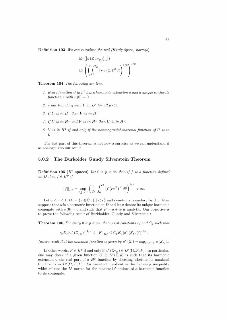
47

Definition 103 We can introduce the real (Hardy Space) norm(s)

E0

(∣∣u (Z.∧TD )∗TD

∣∣)E0

(∫ TD

0

|∇u (Zt)|2 dt

)1/21/2

Theorem 104 The following are true.

1. Every function U in L1 has a harmonic extension u and a unique conjugatefunction v with v (0) = 0

2. v has boundary data V in Lp for all p < 1

3. If U is in H1 then V is in H1

4. If U is in H1 and V is in H1 then U is in H1.

5. U is in H1 if and only if the nontangential maximal function of U is inL1

The last part of this theorem is not now a surprise as we can understand itas analogous to our result.

5.0.2 The Burkolder Gundy Silverstein Theorem

Definition 105 (Hp spaces) Let 0 < p < ∞ then if f is a function definedon D then f ∈ Hp if

||f ||Hp = sup0≤r<1

(1

2π

∫ 2π

0

∣∣f (reiθ)∣∣p dθ)1/p

<∞.

Let 0 < r < 1, Dr = z ∈ C : |z| < r and denote its boundary by Tr. Nowsuppose that u is a harmonic function on D and let v denote its unique harmonicconjugate with v (0) = 0 and such that F = u+ iv is analytic. Our objective isto prove the following result of Burkholder, Gundy and Silverstein :

Theorem 106 For every 0 < p <∞ there exist constants cp and Cp such that

cpE0 [u∗ (ZTD )p]1/p ≤ ||F ||Hp ≤ CpE0 [u∗ (ZTD )

p]1/p

.

(where recall that the maximal function is given by u∗ (Zt) = sup0≤s≤t |u (Zs)|).

In other words, F ∈ Hp if and only if u∗ (ZTD ) ∈ Lp (Ω,F , P ) . In particular,one may check if a given function U ∈ Lp (T, µ) is such that its harmonicextension u the real part of a Hp function by checking whether its maximalfunction is in Lp (Ω,F , P ) . An essential ingedient is the following inequalitywhich relates the Lp norms for the maximal functions of a harmonic functionto its conjugate.


Theorem 107 (Conjugate function inequality) For each 0 < p <∞ thereexists a constant cp such that for any harmonic function u on D with conjugatev such that v (0) = 0 there is a constant cp such that

E0 [v∗ (ZTD )p]1/p ≤ cpE0 [u∗ (ZTD )

p]1/p

.

Let 0 < r < 1, Dr = z ∈ C : |z| < r and denote its boundary by Tr andlet TDr represent the exit time of Brownian motion from Dr. Introduce themaximal functions

F ∗r = F ∗(ZTDr

)= sup

0≤t<∞

∣∣F (Zt∧TDr )∣∣u∗r = u∗

(ZTDr

)= sup

0≤t<∞

∣∣u (Zt∧TDr )∣∣ ,then to prove the conjugate function inequality it suffices to prove for each

0 < r < 1 that E0

[v∗(ZTDr

)p]1/p ≤ cpE0

[u∗(ZTDr

)p]1/pfor some constant cp

which does not depend on r. We do this using the following sequence of results.

Lemma 108 Let (Ft)t≥0 be the filtration generated by Zt∧TD and suppose Sand T are Ft− stopping times such that S ≤ T a.s.. Then

E0

[∣∣u (ZT∧TDr )− u (ZS∧TDr )∣∣2] = E0

[∣∣v (ZT∧TDr )− v (ZS∧TDr )∣∣2] .Proof. Without loss of generality we can (and will) assume F (0) = 0 through-out this and subsequent proofs. Since F 2 is analytic we know F 2 (Zt) is a localmartingale. Moreover, since F is bounded on D it follows that F 2

(Zt∧TDr

)is a bounded martingale and then F 2

(Zt∧S∧TDr

), F 2

(Zt∧T∧TDr

)are bounded

martingales as well. Optional stopping followed by martingale convergence gives(using TDr <∞):

E0

[F 2(Zt∧S∧TDr

)]= E0

[F 2(Z0∧S∧TDr

)]= 0,

limt→∞

E0

[F 2(Zt∧S∧TDr

)]= E0

[F 2(ZS∧TDr

)]= 0.

Consequently,

0 = E0

[u(ZS∧TDr

)2 − v (ZS∧TDr )2]+ 2iE0

[u(ZS∧TDr

)v(ZS∧TDr

)]so E0

[u(ZS∧TDr

)2]= E0

[v(ZS∧TDr

)2]and a similar calculation gives

E0

[u(ZT∧TDr

)2]= E0

[v(ZT∧TDr

)2]. Now s → u

(Zt∧S∧TDr

)is a one di-

mensional real martingale which is bounded (and so UI) so we have

E0

[u(Zt∧T∧TDr

)|FS]

= u(Zt∧S∧TDr

),

and then

E0

[u(Zt∧T∧TDr

)u(Zt∧S∧TDr

)]= E0

[E0

[u(Zt∧T∧TDr

)|FS]u(Zt∧S∧TDr

)]= E0

[u(Zt∧S∧TDr

)2].

49

The same argument also gives this result for the conjugate function v therefore

E0

[∣∣u (ZT∧TDr )− u (ZS∧TDr )∣∣2]= E0

[u(ZT∧TDr

)2 − 2u(ZT∧TDr

)u(ZS∧TDr

)+ u

(ZS∧TDr

)2]= E0

[u(ZT∧TDr

)2 − u (ZS∧TDr )2]= E0

[v(ZT∧TDr

)2 − v (ZS∧TDr )2]= E0

[∣∣v (ZT∧TDr )− v (ZS∧TDr )∣∣2] .

Lemma 109 Suppose g is a measurable function on a measure space (X,B, µ)and E ⊂ X is a measurable set with 0 < µ (E) < ∞ and g ≥ 0 on E. Supposefurther that A and B are constants such that :

1. 1µ(E)

∫Egdµ ≥ A > 0 and

2. 1µ(E)

∫Eg2dµ ≤ B.

Then for any δ ∈ (0, 1) ,

µ x : g (x) ≥ δA ≥ µ (E) (1− δ)2 A2

B.

Proof. Let Eδ = x ∈ E : g (x) ≥ δA , then∫E\Eδ

gdµ ≤ δAµ (E)

so 1 gives

Aµ (E) ≤∫E

gdµ =

∫E\Eδ

gdµ+

∫Eδ

gdµ ≤ δAµ (E) +

∫Eδ

gdµ

and hence ∫Eδ

gdµ ≥ (1− δ)Aµ (E) .

But Cauchy-Schwarz and 2 give that∫Eδ

gdµ ≤(∫

Eδ

g2dµ

)1/2

µ (Eδ)1/2

,

so that

µ (Eδ) ≥A2

B

(1− δ2

)µ (E) .


Lemma 110 Let a ≥ 1 and b > 1. There are constants ca,b and da,b such thatif λ > 0 and

P (F ∗r > λ) ≤ aP (F ∗r > bλ) ,

thenP (F ∗r > λ) ≤ ca,bP (u∗r > bλ) .

Proof. Define the stopping times S = inft ≥ 0 :

∣∣F (Zt∧TDr )∣∣ > λ

and T =

inft ≥ 0 :

∣∣F (Zt∧TDr )∣∣ > bλ, so that S ≤ T a.s.. On the set F ∗r > bλ =

T <∞ we have that∣∣F (ZS∧TDr )∣∣ = λ and

∣∣F (ZT∧TDr )∣∣ = bλ.Also, F ∗r ≤ λ =S = T =∞ and so on this set we must have ZS∧TDr = ZT∧TDr = ZTDr . Fromlemma 109 we deduce that

E0

[∣∣u (ZT∧TDr )− u (ZS∧TDr )∣∣2 1F∗r >λ

]= E0

[∣∣u (ZT∧TDr )− u (ZS∧TDr )∣∣2]=

1

2E0

[∣∣F (ZT∧TDr )− F (ZS∧TDr )∣∣2]≥ 1

2E0

[∣∣F (ZT∧TDr )− F (ZS∧TDr )∣∣2 1F∗r >bλ

]=

1

2λ2 (b− 1)

2P (F ∗r > bλ) ≥ λ2 (b− 1)

2

2aP (F ∗r > λ) .

Also,

E0

[∣∣u (ZT∧TDr )− u (ZS∧TDr )∣∣4 1F∗r >λ

]≤ E0

[∣∣F (ZT∧TDr )− F (ZS∧TDr )∣∣4 1F∗r >λ

]= E0

[∣∣F (ZT∧TDr )− F (ZS∧TDr )∣∣4 1F∗r >bλ

]+E0

[∣∣F (ZT∧TDr )− F (ZS∧TDr )∣∣4 1λ<F∗r ≤bλ

]≤ λ4 (b+ 1)

4P (F ∗r > bλ) + 16b4λ4P (λ < F ∗r ≤ bλ)

≤(

(b+ 1)4

+ 16b4)λ4P (F ∗r > λ) .

Applying lemma 109 for the choice

g =∣∣u (ZT∧TDr )− u (ZS∧TDr )∣∣2 , E = F ∗r > λ ,

A =λ2 (b− 1)

2

2aand B =

((b+ 1)

4+ 16b4

)λ4,

we see that for any δ ∈ (0, 1)

P (F ∗r > λ) ≤ B

A2(1− δ2

)P∣∣u (ZT∧TDr )− u (ZS∧TDr )∣∣ ≥

(δ (b− 1)

2

2a

)1/2

λ

.

Fixing a value of δ and observing that∣∣u (ZT∧TDr )− u (ZS∧TDr )∣∣ ≤ 2u∗r finishes

the result.

51

We can now present :Proof. (of lemma 107) Fix p ∈ (0,∞) . For x ≥ 0 let G (x) = P (F ∗r > x) then

E [|F ∗r |p] = −

∫ ∞0

λpG (dλ) .

Since F is bounded we have G (x) = 0 for all x large enough and so integrationby parts gives

E [|F ∗r |p] =

∫ ∞0

G (λ) pλp−1dλ =

∫ ∞0

pλp−1P (F ∗r > λ) dλ.

Let a = 2p+1 and b = 2. If B denotes the set of all λ > 0 for which

P (F ∗r > λ) ≤ aP (F ∗r > bλ)

then ∫ ∞0

pλp−1P (F ∗r > λ) dλ =

∫ ∞0

p(bx)p−1P (F ∗r > bx) bdx

= bp

(∫B

pxp−1P (F ∗r > bx) dx+

∫[0,∞)\B

pxp−1P (F ∗r > bx) dx

)

≤ bp

(∫B

pxp−1P (F ∗r > bx) dx+1

a

∫[0,∞)\B

pxp−1P (F ∗r > x) dx

)

= bp∫B

pxp−1P (F ∗r > bx) dx+bp

a

∫ ∞0


−bp

a

∫B

pxp−1P (F ∗r > x) dx,

so that(1− bp

a

)∫ ∞0

pxp−1P (F ∗r > x) dx ≤ bp(

1− 1

a

)∫B


and ∫ ∞0

pxp−1P (F ∗r > x) dx ≤bp(1− 1

a

)(1− bp

a

) ∫B


≤ a

∫B

pxp−1P (F ∗r > x) dx.

Thus an application of lemma 110 gives

E [|F ∗r |p] ≤ a

∫B


≤ a

∫B

pxp−1ca,bP (u∗r > da,bx) dx

≤ aca,bda,b

∫ ∞0

pxp−1P (u∗r > x) dx

= cpE [|u∗r |p] ≤ cpE [|u∗|p] .


Remark 111 In the course of the proof we have actually shown the strongerresult that E [|v∗r |

p]≤ cpE [|u∗r |

p] for all r ∈ (0, 1) .

As a corollary of this result we can obtain Riesz’s inequalities relating theHp-norms of the harmonic function with its conjugate.

Corollary 112 (Riesz’s Inequality) For each p ∈ (1,∞) there is a constantcp, which does not depend on r, such that whenever u is harmonic on D and vis its harmonic conjugate with v (0) = 0 and r ∈ (0, 1) ,

1

2π

∫ 2π

0

∣∣v (reiθ)∣∣p dθ ≤ cp2π

∫ 2π

0

∣∣u (reiθ)∣∣p dθ.Proof. Again let F = u + iv. By conformal invariance F

(Zt∧TDr

)is a time

changed Brownian motion and since F is bounded it is a martingale. It followsat once that u(Zt∧TDr ) is martingale and hence (conditional Holder + Jensen

with x 7−→ |x|p)∣∣u (Zt∧TDr )∣∣p is a submartingale if p ∈ (1,∞) . Doob’s maximal

inequality then gives

E

[sup

0≤t<∞

∣∣u (Zt∧TDr )∣∣p] ≤ ( p

p− 1

)pE[∣∣u (ZTDr )∣∣p] .

Now using the conjugate function inequality and the above gives

1

2π

∫ 2π

0

∣∣v (reiθ)∣∣p dθ = rE[∣∣v (ZTDr )∣∣p]

≤ rE [(v∗r )p]

≤ rcpE [(u∗r)p]

≤ rcp

(p

p− 1

)pE[∣∣u (ZTDr )∣∣p]

= cp

(p

p− 1

)p1

2π

∫ 2π

0

∣∣u (reiθ)∣∣p dθ.

We may now prove the Burkholder Gundy Silverstein result :Proof. (of theorem 106) We first notice that

1

2π

∫ 2π

0

∣∣v (reiθ)∣∣p dθ = rE[∣∣v (ZTDr )∣∣p] ≤ rE [(v∗r )

p]

and similarly for v. The right hand inequality then follows almost immediatelyfrom the conjugate function inequality :

1

2π

∫ 2π

0

∣∣F (reiθ)∣∣p dθ ≤ 1

2π

∫ 2π

0

2p(max

∣∣u (reiθ)∣∣ , ∣∣v (reiθ)∣∣)p dθ≤ 2p

2π

∫ 2π

0

(∣∣u (reiθ)∣∣+

∣∣v (reiθ)∣∣)pdθ≤ cpE [(u∗r)

p] .

53

We now prove the left hand inequality. To do this suppose F ∈ Hp then itfollows from the lemma below that

(|F(Zt∧TDr

)|p/2)t≥0

is a submartingale.

Doob’s maximal inequality then gives

E [(u∗r)p] ≤ E

[(sup

0≤t<∞|F(Zt∧TDr

)|p/2)2]

≤ cpE[∣∣F (ZTDr )∣∣p]

=cp

2πr

∫ 2π

0

∣∣F (reiθ)∣∣p dθ,where the second line is established by the same reasoning as in Riesz’s inequalities.Letting r → 1 and using monotone convergence gives

E [(u∗)p] ≤ cp lim

r→1

1

2πr

∫ 2π

0

∣∣F (reiθ)∣∣p dθ≤ cp sup

0≤r<1

(∫ 2π

0

∣∣F (reiθ)∣∣p dθ) .To finish we need to show that

(|F(Zt∧TDr

)|p/2)t≥0

is a submartingale. This

is accompolished using a result of Doob, for which one needs the notion of asubharmonic function :

Definition 113 A continuous function φ defined on a domain U ⊂ C is said tobe subharmonic if for every z ∈ U there is an R such that if ζ : |ζ − z| ≤ R ⊂U and

φ (z) ≤ 1

2π

∫ 2π

0

φ(z + reiθ

)dθ for all r ∈ (0, R) .

Remark 114 If F ia analytic on U and c > 0 then |F |c is subharmonic on U .

The fact that(|F(Zt∧TDr

)|p/2)t≥0

is a submartingale is then seen by com-

bining this remark with:

Lemma 115 If φ is subharmonic on Dr and continuous on Dr, then(φ(Zt∧TDr

))t≥0

is a submartingale.

Proof. See Petersen chapter 6.

Bibliography

[1] Ahlfors, Lars V., Complex analysis: An introduction of the theory of ana-lytic functions of one complex variable. Second edition McGraw-Hill BookCo

[2] Bass, Richard F., Probabilistic techniques in analysis. Springer-Verlag, NewYork, 1995

[3] Burkholder, D. L.; Gundy, R. F.; Silverstein, M. L,. A maximal functioncharacterization of the class Hp. Trans. Amer. Math. Soc. 157 1971 137–153.

[4] Carne, T. K., Brownian motion and Nevanlinna theory. Proc. LondonMath. Soc. (3) 52 (1986), no. 2, 349–368

[5] Davis, Burgess, Brownian motion and analytic functions. Ann. Probab. 7(1979), no. 6, 913–932.

[6] Gruet, J.-C. ; Mountford, T. S. , The rate of escape for pairs of windingson the Riemann sphere, J. London Math. Soc. (2) 48 (1993), no. 3, 552–564

[7] Herz, Carl, Hp-spaces of martingales, 0 < p < 1, . Z. Wahrscheinlichkeits-theorie und Verw. Gebiete 28 (1973/74), 189–205.

[8] Lyons, T. J.; McKean, H. P. Winding of the plane Brownian motion. Adv.in Math. 51 (1984), no. 3, 212–225.

[9] McKean, Henry P. Stochastic integrals. Reprint of the 1969 edition, witherrata. AMS Chelsea Publishing, Providence, RI, 2005.

[10] McKean, H. P.; Sullivan, D. Brownian motion and harmonic functions onthe class surface of the thrice punctured sphere. Adv. in Math. 51 (1984),no. 3, 203–211

[11] Mountford, T. S. Transience of a pair of local martingales. Proc. Amer.Math. Soc. 103 (1988), no. 3, 933–938.

[12] Petersen, Karl Endel, Brownian motion, Hardy spaces and bounded meanoscillation. London Mathematical Society Lecture Note Series, No. 28.Cambridge University Press, Cambridge 1977

55

56 BIBLIOGRAPHY

Index

Cauchy Riemann Equation , 3

Doob, vii, viii

entire function, 4

Fundamental Theorem of Algebra, 5

Integral Representation Formula, 4

Kolmogorov, vii

Laplace equation, viiLouiville’s Theorem, 4

martingale, vii

Picard’s Theoremstatement, 6

Schramm, viiSLE, see Stochastic Loewner EquationStochastic Loewner Equation, vii

57

C10.1b { { 16HT Brownian Motion in Complex...

Documents

Transcript of C10.1b { { 16HT Brownian Motion in Complex...