c© 2017 Siddhartha Nigam

QUANTIFICATION OF BENEFITS OF THE CAMPUS GRIDOPERATIONS AS A MICROGRID

BY

SIDDHARTHA NIGAM

THESIS

Submitted in partial fulfillment of the requirementsfor the degree of Master of Science in Electrical and Computer Engineering

in the Graduate College of theUniversity of Illinois at Urbana-Champaign, 2017

Urbana, Illinois

Adviser:

Professor George Gross

ABSTRACT

The US grid’s weak ability to withstand severe weather incidents, particu-

larly with the growing number of events due to climate change, the slow pace

of expansion of transmission grids and the increased push to integrate deeper

penetrations of renewable resources in recent years, has raised many questions

about the reliability and resilience of the electricity supply as well as about

the design and operational paradigm of the distribution grid. The increased

implementation of microgrids (µgs) in distribution networks (DN s) indicates

that µgs provide promising alternative approaches to address many of these

issues. The growing interest in µg implementations provides evidence that

many projects are, in effect, able to realize such benefits. However, the lack

of a general methodology that can comprehensively quantify the benefits of

applying the µg concept to any power system limits the much broader im-

plementation of µgs as the investments made in the µg area are not justified.

In light of this situation, we developed a quantification methodology and

carried out the quantification and comparative analysis of the benefits of the

operation of the University of Illinois at Champaign-Urbana (UIUC ) cam-

pus utility system (CUS ) as a µg versus its current operations. The UIUC

campus is a microcosm of a city with diverse facilities including the academic

buildings and laboratories, student housing facilities, theatres, health center,

sports stadiums, libraries, veterinary hospital and an airport. The UIUC

campus is critically dependent on the CUS for its chilled water, steam and

electricity demands year round. The UIUC CUS has all the required char-

acteristics of a µg including distributed energy resources (DERs), critical

and non–critical loads and a defined electrical grid boundary. Thus, we may

view the CUS as a µg. Consequently, consideration of the UIUC CUS via

µg optics allows us to carry out a comparative quantification of the benefits

of the UIUC CUS operated as a µg versus under the current operational

paradigm.

ii

For the quantification methodology, we use a stochastic simulation ap-

proach that provides the capability to quantify the impacts of CUS oper-

ations in terms of economic, reliability and emissions metrics of the CUS

operations under a specified operational paradigm. The approach is based

on the explicit representation of the various sources of uncertainty together

with the time-varying nature in the demand–side and supply–side resources

in the CUS. The simulation approach models the uncertainty in the demands,

available capacity of conventional generation resources and the time–varying,

intermittent renewable resources in terms of discrete–time random processes

(r.p.s). Such a representation explicitly takes into account the time correla-

tions in each input variable. A key exponent of the simulation approach is the

formulation of the so–called energy scheduling optimization problem (ESOP).

The ESOP solution is an essential building block in our approach and is used

to determine the CUS resource scheduling decisions with the explicit consid-

eration of the uncertainty effects. Under the current operational paradigm,

the schedule of the energy resources is based on heuristic techniques and

does not involve the deployment of formal optimization techniques. The

ESOP solution replaces the current heuristics–based approach to determine

the optimal schedule and loading levels of the CUS energy resources so as

to minimize the CUS operational costs. We use this optimal scheduling as a

proxy for the current operational paradigm. In this way we can carry out on

a consistent basis a comparative analysis of the UIUC CUS operational per-

formance as a µg – the so–called µg operational paradigm – and those under

the optimal operations of the current paradigm. A modified ESOP and its

solution is also adopted in the simulation methodology for the quantification

of the CUS operational performance under the µg operational paradigm. A

salient feature of the ESOP mathematical formulation is its ability to capture

the inter–dependencies in the electricity and steam services that the UIUC

CUS provides under each operational paradigm. The simulation approach

makes use of the Monte Carlo simulation (MCS ) techniques to represent the

impacts of sources of uncertainty on the CUS operations under each opera-

tional paradigm. As such, we systematically sample the r.p.s to generate the

realizations, or sample paths, that we use to emulate the scheduling of the

CUS for a given operational paradigm via the ESOP. The ESOP solution

maps the sample paths of the loads and supply resources into the sample

paths of the r.p.s we use to measure the performance of CUS operations.

iii

The evaluation of the metrics of interest is based on these resulting s.p.s.

We demonstrate the capabilities of the simulation approach by carrying

out various case studies on the UIUC CUS. We discuss a set of representa-

tive studies to gain important insights about the current UIUC CUS oper-

ations and under the application of the µg concept to the UIUC CUS. The

studies provide clear understanding of the interactions between the electric

and steam utility in the UIUC CUS and the limitations on electric system

operations imposed by the requirement to meet the steam loads. A key ob-

servation made from these case studies is that the extent of the benefits of

the µg concept application to a power system attained would depend on

the characteristics of the system as well as the location of the system in the

geographical footprint of the distribution system.

There is a broad range of applications of this methodology, including re-

source planning studies, reliability, economic and environmental assessments

and operational studies. A particularly attractive feature is its ability to pro-

vide answers to various “what if ” questions of any nature. The methodology

described in this thesis is general in a sense that it can easily be adapted to

demonstrate the extent to which the benefits of the µg concept application

can be realized in any particular power system when it is operated as a µg

versus when it is operated under its current paradigm.

iv

To Ma, Papa, Archita and Prutha, for their love and support.

v

ACKNOWLEDGMENTS

I would like to thank my advisor, Prof. George Gross, for the guidance, dedi-

cation and support he provided throughout my master’s work. His attention

to detail and high standards have helped me develop a critical eye towards

research and become a better student. I am also thankful to all the professors

and staff in the Power and Energy Systems group at ECE UIUC who have

helped me time and again during my master’s work.

I would like to express my gratitude to Adriano, Archana, Dipanjan,

Hanchen, Mariola, Raj and all the other students in the Power and Energy

Systems group for the great time and wonderful moments spent together

laughing and learning which has made my master’s experience memorable.

Finally, I would like to thank Prutha, Archita, Ma and Papa for constantly

believing in me and helping me face difficulties and challenges head–on with

a smile on my face. I feel extremely fortunate to have you all in my life.

vi

TABLE OF CONTENTS

LIST OF FIGURES . . . . . . . . . . . . . . . . . . . . . . . . . . . . ix

CHAPTER 1 INTRODUCTION . . . . . . . . . . . . . . . . . . . . 11.1 State of the Art . . . . . . . . . . . . . . . . . . . . . . . . . . 31.2 Motivation to the Quantification Problem and Scope of the

Work . . . . . . . . . . . . . . . . . . . . . . . . . . . . . . . . 51.3 Summary . . . . . . . . . . . . . . . . . . . . . . . . . . . . . 9

CHAPTER 2 UIUC CAMPUS UTILITY SYSTEM THROUGHMICROGRID OPTICS . . . . . . . . . . . . . . . . . . . . . . . . . 112.1 The UIUC CUS . . . . . . . . . . . . . . . . . . . . . . . . . 112.2 CUS Operations under the Current Paradigm . . . . . . . . . 182.3 UIUC CUS Operations under the µg Framework . . . . . . . 192.4 Summary . . . . . . . . . . . . . . . . . . . . . . . . . . . . . 21

CHAPTER 3 METHODOLOGY FOR THE QUANTIFICATIONOF THE CUS OPERATIONAL PERFORMANCE . . . . . . . . . 233.1 Quantification Methodology Overview . . . . . . . . . . . . . . 243.2 ESOP . . . . . . . . . . . . . . . . . . . . . . . . . . . . . . . 283.3 Simulation Methodology Description . . . . . . . . . . . . . . 343.4 Evaluation of Performance Metrics . . . . . . . . . . . . . . . 363.5 Summary . . . . . . . . . . . . . . . . . . . . . . . . . . . . . 37

CHAPTER 4 QUANTIFICATION STUDIES . . . . . . . . . . . . . 394.1 Overview of the Study . . . . . . . . . . . . . . . . . . . . . . 414.2 Comparison of the CUS Operational Performance for the

Base and PSSF Case . . . . . . . . . . . . . . . . . . . . . . . 434.3 Summary . . . . . . . . . . . . . . . . . . . . . . . . . . . . . 52

CHAPTER 5 CONCLUDING REMARKS . . . . . . . . . . . . . . . 545.1 Summary . . . . . . . . . . . . . . . . . . . . . . . . . . . . . 545.2 Possible Directions For Future Research . . . . . . . . . . . . 56

APPENDIX A REVIEW OF THE MICROGRID CONCEPT ANDANALYTICAL FRAMEWORK . . . . . . . . . . . . . . . . . . . . 58

vii

APPENDIX B LIST OF SYMBOLS . . . . . . . . . . . . . . . . . . 62B.1 General Variables . . . . . . . . . . . . . . . . . . . . . . . . . 62B.2 Steam–Based Variables and Parameters . . . . . . . . . . . . . 62B.3 Electricity–Based Variables and Parameters . . . . . . . . . . 63B.4 Electricity Grid Variables and Parameters Notations . . . . . . 63B.5 Simulation Variables and Parameter Notations . . . . . . . . . 64

REFERENCES . . . . . . . . . . . . . . . . . . . . . . . . . . . . . . . 66

viii

LIST OF FIGURES

1.1 Key drivers to the µg concept . . . . . . . . . . . . . . . . . . 2

2.1 The campus electricity daily load shapes for a week in March2015 (a) and September 2015 (b) . . . . . . . . . . . . . . . . 13

2.2 The campus steam daily load shapes for a week in January2015 (a) and August 2015 (b) . . . . . . . . . . . . . . . . . . 14

2.3 The schematic of the Abbott power plant layout . . . . . . . . 162.4 Phoenix Solar South Farm . . . . . . . . . . . . . . . . . . . . 162.5 Simple single line diagram of the campus electricity grid . . . 172.6 UIUC campus as a µg . . . . . . . . . . . . . . . . . . . . . . 21

3.1 The time frame used in simulation approach with the sub-periods of a simulation period Ti indicated . . . . . . . . . . . 26

3.2 Conceptual structure of the simulation approach . . . . . . . . 273.3 Monte Carlo simulation: conceptual flow chart . . . . . . . . . 35

4.1 Side–by–side comparison of the reliability of electricity sup-ply, emissions and economics metrics for the CUS opera-tions under the two operational paradigms . . . . . . . . . . . 40

4.2 Average daily production costs for the base case . . . . . . . . 454.3 Average daily LOLP for the base case . . . . . . . . . . . . . . 464.4 Average daily CO2 emissions for the base case . . . . . . . . . 474.5 Average daily energy production costs for the PSSF case . . . 494.6 Average daily LOLP for the PSSF case . . . . . . . . . . . . . 504.7 Average daily CO2 emissions for the PSSF case . . . . . . . . 504.8 Average hourly marginal cost to supply steam for an av-

erage day in Jan–Mar for CUS operations under the µgoperational paradigm for base and PSSF case . . . . . . . . . . 51

4.9 Average hourly marginal cost to supply steam for an aver-age day in Jul–Sep months for CUS operations under theµg operational paradigm for base and PSSF case . . . . . . . . 52

A.1 µg analytical framework . . . . . . . . . . . . . . . . . . . . . 61

ix

CHAPTER 1

INTRODUCTION

The US grid is increasingly subject to extreme weather incidents, e.g., the

superstorm Sandy in 2012, which caused serious damage with major social

and financial impacts. From 2003 to 2012, roughly 679 power outages oc-

curred due to weather events with each affecting at least 50,000 consumers;

these outages have estimated annual average costs of $ 18–33 billion in 2014

$ [1]. The number of outages due to weather is expected to rise as climate

change leads to higher frequency and intensity of hurricanes, blizzards, floods

and other extreme weather events.

The growth in future electricity demand requires the expansion of the

generation/transmission system. Furthermore, the deepening penetration of

integrated renewable resources into the grid increases the need for the trans-

mission expansion and also for effective operational procedures to manage

the variability and intermittency in the renewable energy outputs [2]. The

small number of new transmission projects implies that the many technology

advancements and the smart grid implementation have yet to be deployed in

many parts of today’s legacy grid. Congestion results whenever the demand

for transmission services exceeds the grid’s capability to provide; such sit-

uations occur frequently in current electricity markets. Despite the more

intense utilization of the grid by the many established and new players,

developments in transmission expansion have failed to keep pace with the

increasing demand.

Given the status of the grid and the difficulties in overcoming the chal-

lenges in transmission expansion, the ability to connect resources at the

distribution level in order to improve electricity supply reliability appears

to provide a promising alternative. Resources connected at sub-transmission

and distribution voltage levels – the so–called distributed energy resources

(DERs) – include distributed generation (DG), demand response (DR) and

energy storage (ES ) resources. Deeper DER penetration necessitates im-

1

proved schemes to manage and utilize effectively the energy, capacity and

ancillary service contributions of DERs to the grid. This need aligns with

the vision of the smart grid concept which is to develop a modernized electric-

ity delivery system that monitors, protects and automatically optimizes the

operation of all its interconnected elements from the central and distributed

generators through the high-voltage transmission grid and the distribution

network (DN ), to industrial users and building automation systems, to en-

ergy storage devices and to end–use consumers and their thermostats, electric

vehicles, appliances and other devices.

Despite the deepening penetration of DERs over the years, we have not

fully utilized their services owing to the IEEE 1547 standard which does

not allow the DGs to island and operate under an outage. Some of the

key issues discussed above are the drivers for the need of a new concept or a

new paradigm of grid operations that meets the requirements from the smart

grid vision i.e., to not only enable the deep penetration of DERs but also

optimally utilize the services provided by the DERs at all times to maximize

customer benefits with the desired electricity supply reliability [3], [4]. This

new concept is the µg concept and its key drivers are illustrated in the Figure

1.1.

Figure 1.1: Key drivers to the µg concept

Deployment of µgs in the distribution network (DN ) is seen as a promising

2

approach to address some issues in the current electricity system. A µg1 is a

network of interconnected loads and DERs, within clearly defined geographic

boundaries, with the properties that it is a single controllable entity with

respect to the grid and that it operates either connected to or disconnected

from the distribution grid, i.e., in either the parallel/grid–connected or in

the islanded/isolated mode [5]. µg loads may be classified as either critical

loads or non–critical loads [6]. The classification is essential for supply–

demand balance under the islanded mode of operation. In Appendix A of

this thesis, we provide a detailed review of the µg concept and develop an

analytical framework that fits the various implementations of the µg such

as the campus µg, community µg. We make use of the µg concept and the

analytical framework for the better understanding of work presented in this

thesis.

1.1 State of the Art

The claimed benefits in various µg projects gave rise to considerable interest

in µgs everywhere. The rapid pace of µg development has resulted in a broad

range of projects that vary from a few kW to several MW, depending on the

specific application and the desired benefit. The effective exploitation of µg

salient characteristics may result in a wide range of benefits from grid relia-

bility improvement to electricity supply cost reduction and from facilitation

of renewable energy integration to reduction in environmental impacts [7],[8]

and [9].

The reliability of an electric supply system is defined as the probability of

assurance to provide the consumers with continuous service with satisfactory

quality (with voltages and frequency within prescribed bounds) [10]. Upon

the onset of severe weather events, a µg may unilaterally island itself from

its DN to supply electricity from the µg DGs to the critical loads within

its boundary. Under situations when the µg DGs fail, the DN acts as the

only backup to supply the µg loads. The two modes of operations ensure

that the electricity supply to the µg critical loads is maintained; absent the

1A special class of µg is the autonomous µg. An autonomous µg is a network of inter-connected loads and DERs, within clearly defined geographic boundaries, whose salientproperty is its operation disconnected from a grid, i.e., in the islanded mode at all times.This thesis does not deal with the autonomous µgs.

3

two modes of operation and classification of µg loads into critical and non–

critical loads, all the loads remain unserved. During hurricane Sandy, 1.9

million people lost power in NY city as Con Ed had to shut down its gen-

eration units to prevent any further damage to its facilities due to flooding.

The NYU µg, consisting of the co-generation plant and the nearby building

loads, was islanded from the Con Ed grid. The underground natural gas

grid lines supplied the fuel to NYU µgs natural–gas–powered generators to

produce electricity. During the hurricane, electricity supply was maintained

continuously to the loads in buildings in close proximity of the NYU µgs

co-generation plant, which did not flood. Built for the purpose to reduce en-

ergy costs, NYU s cogeneration plant was able to operate as a µg to maintain

the continuity of supply during and after hurricane Sandy. The Princeton

University µg has 4 connections with the PSE&G grid. The supply through

two connections was lost due to damage to the upstream2 network during

hurricane Sandy. The µg isolated itself from the PSE&G grid by opening

the switches at all 4 connection points and used its generation to supply its

loads.

A µg that operates in the parallel mode may sell any surplus generation

to the DN and receive payment as stipulated by the legislative/regulatory

policy of the jurisdiction in which it is located. Since a µg can exercise con-

trol over all its DERs and loads, it may serve as a DR resource or provide

frequency control ancillary services as long as the µg has adequate gener-

ation and load resources to participate in the bulk electricity markets in

accordance with FERC Order No. 764. The additional revenues from such

services may allow further reduction of the supply costs of electricity to the

µg loads. For example, Princeton University µg participates in the PJM

wholesale ancillary services markets to offer frequency control services [11].

In addition, the Princeton University µg buys much of its energy required

by its loads in the PJM wholesale markets whenever the PJM prices are

below the Princeton µgs generation costs. However, when Princeton µg can

produce less expensive energy than PJM, the µg generators operate to meet

as much of the electricity needs of the university as possible and if there is

surplus generation, the µg sells energy to earn revenues.

The impacts of climate change are key drivers of the increased deploy-

2Check Appendix A on the µg framework for the definitions of the upstream and thedownstream network

4

ment of renewable resources to reduce CO2 emissions. In various venues,

legislative/regulatory initiatives stipulate specific renewable portfolio stan-

dards (RPS ) targets and dates that must be met to bring about a cleaner

environment. At deeper wind and solar resource penetrations, operators

must rely to a greater extent on the controllable resources to manage wind

and solar output variability and intermittency. Also, controllable resources

must have adequate ramping capability to appropriately manage the rapid

changes in the renewable resource outputs so that supply-demand balance is

kept around the clock. The integration of large volumes of renewable resource

outputs at high voltage levels, such as large wind or solar farms, increases the

need for transmission expansion so as to allow the wheeling of the electricity

from the farms to areas that desire the clean generation outputs. µgs have a

considerably smaller geographical footprint and demand than the entire grid

and hence are more manageable. Therefore, the management of rapid varia-

tions including the intermittency in the renewable resource outputs is easier

in a µg through the effective coordination of storage and demand resources

with the renewable outputs. Thus, the µgs provide a manageable solution at

lower voltage levels to integrate renewable resources. The carbon footprint

of a particular power system depends on the resource mix and system opera-

tions. If a particular power system has a large fraction of renewable projects

in its resource mix, the renewable generation may displace a larger fraction

of the fossil–fuel–fired generation to result in a smaller carbon footprint. As

the integration of renewable resources is manageable in a µg, the resource

mix of many µg implementations such as the Santa Rita Jail µg includes

renewable resources [12]. The integrated renewable resources displace some

portion of the fossil–fuel–fired generation and consequently reduce the µg

carbon footprint.

1.2 Motivation to the Quantification Problem and

Scope of the Work

The current literature claims that µgs provide a new paradigm to operate a

power system. The recent µg implementations suggest that the deployment

and effective utilization of µgs in the power system may lead to benefits such

as the improvement of reliability of electricity supply, reduction in electricity

5

supply costs and reduction in the carbon footprint. To bring about large-

scale deployment of µgs in order to effectively harness such claimed benefits,

a major challenge is to identify appropriate incentives for the construction

of µgs in the grid. There is need for a proper quantification of µg benefits

that may aid the identification and formulation of the appropriate incentives

directly aligned with the benefits. As such, the assessment of the µg benefits

on an analytical level is well addressed in the current literature but such an

analytical assessment cannot justify any future investments in µgs. Thus,

there is a need for a methodology to quantify the above–mentioned highly

touted µg benefits. In light of the considerable interest that is taken in the µg

area due to the potential benefits and the need to justify any future financial

investments in this area or promote any incentives to construct and deploy

µgs, there is an acute need for a methodology that can reproduce with good

fidelity the expected variable effects – in terms of economics, reliability and

emissions – of any power system operated as a µg when compared to the

same power system operated as is.

There are not many papers in the current literature that provide a com-

prehensive study on the quantification of µg benefits. [13],[14] and [15] assess

and quantify the improvements in the reliability of electricity supply of the

µg loads but do not discuss the impacts of µg concept application on the

economics and emissions aspects. The authors in [16] provide interesting

insights about µg resource scheduling strategies that can be used in µg op-

erations such as operating the µg to achieve minimum cost of operation or

minimum emissions production. The authors in [16] evaluate the benefits but

do not take into account the uncertainty in the µg operations while doing

the quantification and do not apply the quantification methodology over a

considerable period of time, thereby failing to capture the seasonal effects on

the power system operations. Moreover, the authors compare the computed

emissions and economic metrics among the various µg resource scheduling

strategies used in the paper rather than comparing the metrics with those of

a case where the system is not operated as a µg. In [17],[18], the comparison

of the quantified benefits of a power system operation with and without the

µg concept application is done without keeping the resource mix constant

and hence the benefits are accounted to the resource mix change rather than

the µg. More specifically, in these two papers the metrics for emissions and

economics are computed and compared for varying level of DG penetration

6

in the resource mix of the µg. In [19], the authors claim to make use of three

cases for computation of reliability, economic and emission metrics: first

where a feeder in a DN has no DGs, second with DGs and third when the

feeder with DGs operated in a µg. The authors compare the case 1 results

with case 2 and case 3 together and the results for case 2 and case 3 are not

given separately. As such, the authors show the improvements in emissions,

economics and reliability due to the deployment of DGs in DN but not due

to the µg concept application.

In this thesis, we aim to learn the extent to which the µg benefits would

accrue to a power system if it were to be operated as a µg without any

change in the resource mix. We seek to quantify the impacts of the µg con-

cept application on the economics, reliability and emission variable effects of

power system operations and compare the metrics for economics, reliability

and emissions when the same power system is operated as is. For a consis-

tent comparison, we need a systematic and a comprehensive quantification

methodology that uses appropriate metrics to quantify the benefits of the µg

concept application to a power system, takes into account the uncertainties

involved in power system operations and is applicable over different periods

of time to capture the seasonal impacts and comprehensively understand the

value that a µg brings to the system. Thus, we report the development

of a practical and a comprehensive simulation–based methodology that can

reproduce with good fidelity the expected variable effects in terms of eco-

nomics, reliability and emissions of a power system when operated as is

and as as a µg. We deploy this methodology on the UIUC CUS for the

quantification and comparison of the benefits of the operation of the CUS

as a µg (the µg operational paradigm) versus when the UIUC CUS is op-

erated as is (the current operational paradigm). The µg operations involve

coordinated control over the supply–side and demand–side resources with

optimal scheduling of the resources unlike the current operational paradigm.

Therefore, for a consistent quantitative comparison of the CUS operational

performance, we make use of the optimal operations of the current opera-

tional paradigm as a proxy for the current paradigm. The UIUC campus is

a microcosm of a city with diverse facilities including the academic buildings

and laboratories, student housing facilities, theaters, health center, sports

stadiums, libraries and an airport. The UIUC campus is critically depen-

dent on the CUS for the effective operation of this microcosm. We view the

7

utility services provided on campus as an integrated utility system. The CUS

serves the campus demands for the steam, electricity and chilled water year

round. The three services are highly interdependent. If transformed into a

µg framework, the campus would represent a unique case of a µg implemen-

tation. The UIUC CUS meets all the required characteristics of a µg as it

has distributed energy resources (DERs), critical and non–critical loads and

can be conceptually transformed into a µg framework. Such a transforma-

tion allows us to carry out a comparative quantification of the benefits of the

UIUC CUS operated as a µg versus when the UIUC CUS is not operated

as a µg.

The input variables in the simulation, namely the system demand and the

supply resources, are modeled as discrete time random processes (r.p.s) – a

representation that explicitly takes into account the time correlations in each

input variable. The sample paths (s.p.s) of the input r.p.s are constructed

from available historical demand and generation data of hourly time resolu-

tion and for a specified period of time that can be appropriately adjusted

based on the particular requirements of each study. The evaluation frame-

work makes use of the Monte Carlo simulation (MCS ) techniques for the

efficient sampling of the input r.p.s [20]. We make use of the solution to the

so called ESOP2, to map the input r.p.s to the realizations of the output

r.p.s under a given operational paradigm. The realizations of the output

r.p.s are the realizations of operational performance metrics for the UIUC

CUS operated under a given operational paradigm. We statistically approx-

imate the generated realizations of the metrics and assess the performance of

the UIUC CUS operated under a given operational paradigm. We carry out

the side–by–side comparison of the operational performance of UIUC CUS

operated under the optimal operations of the current paradigm and the µg

operational paradigm and demonstrate quantitatively the extent to which µg

benefits are realized as we operate UIUC CUS as a µg. The resource mix is

kept constant3 in the quantitative comparison that we do on the UIUC CUS.

The developed simulation methodology is general in the sense that it can

be easily adapted to quantify the operational performance of any other power

2We discuss the formulation of the ESOP in Chapter 3 in detail.3A major point to understand with regard to µgs is that they only bring a change in

the way a power system is operated. Therefore, the comparison of benefits of operatingthe UIUC CUS as a µg with those when the UIUC CUS is operated as is must be donewith the resource mix kept constant to have a valid comparison.

8

system operated. The simulation methodology is comprehensive as it enables

the appropriate representation of the uncertainty and time-varying nature in

the demand–side and supply–side resources in the system; in particular, the

methodology captures the variability and intermittency in the renewable gen-

eration outputs. The simulation methodology is applicable over any period of

time, thereby capturing the impacts of seasonal variations and maintenance

schedules. In addition, our methodology also allows us to understand the im-

pacts on the system operational performance by answering the various “what

if ” questions including what if there is a change in the resource mix, mainte-

nance schedules in the operation of the system, change in the policy etc. Our

methodology can be easily adapted to incorporate various stochastic models

to represent the time–varying demands, renewable resource outputs and con-

ventional generator available capacities. Our approach, while relatively easy

to implement, can handle any type of renewable output probability distribu-

tion as our methodology does not require any assumptions on the shape of

the distributions. The methodology is applicable to the quantification of the

operational performance of any configuration of the µg/ with any resource

mix.

1.3 Summary

This thesis contains four additional chapters and two appendices. In chapter

2, we describe the UIUC campus, which is a microcosm of a city with diverse

facilities including the academic buildings and laboratories, student housing

facilities, theatres, health center, sports stadiums, libraries and an airport.

We explain the simple transformation steps required to operate the UIUC

CUS under the µg framework. In chapter 3, we discuss the development of

the quantification methodology to investigate the extent to which the benefits

of µgs can be realized in the case of the UIUC CUS operated as a µg. We

also formulate the ESOP, the solution to which is a key component of the

simulation methodology and it emulates the scheduling problem of the UIUC

CUS when operated in the optimal current as well as the µg operational

paradigm. We describe the simulation approach that makes use of the MCS

techniques to emulate the CUS operations with the uncertainties involved

in the operation. We finally describe the framework for the evaluation of

9

the figures of merit for all metrics to assess the economics, reliability and

the environmental impacts of the performance of the UIUC CUS operated

under the two operational paradigms. In chapter 4, we describe the various

comparative assessment case studies that we conduct by the application of

the developed quantification methodology on the UIUC CUS under the two

operational paradigms and we illustrate the results obtained. In chapter 5,

we summarize the conclusions of the thesis and also provide the possible

future directions. We provide in Appendix A a review of the µg concept and

the development of the µg analytical framework. In Appendix B, we provide

a summary of the notations used throughout the thesis.

10

CHAPTER 2

UIUC CAMPUS UTILITY SYSTEMTHROUGH MICROGRID OPTICS

We devote this chapter to describe the UIUC campus grid within a µg frame-

work. We start out with the review of the UIUC campus utility system

(CUS ) which comprises the campus electricity, water and heat networks. We

provide the overview of the CUS using the information in [21]. We specifi-

cally discuss the nature of the demands and supplies for electricity and heat

on campus as well as their respective distribution networks. We give a phys-

ical description of the water system but do not discuss the water system in

detail in the thesis as the provision of the water service on campus heavily

depends upon the electricity system and hence is treated as an electricity

load. We discuss the UIUC CUS operations under the current paradigm.

We explain the simple transformation steps required to operate the UIUC

CUS under the µg framework. Such a transformation allows the comparative

quantification of the performance of the UIUC CUS as a µg to that under

the current operational paradigm.

2.1 The UIUC CUS

Since its founding in 1867, the University of Illinois’ Urbana-Champaign cam-

pus has become one of the largest research institutions in the nation with

over 44,800 students and 10,000 faculty and staff. The campus has over 320

buildings on nearly three square miles. With the south farms included, the

campus’ 660 buildings cover over 7 square miles. The UIUC campus is a mi-

crocosm of a city with diverse facilities including the academic buildings and

laboratories, student housing facilities, theaters, health center, sports stadi-

ums, libraries and an airport. Some of these facilities, such as the health

center and laboratories, are operational throughout the day. The UIUC

campus is critically dependent on the CUS for the effective operation of this

11

microcosm. We view the utility services provided on campus as an integrated

utility system. The CUS serves the campus demands for the steam, electric-

ity and chilled water year round. The three CUS components are the steam,

electricity and chilled water. We characterize the CUS demands for electric-

ity and steam and describe the supply sources of energy the CUS uses to

meet the electricity, steam and chilled water demands. We conclude with an

overview of the energy distribution networks in the CUS

The CUS serves the electricity and the steam demand of the campus

around the clock. The hourly electricity load varies in the [25,80] MW range

during the year. The daily electricity load shapes for a week in March 2015,

and one in September 2015, are shown in Figure 2.1 (a) and (b), respectively.

A salient characteristic of the loads observable from Figure 2.1 is the simi-

larity of the daily electricity load shapes on each weekday and weekend day.

Such a similarity stems from the fact that, when students are on campus,

the electricity consumption remains independent of the day of the week.

The hourly steam requirement varies in the [80,500] klb range during the

year. In Figure 2.2 (a) and (b), the daily steam load curves for the 2nd week

in January 2015, and in the 3rd week in September 2015, are shown. We can

see from the plots that the campus steam load during a winter month such as

February is higher than during a summer month such as August. The CUS

also serves the chilled water demand around the clock. The chiller plants

account for almost 10 MW in electricity load. As such, we do not describe

the characteristics of the chilled water demand as it is already accounted

in the electricity demand since the provision of chilled water service to the

campus depends on the electricity service in the CUS.

To meet the campus electricity load, the CUS generates its own electricity

at the Abbott Power Plant (APP) and the recently installed UIUC solar farm.

The campus also buys electricity in the Midcontinent Independent System

Operator (MISO) wholesale electricity markets when the APP and the solar

outputs are inadequate. APP is a combined heat and power (CHP) plant.

The entire campus steam load is met by the steam produced at the APP. The

cogeneration of electricity and heat was started on the UIUC campus in the

1940s. The initial cogeneration system incorporated a diversified fuel boiler

plant whose high–pressure steam was expanded through the turbine gen-

erators that produce electricity, while simultaneously the reduced–pressure

steam satisfied the campus steam load. The steam–based cogeneration sys-

12

Figure 2.1: The campus electricity daily load shapes for a week in March2015 (a) and September 2015 (b)

tem was expanded in 2003 to include the heat recovery steam generators to

increase the amount of steam produced by the APP. Currently, the APP

has 9 steam turbine generators, four of which are the low–pressure steam

units and the other five are the high–pressure steam units. The steam is pro-

duced by the five boilers in the APP. A single boiler produces low–pressure

steam and the other four boilers produce high–pressure steam. Two boil-

ers use natural gas, whereas the other three burn coal.1 APP has two gas

turbine generators which produce electricity. APP uses the heat recovery

steam generation (HRSG) mechanism of the gas turbine generators to cap-

1The boilers also have the capability to work on oil under emergency conditions.

13

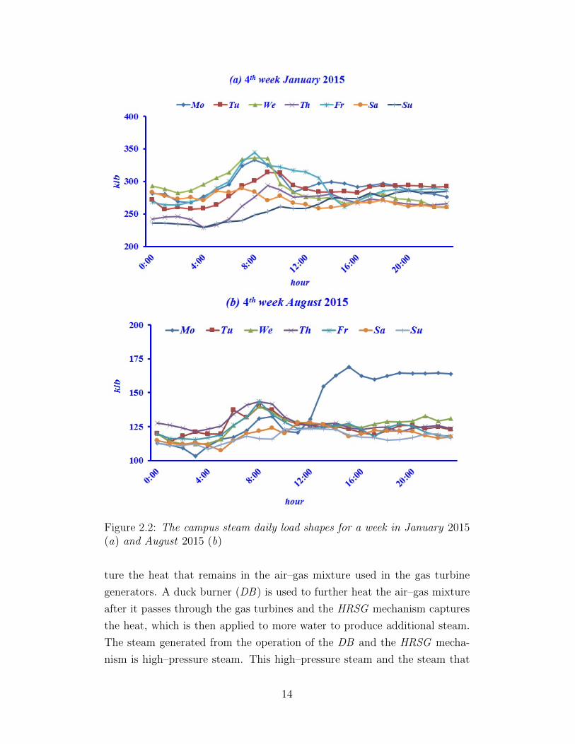
Figure 2.2: The campus steam daily load shapes for a week in January 2015(a) and August 2015 (b)

ture the heat that remains in the air–gas mixture used in the gas turbine

generators. A duck burner (DB) is used to further heat the air–gas mixture

after it passes through the gas turbines and the HRSG mechanism captures

the heat, which is then applied to more water to produce additional steam.

The steam generated from the operation of the DB and the HRSG mecha-

nism is high–pressure steam. This high–pressure steam and the steam that

14

passes through the high–pressure steam turbine generators is expanded to

become low–pressure steam. This low–pressure steam and the steam that

passes through the steam turbines of the low–pressure steam turbine gener-

ators is then distributed to the campus to meet the campus steam load. We

display a schematic of the APP configuration in Figure 2.3. At present, the

APP generates approximately 275,000 MWh annually, roughly 50% of the

total campus annual electricity consumption.

The CUS central chilled water system consists of six chiller plants and

approximately 23 miles of chilled water distribution piping. The vintage of

the chillers ranges from 1993 to 2012. The chiller plants deliver the necessary

chilled water to operate the air conditioning systems in the campus facilities.

Seven chillers with a combined capacity of 27,630 tons are located at the

Oak Street Chiller Plant, seven chillers with a combined capacity of 9,400

tons are located at the North Campus Chiller Plant, four chillers with a

combined capacity of 4,340 tons are located at the Library Chiller Plant,

two chillers with a combined capacity of 2,000 tons are located at the Animal

Science Chiller Plant and three chillers are located at the Chem Life Science

Chiller Plant with a combined capacity of 3,630 tons. In addition, a 6.5

million gallons thermal energy storage tank provides 50,000 ton-hours of

daily cooling capability.

In the 2015 Illinois Climate Action Plan (iCAP), UIUC set a goal that,

by 2020, 12.5 GWh of electricity will be produced by solar installations on

campus property. To meet this goal, UIUC dedicated 20.5 acres (82,961 m2)

of campus land in the South Farms area to allow the construction of the

Phoenix Solar South Farm (PSSF ). UIUC signed a 10-year Power Purchase

Agreement (PPA) with the developer Phoenix Solar Inc. to design, build,

operate and maintain the solar farm for the first 10 years of its life, at

which point the solar farm becomes the property of the University. PSSF

serves to meet the campus electricity load in a clean way. The PSSF is

connected directly to the CUS electrical distribution system. The annual

energy production from the solar farm is estimated to be 7.86 GWh, roughly

2% of the 2012 campus electricity consumption of 432.45 GWh. UIUC has

agreed to purchase all the energy from the solar farm for the first 10 years.

To supplement the outputs of the APP and PSSF, CUS buys electricity

on the MISO market. The purchased electricity is transmitted from the

injection node to a transmission node from which the delivery is made to the

15

Figure 2.3: The schematic of the Abbott power plant layout

Figure 2.4: Phoenix Solar South Farm

16

campus at the Main Substation (MSS ) via the Ameren DN. At present, the

import capacity from the Ameren DN is limited to 60 MW.

The existing CUS electricity distribution grid includes approximately 300

miles of electrical cable. In Figure 2.5, we show the single line diagram of the

CUS electricity distribution grid. This distribution grid is a 3–phase, medium

voltage electricity network connected to the Ameren DN at a single point of

interconnection – the MSS. The MSS is a 69–kV substation which is directly

connected to the South–East Substation (SES ) by s 69–kV distribution line

of the campus distribution grid. The APP is connected to the MSS. There

are 11 load centers (LC s) connected to the two campus substations and the

LC s aggregate all the loads on campus. The UIUC solar farm is connected

to the bus that serves LC 10.

Figure 2.5: Simple single line diagram of the campus electricity grid

The CUS has 30 miles of steam piping throughout the campus. The

CUS steam distribution system consists of two distinct subsystems: campus

pressure system (CPS ) and high pressure system (HPS ). The CPS is the

low–pressure steam system and it is the primary source of heat distribution

to the campus facilities such as some laboratories. The HPS provides the

17

high–pressure steam to a few facilities with steam process loads that require

higher pressure steam.

The CUS also has 23 miles of chilled–water piping on campus. The chilled–

water distribution system consists of underground, direct buried piping con-

structed from concrete pipe and ductile iron pipe. The majority of the piping

has been installed within the past 15 years.

2.2 CUS Operations under the Current Paradigm

The CUS objectives are to provide the chilled water, steam and electricity

services at all times in a reliable and an economic manner under the current

paradigm. In this section, we explain how CUS tries to achieve its objectives.

CUS is an integrated utility system with the three services – chilled water,

steam and electricity – that are strongly inter–dependent. We point out that

we do not discuss the chilled water system as it is a part of the CUS electricity

system. Specifically, the chilled water utility system in the CUS relies entirely

on the CUS electricity system as all the chiller plants that serve the chilled

water demand electricity loads. The steam demand on campus determines

the APP schedules and the electricity generated is thus a by–product of the

APP steam production. The APP schedules, in turn, govern the purchase

decisions on the amounts of electricity bought in the MISO markets to meet

the campus electricity loads. These structural inter–dependencies among the

three CUS utilities are so extensive that even if all the electricity consumption

were supplied by renewable resources, the CUS still needs a certain amount

of cogeneration to meet the campus steam demand. For the same reason, the

CUS cannot buy all its electricity on the MISO markets even if the electricity

is cheaper than APP electricity as APP still must cogenerate steam and

electricity to meet the two CUS steam demands. A division in the university

called UIUC Facilities and Services (F&S ) is responsible for the operation

and maintenance of the CUS. The engineering outfit Fellon–McCord provides

support for the F&S staff in terms of energy market and price information.

This information, together with the daily electricity and steam load forecasts,

is essential to determine the schedules and dispatch levels of the APP units.

At present, the lack of appropriate data, forecasting information and tools

analytically limits the efficiency of the CUS resource schedules. As such,

18

under the current paradigm, opportunities for improvements in economics of

operations may exist under different CUS operational paradigms.

Under the current paradigm, a key characteristic is that the CUS elec-

tricity distribution grid is connected to the Ameren DN at a single point

of interconnection at all times. For the electric system in the CUS, if the

APP units fail then, at present the CUS depends on the MISO wholesale

electricity market and the Ameren DN to supply electricity to meet the cam-

pus electricity load. If the tie line connecting the CUS and the Ameren DN

fails, even if the APP available generation capacity is more than the load,

the CUS does not have the capability to run disconnected from the Ameren

DN due to constraints from a protection as well as control standpoint. As

such, the single point of interconnection of the Ameren DN and the CUS

at MSS does not provide the flexibility to disconnect from the Ameren DN

and operate the CUS as a single islanded system. Unlike electricity provi-

sion, if CUS loses the APP units then CUS also loses the ability to provide

steam for campus heating purposes as CUS cannot buy the steam on any

wholesale market and most facilities on campus do not have the capability

to produce and provide the heat locally at the facility itself. Similar to the

discussion on economics of operations, opportunities for improvements in re-

liability of electricity supply to campus loads may also exist under different

CUS operational paradigms.

The campus has adopted the iCAP to pave the path for UIUC to achieve

carbon neutrality as early as possible but no later than 2050. Some of the

recent goals set in the 2015 iCAP for Fiscal Year (FY ) 2020 include 30%

improvement in energy utilization from FY 2008 level and 30 % reduction

in emissions from energy production from the FY 2008 levels. As such, the

iCAP represents a roadmap to a new, prosperous, and sustainable future for

UIUC.

2.3 UIUC CUS Operations under the µg Framework

With respect to the distribution grid size, a µg is a small power system

containing a cluster of interconnected DERs and loads. Since a µg is a

power system, all the attributes and functions of a large system, such as the

bulk power system, hold. A µg differs from the conventional power system

19

in terms of the coordinated control that the µg exercises on both the supply–

side resources and the demand–side resources. A µg is a power system that

operates in either of its two distinct modes: parallel, also known as grid–

tied mode, or islanded, sometimes called the isolated mode. Due to the

coordinated control over the µg generation as well as load resources, a µg may

be viewed as a time–varying resource embedded in the DN with the ability

to either generate or consume electricity or remain idle with 0 injection /

withdrawal in the isolated mode operations. Under the coordinated control,

a µg may exploit the opportunities to inject electricity into and provide

ancillary services (AS ) to the DN and earn revenues. µg loads may be

classified as either critical loads or non–critical loads. The classification is

essential for supply–demand balance under the islanded mode of operation.

Such features provide added degrees of freedom in the operation of the grid

with the integrated µg. In effect, the µg brings a new paradigm in the

operation of the power systems. A µg not only ensures the reliability of the

electricity supply to its critical loads but also takes full advantage of the DN

when needed or opportune. In addition to the services taken from the grid,

a µg is able to provide new operational degrees of freedom to the grid.

The UIUC energy resources – the APP and the PSSF – may be viewed

as the DERs of the CUS. Based on extensive discussions with UIUC F&S

staff, the classification of the campus electricity load into critical and non–

critical loads is easily established. The six chiller plants in the CUS account

for almost 10 MW of campus electricity load and, based on the discussions

with UIUC F&S staff, the chiller plant load may considered a non–critical

load. The campus grid forms an interconnected network of DERs and loads.

As a MISO wholesale electricity market participant, UIUC CUS has the

option to earn revenues for the sale of electricity and also has the option to

exploit the opportunities for AS provision to the bulk grid in the MISO AS

market. With the way UIUC CUS is connected to the Ameren DN, it has

a defined geographical boundary in the Ameren DN footprint. Except for a

few structural features, the UIUC CUS has all the required characteristics

of a µg and fits the definition of a µg as it has the DERs in the form of the

APP and the PSSF, critical and non–critical loads and a defined electrical

grid boundary. Thus, we may view the CUS as a µg along with associated or

required structural changes.2 In Figure 2.6, we show a transformation of the

2Some of the key structural changes include the requirement of a flexible and a control-

20

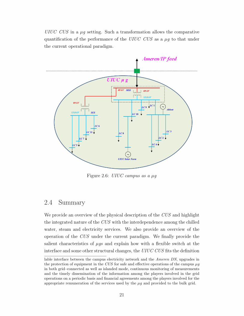
UIUC CUS in a µg setting. Such a transformation allows the comparative

quantification of the performance of the UIUC CUS as a µg to that under

the current operational paradigm.

Figure 2.6: UIUC campus as a µg

2.4 Summary

We provide an overview of the physical description of the CUS and highlight

the integrated nature of the CUS with the interdependence among the chilled

water, steam and electricity services. We also provide an overview of the

operation of the CUS under the current paradigm. We finally provide the

salient characteristics of µgs and explain how with a flexible switch at the

interface and some other structural changes, the UIUC CUS fits the definition

lable interface between the campus electricity network and the Ameren DN, upgrades inthe protection of equipment in the CUS for safe and effective operations of the campus µgin both grid–connected as well as islanded mode, continuous monitoring of measurementsand the timely dissemination of the information among the players involved in the gridoperations on a periodic basis and financial agreements among the players involved for theappropriate remuneration of the services used by the µg and provided to the bulk grid.

21

of a µg. The µg concept application to the UIUC CUS forms the basis of

the work described in this thesis. We make extensive use of the information

provided in this chapter about the UIUC CUS energy resources and the

distribution grid to model and emulate the CUS operations under different

paradigms.

22

CHAPTER 3

METHODOLOGY FOR THEQUANTIFICATION OF THE CUSOPERATIONAL PERFORMANCE

In this chapter, we describe in detail the methodology we deploy to quan-

tify the operational performance of the CUS. We start out with a discussion

of the quantification needs and requirements for the systematic and compre-

hensive quantification of the operational performance of the CUS under both

the optimal operations of the current and the µg operational paradigm. We

then provide the simulation approach. We lay out the basic time frame of

the simulation and proceed to provide an overview of the MCS we perform

to emulate the CUS operations. We outline the comprehensive simulation

methodology that provides the capability to quantify the impacts of CUS

operations on the economic, reliability and emissions of the CUS. We dis-

cuss the formulation of the energy scheduling optimization problem (ESOP)

whose solution forms an essential element in our quantification methodology.

The ESOP solution determines the schedule of the APP energy resources

under the optimal operations of the current operational paradigm which is

used as a proxy for the current operational paradigm. The current approach

to schedule the energy resources does not involve any analytical optimization

techniques, and the proposed ESOP solution replaces the current heuristic–

based approach to determine the schedule and loading levels of the APP

energy resources. A modified ESOP and its solution is also adopted for

the quantification of the CUS operational performance under the µg opera-

tional paradigm. We provide the detailed description and report the use of

the simulation methodology we adopt to quantify the CUS operational per-

formance. This chapter devotes a section to the discussion of the metrics of

interest and the details for their evaluation from the simulation outputs. The

simulation methodology and evaluation of the metrics constitute important

contributions of this work.

23

3.1 Quantification Methodology Overview

We discuss here the quantification needs that must be met by the method-

ology we propose such that it is systematic and comprehensive enough to

allow us to make engineering judgments over the operational performance

of the CUS. We wish to provide the figures of merit for metrics of inter-

est to assess the economics, reliability and the environmental impacts of the

CUS operations so as to allow the meaningful comparison of the CUS op-

erational performance under the optimal operations of the current and the

µg operational paradigm on a consistent basis. We wish to adopt a method-

ology that can comprehensively quantify the CUS operational performance

for any specified duration so as to explicitly take into account the seasonal

impacts on the operational performance of the CUS. Our approach must no-

tably be able to represent all the salient features of CUS operations. The

methodology should take into account the uncertainties and time varying

phenomena in the operations of a system like the CUS be able to quantify

the CUS operational performance under the optimal operations of the cur-

rent and the µg operational paradigm on the basis of appropriate metrics

which would allow the comparative assessments on the benefits of the µg

concept application to the UIUC CUS. In addition, we wish to understand

the impacts on the CUS operational performance by answering the various

“what if ” questions including what if there is a change in the resource mix,

maintenance schedules in the operation of the CUS, change in the policy etc.

The CUS operations in any hour involve time varying phenomena in terms

of the campus steam and electricity load, PSSF generation output and un-

certainties with respect to the availability of the APP conventional energy

resources and the electricity network. A system like the CUS involves many

stochastic or random elements and therefore it defies any analytic study. As

such, there exists no closed form analytical expression that can provide the

figures of merit for the metrics on economics, reliability and emissions of

the CUS operations while also taking into account uncertainties and time

varying phenomena involved in the CUS operations. Therefore, we require a

systematic simulation methodology which can comprehensively quantify the

CUS operational performance while addressing all the quantification needs.

Simulation in a narrow sense is the experimentation with a system over time

and it provides the ability to sample the values of the stochastic elements

24

and study their impacts over time on the CUS. The simulation also allows

the investigation of the behavior of the CUS over time thereby taking into

account the seasonal impacts and changes in the policies. The CUS is a

complex system since each element in the system influences the behavior

of other systems and therefore simulation is useful for capturing the com-

plexities of the CUS operations. The conventional probabilistic simulation

approach [22],[23] cannot adequately provide the needed level of detail due

to its inability to represent chronological phenomena such as the CUS oper-

ations as well as the time dependent nature of the CUS steam and electricity

load and energy supply resources, particularly the PSSF. A distinctly dif-

ferent approach, which may be used to represent uncertain CUS operations,

with the capability represent all the constraints, is the probabilistic optimal

power flow (P–OPF ),[24]. One drawback of the P–OPF approach, however,

is that it requires a number of significant simplifying assumptions to render

the problem into a solvable form. For instance, the representation of the

CUS operations over time, including the temporal correlations among the

system variables, requires the formulation of a multi–period P–OPF, whose

tractability is questionable even for small number of periods. Many renew-

able integration studies in the literature report the use of the Monte Carlo

simulation to represent the power system and its sources of uncertainty in

a given period [25]. However, many such papers do not provide the explicit

description of the extension to multiple periods.

We provide the overview of the comprehensive simulation methodology

that can provide the capability to quantify the impacts of the µg concept ap-

plication to the CUS and compare it with the CUS operational performance

under the optimal operations of the current operational paradigm. Our sim-

ulation makes use of the MCS techniques and extends them to multiple time

periods to overcome the limitations of the other simulation techniques dis-

cussed above. As such, the simulation is carried out for a given study period

T that may range, typically, from a few weeks to multiple years. We decom-

pose the study period T into non–overlapping simulation periods Ti with

T =⋃Ti=1 Ti with Ti ∩ Tj = φ, i 6= j. We define each simulation period Ti

in such a way that the CUS resource mix, unit commitment, the market

structure in which the campus participates and the seasonal effects remain

unchanged over its duration. Given the nature of the UIUC CUS demands

and the operations of its resources we use a day as the simulation period. We

25

further decompose each simulation period into subperiods, where a subperiod

is the smallest indecomposable unit of time represented in the simulation. We

assume that each variable remains fixed over the entire subperiod duration.

The simulation, as such, cannot represent any phenomenon whose time scale

is shorter than a subperiod. We choose to use subperiods of one hour du-

ration. We denote by h the index of the subperiods in a simulation period

Ti = {h : h = 1, 2, ..., 24}. We graphically depict the time frame used for the

simulation in Figure 3.1.

Figure 3.1: The time frame used in simulation approach with the subperiodsof a simulation period Ti indicated

We note that we run the MCS for each simulation period Ti. We treat each

simulation period Ti as independent of another simulation period Tj, i 6= j.

As such, the outcome of the MCS of a given simulation period has no bearing

on the Monte Carlo simulation of any other simulation period, and so each

simulation period is simulated independently from the others. We describe

the MCS of an arbitrary simulation period Ti.The simulation emulates the CUS operations in a given simulation period

Ti. The starting point in the emulation is to determine the scheduling of the

CUS resources for the 24 hours of the simulation period. For this purpose,

we need to perform the modeling of the variable campus load, the conven-

tional resource available capacity for each boiler and the generator and the

PSSF generation output used in our simulation approach. Each variable is

uncertain and we represent it in the terms of a discrete-time random process

(r.p.), i.e., a collection of random variables (r.v.s) indexed by the 24 hours

in the simulation period. Such a model of the load, available capacity and

renewable resource output is well explained in detail in [26] and we adopt the

26

notation and the framework developed in that report. We view r.p.s as the

inputs in the simulation, in the sense that their multi–period realizations,

the so–called sample paths (s.p.s), determine the inputs to the 24 scheduling

problems of the simulation period for the CUS. For convenience in the rest

of the thesis, we refer to these r.p.s as input r.p.s.

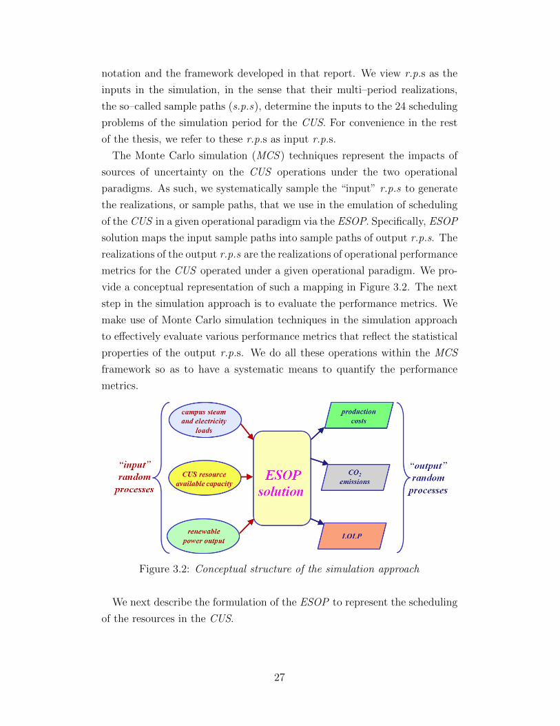
The Monte Carlo simulation (MCS ) techniques represent the impacts of

sources of uncertainty on the CUS operations under the two operational

paradigms. As such, we systematically sample the “input” r.p.s to generate

the realizations, or sample paths, that we use in the emulation of scheduling

of the CUS in a given operational paradigm via the ESOP. Specifically, ESOP

solution maps the input sample paths into sample paths of output r.p.s. The

realizations of the output r.p.s are the realizations of operational performance

metrics for the CUS operated under a given operational paradigm. We pro-

vide a conceptual representation of such a mapping in Figure 3.2. The next

step in the simulation approach is to evaluate the performance metrics. We

make use of Monte Carlo simulation techniques in the simulation approach

to effectively evaluate various performance metrics that reflect the statistical

properties of the output r.p.s. We do all these operations within the MCS

framework so as to have a systematic means to quantify the performance

metrics.

Figure 3.2: Conceptual structure of the simulation approach

We next describe the formulation of the ESOP to represent the scheduling

of the resources in the CUS.

27

3.2 ESOP

The CUS scheduling involves two commodities – steam and electricity –

and its objective is to optimize the combined production costs of the two

commodities. For the formulation of the CUS scheduling problem, we incor-

porate the inter–dependencies involved between the two commodities. We

formulate the CUS scheduling problem to determine the most economic oper-

ational trajectory for the CUS energy resources considering the demands, the

output of the PSSF and the available capacity of each energy resource during

the simulation period. The solution of this optimization problem determines

CUS energy resource schedule of each controllable unit, for each hour of the

optimization period H = {h : h = 1, ..., H}. The optimization period H

represents the duration of each simulation period Ti. The CUS scheduling

problem is formulated as a multi–period optimal power flow (OPF ) problem

with explicit representation of the physical limits of the boilers, generators

and electricity distribution lines. In the formulation, we assume lossless net-

work – the usual condition in the linearized power flow model.

For the scheduling problem formulation, we introduce the following nota-

tion. We use N = {n : n = 1, ..., N} to denote the set of electricity grid

nodal indices with 0 being the index for the slack bus and L = {` : ` =

1, ..., L} to be the set of the electricity distribution line indices. The matri-

ces A,B d and B denote the reduced branch–to–node incidence, the branch

susceptance and the reduced nodal susceptance matrices, respectively. We

denote by b 0 the column vector of the augmented susceptance matrix corre-

sponding to the slack node and by θ the vector of voltage phase angles at the

|N | − 1 buses in N except the slack bus. We denote by f [h] = B d A θ[h]

the vector of line flows in hour h.

We denote by B = {b : b = b1, b2, ..., bB} the set of CUS boilers, with

B ∨(B ∧) the subset of low–pressure(high–pressure) boilers, with B =

B ∨⋃B ∧. For simplicity in the formulation, we treat the operation of

the duck burners similarly to that of the high–pressure boilers and so there

is no explicit representation of the duck burners. We denote by G = {g : g =

σ1, σ2, ..., σS, γ1, γ2, ..., γG} the set of controllable CUS generators. G σ(G γ)

denotes the subset of steam(gas) turbine generators, with G = G σ⋃

G γ.

G σ∨(G σ∧

) denotes the subset of steam turbine generators that work on

low–pressure(high–pressure) steam, with G σ = G σ∨ ⋃G σ∧

. We denote

28

the total steam demand or consumption of campus in hour h as s d[h]. We

denote the efficiency in steam distribution to the campus as η s and so the

CUS net steam production denoted by s p[h] in hour h is 1η s ·s d[h]. For hour

h, we denote by s b[h] the steam generated by a boiler b ∈ B. We denote

the steam produced due to HRSG mechanism in any hour as a constant s ρ.

We denote load in hour h at electricity grid node n by p dn[h]. This hourly

nodal load variable is assumed to be a constant fraction δ n of the hourly

total CUS electricity load d[h] and so p dn[h] = δ n.d[h] for each node n ∈ N .

We denote the conventional generation power injection in hour h by p cn[h]

and the renewable generation injection in hour h by p rn[h]. We denote

the electricity power output by a gas turbine generator g ∈ G γ by p g[h].

Analogously, we denote the hour h power output by the low–pressure (high–

pressure) steam turbine generators by p G σ∨[h](p G σ

∧[h]). In equation (3.1),

we define p G σ∨[h] as the product of the low–pressure steam production rate in

klb/h of the low–pressure boilers in hour h and a conversion factor of hourly

rate of low pressure steam into hourly electricity power output (kWh/h)

denoted by κ ∨.

p G σ∨

[h] = κ ∨.∑b∈B ∨

s b[h] (3.1)

Similarly in equation 3.2, we define the p G σ∧[h].

p G σ∧

[h] = κ ∧.[ ∑b∈B ∧

s b[h] + s ρ]

(3.2)

We denote the electricity imported (exported) from (to) the wholesale

electricity market by p i[h](p e[h]). Note that for each hour h ∈H , at most

one variable between p i[h] and p e[h] may have a non–zero value. Any other

notational detail left unmentioned here is given in Appendix B.

The CUS scheduling objective is to meet the campus electric and steam

loads at the least production costs. In words, the objective function mini-

mizes the production cost of electricity and steam required by the campus

where the electricity costs are represented by the costs incurred due to the

operation of the gas turbine generators and the electricity imported from or

exported to the wholesale electricity market and the steam costs are repre-

sented by the costs incurred due to the operation of the boilers. We do not

consider the cost functions associated with the electricity generated from the

29

steam turbine generators because of the integrated nature of our problem.

The requirement to meet the steam load governs and drives the operation

of the APP and we consider the costs incurred in the production of the

steam and get the electricity generated from the steam turbine generators as

a byproduct of the steam generation in the problem formulation. We point

out that based on the data available, the cost functions are assumed to be

linear functions. The decision variables for the production cost minimization

problem are the steam s b[h] produced by each boiler b ∈ B, the power out-

put p g[h] by each gas turbine generator g ∈ G γ and the power p i[h](p e[h])

imported (exported) from (to) the wholesale electricity market ∀h ∈H . We

state the minimization objective as:

mins b[h],p g [h],p i[h],p e[h]

∑h∈H

[∑b∈B

c b(s b[h])+∑g∈G γ

c g(p g[h])+c i(p i[h])−c e(p e[h])]

(3.3)

The objective is subject to various physical and operational constraints.

We consider the steam balance constraint. The hourly steam produced by

the HRSG mechanism and all the boilers must equal the hourly total CUS

steam load as seen which is the hourly steam demand or consumption of the

campus divided by the steam distribution efficiency. We denote by µ[h] the

dual variable associated with the steam load balance constrain represents the

marginal cost of providing steam. We present the steam balance constraint

in equation (3.4).

µ[h] ↔∑b∈B

s b[h] + s ρ =1

η s(s d[h]) ∀h ∈H (3.4)

For the electricity load balance, we require the nodal power injection1 to

exactly match the nodal load at each electricity grid node, including the

slack node. We make use of p c[h] in the electricity load balance constraints

to represent the vector of conventional electricity generation on each node

with the exception of the slack node of the electricity network. p c0[h] is

1For the CUS electricity network, in addition to the slack node where the APP isconnected, the conventional electricity injection is only at the node which is connectedto the Ameren DN in the hours when the campus imports electricity from the wholesalemarket. This interconnection node may also be an electricity withdrawal node wheneverCUS sells electricity to the upstream network and for this node, the conventional powerinjection or withdrawal will just be p i[h] or p e[h].

30

the electricity injection at the slack bus. For the CUS, p c0[h] represents the

electricity generated from the steam and gas turbine generators of the APP.

Mathematically, p c0[h] = p G σ

∨[h] + p G σ

∧[h] +

∑g∈G γ p g[h]. We denote by

λ n[h] the marginal cost of providing electricity at CUS electricity network

node n in hour h respectively. We denote λ[h] as the vector of λ n[h] at

the |N | − 1 nodes in N except the slack bus. We denote by λ 0[h] the

marginal cost of providing electricity at the slack node. We state electricity

load balance constraints in terms of the so–called DC power flow equations

as:

λ[h] ↔ p c[h] + p r[h]− p d[h] = B θ[h], ∀h ∈H (3.5a)

λ 0[h] ↔ p c0[h] + p r

0[h]− p d0[h] = b †0 θ[h], ∀h ∈H (3.5b)

In addition, we must explicitly incorporate the electricity distribution line

constraints to ensure that no electricity grid line flow violates its thermal

limits:

f m[h] ≤ f [h] ≤ f M[h] ∀h ∈H (3.6)

The consideration of the various physical limits on the electricity and steam

generation units in the campus grid results in additional constraints. We

denote the sum of the maximum available capacity of each low–pressure(high-

pressure) steam turbine generator by (p G σ∨[h])M((p G σ

∧[h])M). We state

physical limit constraints as shown below.

0 ≤ s b[h] ≤ (s b[h])M , ∀h ∈H , ∀b ∈ B (3.7)

0 ≤ p g[h] ≤ (p g[h])M , ∀h ∈H , ∀g ∈ G γ (3.8)

0 ≤ p G σ∨

[h] ≤ (p G σ∨

[h])M , ∀h ∈H (3.9)

0 ≤ p G σ∧

[h] ≤ (p G σ∧

[h])M , ∀h ∈H (3.10)

Additional constraints arise from the limits on the import (export) of power

from (to) the MISO wholesale electricity market via the Ameren DN in hour

h which we represent in equations below.

31

0 ≤ p i[h] ≤ (p i)M , ∀h ∈H (3.11)

0 ≤ p e[h] ≤ (p e)M , ∀h ∈H (3.12)

We summarize the CUS scheduling objective and the constraints as follows:

mins b[h],p g [h],p i[h],p e[h]

∑h∈H

[∑b∈B

c b(s b[h]) +∑g∈G γ

c g(p g[h]) + c i(p i[h])− c e(p e[h])]

subject to

∑b∈B

s b[h] + s ρ =1

η s(s d[h]) ∀h ∈H (3.13a)

p c[h] + p r[h]− p d[h] = B θ[h], ∀h ∈H (3.13b)

p c0[h] + p r

0[h]− p d0[h] = b †0 θ[h], ∀h ∈H (3.13c)

f m[h] ≤ f [h] ≤ f M[h] ∀h ∈H (3.13d)

0 ≤ s b[h] ≤ (s b[h])M , ∀h ∈H , ∀b ∈ B (3.13e)

0 ≤ p g[h] ≤ (p g[h])M , ∀h ∈H , ∀g ∈ G γ (3.13f)

0 ≤ p G σ∨

[h] ≤ (p G σ∨

[h])M , ∀h ∈H (3.13g)

0 ≤ p G σ∧

[h] ≤ (p G σ∧

[h])M , ∀h ∈H (3.13h)

0 ≤ p i[h] ≤ (p i)M , ∀h ∈H (3.13i)

0 ≤ p e[h] ≤ (p e)M , ∀h ∈H (3.13j)

The CUS scheduling problem defined by the objective function and the

constraints defined in the equations (3.13a)–(3.13j) constitute a large–scale

linear programming (LP) problem and provide the mathematical statements

for the so–called ESOP. The ESOP represents the mathematical formulation

of the real world problem of scheduling of the CUS energy resources with

optimal energy production costs under all conditions. The ESOP is a deter-

ministic problem whose solution determines the schedule of the CUS energy

resources in each hour h ∈ H . ESOP consists of h separate OPF problems

where each OPF problem represents the scheduling problem in each hour h

∈ H . We use the sampled realizations such as d[h] of the CUS electricity

load demand input r.p., s d[h] of the CUS steam demand input r.p., p r[h]

32

of the renewable resource generation input r.p. and (s b[h])M , (p g[h])M ,

(p G σ∨[h])M , (p G σ

∧[h])M , (p i)M and (p e)M of the resource available ca-

pacity input r.p.s are used as the ESOP parameters. The ESOP may be

solved by any standard LP solver. The optimal solution of the ESOP also

give results for the dual variables associated with the various constraints in

the ESOP. Of importance are the dual variables associated with the steam

load balance equation (3.4) and the dual variables associated with electric

power balance equations (3.5a) and (3.5b). Ideally, the CUS resources must

be scheduled the way ESOP is described but due to the lack of appropri-

ate data, forecasting information and tools, the CUS resources scheduling is

based on heuristics. The ESOP developed represents the scheduling problem

of the CUS resources in the optimal operations of the current operational

paradigm.

For the quantitative comparison, we adopt a modified ESOP which will

represent the scheduling problem of the CUS resources in the µg operational

paradigm. To convert the above ESOP so as to be able to emulate the

scheduling problem of the CUS operations as a µg, we make a few mod-

ification to the problem formulation. These modifications are necessary to

accommodate the two modes of operation that a µg can operate in. Under the

µg operational paradigm, for the CUS µg operations in the grid–connected

mode, the ESOP statement remains exactly identical to the equations defined

in (3.13). However, under the islanded mode operations, we use a modified

formulation of the ESOP. For the islanded–mode operations, we remove both

the decision variable p i[h] and p e[h] due to their associated zero values. The

resulting ESOP can then represent the scheduling problem of the CUS µg

resources in the islanded mode. Under the µg operational paradigm, to em-

ulate the scheduling problem of the campus grid resources when operated as

µg, we switch between the ESOP defined in equation (3.13) and the modified

ESOP that we define in equations (3.14).

mins b[h],p g [h],p i[h],p e[h]

∑h∈H

[∑b∈B

c b(s b[h]) +∑g∈G γ

c g(p g[h])]

33

subject to

∑b∈B

s b[h] + s ρ =1

η s(s d[h]) ∀h ∈H (3.14a)

p c[h] + p r[h]− p d[h] = B θ[h], ∀h ∈H (3.14b)

p c0[h] + p r

0[h]− p d0[h] = b †0 θ[h], ∀h ∈H (3.14c)

f m[h] ≤ f [h] ≤ f M[h] ∀h ∈H (3.14d)

0 ≤ s b[h] ≤ (s b[h])M , ∀h ∈H , ∀b ∈ B (3.14e)

0 ≤ p g[h] ≤ (p g[h])M , ∀h ∈H , ∀g ∈ G γ (3.14f)

0 ≤ p G σ∨

[h] ≤ (p G σ∨

[h])M , ∀h ∈H (3.14g)

0 ≤ p G σ∧

[h] ≤ (p G σ∧

[h])M , ∀h ∈H (3.14h)

The switch between the ESOP and the modified ESOP defined in equa-

tions (3.13) and (3.14) depends upon the mode of operation of the UIUC CUS

µg among the different hours of the optimization period H . For the UIUC

CUS, this switch would occur whenever there is an outage in the upstream

grid and the UIUC CUS islands its DERs and loads to maintain the continu-

ity of electricity supply. The UIUC CUS switches back to the grid–connected

mode of operations as the supply of electricity in the upstream network is

brought back. We describe the modified ESOP for islanded–mode operations

below.

The ESOP described in this section forms a key component of the sim-

ulation methodology for the quantification of the operational performance

of the CUS under the optimal operations of the current as well as the µg

operational paradigm.

3.3 Simulation Methodology Description

We note that we describe the application of the simulation methodology

to a single specified period and the application of the methodology on any

other simulation period is analogous. We make extensive use of the MCS

techniques in the simulation methodology. We provide in Figure 3.3 a con-

ceptual flow chart of the overall MCS procedure and proceed to formally

describe it in what follows.

34

Figure 3.3: Monte Carlo simulation: conceptual flow chart

The simulation approach makes use of the so–called independent Monte

Carlo [20] and requires the construction of multiple independent and iden-

tically distributed (i.i.d.) s.p.s for each output r.p. to evaluate the perfor-

mance metrics. Note that the phrase “i.i.d. s.p.s” has the sense that the

s.p.s constitute the realizations of independent identically distributed r.p.s.

A simulation run is the basic process through which we construct a s.p. for

each of the output r.p.s. In each simulation run, we sample each input r.p.

in order to generate the s.p.s. The s.p.s of the input r.p.s are mapped via

the ESOP solution into the s.p.s of all the output r.p.s. Thus each execution

of the simulation run results in an additional s.p. of each output r.p.. We

carry out M simulation runs with M = m and m provide the number of MC

runs used in order to create the output s.p.s from which we estimate the per-

formance metrics of interest. The number of simulation runs M depends on

the statistical reliability specified for the estimation of the desired expected

values. The idea behind the statistical reliability is to ensure that the sam-

ple mean estimate is within a certain specified confidence interval of the true

mean of the output r.p.s . The length of the confidence interval is a function

of M − 12 [20]. While it is possible to select M so as to set the confidence

interval length and achieve the desired statistical reliability, in practice, a

function in M − 12 decays very slowly for large M , so the improvement in sta-

tistical reliability is too small to warrant the extra computing–time needed

to perform additional simulation runs.

35

3.4 Evaluation of Performance Metrics

We select our performance metrics to be the expected values of the time-

indexed r.v.s making up the output r.p.s of interest. Let M be the number

of simulation runs; we estimate, for an output r.p. Y˜ [h] : h = 1, ..., 24, the

hourly sample mean point estimate y[h] of each r.v. Y˜ [h], h = 1, ..., 24:

y[h] =1

M

M∑j=1

y(j)[h] (3.15)

where y(m)[h] is the realization of r.v. Y˜ (m)[h] in simulation run m.

We now focus on an independent simulation run m and analyze it to even-

tually explain the approach taken in the simulation to effectively evaluate

the various performance metrics. The optimal solution to the ESOP in each

independent simulation run m yields, for each hour h, the optimal schedule

of the CUS resources in the campus grid, i.e., the boiler output (s b[h])∗ of

each boiler b ∈ B, the power output (p g[h])∗ of each gas turbine generator

g ∈ G γ, the power imported(exported) (p i[h])∗((p e[h])∗), the marginal cost

to provide an additional klb of steam to campus (µ[h]) ∗ and the marginal

costs to provide an additional kWh of supply (λn[h]) ∗ at each CUS electric-

ity network node n in hour h. We now make use of these optimal outcomes

in each hour h from the simulation run m to evaluate the hourly values of

the s.p.s for the output r.p.s of interest.

The total production costs c[h] in hour h are computed as:

c[h] =∑b∈B

c b((s b)∗[h]) +∑g∈G γ

c g((p g)∗[h]) + c i((p i)∗[h])− c e((p e)∗[h])

(3.16)

and the total production costs over the period H is then given by∑

h∈H c[h].

We also are interested in emission metrics. For that purpose we compute

the indices χ b, the quantity of CO2 emissions in metric tons/klb released

by the operation of boiler b ∈ B and χ g, the quantity of CO2 emissions in

metric tons/kWh released by the operation of gas turbine generator g ∈ G γ.

Then, the total hour h CO2 emissions are given by:

v[h] =∑b∈B

χ b.(s b)∗[h] +∑g∈G γ

χ g.(p g)∗[h] (3.17)

36

and the total emissions over the period H is then given by∑

h∈H v[h].

In the case of the reliability metrics, we note that a loss of load event

occurs whenever the electric load is not met. For the case when the CUS is

operated in an optimized paradigm, we note that a loss of load event occurs

due to a supply shortfall or due to the failure of the tie line that connects

the CUS to the Ameren DN. For the case when the CUS is operated in a

µg paradigm, the loss of load event occurs when there is a supply shortfall

in the grid-connected mode of operation. In the islanded mode of the CUS

operations as a µg, the loss of load occurs when there is a supply shortfall

to meet the CUS critical loads. The expected unserved energy in hour h is

the shortfall in supply when the total campus electricity load is not met. Let

u[h] be the unserved energy in hour h and its value is computed as:

We use the indicator function i(o,+∞)(·) to compute the system LOLP con-

tribution in hour h. We define the indicator function i(o,+∞)(·) as follows:

i(o,+∞)(x) =

1 x 6= 0

0 otherwise

The function takes for argument the unserved energy in hour h and returns

1 whenever the unserved energy is positive, 0 otherwise. Then, the system

LOLP contribution in hour h is given by i(o,+∞)(u[h]).

To conclude this section, we stress that all the hourly realizations obtained

as above, together with hourly realizations of other subperiods, constitute

s.p.s of their associated output r.p.s. With each simulation run (m), a set of

new s.p.s of the output r.p.s is obtained and used to evaluate the performance

metrics of interest via equation (3.15). The evaluation of the performance

metrics of interest for the given simulation period concludes the MCS of

the simulation period. We can carry out the simulation of other simulation

periods in a similar way.

3.5 Summary

The chapter discusses the requirements from a systematic simulation method-

ology to quantify the CUS operational performance and describes the devel-

opment of the quantification approach. We discuss the development of a key

37

component of the simulation methodology which is the ESOP. An important

part of this chapter was the modifications made in the ESOP formulation

with the changes from the optimal operations of the current to the µg oper-

ational paradigm. The methodology is simple and can be easily adapted to

any other power system. The methodology provides the means to quantify

the operational performance of the CUS over longer duration under the two

operational paradigms and enables us to carry out the quantitative compar-

ison.

38

CHAPTER 4

QUANTIFICATION STUDIES

The µg concept leads to a new paradigm to operate the power system with

the promise of numerous benefits. In our earlier discussions, we noted that

the literature provides an adequate description of the µg benefits but there

remains a need to systematically quantify such benefits so as to justify in-

vestments to the µg projects. Thus, we aim to see the extent to which the

potential µg benefits can accrue to a power network when operated as a

µg. For the CUS, we conceptually transform the UIUC CUS into a µg and

evaluate via simulation its expected production costs, LOLP and emissions

and compare them to those under the current operational paradigm so as

to understand the realized benefits for operations under the µg operational

paradigm. Formally, we assess the extent to which the highly touted ben-

efits of a µg can be realized in the case of the UIUC CUS operated as a

µg. We make use of the optimization techniques in the scheduling problem

and the way we approach the use of optimization is to allow the meaningful

comparison of current versus the µg operational paradigm. Since µg oper-

ations involve optimization, we compare the operational performance under

the optimal operations of the current paradigm and the µg paradigm. We do

provide the historical data to show how close heuristics based operation in the

current operational paradigm is to the results attainable under the optimal

operations of the current operational paradigm. This side–by–side compara-

tive assessment of the operational performance of the UIUC CUS operation

under a µg operational paradigm and optimal operations of the current oper-

ational paradigm provides a quantification of the relative economic, reliability

and environmental performance results under the two paradigms. We stress

that, given the critical importance of the steam load and its impact on the

operations of the electricity supply resources, this application of the µg op-

erational paradigm to the UIUC CUS is quite distinct from the applications

discussed in the literature. We shall point out the differences in our discus-

39

sion of the interpretation of the study results. Our comparative assessment

idea is illustrated by Figure 4.1.

Figure 4.1: Side–by–side comparison of the reliability of electricity supply,emissions and economics metrics for the CUS operations under the twooperational paradigms

In this chapter, we deploy the simulation approach presented in chapter 3

to obtain the results of the UIUC CUS operations under the µg and the op-

timal operations of the current paradigm. The results provide useful insights

into the quantification of the relative benefits of the µg concept application

in terms of the economics, reliability and emission indices with respect to the

UIUC CUS operations under the current and µg operations. The compar-

ative quantification study is particularly useful to understand the impacts

of the solar energy with the existing fossil fuel units in the CUS under the

two paradigms. We include a detailed interpretation of the results so as to

understand all the ramifications of operations under the µg paradigm.

We begin with an overview of the data used in the study we present. We

discuss the scope and the nature of the studies. We next present the results in

the subsequent sections and discuss the findings and provide the insights into

the comparative advantages of µg operations relative to operations under the

optimal operations of the current paradigm. We summarize the chapter in

the final section.

40

4.1 Overview of the Study

We applied the proposed simulation methodology to the UIUC CUS to

carry out a study under both the optimal operations of the current and

µg paradigm and evaluated all metrics of interest. The study helps under-

stand the extent to which the µg benefits are realized when a power system

such as the UIUC CUS is operated as a µg. The study is done on two cases,

namely the base case and the PSSF case.

In the base case, we compare the CUS operational performance for the

optimal operations of the current and the µg operational paradigm on the

basis of the average daily cost of energy production in dollars as the metric

for economics, average daily LOLP as the metric for reliability and average

daily CO2 emissions in metric tons as the metric of emissions. The PSSF

case includes the UIUC PSSF in the CUS resource mix and provides a similar

comparison of the CUS operational performance for the optimal operations

of the current and µg operational paradigm on the basis of the same metrics

of interest. We interpret the results obtained from each case independently

and compare the results between the two cases. Such a comparison allows us

to understand the impacts of the PSSF on the performance of CUS under

the two paradigms. We point out that the comparative performance results

obtained in each case are consistent in a sense that the resource mix is held

constant when CUS operational performance is compared under the two

operational paradigms.

For each case, namely base and PSSF, we limit our analysis to a single

year with the 365 days in the year partitioned into four seasons of three

months each and focus on the insights into the nature of the results ob-

tained. Therefore, the four seasons are Jan–Mar, Apr–Jun, Jul–Sep and

Oct–Dec respectively. Taking into account the seasonal effects, maintenance

schedules for the APP conventional resources and the academic calendar of

the university, we select 32 representative days, 8 for each season in the year

as the simulation periods to quantify the CUS operational performance un-

der optimal operations of the current and µg operational paradigm in each

case. We also note that all graphs in both the case studies are done over

the “average day in a season in the year”, for which the hourly values are

averaged over all the representative days, with weights equal to the number

of actual days represented by each representative day. For UIUC CUS test

41

Table 4.1: Electricity and load data

loadJan-Mar Apr-Jun Jul-Sep Oct-Decmin max min max min max min max

electricity (kW) 34 62 37 78 44 81 38 76steam (klb) 150 553 81 227 86 210 130 510

Table 4.2: Electricity resource capacity

electricity resourcemax capacity

(kW)steam generator 1 3.0steam generator 2 3.0steam generator 3 3.0steam generator 4 3.0steam generator 5 7.5steam generator 6 7.5steam generator 7 12.5steam generator 8 12.5steam generator 9 7.0gas generator 1 15.0gas generator 2 15.0

system, our studies indicate that beyond 1000 simulation runs, there is too

little improvement in the statistical reliability of the economic and emission

metrics to warrant the extra computing time required for the execution of

additional simulations runs. For the reliability metric 1300 simulation runs

were required.

The study performed uses the electricity and steam load data for the year

2014 and 2015 provided by the UIUC F&S. The annual peak electricity load

is 81 MW and the annual CUS peak steam load is about 553 klb. We

summarize the electricity and steam load in Table 4.1. The electricity loads

during the Jul–Sep months are higher than the other seasons in an year and

the steam load are higher for the Jan–Mar months.

The total nameplate capacity of the conventional electricity generation

resources is about 89 MW. The CUS can further buy up to 60 MW of

electricity on the MISO wholesale electricity market. The maximum steam

that the APP resources can produce is 624 klb. The maximum individual

APP electricity and steam resource capacities are summarized in Table 4.2

and 4.3.

42

Table 4.3: Steam resource capacity

steam resourcemax capacity

(klb)boiler 1 140boiler 2 110boiler 3 80boiler 4 80boiler 5 80

duck burner 50HRSG 84

Each electricity conventional generator is modeled as a two state unit with

its own failure/recovery rate. The steam producing resources are also mod-

eled as two state units with their own failure/recovery rates. In modeling

conventional electricity and steam generation units, we specifically take into

account the maintenance schedules. The maintenance typically happens dur-

ing September and October. The tie line connecting the UIUC CUS elec-

tricity grid to the Ameren DN is also modeled as a two state unit. For the

PSSF case, we incorporate the UIUC PSSF with a name plate capacity of

4.68 MW. We use the UIUC PSSF data for the year 2016.

There are certain assumptions with respect to the studies performed. The

studies performed are of a backcasting nature. As such, we assume perfect

information about the forecasts since we make use of historical data in our

simulation. To transform the current paradigm into either the optimal oper-

ations of the current or the µg operational paradigm some, asset investments

would have to be made and we assume such investments and do not consider

them in the comparative quantitative analysis.

4.2 Comparison of the CUS Operational Performance

for the Base and PSSF Case

In this section, we present the comparison of the CUS operational perfor-

mance mainly under the two operational paradigms, namely the optimal

operations of the current and the µg operational paradigm for each case on

the basis of the average daily cost of energy production, average daily LOLP

and average daily CO2 emissions for an average day in each season.

43

Table 4.4: Percentage reduction in production costs under optimaloperations of the current and µg paradigm from current operations for thebase case

average day in

% reduction inproduction costsunder optimaloperations fromcurrent paradigm

% reduction inproduction costs

under µgoperations fromcurrent paradigm

Jan-Mar 3.48 % 3.59 %Apr-Jun 2.32 % 2.44 %Jul-Sep 2.55 % 2.66 %Oct-Dec 3.08 % 3.21 %

We illustrate the comparison of the average daily cost of production of

energy for an average day in each of the four seasons in a year under the

two operational paradigms in Figure 4.2 for the base case. In addition to

the µg and the optimal operations of the current paradigm, we also compare

the economics of operations with the current paradigm results. The key

assumption here is that the additional costs that allow the optimal operations

of the current or µg operational paradigm are not accounted for.

The average daily cost of production of energy for a typical day in Jul–Sep

is the highest among the operational paradigms due to the higher summer

electricity loads as compared to the loads in the other seasons. The average

daily cost of production of energy for a typical day in Jul–Sep is closely

followed by the average daily cost of production of energy in Jan–Mar in

which there is a high steam demand due to colder weather. We present the

percentage reduction of the average daily cost of production of energy in

the optimal operations of the current and the µg paradigm from the current

operational paradigm for an average day in each of the seasons in Table 4.4.

The percentage reduction from the current operations to the µg operational

paradigm would translate to over 857 thousand $ annually. The µg concept

application to CUS does not bring significant improvement in the operational

economics as compared to the optimal operations of the current paradigm.

This is due to the fact that the UIUC CUS electricity network and the

Ameren lines are fairly reliable and the campus is not subject to any severe

weather events. Thus, the campus µg would mostly operate in the grid

connected mode for long duration. As such, the grid connected mode of the

44

µg operational paradigm is identical to the optimal operations of current

operational paradigm. Furthermore, due to the unique characteristic of the

UIUC CUS with strong coupling between the steam and electricity load,

µg operations are not able to improve the average daily cost of operations.

The optimal operations of the current paradigm also provide coordinated

control over the supply side and demand side resources and can optimize

the scheduling of resources similar to a µg operating in a grid connected

mode, and hence the performance in the optimal operations of current and

µg paradigm is similar.

Figure 4.2: Average daily production costs for the base case

In Figure 4.3, we show the average daily LOLP for an average day in each

of the four seasons in a year for the base case. The µg operational paradigm

definitely brings an improvement in reliability metric compared to the reli-

ability under the optimal operations of current paradigm. The operations

under µg paradigm result in improved reliability performance. The µg en-

sures that the electricity supply to the µg critical loads is maintained; absent

the two modes of operations and classification of µg loads into critical and

non–critical loads, all the loads remain unserved as is the case in the optimal

45

operations of the current paradigm. Among the various months, the average

daily LOLP is highest for a typical day in Jul–Sep, closely followed by the

average daily LOLP for a typical day in Oct–Dec as the maintenance of the

APP units takes place during September and October and loads are also

high owing to the warm or hot weather.

Figure 4.3: Average daily LOLP for the base case

In Figure 4.4, we show the average daily CO2 emissions for an average day

in each of the four partitions in an year under the two operational paradigms.

There is not much difference in terms of the average daily CO2 emissions

between the optimal operations of current and µg operational paradigm.

Again, due to the lack of data, we do not compare the results obtained

with the emissions in the current operational paradigm. The average daily

CO2 emissions are higher for a typical day in Jan–Mar and Oct–Dec as

compared to the emissions for a typical day in Apr–Jun and Jul–Sep as the

CUS steam load is higher for a typical day in Jan–Mar and Oct–Decfor

which the CUS depends on the APP units that produce a large amount of

CO2 upon operation.

46

Figure 4.4: Average daily CO2 emissions for the base case

We now discuss the comparative performance of the UIUC CUS under

the two operational paradigms for the PSSF case. We wish to gain insights

into the improvements if any under the µg operational paradigm over the

optimal operations of the current operational paradigm when renewables

are included in the UIUC CUS resource mix. To carry out a consistent

comparative performance assessment of the optimal operations of current

and µg operational paradigm in the operations time frame, we assume that

the PSSF is owned by the UIUC CUS and the CUS does not pay money to

the company Phoenix Solar Inc. for each kW of PSSF output consumed.

In Figure 4.5, we show the average daily cost of production of energy in

CUS under different operational paradigms for the PSSF case. Similar to

the base case graphs, we observe that the optimal operations of the UIUC

CUS reduce the average daily cost of production for an average day in any

season from the current operations under the given assumptions and in light

of the previous findings; there is not a significant difference between the

47

Table 4.5: Percentage reduction in production costs under optimaloperations of the current and µg paradigm from current operations for thePSSF case

average day in

% reduction inproduction costsunder optimaloperations fromcurrent paradigm

% reduction inproduction costs

under µgoperations fromcurrent paradigm

Jan-Mar 3.77 % 3.95 %Apr-Jun 2.95 % 3.21 %Jul-Sep 2.89 % 2.98 %Oct-Dec 3.35 % 3.48 %

average daily cost of production under the µg operational paradigm and the

optimal operations of current operational paradigm. The average daily cost

of production of energy in the CUS is highest for a typical day in Jul–Sep,

closely followed by the average daily cost of production of energy in CUS for a

typical day in Jan–Mar. We present the percentage reduction of the average

daily cost of production of energy in the optimal operations of current and

the µg paradigm from the current operational paradigm for an average day

in each of the seasons in Table 4.5.

The percentage reduction between the current and µg operational paradigm

is more with the PSSF in the CUS resource mix as compared to the CUS

resource mix without the PSSF. This is due to the fact that there is a renew-

able resource in the CUS resource mix which is producing electricity at zero

cost under the assumptions stated before. The percentage reduction in pro-

duction costs from the current to the µg operations paradigm would translate

to over 979 thousand $ annually. As such for the UIUC CUS, the economics

of operations in the µg operational paradigm and the optimal operations of

current operational paradigm are same as was seen in base case.

In Figure 4.6, we show the average daily LOLP under two operational

paradigms for the PSSF case. The µg operational paradigm definitely brings

an improvement in reliability metrics compared to the optimal operations of

the current paradigm. Among the various months, the average daily LOLP

is highest for a typical day in Jul–Sep, closely followed by the average daily

LOLP for a typical day in Oct–Dec. The addition of the PSSF in CUS

resource mix does reduce the average daily LOLP under both the paradigms

48

Figure 4.5: Average daily energy production costs for the PSSF case

as compared to the base case as a new resource is added which improves on

the total available capacity of the CUS resources, although the impact of

PSSF on the reliability metric is not overly significant given that the PSSF

makes a relatively small fraction in the CUS resource mix.

In Figure 4.7, we show the average daily CO2 emissions in the CUS under

the two operational paradigms for the PSSF case. There is an insignificant

difference in terms of the average daily CO2 emissions between the optimal

operations of current and µg operational paradigm. Since the CUS steam

load is higher for a typical day in Jan–Mar and Oct–Dec, and during such

months the CUS depends on the APP units, the average daily CO2 emis-

sions are higher for a typical day in Jan–Mar and Oct–Dec as compared to

the emissions for a typical day in Apr–Jun and Jul–Sep. A straightforward

observation from Figure 4.4 and 4.7 is the fact that the average daily CO2

emissions in the CUS under both the operational paradigms for the PSSF

case are less than those in the CUS under both the operational paradigms

for the base case.

CUS has some unique characteristics in terms of inter–dependencies be-

49

Figure 4.6: Average daily LOLP for the PSSF case

Figure 4.7: Average daily CO2 emissions for the PSSF case

50

tween the steam and electricity sources. For the UIUC CUS, the steam load

is as much a driver as the electricity load for the nature of the scheduling

decisions. There is no practical way to buy steam like we buy electricity in

the wholesale electricity market and therefore we have to depend upon on–

site generation of steam. Similarly, the CUS cannot completely transform

into a purely renewable system as the CUS must have generation resources to

meet the steam load. We can understand this unique characteristic about the

UIUC CUS by observing the impacts of PSSF on the average hourly marginal

cost to supply steam to the campus in any season under any paradigm. In

Figure 4.8, we provide the comparison of average hourly marginal cost to

supply steam for an average day in Jan–Mar for CUS operations under the

µg operational paradigm for the base and PSSF case. We observe that, as

such, the marginal cost to supply steam does not change with the inclusion

of PSSF in the CUS resource mix. Therefore, we can conclude that the re-

newable source has no effect on the provision of steam in the system and we

claim that even if PSSF were to supply the total CUS electricity demand,

we would still need the APP conventional units to produce steam.

Figure 4.8: Average hourly marginal cost to supply steam for an averageday in Jan–Mar for CUS operations under the µg operational paradigm forbase and PSSF case

The results are similar for an average day in Jul–Sep as shown in Figure

51

4.9. A similar observation can be made for a typical day in the summer

months as PSSF has no effect on the marginal cost of steam provision. If we

compare Figures 4.8 and 4.9, we can observe that the average hourly marginal

cost of steam production is higher for a typical day in Jan–Mar as compared

to Jul–Sep. A reasonable interpretation of such an observation is that the

electricity prices on the MISO wholesale electricity market are higher in the

summer months as compared to winter months and CUS does not have to

pay the higher summer prices for the electricity that is produced as a by

product of producing an additional klb of steam. Therefore, the savings are

higher.

Figure 4.9: Average hourly marginal cost to supply steam for an averageday in Jul–Sep months for CUS operations under the µg operationalparadigm for base and PSSF case

4.3 Summary

We present the various comparative assessment case studies in this chap-

ter. The studies indicate few unique properties of the UIUC CUS. Firstly,

the operational performance in terms of economics, reliability and emissions

does improve in both µg operational paradigm and the optimal operations

52

of the current operational paradigm when compared to the current opera-

tional paradigm under the assumptions made for the study. For the UIUC

CUS, the operational performance in the µg operational paradigm and the

optimal operations of current operational paradigm are very close to each

other except when the comparison is on reliability metrics. This is a unique

property of the UIUC CUS and for some other system, this observation may

not be made. Secondly, the PSSF has no impact on the marginal cost of

steam production for a typical day in any season as explained in the previ-

ous section. This result shows that the steam is a key driver in the nature of

the scheduling decisions of UIUC CUS. We note that the performance shown

under the optimal operations of current and the µg operational paradigm can

be achieved only when investments are made. As such the comparison of the

current, optimal operations of the current and the µg operational paradigm

is only caried out in the operations horizon. In the next chapter, we explain

in detail the conclusions that can be drawn from the results described in this

chapter.

53

CHAPTER 5

CONCLUDING REMARKS

In this chapter, we summarize the work presented in this thesis and discuss

some possible directions for future research.

5.1 Summary

In this work, we have introduced a comprehensive, practical stochastic simu-

lation methodology for the quantification of the operational performance of

a power system operating under a given operational paradigm. The opera-

tional performance of a system is quantified using the metrics for reliability,

emissions and economics of the system operations. The simulation approach

explicitly represents the demands, renewable resource outputs and conven-

tional generator available capacities with random process–based models in

order to capture the uncertain and time–varying behaviors of the sources of

uncertainty, and the approach is applicable to any period of time so it takes

into account the seasonal impacts on the power system operation. We make

use of the methodology to quantitatively demonstrate and compare the im-

pacts on the variable economic, reliability and emission effects of the UIUC

CUS 1 operation in a µg framework versus the UIUC CUS operations as is

on a consistent basis. The quantitative comparison provides the basis to un-

derstand the value that the µg concept application would bring to the UIUC

CUS. We formulate the ESOP, the solution to which forms a key component

of the simulation methodology and emulates the resource scheduling oper-

ations of the UIUC CUS under a given paradigm. We make extensive use

1The choice of the UIUC CUS for the quantitative comparison of the optimal operationsof current and µg paradigm stems from the unique characteristics of the UIUC CUS. TheUIUC CUS has DERs, critical and non–critical loads and a defined geographical boundaryand if transformed into a µg framework, it represents a unique µg implementation. In thethesis, we explain in detail the transformation steps needed to transform the UIUC CUSinto a µg framework.

54

of the MCS techniques to systematically sample the random processes asso-

ciated with demands, renewable resource outputs and conventional resource

available capacities and generate the corresponding s.p.s. We use the these

s.p.s whose hourly realizations are used as the inputs to the ESOP and the

ESOP solution maps the s.p.s of the input r.p.s into the s.p.s of the output

r.p.s. We carry out multiple simulation runs in order to create the output

s.p.s which we use to approximate the various metrics of interest. These

metrics include the average daily cost of operation of the UIUC CUS for an

average day in a season, average daily LOLP for an average day in a season

and average daily CO2 emissions for an average day in a season.

We gain important insights about the UIUC CUS and the µg concept from

the quantitative comparison of UIUC CUS operational performance as is ver-

sus as a µg. Due to the stringent thermal load in the UIUC CUS, there is not

much leeway for the µg operational paradigm to show major improvements

when compared to the optimal operations of the current paradigm for the

UIUC CUS. The fact that we do not have a practical alternative to meeting

the CUS steam demand other than generating it on campus does not help

either, as provision of steam demand becomes a key driver for the UIUC CUS

scheduling decisions. A key observation made from most of the case studies

is that the extent of the benefits of the µg concept application to a power sys-

tem attained would depend on the characteristics of the system as well as the

location of the system in a geographical footprint of the bulk power system.

In case of the UIUC CUS, the µg operational paradigm does not provide

significant improvements to the UIUC CUS economic and emissions opera-

tional performance when compared to the optimal operations of the current

paradigm due to the salient features of the UIUC CUS. The improvements

are seen when the reliability metric is compared for both the paradigms.

The improvements shown by the optimal operations of the current paradigm

and the µg operational paradigm over the current operational paradigm are

important but that analysis is done under the assumption that the perfect

knowledge of the forecasts is available given the backcasting nature of the

studies; additional costs that allow the system to operate in the optimal

operations of the current or µg operational paradigm are not accounted for

in the quantitative analysis. The analysis gives some insights as to how the

UIUC CUS would improve its operational performance when operated in the

µg operational paradigm versus the current operational paradigm and would

55

help making informed decisions on investing on the µg concept application

to the UIUC CUS.

The µg implementation progress to date pushes the creation of sustain-

able paths to meet each nation’s energy needs, steering it towards energy

independence. However, to proceed with the large–scale deployment of µgs

in distribution grids so as to effectively harness their utilization, there is a

need to understand quantitatively the extent to which µg benefits realize to

a power system. The simulation approach developed in this thesis addresses

such a need comprehensively as the methodology can quantitatively demon-

strate the improvements in the reliability, economics and emissions attained

by the µg concept application to a power system such as the UIUC CUS. The

µg operational paradigm may be useful to various systems and the developed

methodology can carry out the quantitative analysis to identify such systems

or a particular configuration of the system on which the µg concept appli-

cation would show significant improvements in the operational performance.

The methodology forms an important tool to assess the benefits of µg con-

cept application to a power system and justify any future investments. The

development of the systematic and a comprehensive methodology provides

a basis to justify the implementation of a µg or the µg concept application

to an existing power system. There is also a broad range of applications of

the methodology from resource planning studies, reliability, economic and

environmental assessments to answer the various “what if ” questions includ-

ing what if there is a change in the resource mix, maintenance schedules in

the operation of the UIUC CUS, change in policy etc. The methodology

described in this thesis can easily be adapted to any other power system.

5.2 Possible Directions For Future Research

An important step in the future is to apply the simulation methodology to

other power systems and observe the extent to which the benefits of the µg

concept application are realized. For a system where the supply of electricity

from the upstream grid is not reliable, the µg operational paradigm may show

more improvements in the economics, reliability and emissions of system op-

erations when compared to the optimal operations of the current paradigm.

This may be due to the fact that under the µg operational paradigm, the

56

system will maintain the continuity of electricity supply for longer duration,

thus saving on the start–up/shut–down costs of the system resources. Fur-

thermore, it would also be interesting to deploy this methodology on different

configurations of the µgs and compare them on the basis of the metrics of

interest to decide on a more appropriate configuration to invest upon. As

such, this methodology can be used to form a basis for the investment deci-

sions that need to be made in applying the µg concept to a particular power

system. It would also be interesting deploy this methodology to quantita-

tively compare the operational performance of a µg under different choices

of resource mixes.

57

APPENDIX A

REVIEW OF THE MICROGRID CONCEPTAND ANALYTICAL FRAMEWORK

A µg is a small with respect to the distribution grid size power system,

containing a cluster of interconnected DERs and loads. Since a µg is a

power system, all the attributes and functions of a large system, such as a

bulk power system, hold. A µg differs from the conventional power system

in terms of the coordinated control that the µg has not only on the supply

side resources but also on the demand side resources. A µg is a power system

that operates in either of the two distinct modes: parallel or grid–tied mode

and islanded or isolated mode. Due to the coordinated control over the µg

generation as well as load resources, a µg may be viewed as a time–varying

resource in the DN which can either generate or consume electricity or remain

idle with 0 injection / withdrawal in isolated mode operations. The topology

of a DN with an integrated µg may change at any point in time due to the

possibility to switch to the islanded mode of operation of the µg [27]. Such

features provide added degrees of freedom in the operation of the grid with

the integrated µg. We make detailed use of the added degrees of freedom to

understand the impacts of the µg concept. In effect, the µg concept brings

a new paradigm in the operation of the grid with µgs. We explain the shift

from the existing paradigm to the µg–based paradigm via a comparison of

the grid with a µg versus a grid without a µg. In our discussion of the µg

concept, we focus not only on how the added degrees of freedom affect the µg

system but also on the impacts that the µg system will have on the grid in

which it is integrated. For the µg–based paradigm, the DN topology changes

whenever a switch operation to connect/disconnect the µg occurs and the

state of the feeder node at which the µg is connected varies with time; the DN

gains new degrees of freedom such as during peak load hours, the µg may act

as a DR resource in the DN, during low load hours, a µg may act as a load to

supply the charge electricity to its ES units and the voltage on the DN feeder

nodes may improve from the reactive power support that the integrated µg

58

is able to provide to the DN via power electronic interface utilization. Under

the existing paradigm, in a DN with no µgs, every DG connected in the DN

has to shut down whenever an outage on the DN occurs so that no part of

the network remains energized as required by IEEE Standard 1547 [28]. This

requirement in the DG interconnection policy ensures that the DN workers

from the distribution company (DisCo) do not work on energized networks

when they do repairs to restore the grid from an outage. For the µg-based

paradigm, the DGs in the µg that operates in the islanded mode can be used

to supply its critical loads. In this way, the impact of the outage is reduced

on the µg loads as no restrictions are imposed on the DGs in an islanded µg.

A µg with reliable generation capacity, ramping capability and flexible load

may participate in the bulk electricity markets operated by an independent

system operator (ISO). Typically, a µg does not have a connection to a

transmission node and so it needs to use the DN to reach a transmission node

to be a participant in the bulk electricity markets. The bulk grid impacts

are essentially the same as the DN impacts since a µg provides the ISO

similar operational degrees of freedom as in the DN operations such as µg

can act as a DR resource, a µg can act as a load and a µg provides additional

services, such as frequency regulation ancillary service. As described above,

a µg not only ensures the reliability of the electricity supply to its critical

loads but also takes full advantage of the DN when necessary. In addition

to the services taken from the grid, a µg is able to provide new operational

degrees of freedom to the grid. With benefits for both the grid as well as

the µg itself, the µg concept presents a major paradigm shift in operations

of the grid.

We make detailed use of these key µg features and the concept to construct

an analytical framework for an improved understanding of µg operations in

the grid. The analytical framework developed in this section follows directly

from the key features and the concept that we have described above. We

generalize the common features of the various different µg implementations

such as a campus or a community µg and use the features to build our

framework. This framework thus forms the basis of the needed µg models in

future. We start out the discussion on the analytical framework by defining

the two key players in the system: the µg operator (µgo) and the independent

distribution system operator IDSO. The µgo is the entity that operates the

µg and makes all operational decisions on how the µg loads are served. The

59

µgo also ensures that the additional services offered to the DN operations and

those to the ISO are provided by the µg. IDSO is a new entity independent

of the DisCo and each entity that uses the grid – particularly in a DN with

multiple connected µgs – with an analogous role to that of an ISO in the

bulk grid. We keep the IDSO independent of the DisCo mainly to ensure

no discrimination against any entity in the DN. The IDSO operates the

distribution grid by effective utilization of the new degrees of freedom which

the µg provides. Other players include the Independent System Operator

(ISO), the loads and the µg DG owners. Conceptually, we may view the

µg structure to consist of three layers, namely the physical, market and the

information layers. The physical layer in the framework describes loads and

DERs with a controllable switch at the point of common coupling of the µg

and the distribution grid. The subnetwork on the DN side of the controllable

switch is called the upstream network while the subnetwork on the µg side

is called the downstream network [29]. The downstream network may be

connected to the upstream network through a single point or multiple points

of interconnection [30]. In addition to the DERs and loads, a µg has a

control system which ensures seamless transition from grid connected mode

to the islanded mode of operation and the scheduling and dispatch of its

generation and load resources. The deployed control system may use either

a hierarchical architecture or local control at the point of interconnection of

each generation and load resource in the µg [31]. The physical layer provides

a complete snapshot of the steady state downstream network in terms of its

topology, the power injection/withdrawal at each node including the point

of common coupling and the flows on every line; in this way the state of the

µg is known. The market layer represents the participation of µgs in the

provision of services in the energy, capacity and ancillary service markets.

The layer disseminates the prices and quantities of the successful offers and

bids and also is the setting for the interactions among all the players. In

addition to the physical and market layer, the smart grid implementation

introduces another layer – the information layer – for the communication,

control and market information needs so as to provide the measurement

monitoring data, the ISO and IDSO requests/commands and the exchange

of all required information/communication between the µgo and the other

players. The information layer carries the control commands from, and the

µg monitoring data to the ISO and DSO, carries the monitored data from

60

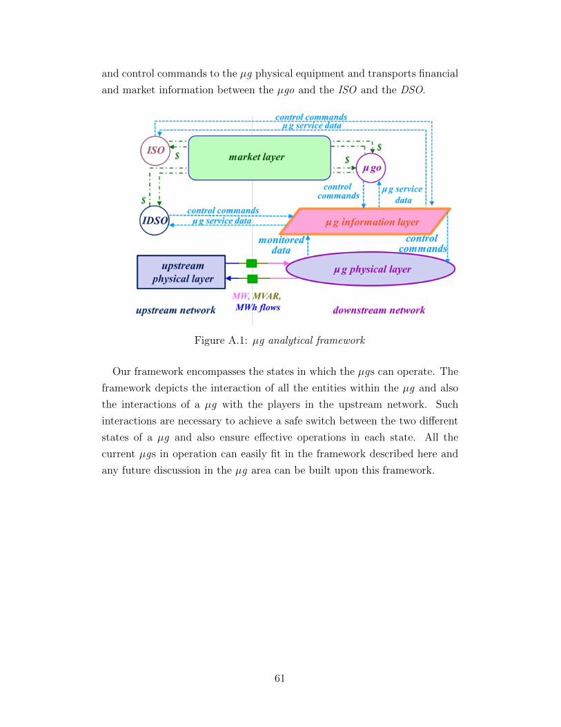
and control commands to the µg physical equipment and transports financial

and market information between the µgo and the ISO and the DSO.

Figure A.1: µg analytical framework

Our framework encompasses the states in which the µgs can operate. The

framework depicts the interaction of all the entities within the µg and also

the interactions of a µg with the players in the upstream network. Such

interactions are necessary to achieve a safe switch between the two different

states of a µg and also ensure effective operations in each state. All the

current µgs in operation can easily fit in the framework described here and

any future discussion in the µg area can be built upon this framework.

61

APPENDIX B

LIST OF SYMBOLS

B.1 General Variables

x[h] the value of any variable x in hour h

(x[h]) m the lower bound on the value of variable x in hour h

(x[h]) M the upper bound on the value of variable x in hour h

H the set of hours defining the scheduling problem period, {h : h =1, ..., H}

x the vector of variable x in hour h, x = [x[1], x[2], ..., x[H]]T

B.2 Steam–Based Variables and Parameters

B the subset of boilers in the CUS, B = {b : b = b1, b2, ..., bB}

B ∨ the subset of low pressure boilers

B ∧ the set of high pressure boilers

s d[h] steam demand or consumed in hour h

η s steam distributing efficiency in the CUS

s b[h] the steam generated by boiler b in hour h

s ρ[h] the steam generated by the HRSG mechanism

s s[h] steam supplied or produced in hour h, s s[h] =∑

b∈B sb[h] + s ρ[h]

62

B.3 Electricity–Based Variables and Parameters

d[h] CUS electricity load demand in hour h

G σ the subset of steam turbine generators

G γ the subset of gas turbine generators

G σ∨the subset of steam turbine generators that work on low pressuresteam

G σ∧the subset of steam turbine generators that work on high pressuresteam

κ ∨ conversion factor of hourly rate of low pressure steam into hourlyrate of electricity generated

κ ∧ conversion factor of hourly rate of high pressure steam into hourlyrate of electricity generated

G the set of generators in the CUS, G = {g : g = σ1, σ2, ..., σS, γ1, γ2, ..., γG}

p G σ∨[h] electricity generated by the steam turbine generators working on

low pressure steam in hour h

p G σ∧[h] electricity generated by the steam turbine generators working on

high pressure steam in hour h

p g[h] electricity generated by the gas turbine generator g ∈ G γ in hourh

p i[h] electricity imported from the wholesale electricity market

p e[h] electricity exported to the wholesale electricity market

B.4 Electricity Grid Variables and Parameters

Notations

N the set of bus indices for the nodes in the CUS electricity network,N = {n : n = 0, 1, ..., N}

L the set of electricity distribution line indices for the CUS electricitydistribution lines, L = {` : ` = 1, ..., L}

63

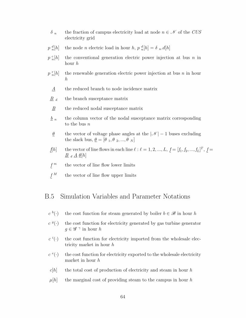
δ n the fraction of campus electricity load at node n ∈ N of the CUSelectricity grid

p dn[h] the node n electric load in hour h, p d

n[h] = δ n.d[h]

p cn[h] the conventional generation electric power injection at bus n in

hour h

p rn[h] the renewable generation electric power injection at bus n in hour

h

A the reduced branch to node incidence matrix

B d the branch susceptance matrix

B the reduced nodal susceptance matrix

b n the column vector of the nodal susceptance matrix correspondingto the bus n

θ the vector of voltage phase angles at the |N | − 1 buses excludingthe slack bus, θ = [θ 1, θ 2, ..., θ N ]

f[h] the vector of line flows in each line ` : ` = 1, 2, ..., L, f = [f1, f2, ..., fL]T , f =B d A θ[h]

f m the vector of line flow lower limits

f M the vector of line flow upper limits

B.5 Simulation Variables and Parameter Notations

c b(·) the cost function for steam generated by boiler b ∈ B in hour h

c g(·) the cost function for electricity generated by gas turbine generatorg ∈ G γ in hour h

c i(·) the cost function for electricity imported from the wholesale elec-tricity market in hour h

c e(·) the cost function for electricity exported to the wholesale electricitymarket in hour h

c[h] the total cost of production of electricity and steam in hour h

µ[h] the marginal cost of providing steam to the campus in hour h

64

λ n[h] the marginal cost of providing electricity at CUS electricity net-work node n in hour h

v[h] the total CO2 emissions in hour h

u[h] the campus unserved energy in hour h

65

REFERENCES

[1] Office of Energy Policy and System Analysis, “Quadrennial energy re-view,” Tech. Rep. April 2015.

[2] North American Electric Reliability Corporation, “Accomodating highlevels of variable generation,” Tech. Rep. April 2009.

[3] D. Bakken, A. Bose, K. M. Chandy, P. P. Khargonekar, A. Kuh, S. Low,A. von Meier, K. Poolla, P. P. Varaiya, and F. Wu, “Grip - grids withintelligent periphery: Control architectures for grid2050,” in Smart GridCommunications (SmartGridComm), 2011 IEEE International Confer-ence on, Oct 2011, pp. 7–12.

[4] R. Arghandeh, M. Brown, A. D. Rosso, G. Ghatikar, E. Stewart, A. Vo-jdani, and A. von Meier, “The local team: Leveraging distributedresources to improve resilience,” IEEE Power and Energy Magazine,vol. 12, no. 5, pp. 76–83, Sept 2014.

[5] Office of Electricity Delivery and Energy Reliability Smart Grid RandDProgram, “DOE microgrid workshop,” Tech. Rep. August 2011.

[6] B. Lasseter, “Microgrids [distributed power generation],” in Power En-gineering Society Winter Meeting, 2001. IEEE, vol. 1, Jan 2001, pp.146–149 vol.1.

[7] G. Venkataramanan and C. Marnay, “A larger role for microgrids,”IEEE Power and Energy Magazine, vol. 6, no. 3, pp. 78–82, May 2008.

[8] S. Bahramirad, A. Khodaei, J. Svachula, and J. R. Aguero, “Buildingresilient integrated grids: One neighborhood at a time,” IEEE Electri-fication Magazine, vol. 3, no. 1, pp. 48–55, March 2015.

[9] New York State Energy Research and Development Authority (NY-SERDA), New York State Department of Public Service (DPS) andNew York State Division of Homeland Security and Emergency Services(DHSES), “Microgrids for critical facility resiliency in new york state,”Tech. Rep. December 2014.

66

[10] G. Gross, “Electricity Resource Planning,” class notes for ECE 588, De-partment of Electrical and Computer Engineering, University of Illinois,Urbana-Champaign Fall 2014.

[11] M. Webster, “The microgrid asset classification real world example:Princeton university,” presented at National Association of RegulatoryUtility Commissioners (NARUC) Winter Committee Meeting 2014.

[12] Chevron Energy Solutions Company for U.S. Department of Energy,“Certs microgrid demonstration with large-scale energy storage and re-newables at santa rita jail,” Tech. Rep. May 2014.

[13] P. M. Costa and M. A. Matos, “Assessing the contribution of microgridsto the reliability of distribution networks,” Electric Power SystemsResearch, vol. 79, no. 2, pp. 382 – 389, 2009. [Online]. Available:http://www.sciencedirect.com/science/article/pii/S0378779608002058

[14] Q. Chen and L. Mili, “Assessing the impacts of microgrids on compositepower system reliability,” in 2013 IEEE Power Energy Society GeneralMeeting, July 2013, pp. 1–5.

[15] A. L. A. Syrri, E. A. M. Cesea, and P. Mancarella, “Contribution of mi-crogrids to distribution network reliability,” in PowerTech, 2015 IEEEEindhoven, June 2015, pp. 1–6.

[16] C. Schwaegerl and L. Tao, “Can microgrids provide a new paradigm fornetwork operation? an evaluation of their technical, commercial, and en-vironmental benefits,” in Electricity Distribution - Part 2, 2009. CIRED2009. The 20th International Conference and Exhibition on, June 2009,pp. 1–18.

[17] N. D. Hatziargyriou, A. G. Anastasiadis, J. Vasiljevska, and A. G.Tsikalakis, “Quantification of economic, environmental and operationalbenefits of microgrids,” in PowerTech, 2009 IEEE Bucharest, June 2009,pp. 1–8.

[18] A. G. Anastasiadis, A. G. Tsikalakis, and N. D. Hatziargyriou, “Op-erational and environmental benefits due to significant penetration ofmicrogrids and topology sensitivity,” in IEEE PES General Meeting,July 2010, pp. 1–8.

[19] Ernest Orlando Lawrence Berkeley National Laboratory, “A frameworkfor the evaluation of cost and benefits of microgrids,” Tech. Rep. Septem-ber 2011.

[20] J. Kleijnen, Statistical Techniques in Simulation - Part 1 and Part 2.New York, USA: Marcel Decker Inc., 1974.

67

[21] University of Illinois at Urbana-Champaign, “Utilities production anddistribution master plan,” Tech. Rep. October 2015.

[22] N. Maisonneuve and G. Gross, “A production simulation tool for systemswith integrated wind energy resources,” IEEE Transactions on PowerSystems, vol. 26, no. 4, pp. 2285–2292, Nov 2011.

[23] Y. Zhang and A. A. Chowdhury, “Reliability assessment of wind inte-gration in operating and planning of generation systems,” in 2009 IEEEPower Energy Society General Meeting, July 2009, pp. 1–7.

[24] J. M. Morales and J. Perez-Ruiz, “Point estimate schemes to solve theprobabilistic power flow,” IEEE Transactions on Power Systems, vol. 22,no. 4, pp. 1594–1601, Nov 2007.

[25] J. M. Morales, A. J. Conejo, and J. Prez-Ruiz, “Simulating the impactof wind production on locational marginal prices,” in Proceedings of the2011 IEEE PES General Meeting, July 2011, pp. 1–1.

[26] Y. Degeilh, “Stochastic simulation of power systems with integrated re-newable and utility-scale storage resources,” PhD thesis, Dept. of Elec-trical Engineering, University of Illinois at Urbana Champaign, 2015,http://gross.ece.illinois.edu/files/2015/03/Yannick-Degeilh.pdf.

[27] R. H. Lasseter and P. Paigi, “Microgrid: a conceptual solution,” inPower Electronics Specialists Conference, 2004. PESC 04. 2004 IEEE35th Annual, vol. 6, June 2004, pp. 4285–4290 Vol.6.

[28] J. D. McDonald, “Microgrids beyond the hype: Utilities need to seea benefit [technology leaders],” IEEE Electrification Magazine, vol. 2,no. 1, pp. 6–11, March 2014.

[29] C. Schwaegerl and L. Tao, The Microgrids Concept in Microgrids: Ar-chitectures and Control. Chichester, UK: John Wiley and Sons Ltd,2013.

[30] C. Marnay, F. J. Robio, and A. S. Siddiqui, “Shape of the microgrid,”in Power Engineering Society Winter Meeting, 2001. IEEE, vol. 1, Jan2001, pp. 150–153 vol.1.

[31] R. H. Lasseter, “Microgrids,” in Power Engineering Society WinterMeeting, 2002. IEEE, vol. 1, 2002, pp. 305–308 vol.1.

68