c 2013 National Technology and Science...
119
Transcript of c 2013 National Technology and Science...


2
c©2013 National Technology and Science Press.
All rights reserved. Neither this book, nor any portion of it, may be copiedor reproduced in any form or by any means without written permission ofthe publisher.

Contents
0 Introduction 5
1 Graphical Convolution 9
2 Step Response of a Second-Order LCCDE 15
3 Car Suspension Analog Model 23
4 Proportional Control System 31
5 Fourier Series Demonstrator 41
6 Image Filter 53
7 Butterworth Filter 61
8 AM Radio Simulator 69
9 Convolution Reverb Audio Effect 79
10 Notch and Comb Filters 85
11 Image Deblurring 93
12 DTMF Decoder 99
A Parts List 109
B TL072 Operational Amplifier 111
C Video Tutorial Links 113

4 CONTENTS
Laboratory Project 0
Introduction
This supplement to Engineering Signals and Systems1 by Ulaby and Yaglecontains twelve hands-on laboratory projects designed to complement mostof the chapters in the textbook. Five of the projects focus on simulationand hardware with NI Multisim and NI ELVIS II, six of the projects re-volve around NI LabVIEW, and one project combines all three tools. Thelab projects are designed to motivate students with engaging and practicalsystems including mechanical system modeling, control systems, image fil-tering and deblurring, AM radio, audio processing, and DTMF decoding.Each lab project guides the students through the activity with detailed in-structions and video-based tutorials to demonstrate specific techniques foreach of the software tools.
This document is fully hyperlinked for section and figure references,and all video links are live hyperlinks. Opening the PDF version of thisdocument is the most efficient way to access all of the links; clicking a videohyperlink automatically launches the video in a browser. Within the PDF,use ALT+leftarrow to navigate back to a starting point.
0.1 Resources
• Appendix A details the parts list required to implement all of the cir-cuits and includes links to component distributors.
• Appendix B describes the Texas Instruments TL072 dual operationalamplifier used in several of the circuits.
1http://www.ntspress.com/publications/engineering-signals-and-systems

6 LABORATORY PROJECT 0. INTRODUCTION
• Appendix C lists all of the available video tutorial links.
0.2 Goals for Student Deliverables
Students should document their work in sufficient detail so that it couldbe replicated by others. Your instructor will provide specific informationregarding the lab report format, e.g., lab notebook, memo, or electronicsubmission. This lab manual uses the symbol “I” to indicate an instruc-tion and “N” to indicate an activity with a reportable result. Numberyour work with the corresponding activity number N to ensure that yourinstructor can quickly locate your work for each numbered activity.
Many of the activities require screen shots of the software tools youused to obtain meaningful information. For NI Multisim and NI ELVISmxscreen shots, circle parameters that you entered or changed away from de-fault values, and highlight regions where you obtained information. Fig-ure 1 illustrates a screenshot from NI Multisim properly highlighted to in-dicate control settings that were adjusted away from default values as wellas regions on the screen where measurements were obtained.
NOTE: Screen shots in Microsoft Word 2010 can be easily captured andhighlighted as follows:
1. Select “Insert” tab and then “Screenshot,”
2. Choose the desired window or select “Screen Clipping” to define anarbitrary region,
3. Select “Shapes,” and
4. Place circles or boxes to highlight important values.

0.2. GOALS FOR STUDENT DELIVERABLES 7
Figure 1: NI Multisim screenshot showing proper markings to indicate con-trol settings adjusted away from default values as well as regions wheremeasurement was obtained.

8 LABORATORY PROJECT 0. INTRODUCTION
0.3 Acknowledgements
I gratefully acknowledge contributions from the following individuals:
• Tom Robbins (NTS Press) for his editorial support throughout thisproject,
• Gretchen Edelmon (National Instruments) for her valuable commentsand feedback regarding the design of the projects,
• Mark Walters (National Instruments) for his helpful support of the NIMultisim product,
• Mark Yoder (Rose-Hulman) for his enthusiastic review of selectedprojects, and
• Rose-Hulman students in Discrete-Time Signals and Systems ECE380(Winter 2012-13) who offered much helpful feedback on their experi-ence with selected projects.
Ed DoeringDepartment of Electrical and Computer EngineeringRose-Hulman Institute of TechnologyTerre Haute, IN 47803

Laboratory Project 1
Graphical Convolution
1.1 Synopsis
Convolution describes the time-domain process by which a linear time-invariant system responds to an input signal. Knowledge of the system’simpulse response permits the system output to be computed for any inputsignal shape.
In this lab project you will determine the impulse response of two first-order systems given their step responses, apply graphical convolution tocalculate the system output for a non-standard signal shape, and then com-pare your calculations to simulation and hardware.
Ulaby/Yagle Sections 2-2 to 2-4
1.2 Objectives
1. Determine the impulse response of a system given its step response
2. Calculate the system output to a non-standard pulse shape
3. Simulate the system output
4. Measure the system output in hardware
5. Compare analytical, simulated, and measured results

10 LABORATORY PROJECT 1. GRAPHICAL CONVOLUTION
1.3 Deliverables
1. Hardcopy of all Multisim circuits and annotated screen shots of sim-ulation results used as the basis of a measurement
2. Hardcopy of all ELVISmx instrumentation screen shots annotated toshow measurement procedures
3. Lab report or notebook formatted according to instructor’s require-ments
1.4 Required Resources
1. NI Multisim
2. NI ELVIS II
3. Resistor: R = 10.0 kΩ
4. Capacitor: C = 0.1 µF
5. Jumper wire kit
1.5 Preparation
Impulse response from step response
Figure 1.1 on the facing page shows two systems implemented as first-order RC circuits. The step response of System A is
ystepA(t) =(
1− e−t/RC)u(t), (1.1)
and the step response of System B is
ystepB (t) = e−t/RCu(t). (1.2)
As discussed in Section 2-2.4 of your text, the impulse response h(t) of thesystem is the time derivative of the step response ystep(t):
h(t) =dystepdt
(1.3)

1.5. PREPARATION 11
Figure 1.1: Two systems implemented as first-order RC circuits: (a) Sys-tem A with grounded capacitor, and (b) System B with grounded resistor.
1 Determine the impulse response waveforms hA(t) and hB(t) for thetwo systems A and B. HINT: hB(t) is the sum of two terms, one of themdue to the step discontinuity at time t = 0. Sketch the impulse responseequations for R = 1 Ω and C = 1 F.
Graphical convolution
Equation 2.30 in your text and replicated below describes how to convolvean input signal x(t) with the system impulse response h(t) to form the out-put y(t):
y(t) = x(t) ∗ h(t) =
∞∫−∞
x(τ)h(t− τ) dτ (1.4)
Graphical convolution provides a visual method to set up the integral forpiecewise-continuous functions.
I Review Section 2-3 in your text, and then follow along with this videotutorial http://youtu.be/zoRJZDiPGds to learn how to apply the graph-ical convolution procedure.
2 Evaluate the impulse response hA(t) for R = 1 Ω and C = 1 F.

12 LABORATORY PROJECT 1. GRAPHICAL CONVOLUTION
3 Apply graphical convolution to determine the output yA(t) of Sys-tem A caused by the system input signal x(t) plotted in Figure 1.2; set theamplitude A to 5 volts.
Figure 1.2: Input signal x(t) with amplitude A.
4 Use a computer plotting tool to visualize yA(t) as a graph over thetime range 0 to 10 seconds.
5 Evaluate yA(t) at the times 2, 4, and 6 seconds.
6 Evaluate the impulse response hB(t) for R = 1 Ω and C = 1 F. Deter-mine yB(t) by recycling as much as possible your results for yA(t). HINT:Your result for hB(t) should include an impulse function δ(t); determinethe system output for this portion of hB(t) and then apply superposition todetermine the complete system output yB(t).
7 Use a computer plotting tool to visualize yB(t) as a graph over thetime range 0 to 10 seconds.
8 Evaluate yB(t) at the times 2, 3.99, 4.01, and 6 seconds.
Video tutorials
Study the following video tutorials that relate to this project:
• NI Multisim:
1.6. SIMULATION 13
– Piecewise linear (PWL) voltage source:http://youtu.be/YYU5WuyebD0
– Plot time-domain circuit response with Transient Analysis:http://youtu.be/waKnad_EXkc
• NI ELVISmx:
– Arbitrary Waveform Generator (ARB):http://decibel.ni.com/content/docs/DOC-12941
– Oscilloscope:http://decibel.ni.com/content/docs/DOC-12942
1.6 Simulation
For this and the subsequent hardware measurements, set R = 10 kΩ andC = 0.1 µF, and change the time scale unit of the plot in Figure 1.2 on thefacing page to milliseconds, i.e., the time span of the signal is 10 ms. Thesevalues permit direct comparison to your analytical results provided thatyou interpret your earlier plots as functions of time in milliseconds.
9 Enter the circuit of System A into NI Multisim. Set up a transientanalysis to plot the circuit input and output over the time span 0 to 10 mswith at least 200 sample points. Use the PIECEWISE_LINEAR_VOLTAGEsource to create x(t).
10 Take cursor measurements of yA(t) at times 2, 4, and 6 ms.
11 Calculate the percent difference between your simulation and yourearlier analytical results from graphical convolution.
12 Repeat these activities for the circuit of System B, taking cursor mea-surements at the times 2, 3.99, 4.01, and 6 seconds.
1.7 Hardware Measurements
I Build System A; use the ELVISmx Arbitrary Waveform Generator tocreate x(t) on the NI ELVIS II analog output A0 with sampling rate set to100 kS/s. Use the ELVISmx Oscilloscope to monitor the input signal x(t)

14 LABORATORY PROJECT 1. GRAPHICAL CONVOLUTION
on the analog input AI6+ and the output signal y(t) on AI7+; remember toground AI6- and AI7-.
I IMPORTANT: Once you are satisfied that the input and output signalslook correct on the oscilloscope, disable the input signal channel and displayonly the output signal to ensure the best possible accuracy.
13 Adjust the oscilloscope settings (especially the trigger settings) tomatch as much as possible your simulation and analysis plots.
14 Take cursor measurements of y(t) at times 2, 4, and 6 ms.
15 Calculate the percent difference between your measurement resultsand your earlier analytical results from graphical convolution.
16 Repeat these activities for System B, taking cursor measurements atthe times 2, 3.99, 4.01, and 6 seconds.
1.8 Discussion
17 Reflect on your analytical, simulation, and hardware measurementresults. How well do these three viewpoints on the same system agreewith each other?
18 How are the systems of System A and System B very similar to eachother?
19 Compare the input and output waveforms for System A. Generallyspeaking what is the effect of System A? Repeat for System B.
Laboratory Project 2
Step Response of a Second-OrderLCCDE
2.1 Synopsis
A second-order linear constant-coefficient differential equation (LCCDE,for short) models a wide range of engineering systems, including mechan-ical, thermal, chemical, and electrical. Understanding the basic propertiesof a second-order LCCDE provides a good foundation for study of manytypes of systems.
In this project you will study the properties of an inductor-capacitor-resistor (LCR) circuit with circuit simulation and then compare your resultsto measurements from the physical circuit.
Ulaby/Yagle Section 2-8
2.2 Objectives
1. Write second-order system parameters in terms of LCR circuit com-ponent values
2. Set up a parameterized transient analysis to plot step response as afunction of resistance
3. Measure damped natural frequency and peak overshoot from under-damped response waveforms
4. Measure rise time

16 LABORATORY PROJECT 2. STEP RESPONSE OF A SECOND-ORDER LCCDE
5. Compare simulation and circuit measurements
2.3 Deliverables
1. Hardcopy of all Multisim circuits and annotated screen shots of sim-ulation results used as the basis of a measurement
2. Hardcopy of all ELVISmx instrumentation screen shots annotated toshow measurement procedures
3. Lab report or notebook formatted according to instructor’s require-ments
2.4 Equipment and Software
1. NI Multisim
2. NI ELVIS II
3. Resistors: R = 1.0 kΩ (4)
4. Capacitor: C = 0.1 µF
5. Inductors: 33 mH (3)
6. Jumper wire kit
2.5 Preparation
Second-order LCCDE
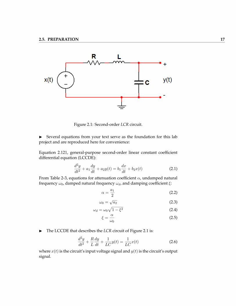
The step response of a second-order linear constant-coefficient differentialequation (abbreviated as “LCCDE”) takes on three distinct forms depend-ing on the damping coefficient ξ; these forms are called underdamped, crit-ically damped, and overdamped. The second-order LCCDE describes awide variety of engineering systems, including the LCR circuit pictured inFigure 2.1 on the next page.
I Study Section 2-8 in your text.
2.5. PREPARATION 17
Figure 2.1: Second-order LCR circuit.
I Several equations from your text serve as the foundation for this labproject and are reproduced here for convenience:
Equation 2.121, general-purpose second-order linear constant coefficientdifferential equation (LCCDE):
d2y
dt2+ a1
dy
dt+ a2y(t) = b1
dx
dt+ b2x(t) (2.1)
From Table 2-3, equations for attenuation coefficient α, undamped naturalfrequency ω0, damped natural frequency ωd, and damping coefficient ξ:
α =a12
(2.2)
ω0 =√a2 (2.3)
ωd = ω0
√1− ξ2 (2.4)
ξ =α
ω0(2.5)
I The LCCDE that describes the LCR circuit of Figure 2.1 is:
d2y
dt2+R
L
dy
dt+
1
LCy(t) =
1
LCx(t) (2.6)
where x(t) is the circuit’s input voltage signal and y(t) is the circuit’s outputsignal.

18 LABORATORY PROJECT 2. STEP RESPONSE OF A SECOND-ORDER LCCDE
1 Write the generic LCCDE coefficients a1, a2, b1, and b2 in terms of thecircuit component values L, C, and R.
2 Write the attenuation coefficient α, the undamped natural frequencyω0, and the damping coefficient ξ in terms of the circuit component values,as well.
3 Calculate α, ω0, and ξ for L = 99 mH,C = 0.1 µF, and four values ofR:500 Ω, 1 kΩ, 2 kΩ, and 4 kΩ. Identify the resistor value (or values) associatedwith underdamped (ξ < 1), critically-damped (ξ = 1), and overdampedstep response (ξ > 1).
4 A “critically-damped” response forms the theoretical boundary be-tween underdamped and overdamped responses. In practice a systemcan be close to this theoretical boundary but will always be either under-damped or overdamped. Identify which of the four resistance values aboveis closest to a critically-damped response.
5 The damped natural frequency ωd serves as a distinct and easily-measuredfeature of the oscillatory nature of an underdamped response, and offers apoint of comparison between theory, simulation, and measurement. Notethat the similarly-named undamped natural frequency ω0 cannot be directlymeasured. Calculate the damped natural frequency ωd for each of the re-sistance values associated with an underdamped response.
Video tutorials
Study the following video tutorials that relate to this project:
• NI Multisim:
– Use a Parameter Sweep analysis to plot resistor power as a func-tion of resistance:http://youtu.be/3k2g9Penuag
– Plot time-domain circuit response with Transient Analysis:http://youtu.be/waKnad_EXkc
– Find the maximum value of a trace in Grapher View:http://youtu.be/MzYK60mfh2Y
• NI ELVISmx:

2.6. CIRCUIT SIMULATION, PART 1 19
– Function Generator (FGEN):http://decibel.ni.com/content/docs/DOC-12940
– Oscilloscope:http://decibel.ni.com/content/docs/DOC-12942
2.6 Circuit Simulation, Part 1
I Enter the circuit of Figure 2.1 on page 17 into NI Multisim. Use aPULSE_VOLTAGE source to create a 1-volt input step signal with zero initialvalue. Set the pulse width to 4 ms and the period to 5 ms.
6 Set up a “Parameter Sweep” analysis based on transient analysis toplot the step response y(t) for each of the four values of R on the samegraph. Set up the transient analysis to run until 2 ms with at least 200 timepoints. Refer to the video tutorial http://youtu.be/waKnad_EXkc re-garding transient analysis setup and http://youtu.be/3k2g9Penuagfor parameter sweep setup; use “List” mode for the “Sweep variation type”and enter a comma-delimited list of the four resistance values. Capture ascreen shot of the plot, and discuss your general observations about thenature of the second-order step as the damping coefficient ξ increases.
7 Take cursor measurements to determine the damped natural frequencyωd. Recall that angular frequency ω is 2π divided by the oscillation periodT . Compare this value by percent difference to the theoretical value youcalculated earlier.
8 Take cursor measurements to determine the peak overshoot of the un-derdamped responses, with peak overshoot defined as the maximum ex-cursion of the signal above its final value.
2.7 Hardware Measurements, Part 1
9 Show how to connect the three available 33 mH inductors to form a99 mH inductor.
10 Show how to connect one or more of the four available 1 kΩ resistorsto create each of the four required resistances 500 Ω, 1 kΩ, 2 kΩ, and 4 kΩ.Hint: Recall what you know about series and parallel equivalent resistance.

20 LABORATORY PROJECT 2. STEP RESPONSE OF A SECOND-ORDER LCCDE
I Build the circuit of Figure 2.1 on page 17:
• Begin with R = 500 Ω.
• Create the circuit input x(t) with NI ELVIS II FGEN and monitor thissignal with AI7+. Connect AI7- to AIGND.
• Connect the circuit output y(t) to AI6+. Connect AI6- to AIGND.
• Set up the ELVISmx Function Generator to drive the circuit input witha 1V step at 200 Hz. Adjust the DC offset so that the input begins at−1 V and reaches 0 V.
• Set up the ELVISmx Oscilloscope to observe the step input x(t) onChannel 0 and the step response y(t) on Channel 1.
I Set the oscilloscope “Timebase” control to 200 µs per division. Adjustthe “Trigger” controls to left-justify the display on the rising edge of theinput x(t). Adjust the “Scale” controls to stretch the traces to fill as muchof the display as possible without clipping. Use the “Run Once” mode andrepeatedly press “Run” until you get an acceptable set of traces.
11 Take cursor measurements to determine the damped natural frequencyωd; refer back to the simulation section for the measurement procedure.Capture a screen shot of the oscilloscope to show your measurement.
12 Record the “Vp-p” (peak-to-peak voltage) value for Channel 1 dis-played below the waveform traces. The oscilloscope reports the differencebetween the observed minimum and maximum values of the trace, there-fore subtract one from this value to obtain the peak overshoot value.
13 Compare (by percent difference) your measured values for ωd andpeak overshoot with those you obtained by simulation. State whether ornot you believe the percent differences to be reasonable.
14 Physical inductors contain a significant effective resistance. Use theELVISmx DMM (digital multimeter) set up as an ohmmeter to measure theresistance of your 99 mH inductor; remember to disconnect the resistorfrom the LCR circuit before you measure resistance.
2.8. CIRCUIT SIMULATION, PART 2 21
2.8 Circuit Simulation, Part 2
I As you have just learned, the physical inductor is not well-modeled bythe ideal inductor in your earlier simulation. To remedy this problem, adda series resistor into the circuit next to the inductor and set its value to theDMM ohmmeter measurement from the previous step.
15 Re-run the parameter sweep to create a new set of step response sig-nals. Capture a screen shot of this updated graph.
16 Take cursor measurements as before to determine the new dampednatural frequency ωd and the peak overshoot. Compare these values bypercent difference to those you obtained from the physical circuit. Discussthe performance of the improved simulation model of the physical circuit.
2.9 Hardware Measurements, Part 2
17 The rise time of the step response is another important descriptor ofthe response waveform. Rise time measures the length of time for the sys-tem to reach 90% of its final steady-state value after the initial step. Takecursor measurements to determine the rise time of each of the four step re-sponse waveforms; set the trigger level to −0.1 V to create a convenient vi-sual marker for the 90% signal crossing. Tabulate your results with columnsfor R, ξ, and rise time. Capture one screen shot for each measurement.

22 LABORATORY PROJECT 2. STEP RESPONSE OF A SECOND-ORDER LCCDE
Laboratory Project 3
Car Suspension Analog Model
3.1 Synopsis
A wide variety of engineering systems – thermal, fluid, mechanical, chemi-cal, electrical – share identical second-order linear constant coefficient differ-ential equation forms. The constants have different dimensions as requiredby the different system types, but the underlying system dynamics such asdamping and oscillation are the same.
In this project you will implement and study an electrical analog to anautomobile suspension system.
Ulaby/Yagle Section 4-3
3.2 Objectives
1. Choose component values for an electrical analog to a mechanicalsystem
2. Determine velocity profile from physical geometry
3. Simulate the system
4. Compare simulation and measurements
5. Use an integrator and differentiator to obtain displacement and accel-eration from velocity

24 LABORATORY PROJECT 3. CAR SUSPENSION ANALOG MODEL
3.3 Deliverables
1. Hardcopy of all Multisim circuits and annotated screen shots of sim-ulation results used as the basis of a measurement
2. Hardcopy of all ELVISmx instrumentation screen shots annotated toshow measurement procedures
3. Lab report or notebook formatted according to instructor’s require-ments
3.4 Equipment and Software
1. NI Multisim
2. NI ELVIS II
3. Resistors: R = 1.0 kΩ (2)
4. Capacitors: C = 0.1 µF (4)
5. Inductors: 33 mH (3)
6. Jumper wire kit
3.5 Preparation
Electrical system analog
A second-order LCR circuit emulates the second-order system dynamics ofthe car suspension. In principle it is possible to choose very large inductorand capacitor values and very small resistor values to exactly match the be-havior of the mechanical system. Unfortunately these extreme values arenot practical. A time scaling technique permits practical component valuesto be selected for the electrical circuit, in effect “shrinking” the car suspen-sion system geometry and operating it on a smaller time scale. For example,the time scale factor S = 1000 means that one second of mechanical systemtime is equivalent to one millisecond of electrical system time. In this sec-tion you will apply the time-scaling technique to derive equations for theLCR circuit values written in terms of the mechanical system coefficients insuch a way that the system dynamics are identical but simply operate on afaster time scale.
3.5. PREPARATION 25
I Study Section 4-3 in your text.
I Several equations from your text serve as the foundation for this labproject and are reproduced here for convenience:
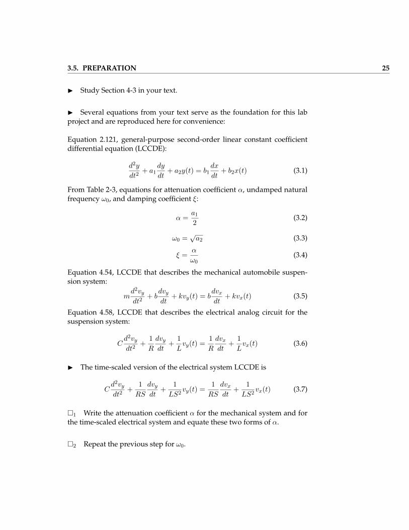
Equation 2.121, general-purpose second-order linear constant coefficientdifferential equation (LCCDE):
d2y
dt2+ a1
dy
dt+ a2y(t) = b1
dx
dt+ b2x(t) (3.1)
From Table 2-3, equations for attenuation coefficient α, undamped naturalfrequency ω0, and damping coefficient ξ:
α =a12
(3.2)
ω0 =√a2 (3.3)
ξ =α
ω0(3.4)
Equation 4.54, LCCDE that describes the mechanical automobile suspen-sion system:
md2vydt2
+ bdvydt
+ kvy(t) = bdvxdt
+ kvx(t) (3.5)
Equation 4.58, LCCDE that describes the electrical analog circuit for thesuspension system:
Cd2vydt2
+1
R
dvydt
+1
Lvy(t) =
1
R
dvxdt
+1
Lvx(t) (3.6)
I The time-scaled version of the electrical system LCCDE is
Cd2vydt2
+1
RS
dvydt
+1
LS2vy(t) =
1
RS
dvxdt
+1
LS2vx(t) (3.7)
1 Write the attenuation coefficient α for the mechanical system and forthe time-scaled electrical system and equate these two forms of α.
2 Repeat the previous step for ω0.
26 LABORATORY PROJECT 3. CAR SUSPENSION ANALOG MODEL
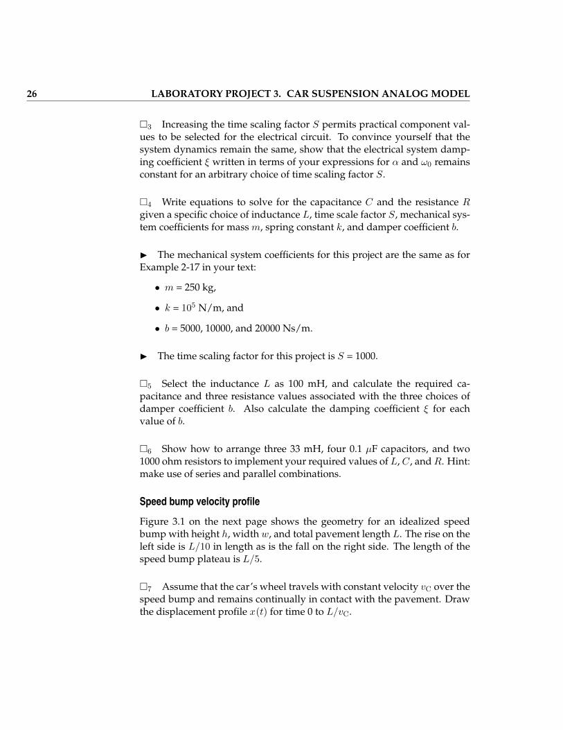
3 Increasing the time scaling factor S permits practical component val-ues to be selected for the electrical circuit. To convince yourself that thesystem dynamics remain the same, show that the electrical system damp-ing coefficient ξ written in terms of your expressions for α and ω0 remainsconstant for an arbitrary choice of time scaling factor S.
4 Write equations to solve for the capacitance C and the resistance Rgiven a specific choice of inductance L, time scale factor S, mechanical sys-tem coefficients for mass m, spring constant k, and damper coefficient b.
I The mechanical system coefficients for this project are the same as forExample 2-17 in your text:
• m = 250 kg,
• k = 105 N/m, and
• b = 5000, 10000, and 20000 Ns/m.
I The time scaling factor for this project is S = 1000.
5 Select the inductance L as 100 mH, and calculate the required ca-pacitance and three resistance values associated with the three choices ofdamper coefficient b. Also calculate the damping coefficient ξ for eachvalue of b.
6 Show how to arrange three 33 mH, four 0.1 µF capacitors, and two1000 ohm resistors to implement your required values of L, C, andR. Hint:make use of series and parallel combinations.
Speed bump velocity profile
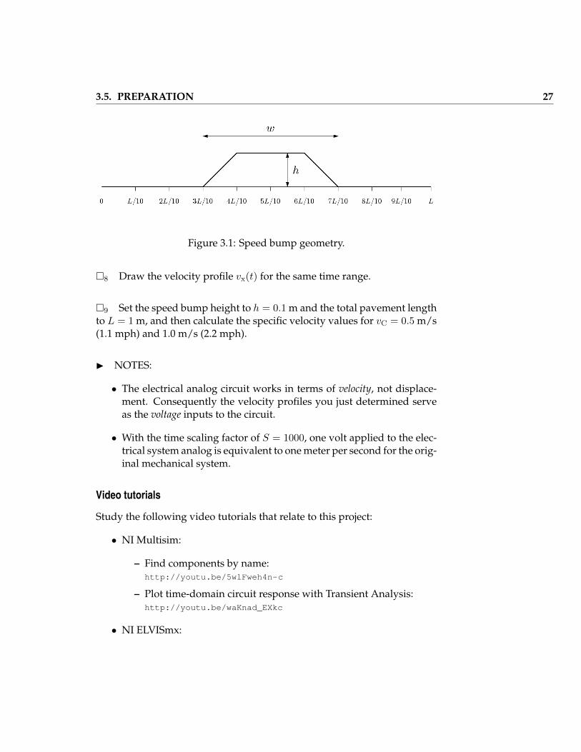
Figure 3.1 on the next page shows the geometry for an idealized speedbump with height h, width w, and total pavement length L. The rise on theleft side is L/10 in length as is the fall on the right side. The length of thespeed bump plateau is L/5.
7 Assume that the car’s wheel travels with constant velocity vC over thespeed bump and remains continually in contact with the pavement. Drawthe displacement profile x(t) for time 0 to L/vC.
3.5. PREPARATION 27
Figure 3.1: Speed bump geometry.
8 Draw the velocity profile vx(t) for the same time range.
9 Set the speed bump height to h = 0.1 m and the total pavement lengthto L = 1 m, and then calculate the specific velocity values for vC = 0.5 m/s(1.1 mph) and 1.0 m/s (2.2 mph).
I NOTES:
• The electrical analog circuit works in terms of velocity, not displace-ment. Consequently the velocity profiles you just determined serveas the voltage inputs to the circuit.
• With the time scaling factor of S = 1000, one volt applied to the elec-trical system analog is equivalent to one meter per second for the orig-inal mechanical system.
Video tutorials
Study the following video tutorials that relate to this project:
• NI Multisim:
– Find components by name:http://youtu.be/5wlFweh4n-c
– Plot time-domain circuit response with Transient Analysis:http://youtu.be/waKnad_EXkc
• NI ELVISmx:
28 LABORATORY PROJECT 3. CAR SUSPENSION ANALOG MODEL
– Arbitrary Waveform Generator (ARB):http://decibel.ni.com/content/docs/DOC-12941
– Oscilloscope:http://decibel.ni.com/content/docs/DOC-12942
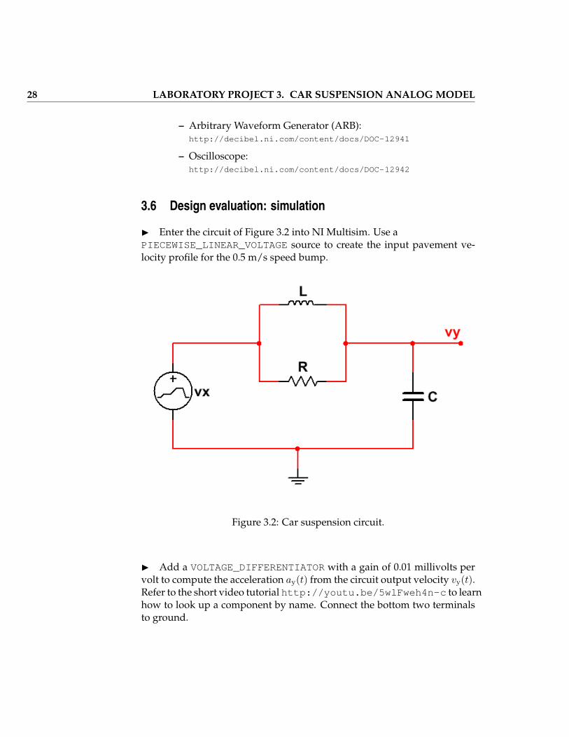
3.6 Design evaluation: simulation
I Enter the circuit of Figure 3.2 into NI Multisim. Use aPIECEWISE_LINEAR_VOLTAGE source to create the input pavement ve-locity profile for the 0.5 m/s speed bump.
Figure 3.2: Car suspension circuit.
I Add a VOLTAGE_DIFFERENTIATOR with a gain of 0.01 millivolts pervolt to compute the acceleration ay(t) from the circuit output velocity vy(t).Refer to the short video tutorial http://youtu.be/5wlFweh4n-c to learnhow to look up a component by name. Connect the bottom two terminalsto ground.
3.7. DESIGN EVALUATION: HARDWARE 29
I Add a VOLTAGE_INTEGRATOR with a gain of 5000 volts per volt tocompute the displacement y(t) from the circuit output velocity vy(t). Con-nect the bottom two terminals to ground.
I Set up a transient analysis to run until 2 ms with at least 500 time points.
10 Plot four variables: the input velocity vx(t) and the three outputs (dis-placement, velocity, and acceleration). Capture a screen shot of all fourvariables for each of the three values of R, taking care to use the samevertical-axis scale for each plot to facilitate easy comparison. Label thescreen shot with the value of R and ξ.
11 Discuss your findings, noting the effects of damping coefficient ξ onthe behavior of each of the three output quantities.
12 Create a second version of the piecewise-linear voltage source for the1.0 m/s speed bump, and then capture another set of screen shots for eachof the three values of R. Remember to label the screen shots as in the pre-vious step.
13 Discuss your findings, noting the effects of damping coefficient ξ onthe behavior of each of the three output quantities. Also comment on theeffect of increased vehicle speed over the speed bump.
3.7 Design evaluation: hardware
I Build the circuit of Figure 3.2 on the preceding page:
• Set up the ELVISmx Arbitrary Waveform Generator to create the 0.5 m/sspeed bump velocity profile vx(t) on the NI ELVIS II analog output A0with sampling rate set to 200 kS/s.
• Use the ELVISmx Oscilloscope to monitor the input velocity profilevx(t) on the analog input AI6+ and the output velocity profile vy(t)on AI7+; remember to ground AI6- and AI7-.
I Set the oscilloscope “Timebase” control to 200 µs per division. Adjustthe “Trigger” controls to place the velocity profile in the center of the dis-play.
30 LABORATORY PROJECT 3. CAR SUSPENSION ANALOG MODEL
14 Capture a screen shot for each of the three values of R, labeling themwith the values of R and ξ as before.
I Create the 1.0 m/s speed bump velocity for the arbitrary waveformgenerator. Use the same total length.
15 Apply the new speed bump velocity profile to your circuit and cap-ture another set of screen shots for the three values of R.
3.8 Discussion
16 Evaluate the agreement between your physical circuit measurementsand the simulation results. Identify one or two numerical measurementssuch as peak value or oscillation frequency and report the percentage dif-ference between the two.
17 Recall that force is proportional to acceleration, i.e., the familiar equa-tion F = ma. Study your plots for the acceleration profile ay(t). Recogniz-ing that a seat-belted passenger experiences the same force as the car mass,discuss how your results for acceleration relate to the forces exerted on thepassengers as the car passes over the speed bump for various automobilespeeds and damping coefficients.
18 Explain why experimenting with the electrical analog to the mechan-ical system provides an advantage compared to experimenting with themechanical system itself.
Laboratory Project 4
Proportional Control System
4.1 Synopsis
Control systems improve the performance of a physical mechanism by us-ing negative feedback. In this lab project you will study a simple proportionalcontrol system that speeds up the responsiveness of an emulated DC motor.
Ulaby/Yagle Section 4-8
4.2 Objectives
1. Analyze a proportional control system to determine open-loop andclosed-loop performance in terms of time constant and steady-stateerror
2. Design a proportional control system to achieve specified performanceimprovements
3. Implement the control system with op-amp modules
4. Evaluate the design with simulation
5. Implement and evaluate the design in hardware
6. Compare design calculations, simulation results, and measurementresults
7. Study the qualitative performance of the proportional control system

32 LABORATORY PROJECT 4. PROPORTIONAL CONTROL SYSTEM
4.3 Deliverables
1. Hardcopy of all Multisim circuits and annotated screen shots of sim-ulation results used as the basis of a measurement
2. Hardcopy of all ELVISmx instrumentation screen shots annotated toshow measurement procedures
3. Lab report or notebook formatted according to instructor’s require-ments
4.4 Equipment and Software
1. NI Multisim
2. NI ELVIS II
3. TI TL072 dual op-amp (2 devices)
4. Resistors: R = 1.0 kΩ, R = 47 kΩ (2), R = 100 kΩ (2); four additionalresistors to be calculated
5. Capacitor: C = 4.7 µF, electrolytic
6. Jumper wire kit
4.5 Preparation
Proportional controller analysis
Figure 4.1 on the facing page shows the block diagram of a proportionalcontrol system that contains the following elements and signals:
• Mechanism, M(s): The physical mechanism that performs useful workbut whose properties such as reaction time to a change in its inputmay be too slow. In this lab project the mechanism is an RC circuitthat simulates the behavior of a DC motor.
• Summing junction: Compares the control input x(t) to the controlledoutput y(t) to produce the error signal e(t) = x(t) − y(t). The controlinput expresses the desired motor speed, and the error signal indi-cates how well the actual motor speed matches the desired speed.

4.5. PREPARATION 33
Figure 4.1: Proportional control system.
• Proportional gain, KP: This block amplifies the error signal to pro-duce the control effort signal c(t).
• Actuator gain, KA: This block further amplifies the control effort toproduce the actuator effort applied to the motor input.
• Plant, H(s): The cascade combination of the two gain stages and themechanism.
• Feedback, G(s): The feedback path is taken as unity in this project.
Figure 4.2 shows the circuit emulator of the DC motor mechanism.
Figure 4.2: DC motor emulated by an RC circuit.
1 Derive the open-loop transfer function of the mechanism M(s) = Vout(s)/Vin(s).NOTE: Write this and all subsequent transfer functions in the standardform of a unity coefficient on the highest power of s in the denominator.
34 LABORATORY PROJECT 4. PROPORTIONAL CONTROL SYSTEM
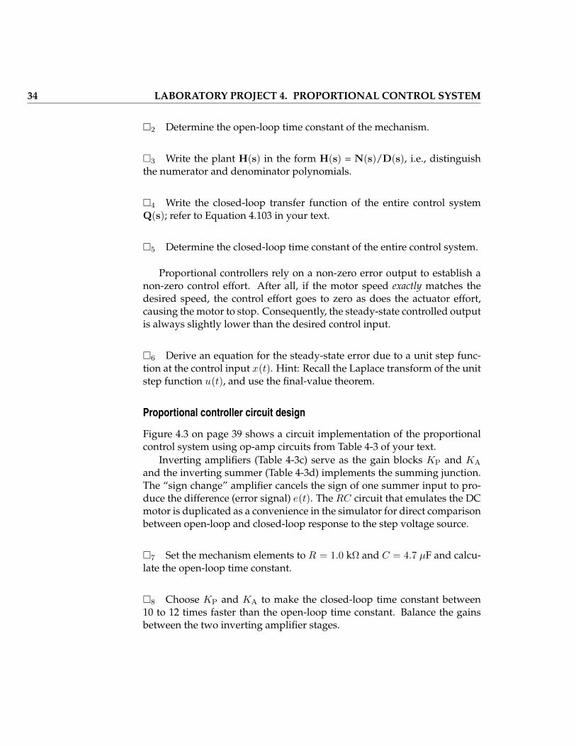
2 Determine the open-loop time constant of the mechanism.
3 Write the plant H(s) in the form H(s) = N(s)/D(s), i.e., distinguishthe numerator and denominator polynomials.
4 Write the closed-loop transfer function of the entire control systemQ(s); refer to Equation 4.103 in your text.
5 Determine the closed-loop time constant of the entire control system.
Proportional controllers rely on a non-zero error output to establish anon-zero control effort. After all, if the motor speed exactly matches thedesired speed, the control effort goes to zero as does the actuator effort,causing the motor to stop. Consequently, the steady-state controlled outputis always slightly lower than the desired control input.
6 Derive an equation for the steady-state error due to a unit step func-tion at the control input x(t). Hint: Recall the Laplace transform of the unitstep function u(t), and use the final-value theorem.
Proportional controller circuit design
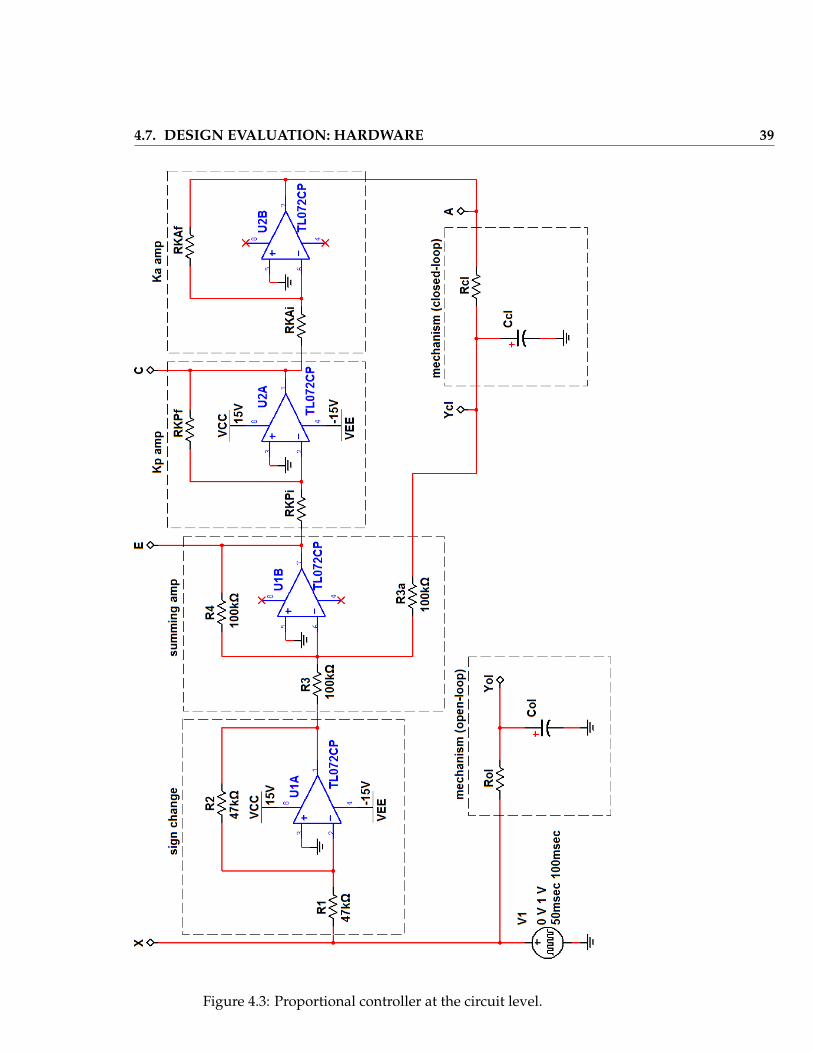
Figure 4.3 on page 39 shows a circuit implementation of the proportionalcontrol system using op-amp circuits from Table 4-3 of your text.
Inverting amplifiers (Table 4-3c) serve as the gain blocks KP and KA
and the inverting summer (Table 4-3d) implements the summing junction.The “sign change” amplifier cancels the sign of one summer input to pro-duce the difference (error signal) e(t). The RC circuit that emulates the DCmotor is duplicated as a convenience in the simulator for direct comparisonbetween open-loop and closed-loop response to the step voltage source.
7 Set the mechanism elements to R = 1.0 kΩ and C = 4.7 µF and calcu-late the open-loop time constant.
8 Choose KP and KA to make the closed-loop time constant between10 to 12 times faster than the open-loop time constant. Balance the gainsbetween the two inverting amplifier stages.

4.6. DESIGN EVALUATION: SIMULATION 35
9 Choose resistor values RKPf , RKPi, RKAf , and RKAi to implement thegains you calculated in the previous step. Keep all resistor values in the 1Kto 100K range.
10 Based on your four resistor values, calculate the closed-loop time con-stant and the steady-state error expressed as a percentage.
Video tutorials
Study the following video tutorials that relate to this project:
• NI Multisim:
– Find components by name:http://youtu.be/5wlFweh4n-c
– Place dual op amp second device:http://youtu.be/-QDFEf-KdEw
– Plot time-domain circuit response with Transient Analysis:http://youtu.be/waKnad_EXkc
– Set cursor to a specific value:http://youtu.be/48sQja58I10
• NI ELVISmx:
– Function Generator (FGEN):http://decibel.ni.com/content/docs/DOC-12940
– Oscilloscope:http://decibel.ni.com/content/docs/DOC-12942
4.6 Design evaluation: simulation
I Enter the circuit of Figure 4.3 on page 39 into NI Multisim. Use theTL072CP dual op-amp model and the PULSE_VOLTAGE source to apply aunit step control input. Place “on-page connectors” to name the signal netsof interest.
I Set up a transient analysis to run until 10 ms with at least 200 timepoints. Select the labeled signal nets X, Yol, and Ycl for display.
36 LABORATORY PROJECT 4. PROPORTIONAL CONTROL SYSTEM
11 Take cursor measurements to determine the open-loop and closed-loop time constants as well as the closed-loop steady-state error. Measurethe time constant as the time it takes for the output to reach 63% of its finalvalue after the step is applied.
12 Report the percentage difference between your simulation results andyour design results. Comment on the level of agreement between these twosets of results. Refine your design as necessary to comply with the designspecifications of a 10 to 12 times speedup of the time constant.
13 Modify the transient analysis to add plots of the error signal E, negatedcontrol effort C (add an expression “-C” to cancel the effect of the invertingamplifier sign), and the actuator effort A.
14 Study the plots of the various internal controller signals and discusshow the proportional controller is able to achieve its speedup of the DCmotor.
4.7 Design evaluation: hardware
I Build the circuit of Figure 4.3 on page 39:
• Use only oneRC circuit for the DC motor emulator to permit a propercomparison of open-loop vs. closed-loop performance. Remember toobserve the polarity of the electrolytic capacitor.
• Use the TI TL072C dual op-amp or equivalent device; refer to Ap-pendix B on page 111 for details. Power the op-amps with the NIELVIS II ±15-volt dual supply.
• Create the control input x(t) with NI ELVIS II FGEN and monitor thissignal with AI7+. Connect AI7- to AIGND.
• Set up the ELVISmx Function Generator to drive the input with a 1Vstep at 10Hz. Adjust the DC offset so that the input begins at 0V andreaches 1V.
• Set up the ELVISmx Oscilloscope to observe the control input x(t) onChannel 0.
• Set up the ELVISmx Oscilloscope to observe other signals within thecontroller by displaying AI6+ on Channel 1. Connect AI6- to AIGND.

4.7. DESIGN EVALUATION: HARDWARE 37
I Temporarily disconnect the input of the DC motor emulator from thecontroller and drive it directly from the function generator. Adjust the os-cilloscope timebase and vertical scale to fill the screen as much as possiblewith signals x(t) and yOL(t).
15 Measure the open-loop time constant using the same cursor tech-nique that you used with the simulator.
16 Reconnect the DC motor emulator to the rest of the controller. Mea-sure the closed-loop time constant and steady-state error.
17 Report the percentage difference between your measured and sim-ulated results for time constants and steady-state error. Comment on thelevel of agreement.
I If necessary, trouble-shoot your design by observing intermediate sig-nals within the controller and comparing those to your simulator results.
Qualitative behavior of the controller
I Set up the oscilloscope for a consistent horizontal and vertical scale forall subsequent measurements:
• Timebase = 10ms/div,
• Vertical Scale = 200mV/div (both channels),
• Vertical position = 0 (both channels),
• Trigger type = edge, slope = rising, source = Channel 0, and level =0.5
I Maintain the same function generator amplitude and frequency usedearlier.
18 As you did earlier, temporarily connect the DC motor emulator inopen-loop mode. Display the open-loop output for square, sine, and tri-angle waveforms. Discuss the ability of the open-loop system to accuratelytrack the desired input waveform, and specifically comment on what workswell and what does not.
38 LABORATORY PROJECT 4. PROPORTIONAL CONTROL SYSTEM
19 Reconnect the DC motor emulator for closed-loop operation. Displaythe closed-loop output for the same three waveform shapes, and then dis-cuss the ability of the closed-loop system to accurately track the desiredinput waveform. Specifically comment on what works well and what doesnot; also compare the performance of the closed-loop system to the open-loop system, and state the improvements that you observe.
20 Display the actuator effort for the same three waveform shapes. Dis-cuss how the actuator effort relates to the controller input waveform, i.e.,how must the actuator operate to improve the performance of the DC mo-tor responsiveness?
4.7. DESIGN EVALUATION: HARDWARE 39
Figure 4.3: Proportional controller at the circuit level.

40 LABORATORY PROJECT 4. PROPORTIONAL CONTROL SYSTEM
Laboratory Project 5
Fourier Series Demonstrator
5.1 Synopsis
Any periodic signal x(t) has a Fourier series representation in which suit-ably scaled and phase shifted sinusoids of increasing frequency sum to-gether to form x(t). Adding together a finite number of sinusoids createsan approximation to x(t).
In this project you will create a Fourier series demonstrator in LabVIEW.The interactive demonstrator will allow you to experience a variety of ef-fects due to a finite number of sinusoids as well as the effects of phase dis-tortion and the consequence of ignoring phase entirely. Your applicationwill also create a waveform data file for the ELVISmx Arbitrary WaveformGenerator and get you started learning how to use the ELVISmx DynamicSignal Analyzer to measure amplitude spectra.
Ulaby/Yagle Section 5-4
5.2 Objectives
1. Implement an interactive Fourier series demonstrator application inLabVIEW
2. Study signals resulting from a truncated Fourier series
3. Study Gibbs phenomenon
4. Study the effects of phase distortion and complete absence of phaseinformation

42 LABORATORY PROJECT 5. FOURIER SERIES DEMONSTRATOR
5. Use the ELVISmx Dynamic Signal Analyzer (DSA) to measure ampli-tude spectra
5.3 Deliverables
1. Hardcopy of all LabVIEW block diagrams and front panels that youcreate
2. Screen shots of requested spectrum/time plots
3. Lab report or notebook formatted according to instructor’s require-ments
5.4 Required Resources
1. NI ELVIS II
2. NI LabVIEW with MathScript RT Module
5.5 Preparation
Fourier series mathematics
I Study Section 5-4 in your text.
1 Study the Fourier series descriptions of Waveforms 1, 2, 4, 6, 7, and8 in Table 5-4 of your text; this list will henceforth be called the “selectedwaveforms.” For each of these waveforms identify the expressions for an,bn, and a0, the dc (average) value of the waveform.
2 State how to write the amplitude and phase form of the Fourier series,i.e., how to write cn and φn in terms of the sine/cosine coefficients an andbn.
Fourier series demonstrator construction tips
Figure 5.1 on page 50 shows the front panel of the Fourier series demon-strator LabVIEW application you will create in this project. The application

5.5. PREPARATION 43
constructs selected waveforms from Table 5-4 by adding N terms of the in-finite series. The application interactively displays the waveform xt(t) andits associated amplitude/phase spectrum as the N slider control varies.
I Read through these construction tips for the front panel and then referback to this step as needed while you construct the application; each tiprefers to the letter indicator on Figure 5.1 on page 50:
A Menu control with enumerated data type; see video tutorial http://youtu.be/tImN4C03W1k
B File Path Control: Right-click on the folder icon, choose “Browse Op-tions,” and choose “New or existing.”
C Button control: Right-click on the button, choose “Mechanical Action,”and select “Switch Until Released.”
D Stop button: Right-click on the button, select “Properties,” select the“Key Navigation” tab, and set “Toggle” to “Escape.” This way youcan stop the application by pressing the “ESC” key.
E Plot legend: Right-click on the waveform graph, select “Visible Items,”uncheck “Plot Legend,” and check “Graph Palette.”
F Horizontal Pointer Slide: Right-click, select “Visible Items,” and check“Digital Display.” Again right-click, select “Representation,” and choose“I32” to setN as an integer. Double-click the upper limit of the slider’snumerical scale to change the value to 200.
G Plot style: After you place the waveform graph indicator, click the centerof the plot legend, select “Common Plots,” and choose the discretelines icon in the center of the lower row. Afterwards hide the plotlegend.
H Numerical indicator display precision: After you create the array indi-cator, select an individual numerical display, right-click and choose“Display Format,” and then select “Floating point,” 4 digits, and set“Precision Type” to “Digits of precision.”
I Save front panel control default values by choosing “Edit” then “MakeCurrent Values Default” to save effort when you close and re-open the VI.

44 LABORATORY PROJECT 5. FOURIER SERIES DEMONSTRATOR
I Turn off auto-scaling on the y-axis of the waveform graph indicators tomaintain a fair comparison between one waveform to another.
Figure 5.2 on page 51 shows the block diagram of the Fourier seriesdemonstrator LabVIEW application you will create in this project. A Math-Script node contains all of the Fourier series calculations. The event-structureand while-loop combination executes the MathScript node only when avalue changes on a front panel control; refer to the tutorial video http://youtu.be/eGlvOiqYVxg for more details on event structures. Theblock diagram also includes a feature to write the text file representationof x(t) that can be loaded directly into the ELVISmx Arbitrary WaveformGenerator.
I Read through these construction tips for the block diagram and thenrefer back to this step as needed while you construct the application; eachtip refers to the letter indicator on Figure 5.2 on page 51:
A Execute the event structure one time when the application first runs; seethe tutorial video http://youtu.be/UFEvmmggqLQ for details.
B Make the event structure respond to all front panel controls; do not deletethe “Timeout” event.
C MathScript tips:
• Access MathScript help and also experiment with syntax by us-ing the interactive MathScript Window available on the “Tools”menu.
• Right-click on the MathScript node frame and choose “Add In-put” and “Add Output” to create connection terminals. Notethat a variable must already exist in the MathScript text before“Add Output” will display any variables.
• Set up the time axis as an array: t=0:dt:P*T0-dt where “dT”is the waveform period T0 divided by the number of samplesper period NS and “P” is the number of periods to display.
• Set up “n” as an array n=1:N.
• Create a new array y initialized to zero values and of the samelength as an existing array x by writing y=x-x, i.e., subtract theexisting array from itself.
• Use the element-by-element (array style) math operations .*(multiplication), ./ (division), and .^ (exponentiation).

5.5. PREPARATION 45
• Use the switch construct to choose which of the selected wave-forms to create; type help switch in the MathScript Windowfor details; the tutorial video http://youtu.be/tImN4C03W1kalso shows how to set up a switch statement. Create the a0, an,and bn coefficients by directly translating the Fourier series coef-ficient equations of Table 5-4 in your text. MathScript providesthe constant π as pi.
• Waveforms 2 and 4 require zero coefficients for n even. Multiplythe coefficient expression by |sin(nπ/2))| to zero out the evencoefficients. For example, the coefficient calculation for Wave-form 2 is bn=((4*A)./(n*pi)).*abs(sin(n*pi/2)).
• Form the amplitude coefficients ascn=real(sqrt(an.^2 + bn.^2)); the “real()” function en-sures that the MathScript node does not automatically create acomplex-valued array.
• Form the phase coefficients aspn = -atan2(bn,an)*(1-pd).*(cn>1e-10). The function“atan2()” properly returns an angle in any of the four quadrants;“atan()” can only return an angle in quadrants 1 and 4. The “pd”(phase distortion) value allows a variable amount of phase dis-tortion to be introduced. Multiplying by the inequality test setsall phase values to zero for sufficiently small amplitude coeffi-cients.
• Form the displayed amplitude coefficient array as cndisp = [a0 cn]to ensure that the front panel waveform graph indicator x-axisscale appears correctly. Note that MathScript arrays are 1-indexedmeaning that the first array element is index 1. This differs fromLabVIEW arrays that are 0-indexed.
• Form the displayed phase coefficient array in a similar way ascndisp, using zero as the first element. Convert the phase fromradians to degrees by multiplying by 180/pi.
• Use a for loop to implement the sum for x(t); type help for inthe MathScript Window for details. Remember to initialize thewaveform array x to the same length as the time array t beforeyou start the loop.
D “Write to Spreadsheet File” built-in subVI: Right-click on the “delim-iter” terminal and choose “Create Constant.” Right-click on the newly-
46 LABORATORY PROJECT 5. FOURIER SERIES DEMONSTRATOR
created constant, enable ’\’ Codes Display and enter \n (new-line) as the delimiter character.
E Bundle the waveform array into a waveform data type to ensure that thex-axis scale appears correctly for x(t).
5.6 Fourier Series Demonstrator Implementation
In this section you will create the Fourier series demonstrator LabVIEWapplication VI.
I Create the front panel and block diagram as pictured in Figures 5.1 onpage 50 and 5.2 on page 51.
I Enter the MathScript code to calculate the Fourier series coefficient andwaveform arrays for the selected waveforms from Table 5-4 from your text.You may wish to debug your code using the interactive MathScript Win-dow.
I Test each of the front panel controls to ensure that your demonstratorapplication work correctly. You should find that all of the selected wave-forms look like sinusoids at N = 1 and then progressively become moredistinct as you increase the front panel slide control for N .
5.7 Fourier Series Study
Experiment with your Fourier series demonstrator application to gain ex-perience with the following concepts. Set the front panel control values tomatch those pictured in Figure 5.1 on page 50.
Gibbs phenomenon
Gibbs phenomenon is the characteristic “ringing” or oscillation that ap-pears at waveform discontinuities.
3 Which of the selected waveform numbers shows Gibbs phenomenon?Collect screen shots of these waveforms and state the value of N for eachwaveform.

5.8. ELVISMX DYNAMIC SIGNAL ANALYZER 47
4 What is distinctive about the waveforms that do not show Gibbs phe-nomenon?
Minimum number of components
Study the minimum number of frequency components necessary to makea recognizable waveform.
5 For each of the selected waveforms determine the minimum numberof frequency components required to make the waveform appear visuallyindistinguishable from the ideal waveform pictured in Table 5-4 of yourtext.
Phase distortion
The sum of sinusoidal components technique to create an arbitrary periodicwaveform involves an amplitude spectrum as well as a phase spectrum.Explore the effect of phase distortion up to complete absence of phase in-formation.
6 For each of the selected waveforms investigate phase distortion valuesfrom 0 (no phase distortion) up to 1 (complete distortion, all phase compo-nents set to zero). Collect representative screen shots to show the impact ofvarying degrees of phase distortion on the waveform.
5.8 ELVISmx Dynamic Signal Analyzer
The ELVISmx Dynamic Signal Analyzer (DSA) provides a real-time spec-trum display of a signal applied to the analog NI ELVIS II input.
I Start the DSA and study its panel controls.The “FFT Settings” control the Fast Fourier Transform computation that
serves as the heart of the DSA. These critical settings must be carefully se-lected to obtain correct amplitude spectrum measurements of periodic sig-nals. First learn how the DSA takes a measurement and then experimentwith the settings in a moment.
The DSA repetitively captures a snapshot of the input signal with du-ration “Resolution (lines)” (R) divided by “Frequency Span” (fspan); thistime-domain record appears below the frequency display.
48 LABORATORY PROJECT 5. FOURIER SERIES DEMONSTRATOR
When measuring a periodic signal the captured time-domain signalmust contain an integer multiple of periods, consequently R/fspan dividedby the signal period T0 must be an integer N and the frequency span maybe readily calculated as
fspan =R
NT0, (5.1)
where fspan is the frequency span in Hz, R is the resolution in “lines” (sam-ple points), T0 is the period of the periodic input signal in seconds, and Nis the number of periods captured. N = 10 cycles provides a good startingpoint for most measurements.
I Set up your Fourier series demonstrator front panel controls to matchthose pictured in Figure 5.1 on page 50.
I Save this waveform to a text file (click the “Save” button on your frontpanel).
I Start the ELVISmx Arbitrary Waveform Generator (ARB) and open thewaveform editor. You should see a default segment of 10 ms length. Select“File” and open the text file you created; you should see the same wave-form you saw in your demonstrator application. Set the sample rate to200 kHz. Select “File” again, choose “Save As,” and select the “WaveformFile (.wdt)” option.
I Return to the ARB main panel and open the .wdt file you just created;be sure to enable the channel output. Set the update rate to “200k” andstart the generator.
I Use the ELVISmx Oscilloscope to ensure that you are in fact producinga signal on the analog output you selected in the previous step. Stop theoscilloscope when you are finished.
I Return to the ELVISmx Dynamic Signal Analyzer (DSA). Set the reso-lution to R = 400 lines.
7 Calculate the required span frequency fspan to capture exactly 10 pe-riods of your waveform. Remember to account for the fact that the ARBproduces two cycles in 10 ms.
5.8. ELVISMX DYNAMIC SIGNAL ANALYZER 49
I Use the default DSA settings except for the following:
• Frequency Display:
1. Units = Linear
2. Mode = Peak
• Cursor Settings:
1. Cursors On = enabled
2. Cursor Select = C1
8 Capture a screen shot of the DSA display.
9 Measure the amplitude spectrum for odd values of n from 1 to 5 usingCursor 1; take the square root of the displayed cursor value “dVpk^2” toobtain the voltage amplitude. IMPORTANT: Position Cursor 2 between apair of spectral lines to set its measured value to zero; the value displayedas dVpk^2 is the difference between the two cursors and you want Cursor 2to serve as the zero reference. Tabulate your measurements and compareusing percent difference to the amplitude coefficients calculated by yourFourier series demonstrator application. Additional helpful tips:
• Use the cursor position buttons to make fine adjustments in the vicin-ity of a spectral line; these are the pair of gray diamonds at the bottomcenter of the DSA.
• Double-click the upper limit value on the horizontal frequency axisand select a lower value to zoom in on the lower-frequency spectrallines. Do not change the “Frequency Span” value for this purposebecause this changes the measurement itself.
10 Discuss the level of agreement you found between the theoretical am-plitude spectrum values and those measured by the DSA.
11 Change the frequency display units to “dB” and collect a screen shotof this result. Discuss the relative advantages and disadvantages of thisdisplay mode compared to the linear display mode.

50 LABORATORY PROJECT 5. FOURIER SERIES DEMONSTRATOR
Figure 5.1: Front panel of the Fourier series demonstrator application.

5.8. ELVISMX DYNAMIC SIGNAL ANALYZER 51
Figure 5.2: Block diagram of the Fourier series demonstrator application.

52 LABORATORY PROJECT 5. FOURIER SERIES DEMONSTRATOR

Laboratory Project 6
Image Filter
6.1 Synopsis
The Fourier transform provides a convenient way to filter signals, and eas-ily extends to multiple dimensions such as two-dimensional image signals.
In this project you will build a 2-D image filter based on the Fast FourierTransform (FFT), and then study the effect of filter parameters such as cut-off frequency and filter order on the processed image.
Ulaby/Yagle Sections 5-8 and 5-13
6.2 Objectives
1. Use the 2-D Fast Fourier Transform (FFT) to convert from the spatialdomain to the frequency domain
2. Devise a 2-D Butterworth image filter from a 1-D magnitude response
3. View image spectra with dynamic range compression
4. Implement a complete image filter in MathScript
5. Study the effects of cutoff frequency, filter order, and center frequencyfor low-pass, band-pass, high-pass, and band-stop image filters
6.3 Deliverables
1. Hardcopy of all MathScript code that you create
54 LABORATORY PROJECT 6. IMAGE FILTER
2. Screen shots of requested spectrum/time plots
3. Lab report or notebook formatted according to instructor’s require-ments
6.4 Required Resources
1. NI LabVIEW with MathScript RT Module
2. Images supplied by your instructor (NOTE: 256×256 pixel 8-bit graylevel images work best for this project)
6.5 Preparation
Frequency-domain filtering
I Review Sections 5-8 and 5-13 in your text.
I Study the tutorial video http://youtu.be/X53SrMnu91A to learnhow the Fourier transform implements two-dimensional image filtering asthe product of a frequency-domain image and a two-dimensional filter.
I The one-dimensional Butterworth filter serves as the basis for the fourfilter styles you will implement in this project (low pass, high pass, bandpass, and band stop); study the tutorial video http://youtu.be/QJdNVdL4iBQto learn more.
I A one-dimensional filter easily converts to a two-dimensional filter bychanging the frequency variable ω to the radial distance r from zero fre-quency (DC) in the frequency-domain u-v plane. Study the tutorial videohttp://youtu.be/qpwUHt-DEbs to learn how.
Image processing with MathScript
The LabVIEW MathScript Window and scripting environment will be usedfor this project.
I Study the tutorial video http://youtu.be/Tvi1oY0lV2g to learnbasic operations with the MathScript Window.

6.5. PREPARATION 55
I Learn everything you need to work with images in MathScript withthis tutorial video http://youtu.be/oM_KSYIDrE4.
I Type help followed by each of these commands and functions thatwill contribute to your image filter MathScript code; study the help page toensure that you understand each one:
• File path and directory
– pwd
– cd
– dir
• Image files and image display
– figure
– title
– close; look for the close all option
– fread_image
– view_image
– size
• FFT
– fft2d
– fftshift
– ifft2d
• Miscellaneous functions and statements
– meshgrid
– real
– sqrt
– log10
– abs
– if

56 LABORATORY PROJECT 6. IMAGE FILTER
6.6 Image Filter Implementation
In this section you will gradually create the complete image filter Math-Script code.
I Open the MathScript Window and create a new script file.
I Start your script with clear and close all to clear the variables andclose all figure windows.
I Remember to thoroughly document your code with liberal use of ‘%’comment lines.
I Use cd to set the current directory to the folder where you have storedthe image files.
1 Use fread_image to load an image file into the variable f; rememberto end the line with a semicolon to suppress echoing of the image data tothe MathScript output window. Type whos at the command line or selectthe “Variables” tab to determine the dimensions of the image. Report thename of the image you used and its dimensions; confirm that the image issquare, i.e., that it has the same number of pixels in both dimensions.
2 Use view_image to display the image, and then use title to labelthe image. Collect a screen shot of the figure display window.
I Set the variable N to the image size using the size function. Be sureto call size with appropriate options to return a single scalar value ratherthan an array of values; you may assume that the images you use are al-ways square.
I Convert the image to its frequency-domain form F using fft2d; re-member that MathScript is case sensitive, therefore f and F are distinctvariable names.
6.6. IMAGE FILTER IMPLEMENTATION 57
3 Report the data type of F (use whos at the command line or look atthe “Variables” tab). Also report the maximum absolute value of F us-ing max(max(abs(F))); compare this value to the maximum value of theoriginal image f.
4 Ceate a new figure window using figure and then view the imagespectrum magnitude abs(F) with view_image. Collect a screen shot ofthe image and comment on its appearance.
5 As you discovered a moment ago the maximum absolute value of theimage spectrum is very large compared to that of the image itself. The im-age spectrum has a much higher dynamic range than the image, and becauseview_image automatically scales the gray level display according to themaximum value most of the interesting features disappear. To remedy thisproblem, it is common to display the logarithm spectrum (similar to deci-bels) as log10(1 + |F |). Capture a screen shot of the log image spectrumand comment on its appearance. IMPORTANT NOTE: The log operationis simply for display purposes; be sure to use F for subsequent filteringcalculations.
6 Carefully study your original image spectrum and log image spec-trum images. Do you notice anything special about the upper left cornerof the image? This is the location of DC (zero frequency). Use fftshiftto shift the DC location to the center of the image. Note that you can embedfunctions in other functions, therefore you can write F=fftshift(fft2d(f))to take care of the shifting operation as part of the FFT calculation. Capturea screen shot of the shifted log image spectrum and then draw the u-v planeaxes directly on the image. Try to interpret what you see by realizing thatthe center of the u-v plane is DC, low frequencies are close to the center,and increasingly-high frequencies occur as you move farther away fromDC; compare the image spectrum to the original spatial-domain image.
I Create the u-v plane index images with [u,v]=meshgrid2d(-N/2:(N-1)/2).You may find it instructive to look at the numerical values of these two ar-rays for a small value of N, say 8. Each value of the u array corresponds tothe u coordinate in the u-v plane, and similarly each value of v correspondsto the v coordinate. Any given index into the u and v arrays, say, u(1) andv(1), provides the u and v coordinates for that index.

58 LABORATORY PROJECT 6. IMAGE FILTER
I Create the r (radius) plane as r =√u2 + v2. Remember to use array-
style exponentiation, i.e., .^2; without the period, MathScript interpretsu^2 as a matrix product. As in the previous step, look at the result of thisstep for N=8. You should find that zero appears in the center of the arrayand that values become increasingly large away from the center.
I Create the 2-D Butterworth lowpass filter Mlp based on the equationpresented in http://youtu.be/qpwUHt-DEbs using r − rcenter as thefrequency variable. The constant offset rcenter allows the filter passband tobe moved away from DC to a new center frequency, thereby converting thelowpass filter into a bandpass filter. Remember to use array-style divisionand exponentiation.
I Place the Butterworth filter parameters near the beginning of your scriptfor convenience.
I Create the 2-D highpass filter Mhp based on your result from the low-pass filter. Use an if statement to select between the lowpass and highpassfilters to create the filter M. View the 2-D Butterworth filter as an image inits own figure window.
I Apply the filter M to the image spectrum F to create the filtered spec-trum G (again, remember array-style math operations). Display the filteredlog magnitude spectrum its own figure window.
I Transform the filtered image spectrum G back to the spatial-domainimage g with the inverse FFT ifft2d – remember to apply fftshiftbefore you take the inverse FFT to restore the DC location to the upper leftcorner.
7 Check the data type of g; you should see that the image is complex-valued. Study the array values for g in the “Variable” tab, and then reportthe typical value of the imaginary component. Explain why either real orabs could be used to convert the result of the inverse FFT to a real-valuedimage. Display the filtered image in its own figure window.

6.7. IMAGE FILTERING STUDY 59
I As you are by now aware, the newly-created figure windows overlapexisting windows. You can easily cause each figure window to appear in apredefined position:
• Define the display height and width of your monitor with variablesh and w.
• Enter the line set(gcf,’Position’,[0 h/2 w/3 h/2]) imme-diately after the first view_image line in your script. This commandplaces the current figure (gcf means “get current figure”) with itslower left corner on the far left of the display and halfway up (theseare the first two values of the four-element array), sets the figure’shorizontal dimension to one third of the display width, and sets itsvertical dimension to one half of the display height.
• Place a similar command after each view_image to tile your displaywith all five figure windows.
I Test your finished script with several values each of cutoff frequencyrc, filter order n, and center frequency rcenter for the lowpass and for thehighpass filters. Ensure that your script produces expected results.
I Go back and insert comments as necessary to finalize the documenta-tion on your script. Include your name and other identifying informationrequired by your instructor.
6.7 Image Filtering Study
Experiment with your image filter application to better understand the ef-fect of each of the filter parameters: cutoff frequency rc, filter order n, andcenter frequency rcenter.
Lowpass and bandpass filters
8 Set rcenter = 0 and n = 3 for the lowpass filter. Experiment with thecutoff frequency rc to determine values that make the filtered image appearextremely blurred, moderately blurred, and only slightly blurred. Capturea screen shot of the entire tiled image display for each case and report rcfor each image. Discuss your results.
60 LABORATORY PROJECT 6. IMAGE FILTER
9 Set rcenter = 0 and Set rc = 20. Experiment with the filter order n. Cap-ture a screen shot of the entire tiled image display for n = 1, 5, and 50.Discuss the overall effect of n on the Butterworth filter image, the filteredspectrum, and the output image.
10 Set rc = 10 and n = 3. Experiment with the center frequency rcenterto center the passband near low frequencies, mid frequencies, and high fre-quencies. Capture a screen shot of each and report rcenter for each image.Discuss the overall effect of rcenter on the Butterworth filter image, the fil-tered spectrum, and the output image.
Highpass and bandstop filter
11 Repeat Activity 8 with the high-pass filter selected.
12 Repeat Activity 10 with the high-pass filter selected.

Laboratory Project 7
Butterworth Filter
7.1 Synopsis
In this project you will design an active Butterworth lowpass filter to meetspecified target values for DC gain and cutoff frequency. Once you haveconfirmed that your filter design meets specifications you will investigatethe filter’s ability to suppress high-frequency noise superimposed on a digital-like information signal.
Ulaby/Yagle Section 6-8
7.2 Objectives
1. Design a filter transfer function
2. Design and evaluate an active filter
3. Compare simulated and measured frequency response
4. Evaluate a filter’s ability to remove high-frequency noise
7.3 Deliverables
1. Hardcopy of all Multisim circuits and annotated screen shots of sim-ulation results used as the basis of a measurement
2. Hardcopy of all ELVISmx instrumentation screen shots annotated toshow measurement procedures
62 LABORATORY PROJECT 7. BUTTERWORTH FILTER
3. Lab report or notebook formatted according to instructor’s require-ments
7.4 Equipment and Software
1. NI Multisim
2. NI ELVIS II
3. TI TL072 dual op-amp
4. Resistors: two (values to be calculated)
5. Capacitors: two to three (values to be calculated)
6. Jumper wire kit
7.5 Preparation
Butterworth filter design
I Study Section 6-8 in your textbook.
1 Design a second-order Butterworth lowpass filter transfer function toobtain the following target values:
• DC gain = 1 (0 dB) and
• Cutoff frequency fc = 800 Hz.
Recall that angular frequency is ωc = 2πfc.
2 Figure 7.1 on the facing page shows the circuit schematic of the Sallen-Key active filter circuit and the transfer function implemented by the cir-cuit. Match the coefficients of your Butterworth filter transfer function tothe Sallen-Key transfer function. Derive equations to calculate the two ca-pacitor values C1 and C2 for the special case of R1 = R2 = R.

7.6. DESIGN EVALUATION: SIMULATION 63
Figure 7.1: Sallen-Key active filter circuit with associated transfer function.
3 Use your equations to select four readily-available component valuesfrom the parts list of Appendix A on page 109 to construct the Sallen-Keycircuit. Keep the resistor values between 1 kΩ and 100 kΩ. Report the per-cent difference between your selected values and the exact values requiredby your design equations. You may combine two standard-valued compo-nents to obtain a needed value, e.g., two parallel capacitors each with valueC to yield an effective capacitance 2C.
7.6 Design evaluation: simulation
I Enter the circuit of Figure 7.1 into NI Multisim. Use the resistor andcapacitor values that you will eventually use to build the circuit. Use the

64 LABORATORY PROJECT 7. BUTTERWORTH FILTER
TL072CP dual op-amp model and the AC_VOLTAGE source to apply a si-nusoidal input. Place “on-page connectors” to name the signal nets Vi andVo.
4 Set up an AC analysis to create a Bode-style frequency response plotof Vo/Vi over the range 10 Hz to 10 kHz. Use dB (decibels) scale for thevertical axis.
5 Take cursor measurements to determine the DC gain and the cutofffrequency fc; remember that the gain at the cutoff frequency is 3 dB downfrom the gain at DC. Report the percentage difference between your simu-lation results and the target design values; comment on the level of agree-ment between these two sets of results.
I Iterate on your design (recalculate component values and resimulate)until the DC gain is within 1 dB of the target DC gain and the cutoff fre-quency is within 10% of the target fc.
Video tutorials
Study the following video tutorials that relate to this project:
• NI Multisim:
– Find components by name:http://youtu.be/5wlFweh4n-c
– AC (sinusoidal) voltage source:http://youtu.be/CXbuz7MVLSs
– VCC and VEE power supply voltages:http://youtu.be/XkZTwKD-WjE
– Display and change net names:http://youtu.be/0iZ-ph9pJjE
– Measure frequency response with AC Analysis:http://youtu.be/tgCPDBtRcso
– Plot mathematical expression:http://youtu.be/qYVf_rkTF-o
– Set cursor to a specific value:http://youtu.be/48sQja58I10

7.7. DESIGN EVALUATION: HARDWARE 65
• NI ELVISmx:
– Function Generator (FGEN):http://decibel.ni.com/content/docs/DOC-12940
– Arbitrary Waveform Generator (ARB):http://decibel.ni.com/content/docs/DOC-12941
– Oscilloscope:http://decibel.ni.com/content/docs/DOC-12942
– Bode Analyzer:http://decibel.ni.com/content/docs/DOC-12943
7.7 Design evaluation: hardware
I Build the circuit of Figure 7.1 on page 63:
• Use the TI TL072C dual op-amp or equivalent device; refer to Ap-pendix B on page 111 for details. Power the op-amp with the NIELVIS II ±15-volt dual supply.
• Create the signal input Vin with NI ELVIS II FGEN and monitor thissignal with AI6+. Connect AI6- to AIGND.
• Set up the ELVISmx Function Generator to drive the filter input witha 1V amplitude sinusoid.
• Set up the ELVISmx Oscilloscope to observe the filter input Vi onChannel 0 and Vo on Channel 1 with connections to AI7+. ConnectAI7- to AIGND.
I Observe the filter input and output while you vary the frequency of thefunction generator over a large range. Confirm that the circuit behaves likea lowpass filter with unity gain in the passband and substantial attenuationin the stopband.
6 Set up the ELVISmx Bode Analyzer to plot the frequency response ofthe filter:
• Stimulus Channel: AI6
• Response Channel: AI7

66 LABORATORY PROJECT 7. BUTTERWORTH FILTER
• Start Frequency: 10 Hz
• Stop Frequency: 9.0 kHz
• Steps: 20 per decade
• Peak Amplitude: 1.00
• Mapping: Logarithmic
7 Set up the Bode Analyzer to sweep in a small frequency range from700 to 900 Hz; increase the step size as needed to obtain a good measure-ment of the −3 dB frequency. Compare this measurement to your simu-lated value for fc as well as the design target value.
7.8 Filter high-frequency noise
In this section you will create a digital-like information signal (squarewave)that has been corrupted with high-frequency sinusoidal noise and investi-gate how the lowpass filter passes the information signal while suppressingthe noise.
8 Perform a single-frequency AC simulation in Multisim to determinethe filter’s gain at 200 Hz and also at 5 kHz.
9 Predict the filter’s output amplitude for a 1-volt amplitude 200 Hzsinusoid applied to the filter input. Repeat for a 4-volt amplitude 5 kHzsinusoid.
I Set up the ELVISmx Arbitrary Waveform Generator to create the sumof a 1-volt amplitude 200 Hz squarewave (the information signal) and a4-volt amplitude 5 kHz sinusoid (the interfering noise signal) on analogoutput AO0, and apply this signal to the filter input. Use the maximumavailable sampling frequency of 200 kS/s and a 5 ms segment length.
10 Observe the filter input and output for the signal-plus-noise wave-form. Take screen shots of the input waveform and the output waveformindividually.

7.8. FILTER HIGH-FREQUENCY NOISE 67
11 Discuss how well the Butterworth filter removes the high-frequencynoise.

68 LABORATORY PROJECT 7. BUTTERWORTH FILTER

Laboratory Project 8
AM Radio Simulator
8.1 Synopsis
In this lab project you will create an AM radio simulator that features anaudio signal viewer to simultaneously display the frequency spectrum andtime-domain representations of any desired signal in the system and playthe signal on the sound card. The specific baseband and carrier frequenciesspecified in this project make it possible for you to listen to the spectrumyou see, thereby enhancing your intuitive insights about the AM modula-tion and demodulation process.
Ulaby/Yagle Section 6-11
8.2 Objectives
1. Develop an intuitive understanding of the modulation and demodu-lation process
2. Build an AM radio simulator in LabVIEW
8.3 Deliverables
1. Hardcopy of all LabVIEW block diagrams and front panels that youcreate
2. Screen shots of requested spectrum/time plots

70 LABORATORY PROJECT 8. AM RADIO SIMULATOR
3. Lab report or notebook formatted according to instructor’s require-ments
8.4 Required Resources
1. NI LabVIEW
8.5 Preparation
AM radio theory
I Study Section 6-11 in your text.
I Figure 8.1 on the next page shows the block diagram of the LabVIEWAM radio simulator that you will construct in this lab project. Comparethe section labeled “Three AM transmitters” to Figures 6-58 and 6-64(b) inyour text; this section of the LabVIEW VI models three AM transmittersoperating at three distinct carrier frequencies. Also compare the sectionlabeled “AM receiver” to Figure 6-63 in your text. The LabVIEW VI directlyimplements the block diagram of the superheterodyne receiver pictured inyour text.
8.6 AM Transmitters
I Create an empty top-level VI to serve as the starting point of your AMradio simulator application.
Global variables
I Global variables reduce block diagram wiring clutter, an especially use-ful technique for this project because most subVIs require the same valuesuch as system sampling frequency. Study the video http://youtu.be/PquslTj69f4 to learn how to create a global variable, how to place it in aVI, how to change the variable from write mode to read mode, and how toextend the number of elements contained in the global variable.

8.6. AM TRANSMITTERS 71
Figure 8.1: Top-level VI block diagram of the AM radio simulator.
I Create the global variable VI global.vi that contains four controls oftype DBL:
• f_s [Hz] – system sampling frequency in Hz; default value = 22050
• dur [s] – signal duration in seconds; default value = 0.1
• f_max [Hz] – maximum frequency in Hz of the baseband signalsources, also called signal bandwidth; default value = 500
• f_IF [Hz] – intermediate frequency in Hz used by the AM receiver;default value = 750
72 LABORATORY PROJECT 8. AM RADIO SIMULATOR
I Place four global variables on your radio simulator VI as in the “SystemConstants” area of Figure 8.1 on the preceding page. Create constants todocument the values of the global variables.
Baseband signal sources
I Follow along with the video http://youtu.be/C2zYeC_RpM8 tocreate a sinusoidal signal generator subVI sine.vi that accepts the de-sired oscillation frequency f0 [Hz] as an input and produces the signalas an array output.
I Follow along with the video http://youtu.be/R3h4_uR9Dcc tocreate an audio signal viewer subVI viewer.vi that accepts a signal ar-ray as input and produces two graph outputs, one to show the frequencyspectrum of the signal and the other to show the time-domain signal. Alsoinclude the Play Waveform Express subVI to listen to the signal on thesoundcard.
IMPORTANT: Protect your hearing! Before running this VIwhen wearing ear buds or headphones, first turn the volumeall the way down, and then gradually increase the volume to acomfortable level. In later steps this VI produces high-frequencysounds that could damage your hearing if you have the volumetoo high.
I Place and connect sine.vi and viewer.vi in your radio simulatorVI. Create waveform graph indicators on the front panel to display thespectrum and time-domain signals. Try several values of oscillation fre-quency, and confirm that the displays look correct, and also confirm thatyou can hear the signal on your soundcard.
I Copy your sinusoidal signal generator subVI file to a new file triangle.vi;edit this subVI to create a triangle-wave signal based on the built-in TriangleWave subVI found in the same subpalette as Sine Wave.
I Copy your sinusoidal signal generator subVI file to a new file dual_sine.vi;edit this subVI to create a dual-sine tone: the first tone frequency is f0 withunit amplitude and the second tone frequency is 1.7 times f0 amplitude 0.7.
8.6. AM TRANSMITTERS 73
1 Create screen captures of your radio simulator VI front panel for eachof your three baseband signal sources, each set to 500 Hz. Adjust the up-per limit of the time-domain time axis so that you can clearly see severalperiods of the waveform.
I Adjust the three baseband signal frequencies to match those shown onthe block diagram of Figure 8.1 on page 71.
AM modulator
I Create the subVI AM_mod.vi that modulates its baseband input signalarray according the AM modulation equation ym(t) = [A+x(t)] cos(2πfct).Create an input f_c [Hz] to serve as the carrier frequency. Select the con-stant A as |xmin(t)|, i.e., the absolute value of the most negative value of theinput signal array; see the built-in subVI Array Max & Min. This choiceof A corresponds to a modulation index of 1; refer to Section 6-11.5 in yourtext for a discussion of modulation index.
2 Update your radio simulator VI to place an AM modulator subVI be-tween the sinusoidal signal generator and the signal viewer. Try severaldifferent carrier frequencies and signal frequencies. Discuss in some de-tail your observations about the effect of AM modulation on the basebandsignal.
I Add two more AM modulators, one after each of your two remainingsignal sources. Use carrier frequencies 2500, 3750, and 5000 Hz. Add thethree modulated signal together (Compound Arithmetic works nicelyhere), and then connect to your signal viewer.
3 Create a screen capture of your radio simulator VI front panel. NOTE:At this point your VI models the effect of several AM broadcasters operat-ing in a given locality. Comment on the apparent requirements to keep thetransmitters from “stepping” on each other’s signals.

74 LABORATORY PROJECT 8. AM RADIO SIMULATOR
8.7 AM Receiver
RF filter
I Follow along with this video http://youtu.be/gBVluWy_UGs tocreate a bandpass filter subVI BPF.vi that processes an input signal arrayto produce an output array. The subVI includes an input to set the desiredcenter frequency fc as well as a Boolean control input to disable the filter,i.e., to pass the input to the output with no processing. Use a 10th-orderButterworth filter from the Signal Processing subpalette with the highcutoff frequency set to fc+fmax and the low cutoff frequency set to fc−fmax.
I Update your radio simulator VI to place a bandpass filter as the firststage of the AM receiver.
Local oscillator and mixer
I Continue updating your radio simulator VI by placing sine.vi toserve as the local oscillator, and then a multiplier to serve as the mixer.
I Place a front panel control to serve as the “tuning knob” of the AMreceiver; the round knob or horizontal pointer slide works nicely for thispurpose. The tuning knob selects the center frequency of the first-stagebandpass filter, thereby choosing the carrier frequency of the desired AMbroadcaster. The local oscillator frequency fLO tracks the carrier frequencyas fLO = fc−fIF. Note that this is a different choice than that suggestedby Equation 6.128 in your text because the intermediate frequency is lowerthan the lowest broadcaster frequency to emulate the commercial AM radiostandard (fIF=455 kHz for fc between 530 and 1610 kHz).
I Now is an appropriate time to enclose your design in an event structureto make your VI interactive. Follow along with the video http://youtu.be/eGlvOiqYVxg to learn how to place the event structure, adjust it torespond to changes in the tuning knob control, and exit when the “stop”button is pressed.
NOTE: The event structure does not trigger when you first runthe VI, giving the impression that nothing happened as a re-sult of modifying the block diagram. Nudge the tuning knob’sdigital display value up and then back down to see the result
8.7. AM RECEIVER 75
of a modification without changing the tuning knob’s value;right-click the tuning knob and select “Visible Items” to enablethe digital display. For a more sophisticated approach, studythe video tutorial http://youtu.be/UFEvmmggqLQ to learnhow to execute the event structure one time when you first runthe VI.
4 Connect your signal viewer to the mixer output. Create a Booleanconstant for the bandpass filter enable; set the constant to “false” so thatthe filter is disabled. Experiment with different values of the tuning knobranging from 750 Hz and up to 5 kHz; double-click each limit of your front-panel knob and enter these limits. Discuss how the spectrum changes inresponse to different values of the local oscillator frequency. In particular,comment on how the spectrum of a desired station can be translated to theintermediate frequency.
5 Now enable the bandpass filter and continue your experimentationwith the tuning knob. Discuss the primary benefit of the bandpass filter asregards translation of the desired station to the intermediate frequency.
I Adjust the limits on your tuning knob to select among only the carrierfrequencies pictured on the diagram of Figure 8.1 on page 71.
IF filter
6 Place a second bandpass filter after the mixer output; this is the IF fil-ter, consequently set the filter center frequency to fIF. Connect your signalviewer to the IF filter output and experiment with the tuning knob again.Discuss the primary benefit of the IF filter as regards translation of the de-sired station to the intermediate frequency.
Demodulator
I Review Figure 6-60 in your text; this envelope detector circuit serves asthe AM demodulator and can be implemented by an absolute value opera-tor followed by a lowpass filter.

76 LABORATORY PROJECT 8. AM RADIO SIMULATOR
I Copy your bandpass filter subVI file to a new file LPF.vi; edit thissubVI to create a lowpass filter; change the filter type to “Lowpass” and setthe low cutoff frequency set to fmax. Disconnect the high cutoff frequencywire, and then delete the front panel control for fc.
7 Update your radio simulator VI with the absolute value node and low-pass filter. Connect your signal viewer to the lowpass filter output. Createa Boolean constant for the lowpass filter enable; set the constant to “false”so that the filter is disabled. Experiment with the tuning knob to select eachof the three stations. Discuss how the spectrum changes in response to dif-ferent values of the local oscillator frequency. Specifically comment on howthe absolute value operator modifies the spectrum.
8 Now enable the lowpass filter and repeat your experimentation withthe tuning knob. Discuss the role of the lowpass filter.
DC blocker
The audio amplifier is the final stage of the superheterodyne receiver of Fig-ure 6-63 in your text. While amplification is not critical for this simulation,the DC blocking feature of the audio amplifier is worth simulating.
I Create the subVI DC_blocker.vi to remove the DC component (av-erage value) of the demodulator output. See the built-in subVI AC & DCEstimator in the signal processing subpaletter that calculates the average(DC) value of an array.
I Place DC_blocker as the final stage of your radio simulator VI. Con-nect the signal viewer and ensure that the DC value is indeed removedfrom the signal.
8.8 Discussion
I Set the tuning knob to select the triangle-wave baseband signal. Adjustthe vertical axis of the spectrum display to the range 0 to 1 (turn off autoscaling, too), adjust the vertical axis of the time-domain display to the range−1 to 1 (turn off auto scaling), and adjust the horizontal axis of the time-domain display to the range 0 to 0.05; in this way you have a common axisscaling for all plots to be collected.

8.8. DISCUSSION 77
9 Collect a screen shot of your radio simulator front panel at each la-beled signal point in Figure 8.1 on page 71, i.e., 1c, 2c, and 3 to 9.
10 Discuss how will the final AM receiver output matches the originalbaseband signal.
11 Discuss your new understanding of AM radio. Specifically commenton any new insights that you gained.

78 LABORATORY PROJECT 8. AM RADIO SIMULATOR

Laboratory Project 9
Convolution Reverb Audio Effect
9.1 Synopsis
Discrete convolution serves as the foundation of a popular audio process-ing technique called convolution reverberation or “convolution reverb” forshort. Convolution reverb uses the impulse response (IR) recorded withina physical room or hall to artificially add reverberation to an audio signalsuch as an instrument or voice.
In this lab project you will gain familiarity with the LabVIEW built-insubVI Convolution as a means to convolve small sequences, and then applythis subVI to implement your own convolution reverb audio effect.
Ulaby/Yagle Section 7-5
9.2 Objectives
1. Evaluate the discrete-time convolution sum by hand
2. Confirm by-hand calculations with the LabVIEW Convolution subVI
3. Implement a convolution reverb effect using speech and recorded im-pulse response (IR) audio files
9.3 Deliverables
1. Hardcopy of all LabVIEW block diagrams and front panels that youcreate

80 LABORATORY PROJECT 9. CONVOLUTION REVERB AUDIO EFFECT
2. .zip file containing all audio files that you create
3. Lab report or notebook formatted according to instructor’s require-ments
9.4 Required Resources
1. NI LabVIEW with MathScript RT Module
2. Speech .wav file from the Open Speech Repository, http://www.voiptroubleshooter.com/open_speech
3. Impulse response .wav file from Open Air, http://www.openairlib.net
4. Resample Audio .wav VI http://decibel.ni.com/content/docs/DOC-23105
9.5 Preparation
By-hand computation of discrete-time convolution
As an initial warm-up on the subject of discrete-time convolution, viewthis short video tutorial http://youtu.be/yyTu0SXeW1M to learn howto convolve two sequences by hand. Apply what you have learned by con-volving the following pairs of sequences:
1 1, 2, 3 ∗ 3, 2, 1
2 0, 0, 1, 1, 1, 1, 1 ∗ 0.2, 0.2, 0.2, 0.2, 0.2
3 0, 0, 1, 1, 1, 1, 1 ∗ −1, 1
4 1, 2, 3 ∗ 1, 0, 0, 0, 0, 0, 0.75, 0, 0, 0, 0, 0, 0.33, 0, 0, 0, 0, 0, 0.1
Confirm by-hand computation
I Follow along with this video tutorial http://youtu.be/Fsf88Rmimz4to learn how to create a LabVIEW VI to evaluate the convolution of two se-quences, and to visualize the input and output sequences as arrays and asstem plots.
9.6. CONVOLUTION REVERB AUDIO EFFECT 81
5 Run your VI for each of the sequence pairs above. TIP: Delete an el-ement from the array by right-clicking on the element and choosing “DataOperations | Delete Element.” Collect a screen shot of the front panel foreach sequence pair, and then compare to your by-hand calculations. Recon-cile any differences between the two by correcting your by-hand calculationor by revising your LabVIEW code.
Download and prepare audio files
I Visit the Open Speech Repository, http://www.voiptroubleshooter.com/open_speech. Follow the link for your language of choice, and thendownload one or more of the speech audio clips.
I Visit Open Air, http://www.openairlib.net. Follow the “IR Data”tab at the top of the page and investigate the available rooms and halls. Af-ter you select a specific location, click the “Impulse Responses” tab. Seek animpulse response (IR) audio file that is mono, i.e., single channel. Down-load one or more of the available IR audio files.
I Download the LabVIEW VI Resample Audio .wav available at http://decibel.ni.com/content/docs/DOC-23105. Use this applicationto produce a set of speech and IR audio files that have the same samplingfrequency. Choose a standard sampling frequency such as 44.1 kHz.
9.6 Convolution reverb audio effect
Reverberation is a mass of echoes that cannot be individually perceivedas discrete echos. Begin your design by creating a simple IR that containsdistinct echoes for testing purposes.
I Study the video tutorial http://youtu.be/ChSVf9lZ44k to learnhow to read and write .wav audio files, how to extract the audio file as a1-D array for processing, and how to listen to the audio within the VI.
6 Create a LabVIEW VI that generates an IR .wav file containing fourunit values (impulses) separated by silence (zero values) at intervals 50,500, and 900 ms. That is, the signal array looks like a 1 at n = 0 followedby 50 ms of silence, and then another 1, and then 500 ms of silence, and so
82 LABORATORY PROJECT 9. CONVOLUTION REVERB AUDIO EFFECT
on. Remember to calculate the number of zeros in the silent regions usingthe same sampling frequency that you used for your speech and IR files.MathScript or a combination of Initialize Array and Replace Array Subsetworks well for this part. NOTE: Type Ctrl+Space to search for LabVIEWsubVIs by name.
7 Create a LabVIEW VI to read your speech and IR .wav files, convolvethem, and then write the processed audio to a file.
• Remove the Convolution “algorithm” constant to revert back to thedefault method “frequency domain.”
• IMPORTANT: Place the Quickscale subVI in the “Signal Processing| Signal Operations” subpalette just after the convolution subVI toensure the audio signal does not exceed the ±1 signal limits whichwould result in audible clipping noise.
• Add waveform graphs to plot the speech, IR, and processed audioarrays.
• Include three instances of the Play Waveform Express subVI to listento each audio signal; connect the output error cluster of the first subVIto the input error cluster of the next subVI to guarantee the correctorder of audio playback as speech, the IR, and then the processedaudio.
8 Test your convolution audio effect with the speech audio and the four-echo IR you created earlier. Discuss your test results. Which of the by-handconvolution problems above looks most like the echo IR?
9 Now use the IR you downloaded from Open Air to process your speechsignal. Discuss the degree of realism achieved by your convolution reverbaudio effect.
10 OPTIONAL: Once you have your reverb audio effect operational,you may enjoy creating additional sound effects:
• Reverse reverb – Reverse the IR signal array with Reverse 1-D Arrayin the “Programming | Array” subpalette.

9.6. CONVOLUTION REVERB AUDIO EFFECT 83
• Non-reverb-based IR – Any audio signal can serve as an IR, not justthose obtained by measuring a room. Try a short audio clip such as aspeech utterance or a sound effect.

84 LABORATORY PROJECT 9. CONVOLUTION REVERB AUDIO EFFECT
Laboratory Project 10
Notch and Comb Filters
10.1 Synopsis
Sinusoidal interfering tones in audio signals can be reduced or eliminatedaltogether with notch and comb filters. A notch filter transfer functionH(z)has zero response at the interfering tone frequency yet nearly unit responseat all other frequencies, thereby leaving most of the audio intact. A combfilter provides zero response at harmonics as well as the fundamental fre-quency, making it possible to remove non-sinusoidal yet periodic interfer-ing sounds.
In this project you will analyze audio from the radio communicationbetween Neil Armstrong and NASA Mission Control to determine the fre-quencies of the “NASA beeps” and then design notch and comb filters toeliminate the beeps. The resulting beep-free audio emulates the radio con-versation as heard by the astronauts.
Ulaby/Yagle Sections 8-2 and 8-3
10.2 Objectives
1. Interpret a signal’s magnitude spectrum to search for periodic signals
2. Process audio signals and work with audio files
3. Implement and evaluate the performance of a notch filter
4. Implement and evaluate the performance of a comb filter
86 LABORATORY PROJECT 10. NOTCH AND COMB FILTERS
10.3 Deliverables
1. Hardcopy of all LabVIEW block diagrams and front panels that youcreate
2. Screen shots of requested spectrum/time plots
3. Two audio .wav files
4. Lab report or notebook formatted according to instructor’s require-ments
10.4 Required Resources
1. NI LabVIEW with MathScript RT Module
2. Audio file “The Moon Landing” at http://archive.org/details/Greatest_Speeches_of_the_20th_Century
10.5 Preparation
Moon landing audio
An estimated 500 million people listened to Neil Armstrong’s famous radioconversation with NASA Mission Control on July 20, 1969.
I Visit http://archive.org/details/Greatest_Speeches_of_the_20th_Century and listen to “The Moon Landing” audio clip.
1 Do an Internet search to determine the following information aboutthe “NASA beeps” that you hear in the audio, more properly called Quindartones:
1. The significance of the name “Quindar,”
2. The purpose of Quindar tones,
3. The waveform type,
4. The two tone frequencies, and
5. The duration of the tones.
Include URLs for the articles from which you obtained this information.
10.6. AUDIO ANALYSIS 87
I Download the MP3 audio file collection “64Kbps MP3 ZIP” linked onthe left side of the “Greatest Speeches” page. This file contains the entirecollection; extract the MP3 file for “The Moon Landing.”
I Install the Audacity software available at http://audacity.sourceforge.net. Type Ctrl+Shift+I to import the MP3 audio file, and then selectFile | Export to save the audio as a WAV 16-bit audio file. Feel free touse an existing package of your choice to perform the file format conver-sion, but ensure that you create a 16-bit WAV-format audio file.
Notch and comb filter theory
In this project you will create and evaluate two filter methods to eliminatethe Quindar tones from the audio recording.
I Study Sections 8-2 and 8-3 in your text.
10.6 Audio Analysis
In this section you will analyze the audio file to precisely measure the actualQuindar tone frequencies.
I Create an empty top-level VI to serve as the starting point of your audiofilter application.
I Follow along with the video http://youtu.be/ChSVf9lZ44k tolearn how to read a .wav audio file, extract the 1-D signal array, and playthe audio to your soundcard. Make note of the demonstration showinghow to save a processed audio signal to a .wav file, because you will needthis at the end of the project.
I Add block diagram code to calculate the audio file length in secondsand the sampling rate in Hz, and display these values on the front panel.
I Study the help page for “Array Subset.” Add controls to specify thestart time (in seconds) and the duration (also in seconds) of a subrange ofaudio. The “Horizontal Pointer Slide” control style works well. Enable thedigital display for fine control of the desired time values; right-click on the
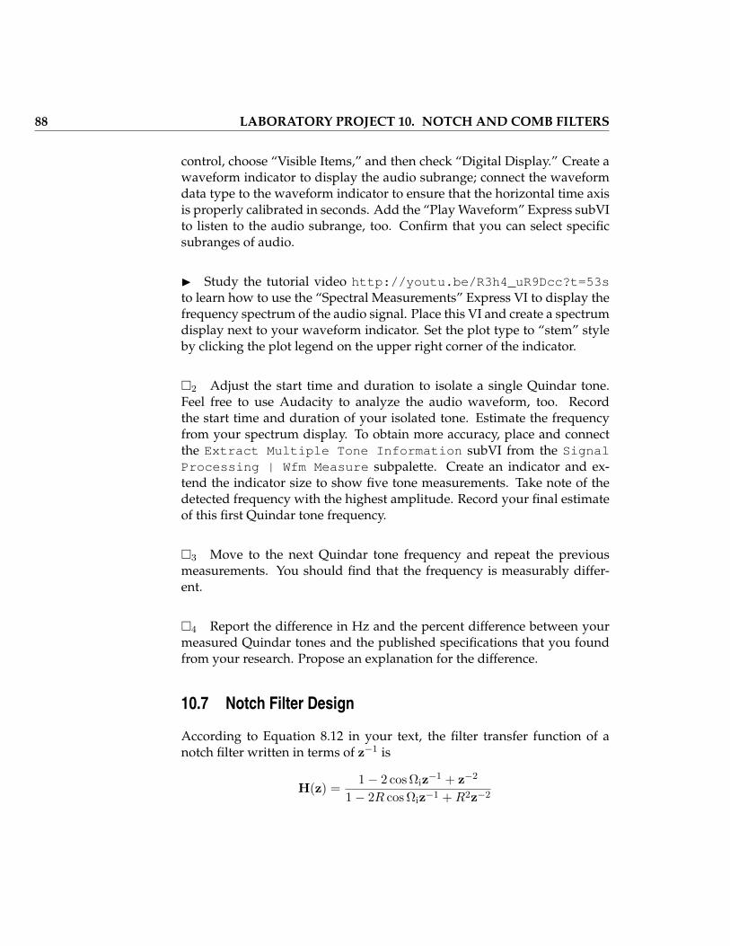
88 LABORATORY PROJECT 10. NOTCH AND COMB FILTERS
control, choose “Visible Items,” and then check “Digital Display.” Create awaveform indicator to display the audio subrange; connect the waveformdata type to the waveform indicator to ensure that the horizontal time axisis properly calibrated in seconds. Add the “Play Waveform” Express subVIto listen to the audio subrange, too. Confirm that you can select specificsubranges of audio.
I Study the tutorial video http://youtu.be/R3h4_uR9Dcc?t=53sto learn how to use the “Spectral Measurements” Express VI to display thefrequency spectrum of the audio signal. Place this VI and create a spectrumdisplay next to your waveform indicator. Set the plot type to “stem” styleby clicking the plot legend on the upper right corner of the indicator.
2 Adjust the start time and duration to isolate a single Quindar tone.Feel free to use Audacity to analyze the audio waveform, too. Recordthe start time and duration of your isolated tone. Estimate the frequencyfrom your spectrum display. To obtain more accuracy, place and connectthe Extract Multiple Tone Information subVI from the SignalProcessing | Wfm Measure subpalette. Create an indicator and ex-tend the indicator size to show five tone measurements. Take note of thedetected frequency with the highest amplitude. Record your final estimateof this first Quindar tone frequency.
3 Move to the next Quindar tone frequency and repeat the previousmeasurements. You should find that the frequency is measurably differ-ent.
4 Report the difference in Hz and the percent difference between yourmeasured Quindar tones and the published specifications that you foundfrom your research. Propose an explanation for the difference.
10.7 Notch Filter Design
According to Equation 8.12 in your text, the filter transfer function of anotch filter written in terms of z−1 is
H(z) =1− 2 cos Ωiz
−1 + z−2
1− 2R cos Ωiz−1 +R2z−2

10.7. NOTCH FILTER DESIGN 89
where Ωi = 2π(fi/fs), fi is the interfering tone frequency in Hz, and fs isthe sampling frequency, also in Hz. The numerator places a zero on theunit circuit at frequency Ωi while the denominator places a pole just insidethe unit circle at the same frequency; the constant R is the radial distancefrom the origin to the pole, and filter stability requires |R| < 1.
5 Design one notch filter for each Quindar tone; call these H1(z) andH2(z). Use the same filter constant R for both notch filters.
6 Cascade the two notch filters to create a single system function H(z) =H1(z)H2(z); expand the products of the numerator and denominator poly-nomials to obtain a ratio of two polynomials.
I Create a MathScript structure that accepts the audio sampling frequency,filter constantR, and two Quindar tone frequencies as inputs and producesthe difference equation a and b coefficient arrays. The tutorial video http://youtu.be/IsbItFzzOdA shows how to translate a transfer functionH(z) into a MathScript structure that in turn feeds the coefficient inputs ofthe digital filter subVI IIR Filter. Note that the MathScript convolutionfunction conv conveniently calculates the numerator and denominator co-efficient arrays of H(z) given the individual H1(z) and H2(z) arrays.
7 Place the Plot Pole-Zero and Plot Frequency Response VIs(available at https://decibel.ni.com/content/docs/DOC-24032and https://decibel.ni.com/content/docs/DOC-24021) and con-nect these to the outputs of your MathScript structure. Study the video tu-torials http://youtu.be/S8WmBxIlnEc and http://youtu.be/IsjXautfUXsto learn how to use these subVIs. Create default indicators for the fre-quency response magnitude and pole-zero plots. Capture a screen shotof these two indicators for your filter system function H(z). Confirm thatthe poles and zeros appear in the correct locations (zeros on the unit cir-cle, poles just inside the unit circle), and also confirm that the frequencyresponse goes to zero at the correct frequency.
I Place the IIR Filter subVI from the Signal Processing | Filters| Advanced IIR subpalette. Connect your a coefficients to the ReverseCoefficients input and your b coefficients to the Forward Coefficientsinput. Insert the filter just before your waveform and spectrum displays
90 LABORATORY PROJECT 10. NOTCH AND COMB FILTERS
and the audio player. Include a Boolean control to selectively enable the fil-ter, i.e., include a bypass path and a Select node from the Programming| Comparison subpalette.
8 Adjust the audio subrange start and duration times to your first Quin-dar tone. Collect screen shots of the spectrum with and without the notchfilter enabled. Turn off the vertical axis auto-scaling to use a common am-plitude scale. Report the amount by which the Quindar tone spectral com-ponent is reduced.
9 Repeat for the second Quindar tone.
I Study the tutorial video http://youtu.be/unuRYWUYQy4 to learnhow to temporarily disable a portion of the block diagram with a DiagramDisable structure, much as you would “comment out” a portion of code ina text-based programming language. Place the two spectrum-related VIsinside the Diagram Disable structure, and disable them for very long dura-tion subregions, e.g., greater than 45 s. The spectrum-related VIs consumetoo much memory when the subregion is long.
10 Now, extend the duration to critically listen to a longer audio clip;record the start and duration times. Experiment with values of R, start-ing with a value of 0.9. Discuss the degree to which the single notch filtersuppresses the Quindar tone sound.
11 Capture a screen shot of the waveform and spectrum displays for thelonger audio clip with and without filtering.
10.8 Comb Filter Design
You most likely can hear some harmonic residue of the Quindar tones, evenwith the notch filters engaged. In this section you will extend the notchfilter to a comb filter to deal with these harmonics, also called overtones.
12 Create new spectrum plots similar to those that you collected earlierfor the individual Quindar tones, and enable the notch filter. Look for thesecond harmonic (at twice the frequency of the fundamental) and estimateits amplitude as a percentage of the fundamental’s amplitude.

10.9. DISCUSSION 91
I Extend your MathScript structure to add two more notch filters at pre-cisely twice the frequencies of the two existing notch filters.
13 Capture a screen shot of the pole-zero diagram and frequency re-sponse indicators for your comb filter system function.
14 Set the start and duration times to those of your earlier critical listen-ing study. Experiment with different values of R; try to find the highestvalue that just causes the Quindar tones to become inaudible, and then re-port this value. Discuss the degree to which the comb filter suppresses theQuindar tone sound.
15 Capture a screen shot of the waveform and spectrum displays for thelonger audio clip with comb filtering enabled.
16 Select an audio subregion of approximately 15 s duration that demon-strates the effectiveness of your comb filter. Create one .wav file with thefilter disabled, and a second .wav file with the filter enabled. Submit thesetwo files as part of your deliverables.
10.9 Discussion
17 Discuss the overall performance of your two filter designs (notch andcomb).

92 LABORATORY PROJECT 10. NOTCH AND COMB FILTERS
Laboratory Project 11
Image Deblurring
11.1 Synopsis
Photographic image capture requires a finite amount of time to gather suffi-cient light energy to expose the image sensor. Relative motion between thecamera and the subject during exposure causes motion blur that smearsimage details. To the casual observer the blur renders the captured imageuseless. However, deconvolution of the blurring mechanism can recover aclose approximation of the original non-blurred image.
In this project you will be presented with an image that suffers fromuniform motion blur, the special case of constant relative velocity betweenthe camera and subject. With knowledge of the blurring mechanism youwill create and implement an inverse filter to deblur the image.
Ulaby/Yagle Section 8-4
11.2 Objectives
1. Work with image files; process and display images
2. Estimate motion blur with a mouse cursor measurement
3. Implement a stable inverse filter for a non-minimum phase system
4. Deblur an image with deconvolution

94 LABORATORY PROJECT 11. IMAGE DEBLURRING
11.3 Deliverables
1. Hardcopy of all LabVIEW block diagrams and front panels that youcreate
2. Screen shots of requested images and plots
3. Deblurred image file (PNG format)
4. Lab report or notebook formatted according to instructor’s require-ments
11.4 Required Resources
1. NI LabVIEW with MathScript RT Module
2. Blurred image supplied by instructor (PNG format)
11.5 Preparation
Image handling in LabVIEW
Images are two-dimensional signals with horizontal and vertical dimen-sions. LabVIEW can work with images as either 2-D or 1-D arrays. For thesake of simplicity in this project the image signal will be treated as a 1-Dsignal — much like an audio signal — in which the image rows are laidend to end beginning at the top of the image. In this scheme the first arrayelement is the upper left corner image pixel and the last array element isthe lower right corner image pixel.
I Study the tutorial video http://youtu.be/Z_81P1d_rCg on imagehandling in LabVIEW; topics include reading and writing PNG image files,image display, obtaining image information, and extracting the image pix-els as a 1-D array. You need only watch through time 5:00.
I Study the tutorial video http://youtu.be/pw7-smkZh_U to learnhow to make the picture indicator automatically size itself to the image.
11.6. INVERSE FILTER DESIGN 95
Image blurring
Your instructor has supplied you with a blurred image of a subject thatwas originally sharp and detailed. The blurred image resulted from uni-form motion in the horizontal direction by an unknown distance of D pix-els where D is an integer. Uniform motion blur is identical to the mov-ing average (MA) system described in Section 7-3.4 of your text; see Equa-tion 7.34 for the difference equation of the MA system. Substituting blur-ring distance D for the constant M , setting the bi coefficients to 1, and z-transforming this equation leads to the blurring system
H(z) =1
D + 1
D∑i=0
z−i. (11.1)
Dividing by D + 1 ensures that the system has unity DC gain to keep theblurred image at the same average intensity as the original image.
Image analysis
The motion blur distance can be estimated by measuring the length ofstreaks traced out by the blur of small but distinct features.
I Create a new LabVIEW VI as a starting point for your image analysisapplication, and then load and display the blurred image provided by yourinstructor.
I Study the tutorial video http://youtu.be/nVIOnz2WYyQ to learnhow to display mouse coordinates. Note that the while-loop and eventstructure need not enclose your existing code that reads the PNG image,but should instead be placed in its own area of the block diagram.
1 Update your VI to implement the mouse coordinate display, and thenestimate and report the blurring distance D.
11.6 Inverse Filter Design
The inverse filter (also called image deblurring filter) seeks to undo the ef-fects of the image blurring filter. The inverse filter G(z) satisfies the prop-erty G(z)H(z)=1.

96 LABORATORY PROJECT 11. IMAGE DEBLURRING
Basic inverse filter
I Create a new LabVIEW VI as a starting point for your image deblurringapplication, and then load and display the blurred image provided by yourinstructor.
2 Study the tutorial video http://youtu.be/JJZ-shHiayU to learnhow to write the blurring system H(z) (Equation 11.1 on the precedingpage) in closed form, i.e., without a summation symbol.
3 Write the inverse filter system G(z) for your closed-form version ofH(z).
I Study the video http://youtu.be/IsbItFzzOdA to learn how totranslate a system transfer function into a MathScript structure; also studythe section near the end of the video that shows how to connect the fil-ter coefficient arrays for the a and b coefficient arrays to the LabVIEWIIR_Filter.vi subVI.
I Implement the system G(z) as a MathScript structure. Create an inputfor pixel distanceD and two outputs for the a and b filter coefficient arrays.The MathScript zeros function comes in handy to implement the denom-inator coefficients; use the form zeros(1,N) to create a 1-D array of zerosof length N .
4 Place the Plot Pole-Zero and Plot Frequency Response VIs(available at https://decibel.ni.com/content/docs/DOC-24032and https://decibel.ni.com/content/docs/DOC-24021) and con-nect these to the outputs of your MathScript structure for G(z). Study thevideo tutorials http://youtu.be/S8WmBxIlnEc and http://youtu.be/IsjXautfUXs to learn how to use these subVIs. Create default indi-cators for the frequency response magnitude and pole-zero plots of G(z).Study the effect of blurring distance D on the two plots and discuss yourobservations.
5 Where are the poles of G(z) located in the pole-zero diagram? Howdo these pole locations manifest themselves in the frequency response plot?

11.7. IMAGE DEBLURRING 97
Stable inverse filter
The basic inverse filter G(z) is not BIBO stable because the image blur-ring system H(z) is not minimum phase. Pulling the poles of G(z) slightlyinside the unit circle makes the deblurring filter stable at the expense ofintroducing a slight mismatch between the original blurring filter and itsinverse filter.
6 Apply z-transform property #5 (“Multiplication by an”, also knownas the z-scaling property) of Table 7-6 in your text to G(z) by substitutingeach instance of z with z/R to form the stable inverse filter GS(z) where Ris the pole radius with |R| < 1.
I Update the MathScript structure to create the filter coefficients for GS(z);add an additional input for R.
7 Plot the pole-zero diagram and frequency response of GS(z). Investi-gate values of R in the vicinity of 1.
Unit DC gain
The inverse filter requires a DC gain of 1 to ensure that the average bright-ness of the deblurred image remains the same as the original image.
8 Calculate the DC gain of GS(z), i.e., evaluate GS(z) at z = ej0 = 1.
I Update the MathScript structure to divide the existing GS(z) by the DCgain you calculated in the previous step, thereby ensuring that GS(z) hasunit DC gain for all values of D and R.
11.7 Image Deblurring
I Use the IIR_Filter.vi and the a and b coefficients produced byyour MathScript structure to calculate the deblurred image.
I Place your deblurring system inside a combined event-structure andwhile-loop structure so that you can interactively adjust the blurring dis-tance D and the pole radius R while observing the deblurred image. Referto the tutorial video http://youtu.be/eGlvOiqYVxg for details.

98 LABORATORY PROJECT 11. IMAGE DEBLURRING
I Begin with D set to your estimated blur distance and R set to 0.95.Iteratively adjust both parameters to deblur the image to the best of yourability. Strive for sharp (non-blurry) features, low noise, and minimumartifacts.
I Study the tutorial video http://youtu.be/IDVHarNkJSU to learnhow to modify your event structure to save your image results to a filewhen you stop the while-loop. The video describes a general-purpose load–process–save design pattern that applies to a wide variety of signal process-ing tasks.
9 Save your deblurred image as a PNG file, and report the values of Dand R for this image.
11.8 Discussion
10 Discuss your results, especially the nature of the noise and artifacts,and their relation to the parameters R and D. Consider including addi-tional example images in your report to substantiate your discussion.
11 Explain how the original image blurring process actually removessome information from the image, and how this impacts the design of thedeblurring filter.

Laboratory Project 12
DTMF Decoder
12.1 Synopsis
Listen to the sound of your telephone keypad when you dial a number.These distinctive sounds known as DTMF tones provide a way for yourphone to communicate dialing information to the telephone switching sys-tem. No doubt you are familiar with the numbers 0 to 9 and the asteriskand pound keys; the DTMF standard defines four additional keys to pro-vide 16 unique tones altogether.
In this project you will create a complete DTMF decoder system basedon FFT spectral analysis. Your decoder system will accept an audio record-ing of a DTMF tone sequence as input and display the detected tones on agrid of visual indicators.
Ulaby/Yagle Sections 8.6–8.7
12.2 Objectives
1. Interpret a signal’s magnitude spectrum to search for periodic signals
2. Investigate windowing as a means to reduce spectral leakage
3. Process audio signals and work with audio files
4. Implement an edge detector to automatically identify the location ofDTMF tone bursts in an audio waveform

100 LABORATORY PROJECT 12. DTMF DECODER
12.3 Deliverables
1. Hardcopy of all LabVIEW block diagrams and front panels that youcreate
2. Screen shots of requested spectrum/time plots
3. Lab report or notebook formatted according to instructor’s require-ments
12.4 Required Resources
1. NI LabVIEW with MathScript RT Module
2. Audio file of a mystery DTMF digit sequence provided by instructor
12.5 Preparation
DTMF decoder block diagram
Figure 12.1 shows the high-level block diagram of the DTMF decoder sys-tem that you will create in this project. The decoder loads an audio file thatcontains a DTMF tone sequence, extracts an audio subrange for a singletone, calculates the discrete Fourier transform (DFT) magnitude spectrumfor the tone, and decodes the spectral information to determine the corre-sponding DTMF digit.
Figure 12.1: High-level block diagram DTMF decoder system.
DTMF tones
Learn about DTMF tones and create your own audio test sequence.

12.5. PREPARATION 101
1 Do an Internet search to determine the following information aboutDTMF tones:
1. Meaning of the acronym “DTMF,”
2. The year in which telephones first began to use DTMF,
3. Labels of the 16-key DTMF keypad,
4. Frequencies of the keypad rows, and
5. Frequencies of the keypad columns.
Include URLs for the articles from which you obtained this information.
I Install the Audacity software available at http://audacity.sourceforge.net. Run Audacity to create a new project. Set the “Project Rate” (systemsampling frequency) to 8 kHz; see the lower left corner of the application.Select the menu command Generate | DTMF Tones and then enter thefollowing information into the dialog box:
• “DTMF Sequence” = 123A456B789C*0#D,
• “Amplitude” = 0.8,
• “Duration” = 5 seconds, and
• “Tone/silence ratio” = 50% (you will see a tone duration of 161 mswith these settings).
Select File | Export to save the audio as a WAV 16-bit audio file.
I Alternatively, search for a web service that converts the DTMF digitsand letters to a .wav audio file, e.g., http://www.dialabc.com/sound/generate. Remember to select 8 kHz for the sampling frequency.
DFT-based spectral analysis
In this project you will use DFT spectral analysis as the heart of your DTMFdecoder.
I Study Sections 8-6 and 8-7 in your text.
102 LABORATORY PROJECT 12. DTMF DECODER
I Study the tutorial video at http://youtu.be/z7X6jgFnB6Y for anoverview of DFT spectral analysis.
I Study the tutorial video at http://youtu.be/UGUceuhSuUE to learnmore about the relationship between the time-domain waveform and itsfrequency-domain spectrum computed by the fast Fourier transform (FFT)algorithm. Note that the terms “DFT” and “FFT” are often used inter-changeably.
12.6 Spectral Analysis
In this section you will analyze individual DTMF tones to better under-stand how to design your DTMF decoder.
I Create an empty top-level VI to serve as the starting point of yourDTMF decoder application.
I Follow along with the video http://youtu.be/ChSVf9lZ44k tolearn how to read a .wav audio file, extract the 1-D signal array, and playthe audio to your soundcard. Use the DTMF test sequence audio you cre-ated earlier.
I Add block diagram code to calculate the audio file length in secondsand the sampling rate in Hz, and display these values on the front panel.
I Create a waveform indicator to display the complete audio signal.
I Study the help page for “Array Subset.” Add controls to specify thestart time (in seconds) and the length N (in samples – note the difference)of a subrange of audio. The “Horizontal Pointer Slide” control style workswell. Enable the digital display for fine control of the desired time andsample values; right-click on the control, choose “Visible Items,” and thencheck “Digital Display.”
I Use “Build Waveform” to convert the 1-D array subset to waveformdatatype, and connect the waveform data type to a new waveform indica-tor that displays the audio subrange; ensure that the horizontal time axis isproperly calibrated in seconds. Re-connect the “Play Waveform” Express

12.6. SPECTRAL ANALYSIS 103
subVI to listen to the audio subrange instead of the complete signal. Con-firm that you can select any desired audio subrange.
I Study the tutorial video http://youtu.be/9SL5_jY87IA to learnhow to use the “FFT” built-in subVI located in the Signal Processing| Transforms subpalette. Place and connect this VI to your audio sub-range; use the same subrange length control value for the FFT length.
I Add an “Array Subset” node to extract the lower half of the FFT outputarray (the upper half contains a mirror image of the lower half and does notneed to be plotted).
I Divide the FFT output by the subrange length N to normalize the val-ues.
I Place a “Complex to Polar” node from the Programming | Numeric| Complex subpalette to compute the FFT magnitude, and then displaythis array on a waveform plot. Set the plot type to “stem” style by clickingthe plot legend on the upper right corner of the indicator. Turn off auto-scaling on the Y axis and set the maximum value to 0.12.
2 Set the subrange length to 128, and then adjust the start time to isolatea single DTMF tone. Run the VI to see the tone’s waveform and spectrum,and also to listen to the tone. Create a screenshot of the spectrum and statethe associated DTMF tone digit. Discuss the appearance of the DFT spec-trum.
3 Repeat the previous step for another DTMF tone, noting the differ-ences that appear in the DFT spectrum.
4 Try increasing the FFT length to values 256, 512, and 1024; note thatthe FFT algorithm works most efficiently with array lengths that are a powerof two. Discuss all effects that you observe resulting from longer FFTlengths.

104 LABORATORY PROJECT 12. DTMF DECODER
5 Derive an equation to calculate the FFT spectral bin number for agiven frequency f0. Recall that the bin number is an integer. Calculate thefrequency bin numbers for the two DTMF frequencies for a selected DTMFtone digit withN = 1024. Zoom in on the spectral lines in the spectrum plot(right-click on the waveform graph indicator, enable the “Graph Palette”option of “Visible Items,” and then use the zoom controls). Create a screenshot of the zoomed plot and mark up the screenshot to demonstrate thatyour equation properly calculates the FFT bin number for a given DTMFfrequency.
I Note the abundance of spectral lines that cluster around the base ofthe tall spectral line that corresponds to each DTMF frequency. This spec-tral leakage effect can be reduced by windowing the waveform array be-fore it is applied to the FFT. Study the tutorial video http://youtu.be/UGUceuhSuUE to learn more about spectral leakage and windowing.
6 Select the Hamming window subVI from the Signal Processing| Windows subpalette and insert this before the FFT. Discuss the reductionin spectral leakage that you observe.
12.7 Tone Detector and Display
By now you have developed a good feel for the spectral representation ofDTMF tones, and you also know how to translate any particular DTMFtone frequency to an FFT bin number. In this section you will complete thetone detector and display panel.
7 Determine a suitable threshold to distinguish between the presenceand absence of all 32 DTMF tone frequencies. Use a “Greater?” node fromthe Programming | Comparison subpalette to threshold the FFT mag-nitude array; use a front-panel control for the threshold value. Report thethreshold value you selected.
I Use the “Index Array” node from the Programming | Array sub-palette to extract the thresholded frequency bins of the four DTMF keypadrow frequencies; pull on the bottom handle of “Index Array” to create fourindex inputs and outputs. Create four constants for the DTMF keypad rowfrequencies (in Hz) and then add additional mathematical nodes to convert

12.8. COMPLETE DTMF DECODER 105
the frequencies to bin numbers for the “Index Array” inputs. In this wayyour DTMF decoder will work properly for any subrange length N thatyou choose. The end result of this step is four Boolean wires that indicatewhich DTMF keypad row is active, if any.
I Repeat the previous step to create four Boolean wires for the DTMFkeypad columns. Arrange your block diagram layout to make a 4-by-4grid of Boolean wires.
I The Boolean “AND” gate uniquely detects the two frequencies for agiven DTMF digit. Use sixteen AND gates from the Programming | Booleansubpalette placed at the intersections of the row and column Boolean wires.Create a Boolean indicator at the output of each AND gate. Label the in-dicators according to the sixteen DTMF digits and arrange the front-panelindicators in the shape of a standard DTMF keypad.
I Test your finished tone decoder display for each of the sixteen DTMFtones in your audio test sequence.
12.8 Complete DTMF Decoder
At this point in the project you have demonstrated that your design cansuccessfully detect each of the sixteen DTMF tones in an audio sequence.However, you must manually set the start position of each tone. In thissection you will add an edge detector to automatically find the leading edgesof all of the DTMF tone bursts and then loop over all of the tone burstsdetected in the audio signal.
Figure 12.2 on the following page shows the block diagram of the DTMFdecoder system with a tone-burst edge detector to automatically identifythe starting index of each tone burst in the sequence. The edge detectorcreates an array of start times that control a for-loop structure to repeatedlyrun the block diagram that you have developed so far.
I Enter the edge detector block diagram code shown in Figure 12.3 onthe next page. The edge detector consists of an envelope detector, compara-tor, differentiator, and threshold detector. Place the needed components bytyping “Ctrl+Space” for the “Quick Drop” menu and typing the followingnames:
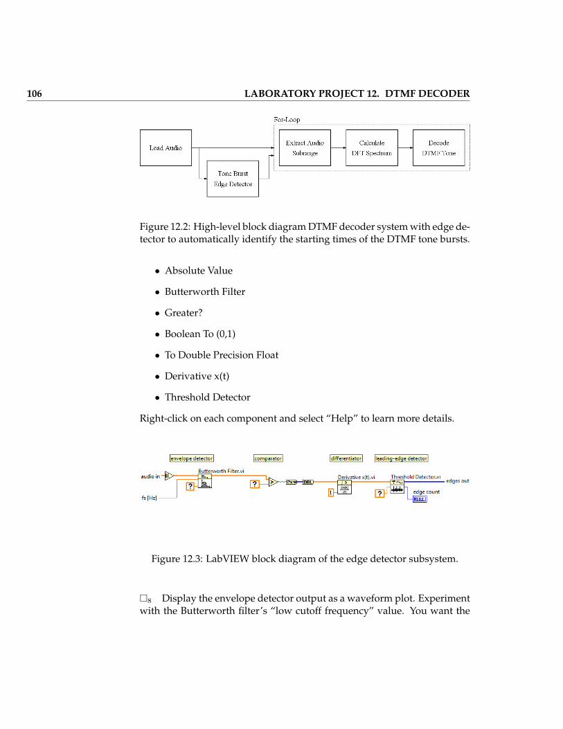
106 LABORATORY PROJECT 12. DTMF DECODER
Figure 12.2: High-level block diagram DTMF decoder system with edge de-tector to automatically identify the starting times of the DTMF tone bursts.
• Absolute Value
• Butterworth Filter
• Greater?
• Boolean To (0,1)
• To Double Precision Float
• Derivative x(t)
• Threshold Detector
Right-click on each component and select “Help” to learn more details.
Figure 12.3: LabVIEW block diagram of the edge detector subsystem.
8 Display the envelope detector output as a waveform plot. Experimentwith the Butterworth filter’s “low cutoff frequency” value. You want the

12.9. DISCUSSION 107
filter output to accurately track the outline (envelope) of the DTMF tonebursts. Create a screen shot of the envelope detector output and report thefinal value you selected for the cutoff frequency.
9 Display the comparator output as a waveform plot. Select a thresholdvalue that produces a clean squarewave representation of the DTMF toneburst envelope. Create a screen shot of the comparator output and reportthe final value you selected for the threshold value.
10 Display the differentiator output as a waveform plot; create a screenshot of the plot.
11 Add the “Threshold Detector” to determine the index values of theleading edges of the tone bursts. Select a threshold value to detect leadingedges only; report your final value. Create an indicator for the “count”output to display the number of detected edges.
I Determine which parts of the existing block diagram to enclose in afor-loop structure. Wire the output of the “Threshold Detector” subVI intothe for-loop structure using the default “Auto-Indexed Tunnel;” in this waythe loop will execute one time for each DTMF tone burst. Include a “Wait”in the for-loop to set the pace of the tone playback and display.
I Test your complete DTMF decoder with your own audio test sequenceand confirm that it works properly.
12 Run your decoder with the instructor’s mystery DTMF sequence. Re-port the DTMF digit sequence you discovered.
12.9 Discussion
13 Discuss the overall performance of your DTMF decoder system.

108 LABORATORY PROJECT 12. DTMF DECODER

Appendix A
Parts List
Resistors
The following resistors are standard-value 5% tolerance 1/4 watt carbonfilm devices. All listed resistors are available in resistor kits from Digi-Key,Jameco, and RadioShack with the following exceptions: (1) the Digi-Key kitdoes not contain a 10 MΩ resistor, and (2) none of the kits contain a 2 MΩresistor (this can be created with two series-connected 1 MΩ resistors):
Resistor Kit Description Supplier Part #365 pcs, 5 ea of 1.0Ω to 1.0MΩ Digi-Key RS125-ND540 pcs, 30 values, 10Ω to 10MΩ Jameco 103166500 pcs, 64 values, 1.0Ω to 10MΩ RadioShack 271-312
See Resistor Color Codes at http://www.allaboutcircuits.com/vol_5/chpt_2/1.html to learn how to read the color bands on carbon filmresistors.
Qty Value (kΩ) Color Code4 1.0 Brown - Black - Red1 10 Brown - Black - Orange2 15 Brown - Green - Orange
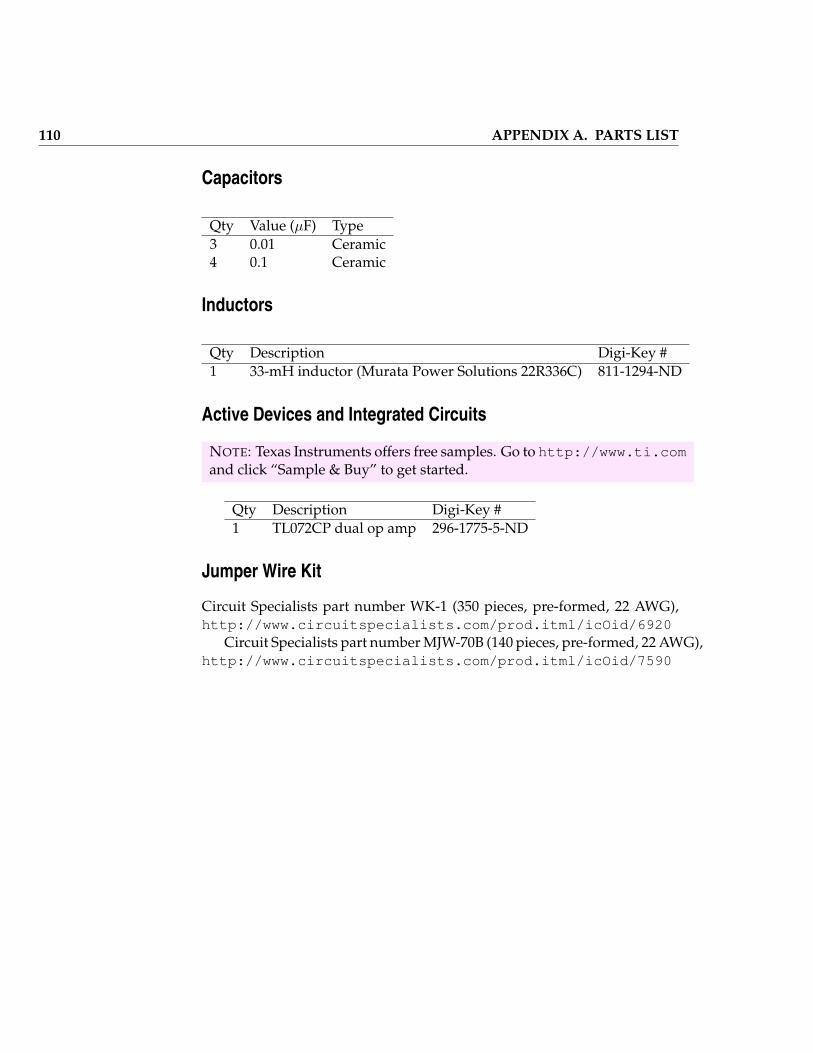
110 APPENDIX A. PARTS LIST
Capacitors
Qty Value (µF) Type3 0.01 Ceramic4 0.1 Ceramic
Inductors
Qty Description Digi-Key #1 33-mH inductor (Murata Power Solutions 22R336C) 811-1294-ND
Active Devices and Integrated Circuits
NOTE: Texas Instruments offers free samples. Go to http://www.ti.comand click “Sample & Buy” to get started.
Qty Description Digi-Key #1 TL072CP dual op amp 296-1775-5-ND
Jumper Wire Kit
Circuit Specialists part number WK-1 (350 pieces, pre-formed, 22 AWG),http://www.circuitspecialists.com/prod.itml/icOid/6920
Circuit Specialists part number MJW-70B (140 pieces, pre-formed, 22 AWG),http://www.circuitspecialists.com/prod.itml/icOid/7590
Appendix B
TL072 Operational Amplifier
The Texas Instruments TL072 dual operational amplifier (“op amp”) pro-vides two op amp devices in a single 8-pin package. For more detailssee the datasheet available at http://www.ti.com; enter “tl072” in the“Search by Part Number” field.
Figure B.1 on the following page shows the pinout diagram for theTL072. Note the requirement for a dual power supply; the NI NI ELVISII ±15 V supply serves this purpose. Also note that the op amp device it-self does not have a ground terminal. Instead the NI ELVIS II GROUND(analog ground) establishes the ground reference.
NI Multisim provides a circuit model for the TL072: place the TL072CPdevice.

112 APPENDIX B. TL072 OPERATIONAL AMPLIFIER
Figure B.1: Texas Instruments TL072 dual op amp pinout diagram (topview). The plastic package uses either a U-shaped cutout to indicate theleft side or an indented circle to indicate pin 1. NOTE: In this book thepositive supply “VCC+” is called VCC and the negative supply “VCC-” iscalled VEE.
Appendix C
Video Tutorial Links
Signals and Systems Concepts
• Work through a complete graphical convolution example:http://youtu.be/zoRJZDiPGds
• Understand discrete-time convolution with an example:http://youtu.be/yyTu0SXeW1M
• Study the Butterworth filter magnitude response:http://youtu.be/QJdNVdL4iBQ
• Apply the 2-D FFT as an image filter:http://youtu.be/X53SrMnu91A
• Create a 2-D Butterworth image filter:http://youtu.be/qpwUHt-DEbs
NI LabVIEW Video Tutorials
General-purpose techniques:
• Configure “look and feel” of LabVIEW 2012:http://youtu.be/M6gDpso6ysI
• Create a subVI:http://youtu.be/C2zYeC_RpM8
• Create a load-process-save design pattern:http://youtu.be/IDVHarNkJSU

114 APPENDIX C. VIDEO TUTORIAL LINKS
• Display mouse coordinates:http://youtu.be/nVIOnz2WYyQ
• Disable a portion of block diagram code:http://youtu.be/unuRYWUYQy4
• Use global variables to reduce wiring clutter:http://youtu.be/PquslTj69f4
• Create a menu control:http://youtu.be/tImN4C03W1k
• Create an interactive front panel with event structure:http://youtu.be/eGlvOiqYVxg
• Execute an event structure one time on run:http://youtu.be/UFEvmmggqLQ
Digital filtering:
• Use the “Convolution” subVI:http://youtu.be/Fsf88Rmimz4
• Create a bandpass filter subVI:http://youtu.be/gBVluWy_UGs
• Implement H(z) as a digital filter:http://youtu.be/IsbItFzzOdA
• Use the “Plot Frequency Response” subVI:http://youtu.be/IsjXautfUXs
• Use the “Plot Pole-Zero” subVI:http://youtu.be/S8WmBxIlnEc
Audio:
• Work with .wav audio files:http://youtu.be/ChSVf9lZ44k
• View an audio signal and its spectrum:http://youtu.be/R3h4_uR9Dcc

115
Images:
• Basic image handling techniques:http://youtu.be/Z_81P1d_rCg
• Auto-resize an image picture indicator:http://youtu.be/pw7-smkZh_U
Fast Fourier Transform (FFT):
• Compute magnitude spectrum with the “FFT” subVI:http://youtu.be/9SL5_jY87IA
• Demonstrate basic properties of the FFT:http://youtu.be/UGUceuhSuUE
• Study the basic concepts of the FFT:http://youtu.be/z7X6jgFnB6Y
NI LabVIEW MathScript Video Tutorials
• Get started with the MathScript Window:http://youtu.be/Tvi1oY0lV2g
• Plot two functions of time:http://youtu.be/XQlAai1-YVc
• Take cursor measurements on a plot:http://youtu.be/bgK1p5O6OXc
• Work with images in the MathScript Window:http://youtu.be/oM_KSYIDrE4
NI Multisim & NI ELVISmx Video Tutorials
• Compare simulated and physical DMM measurements:http://youtu.be/MZiZ_C-ngkY

116 APPENDIX C. VIDEO TUTORIAL LINKS
NI Multisim Video Tutorials
Place components:
• Find commonly-used circuit components:http://youtu.be/G6ZJ8C0ja9Q
• Find components by name:http://youtu.be/5wlFweh4n-c
• Place and operate linear potentiometer:http://youtu.be/oazwGLzWvhs
• Place dual op amp second device:http://youtu.be/-QDFEf-KdEw
Sources:
• Function generator:http://youtu.be/CeOl6EzD-_c
• AC (sinusoidal) voltage source:http://youtu.be/CXbuz7MVLSs
• ABM (Analog Behavioral Model) voltage source:http://youtu.be/8pPynWRwhO4
• Pulse voltage source:http://youtu.be/RdgxVfr28C8
• Piecewise linear (PWL) voltage source:http://youtu.be/YYU5WuyebD0
• VDD and VSS power supply voltages:http://youtu.be/XrPVLgYsDdY
• VCC and VEE power supply voltages:http://youtu.be/XkZTwKD-WjE
Measure DC power:
• Use a Parameter Sweep analysis to plot resistor power as a functionof resistance:http://youtu.be/3k2g9Penuag

117
Measure frequency response:
• Measure frequency response with AC Analysis:http://youtu.be/tgCPDBtRcso
Net names:
• Display and change net names:http://youtu.be/0iZ-ph9pJjE
Grapher View and oscilloscope cursor measurements:
• Find the maximum value of a trace in Grapher View:http://youtu.be/MzYK60mfh2Y
• Set cursor to a specific value:http://youtu.be/48sQja58I10
Grapher View environment:
• Add data label to Grapher View plot:http://youtu.be/uibNqFlod_Y
• Plot mathematical expression:http://youtu.be/qYVf_rkTF-o
• Adjust axis limits and tick marks on a Grapher View plot:http://youtu.be/nxHHMpJd5Ow
• Plot second variable on its own axis in Grapher View:http://youtu.be/rULFKRTphcI
• Export simulation data to an Excel spreadsheet:http://youtu.be/s6ezjb8Xrhc
Oscilloscope:
• Basic operation of the two-channel oscilloscope:http://youtu.be/qnRK6QyqjvQ
• Waveform cursor measurements with the two-channel oscilloscope:http://youtu.be/snBRFq1Y1q4

118 APPENDIX C. VIDEO TUTORIAL LINKS
• Distinguish oscilloscope traces by color:http://youtu.be/bICbjggcTiQ
• Stabilize the oscilloscope display with edge triggering:http://youtu.be/d69zYYSEG7E
• Basic operation of the four-channel oscilloscope:http://youtu.be/iUqs_c1Bc4Y
Transient response:
• Plot time-domain circuit response with Transient Analysis:http://youtu.be/waKnad_EXkc
Combined Multisim / ELVISmx measurements:
• Combine Multisim simulation and myDAQ measurements in the sameinstrument – Bode Analyzer:http://youtu.be/3UmTmUj4h1g
NI ELVISmx Video Tutorials
See Electrical Circuits with NI myDAQ for more video tutorials and projects:http://decibel.ni.com/content/docs/DOC-12654
NI ELVISmx Instruments:
• DMM ohmmeter:http://decibel.ni.com/content/docs/DOC-12938
• DMM voltmeter:http://decibel.ni.com/content/docs/DOC-12937
• DMM ammeter:http://decibel.ni.com/content/docs/DOC-12939
• Function Generator (FGEN):http://decibel.ni.com/content/docs/DOC-12940
• Arbitrary Waveform Generator (ARB):http://decibel.ni.com/content/docs/DOC-12941

119
• Oscilloscope:http://decibel.ni.com/content/docs/DOC-12942
• Bode Analyzer:http://decibel.ni.com/content/docs/DOC-12943
• Digital Reader (DigIn):http://decibel.ni.com/content/docs/DOC-12944
• Digital Writer (DigOut):http://decibel.ni.com/content/docs/DOC-12945
Measurement techniques:
• Increase current drive of analog output (AO) channels with an op ampvoltage follower:http://decibel.ni.com/content/docs/DOC-12665