c 2008 Xiaofeng Liu - Pennsylvania State...
183
c 2008 Xiaofeng Liu
Transcript of c 2008 Xiaofeng Liu - Pennsylvania State...

c© 2008 Xiaofeng Liu

NUMERICAL MODELS FOR SCOUR AND LIQUEFACTION AROUND OBJECT UNDERCURRENTS AND WAVES
BY
XIAOFENG LIU
B.Eng., Tsinghua University, 2000M.Eng., Peking University, 2003
M.S., University of Illinois at Urbana-Champaign, 2007
DISSERTATION
Submitted in partial fulfillment of the requirementsfor the degree of Doctor of Philosophy in Civil Engineering
in the Graduate College of theUniversity of Illinois at Urbana-Champaign, 2008
Urbana, Illinois
Doctoral Committee:
Professor Marcelo H. Garcıa, ChairProfessor Gary ParkerProfessor Albert ValocchiAssociate Professor Arif MasudDr. Robert R. Holmes, Jr., USGS Illinois Water Science Center

Abstract
Local scour and liquefaction are two of the most important processes which affect the interactions
between fluid, object and sediment when an object (such as bridge pier, offshore foundation, etc.) is
exposed to currents and waves. In the present study, numerical models are developed to understand
these complicated processes.
For the local scour process, two-dimensional and three-dimensional models are developed re-
spectively. In the two-dimensional model, shallow water equations with finite volume method on
unstructured mesh are used. The two-dimensional model uses the Godunov scheme and approxi-
mate Riemann solvers. Hydrodynamics and sediment transport equations are coupled and solved
simultaneously. Asymptotic analysis of the system eigenvalues is given and the approximation is
compared with the numerical results. The model developed in this thesis can deal with wetting and
drying automatically. Discontinuity of the flow, such as a hydraulic jump, can be captured. For
the three dimensional model, free water surface and automatic mesh deformation for the bed are
incorporated in the model. The Reynolds Averaged Navier-Stokes (RANS) turbulence model is
used to simulate the turbulent flow field. The turbulence model used is k- ε Model. Two interfaces
(water and air, water and sediment) present in the domain are captured with different approaches.
The free surface of the flow is captured by Volume of Fluid (VOF) scheme which is an Eulerian
approach. A new method for the VOF scheme is proposed to reduce the computational time while
retaining relatively good accuracy. The water-sediment interface (bed) is captured with a mov-
ing mesh method which is a Lagrangian approach. Unlike the two-dimensional model, the flow
field is coupled with sediment transport (both bed load and suspended load) using a quasi-steady
approach. Numerical simulations are carried out and compared with experimental results. Good
ii

results are obtained with the proposed model. The flow field compares well with the experimental
observations. Scour patterns are similar to the experimental data. Long computational time is
needed for morphological simulation and parallel computation is used to accelerate this process.
Three-dimensional model can capture the detailed flow structure around an object and predict the
scour process more accurately. However, the two-dimensional model can be used as a fast assess-
ment tool for large computational domains.
For the liquefaction process, two different mechanisms (momentary and residual) are con-
sidered. For momentary liquefaction, a three-dimensional numerical model for the sea bed re-
sponse under free surface water waves is constructed. Free water surface is modeled by volume
of fluid (VOF) method and water waves are generated by numerical wave-maker boundary con-
dition. An iterative numerical scheme is proposed to solve the Biot consolidation equation using
a finite volume method (FVM). The coupling between water wave and sea bed is through both
pressure and stress conditions on common boundaries. For residual liquefaction, the solutions to
the one-dimensional model equation of the period-averaged pore pressure buildup are listed. The
accumulation of pore pressure is modeled as the effect of the source term in the storage equation.
Corrections to the solutions in the literature are provided. For deep soil condition, an asymptotic
solution is proposed to estimate the pore pressure. A numerical model is also developed to solve
the one-dimensional period-averaged pore pressure buildup equation. Good agreement between
the results of numerical model and analytical model are found. These results also agree with the
experiment data. A tentative step is also made to model the phase-resolved pore pressure. The
basic idea of adding a source term to the governing equation is explored. The source term has the
same form as that of the period-averaged residual pore pressure model. Test case shows that this
model gives good results comparing to the one-dimensional period-averaged model.
iii

To My Family.
iv

Acknowledgments
This thesis would not have been possible without the support of many people. Firstly, I would like
to thank my advisor Professor Marcelo H. Gracıa for his support and valuable advices. Throughout
my doctoral work, he continually encouraged me to develop independent research skills. Special
thanks to the exceptional committee, Professors Gary Parker, Albert J. Valocchi, Arif Masud and
Robert R. Holmes Jr., who provided valuable suggestions regarding the topic of this dissertation.
Also, I extend many thanks to my colleagues and friends, especially Michael (Xuejun) Yang, Jorge
Abad, Javier Ancalle, Mariano I. Cantero, Robert Haydel, Blake Landry, Arturo S. Leon, Francisco
Pedocchi and Octavio Sequeiros. I am grateful to Andy Waratuke for helping me with lab issues.
Finally, thanks to my family for their constant support and love; without them, it would be very
difficult to complete this thesis.
This research was funded by the Coastal Geosciences Program of the U.S. Office of Naval Re-
search through the Grants N00014-01-1-0337. Supercomputer time was provided by the National
Center for Supercomputing Applications (NCSA) at UIUC. This support is gratefully acknowl-
edged.
v

Table of Contents
List of Tables . . . . . . . . . . . . . . . . . . . . . . . . . . . . . . . . . . . . . . . . . . ix
List of Figures . . . . . . . . . . . . . . . . . . . . . . . . . . . . . . . . . . . . . . . . . x
List of Abbreviations . . . . . . . . . . . . . . . . . . . . . . . . . . . . . . . . . . . . . xiii
List of Symbols . . . . . . . . . . . . . . . . . . . . . . . . . . . . . . . . . . . . . . . . . xiv
Chapter 1 Introduction . . . . . . . . . . . . . . . . . . . . . . . . . . . . . . . . . . . 11.1 Motivations . . . . . . . . . . . . . . . . . . . . . . . . . . . . . . . . . . . . . . 11.2 Objectives of This Research . . . . . . . . . . . . . . . . . . . . . . . . . . . . . 31.3 Methodology . . . . . . . . . . . . . . . . . . . . . . . . . . . . . . . . . . . . . 61.4 Outline of the Dissertation . . . . . . . . . . . . . . . . . . . . . . . . . . . . . . 7
Chapter 2 Two Dimensional Model for Scour Around Object Using Shallow WaterEquations on Unstructured Mesh . . . . . . . . . . . . . . . . . . . . . . . . . . . . . 82.1 Introduction . . . . . . . . . . . . . . . . . . . . . . . . . . . . . . . . . . . . . . 82.2 Governing Equations . . . . . . . . . . . . . . . . . . . . . . . . . . . . . . . . . 11
2.2.1 Shallow Water Equations . . . . . . . . . . . . . . . . . . . . . . . . . . . 112.2.2 Sediment Conservation and Transport Equations . . . . . . . . . . . . . . 12
2.3 Numerical Method of the Model . . . . . . . . . . . . . . . . . . . . . . . . . . . 132.3.1 Quasi-Steady Approach . . . . . . . . . . . . . . . . . . . . . . . . . . . 142.3.2 Coupled Approach . . . . . . . . . . . . . . . . . . . . . . . . . . . . . . 15
2.4 Evaluation of Numerical Fluxes . . . . . . . . . . . . . . . . . . . . . . . . . . . 152.4.1 Inviscid Fluxes . . . . . . . . . . . . . . . . . . . . . . . . . . . . . . . . 15
2.5 Asymptotic Analysis of the Wave Speeds . . . . . . . . . . . . . . . . . . . . . . 182.5.1 One-Dimensional System . . . . . . . . . . . . . . . . . . . . . . . . . . 192.5.2 Two-Dimensional System . . . . . . . . . . . . . . . . . . . . . . . . . . 202.5.3 Viscous Fluxes . . . . . . . . . . . . . . . . . . . . . . . . . . . . . . . . 26
2.6 Limiter for High Order Schemes . . . . . . . . . . . . . . . . . . . . . . . . . . . 262.7 Time Integration . . . . . . . . . . . . . . . . . . . . . . . . . . . . . . . . . . . . 282.8 Boundary Conditions . . . . . . . . . . . . . . . . . . . . . . . . . . . . . . . . . 28
2.8.1 Walls . . . . . . . . . . . . . . . . . . . . . . . . . . . . . . . . . . . . . 292.8.2 Open Boundaries . . . . . . . . . . . . . . . . . . . . . . . . . . . . . . . 29
2.9 Test Problems . . . . . . . . . . . . . . . . . . . . . . . . . . . . . . . . . . . . . 30
vi

2.9.1 Dam Break Flow in Channels with 90 Bend . . . . . . . . . . . . . . . . 302.9.2 Scour Around the Spur Dike During a Surge Pass . . . . . . . . . . . . . . 32
2.10 Discussion and Conclusions . . . . . . . . . . . . . . . . . . . . . . . . . . . . . 38
Chapter 3 Three Dimensional Simulation of Local Scour with Free Water Surfaceand Mesh Deformation . . . . . . . . . . . . . . . . . . . . . . . . . . . . . . . . . . 403.1 Introduction . . . . . . . . . . . . . . . . . . . . . . . . . . . . . . . . . . . . . . 403.2 Governing Equations . . . . . . . . . . . . . . . . . . . . . . . . . . . . . . . . . 42
3.2.1 Fluid Flow Model . . . . . . . . . . . . . . . . . . . . . . . . . . . . . . 423.2.2 Turbulence Model . . . . . . . . . . . . . . . . . . . . . . . . . . . . . . 433.2.3 Sediment Transport Model . . . . . . . . . . . . . . . . . . . . . . . . . . 443.2.4 Mesh Deformation Solver—Laplacian Equations . . . . . . . . . . . . . . 47
3.3 Numerical Simulation Schemes and Procedures . . . . . . . . . . . . . . . . . . . 483.3.1 Numerical Scheme for the Flow Field . . . . . . . . . . . . . . . . . . . . 503.3.2 Numerical Scheme for the Sediment Transport . . . . . . . . . . . . . . . 533.3.3 Numerical Scheme for Automatic Mesh Deformation . . . . . . . . . . . . 543.3.4 Boundary Conditions . . . . . . . . . . . . . . . . . . . . . . . . . . . . . 553.3.5 Simulation Flow Chart . . . . . . . . . . . . . . . . . . . . . . . . . . . . 57
3.4 Model Verification and Applications . . . . . . . . . . . . . . . . . . . . . . . . . 583.4.1 Wall Jet Scour Test Case . . . . . . . . . . . . . . . . . . . . . . . . . . . 593.4.2 Wave Scour Around a Large Vertical Circular Cylinder . . . . . . . . . . . 65
3.5 Discussion . . . . . . . . . . . . . . . . . . . . . . . . . . . . . . . . . . . . . . . 723.5.1 Effect of Free Surface . . . . . . . . . . . . . . . . . . . . . . . . . . . . 723.5.2 Interface Capturing Techniques . . . . . . . . . . . . . . . . . . . . . . . 743.5.3 Limitation of Mesh Deformation Approach . . . . . . . . . . . . . . . . . 75
3.6 Conclusions . . . . . . . . . . . . . . . . . . . . . . . . . . . . . . . . . . . . . . 75
Chapter 4 Three-Dimensional Numerical Model for Momentary Liquefaction Poten-tial under Waves . . . . . . . . . . . . . . . . . . . . . . . . . . . . . . . . . . . . . . 774.1 Introduction . . . . . . . . . . . . . . . . . . . . . . . . . . . . . . . . . . . . . . 774.2 Governing Equations . . . . . . . . . . . . . . . . . . . . . . . . . . . . . . . . . 78
4.2.1 Biot Consolidation Equations . . . . . . . . . . . . . . . . . . . . . . . . 784.2.2 Navier-Stokes Equations . . . . . . . . . . . . . . . . . . . . . . . . . . . 804.2.3 Turbulence k- ε Model . . . . . . . . . . . . . . . . . . . . . . . . . . . . 81
4.3 Numerical Simulation Schemes and Procedures . . . . . . . . . . . . . . . . . . . 824.3.1 Numerical Scheme for Foundation Part . . . . . . . . . . . . . . . . . . . 824.3.2 Numerical Scheme for Fluid Part . . . . . . . . . . . . . . . . . . . . . . 834.3.3 Grids . . . . . . . . . . . . . . . . . . . . . . . . . . . . . . . . . . . . . 844.3.4 Boundary Conditions . . . . . . . . . . . . . . . . . . . . . . . . . . . . . 854.3.5 Simulation Process . . . . . . . . . . . . . . . . . . . . . . . . . . . . . . 88
4.4 Model Verification and Applications . . . . . . . . . . . . . . . . . . . . . . . . . 894.4.1 Verification of FVM Solver for Biot Consolidation Equations . . . . . . . 894.4.2 3D Test Case of Sea Bed Response under Waves with Presence of an Object 92
4.5 Discussion . . . . . . . . . . . . . . . . . . . . . . . . . . . . . . . . . . . . . . . 98
vii

4.5.1 Soil Constitutive Model Effects . . . . . . . . . . . . . . . . . . . . . . . 984.5.2 Residual Liquefaction Effects . . . . . . . . . . . . . . . . . . . . . . . . 984.5.3 Bed Morphodynamics and Object Movement . . . . . . . . . . . . . . . . 100
4.6 Conclusion . . . . . . . . . . . . . . . . . . . . . . . . . . . . . . . . . . . . . . 100
Chapter 5 Models for the Residual Pore Water Buildup Process . . . . . . . . . . . . . 1025.1 Introduction . . . . . . . . . . . . . . . . . . . . . . . . . . . . . . . . . . . . . . 1025.2 Governing Equations . . . . . . . . . . . . . . . . . . . . . . . . . . . . . . . . . 106
5.2.1 Three-Dimensional Biot Consolidation Equations . . . . . . . . . . . . . . 1065.2.2 One-Dimensional Period-Average Pore Pressure Equations . . . . . . . . . 108
5.3 Numerical Simulation of One-Dimensional Excessive Pore Pressure Buildup Process1125.4 Analytical Solution of One-Dimensional Excessive Pore Pressure Buildup Model . 115
5.4.1 Finite Depth Soil Solution . . . . . . . . . . . . . . . . . . . . . . . . . . 1165.4.2 Shallow Soil Solution . . . . . . . . . . . . . . . . . . . . . . . . . . . . 1165.4.3 Deep Soil Solution . . . . . . . . . . . . . . . . . . . . . . . . . . . . . . 117
5.5 Comparison Between Numerical and Analytical Solutions . . . . . . . . . . . . . 1285.5.1 Comparison for Shallow Soils . . . . . . . . . . . . . . . . . . . . . . . . 1295.5.2 Comparison for Finite Depth Soils . . . . . . . . . . . . . . . . . . . . . . 1305.5.3 Comparison for Deep Soils . . . . . . . . . . . . . . . . . . . . . . . . . . 131
5.6 Numerical Model For Phase-Resolved Residual Pore Pressure and LiquefactionPotential Under Waves . . . . . . . . . . . . . . . . . . . . . . . . . . . . . . . . 1335.6.1 Two-Dimensional Test Case for the Experiment by Clukey et al. (1985) . . 133
5.7 Discussion . . . . . . . . . . . . . . . . . . . . . . . . . . . . . . . . . . . . . . . 1375.8 Conclusion . . . . . . . . . . . . . . . . . . . . . . . . . . . . . . . . . . . . . . 139
Chapter 6 Summary . . . . . . . . . . . . . . . . . . . . . . . . . . . . . . . . . . . . . 1416.1 Numerical Models for Scour . . . . . . . . . . . . . . . . . . . . . . . . . . . . . 141
6.1.1 Two-Dimensional Scour Model . . . . . . . . . . . . . . . . . . . . . . . 1416.1.2 Three-Dimensional Scour Model . . . . . . . . . . . . . . . . . . . . . . . 142
6.2 Numerical Models for Liquefaction . . . . . . . . . . . . . . . . . . . . . . . . . 1446.2.1 Momentary Liquefaction . . . . . . . . . . . . . . . . . . . . . . . . . . . 1446.2.2 Residual Liquefaction . . . . . . . . . . . . . . . . . . . . . . . . . . . . 145
Appendix A Asymptotic Analysis of Eigenvalues . . . . . . . . . . . . . . . . . . . . . 147A.1 Eigen-systems When uξ 6= 0 . . . . . . . . . . . . . . . . . . . . . . . . . . . . . 147A.2 Eigen-systems When uξ = 0 . . . . . . . . . . . . . . . . . . . . . . . . . . . . . 150
Appendix B Analytical Solution of Pore Pressure Buildup in Deep Soil . . . . . . . . . 151
References . . . . . . . . . . . . . . . . . . . . . . . . . . . . . . . . . . . . . . . . . . . 158
Author’s Biography . . . . . . . . . . . . . . . . . . . . . . . . . . . . . . . . . . . . . . 166
viii
List of Tables
2.1 Computational Time by Different Eigenvalue Evaluation Methods (Unit: s) . . . . 38
3.1 Constants in k − ε Model . . . . . . . . . . . . . . . . . . . . . . . . . . . . . . . 433.2 Sediment Entrainment Models . . . . . . . . . . . . . . . . . . . . . . . . . . . . 47
5.1 Criteria for the Relative Depth . . . . . . . . . . . . . . . . . . . . . . . . . . . . 1165.2 Soil Parameters from Clukey et al. (1985) . . . . . . . . . . . . . . . . . . . . . . 1285.3 Liquefaction Experiment Results of Clukey et al. (1985) (Run 3-1) . . . . . . . . . 129
ix

List of Figures
1.1 Scour around Piles: (a) Bridge Pier (www.ifh.uni-karlsruhe.de) (b) Scour Experi-ment in Hydrosystems Laboratory, University of Illinois . . . . . . . . . . . . . . 2
1.2 Scour and Liquefaction Effect around a Cylinder Sitting on the Bed . . . . . . . . 4
2.1 Scheme of the Computational Domain . . . . . . . . . . . . . . . . . . . . . . . . 132.2 Control Volume Scheme . . . . . . . . . . . . . . . . . . . . . . . . . . . . . . . 172.3 Local Coordinate at the Cell Interface . . . . . . . . . . . . . . . . . . . . . . . . 212.4 Eigenvalues of Two-Dimensional System: (a) 0.5 < Fr < 2 (b) Zoom-In View
around Fr = 1 . . . . . . . . . . . . . . . . . . . . . . . . . . . . . . . . . . . . 252.5 Exact r Formulation of the Limiter Function . . . . . . . . . . . . . . . . . . . . . 272.6 Layout of the Dam Break Experiment in Channels with 90 Bend . . . . . . . . . . 312.7 Numerical Results for Dam Break Flow in Channels with 90 Bend: (a) t = 3 s (b)
t = 5 s (c) t = 7 s (d) t = 14 s . . . . . . . . . . . . . . . . . . . . . . . . . . . . . 312.8 Numerical Results for the Free Surface Profiles in Channels with 90 Bend: (a) t
= 3 s (b) t = 5 s (c) t = 7 s (d) t = 14 s . . . . . . . . . . . . . . . . . . . . . . . . . 332.9 Scour around the Spur Dike During a Surge Pass Experiment: (a) Experiment
Layout (b) Unstructured Mesh around the Spur Dike . . . . . . . . . . . . . . . . 342.10 Velocity Field around the Spur Dike at t = 20 s . . . . . . . . . . . . . . . . . . . . 352.11 Water Surface around the Spur Dike . . . . . . . . . . . . . . . . . . . . . . . . . 352.12 Scour around the Spur Dike: (a) Experiment (b) Quasi-Steady Approach (c) Cou-
pled Approach . . . . . . . . . . . . . . . . . . . . . . . . . . . . . . . . . . . . . 37
3.1 Slope Effect on Sediment Transport . . . . . . . . . . . . . . . . . . . . . . . . . 453.2 Mesh Deformation of Vibrating Flume Bottom . . . . . . . . . . . . . . . . . . . 493.3 Test Cases for Modified CICSM Scheme (a) Initial state (b) Critical α = 0 (c)
Critical α = 0.01 (d) Critical α = 0.1 . . . . . . . . . . . . . . . . . . . . . . . . . 523.4 Mapping between 3D and 2D Bed Mesh . . . . . . . . . . . . . . . . . . . . . . . 543.5 Flow Chart of Computational Scheme . . . . . . . . . . . . . . . . . . . . . . . . 583.6 Turbulent Wall Jet Scour Schematic View . . . . . . . . . . . . . . . . . . . . . . 593.7 Numerical Results for Turbulent Wall Jet Flow Field and Free Surface . . . . . . . 603.8 Numerical Results for Turbulent Wall Jet Flow Stream Trace . . . . . . . . . . . . 613.9 Turbulent Wall Jet Characteristic: (a) Jet Diffusion along x-Axis (b) Velocity Dis-
tribution at x=0.6m . . . . . . . . . . . . . . . . . . . . . . . . . . . . . . . . . . 623.10 Turbulent Wall Jet Scour Mesh Deformation: (a) Initial (b) Equilibrium . . . . . . 633.11 Wall Jet Scour Profile . . . . . . . . . . . . . . . . . . . . . . . . . . . . . . . . . 64
x
3.12 Wall Jet Maximum Scour and Deposition Development with Time: (a) MaximumScour (b) Maximum Deposition . . . . . . . . . . . . . . . . . . . . . . . . . . . 64
3.13 Bed Shear Stress Distribution at Equilibrium for Wall Jet Scour . . . . . . . . . . . 653.14 Wave Scour around a Large Vertical Circular Cylinder Scheme (After Sumer and
Fredsøe (2001) With Permission) . . . . . . . . . . . . . . . . . . . . . . . . . . . 673.15 Wave Profiles in One Period for Test 1 of Rigid Bed Experiment in Sumer and
Fredsøe (2001) . . . . . . . . . . . . . . . . . . . . . . . . . . . . . . . . . . . . 683.16 Period-Averaged Velocity Profile at the Location of Cylinder Center in Undis-
turbed Flow . . . . . . . . . . . . . . . . . . . . . . . . . . . . . . . . . . . . . . 693.17 Period-Averaged Velocity Components at Point P for KC=1.1, D/L=0.15, z=0.4
from Bed: (a) Measurement Point (b) Radial Velocity (c) Tangential Velocity . . . 703.18 Free Surface of the Wave around Pile . . . . . . . . . . . . . . . . . . . . . . . . . 713.19 Pressure Probe at Point (x = 5.7 m, y = 0.2 m, z = 5.3 m) . . . . . . . . . . . . . . 713.20 Wave Scour around a Large Vertical Circular Cylinder: (a) Experimental Data (b)
Numerical Result (c) 3D View of Numerical Result . . . . . . . . . . . . . . . . . 733.21 Scour at Periphery of Cylinder Base . . . . . . . . . . . . . . . . . . . . . . . . . 74
4.1 Schematic View of Typical Experiment Setup for the Sea Bed Response under Waves 794.2 Coupling between Fluid Domain and Bed Domain . . . . . . . . . . . . . . . . . . 844.3 Force Balance of the Object . . . . . . . . . . . . . . . . . . . . . . . . . . . . . 864.4 Numerical Test of Sea Bed Response . . . . . . . . . . . . . . . . . . . . . . . . . 894.5 Pore Pressure Comparison between Numerical and Analytical Solution . . . . . . . 904.6 Displacement of Consolidation Test Case: (a) Pore Pressure (b) Magnitude of Dis-
placement . . . . . . . . . . . . . . . . . . . . . . . . . . . . . . . . . . . . . . . 914.7 Displacement Vector Field (Geometry Distorted) . . . . . . . . . . . . . . . . . . 924.8 Object Force History . . . . . . . . . . . . . . . . . . . . . . . . . . . . . . . . . 93
4.9 Free Surface of Waves in One Typical Period: (a) t = t0 +T
4(b) t = t0 +
T
2(c)
t = t0 +3T
4(d) t = t0 + T . . . . . . . . . . . . . . . . . . . . . . . . . . . . . . 94
4.9 Free Surface of Waves in One Typical Period (Cont’d): (a) t = t0 +T
4(b) t =
t0 +T
2(c) t = t0 +
3T
4(d) t = t0 + T . . . . . . . . . . . . . . . . . . . . . . . . 95
4.10 Dimensionless Excessive Pore Pressure under Waves in One Typical Period : (a)
t = t0 +T
4(b) t = t0 +
T
2(c) t = t0 +
3T
4(d) t = t0 + T . . . . . . . . . . . . . 96
4.10 Dimensionless Excessive Pore Pressure under Waves in One Typical Period (Cont’d):
(a) t = t0 +T
4(b) t = t0 +
T
2(c) t = t0 +
3T
4(d) t = t0 + T . . . . . . . . . . . 97
4.11 Dimensionless Excessive Pore Pressure on the Bottom Corresponding to the Mo-ment of Fig. 4.9(c): (a) 3D view of the Bottom Pressure (b) Slice View of theBottom Pressure . . . . . . . . . . . . . . . . . . . . . . . . . . . . . . . . . . . . 99
5.1 Excessive Pore Water Pressure Generation as a Function of Cyclic Load Number . 1115.2 Plot of the Integrand: (a) Same ξ (ξ = 100) (b) Same y (y = 5) . . . . . . . . . . . 121
xi

5.3 Convergence History of the Numerical Integration Using Mid-Point Method: (a)Same ξ (ξ = 100) (b) Same y (y = 5) . . . . . . . . . . . . . . . . . . . . . . . . 122
5.4 Integral Evaluation Using Numerical Method and Asymptotic Estimation: (a) Sameξ (ξ = 100) (b) Same y (y = 5) . . . . . . . . . . . . . . . . . . . . . . . . . . . . 124
5.5 Relative Error Using the Asymptotic Approximation: (a) Same ξ (ξ = 100) (b)Same y (y = 5) . . . . . . . . . . . . . . . . . . . . . . . . . . . . . . . . . . . . 125
5.6 Excessive Pore Pressure Development for Deep Soil . . . . . . . . . . . . . . . . . 1265.7 Excessive Pore Pressure Development at y = y99% . . . . . . . . . . . . . . . . . . 1275.8 Comparison between Numerical and Analytical Solutions for Shallow Soil (d/L =
0.032) . . . . . . . . . . . . . . . . . . . . . . . . . . . . . . . . . . . . . . . . . 1295.9 Comparison between Numerical and Analytical Solutions for Finite Depth Soil
(d/L = 0.242) . . . . . . . . . . . . . . . . . . . . . . . . . . . . . . . . . . . . . 1305.10 Comparison between Numerical and Experimental Results for Finite Depth Soil
(d/L = 0.242) . . . . . . . . . . . . . . . . . . . . . . . . . . . . . . . . . . . . . 1315.11 Comparison between Numerical and Analytical Solutions for Deep Soil (d/L =
2.879) . . . . . . . . . . . . . . . . . . . . . . . . . . . . . . . . . . . . . . . . . 1325.12 Comparison between Numerical and Asymptotic Solutions for Deep Soil (d/L =
2.879) . . . . . . . . . . . . . . . . . . . . . . . . . . . . . . . . . . . . . . . . . 1325.13 Schematic View for the 2D Residual Liquefaction Test Case . . . . . . . . . . . . 1345.14 Excessive Pore Pressure under Waves in One Typical Period (Early Stage) : (a)
t = t0 +T
10(b) t = t0 +
3T
10(c) t = t0 +
5T
10(d) t = t0 +
7T
10. . . . . . . . . . . 135
5.15 Excessive Pore Pressure under Waves in One Typical Period (Later Stage)): (a)
t = t0 +T
10(b) t = t0 +
3T
10(c) t = t0 +
5T
10(d) t = t0 +
7T
10. . . . . . . . . . . 136
5.16 Time Series For the Residual Pore Pressure at Different Depth . . . . . . . . . . . 1375.17 Residual Pore Pressure Profiles at the Center Plane in One Typical Wave Period . . 1385.18 Schematic View for the 2D Residual Liquefaction Test Case . . . . . . . . . . . . 138
B.1 Contour Integration Path around Two Poles for R(s, y) . . . . . . . . . . . . . . . 153B.2 Contour Integration Path around Two Poles and Branch Cut for V (s, y) . . . . . . 154B.3 Steady State Solution of the Excessive Pore Pressure for Deep Soil . . . . . . . . . 157
xii

List of Abbreviations
CFD Computational Fluid Dynamics.
CICSAM Compressive Interface Capturing Scheme for Arbitrary Meshes.
FVM Finite Volume Method.
FEM Finite Element Method.
LSM Level Set Method.
MAC Marker and Cell.
NCSA National Center for Supercomputing Applications.
PDE Partial Differential Equation.
RANS Reynolds Averaged Navier-Stokes.
SIMPLE Semi-Implicit Method of Pressure Linked Equation.
SWE Shallow Water Equation.
TVD Total Variation Diminishing.
PISO Pressure Implicit Splitting of Operators.
VOF Volume of Fluid.
xiii

List of Symbols
A coefficient in Grass sediment transport formula.
cb∗ equilibrium sediment concentration at bed.
cν coefficient of consolidation.
Cµ, C1, C2, σk, σε coefficients for turbulence model.
d sediment grain diameter; soil depth.
D,E sediment deposition rate and erosion rate.
D∗ particle size parameter.
f Coriolis parameter; source term for residual liquefaction equation.
fr ramp function for wave generation.
Fr Froude number.
Flift, Fdrag lift and drag forces
g, g gravity vector, gravity constant.
G shear modulus
h bed elevation; total water depth.
hs still water elevation.
k turbulence kinetic energy; wave number.
K surface curvature; soil permeability coefficient.
KC Keulegan-Carpenter number.
K′ bulk modulus of elasticity of water.
L wave length.
xiv
m coefficient in Grass sediment transport formula.
M transformation matrix.
n sand porosity.
~n bed surface normal vector.
N , Nl number of cyclic loading, number of cycles to liquefaction.
p pressure.
p0 wave-induced pressure in the soil.
pb wave pressure amplitude.
p period-averaged pore pressure.
P dimensionless pore pressure.
q∗ dimensionless bed load transport rate.
q0, qi dimensional bed load transport flux, dimensional bed load transport flux component.
qsx, qsy sediment transport flux in x and y directions.
R specific gravity of sediment.
S surface of the domain of interest.
S strain rate tensor.
~S steepest slope.
Sox, Soy friction coefficients in x and y directions
t time.
T motion period or wave period.
u, v depth-averaged velocity in x and y directions.
u fluid velocity vector.
v mesh motion velocity; soil skeleton displacement vector.
vs sediment fall velocity.
x, y, z Cartesian coordinates.
xk grid point position at time step k.
α fluid volume fraction.
xv

γ mesh motion diffusion coefficient; specific weight of water.
∆ discriminant.
ε turbulence energy dissipation rate; small perturbation parameter.
ε0 sand porosity.
θ, θc Shields number, critical Shields number.
λ, λ dimensional and dimensionless wave speed
µ, µt fluid dynamic viscosity, turbulence viscosity.
ν Poisson ratio.
ξ free surface elevation above the still water.
ρ, ρ1, ρ2 mixture density, fluid density, air density.
σ surface tension coefficient; stress tensor.
σ′0 initial soil effective stress.
τ0 wave-induced shear stress in the soil.
τb, τi bed shear stress, bed shear stress component.
φ internal friction angle of sediment.
Φ wave phase.
ψ nondimensional excess bed shear stress.
ω wave frequency.
Ω domain of interest.
xvi
Chapter 1
Introduction
1.1 Motivations
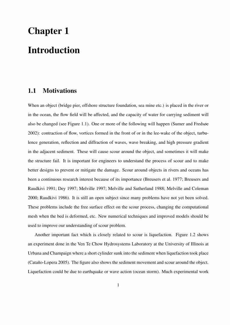
When an object (bridge pier, offshore structure foundation, sea mine etc.) is placed in the river or
in the ocean, the flow field will be affected, and the capacity of water for carrying sediment will
also be changed (see Figure 1.1). One or more of the following will happen (Sumer and Fredsøe
2002): contraction of flow, vortices formed in the front of or in the lee-wake of the object, turbu-
lence generation, reflection and diffraction of waves, wave breaking, and high pressure gradient
in the adjacent sediment. These will cause scour around the object, and sometimes it will make
the structure fail. It is important for engineers to understand the process of scour and to make
better designs to prevent or mitigate the damage. Scour around objects in rivers and oceans has
been a continuous research interest because of its importance (Breusers et al. 1977; Breusers and
Raudkivi 1991; Dey 1997; Melville 1997; Melville and Sutherland 1988; Melville and Coleman
2000; Raudkivi 1986). It is still an open subject since many problems have not yet been solved.
These problems include the free surface effect on the scour process, changing the computational
mesh when the bed is deformed, etc. New numerical techniques and improved models should be
used to improve our understanding of scour problem.
Another important fact which is closely related to scour is liquefaction. Figure 1.2 shows
an experiment done in the Ven Te Chow Hydrosystems Laboratory at the University of Illinois at
Urbana and Champaign where a short cylinder sunk into the sediment when liquefaction took place
(Catano-Lopera 2005). The figure also shows the sediment movement and scour around the object.
Liquefaction could be due to earthquake or wave action (ocean storm). Much experimental work
1

(a)
(b)
Figure 1.1: Scour around Piles: (a) Bridge Pier (www.ifh.uni-karlsruhe.de) (b) Scour Experimentin Hydrosystems Laboratory, University of Illinois
2
has been done (Sakai et al. 1994; Sumer et al. 1999), and numerical models have been developed
(Magda 1996; Jeng and Lin 1999; Gao et al. 2003) to understand this complicated process. There
are also many analytical models which describe the sea bed response and give fairly good results
(Yamamoto 1977; Mei and Foda 1981; Jeng and Hsu 1996; Yuhi and Ishida 2002). Although there
exists many numerical models on sea bed response under waves, most of them simply estimate
wave pressure distribution on the water-bed interface using wave theory. This is true if there are
only water waves and sea bed interactions. However, for the case when there are extra objects
in the system (such as pile, semi-buried foundation, etc.), the water flow around the object will
be highly three-dimensional, therefore making it difficult to get an analytical solution from wave
theory. With the use of computational fluid dynamics (CFD), the flow field can be solved and used
as an input for the numerical modeling of liquefaction.
Other mechanisms, as pointed out in Bennett and Dolan (2001), such as impact penetration,
gravity settlement, bedform migration, shakedown, sliding, even biological activity will also have
important effects on the interactions between object, fluid and sea bed. These mechanisms are not
completely understood (Catano-Lopera 2005). They are closely related and affect each other. The
whole process is governed by the joint action of all these mechanisms even though some of them
might be dominant. In this research, only scour and liquefaction will be investigated.
1.2 Objectives of This Research
The main goal of this research is to use numerical models to predict the effect of scour and lique-
faction around objects.
For the scour process, two-dimensional and three-dimensional models are developed respec-
tively to predict scour under different temporal and spatial scales. The 2D model will utilize the
Godunov scheme and approximate Riemann solvers. Other depth-averaged 2D numerical models
in the literature for sediment transport and river morphology have obtained good results with this
approach, for example Duan and Nanda (2006) and Wu (2004) among many others. These models
3
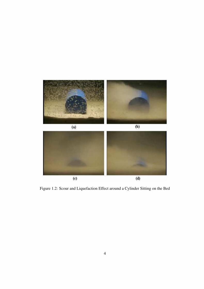
Figure 1.2: Scour and Liquefaction Effect around a Cylinder Sitting on the Bed
4

usually assume that the time scale of sediment transport is much larger than that of the flow field.
Based on this assumption, the quasi-steady approach is used most of the time. However, this as-
sumption is not always true when the bed morphological change is fast. In this thesis, a coupled
two-dimensional model for both hydrodynamics and sediment transport will be developed. Also,
the computational domain for a real world case is complicated, and an unstructured mesh is nec-
essary. Numerical calculation of the system wave speeds when using unstructured mesh is slow
and inefficient. Asymptotic expansion is used to estimate such wave speeds. The model developed
in this research can deal with wetting and drying automatically. Discontinuity of the flow can
be captured. In the 3D model, since there are at least three phases (water, object and sediment),
the interfaces between these phases need to be captured. Although different interface capturing
methods can be used, each interface has its own characteristics and appropriate methods should
be chosen for each of them. For the free water surface, an Eulerian approach is used while for
the bed interface, a Lagrangian approach is chosen. To take into account the deformation of the
fluid domain, a mesh deformation method should be used to smoothly move each grid point in the
domain.
For the liquefaction process, two different mechanisms (momentary and residual) will be con-
sidered. For momentary liquefaction, a three-dimensional numerical model for the sea bed re-
sponse under free surface water waves will be developed. Free surface is modeled by the volume
of fluid (VOF) method, and water waves are generated by numerical wave maker boundary con-
dition. An iterative numerical scheme is proposed to solve the Biot consolidation equation using
the finite volume method (FVM). The coupling between water wave and sea bed is through pres-
sure and stress condition on common boundaries. For residual liquefaction, the solutions to the
one-dimensional model equation of the period-averaged pore pressure buildup are listed. A source
term is added to the storage equation to model the pore pressure buildup. Corrections to the so-
lutions available in the literature are provided. For deep soil, an asymptotic solution is proposed
to estimate the pore pressure. In addition, a tentative step is made to model the phase-resolved
residual pore pressure.
5

The numerical models developed in this study can be used in engineering practice as a tool
to guide the design, construction, and operation of structures in rivers and oceans. These models
can also be used as a research tool to further understand the complete mechanisms of scour and
liquefaction.
1.3 Methodology
This study is mainly based on numerical models. For scour problem, two-dimensional and three-
dimensional numerical models are developed to simulate the flow field and sediment transport
processes. Both codes are based on the finite volume method. The two-dimensional code solves
the shallow water equations on unstructured meshes. It is suitable for large scale and long term
simulations. This is an in-house research code developed in the Ven Te Chow Hydrosystems
Laboratory at UIUC. The three-dimensional code is developed on the platform of an open source
computational fluid dynamics (CFD) code named OpenFOAM (OpenCFD 2006). The fluid flow
solver is adapted from the original turbulence flow solver and a sediment transport solver is added
to it. For liquefaction potential simulation, the numerical model is also based on OpenFOAM since
it provides a platform for the numerical solution of partial differential equations. Coupled solver
of free surface flow and consolidation is developed to simulate the sea bed response under waves.
Numerical test cases are selected from the literature for the purpose of validation and testing of the
capabilities of the model.
Most of the simulations are done in the supercomputers in National Center for Supercomputing
Applications (NCSA) at University of Illinois at Urbana and Champaign. Parallel computations
are used (especially the three dimensional model of scour and liquefaction) extensively to reduce
the required computer time.
6

1.4 Outline of the Dissertation
In chapter 2, the two-dimensional numerical model for scour is introduced. The finite volume
method solver for the non-linear shallow water equations is described. Two-dimensional Riemann
problem approximate solvers used in the code are briefly described. Numerical simulations of
scour problems in a large domain and for long evolution time are carried out. In Chapter 3, the
three-dimensional scour model with free water surface and automatic mesh deformation is elabo-
rated. Free surface capturing methods and bed surface resolving methods are described. A novel
mesh deformation method is used to automatically move the mesh for the scour problem. Dis-
cussions on the merits and shortcomings of different interface capturing methods are given at the
end of the chapter. Chapter 4 describes the three-dimensional, coupled model for the liquefaction
evaluation. Fluid field solver is similar to that of three-dimensional scour model while consolida-
tion solver is written based on the new iterative algorithm using finite volume method. Chapter
5 introduces the one-dimensional period-averaged residual pore water buildup model. Corrected
solutions and a new asymptotic estimation for deep sediment deposits are given. Numerical model
is also developed for the period-averaged pore pressure. A tentative step is made to model the
phase-resolved pore pressure numerically. Chapter 6 is a summary of the thesis findings. In the
appendixes, the derivations of some of the equations used in this thesis are given.
7
Chapter 2
Two Dimensional Model for Scour AroundObject Using Shallow Water Equations onUnstructured Mesh
2.1 Introduction
Scour due to sediment transport has been one of the most important engineering problems be-
cause it will endanger the stability of structures such as bridges (Sumer and Fredsøe 2002). Many
two-dimensional and three-dimensional numerical models have been developed to simulate the
scour process (Beek and Wind 1990; Olsen and Melaaen 1993; 1999; Brørs 1999; Li and Cheng
2001; Neyshabouri et al. 2003; Duc et al. 2004; Wu 2004; Roulund et al. 2005; Duan and Nanda
2006). While three-dimensional models can give more detailed information on the flow and tur-
bulence structure, they require considerable computational efforts (Liu and Garcıa 2006a). Two-
dimensional models can give quick assessment of the scour pattern and relatively accurate max-
imum scour depth. The fast evaluation of these scour parameters are important for the design,
construction and operation of hydraulic structures. It is of critical importance in the case of scour
due to dam failure or dike break flow. In this paper, a two-dimensional model coupling hydrody-
namic and scour processes will be developed.
The hydrodynamic component of many two-dimensional models is the depth averaged shal-
low water equations (SWEs) in which the hydrostatic assumption is implied. Higher order finite
volume methods on unstructured triangular grids for shallow water equations have been developed
and have achieved high accuracy (Anastasiou and Chan 1997; Yoon and Kang 2004). The unstruc-
∗This chapter, as a manuscript, is under review for possible publication in Coastal Engineering
8

tured mesh makes the application of SWEs for complex geometries easier. However, the treatment
of the pressure and bed-slope terms should be compatible with other terms in the equations when
discretizing on an unstructured mesh (Farshi and Komaei 2005). Special care should be taken to
make the scheme compatible and conservative. Otherwise, non-physical results will be observed
after several time steps (Nujic 1995).
For finite volume methods (FVM) solving shallow water equations, one of the most important
properties is called the C-property which describes the stationary state when the flux gradients
balance the slope source term (Bermudez and Vazquez 1994). LeVeque (1998) developed a wave-
propagation algorithm by solving the Riemann problem at the cell center and canceling the source
term with the flux difference exactly. Another important contribution in dealing with this problem
is the surface gradient method (SGM) (Zhou et al. 2001; 2002). The basic assumption is that the
water surface is smoother than the bottom. Instead of conservative variables, the surface gradi-
ent method uses the water surface level to reconstruct the Riemman states at the cell interfaces.
Rogers et al. (2003) proposed a novel method which reformulates the conservation laws in terms
of the deviations from equilibrium. This mathematical reformulation introduces extra physical
information and avoids the conventional numerical treatment of the imbalance. Another method
of equation reformulation is to rewrite the bed slope term in divergence form. An exact balance
between flux gradient and source term is achieved when both terms are discretized by compatible
schemes (Valiani and Begnudelli 2006; Liu and Garcıa 2007b). For the hyperbolic system which is
expanded by adding sediment transport equation in this chapter, the divergence form is not suitable
for the source term.
Godunov scheme with an appropriate Riemann solver can capture the steep water surface el-
evation gradient even discontinuities. For the coupled system of hydrodynamics and sediment
transport, it can be used where a dramatic water surface change occurs, e.g. scour due to dam
break flow and strong transient flow. Based on the hyperbolic nature of the coupled system, De-
Vriend (1987a) and DeVriend (1987b) analyzed the waves and their interactions, although the
analysis was on the system of primitive variables. Since then, the coupled system of shallow water
9
and bed sediment conservation equations has been studied by many researchers. Lyn (1987) and
Lyn and Altinakar (2002) identified the different scales of the one-dimensional system and gave the
asymptotic approximation of the wave speeds in different flow regimes. For one-dimensional sys-
tem under some simplifications, the wave speeds can be expressed explicitly (Hudson and Sweby
2003; Hudson et al. 2005). On a structured mesh, the waves associated with the two-dimensional
system can also be analyzed by splitting the system into different directions (Hudson and Sweby
2005). On a unstructured mesh, the equation system is more complicated and difficult to analyze.
This is one of the problems which will be dealt with in this paper.
There is still a debate on the characteristic of the coupled system of SWEs and sediment con-
servation equation (i.e., Exner’s equation). Cao et al. (2002) emphasized on the hyperbolicity of
the coupled system while Cui et al. (2005) argued that the evolution of the sediment waves can be
dominated by dispersion. Different interpretation of the equations is most often due to the differ-
ent flow regimes. In different regimes, the dominant terms in the governing equations will change.
Cui and Parker (1997) did some linear stability analysis and found the conditions for the dispersive
domination are that the Froude number should not be too far from unity, the sediment transport
rate should be low, and the wavelength of the bed forms should be long. In the author’s opinion,
the question of which term is dominant is only relevant for analysis. Since for a numerical model
all the terms are included, the nature of the coupled system will reveal itself through the simulation
results.
In this chapter, the hydrodynamics and sediment transport are coupled and solved together in
one step. Special treatment of the source term on unstructured grid will make the scheme stable
and physically balanced (conserving both mass and momentum). The methodology of expanding
the SWEs with sediment transport can also be used to expand the system with other equations
(such as scalar transportation). Asymptotic analysis of the system eigenvalues will be given and
the approximation will be compared with the numerical results. Finally, test cases will be used to
verify the numerical model. The hydrodynamic part of the model is tested against the experiment
of dam break flow in an 90 bend. Then, the coupled model is tested on the scour problem around a
10

spur dike by surge waves. The result from the coupled model will be compared with the traditional
model with a quasi-steady approach.
2.2 Governing Equations
2.2.1 Shallow Water Equations
The governing equations are the non-linear shallow water equations
∂ξ
∂t+
∂(uh)
∂x+
∂(vh)
∂y= 0 (2.1)
∂(uh)
∂t+
∂(u2h)
∂x+
∂(uvh)
∂y− ν
(∂(hux)
∂x+
∂(huy)
∂y
)=
τwx − τbx
ρ− gh
∂ξ
∂x+ hfv (2.2)
∂(vh)
∂t+
∂(uvh)
∂x+
∂(v2h)
∂y− ν
(∂(hvx)
∂x+
∂(hvy)
∂y
)=
τwy − τby
ρ− gh
∂ξ
∂y− hfu (2.3)
where ξ is the free surface elevation above the still water level hs, h is the total water depth
(= hs + ξ), u and v are the depth-averaged velocities in the x and y directions respectively, t is
time, τwx and τwy are wind shear stresses, τbx and τby are bottom friction forces, ν is the viscosity,
g is the gravity constant, and f is the Coriolis parameter.
In order to obtain the hyperbolic formulation, the gh ∂ξ∂x
and gh ∂ξ∂y
terms are split according to
gh∂ξ
∂x=
1
2g∂(ξ2 + 2ξhs)
∂x+ gξSox (2.4)
gh∂ξ
∂y=
1
2g∂(ξ2 + 2ξhs)
∂y+ gξSoy (2.5)
Using this splitting approach, the shallow water equations (Eqns. 2.1,2.2,2.3) can be rewritten
as∂ξ
∂t+
∂(uh)
∂x+
∂(vh)
∂y= 0 (2.6)
11

∂(uh)
∂t+
∂(u2h + 12g(ξ2 + 2ξhs))
∂x+
∂(uvh)
∂y− ν
(∂(hux)
∂x+
∂(huy)
∂y
)
=τwx − τbx
ρ− gξSox + hfv
(2.7)
∂(vh)
∂t+
∂(uvh)
∂x+
∂(v2h + 12g(ξ2 + 2ξhs))
∂y− ν
(∂(hvx)
∂x+
∂(hvy)
∂y
)
=τwy − τby
ρ− gξSoy − hfv
(2.8)
2.2.2 Sediment Conservation and Transport Equations
Only bed load is considered in this work. There are many bed load transport rate formulas in the
literature in which most of them relate bed load transport rate with bed shear stress. However,
an alternative simple formula, the Grass formula (Grass 1981), which relates the bed load to flow
velocities is often used in many sediment transport numerical models (Cao et al. 2002; Hudson
and Sweby 2003; Hudson et al. 2005). The Grass formula has the form
qsx = Au(u2 + v2
)m−12 (2.9)
qsy = Av(u2 + v2
)m−12 (2.10)
where A and m are parameters determined by the properties of the sediment. In this paper, A =
0.001 and m = 3 are chosen which correspond to fine sand. qsx and qsy are the sediment transport
rate in the x and y directions respectively.
The conservation law of the sediment is described by the Exner equation (Garcıa 1999)
∂z
∂t+
1
1− ε0
(∂qsx
∂x+
∂qsy
∂y
)= 0 (2.11)
where z is the bed elevation, ε0 is the sediment porosity.
12

2.3 Numerical Method of the Model
Integrating the governing equations over the domain Ω and using Green’s theorem, the integral
form of the governing equation can be written asW nSFigure 2.1: Scheme of the Computational Domain
∂
∂t
∫∫
Ω
Q dΩ +
∮
S
F · ndS =
∫∫
Ω
HdΩ (2.12)
where Ω is the domain of interest, S is the boundary of Ω (see Figure. 2.1), n is the outward
surface normal vector of S, Q is the conservative variables vector, F is the flux vector, and H is
the source term vector. The forms of Q, F, and H will be listed in the following sections. F can
be split into viscous and inviscid flux components as follows:
F · n = F I − F V =(f I − νfV
)nx +
(gI − νgV
)ny (2.13)
where nx and ny are the Cartesian components of the normal vector (√
n2x + n2
y = |n|=1), and
superscripts I and V denote invicid and viscous components respectively.
13

2.3.1 Quasi-Steady Approach
For quasi-steady approach, the SWEs are analyzed separately from the Exner equation. Just for
the SWEs, Q, F and H have the forms
Q =
ξ
uh
vh
f I =
uh
u2h + g(ξ2 + 2ξhs)/2
uvh
gI =
vh
uvh
v2h + g(ξ2 + 2ξhs)/2
fV =
0
h∂u∂x
h ∂v∂x
gV =
0
h∂u∂y
h∂v∂y
H =
0
τwx−τbx
ρ− gξSox + hfv
τwy−τby
ρ− gξSoy − hfu
(2.14)
The Exner equation is also descretized using the FVM and Green theorem as Eqn. 2.12. How-
ever, the Godunov scheme is not used here simply because the sediment transport rate is not a
function of the bed elevation z and therefore the Jacobian matrix (only one element in this case)
can not be evaluated. The fluxes across the cell interfaces are calculated using the variable values
at the edges. For the Exner equation, Q, F, and H have the forms
Q = z F · n =1
1− ε0
(qsxnx + qsyny) H = 0.
14

2.3.2 Coupled Approach
For the coupled approach, the SWEs and Exner equation form an expanded system. Q, F, and H
have the forms
Q =
ξ
uh
vh
z
f I =
uh
u2h + g(ξ2 + 2ξhs)/2
uvh
11−ε0
qsx
gI =
vh
uvh
v2h + g(ξ2 + 2ξhs)/2
11−ε0
qsy
fV =
0
h∂u∂x
h ∂v∂x
0
gV =
0
h∂u∂y
h∂v∂y
0
H =
0
τwx−τbx
ρ− gξSox + hfv
τwy−τby
ρ− gξSoy − hfu
0
(2.15)
2.4 Evaluation of Numerical Fluxes
The fluxes F across the interface between each two triangles are separated into inviscid and viscous
fluxes. The numerical treatment of these two fluxes are different. For the inviscid fluxes, the one-
dimensional Riemann problem is extended to two dimensions. Analytical or approximate solvers
of the Riemann problem can be used to evaluate the fluxes. While for the viscous fluxes, the
evaluation of the velocity gradient is taken at the edge’s center which can be used to calculate the
viscous fluxes.
2.4.1 Inviscid Fluxes
The analytical solver of Riemann problem is slow comparing with the approximate solvers. Among
many choices of approximate solvers, Roe’s approach (Roe 1981; 1986) is used in this work. The
15

inter-cell inviscid flux FIi,j by Roe’s solver can be written as
FIi,j =
1
2
[FI(Q+
i,j) + FI(Q−i,j)− |A| (Q+
i,j −Q−i,j)
](2.16)
|A| = R |Λ|L (2.17)
where Q+i,j and Q+
i,j are reconstructed Riemann state variables on the right and left sides, respec-
tively. A is the flux Jacobian matrix defined by
A =∂F · n∂Q
(2.18)
Quasi-Steady Approach
Since the uncoupled approach will be compared with the coupled approach, the flux Jacobian of
the two-dimensional SWEs system without the Exner equation takes the form:
A =∂F · n∂Q
=
0 nx ny
(c2 − u2)nx − uvny 2unx + vny uny
−uvnx + (c2 − v2)ny vnx unx + 2vny
(2.19)
The three distinct eigenvalues of A (by hyperbolicity of the system) are
λ(1) = unx + vny, λ(2) = unx + vny − c, λ(3) = unx + vny + c (2.20)
while the left and right eigenvector matrices are
R =
0 1 1
ny u− cnx u + cnx
−nx v − cny v + cny
(2.21)
16
nL Ri j=1j=3 j=2nnFigure 2.2: Control Volume Scheme
L =
−(uny − vnx) ny −nx
unx+vny
2c+ 1
2−nx
2c
−ny
2c
−unx+vny
2c+ 1
2nx
2c
ny
2c
(2.22)
The Riemann state variables u, v, and c on the face boundaries which are needed to calculate
the flux are given by Roe’s average as
u =u+√
h+ + u−√
h−√h+ +
√h−
, v =v+√
h+ + v−√
h−√h+ +
√h−
, c =
√g(h+ + h−)
2(2.23)
and the superscripts + and − refer to the right and left side of the edge.
17

Coupled Approach
The coupled approach needs further reformulation of the H vector in Eqn. 2.15. The slope term
in H is split and written in matrix form as
H =
0
τwx−τbx
ρ− gξSox + hfv
τwy−τby
ρ− gξSoy − hfu
=
0
τwx−τbx
ρ+ ghsSox + hfv
τwy−τby
ρ+ ghsSoy − hfu
︸ ︷︷ ︸(1)
+
0
−ghSox
−ghSoy
︸ ︷︷ ︸(2)
(2.24)
Term (2) in Eqn. 2.24 will be moved to the left hand side of the governing equation and combined
with the Jacobian matrix of the SWEs fluxes. The purpose of this reformulation is to get a non-
singular Jacobian matrix. This approach is also used in Hudson and Sweby (2003) and Hudson
et al. (2005). But their governing shallow water equations are in different forms from those in this
research.
The invicid fluxes on the unstructured mesh for the coupled approach can not be expressed
explicitly as for the quasi-steady approach since the 4× 4 Jacobian matrix is far more complicated
than the 3× 3 Jacobian matrix of the quasi-steady approach. In this paper, an asymptotic analysis,
instead of an analytical expression, is used to approximate the eigenvalues of the Jacobian matrix
of the coupled approach. This is shown in the next section.
2.5 Asymptotic Analysis of the Wave Speeds
In order to give the asymptotic analysis of the two-dimensional system, it is necessary to consider
the approximation for the one-dimensional system since they are closely related to each other.
18

2.5.1 One-Dimensional System
The analysis for one-dimensional system is similar to Lyn (1987) and Lyn and Altinakar (2002).
The general procedure of solving an algebraic equation using asymptotic approximation can be
found in Nayfeh (1981). The Jacobian matrix for one-dimensional system has the form
J1D =∂F(Q)
∂Q=
0 1 0
−u2 + gh 2u gh
−k u3
hk u2
h0
(2.25)
where k = 3A/ (1− ε0) > 0. The eigenvalues are the roots of the equation
λ3 − 2uλ2 + λ(u2 − gh− kgu2
)+ kgu2 = 0 (2.26)
where k 7→ 0+. Eqn. 2.26 has three distinct roots because the discriminant
∆ = −g[4hu4 + 4g2
(h + ku2
)3+ g
(−8h2u2 + 20hku4 + k2u6)]
= −g[4hu4 + 4g2h3 − 8gh2u2 +
(12g2h2u2 + 20ghu4
)k + O(k2)
]
= −g
4g2h3
(Fr2 − 1
)2
︸ ︷︷ ︸≥0
+(12g2h2u2 + 20ghu4
)k︸ ︷︷ ︸
>0
+O(k2)
< 0
where Fr = u/(gh). Let ε = kg and λ = λ/u, then the characteristic Eqn. 2.26 becomes
λ3 − 2λ2 + λ
(1− 1
Fr2− ε
)+ ε = 0 (2.27)
The results are listed here and the details of the asymptotic analysis are in Appendix A. Since
the regular expansion is not uniform when the flow is near critical, a change of scale is used to
achieve an uniform expansion. When the flow is far away from critical state, i.e. 1− 1/Fr2 À 0,
19

the three eigenvalues are given by
λ(1) =ε
1Fr2 − 1
(2.28)
λ(2) = 1 +1
Fr+
ε
2(
1Fr
+ 1) (2.29)
λ(3) = 1− 1
Fr− ε
2(
1Fr− 1
) (2.30)
When the flow is near critical, i.e.(1− 1
Fr2
) ∼(ε
12
), the three eigenvalues are
λ(1) =2
3+
1
2Fr2(2.31)
λ(2) =1
4
1− 1
Fr2+
√(1− 1
Fr2
)2
+ 8ε
(2.32)
λ(3) =1
4
1− 1
Fr2−
√(1− 1
Fr2
)2
+ 8ε
(2.33)
2.5.2 Two-Dimensional System
For a two-dimensional system, the Jacobian matrix is
J2D =∂F (Q) · n
∂Q= Anx + Bny (2.34)
where
A =
0 1 0 0
−u2 + gh 2u 0 gh
−uv v u 0
−3ku(u2+v2)
hk(3u2+v2)
h2k uv
h0
(2.35)
20

and
B =
0 0 1 0
−uv v u 0
−v2 + gh 0 2v gh
−3kv(u2+v2)
h2k uv
hk(u2+3v2)
h0
(2.36)
Direct calculation of the eigenvalues/vectors of matrix J2D, which is in the original global x−y
coordinate system, is difficult. In this work, the calculation of the Roe’s fluxes is done in a local
ξ − η coordinates of each cell-to-cell interface where one of the coordinates coincides with the
outward normal vector (see Fig. 2.3). This will simplify the calculation. The following theorem
gives the relationship between the fluxes in the global and local coordinate systems.
x
y
i
_ +n
j=1
j=2
j=3
Figure 2.3: Local Coordinate at the Cell Interface
Theorem 2.5.1. In the global and local coordinates shown as in Fig. 2.3, for the two-dimensional
coupled system, suppose the interfacial Roe’s flux defined in Eq. 2.16 are Fij,g and Fij,l respec-
tively, where each flux is a vector with 4 components. Also define the transformation matrix M
as
M =
cos(θ) sin(θ)
− sin(θ) cos(θ)
(2.37)
21

Define sub-vectors Fsub,g = [Fij,g(2) Fij,g(3)]T and Fsub,l = [Fij,l(2) Fij,l(3)]T . Then
1. Fij,g(1) = Fij,l(1) and Fij,g(4) = Fij,l(4)
2. Fsub,g = M · Fsub,l
Proof. The mass fluxes of water and sediment are invariant of the coordinate rotation. This means
the water and sediment across the cell interface will not change under different coordinate ref-
erences. The first and fourth components of the flux vector are the mass fluxes for water and
sediment respectively. Then, the components can be written as
Fij,g(1) = Fij,l(1) and Fij,g(4) = Fij,l(4)
For the momentum fluxes of water (the second and third components of the flux vector), they
follow the rule of rotational transformation stated below since they are two-dimensional vectors in
the plane.
Fsub,g = M · Fsub,l
The alternative approach of the proof is to use the Jacobian matrixes in the global and local co-
ordinates and calculate the eigenvalues/vectores respectively. Calculation of the Roe’s flux vector
in the two coordinate systems will verify the conclusion of the theorem. However, the difficulty of
this proof strategy is the calculation of the eigenvalues/vectors of the global Jacobian matrix. From
the authors’ experience, it is hard to find an explicit expression of eigen-system for the global Jaco-
bian. Even with some simplifications, the explicit expression is lengthy and not practically useful.
Thus, this complication motivates the use of the coordinate transformation so that the fluxes can
be evaluated in the local coordinates which is simple and easy to analyze.
In the local coordinate, since nξ = 1 and nη = 0 (where nξ and nη are the outward normal
vector component in ξ and η directions), the Jacobian matrix in terms of the transformed velocity
22

vectors has the form of
J2D,l =
0 1 0 0
−u2ξ + gh 2uξ 0 gh
−uξvη vη uξ 0
−3kuξ(u2
ξ+v2η)
hk(3u2
ξ+v2η)
h2k
uξvη
h0
(2.38)
This Jacobian matrix is similar to that in Hudson and Sweby (2005) in which their analysis is
for structured mesh. One of the eigenvalues of J2D,l is uξ, while the other threes are the solution
of the polynomial equation
λ3 − 2uξλ2 + λ
[u2
ξ − gh− kg(3u2
ξ + v2η
)]+ kguξ
[3u2
ξ + v2η
]= 0 (2.39)
Eqn. 2.39 has three distinct roots because the discriminant is negative.
∆ = g[−4hu4
ξ − 4g2(h + k
(3u2
ξ + v2η
))− gu2ξ
(−8h2 + 20hk(3u2
ξ + v2η
)+ k2
(3u2
ξ + v2η
))]
= −g[4hu4
ξ − 8gh2u2ξ + 4g2h3 + gh
(12gh + 20u2
ξ
) (3u2
ξ + v2η
)k + O(k2)
]
= −g
4h
(u2
ξ − gh)2
︸ ︷︷ ︸≥0
+ gh(12gh + 20u2
ξ
) (3u2
ξ + v2η
)k︸ ︷︷ ︸
>0
+O(k2)
< 0
If uξ = 0, the three roots of Eqn. 2.39 are 0,√
gh + kgv2η , and −√
gh + kgv2η . The eigen-
systems for the cases of uξ = 0 are list in Appendix A.2. For the general case of uξ 6= 0, defining
ε = kg(3u2
ξ + v2η
)/u2
ξ and λ = λ/uξ, Eqn. 2.39 can be written as
λ3 − 2λ2 + λ
[1− 1
Fr2− ε
]+ ε = 0
where Fr = uξ/gh. This is the same as the form for one-dimensional case and the eigenvalues can
be approximated using perturbation analysis as in Eqns. 2.28 to 2.31. In summary, the eigenvalues
23

λi and right eigenvectors Ri for the two-dimensional system in the local coordinate are listed
below. The right eigenvector matrix is
R =
−2kvη −gh −gh −gh
−2kuξvη −ghλ(2) −ghλ(3) −ghλ(4)
h− 2kv2η −ghvη −ghvη −ghvη
2kvη gh−(λ(2) − uξ
)2
gh−(λ(3) − uξ
)2
gh−(λ(4) − uξ
)2
(2.40)
and the left eigenvector matrix is
L =
−vη
h0 1
h0
a1−a2λ(4)−λ(3)(a2+a3λ(4))gh2b1
−2uξ+λ(3)+λ(4)
ghb1
−2kvη(uξ−λ(3))(uξ−λ(4))gh2b1
−1b1
a1−a2λ(4)−λ(2)(a2+a3λ(4))gh2b2
−2uξ+λ(2)+λ(4)
ghb2
−2kvη(uξ−λ(2))(uξ−λ(4))gh2b2
−1b2
a1−a2λ(3)−λ(2)(a2+a3λ(3))gh2b3
−2uξ+λ(2)+λ(3)
ghb3
−2kvη(uξ−λ(2))(uξ−λ(3))gh2b3
−1b3
(2.41)
where a1 = −gh2+hu2ξ+2ku2
ξv2η; a2 = 2kuξv
2η , a3 =
(h− 2kv2
η
); b1 =
(λ(2) − λ(3)
)(λ(2) − λ(4)
);
b2 =(λ(3) − λ(2)
)(λ(3) − λ(4)
); and b3 =
(λ(4) − λ(2)
)(λ(4) − λ(3)
).
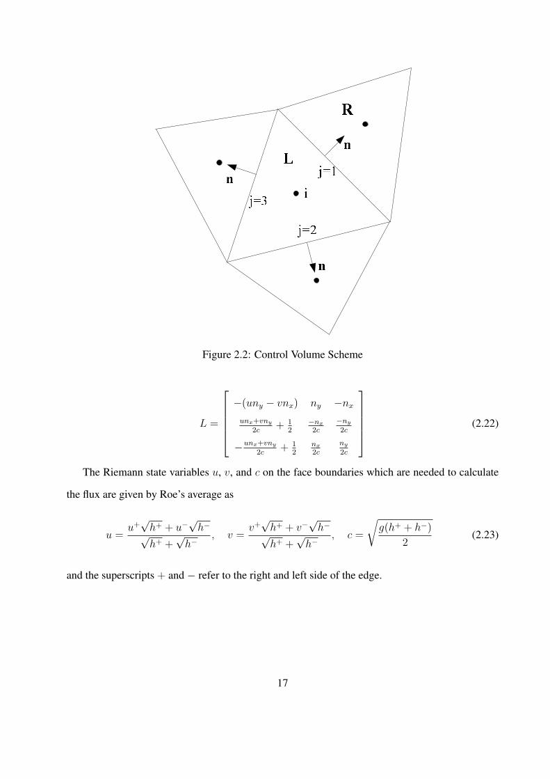
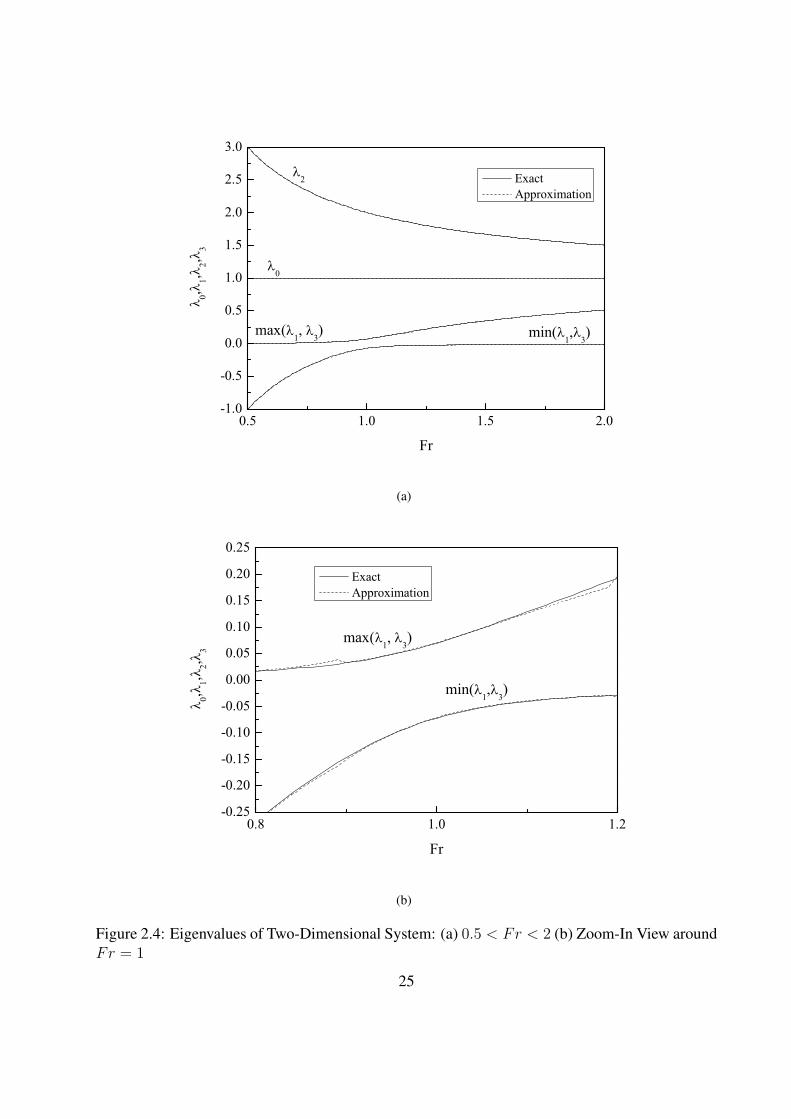
The eigenvalues of the two-dimensional system can also be calculated using a numerical
method. For comparison, the four eigenvalues from both the asymptotic approximation and the
numerical method are plotted in Fig. 2.4 with ε equal to 0.01. The figures are similar to those in
Lyn and Altinakar (2002). Fig. 2.4(a) shows the four eigenvalues for Fr between 0.2 and 2. For
Fr > 1.2 or Fr < 0.8, the regular expansion formula is used, while for 0.8 < Fr < 1.2, the
re-scaled expansion formula is used. Both asymptotic approximation and numerical results are
shown in the figure. Results from both methods are nearly identical. Major part of the error occurs
when the flow is near critical. where the relative error is within 1%.
24
0.5 1.0 1.5 2.0-1.0
-0.5
0.0
0.5
1.0
1.5
2.0
2.5
3.0
min(1,
3)max(
1,
3)
2
0,1,
2,3
Fr
Exact Approximation
0
(a)
0.8 1.0 1.2-0.25
-0.20
-0.15
-0.10
-0.05
0.00
0.05
0.10
0.15
0.20
0.25
min(1,
3)
max(1,
3)
0,1,
2,3
Fr
Exact Approximation
(b)
Figure 2.4: Eigenvalues of Two-Dimensional System: (a) 0.5 < Fr < 2 (b) Zoom-In View aroundFr = 1
25

2.5.3 Viscous Fluxes
Viscous fluxes are not evaluated via Roe’s flux function. Instead, the viscous fluxes are calculated
directly using the velocity gradient at the boundary. By Gauss’s theorem, the velocity gradient term
in the cell center can be estimated by closed line integral over the boundary of that cell (Anastasiou
and Chan 1997).
2.6 Limiter for High Order Schemes
The evaluation of the Riemann states on both sides of the cell interface needs interpolation since
all the conservative variables are stored at the cell center. This step is usually called variable
reconstruction. The following equation is the relation between the interpolated variable at an
arbitrary location (x, y) and the value at the cell center
Q(x, y) = Qc +∇Q · r (2.42)
where Qc is the variable value at cell center, ∇Q is the gradient of Q, and r is the vector from cell
center to (x, y). This is a piecewise linear interpolation which has second order accuracy. Second
and higher order schemes will introduce numerical oscillations. In order to maintain monotonicity,
non-linear limiters are introduced to eliminate oscillations in high gradient areas while keeping
high accuracy in smooth areas. The limited version of the reconstruction equation has the form
Q(x, y) = Qc + Φ(rf )∇Q · r (2.43)
where Φ is a function of rf , which is the upwind ratio of consecutive gradients of the variable. For
the structured mesh, rf is easy to calculate because the topological relation of upwind and down-
wind is clear. For the unstructured mesh, it becomes difficult. The so-called exact r formulation
in Darwish and Moukalled (2003) is used in this work. Fig. 2.5 shows the layout of the cells. For
26

face f , C and D are defined as the upwind and downwind cells according to the direction of the
flow velocity. U is defined as the virtual upwind cell of C. The formulation of rf is
rf =(2∇Qc · rCD)
QD −QC
− 1 (2.44)
where rCD is the vector connecting node C and D. After the ratio rf is calculated, it can be used
C
D
U
f
x
y
Figure 2.5: Exact r Formulation of the Limiter Function
in the limiter functions. In this paper, the MINMOD Total Variation Diminishing (TVD) scheme
is used which has the following form
Φ(rf ) = max(0, min(1, rf )) (2.45)
27

2.7 Time Integration
The time integration used in the paper is similar to the method proposed by Anastasiou and Chan
(1997).∂(V Q)
∂t
∣∣∣∣n+1
i
= −∮
Si
Fni · ndS + V n
i Hni (2.46)
Qn+1i = Qn
i +∆t
V ni
(α
∂(V Q)
∂t
∣∣∣∣n+1
i
+ (1− α)∂(V Q)
∂t
∣∣∣∣n
i
)(2.47)
when α = 0, it becomes the Euler explicit scheme, while α = 1 results in a first order Euler
implicit method. For the explicit scheme, the time step is restricted by the Courant-Friedrichs-
Lewy (CFL) condition. As in Yoon and Kang (2004), the following formula is used to determine
the maximum time step allowed
∆t ≤ min(
Ri
2maxj(√
u2 + v2 + c)ij
)(2.48)
where Ri is the distance between the centroids of triangle i and j. The minimum is taken for all
the triangles in the computational domain while the maximum is take for the three neighboring
triangles of triangle i.
2.8 Boundary Conditions
Boundary conditions are applied to the cell faces on the domain boundary. For the hydrodynamic
part of the model, the boundary conditions are the same as in Anastasiou and Chan (1997) and
Rogers et al. (2001). Those boundary conditions are briefly listed below. Sediment conditions on
the boundary are also discussed.
28
2.8.1 Walls
No-slip condition is applied to walls, i.e., (u, v) = (0, 0). For sediment transport, the flux through
the wall is also set to be zero which means no sediment particle will go through the solid boundary.
2.8.2 Open Boundaries
Conditions for the open boundaries, including inlet and outlet, are specified using the Riemann
invariants
(u, v)I · n + 2√
ghI = (u, v)B · n + 2√
ghB (2.49)
where subscripts I and B refer to the interface and the boundary, respectively.
For subcritical flow, if water depth hB is specified, then
(u, v)B · n = 2√
ghB(u, v)I · n + 2√
ghI − 2√
ghB (2.50)
and if velocity is specified, then
hB =
[(u, v)I · n + 2
√ghI − (u, v)B · n
]2
4g(2.51)
Sometimes, the water discharge qw = hB [(u, v)B · n] is specified. For this case, Eqn. 2.49 can be
rewritten as
(u, v)I · n + 2√
ghI =qw
hB
+ 2√
ghB (2.52)
A numerical method can be used to solve hB and then (u, v)B · n = qw
hB.
For the supercritical inlet, both the velocity vector and water depth should be specified. For the
supercritical outlet, no boundary condition is needed to specify and the velocity vector and water
depth on the boundary is the same as those in the adjacent interior.
For the sediment transport rate, the sediment flux on the inlet is specified as the sediment feed
rate. On the outlet, the sediment flux is set as having a zero gradient.
29

2.9 Test Problems
In this section, the proposed numerical model is tested. The first test problem is just for the
hydrodynamics where the bed is kept fixed. This is used to test the model capability to capture
shocks as well as the robustness of the model for complicated flow conditions. The second test
problem is for both the hydrodynamics and sediment transport. The flume bed is not fixed and a
scour hole develops due to the flow. Both coupled and uncoupled approaches are used to simulate
the process and the results are compared.
2.9.1 Dam Break Flow in Channels with 90 Bend
In this section, the hydrodynamics part of the model is tested against experimental observations.
Sharp bends appear in rivers very frequently and the effects of these bends on catastrophic flooding
waves are extremely important. Experiments for dam-break flood in a channels with a 90 bend
were done in the laboratory of the Civil Engineering Department of the University Catholique
de Louvain, Belgium. The details of the experiment can be found in S.Soares-Frazao and Zech
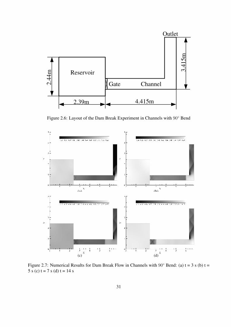
(2002). The layout of the experiment is shown in Fig. 2.6. The channel bed is 0.33 m above the
reservoir bed. The initial water surface level in the reservoir is 0.25 m above the channel bottom
while the channel bed is initially dry. The dam-break flood wave is generated by a sudden release
of the control gate. S.Soares-Frazao and Zech (2002) also developed a two-dimensional numerical
model to capture the flood wave. Good agreement of results between the experiment and numerical
model has been reported.
One of the most important factors which affect the extent of damage by dam-break floods is the
shock front and free water surface. In Fig. 2.7, the modeled free water surface elevation contours
at time t = 3 s, 5 s, 7 s, and 14 s are plotted. At t = 3 s, the flood wave has just reached the bend
which agrees with the experiment. The bend has at least two effects on the flood wave. One is
the reflection traveling upstream to the reservoir. The other effect is the reflection wave on the
downstream portion of the channel which can be seen in Fig. 2.7(d).
30
Reservoir
ChannelGate
Outlet
2.39m 4.415m
2.4
4m
3.4
15
m
Figure 2.6: Layout of the Dam Break Experiment in Channels with 90 Bend
(a) (b)
(c) (d)
Figure 2.7: Numerical Results for Dam Break Flow in Channels with 90 Bend: (a) t = 3 s (b) t =5 s (c) t = 7 s (d) t = 14 s
31

The modeled profiles of the water surface around the bend at different times are plotted in Fig.
2.8. The numerical results from S.Soares-Frazao and Zech (2002) are also plotted. The results
from both numerical models agree well with the experiment. From this figure, it is clear that
the upstream traveling reflection bore reaches the reservoir at around t = 14 s and after that the
water level recedes. The results from this test case show the capability of the model to capture the
complicated flow process and it is the basis of the coupled model simulation.
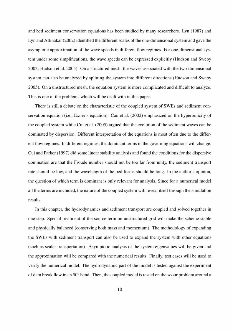
2.9.2 Scour Around the Spur Dike During a Surge Pass
The test case for the coupled model is the scour around a spur dike experiment from Mioduszewski
and Maeno (2003). The experiment was done in a laboratory flume at Okayama University, Japan.
Fig. 2.9(a) shows the plane view of the flume. The flume is 15 m long, 0.6 m wide, and 0.4 m deep.
The sand has d50 = 1.28 mm. The spur dike is not submerged. It is 6 cm thick and 15 cm wide.
Case 1 of the experiment is chosen for comparison. The water discharge was set to the value of Q
= 0.005 m3/s. The initial water depth is 20 cm and a surge wave is generated by opening the gate
at the downstream end of the flume at t = 0 s. The unstructured mesh for this test case is shown
in Fig. 2.9(b). The mesh around the spur dike is refined in order to capture the scour details. The
experiment also investigated the pore pressure in the sand due the pass of the surge wave. This
is also very important since the flow field and pressure distribution inside the sand will affect the
stability of the dike structure and scour process around it (Liu and Garcıa 2007a). However, the
pore pressure in the sand is beyond the scope of this paper and therefore it is not considered.
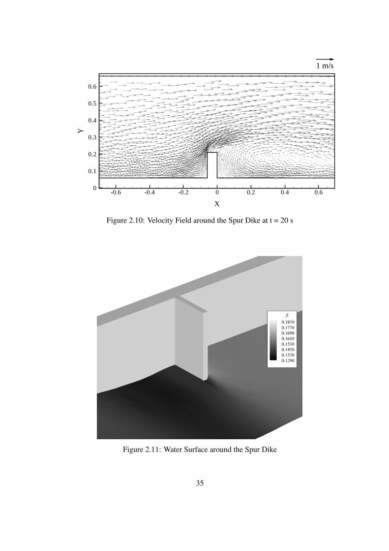
The velocity field around the spur dike at t = 20 s is plotted in Fig. 2.10. A recirculation zone
is formed behind the spur dike. Also because of the blocking effect of the dike, the flow velocity
is higher around the tip area. These flow characteristics are the cause of the sediment movement
and will affect the scour pattern. The free water surface around the spur dike at t = 20 s is plotted
in Fig. 2.11. Water elevation is higher in front of the spur dike and lower behind it.
In Fig. 2.12, the final scour patterns from the experiments, the quasi-steady simulation, and
the coupled approach simulation are shown. The basic scour pattern from the experiment is that
32

0.00
0.05
0.10
0.15
0.20
0.25
2 3 4 5 6 7 8 9
S (m)
z (m
)
Experiment
Soares-Frazão and Zech (2002)
Present Model
(a)
0.00
0.05
0.10
0.15
0.20
0.25
2 3 4 5 6 7 8 9
S (m)z
(m)
Experiment
Soares-Frazão and Zech (2002)
Present Model
(b)
0.00
0.05
0.10
0.15
0.20
0.25
2 3 4 5 6 7 8 9
S (m)
z (m
)
Experiment
Soares-Frazão and Zech (2002)
Present Model
(c)
0.00
0.05
0.10
0.15
0.20
0.25
2 3 4 5 6 7 8 9
S (m)
z (m
)
Experiment
Soares-Frazão and Zech (2002)
Present Model
(d)
Figure 2.8: Numerical Results for the Free Surface Profiles in Channels with 90 Bend: (a) t = 3 s(b) t = 5 s (c) t = 7 s (d) t = 14 s
33

Flow
0.6m
0.5m 0.5m
0.15m
0.06m
Sand Pit
(a)
X
Y
-0.6 -0.4 -0.2 0 0.2 0.4 0.60
0.1
0.2
0.3
0.4
0.5
0.6
(b)
Figure 2.9: Scour around the Spur Dike During a Surge Pass Experiment: (a) Experiment Layout(b) Unstructured Mesh around the Spur Dike
34
X
Y
-0.6 -0.4 -0.2 0 0.2 0.4 0.60
0.1
0.2
0.3
0.4
0.5
0.6
1 m/s
Figure 2.10: Velocity Field around the Spur Dike at t = 20 s
Figure 2.11: Water Surface around the Spur Dike
35
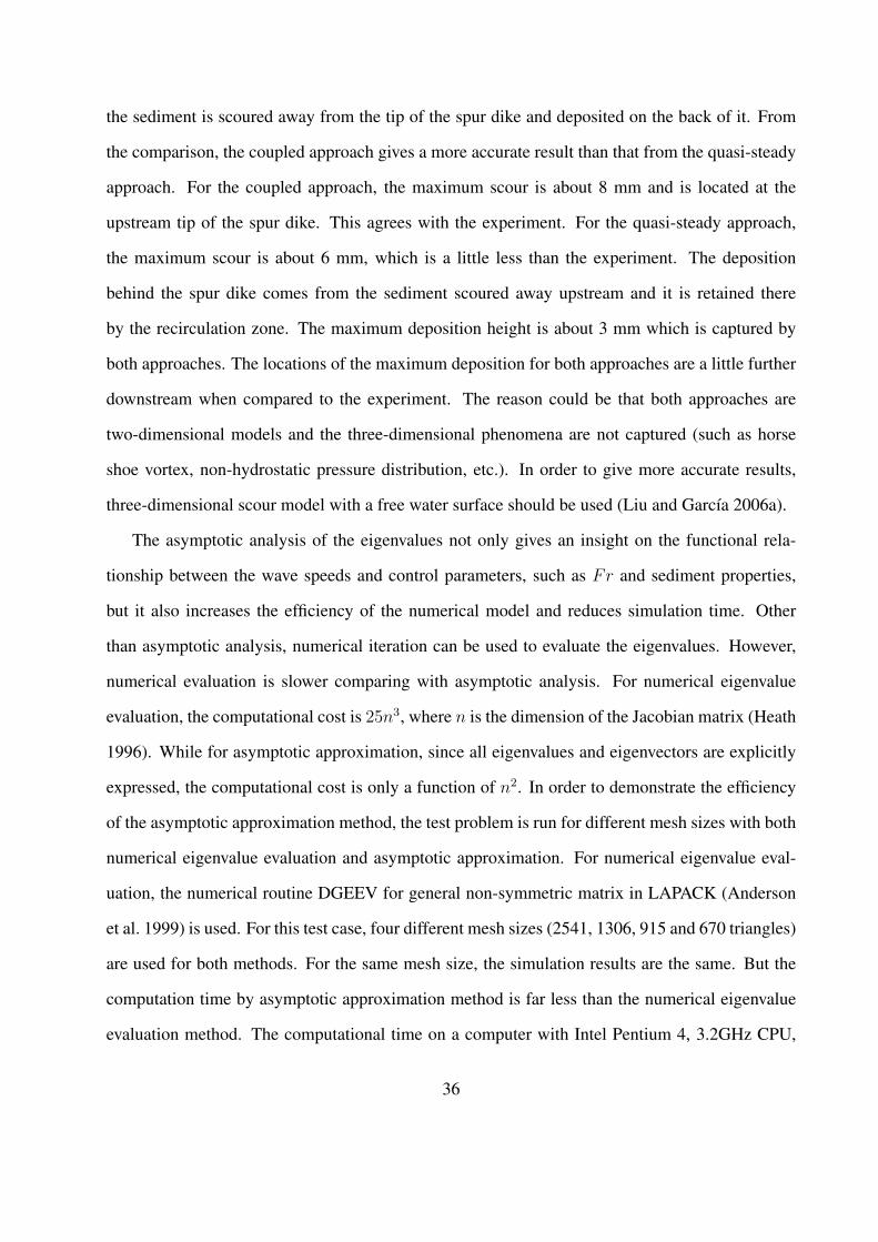
the sediment is scoured away from the tip of the spur dike and deposited on the back of it. From
the comparison, the coupled approach gives a more accurate result than that from the quasi-steady
approach. For the coupled approach, the maximum scour is about 8 mm and is located at the
upstream tip of the spur dike. This agrees with the experiment. For the quasi-steady approach,
the maximum scour is about 6 mm, which is a little less than the experiment. The deposition
behind the spur dike comes from the sediment scoured away upstream and it is retained there
by the recirculation zone. The maximum deposition height is about 3 mm which is captured by
both approaches. The locations of the maximum deposition for both approaches are a little further
downstream when compared to the experiment. The reason could be that both approaches are
two-dimensional models and the three-dimensional phenomena are not captured (such as horse
shoe vortex, non-hydrostatic pressure distribution, etc.). In order to give more accurate results,
three-dimensional scour model with a free water surface should be used (Liu and Garcıa 2006a).
The asymptotic analysis of the eigenvalues not only gives an insight on the functional rela-
tionship between the wave speeds and control parameters, such as Fr and sediment properties,
but it also increases the efficiency of the numerical model and reduces simulation time. Other
than asymptotic analysis, numerical iteration can be used to evaluate the eigenvalues. However,
numerical evaluation is slower comparing with asymptotic analysis. For numerical eigenvalue
evaluation, the computational cost is 25n3, where n is the dimension of the Jacobian matrix (Heath
1996). While for asymptotic approximation, since all eigenvalues and eigenvectors are explicitly
expressed, the computational cost is only a function of n2. In order to demonstrate the efficiency
of the asymptotic approximation method, the test problem is run for different mesh sizes with both
numerical eigenvalue evaluation and asymptotic approximation. For numerical eigenvalue eval-
uation, the numerical routine DGEEV for general non-symmetric matrix in LAPACK (Anderson
et al. 1999) is used. For this test case, four different mesh sizes (2541, 1306, 915 and 670 triangles)
are used for both methods. For the same mesh size, the simulation results are the same. But the
computation time by asymptotic approximation method is far less than the numerical eigenvalue
evaluation method. The computational time on a computer with Intel Pentium 4, 3.2GHz CPU,
36

-30 -20 -10 0 10 20 30 40 50 600
10
20
30
40
50
60
7
5
1
-3
-2
-16
4 3y (c
m)
x (cm)
y (c
m)
x (cm)
2
(a)
-30 -20 -10 0 10 20 30 40 50 600
10
20
30
40
50
60
1
0
0
-1
-3
6543
1
2
-2
y (c
m)
x (cm)
-1
(b)
-30 -20 -10 0 10 20 30 40 50 600
10
20
30
40
50
60
1
-3
-2-1
-10
76
54
32
y (c
m)
x (cm)
1
(c)
Figure 2.12: Scour around the Spur Dike: (a) Experiment (b) Quasi-Steady Approach (c) CoupledApproach
37

and 4G RAM is listed in Table 1. For all the four mesh sizes, the ratio between the simulation times
by numerical method (Tn) and asymptotic method (Ta) is about the same (2.7 in this case). The
reason for the similarity is due to the fact that the majority of the computational time is spent on
the calculation of the eigen-system. For both methods, the computational cost of the eigen-system
is a linear function of the mesh size. Therefore the total computational time of the model is also a
linear function of the mesh size. The ratio Tn/Ta slightly increases with the increase of the mesh
size. This means for larger cases, the asymptotic method is even more efficient. In conclusion, the
proposed asymptotic method reduced the computational time by about 64% (this number might
vary depending on the test case and model implementation), making this an attractive alternative
to previous methods.
Table 2.1: Computational Time by Different Eigenvalue Evaluation Methods (Unit: s)
Mesh Size Time Step (s)Computational Time
Ratio Tn/Ta
Asymptotic Ta Numerical Tn
2541 0.002 1497 4179 2.79
1306 0.002 759 2069 2.73
915 0.002 525 1430 2.72
670 0.01 79 207 2.62
2.10 Discussion and Conclusions
The coupled model of 2D SWEs and sediment transport on unstructured mesh can be implemented
for scour problems on complex domains. It is recognized by many authors that when the scour
process is rapid (such as scour caused by dam/dike break, surge waves, etc.), the coupled model
approach is needed. When the scour process is slow (such as long term aggradation/degradation
of natural rivers), both the usual quasi-steady approach and the coupled approach can give good
results (Hudson and Sweby 2003; Hudson et al. 2005; Cao et al. 2002). However, as pointed out by
Cao et al. (2002), the numerical stability of the quasi-steady approach will present a difficulty. High
order discretization of the Exner equation may lead to non-physical oscillations which could be
38

incorrectly interpreted as ripples and sand waves. Low order discretization of the Exner equation
may under-estimate the amplitude of the real sand wave or even smear it out. The hyperbolic nature
of the Exner equation (even though there is dispersion effect in the equation) makes it possible to
couple it with SWEs and to use Godunov schemes. The coupled model with the higher order
Godunov scheme proposed in this paper can capture the real wave accurately while control the
growth of non-physical oscillations.
The asymptotic analysis gives insight into the wave speed structure and helps to construct an
explicit expression for the Roe’s flux. It also gives a fast and accurate evaluation of the eigenval-
ues/vectors. Comparing to the numerical iteration method for the eigen-system, the asymptotic
approximation is far more efficient. For the test case used in this paper, the average computational
time can be reduced by around 64%. This efficiency could be very important when the numerical
model proposed in this paper is applied for real cases where people’s lives and property are in
danger.
The interpolation method of the TVD scheme used in current numerical model for the upwind
ratio of consecutive gradients is based on the virtual upwind node. The basic assumption is the
gradient from upwind node to downwind node is the same as that from center node to downwind
node. This assumption simplifies the calculation and reduces the computational stencil. Future
research is needed on the comparison of different interpolation methods and TVD schemes.
39

Chapter 3
Three Dimensional Simulation of LocalScour with Free Water Surface and MeshDeformation
3.1 Introduction
Local scour problems have been studied for many years both experimentally and numerically. In
this paper, a new numerical model is proposed to simulate the scour process in the presence of
a free surface and allowing for automatic mesh deformation. In the scour problem, there are at
least two sharp interfaces: water-air and water-sediment. In this work, these two interfaces are
captured using different methods. The water-air interface is captured with an Eulerian method,
namely volume of fluid (VOF) method. The water-sediment interface behavior is captured with a
Lagrangian method, namely moving-mesh method (Liu and Garcıa 2006a).
In numerical simulations of open channel flow, free water surface is usually replaced by a
rigid lid. This is valid only if the free surface does not change too much along the channel. For
rapidly changing water surface (e.g., hydraulic jump), the rigid lid approximation will introduce
nonphysical errors. There are many surface tracking or capturing methods available to simulate
the free surface, e.g., marker and cell (MAC) method, volume of fluid (VOF) method, level set
method (LSM). MAC method is based on a Lagrangian approach and a set of marker particles
whose position at any time step are used to reconstruct the interface. VOF method is based on
the Eulerian point of view instead. The widely used VOF method was first proposed by Hirt and
Nicholls (1981) which used a donor-acceptor formulation. VOF method has been used by several
∗This chapter, as a manuscript, has been accepted for publication in Journal of Waterway, Port, Coast and OceanEngineering, ASCE
40

researchers to capture the free water surface when the scour process is investigated. Among many
others, Richardson and Panchang (1998) used commercial code Flow−3Dr, which implemented
the VOF method on structured mesh, to simulate the flow field around the scour holes. The flow
field compared well with the experiments and the particle tracking in the resulting free surface
flow field revealed some of the characteristics of the scour process. Level set method divides the
domain into grid points which hold the value of level set function (Sethian 1996). The contour of
zero level set gives the interface. Level set method has a more rigorous mathematical basis and it
is easier to calculate the curvature on the surface which is important for the surface tension force.
In this work, a high resolution VOF method proposed by Ubbink and Issa (1999) is chosen to track
the free surface. The CICSAM (Compressive Interface Capturing Scheme for Arbitrary Meshes)
scheme treat the whole domain as the mixture of two liquids. Volume fraction of each liquid is
used as the weighting factor to get the mixture properties, such as density and viscosity.
In the scour problem, the bed deformation needs to be coupled with the transient flow field.
Brørs (1999) used a structured grid to model the scour under pipelines. The grid on the bed and
the corresponding grids above were moved according to bed elevation changes. This method for
structured grids is similar to manually moving each grid point at each time step and is not efficient.
Another alternative is to use the so called blocking method. The downside of the method is that
the accuracy depends on the mesh size around the interface.
In unstructured grids, it is more complicated to move the grid points on the bed and in the
domain. Arbitrary movement of the points may invalidate the grid. Herein, an automatic grid
movement algorithm is used to avoid these problems. There are many mesh deformation meth-
ods developed in the past years, such as spring analogy and Laplacian operator smoothing. The
latter is chosen in this work because it is more robust and easy to implement in unstructured grid
for complex domain. The Laplacian operator smoothing method is used here to solve the Lapla-
cian equation with the deformation condition at the boundary. With this approach, the inner grid
deforms smoothly and the computations are stable.
41
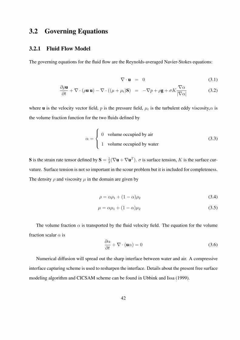
3.2 Governing Equations
3.2.1 Fluid Flow Model
The governing equations for the fluid flow are the Reynolds-averaged Navier-Stokes equations:
∇ · u = 0 (3.1)
∂ρu∂t
+∇ · (ρu u)−∇ · ((µ + µt)S) = −∇p + ρg + σK∇α
|∇α| (3.2)
where u is the velocity vector field, p is the pressure field, µt is the turbulent eddy viscosity,α is
the volume fraction function for the two fluids defined by
α =
0 volume occupied by air
1 volume occupied by water(3.3)
S is the strain rate tensor defined by S = 12(∇u +∇uT ). σ is surface tension, K is the surface cur-
vature. Surface tension is not so important in the scour problem but it is included for completeness.
The density ρ and viscosity µ in the domain are given by
ρ = αρ1 + (1− α)ρ2 (3.4)
µ = αµ1 + (1− α)µ2 (3.5)
The volume fraction α is transported by the fluid velocity field. The equation for the volume
fraction scalar α is∂α
∂t+∇ · (uα) = 0 (3.6)
Numerical diffusion will spread out the sharp interface between water and air. A compressive
interface capturing scheme is used to resharpen the interface. Details about the present free surface
modeling algorithm and CICSAM scheme can be found in Ubbink and Issa (1999).
42

Table 3.1: Constants in k − ε ModelCµ C1 C2 σk σε
0.09 1.44 1.92 1.0 1.3
3.2.2 Turbulence Model
Turbulence in the fluid flow model is estimated by the conventional k-ε two-equation model (Rodi
1993)
µt = Cµρk2
ε(3.7)
∂k
∂t+∇ · (uk) =
1
ρ∇(
µt
σk
∇k) + 2µt
ρ|∇u|2 − ε (3.8)
∂ε
∂t+∇ · (uε) =
1
ρ∇(
µt
σε
∇ε) + 2C1µt
ρ|∇u|2 ε
k− C2
ε2
k(3.9)
where k is the turbulent kinetic energy and ε is the turbulent energy dissipation rate. The constants
in Eqs. 3.7, 3.8 and 3.9 take the values given in Table 3.1.
For wave driven orbital motion, the two equation turbulence models (such as k− ε model) will
become unstable under some conditions. From the authors’ experience, when the wave is strong or
the wave is breaking, instabilities will be observed. Mayer and Madsen (2000) carried out analyt-
ical stability analysis to investigate the erroneous behavior of the turbulence model (k − ω model
in their case) under waves. It turns out that the turbulent eddy viscosity will grow unbounded and
therefore make the model unstable. It seems that no general purpose turbulence model has been
developed especially for unsteady wave driven flows. Most models rely on the tuning of empirical
parameters. For the numerical code used in this research, the values of turbulence parameters are
bounded when they grow out of range (e.g., k and ε become negative). Fortunately, for all the
test cases considered in this work, instability of the turbulence model did not arise. The mod-
ified two-equation turbulence model for wave flows proposed by Mayer and Madsen (2000) or
other modified models can be used when the wave is strong or even breaking and instabilities are
expected.
43

3.2.3 Sediment Transport Model
The scour problem is caused by the erosion movement of sediment. In this numerical model, both
bed load and suspended load are considered. Exner equation is used to update the bed elevation
(Garcıa 1999).
Bed Load Transport
There are many bed load transport rate formulas in the literature. Most of them relate bed load
transport rate with shear stress. The formula of Engelund and Fredsøe (1976) is chosen for the
current model
q∗ =
18.74(θ − θc)[θ1/2 − 0.7θ
1/2c
]if θ > θc
0 otherwise(3.10)
where q∗ is a dimensionless bed load transport rate known as the Einstein number which is given
by
q∗ =q0√Rgdd
Here q0 is the bed load transport rate for flat bed. θ and θc are the Shields number and the critical
Shields number for initiation of motion respectively, where θ is defined as:
θ =τb
ρgRd
Here τb is the bed shear stress calculated with the fluid flow model, ρ is the density of water, g is
the gravitational acceleration, R is the submerged specific gravity of sediment(=1.65 for quartz)
and d is the sediment grain diameter.
The critical Shields number for particular sediment is given for flat bed and should be adjusted
according to the local slope of the bed and local shear force direction. The critical Shields number
for a flat bed, θc0, is a function of flow intensity and sediment properties. θc0 is given as a constant
in most numerical models. The approach used here to account for the slope effect is similar to that
44

used by Roulund et al. (2005). It considered the slope effect and followed the approach suggested
by Engelund and Fredsøe (1976) to use the flow velocity at the particle position and the steepest
slope to adjust the critical Shields number. In this research, the shear stress vector, instead of
velocity near the bed, is used. Fig. 3.1 shows the scheme employed for the adjustment of the bed
shear stress, where n is the surface normal vector, R is the steepest-slope unit vector, and τ is the
wall shear stress vector acting on the bed. The critical Shields number is adjusted according to
θc = θc0
cos β
√1− sin2 φ tan2 β
µ2s
− cos φ sin β
µs
(3.11)
where φ is the angle between the velocity vector and the bed steepest slope direction, β is the slope
angle of the bed. µs is the static friction coefficient and has the value of 0.63 for this work. From
Eq. 3.11, when the wall shear stress tries to move sediment up slope, the critical Shields number
θc increases, and vice versa.
Figure 3.1: Slope Effect on Sediment Transport
Eq. 3.10 only gives the total bed load. The bed load transport rates in different directions are
given by
qi = q0τi
|τ | − C|q0| ∂η
∂xi
, i = 1, 2 (3.12)
where η is the bed elevation, C is a constant in the range of 1.5-2.3 which is used to reflect the
slope effect on the sediment flux (Brørs 1999).
45

Suspended Load
The governing equation for suspended load is a standard convection diffusion equation. Sediment
must be fine enough to ignore the inertial effect of the particle.
∂c
∂t+∇ · (u− vs
g|g|)c = ∇ · (νt∇c) (3.13)
Here c is the sediment concentration, u is fluid velocity vector, vs is sediment fall velocity. νt is
the diffusivity which is taken as the same value as turbulence eddy viscosity.
Bed Morphology Model—Exner Equation
Bed elevation changes are based on the continuity of sediment. The Exner equation, which de-
scribes the sediment continuity, is
∂η
∂t=
1
n− 1[−O · qb + D − E] (3.14)
where η is the bed elevation, n is the porosity of the bed, qb is the bed load transport rate vector
whose components are given by Eq. 3.12. D is the deposition rate and E is the entrainment rate.
The deposition rate D at the bed is
D = vscb (3.15)
where cb is the sediment concentration very near the bed. In the current model, the concentration
at the nearest cell center is used. The entrainment rate E, unlike the deposition rate D, needs some
empirical model. E can be written in dimensionless form as
E =E
vs
(3.16)
Many models are available in the literature for estimating the entrainment rate of sediment into
suspension E. Garcıa and Parker (1991) performed a detailed comparison of eight such relations
46
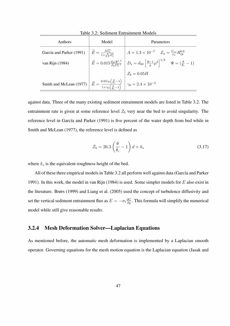
Table 3.2: Sediment Entrainment Models
Authors Model Parameters
Garcıa and Parker (1991) E = AZ5u
1+ A0.3
Z5u
A = 1.3× 10⁻⁷ Zu = U∗svs
R0.6ep
van Rijn (1984) E = 0.015d50Ψ1.5
ZbD0.3∗D∗ = d50
[R−1
g µ2]1/3
Ψ = ( θθc− 1)
Zb = 0.05H
Smith and McLean (1977) E =0.65γ0
(θθc−1
)
1+γ0
(θθc−1
) γ0 = 2.4× 10⁻³
against data. Three of the many existing sediment entrainment models are listed in Table 3.2. The
entrainment rate is given at some reference level Zb very near the bed to avoid singularity. The
reference level in Garcıa and Parker (1991) is five percent of the water depth from bed while in
Smith and McLean (1977), the reference level is defined as
Zb = 26.3
(θ
θc
− 1
)d + ks (3.17)
where ks is the equivalent roughness height of the bed.
All of these three empirical models in Table 3.2 all perform well against data (Garcıa and Parker
1991). In this work, the model in van Rijn (1984) is used. Some simpler models for E also exist in
the literature. Brørs (1999) and Liang et al. (2005) used the concept of turbulence diffusivity and
set the vertical sediment entrainment flux as E = −σt∂C∂y
. This formula will simplify the numerical
model while still give reasonable results.
3.2.4 Mesh Deformation Solver—Laplacian Equations
As mentioned before, the automatic mesh deformation is implemented by a Laplacian smooth
operator. Governing equations for the mesh motion equation is the Laplacian equation (Jasak and
47

Tukovic 2007). Let v be the grid motion velocity field, then the equation becomes
∇ · (γ∇v) = 0 (3.18)
where γ is the diffusion coefficient chosen to control the mesh motion. γ can be a constant or
a variable defined by other properties in the domain. The selection of variable γ depends on the
specific mesh motion problem and needs objective judgment. Jasak and Tukovic (2007) suggested
several possibilities to set the γ value based on distance (linear, quadratic and exponential) from
some boundary or mesh characteristics (orthogonality and skewness). These methods all have their
merits and shortcomings. In this work, γ is set as a non-zero constant for simplicity. The boundary
condition for Eq. 3.18 is given by the Exner equation. After each time step of bed elevation change,
the bed grid motion velocity is known. When the grid motion velocity field is solved, the grids in
the whole domain can be moved based on the following equation
xk+1 = xk + v∆t (3.19)
Here, xk+1 and xk are grid position vectors at time level k + 1 and k respectively, and ∆t is the
time step.
Fig. 3.2 is a simple test case for the mesh deformation component of the numerical model. The
bottom of a rectangular flume (with unstructured grid) is ”vibrating” in a sinusoidal mode with a
period T = 0.8 s. Mesh grids at t = 0, T/4, T/2 and 3T/4 are shown. In real cases, the bed will
move in a more complicated way.
3.3 Numerical Simulation Schemes and Procedures
The governing equations presented in the previous section form a strongly coupled system of
equations. The solution of this system of equations needs some effort because even for each
single component (fluid, free surface or sediment) is a difficult problem. Also the time scales of
48
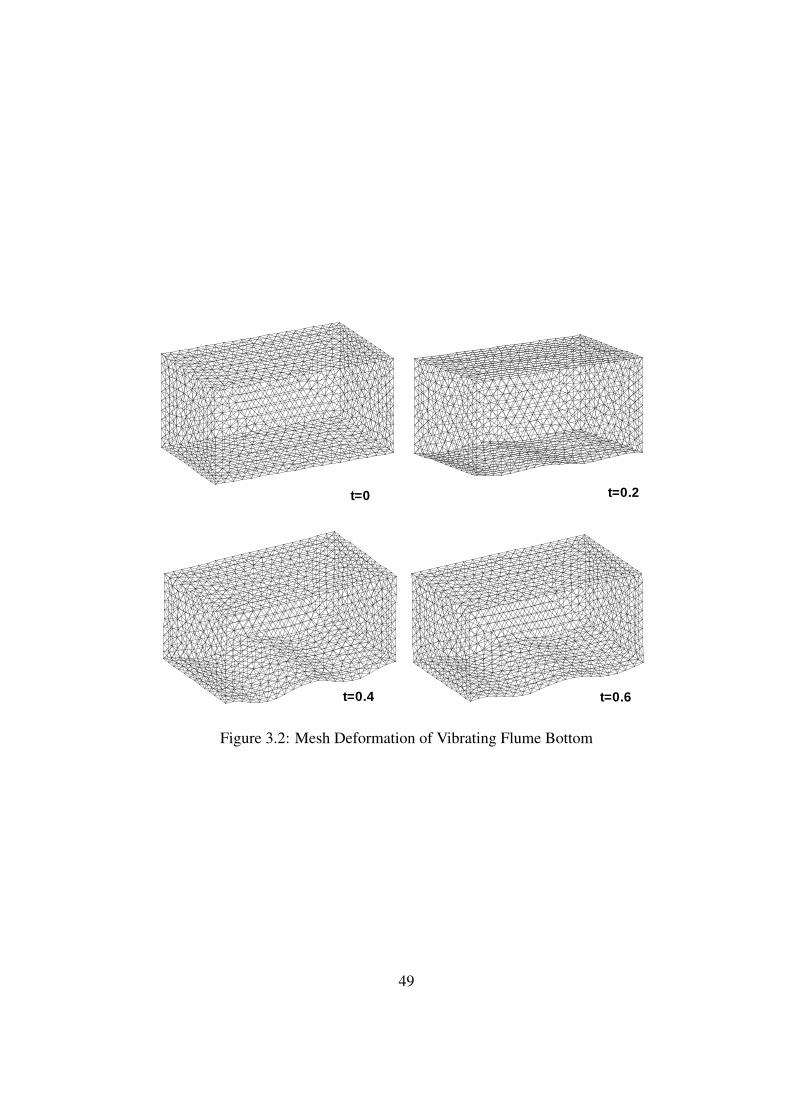
t=0.4 t=0.6
t=0.2t=0
Figure 3.2: Mesh Deformation of Vibrating Flume Bottom
49

the flow field and sediment transport are so largely different that the whole system is very stiff.
Consequently, numerical instabilities can be expected to arise. The emphasis of this research is
not on the numerical details but on building a numerical model for the local scour problem and
verification of the numerical solution of the model. So numerical schemes for each component
of this system are described only briefly. Several references about these numerical schemes are
provided for the interested readers.
The code used in this work is an open source computational fluid dynamics (CFD) code named
OpenFOAM (OpenCFD 2006). It is freely available through internet. OpenFOAM is primarily
designed for problems in continuum mechanics. It uses the tensorial approach and object ori-
ented techniques (Weller et al. 1998). OpenFOAM provides a fundamental platform to write new
solvers for different problems as long as the problem can be written in tensorial partial differential
equation form. Here, the flow field is solved by the adaption of the original turbulence solver for
incompressible fluid. The sediment transport equation and bed deformation are added to the fluid
flow solver to form a new solver called FOAMSCOUR. The core of this code is the finite volume
discretization of the governing equations. Almost all kinds of differential operators possible in a
partial differential equation, such as temporal derivative, divergence, laplacian operator, curl, etc,
can be discretized in the code. The finite volume details of the code can be found in Jasak (1996).
The next section is a brief introduction of the numerical scheme used in FOAMSCOUR.
3.3.1 Numerical Scheme for the Flow Field
The numerical solution of the Navier-Stokes equation for incompressible fluid flow imposes two
main problems (Jasak 1996): the nonlinearity of the momentum equation and the pressure-velocity
coupling. For the first problem, two common methods can be used to deal with it. The first is to
solve a nonlinear algebraic system after the discretization. This will need a lot of computational
effort. The other is to linearize the convection term in the momentum equation by using the fluid
velocity in previous time steps which satisfies the divergence-free condition. The latter method
is used in this research. For pressure-velocity coupling, many schemes exist, such as the semi-
50

implicit method for pressure linked equation (SIMPLE) (Patankar 1981) and pressure implicit
splitting of operators (PISO) (Issa 1986). PISO scheme is used in this code. For the k−ε turbulence
model equations, although k and ε equations are coupled together, they are solved by a segregated
approach, which means they are solved one at a time. This is also the usual approach used in most
CFD codes.
For the free surface, CICSAM scheme is easy to code and captures the free surface fairly well.
But the problem with this scheme is that it is very slow. The time step required is so small that
the computation usually takes a very long time even for a small computational domain. This is
partially caused by the fact that the control cell which has the largest Courant number usually is
in the air phase. In our case, the two phases are water and air. The density of water is almost
1000 times larger than that of air and the velocity magnitude in the air phase is far greater than
in the water phase. A modified approach is proposed in this work analog to those used in other
CFD codes. The aim is to relax the time step requirement while capturing the free surface. In the
modified approach, the volume occupied by the air phase can be called void. In the void region,
the velocity is set to zero and the pressure is set to atmospheric pressure. This will not upset the
computations because of the large density ratio between water and air. The inertia force associated
with air can thus be neglected. The threshold value of α for the void (i.e., below what value
of α, it can be viewed as void) needs some consideration. The classical dam break problem is
carried out to investigate the effect of the threshold value. As in Fig. 3.3(a), a column of water
is released at time t = 0 s and an obstacle is located in front of the water column. Fig. 3.3 shows
the contour of the VOF scalar α which is the volume fraction of water. The results at t = 0.3 s for
different threshold values (0.01 and 0.1) are plotted together with the original scheme (threshold
value equals 0). The result from threshold value 0.01 is very close to the original scheme while that
from threshold value 0.1 causes more damping of the water flow. This is because high threshold
values imply that a larger portion of the flow field is set to zero velocity and the water needs to
consume more energy to go through such area. In this work, a threshold value 0.01 is used for all
computations and the computational time is reduced by almost half.
51
(a) (b)
(c) (d)
Figure 3.3: Test Cases for Modified CICSM Scheme (a) Initial state (b) Critical α = 0 (c) Criticalα = 0.01 (d) Critical α = 0.1
52
3.3.2 Numerical Scheme for the Sediment Transport
The bed load and suspended load in the sediment transport modules are solved separately. Since
the shear stress on the bottom is obtained from the flow solver, using Eq. 3.10 to calculate the bed
load is straightforward. The suspended load equation (Eq. 3.13) is a convection-diffusion equation
and the sediment is transported passively by the flow field. Finite volume method is also used to
solve this equation.
After the sediment load (namely bed load and suspended load) is calculated, the Exner equation
is solved to change the bed elevation. Exner equation is a 2D equation although the bed is in
3D space. This is because the vertical coordinate z is the variable to be solved and it is not an
independent variable any more. The bed elevation change is due to the divergence of sediment
transport flux together with erosion and deposition of sediment on the bed surface. This simple
2D equation can usually be solved by the finite difference method using a structured grid when
the bottom has a regular shape (Beek and Wind 1990; Olsen and Melaaen 1993; Brørs 1999;
Olsen and Melaaen 1999). For complex domains, such as a natural river bottom or in the presence
of objects (bridge piers, break water etc.), a finite volume or finite element method can be used
with unstructured grids. In this research, two meshes are used. One is for the fluid flow solver
and the other is for the bottom Exner equation. The Exner equation is solved on the 2D mesh
using finite volume method. In Fig. 3.4, it is shown that the coupled problem is solved through
mapping between the fluid mesh bottom boundary and sediment 2D mesh. After the flow solver
and turbulence solver are finished, the shear stress and other parameters are available. Those flow
parameters are mapped from the 3D fluid bottom boundary to the 2D bed sediment mesh. On the
2D sediment mesh, the Exner equation is solved and the new bed elevation is calculated. Then
the bed elevation is mapped back from 2D sediment mesh to 3D fluid mesh. The 3D fluid mesh
is deformed according to this as a boundary condition. The use of separate meshes for the flow
field and the Exner equation keeps the concept clear and easy to manage in the code. Mapping
back and forth between these two meshes could lead to loss of some accuracy when averaging and
53

interpolation are needed. But when the mesh is sufficiently fine or the mapping is almost one to
one, accuracy is not a problem.
3D Fluid MeshBoundary Patch
2D Bed Mesh
Mapping
Figure 3.4: Mapping between 3D and 2D Bed Mesh
3.3.3 Numerical Scheme for Automatic Mesh Deformation
The Laplacian equation in Eq. 3.18 needs to be solved on the 3D mesh to get the movement
of each node. Finite element method (FEM, which is implemented in the original OpenFOAM
package), the finite volume method as well as other numerical methods can be used. In the original
OpenFOAM package, each cell of the 3D mesh is decomposed into tetrahedral elements and the
new refined mesh is used to solve the Laplacian equation. The details of the FEM implementation
can be found in OpenCFD (2006) and Jasak and Tukovic (2007). This built-in FEM method is very
slow especially when the 3D mesh is very big. Numerical tests show that the decomposition time
is almost half that of total mesh motion solution step. Also the decomposition makes the new mesh
much larger (usually several times the original mesh size) and therefore makes the computation
even longer. In this work, some simplifications are made according to the unique character of the
problem under consideration. For the scour problem in this work, the specific characteristic is that
the sand bed boundary movement is in the vertical direction (deposition or erosion). This makes
54
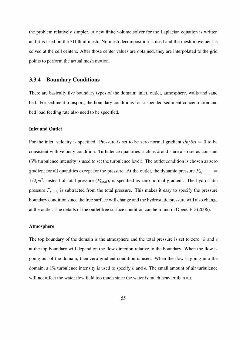
the problem relatively simpler. A new finite volume solver for the Laplacian equation is written
and it is used on the 3D fluid mesh. No mesh decomposition is used and the mesh movement is
solved at the cell centers. After those center values are obtained, they are interpolated to the grid
points to perform the actual mesh motion.
3.3.4 Boundary Conditions
There are basically five boundary types of the domain: inlet, outlet, atmosphere, walls and sand
bed. For sediment transport, the boundary conditions for suspended sediment concentration and
bed load feeding rate also need to be specified.
Inlet and Outlet
For the inlet, velocity is specified. Pressure is set to be zero normal gradient ∂p/∂n = 0 to be
consistent with velocity condition. Turbulence quantities such as k and ε are also set as constant
(5% turbulence intensity is used to set the turbulence level). The outlet condition is chosen as zero
gradient for all quantities except for the pressure. At the outlet, the dynamic pressure Pdynamic =
1/2ρu2, instead of total pressure (Ptotal), is specified as zero normal gradient. The hydrostatic
pressure Pstatic is subtracted from the total pressure. This makes it easy to specify the pressure
boundary condition since the free surface will change and the hydrostatic pressure will also change
at the outlet. The details of the outlet free surface condition can be found in OpenCFD (2006).
Atmosphere
The top boundary of the domain is the atmosphere and the total pressure is set to zero. k and ε
at the top boundary will depend on the flow direction relative to the boundary. When the flow is
going out of the domain, then zero gradient condition is used. When the flow is going into the
domain, a 1% turbulence intensity is used to specify k and ε. The small amount of air turbulence
will not affect the water flow field too much since the water is much heavier than air.
55
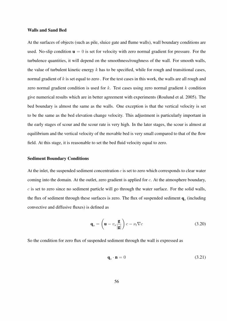
Walls and Sand Bed
At the surfaces of objects (such as pile, sluice gate and flume walls), wall boundary conditions are
used. No-slip condition u = 0 is set for velocity with zero normal gradient for pressure. For the
turbulence quantities, it will depend on the smoothness/roughness of the wall. For smooth walls,
the value of turbulent kinetic energy k has to be specified, while for rough and transitional cases,
normal gradient of k is set equal to zero . For the test cases in this work, the walls are all rough and
zero normal gradient condition is used for k. Test cases using zero normal gradient k condition
give numerical results which are in better agreement with experiments (Roulund et al. 2005). The
bed boundary is almost the same as the walls. One exception is that the vertical velocity is set
to be the same as the bed elevation change velocity. This adjustment is particularly important in
the early stages of scour and the scour rate is very high. In the later stages, the scour is almost at
equilibrium and the vertical velocity of the movable bed is very small compared to that of the flow
field. At this stage, it is reasonable to set the bed fluid velocity equal to zero.
Sediment Boundary Conditions
At the inlet, the suspended sediment concentration c is set to zero which corresponds to clear water
coming into the domain. At the outlet, zero gradient is applied for c. At the atmosphere boundary,
c is set to zero since no sediment particle will go through the water surface. For the solid walls,
the flux of sediment through these surfaces is zero. The flux of suspended sediment qs (including
convective and diffusive fluxes) is defined as
qs =
(u− vs
g|g|
)c− νt∇c (3.20)
So the condition for zero flux of suspended sediment through the wall is expressed as
qs · n = 0 (3.21)
56

At the sand bed, the suspended sediment flux is specified as the net upward normal flux
qs · n = E −D (3.22)
where D is defined in Eq. 3.15 and E is calculated by using the empirical model by van Rijn
(1984) as shown in Table 3.2.
Bed load boundary conditions are defined similarly. At the inlet, bed load is set to be zero
which corresponds to zero feeding rate because of the concrete bed before flow hits the sand bed
(see the test case section). At the outlet, zero gradient is applied. At the wall surfaces, the bed load
flux is set to zero as for suspended load, i.e.
qb · n = 0 (3.23)
3.3.5 Simulation Flow Chart
The flow chart for the simulation process is plotted in Fig. 3.5. A quasi-steady approach is used
in the model. In this approach, it is assumed the time scale of bed change is far larger than that
of flow field and the time steps for flow field and morphological calculations are different. When
the flow field is being calculated, the domain boundaries are fixed. Only at the sediment transport
step, the domain boundaries are adjusted. A scheme similar to the method proposed by Liang et al.
(2005) is used here. During the simulation, m time steps of flow field simulation are carried out
between the morphological steps. This approximation is only valid when the bed changes are very
slow when compared to the flow changes. Through numerical experiments, it is found that at the
beginning of the local scour process, the bed changes very rapidly and most of the scour occurs
in this stage. In order to increase the accuracy, smaller values of m are used at the beginning of
the simulation. After the flow field and bed change reach relatively steady state, bigger values of
m can be used to accelerate the computation. In the test cases considered here, m = 1 is used
at the initial stage of simulation and m gradually increases to 100 when the whole system tends
57

to equilibrium. There are some differences between the current time marching scheme and the
one in Liang et al. (2005). Liang et al. (2005) only use k, where k < m, time steps between
morphological steps and assume that from time step k + 1 to m, the flow field does not change
much. The flow field from time step k is used to perform the morphological calculation. This will
further reduce the computational time.
Figure 3.5: Flow Chart of Computational Scheme
3.4 Model Verification and Applications
In this section, applications of turbulent wall jet scour (2D case) and wave scour around a large
vertical circular cylinder (3D case) are carried out using FOAMSCOUR and the numerical results
are compared with experiments. In turbulent wall jet scour process, the jet flow and momentum
diffusion are of interest as both have an impact on the scour hole development. In wave scour
around a large pile, the water wave and its interaction with the pile and bed sediment are impor-
tant. The coupled problems of flow field and morphodynamics usually take a very long time for
computation. Parallel computation with domain decomposition is used to accelerate the process.
OpenFOAM comes with parallel computing support and FOAMSCOUR easily uses these mod-
58

ules to implement both flow field solver and sediment transport solver. All computations were
done on the National Center for Supercomputing Applications (NCSA) Tungsten Xeon Cluster at
the University of Illinois at Urbana-Champaign.
3.4.1 Wall Jet Scour Test Case
The experimental data of turbulent wall jet scour by Chatterjee and Ghosh (1980) and Chatterjee
et al. (1994) are used. This experiment investigated the flow field and sediment transport due to a
submerged wall jet. The schematic view of the experiment is shown in Fig. 3.6. The jet is formed
by a small opening under a sluice gate and flows over a rigid apron onto an erodible bed. The
details of the experiment can be found in the original papers. Run2 of the experiment is chosen as
a typical run to be simulated. The bed material is sand with d50 = 0.76 mm, submerged specific
gravity 1.65, porosity 0.43 and angle of repose 29 degrees. The flow condition for this run is
as follows. The apron length is 0.66 m and the jet inlet velocity is 1.56 m/s. The downstream
water depth is controlled to be 0.291 m by the outlet weir. In the experiment, the jet inlet velocity
is caused by the difference between upstream and downstream water depth. The corresponding
water depth difference in Run2 is 0.118 m. But in this simulation, the conditions upstream of the
sluice gate are not modeled. Equivalently, velocity is specified at the jet inlet. Although the test
case is 3D, the flume side walls have little effect on the main region of the flow and the scour
profile is almost uniform in the span wise direction.
Figure 3.6: Turbulent Wall Jet Scour Schematic View
59

In Fig. 3.7, free surface and velocity magnitude contours at equilibrium state are plotted. When
the jet flow starts, it induces water waves in the domain. After the flow calms down, the free surface
keeps an almost steady position. The free surface at the equilibrium state is almost flat except in
the region of maximum scour. The velocity magnitude contours show that the jet flow comes into
the domain through the small opening and after momentum diffusion and water entrainment it
leaves the domain through free fall over the outlet weir.
Figure 3.7: Numerical Results for Turbulent Wall Jet Flow Field and Free Surface
The stream trace in the region of jet opening and scour hole at equilibrium state is plotted in
Fig. 3.8. The flow pattern is more clearly shown. The jet induces strong flow re-circulation and
just above the jet inlet, there are some small circulation areas which are isolated from the main
flow. Inside the scour hole, the stream trace lines show another circulation pattern. These flow
patterns are closely related to the scour process. When the water leaves the jet orifice, the main
physical processes are the momentum diffusion and entrainment of water from above into the jet
flow. As a result, the magnitude of the maximum velocity and also the velocity distribution will be
60
x(m)
y(m
)
0 0.1 0.2 0.3 0.4 0.5 0.6 0.7 0.8 0.9 1 1.1 1.2 1.3 1.4-0.1
0
0.1
0.2
0.3
0.4
0.5
Free Surface
Jet Inlet Scour Hole
Figure 3.8: Numerical Results for Turbulent Wall Jet Flow Stream Trace
changed. This change is a complicated function of flow domain geometry and sediment properties
(Chatterjee and Ghosh 1980). In Fig. 3.9(a), the maximum horizontal velocity normalized by jet
inlet velocity is plotted against the non-dimensionalized x distance where B0 is the jet opening
width. The wall jet momentum diffusion characteristics found in experiment are reproduced well
by the numerical simulation. As in the experiment, the diffusion process is slower in the rigid apron
region than in the erodible bed region. In the near jet opening region, the numerical results are very
close to the experimental data. But in the far down stream region, the momentum diffusion is over
estimated by the numerical simulation, i.e., the maximum velocity is smaller and the velocity
distribution in the vertical direction is more uniform. This may come from the numerical diffusion
nature of the schemes used in this test case.
Wall jet flow near the jet opening can be divided into two regions. One is the inner boundary
layer region and the other is the outer shear layer region. When the boundary layer meets the shear
layer, the potential core will disappear and the jet flow is fully developed (Rajaratnam 1976). The
61
1 2 3 4 5 6 7 8 910 20 30 40 50600.1
0.2
0.4
0.6
0.81
2
U/U
0
x/B0
experiment data numerical results
(a)
0 1 2 3 4 5 6 7 8 9 10 11 12 13-0.10.00.10.20.30.40.50.60.70.80.91.01.11.2
f()=
u/U
=(y/ )
experiment data numerical result
(b)
Figure 3.9: Turbulent Wall Jet Characteristic: (a) Jet Diffusion along x-Axis (b) Velocity Distribu-tion at x=0.6m
horizontal velocity at location x = 0.6 m downstream of the jet opening is plotted in Fig. 3.9(b).
In Fig. 3.9(b), ξ is defined as y/δ, where δ is the vertical distance from the wall to location of the
maximum horizontal velocity. Non-dimensionalized velocity is plotted as a function of ξ. From
Fig. 3.9(b), the numerical simulation predicted the velocity distribution fairly well.
Fig. 3.10 shows the mesh development from the initial flat bed condition to the equilibrium
configuration. The unstructured mesh is composed of three layers of fine quadrilateral cells in the
boundary layer on the bottom and triangle cells elsewhere. With the change of bottom elevation due
to scour and deposition, the computational domain gradually deforms while the unstructured mesh
remains valid. There is a small artificial step at the transition point between the concrete apron and
the sand bed. It has a depth of 5 mm. This small step is used to improve the mesh quality because
the scour hole will make the cells in front of the transition point vertically stretched. Inside the
small step, several mesh cells are introduced making the simulation stable.
Scour profiles from numerical simulation at different times are plotted in Fig. 3.11 as solid
lines together with the experimental results. The time required to get to equilibrium state is almost
one hour for this test case. Fig. 3.12 shows the time development of the maximum scour and
deposition. At equilibrium state, according to the numerical simulation results, the maximum
62

x (m)
y(m
)
0.6 0.7 0.8 0.9 1 1.1 1.2 1.3 1.4-0.1
0
0.1
0.2
0.3
0.4
0.5
(a)
x (m)
y(m
)
0.6 0.7 0.8 0.9 1 1.1 1.2 1.3 1.4-0.1
0
0.1
0.2
0.3
0.4
0.5
(b)
Figure 3.10: Turbulent Wall Jet Scour Mesh Deformation: (a) Initial (b) Equilibrium
63

scour depth is about 0.63 m and the maximum deposition depth is about 0.4 m. These fit well with
the observations made in the experiment. From Fig. 3.12, the scour process occurs very rapidly in
the early stage while at later stage, the profile changes very slowly. The maximum scour position
and the peak of the sediment deposition dune move very slowly downstream.
-0.1 0.0 0.1 0.2 0.3 0.4 0.5 0.6 0.7-0.07-0.06-0.05-0.04-0.03-0.02-0.010.000.010.020.030.040.050.060.070.08
h(m)
x(m)
Experimental Data: t=1min t=3min t=5min t=8min t=12min t=20min t=30min t=60min
Original Bed Level
Figure 3.11: Wall Jet Scour Profile
0 10 20 30 40 50 60 70
0.02
0.03
0.04
0.05
0.06
0.07
Scou
r Dep
th (m
)
Time (min)
Experiment Maximum Scour Numerical Maximum Scour
(a)
0 10 20 30 40 50 60 70
0.02
0.03
0.04
0.05
0.06
0.07
Dep
ositi
on H
eigh
t (m
)
Time (min)
Experiment Maximum Deposition Numerical Maximum Deposition
(b)
Figure 3.12: Wall Jet Maximum Scour and Deposition Development with Time: (a) MaximumScour (b) Maximum Deposition
In Fig. 3.13, the Shields number at equilibrium state is plotted. Chatterjee and Ghosh (1980)
gave an estimation of critical shear stress along the bed using von Karman’s integral theorem. But
64
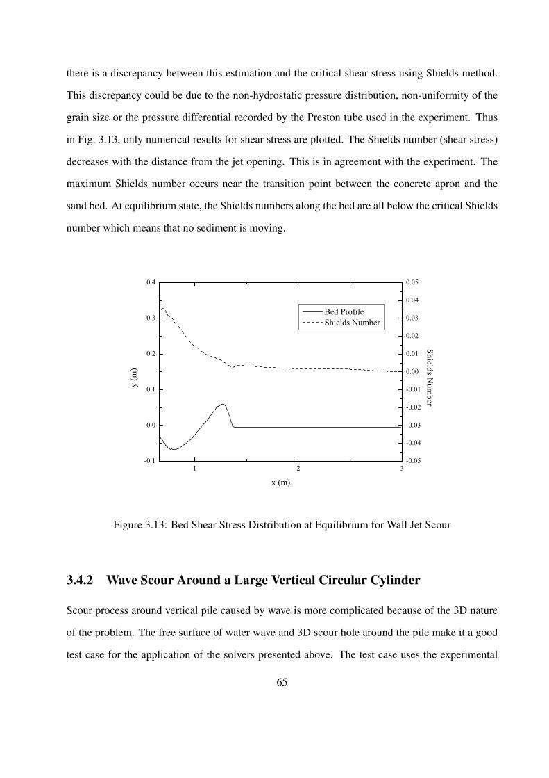
there is a discrepancy between this estimation and the critical shear stress using Shields method.
This discrepancy could be due to the non-hydrostatic pressure distribution, non-uniformity of the
grain size or the pressure differential recorded by the Preston tube used in the experiment. Thus
in Fig. 3.13, only numerical results for shear stress are plotted. The Shields number (shear stress)
decreases with the distance from the jet opening. This is in agreement with the experiment. The
maximum Shields number occurs near the transition point between the concrete apron and the
sand bed. At equilibrium state, the Shields numbers along the bed are all below the critical Shields
number which means that no sediment is moving.
1 2 3-0.1
0.0
0.1
0.2
0.3
0.4
Bed Profile Shields Number
x (m)
y (m
)
-0.05
-0.04
-0.03
-0.02
-0.01
0.00
0.01
0.02
0.03
0.04
0.05
Shields Num
ber
Figure 3.13: Bed Shear Stress Distribution at Equilibrium for Wall Jet Scour
3.4.2 Wave Scour Around a Large Vertical Circular Cylinder
Scour process around vertical pile caused by wave is more complicated because of the 3D nature
of the problem. The free surface of water wave and 3D scour hole around the pile make it a good
test case for the application of the solvers presented above. The test case uses the experimental
65

data obtained by Sumer and Fredsøe (2001). The schematic view of the experiment is shown in
Fig. 3.14. Test case 7 of the experiment is used in this work. In this case, the wave has a period
of 3.5 s, wave height of 6.4 cm, wave length of 6.79 m and Keulegan-Carpenter (KC) number of
0.61. The pile has a diameter of 1 m and the sand has d50 = 0.2 mm.
The mechanism causing the scour around a vertical pile can be different under different con-
ditions. Flow regimes change when the dimensionless number KC (Keulegan-Carpenter number)
increases. KC number is defined as
KC =UmT
D(3.24)
where Um is the maximum undisturbed orbital velocity at the bed. When the pile is slender, the
scour is primarily caused by vortex shedding (KC < O(100)) and by horseshoe vortex (KC >
O(100)) (Sumer et al. 1992; 1993). For this case, the free surface is of secondary importance and
can be replaced by a rigid lid. Numerical simulations using the rigid-lid approximation captured
the vortex shedding and horseshoe vortex well and gave good results (Roulund et al. 2005). When
the pile diameter is big enough, the scour is caused by the combined effect of phase-resolved
component of the wave flow and the steady streaming due to the presence of the large cylinder
(Sumer and Fredsøe 2001). For this case, the modeling of the free water surface is very important.
Without the free surface, the steady streaming can not be correctly simulated and the scour process
can not be captured.
The waves in the experiment are generated by a piston type wave maker and at the end of the
wave tank, there is a wave absorber to eliminate wave reflection. The details of the experiment can
be found in the original paper. In the numerical simulations, the wave can be generated generally
by two approaches: moving mesh (Aliabadi et al. 2003) and wave boundary condition (Mayer et al.
1998). For the moving mesh approach, the piston movement is simulated by moving the boundary
of the computational domain. For the wave boundary condition approach, the mesh is fixed but
boundary condition on the piston part is given by wave theory. The second approach is adopted in
this work. A time varying velocity profile is imposed at the piston boundary to generate the waves
66

Figure 3.14: Wave Scour around a Large Vertical Circular Cylinder Scheme (After Sumer andFredsøe (2001) With Permission)
U = fr(t) [U(y)sin(ωt + θ)] (3.25)
where U is the velocity vector at the boundary, ω is the wave frequency, θ is the phase. U(y) is
imposed by the type of the piston. In the test case, the relative depth h/L and wave steepness H/L
are about 1/17 and 1/106 respectively. The linear wave maker theory applies and for the piston
type wave maker in this case, U(y) is a constant (Dean and Dalrymple 1991). For finite amplitude
wave cases, nonlinear effect is important and higher order terms need to be added. fr(t) is the
”ramp” function to start up the piston. fr(t) has the form
fr(t) =
tT− 1
πsin
(π t
T
)for 0 < t < T
1 for t > T(3.26)
where T is the wave period.
The wave absorber is simulated using a damping zone (or sponge layer). In this damping zone,
wave energy is artificially dissipated and wave reflection is minimized. The water depth and fluid
67
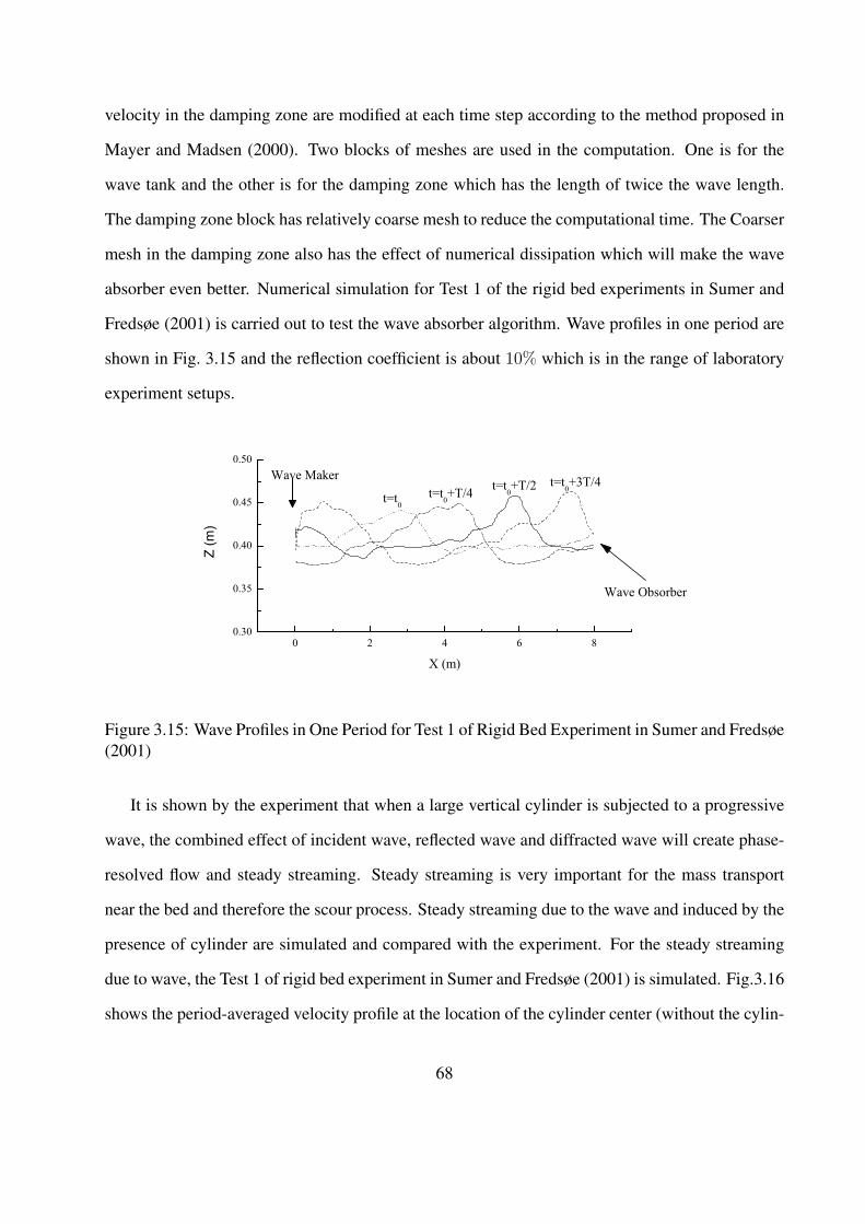
velocity in the damping zone are modified at each time step according to the method proposed in
Mayer and Madsen (2000). Two blocks of meshes are used in the computation. One is for the
wave tank and the other is for the damping zone which has the length of twice the wave length.
The damping zone block has relatively coarse mesh to reduce the computational time. The Coarser
mesh in the damping zone also has the effect of numerical dissipation which will make the wave
absorber even better. Numerical simulation for Test 1 of the rigid bed experiments in Sumer and
Fredsøe (2001) is carried out to test the wave absorber algorithm. Wave profiles in one period are
shown in Fig. 3.15 and the reflection coefficient is about 10% which is in the range of laboratory
experiment setups.
0 2 4 6 80.30
0.35
0.40
0.45
0.50
Wave Obsorber
t=t0+3T/4t=t
0+T/2t=t
0+T/4
Z (m
)
X (m)
t=t0
Wave Maker
Figure 3.15: Wave Profiles in One Period for Test 1 of Rigid Bed Experiment in Sumer and Fredsøe(2001)
It is shown by the experiment that when a large vertical cylinder is subjected to a progressive
wave, the combined effect of incident wave, reflected wave and diffracted wave will create phase-
resolved flow and steady streaming. Steady streaming is very important for the mass transport
near the bed and therefore the scour process. Steady streaming due to the wave and induced by the
presence of cylinder are simulated and compared with the experiment. For the steady streaming
due to wave, the Test 1 of rigid bed experiment in Sumer and Fredsøe (2001) is simulated. Fig.3.16
shows the period-averaged velocity profile at the location of the cylinder center (without the cylin-
68
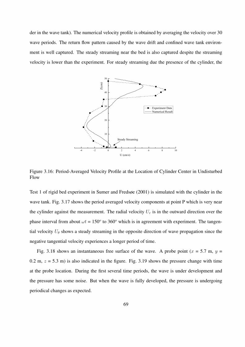
der in the wave tank). The numerical velocity profile is obtained by averaging the velocity over 30
wave periods. The return flow pattern caused by the wave drift and confined wave tank environ-
ment is well captured. The steady streaming near the bed is also captured despite the streaming
velocity is lower than the experiment. For steady streaming due the presence of the cylinder, the
-4 -2 0 2 4 6 8 100
10
20
30
40
50
Z(cm
)
U (cm/s)
Experiment Data Numerical Result
Steady Streaming
Figure 3.16: Period-Averaged Velocity Profile at the Location of Cylinder Center in UndisturbedFlow
Test 1 of rigid bed experiment in Sumer and Fredsøe (2001) is simulated with the cylinder in the
wave tank. Fig. 3.17 shows the period averaged velocity components at point P which is very near
the cylinder against the measurement. The radial velocity Ur is in the outward direction over the
phase interval from about ωt = 150o to 360o which is in agreement with experiment. The tangen-
tial velocity Uθ shows a steady streaming in the opposite direction of wave propagation since the
negative tangential velocity experiences a longer period of time.
Fig. 3.18 shows an instantaneous free surface of the wave. A probe point (x = 5.7 m, y =
0.2 m, z = 5.3 m) is also indicated in the figure. Fig. 3.19 shows the pressure change with time
at the probe location. During the first several time periods, the wave is under development and
the pressure has some noise. But when the wave is fully developed, the pressure is undergoing
periodical changes as expected.
69
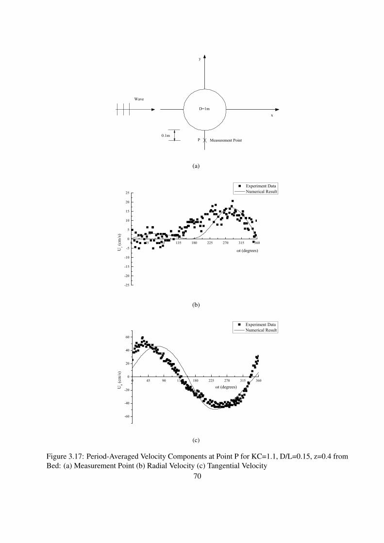
x
y
D=1m
Wave
P Measurement Point0.1m
(a)
0 45 90 135 180 225 270 315 360
-25
-20
-15
-10
-5
0
5
10
15
20
25
Experiment Data Numerical Result
Ur (c
m/s
)
t (degrees)
(b)
0 45 90 135 180 225 270 315 360
-60
-40
-20
0
20
40
60
Experiment Data Numerical Result
U (c
m/s
)
t (degrees)
(c)
Figure 3.17: Period-Averaged Velocity Components at Point P for KC=1.1, D/L=0.15, z=0.4 fromBed: (a) Measurement Point (b) Radial Velocity (c) Tangential Velocity
70

Figure 3.18: Free Surface of the Wave around Pile
0 5 10 15 20 25 30 35 40 45 50 55 603500
4000
4500
5000
5500
6000
6500
7000
7500
Pres
sure
(Pa)
Time (s)
Developing Developed
Figure 3.19: Pressure Probe at Point (x = 5.7 m, y = 0.2 m, z = 5.3 m)
71

Fig. 3.20 shows the equilibrium state of the scour around the pile. The numerical result is com-
parable with the experimental data although the maximum scour depth obtained with the numerical
simulation is slightly higher than the experiment result. As in the experiment, the deposition zone
is on the side of the pile and the scour zone is in the front and in the back. Although the scour
pattern is not identical to that of the experimental results, they are very similar. Fig. 3.21 shows
the scour around the periphery of the cylinder base. Only half of the periphery is shown because
of symmetry. From this figure, the scour and deposition patterns around the pile are seen to agree
well with the experiment except for the amplitude. This may be caused by the fact that some other
factors in the experiment are not included in the numerical model. Further research is needed to
make the model more accurate.
3.5 Discussion
3.5.1 Effect of Free Surface
For the rigid-lid approach, the free surface is replaced with an imaginary horizontal frictionless
plane. In reality, even when the free surface is almost flat and will not change with time, a rea-
sonable position for the free surface is not easy to be defined. This is because locally, such as in
the case of free surface around a bridge pier, the free surface may change very abruptly and the
rigid-lid approach simply can not capture these features. On the other hand, for the submerged
wall jet case, the water depth in the flow domain is much bigger than the jet opening and the free
surface changes very slowly. This makes the rigid-lid approximation a reasonable one. For scour
around slender piles under waves, the rigid-lid assumption is also valid since the most important
mechanism here is the vortex shedding and horseshoe vortex. However, for the wave-induced
scour around large piles, it’s unreasonable to use the rigid-lid approximation since the dominant
mechanism here is the phase-resolved component of the wave flow and the steady streaming.
72

-1.0 -0.5 0.0 0.5 1.0
-1.0
-0.5
y(m)
x(m)
Wave
-1
+1
+1.5
0
+1
-1
-1.5
0
-1
-2cm
(a)
-1.0 -0.5 0.0 0.5 1.0
-1.0
-0.5
-1
y(m)
x(m)
-1-1
0
+1
+2+3
-2
-2cm
-3
0
(b)
(c)
Figure 3.20: Wave Scour around a Large Vertical Circular Cylinder: (a) Experimental Data (b)Numerical Result (c) 3D View of Numerical Result
73

-0.05
-0.04
-0.03
-0.02
-0.01
0.00
0.01
0.02
0.03
0.04
0.05
S/D
Numerical Experimental
X
23 /2
Figure 3.21: Scour at Periphery of Cylinder Base
3.5.2 Interface Capturing Techniques
In the current numerical model, the two moving surfaces (water free surface and moving bed) are
captured by different approaches, namely Eulerian and Lagrangian approaches. The free surface
is solved by CICSAM VOF scheme, which is an Eulerian approach. The moving bed is captured
by mesh deformation method, which is a Lagrangian approach. The scour test cases in this work
are relatively simple. For more complicated problems, if there are objects interacting with the fluid
phase and the bed, the moving mesh technique will not be appropriate. The interface between the
object, water and bed is so complicated and changing with time. Simply moving a grid point along
the interface will be not feasible. For such cases, the Eulerian approach (VOF or LSM) can be used
to implicitly track the interface. This could provide a new research direction in the scour problem
and is currently being explored.
74
3.5.3 Limitation of Mesh Deformation Approach
As mentioned in the previous section, the mesh deformation approach is hard to implement with
the presence of interaction between moving objects and bed or when the boundary movement is
irregular. Also when the amplitude of the boundary movement is big enough, the mesh may be
highly distorted and the deteriorated mesh quality will make the computation not easy to converge,
eventually leading to unstable solutions. In order to avoid these problems, dynamic mesh approach
should be used. In dynamic mesh approach, mesh cells can be split or merged when necessary.
But comparing with mesh deformation, dynamic mesh approach is more difficult. Combination of
these two approaches can be promising for scour problem where scour pattern is complicated and
the scour/deposition depth is very large.
3.6 Conclusions
Numerical model FOAMSCOUR for local scour with free surface and automatic mesh deformation
is proposed. The turbulence model used is the simple two equation k − ε model. Other turbulence
models, even large eddy simulation, can be used to improve the accuracy of the fluid flow field
simulation. All these models are readily implemented in OpenFOAM. The free surface is modeled
by VOF method while the scour process is modeled by moving mesh method. These two methods
for moving boundaries(free surface and bed) are coupled together. Each method has its merits
and shortcomings. Eulerian approach can be used to capture the complex scour profiles. Flow
field is coupled with sediment transport (both bed load and suspended load) using a quasi-steady
approach. Parallel computations are used to reduce the CPU time which is usually tremendously
large for morphological simulations (Parker and Garcıa 2006).
Numerical simulations for turbulent wall jet scour and wave scour around large vertical cylin-
der are carried out to compare with experiments. Good results have been obtained using the pro-
posed modeling approach. Velocity field and other flow field characteristics compare fairly well
with experimental observations. The maximum scour depths and local scour profile fit well with
75
the experiment data. Further research is needed to investigate the effect of turbulence model for
free surface waves (especially for near breaking and breaking waves) and to study the possibility
of using an Eulerian approach for morphological modeling.
76

Chapter 4
Three-Dimensional Numerical Model forMomentary Liquefaction Potential underWaves
4.1 Introduction
The interest in wave-seabed-structure interaction is growing because it is important for geotech-
nical engineers to design offshore foundation and structure (such as pipe lines, piles and break
waters). Also sinking/floating of objects on the sea bed (such as wrecked ships, mines) is closely
related to the sea bed response under waves. Many experiments (Sakai et al. 1994; Sumer et al.
1999) and numerical simulations (Magda 1996; Jeng and Lin 1999; Gao et al. 2003; Liu and Garcıa
2006b) have been done to try to understand this complicated process. There are also many ana-
lytical models which describe the sea bed response and give fairly good results (Yamamoto 1977;
Mei and Foda 1981; Jeng and Hsu 1996; Yuhi and Ishida 2002).
Although many numerical models have been developed to solve sea bed response under wave,
most of them just assume the wave pressure on the water-bed interface using wave theory. This is
valid for many cases if there is only water wave and sea bed interaction. But for the case when there
is extra object in the system (such as pile, semi-buried foundation, etc.), the water flow around the
object will be highly three dimensional and is not easy to get an analytical solution from wave
theory. Wave, sea bed and object form a big coupled system. Multi-physics numerical models
have been widely used to solve these coupled systems. The approach in these models is to solve
different governing equations on different domains (or some on the same domain) and couple the
∗This chapter, as a manuscript, is published in International Journal of Offshore and Polar Engineering
77

system through common boundary or other ways. This is also the approach used in this chapter.
3D computational fluid dynamics (CFD) models is used to predict the free surface wave field and
the results can be used as boundary condition for the sea bed governing equations.
Traditionally, the Biot consolidation equations used in this chapter to describe the sea bed re-
sponse are solved via finite element method (FEM). FEM is the most widely used method in stress
analysis. But FVM is gaining popularity in this area because it is good at treating complicated,
coupled and non-linear differential equations (Jasak and Weller 2000). Application of FVM in
stress analysis can be found, among many others, in Demirdzic et al. (1994) and Demirdzic et al.
(1997). An iterative scheme for the Biot consolidation equation using FVM is proposed in this
chapter. Momentary liquefaction potential due to waves are assessed based on the numerical result
of consolidation.
The structure of this chapter is as follows. Governing equations of the coupled system are
described first. Then the numerical schemes used in this chapter are discussed. Numerical verifi-
cation and application of the current model are provided. Discussion and conclusion are at the end
of the chapter.
4.2 Governing Equations
Fig. 4.1 shows a typical experiment setup for the sea bed response under waves. Governing equa-
tions in different parts of the domain (sea bed domain and fluid domain) are listed below. The sea
bed response is governed by Biot consolidation equations. The fluid flow is governed by Navier-
Stokes equations with k − ε turbulence model.
4.2.1 Biot Consolidation Equations
Governing equations for the poro-elastic sea bed two phase media is the Biot consolidation equa-
tion (Biot 1941):
78
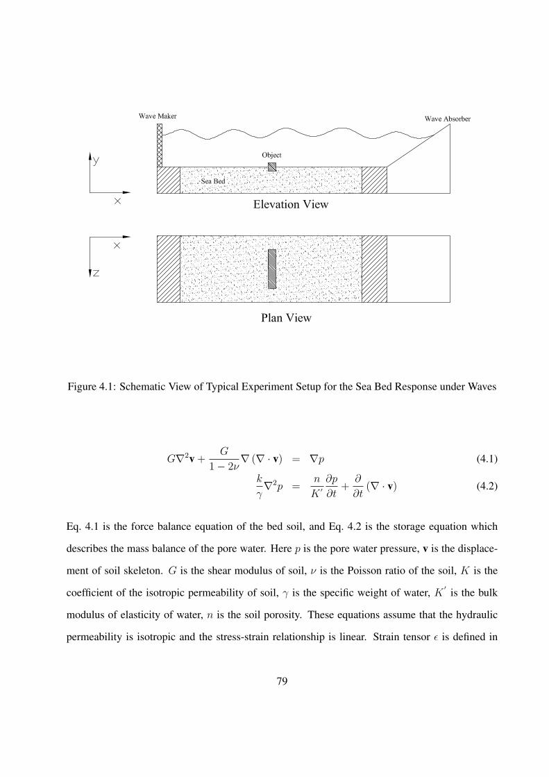
Figure 4.1: Schematic View of Typical Experiment Setup for the Sea Bed Response under Waves
G∇2v +G
1− 2ν∇ (∇ · v) = ∇p (4.1)
k
γ∇2p =
n
K ′∂p
∂t+
∂
∂t(∇ · v) (4.2)
Eq. 4.1 is the force balance equation of the bed soil, and Eq. 4.2 is the storage equation which
describes the mass balance of the pore water. Here p is the pore water pressure, v is the displace-
ment of soil skeleton. G is the shear modulus of soil, ν is the Poisson ratio of the soil, K is the
coefficient of the isotropic permeability of soil, γ is the specific weight of water, K′ is the bulk
modulus of elasticity of water, n is the soil porosity. These equations assume that the hydraulic
permeability is isotropic and the stress-strain relationship is linear. Strain tensor ε is defined in
79

terms of the displacement vector v as
ε =1
2
[∇v + (∇v)T
](4.3)
and the stress tensor σ is related to strain rate ε via
σ = σ′ − pI (4.4)
= 2Gε +
[2G
ν
1− 2νtr (ε)− p
]I (4.5)
where I is the unit tensor. tr(ε) is the trace of the tensor ε which is equal to ∇ · v. This equation
also says that the stress in soil is constituted by two parts:the effective stress σ′ supported by soil
skeleton and pore water pressure p. Here the stress-strain relationship is slightly different from
that of elastic solid. The only difference is that the pore pressure is included for the porous media.
Plane strain is also assumed here.
4.2.2 Navier-Stokes Equations
The governing equations for the wave part is the Navier-Stokes equations:
∇ · u = 0 (4.6)
∂ρu∂t
+∇ · (ρuu)−∇ · (µS) = −∇p + ρg + σK∇α
|∇α| (4.7)
where u is the velocity vector field, p is the pressure field, α is the volume fraction function for the
two fluids defined by
α =
0 volume occupied by air
1 volume occupied by water(4.8)
S is the strain rate tensor defined by S = 12
[∇u + (∇u)T]. σ is surface tension, K is the surface
curvature. Surface tension is not so important in current problem but it’s included for complete-
80

ness. The density ρ and viscosity µ in the domain is given by
ρ = αρ1 + (1− α)ρ2 (4.9)
µ = αµ1 + (1− α)µ2 (4.10)
Volume fraction α is transported by the fluid velocity field. The equation for the volume
fraction scalar α is∂α
∂t+∇ · (uα) = 0 (4.11)
Numerical diffusion will spread out the sharp interface between water and air. An compressive
interface capturing scheme is used to resharpen the interface. The details of the present free surface
modeling can be found in Ubbink and Issa (1999).
4.2.3 Turbulence k- ε Model
Equations in wave part are closed by conventional k- ε model (Lauder and Spalding 1973; Rodi
1993).
µt = Cµρk2
ε(4.12)
∂k
∂t+∇ · (uk) =
1
ρ∇(
µt
σk
∇k) + 2µt
ρ|∇u|2 − ε (4.13)
∂ε
∂t+∇ · (uε) =
1
ρ∇(
µt
σε
∇ε) + 2C1µt
ρ|∇u|2 ε
k− C2
ε2
k(4.14)
where µt is turbulence eddy viscosity, k is turbulence kinetic energy and ε is turbulence energy
dissipation rate. The constants appear in Eqs. (4.12), (4.13) and (4.14) take the values given in
Table 3.1.
81

4.3 Numerical Simulation Schemes and Procedures
The code used in this research is the open source numerical library (OpenCFD 2006). It’s freely
available through internet. OpenFOAM is primarily designed for problems in continuum mechan-
ics. It uses the tensorial approach and object oriented techniques (Weller et al. 1998). OpenFOAM
provides a fundamental platform to write new solvers for different problems as long as the prob-
lem can be written in tensorial partial differential equation forms. In this research, the flow field is
solved by the adaption of the original turbulence solver for incompressible fluid in the code. The
consolidation equation solver is newly added. The core of this code is the finite volume discretiza-
tion of the governing equations. Almost all kinds of differential operators possible in a partial
differential equation, such as temporal derivative, divergence, laplacian operator, curl, etc, can be
discretized in the code. The finite volume details of the code can be found in Jasak (1996). One
application of OpenFOAM in stress analysis can be found in Jasak and Weller (2000). Next several
sections briefly introduces the numerical schemes used in the coupled solvers.
4.3.1 Numerical Scheme for Foundation Part
Finite element method is usually used to solve the Biot equations of soil consolidation (Lewis and
Schrefler 1998) and to do other stress analysis. But finite volume method is becoming popular
because of its flexibility to deal with complex domain. In this chapter, FVM is used to solve
the consolidation equations. Comparing the Biot consolidation equations with the Navier-Stokes
equations shows they are very similar. Both equations couple two quantities (pore pressure and
displacement for consolidation, pressure and velocity for fluid) and both equations describes the
mass balance and force balance. Inspired by these similarities, a new scheme is proposed to solve
consolidation equations on an iterative basis. This iterative procedure is similar to the SIMPLE
and PISO schemes for Navier-Stokes equations. A segregated approach is used to solve the couple
consolidation equation which means components of the displacement vector and pore pressure are
solved separately. At each time step, storage equation (Eq. 4.2) is rearranged into implicit and
82
explicit parts and is solved first according to
− n
K ′∂p
∂t+
k
γ∇2p
︸ ︷︷ ︸implicit
=∂
∂t(∇ · v)
︸ ︷︷ ︸explicit
(4.15)
where the displacement v in the explicit part is from previous iteration or initial condition. Then
the force balance equation (Eq. 4.1) is solved. In order to get higher efficiency of the segregated
solver and to increase the convergence radius, a decomposition and a rearrangement of Eq. 4.1 is
carried out similar to Jasak and Weller (2000). The terms in the equation are also split into implicit
part and explicit part. The aim is to achieve maximum implicity. Assuming G and ν are constant,
using the fact that
∇ (∇ · v) = ∇ · (I∇ · v) = ∇ · (Itr (∇v)) (4.16)
the force balance equation (Eq. 4.1) can be written as
G∇2v +G
1− 2ν∇2v
︸ ︷︷ ︸implicit
= ∇p−∇ ·(
G
1− 2νItr (∇v)− G
1− 2ν∇v
)
︸ ︷︷ ︸explicit
(4.17)
Eq. 4.17 is solved for each component of vector v and the resulting v is used to solve storage
equation again. This inner coupling is looped until desired convergence tolerance is achieved.
4.3.2 Numerical Scheme for Fluid Part
The numerical solution for Navier-Stokes equation of incompressible fluid flow imposes two main
problems (Jasak 1996): the nonlinearity of momentum equation and the pressure-velocity cou-
pling. For the first problem, two common methods can be used to deal with it. The first is to solve
a nonlinear algebra systems after the discretization. This will need a lot of computational effort.
The other is to linearize the convection term in the momentum equation by using the fluid velocity
in old time steps which satisfies the divergence-free condition. The latter method is used in this
research. For pressure-velocity coupling, many schemes exist, such as SIMPLE (Patankar 1981)
83
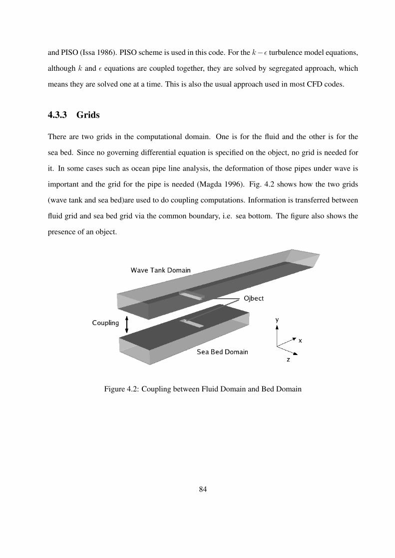
and PISO (Issa 1986). PISO scheme is used in this code. For the k−ε turbulence model equations,
although k and ε equations are coupled together, they are solved by segregated approach, which
means they are solved one at a time. This is also the usual approach used in most CFD codes.
4.3.3 Grids
There are two grids in the computational domain. One is for the fluid and the other is for the
sea bed. Since no governing differential equation is specified on the object, no grid is needed for
it. In some cases such as ocean pipe line analysis, the deformation of those pipes under wave is
important and the grid for the pipe is needed (Magda 1996). Fig. 4.2 shows how the two grids
(wave tank and sea bed)are used to do coupling computations. Information is transferred between
fluid grid and sea bed grid via the common boundary, i.e. sea bottom. The figure also shows the
presence of an object.
Figure 4.2: Coupling between Fluid Domain and Bed Domain
84
4.3.4 Boundary Conditions
Boundary Conditions for the Sea Bed Domain
In this chapter, only finite soil depth is considered for the sea bed domain because it’s the case for
most of the physical experiments. Infinite soil depth case can be achieved by extending the sea
bed downward until the numerical result won’t change anymore. The boundary conditions for the
sea bed domain is very similar to Magda (1996) and Jeng and Lin (1999). At the bottom of the sea
bed, zero displacements and zero vertical flow are specified, i.e.
v = 0 (4.18)
∂p
∂n= 0 (4.19)
where n is the surface normal direction vector.
At the top of sea bed (i.e. the common boundary between two domains), the fluid shear stress
is neglected and the pore water pressure is equal to water wave pressure on the bed. This pressure
value comes from the fluid solver. For the displacement on this surface, it’s more complicated.
Since the pore water pressure is set to be the wave pressure, the effective normal stress σ′yy on the
this boundary is zero. This gives the boundary condition of Neumann type (traction boundary) for
displacement (Demirdzic et al. 1994; Jasak and Weller 2000)
n · ∇v =t− n ·
[µ (∇v)T − (µ + λ)∇v
]− λn∇ · v
2µ + λ(4.20)
where t is the traction stress on the bed which equals zero for the free bed surface in this case.
On the surfaces of object, it’s assumed that no water can flow through. So zero pressure
gradient as in Eq. 4.19 applies. For the displacement on the object, the object sides and bottom are
considered separately. For the object sides, it’s assumed that the sides are smooth and the soil can
slip on the surface. The normal displacement component on the sides are set to zero. For the object
85

bottom, the traction boundary condition (Eq. 4.20) is specified. The traction on the bottom is from
the simple force balance of the object (see Fig. 4.3). The forces on the object are flow drag Fdrag,
flow lift Flift, gravity mg and bottom supporting force. The friction force on the object sides are
neglected. This is reasonable because the sand on the sides of the object can be assumed loosely
back filled in experiment. The flow drag and lift are calculated at each time step from the flow
solver. So the Neumann type condition in Eq. 4.20 is applied with traction t from force balance of
the object. This assumption is valid if the object is rigid body and will not move. It will be violated
if the object is moving under wave force.
Figure 4.3: Force Balance of the Object
86

Boundary Conditions for Fluid Domain
The wave in the physical experiment is usually generated by a piston type wave maker and at
the end of the wave tank, there is a wave absorber to eliminate the wave reflection. In numerical
simulation, the wave can be generated generally by two approach: moving mesh (Aliabadi et al.
2003) and wave boundary condition (Mayer et al. 1998). For moving mesh approach, the piston
movement is simulated by moving the boundary of the computational domain. For wave boundary
condition approach, the mesh is fixed but boundary condition on the piston part is given by wave
theory. The second approach is adopted in this chapter. A time varying velocity profile is imposed
at the piston boundary to generate the waves
~U = fr(t)[~U(y)sin(ωt + θ)
](4.21)
where ~U is the velocity vector at the boundary, ω is the wave frequency, θ is the phase. ~U(y) is
imposed by the type of the piston. fr(t) is the ”ramp” function to start up the piston. fr(t) has the
form
fr(t) =
tT− 1
πsin
(π t
T
)for 0 < t < T
1 for t > T(4.22)
where T is the wave period.
The wave absorber is simulated using a damping zone (or sponge layer). In this damping zone,
extra fluid viscosity is added to the momentum equation to dissipate the fluid dynamic energy.
In numerical test cases, in order to eliminate the introduced artificial effect, the damping zone is
extended far downstream. That’s the reason that the wave tank domain used in this chapter will
be longer than the sea bed domain. An alternative method by modifying the water depth and fluid
velocity in the damping zone can be found in Mayer et al. (1998).
At the piston, pressure is set to be zero normal gradient to be consistent with velocity condition.
Turbulence quantities such as k and ε are set as zero normal gradient at the piston wall. The
87

condition at the wave tank outlet is chosen as zero gradient for all quantities except pressure which
is specified as hydrostatic (i.e., the dynamic pressure is zero). The top boundary of the fluid
domain is atmosphere. The dynamic pressure is set to zero as the outlet and the velocity is set
to zero. Other quantities are set to zero normal gradient. At the object’s surfaces or flume walls,
it is assumed to be hydraulically smooth. No-slip condition is set for velocity with zero normal
gradient for pressure. Other quantities such as k and ε are also set as zero normal gradient.
4.3.5 Simulation Process
In order to study the effect of waves, base state of pore pressure and displacement without wave
is obtained by doing the computation for a period of time with the wave maker shut off. This
resembles the fact that in the experiment, the bed soil is already in the equilibrium state before
the wave maker is started. After that, the wave maker boundary condition is switched on and
waves are generated. Base stable pore pressure and displacement is subtracted from the result to
investigate the effect of waves. The main application of current numerical model is the study of
liquefaction potential. When the pore water pressure is so excessive that the effective stress in soil
is zero or negative, the soil is in the state of liquefaction (Jeng 1996). For a flat bed, the criterion
for liquefaction isp
13(γs − γw) (1 + 2K0) y
≥ 1 (4.23)
where p is excessive pore pressure, γs and γw are unit weight of soil and water, K0 is the coefficient
of lateral earth pressure at rest which ranges from 0.4 to 1.0. y is the depth of the soil measured
downward from the bed. But for complicated computational domain, it is not easy to calculate the
effective soil gravity force at each point in the bed. In this chapter, the dimensionless excessive
pore water pressure (non-dimensionized by p0 = ρgH0, where H0 is the wave height) is used as
an indicator for the liquefaction potential.
At each time step, the fluid field is first solved and the pressure on the sea bed is mapped to the
bed domain. Based on the pressure from fluid solver, the Biot consolidation equations are solved.
88

This process continues until wave period averaged pore pressure and displacement reach steady
state or the specified computation time is reached.
4.4 Model Verification and Applications
4.4.1 Verification of FVM Solver for Biot Consolidation Equations
In order to verify the Biot equation solver in the numerical model, a test case which is similar
to that of Jeng and Lin (1999) is carried out. Fig. 4.4 is the schematic view of the test case. The
details of the test case can be found in Jeng and Lin (1999) and the analytical solution can be found
in Jeng and Hsu (1996). In this test case, uniform sea bed is under the progressive wave. The bed
soil depth h = 1m and the wave pressure amplitude pb = 2000N/m2. The wave number k = π
and wave frequency ω = 2π.
Figure 4.4: Numerical Test of Sea Bed Response
The numerical result of excessive pore pressure at each depth of the soil versus kx − ωt is
plotted in Fig. 4.5. The analytical solution is also plotted. The difference between numerical result
89

and analytical solution is so small that they are almost identical to each other. From the figure,
the excessive pore pressure diffuses with the increase of depth which is as expect. For flat bed,
top layers of soil are most vulnerable to storm waves and failure of foundation due to liquefaction
always happens in these layers.
-0.1 0.0 0.1 0.2 0.3 0.4 0.5 0.6 0.7 0.8 0.9 1.0 1.1-1.2
-1.0
-0.8
-0.6
-0.4
-0.2
0.0
0.2
0.4
0.6
0.8
1.0
1.2
y=0 y=0.25h
y=0.90h
p/p
b
kx-ωt
Numerical
Analytical
-0.2 -0.1 0.0 0.1 0.2 0.3 0.4 0.5 0.6 0.7 0.8 0.9 1.0 1.1-1.2
-1.0
-0.8
-0.6
-0.4
-0.2
0.0
0.2
0.4
0.6
0.8
1.0
1.2
p/p
bkx-ωt
Numerical
Analytical
-0.1 0.0 0.1 0.2 0.3 0.4 0.5 0.6 0.7 0.8 0.9 1.0 1.1-1.2
-1.0
-0.8
-0.6
-0.4
-0.2
0.0
0.2
0.4
0.6
0.8
1.0
1.2
p/p
b
kx-ωt
Numerical
Analytical
-0.1 0.0 0.1 0.2 0.3 0.4 0.5 0.6 0.7 0.8 0.9 1.0 1.1-1.2
-1.0
-0.8
-0.6
-0.4
-0.2
0.0
0.2
0.4
0.6
0.8
1.0
1.2 y=0.99h
p/p
b
kx-ωt
Numerical
Analytical
Figure 4.5: Pore Pressure Comparison between Numerical and Analytical Solution
Fig. 4.6 shows the numerical results of the test case. Fig. 4.6(a) shows the pore water pressure
and Fig. 4.6(b) shows the displacement magnitude. From the figures, it’s clear that under wave
crest the pressure on the bed is increased and the soil is compressed. Under wave trough, it’s
just the opposite. The displacement vector field in Fig. 4.7 demonstrates this pattern even more
clearly. The geometry in this figure is distorted by 1E + 4 times the displacement to show elastic
deformation.
90
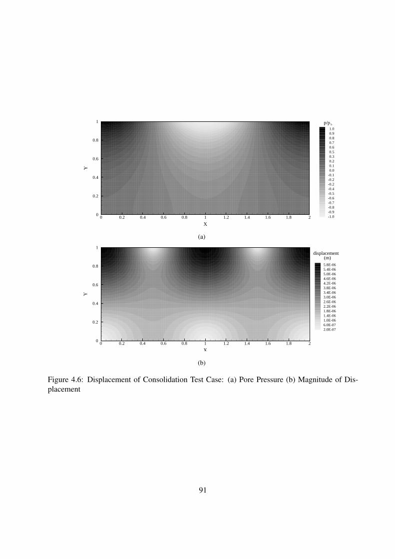
X
Y
0 0.2 0.4 0.6 0.8 1 1.2 1.4 1.6 1.8 20
0.2
0.4
0.6
0.8
1
1.00.90.80.70.60.50.30.20.10.0
-0.1-0.2-0.2-0.4-0.5-0.6-0.7-0.8-0.9-1.0
p/pb
(a)
X
Y
0 0.2 0.4 0.6 0.8 1 1.2 1.4 1.6 1.8 20
0.2
0.4
0.6
0.8
1
5.8E-065.4E-065.0E-064.6E-064.2E-063.8E-063.4E-063.0E-062.6E-062.2E-061.8E-061.4E-061.0E-066.0E-072.0E-07
displacement(m)
(b)
Figure 4.6: Displacement of Consolidation Test Case: (a) Pore Pressure (b) Magnitude of Dis-placement
91
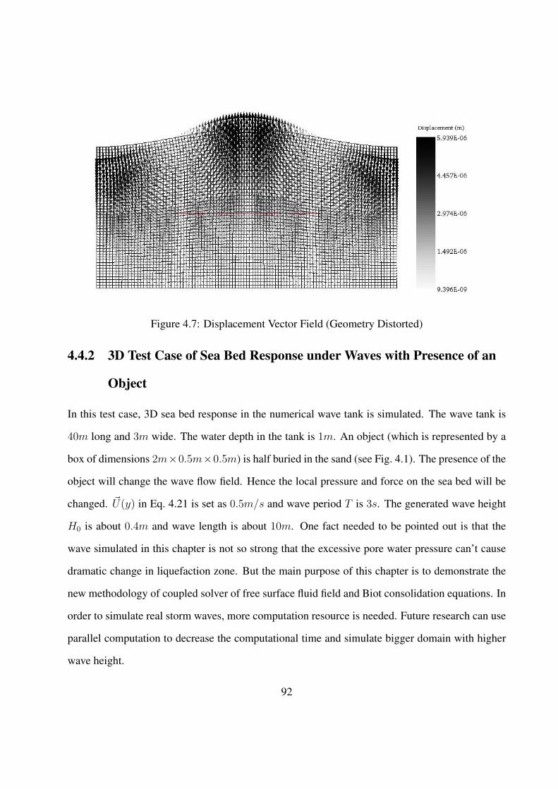
Figure 4.7: Displacement Vector Field (Geometry Distorted)
4.4.2 3D Test Case of Sea Bed Response under Waves with Presence of an
Object
In this test case, 3D sea bed response in the numerical wave tank is simulated. The wave tank is
40m long and 3m wide. The water depth in the tank is 1m. An object (which is represented by a
box of dimensions 2m×0.5m×0.5m) is half buried in the sand (see Fig. 4.1). The presence of the
object will change the wave flow field. Hence the local pressure and force on the sea bed will be
changed. ~U(y) in Eq. 4.21 is set as 0.5m/s and wave period T is 3s. The generated wave height
H0 is about 0.4m and wave length is about 10m. One fact needed to be pointed out is that the
wave simulated in this chapter is not so strong that the excessive pore water pressure can’t cause
dramatic change in liquefaction zone. But the main purpose of this chapter is to demonstrate the
new methodology of coupled solver of free surface fluid field and Biot consolidation equations. In
order to simulate real storm waves, more computation resource is needed. Future research can use
parallel computation to decrease the computational time and simulate bigger domain with higher
wave height.
92

Fig. 4.8 shows the fluid force components and magnitude on the object. The forces on the ob-
ject undergo periodical changes. The most significant components are in the streamwise direction
and vertical direction which is as expected. The spanwise fluid force is very small comparing with
the other two. Second mode effect can also be seen in the figure but is not significant. This could
be caused by the wave reflection from the object or the wave tank end. The forces are used to
calculate the traction boundary condition on the object bottom.
0 2 4 6 8 10 12 14 16 18 20 22 24 26 28 30-600
-400
-200
0
200
400
600
800
1000
1200
1400
1600
Forc
e (N
)
t (s)
X-direction
0 2 4 6 8 10 12 14 16 18 20 22 24 26 28 30-4500
-4000
-3500
-3000
-2500
-2000
-1500
-1000
Forc
e (N
)
t (s)
Y-direction
0 2 4 6 8 10 12 14 16 18 20 22 24 26 28 30-8
-6
-4
-2
0
2
4
6
8
Forc
e (N
)
t (s)
Z-direction
0 2 4 6 8 10 12 14 16 18 20 22 24 26 28 301000
1500
2000
2500
3000
3500
4000
4500
Forc
e (N
)
t (s)
Magnitude
Figure 4.8: Object Force History
In Fig. 4.9, the free surface of waves in one typical period is plotted. The wave height relative
to the water depth can also be seen. Fig. 4.10 shows the iso-surface of the dimensionless instan-
taneous excessive pore pressure inside the sea bed. With the propagation of the wave, the sea bed
pressure response also moves forward accordingly.
93

(a)
(b)
Figure 4.9: Free Surface of Waves in One Typical Period: (a) t = t0 +T
4(b) t = t0 +
T
2(c)
t = t0 +3T
4(d) t = t0 + T
94

(c)
(d)
Figure 4.9: Free Surface of Waves in One Typical Period (Cont’d): (a) t = t0 +T
4(b) t = t0 +
T
2
(c) t = t0 +3T
4(d) t = t0 + T
95

(a)
(b)
Figure 4.10: Dimensionless Excessive Pore Pressure under Waves in One Typical Period : (a)
t = t0 +T
4(b) t = t0 +
T
2(c) t = t0 +
3T
4(d) t = t0 + T
96
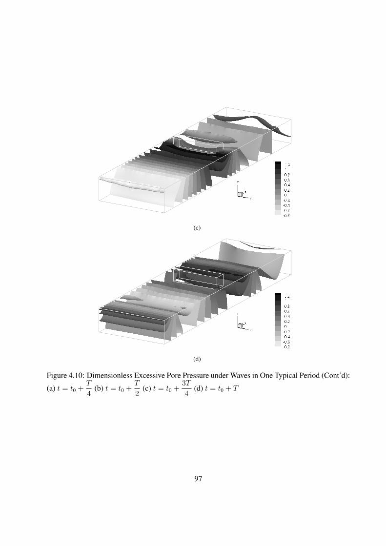
(c)
(d)
Figure 4.10: Dimensionless Excessive Pore Pressure under Waves in One Typical Period (Cont’d):
(a) t = t0 +T
4(b) t = t0 +
T
2(c) t = t0 +
3T
4(d) t = t0 + T
97

Fig. 4.11 is the contour plot of non-dimensionized excessive pore pressure under the instan-
taneous flow field (t = t0 + 3T4
) in Fig. 4.9(c). The reason to plot for this time point is that the
wave crest is almost on top of the object and it’s considered to be the most possible time for the
momentary liquefaction to happen. From the figures, it’s clear the pressure distribution is disturbed
by the half buried object. At this very moment, the excessive pore pressure in front of the object
is very high and the liquefaction potential in this area and under the object is amplified. From the
slice view, the excessive pore pressure beneath the object is also at the peak value. This is caused
by two facts. One is that the wave crest in just above the object. The other is that the fluid forces
on the object are also at maximum values.
4.5 Discussion
4.5.1 Soil Constitutive Model Effects
For geotechnical problems, a realistic stress-strain constitutive relationship is one of the most
important things for the ability of the numerical model to reproduce the reality situations. Herein,
the simple linear isotropic elastic model is used to describe the soil skeleton. More advanced
and accurate constitutive models (such as variable elasticity, elasto-plastic model and visco-plastic
model, etc.) can be easily incorporated in the current numerical code. Anisotropic effect can also
easily come into the model since the code is based on the tensorial description of the equations and
anisotropic tensors can be included inside the differential operators.
4.5.2 Residual Liquefaction Effects
Only momentary liquefaction is model in this chapter since it is simple and easy. Liquefaction is
an complicated physical process which is still not well understood today. Liquefaction is generally
caused by two main mechanisms: momentary liquefaction and residual liquefaction (Sumer and
Fredsøe 2002). Residual liquefaction is more complicated than momentary liquefaction because
98
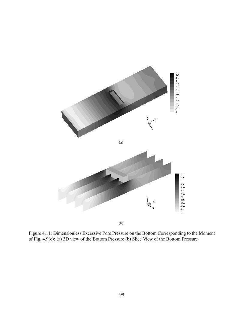
(a)
(b)
Figure 4.11: Dimensionless Excessive Pore Pressure on the Bottom Corresponding to the Momentof Fig. 4.9(c): (a) 3D view of the Bottom Pressure (b) Slice View of the Bottom Pressure
99
the pore pressure builds up with time. Some simplified models existing for the residual liquefaction
add a source term to the governing equation of pore pressure. This can also easily be incorporated
into current model. Further research is needed to carefully verify the parameters and to what
happens after the liquefaction.
4.5.3 Bed Morphodynamics and Object Movement
In the wave-seabed-object system, another process, sediment transport, is also very important
and is closely related the flow field and bed soil. Flow field change around the object causes
scour and deposition of the sediment. Sediment movement will change the sea bed elevation
and consequently affect the flow field. This sea bed change also will change the domain of the
consolidation and change the pore pressure distribution. Scour is one of the main reasons of
foundation failure in ocean and river engineering. Sediment transport together with the other
processes modeled in this chapter forms an even bigger coupled system. Sediment transport and
morphodynamic models should be included in the future.
The object is assumed to be at fixed position during the computation. This is not always true
since when the liquefaction occurs, the soil can’t support the object any more and the object will
move. Even without liquefaction, the object could rotate or slide under the influence of fluid
force. All these make the problem extremely complicated and it’s impossible to include all factors
into the numerical model. But by fixing the object in one position, it is possible to investigate
the possibility of liquefaction and analyze the dynamics of the system. This could be useful for
engineers to design structure and foundations to prevent damage under extreme conditions.
4.6 Conclusion
The numerical model in this chapter can solve the coupling problem between waves, object (struc-
ture) and sea bed response. Sea bed response under wave is one of the keys to the understanding of
liquefaction. The wave induced shear stress and pore pressure in the soil is governed by Biot con-
100

solidation equation. Free surface is modeled by Volume of Fluid (VOF) method and water wave is
generated by numerical wave maker boundary condition. Instead of using finite element method
to do stress analysis inside the bed material which is the traditional method used in geotechniques,
an iterative numerical scheme is proposed to solve Biot consolidation equation using finite volume
method. The new scheme shows fast convergence rate and high accuracy. The coupling between
water wave and sea bed is through pressure and stress condition on common boundaries. Two
numerical tests of the proposed scheme is carried out. First numerical case tests the consolida-
tion solver part of the numerical model. Good agreement with analytical results is obtained. The
second case is a 3D test to study the interaction between wave, sea bed and object. A box is half
buried in the wave tank. More complicated real geometry can be simulated as well. From the result
excessive pore pressure of the sea bed, liquefaction potential can be analyzed. Only momentary
liquefaction can be studied using current model. For residual liquefaction, the modified Biot con-
solidation equation should be solved. The model proposed in this chapter can be used to guide the
design of under water structures and foundations.
101

Chapter 5
Models for the Residual Pore WaterBuildup Process
5.1 Introduction
Liquefaction can cause enormous damage to infrastructures, and there has been great interest in the
geotechnical profession to study the liquefaction due to earthquakes and general cyclic loadings.
The most cited example of liquefaction damage due to the earthquake is the Alaska and Niigata
earthquake in 1964 where buildings tilted. During an earthquake, shear waves are propagated
upwards in the sediment deposit from the earthquake center to the surface. During an ocean storm,
the water waves will induce cyclic shear stress on the bottom of the seabed. This cyclic shear stress
will also lead to the buildup of excessive pore pressure in the same way as during an earthquake.
Another aspect for an ocean storm is when structures interact with the water waves and the seabed,
lateral forces and overturning momentum will be exerted on the structure. The forces and the
momentum will change direction during one wave period. These facts will cause the foundation
soil to experience cyclic stresses in both horizontal and vertical directions (Taiebat 1999).
In general, liquefaction is a term used to describe the behavior of loose saturated cohesionless
soils, i.e. loose sands, which go from a solid state to a heavy liquid, or reach a liquefied state as
a consequence of increasing pore water pressures, and thus decreasing effective stress. In Seed
(1976), liquefaction is defined as a condition where soil deforms continuously with low residual
strength or without strength. Liquefaction is more likely to occur in loose to moderate granular
∗This chapter, as a manuscript, is in preparation for possible publication in Journal of Engineering Mechanics,ASCE
102
soils with poor drainage. Deposits most susceptible to liquefaction are young sands and silts of
similar grain size (well-sorted), in beds at least several feet thick, and saturated with water. Such
deposits are often found along river beds, beaches, and dunes. Some examples of liquefaction
include quicksand, quick clay, fluid mud, and earthquake liquefaction (Wikipedia 2007). Although
liquefaction can happen under both static and cyclic loadings, this chapter limits the study to the
case of liquefaction due the cyclic loadings.
The interest in liquefaction is growing because it is important for geotechnical engineers to
design onshore/offshore foundations and structures. Liquefaction is one of the main mechanisms
which dominates the interaction between water waves, sea bed, and structures. Due to liquefaction,
the supporting foundations will loose their strength and the supported structures (such as oil pipe
lines) will sink or float and hence cause damage. Experimental work (Sakai et al. 1994; Sumer
et al. 1999) and numerical simulations (Magda 1996; Jeng and Lin 1999; Gao et al. 2003; Liu
and Garcıa 2006b; Cardenas and Wilson 2007) have been done to understand this complicated
process. Analytical models which describe the sea bed response under waves have been developed
for many years. Yamamoto (1977) treated the wave-induced sea bed response analytically based
on the three-dimensional Biot consolidation theory (Biot 1941). Closed form of the analytical
solutions are given. One conclusion from the paper is that the bed response is strongly dependent
on the permeability and the stiffness ratio G/K′ , where G is the shear modulus and K
′ is the
apparent bulk modulus of elasticity of water.
Mei and Foda (1981) treated the porous elastic medium using Biot’s linearized theory, which
can be seen as a special case of the mixture theory. For sufficiently high frequency waves, the area
near the water-soil interface can be divided into a boundary layer of Stokes’ type and an outside
layer. In the outside layer, fluid and the solid skeleton move together according to the laws of the
classical elasticity theory for a single phase. Based on this division, the governing equations can
be simplified and analytical solutions are proposed.
In Jeng and Hsu (1996), a closed-form analytical solution is developed for the wave-induced
pore pressure, soil displacements, and effective stresses in an elastic sea-bed subject to a system of
103

two intersecting waves. Although the solution is for the finite depth soil, it can be reduced to the
conditions for soil of infinite thickness. The solution can also be extended to the limiting cases of
two-dimensional progressive and standing waves for soil of finite thickness. The authors compared
their analytical solutions with numerical results and the solutions from Yamamoto (1977) and Mei
and Foda (1981). The proposed solutions are found in complete agreement with the results of
Yamamoto (1977) for both fine sand and coarse sand. The solutions also agree with those of Mei
and Foda (1981) for the fine sand while deviation is observed for coarse sand. In Jeng et al. (2007),
a new approximation for the pore water pressure buildup in marine sediments is proposed which
will be discussed in detail in this chapter.
Cheng et al. (2001) corrected some errors contained in the analytical solution for wave-induced
pore pressure accumulation in McDougal et al. (1989) and gave the revised solution in a more
general form. The authors studied the behavior of the solution under different soil conditions.
For deep soil, the solution is sensitive to the soil shear stress in the top thin layer of the soil. In
contrast, for shallow and finite depth soil, the solution is sensitive to shear stress in the thin layer of
soil near the impermeable base. It is also found that a small error in the soil shear stress can lead to
a large error in the accumulated pore pressure. Sensitivity analysis is also done to investigate the
relationships between the accuracy of the pore pressure accumulation and the accuracy of the soil
shear stress. In that paper, the simplified Biot consolidation equations are also solved numerically.
Both analytical and numerical examples are given to validate the error estimation method proposed
in that paper.
Most analytical models assume the soil to be an isotropic medium while natural soils always
display some degree of anisotropy. The effects of soil anisotropy will have great effect on the
sea bed response. They are revealed as the anisotropy of the soil Young’s modulus, Poisson’s
ratio, and permeability. Analytical solutions which consider the soil anisotropy are complicated
(Gatmiri 1992; Jeng 1997). Yuhi and Ishida (2002) gave simplified analytical solutions for the
wave-induced response of a cross-anisotropic seabed of infinite thickness for both slightly and
fully saturated conditions.
104
The literature mentioned above for liquefaction is almost all based on the linear theory of Biot
consolidation. There are other theories proposed to explain the phenomenon of liquefaction. Foda
et al. (1993) considered the rheological properties of marine sediment and incorporated them into
potential flow equations for both water layer and the fluidized mud layer. The fluidization depth of
the sediment is solved as a function of the imposed wave height.
Aside from analytical models, numerical models, especially from computational geomechan-
ics, have also been developed to predict the liquefaction in the soil (Zienkiewicz et al. 1999). The
poro-elastic model is the simplest constitutive relationship, and it is used in most analytical mod-
els. The elasto-plastic model is more popular in computational geomechanics, and it gives results
which are closer to the experiment. Although it is easier to implement different constitutive re-
lationships, the non-linearity associated with these relationships increases the computational cost
tremendously.
Taiebat (1999) developed a three-dimensional elasto-plastic finite element model for the lique-
faction problem of offshore foundations. By representing the variables of an axis-symmetric body
as a discrete Fourier series, the three-dimensional problem is reduced to several small problems
and therefore the computational cost is also reduced. This author proposed a new procedure for the
liquefaction analysis of offshore foundations subjected to storm loadings. The numerical model is
used to evaluate the liquefaction problem of Ekofisk tank which is constructed in North Sea.
Dunn et al. (2006) used the finite element model, DIANA-SWANDYNE II (Chan 1995) to
study the wave-induced liquefaction around offshore structures. It is a two-dimensional model with
the plane strain assumption. It solves the fully coupled Biot dynamic equation for both drained and
undrained conditions. Different constitutive relationships are implemented in the model. Among
many other interesting results, the authors found that the excessive pore pressure builds up more
quickly around the structure and the boundary conditions at the structure have a great effect on the
results.
Although many numerical models have been developed to solve sea bed response under waves,
most of them just use the wave pressure on the water-bed interface by wave theory. This is valid
105

when there is only water wave and sea bed interaction. But when there is extra object in the
system (such as pile, semi-buried foundation, etc.), the water flow around the object will be highly
three-dimensional and it is not easy to get an analytical solution from wave theory. Wave, sea
bed, and object form a large coupled system. Multi-physics numerical models have been widely
used to solve these coupled systems. The approach in these models is to solve different governing
equations on different domains and to couple the system through common boundaries or other
ways. Three-dimensional CFD models can be used to predict the free surface wave field and the
results can be used as boundary condition for the sea bed governing equations (Liu and Garcıa
2006b; 2007a).
The structure of this chapter is as follows. The governing equations for the consolidation of
poro-elastic soil will be introduced. Source term, which is responsible for the excessive pore
pressure generation, is added to the governing equations. Under some simplifications, the new
equations system for the period-averaged pore pressure has analytical solutions. The analytical
solutions of the sea bed pore pressure due to the progressive waves found in the literature are
summarized. For deep sea bed, the behavior of the pore pressure is estimated using an asymptotic
method. Numerical simulations which include the source term effect are carried out, and the results
are compared with experiment and analytical solutions. At the end, a tentative effort is made
to simulate the phase-resolved residual pore water pressure buildup process using the numerical
model introduced in Chapter 4 with an extra source term from the current chapter.
5.2 Governing Equations
5.2.1 Three-Dimensional Biot Consolidation Equations
Governing equations for the poro-elastic seabed two-phase media is the Biot consolidation equa-
tion (Biot 1941):
106

G∇2v +G
1− 2ν∇ (∇ · v) = ∇p (5.1)
k
γ∇2p =
n
K ′∂p
∂t+
∂
∂t(∇ · v) (5.2)
Eq. 5.1 is the force balance equation of the bed soil, and Eq. 5.2 is the storage equation which de-
scribes the mass balance of the pore water. Here p is the pore water pressure, v is the displacement
of soil skeleton. G is the shear modulus of soil, ν is the Poisson ratio of the soil, K is the coeffi-
cient of the isotropic permeability of soil, γ is the specific weight of water, β is the compressibility
of pore water, and n is the soil porosity. These equations assume that the hydraulic permeability
is isotropic and the stress-strain relationship is linear. Strain tensor ε is defined in terms of the
displacement vector v as
ε =1
2
[∇v + (∇v)T
](5.3)
and the stress tensor σ is related to strain rate ε via
σ = σ′ − pI (5.4)
= 2Gε +
[2G
ν
1− 2νtr (ε)− p
]I (5.5)
where I is the unit tensor. tr(ε) is the trace of the tensor ε which is equal to ∇ · v. This equation
also states that the stress in soil is constituted by two parts: the effective stress σ′ supported by
soil skeleton and the pore water pressure p. Here the stress-strain relationship is slightly different
from that of an elastic solid. The only difference is that the pore pressure is included for the porous
media. Plane strain is also assumed here.
107

5.2.2 One-Dimensional Period-Average Pore Pressure Equations
McDougal et al. (1989) derived the simplified equation governing the buildup of pore water pres-
sure. Assuming that the process is only one-dimensional in the vertical z direction, i.e., the varia-
tions with respect to other directions are negligible, then Eq. 5.1 can be written as
G2− 2ν
1− 2ν
∂2w
∂z2=
∂p
∂z(5.6)
and Eq. 5.2 becomesk
γ
∂2p
∂z2=
n
K ′∂p
∂t+
∂2w
∂z∂t(5.7)
Taking the derivative of Eq. 5.6 with respect to t and Eq. 5.7 with respect to z, and then cross
eliminating the terms with w, the equations become
cv∂3p
∂z3=
∂2p
∂z∂t(5.8)
where cv is the coefficient of consolidation which has the form of
cv =Gk
γ
2− 2ν
(1− 2ν) + (2− 2ν) nGK′
(5.9)
Integrating Eq. 5.8 with respect to z gives
∂p
∂t= cv
∂2p
∂z2+ c (5.10)
where c is a constant. Moving-averaging Eq. 5.10 gives the governing equation for the period-
averaged pore pressure∂p
∂t= cv
∂2p
∂z2+ f (5.11)
108

The period-averaged pore pressure is defined as
p =1
T
∫ t+T
t
pdt (5.12)
where T is the wave period. Eq. 5.11 is a diffusion equation with a source term f which is
the amount of pore water pressure generated per unit time and per unit volume. Although from
the derivation of the Eqs. 5.8 5.10 and 5.11, f should only be a function of time t, McDougal
et al. (1989) suggested that in general f can be considered to be a function of both time t and
space variable z. Careful examination of Eq. 5.11 reveals that the excessive pore water pressure is
generated through the source term f and spreads with sediment depth through the diffusion process
where cv plays the role of diffusion coefficient (Sumer and Fredsøe 2002).
In order to solve Eq. 5.11, the following boundary conditions and initial conditions are needed:
p(z, 0) = p(0, t) = 0 (5.13)
∂p(h, t)
∂z= 0 (5.14)
where h is the depth of the sediment. When the sediment is very deep, i.e., h → +∞, Eq. 5.14
still holds.
The source term f for the excessive pore water pressure generation comes from the cyclic shear
of the soil. It is important to know the normal and shear stresses in the soil due to waves beforehand
since most of the models for the source term f depend on the stress state of the soil. Analytical
solutions for wave-induced stresses in sea bed sediment have been developed by researchers (Ya-
mamoto et al. 1978; Madsen 1978; Okusa 1985; Jeng and Hsu 1996). In Jeng and Hsu (1996), the
amplitudes of the oscillatory pore water pressure and the shear stress for a saturated, isotropic sea
bed of finite thickness are given by
p0 =Pb
1− 2µ
[(1− 2µ)
(C2e
−kz − C4ekz
)+ (1− µ)
(δ2 − k2
) (C5e
−δz − C6eδz
)](5.15)
109
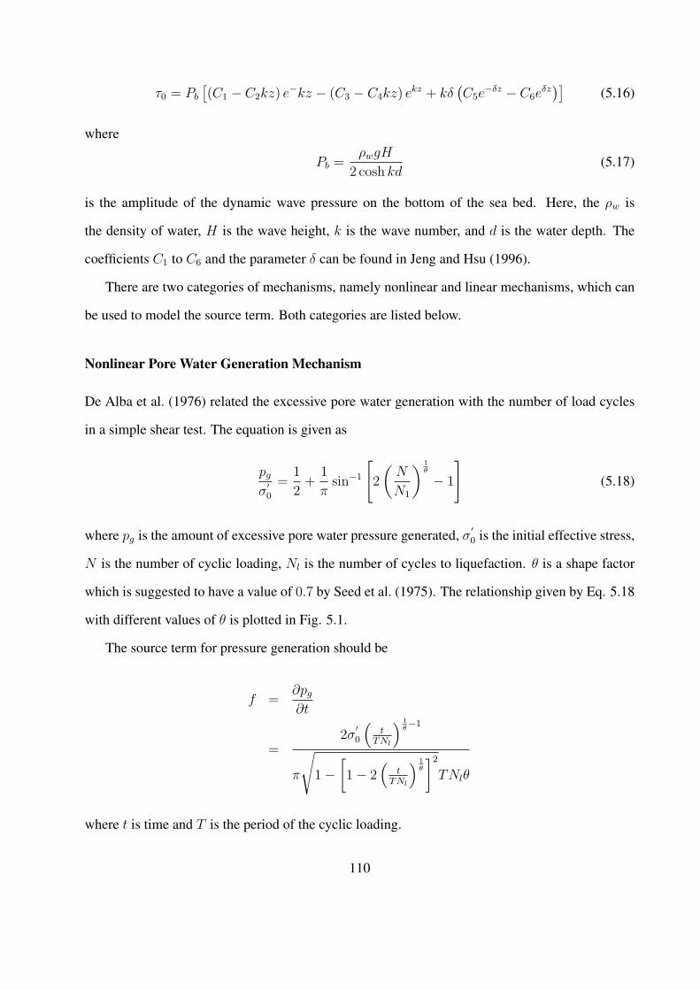
τ0 = Pb
[(C1 − C2kz) e−kz − (C3 − C4kz) ekz + kδ
(C5e
−δz − C6eδz
)](5.16)
where
Pb =ρwgH
2 cosh kd(5.17)
is the amplitude of the dynamic wave pressure on the bottom of the sea bed. Here, the ρw is
the density of water, H is the wave height, k is the wave number, and d is the water depth. The
coefficients C1 to C6 and the parameter δ can be found in Jeng and Hsu (1996).
There are two categories of mechanisms, namely nonlinear and linear mechanisms, which can
be used to model the source term. Both categories are listed below.
Nonlinear Pore Water Generation Mechanism
De Alba et al. (1976) related the excessive pore water generation with the number of load cycles
in a simple shear test. The equation is given as
pg
σ′0
=1
2+
1
πsin−1
[2
(N
N1
) 1θ
− 1
](5.18)
where pg is the amount of excessive pore water pressure generated, σ′0 is the initial effective stress,
N is the number of cyclic loading, Nl is the number of cycles to liquefaction. θ is a shape factor
which is suggested to have a value of 0.7 by Seed et al. (1975). The relationship given by Eq. 5.18
with different values of θ is plotted in Fig. 5.1.
The source term for pressure generation should be
f =∂pg
∂t
=2σ
′0
(t
TNl
) 1θ−1
π
√1−
[1− 2
(t
TNl
) 1θ
]2
TNlθ
where t is time and T is the period of the cyclic loading.
110
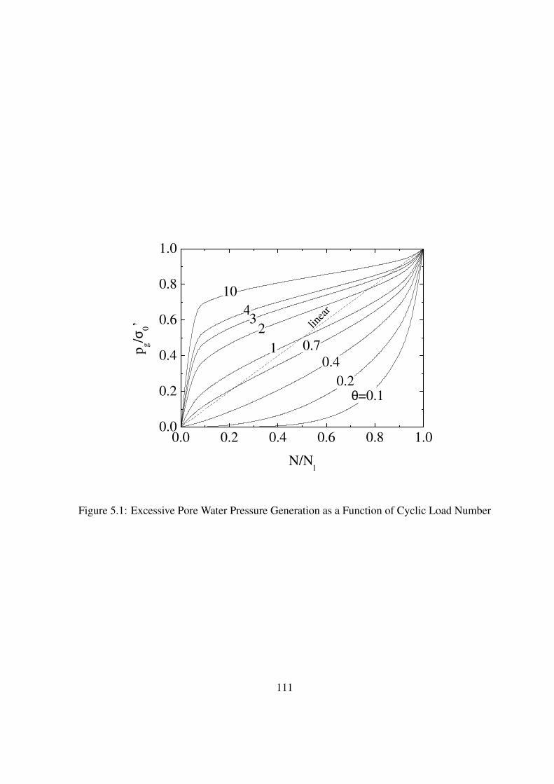
0.0 0.2 0.4 0.6 0.8 1.00.0
0.2
0.4
0.6
0.8
1.0
10
43
2
1 0.7
0.2
pg/σ
0’
N/Nl
θ=0.1
0.4
linea
r
Figure 5.1: Excessive Pore Water Pressure Generation as a Function of Cyclic Load Number
111
Linear Pore Water Generation Mechanism
The nonlinear mechanism from the experiment can be simplified to get the linear approximation.
In Fig. 5.1, when θ = 0.7, it is very close to the linear relationship which is also plotted. Seed
et al. (1975) proposed the linear mechanism as
pg
σ′0
=N
Nl
(5.19)
Thus, the source term for the pore water pressure generation should be
f =∂pg
∂t
=∂
∂t
(σ′0
t
TNl
)
=σ′0
TNl
For both mechanisms, the number of cyclic loadings to liquefaction Nl is a function of the
cyclic shear stress ratio (Seed and Booker 1978)
Nl =
(τ
ασ′0
)− 1β
(5.20)
where τ is the amplitude of the shear stress due to the cyclic loading and the two dimensionless
parameters α and β are functions of the soil type and the relative density.
5.3 Numerical Simulation of One-Dimensional Excessive Pore
Pressure Buildup Process
Even the simplified solutions to the analytical model introduced in this chapter are complicated,
and some assumptions such as isotropic can not be satisfied in real world. Analytical approach is
not always easy to be used. In this section, a numerical model is developed for the general one-
112

dimensional seabed response under waves. The results are used to compare with those from the
analytical solutions.
The residual pore water pressure equation is solved by using the open source CFD package
OpenFOAM OpenCFD (2006). This package is designed to solve partial differential equations
(PDEs) as long as the PDEs can be written in the specified format. Differential operators, such as
time derivative, Laplacican operator, and divergence, are implemented in the code. OpenFOAM
uses finite volume method to solve the equations. The residual pore water pressure equation is a
simple diffusion equation with a source term. It can be easily solved in OpenFOAM as follows.
fvMatrix PEqn
(
fvm::ddt(P)
- fvm::laplacian(C_nu,P)
==
src
);
PEqn.solve();
The term src is the source term. The shear stresses used to define the source term can be
calculated by using the numerical model introduced in chapter 4. This is the approach used by
Cheng et al. (2001). The shear stress can also be calculated by using the analytical solution of
oscillatory response of sea bed due to water waves (Jeng and Hsu 1996). Both approaches will
give the same results. For simplicity, the shear stresses and therefore the source term are defined
by the analytical solution. The schemes to discretize each term is defined in the file fvScheme
which is listed below.
113

ddtSchemes
default Euler;
gradSchemes
default Gauss linear;
grad(V) Gauss linear;
divSchemes
default none;
div(V) Gauss linear;
laplacianSchemes
default none;
laplacian(V) Gauss linear corrected;
interpolationSchemes
default linear;
114
snGradSchemes
default corrected;
Here, the time derivative is discretized by using the Euler method, and the Laplacian opera-
tor is discretized by using the Gauss theorem and a second order linear correction for the non-
orthogonality of the mesh. The details of each entry can be found in the manual of OpenFOAM.
5.4 Analytical Solution of One-Dimensional Excessive Pore
Pressure Buildup Model
Jeng et al. (2007) gives the analytical solutions to the excessive pore pressure generation model.
Under the conditions of finite depth, shallow and deep soil, the solutions can be expressed in
different forms. The details of the derivation can be found in Jeng et al. (2007). In this section,
only the results are listed. For the deep soil condition, the result given by Jeng et al. (2007) is not
easy to use. Based on this, a simplified estimation is proposed in this section using the asymptotic
method. Some errors in their paper are pointed out. Calculations are carried out to estimate the
time scale and maximum pressure depth.
The analytical solutions depend on the relative depth of the sediment, d/L, which is the ratio
between the sediment depth and the water wave length. Different authors have various criteria for
the relative depth (McDougal et al. 1989; Jeng et al. 2007). Table 5.1 lists the three regimes by
different authors. There are no clear-cut between different regimes, and both criteria are applicable.
115

Table 5.1: Criteria for the Relative DepthMcDougal et al. (1989) Jeng et al. (2007)
shallow d/L < 1/20 d/L < 1/10
finite 1/20 < d/L < 1/2 1/10 < d/L < 3/10
deep d/L > 1/2 d/L > 3/10
For finite and shallow soil depth, it is easy to solve the boundary value problem by using
Fourier series expansion method. For deep soil depth, Laplace transformation can be used for the
problem in the semi-infinite space.
5.4.1 Finite Depth Soil Solution
For the finite depth soil model, the residual pore water pressure can be expressed as
p =∞∑
n=1
an
(1− e−cvk2
nt/h2)
sin
(knz
h
)(5.21)
an =2h
cvk2n
∫ h
0
f(r) sin
(knr
h
)dr (5.22)
where f is the general source term as in the last section, and kn = (2n−1)π2
.
5.4.2 Shallow Soil Solution
For shallow soil, where the relative soil depth h/L < 0.1, the wave-induced shear stress can be
approximated as
τ = mPbz (5.23)
where the definition of m can be found in Jeng et al. (2007). Then the source term f can be
approximated as
f = az (5.24)
116

where
a =(1 + 2K0) γ
′
3T
[2mPb
α (1 + 2K0) γ′
] 1β
(5.25)
Then the excessive pore water pressure can be written using a Fourier series as
p =a
2cv
[(h2z − z3
3
)−
∞∑n=1
ane−cvk2
nt/h2
sin
(knz
h
)](5.26)
an =2
h
∫ h
0
(h2r − r3
3
)sin
(knr
h
)dr (5.27)
Jeng et al. (2007) did not give the final form of the Fourier series coefficients an. It is straight
forward to give a closed form
an =4h3
3k4n
[3 sin kn − kn
(3 + k2
n
)cos kn
](5.28)
5.4.3 Deep Soil Solution
For deep soil, where the relative soil depth h/L > 0.3, the source term can be approximated as
f = bze−λz (5.29)
where
λ =k
β(5.30)
and In Jeng et al. (2007), b is defined as
b = α
(k
m
) 1β
(5.31)
where m is defined the same as in the shallow soil solution. This is not correct since the wave
induced shear stresses are different for shallow soil and deep soil conditions. For shallow soil, the
shear stress can be approximated as a linear function of z with m as a linear coefficient. But for
117

deep soil, m can not be defined for the whole soil depth. This could be a typographical error. The
correct form of b should has the form as in Jeng and Seymour (2007)
b =γ′
T
1 + 2K0
3
[kPb
αγ′ 1+2K0
3
]1/β
(5.32)
Then the governing equation for the excessive pore water pressure can be written as
∂p
∂t= cv
∂2p
∂z2+ Aze−λz (5.33)
with boundary conditions
p(0, t) = p(z, 0) = 0 and∂p
∂z|z=∞,t = 0
In Jeng et al. (2007), the boundary condition at z = ∞ is set as p(∞, t) = 0. It is incorrect,
which will be shown later. Following the procedure in Jeng et al. (2007), Equation 5.33 is rescaled
according to
ξ = cvλ2t, P =
cvλ3p
Aand y = λz
The rescaled equation and initial/boundary conditions are
∂P
∂ξ=
∂2P
∂y2+ ye−y (5.34)
P (0, ξ) = P (y, 0) = 0 and∂P (∞, ξ)
∂y= 0
At steady state, the equation becomes
∂2P
∂ξ2+ ye−y = 0 (5.35)
118

Integrate the equation twice
P (y) = −e−y(2 + y) + C1y + C2
The coefficients C1 and C2 are determined by the boundary conditions
P (y = 0) = 0 : −e−0(2 + 0) + C1 ∗ 0 + C2 = 0 ⇒ C2 = 2
∂P (y = ∞)
∂y= 0 : e−0(2 + 0)− e−0 + C1 = 0 ⇒ C1 = 0
If the boundary condition at y = ∞ is set as in Jeng et al. (2007), then
P (y = ∞) = 0 : −e−∞(2 +∞) + C1 ∗∞+ 2 = 0
Then C1 can not be determined which means the boundary condition is not suitable.
Thus, the steady state solution is
P (y, ξ) = 2[1−
(y
2+ 1
)e−y
](5.36)
The full solution to equation 5.34 can be derived using Laplace transformation method. Jeng
et al. (2007) did not give the details of the derivation. The details of the laplace transformation and
inverse transformation are given in Appendix B. The full solution is
P (y, ξ) = 2
[1−
(y
2+ 1
)e−y − 1
π
∫ ∞
0
e−rξ
r(r + 1)2sin√
rydr
](5.37)
The analytical solution in Jeng et al. (2007) involves improper integration over infinite domain.
It is not easy to evaluate the solution. This difficulty is illustrated as follows.
The numerical evaluation of the improper integral in Eq. 5.37 needs some effort since the upper
limit of the integration is +∞ and the integrand is unbounded at r = 0. Fig. 5.2 shows the plots
119
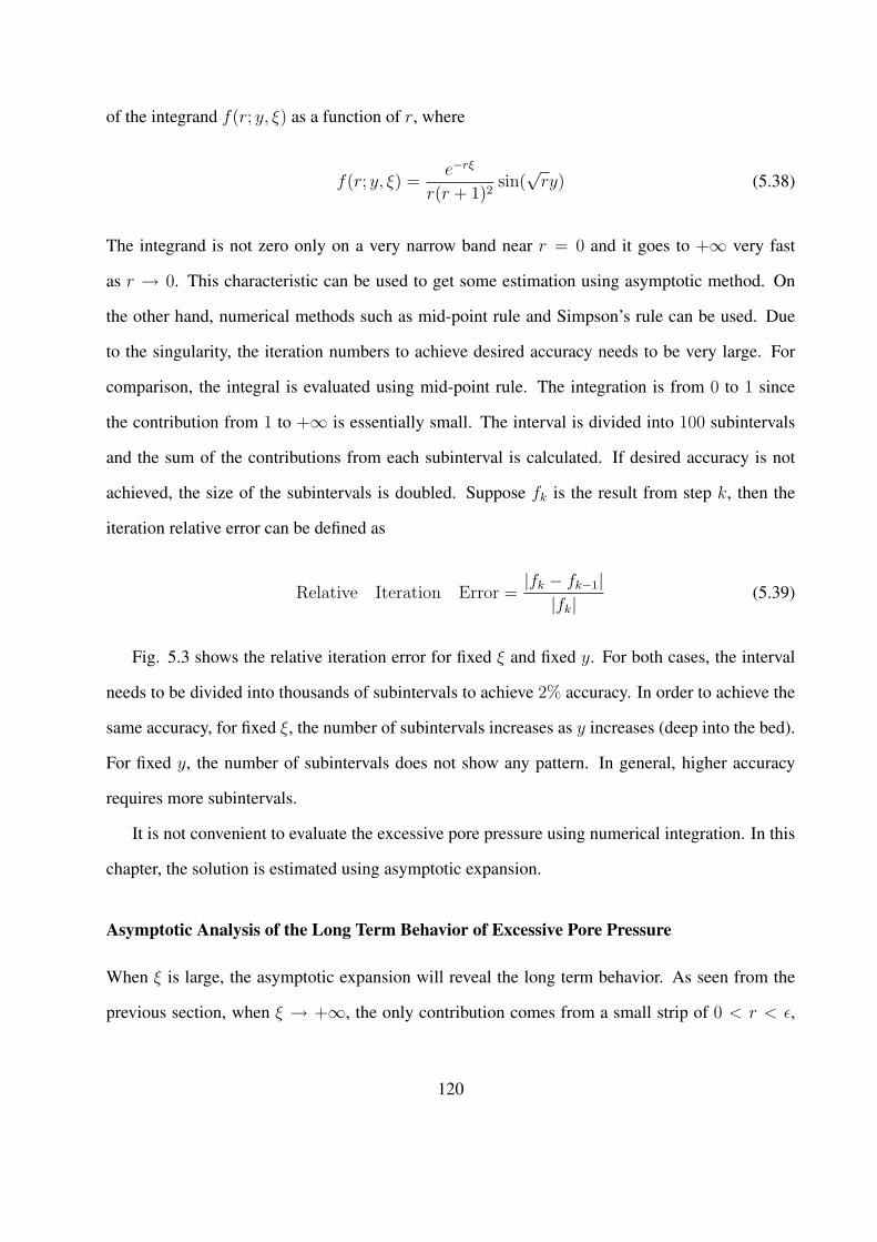
of the integrand f(r; y, ξ) as a function of r, where
f(r; y, ξ) =e−rξ
r(r + 1)2sin(
√ry) (5.38)
The integrand is not zero only on a very narrow band near r = 0 and it goes to +∞ very fast
as r → 0. This characteristic can be used to get some estimation using asymptotic method. On
the other hand, numerical methods such as mid-point rule and Simpson’s rule can be used. Due
to the singularity, the iteration numbers to achieve desired accuracy needs to be very large. For
comparison, the integral is evaluated using mid-point rule. The integration is from 0 to 1 since
the contribution from 1 to +∞ is essentially small. The interval is divided into 100 subintervals
and the sum of the contributions from each subinterval is calculated. If desired accuracy is not
achieved, the size of the subintervals is doubled. Suppose fk is the result from step k, then the
iteration relative error can be defined as
Relative Iteration Error =|fk − fk−1|
|fk| (5.39)
Fig. 5.3 shows the relative iteration error for fixed ξ and fixed y. For both cases, the interval
needs to be divided into thousands of subintervals to achieve 2% accuracy. In order to achieve the
same accuracy, for fixed ξ, the number of subintervals increases as y increases (deep into the bed).
For fixed y, the number of subintervals does not show any pattern. In general, higher accuracy
requires more subintervals.
It is not convenient to evaluate the excessive pore pressure using numerical integration. In this
chapter, the solution is estimated using asymptotic expansion.
Asymptotic Analysis of the Long Term Behavior of Excessive Pore Pressure
When ξ is large, the asymptotic expansion will reveal the long term behavior. As seen from the
previous section, when ξ → +∞, the only contribution comes from a small strip of 0 < r < ε,
120

0.00 0.02 0.04 0.06 0.08 0.10-50
0
50
100
150
200
250
300
350
f(r)
r
y=1
y=5
y=10
(a)
0.00 0.02 0.04 0.06 0.08 0.10 0.12-20
0
20
40
60
80
100
120
140
160
f(r)
r
ξ=100
ξ=300
ξ=1000
(b)
Figure 5.2: Plot of the Integrand: (a) Same ξ (ξ = 100) (b) Same y (y = 5)
121
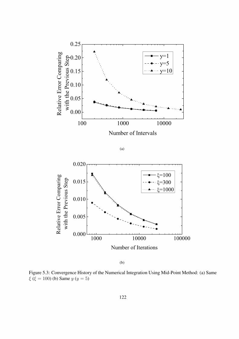
100 1000 10000
0.00
0.05
0.10
0.15
0.20
0.25
Rel
ativ
e Er
ror C
ompa
ring
with
the
Prev
ious
Ste
p
Number of Intervals
y=1 y=5 y=10
(a)
1000 10000 1000000.000
0.005
0.010
0.015
0.020
Rel
ativ
e Er
ror C
ompa
ring
with
the
Prev
ious
Ste
p
Number of Iterations
=100 =300 =1000
(b)
Figure 5.3: Convergence History of the Numerical Integration Using Mid-Point Method: (a) Sameξ (ξ = 100) (b) Same y (y = 5)
122

where ε ∼ o(1). Then1
(r + 1)2∼ (1− r)2 ∼ 1− 2r (5.40)
Plug into the integral,
∫ ∞
0
e−rξ
r(r + 1)2sin(
√ry)dr ∼
∫ ∞
0
e−rξ 1− 2r
rsin(
√ry)dr
=
∫ ∞
0
e−rξ
rsin(
√ry)dr − 2
∫ ∞
0
e−rξ sin(√
ry)dr
∼ πerf(y
2√
ξ)−
√πy
ξ3/2e−
y2
4ξ
So
P (y, ξ) ∼ 2
[1−
(y
2+ 1
)e−y − erf(
y
2√
ξ) +
y√πξ3/2
e−y2
4ξ
]as ξ → +∞ (5.41)
The error function can be approximated as
erf(x) =
[1− exp
(−x2 4/π + ax2
1 + ax2
)] 12
for x ≥ 0 (5.42)
where
a = − 8
3π
π − 3
π − 4(5.43)
In Fig. 5.4, the integral as a function of ξ and y is plotted. Both the results from numerical
method and asymptotic method are shown. The results from both methods are almost identical.
For the same y, the integral decreases to zero as time ξ increases to infinity. At the same time ξ,
the integral increases to an asymptotic value as y goes deep into the soil.
Fig. 5.5 shows the relative error using the asymptotic estimation. The exact value of the
integral is calculated using the numerical method with the successive change of the iterations less
than 0.1%. The maximum relative error is around 1.5%. When y increases, i.e., deep into the soil,
the relative error increases. When time ξ increases, the relative error also increases.
123

0 100 200 300 400 5000.40.60.81.01.21.41.61.82.02.2
Inte
gral
y=5 Numerical y=5 Asymptotic y=10 Numerical y=10 Asymptotic
(a)
0 10 20 30 40 50 600.0
0.5
1.0
1.5
2.0
2.5
3.0
3.5
Inte
gral
y
=100 Numerical =100 Asymptotic =500 Numerical =500 Asymptotic
(b)
Figure 5.4: Integral Evaluation Using Numerical Method and Asymptotic Estimation: (a) Same ξ(ξ = 100) (b) Same y (y = 5)
124

0 100 200 300 400 5000.0
0.5
1.0
1.5
2.0
y=5 y=10
Rel
ativ
e Er
ror (
%)
(a)
0 10 20 30 40 500.0
0.5
1.0
1.5
2.0
=100 =500R
elat
ive
Erro
r (%
)
y
(b)
Figure 5.5: Relative Error Using the Asymptotic Approximation: (a) Same ξ (ξ = 100) (b) Samey (y = 5)
125

Due to the diffusion nature of the equation, it will take infinite time to reach the steady state.
It is useful to get some information on where the pore pressure will reach 99% of the maximum
value and for each depth, how long it will take to reach 99% of its steady state. Using the numerical
method and asymptotic analysis, the excessive pore pressure is plotted in Fig. 5.6.
0.0 0.2 0.4 0.6 0.8 1.0 1.2 1.4 1.6 1.8 2.050
40
30
20
10
0
steady state
=1000=500
Dep
th y
Excessive Pore Pressure P(y, )
Numerical Asymptotic
=100
Figure 5.6: Excessive Pore Pressure Development for Deep Soil
At steady state, the position y = y99% where the pore pressure reaches 99% of the maximum
value can be solved using
2[1−
(y
2+ 1
)e−y
]= 2 ∗ 0.99 ⇒ y99% = 5.99
At y = y99%, the time it takes for the excessive pore pressure to reach 99% of local maximum
value (i.e. Pmax = 1.98) is about ξ = 116533. Fig. 5.7 shows the relationship between the time and
the percentage of the local maximum pore pressure at y = y99%. With the percentage increasing,
the time needed increases.
126
90 92 94 96 98 10010
3
104
105
ξ
Percentage of Pmax
at y=y99%
Figure 5.7: Excessive Pore Pressure Development at y = y99%
127

5.5 Comparison Between Numerical and Analytical Solutions
In this section, the results from both numerical and analytical solutions are compared for different
soil and wave conditions. Three different depths of soil are calculated using the model developed
in the previous sections. For shallow and finite depth soil models, comparisons are done between
the numerical and analytical solutions. For deep soil model, asymptotic solution is also compared.
Numerical simulations are carried out using a uniform grid along the depth. The total grid number
for all simulations is 1000. The numerical accuracy can be improved when the total number of grid
is increased, especially in the region where the residual pressure gradient is high. For the purpose
of this chapter, 1000 grids along the depth give a good representation of the solution.
The test cases used in this chapter are from Clukey et al. (1985) where pressure accumulation
experiments are done in a small wave tank. Wave-induced liquefaction data in this chapter is also
used by many authors (McDougal et al. 1989; Cheng et al. 2001; Jeng et al. 2007). Pa‘rameters
for the soil used in the experiments are listed in Table 5.2. Only Run 3-1 of Clukey et al. (1985) is
used in this chapter and the liquefaction results from the experiment is listed in Table 5.3. For the
soil depth used in Clukey et al. (1985), d = 0.84m, and the wave length in Run 3-1, L = 3.473m,
the relative soil depth is d/L = 0.242. This falls in the range of finite to deep soil. In order to
verify the models in this chapter, soil depth d is set to be 0.11m, 0.84m and 10m for shallow, finite,
and deep soil models. Only when d = 0.84m, the model can be validated with experiments.
Table 5.2: Soil Parameters from Clukey et al. (1985)Poisson’s ration 0.49
Shear modulus (N/m2) 5.6× 10⁵
Submerged weight (N/m2 8.5× 10³
Permeability (m/s) 4× 10⁻⁸
Porosity 0.46
Lateral earth pressure coefficient 0.4
α 0.246
β 0.165
cν 0.000156
128

Table 5.3: Liquefaction Experiment Results of Clukey et al. (1985) (Run 3-1)Wave Period Wave Height Water Depth Soil Depth Residual Pore Pressure
(s) (m) (m) (m) Depth (m) Pressure(kN/m2)
1.76 0.22 0.5 0.84 0.04 0.77
0.10 0.96
0.35 2.20
0.47 2.54
5.5.1 Comparison for Shallow Soils
For the shallow soil model, since there is no measurement, the only comparison is between the re-
sults of numerical model and analytical model. Here, the soil depth is set as 0.11m, corresponding
to d/L = 0.032. The results are plotted in Fig. 5.8. Both results agree with each other. The pore
pressure at the soil surface is zero due to the boundary condition. The maximum pore pressure is
always at the impermeable boundary at z = d. The steady state solution is also plotted. From the
figure, the result at t = 100s is close to steady state.
0 1x10⁻⁷
2x10⁻⁷
3x10⁻⁷
4x10⁻⁷
1.0
0.8
0.6
0.4
0.2
0.0
steady state
t=100 st=10 s
z/d
Residual Pore Pressure (N/m2)
Numerical
Analytical
t=1 s
Figure 5.8: Comparison between Numerical and Analytical Solutions for Shallow Soil (d/L =0.032)
129

5.5.2 Comparison for Finite Depth Soils
Fig. 5.9 shows the comparison between the results of the numerical model and the analytical
model. Here the soil depth is set as the same as in the experiment of Clukey et al. (1985). Again,
both results agree with each other very well. Steady state solution is also plotted. The solution at
t = 10000s is close to steady state. The shape of the residual pore pressure for finite depth soil is
similar to that of shallow soil where residual pressure is zero at the surface and maximum pressure
is achieved at the bottom. But for finite depth soil, the time to get steady state is longer than that
of shallow depth.
0.0 4.0x10²
8.0x10²
1.2x10³
1.6x10³
2.0x10³
2.4x10³
1.0
0.8
0.6
0.4
0.2
0.0
t=10 s
t=100 st=1000 s
Numerical
Analytical
z/d
Residual Pore Pressure (N/m2)
steady state
t=10000 s
Figure 5.9: Comparison between Numerical and Analytical Solutions for Finite Depth Soil (d/L =0.242)
For finite deposit soil, the experiment results can be used to validate the model. In Fig. 5.10,
the data from Clukey et al. (1985) is plotted. The model used in this chapter gives fairly good
results
130

0.0 5.0x10²
1.0x10³
1.5x10³
2.0x10³
2.5x10³
3.0x10³
1.0
0.8
0.6
0.4
0.2
0.0
Close to Failure
z/d
Residual Pore Pressure (N/m2)
Numerical
Experimental
Failure
Figure 5.10: Comparison between Numerical and Experimental Results for Finite Depth Soil(d/L = 0.242)
5.5.3 Comparison for Deep Soils
For the deep soil case, the soil depth is set as d = 10m, which corresponds to d/L = 2.879. The
comparison between the numerical solution and the analytical solution is plotted in Fig. 5.11. At
steady state, the whole soil column has almost the same residual pressure except that at the top
portion the pressure decreases to zero due the effect of diffusion. The time for the deep soil case
to get to close to the steady state is far more than the previous two cases (shallow and finite depth).
From the figure, at t = 100000s, the maximum pore pressure almost reached its final state. The
majority part of the soil column below that point is still far away from steady state.
The comparison is also done between the numerical results and the asymptotic solutions. It
is plotted in Fig. 5.12. The agreement is clearly shown in the figure. The asymptotic solution
proposed in this chapter can be used to get a faster solution of the problem.
131
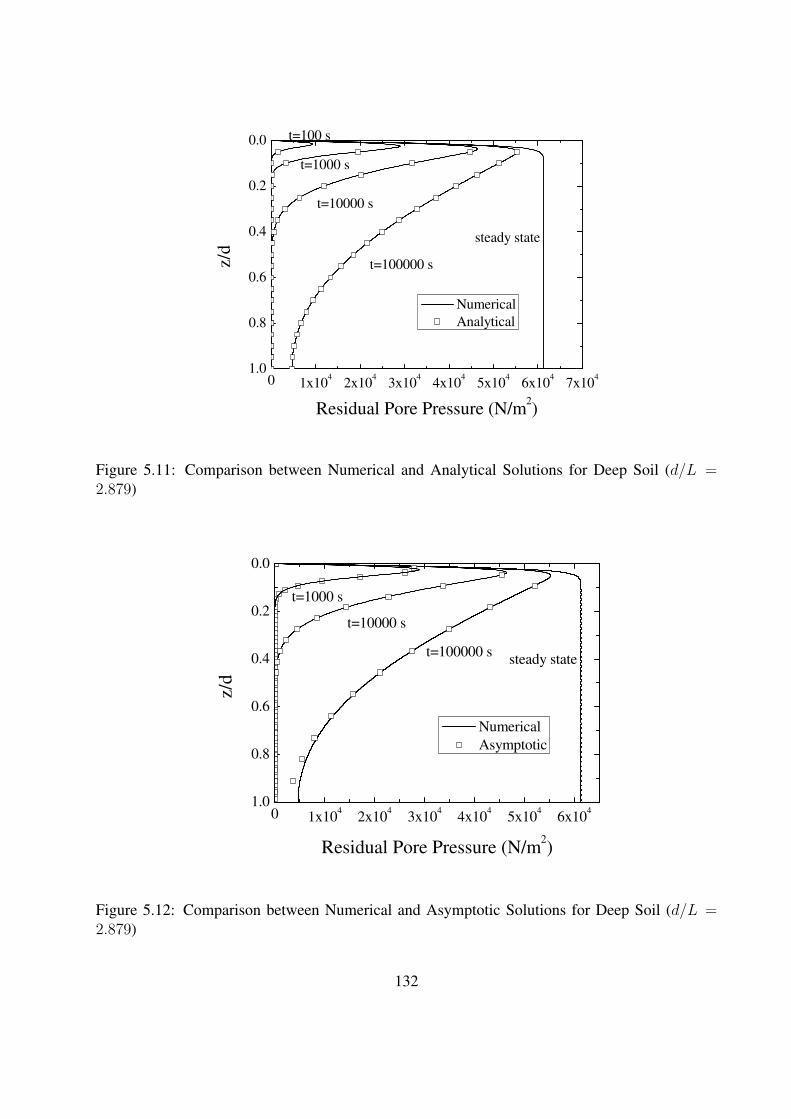
0 1x10⁴
2x10⁴
3x10⁴
4x10⁴
5x10⁴
6x10⁴
7x10⁴
1.0
0.8
0.6
0.4
0.2
0.0
Numerical
Analytical
t=100000 s
t=10000 s
t=1000 s
z/d
Residual Pore Pressure (N/m2)
t=100 s
steady state
Figure 5.11: Comparison between Numerical and Analytical Solutions for Deep Soil (d/L =2.879)
0 1x10⁴
2x10⁴
3x10⁴
4x10⁴
5x10⁴
6x10⁴
1.0
0.8
0.6
0.4
0.2
0.0
t=1000 s
t=10000 s
z/d
Residual Pore Pressure (N/m2)
Numerical
Asymptotic
steady statet=100000 s
Figure 5.12: Comparison between Numerical and Asymptotic Solutions for Deep Soil (d/L =2.879)
132
5.6 Numerical Model For Phase-Resolved Residual Pore
Pressure and Liquefaction Potential Under Waves
The one-dimensional model introduced in the previous sections is only for the period-averaged
residual pore pressure. It is applicable when the interaction is only between the wave and the
seabed. In reality, the situation will be more complicated and the application of the one-dimensional
model is limited. In engineering practice, it is important to know the liquefaction potential around
the structure foundation or pipe lines. Because of the presence of these structures, the water wave
field in the vicinity will be changed. Therefore, the wave-induced shear stress in the soil will also
be changed. With one-dimensional model, it is impossible to capture the interactions between
waves, structure, and sea bed. The three-dimensional numerical model developed in Chapter 4
has been used to investigate the oscillatory response of the sea bed under waves. In this section, a
tentative effort is made to modify the model to study the residual response of the seabed.
The governing equation for the force balance of the soil is the same as Eq. 5.1. For the storage
equation, an extra source term corresponding to the excessive pore pressure generation is added.
The new storage equation has the form
n
K ′∂p
∂t+
∂
∂t(∇ · v) =
k
γ∇2p +
n
K ′ f (5.44)
where f is given as in the previous section for the one-dimensional period averaged model.
5.6.1 Two-Dimensional Test Case for the Experiment by Clukey et al.
(1985)
Fig. 5.13 shows the domain of the problem. The depth of the soil is 0.84 m and the length of the
domain is set as the water wave length. Left and right boundaries are periodic. The pressure at the
bed surface is set as the progressive water wave pressure. At the bottom, slip boundary condition
is set for the displacement and zero gradient is set for the pressure (i.e., impermeable).
133

Per
iodic
Per
iod
ic
x
yWave Pressure On the Bed
p=pbcos(kx- t)
d =
0.8
4m
L = 3.473 m
Figure 5.13: Schematic View for the 2D Residual Liquefaction Test Case
Total simulation time for this case is 20T , where T is the wave period. In Fig. 5.14 and
Fig. 5.15, both the water wave pressure field and the pore pressure field are plotted for different
moments during one wave period. At the beginning of simulation, not too much residual pressure
has been generated. The pressure field is similar to that of momentary liquefaction, i.e., the source
term effect is negligible. With time increases, the pore water pressure generated is much more than
which is dissipated. Except for the near surface region, the whole soil column almost has uniform
residual pore pressure (see Fig. 5.15).
Two probe points are placed in the center plane (x = 1.737m) of the simulation domain to
record the time development of residual pore pressure. Those two probe points are at z = −0.1m
and z = −0.8m. The recorded residual pore pressure is plotted in Fig. 5.16. Also plotted is the
period-average of both signals. At both probe points, the pressure signal oscillates around the trend
line (the period-average). It is clear that the residual pore pressure increases to some asymptotic
value for both depth. The asymptotic value for z = −0.1m is lower than that for z = −0.8m
which is as expected by analytical solution.
In Fig. 5.17, the residual pore pressure profiles at the center plane x = 1.737m in one typical
wave period are plotted. The data plotted is from the last simulated wave period (t = 19T → 20T ).
134
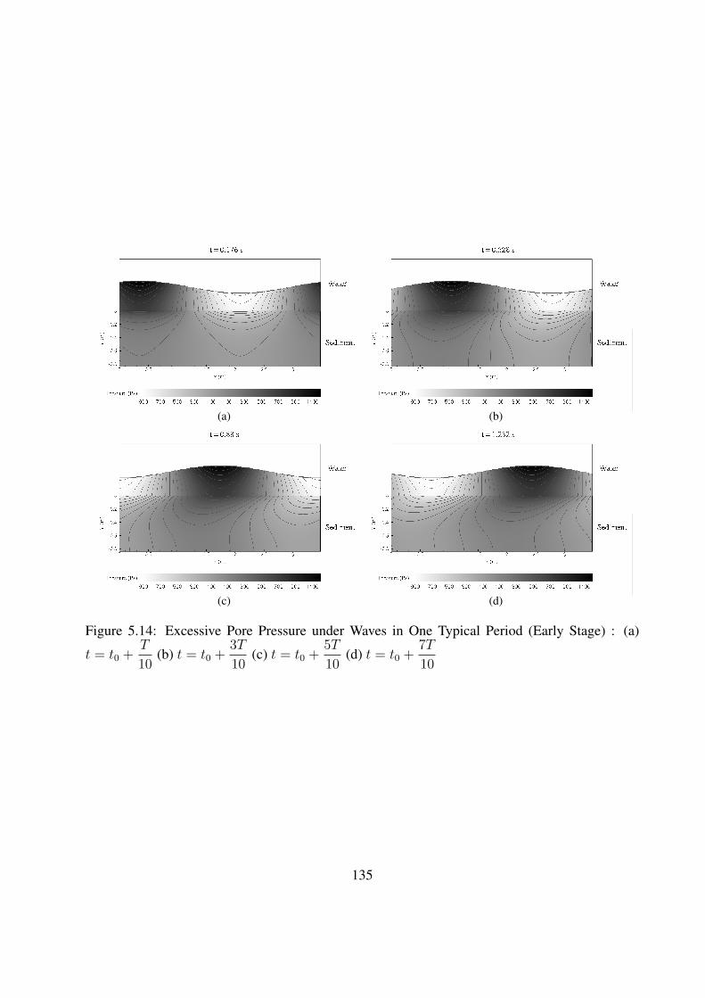
(a) (b)
(c) (d)
Figure 5.14: Excessive Pore Pressure under Waves in One Typical Period (Early Stage) : (a)
t = t0 +T
10(b) t = t0 +
3T
10(c) t = t0 +
5T
10(d) t = t0 +
7T
10
135

(a) (b)
(c) (d)
Figure 5.15: Excessive Pore Pressure under Waves in One Typical Period (Later Stage)): (a) t =
t0 +T
10(b) t = t0 +
3T
10(c) t = t0 +
5T
10(d) t = t0 +
7T
10
136

0 5 10 15 20 25 30 35 40 45
0
500
1000
1500
2000
2500
3000
z = -0.8 m
Resi
du
al
Po
re P
ress
ure
(P
a)
Time (s)
Pressure Time Serie
Period-Averaged
z = -0.1 m
Figure 5.16: Time Series For the Residual Pore Pressure at Different Depth
From the figure, the residual pore pressure during this last simulated wave period still oscillates
but is close to steady state solution. At the upper portion near the bed surface, the amplitude of the
pore pressure oscillation (p1) is larger than that at the lower portion of the soil (p2).
The period-averaged residual pore pressure profile is plotted in Fig. 5.18. For comparison,
the one-dimensional analytical solution is also plotted. A large amount of difference between
the one-dimensional and two-dimensional results is observed. However, the result from the two-
dimensional model is closer to the experiment data. One reason could be that the one-dimensional
model neglects the variation along the x direction. The neglect of x direction variation will change
the shear stress which is a function of ∂u/∂x and therefore introduce error for residual pore pres-
sure.
5.7 Discussion
The one-dimensional residual pore pressure buildup model used in this chapter is only for the
period-averaged pressure. It is only valid in the sense of averaging. This model is good for the
137

-1000 0 1000 2000 3000
-0.8
-0.6
-0.4
-0.2
0.0
dep
th z
(m
)
Residual Pore Pressure (Pa)
t = t0+T/10
t = t0+3T/10
t = t0+5T/10
t = t0+7T/10
p1
p2
Figure 5.17: Residual Pore Pressure Profiles at the Center Plane in One Typical Wave Period
0 500 1000 1500 2000 2500 30001.0
0.8
0.6
0.4
0.2
0.0
z/d
Residual Pressure (Pa)
1D Model
2D Model
Experiment
Failure
Close to Failure
Figure 5.18: Schematic View for the 2D Residual Liquefaction Test Case
138

investigation of the liquefaction trend in the soil. The detailed pore pressure buildup process
(oscillation around the mean value) is lost.
The classification of three different regimes of soil (shallow, finite depth, and deep) are not so
apparent. For shallow soil, the shear stress induced by the waves should be approximately linear
with the depth. For deep soil, the shear stress should be able to be written in the general form
ye−y. If the approximated shear stress is far away from these forms, the proposed solutions can
not be used. As pointed out by Cheng et al. (2001), the solutions are sensitive to the shear stress
(the sensitivity depends on the soil regime and the parameter β), and different approximation of
the shear stress will lead to huge difference in the solutions. In general, the finite depth model
(with the full solution of the shear stress) is valid for all three regimes. No approximation is made
for the shear stress, therefore, it can be used as a general solution.
The model used in this chapter depends on the coefficients from the experiment (especially
α and β). These coefficients are only for the soil used in the experiment. When soil conditions
change, these coefficients should also change. As mentioned earlier, the results are very sensitive
to these coefficients. More experimental work should be done to give good description of these
coefficients.
5.8 Conclusion
In this chapter, a one-dimensional period-averaged residual pore pressure model is introduced. The
governing equation for the residual pore water pressure is a diffusion equation with a source term
which represents the generation of the pore pressure. Although this source term comes from the
analytical derivation of the equation, it is given by experiments. Linear and nonlinear forms of
the source term were proposed by De Alba et al. (1976). For nonlinear form of the source term,
the governing equation can only be solved numerically while for linear form of the source term, it
can be solve both numerically and analytically. According to the relative depth d/L, the soil can
be classified into three different regimes (shallow, finite depth, and deep soils). In each regime,
139

the analytical solution for wave induced shear stress is used for the source term. Based on the
solutions given by Jeng et al. (2007), some errors are corrected in this chapter and revised forms
of the solutions are given.
For deep soil model, the solution by Jeng et al. (2007) has an improper integral and is not easy
to use. The difficulty to evaluate the solution numerically due to the singularities is illustrated in
this chapter with the help of examples. Based on the form of the improper integral, an asymptotic
solution is proposed in this chapter. This asymptotic solution has a closed form and is easy to
evaluate.
Besides an analytical approach, numerical solutions for the residual pore water pressure are
also given by using the differential equation solver package OpenFOAM. The results from analyt-
ical solutions, numerical solutions, and asymptotic estimations are compared. Perfect agreement
has been achieved. For finite depth soil, the experiment data of Clukey et al. (1985) are used for
validation. The models in this chapter predict the liquefaction fairly well.
A numerical model is also introduced for the phase-resolved residual pore pressure. The basic
idea of adding a source term to the governing equation is used. The source term has the same form
as that of the period-averaged residual pore pressure model. Test cases show that this model gives
good results when comparing with the one-dimensional period-averaged model.
140

Chapter 6
Summary
This thesis addresses two mechanisms in the interaction between water, sediment, and structures,
namely scour and liquefaction. Both mechanisms are closely related to each other. Numerical
models are developed to simulate and study the process.
6.1 Numerical Models for Scour
For scour, two-dimensional and three-dimensional models are developed. Two-dimensional model
is suitable for large scale and long term scour process, while the three-dimensional model is suit-
able for detailed local scour around structures.
6.1.1 Two-Dimensional Scour Model
The coupled model of two-dimensional SWEs and sediment transport on unstructured mesh was
implemented for scour problems on complex domains. This coupled modeling approach is neces-
sary when the scour process is rapid. When the scour process is slow (such as long term aggrada-
tion/degradation of natural rivers), both the usual quasi-steady approach and the coupled approach
can give good results. However, the numerical stability of the quasi-steady approach will present
difficulty. High order discretization of the Exner equation may lead to non-physical oscillations
which could be incorrectly interpreted as ripples and sand waves. Low order discretization of the
Exner equation may under-estimate the amplitude of the real sand wave or even smear it out. The
hyperbolic nature of the Exner equation (even though there is dispersion effect in the equation)
makes it possible to couple it with SWEs and to use Godunov schemes. The coupled model with
141

a higher order Godunov scheme proposed in this thesis can capture the real wave accurately while
controlling the growth of non-physical oscillations.
An asymptotic analysis was done to gain an insight about the wave speed structure and to
construct an explicit expression for the Roe’s flux. It also gave a fast and accurate evaluation of
the eigenvalues/vectors. Comparing to the numerical iteration method for the eigen-system, the
asymptotic approximation is far more efficient. For the test case used in this paper, the average
computational time can be reduced by approximately 64%.
The interpolation method of the TVD scheme used in the current numerical model for the
upwind ratio of consecutive gradients is based on the virtual upwind node. The basic assumption
is that the gradient from upwind node to downwind node is the same as that from center node
to downwind node. This assumption simplifies the calculation and reduces the stencil. Future
research is needed on the comparison of different interpolation methods and TVD schemes.
6.1.2 Three-Dimensional Scour Model
Numerical model FOAMSCOUR for local scour with free surface and automatic mesh deformation
is proposed. The turbulence model used is the simple two equation k − ε model. Other turbulence
models, even large eddy simulation, can be used to improve the accuracy of the fluid flow field
simulation. All these models are readily implemented in OpenFOAM. The free surface is modeled
by VOF method while the scour process is modeled by moving mesh method. These two methods
for moving boundaries(free surface and bed) are coupled together. Each method has its merits
and shortcomings. Eulerian approach can be used to capture the complex scour profiles. Flow
field is coupled with sediment transport (both bed load and suspended load) using a quasi-steady
approach. Parallel computations are used to reduce the CPU time which is usually tremendously
large for morphological simulations.
Numerical simulations for turbulent wall jet scour and wave scour around large vertical cylin-
der are carried out and compared with experiments. Good results have been obtained using the
proposed modeling approach. Velocity field and other flow field characteristics compare fairly
142
well with experimental observations. The maximum scour depths and local scour profile fit well
with the experiment data. Further research is needed to investigate the effects of turbulence model
for free surface waves (especially for near breaking and breaking waves) and to study the possibil-
ity of using an Eulerian approach for morphological modeling.
For the effect of the free water surface, the following conclusions are drawn. For the submerged
wall jet case, the water depth in the flow domain is much bigger than the jet opening and the free
surface changes very slowly. This makes the rigid-lid approximation a reasonable one. For scour
around slender piles under waves, the rigid-lid assumption is also valid since the most important
mechanism here is the vortex shedding and horseshoe vortex. However, for the wave-induced
scour around large piles, it is unreasonable to use the rigid-lid approximation since the dominant
mechanism here is the phase-resolved component of the wave flow and the steady streaming.
In the current numerical model, the two moving surfaces (water free surface and moving bed)
are captured by different approaches, namely Eulerian and Lagrangian approaches. The free sur-
face is solved by the CICSAM VOF scheme, which is an Eulerian approach. The moving bed is
captured by the mesh deformation method, which is a Lagrangian approach. The scour test cases
in the paper are relatively simple. For more complicated problems, if there are objects interacting
with the fluid phase and the bed, the moving mesh technique will not be appropriate. The interface
between the object, water and bed is very complicated and changing with time. Simply moving
the grid point along the interface will be not feasible. For such cases, the Eulerian approach (VOF
or LSM) can be used to implicitly track the interface. This could provide new research direction
in the scour problem and currently is being explored by the authors.
There is some limitation when using the mesh deformation approach to capture the interaction
of many phases. The mesh deformation approach is hard to implement with the presence of in-
teraction between moving objects and the bed or when the boundary movement is irregular. Also,
when the amplitude of the boundary movement is big enough, the mesh may be highly distorted,
and the deteriorated mesh quality will make the computation difficult to converge, eventually lead-
ing to unstable solutions. In order to avoid these problems, the dynamic mesh approach should be
143

used. In the dynamic mesh approach, mesh cells can be split or merged when necessary. How-
ever, when comparing them with mesh deformation, the dynamic mesh approach is more difficult.
Combining these two approaches can be promising for scour problems where the scour pattern is
complicated and the scour/deposition depth is very large.
6.2 Numerical Models for Liquefaction
Two different liquefaction mechanisms (momentary and residual liquefactions) are considered in
this thesis.
6.2.1 Momentary Liquefaction
The numerical model in this paper can solve the coupling problem between waves, object (struc-
ture) and sea bed response. The wave induced shear stress and pore pressure in the soil is governed
by the Biot consolidation equation. The free surface is modeled by the VOF method and the wa-
ter wave is generated by numerical wave maker boundary conditions. Instead of using the finite
element method to do stress analysis inside the bed material (which is the traditional method used
in geotechniques), an iterative numerical scheme is proposed to solve the Biot consolidation equa-
tion using finite volume method. The new scheme shows a fast convergence rate as well as a high
accuracy. The coupling between water waves and the sea bed is through pressure and stress con-
dition on common boundaries. Two numerical tests of the proposed scheme is carried out. First,
the numerical case tests the consolidation solver part of the numerical model. Good agreement
with analytical results is obtained. The second case is a 3D test to study the interaction between
the waves, the sea bed and the object. A box is half buried in the wave tank. More complicated
geometries can be simulated as well. From the results, excessive pore pressure of the sea bed as
well as the liquefaction potential can be analyzed.
For geotechnical problems, a realistic stress-strain constitutive relationship is one of the most
important aspects for the ability of the numerical model to reproduce real situations. In this thesis,
144
the simple linear isotropic elastic model is used to describe the soil skeleton. More advanced
and accurate constitutive models (such as variable elasticity, elasto-plastic model and visco-plastic
model, etc.) can be easily incorporated in the current numerical code. The anisotropic effect can
also easily come into the model since the code is based on the tensorial description of the equations
and anisotropic tensors can be included inside the differential operators.
In the three-dimensional test case, the object is assumed to be at fixed position during the
computation. This is not always true since when liquefaction occurs, the soil can no longer support
the object and the object will move. Even without liquefaction, the object could rotate or slide
under the influence of fluid force. All these make the problem extremely complicated and it is
impossible to include all factors into the numerical model. However, by fixing the object in one
position, it is possible to investigate the possibility of liquefaction and analyze the dynamics of the
system. This could be useful for engineers to design structures and foundations to prevent damage
under extreme conditions.
6.2.2 Residual Liquefaction
One-dimensional period-averaged residual pore pressure model is introduced. The governing
equation for the residual pore water pressure is a diffusion equation with a source term which
represents the generation of the pore pressure. Although this source term comes from the ana-
lytical derivation of the equation, it is given by experiments. Linear and nonlinear forms of the
source term were proposed in the literature. For a nonlinear form of the source term, the governing
equation can only be solved numerically while for a linear form of the source term, it can be solve
both numerically and analytically. According to the relative depth d/L, the soil can be classified
into three different regimes (shallow, finite depth, and deep soils). In each regime, the analytical
solution for the shear stress is used for the source term. Based on the solutions given by Jeng et al.
(2007), some errors are corrected in this thesis, and revised forms of the solutions are given.
For the deep soil model, the solution by Jeng et al. (2007) has an improper integral and is not
easy to use. The difficulty to evaluate the solution numerically due to the singularities is illustrated
145
in this thesis with examples. Based on the form of the improper integral, an asymptotic solution is
proposed. This asymptotic solution has a closed form and is easy to evaluate.
Besides an analytical approach, numerical solutions for the residual pore water pressure are
also given. The results from the analytical solutions, the numerical solutions, and the asymptotic
estimations are compared. Perfect agreement has been achieved between both. For the finite depth
soil, the experimental data of Clukey et al. (1985) are used for validation. The proposed model
predicts liquefaction fairly well.
146

Appendix A
Asymptotic Analysis of Eigenvalues
A.1 Eigen-systems When uξ 6= 0
The regular expansion is used to approximate the roots of Eqn. 2.27. Assume
λ = λ0 + ελ1 + O(ε2) (A.1)
Substituting Eqn. A.1 into Eqn. 2.27 and expanding give
[(1− 1
Fr2
)λ0 − 2λ2
0 + 3λ30
]+
[1− λ0 + kλ1 − 4λ0λ1 + 3λ2
0λ1
]ε + O(ε2) = 0 (A.2)
Equating the coefficients of like powers of ε gives
(1− 1
Fr2
)λ0 − 2λ2
0 + 3λ30 = 0 (A.3)
1− λ0 + kλ1 − 4λ0λ1 + 3λ20λ1 = 0 (A.4)
Solving these equations gives the eigenvalues as
λ(1) =ε
1Fr2 − 1
(A.5)
λ(2) = 1 +1
Fr+
ε
2(
1Fr
+ 1) (A.6)
λ(3) = 1− 1
Fr− ε
2(
1Fr− 1
) (A.7)
147
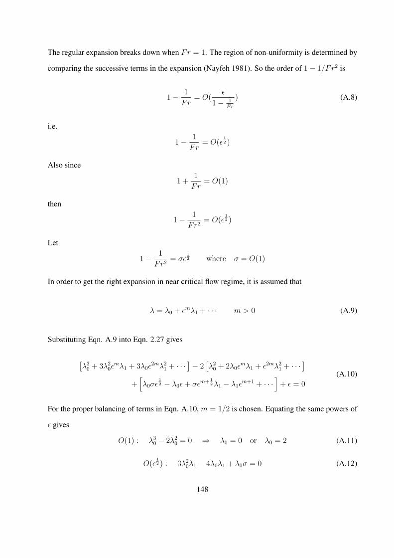
The regular expansion breaks down when Fr = 1. The region of non-uniformity is determined by
comparing the successive terms in the expansion (Nayfeh 1981). So the order of 1− 1/Fr2 is
1− 1
Fr= O(
ε
1− 1Fr
) (A.8)
i.e.
1− 1
Fr= O(ε
12 )
Also since
1 +1
Fr= O(1)
then
1− 1
Fr2= O(ε
12 )
Let
1− 1
Fr2= σε
12 where σ = O(1)
In order to get the right expansion in near critical flow regime, it is assumed that
λ = λ0 + εmλ1 + · · · m > 0 (A.9)
Substituting Eqn. A.9 into Eqn. 2.27 gives
[λ3
0 + 3λ20ε
mλ1 + 3λ0ε2mλ2
1 + · · · ]− 2[λ2
0 + 2λ0εmλ1 + ε2mλ2
1 + · · · ]
+[λ0σε
12 − λ0ε + σεm+ 1
2 λ1 − λ1εm+1 + · · ·
]+ ε = 0
(A.10)
For the proper balancing of terms in Eqn. A.10, m = 1/2 is chosen. Equating the same powers of
ε gives
O(1) : λ30 − 2λ2
0 = 0 ⇒ λ0 = 0 or λ0 = 2 (A.11)
O(ε12 ) : 3λ2
0λ1 − 4λ0λ1 + λ0σ = 0 (A.12)
148

For λ0 = 0, Eqn. A.12 is satisfied automatically and λ1 should be calculated through higher order
terms. For λ0 = 2, Eqn. A.12 gives
λ1 = − σ
3λ0 − 4= −σ
2
O(ε) : 3λ0λ21 − 2λ2
1 − λ0 + σλ1 + 1 = 0 (A.13)
For λ0 = 0, Eqn. A.13 gives
λ1 =σ ±√σ2 + 8
4
So in the region of 1− 1Fr2 = O(ε
12 ), the eigenvalues are
λ(1) = 2− σ
2ε
12 =
3
2+
1
2Fr2
λ(2) =σ +
√σ2 + 8
4ε
12 =
1
4
1− 1
Fr2+
√(1− 1
Fr2
)2
+ 8ε
λ(3) =σ −√σ2 + 8
4ε
12 =
1
4
1− 1
Fr2−
√(1− 1
Fr2
)2
+ 8ε
These eigenvalues are similar to those in Lyn and Altinakar (2002).
149

A.2 Eigen-systems When uξ = 0
There are two sub-cases. When uξ = 0 and uη 6= 0, the four eigenvalues are 0, 0, −√gh + gkv2
η ,
and√
gh + gkv2η . The right eigenvector matrix is
R =
−1 0 hkv2
η
hkv2
η
0 0−h√
gh+gkv2η
kv2η
h√
gh+gkv2η
kv2η
0 1 hkvη
hkvη
1 0 1 1
(A.14)
and left eigenvector matrix is
L =
− kv2η
h+kv2η
0 0 hh+kv2
η
− hv2η
h+kv2η
0 1 − hvh+kv2
η
kv2η
2h+2kv2η− kv2
η
2h√
g(h+kv2η)
0kv2
η
2h+2kv2η
kv2η
2h+2kv2η
kv2η
2h√
g(h+kv2η)
0kv2
η
2h+2kv2η
(A.15)
When uξ = 0 and uη = 0, the four eigenvalues are 0, 0,−√gh, and√
gh. The right eigenvector
matrix is
R =
−1 0 − 1√gh
1√gh
0 0 1 1
0 1 0 0
1 0 0 0
(A.16)
and the left eigenvector matrix is
L =
0 0 0 1
0 0 1 0
−√
gh2
12
0 −√
gh2
√gh2
12
0√
gh2
(A.17)
150

Appendix B
Analytical Solution of Pore PressureBuildup in Deep Soil
Take Laplace transformation of Eqn. 5.34 with respect to ξ:
L (P (ξ, y)) = Q(s, y) =
∫ ∞
0
e−sξU(ξ, y)dξ
then Eqn. 5.34 becomes
sQ = Qyy +1
sye−y (B.1)
with boundary/initial conditions
Q(s, y = 0) = 0 and Q(s,∞) = 0
Eqn. B.1 is a second order quasi-linear ODE with boundary conditions specified at y = 0 and
y = ∞. The solution of the equation is
Q(s, y) = R(s, y) + V (s, y) (B.2)
where
R(s, y) =ys− y − s
s(s− 1)2e−y and V (s, y) =
2
s(s− 1)2e√
sy
Taking inverse Laplace transformation of each term in Eqn. B.2 will give the final solution of
P (y, ξ).
151
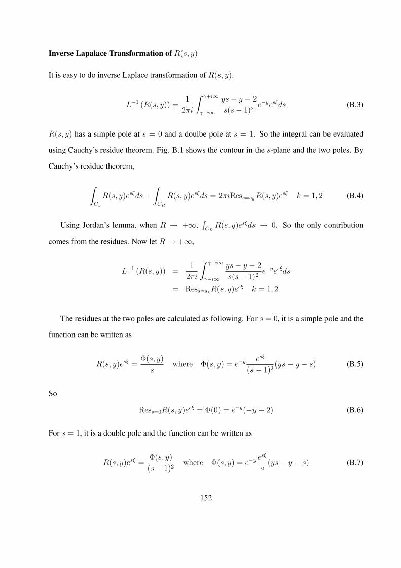
Inverse Lapalace Transformation of R(s, y)
It is easy to do inverse Laplace transformation of R(s, y).
L−1 (R(s, y)) =1
2πi
∫ γ+i∞
γ−i∞
ys− y − 2
s(s− 1)2e−yesξds (B.3)
R(s, y) has a simple pole at s = 0 and a doulbe pole at s = 1. So the integral can be evaluated
using Cauchy’s residue theorem. Fig. B.1 shows the contour in the s-plane and the two poles. By
Cauchy’s residue theorem,
∫
C1
R(s, y)esξds +
∫
CR
R(s, y)esξds = 2πiRess=skR(s, y)esξ k = 1, 2 (B.4)
Using Jordan’s lemma, when R → +∞,∫
CRR(s, y)esξds → 0. So the only contribution
comes from the residues. Now let R → +∞,
L−1 (R(s, y)) =1
2πi
∫ γ+i∞
γ−i∞
ys− y − 2
s(s− 1)2e−yesξds
= Ress=skR(s, y)esξ k = 1, 2
The residues at the two poles are calculated as following. For s = 0, it is a simple pole and the
function can be written as
R(s, y)esξ =Φ(s, y)
swhere Φ(s, y) = e−y esξ
(s− 1)2(ys− y − s) (B.5)
So
Ress=0R(s, y)esξ = Φ(0) = e−y(−y − 2) (B.6)
For s = 1, it is a double pole and the function can be written as
R(s, y)esξ =Φ(s, y)
(s− 1)2where Φ(s, y) = e−y esξ
s(ys− y − s) (B.7)
152

So
Ress=1R(s, y)esξ =Φ′(1)
1!(B.8)
= e−y esξ(2 + y − 2sξ − syξ + s2yξ)
s2|s=1 (B.9)
= e−yeξ(2 + y − 2ξ) (B.10)
Combine the previous results, then
L−1 (R(s, y)) = e−y[−2− y + eξ(2 + y − 2ξ)
](B.11)
1 Re
Im
R
C1
CR
0
Figure B.1: Contour Integration Path around Two Poles for R(s, y)
153

Inverse Laplace Transformation of V (s, y)
The inverse Laplace transformation of V(s,y) is relatively complicated comparing to that of R(s, y)
since it involes the branch cut in the complex domain. R(s, y) has a simple pole at s = 0 and a
double pole at s = 1.It also needs to choose a branch cut for√
s. For simplication, the branch cut
is as the negative real axis. Fig. B.2 shows the contour and the branch cut.
1
Branch
CutRe
Im
R
C1
CR1
CR2
L1
L2
C
Figure B.2: Contour Integration Path around Two Poles and Branch Cut for V (s, y)
According to Cauchy’s residue theorem, the contour integration becomes
∫
C1
+
∫
CR1
+
∫
L1
+
∫
Cρ
+
∫
L2
+
∫
CR2
= 2πiRess=skR(s, y)esξ k = 1, 2 (B.12)
Using Jordan’s lemma, when R → +∞,∫
CR1→ 0 and
∫CR2
→ 0. Now let’s consider the
paths of L1 and L2. On the complex plan, the complex number can be expressed as s = reiθ,
154

where r is the modulus and θ is the argument. Let
f(s, y) = V (s, y)esξ =2
s(s− 1)2esξ−√sy =
2
s(s− 1)2e[
12(ln r+iθ)] (B.13)
On L1, θ = π, s = reiπ:
f(s, y) =2
−r(r + 1)2e−rξ−i
√ry (B.14)
On L2, θ = −π, s = re−iπ:
f(s, y) =2
−r(r + 1)2e−rξ+i
√ry (B.15)
Then
∫
L1
=
∫ ρ
R
− 2
r(r + 1)2e−rξ−i
√rydr (B.16)
=
∫ R
ρ
2
r(r + 1)2e−rξ−i
√rydr (B.17)
=
∫ R
ρ
2
r(r + 1)2e−rξ
[cos (
√ry)− i sin (
√ry)
]dr (B.18)
∫
L2
=
∫ R
ρ
− 2
r(r + 1)2e−rξ+i
√rydr (B.19)
=
∫ R
ρ
− 2
r(r + 1)2e−rξ
[cos (
√ry) + i sin (
√ry)
]dr (B.20)
So, when ρ → 0 and R → +∞
∫
L1
+
∫
L2
= −4i
∫ +∞
0
e−rξ
r(r + 1)2sin (
√ry)dr (B.21)
and when ρ → 0, the integration along the path Cρ can also be evaluated using the Cauchy’s
residue theorem. The residue at s = 0 is calculated as following. The function f(s) can be written
155

as
f(s) =Φ(s)
swhere Φ(s) =
2
(s− 1)2esξ−√sy (B.22)
So
Ress=0 = Φ(0) = 2 (B.23)
Then ∫
Cρ
= −2πiRess=0 = −4πi (B.24)
The residue at s = 1 is calculated as following. Since s = 1 is a double pole, the function f(s)
can be written as
f(s) =Φ(s)
(s− 1)2where Φ(s) =
2
sesξ−√sy (B.25)
So
Ress=1 =Φ′(1)
1!= −e−y+ξ(2 + y − 2ξ) (B.26)
Put all the terms together and after some manupilation, the inverse Laplace transformation of
V (s, y) can be written as
L−1(V (s, y)) = 2− e−y+ξ(2 + y − 2ξ)− 2
π
∫ ∞
0
e−rξ
r(r + 1)2sin (
√ry)dr (B.27)
The final solution for P (y, ξ) has the form
P (y, ξ) = L−1(R(s, y)) + L−1(V (s, y)) (B.28)
= 2
[1−
(y
2+ 1
)e−y − 1
π
∫ ∞
0
e−rξ
r(r + 1)2sin√
rydr
](B.29)
which is the same as in Jeng et al. (2007). When time goes to infinity, the integral in equation
5.37 goes to zero since e−rξ will be infinitesimally small. The final steady state solution is just the
first part of equation 5.37 which is exactly the same as equation 5.36. The steady solution is plotted
in Fig. B.3. The excessive pore pressure at the bed surface is always zero and the the excessive
156

pore pressure at infinite depth is 2.
25
20
15
10
5
00.0 0.5 1.0 1.5 2.0 2.5
Excessive Pore Pressure P
Dep
th y
Steady State
Figure B.3: Steady State Solution of the Excessive Pore Pressure for Deep Soil
157

References
A. Aliabadi, J. Abedi, B. Zellars, K. Bota, and A. Johnson. Simulation technique for wave gener-ation. Communications in Numerical Methods in Engineering, 19:349–359, 2003.
K. Anastasiou and C. Chan. Solution of the 2d shallow water equations using the finite volumemethod on unstructured triangular meshes. International Journal for Numerical Methods inFluids, 24:1225–1245, 1997.
E. Anderson, Z. Bai, C. Bischof, S. Blackford, J. Demmel, J. Dongarra, J. D. Croz, A. Greenbaum,S. Hammarling, A. McKenney, and D. Sorensen. LAPACK User’s Guide. SIAM, Philadelphia,PA., 3 edition, 1999.
F. V. Beek and H. Wind. Numerical modeling of erosion and sedimentation around offshorepipelines. Coastal Engineering, 14:107–128, 1990.
R. Bennett and R. Dolan. Mine burial assessment. state of the art and science, technology, andmodeling. Technical Report Technical Rep. No. SI-0099-05, Seaprobe, Inc., USA, 2001.
A. Bermudez and M. Vazquez. Upwind methods for hyperbolic conservtion laws with sourceterms. Computers and Fluids, 23(8):1049–1071, 1994.
M. Biot. General theory of three-dimensional consolidation. Journal of Applied Physics, 12(2):155–164, 1941.
H. Breusers and A. Raudkivi. Scouring. IAHR Hydraulic Design Manual 2., A.A. Balkemn,Rotterdam, The Netherlands, 1991.
H. Breusers, G. Nicollet, and H. Shen. Local scour around cylindrical piers. Journal of HydraulicResearch, 15(3):211–252, 1977.
B. Brørs. Numerical modeling of flow and scour at pipelines. Journal of Hydraulic Engineering,125(5):511–523, 1999.
Z. Cao, R. Day, and S. Egashira. Coupled and decoupled numerical modeling of flow and morpho-logical evolution in alluvial rivers. Journal of Hydrauic Engineering, 128(3):306–321, 2002.
M. B. Cardenas and J. L. Wilson. Hydrodynamics of coupled flow above and below a sediment-water interface with triangular bedforms. Advances in Water Resources, 30:301–313, 2007.
158

Y. Catano-Lopera. Burial of Short Cylinders Induced by Local Scour and Bedform MigrationUnder Waves Plus Currents. PhD thesis, University of Illinois at Urbana and Champaign, 2005.
A. Chan. User manual for diana-swandyne ii. Department of Civil Engineering, University ofBirmingham, 1995.
S. S. Chatterjee and S. N. Ghosh. Submerged horizontal jet over erodible bed. Journal of theHydraulic Division, 106(HY11):53–90, 1980.
S. S. Chatterjee, S. N. Ghosh, and M. Chatterjee. Local scour due to submerged horizontal jet.Journal of Hydraulic Engineering, 120(8):53–90, 1994.
L. Cheng, B. M. Sumer, and J. Fredsøe. Solutions of pore pressure buildup due to progressivewaves. International Journal of Numerical and Analytical Methods in Geomechanics, 25(9):885–907, 2001.
E. C. Clukey, F. H. Kulhawy, and P. L. F. Liu. Laboratory and Field Investigation of SedimentInteraction, pages 381–396. ASTM STP 883. American Society for Testing and Materials,Philadelphia, 1985.
Y. Cui and G. Parker. Linear analysis of coupled equations for sediment transport. In Environmen-tal and Coastal Hydraulics: Protecting the Aquatic Habitat - Proceedings of Theme B of theXXVII IAHR Congress, pages 1256–1261, San Francisco, 1997.
Y. Cui, G. Parker, E. Thomas, E. James, and M. Annjanette. More on the evolution of bed materialwaves in alluvial rivers. Earth Surface Processes and Landforms, 30:107–114, 2005.
M. Darwish and F. Moukalled. Tvd schemes for unstructured grids. International Journal of Heatand Mass Transfer, 46:599–611, 2003.
P. De Alba, H. B. Seed, and C. K. Chan. Sand liquefaction in large-scale simple shear tests. Journalof Geotechnical Division, ASCE, 103:909–928, 1976.
R. G. Dean and R. A. Dalrymple. Water Wave Mechanics For Engineers and Scientists. WorldScientific, 1991.
I. Demirdzic, S. Muzaferija, and M. Peric. Finite volume method for stress analysis in complexdomains. International Journal For Numerical Methods In Engineering, 37:3751–3766, 1994.
I. Demirdzic, S. Muzaferija, and M. Peric. Benchmark solutions of some structural analysis prob-lems using finite-volume method and multigrid acceleration. International Journal For Numer-ical Methods In Engineering, 40:1893–1908, 1997.
H. DeVriend. 2dh mathematical modeling of morphological evolutions in shallow water. CoastalEngineering, 11:1–27, 1987a.
H. DeVriend. Analysis of horizontally two-dimensional morphological evolutions in shallow wa-ter. Journal of Geophysical Research, 92(C4):3877–3893, 1987b.
159

S. Dey. Local scour at piers, part i: A review of development of research. International Journal ofSediment Research, 12(2):23–44, 1997.
J. Duan and S. Nanda. Two-dimensional depth-averaged model simulation of suspended sedimentconcentration distribution in a groyne field. Journal of Hydrology, 327:426–437, 2006.
B. Duc, T. Wenka, and W. Rodi. Numerical modeling of bed deformation in laboratory channel.Journal of Hydraulic Engineering, 130(9):894–904, 2004.
S. Dunn, P. Vun, A. Chan, and J. Damgaard. Numerical modeling of wave-induced liquefactionaournd pipelines. Journal of Waterway, Port, Coastal, and Ocean Engineering, 132(4):276–288,2006.
F. Engelund and J. Fredsøe. A sediment transport model for straight alluvial channels. NordicHydrology, 7:293–306, 1976.
D. Farshi and S. Komaei. Discussion of ”finite volume model for two-dimensional shallow waterflows on unstructured grids”. Journal of Hydraulic Engineering, 131(12):1147–1148, 2005.
M. Foda, J. Hunt, and H. Chou. A nonlinear model for the fluidization of marine mud by waves.Journal of Geophysical Research, 98(C4):7039–7047, 1993.
F. Gao, D. Jeng, and H. Sekiguchi. Numerical study on the interaction between non-linear wave,buried pipeline and non-homogeneous porous seabed. Computers and Geotechincs, 30:535–547, 2003.
M. H. Garcıa. Sedimentation and Erosion Hydraulics, chapter 6, Hydraulic Design Handbook.McGraw-Hill, Inc., 1999.
M. H. Garcıa and G. Parker. Entrainment of bed sediment into suspension. Journal of HydraulicEngineering, 117(4):414–435, 1991.
B. Gatmiri. Response of cross-anisotropic seabed to ocean waves. Journal of Geotechnical Engi-neering, 118(9):1295–1314, 1992.
A. Grass. Sediment transport by waves and currents. Technical Report FL29, SERC LondonCenter for Marine Technology, 1981.
M. T. Heath. Scientific Computing: An Introductory Survey. McGraw-Hill Companies, 1996.
C. W. Hirt and B. D. Nicholls. Volume of fluid (vof) method for dynamics of free boundaries.Journal of Computational Physics, 39(1):201–225, 1981.
J. Hudson and P. Sweby. Formulation for numericall approximating hyperbolic systems governingsediment transport. Journal of Scientific Computing, 19(1-3):225–252, 2003.
J. Hudson and P. Sweby. A high-resolution scheme for the equations governing 2d bed-load sedi-ment transport. International Journal for Numerical Methods in Fluids, 47:1085–1091, 2005.
160
J. Hudson, J. Damgaard, N. Dodd, T. Chesher, and A. Cooper. Numerical approaches for 1dmorphodynamic modelling. Coastal Engineering, 52:691–707, 2005.
R. I. Issa. Solution of the implicitly discretised fluid flow equations by operator-splitting. Journalof Computational Physics, 62(1):40–65, 1986.
H. Jasak. Error Analysis and Estimation for the Finite Volume Method with Application to FluidFlows. PhD thesis, Imperial College of Science, Technology and Medicine, 1996.
H. Jasak and Z. Tukovic. Automatic mesh motion for the unstructured finite volume method.Transactions of FAMENA, 30(6):1–18, 2007.
H. Jasak and H. Weller. Application of the finite volume method and unstructured meshes to linearelasticity. International Journal For Numerical Methods In Engineering, 48:267–287, 2000.
D. Jeng. Wave-indueced liquefaction potential at the tip of a breakwater: An analytical solution.Applied Ocean Research, 18:229–241, 1996.
D. Jeng. Soil response in cross-anisotropic seabed due to standing waves. Journal of Geotechnicaland Geoenvironmental Engineering, 123(1):9–19, 1997.
D. Jeng and J. Hsu. Wave-indueced soil response in a nearly saturated sed-bed of finite thickness.Geotechnique, 46(3):427–440, 1996.
D. S. Jeng and Y. S. Lin. Wave-induced pore pressure around a buried pipeline in gibson soil:Finite element analysis. International Journal for Numerical and Analytical Methods in Ge-omechanics, 23:1559–1578, 1999.
D. S. Jeng and B. R. Seymour. Simplified analytical approximation for pore-water pressure buildupin marine sediments. Journal of Waterway, Port, Coastal, and Ocean Engineering, 133(4):309–312, 2007.
D. S. Jeng, B. R. Seymour, and J. Li. A new approximation for pore pressure accumulationin marine sediment due to water waves. International Journal for Numerical and AnalyticalMethods in Geomechanics, 31(1):53–69, 2007.
B. E. Lauder and D. B. Spalding. The numerical computation of turbulent flows. ComputerMethods in Applied Mechanics and Engineering, 3(2):269–289, 1973.
R. LeVeque. Balancing source terms and flux gradients in high-resolution godunov methods: Thequasi-steady wave-propagation algorithm. Journal of Computational Physics, 146:346–365,1998.
R. W. Lewis and B. A. Schrefler. The Finite Element Method in the Static and Dynamic Deforma-tion and Consolidation of Porous Media. John Wiley & Sons, second edition, 1998.
F. Li and L. Cheng. Prediction of lee-wake scouring of pipelines in currents. Journal of Waterway,Port, Coastal, and Ocean Engineering, 127(2):106–112, 2001.
161
D. Liang, L. Cheng, and F. Li. Numerical modeling of flow and scour below a pipeline in currentspart ii. scour simulation. Coastal Engineering, 52(1):43–62, 2005.
X. Liu and M. Garcıa. Numerical simulation of local scour with free surface and automatic meshdeformation. In Proceedings of World Environmental and Water Resource Congress, Omaha,NE, 2006a.
X. Liu and M. Garcıa. Numerical simulation of sea bed response under waves with coupled solverof biot consolidation equations and free surface water flow. In Proceedings of ISOPE PACOMS,Dalian, China, 2006b.
X. Liu and M. Garcıa. Numerical investigation of seabed respone under waves with free-surfacewater flow. International Journal of Offshore and Polar Engineering, 17(2):97–104, 2007a.
X. Liu and M. Garcıa. Discussion of ”divergence form for bed slope source term in shallow waterequations” by a. valiani and l. begnudelli. Journal of Hydraulic Engineering, accepted, 2007b.
D. Lyn. Unsteady sediment-transport modeling. Journal of Hydrauic Engineering, 113(1):1–15,1987.
D. Lyn and M. Altinakar. St. venant-exner equations for near-critical and transcritical flows. Jour-nal of Hydrauic Engineering, 128(6):579–587, 2002.
O. Madsen. Wave-induced pore pressure and effective stresses in a porous bed. Geotechnique, 28(4):377–393, 1978.
W. Magda. Wave-induced uplift force acting on a submarine buried pipeline: Finite elementformulation and verification of computations. Computers and Geotechincs, 19(1):47–73, 1996.
S. Mayer and P. Madsen. Simulation of breaking waves in the surf zone using a navier-stokesslolver. In International Conference in Coastal Engineering, Sydney, 2000.
S. Mayer, A. Garapon, and L. S. Sorensen. A fractional step method for unsteady free-surface flowwith application to non-linear wave dynamics. International Journal For Numerical Methods inFluids, (28):293–315, 1998.
W. McDougal, Y. Tsai, and P.-F. Liu. Wave-induced pore water pressure accumulation in marinesoils. Journal of Offshore Mechanics and Arctic Engineering, ASME, 111(1):1–11, 1989.
C. Mei and M. Foda. Wave-induced response in a fluid-filled poro-elastic solid with a freesurface—a boundary layer theory. Geophys. J. Roy. Astron. Soc., 66:597–631, 1981.
B. Melville. Pier and abutment scour: Integrated approach. Journal of Hydraulic Engineering,123(2):125–136, 1997.
B. Melville and S. Coleman. Bridge Scour. Water Resources Publications, Fort Collins, Colorado,USA, 2000.
B. Melville and A. Sutherland. Design method for local scour at bridge piers. Journal of HydraulicResearch, 114(10):1210–1226, 1988.
162
T. Mioduszewski and S. Maeno. Experimental study of scouring process and flow behavior aournda spur dike during the surge pass. In Proceedings of the Thirteenth (2003) International Offshoreand Polar Engineering Conference, pages 858–863, Hnolulu, Hawaii, USA, May 2003. ISOPE.
A. Nayfeh. Introduction to Perturbation Techniques. John Wiley & Sons, 1981.
A. A. S. Neyshabouri, A. M. F. Da Silva, and R. Barron. Numerical simulation of scour by a freefalling jet. Journal of Hydraulic Research, 41(5):533–539, 2003.
M. Nujic. Efficient implementation of non-oscillatory schemes for the computation of free-surfaceflows. Jouranl of Hydraulic Research, 33(1):101–111, 1995.
S. Okusa. Wave-induced stesses in unsaturated submarine sediments. Geotechnique, 35(4):517–532, 1985.
N. R. B. Olsen and M. C. Melaaen. Three-dimensional calculation of scour around cylinders.Journal of Hydraulic Engineering, 119(9):1048–1053, 1993.
N. R. B. Olsen and M. C. Melaaen. Three-dimensional numerical flow modeling for estimation ofmaximum local scour depth. Journal of Hydraulic Research, 36(9):579–590, 1999.
OpenCFD. Openfoam: The open source computational fluid dynamics (CFD) toolbox.http:://www.OpenFoam.org (Dec. 10, 2006), 2006.
G. Parker and M. H. Garcıa. River, Coastal and Estuarine Morphodynamics: RCEM 2005. Taylor& Francis Group, 2006.
S. V. Patankar. Numerical Heat Transfer and Fluid Flow. McGraw-Hill, 1981.
N. Rajaratnam. Turbulent Jet. Elsevier Scientific Publishing Company, 1976.
A. Raudkivi. Functional trends of scour at bridge piers. Journal of Hydraulic Engineering, 112(1):1–13, 1986.
J. E. Richardson and V. G. Panchang. Three-dimensional simulation of scour-inducing flow atbridge piers. Journal of Hydraulic Engineering, 124(5):530–540, 1998.
W. Rodi. Turbulence Models and Their Application in Hydraulics - A State of the Art Review.International Association for Hydraulic Research, Delft, Balkema, 3 edition, 1993.
P. Roe. Approximate riemann solvers, parameter vectors and difference schemes. Journal ofComputational Physics, 43:357–372, 1981.
P. Roe. Characteristic based schemes for the euler equations. Ann. Rev. Fluid. Mech, 18:337–365,1986.
B. Rogers, M. Fujihara, and A. Borthwick. Adaptive q-tree godunov-type scheme for shallowwater equations. International Journal for Numerical Methods in Fluids, 35:247–280, 2001.
163

B. Rogers, A. Borthwick, and P. Taylor. Mathematical balancing of flux gradient and source termsprior to using roe’s approximate riemann solver. Journal of Computational Physics, 192:422–451, 2003.
A. Roulund, B. M. Sumer, J. Fredsøe, and J. Michelsen. Numerical and experimental investigationof flow and scour around a circular pile. Journal of Fluid Mechanics, 534:351–401, 2005.
T. Sakai, H. Gotoh, and T. Yamamoto. Block subsidence under pressure and flow. In Proc. 24thConference on Coastal Engineering (ICCE94), pages 23–28, Kobe, Japan, 1994.
H. Seed and J. Booker. Wave-induced pore pressure in relation to ocean floor stability of cohe-sionless soil. Marine Geotechnology, 3(2):123–150, 1978.
H. B. Seed. Evaluation of soil liquefaction effects on level ground during earthquake. In Liq-uefaction Problems in Geotechnical Engineering, pages 1–104. ASCE Annual Convention andExposition, 1976.
H. B. Seed, P. O. Martin, and J. Lysmer. The generation and dissipation of pore water pressure dur-ing soil liquefaction. Technical Report Report EERC 75-26, College of Engineering, Universityof California, Berkeley, California, 1975.
J. A. Sethian. Level Set Methods: Evolving Interfaces in Geometry, Fluid Mechanics, ComputerVision, and Material Science. Cambridge Monographs on Applied and Computational Mathe-matics. Cambridge University Press, 1996.
J. D. Smith and S. McLean. Spatially averaged flow over a wavy surface. Journal of GeophysicalResearch, 83:1735–1746, 1977.
S.Soares-Frazao and Y. Zech. Dam break in channels with 90 bend. Journal of Hydraulic Engi-neering, 128(11):956–968, 2002.
B. M. Sumer and J. Fredsøe. Wave scour around a large verticle circular cylinder. Journal ofWaterway, Port, Coastal and Ocean Engineering, 127(3):125–134, 2001.
B. M. Sumer and J. Fredsøe. The Mechanics of Scour in the Marine Environment. World ScientificPublishing, New Jersey,USA, 2002.
B. M. Sumer, J. Fredsøe, and N. Christiansen. Scour around a vertical pile in waves. Journal ofWaterway, Port, Coastal and Ocean Engineering, 117(1):15–31, 1992.
B. M. Sumer, N. Christiansen, and J. Fredsøe. Influence of cross section on wave scour aroundpiles. Journal of Waterway, Port, Coastal and Ocean Engineering, 119(5):477–495, 1993.
B. M. Sumer, J. Fredsøe, S. Christensen, and M. T. Lind. Sinking/floating of pipelines and otherobjects in liquefied soil under waves. Coastal Engineering, 38:53–90, 1999.
H. A. Taiebat. Three Dimensional Liquefaction Analysis of Offshore Foundations. PhD thesis,University of Sydney, 1999.
164

O. Ubbink and R. I. Issa. A method for capturing sharp fluid interfaces on arbitrary meshes.Journal of Computatonal Physics, 153:26–50, 1999.
A. Valiani and L. Begnudelli. Divergence form for bed slope source term in shallow water equa-tions. Journal of Hydraulic Engineering, 132(7):652–665, 2006.
L. C. van Rijn. Sediment transport, part II: Suspended load transport. Journal of HydrualicEngineering, 110(11):1613–1641, 1984.
H. G. Weller, G. Tabor, H. Jasak, and C. Fureby. A tensorial approach to computational continuummechanics using object-oriented techniques. Computers in Physics, 12(6):620–631, 1998.
Wikipedia. Soil liquefaction — wikipedia, the free encyclopedia, 2007. http://en.wikipedia.org/w/index.php?title=Soil_liquefaction&oldid=164144829 [Online; accessed 16-October-2007].
W. Wu. Depth-averaged two-dimensional numerical modeling of unsteady flow and nonuniformsediment transport in open channels. Journal of Hydraulic Engineering, 130(10):1013–1024,2004.
T. Yamamoto. Wave-induced instability in seabed. In Proc. ASCE Special Conference, CoastalSediments ’77, volume 25, pages 898–913, Charleston, SC, 1977.
T. Yamamoto, H. Koning, H. Sellmeiher, and E. van Hijum. On the response of a poro-elastic bedto water waves. Journal of Fluid Mechanics, 87(1):193–206, 1978.
T. Yoon and S. Kang. Finite volume model for two-dimensional shallow water flows on unstruc-tured grids. Journal of Hydraulic Engineering, 130(7):678–688, 2004.
M. Yuhi and H. Ishida. Simplified solutions for wave-induced response of anisotropic seabed.Journal of Waterway, Port, Coastal, and Ocean Engineering, 18(1):46–50, 2002.
J. Zhou, D. Causon, C. Mingham, and D. Ingram. The surface gradient method for the treatmentof source term in the shallow-water equations. Journal of Computational Physics, 168:1–25,2001.
J. Zhou, D. Causon, D. Ingram, and C. Mingham. Numerical solutions of the shallow waterequations with discontinuous bed topograph. International Journal for Numerical Methods inFluids, 38:769–788, 2002.
O. Zienkiewicz, A. Chan, M. Pastor, B. Schrefler, and T. Shiomi. Computational Geomechanicswith Special Reference to Earthquake Engineering. Wiley, 1999.
165
Author’s Biography
Xiaofeng Liu was born in the Jiangsu province of China in 1977. He graduated from Tsinghua
University in 2000 with a bachelor’s degree in hydraulic engineering. Then he enrolled the grad-
uate school of Peking University, China, where he worked with Professor J.R. Ni on the problem
of dyke break and flooding of the Yellow river. During the graduate study there, he receieved sev-
eral awards incluing Guanghua and Wusi fellowships. He got his master of science degree with
honor from Peking University in 2003. Since then, Xiaofeng moved to to Champaign, Illinois, to
begin his Ph.D. study in the department of civil and environmental engineering. He worked with
professor Marcelo H. Garcıa as a research assistant. His main work is to conduct numerical model
development and simulations. Following the completion of his Ph.D., Xiaofeng will start to work
as a postdoc in the Hydrosystems Lab, UIUC.
166