c© 2007 by Tae-Jin Yoon. All rights reserved.

A PREDICTIVE MODEL OF PROSODY THROUGH GRAMMATICAL INTERFACE:A COMPUTATIONAL APPROACH

BY

TAE-JIN YOON

B.A., University of Seoul, 1998M.A., University of Seoul, 2000

DISSERTATION

Submitted in partial fulfillment of the requirementsfor the degree of Doctor of Philosophy in Linguistics

in the Graduate College of theUniversity of Illinois at Urbana-Champaign, 2007

Urbana, Illinois

Abstract

Speech prosody is manifest in the acoustic signal through the modulation of pitch, loudness,

duration, and source characteristics (voice quality), which combine to encode the prosodic

structure of an utterance. Prosodic structure defines the location of prominent words and

syllables, and the grouping of words into phonological phrases. Prosodic structure, in turn,

relates the phonological form of an utterance to its morphological, syntactic, semantic, and

pragmatic context. The listener’s task in comprehending speech includes decoding prosodic

structure to aid in identifying the morphological, syntactic, semantic, and pragmatic contexts

that comprise the meaning of the utterance.

The research reported in this dissertation focuses on acoustic and perceptual evidence

for prosody in spoken language, and the relationship between prosodic structure and higher

levels of linguistic organization. The study adopts a computational approach that employs

natural language processing tools, machine learning algorithms, and speech and signal pro-

cessing techniques to investigate prosody in speech corpus data. In this study, I show that

prosodic features of an utterance can be reliably predicted from a set of features that en-

code the phonetic, phonological, syntactic and semantic properties of the local context. The

study uncovers new evidence of the acoustic correlates of prosody, including prosodic phrase

juncture and downstepped pitch-accent in American English, in features related to F0, dura-

tion, and intensity. The study also demonstrates in a series of machine learning experiments

that these acoustic features and features from ‘higher’ levels of linguistic organization are

highly correlated with each other, and that very accurate prediction of prosodic structure

can be achieved on the basis of structural linguistic properties and that detection of prosodic

iii

structure can also be made with a high degree of accuracy on the basis of acoustic cues.

This research contributes to our understanding of the interaction between components of

linguistic grammar, in demonstrating the dependencies between phonetics, phonology, syn-

tax and semantics in the encoding of prosody. In addition, my work building on a stochastic

model of prosody prediction has a direct application in the development of speech technolo-

gies that incorporate linguistic models of prosody, including text-to-speech and automatic

speech recognition systems.

iv

To my parents

v

Acknowledgments

Years ago when I embarked on my doctoral study, my advisor Jennifer Cole asked me what

I wanted to study for my doctoral thesis. I replied without reservation or hesitation that

things like intonation and automatic speech recognition seem to be interesting and fun. She

asked me what backgrounds I had. None was my answer. So many remarkable people have

helped me keep my interests in prosody and speech technologies, and above all complete

my dissertation on prosody with computational methodologies that it simply is not possible

to express my warm-hearted gratitude to all of them. Nevertheless, I would like to express

my gratitude to my committee members: Jennifer Cole, Chin Woo Kim, Mark Hasegawa-

Johnson, Richard Sproat and Chilin Shih.

I am very grateful to have Jennifer as my advisor. Over the years, she has supported

and guided me academically, financially, and morally. Whenever I have felt like I need to

talk to somebody, she has always spared hours of time for listening to my half-baked ideas

even in the midst of her busy schedule. I am also very grateful to Chin Woo Kim, who has

offered to me an opportunity to study at Urbana-Champaign, and who has kindly supported

my study over the years in many ways. Mark is such a wonderful teacher and researcher

that his teaching and research have greatly influenced the contents of my dissertation. I am

very fortunate to have Richard Sproat in my dissertation committee. The approaches in

this dissertation would have been only partially implemented if it had not been the exciting

classes such as computational linguistics classes or text-to-speech synthesis class by Richard

Sproat. I am very grateful to Chilin for her suggestions and help I have received. She has

always kindly offered many helps with her expertise knowledge on many aspects on prosody

vi

whenever I have faced difficult huddles and challenges while working on the computational

approach to prosody.

I would like to thank Jennifer, Mark, & Chilin for creating and maintaining such a unique

interdisciplinary environment where linguists and engineers can collaborate in conducting

meaningful and interesting research. My views and skills in the study of linguistics have

been markedly widen and sharpen by the discussion and collaboration with colleagues in

the interdisciplinary prosody and speech recognition group: Ken Chen, Aaron Cohen, Mar-

garet Fleck, Jeung-Yoon Choi, Heejin Kim, Sarah Borys, Xiaodan Zhuang, Eunkyung Lee,

Yoonsook Mo, Jui-Ting Huang, Kyle Gorman, Arthur Kantor.

The community of faculty, students, and visiting scholars in Chambana has provided a

pleasant and stimulating environment. For years of pleasant conversations and hangouts, I

thank James Yoon, Arregi Karlos, Dan Silverman, Elabbas Benmamoun, Zsuzsanna Fagyal,

Hyoung Youb Kim of Korea University, Jungmin Jo, Yong-hun Lee, Jeeyoung Ha, Han-

sook Choi, Jin-Suk Byun, Chongwon Park, Ji-Hye Kim, Ju-Hyeon Hwang, Young-Sun Lee,

Jung Man Park, Hyunju Park, Eugene Chung, Keun-Young Shin, Youngju Choi, Wooseung

Lee, Margaret Russell, Cecilia Ovesdotter Alm, Heidi Lorimer, Aimee Johansen, Yuancheng

Tu, Erica Britt, Hyojin Chi, Hee Youn Cho, Lori Coulter, Indranil Dutta, Andrew Fister,

Matthew Garley, Hahn Koo, Leonard Muaka, Young Il Oh, Young-Sun Lee, Gary Linebaugh,

Hsin-Yi Dora Lu, Liam Moran, Leonard Muaka, Alla Rozovskaya, Soondo Baek, Eunah Kim,

Suyoun Yoon, Churoo Park, Theeraporn Ratitamkul, Vasin Punyakanok, Lisa Pierce, Brent

Henderson, Steve Atwell, Charles La Warre, Steve Winters, Sandeep Phatak, and Youngshin

Chi.

Outside the geographically challenging Urbana-Champaign area, I had the good fortune

to meet a number of good linguists and to seek pieces of advice from them, including Ste-

fanie Shattuck-Hufnagel, Nanette Veilleux, Julia Hirschberg, Marc Swerts, Mary Beckman,

Pauline Welby, Che-Kuang Lin, Joyce McDonough, Jongho Jun, Sahyang Kim, Mi-rah Oh,

and Sun-Ah Jun.

vii

I also express my heartfelt gratitude to my teachers in Korea: Sahng-Soon Yim, Hoi

Jin Kim and Jong-Sung Lim, whom I thank for their encouragements and support over the

years. Talks with them over the phone across the pacific have always kept me going ahead

with my study. I also express my gratitude to Seok-Chae Rhee, In-han Jun, Young-In Moon,

and Jookyung Lee.

Finally but most importantly, I owe the most to my family in Korea for their unfailing

support and confidence in me. I might not have completed my graduate study if it had

not been for the unfaltering encouragement and support I have received from my parents,

brother, aunts, and sister-in-law.

The research for this dissertation was funded in part by the Beckman Institute for Ad-

vanced Science and Technology through Beckman CS/AI summer fellowships (2004, 2005), a

Beckman Graduate Fellowship (2006), and University of Illinois at Urbana-Champaign (Crit-

icial Research Initiative) through a grant to Mark Hasegawa-Johnson and Jennifer Cole for

the project “Prosody in Speech Recognition,” and the National Science Foundation through

a grant (IIS-0414117) to Mark Hasegawa-Johnson, Jennifer Cole, and Chilin Shih for the

project “Prosody, Voice Quality, and Automatic Speech Recognition.”

viii

Table of Contents

List of Tables . . . . . . . . . . . . . . . . . . . . . . . . . . . . . . . . . . . . xi

List of Figures . . . . . . . . . . . . . . . . . . . . . . . . . . . . . . . . . . . . xiv

Chapter 1 Introduction . . . . . . . . . . . . . . . . . . . . . . . . . . . . . 11.1 Introduction . . . . . . . . . . . . . . . . . . . . . . . . . . . . . . . . . . . . 11.2 Research Question . . . . . . . . . . . . . . . . . . . . . . . . . . . . . . . . 21.3 Methodology . . . . . . . . . . . . . . . . . . . . . . . . . . . . . . . . . . . 31.4 A Prosody Model . . . . . . . . . . . . . . . . . . . . . . . . . . . . . . . . . 41.5 Contribution of the Dissertation . . . . . . . . . . . . . . . . . . . . . . . . . 71.6 Outline of the Dissertation . . . . . . . . . . . . . . . . . . . . . . . . . . . . 8

Chapter 2 A Linguistic Model of Prosodic Structure . . . . . . . . . . . . 122.1 Introduction . . . . . . . . . . . . . . . . . . . . . . . . . . . . . . . . . . . . 122.2 The ToBI (Tones and Break Indices) System of Prosody . . . . . . . . . . . 132.3 A Prosodically Labeled Database . . . . . . . . . . . . . . . . . . . . . . . . 23

2.3.1 Frequency . . . . . . . . . . . . . . . . . . . . . . . . . . . . . . . . . 242.3.2 Reliability of the prosodic labels . . . . . . . . . . . . . . . . . . . . . 262.3.3 Speaker consistency of prosodic realization . . . . . . . . . . . . . . . 29

2.4 Conclusion . . . . . . . . . . . . . . . . . . . . . . . . . . . . . . . . . . . . . 37

Chapter 3 Machine Learning and its Applications to Prosody Modeling 383.1 Introduction . . . . . . . . . . . . . . . . . . . . . . . . . . . . . . . . . . . . 383.2 Machine Learning . . . . . . . . . . . . . . . . . . . . . . . . . . . . . . . . . 39

3.2.1 Memory-based learning (MBL) . . . . . . . . . . . . . . . . . . . . . 413.2.2 Classification and regression tree (CART) . . . . . . . . . . . . . . . 45

3.3 Evaluation Metric . . . . . . . . . . . . . . . . . . . . . . . . . . . . . . . . . 503.3.1 Baselines . . . . . . . . . . . . . . . . . . . . . . . . . . . . . . . . . . 503.3.2 Evaluation Metric . . . . . . . . . . . . . . . . . . . . . . . . . . . . . 50

3.4 Earlier Modeling . . . . . . . . . . . . . . . . . . . . . . . . . . . . . . . . . 533.4.1 Prosodic phrasing prediction . . . . . . . . . . . . . . . . . . . . . . . 543.4.2 Prosodic prominence prediction . . . . . . . . . . . . . . . . . . . . . 59

3.5 Conclusion . . . . . . . . . . . . . . . . . . . . . . . . . . . . . . . . . . . . . 63

ix

Chapter 4 Predictive Models of Prosody through Grammatical Interface 654.1 Introduction . . . . . . . . . . . . . . . . . . . . . . . . . . . . . . . . . . . . 654.2 Feature Extraction . . . . . . . . . . . . . . . . . . . . . . . . . . . . . . . . 66

4.2.1 Syntactic features . . . . . . . . . . . . . . . . . . . . . . . . . . . . . 664.2.2 Phonological features . . . . . . . . . . . . . . . . . . . . . . . . . . . 714.2.3 Semantic features . . . . . . . . . . . . . . . . . . . . . . . . . . . . . 74

4.3 Integration of the Extracted Features . . . . . . . . . . . . . . . . . . . . . . 784.4 Experimental Results . . . . . . . . . . . . . . . . . . . . . . . . . . . . . . . 79

4.4.1 Prosodic phrasing prediction . . . . . . . . . . . . . . . . . . . . . . . 814.4.2 Prosodic prominence prediction . . . . . . . . . . . . . . . . . . . . . 86

4.5 Discussion and Conclusion . . . . . . . . . . . . . . . . . . . . . . . . . . . . 90

Chapter 5 Integrative Models of Prosody Prediction . . . . . . . . . . . . 935.1 Introduction . . . . . . . . . . . . . . . . . . . . . . . . . . . . . . . . . . . . 935.2 Extraction of Acoustic Features . . . . . . . . . . . . . . . . . . . . . . . . . 94

5.2.1 F0 . . . . . . . . . . . . . . . . . . . . . . . . . . . . . . . . . . . . . 945.2.2 Duration . . . . . . . . . . . . . . . . . . . . . . . . . . . . . . . . . . 985.2.3 Intensity . . . . . . . . . . . . . . . . . . . . . . . . . . . . . . . . . . 100

5.3 Integrative Predictive Model of Prosodic Prominence . . . . . . . . . . . . . 1015.3.1 Prediction of the pitch accents using acoustic features . . . . . . . . . 1015.3.2 Prediction of pitch accents using integrative features . . . . . . . . . 104

5.4 Integrative Predictive Model of Prosodic Boundary . . . . . . . . . . . . . . 1095.5 Discussion and Conclusion . . . . . . . . . . . . . . . . . . . . . . . . . . . . 113

Chapter 6 Acoustic Correlates of Prosodic Structure . . . . . . . . . . . . 1186.1 Introduction . . . . . . . . . . . . . . . . . . . . . . . . . . . . . . . . . . . . 1186.2 Acoustic Cues to Layered Prosodic Domains . . . . . . . . . . . . . . . . . . 118

6.2.1 Acoustic cues for prosodic boundary . . . . . . . . . . . . . . . . . . 1206.2.2 Methods . . . . . . . . . . . . . . . . . . . . . . . . . . . . . . . . . . 1236.2.3 Results . . . . . . . . . . . . . . . . . . . . . . . . . . . . . . . . . . . 1246.2.4 Conclusion . . . . . . . . . . . . . . . . . . . . . . . . . . . . . . . . . 130

6.3 Downstepped Pitch Accents . . . . . . . . . . . . . . . . . . . . . . . . . . . 1316.3.1 Introduction . . . . . . . . . . . . . . . . . . . . . . . . . . . . . . . . 1316.3.2 Categorical status of !H* . . . . . . . . . . . . . . . . . . . . . . . . . 1356.3.3 Regression analysis and classification experiment . . . . . . . . . . . . 137

6.4 Discussion and Conclusion . . . . . . . . . . . . . . . . . . . . . . . . . . . . 143

Chapter 7 Conclusion . . . . . . . . . . . . . . . . . . . . . . . . . . . . . . 1457.1 Summary . . . . . . . . . . . . . . . . . . . . . . . . . . . . . . . . . . . . . 1457.2 Conclusion . . . . . . . . . . . . . . . . . . . . . . . . . . . . . . . . . . . . . 147

References . . . . . . . . . . . . . . . . . . . . . . . . . . . . . . . . . . . . . . 148

Vita . . . . . . . . . . . . . . . . . . . . . . . . . . . . . . . . . . . . . . . . . . 160

x

List of Tables

2.1 Inventory of pitch accent in the ToBI system . . . . . . . . . . . . . . . . . . 152.2 Inventory of phrasal tones (either ip or IP) in the ToBI system . . . . . . . . 152.3 Distribution of pitch accents in the radio speech corpus . . . . . . . . . . . . 252.4 Distribution of phrasal tones (i.e., intermediate and intonational phrase) in

the radio speech corpus . . . . . . . . . . . . . . . . . . . . . . . . . . . . . . 252.5 The amount of speech used for transcriber agreement study by Dilley, Breen,

Gibson, Bolivar, & Kraemer (2006) . . . . . . . . . . . . . . . . . . . . . . . 282.6 ToBI labeling of the phrase ‘Massachusetts may now . . . ’ . . . . . . . . . . . 302.7 ToBI labeling of the phrase ‘. . . of the Massachusetts Bar Association . . . ’ . . 302.8 An example of aligning word-prosody pair for a pair of speakers (Female 1

and Male 2) . . . . . . . . . . . . . . . . . . . . . . . . . . . . . . . . . . . . 332.9 Rate of consistency on the presence or absence of pitch accent for each pair

of speakers . . . . . . . . . . . . . . . . . . . . . . . . . . . . . . . . . . . . . 342.10 Rate of consistency on the presence/absence of prosodic boundary for a pair

of speakers . . . . . . . . . . . . . . . . . . . . . . . . . . . . . . . . . . . . . 352.11 Rate of consistency on the types of pitch accent for each pair of speakers . . 352.12 Rate of consistency on the levels of prosodic boundary for each pair of speakers 36

3.1 Illustration of k-nearest neighbor . . . . . . . . . . . . . . . . . . . . . . . . 423.2 A schematic diagram of confusion matrix . . . . . . . . . . . . . . . . . . . . 513.3 Experimental Results of Cohen (2004) on prosodic boundary prediction . . . 563.4 Confusion matrix that shows the results of types of prosodic boundary in Ross

& Ostendorf (1996) . . . . . . . . . . . . . . . . . . . . . . . . . . . . . . . . 583.5 Results of Cohen (2004) on pitch accent prediction using features obtained

from full Charniak parser data . . . . . . . . . . . . . . . . . . . . . . . . . . 603.6 Results of pitch accent type prediction in Ross & Ostendorf (1996) . . . . . . 623.7 Results of pitch accent prediction using both acoustic and text features with

AdaBoost CART in Sun (2002) . . . . . . . . . . . . . . . . . . . . . . . . . 633.8 Results of pitch accent prediction using text features with AdaBoost CART

in Sun (2002) . . . . . . . . . . . . . . . . . . . . . . . . . . . . . . . . . . . 64

4.1 Penn Treebank II part of speech tags . . . . . . . . . . . . . . . . . . . . . . 684.2 Distribution of Parts of Speech in the radio news speech corpus . . . . . . . 694.3 Distribution of shallow syntactic chunks in the radio speech corpus . . . . . 714.4 Distribution of chunking size of the shallow parser in the corpus . . . . . . . 71

xi

4.5 Distribution of phonological word lengths in the corpus . . . . . . . . . . . . 734.6 Distribution of number of syllables in the corpus . . . . . . . . . . . . . . . . 734.7 Distribution of position of lexical stress within the syllable in the corpus . . 734.8 Distribution of grammatical roles in the corpus . . . . . . . . . . . . . . . . 764.9 Distribution of named entities in the corpus . . . . . . . . . . . . . . . . . . 774.10 Distribution of the location of a word within the brackets to which the word

comprising the named entity belongs . . . . . . . . . . . . . . . . . . . . . . 774.11 Representation of features in a matrix format . . . . . . . . . . . . . . . . . 794.12 Confusion matrix of presence or absence of boundary tone . . . . . . . . . . 814.13 Evaluation of presence or absence of boundary tone. . . . . . . . . . . . . . . 814.14 Overall comparison of the presence or absence of prosodic boundary . . . . . 824.15 Information gained under the condition of no pitch accent information, and

with contextual information from a three-word window . . . . . . . . . . . . 834.16 Confusion matrix of strength of prosodic phrase boundary . . . . . . . . . . 844.17 Evaluation of the strength of prosodic phrase boundary . . . . . . . . . . . . 844.18 Overall comparison of predicting the strength of prosodic boundary . . . . . 844.19 Confusion matrix of the type of boundary tones . . . . . . . . . . . . . . . . 854.20 Evaluation of the type of boundary tones . . . . . . . . . . . . . . . . . . . . 854.21 Overall comparison of predicting types of boundary tone . . . . . . . . . . . 864.22 Confusion matrix of presence or absence of pitch accent. TiMBL learner

observing features from a three-word window. . . . . . . . . . . . . . . . . . 864.23 Evaluation of presence or absence of pitch accent. TiMBL learner observing

features from a three-word window. . . . . . . . . . . . . . . . . . . . . . . . 874.24 Overall comparison of the presence or absence of pitch accent . . . . . . . . 874.25 Information gained under the condition of no prosodic boundary information,

and with contextual information from a three-word window . . . . . . . . . . 884.26 Confusion matrix of accent type prediction . . . . . . . . . . . . . . . . . . . 894.27 Evaluation of the type of pitch accents . . . . . . . . . . . . . . . . . . . . . 894.28 Overall comparison of predicting types of pitch accent . . . . . . . . . . . . . 894.29 The comparison of observed and predicted types of pitch accents and bound-

ary tones . . . . . . . . . . . . . . . . . . . . . . . . . . . . . . . . . . . . . . 90

5.1 Prediction of presence/absence of pitch accents using the third order polyno-mial coefficients . . . . . . . . . . . . . . . . . . . . . . . . . . . . . . . . . . 102

5.2 Confusion matrix for predicting the presence or absence of pitch accent usingall the acoustic features . . . . . . . . . . . . . . . . . . . . . . . . . . . . . . 103

5.3 Confusion Matrix on the task of predicting the presence or absence of pitchaccent using both linguistic and acoustic features under the best parametersetting . . . . . . . . . . . . . . . . . . . . . . . . . . . . . . . . . . . . . . . 108

5.4 Confusion matrix for the task of predicting types of pitch accents . . . . . . 1095.5 Confusion matrix of strength of boundary tone using acoustic features using

features related to duration only . . . . . . . . . . . . . . . . . . . . . . . . . 1115.6 Confusion matrix on the task of predicting prosodic boundary using both

linguistic and acoustic features under the best parameter setting . . . . . . . 112

xii

5.7 Confusion matrix of strength of boundary tone using both linguistic andacoustic features . . . . . . . . . . . . . . . . . . . . . . . . . . . . . . . . . 113

5.8 Confusion matrix for the type of boundary tones . . . . . . . . . . . . . . . . 1145.9 Comparison of the presence/absence of pitch accent and prosodic boundary . 116

6.1 Contingency table of the presence/absence of silent pause and the presence/absence of phrasal tone . . . . . . . . . . . . . . . . . . . . . . . . . . . . . . 121

6.2 Frequency table of vowels occurring at word-final syllable . . . . . . . . . . . 1246.3 Frequency table of vowels occurring at word-final syllable under the condition

of the location of lexical stress (penult stress and final stress) . . . . . . . . . 1266.4 Partitioning of the pitch peak values of the first pitch accent . . . . . . . . . 1396.5 Welch two sample t’-test . . . . . . . . . . . . . . . . . . . . . . . . . . . . . 1396.6 Confusion matrix of predicting H* and !H* from the Boston Radio Speech

corpus . . . . . . . . . . . . . . . . . . . . . . . . . . . . . . . . . . . . . . . 142

xiii

List of Figures

1.1 An illustration of a ToBI transcription in the news corpus. . . . . . . . . . . 6

2.1 Illustration of four possible boundary shapes that are made out of one of thephrase accents and one of the boundary tones . . . . . . . . . . . . . . . . . 17

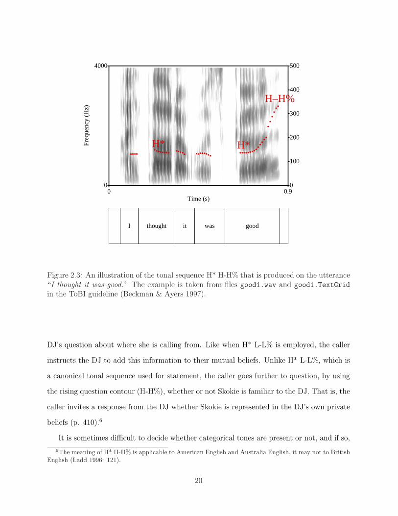
2.2 An illustration of downstepped pitch accents . . . . . . . . . . . . . . . . . . 192.3 An illustration of the tonal sequence H* H-H% that is produced on the utter-

ance “I thought it was good.” The example is taken from files good1.wav andgood1.TextGrid in the ToBI guideline (Beckman & Ayers 1997). . . . . . . 20

2.4 Overlapped F0 contours of the phrase “Massachusetts may now . . . ” . . . . . 302.5 Overlapped F0 contours of the phrase “. . . of the Massachusetts Bar Associ-

ation . . . ” . . . . . . . . . . . . . . . . . . . . . . . . . . . . . . . . . . . . . 31

3.1 An Example of CART Representation of Intonation Phrase Prediction . . . . 473.2 An Example of CART Representation of Pitch Accent Prediction . . . . . . 493.3 Correlation of F-Value . . . . . . . . . . . . . . . . . . . . . . . . . . . . . . 53

5.1 Raw pitch contour . . . . . . . . . . . . . . . . . . . . . . . . . . . . . . . . 955.2 Post-processed pitch contour using linear interpolation and median filtering

with the window of 11 pitch . . . . . . . . . . . . . . . . . . . . . . . . . . . 965.3 Mean and standard deviation of duration of each vowel in the Boston Univer-

sity Radio Speech Corpus . . . . . . . . . . . . . . . . . . . . . . . . . . . . 995.4 Overall progress of exhaustive parameter search that aims to find the best

setting of the parameters . . . . . . . . . . . . . . . . . . . . . . . . . . . . . 1065.5 Average normalized rime duration of each phone type . . . . . . . . . . . . . 1105.6 Overall progress of exhaustive parameter search that results in the best setting

for the boundary location prediction . . . . . . . . . . . . . . . . . . . . . . 112

6.1 An illustration of two levels of prosodic boundary. . . . . . . . . . . . . . . . 1196.2 An example that illustrates low-toned ip (L-) and low-toned IP (L-L%), taken

from the Boston University Radio Speech Corpus. Two instances of L- ob-served on words “Hennessy” and “act” are not necessarily followed by anyaudible silent pause. . . . . . . . . . . . . . . . . . . . . . . . . . . . . . . . 121

6.3 Measurement domain for normalized duration . . . . . . . . . . . . . . . . . 1256.4 Schematic diagram of the two locations of word-level stress for words in the

present study. . . . . . . . . . . . . . . . . . . . . . . . . . . . . . . . . . . . 125

xiv

6.5 Effect of prosodic boundary on final nucleus duration (final stress) . . . . . . 1276.6 Effect of pitch accent on final nucleus duration (final stress) . . . . . . . . . 1286.7 Effect of prosodic boundary on final nucleus duration (penult stress) . . . . . 1296.8 Effect of accent-induced lengthening on final nucleus duration (penult stress) 1306.9 An illustration of downstepped pitch accent observed in the Boston University

Radio Speech corpus. . . . . . . . . . . . . . . . . . . . . . . . . . . . . . . . 1326.10 Hypothetical bimodal distribution . . . . . . . . . . . . . . . . . . . . . . . . 1346.11 Pitch drop measure defines a uni-modal distribution . . . . . . . . . . . . . . 1356.12 Scatterplot of H*H* versus H*!H* in the Boston Radio Speech corpus . . . . 1386.13 Box plot of H* and !H* (I) . . . . . . . . . . . . . . . . . . . . . . . . . . . . 1406.14 Box plot of H* and !H* (II) . . . . . . . . . . . . . . . . . . . . . . . . . . . 141

xv

Chapter 1

Introduction

1.1 Introduction

Language is a cognitive function unique to humans, and among humans with unimpaired

speech and hearing, linguistic activity is manifest primarily in speech. Speech is produced by

the systematic coordination of articulatory gestures, and conveys linguistic information at

many levels. Speech sounds are sequenced to form words, words are grouped into syntactic

phrases and sentences, and sentences are combined to construct discourse. Information at

each of these levels is communicated through the shared medium of the speech signal, and

the listener is faced with the complex task of decoding the signal to uncover the elements of

meaning at each level.

The intonation and rhythm of speech play an important role in expressing meaning.

These properties in an utterance reflect the prosodic structure of the language, which can be

utilized in conveying syntactic information (about the grouping of words into syntactic con-

stituents), as well as pragmatic information (identifying the focal words in an utterance, and

encoding the speech act as a declaration, a question, etc.). For example, a sentence like “I

saw the boy with a telescope” is ambiguous in written form. It can mean either (i) “I saw the

boy who had a telescope” or (ii) “I saw the boy with the aid of a telescope.” Prosodic struc-

ture can disambiguate this sentence, through the grouping of words in prosodic phrases: (I

saw) (the boy with a telescope) for (i) or (I saw the boy) (with a telescope) for (ii).1 Prosodic

1Many earlier studies show that under certain circumstances listeners use the prosodic organization of anutterance to guide their interpretation of a phrase that has a structural ambiguity (e.g., Price, Ostendorf,Shattuck-Hufnagel & Fong 1991; Kjelgaard & Speer 1999; Snedeker & Trueswell 2003, among others.).

1

structure is crucial in conveying pragmatic information, too.2 Depending on the discourse

context, a sentence like “My car broke down.” can be spoken with emphasis on down, as “My

car broke DOWN.” as an answer to the question “What happened to your car?” or with em-

phasis on car, as “My CAR broke down.” as an answer to the question “Did your motorcycle

break down?”.3 This kind of information, some of which is conveyed through punctuation

in written languages, is expressed through the modulation of pitch, loudness, duration, and

voice quality across the syllables in an utterance. Investigating prosody through the study

of these acoustic features is complicated by the fact that pitch, loudness, duration and voice

quality are also affected by paralinguistic properties of the utterance (e.g., the speaker’s

emotional state), and even by non-linguistic factors (e.g., speaker’s gender and age).

1.2 Research Question

The prosodic structure of speech is based on complex interactions within and between several

different levels of linguistic and paralinguistic organization, and is expressed in the modula-

tion of fundamental frequency (F0), intensity, duration, and voice quality, and the occurrence

of pauses. There are two dimensions of prosodic structure at levels of the prosodic hierarchy

above the (prosodic) word: phrasal prominence and phrasal juncture. Phrasal prominence

refers to the perceptual salience of a word relative to other words in the same prosodic

phrase, where perceptual salience is enhanced through manipulation of the acoustic dimen-

sions mentioned above. Phrasal juncture is the degree of separation or linkage between words

that encodes the presence or absence, respectively, of a phrase boundary.

My research on prosody addresses two fundamental questions: (i) what are articulatory,

acoustic and/or perceptual cues of categories of prosodic structure? and (ii) what is the re-

lationship between prosodic structure and other dimensions of linguistic structure, including

2Experimental studies on the utilization of prosody in conveying pragmatic information such as newinformation are found, e.g., Dahan, Tanenhaus, & Chambers 2002; Watson, Tanenhaus & Gunlogson 2004;Ito & Speer 2006, among others.

3The example is taken from Lambrecht (1994).

2

phonology, syntax, and semantics? My research is motivated by the fact that even though

substantial progress has been made in modeling prosodic structure based on research from

linguistics, psycholinguistics, and speech technology studies, there remain numerous con-

troversial issues whose resolution will require additional empirical evidence (Cutler, Dahan,

Doneselaar 1997; Ladd 1996; Shattuck-Hufnagel & Turk 1996; Selkirk 2000). As expressed

in Selkirk (2000), “no consensus has emerged within the various traditions of research on

prosodic phrasing concerning the nature of the relationship between prosodic phrasing and

other distinct types of grammatical representation (p. 231).” In particular, existing works

combined show that prosodic prominence and phrasing is affected by syntactic structure, ar-

gument structure, information structure, phonological structure, and even prosodic structure

itself, among other linguistic factors. But these works do not fully explain the contribution

these factors make to the determination of prosodic prominence and phrasing, or the inter-

action among factors.

The first goal of this research is to investigate the extent to which acoustic features encode

prosodic prominence and phrasing, and the extent to which linguistic features determine

prosodic prominence and phrasing. The impact of linguistic factors in determining prosodic

structure will be assessed primarily on the basis of perceived prosodic features and their

acoustic correlates identified in speech. The second goal of the research is to investigate

more narrowly the acoustic correlates of those aspects of prosodic structure that are elusive

or controversial.

1.3 Methodology

To achieve the above-stated goals, I employ tools from computational linguistics and meth-

ods of acoustic analysis in utilizing a corpus of read-style of radio news speech. By employ-

ing tools from computational linguistics, I extract linguistic features of phonology, syntax,

argument structure and semantic structure from the word transcriptions and dictionary ac-

3

companying the radio news corpus. The advantage of using computational tools or natural

language processing techniques is that it allows the automatic extraction of relevant abstract

linguistic features. In addition to the abstract linguistic features, I also use speech analysis

tools to extract acoustic measures from the speech signals in the radio news corpus.

The automatically extracted acoustic measures and linguistic features are tested for their

role in predicting prosodic structure, using machine learning techniques. The goal of machine

learning experiments is to find generalized patterns in the data, and to use the generalized

patterns on unseen data in a similar task. For example, if the right-edge of a syntactic phrase

is observed to coincide with the right-edge prosodic phrasing to a significant extent, then

machine learning algorithms that encode the right-edge of a syntactic phrase as a feature to

be used in the task of predicting prosodic phrase boundaries in an utterance will learn the

patterns in the data, and apply the learned patterns to unseen data of a similar speech style.

The advantage of applying machine learning is that we can test how far particular features

or combinations of features contribute to the patterning of the data. The overall goal is to

identify which features and feature combinations effectively predict the location of prosodic

events such as phrasal prominence and phrasal juncture.

1.4 A Prosody Model

To apply a machine learning algorithm to predict prosodic events, a large speech database

with labeled prosodic events is required. The Boston University Radio Speech corpus (Os-

tendorf, Price & Shattuck-Hufnagel 1995) is one of the largest corpora with labeled prosodic

events. The prosodic events of phrasal prominence and juncture in the corpus are repre-

sented using the ToBI (Tones and Break Indices) system for American English (Beckman &

Ayers 1997).

The ToBI system is a standard prosodic annotation system, and is a variant of the

prosodic model originally proposed by Pierrehumbert (1980) and subsequently developed

4

together with her colleagues (Beckman & Pierrehumbert 1986, Pierrehumbert & Beckman

1988, Pierrehumbert & Hirschberg 1990).4 In the ToBI system, two kinds of prosodic infor-

mation are encoded: (1) tonal information, and (2) information on the degree of juncture

between words.

In principle, pitch contours can be described either in terms of sequences of level target

tones such as high or low, or as sequences of pitch movements such as falling or rising. The

ToBI model of intonation describes the continuous pitch contour using a sequence of level

target tones.5 Specifically, the series of tonal targets are comprised of the atomic features

of high (H) and low (L) that specify tonal height. For example, a rising pitch contour is

represented with a leading low tone (L) plus a target high tone (H).

The tonal inventory in the ToBI system consists of pitch accents marked with a star *

(e.g., H*, L*), phrase accents (marking intermediate phrase juncture) indicated with a dash

- (e.g., H-, L-), and boundary tones (marking intonational phrase juncture) denoted by a

percent sign % (e.g., H%, L%).6 In addition, there is a downstepped accent, which realizes

a high tone in a compressed pitch range, and which is marked with an exclamation mark !

in front of H (e.g., !H*, !H-).

An example of a ToBI transcription is shown in the 3rd tier in Figure 1.1. The figure

is taken from an utterance “That year Thomas Maffy, now president of the Massachusetts

Bar Association, was Hennessy’s law clerk.” produced by a female speaker in the Boston

University Radio Speech corpus. The utterance is chunked into three parts.

The top tier in Figure 1.1 contains a waveform and the 2nd tier contains a spectrogram

with superimposed F0 contour. The two tiers at the bottom comprise components of the

4See Beckman, Hirschberg, & Shattuck-Hufnagel (2005) for detailed historical and anecdotal account ofhow the intonation model of Pierrehumbert (1980) has evolved into the ToBI system of prosody.

5Two widely known phonological approaches to the description of intonation are ‘movement (or config-uration)’ approach and ‘level’ approach. The ‘movement’ approach to the description of intonation, whichemphasizes the role of pitch movement such as falling or rising, is often associated with the British tradition(e.g. O’Connor & Arnold 1961), and the ‘level’ approach, which describes the pitch movements as a sequenceof two level tones, is often associated with the American tradition (e.g., Pike 1945, Trager & Smith 1951,and Pierrehumbert 1980). See Ladd (1996:59-70) for detailed discussion.

6I will present more detailed description of the ToBI system in Chapter 2.

5

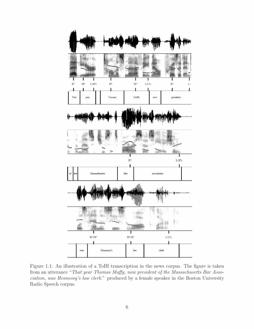
Figure 1.1: An illustration of a ToBI transcription in the news corpus. The figure is takenfrom an utterance “That year Thomas Maffy, now president of the Massachusetts Bar Asso-ciation, was Hennessy’s law clerk.” produced by a female speaker in the Boston UniversityRadio Speech corpus.

6

ToBI system: (1) labels of perceived tonal events (the 3rd tier) and (2) the word transcription

(the 4th tier).

The ToBI transcription system is a perceptual transcription system aided by visual and

auditory inspection of the sound file. In this model, as in the original model of Pierrehumbert

(1980), neither absolute pitch range nor relative excursion size is considered part of the

underlying prosodic representation.

Despite the sparseness of the ToBI system regarding the phonetic realization, there are

a couple of advantages in using the ToBI model over models such as Prosodic Phonology

(Nespor & Vogel 1986). First, the prosodic categories are defined in terms of tone and break

index features, without explicit reference to other grammatical structures such as syntax. As

a consequence, the ToBI system is flexible enough to serve as an interface to other linguistic

components, as exemplified by Steedman (2000) and Pierrehumbert & Hirschberg (1990).

Second, in the years since its introduction studies of linguistic, psycholinguistic and speech

technologies have accumulated evidence in support of the ToBI model in capturing “those

tonal distinctions that are subject to phonological or interpretational constraints (Bartels

1997: 24).”

1.5 Contribution of the Dissertation

The research in this dissertation will make both theoretical and applied contributions to the

study of speech prosody.

On the theoretical level, my research will contribute to a better understanding of how

different grammatical and/or acoustic features interact in forming prosodic prominence and

phrasing. The proposal is expected to address the concern expressed by Ladd (1996), who

states that “in the standard theory, the correspondence between syntactic constituent types

and prosodic ones is highly variable, since the make-up of the prosodic constituents is influ-

enced by a variety of essentially linear factors (p. 334).”

7

On the applied level, my research will inform the development of systems for the au-

tomatic prediction of prosodic categories, which in turn will enable the creation of Text-

To-Speech (TTS) systems with enhanced intelligibility and naturalness. My research will

also facilitate work on prosody detection for use in Automatic Speech Recognition (ASR)

systems. While my research is not directly concerned with improving ASR systems, it can

be viewed as the first step towards the goal of automatically obtaining prosodically-labeled

data as a means of bootstrapping prosodic analysis for ASR. As reflected in Chen (2004),

“the shortage of prosodically transcribed speech data is the biggest obstacle that hinders

our [i.e., prosody-induced ASR, TJY] system from being widely used (p. 105).”

1.6 Outline of the Dissertation

The remainder of this dissertation is structured as follows:

In Chapter 2, I present the prosodic model that serves as the theoretical basis for

my research, along with the speech corpus used for the experiments. I describe in de-

tail the standard prosody annotation system, i.e., the ToBI system, for American English.

Then, I present the Boston University Radio Speech corpus, a large prosodically-transcribed

database that is used throughout in this dissertation. While presenting the radio speech

corpus, I review transcriber reliability studies reported for this corpus, and demonstrate the

speaker variation (or consistency) observed in the corpus.

Chapter 3 presents an overview of a machine learning algorithm and summarizes earlier

studies on the prosodic structure prediction. Probabilistic approaches are more suitable than

deterministic approaches in describing and modeling prosodic structure, due to its variabil-

ity. Machine learning approaches, as one of such probabilistic approaches, possess attractive

characteristics in that a machine learning algorithm finds the underlying generalization of

the data. I review two such algorithms, the memory-based learning (MBL) algorithm and

classification and regression tree (CART). The two algorithms have been successfully and

8

widely used in many research areas including natural language processing as well as prosody

modeling. I turn to the presentation of standard evaluation metrics such as baseline, preci-

sion, recall and accuracy that are typically employed to evaluate the performance of machine

learning algorithms. I conclude the chapter by summarizing earlier studies of prosodic struc-

ture prediction.

Chapter 4 demonstrates the predictive models of prosodic structure through grammatical

interface. I provide a probabilistic model of the mapping between prosody and phonological,

syntactic, and semantic features. The model encodes phonological features, shallow syntac-

tic constituent structure, argument structure, and the status of words as named entities.

A machine learning experiment using these features to predict prosodic phrase boundaries

achieves more than 92% accuracy in predicting prosodic boundary location. The experiment

of predicting prosodic prominence location achieves over 87% accuracy. This study sheds

light on the relationship between prosodic structure and other grammatical structures. But

at the same time, the study reveals some aspects of prosodic structure that are not well un-

derstood and controversial. These aspects are further investigated in the following chapters.

Chapter 5 presents experimental results of predicting prosodic structure through the in-

tegrative set of acoustic and linguistics features derived from both the speech signals and

the grammatical structures. In the previous chapter, I have demonstrated that linguistic

features contribute much to the determination of the prosodic prominence location and the

prosodic boundary location, as evaluated by the high accuracy rates. Prosodic structure

can be approached from different perspectives: On one hand, the prosodic constituents are

investigated based on the syntactic structures of an utterance (Selkirk 1984, Nespor & Vogel

1986, cf. Steedman 2000). The syntax-driven approach seeks to understand the mapping

from syntactic structure to intonational phrasing. On the other hand, the Autosegmental-

Metrical theory of intonational phonology (Pierrehumbert 1980, Beckman & Pierrehumbert

1986), on which the ToBI system is based, investigates prosodic constituents on the basis

of the perceived intonation pattern of an utterance. The phonology/phonetics-driven per-

9

spective seeks to understand the phonological structures that encode prosodic phrasing and

accentuation, and how these structures relate to other aspects of phonological structure (e.g.,

syllable, metrical structure). It is also concerned with the acoustic correlates of intonational

events, as a way of establishing the empirical basis of investigation. In this chapter, I show

that experimental results obtained through the predictive model of prosodic structure, inte-

grating features extracted from grammatical components and the acoustic signal show that

the linguistic features and acoustic cues are highly correlated with each other. The results

lead us to conclude that the prosodic structure can be predicted on the basis of structural

linguistic properties, and detected on the basis of acoustic cues.

Chapter 6 investigates the acoustic correlates of aspects of prosodic structure, concen-

trating on the acoustic correlates of levels of prosodic phrasing (intermediate phrase (ip) vs.

Intonational Phrase (IP)) on the one hand, and the acoustic correlates of downstepped pitch

accent on the other hand. These two aspects of the prosodic structure are not well under-

stood and are controversial, and the machine learning approaches in the previous chapters

are limited in their ability to uncover new evidence. The study reported in this chapter

uncovers new acoustic evidence for the distinction between two levels of prosodic phrase

juncture and for the existence of downstepped pitch-accent. In the first part of the chapter,

I present acoustic evidence from the radio speech corpus for a distinction between levels

of prosodic boundaries. I investigate the phonetic encoding of prosodic structure through

analysis of the acoustic correlates of prosodic boundary and the interaction with phrase

stress (pitch accent) at three levels of prosodic structure: Word, ip, and IP. Evidence for

acoustic effects of prosodic boundary is shown in measures of duration local to the domain-

final rhyme. These findings provide strong evidence for prosodic theory, showing acoustic

correlates of a 3-way distinction in boundary level. In the second part of the chapter, I

present evidence from acoustic analysis and a machine learning experiment for a categori-

cal distinction between non-downstepped and downstepped high-toned pitch accent (H* vs.

!H*). The experimental findings from naturally ocurring speech corpus provide evidence for

10

!H* as a distinct prosodic category.

Chapter 7 concludes the dissertation.

11

Chapter 2

A Linguistic Model of ProsodicStructure

2.1 Introduction

The theory of prosody is a phonological theory of the way in which “the flow of speech is

organized into a finite set of phonological units” (Nespor & Vogel 1986: 299), or the “organi-

zational structure of speech” (Beckman 1996: 21, Shattuck-Hufnagel & Turk 1996: 196). As

such, the phonological grammar of intonational patterns must specify all the relevant tonal

categories, and how the tune (or the pitch pattern) specified in the tonal categories aligns

with the text of an utterance. When one is precise about the prosodic structure assumed,

he/she then can explore “issues in the phonological structures in tandem with other gram-

matical structures” such as syntax or semantics (Beckman 1996: 64). In this dissertation,

I rely on the ToBI (Tones and Break Indices) framework for prosody annotation, which is

based in the autosegmental-metrical theory of phonology (Ladd 1996), focusing mainly on

the categories of prosodic prominence (i.e., pitch accents) and tonally marked phrases at

levels of prosodic hierarchy above the (prosodic) word (i.e., intermediate and intonational

phrases). The ToBI system and its predecessors are just one of many proposed models

of prosody. For a bird’s eye view of various prosody models, see Ladd (1996), Shattuck-

Hufnagel & Turk (1996), Botinis, Granstrom, & Mobius (2001), Sun (2002), Gussenhoven

(2004), Shih (to appear), and references therein.

In what follows, I introduce the ToBI framework of prosody in detail, and then present the

Boston University Radio Speech corpus, which is a corpus of news stories read by professional

radio news announcers, and one of the largest prosodically-labeled corpora. The radio speech

12

corpus includes four different news stories, and is prosodically labeled, and this is the corpus

used for experiments that are conducted and reported in this dissertation. I review the

transcriber reliability studies conducted on this corpus and present my analysis on the rate

of inter-speaker consistency (or in its opposite sense, variation) in the way multiple speakers

realize prosodic events when reading the same scripts.

2.2 The ToBI (Tones and Break Indices) System of

Prosody

The ToBI system of prosody is based on the tonal account of intonation originally proposed

by Pierrehumbert and her colleagues (Pierrehumbert 1980; Liberman & Piterrehumbert

1984; Beckman & Pierrehumbert 1986; Pierrehumbert & Beckman 1988; Pierrehumbert

& Hirschberg 1990) (hence Tones), and the account of degree of juncture between words

proposed in Price, Ostendorf, Shattuck-Hufnagel, & Fong (1991) (hence Break Indices).

ToBI was developed in the 1990’s (Silverman et al. 1992; Beckman & Ayers 1997; see

Beckman, Hirschberg, & Shattuck-Hufnagel 2005), and is a widely used prosody annotation

system.

The ToBI system of prosody shares with its precursor the autosegmental approach to

intonation modeling. The autosegmental approach explicitly separates phonological feature

specification from its phonetic implementation on the one hand, and feature specification

from the segmental string on the other hand (Goldsmith 1976). A defining characteristic of

the autosegmental-based intonation model is the sparseness of its tonal inventory. Only two

levels of tonal target are recognized, H for high tone and L for low tone. Pitch movements

such as falling or rising are analyzed as tone sequence.1 No theoretical postulate is made

regarding a relative pitch range or relative excursion size of the pitch movements.2

1Pitch movements are analyzed as tone sequences.2This is not to say that, for example, listeners are insensitive to pitch range and pitch height. However,

these are assumed to be paralinguistic effects that have not been grammaticalized (Ladd 1990; Terken &

13

Due to the simplicity of the intonation model, the ToBI annotation system is adapted

for other varieties of English, such as Glasgow English (Mayo et al. 1997), and also for other

languages, including German (Grice et al 1996), Japanese (Venditti 1997), Korean (Beckman

& Jun 1996; Jun 1999), Greek (Arvaniti & Baltazani 2005), Serbo-Croatian (Godjevac 1999),

Mandarin (Peng, et al. 1999), Cantonese (Wong, Chan, & Beckman 2005), among others.

The wide-spread use of the ToBI system has paved the way for the study of typological

differences and similarities in prosodic systems across languages (see Jun 2005).3

In the ToBI system, prosodic events are annotated on multiple tiers: a tone tier, an

orthographic tier, a break index tier, and a miscellaneous tier. Additional tier(s) can be

used depending on research needs. The core prosodic events are the events labeled on the

tone and break index tiers (Beckman & Ayers 1997).

On the tone tier are described labels for distinctive pitch events such as pitch accents,

phrase accents, and boundary tones. Pitch accents are marked using a star * at the stressed

syllable in the lexical item (though, not every stressed syllable has a pitch accent). Types of

pitch accent include: a peak accent “H*”, a low accent “L*”, a scooped accent “L*+H”, a

rising peak accent “L+H*”, and a downstepped peak accent “H+!H*”, as described in Table

2.1. The tonal feature not marked * in the bitonal pitch accents is called either the leading

tone (L in case of L+H*) or the trailing tone (H in case of L*+H).

The pitch accents contribute to the determination of discourse meaning. Pierrehumbert

& Hirschberg (1990) develop a compositional model of the interpretation of intonation. They

propose that a pitch accent associates with a lexical item which a speaker intends to make

salient to a hearer. In general, any pitch accent containing H* (e.g., H* and L+H*) associates

with a lexical item which the speaker wants the hearer to perceive as new in the discourse.

Any L* pitch accent (e.g., L*, L*+H) associates with an item which the speaker intends

Hermes 2000).3Because of the various instances of the ToBI system in many languages, a specific instance of the ToBI

system is named with a prefix, such as ‘MAE ToBI’ for the ‘mainstream American English ToBI system,‘K-ToBI’ for the ‘Korean ToBI system’, ‘X-JToBI’ for the ‘extended Japanese ToBI’, etc.

14

Table 2.1: Inventory of pitch accent in the ToBI system

Pitch accent DescriptionH* peak accent Tone target in the upper part of the speaker’s pitch

range for the phraseL* low accent Tone target in the lower part of the speaker’s pitch

rangeL*+H scooped accent Low tone target immediately followed by a relatively

sharp riseL+H* rising peak accent High tone target immediately preceded by a relatively

sharp riseH+!H* downstepped High tone target stepped down from an even higher

peak accent pitch that cannot be accounted for by a preceding Hphrase tone or H pitch accent in the same phrase

to be salient but at the same time does not intend to form part of what the speaker is

predicating in the utterance.

ToBI recognizes two levels of prosodic boundary: intermediate phrase (ip) and intona-

tional phrase (IP). An intermediate phrase tone (also called a phrase accent) is assigned

either a H-, !H- or L- marker at the phrasal right-edge corresponding to a final high, down-

stepped or low tone, respectively. An intonational phrase has a final boundary tone marked

by either L% or H%. Sometimes the intonational phrase begins with relatively high tone,

and is marked by %H. The categories of phrasal tones of ip and IP are in Table 2.2.

Table 2.2: Inventory of phrasal tones (either ip or IP) in the ToBI system

Phrasal tone DescriptionL- !H-, or H- Low, downstepped high, or high tone target occurring at an intermediate

phrase boundaryL% or H% Low or high tone target occurring at an intonational

phrase boundary%H Tonal target relatively high in the speaker’s pitch range

that occurs at the beginning of an intonational phrase

The phrasal tones associate with the end of phrases and utterances. In general, a non-low

15

pitch at a boundary (e.g., H- or H%) indicates non-finality, or the speaker’s intention for the

hearer to interpret what comes after the tone with respect to what has come before. (Pier-

rehumbert & Hirschberg 1990) Intermediate phrases within an utterance may have a final

high (H-) or low (L-) tone and indicate their relationship to a subsequent phrase within the

same utterance. At the intonational phrase level, an utterance of one or more intermediate

phrases ends with a boundary tone, and is indicated by L% or H%. The boundary tone

governs the utterance as a whole, indicating the relationship of the utterance to the subse-

quent utterance. According to Pierrehumbert and Hirschberg, the choice of boundary tone

conveys whether the current intonational phrase is “forward-looking” or not (p. 305). For

example, the boundary tone with H% is interpreted with respect to a succeeding utterance.

Since intonational phrases are composed of one or more intermediate phrases plus a

boundary tone, full intonational phrase boundaries will have two phrasal tones. Four possible

boundary shapes can be made out of one of the phrase accents of either H- or L-, and one

of the boundary tones of either H% or L%, resulting in H-H%, H-L%, L-H%, and L-L%.

Canonical examples of the four boundary tone are illustrated in Figure 2.1. The examples

are taken from the wave and label files available in the ToBI guideline (Beckman & Ayers

1997).4 The wave and label files called money (i.e. money.wav and money.TextGrid) are

used for the graphical representation in Figure 2.1.

The respective meaning of the four boundary tones are as follows (Pierrehumbert &

Hirschberg 1990; Bartels 1997): H-H% is a high rising boundary, indicating that the material

within the utterance requires subsequent discourse for interpretation, by the same speaker

or by the hearer. The interpretation is supported by the fact that the canonical yes-no

question ends with this H-H% boundary tone. L-H% is a low rising boundary, and is called

‘continuation rise,’ indicating that the interpretation within the utterance is to be continued

in the next utterance. H-L% is a plateau boundary, indicating that the material within the

utterance is to be continued or elaborated upon. The pitch contour of this H-L% is rather

4The wave and TextGrid files are available online at http://www.ling.ohio-state.edu/~tobi/ame tobi/

16

Time (s)0.2 1.550

4000

Fre

quen

cy (

Hz)

L* L*

H–H%

0

100

200

300

400

500

Is that Marianna’s money?

Time (s)0.2 1.70

4000

Fre

quen

cy (

Hz)

H* H* L–H%

0

100

200

300

400

500

Is that Marianna’s money?

Time (s)0.25 1.40

4000

Fre

quen

cy (

Hz)

H* H–L%

0

100

200

300

400

500

That’s Marianna’s money

Time (s)2.2 3.50

4000

Fre

quen

cy (

Hz)

H*

L–L%

0

100

200

300

400

500

That’s Marianna’s money

Figure 2.1: Illustration of four possible boundary shapes that are made out of one of thephrase accents (either H- or L-), and one of the boundary tones (either H% or L%). Fromthe top left, the utterances are ToBI-transcribed as: (a) H* H-H%; (b) H* L-H%; (c) H*H-L%; (d) H* L-L%. The wave and label files money.wav and money.TextGrid are used forthe graphical display. The files are available in the ToBI guideline (Beckman & Ayers 1997).

flat, not falling down from a rather high pitch. Finally, L-L% is a falling boundary, indicating

that the material within the utterance concludes a thought or turn. This boundary tone is

most commonly observed at the end of a statement.

17

Downstep is the another prosodic category, and refers to the phonological compression

of a pitch range that lowers a high tone (H*, L+!H*, or H-), as illustrated in Figure 2.2.

In ToBI, downstepped tones are marked explicitly using ‘!’ preceding the downstepped

H pitch accent (i.e., !H* or L+!H*) or the downstepped H phrase accent (i.e., !H-). In

Pierrehumbert’s (1980) system, a bitonal pitch accent such as L+H* is a downstep trigger, as

shown in Figure 2.2. But Ladd (1996) argues that downstep is a phonologically independent

tone rather than a tone that is phonologically derived from a bitonal accent, as evidenced by

the fact that both L+H* H* and L+H* !H* can be produced on the same tune. Downstep is

commonly seen as part of a ‘calling contour’ as in H* !H-L%. Besides, the downstepped !H*

is likely to be observed more frequently in the domain of broad focus than in the domain of

narrow focus (Bartels 1997; Baumann, Grice, & Steindamm 2006).5

The compositional theory of intonation proposed by Pierrehumbert & Hirschberg (1990)

is further extended in Hirschberg & Ward (1995) and Bartels (1997). Wennestrom (1999)

applies the compositional theory of intonational meaning to the analysis of discourse coher-

ence in second language acquisition by nonnative speakers of English. See Pierrehumbert

& Hirschberg (1990), Bartels (1997), and Wennestrom (1999) for detailed accounts of the

development of the compositional approach to the intonational meaning.

As an example of the application of the compositional theory of intonation to an utter-

ance, let’s consider the interpretation of a tone sequence H* H-H%. Hirschberg & Ward

(1995) state that the sequence H* H-H%, as in Figure 2.3, functions “to assert information

while also inviting a response (p. 409).” That is, the utterance “I though it was good”

produced with the so-call high-rise intonation contour asserts speaker’s proposition, and at

the same time the utterance with the intonation contour seeks listener’s response to the

5Terms like “narrow” and “broad” refer to the domain of focus projection (Selkirk 1995). Narrow focus,a special type of which is contrastive focus, involves a correction of what has previously been said. Forexample, to a question “Did you call John?” the response can be “I called [Mary ]F,” where the focusedword “Mary” is assigned the most prominence. Therefore, “Mary” is domain of a narrow (or contrastive)focus. In broad focus structure, the focus is not restricted to a single constituent. For example, to a question“What happened?” the response can be “[The man bit the dog ]F,” where the domain of focus is not restrictedto any single word in the response, but is spread over the whole utterance.

18

Time (s)0 1.79138

0

4000

Fre

quen

cy (

Hz)

H*L+H*

L+!H*L+!H*

L–L%

0

70

140

210

280

350

There’s a lovely yellowish old one.

Figure 2.2: An illustration of downstepped pitch accents observed in an utterance “That’slovely and yellowish old one.” The graphical representation is made using the filesyellow2.wav and yellow2.TextGrid in the ToBI guideline (Beckman & Ayers 1997).

assertion, such as whether he/she agrees with the speaker’s assertion or not.

Another example is given in Hirschberg & Ward (1995: 408):

(2.1) Chicago radio station DJ: Good morning Susan. Where are you calling from?

Caller: I’m calling from Skokie?

H* H* H-H%

The caller’s utterance in (2.1) is interpreted to have a dual function that it asserts infor-

mation and at the same time invites a response (Hirschberg & Ward 1995: 409). According

to Hirschberg & Ward (1995), the caller employs H* H H% to provide an answer to the

19

Time (s)0 0.9

0

4000

Fre

quen

cy (

Hz)

I thought it was good

H* H*

H–H%

0

100

200

300

400

500

Figure 2.3: An illustration of the tonal sequence H* H-H% that is produced on the utterance“I thought it was good.” The example is taken from files good1.wav and good1.TextGrid

in the ToBI guideline (Beckman & Ayers 1997).

DJ’s question about where she is calling from. Like when H* L-L% is employed, the caller

instructs the DJ to add this information to their mutual beliefs. Unlike H* L-L%, which is

a canonical tonal sequence used for statement, the caller goes further to question, by using

the rising question contour (H-H%), whether or not Skokie is familiar to the DJ. That is, the

caller invites a response from the DJ whether Skokie is represented in the DJ’s own private

beliefs (p. 410).6

It is sometimes difficult to decide whether categorical tones are present or not, and if so,

6The meaning of H* H-H% is applicable to American English and Australia English, it may not to BritishEnglish (Ladd 1996: 121).

20

what type of tones is present, in the speech signal. Therefore, a few diacritics are reserved

for underspecified or uncertain tonal events. Symbols ‘*’, ‘?’, and ‘%’ indicate a tonally

unspecified pitch accent, phrase accent, and boundary tone, respectively. For example, the

star * means that the syllable in the lexical item is accented, but the accentual type is not

decided and transcribed. Symbols ‘*?’, ‘-?’, and ‘%?’ indicate uncertainty over whether a

pitch accent, phrase accent, or boundary tone, respectively, has occurred. For example, *?

means that it is not clear whether the syllable is accented or not. Symbols ‘X*?’, ‘X-?’,

and ‘X%?’ indicate uncertainty over the tonal value of a pitch accent, phrase accent, or

boundary tone, respectively, that has occurred. For example, X*? means that the syllable

is accented but it is not clear what type of accent must be assigned to the syllable.

Ambiguous production of prosody may result in miscommunication, and sometimes a

mishap such as spoiling of Thanksgiving dinner, as is illustrated from the following snippet

which is taken from an episode in a popular TV program Friends.7 The episode happens

on Thanksgiving, when Monica, who is a cook by profession, is preparing Thanksgiving

dinner for her friends (Rachel, Joey, and Chandler) and brother, and Rachel who is Monica’s

roommate, is ready to head for her ski trip with her parents. A huge 80-foot balloon is seen

floating over their apartments in New York. Chandler suggests that they should go to the

roof and see the scene. (In the snippet, I put the ToBI labels only at the end of the phrase

“got the keys.” The phrase is the focal phrase that illustrates the contribution of prosody

to the linguistic meaning.)

(2.2) An excerpt of dialogue taken from an episode in a TV program “Friends”

Chandler: I’m going to the roof. Who’s with me?

- All follow Chandler going to the roof, and Monica says to Rachel -

Monica: Got the keys

X-?X%?

7A popular TV program Friends, Season One, Episode “The One Where Underdog Gets Away”

21

Rachel: Okay.

- After a while -

Monica: Okay. Right now the turkey should be crispy on the outside and juicy

on the inside. Why are we standing here?

Rachel: We are waiting for you to open the door. Got the keys.

H* L-L%

Monica: No, I don’t.

Rachel: Yes, you do. When we left, you said got the keys.

H* L-L%

Monica: No, I didn’t. I asked got the keys?

L* H-H%

Rachel: No! No! No! You said got the keys.

H* L-L%

Chandler: Do either of you have the keys?

Monica: The oven is on!

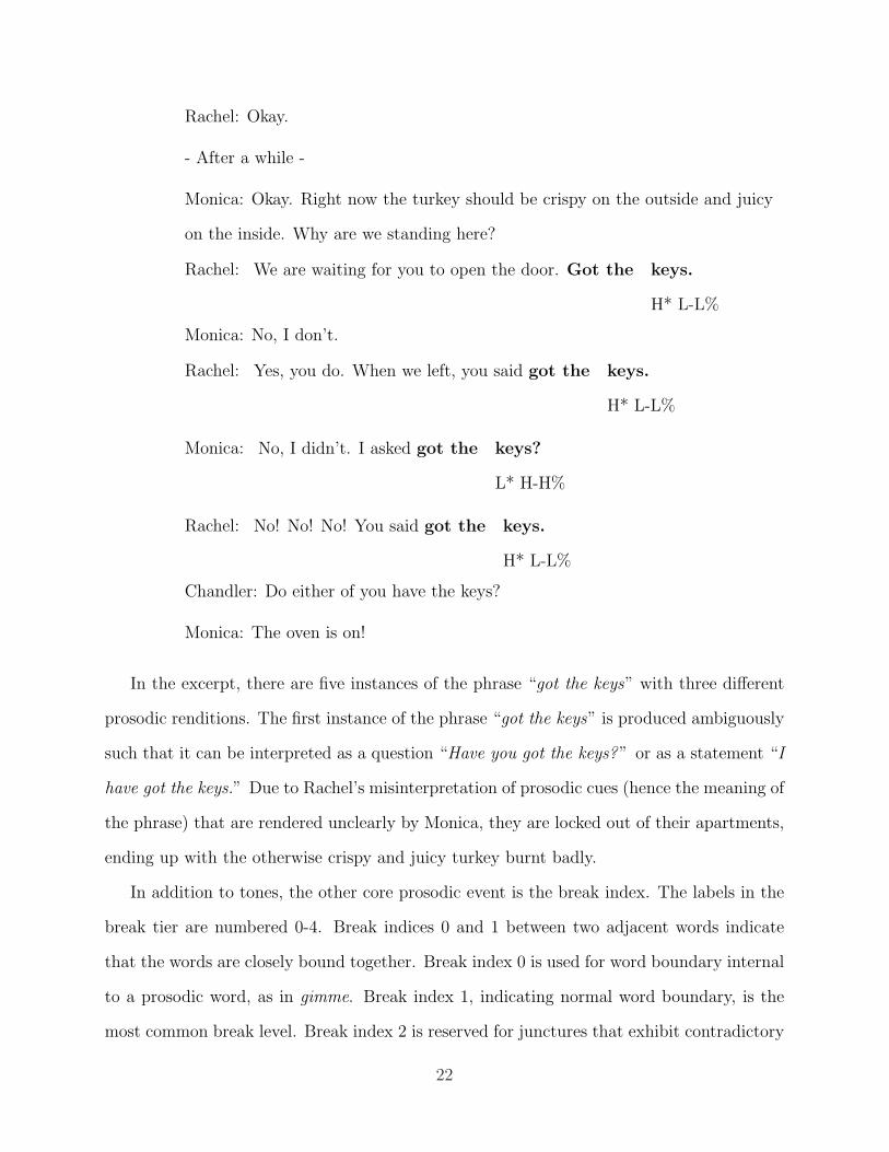
In the excerpt, there are five instances of the phrase “got the keys” with three different

prosodic renditions. The first instance of the phrase “got the keys” is produced ambiguously

such that it can be interpreted as a question “Have you got the keys?” or as a statement “I

have got the keys.” Due to Rachel’s misinterpretation of prosodic cues (hence the meaning of

the phrase) that are rendered unclearly by Monica, they are locked out of their apartments,

ending up with the otherwise crispy and juicy turkey burnt badly.

In addition to tones, the other core prosodic event is the break index. The labels in the

break tier are numbered 0-4. Break indices 0 and 1 between two adjacent words indicate

that the words are closely bound together. Break index 0 is used for word boundary internal

to a prosodic word, as in gimme. Break index 1, indicating normal word boundary, is the

most common break level. Break index 2 is reserved for junctures that exhibit contradictory

22

form, for example, between the observed tonal pattern and the perceptual juncture cues.

Break index 3 is commonly assigned to junctures that exhibit a relatively weak, but clear

break (i.e., intermediate phrase). Break index 4 signals the strongest phrasal level break

(i.e., intonational phrase). A distinction is made between break index 3 (or intermediate

phrase) and break index 4 (or intonational phrase), while all the other indices (0, 1, 2) are

classified as the non-phrasal break category.

Even though the ToBI system posits two different tiers for tonal information and junctural

information, I do not use labels in the break index tier because of the very close association

between the break index 3 and the intermediate phrase, and between the break index 4 and

the intonational phrase.8 Instead, I rely on the symbolic notation available in the tonal tier,

such that dash sign ‘-’ indicating ‘intermediate phrase’ signals a relatively weak break of

index 3, and the percent sign ‘%’ indicating ‘intonational phrase’ signals a relatively strong

break of index 4.

2.3 A Prosodically Labeled Database

In this section I describe the corpus that I use for the analyses and experiments in this dis-

sertation. The corpus used for this work is drawn from a subset of recorded FM public radio

news broadcasts spoken by five radio announcers (Ostendorf, Price, & Shattuck-Hufnagel

1995). The corpus is called the Boston University Radio Speech corpus and is publicly

available through the Linguistic Data Consortium (LDC).9 Radio speech appears to be a

good style for prosody synthesis research, since the announcers strive to sound natural while

8The very close association is mandated in the ToBI guideline, stated as follows: “These two break indexstrengths [i.e., the break indices 3 and 4, TJY] are equated with the intonational categories of intermediate(intonation) phrase and (full) intonation phrase. Thus, whenever the tonal analysis indicates a L- or H-phrase accent, the transcriber should decide where the end of the intermediate phrase marked by this tonelabel is and place a 3 on the break index tier to align with the orthographic label for the last word inthe intermediate phrase. Similarly, whenever the tonal analysis indicates a L% or H% boundary tone,the transcriber should place a 4 on the break index tier at the end of the last word in the intonationphrase.(Beckman & Ayers 1997: 33)”

9http://www.ldc.upenn.edu/

23

reading with communicative intent. The speech style is said to belong to a “natural but

controlled style” (Chen 2004). The work reported in the dissertation is based on the lab-

news portion of the corpus that consists of the recorded speech from 3 female and 2 male

radio announcers.10 Each announcer read the same scripts of four news stories. Thus, each

announcer read about 114 sentences whose average number of words is 16. The four news

scripts were collected in studio recordings, and were later recorded in the laboratory by

multiple announcers. The stories represent independent data, covering different topics and

a different time period.

There are a number of advantages in using the Boston University Radio Speech corpus.

First, probabilistic approaches to the prosodic structure require a large number of instances

in order to estimate parameters properly. The Boston University Radio Speech corpus is

the richest data set that has prosody annotations. Second, it is one of the most widely used

corpora for studies of prosodic structure prediction, whose goal is predicting either prosodic

prominence such as pitch accents or prosodic phrasing such as intonational phrase boundary.

It is, therefore, possible to compare the current results with previously published results.

Finally, because multiple speakers produce the same scripts, it is possible to measure how

similarly or differently a number of different speakers produce prosody.

2.3.1 Frequency

The recent advancement of methodologies for studying the role of frequency and probability

in determining language patterns has fueled discussion on the nature of linguistic rules or

constraints.11 I adopt a probabilistic approach to the analysis of prosodic structure below,

following presentation of raw statistics for pitch accents and boundary tones observed in the

10Note that the corpus is said to have seven speakers, but the portion of the corpus I have used containsonly 5 speakers (3 female and 2 male), and the prosodic labels for one female speaker are only partiallyavailable. Also note that while examining the data set, I sporadically found and hand-corrected regions ofmisalignment.

11See, for example, Bod, Hay, & Jannedy (2003) for the role of probability in a range of subfields oflinguistics including phonology, morphology, syntax, and semantics.

24

Table 2.3: Distribution of pitch accents in the radio speech corpus (The proportion of eachaccent type is in parentheses)

Accents Number of tokens Pitch accents Number of tokensH* 2589 (46.89%) L+H* 1128 (20.43%)!H* 712 (12.89%) *? 291 (5.27%)H+!H* 266 (4.81%) L+!H* 245 (4.43%)L* 228 (4.12%) X*? 31 (0.56%)L*+H 30 (0.54%)

Table 2.4: Distribution of phrasal tones (i.e., intermediate and intonational phrase) in theradio speech corpus (The proportion of each phrasal tone type is in parentheses)

Phrasal tones Number of tokens Phrasal tones Number of tokensL-L% 1026 (35.60%) L-H% 709 (24.60%)!H- 368 (12.76%) L- 344 (11.93%)H- 313 (10.86%) H-L% 82 (2.84%)!H-L% 19 (0.65%) H-H% 12 (0.41%)-?, %?, -X? 9 (0.31%)

radio speech corpus.

The frequency of pitch accents and boundary tones observed in the labnews portion

of the Boston University Radio Speech corpus are presented in Table 2.3 and Table 2.4,

respectively.

There have been arguments for and against the use of frequency or probability in describ-

ing and explaining linguistic systems. Some linguists hold the position that “[O]ne’s ability

to produce and recognize grammatical utterances is not based on notions of statistical ap-

proximation and the like (Chomsky 1957: 16),” whereas others maintain that “[S]tatistical

considerations are essential to an understanding of the operation and development of lan-

guages (Lyons 1968: 98).” In this dissertation, I demonstrate that the analysis of frequency

proves to be useful in evaluating the proposed theory of intonation, but more importantly, it

can be employed in stochastic modeling of prosodic structure. Probabilistic approaches are

better suited to prosodic structure modeling than algorithmic and deterministic approaches.

25

Jackendoff (2002) makes this point clear by stating that “the right approach to these corre-

spondences [between phonology and syntax, TJY] sees Intonational Phrases as phonological

units that on one hand constrain the domains of syllabification, stress, and intonation, and

that on the other bear a loose relation to syntax (p. 119)” and then he stipulates the fol-

lowing formulation rules in (2.3) for rules of intontional phrasing (where IntP stands for

intonational phrase) (Jackendoff 2002: 119).

(2.3) (a) An utterance consists of a series of one or more concatenated IntP’s forming a

flat structure. Each IntP is a sequence of Words.

(b) Preferably, the IntPs are of equal length.

(c) Preferably, the longest IntP is at the end

(d) (Possibly, some strong preferences on maximum duration of IntPs, e.g., try not

to go over three seconds.)

If we agree with Jackendoff (2002) in using terms such as ‘preferably ’ and ‘possibly ’ in de-

scribing the mapping between prosodic structure and other grammatical structures, then we

are led to the conclusion that prosody is better formalized through probabilistic or stochastic

approaches than through deterministic or algorithmic approaches. Stochastic approaches are

data-driven or, in other words, corpus-based. A corpus-based approach can be successfully

implemented only when two requirements are met: one is the availability of corpora, and

the other is the availability of methods that enable one to model prosodic structure on the

corpora. The data are described in this chapter. The data-driven methodologies of prosodic

modeling are described in more detail in Chapter 3.

2.3.2 Reliability of the prosodic labels

The ToBI annotation system is, in essence, a perceptual labeling system. A trained tran-

scriber decides prosodic labels perceptually and manually with the aids of audio-visual

26

display of speech sounds. A number of concerns about the quality of labeling have been

expressed for perceptual/manual labeling in general (Gut & Bayerl 2004), and for ToBI

labeling in particular. Some criticisms concerning the quality of such perceptual/manual

labeling are: First, the manual annotation procedure may be incoherent due to variability in

labelers’ perceptual capabilities and other cognitive factors such as fatigue, motivation and

interest. Second, manual labeling may reflect the variability of the subjective interpretation

and application of the labeling schema by the annotators. And finally, the quality of manual

annotation may be influenced by individual characteristics of the annotator such as his or

her familiarity with the material and the amount of time spent for the training (Gut &

Bayerl 2004).

Some ToBI categories are also called into question by the transcriber reliability studies

as well as recent work in phonetics and psycholinguistics. For example, H* and L+H* are

often confused by trained ToBI labelers (Syrdal & McGory 2000; Herman & McGrory 2002),

and speakers do not distinguish these two categories in production tasks (Dilley 2005; Ladd

& Schepman 2003). For example, Ladd & Schepman (2003) argue that not only L+H*

but also H* has distinct L and H targets. It should be noted, however, that these studies

demonstrate the difficulty of distinguishing the prosodic categories, rather than deny the

existence of these categories.12

To assess the quality of the manual transcription of speech data, various methods have

been proposed and used, including pairwise comparisons between transcribers and Cohen’s

kappa coefficients (Pitrelli, Beckman, & Hirschberg 1994; Syrdal & McGory 2000; Yoon,

Chavarrıa, Cole, & Hasegawa-Johnson 2004, among others).

Two reliability studies have been conducted for the Boston University Radio Speech cor-

pus: One by Ostendorf, Price, and Shattuck-Hufnagel (1995) and the other by Dilley, Breen,

Gibson, Bolivar, and Kraemer (2006). Ostendorf et al.(1995) report that the transcriber

12Depending on one’s necessity and simplification, one may transcribe both L+H* and L*+H as (L+H)*,where the star * outside the parentheses can be linked to either L or H inside the parentheses. Likewiseboth L+H* and H* can be transcribed as (L+)H*.

27

Table 2.5: The amount of speech used for transcriber agreement study by Dilley, Breen,Gibson, Bolivar, & Kraemer (2006)

System Minutes Syllables Coders/File

BURSC 20.9 5939 3.4CallHome 15.2 3680 3.5

agreement in the Boston University Radio Speech corpus is relatively high. Transcribers

agree on the presence or absence of a pitch accent on a particular word in the test sample

91% of the time, and on the type of pitch accent 60% of the time. Disagreement about

pitch accent type is mostly concerned with the choice between H* and L+H* (and !H* and

L+!H*). When these two accent types are combined into one category the level of transcriber

agreement for accent type rises to 81%. The agreement between transcribers regarding the

type of phrasal tone is even higher. When labelers agree that a phrasal tone was present

they agreed on the type of the phrasal tone 91% of the time.

Dilley et al. (2006) also report on transcriber reliability conducted on a subset of the

Boston University Radio Speech corpus, together with a subset of the CallHome corpus.

The CallHome corpus is a corpus of spontaneous nonprofessional speech. Table 2.5 shows

the amount of the data used for the reliability study. Here, the amount of the data in the

Boston University Radio Speech corpus (BURSC) is about one fifth of the amount that I

have used for my experiments in this dissertation.

In Dilley et tal. (2006), the transcribers are five naıve undergraduate students who have

no previous prosodic annotation experience or phonetic training. The naıve transcribers

are trained for ToBI labeling and then annotate about 20 minutes of read speech and 15

minutes of spontaneous speech. The naıve transcribers spent two weeks in being trained in

the ToBI labeling system, and the subsequent four weeks in labeling the speech data. The

transcriber reliability results obtained from that study are as follows: the agreement rate

for the presence of a pitch accent is about 87%, and the rate for the type of pitch accent is

28

about 80%. As for the presence of a phrasal boundary, an agreement rate of 88% is achieved.

An agreement rate for types of phrasal boundary is 76%.13

2.3.3 Speaker consistency of prosodic realization

Little is known about the degree of consistency (or in its opposite sense, variation) in the

realization of prosodic structure. The Boston University Radio Speech corpus consists of

data from five speakers (3 female and 2 male), each reading the same scripts that comprise

more than 110 different sentences. The design of the corpus, thus, proves to be a useful basis

on which we can measure the degree of speaker variation or speaker consistency in prosodic

realization. Below I illustrate how consistent speakers are in rendering prosodic structure

when they speak the same utterance, and then I present the results from my study of the

degree of speaker consistency.

Probably, there would not be a single instance in which two speakers realize exactly the

same prosodic structure phonetically. But the phonetic realization of the intended prosodic

structure is not random either.

Figure 2.4 illustrates the F0 contours of the phrase “Massachusetts may now . . . ” pro-

duced by 5 different speakers (3 female and 2 male) in the radio speech corpus. The corre-

sponding ToBI labels (transcribed by other researchers) are in Table 2.6.14

Figure 2.5 illustrates the F0 contours of the phrases “. . . of the Massachusetts Bar As-

sociation . . . ” produced by 4 different speakers (2 female and 2 male) in the radio speech

corpus, with the corresponding ToBI labels in Table 2.7.15

From Figure 2.4 and 2.5, we observe that some of the characteristics in the F0 contours

13There must be differences in the agreement rates between the read speech style of the Boston UniversityRadio Speech corpus and the spontaneous speech style of the CallHome corpus. No information on thestylistic differences, however, is available regarding the transcriber reliability.

14There must be multiple files that are prosodically labeled by each transcriber, given the reliability studypreviously conducted on this corpus. But the released corpus contains only consensus ToBI labels thattranscribers agreed upon. I used the consensus labels for my experiments in this dissertation.

15As mentioned, some portion of the corpus is not prosodically labeled. So, it is not always possible toillustrate examples by using the same number of speakers.

29

“Massachusetts may now...”

Time (s)0 1.40219

Pitc

h (H

z)

0

450Female 1Female 2Female 3Male 2Male 3

0

75

150

225

300

375

450

Figure 2.4: Overlapped F0 contours of the phrase “Massachusetts may now . . . ” renderedby 3 female and 2 male speakers. The vertical dotted lines indicate the word boundaries(i.e., “Massachusetts | may | now”).

Table 2.6: ToBI labeling of the phrase ‘Massachusetts may now . . . ’

Massachusetts may nowFemale 1 H* !H* L- L+H*Female 2 H* !H* L-L% L*+HFemale 3 H* L+!H* !H- H*Male 2 H* !H* L- H*Male 3 H* !H* !H- H*

Table 2.7: ToBI labeling of the phrase ‘. . . of the Massachusetts Bar Association . . . ’

of the Massachusetts Bar AssociationFemale 1 H* L-H%Female 2 H* L* L-H%Male 2 L+H* H* L-H%Male 3 L+!H* L+H* L-H%

30

“of the Massachusetts Bar Association”

Time (s)0 1.80513

Pitc

h (H

z)

0

350Female 1Female 2Male 2Male 3

0

50

100

150

200

250

300

350

Figure 2.5: Overlapped F0 contours of the phrase “. . . of the Massachusetts Bar Association. . . ” rendered by 4 different speakers (2 female and 2 male). The vertical dotted linesindicate boundaries between two adjacent words.

are shared by all the speakers producing each of the phrases “Massachusetts may now . . . ”

and “. . . of the Massachusetts Bar Association. . . ” For example, all the speakers produce

the highest F0 peak on the first syllable ‘Ma’ in the word ‘Massachusetts ’ in the first phrase,

and on ‘bar ’ in the second phrase.16 From Table 2.6 and Table 2.7, we observe a fair degree

of consistency in the ToBI labeling with respect to the presence or absence of pitch accents

and phrasal tones on the words in each phrase. For example, the word ‘Massachusetts ’ in

the first phrase “Massachusetts may now . . . ” is produced with pitch accents followed by a

tone marking either an intermediate or intonational phrase by all the speakers. Likewise, the

word ‘Bar ’ in the second phrase “. . . of the Massachusetts Bar Association. . . ” is produced

with a pitch accent by all speakers and the transcribers assigned either H* or L+H* to the

16Incidentally, the highest F0 peak is observed to occur at the secondary, not primary, stressed syllable inthe word “Massachusetts” of the 1st phrase.

31

word ‘Bar.’

Despite similarity in the F0 contours produced by multiple speakers and higher rate

of consistency in transcribed prosodic labels, there is some discrepancy between tune and

prosodic transcription. For example, similar shapes can lead to different transcriptions and

different shapes lead to the same transcription. Specifically, in Figure 2.5, the F0 contours

of the word “bar” produced by Male 3 and produced by Female 1 look more similar to each

other than the F0 contours produced by other speakers. But, one is transcribed with a rising

“L+H*” accent, and the other is transcribed with a plain “H*” accent. The example may be a

case where the F0 contour is not in a perfect mapping relationship with a perceptual prosodic

event. There are two sources of a mismatch between an F0 contour and the corresponding

labeled tonal event. One is inconsistency in prosodic labeling, for which the above-mentioned

studies on transcriber reliability are useful. The other is that F0 contours are only one of

the properties that determine perceptual prosodic events. It should be noted that while the

ToBI label is influenced by the visual display of F0 contours, the system is not a phonetic

transcription system, but a phonological model of intonation. The phonetic F0 shape and

its perceived prosodic event may or may not be in a perfect mapping relation. As to the

question of how much the F0 shape contributes to the prosodic label, prosodic modeling

using features obtained from those F0 shapes would prove to be useful, which is addressed

in Chapter 5.

Next, I address the question of how consistently different speakers render prosodic struc-

ture when they are telling the same stories. In Yuan, Brenier, & Jurafsky (2005), inter-

speaker variation is investigated regarding the presence or absence of pitch accent. The

aim of their study is to test whether inter-speaker variability has any effect on the task of

predicting the presence or absence of pitch accent. The prosodic information of one speaker

is trained and the trained model is applied to other speakers. Based on the consistent rate

of accuracy across speakers, they conclude that interspeaker variability does not markedly

influence prosodic prominence prediction. My study reported here replicates this earlier

32

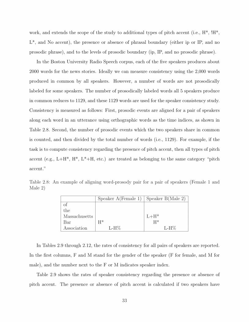
work, and extends the scope of the study to additional types of pitch accent (i.e., H*, !H*,

L*, and No accent), the presence or absence of phrasal boundary (either ip or IP, and no

prosodic phrase), and to the levels of prosodic boundary (ip, IP, and no prosodic phrase).

In the Boston University Radio Speech corpus, each of the five speakers produces about

2000 words for the news stories. Ideally we can measure consistency using the 2,000 words

produced in common by all speakers. However, a number of words are not prosodically

labeled for some speakers. The number of prosodically labeled words all 5 speakers produce

in common reduces to 1129, and these 1129 words are used for the speaker consistency study.

Consistency is measured as follows: First, prosodic events are aligned for a pair of speakers

along each word in an utterance using orthographic words as the time indices, as shown in

Table 2.8. Second, the number of prosodic events which the two speakers share in common

is counted, and then divided by the total number of words (i.e., 1129). For example, if the

task is to compute consistency regarding the presence of pitch accent, then all types of pitch

accent (e.g., L+H*, H*, L*+H, etc.) are treated as belonging to the same category “pitch

accent.”

Table 2.8: An example of aligning word-prosody pair for a pair of speakers (Female 1 andMale 2)

Speaker A(Female 1) Speaker B(Male 2)oftheMassachusetts L+H*Bar H* H*Association L-H% L-H%

In Tables 2.9 through 2.12, the rates of consistency for all pairs of speakers are reported.

In the first columns, F and M stand for the gender of the speaker (F for female, and M for

male), and the number next to the F or M indicates speaker index.

Table 2.9 shows the rates of speaker consistency regarding the presence or absence of

pitch accent. The presence or absence of pitch accent is calculated if two speakers have

33

any type of pitch accent on the aligned words. On average, the rate of consistency on the

presence or absence of pitch accent is 79.81%.17

Table 2.9: Rate of consistency on the presence or absence of pitch accent for each pair ofspeakers. Average consistency rate is 79.81%

Speaker Speaker Ratio ConsistencyF1 F2 912/1129 80.77%F1 F3 878/1129 77.76%F1 M2 886/1129 78.47%F1 M3 897/1129 79.45%F2 F3 899/1129 79.62%F2 M2 911/1129 80.69%F2 M3 904/1129 80.07%F2 M2 901/1129 79.80%F3 M3 906/1129 80.24%M2 M3 918/1129 81.31%

Average 79.81%

In Table 2.10, the results of the presence or absence of boundary tone are presented for

each pair of speakers. In case of the speaker F1, the ratio and rate of consistency with

speakers F3 and M3 are reported to be the same. On average, a 89.71% consistency rate is

achieved.

In Table 2.11 is presented the pair-wise consistency rate of types of pitch accents. Here,

the types are broadly classified to be H*, !H*, L*, and no pitch accent, on the basis of

the tonal target (i.e., starred tone). Any pitch accents containing H* (i.e., H*, L+H*) and

H+!H*18 are classified to be H*. Any pitch accents containing downstepped !H* except

H+!H* (i.e., !H*, L+!H*) are treated as !H*. Finally, both L* and L*+H are treated as

members of the L* category. If two speakers share in the production of the broad types of

pitch accents, then it is decided that they are consistent in rendering the type of prosodic

prominence. Overall, an average consistency of 72.17% is achieved for the rate of consistency

for the types of the pitch accent.

17The chance rate of consistency for a pair of speakers is 50%.18H+!H* is treated as H*, not as !H*, because H+!H* has high tone target preceded by (or a step down

from) an even higher pitch.

34

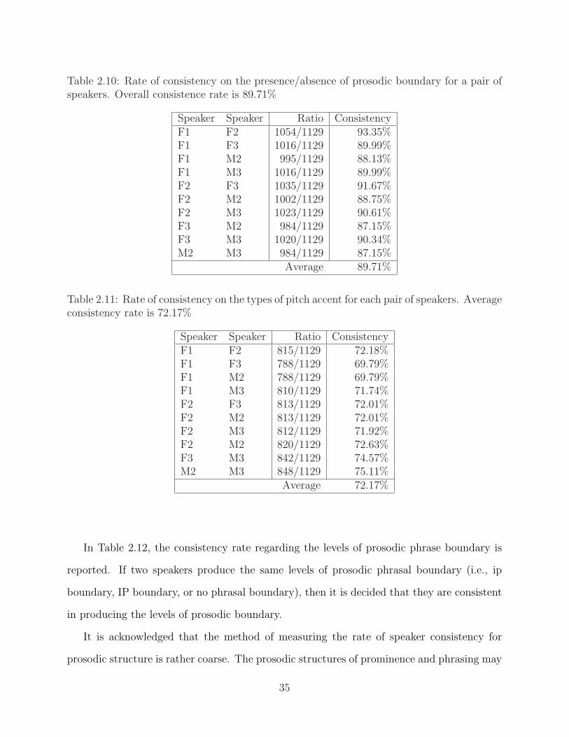
Table 2.10: Rate of consistency on the presence/absence of prosodic boundary for a pair ofspeakers. Overall consistence rate is 89.71%

Speaker Speaker Ratio ConsistencyF1 F2 1054/1129 93.35%F1 F3 1016/1129 89.99%F1 M2 995/1129 88.13%F1 M3 1016/1129 89.99%F2 F3 1035/1129 91.67%F2 M2 1002/1129 88.75%F2 M3 1023/1129 90.61%F3 M2 984/1129 87.15%F3 M3 1020/1129 90.34%M2 M3 984/1129 87.15%

Average 89.71%

Table 2.11: Rate of consistency on the types of pitch accent for each pair of speakers. Averageconsistency rate is 72.17%

Speaker Speaker Ratio ConsistencyF1 F2 815/1129 72.18%F1 F3 788/1129 69.79%F1 M2 788/1129 69.79%F1 M3 810/1129 71.74%F2 F3 813/1129 72.01%F2 M2 813/1129 72.01%F2 M3 812/1129 71.92%F2 M2 820/1129 72.63%F3 M3 842/1129 74.57%M2 M3 848/1129 75.11%

Average 72.17%

In Table 2.12, the consistency rate regarding the levels of prosodic phrase boundary is

reported. If two speakers produce the same levels of prosodic phrasal boundary (i.e., ip

boundary, IP boundary, or no phrasal boundary), then it is decided that they are consistent

in producing the levels of prosodic boundary.

It is acknowledged that the method of measuring the rate of speaker consistency for

prosodic structure is rather coarse. The prosodic structures of prominence and phrasing may

35

Table 2.12: Rate of consistency on the levels of prosodic boundary for a pair of speakers.Average consistence rate is 79.25%

Speaker Speaker Ratio ConsistencyF1 F2 923/1129 81.75%F1 F3 892/1129 79.00%F1 M2 889/1129 78.74%F1 M3 905/1129 80.15%F2 F3 891/1129 78.91%F2 M2 860/1129 76.17%F2 M3 900/1129 79.71%F3 M2 872/1129 77.23%F3 M3 922/1129 81.66%M2 M3 894/1129 79.18%

Average 79.25%

be influenced by each other, such that a pitch accent on a given word may be influenced by

the presence of a boundary nearby (i.e., rhythmic factors), in addition to or instead of being

influenced by the information status such as topic or focus of the word (cf. Selkirk 1984).

Nevertheless, the study of inter-speaker consistency as reported here provides us with some

revealing insights: First, the high rates of consistency for the presence or absence of pitch

accent and of boundary tone indicates that despite the observed inter-speaker variation, there

must be constraints imposed on prosodic structure, and the constraints must be stronger in

the determination of prosodic phrasing than prosodic prominence. If prosodic phrasing were

isomorphic with syntactic phrasing, the consistency would be 100%. A speculation is that the

syntactic phrasing, though not isomorphic, plays a significant role in determining the location

of prosodic phrase boundaries. Nevertheless, other factors such as transcribers expectations

about prosodic structure and their sensitivity to different speakers may contribute to the

observed variability. It is also the case that effectiveness in encoding prosodic structure is

different among different speakers. Informally, I observed that the male speaker M3 speaks

some parts of the scripts rather in a slurring manner and that the ToBI transcription of

36

those intervals contains uncertainty or ambiguous labels.

Second, the relatively low rate of 79.25% for the consistency of choosing the level of

prosodic boundary of intermediate or intonational phrase, compared to the rate of 89.71%

for the consistency of choosing the presence or absence of prosodic boundary, may be an

indirect indicator that there is more freedom of choice for a given speaker in choosing either

level of prosodic phrase boundary than there is for the presence or absence of a boundary, or

that transcribers are not good at hearing the distinctions in phrase boundary level compared

to the prosodic boundary.

2.4 Conclusion

In this chapter the ToBI system is described, with special emphasis on the tonal categories

for prosodic prominence and boundary. The Boston University Radio Speech corpus is then

presented, which is one of the largest prosodically-labeled corpora. The corpus contains

prosodic labels based on the ToBI annotation system. I concluded the chapter by reviewing

the earlier studies of transcriber reliability conducted on this corpus, and by presenting the

rate of speaker consistency in rendering prosodic events of an utterance by five different

speakers.

The discussion in this chapter is motivated by the following points: Formalization of

prosodic structure is better expressed through probabilistic or stochastic approaches than

through deterministic, algorithmic approaches. The stochastic approach, however, is data-

driven or corpus-based, which requires two components: one is the availability of data and

the other is the availability of methods and tools. In this chapter, I presented one database

with prosodic labels, together with an analysis of the inter-transcriber reliability and the

rate of speaker consistency. Methodologies that can be used for the stochastic modeling of

prosodic structure are to be discussed in the next chapter.

37

Chapter 3

Machine Learning and itsApplications to Prosody Modeling

3.1 Introduction

Probabilistic approaches are more suitable than deterministic approaches in describing and

modeling prosodic structure. Stochastic approaches require large scale corpora for proper

parameter estimation. The Boston University Radio Speech corpus with manually anno-

tated prosodic labels is one such corpus that meets the requirement. In addition to the

database, the proper methodologies and techniques are required to analyze or design models

of prosodic structure. Machine learning algorithms are one of the methodologies that meet

this additional requirement.

Machine learning algorithms aim to find generalizations over data. The most attractive

characteristic of machine learning algorithms is that the mapping functions trained and

obtained from speech data can be used, for example, to obtain prosodic labels such as pitch

accents and boundary tones from new speech data of a similar style. In this chapter, I

introduce two machine learning algorithms: memory-based learning (MBL) algorithm, and

classification and regression tree (CART). The description of the algorithms is followed by

standard evaluation metrics such as baseline, accuracy, precision, recall, and F-score, that are

typically employed to evaluate the performance of machine learning algorithms. Finally, the

chapter concludes with the review of earlier studies on the prediction of prosodic structure.

38

3.2 Machine Learning

Machine learning has developed out of the research field of Artificial Intelligence, and has a

strong relation with statistics and probability. It is gaining popularity in many aspects of

natural language processing including learning of phonotactics, morphological learning, part

of speech (POS) tagging, syntactic and semantic parsing, and machine translation. Machine

learning algorithms can be divided into two main categories: supervised and unsupervised

machine learning algorithms. In supervised learning, the input of the learning algorithm

consists of examples (in the form of feature vectors) with a class label assigned to them.

Supervised learning algorithms aim to learn to assign correct labels to new unseen examples

of the same task. Unsupervised algorithms learn from unlabeled examples. Unsupervised

learning may aim to cluster examples on the basis of their similarity. In this dissertation, I

focus on supervised learning algorithms, and throughout the discussion, I will use the term

“learning algorithms” to refer to supervised learning algorithms.

A machine learning algorithm in general consists of three components: (1) a learning

component, (2) a model, and (3) a classification component (Hendrickx 2005). The learning

component seeks to find an optimal mapping function on the basis of labeled examples. The

labeled examples are referred to as instances, observations, or tokens in the literature, and

I use these terms interchangeably. Formally, the set of labeled training instances forms the

basis on which some competing functions (also called hypotheses) f : X → Y that map an

instance x ∈ X to a class y ∈ Y are evaluated. For example, features that characterize

the element x of X may consist of part of speech tags (e.g., {Noun, Verb, Noun, Verb,

Determiner, . . .}) , and Y may be a set composed of the elements {pitch accent, No pitch

accent}. The algorithm induces a hypothesis f ′ of the target function f on the basis of a set

of labeled training instances. This induced hypothesis is stored in the form of some model

of the target function. The true target function f is not directly available to the learner; It

is only implicitly estimated through the class labels assigned to the set of instances. The

39

classification component takes unseen instances as input and applies the stored model to

predict class labels for the unseen instances. An instance are represented as a set of features.

Features is the properties that describe an instance as the characteristic of that instance that

are available as input to the classification function. Thus, two important factors in machine

learning algorithms are 1) the input features to use, and 2) algorithms to evaluate the input

features.

There exist many machine algorithms, depending on the way a hypothesis f ′ is searched.

“Inducing a hypothesis f ′ of the true target function f is viewed as a search in a hypothesis

space that represents all possible hypotheses (Hendrickx 2005: 3).” This hypothesis space is

defined by the hypothesis representation chosen by particular machine learning algorithms

(Mitchell 1997; Hendrickx 2005; Bishop 1995). Some of the widely known machine learning

algorithms include Decision Tree or classification and regression tree (CART), memory-based

learning (MBL), Artificial Neural Network (ANN), Support Vector Machine (SVM), Sparse

Network of Winnow (SNoW), Maximum Entropy (MaxEnt), Conditional Random Field

(CRF), and Hidden Markov Model (HMM).

In what follows, I describe two machine learning algorithms, the memory based learning

(MBL) algorithm as implemented in TiMBL (Daelemans et al. 2004), and the classifica-

tion and regression tree (CART) algorithm. Implemented variants of CART include C4.5

(Quinlan 1986) and Wagon (Taylor, Caley, Black, & King 1999), among others. These two

algorithms are chosen due to their flexibility and efficiency in dealing with both continuous

and categorical variables.1 Especially, most earlier studies on the prosodic prediction task

use a variant of CART as a learning algorithm, which makes is necessary to understand how

the algorithm works.

1It should be noted that not every algorithm can deal with both continuous and categorical variables,without manipulating data representation.

40

3.2.1 Memory-based learning (MBL)

The description of the memory-based learning (MBL) algorithm described below is based

on Daelemans et al. (2004). The fundamental assumption of MBL is that “performance in

cognitive tasks is based on reasoning on the basis of similarity of new situations to stored rep-

resentations of earlier experiences, rather than on the application of mental rules abstracted

from earlier experiences (as in rule induction and rule-based processing)” (Daelemans et

al. 2004:18-19). The MBL system, as is the case with other machine learning algorithms,

contains two components: (1) a learning component, and (2) a performance component.

The learning component of MBL is memory-based as it involves adding training instances

to memory. MBL is sometimes referred to as ‘lazy learning’ or ‘exemplar learning’ as memory

storage is done without abstraction or restructuring. The performance component deals with

the product of the learning component. The product is a model serving as a basis for mapping

input to output. The performance takes the form of classification. During classification, a

previously unseen test instance is presented to the system. The similarity between the new

instance X and all examples Y in memory is computed using some distance metric ∆(X,Y ).

Extrapolation is done by assigning the most frequent category within the found set of most

similar examples (i.e., the k-nearest neighbors) as the category of the new test instance.

The k-nearest neighbor (or k-nn) is an algorithm, according to which a new instance is

classified based on the majority of category among the k-nearest neighbor training instances.

The k-nn algorithm is related to nonparametric density estimation. Non-parametric function

is used when probability density function is not specified in advance, but depends on the

data itself. The non-parametric probability density function estimation is generally expressed

as P (x) ∼= KNV

, where K is the number of instances inside the volume V , V is the volume

surrounding x, and N is the total number of instances (Bishop 1995). The density estimation

is usually computed by either of the following two ways: One way is fixing the volume V and

determining the number of K of data points inside the volume V , and this is an approach

41

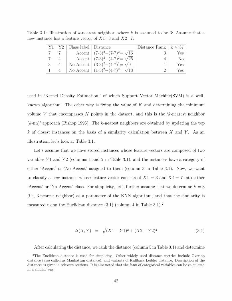
Table 3.1: Illustration of k-nearest neighbor, where k is assumed to be 3: Assume that anew instance has a feature vector of X1=3 and X2=7.

Y1 Y2 Class label Distance Distance Rank k ≤ 3?

7 7 Accent (7-3)2+(7-7)2=√

16 3 Yes

7 4 Accent (7-3)2+(4-7)2=√

25 4 No

3 4 No Accent (3-3)2+(4-7)2=√

9 1 Yes

1 4 No Accent (1-3)2+(4-7)2=√

13 2 Yes

used in ‘Kernel Density Estimation,’ of which Support Vector Machine(SVM) is a well-

known algorithm. The other way is fixing the value of K and determining the minimum

volume V that encompasses K points in the dataset, and this is the ‘k-nearest neighbor

(k-nn)’ approach (Bishop 1995). The k-nearest neighbors are obtained by updating the top

k of closest instances on the basis of a similarity calculation between X and Y . As an

illustration, let’s look at Table 3.1.

Let’s assume that we have stored instances whose feature vectors are composed of two

variables Y 1 and Y 2 (columns 1 and 2 in Table 3.1), and the instances have a category of

either ‘Accent’ or ‘No Accent’ assigned to them (column 3 in Table 3.1). Now, we want

to classify a new instance whose feature vector consists of X1 = 3 and X2 = 7 into either

‘Accent’ or ‘No Accent’ class. For simplicity, let’s further assume that we determine k = 3

(i.e, 3-nearest neighbor) as a parameter of the KNN algorithm, and that the similarity is

measured using the Euclidean distance (3.1) (column 4 in Table 3.1).2

∆(X, Y ) =√

(X1− Y 1)2 + (X2− Y 2)2 (3.1)

After calculating the distance, we rank the distance (column 5 in Table 3.1) and determine

2The Euclidean distance is used for simplicity. Other widely used distance metrics include Overlapdistance (also called as Manhattan distance), and variants of Kullback Leibler distance. Description of thedistances is given in relevant sections. It is also noted that the k-nn of categorical variables can be calculatedin a similar way.

42

nearest neighbors based on k-th minimum distance. Under the condition of k = 3, we have

2 ‘No Accent’ instances and 1 ‘Accent’ instance (the last column in Table 3.1). Using the

criterion of majority voting, we conclude that a new instance with feature values X1 = 3

and X2 = 7 is classified in the ‘No Accent’ category. In this dissertation, k = 1, a default

parameter value, is used, unless specified otherwise.

The distance metric ∆(X, Y ) utilized in the TiMBL algorithm is an overlap metric (Daele-

mans et al. 2003). An overlap metric is also called Hamming distance, Manhattan distance,

city-block distance, or L1 distance. The overlap metric is given in (3.2) through (3.4), where

∆(X, Y ) is the distance between instances X and Y . Both X and Y are represented by n

features, and δ is the distance per features.

∆(X,Y ) =∑

i

δ(xi, yi) (3.2)

where the distance is calculated as in (3.3) if the variable is continuous

δ(xi, yi) = abs(

xi − yi

maxi −mini

)(3.3)

Or, it is calculated as in (3.4) if the variable is categorical

δ(xi, yi) =

0 if xi = yi

1 if xi 6= yi

(3.4)

As can be seen in the distance metric (3.3) and (3.4), the memory-based learning can

learn from both continuous and categorical variables. If the variable is continuous, the range

of the variable is controlled by the values max and min. This indicates that for the optimal

learning of a continuous variable, normalization needs to be done in order to ensure that

different variables are treated with roughly comparable levels of importance by the learning

algorithm. With categorical variables, the distance metric in (3.4) simply counts the number

of mismatching feature-values in both categorical features.

43

A common intuition, especially for tasks with many features, is that some features are

more important than others for classification. Not all the features may be good predictors

of the class labels. So we may want to find out which features are good predictors of the

class labels by computing statistics about the relevance of features. Information Gain (IG)

is one such measure that weights features by measuring how much each feature in isolation

contributes to our knowledge of the correct class label. That is, Information Gain of the

feature i is measured by computing the difference in uncertainty as measured by entropy

between the situation without and with knowledge of the value of that feature, as in (3.5).

wi = H(C)− ∑

v∈Vi

P (v)×H(C|v) (3.5)

where C is the set of class labels, Vi is the set of values for feature i, and H(C) is the entropy

of the class labels. The entropy is calculated using the formula in (3.6). 3

H(C) = −∑

c∈C

P (c) log2 P (c) (3.6)

Information Gain, however, tends to overestimate the relevance of features with large

numbers of values. To normalize Information Gain for features with different numbers of

values, the Gain Ratio which is introduced by Quinlan (1993) is used. The Gain Ratio is

Information Gain divided by si(i), as in (3.7). Here, si(i) is called ‘split info’ and denotes

the entropy of the feature-values, as in (3.8)

wi =H(C)−∑

v∈ViP (v)×H(C|v)

si(i)(3.7)

3Entropy has a value from 0 to 1, with 0 being the most certain and 1 the most uncertain. For example,let’s assume that the probability of content words to be accented is 95%, and the probability of functionwords to be accented is 10%. We can express the probability distribution as P = (0.95, 0.10), and calculatethe information conveyed by the entropy as in H(P ) = −(0.95· log2(0.95) + 0.1· log2(0.1)) = 0.4, where 2 isused as the base of the logarithm.

44

si(i) = − ∑

v∈Vi

P (v) log2 P (v) (3.8)

The resulting Gain Ratio values is then used as weights wi in the weighted distance

metric, as in (3.9).

∆(X,Y ) =∑

i

wiδ(xi, yi) (3.9)

The weighted distance metric (3.9) is called “IB1-IG”, and is used in the experiment

reported in the next chapter.4

3.2.2 Classification and regression tree (CART)

A decision tree classifier refers to a set of machine learning algorithms that derive abstract

rules from the training instances, and then use these rules when predicting the class labels of

test instances. Two best of the known variants of the decision tree algorithm are classification

and regression tree (CART) (Breiman et al. (1984)), and C4.5 (Quinlan (1986, 1993)). The

two algorithms are similar to each other. First, both involve “partitioning the input space

into regions and fitting a different mapping within each region (Bishop 1995).” Second,

the two algorithms can use both rules induced by statistical learning and rules constructed

by expert knowledge in order to build binary decision trees. The binary decision trees are

formulated as a set of ordered yes-no questions about the features in the data.

The advantages of the tree-based decision algorithm over other machine learning models

include manual construction of rules, robustness to outliers and mislabeled data samples, and

data samples with some missing features, and efficient prediction of instances that consist of

both categorical and continuous features (Huang, Acero, & Hon 2001). Due to its simplicity

and robustness, many software packages implement variants of a decision tree, including

4In addition to the default parameters, other methods of distance metrics, feature weighting, and distanceweighting are also implemented in TiMBL. I will address some of the alternatives in Chapter 5. Possibleparameters that can be used in TiMBL are described in Daelemans et al. (2004).

45

“wagon” in the Edinburgh Speech Tools Library (Taylor et al. 1999) and AT&T CART

(Riley 1992), among others.

CART is, in essence, a greedy algorithm in that a greedy search is conducted to find the

best splitting rule. Initially, all instances are considered to belong to a single group. The

operation of sets of splitting rules, stopping rules, and prediction rules is used to produce a

particular decision tree for a given data set. The group is split into two subgroups using,

say, high values of a variable for one group and low values for the other. The splitting into

leaf nodes is based on the criterion of minimizing prediction error rate. The minimization

of the error rate is estimated by calculating minimum prediction error rates on the training

data (Riley 1992; Wang & Hirschberg 1992). Stopping rules terminate the splitting process

at some node in the tree, resulting in terminal nodes. Prediction rules assign class labels to

the terminal nodes. For continuous variables, the prediction rules calculate the mean of the

data points classified together at that node. For categorical variables, the rules choose the

class that occurs most frequently among the data points.

A CART presentation is exemplified in Figure 3.1.

In Figure 3.1, the CART representation is designed to classify the presence or absence of

an intonational phrase boundary on a word. The tree is made for illustration purpose only.

The features for this graphical display are extracted from the training portion of the radio

speech corpus. Features present in the tree include silent pause following the word (‘sil’ for

a silent pause or ‘no-sil’ for no silent pause), the word duration (‘word-dur’ in msec), the

number of syllables in the word (‘numSyllable’), the index of syntactic phrase in reverse

order (‘SynPhrase id’) , and the intonational phrase based normalized F0 extracted from

5 equally spaced points within the word (e.g., ‘norm-f0 4’ stands for the fourth normalized

F0). The features are described in detail in Chapter 4 and Chapter 5.

In the tree, all instances are considered as a single group ‘word’ initially.5 The group

5In Figure 3.1, the non-terminal grouping of objects in the binary decision tree is indicated by the circle,and the terminal grouping is indicated by the rectangle.

46

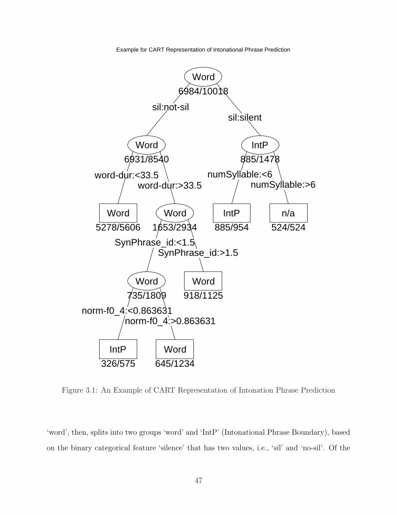
Example for CART Representation of Intonational Phrase Prediction

sil:not-silsil:silent

6984/10018

Word

word-dur:<33.5word-dur:>33.5

6931/8540

Word

5278/5606

Word

SynPhrase_id:<1.5SynPhrase_id:>1.5

1653/2934

Word

norm-f0_4:<0.863631norm-f0_4:>0.863631

735/1809

Word

326/575

IntP

645/1234

Word

918/1125

Word

numSyllable:<6numSyllable:>6

885/1478

IntP

885/954

IntP

524/524

n/a

Figure 3.1: An Example of CART Representation of Intonation Phrase Prediction

‘word’, then, splits into two groups ‘word’ and ‘IntP’ (Intonational Phrase Boundary), based

on the binary categorical feature ‘silence’ that has two values, i.e., ‘sil’ and ‘no-sil’. Of the

47

data, 6984 out of 10018 (or 68.84%) are correctly classified on this binary distinction alone.

The second ‘word’ group on the left splits further on the basis of numerical feature of the

duration of the word. That is, if the word is not followed by any silent pause, and the

duration of that word is less than 33.5ms, then the word is classified as the one followed by

normal word boundary. In this way, we can correctly classify about 84% of the test data

with respect to the presence or absence of an intonational boundary. It should be noted,

however, that the performance of the CART is not optimized, and that only part of the full

tree nodes are shown for a illustration purpose.

In a similar vein, a CART can be constructed that aims to predict the presence or absence

of pitch accent, as in Figure 3.2.

For the task, 848 words out of 1054 words in the test data, that is, 80.45% is correctly

classified as either having pitch accent or not. In the figure, ‘f0-b0’, ‘f0-b1’, ‘f0-b2’, and ‘f0-b3’

denote four F0 related coefficients obtained through third-order polynomial decomposition,

and ‘numPhone’ stands for the number of phones in a word. The features are described in

detail in Chapter 4 and Chapter 5.

C4.5 is another variant of the decision tree algorithm, and it differs from the CART

algorithm in that C4.5 uses a population probability distribution in deciding the splitting of

binary tree. CART as originally proposed by Breiman, Friedman, Olshen, & Stone (1984) is

not tied to any underlying population probability distribution of input features (Johnson &

Wichern 2002). In designing the decision tree algorithm of C4.5, Quinlan (1986, 1993) intro-

duces Entropy and Information Gain (IG) which take the population probability distribution

into consideration.6 The introduction of Entropy and Information Gain into the learning

algorithm is motivated by the observation that features with higher information gain in the

training data are likely to be more useful for a classification task. Entropy, as formulated in

(3.6), is a measure of uncertainty in a set of training instances. Information Gain (IG) of a

feature is the expected reduction in entropy, or the expected reduction in uncertainty, and

6See the formula (3.5)-(3.7) above for Entropy (3.6), Information Gain (3.5), and Gain Ratio (3.7)

48

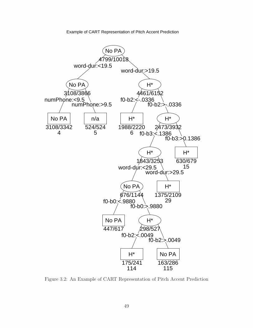
Example of CART Representation of Pitch Accent Prediction

word-dur:<19.5word-dur:>19.5

4799/10018

No PA

numPhone:<9.5numPhone:>9.5

3108/3866

No PA

43108/3342

No PA

5524/524

n/a

f0-b2:<-.0336f0-b2:>-.0336

4461/6152

H*

61988/2220

H*

f0-b3:<.1386f0-b3:>0.1386

2473/3932

H*

word-dur:<29.5word-dur:>29.5

1843/3253

H*

f0-b0:<.9880f0-b0:>.9880

676/1144

No PA

447/617

No PA

f0-b2:<.0049f0-b2:>.0049

298/527

H*

114175/241

H*

115163/286

No PA

291375/2109

H*

15630/679

H*

Figure 3.2: An Example of CART Representation of Pitch Accent Prediction

49

is estimated by considering the uncertainty when the feature is known. Features with higher

Information Gain (IG) are likely to be more useful. Other than the population probability

distribution as measured by Entropy and Information Gain, the C4.5 and CART share many

characteristics in common.

3.3 Evaluation Metric

3.3.1 Baselines

An important concept in machine learning is the baseline. This is the performance of the

simplest classifier one can think of. For part-of-speech tagging, for example, the baseline

is usually taken to be the accuracy achieved when predicting always the most probable tag

of a word. In this sense, the baseline is also called chance level performance. In a similar

vein, for the presence or absence of prosodic phrasing, the baseline is the accuracy achieved

when predicting always the most probable event, i.e., either the percentage of the presence

of prosodic phrasing, or the percentage of the absence of prosodic phrasing over the total

number of words. In predicting the presence or absence of prosodic phrasing, the most

probable class of an instance is “no prosodic phrasing.” Always predicting “no prosodic

phrasing” would always result in an accuracy of 72% on the data set. Thus, performance of

the learning algorithm can be evaluated based on the gain made compared to baseline. If

the baseline is over 94%, a performance of 95% is a mere 1% absolute increase.7

3.3.2 Evaluation Metric

In many machine learning experiments, “best” performance means the one with the best

generalized accuracy on previously unseen test instances, i.e., with the percentage of correctly

7Absolute gain is different from relative gain. If 85% is the best one can achieve using a particularoptimized learning algorithm, then 86%, which is an increase of relative 1%, may be tremendously difficultto achieve.

50

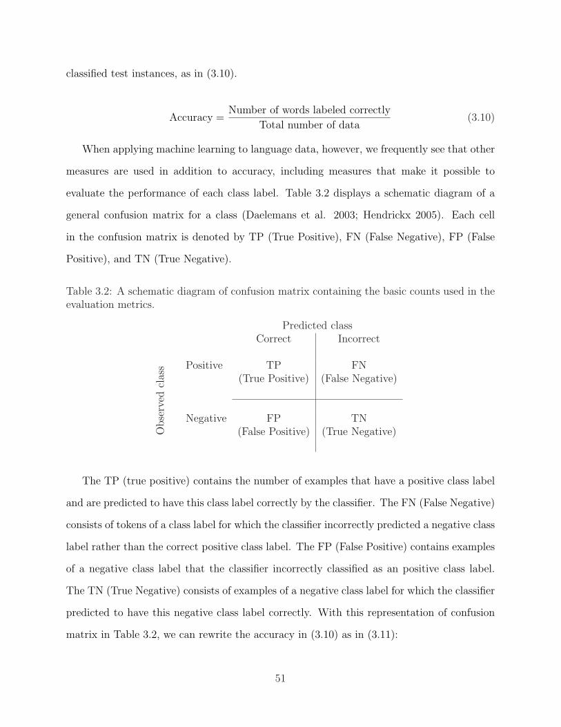
classified test instances, as in (3.10).

Accuracy =Number of words labeled correctly

Total number of data(3.10)

When applying machine learning to language data, however, we frequently see that other

measures are used in addition to accuracy, including measures that make it possible to

evaluate the performance of each class label. Table 3.2 displays a schematic diagram of a

general confusion matrix for a class (Daelemans et al. 2003; Hendrickx 2005). Each cell

in the confusion matrix is denoted by TP (True Positive), FN (False Negative), FP (False

Positive), and TN (True Negative).

Table 3.2: A schematic diagram of confusion matrix containing the basic counts used in theevaluation metrics.

Predicted classCorrect Incorrect

Positive TP FN(True Positive) (False Negative)

Negative FP TN

Obse

rved

clas

s

(False Positive) (True Negative)

The TP (true positive) contains the number of examples that have a positive class label

and are predicted to have this class label correctly by the classifier. The FN (False Negative)

consists of tokens of a class label for which the classifier incorrectly predicted a negative class

label rather than the correct positive class label. The FP (False Positive) contains examples

of a negative class label that the classifier incorrectly classified as an positive class label.

The TN (True Negative) consists of examples of a negative class label for which the classifier

predicted to have this negative class label correctly. With this representation of confusion

matrix in Table 3.2, we can rewrite the accuracy in (3.10) as in (3.11):

51

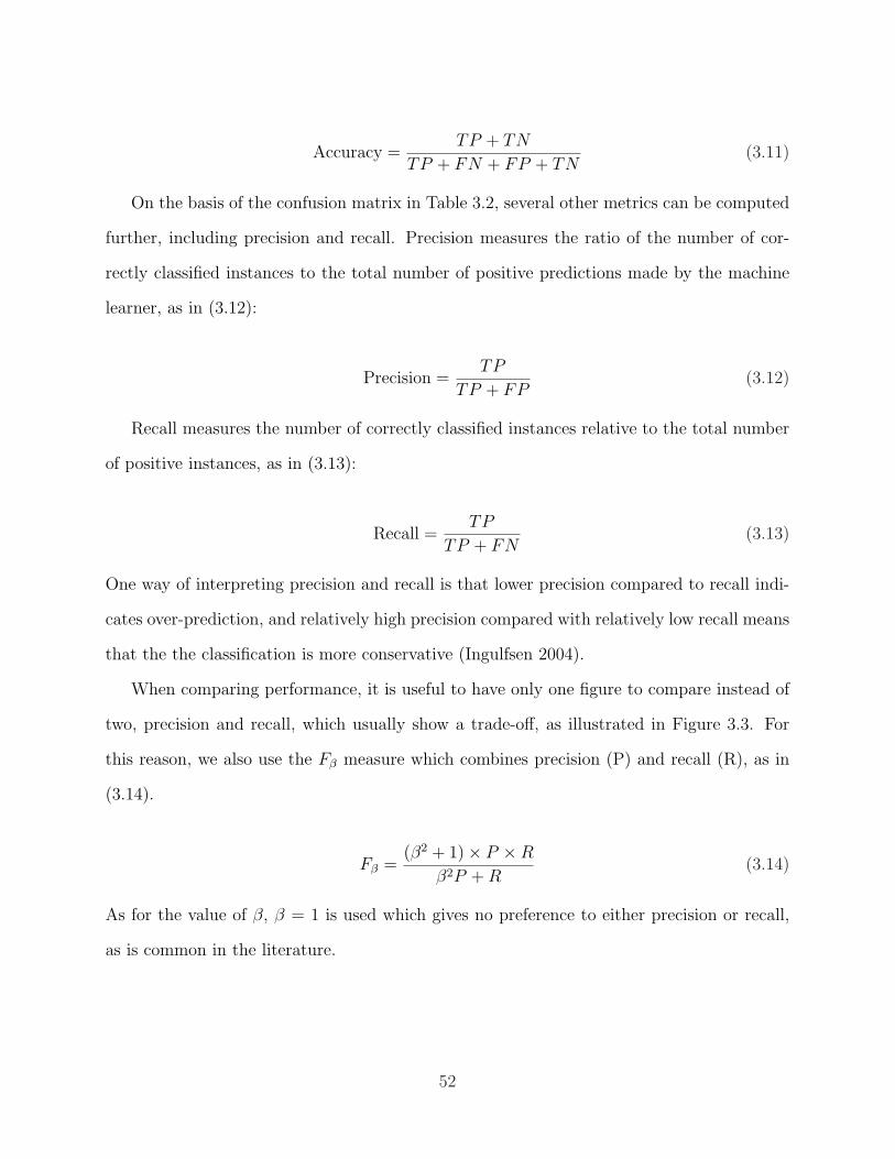
Accuracy =TP + TN

TP + FN + FP + TN(3.11)

On the basis of the confusion matrix in Table 3.2, several other metrics can be computed

further, including precision and recall. Precision measures the ratio of the number of cor-

rectly classified instances to the total number of positive predictions made by the machine

learner, as in (3.12):

Precision =TP

TP + FP(3.12)

Recall measures the number of correctly classified instances relative to the total number

of positive instances, as in (3.13):

Recall =TP

TP + FN(3.13)

One way of interpreting precision and recall is that lower precision compared to recall indi-

cates over-prediction, and relatively high precision compared with relatively low recall means

that the the classification is more conservative (Ingulfsen 2004).

When comparing performance, it is useful to have only one figure to compare instead of

two, precision and recall, which usually show a trade-off, as illustrated in Figure 3.3. For

this reason, we also use the Fβ measure which combines precision (P) and recall (R), as in

(3.14).

Fβ =(β2 + 1)× P ×R

β2P + R(3.14)

As for the value of β, β = 1 is used which gives no preference to either precision or recall,

as is common in the literature.

52

0 0.2

0.4 0.6

0.8 1 0

0.2

0.4

0.6

0.8

1

0 0.1 0.2 0.3 0.4 0.5 0.6 0.7 0.8 0.9

1

F-value

Precision

Recall

F-value

Figure 3.3: Correlation of F-Value with respect to the harmonic average of precision andrecall, at β = 1 level. In general, higher recall than precision indicates over-prediction.Higher precision than recall indicates conservative prediction.

3.4 Earlier Modeling

I summarize earlier studies, first, on prosodic phrasing prediction, and then, on prosodic

prominence prediction. Bear in mind that it is difficult to compare directly results obtained

from different studies because many experimental conditions are different including aspects

of corpora such as the size of the dataset and speech styles, prosodic labeling schemes, input

feature set, algorithms used, and so on.

53

3.4.1 Prosodic phrasing prediction

Different types of experiments can be designed with respect to prosodic phrasing prediction

depending on research interests and resources available. The simplest experimental design

is classification of a prosodic boundary vs. a non-prosodic boundary, making only binary

decisions at the juncture between words. This binary classification of prosodic phrasing is

the most common approach found in the literature (e.g., Wang & Hirschberg 1992). An

experiment can be designed that distinguishes multiple levels of prosodic boundary, for

example, no prosodic boundary, and two levels of intermediate and intonational phrasal

boundaries (e.g., Bachenko & Fitzpatrick 1990; Black & Taylor 1998; Ingulfsen 2004).8 If

we are interested in tonal movement such as rising or falling, a multi-class classification

experiment can be designed that attempts to predict types of prosodic boundaries (e.g.

Ross & Ostendorf 1996).

Wang & Hirschberg (1992) is one of the earliest studies attempting to predict the presence

or absence of a prosodic boundary. Utterances in the Air Travel Information Service (ATIS)

database are used for the task. The database consists of 298 utterances, or 24 minutes

of recorded speech spoken by 26 different speakers. The database is collected by Texas

Instruments through a method called Wizard-of-Oz simulation. In this method, subjects

are given a travel scenario and asked to make travel arrangements accordingly, through the

interaction with a human travel agent who is in the other end of a computer terminal and

acts like a computer, not human, agent. The collected utterances are prosodically labeled

manually by a number of labelers. Wang & Hirschberg use CART for the prediction task

of prosodic phrasing. Numerous features are encoded manually or extracted automatically.

The features include, among others, the length of the utterance, the distance of the juncture

from the beginning and end of the utterance, the distance from the last phrase break location

8These experiments report the binary classification of the presence or absence of a prosodic boundary, inaddition to the finer distinction of the prosodic boundary levels. Terms such as ‘major’ or ‘minor’ are alsoused to distinguish levels of prosodic boundary. See Ladd (1996) and Shattuck-Hufnagel & Turk (1996) forthe terminological usage.

54

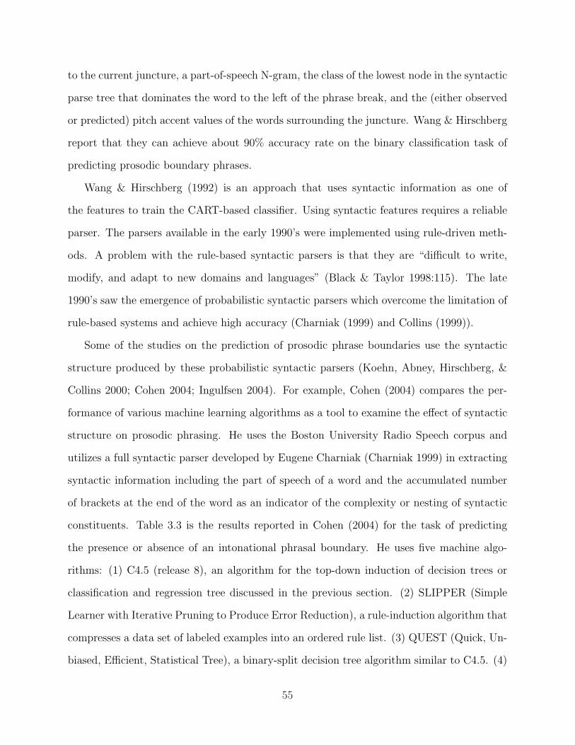
to the current juncture, a part-of-speech N-gram, the class of the lowest node in the syntactic

parse tree that dominates the word to the left of the phrase break, and the (either observed

or predicted) pitch accent values of the words surrounding the juncture. Wang & Hirschberg

report that they can achieve about 90% accuracy rate on the binary classification task of

predicting prosodic boundary phrases.

Wang & Hirschberg (1992) is an approach that uses syntactic information as one of

the features to train the CART-based classifier. Using syntactic features requires a reliable

parser. The parsers available in the early 1990’s were implemented using rule-driven meth-

ods. A problem with the rule-based syntactic parsers is that they are “difficult to write,

modify, and adapt to new domains and languages” (Black & Taylor 1998:115). The late

1990’s saw the emergence of probabilistic syntactic parsers which overcome the limitation of

rule-based systems and achieve high accuracy (Charniak (1999) and Collins (1999)).

Some of the studies on the prediction of prosodic phrase boundaries use the syntactic

structure produced by these probabilistic syntactic parsers (Koehn, Abney, Hirschberg, &

Collins 2000; Cohen 2004; Ingulfsen 2004). For example, Cohen (2004) compares the per-

formance of various machine learning algorithms as a tool to examine the effect of syntactic

structure on prosodic phrasing. He uses the Boston University Radio Speech corpus and

utilizes a full syntactic parser developed by Eugene Charniak (Charniak 1999) in extracting

syntactic information including the part of speech of a word and the accumulated number

of brackets at the end of the word as an indicator of the complexity or nesting of syntactic

constituents. Table 3.3 is the results reported in Cohen (2004) for the task of predicting

the presence or absence of an intonational phrasal boundary. He uses five machine algo-

rithms: (1) C4.5 (release 8), an algorithm for the top-down induction of decision trees or

classification and regression tree discussed in the previous section. (2) SLIPPER (Simple

Learner with Iterative Pruning to Produce Error Reduction), a rule-induction algorithm that

compresses a data set of labeled examples into an ordered rule list. (3) QUEST (Quick, Un-

biased, Efficient, Statistical Tree), a binary-split decision tree algorithm similar to C4.5. (4)

55

Neural Network, also called as Artificial Neural Network (ANN), an algorithm best-known

for its computational attempt to model the cortical structure of the brain. (5) Naıve Bayes

classifier, a simple probabilistic classifier that applies Bayes’ theorem in (3.15):

P (A|B) =P (A)P (B|A)

P (B)(3.15)

See Cohen (2004) for detailed description and references of each algorithm.

Table 3.3: Results of Cohen (2004) on prosodic boundary prediction. Cohen (2004) reportsthe results in terms of training and testing errors, which I convert into accuracy and put inparentheses.

Learner Training Errors (Accuracy) Testing Errors (Accuracy)C4.5 7.6% (92.4%) 11.2% (88.8%)SLIPPER 9.8% (90.2%) 10.2% (89.8%)QUEST 9.7% (90.3%) 11.1% (88.9%)Neural Network 10.1% (89.9%) 10.8% (89.2%)Naive Bayes 11.3% (88.7%) 11.1% (88.9%)

The experimental results in Cohen (2004) indicate two points: First, syntactic con-

stituency is an important feature for prosodic phrasing. Second, given fairly consistent

performance across learning algorithms, it seems that linguistic information may be more

important than the choice of a machine learning algorithm in improving the performance of

the prosodic phrasing prediction.

Ingulfsen (2004) uses a memory-based machine learning algorithm to examine the effect

of various syntactic representations on prosodic phrasing. The Boston University Radio

Speech corpus is used to extract and compare various syntactic representations, including

punctuation marks, the part of speech, the shallow syntactic chunking, and the syntactic

constituents produced by the full syntactic parser developed by Michael Collins (Collins

1999). Ingulfsen concludes that, in predicting prosodic phrasing, the information obtained

56

through the full syntactic parser yields the best performance.

There is a problem in using full syntactic parser, despite the experimental results showing

good performance in the task of prosody phrasing prediction. My own observation on the

output of full syntactic parsers such as Charniak (1999) and Collins (1999) indicates that the

full syntactic parser is error-prone. Again, Black & Taylor (1998) also state that “although

we argued . . . against using syntactic parsers for phrase break assignment, our reasons stem

from the basic inaccuracy of these parsers, not because syntactic parses themselves are

unhelpful. (p. 115)”

As an alternative, Black & Taylor (1998) adopt an alternative approach that uses a

probabilistic method on the part-of-speech (POS) sequences of an utterance. The database

consists of spoken British English mostly read from scripts such as news stories and weather

reports. The number of words used for the POS-based probability estimation is 39,369

and the number of both major and minor prosodic phrase breaks is 7750. Black & Taylor

employ a Markov model to predict probabilities of POS sequences for utterances. In the

model, each state represented either a break or a non-break and the transitions between

states represented the likelihood of particular sequences of breaks and non-break occurring.

Each state had an observation probability distribution giving how likely that state was to

have produced a particular sequence of POS tags. They report that the best setup, which is

6-gram POS sequence, correctly identifies 86.6% of prosodic phrase breaks in the test corpus.

Two levels of prosodic phrasing are usually assumed in the description of prosodic struc-

ture (Ladd 1986). However, it turns out that correct classification of the two levels of

prosodic phrasing is quite difficult to make. Ingulfsen (2004) conducted a series of experi-

ments predicting levels of prosodic phrasing in addition to the above-mentioned prediction of

binary prosodic boundary location. He reports that with the best setting obtained through

the full-syntactic parsing, the best performance achieves precision rate of 74.9% and recall

rate of 77.9% in identifying break index 4 (or intonational phrase). As for the correct iden-

tification of break index 3 (or intermediate phrase), only recall rate of 0.56% and precision

57

rate of 42.9% are achieved.

Ross & Ostendorf (1996) report on the experiment of predicting types of boundary tones

such as L-L% or L-H% on the Boston University Radio Speech corpus. Various features

are used including the number of syllables and the location of lexical stress, among others.

But as far as syntactic information is concerned, only part of speech is used as a feature,

with no higher level of syntactic information such as syntactic constituency. Table 3.4 is a

confusion matrix regarding the types of boundary tone. The number of words used for the

experiment is 8841 words (or 48minutes of recorded speech), and 1904 words (or about 20%

of the data) are used for testing, while the rest 6937 words are used for training. It should

be noted, however, that the domain of prediction task is not on the basis of word, but on

the basis of syllable. Other boundary types such as H-H% are not reported due to the lack

of observation in the corpus.

Table 3.4: Confusion matrix that shows the results of types of prosodic boundary in Ross& Ostendorf (1996). The classification is done under the assumption that the prosodicboundary location is already known. Note that words that are not associated with prosodicboundary are not included for calculation, the overall accuracy is reported to be lower.

PredictedObserved L-L% H-L% L-H% Recall

L-L% 220 0 19 92.05%H-L% 12 0 4 0.00%L-H% 97 0 39 28.67%

Precision 66.86% 0.00% 62.90% 66.24%

Note that the overall accuracy of 66.24% is calculated with no reference to the no bound-

ary condition, where the syllable under investigation does not bear any intonational phrase

boundary. Ross & Ostendorf (1996) filter out those syllables that does not bear the in-

tonational boundary, and then calculated the recall rate. Otherwise, the overall accuracy

would be reported to be higher than the rather poor 66.24%. They report that about 90%

of accuracy is achieved in correctly predicting a syllable with no prosodic boundary.

The earlier studies demonstrate that the presence of a prosodic boundary can be predicted

58

with a fair degree of accuracy. They also reveal a limitation of corpus-based machine learning

algorithms. The accuracy rate can drop to zero in the case where not enough training tokens

are available in the database, such as H-L% and H-H% as shown in the study of Ross &

Ostendorf (1996). The sparseness of the data is, in a sense, related to the characteristics of

the corpus. For example, the boundary type of H-H% is expected to be observed in a corpus

that contains many questions, but the type is not expected much in a corpus like the radio

speech corpus in which questions are rarely observed.

3.4.2 Prosodic prominence prediction

Like the task of prosodic phrasing prediction, various experimental set-ups can be designed

from binary classification of the presence vs. absence of pitch accent to multi-class classifi-

cation of predicting types of pitch accent.

Predicting prosodic prominence is more difficult than predicting prosodic phrasing, be-

cause the determination of prosodic prominence is influenced by semantic and pragmatic

factors in addition to phonological and syntactic factors. The semantic and pragmatic fac-

tors are extremely hard to extract automatically from the text alone. Nevertheless, earlier

studies shed lights on the relevant factors to the task of prosodic prominence prediction.

Many features are found to be useful in accent prediction, including the part of speech of

a word (Hirschberg 1993; Cohen 2004), informativeness of a word (Pan & McKeown 1999),

and various measures of word probability (Ross & Ostendorf 1996, Yuan et al. 2005), among

others.

Hirschberg (1993) uses a binary decision tree to automatically predict the presence or

absence of pitch accent in a word of an utterance from a number of databases, including

read materials from an FM radio speech corpus, which was later released as the Boston

University Radio Speech corpus. The features used in the decision tree design include word

class context (i.e., broad classes of part-of-speech labels such as function words and content

words), the stress location in the compound nominals (Sproat 1994), the position of the word

59

Table 3.5: Results of Cohen (2004) on pitch accent prediction using features obtained fromfull Charniak parser data. Cohen (2004) reports the results in terms of training and testingerrors, which I have converted into accuracy and put in the parenthesis.

Learner Training Errors (Accuracy) Testing Errors (Accuracy)C4.5 14.6% (85.4%) 17.8% (82.2%)SLIPPER 17.3% (82.7%) 17.7% (82.2%)QUEST 17.5% (82.5%) 17.4% (82.6%)Neural Network 17.2% (82.8%) 17.1% (82.9%)Naive Bayes 22.1% (77.9%) 21.7% (78.2%)

within an intonational phrase and utterance, and the length of the utterance containing the

word, speaker identity, and simple discourse information such as new or given status of the

word. Here, ‘new’ vs. ‘given’ is computed as a simple stack algorithm for a given word. If a

word is saved in the memory for the first time, then the word is labeled ‘new’, and the word

appears again later in the paragraph, then the word is labeled as ‘old.’ The cross-validated

accuracy rate is reported to be 76.5% for predicting the presence or absence of pitch accent

on the FM news stories. Interestingly, the predicted tree produced for this data set consists

of only a single split. The split is based on the distinction of the function word and the

content word. One reason for this single split is that “the classification procedure simply

had too little data to make generalizable predictions for this corpus” (Hirschberg 1993:328).

Nevertheless, Hirschberg (1993) shows the importance of the distinction of the word classes

into content words and function words in the predictive task of pitch accent.

Cohen (2004) along with other studies also confirms the importance of the part of speech

information in predicting the presence or absence of pitch accent. He concludes that “use

of part of speech information alone is sufficient to achieve fairly high accuracy on predict-

ing word accentuation,” based on prediction experiments using numerous machine learning

algorithms. The range of accuracy in the task is reported to be 78.2% to about 82.9%, as

60

shown in Table 3.4.

Usefulness of Information Content (IC) of words is investigated by Pan & McKeown

(1999). Following the standard definition in information theory, the information content

(IC) of a word is calculated as the negative log probability of a word,

IC(ω) = − log(P (ω))

= − log

(F (ω)

N

)(3.16)

where P (ω) is the probability of the word ω appearing in a corpus and P (ω) is estimated as

F (ω)N

, where F (ω) is the frequency of ω in the corpus and N is the total number of word tokens

in the corpus. Intuitively, if the probability of a word increases, its informativeness decreases.

It is, therefore, less likely to be communicated with pitch prominence. Pan & McKeown

(1999) demonstrate that the information content is inversely proportional to the probability

of the word’s accentuation, when the IC is tested on a corpus of doctors’ prescription or

diagnosis collected in a hospital. Despite its intuitive appeal, the measurement of IC doesn’t

seem to be relevant in the Boston University Radio Speech corpus. Yuan, Jason & Jurafsky

(2005) show experimental results of binary classification of the presence/absence of a pitch

accent. The experiment is done using the decision tree package C4.5 (Quinlan 1986) with

10-fold cross validation. The following features are extracted: 1) the part of speech of a word

in an utterance, 2) the unigram probability of a word, 3) the bigram probability of a word,

4) the backward bigram probability of a word, 5) the position of the word in an intonational

phrase, 6) the Information Content (IC) of the word, and finally 7) the accent ratio of a

word over the corpus. In Yuan et al. (2005), the accent ratio is defined as ‘the number of

accented tokens of a word divided by the total number of tokens of that word in the corpus’.

The part of speech, the unigram probability, and the backward bigram probability are useful

features for pitch accent prediction. However, the IC of the word doesn’t contribute much

61

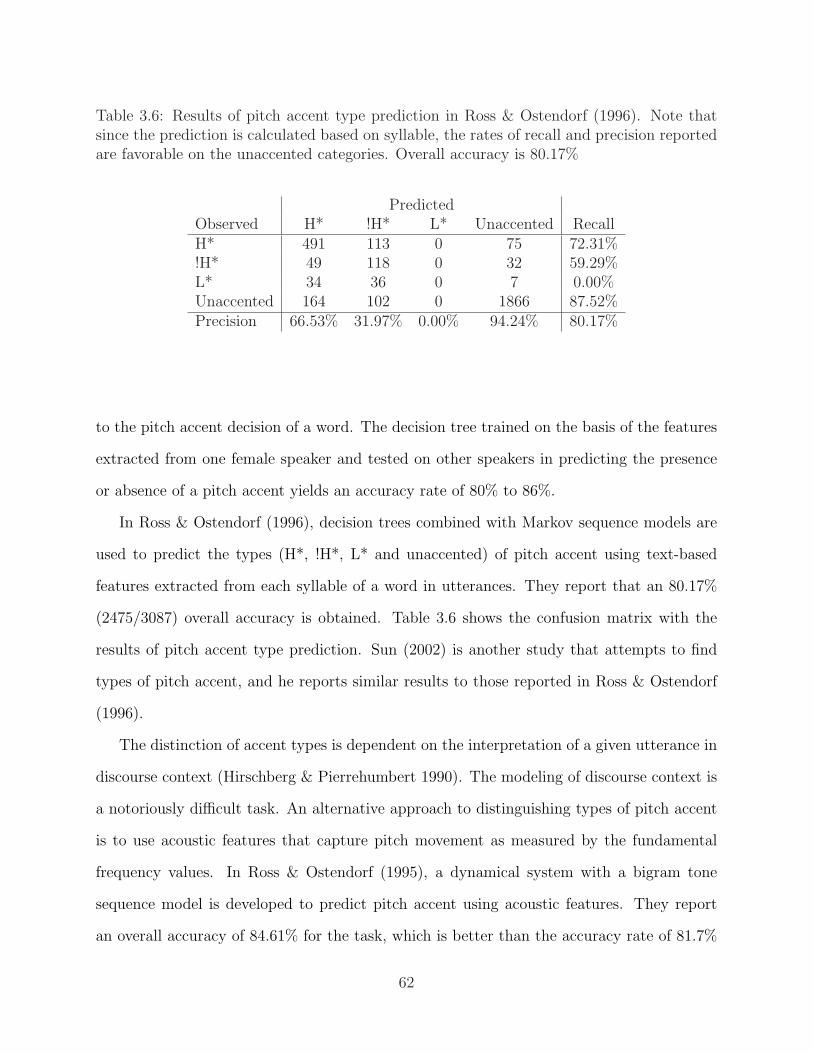
Table 3.6: Results of pitch accent type prediction in Ross & Ostendorf (1996). Note thatsince the prediction is calculated based on syllable, the rates of recall and precision reportedare favorable on the unaccented categories. Overall accuracy is 80.17%

PredictedObserved H* !H* L* Unaccented RecallH* 491 113 0 75 72.31%!H* 49 118 0 32 59.29%L* 34 36 0 7 0.00%Unaccented 164 102 0 1866 87.52%Precision 66.53% 31.97% 0.00% 94.24% 80.17%

to the pitch accent decision of a word. The decision tree trained on the basis of the features

extracted from one female speaker and tested on other speakers in predicting the presence

or absence of a pitch accent yields an accuracy rate of 80% to 86%.

In Ross & Ostendorf (1996), decision trees combined with Markov sequence models are

used to predict the types (H*, !H*, L* and unaccented) of pitch accent using text-based

features extracted from each syllable of a word in utterances. They report that an 80.17%

(2475/3087) overall accuracy is obtained. Table 3.6 shows the confusion matrix with the

results of pitch accent type prediction. Sun (2002) is another study that attempts to find

types of pitch accent, and he reports similar results to those reported in Ross & Ostendorf

(1996).

The distinction of accent types is dependent on the interpretation of a given utterance in

discourse context (Hirschberg & Pierrehumbert 1990). The modeling of discourse context is

a notoriously difficult task. An alternative approach to distinguishing types of pitch accent

is to use acoustic features that capture pitch movement as measured by the fundamental

frequency values. In Ross & Ostendorf (1995), a dynamical system with a bigram tone

sequence model is developed to predict pitch accent using acoustic features. They report

an overall accuracy of 84.61% for the task, which is better than the accuracy rate of 81.7%

62

Table 3.7: Results of pitch accent prediction using both acoustic and text features withAdaBoost CART in Sun (2002). Note that since the prediction is calculated based onsyllable, the rates of recall and precision reported are favorable on the unaccented categories.

PredictedObserved H* !H* L* Unaccented RecallH* 565 48 1 63 83.46%!H* 106 51 3 51 24.17%L* 2 0 3 30 8.57%Unaccented 49 9 4 1967 96.79%Precision 78.25% 47.22% 27.27% 93.17% 87.60%

achieved through the text-based features. Sun (2002) designs an experimental setting of

predicting accent types using both textual and acoustic information extracted based on the

syllable-based domain in each word. The data is divided into 80% of traing and 20% of

test data. Table 3.7 shows the confusion matrix of the accent type prediction task obtained

through both acoustic and textual features. Sun (2002) uses AdaBoost CART, and the

AdaBoost CART refers to the CART trained with a boosting algorithm called AdaBoost.

Simply speaking, boosting is a way of reducing prediction error of a classifier by lowering bias

and variance. See Sun (2002:49-51) for the motivation of combining the base CART learner

with a boosting. In comparison, Table 3.8 shows the confusion matrix obtained through

only textual features. In general, using combined features both from acoustic signals and

textual features shows an improved performance in the task.

3.5 Conclusion

Probabilistic approaches are more suitable than deterministic approaches in describing and

modeling prosodic structure. Machine learning algorithms are data-driven and possess at-

tractive characteristics and are widely used in many areas of natural language and speech

63

Table 3.8: Results of pitch accent prediction using text features with AdaBoost CART inSun (2002). Note that since the prediction is calculated based on syllable, the rates of recalland precision reported are favorable on the unaccented categories.

PredictedObserved H* !H* L* Unaccented RecallH* 482 32 0 163 72.53%!H* 121 35 1 55 19.43%L* 25 3 0 7 0.0%Unaccented 120 26 0 1783 91.45%Precision 64.43% 36.45% 0.00% 88.79% 80.61%

processing. In this chapter, I reviewed two such algorithms, MBL and CART, that are suc-

cessfully and widely used in many research areas, followed by standard evaluation metrics

that are typically employed in evaluating the performance of machine learning algorithms.

I mentioned that among various algorithms, I chose to review these two algorithms due

to their flexibility and efficiency in dealing with both continuous and categorical variables.

Finally, I reviewed earlier predictive studies of prosodic structure.

In the next two chapters, I present experimental studies of prosodic structure prediction

by using a machine learning algorithm on linguistic features extracted from texts (Chapter

4), on acoustic features extracted from speech sounds, and on both the linguistic and acoustic

features (Chapter 5).

64

Chapter 4

Predictive Models of Prosody throughGrammatical Interface

4.1 Introduction

This chapter reports on experiments predicting pitch accents and boundary tones using

linguistic features extracted from an utterance. In the previous chapter, I reviewed memory-

based learning algorithm, and Classification and Regression Tree, both of which are flexible

and efficient in dealing with both continuous and categorical variables. In this chapter

I confine my presentation to the memory-based machine learning experiments. Memory-

based machine learning is applied to the extracted features. After describing the motivation

for choosing each feature, I illustrate the way the feature is extracted from the grammatical

components of syntax, phonology, and semantic or discourse structure. Finally, I present

results on the prediction tasks of prosodic structure.

Features are extracted from the labnews portion of the Boston University Radio Speech

corpus by automatic tagging or by dictionary lookup. To reiterate, the Boston Radio Speech

corpus is a speech corpus produced by professional FM Radio News announcers (3 female

and 2 male speakers). The corpus is prosodically labeled using the ToBI annotation system.

Besides the words and prosody labels, the corpus also includes texts containing the news

scripts and pronunciation dictionary. The total number of word tokens collected for this

project is about 10,000 and the number of sentence tokens is about 600. Each sentence has,

on average, 16 words. Note that because the speakers produced the same news scripts, the

number of word types is quite limited. About 900 word types are found in the radio speech

corpus.

65

4.2 Feature Extraction

Linguistically motivated features are extracted automatically or using a dictionary look-up.

4.2.1 Syntactic features

Syntactic features encoding the part of speech of a word, and the shallow syntactic phrase

structure are automatically extracted using the shallow parser developed by the Inductive

Linguistic Knowledge (ILK) group of the University of Tilburg and available at the ILK

webpage http://ilk.kub.nl.

Part of Speech

Traditionally, grammatical theory has recognized the syntactic categories of noun, verb, ad-

jective, adverb, pronoun, preposition, conjunction, and interjection. From a psychological

vantage point, these categories may be placed into two groups. Open-class words (sometimes

called content words) include nouns, verbs, adjectives, and adverbs. Closed-class words (also

called function words) include determiners, pronouns, prepositions, conjunctions and inter-

jections.1 From a linguistic vantage point, open-class words are more likely to encode entities

and activities that are newly introduced in a discourse, or the attributes of those entities

or activities. Thus, it is more likely that prosodic prominence is correlated with open-

class words than closed-class words, a prediction that is empirically confirmed by Wang &

Hirschberg (1992), Hirschberg (1993), Veilleux (1994), Ross & Ostendorf (1996), Taylor &

Black (1998), Cohen (2004), Ingulfsen (2004), Yuan et al. (2005), among others. Further-

more, the part of speech information is a necessary prerequisite for higher level syntactic

tagging, including shallow or full syntactic parsing, semantic role or argument structure

tagging, and named entity tagging, as discussed below.

1For example, people suffering from agrammatism frequently omit closed-class words and inflectionalendings from their utterance of sentence, while preserving open-class words somewhat better (Bradley,Garrett, & Zurif 1980).

66

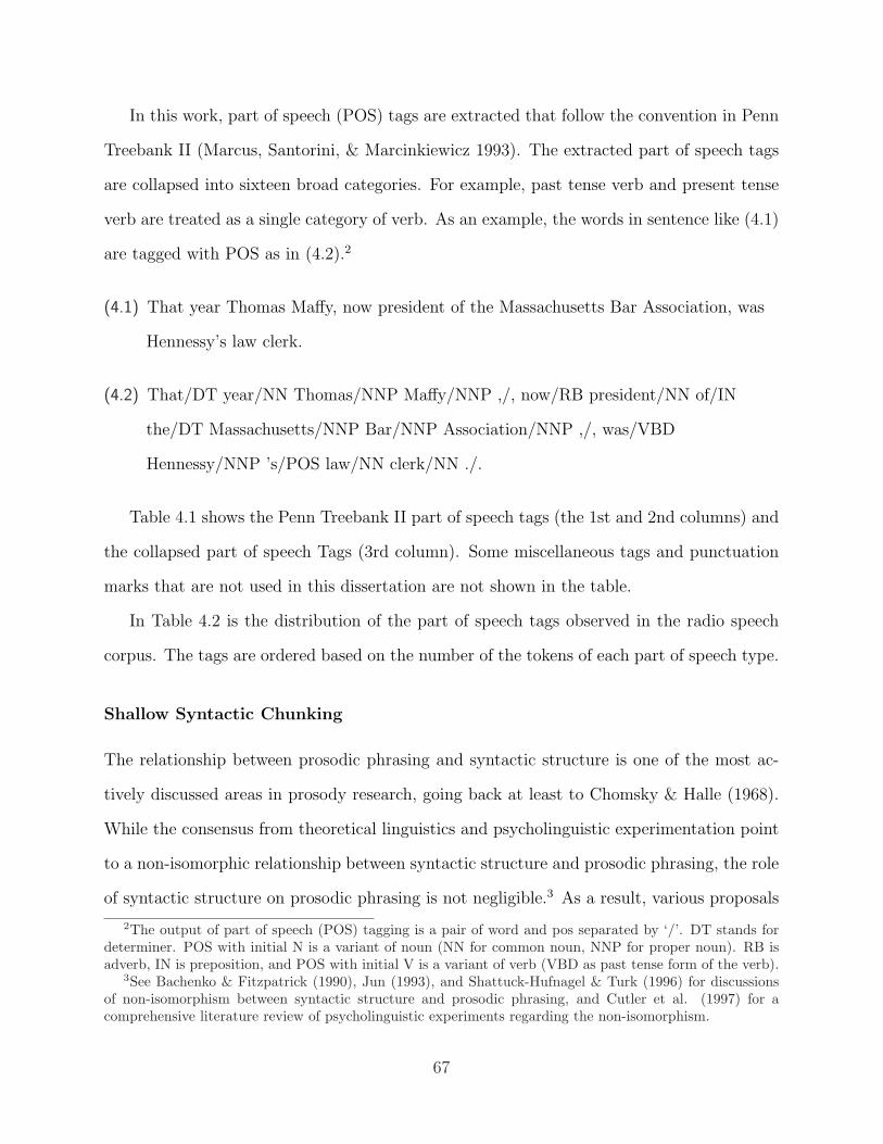
In this work, part of speech (POS) tags are extracted that follow the convention in Penn

Treebank II (Marcus, Santorini, & Marcinkiewicz 1993). The extracted part of speech tags

are collapsed into sixteen broad categories. For example, past tense verb and present tense

verb are treated as a single category of verb. As an example, the words in sentence like (4.1)

are tagged with POS as in (4.2).2

(4.1) That year Thomas Maffy, now president of the Massachusetts Bar Association, was

Hennessy’s law clerk.

(4.2) That/DT year/NN Thomas/NNP Maffy/NNP ,/, now/RB president/NN of/IN

the/DT Massachusetts/NNP Bar/NNP Association/NNP ,/, was/VBD

Hennessy/NNP ’s/POS law/NN clerk/NN ./.

Table 4.1 shows the Penn Treebank II part of speech tags (the 1st and 2nd columns) and

the collapsed part of speech Tags (3rd column). Some miscellaneous tags and punctuation

marks that are not used in this dissertation are not shown in the table.

In Table 4.2 is the distribution of the part of speech tags observed in the radio speech

corpus. The tags are ordered based on the number of the tokens of each part of speech type.

Shallow Syntactic Chunking

The relationship between prosodic phrasing and syntactic structure is one of the most ac-

tively discussed areas in prosody research, going back at least to Chomsky & Halle (1968).

While the consensus from theoretical linguistics and psycholinguistic experimentation point

to a non-isomorphic relationship between syntactic structure and prosodic phrasing, the role

of syntactic structure on prosodic phrasing is not negligible.3 As a result, various proposals

2The output of part of speech (POS) tagging is a pair of word and pos separated by ‘/’. DT stands fordeterminer. POS with initial N is a variant of noun (NN for common noun, NNP for proper noun). RB isadverb, IN is preposition, and POS with initial V is a variant of verb (VBD as past tense form of the verb).

3See Bachenko & Fitzpatrick (1990), Jun (1993), and Shattuck-Hufnagel & Turk (1996) for discussionsof non-isomorphism between syntactic structure and prosodic phrasing, and Cutler et al. (1997) for acomprehensive literature review of psycholinguistic experiments regarding the non-isomorphism.

67

Table 4.1: Penn Treebank II part of speech tags. The POS tags are collapsed into sixteenbroad categories. Note that I made possessive ending ’s (indicated with *) attached to thepreceding noun and treated the noun and possessive together as a noun.

Abbreviated Full CollapsedPOS name POS name POS name

CC Coordinating Conjunction ConjunctCD Cardinal number NumeralDT Determiner DeterminerEX Existential “there” Existential thereIN Preposition or Subordinating conjunction PrepositionJJ Adjective Adjective

JJR Adjective, comparative AdjectiveJJS Adjective, superlative AdjectiveMD Modal ModalNN Noun, singular or mass Noun

NNS Noun, plural NounNNP Proper noun, singular Noun

NNPS Proper noun, plural NounPDT Predeterminer PredeterminerPOS Possessive ending* NounPRP Personal pronoun Pronoun

PRP$ Possessive pronoun PronounRB Adverb Adverb

RBR Adverb, comparative AdverbRBS Adverb, superlative AdverbRP Particle ParticleTO “to” Infinitive toUH Interjection InterjectiveVB Verb, base form Verb

VBD Verb, past tense VerbVBG Verb, gerund or present participle VerbVBN Verb, past participle VerbVBP Verb, non 3rd-person singular present VerbVBZ Verb, 3rd person singular present Verb

WDT Wh-determiner Wh-WordsWP Wh-pronoun Wh-Words

WP$ Possessive wh-pronoun Wh-WordsWRB Wh-adverb Wh-Words

68

Table 4.2: Distribution of Parts of Speech in the radio news speech corpus

Part of Speech Number of tokens ProportionNoun 3454 32.7%Verb 1700 16.1%Preposition 1282 12.1%Determiner 1046 9.9%Adjective 870 8.2%Pronoun 490 4.6%Adverb 412 3.9%Infinitive to 330 3.12%Conjunct 294 2.7%Numeral 273 2.5%Modal 196 1.8%Wh-Words 118 1.1%Particle 47 0.4%Interjective 15 0.1%Existential there 11 0.1%Predeterminer 10 0.09%

have been advanced for the proper treatment of syntactic structure and prosodic phras-

ing. The proposals include deriving prosodic structure from a flattened syntactic structure

(Chomsky & Halle 1968; Langendoen 1976), a mapping rule to convert from syntactic to

prosodic structure (Cooper & Paccia-Cooper 1980; Nespor & Vogel 1986), constraints that

mediate between syntactic and prosodic structure (Taglich 1998; Selkirk 2000), deriving

prosodic structure in relation to information structure or surface syntactic structure (Steed-

man 2000), and a proper probabilistic mapping between prosodic and syntactic structure

(Wang & Hirschberg 1992; Veilleux 1994; Ross & Ostendorf 1996; Koehn et al. 2000; Cohen

2004; Chen 2004, and Ingulfsen 2004).

The common assumption behind these various approaches is that prosodic phrasing is

constrained first and foremost by syntactic constituency. (Of course, not every syntactic

constituent forms a prosodic phrase). Therefore, it is desirable to parse the full syntactic

structure and investigate the correlation between syntactic structure and prosodic phrasing.

69

There are, however, at least two practical drawbacks in using automatic parsing of full

syntactic structure. The most problematic issue is the inaccuracy of the full syntactic parse,

despite advancement of the parsing technology. My own experience in using full syntactic

parsers (Collins 1999; Charniak 1999) confirms the comment made by Taylor & Black (1998)

that the accuracy of full syntactic parsing is problematic for the development of syntax-

dependent prosodic models. The second is the assumption of deterministic output of the

full syntactic parser with probabilistic ambiguity resolution. For example, even though the

phrase “I saw the man with a telescope.” is structurally ambiguous between “I saw the man

using the telescope.” and “I saw the man who has the telescope.”, the deterministic nature

of the parser cranks out only one out of the competing structures.

To overcome the inaccuracy and deterministic nature of full syntactic parser, I rely on

the intermediate syntactic structure called shallow syntactic parsing, or shallow chunking.

The syntactic chunks are non-overlapping and non-embedded constituents (Punyakanok &

Roth 2001; Buckholz 2002),4 and are in some way similar to the flattened syntactic structure

proposed by Chomsky & Halle (1968) and Langendoen (1976) for the mapping of syntactic

structure to prosodic phrasing. An example of the shallow syntactic parsing of the sentence

in (4.1) is shown in (4.3).5

(4.3) [ NP1 That/DT year/NN Thomas/NNP Maffy/NNP NP1 ] ,/, [ ADVP now/RB

ADVP ] [ NP president/NN NP ] { PNP [ P of/IN P ] [ NP the/DT

Massachusetts/NNP Bar/NNP Association/NNP NP ] PNP } ,/, [ VP1 was/VBD

VP1 ] [ NP1 Hennessy/NNP ’s/POS law/NN clerk/NN NP1 ] ./.

Even though the overall accuracy of the shallow parser is better than that of a full

syntactic parser, the shallow parser is not 100% accurate. Note the inaccurate parsing of

4Buckholz (2002) contains a comprehensive literature review on syntactic parsing technology.5The output of shallow parsing is marked next to the open-closed angled brackets ([]) or curly brackets

({}). Thus, the domain of the chunking is from the open bracket to the closing bracket. The curly bracketsare used when a smaller phrase is nested within a larger phrase. For example, Prepositional Phrase (P) isnested within PNP (Prepositional Noun Phrase). NP stands for Noun Phrase; ADVP for Adverbial Phrase;VP for verbal phrase. The number 1 indicates the dependence of the phrase on the verb.

70

Table 4.3: Distribution of shallow syntactic chunks in the radio speech corpus

Syntactic chunking Number of tokens ProportionNoun Phrase (NP) 6267 59.4%Verb Phrase (VP) 2180 20.6%Prepositional Phrase (PP) 1164 11.0%Conjunction (ConjP) 280 2.6%Adverbial Phrase (ADVP) 202 1.9%Adjectival Phrase (ADJP) 175 1.6%Particle (PRT) 48 0.4%Interjective 19 0.1%NEG 26 0.2%Complementizer 187 1.7%

Table 4.4: Distribution of chunking size of the shallow parser in the corpus

Chunking size Number of tokens Proportion1 6566 62.2%2 2452 23.2%3 1001 9.4%4 350 3.3%5 127 1.2%6 37 0.3%7 10 0.09%8 5 0.04%

“That year Thomas Maffy” as a Noun Phrase. I will discuss how to remedy the inaccuracy

of the output below.

Table 4.3 shows the distribution of the shallow syntactic chunks and Table 4.4 shows the

distribution of the chunking size.

4.2.2 Phonological features

The number of phones, number of syllables, and position of primary stress within each

word are extracted using dictionary lookup. The Boston University Radio Speech corpus

is accompanied by lexicon files that contain pronunciation, a syllable boundary markers,

71

and location of stress. For the sake of simplicity, I used the lexicon files to define these

phonological features. The need for phonological features in prosody prediction is motivated

by the observation that the mismatch between syntactic structure and phonological phrasing

is often affected by nonsyntactic factors such as the length of a phrase for placement of

prosodic phrase boundaries and pitch-accent, or word frequency for placement of phrasal

pitch-accent, as stated in Bachenko & Fitzpatrick (1990) and evidenced in Gee & Grosjean

(1983). Phonological length, or heaviness, plays a role in both syntax and prosody. However,

it is not clear how phonological length is measured (Fitzpatrick 2001), or to what extent

phonological length contributes to the determination of prosodic prominence or prosodic

phrasing.

It is noted in earlier literature that the number of syllables may play a role in prosodic

phrasing. Bierwisch (1966; cited in Bachenko & Fitzpatrick 1990) takes the number of

syllables as a factor in affecting prosodic phrasing. Rice (1987) also considers the syllable as

an appropriate measure of length.

The reason for establishing some abstract notion of length, whatever the proper unit is, is

expressed in Nespor & Vogel (1986), who take note of a tendency to make each intonational

phrase a more or less uniform length, even though it is uncertain how to characterize the more

or less ideal length precisely (p. 194). The resulting rhythmic patterns of roughly uniform

length, in which some elements are distinguished from others, facilitate the encoding of

linguistic information into the signal by the speaker and the decoding of that information

out of the signal by the listener (Aylett 2000; Martin 1972).

Thus, in this project, I extract the phonological features of the number of phones, (Table

4.5) and the number of syllables (Table 4.6) of each word in an utterance, and the position of

primary stress (Table 4.7) within a word by using dictionary lookup method. The dictionary

presents the typical or canonical phonetic representation of a word, and as such will in some

instances be at odds with the phonetic form of a particular word token, but the advantage of

the dictionary form is that it can be obtained without relying on an accurate segmentation

72

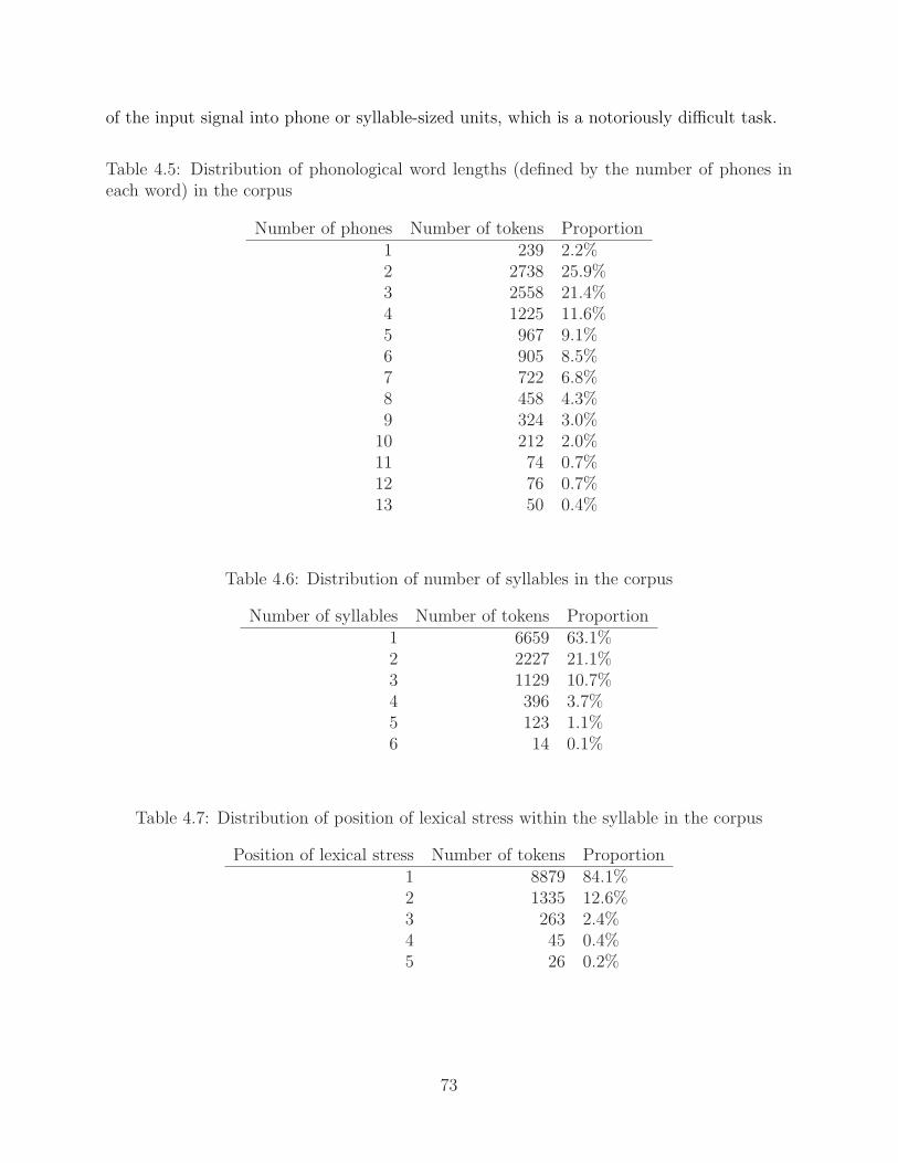
of the input signal into phone or syllable-sized units, which is a notoriously difficult task.

Table 4.5: Distribution of phonological word lengths (defined by the number of phones ineach word) in the corpus

Number of phones Number of tokens Proportion1 239 2.2%2 2738 25.9%3 2558 21.4%4 1225 11.6%5 967 9.1%6 905 8.5%7 722 6.8%8 458 4.3%9 324 3.0%

10 212 2.0%11 74 0.7%12 76 0.7%13 50 0.4%

Table 4.6: Distribution of number of syllables in the corpus

Number of syllables Number of tokens Proportion1 6659 63.1%2 2227 21.1%3 1129 10.7%4 396 3.7%5 123 1.1%6 14 0.1%

Table 4.7: Distribution of position of lexical stress within the syllable in the corpus

Position of lexical stress Number of tokens Proportion1 8879 84.1%2 1335 12.6%3 263 2.4%4 45 0.4%5 26 0.2%

73

4.2.3 Semantic features

Argument structure (or predicate-argument relations) and named entities are automatically

extracted. The predicate-argument relation is extracted from the same package used for part-

of-speech tagging and shallow syntactic tagging. Named entities are tagged by using NEPack-

ages developed by UIUC Cognitive Computing Group, i.e., http://l2r.cs.uiuc.edu (Kle-

mentiev & Roth 2006).

Predicate-argument relations

Predicate-argument relations (or argument structure) have been proposed for their possible

effect on prosodic phrasing. Crystal (1969) claims that prosodic boundaries will co-occur

with grammatical functions such as subject, predicate, modifier, and adjunct. Selkirk’s

(1984) ‘sense unit condition’ on prosodic phrasing can be interpreted to group arguments

with a predicate. She states that immediate constituents of an intonational phrase must

together form a sense unit. Formally, a sense unit is formed if a constituent (Ci ) modifies

a head (Cj ) or if a constituent (Ci) is an argument of a head (Cj)6. According to the

condition, for example, in a subject, verb and object construction, either a subject and a

verb can form a unit or a verb and an object can form a unit. Let’s consider a sentence

“Mary prefers corduroy” is produced with two intonational phrase as in “(Mary prefers)IP

(corduroy)IP.” The first intonational phrase “(Mary prefers)IP” does not correspond to one

syntactic constituent, as the syntactic representation in (4.4) shows.

6In Selkirk (1984:291), the sense unit condition on intonational phrasing is formally expressed as follows:“Two constituents Ci, Cj form a sense unit if (a) or (b) is true of the semantic interpretation of the sentence.”(a) Ci modifies Cj (a head) (b) Ci is an argument of Cj (a head)

74

(4.4) S

©©©©HHHH

NP

Mary

VP

V

©©©HHH

prefers NP

Corduroy

Nevertheless, the two constituents in the intonational phrase stand in the relation of

argument-head, since the NP ‘Mary ’ is an argument of verb ‘prefers ’. Thus they form a

sense group and can license the intonational phrase. Alternatively, the same sentence “Mary

prefers corduroy” may be produced as in “(Mary)IP (prefers corduroy)IP.” Once again, the

second intonational phrase ‘(prefers corduroy)’ IP has its two constituents in the relation of

head-argument (i.e., verb ‘prefers ’ and object ‘corduroy ’). Therefore, the sense unit condition

is closely related to argument structure.

Bachenko, Fitzpatrick, & Wright (1986) also assume that phrasing is dependent on

predicate-argument structure. Despite these claims, the argument in favor of the role of

predicate-argument structure on prosodic phrasing has drawn less attention in the predic-

tion of prosodic structure than the argument in favor of the role of syntactic structure. The

disregard for argument structure is directly acknowledged, e.g., “the prosodic phrasing in

observed data often ignores the argument status of constituents (Bachenko & Fitzpatrick

1990:157).” Nevertheless, argument structure features such as subject, object and predicate

aid in categorizing the shallow syntactic chunks into their relevant grammatical roles. Ar-

gument structure is also helpful in identifying parenthetic phrases, which are acknowledged

to be an important factor in grouping of prosodic phrasing (Taglich 1998; Selkirk 1995). For

example, Selkirk states that the parenthetical phrase forms an intonational phrase. Paren-

75

thetical phrases cause errors quite often in full syntactic parsing.7 Example (4.5) illustrates

the output of predicate-argument tagging, and the distribution of the predicate-argument

relations (or grammatical roles) are in Table 4.8. Note that due to the initial error in shallow

syntactic tagging, the first noun phrase (NP) is tagged as a subject.8

(4.5) [ NP1Subject That/DT year/NN Thomas/NNP Maffy/NNP NP1Subject ] ,/, [

ADVP now/RB ADVP ][ NP president/NN NP ] {PNP [ P of/IN P ] [ NP the/DT

Massachusetts/NNP Bar/NNP Association/NNP NP ] PNP } ,/, [ VP1 was/VBD

VP1 ] [ NP1NP-PRD Hennessy/NNP ’s/POS law/NN clerk/NN NP1NP-PRD ] ./.

Table 4.8: Distribution of grammatical roles in the corpus

Grammatical roles Number of tokens ProportionNo Grammatical Roles 5528 52.4%

Subject 1610 15.2%Verb 1911 18.1%

Object 1263 11.9%NP Predicate 200 1.8%Temporal NP 21 0.1%

Wh-NP 10 0.09%Adverbial NP 5 0.04%

Named entity tagging

Named entities are phrases that contain the name of persons, organizations, locations, etc.

As mentioned earlier, shallow syntactic tagging achieves better accuracy over full syntactic

tagging that can be extracted from parsers developed by Collins (1999) or Charniak (1999).

Nevertheless, informal observation of the shallow syntactic tagging reveals regions where

tagging errors are made. By using the named entity tag together with shallow syntactic

parsing, I hypothesize that the accuracy of shallow syntactic tagging can become higher.

7See McCawley (1982) for the theoretical issues in syntactic parsing.8The boldfaced Subject and NP-PRD (Noun Phrase Predicate) denote the grammatical roles or arguments

of the copular verb ‘was’.

76

Besides, the name of persons or organizations is expected to carry higher Information Content

(IC) than corresponding pronouns (e.g., Thomas Maffy vs. he). Example (4.6) illustrates

how named entities are identified and grouped,9 and the distribution of the named entities is

in Table 4.9.10 Four types of named entities are recognized: the name of a person, the name

of an organization, the name of a location, and a miscellaneous name. The distribution

of the word location within a bracket enclosing the named entity is in Table 4.10. Note

that unlike the output of shallow syntactic and argument structure parsing, “That year and

Thomas Maffy” are correctly separated.

(4.6) That year , [PER Thomas Maffy ] , now president of the [LOC Massachusetts ] Bar

Association , was [PER Hennesy ] ’s law clerk .

Table 4.9: Distribution of named entities in the corpus

Named entity Number of tokens ProportionPerson 410 3.8%

Organization 253 2.3%Location 112 1.0%

Miscellaneous 71 0.6%No named entities 9702 91.9%

Table 4.10: Distribution of the location of a word within the brackets to which the wordcomprising the named entity belongs

Brackets Number of tokens ProportionB (Beginning) 250 2.3%

I (Inside) 70 0.6%L (Ending) 250 2.3%

U (Unique, or one-word) 273 2.5%No bracket 9705 91.9%

9PER stands for person, and LOC stands for location.10As mentioned above, named entities are obtained by using NEPackages developed by UIUC Cognitive

Computing Group, i.e., http://l2r.cs.uiuc.edu. See Punyakanok & Roth (2001), and Klementiev & Roth2006 for the description of tagging of named entities.

77

4.3 Integration of the Extracted Features

The features discussed in the previous section are extracted either automatically or using

a dictionary. The automatic extraction is done on the basis of part of speech tags, shallow

syntactic tags, predicate-argument tags, and named entity tags. The dictionary accompanied

by the corpus is used to determine the number of syllables, the number of phones and the

position of primary stress of each word.

In order to train a machine learning algorithm, the extracted features are aligned in a

matrix format, as shown in Table 4.11. Table 4.11 is an example of extracted features of a

sample sentence “That year Thomas Maffy, now president of Massachusetts Bar Association,

was Hennessy’s law clerk.” In addition to the features already mentioned, some additional

features appear in this table, such as the position of a word relative to the end of the sentence

(i.e., in reverse word order), and the cardinal number of the shallow syntactic chunk that

contains the word, again in reverse order, both of which offer a measure of the distance

between the word and the end of the phrase. There is also a feature that encodes the

bracketing information from the named entity tagging.

In Table 4.11, the columns represent (1) Word, (2) Position of the word in the sentence in

decreasing order, (3) Number of syllables in the word, (4) Number of phones in the word, (5)

Position of the primary stress within the word, (6) Part of the Speech of the word, (7) The

type of syntactic phrase containing the word, (8) Position of the word from the end of the

syntactic phrase (phrase-reverse order), (9) the Grammatical Relation of the word, (10) the

type of Named Entities containing the word (null if the word is not part of a named entity),

and (11) Brackets of the Named Entities which the word belongs to. Sentence internal

punctuation is not considered as a feature. At the end of each sentence, # was padded to

mark the sentence boundary.

78

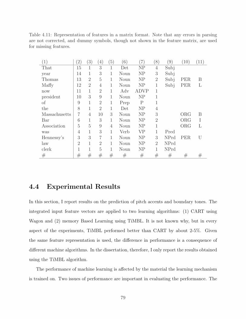
Table 4.11: Representation of features in a matrix format. Note that any errors in parsingare not corrected, and dummy symbols, though not shown in the feature matrix, are usedfor missing features.

(1) (2) (3) (4) (5) (6) (7) (8) (9) (10) (11)That 15 1 3 1 Det NP 4 Subjyear 14 1 3 1 Noun NP 3 SubjThomas 13 2 5 1 Noun NP 2 Subj PER BMaffy 12 2 4 1 Noun NP 1 Subj PER Lnow 11 1 2 1 Adv ADVP 1president 10 3 9 1 Noun NP 1of 9 1 2 1 Prep P 1the 8 1 2 1 Det NP 4Massachusetts 7 4 10 3 Noun NP 3 ORG BBar 6 1 3 1 Noun NP 2 ORG IAssociation 5 5 9 4 Noun NP 1 ORG Lwas 4 1 3 1 Verb VP 1 PredHennessy’s 3 3 7 1 Noun NP 3 NPrd PER Ulaw 2 1 2 1 Noun NP 2 NPrdclerk 1 1 5 1 Noun NP 1 NPrd# # # # # # # # # # #

4.4 Experimental Results

In this section, I report results on the prediction of pitch accents and boundary tones. The

integrated input feature vectors are applied to two learning algorithms: (1) CART using

Wagon and (2) memory Based Learning using TiMBL. It is not known why, but in every

aspect of the experiments, TiMBL performed better than CART by about 2-5%. Given

the same feature representation is used, the difference in performance is a consequence of

different machine algorithms. In the dissertation, therefore, I only report the results obtained

using the TiMBL algorithm.

The performance of machine learning is affected by the material the learning mechanism

is trained on. Two issues of performance are important in evaluating the performance. The

79

first is how well the learning algorithm generalizes over the training data set. The second is

how well the learning algorithm will perform on an unseen data set. Two commonly used

evaluations of performance are 1) 10-fold cross-validation11, and 2) division of the data set

into training data and held-out test data. Ten-fold cross-validation refers to the evaluation

of the data such that the whole data is divided into 10-folds, 10% of the whole data is held

out for testing and the rest remaining 90% of the data is used for training, and the process

continues till every fold is used for both training and testing. The other way of evaluating

the performance on unseen data is arbitrarily dividing the data into training and testing.

Usually, 80% or 90% of the data set is used for training and the rest remaining 20% or 10%

is held out for testing. In this experiment, I used the second alternative for evaluation. The

dataset is randomly divided into training data (90%) and test data (10%).

In each subsection, I will present the performance obtained from the experiment. For

exposition, confusion matrices, overall accuracy, precision, recall, and F values will be pre-

sented. In general, a confusion matrix allows a more fine-grained analysis of experimental

results.

The relative gain of the performance can be appreciated by comparing the prediction

result with baseline. For pitch accent prediction, the chance (or baseline) accuracy achieved

by predicting that the word doesn’t contain any pitch accent is about 50%. For prosodic

phrasing, the chance accuracy achieved by predicting that the word does not end with a

prosodic phrase boundary is about 72%.

Note that in the results presented below prosodic information is not used for some pre-

diction tasks, while it is used for other prediction tasks. In predicting boundary tone, pitch

accent information is or is not used. Likewise, in predicting pitch accent, information about

boundary tone is or is not used. I will present a comparison of prediction accuracy when

prosodic information is used and when it is not used at relevant sections.

11Cross-validation is also referred to as Lachenbruch’s holdout procedure or jackknifing in the literature(Johnson & Wichern 2002: 602).

80

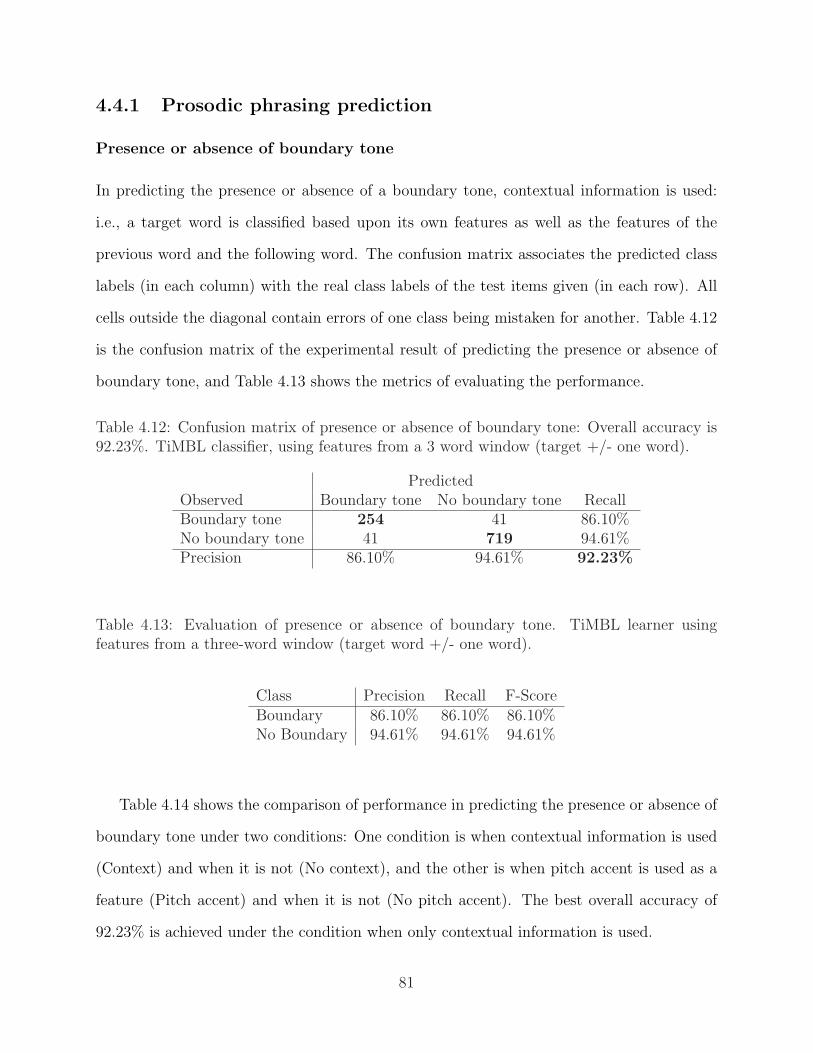
4.4.1 Prosodic phrasing prediction

Presence or absence of boundary tone

In predicting the presence or absence of a boundary tone, contextual information is used:

i.e., a target word is classified based upon its own features as well as the features of the

previous word and the following word. The confusion matrix associates the predicted class

labels (in each column) with the real class labels of the test items given (in each row). All

cells outside the diagonal contain errors of one class being mistaken for another. Table 4.12

is the confusion matrix of the experimental result of predicting the presence or absence of

boundary tone, and Table 4.13 shows the metrics of evaluating the performance.

Table 4.12: Confusion matrix of presence or absence of boundary tone: Overall accuracy is92.23%. TiMBL classifier, using features from a 3 word window (target +/- one word).

PredictedObserved Boundary tone No boundary tone RecallBoundary tone 254 41 86.10%No boundary tone 41 719 94.61%Precision 86.10% 94.61% 92.23%

Table 4.13: Evaluation of presence or absence of boundary tone. TiMBL learner usingfeatures from a three-word window (target word +/- one word).

Class Precision Recall F-ScoreBoundary 86.10% 86.10% 86.10%No Boundary 94.61% 94.61% 94.61%

Table 4.14 shows the comparison of performance in predicting the presence or absence of

boundary tone under two conditions: One condition is when contextual information is used

(Context) and when it is not (No context), and the other is when pitch accent is used as a

feature (Pitch accent) and when it is not (No pitch accent). The best overall accuracy of

92.23% is achieved under the condition when only contextual information is used.

81

Table 4.14: Overall comparison of performance in predicting the presence or absence ofboundary tone under two conditions of contextual information and prosodic information.

Features Overall accuracyNo context Pitch accent 92.01%No context No pitch accent 91.56%Context Pitch accent 92.22%Context No pitch accent 92.23%

Table 4.15 shows the effects of individual features in the prediction task of the presence

or absence of boundary tone. Information gained under the condition of no pitch accent, and

with contextual information from a three-word window. The features presented in the table

are confined to the features that are used under the condition of no contextual information.

The features are presented according to the order of features with higher gain ratio.

Strength of boundary tones

In predicting the strength of prosodic phrase boundary, no contextual information is used.

That is a target word is classified based upon its own features only. The result of predicting

the strength of prosodic phrase boundary of either intermediate phrase (ip) or intonation

phrase (IP) along with the location of boundary tone (BT) is shown in Table 4.16 and Table

4.17. These tables reveal that ip prediction is quite difficult to make. In correctly classifying

the intermediate phrase, only 27.88% precision and 45.31% recall rates were achieved. The

experiment reveals an aspect of prosodic boundary production and perception which is not

well understood.

Table 4.17 shows the evaluation of the boundary strength prediction: ip is Intermediate

Phrase and IP is Intonational Phrase. While predicting IP and no boundary tone is quite

accurate, predicting ip is quite difficult to make.

Table 4.18 shows the comparison of performance in predicting the strength of boundary

tone under two conditions of contextual and pitch accent information. The best overall

82

Table 4.15: Information gained under the condition of no pitch accent information, and withcontextual information from a three-word window. In the column ‘Context’, -1, 0, and +1are target word - one word, target word, and target word + one word, respectively. Thefeatures are presented in order with higher gain ratio.

Feature Context Information Gain Gain RatioNE bracket +1 0.1169 0.1442Named entity +1 0.1127 0.1411Number of phones +1 0.1155 0.1118Syntactic phrase ID + 1 0.1813 0.0915Sentence ID + 1 0.1305 0.0753Part of speech 0 0.1330 0.0746Syntactic phrase +1 0.2097 0.0668Part of speech +1 0.1108 0.0634NE bracket 0 0.0337 0.0614Syntactic phrase 0 0.1826 0.0603Grammatical role +1 0.1184 0.0579Sentence ID 0 0.0806 0.0536Part of speech 0 0.0795 0.0523Number of syllable +1 0.1431 0.0457Syntactic phrase ID 0 0.0697 0.0389Number of syllable 0 0.1154 0.0389Number of phones 0 0.0291 0.0376Location of primary stress -1 0.1379 0.0282Location of primary stress +1 0.1337 0.0273Location of primary stress 0 0.1337 0.0273NE bracket -1 0.0177 0.0212Named entity -1 0.0124 0.0150Syntactic phrase ID -1 0.0221 0.0109Named entity 0 0.0057 0.0106Syntactic phrase -1 0.0337 0.0105Number of phones -1 0.0082 0.0079Grammatical role -1 0.0117 0.0056Sentence ID -1 0.0086 0.0050Grammatical role 0 0.0066 0.0035Number of syllable -1 0.0086 0.0028

accuracy of 88.42% is achieved when pitch accent information is used, and no contextual

information is used. Unlike the prediction task of the presence or absence of prosodic bound-

ary, contextual information does not add to increasing the performance.

83

Table 4.16: Confusion matrix of strength of prosodic phrase boundary. Overall accuracy is88.06%. TiMBL learner using features from the target word only (no context).

PredictedObserved ip IP No BT Recallip 29 29 46 45.31%IP 14 164 11 80.00%No BT 21 12 730 92.76%Precision 27.88% 86.77% 95.68% 88.06%

Table 4.17: Evaluation of the strength of prosodic phrase boundary. TiMBL learner usingfeatures from the target word only (no context).

Class Recall Precision F-Scoreip 45.31% 27.88% 34.54%IP 80.00% 86.77% 88.71%No BT 92.76% 95.68% 94.19%

Table 4.18: Overall comparison of performance in predicting the strength of prosodic bound-ary under two conditions of contextual and pitch accent information.

Features Overall accuracyNo context Pitch accent 88.42%No context No pitch accent 88.06%Context Pitch accent 87.10%Context No pitch accent 87.58%

Types of boundary tone

Table 4.19 reveals that predicting the type of boundary tone, using the TiMBL learner, is

quite strongly affected by the frequency of each boundary type. For example, H-H% or

H-L%, which have low frequency of occurrence, are predicted at or below chance. Lack of

learning may be due to the nature of the corpus. H-H% is usually associated with canonical

yes-no questions, which are rarely attested in the corpus.

84

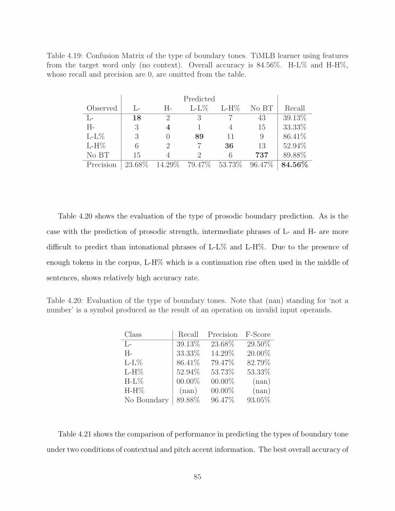
Table 4.19: Confusion Matrix of the type of boundary tones. TiMLB learner using featuresfrom the target word only (no context). Overall accuracy is 84.56%. H-L% and H-H%,whose recall and precision are 0, are omitted from the table.

PredictedObserved L- H- L-L% L-H% No BT RecallL- 18 2 3 7 43 39.13%H- 3 4 1 4 15 33.33%L-L% 3 0 89 11 9 86.41%L-H% 6 2 7 36 13 52.94%No BT 15 4 2 6 737 89.88%Precision 23.68% 14.29% 79.47% 53.73% 96.47% 84.56%

Table 4.20 shows the evaluation of the type of prosodic boundary prediction. As is the

case with the prediction of prosodic strength, intermediate phrases of L- and H- are more

difficult to predict than intonational phrases of L-L% and L-H%. Due to the presence of

enough tokens in the corpus, L-H% which is a continuation rise often used in the middle of

sentences, shows relatively high accuracy rate.

Table 4.20: Evaluation of the type of boundary tones. Note that (nan) standing for ‘not anumber’ is a symbol produced as the result of an operation on invalid input operands.

Class Recall Precision F-ScoreL- 39.13% 23.68% 29.50%H- 33.33% 14.29% 20.00%L-L% 86.41% 79.47% 82.79%L-H% 52.94% 53.73% 53.33%H-L% 00.00% 00.00% (nan)H-H% (nan) 00.00% (nan)No Boundary 89.88% 96.47% 93.05%

Table 4.21 shows the comparison of performance in predicting the types of boundary tone

under two conditions of contextual and pitch accent information. The best overall accuracy of

85

84.56% is achieved when no contextual information and no pitch accent information is used.

It seems that contextual information is only needed for predicting the prosodic boundary

location.

Table 4.21: Comparison of performance in predicting types of boundary tone under twoconditions of contextual and pitch accent information.

Features Overall accuracyNo context Pitch accent 82.85%No context No pitch accent 84.56%Context Pitch accent 81.99%Context No pitch accent 81.70%

4.4.2 Prosodic prominence prediction

Presence or absence of pitch accent

The same contextual information as in the task of prosody boundary prediction is used for

pitch accent prediction. That is, the features of the previous and the following words of the

target word are included in the input feature vector for predicting the presence or absence of

pitch accent. Table 4.22 is a confusion matrix for the prediction of the presence or absence

of pitch accent, and Table 4.23 shows the evaluation of this binary classification task.

Table 4.22: Confusion matrix of presence or absence of pitch accent. TiMBL learner observ-ing features from a three-word window (target word +/- one word).

PredictedObserved Pitch accent No pitch accent RecallPitch accent 507 48 86.22%No pitch accent 81 419 89.72%Precision 91.35% 83.80% 87.78%

Table 4.24 shows the comparison of performance in predicting the presence or absence of

pitch accent under two different conditions: when contextual information is used (Context)

86

Table 4.23: Evaluation of presence or absence of pitch accent. TiMBL learner observingfeatures from a three-word window (target word +/- one word).

Class Recall Precision F-ScorePitch accent 86.22% 91.35% 88.71%No pitch accent 89.72% 83.80% 86.65%

Table 4.24: Overall comparison of performance in predicting the presence or absence of pitchaccent under the conditions of contextual and boundary tone information

Features Overall accuracyNo context Boundary tone 85.72%No context No boundary tone 85.63%Context Boundary tone 87.67%Context No boundary tone 87.77%

and when it is not used (No context), when boundary tone is included as a feature (Boundary

tone) and when it is not included (No boundary tone). The best overall accuracy of 87.77%

is achieved when contextual information is used, and no information regarding boundary

tone used.

Table 4.25 shows the effects of individual features in the task of predicting the presence

or absence of pitch accent. Information gained under the condition of no prosodic boundary

information, and with contextual information from a three-word window. The features are

presented according to the order of features that have higher gain ratio.

Types of pitch accent

Different categories of tonal inventories are merged based on shared tonal targets. Thus, H*,

!H*, L* and No pitch accent are the categories I intend to predict.

The confusion matrix in Table 4.26 and the table showing the evaluation in Table 4.27

show that !H* is more likely to be classified as H* or No pitch accent (No PA). Given the

87

Table 4.25: Information gained under the condition of no prosodic boundary information,and with contextual information from a three-word window. In the column ‘Context’, -1, 0,and +1 are target word - one word, target word, and target word + one word, respectively.The features are presented in order with higher gain ratio.

Feature Context Information Gain Gain RatioSentence ID 0 0.1652 0.1098Syntactic phrase 0 0.3043 0.1005Number of syllable 0 0.2613 0.0880Number of phones 0 0.0473 0.0610NE bracket 0 0.0329 0.0598Named entity 0 0.0315 0.0587Syntactic phrase ID 0 0.0971 0.0542Number of syllable +1 0.3796 0.0449Part of speech 0 0.0622 0.0349NE bracket +1 0.0246 0.0304Syntactic phrase ID +1 0.0447 0.0225Named entity +1 0.0173 0.0217Syntactic phrase +1 0.0658 0.0209Number of phones +1 0.0172 0.0166Part of speech +1 0.0276 0.0158Syntactic phrase -1 0.0496 0.0155NE bracket -1 0.0108 0.0129Sentence ID +1 0.0189 0.0109Number of syllable -1 0.0309 0.0099Grammatical role +1 0.0198 0.0097Number of syllable +1 0.0279 0.0089Location of primary stress +1 0.0283 0.0057Location of primary stress 0 0.0283 0.0057Location of primary stress -1 0.0263 0.0053Grammatical role 0 0.0097 0.0052Named entity -1 0.0031 0.0038Syntactic phrase ID -1 0.0058 0.0029Number of phones -1 0.0025 0.0024Part of speech 0 0.0036 0.0024Sentence ID -1 0.0037 0.0021Grammatical role -1 0.0022 0.0010

scarcity of L* (259 or 0.2% in the whole corpus (i.e., both in the training and testing data

sets)), the learning algorithm performs quite poorly.

88

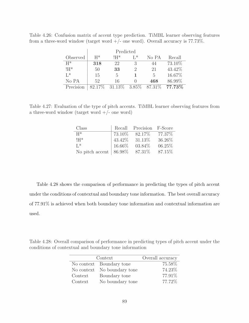
Table 4.26: Confusion matrix of accent type prediction. TiMBL learner observing featuresfrom a three-word window (target word +/- one word). Overall accuracy is 77.73%.

PredictedObserved H* !H* L* No PA RecallH* 318 22 3 44 73.10%!H* 50 33 2 21 43.42%L* 15 5 1 5 16.67%No PA 52 16 0 468 86.99%Precision 82.17% 31.13% 3.85% 87.31% 77.73%

Table 4.27: Evaluation of the type of pitch accents. TiMBL learner observing features froma three-word window (target word +/- one word)

Class Recall Precision F-ScoreH* 73.10% 82.17% 77.37%!H* 43.42% 31.13% 36.26%L* 16.66% 03.84% 06.25%No pitch accent 86.98% 87.31% 87.15%

Table 4.28 shows the comparison of performance in predicting the types of pitch accent

under the conditions of contextual and boundary tone information. The best overall accuracy

of 77.91% is achieved when both boundary tone information and contextual information are

used.

Table 4.28: Overall comparison of performance in predicting types of pitch accent under theconditions of contextual and boundary tone information

Context Overall accuracyNo context Boundary tone 75.58%No context No boundary tone 74.23%Context Boundary tone 77.91%Context No boundary tone 77.72%

89

4.5 Discussion and Conclusion

Even though predicting the tonal type of pitch accent and boundary tone decreases the per-

formance of overall accuracy, it should be noted that the results obtained in this experiment

are better than most earlier studies using a similar or the same corpus. Below in Table 4.29,

the example sentence “That year Thomas Maffy, now president of Massachusetts Bar Asso-

ciation, was Hennessy’s law clerk.” is aligned with observed prosodic labels and predicted

prosodic labels.

Table 4.29: The comparison of observed pitch accents and boundary tones with predictedpitch accents and boundary tones. The bold face indicates deviation of the predicted prosodicfeatures from the observed prosodic features. The method includes prosodic information inlearning, along with the above mentioned features.

Word Observed PredictedThat H* H*year !H* L-H% H* L-Thomas H* H*Maffy !H* L-L% H* L-L%nowpresident H* L- H* L-oftheMassachusettsbar H* H*association L-H% L-H%wasHennessy’s H* H*law H* H*clerk L-L% L-L%

The output shows both promising results and areas of difficulty. As is apparent, for some

words the learning algorithm fails to predict the desirable pitch accent type (H* instead of

!H*) or boundary type (L- instead of L-H%).12 On the other hand, my experimental result

12This is more complex to assess if we consider speaker variability in the production of pitch accents orboundary tones. For example, one speaker does not put pitch accent on the word ‘year ’, and/or produces

90

does not show over-generation of pitch accents or boundary tones on words where their

presence would be awkward or unreasonable. For example, it would be awkward, though

not impossible, to have a pitch accent on the preposition or determiner (e.g., of, the), or to

have a boundary tone between compound nouns (e.g., Bar Association).

One may wonder the relation between machine learning experimental results and inter-

speaker consistency, specifically, the apparently higher rate of prediction accuracy than that

of inter-speaker consistency. For example, in Chapter 2, it is reported that the rate of

consistency on the presence or absence of boundary tone is on average 89.71%. The accuracy

of predicting the presence or absence of boundary tone is 92%. Thus, it looks like the output

of machine learning is better than the human consensus. However, due to differences in the

calculation of prediction accuracy and inter-speaker consistency, it is not fair to compare the

two results without reservation. The inter-speaker consistency is calculated as a pair-wise

comparison on a pair of word and prosodic labels. For example, in calculating the rate of

consistency with regard to the presence or absence of prosodic boundary, two speakers are

judged to be consistent only if they both have, or do not have a prosodic boundary on a

given word. In this regard, the pair-wise consistency rate is a more stringent measure than

the overall prediction accuracy in the prediction task. The overall accuracy is calculated as

a harmonic measure of precision and recall, where mismatched prosodic labels for speakers

are taken into account as deletion or insertion errors.

Now, let’s consider the output of a different system. The example in (4.7) is an output

with two levels of phrasing prediction implemented in a Text-To-Speech (TTS) system called

Festival (Taylor & Black (1998)). Festival predicts the location of phrase boundaries using

only the POS features in a 6-word window; other linguistic features are not used. Here, two

levels of prosodic breaks are marked by B (small break) and BB (big break). Even though

L- on the word ‘year’, while another speaker produces ‘year’ with a !H* pitch accent and L-L% boundarytone. Nevertheless, the experimental result can be viewed as a ‘neutralized prosodic structure’ (Bachenko& Fitzpatrick 1990) which the machine learner learned and generalized from the similar instances withintraining data. Proper evaluation of the output deserves some form of perceptual experiment.

91

the Festival system is not trained on the same material, the comparison of the predicted

prosodic events in Table 4.29 and in (4.7) indicates that the approach of prosodic prediction

using various linguistic features outperforms the methods of prosodic prediction using only

part of speech information.

(4.7) Phrase break output produced by the Festival TTS system.

(That year Thomas Maffy) B

(now president of the Massachusetts bar association)B

(was Hennesy ’s law clerk) BB

In this experiment, I tried to predict pitch accent and boundary tone from linguistic

features including aspects of phonology, syntax, argument structure, and named entities.

The overall result suggests that prosodic structure can be predicted quite well using features

extracted from linguistic structures. Despite the encouraging result, two apparent problems

need to be tackled: (1) improved prediction of !H* and (2) improved discrimination of ip

and IP. These issues will be discussed in the following chapters.

92

Chapter 5

Integrative Models of ProsodyPrediction

5.1 Introduction

In Chapter 4, I have demonstrated that high performance of predicting pitch accents and

prosodic boundaries, especially with regard to the presence or absence of the prosodic events,

can be achieved using linguistic features extracted from components of phonology, syntax,

argument-structure and named entities. In this chapter, I test the performance of prosodic

structure prediction by using a combined acoustic and linguistic feature sets. It is reasonable

to expect better performance when the combined sets of acoustic and linguistic features are

used than when only one of the feature sets is used. It was observed in some earlier studies

that while acoustic features alone do not yield good performance, a combined set of acoustic

and linguistic features can boost the performance of predicting prosodic structure more than

either the acoustic features or the linguistic features alone (Sun 2002; Chen 2004; Brenier,

Cer, & Jurafsky 2005).

In what follows, I describe extraction of acoustic features based on F0, intensity, and

duration, and then I present the experimental results of predicting prosodic structure using

selected acoustic features and the combined acoustic and linguistic features. I show that,

unlike earlier studies that show improved performance of combined acoustic and linguistic

features, my experiment shows that the performance of combined acoustic and linguistic

features is no better than the performance of linguistic features.

93

5.2 Extraction of Acoustic Features

Prior research on the production and perception of prosody has shown that acoustic fea-

tures based on F0, intensity, and duration are good indicators of prosodic structure. These

acoustic features were extracted for each word in the corpus using the Praat speech analysis

package (Boersma & Weenink 2005),1 and the scientific computing package ‘scipy’2 in the

Python programming language,3 and the statistical analysis package R.4 The raw acous-

tic features are post-processed and normalized. In what follows, I describe extraction and

post-processing of the F0, intensity, and duration features.

5.2.1 F0

The features related to the F0 contour are extracted after post-processing and normalizing

raw F0 values from each word. Praat (Boersma & Weenink 2005) is used to extract raw F0

values from each speech file. Each speech file lasts a few minutes, and contains the recorded

speech of multiple utterances. Figure 5.1 illustrates the raw F0 contours of an utterance in

a speech file extracted from a female speaker. The word transcript is in (5.1). In the figure

and the word transcript, vertical bars demarcate intonational phrase boundaries. Twelve

instances of intonational phrasing are observed both in (5.1) and Figure 5.1.

(5.1) Wanted: | Chief Justice of the Massachusetts Supreme Court. | In April, | the

S.J.C.’s current leader, Edward Hennessy, | reaches the mandatory retirement age of

seventy, | and a successor is expected to be named in March. | It may be the most

important appointment | Governor Michael Dukakis makes | during the remainder of

his administration | and one of the toughest. | As WBUR’s Margo Melnicove reports,

| Hennessy will be a hard act to follow. |

1http://praat.org or http://www.fon.hum.uva.nl/praat/2http://scipy.org3http://python.org4http://www.r-project.org

94

Pitc

h (H

z)

Time (ms)0.5 2518

Example of Raw Pitch Contour

0

70

140

210

280

350

Figure 5.1: Raw pitch contour. Vertical bars demarcate Intonational Boundaries

The raw F0 contour is post-processed using linear interpolation and median filtering.5

Linear interpolation is applied to fill an unvoiced region of speech signal with the interpolated

F0 values. The linear interpolated F0 contour is further processed by median filtering.

Median filtering is a non-linear signal enhancement technique for smoothing signals while

preserving edges of the signals, that is, while perserving the begging and ending of the

utterance in each file. In the case of a one-dimensional signal, median filtering slides a

window of an odd number of elements (e.g., 11 pitch points in this experiment) along the

signal, replacing the center sample by the median of the samples in the window.6 Figure

5.2 illustrates the linear interpolated and median filtered F0 contour. In the figure, once

5See Kochanski (submitted) for problems of using simply maximum pitch value for accent decision.6http:://www.mathworks.com/

95

again, the vertical bars demarcate intonational phrase boundaries. The smoothed F0 contour

eliminates abrupt F0 values that are observable in the raw F0 contour.7P

itch

(Hz)

Time (ms)0.5 2518

Example of Postprocessed Pitch Contour

0

70

140

210

280

350

Figure 5.2: Post-processed pitch contour using linear interpolation and median filtering withthe window of 11 pitch. Again, as in Figure 5.1, the vertical bars demarcate IntonationalBoundary.

The post-processed pitch contour is further processed by z-transformation based on In-

tonational Phrase (IP), as in (5.2):

zIP =F0− µIP

σIP

(5.2)

7Shih (to appear, chapter 6) provides a detailed description of the segmental effects on F0 values. Thoughthe analysis of micro-prosodic effects is a challenging and interesting research topic, there are other sourcesof errors in the extracted F0 values, e.g., errors due to back ground noise. In this dissertation, only F0 valuesobtained after the interpolation and median filtering are used, so F0 values that changed too abruptedly areexpected to be filtered out.

96

The z-transformed F0 contour forms the basis for the following F0-related feature vectors:

Five IP-based normalized F0 values, and four polynomial coefficients.

First, five F0 values are extracted from equally distanced points in each word and used

as a set of normalized F0 features. The five IP-based normalized F0 values are denoted by

Norm-F0 1, Norm-F0 2, Norm-F0 3, Norm-F0 4, and Norm-F0 5, respectively.8

Second, polynomial coefficients are further extracted from the five equally spaced nor-

malized F0 values, and the coefficients are used as the other set of F0-related features.

Orthogonal polynomial decomposition is a technique that is useful in analyzing or describ-

ing contour shape (Levitt & Rabiner 1971), and is successfully used in Levitt & Rabiner

(1970) and Kochanski, Grabe, Coleman, & Rosner (2005) for prominence discrimination

tasks. However, it doesn’t appear that polynomial coefficients have been used as a set of

features in the previous studies on predicting prosodic structure conducted on the Boston

University Radio News corpus. A set of orthogonal polynomials approximate the F0 curve,

as described in Shih (to appear).9 If f0(ti) is the f0 value at time ti, then

f0(ti) = b0 + b1[ζ1(ti)] + b2[ζ2(ti)] + . . . + bk[ζk(ti)] + e(ti)

= f0(ti) + e(ti) (5.3)

where f0 is the measured contour; f0 is the fitted contour; ζk(ti) is a polynomial in ti of

degree k; b0, b1, . . . , bk are constants; and e(ti) is the deviation between F0 and f0 at ti (Shih

(to appear)).

I extract third-order polynomial coefficients, that is, four coefficients denoted by b0, b1,

b2, and b3, from the above-mentioned five IP-based normalized f0 values in each word. Some

of the coefficients have meaning: “The constant b0 represents the mean of the f0 contour,

8Figure 3.1 in Chapter 3 shows that one of the features is used in represented in the binary decision treein CART.

9The description of the orthogonal polynomial is based on Shih (to appear, chapter 3). See Levitt andRabiner 1970, Kochanski et al. 2005, Shih (to appear) for further information

97

and the coefficients b1 and b2 of the linear and quadratic polynomials indicate the slope and

the curvature of the f0 contour (Shih, to appear).”

In sum, the nine features (i.e., 5 normalized F0 values and 4 polynomial coefficients) are

extracted from the smoothed pitch contours and are used as feature vectors.

5.2.2 Duration

A number of duration-related features are extracted to be used as input feature vector. Four

numerical values related to the duration features and five categorical features are extracted,

as described below.

Duration measures are taken for each segment following segmentation and phone labeling

of the speech signal. Segmentation and labeling is automated by applying a forced alignment

of the speech signal to a phone string.10 Forced alignment refers to the process of generating

a phone alignment by making use of a known phoneme sequence. The phone string is taken

from the dictionary encoding of each word, and forced alignment is done using the HTK

Hidden Markov Model Toolkit (Young et al. 2005). The toolkit is a standard toolkit used

to build an automatic speech recognition (ASR) system. Simply speaking, Hidden Markov

Model (or HMM) is a collection of algorithms that seek to find hidden events such as phones

through observable events such as speech signals. Figure 5.3 shows the mean and standard

deviation of duration of each vowel, as obtained by using forced alignment.11

Using the phone labels obtained through the forced alignment procedure, in addition

to the word labels, I extract nine duration-related features. First, four numerical values

related to the duration features are: (1) the duration of the word, (2) the duration of the

10Two of the five speakers in the Boston University Radio Speech corpus are accompanied by phonelabeling, but not the remaining three speakers. To obtain phone labels, I applied forced alignment to thewhole corpus.

11Speech corpora are usually transcribed in plain text. The symbols in the x-axis in the figure are in ARPA-BET format, in which two ASCII characters represent a phoneme (with an exception of ‘axr’). The IPA(International Phonetic Alphabet) symbols that correspond to the ARPABET symbols in the figure are as fol-lows: oI (oy), aU (aw), 3~ (axr), aI (ay), l

"(el), o (ow), O(ao), A (aa), e (ey), æ (ae), n

"(en), i (iy), E (eh), u (uw),

2 (ah), U (uh), I (ih), @ (ax). For descriptions of ARPABET notation see, e.g., Young et al. 2005, or a lectureon ‘transcription’ in Speech Tools minicourse (http://www.isle.uiuc.edu/courses/htk/index.html).

98

oy aw axr ay el ow ao aa ey ae en iy eh uw ah uh ih ax

Vowel duration (ms)

vowel

dura

tion

(ms)

050

100

150

200

Figure 5.3: Mean and standard deviation of duration of each vowel in the Boston UniversityRadio Speech Corpus, as obtained through HMM-based forced alignment. The symbols inthe x-axis in the figure are in ARPABET format, in which two ASCII characters representa phoneme (with an exception of ‘axr’). The error bar at the center of each box plotindicates one standard deviation. The IPA (International Phonetic Alphabet) symbols thatcorrespond to the ARPABET symbols in the figure are as follows: oI (oy), aU (aw), 3~ (axr),aI (ay), l

"(el), o (ow), O(ao), A (aa), e (ey), æ (ae), n

"(en), i (iy), E (eh), u (uw), 2 (ah), U

(uh), I (ih), @ (ax).

word-initial segment, (3) the duration of the word-final nucleus, and (4) the duration of the

silent pause following the word, if there is any. Except for the word-duration and the silent

pause duration, all duration measurements are normalized.

Normalized duration measures are calculated based on observed segment durations, using

the normalization method of Wightman et al. (1992). The normalized duration of a segment

99

is measured as the number of standard deviation units (σ) from the mean duration (µ) of

that segment, as observed over the entire corpus. The phone-based normalization formula

is given in (5.4):

dki =

xki − µk

i

σk(5.4)

where xki is the observed duration of token xi, belonging to vowel phone class k.

Second, categorical features are also extracted in addition to the continuous numerical

features: (1) the word initial segment, (2) the segments that comprise the word final syllable

(i.e., onset, nucleus, and coda), and (3) categorical coding of the silent pause after the word

(‘sil’ for silent and ‘no-sil’ for no silent pause).

5.2.3 Intensity

Intensity-related features are extracted using phone-based intensity normalization. Intensity

is affected by the type of the segment. For example, vowels have higher intensity value than

consonants. To minimize the effects of segmental variation, phone-based intensity normal-

ization is applied on the corpus. The procedure is the same as the duration normalization,

as in (5.5):

Iki =

xki − µk

i

σk(5.5)

where xki is the observed intensity of token xi, belonging to vowel phone class k.

After the normalization, five normalized intensity values are extracted from equally

spaced points in each word. Also extracted from the normalized intensity within each word

are the third order polynomial coefficients calculated from the five normalized intensity

100

values. In total, nine intensity-related values are used as the input feature vector.

5.3 Integrative Predictive Model of Prosodic

Prominence

In this section, I first present experimental results on predicting the presence or absence

of pitch accent, and the presence or absence of prosodic boundary using acoustic features.

For the task of predicting the presence or absence of pitch accent, I show that the linear

combination of the polynomial coefficients can achieve quite high accuracy. For the task

of predicting the presence of absence of prosodic boundary, I will demonstrate that the

word-final syllable nucleus provides reliable cues. Then, I will present experimental results

on predicting finer distinctions of prosodic structure using both the acoustic and linguistic

features.

5.3.1 Prediction of the pitch accents using acoustic features

It has been often shown in the literature that acoustic features alone are not sufficient to

predict the location of pitch accents with an accuracy comparable to that obtained using

linguistic features or combined acoustic and linguistic features. The inadequacy of acoustic

features for prosody prediction is supported by recent results questioning the role of funda-

mental frequency in perceiving prosodic prominence (Kochanski et al. 2005). Kochanski et

al. illustrate that “contrary to textbooks and common assumptions, F0 plays a minor role in

distinguishing prominent syllables from the rest of the utterance (p. 1038).” They demon-

strate that patterns of loudness and duration are more important than F0 in perceiving

prosodic prominence.

I test the role of F0 features as expressed by polynomial coefficients. By using the

polynomial coefficients as input features to the MBL-based machine learning algorithm, I

101

obtained the following classification results in Table 5.1. Overall accuracy of 73.62% is

achieved in predicting the presence or absence of pitch accent.12

Table 5.1: Prediction of presence/absence of pitch accents using the third order polynomialcoefficient summary of the F0 trajectory in the target word. (Overall accuracy of 73.62%).

PredictedObserved Pitch accent No pitch accent Recall

Pitch accent 382 154 75%No pitch accent 124 394 71%

Precision 71% 76% 73.62%

The rate of overall accuracy is about 23% above the rate that one can expect from a

chance level performance. In this task, the 2nd and 3rd coefficients prove to be the most

useful. That is, the slope and curvature are useful in signaling the presence or absence of

pitch accent. The usefulness of the slope and curvature suggest that pitch accents should

be signaled by F0 movements, rather than pitch heights which are expressed by the first

polynomial coefficient.

It is not possible to compare directly my result of pitch accent prediction using the

polynomial coefficients with that of Kochanski et al. (2005). Nevertheless, my study shows

that features derived from the F0 contour contributes significantly to the determination of

pitch accent. The effect of the F0 information may result from a couple of differences in the

nature of corpus and experimental settings between mine and those of Kochanski (2005):

First, my corpus is rather consistent in speech style, wherea Konchanski et al. use six

different dialects of British English and different speech styles ranging from sentence reading

to spontaneous conversaion. The dialectal and stylistic characteristics may have obscured

statistical estimation.13 Second, in my study, the analytic domain is bounded to be words.

12Default parameters are used for the experiment. However, when the parameters are optimized, as Idiscuss below, then the performance of accurately predicting the presence or absence of pitch accent canreach as high as 75.6% with only the polynomial coefficients as input feature vector.

13The data used for the experiments in Kochanski et al. (2005) is available athttp://www.phon.ox.ac.uk/IViE/.

102

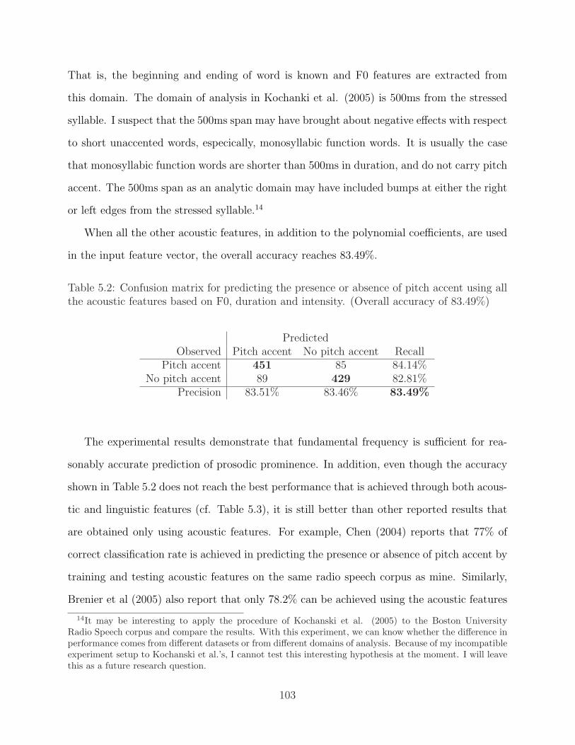
That is, the beginning and ending of word is known and F0 features are extracted from

this domain. The domain of analysis in Kochanki et al. (2005) is 500ms from the stressed

syllable. I suspect that the 500ms span may have brought about negative effects with respect

to short unaccented words, especically, monosyllabic function words. It is usually the case

that monosyllabic function words are shorter than 500ms in duration, and do not carry pitch

accent. The 500ms span as an analytic domain may have included bumps at either the right

or left edges from the stressed syllable.14

When all the other acoustic features, in addition to the polynomial coefficients, are used

in the input feature vector, the overall accuracy reaches 83.49%.

Table 5.2: Confusion matrix for predicting the presence or absence of pitch accent using allthe acoustic features based on F0, duration and intensity. (Overall accuracy of 83.49%)

PredictedObserved Pitch accent No pitch accent Recall

Pitch accent 451 85 84.14%No pitch accent 89 429 82.81%

Precision 83.51% 83.46% 83.49%

The experimental results demonstrate that fundamental frequency is sufficient for rea-

sonably accurate prediction of prosodic prominence. In addition, even though the accuracy

shown in Table 5.2 does not reach the best performance that is achieved through both acous-

tic and linguistic features (cf. Table 5.3), it is still better than other reported results that

are obtained only using acoustic features. For example, Chen (2004) reports that 77% of

correct classification rate is achieved in predicting the presence or absence of pitch accent by

training and testing acoustic features on the same radio speech corpus as mine. Similarly,

Brenier et al (2005) also report that only 78.2% can be achieved using the acoustic features

14It may be interesting to apply the procedure of Kochanski et al. (2005) to the Boston UniversityRadio Speech corpus and compare the results. With this experiment, we can know whether the difference inperformance comes from different datasets or from different domains of analysis. Because of my incompatibleexperiment setup to Kochanski et al.’s, I cannot test this interesting hypothesis at the moment. I will leavethis as a future research question.

103

they extracted. Tamburini & Cani (2005) report that 80.7% accuracy rate is achieved in the

same task, but at this time, on the TIMIT corpus.15

5.3.2 Prediction of pitch accents using integrative features

Now that the extracted acoustic features prove to be useful in predicting the presence or

absence of pitch accent, we may expect that we will further improve the performance of

the prosody prominence prediction by combining the acoustic features with the linguistic

features.

Before presenting experimental results, some discussion on the choice of parameters set

in the machine learning algorithms is in order. So far, I have limited the use of distance

and weighting parameters, as in (5.6), to the default setting as implemented in the TiMBL

learning algorithm, called ‘IB1-IG.’

∆(X,Y ) =∑

i

wiδ(xi, yi) (5.6)

An overlap metric is used for measuring the distance between new instance X and all

instances Y stored in memory. Information gain (IG) is used for the feature weighting. And

k = 1 in k-nn (k-nearest neighbor) is used to assign a class label to the new instance. But,

it is well known that the accuracy of a machine learning algorithm is affected by the setting

of parameters to a certain degree. Van den Bosch (2004) reports that the accuracy of a

machine learning algorithm can increase or decrease up to 30% when instead of its default

algorithmic parameter settings, one or more parameters are given a non-default value.It is

not practically feasible to test all possible combinations of parameter settings. Instead, I use

a software package ‘paramsearch’16 (van den Bosch 2004) to search for optimized parameter

15It is difficult to know how well the current approach will perform on the TIMIT corpus, and it is notpossible to compare directly the performance reported here and the one reported by Tamburini & Cani(2005). The difference in performace may arise from differet speech styles rather than different techinques.

16http://ilk.uvt.nl/~antalb/paramsearch/

104

settings, and report on the accuracy of predicting the prosodic structure obtained under the

optimized parameter settings.

The optimized parameter settings work as follows: the parameter search starts with

a small sample in the training set. The search progressively increases the training set,

while testing combinations of parameter settings on the increasing amounts of training data.

The process halts if one of the following conditions is met: (1) after the parameter setting

selection, only one setting is left. Or, (2) if several settings are still selected after the last

setting selection, then the parameter setting that meets one of the following sub-conditions

is selected: if default setting is present in the remaining settings, then the default setting is

returned. If not, a random selection is made among the selected settings, and the randomly

chosen setting is returned (van den Bosch 2004).

Presence or absence of pitch accent

For the binary classification task of predicting pitch accents using both the acoustic and

linguistic features, the best performance using the optimized parameter settings achieves an

accuracy rate of about 87.07%.17 This performance is almost as good as the performance

observed in Chapter 4 by using the linguistic features only, and is better than the performance

that can be achieved by using the acoustic features only. Figure 5.4 illustrates the overall

progress of exhaustive parameter search.18

Overall accuracy is in the y-axis, and combination of parameter settings and sample size,

as indicated by ‘step’, are on the x-axis. The overall accuracy is shown to fluctuate between

75% and 88%.

The accuracy rate of 87.07% is chosen to be the best from the range from 75% to 88%.

The best parameters that result in the best accuracy are chosen to be Jeffrey divergence for

17The description of available parameters in TiMBL is in Daelemans et al. (2003) and Hendrickx (2005).18Some methods of distance weighting are proposed to deal with large number of k in k-nn algorithm.

A couple of methods, including inverse distance weighting, are proposed that weight votes of instances inrelation to their distances to the new instance.

105

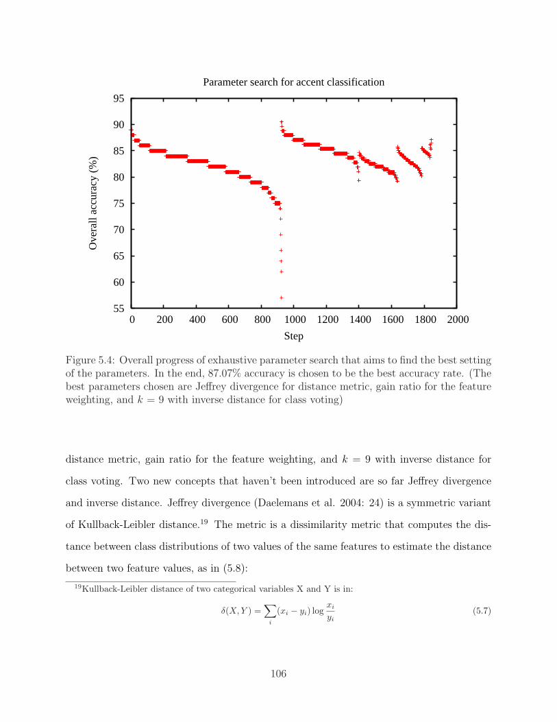
55

60

65

70

75

80

85

90

95

0 200 400 600 800 1000 1200 1400 1600 1800 2000

Ove

rall

accu

racy

(%

)

Step

Parameter search for accent classification

Figure 5.4: Overall progress of exhaustive parameter search that aims to find the best settingof the parameters. In the end, 87.07% accuracy is chosen to be the best accuracy rate. (Thebest parameters chosen are Jeffrey divergence for distance metric, gain ratio for the featureweighting, and k = 9 with inverse distance for class voting)

distance metric, gain ratio for the feature weighting, and k = 9 with inverse distance for

class voting. Two new concepts that haven’t been introduced are so far Jeffrey divergence

and inverse distance. Jeffrey divergence (Daelemans et al. 2004: 24) is a symmetric variant

of Kullback-Leibler distance.19 The metric is a dissimilarity metric that computes the dis-

tance between class distributions of two values of the same features to estimate the distance

between two feature values, as in (5.8):

19Kullback-Leibler distance of two categorical variables X and Y is in:

δ(X,Y ) =∑

i

(xi − yi) logxi

yi(5.7)

106

δ(v1, v2) =∑

i

P (Ci|vi) logPCi|vi)

m+ P ((Ci|vi) log

P (Ci|v2)

m(5.8)

where m is a normalization factor, as in (5.9):

m =P (Ci|v1) + P (Ci|v2)

2(5.9)

Some methods of distance weighting are proposed to deal with large number of k in

k-nn algorithm. The reason is because “when larger k values are used, the nearest neighbor

set can include, beside the similar and nearby instances, also a large group of less similar

instances. In such case majority voting may be less appropriate because the group of less

similar instances can override the classification of the nearby instances (Hendrickx 2005:

15).” Inverse distance weighting is one of the proposed distance weighting, in which the

inverse distance of a new instance to the nearest neighbor i is used, such that wi = 1/di.

It is not known whether the optimized parameter settings that are selected by the ‘param-

search’ after being evaluated on the training data will produce the same optimized perfor-

mance on unseen data. I conduct an experiment of predicting the presence or absence of

pitch accent on a test dataset containing 10% of the radio speech data, using parameters

trained on and obtained from the remaining 90% of the radio speech data. The 10% ran-

domly selected test data may or may not yield accuracy equal to the best accuracy obtained

through the parameter search algorithm. However, it is expected that the accuracy rate

obtained from the randomized test data is more or less in the vicinity of the optimized

accuracy rate. Table 5.3 is the confusion matrix that shows the results.

107

Table 5.3: Confusion Matrix on the task of predicting the presence or absence of pitch accentusing both linguistic and acoustic features under the best parameter setting obtained throughthe parameter search algorithm. The overall accuracy on independent test data (10% of theradio speech corpus) is 85.10%, which is slightly worse than the best performance reportedby the parameter search algorithm.

PredictedObserved Pitch accent No pitch accent Recall

Pitch accent 450 86 83.94%No pitch accent 71 447 86.29%

Precision 86.37% 83.86% 85.10%

Type of pitch accent

Table 5.4 shows the results of predicting types of pitch accent (H*, !H*, L*, and No Accent)

on the randomly chosen test data using both the acoustic and linguistic features under the

best parameter settings. The result in Table 5.4 does not meet our expectation that better

distinction will be made among the types of pitch accent using acoustic features together

with the linguistic features. Chapter 4 reports that 77.7% of overall accuracy can be achieved

using the features extracted from grammatical components. The reduction in accuracy in

Table 5.4 relative to the accuracy reported in Chapter 4 (Table 4.26) regarding !H* may

be due to either different parameter settings. For example, in the experiment reported in

Chapter 4, an overlap metric and k = 1 are used. In this experiment, the best parameters

are reported to be Jeffrey divergence for distance metric, no feature weighting and k = 35

with exponential decay distance for class voting. Exponential decay distance for class voting

is using the exponential decay function for weighting. It is the case that the larger the value

of k is, the more weight the more frequently occurring category gains. That is, the more

frequent H* tends to be over-predicted, compared to less frequent !H*.

108

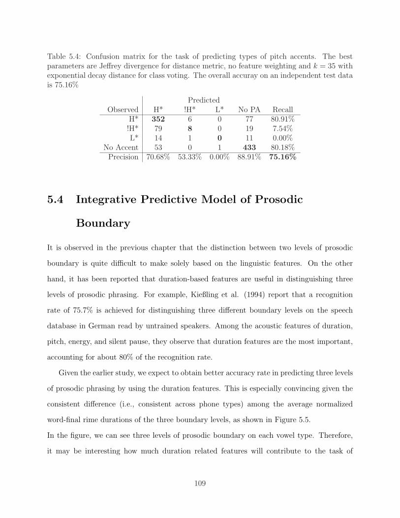
Table 5.4: Confusion matrix for the task of predicting types of pitch accents. The bestparameters are Jeffrey divergence for distance metric, no feature weighting and k = 35 withexponential decay distance for class voting. The overall accuray on an independent test datais 75.16%

PredictedObserved H* !H* L* No PA Recall

H* 352 6 0 77 80.91%!H* 79 8 0 19 7.54%L* 14 1 0 11 0.00%

No Accent 53 0 1 433 80.18%Precision 70.68% 53.33% 0.00% 88.91% 75.16%

5.4 Integrative Predictive Model of Prosodic

Boundary

It is observed in the previous chapter that the distinction between two levels of prosodic

boundary is quite difficult to make solely based on the linguistic features. On the other

hand, it has been reported that duration-based features are useful in distinguishing three

levels of prosodic phrasing. For example, Kießling et al. (1994) report that a recognition

rate of 75.7% is achieved for distinguishing three different boundary levels on the speech

database in German read by untrained speakers. Among the acoustic features of duration,

pitch, energy, and silent pause, they observe that duration features are the most important,

accounting for about 80% of the recognition rate.

Given the earlier study, we expect to obtain better accuracy rate in predicting three levels

of prosodic phrasing by using the duration features. This is especially convincing given the

consistent difference (i.e., consistent across phone types) among the average normalized

word-final rime durations of the three boundary levels, as shown in Figure 5.5.

In the figure, we can see three levels of prosodic boundary on each vowel type. Therefore,

it may be interesting how much duration related features will contribute to the task of

109

1

1 1

1

11

1

1

1

1

1

1 1

11

1

−0.

50.

00.

51.

01.

52.

0vowel duration and prosodic boundaries

Vowel

Nor

mal

ized

Dur

atio

n

2 2

2

2

2

2

22

2

2

2

2

2

2

2

2

3

3 3

33

3

3

33

3

3

3 3

33 3

aa ae ah ao aw ax ay eh el ey ih iy ow oy uh uw

Boundary

213

IPipWord

Figure 5.5: Average normalized rime duration of each phone type. Parameter is the level ofprosodic boundary (i.e., ip, IP, and Word). As in Figure 5.3, the symbols in the x-axis inthe figure are in ARPABET format.

predicting levels of prosodic boundary. Before presenting experiments using all the extracted

acoustic fetures, I illustrate the prediction of levels of prosodic phrasing using features related

to duration only. The duration-related features consist of the duration of the syllable nucleus,

stress location as calculated by subtracting the location of stress of a word from the number

of syllables in the word, the number of phones that occurs in the syllable onset, nucleus, and

coda position, respectively, and presence or absence of pitch accent. The data are divided

into 90% for training and 10% for testing. Applying the machine learning algorithm on

these features, we can achieve an overall accuracy of 80.45% in predicting levels of prosodic

boundary. Table 5.5 is the confusion matrix that shows the result of predicting levels of

110

prosodic boundary. The experimental result indicates that these duration-related features

extracted from the local pre-boundary syllable provide reliable cues for signaling levels of

prosodic boundary. Contrary to our hypothesis, however, it is still difficult to make a fine

distinction among the three boundary levels.

Table 5.5: Confusion matrix of strength of boundary tone using features related to durationonly. Overall accuracy of 80.45%

PredictedObserved ip IP No BT Recall

ip 25 31 60 21.55%IP 10 104 46 65.00%

No BT 24 35 719 92.41%Precision 42.37% 61.17% 87.15% 80.45%

Next, I address the question whether the prediction of prosodic boundary is more ac-

curately made if we use both acoustic and linguistic features. The set of acoustic features

has as its elements all features derived from F0, intensity, and duration, as presented in the

sections describing the extraction of acoustic features.

Presence or absence of boundary level

For the binary classification task of predicting the presence or absence of boundary tone by

using both the acoustic and linguistic features, the best performance using the optimized

parameter settings achieves an accuracy of 90.89%. The performance is slightly worse than

the performance observed using linguistic features only (about 92%). Figure 5.6 illustrates

the overall progress of exhaustive parameter search. The overall accuracy is in the range

between 77% and 91%.20

20Modified Value Difference Metric (DVDM, Daelemans et al. 2004:23) is a metric by which the distanceof the values of a feature is determined by “looking at co-occurrence of values with target classes,” as in:

δ(v1, v2) =∑

i

|P (Ci|v1)− P (Ci|v2)| (5.10)

111

55

60

65

70

75

80

85

90

95

0 500 1000 1500 2000 2500 3000

Ove

rall

accu

racy

(%

)

Step

Parameter search for IP boundary classification

Figure 5.6: Overall progress of exhaustive parameter search that results in the best setting.In the end, 90.89% is chosen to be the best accuracy. (The best parameters chosen areModified Value Difference Metric (MVDM) for distance metric, gain ratio for the featureweighting, and k = 25 with inverse distance for class voting.)

Table 5.6 is a confusion matrix that shows the results of predicting the presence or

absence of boundary tone using the best parameters on randomly selected test data (10% of

the radio speech corpus).

Table 5.6: Confusion matrix on the task of predicting prosodic boundary using both linguisticand acoustic features under the best parameter setting obtained through the parametersearch algorithm. The overall accuracy on test data is 90.60%.

PredictedBoundary tone No boundary tone Recall

Boundary tone 220 56 79.71%No boundary tone 43 735 94.47%

Precision 83.65% 92.92% 90.60%

112

Strength of boundary tone

Table 5.7 shows the confusion matrix for the experimental result of predicting levels of

prosodic boundary. Overall accuracy of 85.86% is achieved with the best parameters. The

best parameters consist of the modified value difference metric for the distance metric, no

feature weighting, and k = 15 with inverse distance weights for class voting.

Table 5.7: Confusion matrix on the task of predicting strength of prosodic boundary usingboth linguistic and acoustic features under the best parameter setting. The overall accuracyon test data is 85.86%.

PredictedObserved ip IP No BT Recall

ip 25 11 80 21.55%IP 12 122 26 76.25%

No BT 11 9 758 97.42%Precision 52.08% 85.91% 87.73% 85.86%

Types of boundary tone

Table 5.8 shows the confusion matrix of the experimental result of predicting tone type of

prosodic boundaries. The best parameters for the experiment are Jeffrey divergence for the

distance metric, information gain for the feature weighting, and k = 9 with exponential

decay for class voting. The overall accuracy of 83.42% is achieved for the prediction of types

of prosodic boundary. The performance is comparable to the one reported in Chapter 4

using only the linguistic features (cf. overall accuracy of 84.56%).

5.5 Discussion and Conclusion

This chapter described the extraction of acoustic features from F0, duration, and intensity. I

illustrated that the acoustic features are useful in predicting prosodic structure, and hypoth-

esized that integrating acoustic and linguistic features would result in improved performance

113

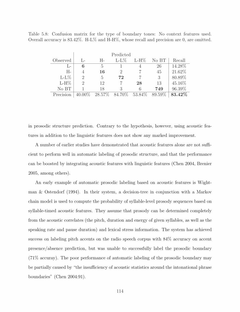
Table 5.8: Confusion matrix for the type of boundary tones: No context features used.Overall accuracy is 83.42%. H-L% and H-H%, whose recall and precision are 0, are omitted.

PredictedObserved L- H- L-L% L-H% No BT Recall

L- 6 5 1 4 26 14.28%H- 4 16 2 7 45 21.62%

L-L% 2 5 72 7 3 80.89%L-H% 2 12 7 28 13 45.16%

No BT 1 18 3 6 749 96.39%Precision 40.00% 28.57% 84.70% 53.84% 89.59% 83.42%

in prosodic structure prediction. Contrary to the hypothesis, however, using acoustic fea-

tures in addition to the linguistic features does not show any marked improvement.

A number of earlier studies have demonstrated that acoustic features alone are not suffi-

cient to perform well in automatic labeling of prosodic structure, and that the performance

can be boosted by integrating acoustic features with linguistic features (Chen 2004, Brenier

2005, among others).

An early example of automatic prosodic labeling based on acoustic features is Wight-

man & Ostendorf (1994). In their system, a decision-tree in conjunction with a Markov

chain model is used to compute the probability of syllable-level prosody sequences based on

syllable-timed acoustic features. They assume that prosody can be determined completely

from the acoustic correlates (the pitch, duration and energy of given syllables, as well as the

speaking rate and pause duration) and lexical stress information. The system has achieved

success on labeling pitch accents on the radio speech corpus with 84% accuracy on accent

presence/absence prediction, but was unable to successfully label the prosodic boundary

(71% accuray). The poor performance of automatic labeling of the prosodic boundary may

be partially caused by “the insufficiency of acoustic statistics around the intonational phrase

boundaries” (Chen 2004:91).

114

Chen (2004) presents an automatic prosodic labeling system to predict the presence or

absence of pitch accent and prosodic boundary. Chen (2004) reports that, when only acoustic

features are employed, 77% of correct classification accuracy is achieved in predicting the

presence or absence of pitch accent, and 68% of correct classification accuracy is achieved in

predicting the presence or absence of prosodic boundaries, which is worse than those reported

in Wightman & Ostendorf (1994). On the other hand, when both acoustic information and

syntactic information are used, the performance is boosted, that is, an accuracy of 84.7% for

pitch accent labeling and 93.1% for labeling of intonational phrase boundary.21 The syntactic

information is extracted from text using Charniak parsers, and is fed into an Artificial Neural

Network (ANN) to estimate the posterior probability of prosody given syntax. The acoustic

features are extracted and modeled as a Gaussian Mixture Model (GMM) for each allophone.

The experiments by Chen (2004) on the Boston Radio Speech corpus show that the model is

effective in learning the stochastic mapping from the acoustic and syntactic representation

of word strings to prosody labels.

In a similar vein, Brenier, Cer, & Jurafsky (2005) also report that overall accuracy rate

is 78.2% using acoustic features in predicting the presence or absence of pitch accent on

the Boston University Radio Speech corpus, and that accuracy using text-based features is

78.4%. When the acoustic features and text features are combined, the accuracy is 84.4%.

Based on the comparison of the results, they claim that “it was the combination of both

acoustic and text-based features that boosted performance for this task.”

Given all of these previously published results, why is it that the experimental results

reported here do not show any gain in combining the acoustic features with the textual

features, even though each set of features separately perform better, as shown in Table 5.9,

21Chen (2004) reports that the chance level for the presence or absence of boundary is 83%. The corpusin this dissertation is a subset of the same corpus as the one used in Chen (2004). But for my experiments,the chance level for the presence or absence of boundary is 72%. A possible source of difference is that whileI treated any levels of prosodic boundary to be the presence of prosodic boundary, Chen (2004) may havetreated only the intonational boundary (or break index 4) as the presence of prosodic boundary, in whichcase the baseline is higher than 72%.

115

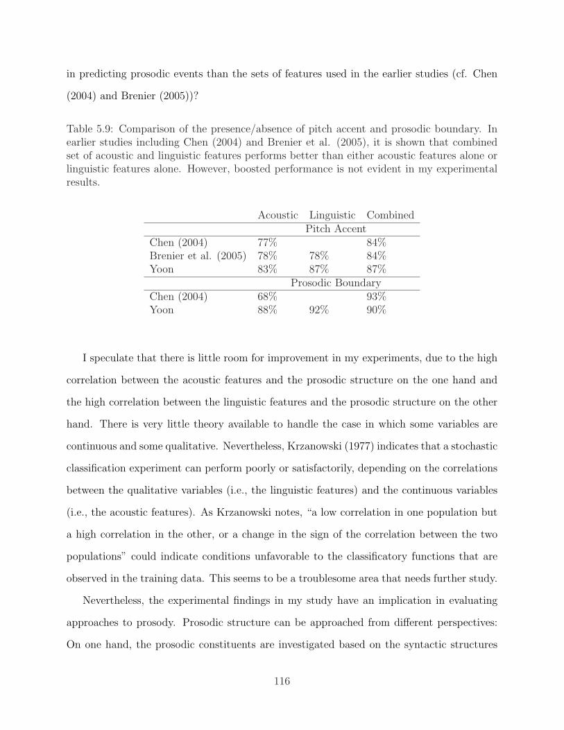
in predicting prosodic events than the sets of features used in the earlier studies (cf. Chen

(2004) and Brenier (2005))?

Table 5.9: Comparison of the presence/absence of pitch accent and prosodic boundary. Inearlier studies including Chen (2004) and Brenier et al. (2005), it is shown that combinedset of acoustic and linguistic features performs better than either acoustic features alone orlinguistic features alone. However, boosted performance is not evident in my experimentalresults.

Acoustic Linguistic CombinedPitch Accent

Chen (2004) 77% 84%Brenier et al. (2005) 78% 78% 84%Yoon 83% 87% 87%

Prosodic BoundaryChen (2004) 68% 93%Yoon 88% 92% 90%

I speculate that there is little room for improvement in my experiments, due to the high

correlation between the acoustic features and the prosodic structure on the one hand and

the high correlation between the linguistic features and the prosodic structure on the other

hand. There is very little theory available to handle the case in which some variables are

continuous and some qualitative. Nevertheless, Krzanowski (1977) indicates that a stochastic

classification experiment can perform poorly or satisfactorily, depending on the correlations

between the qualitative variables (i.e., the linguistic features) and the continuous variables

(i.e., the acoustic features). As Krzanowski notes, “a low correlation in one population but

a high correlation in the other, or a change in the sign of the correlation between the two

populations” could indicate conditions unfavorable to the classificatory functions that are

observed in the training data. This seems to be a troublesome area that needs further study.

Nevertheless, the experimental findings in my study have an implication in evaluating

approaches to prosody. Prosodic structure can be approached from different perspectives:

On one hand, the prosodic constituents are investigated based on the syntactic structures

116

of an utterance (Selkirk 1984, Nespor & Vogel 1986, cf. Steedman 2000). The syntax-

driven approach seeks to understand the mapping from syntactic structure to intonational

phrasing. On the other hand, the Autosegmental-Metrical theory of intonational phonol-

ogy (Pierrehumbert 1980, Beckman & Pierrehumbert 1986), on which the ToBI system is

based, investigates prosodic constituents on the basis of the perceived intonation pattern of

an utterance. The phonology/phonetics-driven perspective seeks to understand the phono-

logical structures that encode prosodic phrasing and accentuation, and how these structures

relate to other aspects of phonological structure (e.g., syllable, metrical structure). It is

also concerned with the acoustic correlates of intonational events, as a way of establishing

the empirical basis of investigation. In this chapter, I show that experimental results ob-

tained through the predictive model of prosodic structure, integrating features extracted

from grammatical components and the acoustic signal show that the linguistic features and

acoustic cues are highly correlated with each other. The results lead us to conclude that

the prosodic structure can be predicted on the basis of structural linguistic properties, and

detected on the basis of acoustic cues.

117

Chapter 6

Acoustic Correlates of ProsodicStructure

6.1 Introduction

I present two studies illustrating acoustic correlates of prosodic structure: one is concerned

with acoustic correlates of three levels of prosodic boundary and the other with acoustic

correlates of downstepped pitch accent. The experimental studies on predicting prosodic

structure reported in the previous chapters do not provide strong evidence for a distinction

between three levels of prosodic boundary or for the categorical status of downstepped pitch

accent. Relevant evidence from the study of acoustic correlates is shown to support these

less well understood and controversial components in the prosodic structure.

6.2 Acoustic Cues to Layered Prosodic Domains

This section investigates the phonetic encoding of prosodic structure through analysis of the

acoustic correlates of prosodic boundary and the interaction with phrase stress (i.e., pitch

accent) at three levels of prosodic structure: Word, ip, and IP. Prosodic structure encodes the

grouping of words into hierarchically layered prosodic constituents, including the prosodic

word, intermediate phrase (ip) and intonational phrase (IP) (Beckman & Pierrehumbert

1986; Ladd 1986, 1996; Keating, Cho, Fougeron, & Hsu 2003). Figure 6.1 illustrates an

example of the two levels of prosodic boundary. The two utterances in the figure are provided

by Beckman & Pierrehumbert 1986 as a canonical minimal pair that necessitates a level of

prosodic phrasing below intonational phrase, i.e., intermediate phrase. In Figure 6.1, the

118

F0 contours from the same strings “‘I’ means insert” are are represented, which differ from

each other regarding the prosodic realization of the subject “I.” The subject ‘I ’ in the second

utterance is marked with an intermediate phrase boundary, whereas the subject ‘I ’ in the

first utterance is not marked with any phrasal boundary.

H* H* L–L% H* L– H* L–L%

“I” means insert “I” means insert

0

400

100

200

300

Pitc

h (H

z)

Time (s)0 2.74603

Proposal of intermediate phrase boundary

Figure 6.1: An illustration of two levels of prosodic boundary of intermediate and intona-tional phrase. The F0 contours from the same word strings “‘I’ means insert” are presented,which differ from each other in the prosodic realization of the subject ‘I.’ The utterance “Imeans insert” can be realized with one prosodic phrasing unit, as on the left side, or it canbe realized with two prosodic phrasing units, as on the right side (Beckman & Pierrehumbert1986: 289).

Given the hierarchical organization, we expect to find non-elusive, audible acoustic cor-

relates of prosodic boundaries at each of these levels, but especially at the phrasal juncture

of ip and IP, to guide the listener in chunking the speech signal. Acoustic cues to prosodic

boundaries are observed in the lengthening of segments in the preboundary syllable (Lehiste,

Olive, & Streeter 1976; Selkirk 1984; Ladd & Campbell 1991; Wightman, Shattuck-Hufnagel,

Ostendorf, & Price 1992, Berkovits 1993), especially in the lengthening of the preboundary

rime, with greater effects of lengthening at successively higher levels of prosodic domains

(Wightman et al. 1992). A second dimension of prosodic structure is the encoding of promi-

nence, which also gives rise to lengthening effects in the prominent syllable (Turk & Sawush

119

1997; Turk & White 1999; Cambier-Langeveld & Turk 1999).

Given two distinct sources of lengthening, the question arises whether lengthening on

its own can serve as a cue to either prosodic context. An additional question is whether

the acoustic correlates of prominence and juncture are differentiated for syllables that are

doubly marked (i.e., both accented and phrase-final). I investigate the phonetic encoding of

prosodic structure through a study of duration as an acoustic correlate of prosodic boundary

and the interaction between boundary and accent effects at three levels of prosodic structure:

Word, ip, and IP. Guided by earlier evidence that boundary cues are local (Wightman et

al. 1992), evidence for acoustic effects of prosodic boundary is considered in measures of

duration local to the domain-final rime.

6.2.1 Acoustic cues for prosodic boundary

Silent pause and pre-boundary lengthening are known to be acoustic correlates of prosodic

boundary in English. While silent pause is neither a necessary nor sufficient boundary cue,

the potential value of lengthening as a boundary cue is questionable given that there are two

distinct sources of lengthening: boundary and accent. The possibly confounding interaction

between boundary and accent lengthening motivates the current study.

Silent pause:

There is a strong correlation between the presence of a pause and the perception of a prosodic

boundary; however, the perception of a prosodic boundary does not depend on the occurrence

of silent pause. Figure 6.2 is taken from the Boston University Radio Speech corpus, and

illustrates low-toned ip (L-) and low-toned IP (L-L%). In the figure, two instances of L-

observed on words “Hennessy” and “act” are not necessarily followed by any audible silent

pause.

Table 6.1 presents the correlation between the presence or absence of silent pause and

the presence or absence of phrasal boundary (either ip or IP) in the the Boston University

120

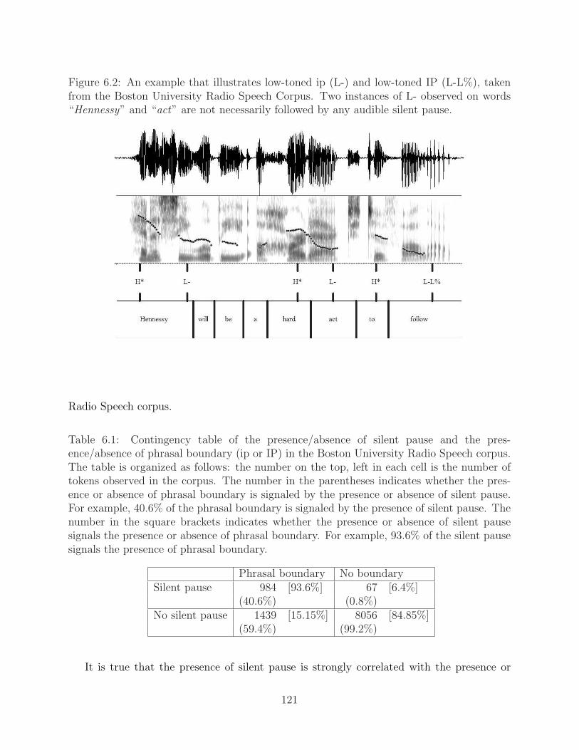
Figure 6.2: An example that illustrates low-toned ip (L-) and low-toned IP (L-L%), takenfrom the Boston University Radio Speech Corpus. Two instances of L- observed on words“Hennessy” and “act” are not necessarily followed by any audible silent pause.

Radio Speech corpus.

Table 6.1: Contingency table of the presence/absence of silent pause and the pres-ence/absence of phrasal boundary (ip or IP) in the Boston University Radio Speech corpus.The table is organized as follows: the number on the top, left in each cell is the number oftokens observed in the corpus. The number in the parentheses indicates whether the pres-ence or absence of phrasal boundary is signaled by the presence or absence of silent pause.For example, 40.6% of the phrasal boundary is signaled by the presence of silent pause. Thenumber in the square brackets indicates whether the presence or absence of silent pausesignals the presence or absence of phrasal boundary. For example, 93.6% of the silent pausesignals the presence of phrasal boundary.

Phrasal boundary No boundarySilent pause 984 [93.6%] 67 [6.4%]

(40.6%) (0.8%)No silent pause 1439 [15.15%] 8056 [84.85%]

(59.4%) (99.2%)

It is true that the presence of silent pause is strongly correlated with the presence or

121

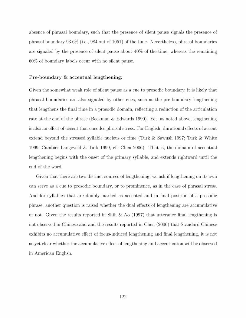
absence of phrasal boundary, such that the presence of silent pause signals the presence of

phrasal boundary 93.6% (i.e., 984 out of 1051) of the time. Nevertheless, phrasal boundaries

are signaled by the presence of silent pause about 40% of the time, whereas the remaining

60% of boundary labels occur with no silent pause.

Pre-boundary & accentual lengthening:

Given the somewhat weak role of silent pause as a cue to prosodic boundary, it is likely that

phrasal boundaries are also signaled by other cues, such as the pre-boundary lengthening

that lengthens the final rime in a prosodic domain, reflecting a reduction of the articulation

rate at the end of the phrase (Beckman & Edwards 1990). Yet, as noted above, lengthening

is also an effect of accent that encodes phrasal stress. For English, durational effects of accent

extend beyond the stressed syllable nucleus or rime (Turk & Sawush 1997; Turk & White

1999; Cambier-Langeveld & Turk 1999, cf. Chen 2006). That is, the domain of accentual

lengthening begins with the onset of the primary syllable, and extends rightward until the

end of the word.

Given that there are two distinct sources of lengthening, we ask if lengthening on its own

can serve as a cue to prosodic boundary, or to prominence, as in the case of phrasal stress.

And for syllables that are doubly-marked as accented and in final position of a prosodic

phrase, another question is raised whether the dual effects of lengthening are accumulative

or not. Given the results reported in Shih & Ao (1997) that utterance final lengthening is

not observed in Chinese and and the results reported in Chen (2006) that Standard Chinese

exhibits no accumulative effect of focus-induced lengthening and final lengthening, it is not

as yet clear whether the accumulative effect of lengthening and accentuation will be observed

in American English.

122

6.2.2 Methods

Evidence for acoustic effects of prosodic boundary is shown in measures of duration local

to the domain-final syllable rime. Duration measures are taken for each segment following

segmentation and phone labeling of the speech signal. As discussed in the previous chapter,

segmentation and labeling is automated by doing a forced alignment of the speech signal to

a phone string. The phone string is taken from the dictionary encoding of each word, and

forced alignment is done using the HTK Hidden Markov Model Toolkit (Young et al. 2005).

To reiterate, normalized duration measure is calculated based on observed segment durations,

using the normalized method of Wightman et al. (1992). The normalized duration of a

segment is measured as the number of standard deviation units (σ) from the mean duration

(µ) of that segment, as observed over the entire corpus. The phone-based normalization

formula is given in (6.1) (repeated from (5.4)):

dki =

xki − µk

i

σk(6.1)

where xki is the observed duration of token xi, belonging to vowel phone class k.

Table 6.2 shows the number of tokens of each vowel type in the corpus, and the distri-

bution of vowels under the condition of pitch accent and phrasal boundary of either ip or

IP. In the table, A stands for pitch accent, and B stands for phrasal boundary of either

intermediate or intonational phrases. For example, (No A, No B) indicates that the vowel

is not associated with any accent or boundary.

Duration measures are taken from the nucleus segment(s) of syllables in word-final posi-

tion in three prosodic contexts, as illustrated in Figure 6.3: (1) phrase-medial position, (2)

intermediate phrase-final position, and (3) intonational phrase-final position.

123

Table 6.2: Frequency table of vowels occurring at word-final syllable. In the table, A standsfor pitch accent, and B stands for phrasal boundary of either intermediate or intonationalphrases. The symbols are in ARPABET and the corresponding IPA symbols in parentheses.column.

Total (No A, No B) (A,No B) (No A, B) (A, B)

aa (A) 353 177 64 5 107ae (æ) 702 403 102 32 165ah (2) 756 443 91 20 202ao (O) 543 202 117 61 163aw (aU) 132 47 21 15 49ax (@) 1648 173 628 162 685axr (3~) 10 10ay (aI) 343 128 78 13 124eh (E) 536 175 130 50 181el (l

") 47 7 11 29

en (n") 15 4 2 9

ey (e) 892 450 137 41 264ih (I) 1671 800 265 74 532iy (i) 1742 883 315 57 487ow (o) 377 57 119 35 166oy (oI) 42 5 25 3 9uh (U) 84 47 10 4 23uw (u) 653 435 68 20 130Total 10546 4432 (42.0%) 2195 (20.8%) 594 (5.6%) 3325 (31.5%)

6.2.3 Results

Lexical stress (i.e., word-level prominence) may also influence segment duration, so separate

analyses are performed based on the location of lexical stress relative to the target word-final

syllable, as shown in the schematic diagram in Figure 6.4.

As the present study is concerned with the interaction of final lengthening with accentual

lengthening, the data are restricted to those syllables that are final in a prosodic domain,

and in the domain of accentual lengthening (i.e., in the accented stress foot). Final syllables

in words where lexical stress falls on a syllable that precedes the penultimate syllable are

124

Figure 6.3: Measurement domain for normalized duration. Measurements are taken fromthe syllable nucleus, as indicated by the circled x, in word-final position under the contextof phrase-medial, intermediate phrase-final, and intonational phrase-final positions.

Figure 6.4: Schematic diagram of the two locations of word-level stress, as indicated by " infront of the stressed syllable σ, for words in the present study. Duration measurements aretaken from the word-final syllable at the prosodic boundary (Word, ip, or IP).

(a) (b)[. . .σ σ "σ ]BND [. . .σ "σ σ ]BND

not eligible for accentual lengthening, based on the findings of Turk & Sawush (1997). Thus

the present study is limited to analysis of duration from word-final syllables in words with

lexical stress on the final or penultimate syllables.

Prosodic effects on normalized duration measures are tested using ANOVA with the

independent factors of Boundary (Word, ip, IP) and Accent (Accented, Unaccented), and

with separate ANOVAs for the two conditions of lexical stress location shown in Figure 6.4.

Lexical stress on the pre-boundary syllable:

The results of duration measures for the condition with lexical stress on the final syllable

(Figure 6.4a) are presented first. Table 6.3 shows the number of tokens available for analysis

under the two conditions of pitch accent and three boundary levels, from words which stress

125

Table 6.3: Frequency table of vowels occurring at word-final syllable under the condition ofthe location of lexical stress(penult stress and final stress)

Boundary No. of tokens No. of tokens(Final stress) (Penult stress)

ip 283 256Pitch accent IP 347 364

Word 1424 1512ip 136 53

No pitch accent IP 272 171Word 3864 288Total 6424 2644

falls on the final syllable (the 3rd column), and from words which stress falls on the penult

(the last column).

Figure 6.5 shows the effects of prosodic boundary on final nucleus duration. In both

accented and unaccented contexts, the normalized duration increases with the level of

the prosodic boundary in the hierarchy (Word < ip < IP) (Accented: F (2, 2051)=341.8,

p<0.001; Unaccented: F (2, 4267)=345.1, p<0.001). This demonstrates a three-way distinc-

tion of prosodic boundaries.

Figure 6.6 shows the effect of pitch accent on the nucleus duration. The normalized dura-

tion is significantly longer when the nucleus is accented than when the nucleus is unaccented,

for all levels of prosodic boundary (Word: F (1, 5286)=449.5, p<0.001; ip: F (1, 417)=13.2,

p<0.001; IP: F (1, 617)=58.5, p<0.001). This finding demonstrates an accumulative effect

of lengthening due to accent and prosodic boundary.1

1Many studies by van Santen (e.g., van Santen 1992, 1994) on duration modeling in English show thatsegmental duration is not adequately modeled by using either additive model or multiplicative model. Heproposes a sums-of-products model of segmental duration, in which various factors such as segmental identityand stress contribute both additively and multiplicatively to determining the duration of a segment. Shih(p.c.) points out that the segmental duration of Mandarin Chinese can be adequately modeled using amultiplicative model.

126

Figure 6.5: Effect of prosodic boundary on final nucleus duration (final stress). The asterisk *indicates that the difference between the two adjacent mean values on the plot is statisticallysignificant.

Lexical stress on the penultimate syllable:

Next, results of duration nucleus measures are presented for the conditions in Figure 6.4b,

where lexical stress occurs on the penultimate syllable. Bear in mind that the duration mea-

surements are taken from the final nucleus, and not from the penultimate stressed syllables.

See Table 6.3 (the last column) for the number of words with stress falls on the penultimate

syllable.

Figure 6.7 illustrates the effect of prosodic boundary on final nucleus duration. The

normalized duration of the final post-stress syllable nuclei in Figure 6.7 are shorter than the

normalized durations from the final stressed syllable in Figure 6.5. Nevertheless, Figure 6.7

shows the same three-way contrast in duration according to the level of prosodic boundary as

127

Figure 6.6: Effect of pitch accent on final nucleus duration (final stress).

in Figure 6.5 (Accented: F (2, 2129)=121.6, p<0.001; Unaccented; F (2, 509)=27.8, p<0.001).

Figure 6.8 illustrates the effect of accent-induced lengthening on the final nucleus dura-

tion. Based on the work by Turk & her colleagues, it is hypothesized that accent would cause

lengthening of the post-accented syllable in each of the prosodic boundary conditions. The

results show that this hypothesis is confirmed only for final post-accented syllables in IP-

final position, but not at the two lower levels of prosodic boundary (Word: F (1, 1798)=1.5,

p>0.2; ip: F (1, 307)=0.37, p>0.5; IP: F (1, 533)=8.1, p<0.005).

In summary, there are significant and increasing effects of final lengthening for the nucleus

in the final syllable of the Word, ip, and IP, supporting a 3-way distinction for word-final

syllables according to the prosodic phrase context. As expected, pitch accent also induces

128

Figure 6.7: Effect of prosodic boundary on final nucleus duration (penult stress).

lengthening of the accented syllable nucleus, but accented lengthening effects on the post-

accented, word-final syllable are observed only for syllables that are final in the IP, and not

in final position of the ip or Word. The discrepancy between the findings reported in this

section and those of Turk & her colleagues may be due to differences in the focus conditions

for the accents. In the radio speech materials, most pitch accents mark broad focus (new

information), with relatively few emphasis or contrastive focal accents. In the materials

constructed by Turk & her colleagues (Turk & Sawush 1997; Turk & White 1999; Cambier-

Langeveld & Turk 1999), accents mark contrastive focus. Contrastive focal accents are

observed to have larger pitch movements, and may also exhibit stronger effects of accentual

lengthening.

129

Figure 6.8: Effect of accent-induced lengthening on final nucleus duration (penult stress).

6.2.4 Conclusion

In conclusion, we find strong evidence for lengthening effects conditioned by prosodic bound-

aries and by phrasal prominence. The boundary lengthening effects distinguish three levels

of prosodic domains, and thus support a theory of prosodic structure that discriminates

between levels of prosody phrasing, such as ip and IP, in addition to the prosodic word. We

also demonstrate that lengthening effects due to accent and boundary are fully accumula-

tive for final accented syllables, and partially accumulative for final post-accented syllables.

Finally, our study provides evidence for local effects of prosodic domains in the syllable at

the right edge.

130

6.3 Downstepped Pitch Accents

6.3.1 Introduction

Downstepped pitch accent is the other problematic category for which the prediction exper-

iments in the previous chapters have performed poorly. Evidence is presented from acoustic

analysis and a (controlled) machine learning experiment for a categorical distinction be-

tween downstepped and non-downstepped high-toned pitch accents (H* vs. !H*). The

present study offers an explanation for the contradictory findings from prior acoustic studies

of downstep (Liberman & Pierrehumbert 1984 vs. Dainora 2001a,b), which call into question

the status of the downstepped accent in American English as a legitimate prosodic category.

Dainora (2001ab) suggests that there is a single phonological High tone that can be used in

the specification of pitch accent melody, and “downstepped” pitch accents are illusory, being

no more than a subset of variants taken from the normal distribution of H* peak values. On

the contrary, I show that the experimental findings from the same speech corpus as the one

used by Dainora does not support the null hypothesis, i.e., that downstepped !H* is not a

distinct prosodic category from H*.

Dowstepped high tones are high tones that occur in a compressed pitch range, as in Figure

6.9, either because of a bitonal pitch accent (Pierrehumbert 1980; Beckman & Pierrehumbert

1986), or because of a register feature on a high tone (Ladd 1983, 1996; Gussenhoven 1983;

Grice 1995; Truckenbrodt 1998; Beckman & Ayers 1997; Beckman 1996). Downstep has

been claimed to be a central part of the theory of intonation, providing a crucial argument

against multiple levels of tonal representation and in favor of more restrictive two-level tonal

representations using only high (H) and Low (L) tones (Pierrehumbert 1980, 2000; Grice

1995, 2003; Grabe 1998; Terken & Hermes 2000, Shih & Sproat 2001; Gussenhoven 2002,

among others).

As such, aspects of downstep have been studied cross-linguistically. Detailed empirical

studies of downstep and related effects of tonal scaling are reported in Liberman & Pierre-

131

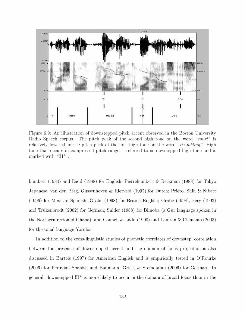
Figure 6.9: An illustration of downstepped pitch accent observed in the Boston UniversityRadio Speech corpus. The pitch peak of the second high tone on the word “court” isrelatively lower than the pitch peak of the first high tone on the word “crumbling.” Hightone that occurs in compressed pitch range is referred to as dowstepped high tone and ismarked with “!H*”.

humbert (1984) and Ladd (1988) for English; Pierrehumbert & Beckman (1988) for Tokyo

Japanese; van den Berg, Gussenhoven & Rietveld (1992) for Dutch; Prieto, Shih & Nibert

(1996) for Mexican Spanish; Grabe (1998) for British English; Grabe (1998), Fery (1993)

and Trukenbrodt (2002) for German; Snider (1988) for Bimoba (a Gur language spoken in

the Northern region of Ghana); and Connell & Ladd (1990) and Laniran & Clements (2003)

for the tonal language Yoruba.

In addition to the cross-linguistic studies of phonetic correlates of downstep, correlation

between the presence of downstepped accent and the domain of focus projection is also

discussed in Bartels (1997) for American English and is empirically tested in O’Rourke

(2006) for Peruvian Spanish and Baumann, Grice, & Steindamm (2006) for German. In

general, downstepped !H* is more likely to occur in the domain of broad focus than in the

132

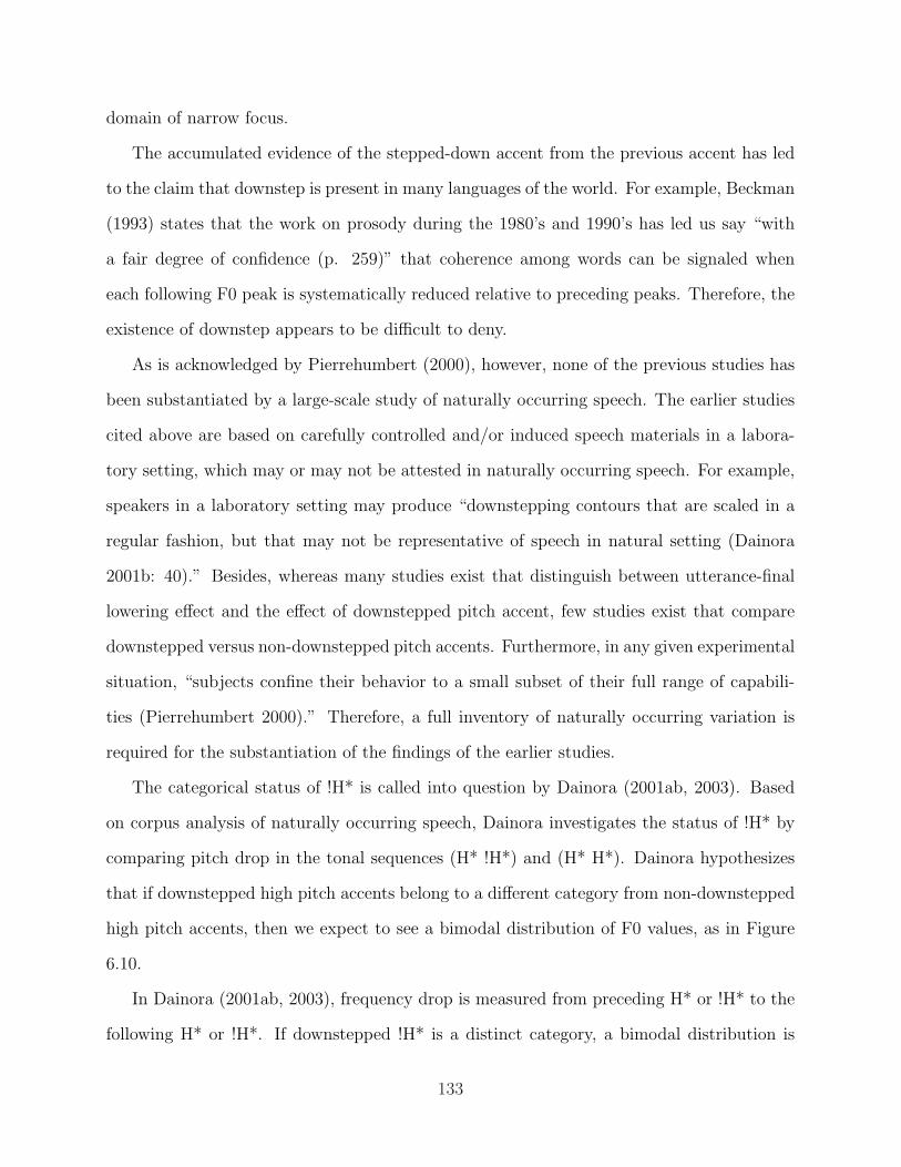
domain of narrow focus.

The accumulated evidence of the stepped-down accent from the previous accent has led

to the claim that downstep is present in many languages of the world. For example, Beckman

(1993) states that the work on prosody during the 1980’s and 1990’s has led us say “with

a fair degree of confidence (p. 259)” that coherence among words can be signaled when

each following F0 peak is systematically reduced relative to preceding peaks. Therefore, the

existence of downstep appears to be difficult to deny.

As is acknowledged by Pierrehumbert (2000), however, none of the previous studies has

been substantiated by a large-scale study of naturally occurring speech. The earlier studies

cited above are based on carefully controlled and/or induced speech materials in a labora-

tory setting, which may or may not be attested in naturally occurring speech. For example,

speakers in a laboratory setting may produce “downstepping contours that are scaled in a

regular fashion, but that may not be representative of speech in natural setting (Dainora

2001b: 40).” Besides, whereas many studies exist that distinguish between utterance-final

lowering effect and the effect of downstepped pitch accent, few studies exist that compare

downstepped versus non-downstepped pitch accents. Furthermore, in any given experimental

situation, “subjects confine their behavior to a small subset of their full range of capabili-

ties (Pierrehumbert 2000).” Therefore, a full inventory of naturally occurring variation is

required for the substantiation of the findings of the earlier studies.

The categorical status of !H* is called into question by Dainora (2001ab, 2003). Based

on corpus analysis of naturally occurring speech, Dainora investigates the status of !H* by

comparing pitch drop in the tonal sequences (H* !H*) and (H* H*). Dainora hypothesizes

that if downstepped high pitch accents belong to a different category from non-downstepped

high pitch accents, then we expect to see a bimodal distribution of F0 values, as in Figure

6.10.

In Dainora (2001ab, 2003), frequency drop is measured from preceding H* or !H* to the

following H* or !H*. If downstepped !H* is a distinct category, a bimodal distribution is

133

EH*E!H*

Hypothesized Bi-modal Distribution

Figure 6.10: Hypothetical bimodal distribution. If downstepped high pitch accents belongto a different category from non-downstepped high pitch accents, then it is expected that abimodal distribution will be revealed out of F0 values, such that the expected value of H*(EH∗) is higher than the expected value of !H* (E!H∗).

expected to be revealed, as in Figure 6.10. Unlike the expectation, however, the measurement

of frequency drop reveals a uni-modal distribution, as shown in Figure 6.11. Based on the

uni-modal distribution, Dainora argues that downstepped !H* is not a distinctive prosodic

category, at least in American English.

She claims that there is a single phonological high tone that can be used in specifying

pitch accent melody, and downstepped accent is illusory and is no more than a subset of

variants taken from the normal distribution of H* peak values, as in Figure 6.11. That

is, she maintains that the difference between downstepped and nondownstepped accents is

“a superficial one that does not belong in a model of intonation in English (p. 66),” and

“speakers produce tones that fluctuate around a given target point. The amount that the

frequency of a tone falls between the initial tone and the following tone is a random amount

134

Histogram of Pitch Drop

Frequency Difference (Hz)

Num

ber

of O

bser

vatio

ns

−150 −100 −50 0 50 100 150

020

4060

8010

012

0

Figure 6.11: The pitch drop measure defines a uni-modal distribution, where H* and !H*belong to opposite ends of a single distribution in the F0 dimension. The figure is obtainedthrough the same measurement as taken by Dainora and the result replicates Dainora’sresult.

(pp. 66-67).” The failure to substantiate the status of downstepped accent in American

English as a legitimate prosodic category raises a wholesale question to the central role of

downstep in the standard autosegmental-based theory of intonation (Grice 2003).

6.3.2 Categorical status of !H*

The present study offers an alternative approach to test the hypothesis whether or not

downstepped pitch accents are categorically different from non-downstepped pitch accents.

135

Categorical perception means that a change in some variable along a continuum is perceived

not as a continuum, but as instances of discrete categories.2 Given the different categorical

status between H* and !H*, stimuli from different categories such as downstepped !H* and

non-downstepped H* should be perceived differently, no matter how close the two categories

are on the continuum. Traditionally, a test for categorical perception consists of two compo-

nents: a labeling test and a discrimination test. In the study at hand, the labeling test is done

by transcribers who have labeled the ToBI labels including H* and !H* on the Boston Radio

Speech corpus. It needs to be tested whether any measures taken from the two categories

form different distributions. A bimodal distribution of two different categories reinforces our

perceptual basis for the discreteness of different categories, but in theory, measures taken

from two categories may not necessarily reveal bimodal distribution. A discrimination test

is performed by setting up a controlled machine learning experiment that is designed to

classify H* and !H*.

I argue that my results do not confirm the hypothesis that !H* in American English is

not a legitimate prosodic category. I apply an alternative method of analysis to the same

set of data from the Boston University Radio Speech corpus as is used by Dainora (2001ab,

2003). I argue that Dainora’s study has failed to consider the effects of peak height on the

pitch measure. Specifically, the F0 peak of the first H* in the sequence might condition the

magnitude of the pitch drop to a following pitch peak. In an alternative analysis developed

here, the peak of the second pitch accent (both H* and !H*) is analyzed in relation to the

peak of the preceding H* in the target sequences. Again, this analysis is applied to the same

set of data from the Boston University Radio Speech corpus as is used by Dainora (2001ab,

2003).

2Classical examples of categorical perception are the classification and discrimination of stop consonantsin the dimensions of voicing and places of articulation. See Hayward (2000: 116-117) for a brief introductionto categorical perception.

136

6.3.3 Regression analysis and classification experiment

Linear regression analysis:

Using regression analysis methods, I show that H* and !H* form two distinct distributions

when the F0 peak is plotted against the peak height of a preceding H*. If the F0 peak of the

first H* in the sequence might condition the magnitude of the pitch drop to a following pitch

peak, then we expect to observe two population clouds, as shown Figure 6.12. In Figure

6.12, the pitch peak values of a first, conditioning H* are plotted on the x-axis, and the

pitch peak values of the following pitch accent (either H* or !H*) are plotted on the y-axis.

In regression analysis for F0 peaks in the sequence H* H* in the Boston University Radio

Speech corpus, the slope and intercept are 1.0 and 15.93, respectively (Y = 1.0X + 15.93).

For F0 peaks in the sequence H* !H*, the slope and intercept of the regression are 0.5 and

63.95, respectively (Y = 0.5X + 63.95). See Figure 6.12.

The figure 6.12 shows two clouds which are adjacent in this two-dimensional F0 space,

though with minimal area of overlap. The distribution of these data points suggests that H*

and !H* form two distinct distributions when the F0 peak is plotted against the peak height

of a preceding H*.

For a more concrete illustration that the two clouds in Figure 6.12 form a bimodal

distribution, the pitch peak values of the conditioning H* on the x-axis are partitioned into

7 bins, as shown in the first column in Table 6.4. The second and third columns in Table 6.4

show the number of tokens in each bin and the mean and standard deviation of the pitch

peak values of the following pitch accents (H* or !H*) in each bin.

Whether the distribution of categories is bimodal or not can be visualized using box-

plots. In the box plot, the box contains 75% of the distribution, and the median value of a

variable is indicated by a bar in the box. If non-downstepped H* and downstepped !H* in

each bin in Table 6.4 does not form different distributions, but a single distribution, then

we will observe that the boxes of each category overlap quite significantly with each other,

137

0

50

100

150

200

250

300

350

400

0 50 100 150 200 250 300 350 400

f(x) H*

g(x) !H*

Figure 6.12: Scatterplot of H*H* versus H*!H* in the Boston Radio Speech corpus. In theX-axis are pitch values of the first peak (H*), and in the Y-axis are pitch values of the secondpeak (H* or !H*). As for H*H* sequence, slope and intercept of linear regression are 1.0 and15.93, respectively (i.e., Y = 1.0X + 15.93). As for H*!H* sequence, slope and intercept oflinear regression are 0.5 and 63.95, respectively (i.e., Y = 0.5X + 63.95).

and the median value inside the box of each category gravitates toward each other. If they

form different distributions, then we will observe that the boxes of each category do not

overlap significantly. Figures in 6.13 and 6.14 show the distribution of the second H* and

!H* for each frequency range of the first H*. It shows that the boxes of each category in

a given frequency range do not overlap significantly, suggesting that downstepped !H* is

categorically different from non-downstepped H*. It is noted in the figures that the two

categories diverge more as the frequency values of each increase.

A two sample t-test can be used to test whether the mean values in each bin is statistically

138

Table 6.4: Partitioning of the pitch peak values of the first pitch accent. The second andthird columns show the number of tokens of the second pitch accent, and the mean andstandard deviation of the pitch peak values of the second pitch accent.

Frequency range H* H* H* !H*of the first H* Num. of tokens Mean (Std Dev) Num. of tokens Mean (Std Dev)< 130 73 133.16 (22.83) 12 111.50 (6.84)130∼160 93 160.11 (22.48) 45 138.82 (11.41)160∼190 102 189.23 (24.51) 95 155.32 (15.92)190∼220 87 220.79 (28.10) 110 173.23 (20.25)220∼250 28 250.59 (26.71) 89 186.35 (22.78)250∼280 6 267.51 (22.96) 40 199.61 (24.70)> 280 2 298.02 (16.44) 15 233.87 (19.03)

different from each other. Specifically, I use Welch two sample t’-test to test a null hypothesis

that the distribution of !H* does not differ from that of H* in each bin. The Welch t’-test

is designed to test the hypothesis even when sample sizes are unequal and variances are

heterogeneous (Glass & Hopkins 1996:295). As shown in Table 6.5, the pitch peak values of

the !H* are significantly different from those of the H* in each bin, leading to the conclusion

that the null hypothesis can not be held.

Table 6.5: Welch two sample t’-test. The results show that the pitch peak values of the !H*is significantly different from those of the H* in each bin

Frequency Rangeof the first H* t df p-value

1 < 130 -6.51 58.29 <0.0012 130∼160 -7.37 135.64 <0.0013 160∼190 -11.58 174.73 <0.0014 190∼220 -13.28 151.08 <0.0015 220∼250 -11.47 40.12 <0.0016 250∼280 -6.68 6.86 <0.0017 > 280 -5.08 1.38 <0.05

139

H* !H*

100

150

200

250

300

Fre

quen

cy (

Hz)

Frequency range of the initial H*: Up to 130 (Hz)

H* !H*10

015

020

025

030

0F

requ

ency

(H

z)

Frequency range of the initial H*: 130 ~ 160 (Hz)

H* !H*

100

150

200

250

300

Fre

quen

cy (

Hz)

Frequency range of the initial H*: 160 ~ 190 (Hz)

H* !H*

100

150

200

250

300

Fre

quen

cy (

Hz)

Frequency range of the initial H*: 190 ~ 220 (Hz)

Figure 6.13: Box plot (I) that illustrates the difference between the pitch peak values of thesecond H* and !H* in the sequence of (H*H*) and (H*!H*) for each frequency range in Table6.4.

140

H* !H*

100

150

200

250

300

Fre

quen

cy (

Hz)

Frequency range of the intial H*: 220 ~ 250 (Hz)

H* !H*10

015

020

025

030

0F

requ

ency

(H

z)

Frequency range of the initial H*: 250 ~ 280 (Hz)

H* !H*

100

150

200

250

300

Fre

quen

cy (

Hz)

Frequency range of the intial H*: Above 280 (Hz)

Figure 6.14: Box plot (II) that illustrates the difference between the pitch peak values ofthe second H* and !H* in the sequence of (H*H*) and (H*!H*) for each frequency range inTable 6.4.

141

Classification analysis:

A classification experiment is conducted using a machine learning algorithm using TiMBL

that classifies a pitch accent as either H* or !H* based on the F0 peak of the preceding H*

accent. In this experiment, TiBML observes a two-dimensional feature vector including the

raw F0 values of the current and preceding pitch accents. All tokens were drawn from the

context shown in Figure 6.12, i.e., all tokens were high pitch accents following an H* pitch

accent in the same intermediate phrase. It should be noted that unlike the machine learning

experiments in the previous chapters, the experiment here is designed such that the pitch

peaks are assumed to be known to the learning algorithm. The classification experiment

achieves about 86.2% accuracy in a speaker independent design for the Boston University

Radio Speech corpus, as shown in Table 6.6.

Table 6.6: Confusion matrix of predicting H* and !H* from the Boston Radio Speech corpus:Overall accuracy is 86.22%, and F-score is 86.21%. Observed categories are listed in the rowsand predicted categories are listed in the columns.

PredictedObserved H* !H* RecallH* 380 55 87.36%!H* 63 358 85.04%Precision 85.76% 86.68% 86.22%

A concern still may arise as to the scatter plot in Figure 6.12. In the figure, at a given

point in the first H on the x-axis, it appears that the peak pitch values of the second pitch

accent form a continuum. One might speculate that the transcriber simply chooses the

downstep label whenever the value of the second pitch peak value is lower than that of the

first pitch peak value. In order to judge this possibility, independent perceptual evidence

is needed that demonstrates that downstepped pitch accents are perceptually different from

non-downstepped pitch accents. Ayers (1996) explores the prominence of words in simple

English sentences produced with declarative intonation patterns. In her experiment, Ayers

142

investigates three types of nuclear pitch accent (regular, downstepped, and expanded pitch

range) using phoneme monitoring. The expanded pitch range accent is sometimes called

up-step in the literature. Ayers finds that in the measurements of reaction time, regular and

expanded pitch range pitch accents were indistinguishable, but downstepped pitch accents

were responded to the least quickly. The finding suggests that downstepped pitch accents

are perceptually less prominent than, hence perceptually different from, non-downstepped

pitch accents.

In summary, we cannot maintain the hypothesis that the downstepped pitch accent (!H*)

does not constitutes a category different from non-downstepped, or normal high pitch (H*).

This finding provides evidence for downstep as a distinct category, in support of the finding

of Liberman & Pierrehumbert (1984).

6.4 Discussion and Conclusion

I demonstrated that the problematic intermediate phrase forms a part of the prosodic sys-

tem with evidence from the acoustic correlates of the levels of prosodic boundary. Strong

evidence is found for lengthening effects conditioned by prosodic boundaries and by phrasal

prominence. The boundary lengthening effects distinguish three levels of prosodic domains,

and thus support a theory of prosodic structure that distinguishes two levels of phrasing (ip

and IP) in addition to the prosodic word. I also demonstrated that lengthening effects due

to accent and boundary are fully accumulative for final, accented syllables, and partially

accumulative for final, post-accented syllables. In addition, the evidence from nucleus du-

ration supports a model of prosody encoding in which cues to prosodic boundaries are local

to the edges of prosodic domains.

I also demonstrated that the controversial !H* forms a separate category that can be

predictable. By applying linear regression analysis and a (controlled) machine learning

algorithm, I showed that the downstepped pitch accent (!H*) indeed constitutes a category

143

different from non-downstepped, or normal high pitch accent (H*). Various unknown factors

may influence the speech patterns found in natural speech, obscuring the comparison with

speech obtained in a laboratory setting. Statistical methods can in some cases be applied

to compensate for uncontrolled factors. This finding provides evidence for downstep as a

distinct category, in support of the finding of Liberman & Pierrehumbert (1984).

144

Chapter 7

Conclusion

7.1 Summary

The research reported in this dissertation focused on acoustic and perceptual evidence for

prosody in spoken language, and the relationship between prosodic structure and higher

levels of linguistic organization. The study employed various natural language processing

and machine learning techniques as well as techniques from speech signal processing and

components automatic speech recognition in order to investigate prosody using speech corpus

data. In this study, I have demonstrated that prosodic features of an utterance can be

reliably predicted from a set of features that encode the phonetic, phonological, syntactic and

semantic properties of the local context. In addition, the study has uncovered new evidence

of the acoustic correlates of prosody, including prosodic phrase juncture and downstepped

pitch-accent in American English, in features related to F0, duration, and intensity.

In Chapter 2 I introduced the phonological model that serves as a theoretical basis

for the investigation in the dissertation. I provided an overview of the standard prosody

annotation system, the Tones and Break Indices (ToBI) system for American English. I also

presented the Boston University Radio Speech Corpus. The corpus is a large database with

prosodic transcription and has been used throughout for the analyses and experiments in

this dissertation.

Chapter 3 presented an overview of machine learning algorithms and summarized earlier

models of prediction of prosodic structure. I reviewed two such algorithms, memory-based

learning (MBL) and classification and regression tree (CART). After presenting standard

145

evaluation metrics that are typically used to evaluate the performance of machine learning

algorithms, I summarized earlier studies of prosodic structure prediction, regarding prosodic

phrasing and prosodic prominence prediction tasks.

In Chapter 4 I demonstrated the experiments of predicting prosodic structure by apply-

ing the memory-based machine learning algorithm to the linguistically motivated features.

The model encoded phonological features, shallow syntactic constituent structure, argument

structure, and the status of words as named entities. A machine learning experiment using

these features achieved more than 92% accuracy in predicting prosodic boundary location.

Over 87% accuracy could be achieved in the experiment of predicting prosodic prominence

location. This study shed light on the relationship between prosodic phrase structure and

other grammatical structures. But at the same time, the study revealed some aspects of

prosodic structure that are not well understood and controversial. These aspects include the

proposed two-levels of prosodic phrasing and the downstepped pitch accent.

Chapter 5 described the methods and procedures of acoustic feature extraction and

presented experiments of predicting prosodic structure using both acoustic and linguistic

features. The experimental results were obtained through the predictive model of prosodic

structure, integrating features that are extracted from linguistic and acoustic structures.

The results showed that the linguistic features and acoustic cues are highly correlated with

each other. The results lead us to conclude that the prosodic structure can be predicted on

the basis of structural linguistic properties, and detected on the basis of acoustic cues.

In Chapter 6 I presented evidence obtained through the study of the acoustic correlates

of prosodic structure, with an emphasis on the correlates of levels of prosodic phrasing

(intermediate phrase (ip) vs. intonational phrase (IP)) on the one hand, and the correlates

of downstepped pitch accent on the other. New evidence of the acoustic correlates of prosody

was presented, in support of the existence of three levels of prosodic phrase juncture and of

downstepped pitch-accent in American English.

146

7.2 Conclusion

In this thesis, a computational model is demonstrated that allows accurate prediction of

prosodic structure by using linguistic and acoustic features. The work contributes signifi-

cantly to the formalism of the mapping among many grammatical components and acoustic

features. Prosody and other grammatical components such as syntax are not isomorphic.

There is no known one-to-one mapping from one domain to another. For this reason, the

use of stochastic models is an important approach. Besides, the research contributes to our

understanding of the interaction between grammatical components, in demonstrating the de-

pendencies between phonetics, phonology, syntax and semantics in the encoding of prosodic

structure. In addition, my work building on a stochastic model of prosody prediction has

a direct application in the development of speech technologies that incorporate linguistic

models of prosody, including text-to-speech and automatic speech recognition systems.

The approaches taken here are general, and can be used with different linguistic struc-

tures, with a variety of speech styles, and even with different languages such as Japanese.

Even though the Boston University Radio Speech Corpus is a naturally occurring speech

style, the corpus is limited in that it contains monologues in which scripts are read, and

hence does not provide data on conversational discourse between two people. In addition,

the selection of tunes in the corpus is skewed in a particular direction, because the function of

the news conveyed by the professional announcer is to provide information, not to exchange

information through questioning and answering, or other linguistic behaviors.

Nevertheless, it is important to note that the models presented here are general in sev-

eral senses, such that the model can be applied to other speech styles with minor modifi-

cation. Furthermore, the model is not dependent upon specific features or specific theories

of prosodic or syntactic constituency and can be retrained to reflect different theoretical

structures.

147

References

Arnfield, S. (1994). Prosody and Syntax in Corpus Based Analysis of Spoken English. Ph.D. dissertation, University of Leeds.

Arregi, K. (2002). Focus on Basque Movements. Ph.D. dissertation. Massachusetts Instituteof Technology.

Arvaniti, A., and Baltazani, M. (2005). Intonational analysis and prosodic annotation ofGreek spoken corpora. In Jun, S.-A. (ed.), Prosodic Typology: The Phonology ofIntonation and Phrasing. Oxford: Oxford University Press, pp. 84-117.

Arvaniti, A., and Garding, G. (to appear). Dialectal variation in the rising accents ofAmerican English. In Cole, J., and Hualde, J. (eds.), Papers in laboratory phonologyIX: Changes in Phonology. Berlin & New York: Mouton de Gruyter.

Ayers, G. (1996). Nuclear Accent Types and Prominence: Some Psycholinguistic Experi-ments. Ph.D. dissertation. The Ohio State University.

Aylett, M. (2000) Stochastic Suprasegmentals: Relationships between Redundancy, ProsodicStructure and Care of Articulation in Spontaneous Speech. Ph.D. dissertation. Uni-versity of Edinburgh.

Bachenko, J., Fitzpatrick, E., and Wright, C. (1986). The contribution of parsing to prosodicphrasing in an experimental Text-to-Speech system. Proceedings of the 24th AnnualMeeting of the Association for Computational Linguistics, pp. 145-153.

Bachenko, J., and Fitzpatrick, E. (1990). A computational grammar of discourse-neutralprosodic phrasing in English. Computational Linguistics 16:155-170.

Bartels, C. (1997). Towards a Compositional Interpretation of English Statement and Ques-tion Intonation. Ph.D dissertation, University of Massachusetts at Amherst.

Beckman, M. (1993). Modeling the production of prosody. In House, D., and Touati, P.(eds), Proceedings of an ESCA Workshop on Prosody, Department of Linguistics andPhonetics, Lund University, pp. 258-263.

Beckman, M. (1996). The parsing of prosody. Language and Cognitive Processes 11:17-67.

Beckman, M., and Ayers, G. (1997). Guidelines for ToBI labeling (version 3.0). Manuscriptand accompanying speech materials. The Ohio State University.

148

Beckman, M., and Edwards, J. (1990). Lengthenings and shortenings and the nature ofprosodic constituency, In Kingston, J. and Beckman, M. (eds.), Papers in LaboratoryPhonology I: Between the Grammar and Physics of Speech, Cambridge: CambridgeUniversity Press, pp. 152-178

Beckman, M., and Jun, S-A. (1996). KToBI (Korean ToBI) labelling convention (version 2).Manuscript. The Ohio State University and University of California, Los Angeles.

Beckman, M., and Pierrehumbert, J. (1986). Intonational structure in Japanese and English.Phonology Yearbook 3:255-309.

Beckman, M., Hirschberg, J., and Shattuck-Hufnagel, S. (2005). The original ToBI systemand the evolution of the ToBI framework. In Jun, S.-A. (ed.), Prosodic Typology: ThePhonology of Intonation and Phrasing. Oxford: Oxford University Press.

Berkovits, R. (1993). Utterance-final lengthening and the duration of final-stop closures.Journal of Phonetics 21:479-489.

Bierwisch, M. 1966 Regeln fur die intonation deutscher satze. In Bierwisch, M. (ed.), StudiaGrammatica VII: Untersuchungen uber Akzent und Intonation im Deutschen. Berlin:Akademie-Verlag, pp. 99-201.

Bishop, C. (1995). Neural Networks for Pattern Recognition. Oxford: Oxford UniversityPress.

Black, A., Taylor, P., and Caley, R. (1999). The Festival Speech Synthesis System: SystemDocumentation (Edition 1.4). University of Edinburgh.

Black, A., and Taylor, P. (1997). Assigning phrase breaks from part-of-speech sequences. InProceedings of Eurospeech ’97, Rhodes, Crete, pp. 995-998,

Blodgett, A. (2004). The Interaction of Prosodic Phrasing, Verb Bias, and Plausibility dur-ing Spoken Sentence Comprehension. Ph.D. dissertation, The Ohio State University.

Bolinger, D. (1965). Form of English: Accent, Morpheme, Order. Cambridge, Mass.: Har-vard University Press.

Bolinger, D. (1972). Accent is predictable (if you’re a mind-reader). Language 48:633-644.

Bolinger, D. (1989). Intonation and Its Uses: Melody in Grammar and Discourse. London:Edward Arnold.

Bod, R., Hay, J., and Jannedy, S. (2003). Probabilistic Linguistics. Cambridge, Mass.: TheMIT Press.

Boerma, P. and Weenink, D. (2004). Praat: doing phonetics by computer. [Computersoftware available at http://www.praat.org]

Botinis, A., Granstrom, B., and Mobius, B. (2001). Development and paradigm in intonationresearch. Speech Communication 33:263-296.

Bradley, D., Garrett, M., and Zurif, E. (1980). Syntactic deficits in Broca’s aphasia. InCaplan, D. (ed.) Biological Studies of Mental Processes, pp. 269-286.

Breiman, L., Friedman, J., Olshen, R., and Stone, C. (1984). Classification and RegressTrees. Pacific Grove, California: Wadworth & Brooks.

149

Brenier, J.M., Cer, D. and Jurafsky, D. (2005). The Detection of Emphatic Words UsingAcoustic and Lexical Features. In Proceedings of Eurospeech, Lisbon, Portugal, pp.3297-3300.

Buchholz, S. (2002) Memory-Based Grammatical Relation Finding. Ph.D. dissertation,Tilburg University.

Cambier-Langeveld, T., and Turk, A. (1999). A cross-linguistic study of accentual length-ening: Dutch vs. English. Journal of Phonetics 27:255-80.

Charniak, E. (1999). A maximum-entropy-inspired parser. Brown University TechnicalReport CS99-12. Brown University.

Chen, K. (2004). Prosody Dependent Speech Recognition of American Radio News Speech.Ph.D. dissertation, Department of Electrical and Computer Engineering, Universityof Illinois at Urbana-Champaign.

Chen, K., Hasegawa-Johnson, M., and Cohen, A. (2004). An automatic prosody labelingsystem using ANN-based syntactic-prosodic model and GMM-based acoustic-prosodicmodel, Proceedings of International Conference on Acoustics, Speech, and Signal Pro-cessing (ICASSP), Montreal, Canada, pp 509-512.

Chen, Y. (2006). Durational adjustment under corrective focus in Standard Chinese. Journalof Phonetics 34:176-201.

Cho, T. (2001). Effects of Prosody on Articulation in English, Ph.D. dissertation, Universityof California, Los Angeles.

Choi, H., Cole, J., and Kim, H. (2004). Acoustic evidence for the effect of accent on CVcoarticulation in radio news speech, in Proceedings of the 2003 Texas LinguisticsSociety Conference: Coarticulation in Speech Production and Perception. Somerville,Mass: Cascadilla Press, pp. 62-72.

Chomsky, N. (1957). Syntactic Structures. The Hague: Mouton.

Chomsky, N., and Halle, M. (1968). The Sound Pattern of English. New York: Harper andRow.

Clements, G. (1979). The Description of terraced-level tone language. Language 55: 536-558.

Cohen, A. (2004). A Survey of Machine Learning Methods for Predicting Prosody in RadioSpeech. M.Sc. Thesis, University of Illinois at Urbana-Champaign.

Cohen, P., Morgan, J., and Pollack, M. (eds.) (1990). Intention in Communication. Cam-bridge, Mass: The MIT Press.

Collins, M. (1999). Head-Driven Statistical Models for Natural Language Processing. Ph.D.dissertation, University of Pennsylvania.

Connell, B. (2000). The perception of lexical tone in Mambila. Language and Speech 43:163-182.

Connell, B., and Ladd, D. R. (1990). Aspects of pitch realization in Yoruba. Phonology 7:1-29.

150

Cooper, W., and Paccia-Cooper, J. (1980). Syntax and Speech. Cambridge, Mass.: HarvardUniversity Press.

Cruttenden, A. (1986). Intonation. Cambridge: Cambridge University Press

Crystal, D. (1969). Prosodic Systems and Intonation in English. Cambridge: CambridgeUniversity Press.

Cutler, A., Dahan, D., and van Doneselaar, W. (1997). Prosody in the comprehension ofspoken language: a literature review. Language and Speech 40:141-201.

Daelemans, W., Zavrel, J., Van der Sloot, K., and van den Bosch, A. (2004). TiMBL: TilburgMemory Based Learner, version 5.1, reference manual. Technical Report ILK-0402,ILK, Tilburg University.

Dahan, D., Tanenhaus, M., & Chambers, C. (2002). Accent and reference resolution inspoken-language comprehension. Journal of Memory and Language 47: 292-314.

Dainora, A. (2001a). Eliminating downstep in prosody labeling in American English. InBacchiani, M., Hirschberg, J., Litman, D., and Ostendorf, M. (eds.), Proceedings ofthe Workshop on Prosody in Speech Recognition and Understanding, pp. 41-46.

Dainora, A. (2001b). An Empirically Based Probabilistic Model of Intonation in AmericanEnglish. Ph.D. dissertation, University of Chicago.

Dainora, A., (2003). An empirically based probabilistic model of intonation in AmericanEnglish (dissertation summary). GLOT International 7:85-87.

Dilley, L. (2005). The Phonetics and Phonology of Tonal Systems. Ph.D. dissertation,Massachusetts Institute of Technology.

Dilley, L., Breen, M., Bolivar, M., Kraemer, J., and Gibson, E. (2006). A comparison ofinter-transcriber reliability for two systems of prosodic annotation: RaR (Rhythmand Pitch) and ToBI (Tones and Break Indices), Proceedings of the InternationalConference on Spoken Language Processing, Pittsburgh, PA, pp. 1619-1622.

Dilley, L., Shattuck-Hufnagel, S., and Ostendorf, M. (1996). Glottalization of word-initialvowels as a function of prosodic structure. Journal of Phonetics 24:423-444.

Edwards, J., Beckman, M., and Fletcher, J. (1991). The articulatory kinematics of finallengthening. Journal of the Acoustical Society of America 89:369-382.

Erickson, D., Honda, K., Hirai, H., and Beckman, M. (1995). The production of low tonesin English intonation. Journal of Phonetics 23:179-188.

Fery, C. (1993). German Intonational Patterns. Tubingen: Niemeyer.

Fitzpatrick, E. (2001). The prosodic phrasing of clause-final prepositional phrases. Language77:544-561.

Fougeron, C., and Keating, P. (1997). Articulatory strengthening at edges of prosodicdomains. Journal of the Acoustical Society of America 101: 3728-3740.

Furui, S., Maekawa, K., and Isahara, H. (2004). The Corpus of Spontaneous Japanese.National Institute for Japanese Language and National Institute of Information andCommunications Technology.

151

Gee, J., and Grosjean, F. (1983). Performance structures: A psycholinguistic and linguisticappraisal. Cognitive Psychology 15: 411-458.

Glass, G. and Hopkins, K. (1996). Statistical Methods in Education and Psychology (3rdedition). Boston, Allyn and Bacon.

Godjevac, S. (1999). SCToBI (Serbo-Croatian ToBI). Paper presented at the InternationalCongress of Phonetic Science Workshop on Intonation: Models and ToBI labeling,San Francisco, CA.

Goldsmith, J. (1976). Autosegmental Phonology. Ph.D. dissertation, Massachusetts Instituteof Technology.

Grabe, E. (1998). Comparative Intonational Phonology: English and German. Ph.D. disser-tation, University of Nijmegen.

Grice, M. (1995). Leading tones and downstep in English. Phonology 12:183-233.

Grice, M. (2003). Commentary on Dainora: An empirically based probabilistic model ofintonation in American English. GLOT International 7:87-89.

Grice, M, Reyelt, M., Ralt Benzmuller, R., Mayer, J. and Batliner, A. (1996) Consistency intranscription and labelling of German intonation with GToBI. Verbmobile TechnicalReport 153.

Gussenhoven, C. (2002). Phonology of intonation. Glot International 6:271-284.

Gussenhoven, C. (2004). The Phonology of Tone and Intonation. Cambridge: CambridgeUniversity Press.

Gut, U. and Bayerl, P.S., (2004). Measuring the reliability of manual annotations ofspeech corpora. Proceedings of the International Conference on Speech Prosody, Nara.Japan, pp. 565-568.

Hayward, K. (2000). Experimental Phonetics. Harlow, UK: Pearson Education.

Hendrickx, I. (2005). Local Classification and Global Estimation: Exploration of the k-nearestneighbor algorithm. Ph.D. dissertation, Tilburg University.

Herman, R., and McGory, J. (2002). The conceptual similarity of intonational tones and itseffects of intertranscriber reliability. Language and Speech 45:1-36.

Hermes, D. and van Gestel, J. (1991). The frequency scale of speech intonation. Journal ofthe Acoustical Society of America 90: 97-102.

Hirschberg, J. (1993). Pitch accent in context: Predicting prominence from text. ArtificialIntelligence 63:305-340.

Hirschberg, J. and Prieto, P. (1994). Tranining intonatoinal phrasing rules automaticallyfor English and Spanish Text-to-Speech. In Proceedings of the Second ECSA/IEEEWorkshop on Speech Synthesis, Mohonk, New York, pp. 64-68.

Hirschberg, J. and Ward, G. (1995). The interpretation of the high-rise question contour inEnglish. Journal of Pragmatics 24: 407-412.

Hirschberg, J. and Rambow, O. (2001). Learning prosodic features using a tree representa-tion. Proceedings of Eurospeech, Aalborg, Denmark, pp. 1175-1178.

152

Horne, M. (ed.) (2000). Prosody: Theory and Experiment. Dordrecht: Kluwer Publishing.

Huang, X., Acero, A., and Hon, H. (2001). Spoken Language Processing. Upper SaddleRiver, New Jersey: Prentice Hall.

Ingulfsen, T. (2004). Influence of syntax on prosodic boundary prediction. Technical Report610, University of Cambridge, Cambridge, UK.

Ito, K. & Speer, S. (2006). Immediate effects of intonational prominence in a visual searchtask. Proceedings of the International Conference on Speech Prosody, Dresden, Ger-many.

Jackendoff, R. (2002). Foundations of Language: Brain, Meaning, Grammar, Evolution.Oxford: Oxford University Press.

Johnson, R., and Wichern, D. (2002). Applied Multivariate Statistical Analysis (5th edition).New Jersey: Prentice Hall.

Jun, S.-A. (1993) The Phonetics and Phonology of Korean Prosody. Ph.D. dissertation, TheOhio State University.

Jun, S.-A. (1999). K-ToBI (Korean ToBI) Labeling Conventions. Speech Science 7:143-170.

Jun, S.-A. (ed.) (2005). Prosodic Typology: The Phonology of Intonation and Phrasing.Oxford: Oxford University Press.

Jun, S.-A. (2005). Prosodic Typology. In Jun, S.-A. (ed.) Prosodic Typology: The Phonologyof Intonation and Phrasing. Oxford: Oxford University Press, pp. 430-458.

Keating, P., T. Cho, C. Fougeron, and C. Hsu. (2003). Domain-initial articulatory strength-ening in four languages. In Local, J., R. Ogden, and R. Temple (eds.) Phonetic In-terpretation (Papers in Laboratory Phonology 6). Cambridge: Cambridge UniversityPress, pp. 143-161.

Kießling, A., R. Komp, H. Niemann, and E. Noth. (1994). Detection of phrase boundariesand accents. In Niemann, H., et al. (eds.) Progress and Prospects of Speech Researchand Technology, pp. 266-269.

Kjelgaard, M., S. Speer. (1999). Prosodic facilitation and interference in the resolution oftemporary syntactic closure ambiguity. Journal of Memory and Language 40: 153-194.

Klementiev, A., and Roth, D. (2006). Named entity transliteration and discovery frommultilingual comparable corpora. Proceedings of the Annual Meeting of the NorthAmerican Association of Computational Linguistics (NAACL).

Kochanski, G. (submitted). Simple prosodic peak estimation under segmental perturbations.

Kochanski, G., Grabe, E., Coleman, J., and Rosner, B. (2005). Loudness predicts promi-nence: Fundamental Frequency lends little. Journal of the Acoustical Society of Amer-ica 118:1038-1054.

Koehn, P., S. Abney, Julia Hirschberg, and Michael Collins. (2000). Improving intona-tional phrasing with syntactic information. Proceedings of International Conferenceon Acoustics, Speech, and Signal Processing (ICASSP), Istanbul, pp. 1289-1290.

153

Kohler, K. (1991). Prosody in speech synthesis: the interplay between basic research andTTS application. Journal of Phonetics 19:121-138.

Krzanowski, W. (1977). The performance of Fisher’s linear discrimination function undernon-optimal conditions. Technometrics 19:191-200.

Ladd, D. R. (1983). Phonological features of intonational peaks. Language 59:721-759.

Ladd, D. R. (1986). Intonational phrasing: the case for recursive prosodic structure. Phonol-ogy Yearbook 3: 311-340.

Ladd, D. R. (1988). Declination ‘reset’ and the hierarchical organization of utterance. Jour-nal of the Acoustical Society of America 84:530-544.

Ladd, D. R. (1990). Metrical representation of pitch register. In Kingston, J. and Beckman,M. (eds.), Papers in Laboratory Phonology I: Between the Grammar and Physics ofSpeech, Cambridge: Cambridge University Press, pp. 35-57.

Ladd, D. R. (1996). Intonational Phonology. Cambridge: Cambridge University Press

Ladd, D. R., and Campbell, N. (1991) Theories of prosodic structure: evidence from syllableduration. Proceedings of the XIIth international congress of phonetic sciences, Aix-en-Provence, France, pp. 290-293.

Ladd, D. R., and Morton, R. (1997). The perception of intonational emphasis: Continuousor categorical? Journal of Phonetics 25:313-342.

Ladd, D. R., and Schepman, A. (2003). Sagging transitions between high accent peaks inEnglish: Experimental evidence. Journal of Phonetics 31:81-112.

Ladd, D. R., Verhoeven, J., and Jacob, K. (1994). Influence of adjacent pitch accents oneach other’s perceived prominence: two contradictory effects. Journal of Phonetics22:87-99.

Lambrecht, K. (1994). Information Structure and Sentence Form: Topic, focus, and themental representations of discourse referents. Cambridge: Cambridge UniversityPress.

Laniran, Y., and Clements, G. (2003). Downstep and high rising: Interactive factors inYoruba tone production. Journal of Phonetics 31:203-250.

Lehiste, I. (1970). Suprasegmentals. Cambridge, Mass.: The MIT Press.

Lehiste, I., Olive, J., and Streeter, L. (1976). Role of duration in disambiguating syntacticallyambiguous sentences. Journal of the Acoustical Society of America, 60:1199-1202.

Lengendoen, T. (1975). Finite-state parsing of phrase-structure languages and the status ofreadjustment rules in grammar. Linguistic Inquiry 6:533-554.

Levitt, H., and Lawrence, R. (1971) Analysis of fundamental frequency contours in speech.Journal of the Acoustical Society of America 49:569-582.

Liberman, M., Pierrehumbert, J., (984). Intonational invariance under changes in pitchrange and length. In Aronoff, M. and Oehrle, R. (eds), Language Sound Structure.Cambridge, Mass.: The MIT Press, pp. 157-233.

154

Lyons, J. (1968). Introduction to Theoretical Linguistics. Cambridge: Cambridge UniversityPress.

Manning, C., and Schutz, H. (1999). Foundations of Statistical Natural Language Processing.Cambridge, Mass.: The MIT Press.

Marcus, M., Santorini, S., and Marcinkiewicz, M. (1993). Building a large annotated corpusof English: the Penn Treebank. Computational Linguistics 19:313-330.

Martin, E. (1970). Toward an analysis of subjective phrase structure. Psychological Bulletin74: 153-166.

Mayo, C.J., Aylett, M., and Ladd, D. R. (1997). Prosodic transcription of Glasgow English:an evaluation of study of GlaToBI. Proceedings of an ESCA workshop on Intonation,Athens, Greece. pp. 231-234.

McCawley, J. (1982). Parentheticals and discontinuous constituent. Linguistic Inquiry13:91-106.

Mitchell, T. (1997). Machine Learning. New York: McGraw-Hill.

Nagel, H., L. Shapiro, & R. Nawy. (1994). Prosody and the processing of filler-gap sentences.Journal of Psycholinguistic Research 23: 473-485.

Nespor, M., and Vogel, I. (1986). Prosodic Phonology. Dordrecht: Foris Publications.

O’Connor, J., and Arnold, G. (1961). Intonation of Colloquial English. London: Longman.

O’Rourke, E., (2006). The direction of inflection: Downtrends and uptrends in PeruvianSpanish broad focus declaratives. Selected Proceedings of the second Conference onLaboratory Approaches to Spanish Phonetics and Phonology. Somerville, Mass.: Cas-cadilla Proceedings Project, pp. 62-74.

Ostendorf, M., Price P., and Shattuck-Hufnagel S. (1995) The Boston University Radio NewsCorpus, Boston University Technical Report ECS-95-001, Boston University.

Ostendorf, M., and Veilleux, N. (1994). A hierarchical stochastic model for automatic pre-diction of prosodic boundary location. Computational Linguistics 20:27-55.

Pan, S., and McKeown, K. (1999) Word informativeness and automatic pitch accent model-ing, Proceedings of the Joint SIGDAT Conference on EMNLP/VLC, pp. 148-157.

Peng, S., Chan, M., Tseng, C.-Y. Lee, O.J., Huang, T., Chou, F.-C., and Beckman. M.E.(1999). A Pan-Mandarin ToBI. Paper presented at the International Congress ofPhonetic Science Workshop on Intonation: Models and ToBI labeling, San Francisco,CA.

Pierrehumbert, J. (1980). The Phonology and Phonetics of English intonation. Ph.D. dis-sertation, Massachusetts Institute of Technology.

Pierrehumbert, J. (2000). Tonal elements and their alignment. In Horne, M. (ed), Prosody:Theory and Experiment, Dordrecht: Kluwer Publishing. pp. 11-36.

Pierrehumbert, J., and Beckman, M. (1988). Japanese Tone Structure. Cambridge, Mass.:The MIT Press.

155

Pierrehumbert, J. and Hirschberg, J. (1990). The meaning of intonational contours in the in-terpretation of discourse. In Cohen, P., Morgan, J., and Pollack, M. (eds.). Intentionin Communication. Cambridge, Mass.: The MIT Press, pp. 271-311.

Pierrehumbert, J. and Steele, S. (1989). Categories of tonal alignment in English. Phonetica46:181-196.

Pike, K. (1945). The Intonation of American English. Ann Arbor, Michigan: University ofMichigan Press.

Pitrelli, J., Beckman, M.E. and Hirschberg, J. (1994). Evaluation of prosodic transcriptionlabeling reliability in the ToBI framework. Proceedings of the International Confer-ence on Spoken Language Processing, Yokohama, Japan, pp. 123-126.

Price, P., Ostendorf, M., Shattuck-Hufnagel, S. and Fong, C. (1991). The use of prosody insyntactic disambiguation. Journal of the Acoustic Society of America 90: 2956-2970.

Prieto, P., Shih, C., and Nibert, H. (1996). Pitch downtrends in Spanish. Journal ofPhonetics 24:445-475.

Punyakanok, V., and Roth, D. (2001). The use of classifiers in sequential inference. Pro-ceedings of the Conference on Advances in Neural Information Processing Systems(NIPS), pp. 995-1001.

Punyakanok, V., Roth, D., Yih, W.-T., Zimak, D., and Tu, Y. (2004). Semantic role la-beling via generalized inference over classifiers. Proceedings of the 8th Conference onComputational Natural Language Learning (CoNLL-2004), pp. 130-133.

Quinlan, J. (1986). Induction of decision trees. Machine Learning 1:81-206.

Quinlan, J. (1993). C4.5: Programs for Machine Learning. San Mateo, California: MorganKaufmann Publishers.

Read, I., and Cox, S. (2004). Using part-of-speech for predicting phrase breaks. ICSA Inter-national Conference on Spoken Language Processing, Interspeech 2004, Jeju, Korea,pp. 741-744.

Reyelt, M. (1996) Consistency of prosodic transcriptions: Labeling experiments with trainedand untrained transcribers. Verbmobile Technical Report 155.

Rice, K. (1987). On defining the intonational phrase: Evidence from Slave. PhonologyYearbook 4: 37-59.

Riley, M. (1992). Tree-based modeling of segmental durations. In Bailly, G., Benoit, C.,and Sawallis, T. (eds.) Talking Machines: Theories, Models and Designs. ElsevierScience Publishers, pp. 265-273.

Ross, K., and Ostendorf, M. (1995). A dynamical system model for recognizing intonationpatterns. Proceedings of Eurospeech, Madrid, pp. 993-996.

Ross, K., and Ostendorf, M. (1996). Prediction of abstract prosodic labels for speech syn-thesis. Computer Speech and Language 10:155-185.

Seidl, A. (2007). Infants’ use and weighting of prosodic cues in clause segmentation. Journalof Memory and Language 57:24-48.

156

Selkirk, E. (1984). Phonology and Syntax: The Relationship between Sound and Structure.Cambridge, Mass.: The MIT Press

Selkirk, E. (1995). Sentence prosody: Intonation, stress, and phrasing. In Goldsmith, J.(ed.), Handbook of Phonological Theory. Oxford & Cambridge, Mass.: Basil BlackwellPublishers, pp. 550-569.

Selkirk, E. (2000). The interaction of constraints on prosodic phrasing. In M. Horne (ed.)Prosody: Theory and Experiment. Dordrecht: Kluwer Publishing, pp. 231-261.

Shannon, C. (1948) The Mathematical Theory of Communication. Bell System Techni-cal Journal 27:378-423 and 624-656. [Reprinted as Shannon, C., and Weaver, W.(1963). The Mathematical Theory of Communication. Urbana, IL: University ofIllinois Press.]

Shattuck-Hufnagel, S., and Turk, A. (1996). A prosody tutorial for investigators of auditorysentence processing. Journal of Psycholinguistic Research 25: 193-247.

Shih, C., (to appear) Prosody Learning and Generation.

Shih, C. and Ao B. (1997). Duration study for the Bell Laboratories Mandarin Text-to-Speech system, in van Santen, J., R. Sproat, J., Olive, and J., Hirschberg,(eds.)Progress in Speech Synthesis, New York, Springer-Verlag, pp. 383-399.

Shih, C. and Sproat, R. (2001). Review of Horne (ed.) Prosody: Theory and Experiments.Computational Linguistics 27: 450-456.

Silverman, K., Beckman, M., Pitrelli, J., Ostendorf, M., Wightman, C., Price, P., Pierrehum-bert, J. and Hirschberg, J. (1992). TOBI: a standard for labeling English prosody,Proceedings of the International Conference on Spoken Language Processing (ICSLP),Banff, Alberta, pp. 867-870.

Snedeker, J. and Trueswell, J. (2003). Using prosody to avoid ambiguity: Effect of speakerawareness and referential context. Journal of Memory and Language 48: 103-130.

Snider, K. (1998). Phonetic realization of dowstep in Bimoba. Phonology 15:77-101.

Sproat, R. (ed.) (1998). Multilingual Text-To-Speech Synthesis System: Bell Labs Approach.Dordrecht: Kluwer Publishing.

Sproat, R. (1994). English noun-phrase accent prediction for Text-to-Speech. ComputerSpeech and Language 8:79-94.

Steedman, M. (2000). Information structure and the syntax-phonology interface. LinguisticInquiry 31:649-689.

Sun, X. (2002a). The Determination, Analysis, and Synthesis of Fundamental Frequency.Ph.D. dissertation, Northwestern University.

Sun, X. (2002b). Pitch accent prediction using ensemble machine learning. Proceedings ofInternational Conference on Spoken Language Processing (ICSLP), Denver, Colorado,pp. 953-956.

Swerts, M. (1997). Prosodic features at discourse boundaries of different strength. Journalof Acoustic Society of America 101:514-521.

157

Syrdal, A., and McGory, J., (2000). Inter-transcriber reliability of ToBI prosodic labeling,Proceedings of the International Conference on Spoken Language Processing (ICSLP),Beijing, China, pp. 235-238.

Taglicht, J. (1998). Constraint on intonational phrasing in Engish. Journal of Linguistics34:181-211.

Tamburini, F. and C. Cani. (2005). An automatic system for detecting prosodic prominencein American English continuous speech. International Journal of Speech Technology8:33-44.

Taylor, P., Caley, R., Black, A., and King, S. (1999). Edinburgh Speech Tools Library. SystemDocumentation 1.2. [http://festvox.org/docs/speech_tools-1.2.0/book1.htm]

Taylor, P., and Black, A. (1998). Assigning phrase break from part-of-speech sequences.Computer Speech and Language 12:99-117.

Terken, J. (1991). Fundamental frequency and perceived prominence of accented syllables.Journal of the Acoustical Society of America 89:1768-1776.

Terken, J. (1994). Fundamental frequency and perceived prominence of accented syllablesII. Nonfinal accents. Journal of the Acoustical Society of America 95:3662-3665.

Terken, J., and Hermes, D. (2000). The perception of prosodic prominence. In M. Horne(ed.) Prosody: Theory and Experiment, Dordrecht: Kluwer Publishing. pp. 89-127.

Trager, G., and Smith H. (1951). An Outline of English Structure. Norman, OK: BattenburgPress. [Reprinted by the American Council of Learned Societies, Washington (1957).]

Truckenbrodt, H., (2002). Upstep and embedded register levels. Phonology 19:77-120.

Truckenbrodt, H. (2004). Final lowering in non-final position. Journal of Phonetics 32:318-348.

Turk, A., and Sawusch, J. (1997). The domain of accentual lengthening in American English.Journal of Phonetics 25:25-41.

Turk, A., and White, L. (1999). Structural influences on accentual lengthening in English.Journal of Phonetics 27:171-206.

van den Berg, R., Gussenhoven, C., and Rietveld T. (1992). Downstep in Dutch: Impli-cations for a model. In Docherty, G., and Ladd, D. R. (eds.) Papers in LaboratoryPhonology II: gesture, segment, prosody. Cambridge: Cambridge University Press,pp. 335-359.

van den Bosch, A. (2004). Wrapped progressive sampling search for optimizing learningalgorithm parameters. In Verbrugge, R., Taatgen, N., and Schomaker, L. (eds.) Pro-ceedings of the 16th Belgian-Dutch Conference on Artificial Intelligence, Groningen,The Netherlands, pp. 219-226.

van Santen, J. (1992). Contextual effects on vowel duration. Speech Communication 11:513-546.

van Santen, J. (1994). Assignment of segmental duration in text-to-speech synthesis. Com-puter Speech and Language 8:95-128.

158

Veilleux, N. (1994). Computational Models of the Prosody/Syntax Mapping for Spoken Lan-guage System. Ph.D. dissertation, Boston University.

Venditti, J. (1997). Japanese ToBI labelling guidelines. In Ainsworth-Darnell, K. andD’Imperio, M. (eds.) Papers from the Linguistics Laboratory. Ohio State UniversityWorking Papers in Linguistics 50, The Ohio State University, pp. 127-162.

Wang, M., and Hirschberg, J. (1992). Automatic classification of intonational phrase Bound-aries. Computer Speech and Language 6:175-196.

Ward, G., and Hirschberg, J. (1985). Implicating uncertainty: The pragmatics of fall-riseintonation. Language 61:747-776.

Watson, D. and Gibson, E. (2004). The relationship between intonational phrasing andsyntactic structure in language production. Language and Cognitive Processes 19:719-755.

Watson, D., Tanenhaus, M. and Gunlogson, C. (2004). Processing pitch accents: interpretingH* and L+H*. Presented at the 17th Annual CUNY Conference on Human SentenceProcessing, Cambridge, Massachusetts.

Welby, P. (2003). Effects of pitch accent position, type, and status of focus projection.Language and Speech 46:53-81.

Wennerstrom, A. (1997). Discourse Intonation and Second Language Acquisition: ThreeGenre-based Studies. Ph.D. dissertation, University of Washington.

Wennerstrom, A. (2001). The Music of Every Speech: Prosody and Discourse Analysis.Oxford: Oxford University Press.

Wightman, C., and Ostendorf, M. (1994). Automatic labeling of prosodic patterns. IEEETransactions on Speech and Audio Processing 2:469-481.

Wightman, C., S. Shattuck-Hufnagel, M. Ostendorf and P. Price. (1992). Segmental dura-tions in the vicinity of prosodic phrase boundaries. Journal of the Acoustical Societyof America 91:1707-1717.

Wong, P., Chan, M., and Beckman, M., (2005). An autosegmental-metrical analysis andprosodic annotation conventions for Cantonese. In Jun, S.-A. (ed.), Prosodic Typol-ogy: The Phonology of Intonation and Phrasing. Oxford: Oxford University Press,pp. 271-300.

Yoon, T-J, Chavarria, S., Cole, J. and Hasegawa-Johnson, M. (2004). Intertranscriber relia-bility of prosodic labeling on telephone conversation using ToBI. ICSA InternationalConference on Spoken Language Processing, Interspeech 2004, Jeju, Korea, pp. 2729-2732.

Yuan, J., Brenier, J. and Jurafsky, D. (2005). Pitch accent prediction: Effects of genre andspeaker. Proceedings of Eurospeech. Lisbon, Portugal. pp. 1409-1412.

Young, S., Evermann, G., Hain, T., Kershaw, D., Moore, G., Odell, J., Ollason, D., Povey,D., Valtchev, V., Woodland, P., (2005). The HTK Book (version 3.3). CambridgeUniversity, Engineering Department, Cambridge, UK.

159

Vita

Tae-Jin Yoon was born in Korea on January 22, 1972. He received a Bachelor of Artsdegree from University of Seoul, Seoul, Korea in February 1998, with a major in EnglishLanguage and Literature. In February 2000, he received a Master of Arts degree fromUniversity of Seoul in English Linguistics. From September 2000, he began his graduatestudies at the University of Illinois at Urbana-Champaign, from which a Ph.D. degree inLinguistics is conferred in October, 2007. He was employed as a graduate assistant in theHenry and Renee Kahane Linguistics Research Room, 2001–2002, as a research assistant inthe Phonetics Laboratory, Department of Linguistic, 2003, and as a research assistant inthe Beckman Institute for the Advanced Science and Technology, University of Illinois atUrbana-Champaign, Fall 2003–2007. He was nominated for a Beckman Graduate Fellow in2006, was a recipient of the Beckman CS/AI summer fellowship in 2004 and 2005, and wasnominated in Chancellor’s List in 2004 and 2005. He is a student member of the LinguisticSociety of America and the ICSA (International Speech Communication Association). Workshe alone or with his collaborators have published or presented are listed below:

Publication

Yoon, Tae-Jin, Xiaodan Zhuang, Jennifer Cole, & Mark Hasegawa-Johnson. (to appear).Voice Quality Dependent Speech Recognition. Language and Linguistics

Mark Hasegawa-Johnson, Jennifer Cole, Karen Livescu, Ken Chen, Partha Lal, Amit Juneja,Tae-Jin Yoon, Sarah Borys, and Xiaodan Zhuang. (to appear). Prosodic Hierar-chy as an Organizing Framework for the Sources of Context in Phone-Based andArticulatory-Feature-Based Speech Recognition. Language and Linguistics

Tae-Jin Yoon, Jennifer Cole, & Mark Hasegawa-Johnson (2007) On the edge: Acousticcues to layered prosodic domains. Proceedings of the 16th International Congress onPhonetic Sciences Saarbruken, Germany.

Tae-Jin Yoon, Xiaodan Zhuang, Jennifer Cole, & Mark Hasegawa-Johnson (2006). VoiceQuality Dependent Speech Recognition. Linguistic Patterns in Spontaneous Speech.Academia Sinica, Taipei, Taiwan.

Tae-Jin Yoon (2006). Predicting Prosodic Boundaries using Linguistic Features. ICSAInternational Conference on Speech Prosody Dresden, Germany.

Heejin Kim, Tae-Jin Yoon, Jennifer Cole & Mark Hasegawa-Johnson (2006). Acoustic Dif-ferentiation Between L- and L-L% in Switchboard and Radio News Corpus. ICSAInternational Conference on Speech Prosody Dresden, Germany.

160

Jennifer Cole, Mark Hasegawa-Johnson, Chilin Shih, Heejin Kim, Eun-Kyung Lee, Hsin-Yi Lu, Yoonsook Mo, & Tae-Jin Yoon (2005). Prosodic Parallelism as a Cue toRepetition and Hesitation Disfluency. Proceedings of DiSS’05 (An ICSA Tutorial andResearch Workshop), Aix-en-Provence, France

Mark Hasegawa-Johnson, Ken Chen, Jennifer Cole, Sarah Borys, Sung-Suk Kim, AaronCohen, Tong Zhang, Jueng-Yoon Choi, Heejin Kim, Tae-Jin Yoon & Sandra Chavarrıa(2005). Simultaneous Recognition of Words and Prosody in the Boston UniversityRadio Speech Corpus. Speech Communication 46: 418-439.

Tae-Jin Yoon, Sandrad Chavarrıa, Jennifer Cole & Mark Hasegawa-Johnson (2004). Inter-transcriber Reliability of Prosodic Labeling on Telephone Conversation Using ToBI.ICSA International Conference on Spoken Language Processing, INTERSPEECH2004, Jeju, Korea.

Mark Hasegawa-Johnson, Jennifer Cole, Chilin Shih. Ken Chen, Aaron Cohen, SandraChavarrıa, Heejin Kim, Sung-Suk Kim, Tae-Jin Yoon, Sarah Borys, & Jueng-YoonChoi (2004). Speech Recognition Models of the Interdependence Among Syntax,Prosody, and Segmental Acoustics, HLT/NAACL Workshop on Linguistic and OtherHigher Level Knowledge in Speech Recognition and Understanding, Boston, MA.

Jungmin Jo, Seok-Keun Kang & Tae-Jin Yoon (2004). Identification of Focus and Topic En-coders in Korean: Rise-Rall for Focus and Particle -nun for Topic. Chicago LinguisticSociety (CLS) 40, University of Chicago, IL.

Sandra Chavarrıa, Tae-Jin Yoon, Jennifer Cole and Mark Hasegawa-Johnson (2004). Acous-tic Differentiation of ip and IP Boundary Level: Comparison of L- and L-L% in theSwitchboard corpus. ICSA International Conference on Speech Prosody, Nara, Japan.

Seok-Keun Kang & Tae-Jin Yoon (2003). Palatalization in Korean Revisited: An Experi-mental Study. Harvard Studies in Korean Linguistics X.

Tae-Jin Yoon (2003). Role of Perception for Diachronic Loss of the Word-Initial [n] inKorean. Harvard Studies in Korean Linguistics X.

Refereed Conference Presentations

Tae-Jin Yoon, Jennifer Cole, & Mark Hasegawa-Johnson (2007). On the edge: Acousticcues to layered prosodic domains. The 81 Annual Meeting of the Linguistic Societyof America. Anaheim, CA, Jan. 4–7.

Tae-Jin Yoon & Jennifer Cole (2006). Downstepped Pitch Accent in American English isCategorical and Predictable. Lab Phon 10: Variation, Detail and Representation,Paris, France, June 29–July 1.

Tae-Jin Yoon, Xiaodan Zhuang, Jennifer Cole, & Mark Hasegawa-Johnson (2006). VoiceQuality Dependent Speech Recognition. Third Midwest Computational LinguisticsColloquium, University of Illinois at Urbana-Champaign, May 20–21.

Tae-Jin Yoon (2006). An Information Theoretic Account of Passive Allomorphs in Korean.Workshop on Korean Linguistics in honor of Chin-Woo Kim, University of Illinois atUrbana-Champaign, May 11–12.

161

Tae-Jin Yoon, Jennifer Cole & Heejin Kim (2006). Levels of prosodic phrasing: Acousticevidence from read & spontaneous speech corpora. The 2006 Annual Meeting of theLinguistic Society of America. Albuquerque, MN, Jan. 5–8.

Tae-Jin Yoon (2005). Predicting prosodic boundaries from linguistic structure. McWOP(Midcontinental Workshop on Phonology) 11, University of Michigan, Ann Arbor,MI, Nov. 4–6.

Tae-Jin Yoon, Jennifer Cole, Mark Hasegawa-Johnson, & Chilin Shih (2005). Acoustic Cor-relates of Non-modal Phonation in Telephone Speech. 149th Meeting of the AcousticalSociety of America, Vancouver, Canada, May 16–20.

Tae-Jin Yoon (2005). Predicting Types of Pitch Accent and Boundary Tone Using StructuralInformation. The 2nd Midwest Computational Linguistics Colloquium (MCLC-2005),The Ohio State University, May 14–15.

Tae-Jin Yoon (2004). Downstep in Boston Radio News Corpus. McWOP (MidcontinentalWorkshop on Phonology) 10, Northwestern University, Chicago, IL, Oct. 29–31.

Tae-Jin Yoon (2004). Asymmetry in Laryngeal Metathesis. Lab Phon 9: Change In Phonol-ogy, University of Illinois at Urbana-Chamapaign, June 24-26.

Tae-Jin Yoon, Heejin Kim and Sandra Chavarrıa (2004). Local Acoustic Cues DistinguishingTwo Levels of Prosodic Phrasing: Speech Corpus Evidence. Lab Phon 9: Change InPhonology, University of Illinois at Urbana-Chamapaign, June 24-26.

Jungmin Jo, Seok-Keun Kang and Tae-Jin Yoon (2004). A Rendezvous of Focus and Topicin Korean. Information Structure and the Architecture of Grammar Workshop, Uni-versity of Tubingen, Germany.

Tae-Jin Yoon (2003). Metathesis as Perceptual Optimization. McWOP (Mid-ContinentalWorkshop on Phonology) 9, Univerisity of Illinois at Urbana-Chamapaign.

Jungmin Jo, Seok-Keun Kang & Tae-Jin Yoon (2003). Grammatical Encoding of Focus andTopic Information in Korean: Morpho-Syntactic, Semantic, and Acoustic Evidence.Michigan Linguistic Society Annual Meeting 2003, University of Michigan at Ann-Arbor, MI.

162