c 2007 by Gregory Allen Koenig. All rights...
174
c 2007 by Gregory Allen Koenig. All rights reserved.
Transcript of c 2007 by Gregory Allen Koenig. All rights...

c© 2007 by Gregory Allen Koenig. All rights reserved.

EFFICIENT EXECUTION OF TIGHTLY-COUPLED PARALLEL APPLICATIONS INGRID COMPUTING ENVIRONMENTS
BY
GREGORY ALLEN KOENIG
B.S., Indiana University-Purdue University Fort Wayne, 1993B.S., Indiana University-Purdue University Fort Wayne, 1995B.S., Indiana University-Purdue University Fort Wayne, 1996
M.S., University of Illinois at Urbana-Champaign, 2003
DISSERTATION
Submitted in partial fulfillment of the requirementsfor the degree of Doctor of Philosophy in Computer Science
in the Graduate College of theUniversity of Illinois at Urbana-Champaign, 2007
Urbana, Illinois
Abstract
Grid computing offers a model for solving large-scale scientific problems by uniting com-
putational resources within multiple organizations to form a single cohesive resource for
the duration of individual jobs. Such an infrastructure creates a pervasive and dependable
pool of computing power that enables computational scientists to develop dramatically new
classes of applications. Despite the appeal of Grid computing, developing applications that
run efficiently in these environments often involves overcoming significant challenges.
One challenge to deploying Grid applications across geographically distributed resources
is overcoming the effects of latency between sites. Certain classes of applications, such as
pipeline style or master-slave style applications, lend themselves well to running in Grid
environments because the communication requirements of these types of applications can
be varied readily and because most communication takes place outside the critical path. In
contrast, tightly-coupled applications in which every processor performs the same task and
communicates with some subset of all processors in the computation during every iteration
present a significant challenge to deployment in Grid environments.
Another challenge to deploying applications in Grid environments is managing the het-
erogeneity that is frequently present across resources. Because supercomputing clusters in
a Grid environment are often installed and upgraded independently, components such as
processors and interconnects can present widely varying capabilities within a single Grid
job. Tightly-coupled applications, however, especially require access to as many computa-
tional resources as possible. For example, wasting processing resources due to inefficiently
mapping work to processors of heterogeneous speeds within a single Grid job is unaccept-
iii

able. Likewise, intra-cluster communication should take place as much as possible using
high-performance cluster interconnects, resorting to lower performance wide-area protocols
only when necessary.
This thesis examines the feasibility of deploying tightly-coupled parallel applications in
Grid computing environments. A desired outcome of this work is the capability of delivering
application performance in a Grid environment that is on par with the performance within a
single cluster while simultaneously requiring few or no modifications to application software.
To that end, the thesis explores techniques that can be deployed effectively at the runtime
system level and applied to a variety of application decomposition styles.
iv

Where would any of us be without teachers —
without people who have passion for their
art or their science or their craft and love it
right in front of us? What would any of us
do without teachers passing on to us what
they know is essential about life?
“Mister” Fred Rogers
(1928-2003)
v

Acknowledgments
My introduction to parallel computing came in 1996 when I participated in the United States
Department of Energy Science and Engineering Research Semester (SERS) near the end of
my undergraduate education. This program allowed me to spend eight months at Argonne
National Laboratory under the direction of Ian Foster. I remember being amazed at the
power and complexity of large-scale parallel computers and the types of problems that they
are used to solve. However, when Ian described a new software project that he and his col-
leagues were undertaking to unite parallel computers at a national level into computational
“Grids” for solving problems of an entirely new scale, I was completely hooked. At that
moment I knew that I wanted to go to graduate school to study computer science, and that
I wanted to focus my studies on Grid computing. The project that Ian described to me
was, of course, the Globus Toolkit which has received widespread adoption over the past
decade. In the years that I have spent pursuing my graduate education, I have had several
opportunities to see and interact with Ian. Each time, I have been impressed with Ian’s ex-
citement for working on challenging problems as well as his genuine enthusiasm for helping
people at all levels of education learn about computer science. I know that his excitement
and enthusiasm have had a huge influence on my life, and I believe that they have a huge
influence on the lives of many others as well.
During my time at the University of Illinois at Urbana-Champaign, I have been richly
blessed by being surrounded by a wide variety of researchers, teachers, and colleagues who
have not only stimulated and challenged me intellectually, but who have also many times
become very good friends. Without a doubt, my experiences at UIUC have changed my life
vi

at a very fundamental level and I will carry my memories of this place with me forever.
I was very privileged to work at the National Center for Supercomputing Applications
during most of my graduate school studies. I am indebted to Rob Pennington who originally
encouraged me to seek employment with NCSA and who has continued to offer kind words
and helpful tips for navigating the terrain of the scientific community. My early work at
NCSA took place largely within the Advanced Cluster Group. My colleagues there, including
Jeremy Enos, Avneesh Pant, and Michael Showerman, were of the highest technical caliber.
Avneesh Pant, especially, taught me an immense amount about cluster interconnects and
writing efficient code. I also appreciate the many good times and hours of laughter I have had
with the members of this group in both work and non-work environments. My later years at
NCSA were spent within the Security Research Group, led by William Yurcik in conjunction
with EJ Grabert. This position gave me many opportunities for technical leadership as well
as several occasions to take part in workshops and conferences on an international scale. I
especially thank Bill for these opportunities. Finally, Galen Arnold, a systems engineer in
the NCSA consulting group, helped me many times with reservation requests for TeraGrid
resources and with miscellaneous “weird” systems problems that I encountered. Galen is a
consummate professional, and I was always greatly relieved when I came to the consulting
office and found him working because I knew that regardless of how strange a problem I was
facing, Galen would make sure that a solution was found so that I could move forward with
my work.
The research-oriented portions of my graduate school studies took place within the Par-
allel Programming Laboratory in the Department of Computer Science at UIUC. I could not
have asked for a nicer group of people with which to work. It is easy to take for granted a
group like this due to the many excited students who always seem to have interesting research
insights and suggestions and due to the fantastic research staff who very much streamline
the day-to-day issues of conducting research. My earliest experiences in PPL were helped
largely by Orion Lawlor. In more recent years, my thesis work has been greatly enhanced
vii
by technical assistance and comments from Eric Bohm, Sayantan Chakravorty, and Gengbin
Zheng. Additionally, many of the figures in this thesis are due to the artistic talent of David
Kunzman who transformed my crude stick-figure drawings into figures that I believe greatly
enhance the quality of the manuscript.
The members of my thesis committee, Geneva Belford, Philippe Geubelle, and Steven
Lumetta, represent an amazing amount of knowledge in a wide variety of computer and
computational science fields such as distributed systems, finite element analysis, and cluster
computing. This thesis has benefited greatly from their expertise. More than that, however,
I appreciate the encouragement and enthusiasm that I have received from every member
of the committee. Knowing that your committee thinks your research is “really cool” is a
fantastic motivator during all-night hacking sessions!
I give special thanks to my advisor, Professor Laxmikant Kale, who gave me a huge
degree of independence in working on this project. In many ways I was not a very traditional
graduate student, and his patience and ability to adapt to my style of doing research are a
testament to his excellence as a teacher and researcher. Many times I would come to him
with a problem, only to leave with several suggestions that I did not think could possibly
help. Days or weeks later, however, I would be amazed to discover that Sanjay’s insights
were exactly right.
Finally, the accomplishments represented by this thesis would be nothing without the love
and support of my parents, sister, and brand new niece Akya who have always encouraged
me to pursue my goals in life.
viii
Table of Contents
List of Tables . . . . . . . . . . . . . . . . . . . . . . . . . . . . . . . . . . . . xi
List of Figures . . . . . . . . . . . . . . . . . . . . . . . . . . . . . . . . . . . . xii
Chapter 1 Introduction . . . . . . . . . . . . . . . . . . . . . . . . . . . . . 11.1 Example Grid Computing Environments . . . . . . . . . . . . . . . . . . . . 31.2 Grid Computing Challenges . . . . . . . . . . . . . . . . . . . . . . . . . . . 51.3 Thesis Objectives . . . . . . . . . . . . . . . . . . . . . . . . . . . . . . . . . 7
Chapter 2 Enabling Technologies . . . . . . . . . . . . . . . . . . . . . . . . 92.1 Charm++ and Adaptive MPI . . . . . . . . . . . . . . . . . . . . . . . . . . 92.2 Virtual Machine Interface . . . . . . . . . . . . . . . . . . . . . . . . . . . . 112.3 Efficient Implementation of Charm++ on VMI . . . . . . . . . . . . . . . . . 142.4 Artificial Latency Environment . . . . . . . . . . . . . . . . . . . . . . . . . 16
Chapter 3 Related Work . . . . . . . . . . . . . . . . . . . . . . . . . . . . . 18
Chapter 4 Adaptive Latency Masking . . . . . . . . . . . . . . . . . . . . . 234.1 Adaptive Latency Masking in Grid Environments . . . . . . . . . . . . . . . 244.2 Example Application: Five-Point Stencil . . . . . . . . . . . . . . . . . . . . 264.3 Summary . . . . . . . . . . . . . . . . . . . . . . . . . . . . . . . . . . . . . 32
Chapter 5 Object Mapping Strategies . . . . . . . . . . . . . . . . . . . . . 355.1 Naive Mapping . . . . . . . . . . . . . . . . . . . . . . . . . . . . . . . . . . 355.2 Block Mapping . . . . . . . . . . . . . . . . . . . . . . . . . . . . . . . . . . 375.3 Summary . . . . . . . . . . . . . . . . . . . . . . . . . . . . . . . . . . . . . 53
Chapter 6 Object Prioritization . . . . . . . . . . . . . . . . . . . . . . . . 546.1 Object Prioritization Technique . . . . . . . . . . . . . . . . . . . . . . . . . 546.2 Implementation Details . . . . . . . . . . . . . . . . . . . . . . . . . . . . . . 556.3 Performance Evaluation . . . . . . . . . . . . . . . . . . . . . . . . . . . . . 606.4 Limitations . . . . . . . . . . . . . . . . . . . . . . . . . . . . . . . . . . . . 716.5 Summary . . . . . . . . . . . . . . . . . . . . . . . . . . . . . . . . . . . . . 72
ix

Chapter 7 Grid Topology-Aware Load Balancing . . . . . . . . . . . . . . 747.1 Basic Grid Communication Load Balancing . . . . . . . . . . . . . . . . . . 76
7.1.1 Load Balancer Technique . . . . . . . . . . . . . . . . . . . . . . . . . 767.1.2 Implementation Details . . . . . . . . . . . . . . . . . . . . . . . . . . 777.1.3 Performance Evaluation . . . . . . . . . . . . . . . . . . . . . . . . . 817.1.4 Overhead . . . . . . . . . . . . . . . . . . . . . . . . . . . . . . . . . 907.1.5 Limitations . . . . . . . . . . . . . . . . . . . . . . . . . . . . . . . . 90
7.2 Graph Partitioning Load Balancing . . . . . . . . . . . . . . . . . . . . . . . 927.2.1 Load Balancing Technique . . . . . . . . . . . . . . . . . . . . . . . . 927.2.2 Implementation Details . . . . . . . . . . . . . . . . . . . . . . . . . . 937.2.3 Performance Evaluation . . . . . . . . . . . . . . . . . . . . . . . . . 977.2.4 Overhead . . . . . . . . . . . . . . . . . . . . . . . . . . . . . . . . . 1077.2.5 Limitations . . . . . . . . . . . . . . . . . . . . . . . . . . . . . . . . 107
7.3 Hybrid Load Balancing . . . . . . . . . . . . . . . . . . . . . . . . . . . . . . 1107.3.1 Load Balancer Technique . . . . . . . . . . . . . . . . . . . . . . . . . 1107.3.2 Implementation Details . . . . . . . . . . . . . . . . . . . . . . . . . . 1127.3.3 Performance Evaluation . . . . . . . . . . . . . . . . . . . . . . . . . 1147.3.4 Overhead . . . . . . . . . . . . . . . . . . . . . . . . . . . . . . . . . 1247.3.5 Limitations . . . . . . . . . . . . . . . . . . . . . . . . . . . . . . . . 124
7.4 Summary . . . . . . . . . . . . . . . . . . . . . . . . . . . . . . . . . . . . . 125
Chapter 8 Case Studies . . . . . . . . . . . . . . . . . . . . . . . . . . . . . 1288.1 Experiment Environments . . . . . . . . . . . . . . . . . . . . . . . . . . . . 129
8.1.1 Artificial Latency Environment . . . . . . . . . . . . . . . . . . . . . 1298.1.2 TeraGrid Environment . . . . . . . . . . . . . . . . . . . . . . . . . . 130
8.2 Molecular Dynamics . . . . . . . . . . . . . . . . . . . . . . . . . . . . . . . 1318.2.1 LeanMD . . . . . . . . . . . . . . . . . . . . . . . . . . . . . . . . . . 1318.2.2 Performance in Artificial Latency Environment . . . . . . . . . . . . 1338.2.3 Performance in TeraGrid Environment . . . . . . . . . . . . . . . . . 136
8.3 Finite Element Analysis of an Unstructured Mesh . . . . . . . . . . . . . . . 1398.3.1 Fractography3D . . . . . . . . . . . . . . . . . . . . . . . . . . . . . . 1398.3.2 Performance in Artificial Latency Environment . . . . . . . . . . . . 1408.3.3 Performance in TeraGrid Environment . . . . . . . . . . . . . . . . . 144
8.4 Summary . . . . . . . . . . . . . . . . . . . . . . . . . . . . . . . . . . . . . 146
Chapter 9 Conclusion . . . . . . . . . . . . . . . . . . . . . . . . . . . . . . 148
References . . . . . . . . . . . . . . . . . . . . . . . . . . . . . . . . . . . . . . 151
Curriculum Vitæ . . . . . . . . . . . . . . . . . . . . . . . . . . . . . . . . . . 156
x

List of Tables
6.1 Performance of Jacobi2D 2048x2048 object prioritization with 8 processorsand 64 objects . . . . . . . . . . . . . . . . . . . . . . . . . . . . . . . . . . . 63
6.2 Performance of Jacobi2D 2048x2048 object prioritization with 16 processorsand 64 objects . . . . . . . . . . . . . . . . . . . . . . . . . . . . . . . . . . . 66
6.3 Performance of Jacobi2D 2048x2048 object prioritization with 32 processorsand 256 objects . . . . . . . . . . . . . . . . . . . . . . . . . . . . . . . . . . 68
6.4 Performance of Jacobi2D 8192x8192 object prioritization with 16 processorsand 64 objects . . . . . . . . . . . . . . . . . . . . . . . . . . . . . . . . . . . 70
6.5 Performance of Jacobi2D 8192x8192 object prioritization with 64 processorsand 256 objects . . . . . . . . . . . . . . . . . . . . . . . . . . . . . . . . . . 71
7.1 Overhead of the basic load balancing technique in GridCommLB . . . . . . . 917.2 Overhead of the graph partitioning load balancing technique in GridMetisLB 1087.3 Overhead of the hybrid load balancing technique in GridHybridLB . . . . . . 125
8.1 Performance comparison of LeanMD in artificial latency environment andTeraGrid environment (NCSA-ANL) . . . . . . . . . . . . . . . . . . . . . . 137
8.2 Performance comparison of LeanMD in artificial latency environment andTeraGrid environment (NCSA-SDSC) . . . . . . . . . . . . . . . . . . . . . . 138
8.3 Performance comparison of Fractography3D in artificial latency environmentand TeraGrid environment (NCSA-ANL) . . . . . . . . . . . . . . . . . . . . 145
8.4 Performance comparison of Fractography3D in artificial latency environmentand TeraGrid environment (NCSA-SDSC) . . . . . . . . . . . . . . . . . . . 146
xi

List of Figures
1.1 Example of an application co-allocated across two clusters . . . . . . . . . . 21.2 Map of the NSF TeraGrid Extensible Terascale Facility core sites [1] . . . . . 5
2.1 Depiction of the user’s view of a Charm++ application and the system’s viewafter mapping objects to processors . . . . . . . . . . . . . . . . . . . . . . . 10
2.2 Structure of the efficient implementation of Charm++ on VMI . . . . . . . . 15
4.1 Hypothetical timeline illustrating the use of message-driven objects to toleratewide-area latency . . . . . . . . . . . . . . . . . . . . . . . . . . . . . . . . . 25
4.2 Execution time of a parallel application as a function of grainsize [23] . . . . 274.3 Graphical depiction of a five-point stencil decomposition in which a fixed
number of cells are divided across a variable number of objects . . . . . . . . 284.4 Performance of Jacobi2D 2048x2048 with Naive object mapping . . . . . . . 304.5 Performance of Jacobi2D 8192x8192 with Naive object mapping . . . . . . . 33
5.1 Naive object mapping for 256 objects mapped onto 8 processors . . . . . . . 365.2 Naive object mapping for 256 objects mapped onto 16 processors . . . . . . 375.3 Block object mapping for 256 objects mapped onto 8 processors . . . . . . . 385.4 Performance of Jacobi2D 2048x2048 with Block object mapping . . . . . . . 405.5 Performance of Jacobi2D 8192x8192 with Block object mapping . . . . . . . 415.6 Performance comparison of Jacobi2D 2048x2048 Naive object mapping vs.
Block object mapping (8 processors) . . . . . . . . . . . . . . . . . . . . . . 445.7 Performance comparison of Jacobi2D 2048x2048 Naive object mapping vs.
Block object mapping (16 processors) . . . . . . . . . . . . . . . . . . . . . . 455.8 Performance comparison of Jacobi2D 2048x2048 Naive object mapping vs.
Block object mapping (32 processors) . . . . . . . . . . . . . . . . . . . . . . 465.9 Performance comparison of Jacobi2D 2048x2048 Naive object mapping vs.
Block object mapping (64 processors) . . . . . . . . . . . . . . . . . . . . . . 475.10 Performance comparison of Jacobi2D 8192x8192 Naive object mapping vs.
Block object mapping (8 processors) . . . . . . . . . . . . . . . . . . . . . . 495.11 Performance comparison of Jacobi2D 8192x8192 Naive object mapping vs.
Block object mapping (16 processors) . . . . . . . . . . . . . . . . . . . . . . 505.12 Performance comparison of Jacobi2D 8192x8192 Naive object mapping vs.
Block object mapping (32 processors) . . . . . . . . . . . . . . . . . . . . . . 51
xii

5.13 Performance comparison of Jacobi2D 8192x8192 Naive object mapping vs.Block object mapping (64 processors) . . . . . . . . . . . . . . . . . . . . . . 52
6.1 Example of border object prioritization . . . . . . . . . . . . . . . . . . . . . 586.2 Performance comparison of Jacobi2D 2048x2048 object prioritization with 16
processors and 64 objects . . . . . . . . . . . . . . . . . . . . . . . . . . . . . 66
7.1 Performance of Jacobi2D 2048x2048 with GridCommLB (8 processors) . . . 827.2 Performance of Jacobi2D 2048x2048 with GridCommLB (16 processors) . . . 837.3 Performance of Jacobi2D 2048x2048 with GridCommLB (32 processors) . . . 847.4 Performance of Jacobi2D 2048x2048 with GridCommLB (64 processors) . . . 857.5 Performance of Jacobi2D 8192x8192 with GridCommLB (8 processors) . . . 867.6 Performance of Jacobi2D 8192x8192 with GridCommLB (16 processors) . . . 877.7 Performance of Jacobi2D 8192x8192 with GridCommLB (32 processors) . . . 887.8 Performance of Jacobi2D 8192x8192 with GridCommLB (64 processors) . . . 897.9 Performance of Jacobi2D 2048x2048 with GridMetisLB (8 processors) . . . . 997.10 Performance of Jacobi2D 2048x2048 with GridMetisLB (16 processors) . . . 1007.11 Performance of Jacobi2D 2048x2048 with GridMetisLB (32 processors) . . . 1017.12 Performance of Jacobi2D 2048x2048 with GridMetisLB (64 processors) . . . 1027.13 Performance of Jacobi2D 8192x8192 with GridMetisLB (8 processors) . . . . 1037.14 Performance of Jacobi2D 8192x8192 with GridMetisLB (16 processors) . . . 1047.15 Performance of Jacobi2D 8192x8192 with GridMetisLB (32 processors) . . . 1057.16 Performance of Jacobi2D 8192x8192 with GridMetisLB (64 processors) . . . 1067.17 Performance of Jacobi2D 2048x2048 with GridHybridLB (8 processors) . . . 1167.18 Performance of Jacobi2D 2048x2048 with GridHybridLB (16 processors) . . 1177.19 Performance of Jacobi2D 2048x2048 with GridHybridLB (32 processors) . . 1187.20 Performance of Jacobi2D 2048x2048 with GridHybridLB (64 processors) . . 1197.21 Performance of Jacobi2D 8192x8192 with GridHybridLB (8 processors) . . . 1207.22 Performance of Jacobi2D 8192x8192 with GridHybridLB (16 processors) . . 1217.23 Performance of Jacobi2D 8192x8192 with GridHybridLB (32 processors) . . 1227.24 Performance of Jacobi2D 8192x8192 with GridHybridLB (64 processors) . . 123
8.1 Performance of LeanMD . . . . . . . . . . . . . . . . . . . . . . . . . . . . . 1338.2 Performance of Fractography3D . . . . . . . . . . . . . . . . . . . . . . . . . 1428.3 Performance of Fractography3D on 128 processors . . . . . . . . . . . . . . . 144
xiii

Chapter 1
Introduction
Due to the growth of distributed Grid computing technologies and environments over the
past several years [11, 12], consumers of high performance computing cycles are increas-
ingly considering the feasibility of deploying applications that span multiple geographically
distributed sites. Software such as the Globus Toolkit [10] allows the creation of so-called
“virtual organizations” in which computational resources owned by multiple physical organi-
zations are united to form a single cohesive resource for the duration of a single computational
job. For example, an application could collect data from scientific devices at two different
sites, perform a computation with the combined data on a supercomputing cluster at a third
site, and display the results of the computation with visualization tools and equipment at a
fourth site.
Despite the appeal of Grid computing, however, developing applications that can run effi-
ciently in Grid environments often involves significant challenges. One fundamental challenge
to deploying Grid applications across geographically distributed computational resources is
overcoming the effects of the wide-area latency between sites. While the interconnects used
in contemporary supercomputers and high-performance clusters can deliver data to appli-
cations with latencies on the order of a few microseconds, latencies across the wide-area are
usually measured in milliseconds. Figure 1.1 illustrates this idea. Certain classes of appli-
cations lend themselves well to running in such an environment. Pipeline style applications,
such as those that do simulation on one cluster and visualization on another, for example,
involve one-way dependencies that help them tolerate cross-site latency. Master-slave style
applications are also good candidates for Grid environments because they typically have
1
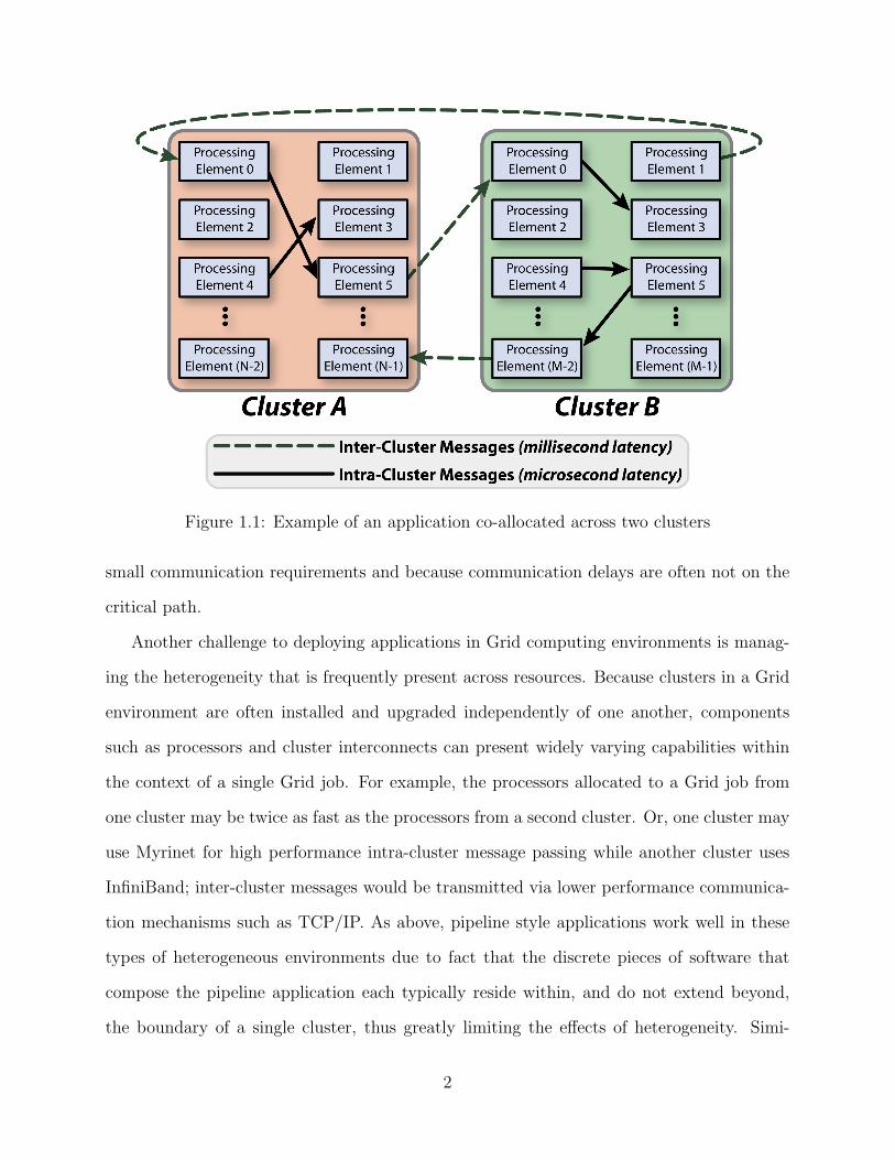
Figure 1.1: Example of an application co-allocated across two clusters
small communication requirements and because communication delays are often not on the
critical path.
Another challenge to deploying applications in Grid computing environments is manag-
ing the heterogeneity that is frequently present across resources. Because clusters in a Grid
environment are often installed and upgraded independently of one another, components
such as processors and cluster interconnects can present widely varying capabilities within
the context of a single Grid job. For example, the processors allocated to a Grid job from
one cluster may be twice as fast as the processors from a second cluster. Or, one cluster may
use Myrinet for high performance intra-cluster message passing while another cluster uses
InfiniBand; inter-cluster messages would be transmitted via lower performance communica-
tion mechanisms such as TCP/IP. As above, pipeline style applications work well in these
types of heterogeneous environments due to fact that the discrete pieces of software that
compose the pipeline application each typically reside within, and do not extend beyond,
the boundary of a single cluster, thus greatly limiting the effects of heterogeneity. Simi-
2

larly, master-slave style applications also work well in heterogeneous environments because
each slave works independently, returning results as fast as it is capable and communicating
minimally with other slaves.
In contrast, some classes of applications present serious challenges to deployment in Grid
computing environments. Tightly-coupled applications in which every processor in a com-
putation performs the same task and communicates with some subset of all processes in
the computation during every iteration present a significant challenge. Examples of such
applications include most simulations of physical systems in science and engineering, for ex-
ample structured and unstructured mesh applications and applications from domains such
as molecular dynamics or cosmology in which elements in a three-dimensional space interact
with all other elements within a specified cutoff distance. Optimizing these types of applica-
tions through techniques such as masking the effects of wide-area latency and managing the
heterogeneity of resources is critical for achieving good performance in Grid environments.
To date, however, much of the work involving the deployment of tightly-coupled applications
on computational Grids has focused on algorithm-level optimizations, such as the expansion
of ghost zone regions in mesh computations [8].
1.1 Example Grid Computing Environments
The rapid growth in the use of Grid computing for solving large-scale scientific problems is
driven by a number of developments in several related and overlapping areas. For example,
the recent trend in building computational clusters from commodity off-the-shelf components
has resulted in a proliferation of dispersed pockets of significant computational power owned
by individual organizations. Connecting these dispersed pockets of computational power is
a natural next step. Developments of this nature set important directions and guidelines for
research like that presented in this thesis. To that end, the following two examples highlight
environments in which the work presented in this thesis might be applied directly.
3

The first example environment in which the work described in this thesis might be appli-
cable is that of a circumscribed campus-area network. Due to the increasing use of cluster
computing, individual departments are now able to afford to own not-insignificant amounts
of computational power which are leveraged towards unique departmental goals. However,
the sizes of these departmentally-owned computational resources are often limited either by
the availability of funding or by the infeasibility of purchasing clusters that far exceed the
expected steady-state cycle needs of the department. One can envision a situation in which
two collaborating departments on the same campus might want to join their individually-
owned cluster resources together for the purpose of solving occasional very large problems.
Certain challenges to Grid computing are not as severe in this type of environment. Because
communication is generally limited to a campus-area network, cross-cluster latencies in a
Grid computing environment of this nature are typically on the order of one to three mil-
liseconds. While this is still bad compared to the microsecond-scale latencies within a single
cluster, latencies of this scale are much more easily masked than the latencies in national
scale Grid environments where latencies are measured in tens of milliseconds. On the other
hand, other challenges to Grid computing might be very obvious in this type of environment.
For example, because individual departments often purchase clusters independently, issues
of heterogeneity, in terms of processor speeds or communication interconnects, might be
difficult to manage.
The second example environment in which the work described in this thesis might be
applicable is that of established Grid computing environments such as the TeraGrid [1]. The
TeraGrid is a multi-year effort, led by the National Science Foundation and involving nine
core sites distributed across the United States, to build and deploy the world’s largest and
fastest Grid computing environment available for open scientific research. The core TeraGrid
includes over one hundred teraflops of computational power and over fifteen petabyte of disk
storage, interconnected with a forty-gigabit-per-second national network. Figure 1.2 shows a
map of the core TeraGrid infrastructure. Such an environment presents different challenges
4

Figure 1.2: Map of the NSF TeraGrid Extensible Terascale Facility core sites [1]
from ones described in the example of a campus-area network. Because the TeraGrid is a joint
effort among several collaborating sites with the express purpose of fostering Grid computing,
issues such as heterogeneity have been kept to a minimum, particularly in the context of
the original core TeraGrid resources. On the other hand, because the TeraGrid environment
spans the United States, overcoming challenges such as cross-site latencies measured in tens
of milliseconds becomes critical when optimizing tightly-coupled application performance.
1.2 Grid Computing Challenges
Viewing Grid computing in the contexts described above is useful because it allows the
challenges to efficiently executing tightly-coupled parallel applications in such environments
to be identified. This section specifically states several of these challenges.
• Wide-area communication costs – In environments consisting of resources sepa-
rated by large geographic distances, such as in the case of the TeraGrid, the efficiency
of communication taking place over the wide-area is a critical factor to consider when
5

optimizing application performance. Two issues related to communication costs are
important: bandwidth and latency. Of these two issues, latency seems to be the more
challenging. Challenges involving bandwidth may often be resolved simply by building
a more capable infrastructure that can deliver more bandwidth to applications. For
example, the backbone connections in the TeraGrid bond four ten-gigabit-per-second
channels together to deliver forty gigabits-per-second. It seems likely that if, in the
future, applications demand additional bandwidth to feasibly run on the TeraGrid,
that additional bandwidth could be requisitioned. Latency, on the other hand, has
a lower bound between any two points on the TeraGrid due to the simple physics of
nature; light only travels so fast.
• Efficient mapping of work to resources – Some success has been made in using
algorithm-specific optimizations for achieving good performance of various types of
tightly-coupled problems in Grid computing environments. Work representative of
these efforts is described in Chapter 3. A downside of this type of approach is that
these types of optimizations may be quite complex for a programmer to implement
correctly. Further, optimizations of this nature may lead to optimizing an application
specifically for a particular Grid environment, requiring frustrating modifications to the
optimized implementation in order to move it to a different Grid environment at a later
time. For example, consider an unstructured mesh decomposition specifically coded
to map work evenly among two clusters in a Grid. In contrast to applications such
as master-slave decompositions in which work can readily be parceled out to available
processors, manually partitioning an unstructured mesh for efficient execution over a
Grid is non-trivial due to the complexities involved in locating good division points in
the mesh that result in approximately-equal work on both clusters while simultaneously
minimizing communication costs between the clusters. Further, the manual mapping
of work must be changed if, in the future, changes are made to the environment in
6

which the application runs, such as by upgrading the nodes in one cluster to be of
a faster speed, requiring more work to be mapped to these processors relative to the
slower processors in the other cluster, or by introducing a third cluster across which
the application is mapped.
• Dynamic environment – By their very nature, Grid computing environments are
extremely dynamic. For example, latencies between parts of a computation may in-
crease or decrease depending on other competing network traffic. Effectively dealing
with the issues surrounding this dynamic nature of Grids is crucial for achieving good
application performance. Optimizing applications to run efficiently in response to
these challenges is difficult because it requires software to be able to adaptively tune
application performance at runtime.
• Pervasive heterogeneity – Many Grid computing environments, such as those com-
posed of organizations that combine resources “after the fact” of purchasing equipment
independently, contain pervasive heterogeneity. This is in contrast to proscribed Grid
environments like the core TeraGrid which are developed specifically to minimize is-
sues of heterogeneity. In the environments, heterogeneity in the form of processors
of different speeds and capabilities as well as multiple types of cluster interconnects
(e.g., Myrinet and InfiniBand) will be common. To achieve maximum performance of
tightly-coupled codes running in such an environment, this heterogeneity needs to be
managed.
1.3 Thesis Objectives
The objective of this thesis is to examine the feasibility of deploying tightly-coupled par-
allel applications in Grid computing environments. A desired outcome of this work is the
capability of delivering application performance in a Grid environment that is on par with
7

the performance within a single cluster while at the same time requiring few or no modi-
fications to the application software. To that end, the thesis explores techniques that can
be deployed effectively at the runtime system (middleware) level and used in a Grid com-
puting environment consisting of multiple clusters. Such techniques include capabilities for
efficiently mapping work to the resources allocated to a Grid application and dynamically
updating this mapping in light of short-term changes in these resources (e.g., a sudden and
unexpected increase in latency between two clusters across which a Grid job is co-allocated).
Additional techniques address issues related to the heterogeneity found in a Grid environ-
ment, such as by providing abstractions to the various interconnects used throughout all
resources in a Grid job or by partitioning a Grid job to reflect processors of different speeds
or capabilities. An advantage of developing these techniques within the runtime system is
that they are automatically available to applications representing a wide variety of problem
decomposition strategies with little or no effort required by application developers. This en-
ables application developers to focus on the underlying problem, writing a software solution
in the most straightforward way possible, without being concerned with details of the Grid
environment in which the application will be deployed.
This thesis promotes a message-driven programming model for developing Grid applica-
tions. A message-driven model, as realized in systems such as Charm++ [21] and Adaptive
MPI [20], is attractive for use in Grid computing because it encourages a development style
in which an application is broken into a large number of parallel migratable objects which
are subsequently mapped onto a much smaller number of physical processors by an adaptive
runtime system. The runtime system can provide features such as message prioritization
and dynamic load balancing, allowing the runtime system to optimize a computation dur-
ing execution. A message-driven runtime system architecture coupled with optimization
capabilities allows an application to be feasibly deployed in Grid environments consisting
of several clusters that are made up of processors of various speeds and utilizing multiple
network interconnects.
8

Chapter 2
Enabling Technologies
This chapter describes the enabling technologies upon which the work in this thesis is based.
These technologies include the Charm++ and Adaptive MPI runtime systems and the soft-
ware surrounding them as well as the Virtual Machine Interface message passing layer.
2.1 Charm++ and Adaptive MPI
Charm++ [21] is a message-driven parallel programming language based on C++ and de-
signed with the goal of enhancing programmer productivity by providing a high-level ab-
straction of a parallel computation while at the same time providing good performance on
platforms ranging from traditional supercomputers to more recent commodity cluster envi-
ronments. Charm++ is backed by an adaptive runtime system that provides features such
as processor virtualization, prioritized message delivery, load balancing, and optimized com-
munication libraries, especially for collective operations such as broadcasts and reductions.
Programs written in Charm++ consist of parallel objects called chares that communicate
with each other through asynchronous message passing. When an object receives a message,
the message triggers a corresponding entry method within the object to handle the message
asynchronously. Further, objects may be organized into one or more indexed collections
called chare arrays. Messages may be sent to individual objects within a chare array or to
the entire chare array simultaneously.
The chares in a Charm++ program are assigned to processors by the runtime system,
and this mapping is transparent to the user. Figure 2.1 illustrates the concept that the
9

Figure 2.1: Depiction of the user’s view of a Charm++ application and the system’s viewafter mapping objects to processors
user’s view of a Charm++ computation usually varies greatly from the way that the com-
putation is mapped onto physical resources. The user views the computation in terms of the
object-based abstraction, simply invoking methods on objects within the computation. The
runtime system’s view of the system is quite different, however, because it includes details
about object placement and about the messages sent between objects that correspond to
method invocations made by the user. Because the object-to-processor mapping is transpar-
ent to the user, the runtime system may change this assignment dynamically by migrating
objects among processors. A suite of measurement-based load balancers is provided to take
advantage of this capability. In addition, the migration capability is leveraged to support
other capabilities such as automatic checkpointing, fault tolerance, and the ability to shrink
and expand the set of processors used by a parallel job.
Adaptive MPI (AMPI) [20] provides the same capabilities as Charm++ in a more familiar
MPI programming model. AMPI implements the MPI standard by encapsulating each MPI
process within a user-level migratable thread. By embedding each thread within a Charm++
object, AMPI programs can automatically take advantage of the features of the Charm++
runtime system with little or no changes to the underlying MPI program. This is very
attractive for the work presented in this thesis due to the large number of MPI applications
available representing a wide-variety of styles of problem decomposition that may be readily
10
deployed into Grid environments without requiring modification of application code.
The message-driven model used in the Charm++ runtime system is similar to the model
used in systems such as Active Messages [48, 49], Fast Messages [40], and Nexus [13, 14]. A
key idea with Charm++, however, is that a programmer completely decomposes a program
into a large number, tens or hundreds, of Charm++ chares or AMPI threads per physical
processor, allowing the runtime system to adaptively overlap computation in ready objects
with communication taking place in objects waiting for remote data. These objects can in
some ways be thought of as virtualizing the notion of a processor [22]. This use of processor
virtualization is similar to virtualization used in systems such as the CM-2 [2].
2.2 Virtual Machine Interface
The proliferation of high-performance clusters built from commodity off-the-shelf compo-
nents has resulted in the widespread use of several high-bandwidth low-latency cluster inter-
connects such as Myrinet [6] and InfiniBand [44]. Because these types of interconnects deliver
very good hardware performance, increased emphasis has been placed on the efficiency of the
underlying messaging software. Delivering point-to-point communication performance near
what is achievable from the raw network hardware is now the primary goal to message layer
designers. Furthermore, messaging layers are now expected to address several secondary
goals including portability, monitoring and management, and support for applications run-
ning in distributed Grid computing environments.
The Virtual Machine Interface (VMI) message layer [42, 41] is designed to be a low-
overhead abstraction layer providing several compelling features:
• Multiple interconnects – VMI is designed to provide a single programming interface
to the various network interconnects commonly used in high-performance commodity
clusters. Software implemented on VMI immediately gains access to all of the intercon-
nects supported by VMI while paying a small overhead of only a few microseconds per
11

message. Furthermore, the underlying network interconnect may be switched simply
by changing the contents of a file that describes the devices used for the computation;
no recompilation or relinking of the application software is necessary.
• Data striping and automatic fail-over – Because VMI operates as a software layer
directly above the native network interconnect layer, it can stripe data across multi-
ple network interconnects, even if these network interconnects are heterogeneous. By
striping data across multiple network interconnects, VMI can deliver the aggregate
bandwidth available from all interconnects to the application. Furthermore, if one in-
terconnect fails, VMI can simply continue operating with any remaining interconnects.
• Portability – VMI is designed to be portable in two ways. First, VMI is designed to
be portable to a wide variety of network interconnects. The challenge to this goal is
the difficulty in designing a single Application Program Interface that can encompass
all of the lower-level network APIs currently available while simultaneously providing
excellent performance by giving the programmer access to some of the unique features
of individual interfaces. Second, VMI is designed to be portable to a wide variety of
platforms. Currently, VMI is available on IA-32, IA-64, and PowerPC architectures.
• Scalability – As high-performance commodity clusters increase in popularity, there
is also a trend toward an increase in the number of nodes in a single cluster. Clusters
with hundreds or thousands of nodes are now common. To this end, VMI is designed
to scale to upward of several thousand nodes.
• Support for distributed Grid-based computing – The increasing number of clus-
ter installations within collaborating organizations has led to a growing desire to con-
nect multiple clusters together in order to harness the aggregate power of all machines.
The challenges to creating a messaging layer to address this goal are twofold. First,
the messaging layer must scale to hundreds or thousands of nodes, just like in the
12

case of building independent clusters that each contain a large number of nodes. Sec-
ond, the messaging layer must not only provide good performance for the variety of
interconnects used within each cluster but must also provide good performance for the
wide-area networks used to connect the clusters themselves together. Design decisions
regarding bandwidth and latency, for example, may be applicable to local area net-
works but not to the wide area. Because VMI is designed to be scalable to upward of
several thousand nodes and because it readily supports various types of interconnects,
it is a favorable platform for Grid computing. Furthermore, algorithms within VMI
are designed to be latency tolerant in order to allow VMI to function correctly over
wide-area networks.
• Dynamic monitoring and management – In order to deal with the ever-increasing
complexity of cluster and Grid computing environments, modern messaging layers add
support for monitoring and management. VMI includes capabilities for monitoring the
state of the messaging layer in real time and dynamically managing the state of the
entire network stack.
VMI achieves many of these goals by using an architecture in which software modules are
dynamically loaded at runtime. These modules are organized into a send chain and a receive
chain of modules, with all data that passes out of or into the messaging layer traveling
through the modules on the respective chain. Each module on a chain may simply pass
the data to the next module, modify the data in some way (for example, by compressing
or encrypting it), or “sink” the data by delivering it into the underlying network (in the
case of a device on the send chain) or into the application (in the case of a device on
the receive chain). This architecture leads to many novel possibilities. For example, as
described above, by loading multiple modules simultaneously, data may be striped across
multiple interconnects. This concept may be extended to allow a parallel application to run
in a Grid computing environment using a high-performance interconnect to communicate
13

with local neighbors within the computation and a wide-area network to communicate with
neighbors located on remote nodes.
One of the most important contributions of VMI is its ability to provide an abstract view
of the underlying network used by all parts of a distributed Grid computation. Underneath
this abstract view, however, may be a network consisting of several heterogeneous intercon-
nects. Using VMI, message data travels over the most efficient point-to-point connection
between any pair of processes in a Grid computation. Further, the overhead of this capability
is measured in a few microseconds per message. It is for this reason that VMI is a critical
part of the work surrounding this thesis.
2.3 Efficient Implementation of Charm++ on VMI
VMI is not typically intended to be a software layer exposed directly to application devel-
opers, but rather as a layer upon which higher level message layers or runtime systems can
be built. To this end, earlier work [34] describes an efficient implementation of Charm++
that uses VMI as its underlying message passing layer. This implementation is significant
to the work described in this thesis because it delivers the features of VMI described in Sec-
tion 2.2 to Charm++ and AMPI applications without requiring any additional effort on the
part of the application developer. In light of the challenges to Grid computing described in
Section 1.2, probably the most important contribution that the efficient implementation of
Charm++ on VMI provides is abstracting the details of the various underlying interconnects
used in all parts of a Grid computation. That is, an application can run across two clusters
using, for example, Myrinet for communication in one cluster, InfiniBand for communication
in the other cluster, and TCP/IP for inter-cluster communication. All communication be-
tween any pair of processes in the computation travels over the most favorable interconnect
possible.
Figure 2.2 shows the structure of the Charm++ implementation on VMI. Charm++
14

Figure 2.2: Structure of the efficient implementation of Charm++ on VMI
is implemented in terms of Converse, a portable foundation for higher-level language and
library writers. Converse includes a set of functions, the Converse Machine Interface, that
define the base functionality that must be implemented to port Charm++ to a new archi-
tecture. The implementation of Charm++ is written in terms of this Converse Machine
Interface, requiring few modifications to the core Charm++ software itself.
Using the implementation of Charm++ on VMI as a basis for the work in this thesis
provides several useful possibilities. For example, the following section describes a VMI
“delay device” that can induce arbitrary artificial latencies between pairs of processes in
a computation. This delay device allows simulating a Grid environment with any desired
latencies using a single cluster.
15

2.4 Artificial Latency Environment
Because running an application in a real Grid environment does not permit varying the
wide-area latency as necessary to carry out experiments, the features of VMI can be used
to create a “simulated Grid environment” physically consisting of nodes from a single real
cluster. In this simulated Grid environment, arbitrary latencies can be inserted between any
pair of nodes, allowing cross-cluster latencies to be swept across a range to study the impact
of varying wide-area latencies on the underlying application. Creating such an environment
leverages the implementation of Charm++ running on the Virtual Machine Interface mes-
saging layer. Recall that a novel feature of VMI is the ability to organize the device driver
software modules used for communication operations into send and receive chains of drivers.
As message data travels along a chain, each module on the chain may simply pass the data
to the next module, manipulate the data in arbitrary ways, or deliver the data into the un-
derlying network. This capability of intercepting message data is used to write a VMI device
driver that injects pre-defined latencies between arbitrary pairs of nodes. This “delay device
driver” is then inserted into the VMI device chains used for experiments by constructing
send and receive chains that consist of two network drivers with the delay driver in between.
By affiliating a subset of the cluster’s nodes (i.e., those that exist on the “local cluster”) with
the first driver in the chain, message data are immediately sent between the nodes within
that subset without passing through the delay device. For nodes not in this affiliation (i.e.,
those that exist on the “remote cluster”), messages are intercepted by the delay device which
delays the message by a pre-defined amount of time before passing it to the network device
driver used to communicate over the “wide area.”
The VMI delay device carries out its work on the receive side of a communication channel.
When message data arrives at the delay device, the driver inserts the data along with the
arrival time into a linked list of delayed messages. As the runtime system periodically
“pumps” the message layer for new messages, the timestamp for the element at the head of
16

the list is examined. If the current time is greater than the head element’s arrival time plus
the pre-defined artificial latency, the message is released to the runtime system for delivery.
Because messages are timestamped in the order that they are received, only the head of the
list needs to be examined for each “pump” operation; all elements following the head are
necessarily received after the head element.
Creating the artificial latency environment used for the experiments in this thesis involves
few changes to the software stack used in real Grid environments. That is, the application,
runtime system, messaging layer, and underlying communication layers are all the same
both in experiments using the artificial latency environment and in experiments running
in real Grid environments; only the introduction of the delay device driver is necessary to
construct the artificial latency environment. For this reason, experiment results collected in
the artificial latency environment closely match results collected in real Grid environments.
In particular, the results for the case studies presented in Chapter 8 show very similar
performance for parallel applications running in both environments.
17

Chapter 3
Related Work
The work described in this thesis shares characteristics with several other projects while at
the same time offering its own unique contributions. This chapter describes related work
and draws comparisons and contrasts to the work described in this thesis.
Viewing a distributed computation as a set of interacting objects and, accordingly, using
object oriented programming techniques to manage complexity is an attractive approach
to Grid computing. Several other projects such as Legion [16] and Globe [47] share this
characteristic with the work presented in this thesis. In contrast, however, both of these
projects tend to be focused more on the entire range of problems surrounding Grid com-
puting, including resource management, file and data access, information brokering, and
security. Indeed, the designers of Legion call such an all-encompassing system a metasys-
tem. Examples of applications running in these kinds of environments appear to be focused
on those types that can implicitly tolerate latency, such as parameter sweep applications [39],
or applications such as molecular dynamics applications running entirely within the context
of a single machine on the Grid [38]. The goal of this thesis differs from this type of work
in that this thesis is specifically focused on the topic of developing techniques for efficiently
executing tightly-coupled applications that are co-allocated across multiple resources in a
Grid environment.
Several projects extend the MPI parallel computing standard to work in a Grid envi-
ronment with the goal of allowing jobs that can span multiple clusters. Examples of such
projects include MPICH-G2 [24] and MPICH/MADIII [4]. These projects, like the work
described in this thesis, view the communication infrastructure of a distributed Grid job
18

as a hierarchy of interconnects. Such a view consists of high-performance local-area inter-
connects such as Myrinet or InfiniBand at one level of the hierarchy and lower-performance
wide-area interconnects such as TCP/IP at another level of the hierarchy. The goal is to
allow any pair of processors to communicate via the most efficient channel possible within
the hierarchy. MPICH-G2 achieves this goal by being layered on top of underlying native
MPI implementations within each cluster to provide efficient intra-cluster communication
and by using TCP/IP to provide inter-cluster communication. MPICH/MADIII takes an
approach that is very similar to the implementation of Charm++ on VMI described in Sec-
tion 2.2. MPICH/MADIII is implemented on top of a communication library, Madeleine
III, that allows multiple underlying networks to be used in a way similar to VMI. Further,
MPICH/MADIII uses an efficient user-level thread library, Marcel, that provides task de-
composition capabilities similar to what is available with Charm++ objects or Adaptive MPI
threads. In contrast to MPICH/MADIII, however, the work described in this thesis seeks
to increase the number of opportunities for the adaptive runtime system to overlap useful
computation with communication by using very large degrees of virtualization, with perhaps
hundreds of objects per physical processor in the computation. MPICH/MADIII seems to
typically use a much smaller number of threads per processor. Further, the Charm++
adaptive runtime system includes the ability to dynamically load balance objects within a
distributed computation while MPICH/MADIII does not seem to offer this functionality.
This capability is important for achieving good performance on fine-grained Grid computa-
tions that span multiple clusters.
Various algorithm-level approaches to tolerating latency in Grid computing environments
exist. For example, the performance of Partial Differential Equation solvers running in a
Grid environment may be improved by increasing the number of ghost cell layers used per
processor [8]. Increasing the number of ghost zones allows each processor to buffer more
data and reduces the number of messages sent between processors. Further improvements
to the PDE algorithm allow the elimination of diagonal communications. Together, these
19

algorithm-level optimizations allow the performance of the application described in the cited
paper to be improved by as much as 170%. The primary contrast between approaches such
as the one described in the paper and the work described in this thesis is that the techniques
described in this thesis operate at the runtime system layer rather than at the application
layer. While algorithm-level approaches have the advantage that they can generally achieve
very good levels of optimization, runtime-level approaches have the advantage that they are
broadly available to a wide variety of problem decomposition types (i.e., structured and un-
structured mesh decomposition, spatial decomposition, etc.) without requiring modification
of application software.
Cactus-G [3] is a Grid-enabled computational framework that is based on the Cactus
problem solving environment and the MPICH-G2 message passing library. Originally de-
signed for use in numerical relativity applications such as modeling black holes, neutron stars,
and gravitational waves, Cactus has grown into a framework well-suited to solving general
mesh decomposition problems. A novel feature of Cactus is that it consists of a central core
called the flesh which connects to application modules called thorns through an extensible
interface. The thorns in a computation encapsulate the actual scientific code governing the
application as well as capabilities such as parallel I/O, data distribution, and checkpointing.
The experiment described in the paper leverages this rich platform to perform an experiment
in which a heterogeneous environment consisting of four machines distributed between the
San Diego Supercomputing Center (SDSC) and the National Center for Supercomputing
Applications (NCSA) is synthesized and applied to a tightly-coupled mesh decomposition
problem. The authors are successful in this endeavor due to the ability to leverage thorns
that optimize the computation in three ways. First, because the resources physically allo-
cated to the computation consisted of one machine at SDSC and three machines at NCSA,
the authors positioned the gridpoints in the mesh to reflect this uneven distribution. Sec-
ond, the authors increased the size of the ghost zone layers on each processor similar to the
method used in the ghost zone expansion technique described above [8]. Third, the authors
20
used a thorn to compress message data that were sent over the wide-area connection between
SDSC and NCSA. In many ways, Cactus-G can be thought of as an elaborate runtime system
that offers features similar to those found in the Charm++ runtime. The work described
in this thesis differs from the work in Cactus, however, in that the approach taken by this
thesis focuses on dividing a computation into a large number of objects and then dynam-
ically mapping and re-mapping these objects onto physical processors as the computation
progresses. In many senses, this approach is at a lower level in the software stack than the
approach taken by Cactus-G.
Load balancing of parallel applications is a well-known concept with a history dating
back more than twenty years. For example, Fox describes load balancing through the use of
randomized placement of sub-blocks within a problem [15]. Interest in load balancing has
increased in recent years in the field of Grid computing because the performance of Grid
applications can be significantly improved through the use of good load balancing. Two
primary ways of doing Grid load balancing exist: static techniques and dynamic techniques.
When using static techniques, decomposed pieces of an overall problem are assigned to the
most suitable (least loaded) processor in the computation. However, once a unit of work is
placed on a processor, it remains on that processor until the work is completed; it cannot
migrate to a new processor as is possible with the Charm++ runtime system. Frequently,
static load balancing techniques cannot fully address the unique needs of Grid environments
due to the constantly-changing nature of Grids. To that end, the work presented in this
thesis focuses on dynamic load balancing techniques provided by the Charm++ runtime
system [55].
The dynamic load balancing capabilities of the work described in this thesis are similar
to systems such as OptimalGrid [30] which monitor the runtime performance of each node
in a computation with respect to the portion of a problem that it is handling and reap-
portion successive iterations of the computation to address load imbalances. A particularly
in-depth analysis of this type of technique was carried out using a Successive Over-Relaxation
21

(SOR) mesh problem running in the PlanetLab Grid environment [9]. The biggest difference
between the dynamic load balancing research in OptimalGrid and in the PlanetLab experi-
ments and the work in this thesis is that the work presented here balances a computation in
terms of both measured CPU utilization and the object-to-object communication graph of
the computation in relation to the structure of the Grid resources used by the computation.
The common thread that differentiates the work described in this thesis from others is the
pervasive use of message-driven execution, in the form of Charm++ chares or AMPI threads,
coupled with Grid topology-aware dynamic load balancing as a means of tolerating latency
in Grid computing environments without requiring modification of application software.
22

Chapter 4
Adaptive Latency Masking
Perhaps the most important factor for successfully running tightly-coupled applications in
Grid environments is the ability to mask the effects of cross-site latency on the portions
of the computation that communicate across the wide area. Many parallel applications
are written in a way so as to minimize the effects of latency, at least to some degree.
For example, a common way of structuring MPI applications is to arrange each timestep
such that each processor asynchronously sends data in ghost cells at the borders of the
processor’s portion of application data to its neighbors in the computation, then performs
its computation required to complete the timestep, and finally receives the data necessary to
compute the next timestep from its neighbors in the computation. Thus, the time required
to communicate a processor’s data to its neighbors is partially masked by the time used by
the processor to perform its computation in the timestep. This solution, while helpful in
traditional parallel computing environments, is less useful in Grid environments because the
degree to which latency can be masked within the application varies only with the number
of processors used to decompose the problem. While this may be worthwhile within the
context of a single parallel machine with microsecond latencies between processors, it may
be much less worthwhile in a Grid environment in which inter-processor latencies may be tens
of milliseconds between some processor pairs. Further, the solution requires the application
programmer to carefully structure the application software itself to achieve latency masking,
and this may make the software much more complicated than it otherwise would need to be.
This chapter describes how the architecture of the Charm++ runtime system itself can
be used to mask the effects of latency on tightly-coupled parallel applications running in Grid
23

environments. The technique described here is especially attractive because it takes place
automatically within the runtime system, allowing the application programmer to structure
the application in a more straightforward manner that does not need to take the deployment
environment into consideration. More importantly, however, the number of objects used to
decompose a Charm++ program does not depend on the number of processors on which
the application is running. This means that the number of objects can be varied to give the
application a higher degree of latency tolerance.
4.1 Adaptive Latency Masking in Grid Environments
The fundamental idea behind the Charm++ runtime system is that a programmer divides
a program into a large number of message-driven entities, implemented in the form of either
Charm++ objects or Adaptive MPI virtual processors. The number of objects or virtual
processors is independent of, and in practice much larger than, the number of physical
processors. The runtime system maps objects onto physical processors and may dynamically
adjust this mapping as the application executes to balance load or optimize communication
costs. Rather than thinking in terms of physical processors, the programmer thinks in terms
of the object abstraction and writes code to coordinate interactions among these entities.
These interactions are realized as asynchronous messages that are passed between physical
processors in the computation. As messages arrive at a physical processor, they are enqueued
in a message queue in either FIFO or priority order. When a physical processor becomes
idle, its message scheduler dequeues the next waiting message and delivers it, triggering
the execution of code that is encapsulated within an object to handle the message. This
code runs to completion, producing other messages for objects on this or another physical
processor.
Because messages are asynchronous, the runtime system may schedule the execution of a
new object immediately after execution within an existing objects completes, resulting in one
24

Figure 4.1: Hypothetical timeline illustrating the use of message-driven objects to toleratewide-area latency
or more messages sent by the object. Rather than waiting for these messages to be delivered,
the newly-scheduled object begins work immediately, thus overlapping its computation with
the communication of the previous object. This ability to overlap useful computation with
communication is important within the context of a single parallel machine, but is especially
critical for applications that are running in a Grid environment in which nodes are separated
by a high-latency wide-area network. Figure 4.1 illustrates this concept by depicting a
hypothetical timeline for three processors running on two clusters that are connected by
a high-latency wide-area network. Processors A and B are located within one cluster and
processor C is located within the second cluster. At the left side of the timeline, processor
B sends a message to processor C; this message must cross the high-latency inter-cluster
network. Rather than waiting idly for this message to be delivered, B is free to respond to
incoming messages from processor A, and in fact performs several short computations and
message exchanges with A. Finally, processor C responds to processor B with the result of
the computation previously triggered by B. The important idea is that B is able to do useful
work during the gap between dispatching a message to C and receiving a response.
Issues related to adaptivity and granularity in Charm++ programs have been studied
extensively [23, 17, 22, 18] and are important to the discussion in this chapter. The cited
25

papers report that the overhead associated with scheduling a Charm++ object invocation
is small, less than a microsecond, and that the most critical factor in determining an ap-
propriate grainsize for Charm++ applications is the communication overhead. Figure 4.2
illustrates this concept by showing the execution time of a hypothetical parallel applica-
tion as a function of grainsize. For small grainsizes, where a large number of objects are
used to decompose the problem, execution time is relatively large due to a large amount
of overhead spent in communication. As grainsize increases and approaches GL, execution
time decreases rapidly. This is because the problem is divided among a smaller number of
objects, with each object working on a larger portion of the problem space, thus requiring
less communication. Throughout the flat region of the graph, between GL and GH , execu-
tion time remains essentially unchanged because the overhead of communication is only a
small fraction of the overall execution time. Finally, when grainsize increases beyond GH ,
execution time once again increases significantly due to insufficient parallelism resulting in
wasted idle time. The important conclusion drawn in the cited papers is that the grainsize
in Charm++ programs should be as small as possible while still masking overhead. This
allows the number of objects used to decompose a problem to be independent from the
number of processors upon which the problem runs, giving the Charm++ runtime system
the maximum amount of freedom in mapping objects to processors.
4.2 Example Application: Five-Point Stencil
To examine the effectiveness of using the Charm++ runtime system’s message-driven execu-
tion model to mask latency, a simple five-point stencil finite difference method, also known
as a two-dimensional Jacobi decomposition (Jacobi2D), was examined in a simulated Grid
environment consisting of two clusters separated by a high-latency wide-area connection.
This simulated Grid environment is constructed using the VMI artificial latency environ-
ment described in Section 2.4. In this class of numerical method, a multidimensional mesh
26

Figure 4.2: Execution time of a parallel application as a function of grainsize [23]
is repeatedly updated by replacing the value at each point with some function of the values
at a small, fixed number of neighboring points. In the case of the experiment described
here, the neighboring points taken into consideration are the ones directly above and below
as well as to the left and right of a given cell. This produces four discrete communication
events per cell for each time-step.
For the experiment here, meshes of size 2048x2048 and 8192x8192 cells are considered.
The problem is decomposed using Charm++ objects by dividing the cells within the mesh
evenly among a specified number of objects. For example, for an 8192x8192 mesh divided
among 256 objects, 16 objects are mapped along each axis of the mesh. Accordingly, each
object has a 512x512 square section of the mesh to operate upon. During each time step,
each object communicates values for a 512x1 vector of cells to its appropriate neighbor.
Figure 4.3 graphically depicts this example problem layout.
The mesh is divided in half and split across two clusters separated by a wide-area connec-
tion, causing every time step to involve some objects communicating with neighbors situated
27

Figure 4.3: Graphical depiction of a five-point stencil decomposition in which a fixed numberof cells are divided across a variable number of objects
across the wide area. More importantly, however, both clusters contain a large number of
objects that communicate with neighbors solely within the local cluster. The expectation is
that the message-driven execution model will allow the high-latency communication opera-
tions to be masked by other communication that is carried out with neighbors situated on
the local cluster.
The five-point stencil is an attractive problem to consider because it allows a varying
degree of virtualization to be readily chosen by increasing or decreasing the number of objects
used to decompose the mesh for a fixed number of processors. Thus, the effectiveness of using
message-driven objects to mask the effects of latency can be more readily understood than
in the case of most applications in which the number of objects used is directly related to
the problem size and does not vary with the number of processors. Further, because the
problem is of a fixed size, always 2048x2048 or 8192x8192 cells, as the number of physical
processors increases the granularity of the portion of the problem residing on each processor
decreases. This fact allows conclusions to be drawn related to the impact of granularity on
the ability to mask wide-area latency to be made.
Figure 4.4 shows the results for the stencil decomposition on a 2048x2048 mesh for 8,
28

16, 32, and 64 physical processors. For each number of physical processors, the number of
objects used to decompose the mesh is varied by the square of increasing powers of 2. This
is due to the geometry of how objects are arranged over the mesh. For example, for the
case of 8 physical processors, 16, 64, 256, and 1024 objects are used to decompose the mesh,
corresponding to object arrangements of 4x4, 8x8, 16x16, and 32x32 objects.
For the case of 8 physical processors (Figure 4.4(a)), the number of objects is varied
from 16 to 1024 objects. For the 16 object case in which only two objects reside on each
physical processor, the per-step execution time of the application increases steadily as latency
increases. For this configuration, half of the objects on each side of the cross-cluster partition
must make a wide-area communication operation during each iteration. Further, because
each processor only holds two objects, little or no useful work may be overlapped with this
communication. As the number of objects per processor is increased, however, the effects
of wide-area latency can begin to be effectively masked. For the 64 object case in which
8 objects reside on each processor, the per-step execution time of the application remains
flat as the cross-cluster latency increases from 0 milliseconds to 8 milliseconds. This is
because useful work in objects that have only local communication requirements may be
used to overlap the otherwise-wasted communication time in objects that communicate with
neighbors across the cluster boundary. After latencies of 8 milliseconds, however, the amount
of locally-driven work per processor is exhausted and the slope of the line begins to increase
similar to the 16 object case. The latency tolerance of the 256 object case is even more
impressive. Although the per-step execution time for 256 objects is initially worse than the
per-step time for 64 objects, approximately 25 milliseconds per step for 256 objects versus
approximately 22 milliseconds per step for 64 objects, the 256 object line stays flat through
24 milliseconds of latency, thus resulting in a better per-step time than the 16 object case for
latencies greater than 16 milliseconds. For 256 objects on 8 processors, each processor has
32 objects to use for masking the effects of latency, and this provides many more possibilities
for overlapping work in ready locally-driven objects with cross-cluster communication time.
29

(a) Processors = 8 (b) Processors = 16
(c) Processors = 32 (d) Processors = 64
Figure 4.4: Performance of Jacobi2D 2048x2048 with Naive object mapping
Finally, for the case of 1024 objects, although the per-step execution time remains flat for
latencies 0 through 32 milliseconds, the per-step execution time of the application with 1024
objects, approximately 38 milliseconds per step, is much worse than the cases of fewer objects
per processor. This result indicates that the limits of virtualization have been reached and
that each processor cannot effectively make use of the much larger number of objects.
Because the problem size is fixed, always 2048x2048 cells, the granularity of the portion
of the problem residing on each processor decreases as the number of processors increases.
This is reflected in the graphs for 16 processors (Figure 4.4(b)), 32 processors (Figure 4.4(c)),
and 64 processors (Figure 4.4(d)) that show a decreasing trend in the per-step execution time
30

of the application as the number of processors increases.
In terms of latency tolerance, the graphs for 16, 32, and 64 processors show results that
are similar to the graph for 8 processors. That is, as the number of objects used to decompose
each problem is increased, the overall latency tolerance of the problem improves. This result
is reflected as horizontal segments in the per-step execution time plots for each number of
objects. Also similar to the case of 8 processors, the largest number of objects used per
processor (that is, 1024 objects for 16 processors, 4096 objects for 32 processors, and 4096
objects for 64 processors) results in worse per-step execution times for the application than
smaller numbers of objects. In these graphs for larger numbers of processors, however, it
is possible to notice an important phenomenon. After the “knee” in each plot where the
line shifts from horizontal to sloping sharply upwards as latency increases, the results for
the largest number of objects per physical processor show the best performance. While the
difference between the largest number of objects and a lower number of objects is subtle,
in the neighborhood of 500 microseconds per step, the phenomenon is consistently present
in the results for 16, 32, and 64 processors. This is an exciting result because it further
confirms that the Charm++ runtime system is masking the effects of cross-cluster latency
with useful work in the locally-driven objects on each processor.
As the number of processors increases, it is possible to observe another important idea
due to the decreasing granularity of the problem. As the granularity of the problem begins
to decrease, latencies above a certain point can no longer be tolerated, and this is reflected in
the location of the knee of each line on the graphs. For example, for the case of 8 processors
and 256 objects, the knee in the graph occurs at 24 milliseconds of latency. This corresponds
approximately to the per-step execution time of the problem for this number of objects. This
makes sense: after 24 milliseconds of latency, the amount of useful computation to be done
is less than the latency of wide-area communications. The time left over cannot be used
productively because there is no useful work to do in any object on each processor. This
idea is especially obvious as the number of processors increases and the per-step execution
31
times for the application fall well below the 32 milliseconds of latency at the righthand side
of the graphs. So, the overall observation is that the knee of the lower envelope of all curves
occurs near the per-step execution time of the application.
Figure 4.5 shows the results for the stencil decomposition on a 8192x8192 mesh for 8,
16, 32, and 64 physical processors. Because each side of the mesh is four times larger than
the mesh in the previous experiment, the overall problem involves sixteen times more work.
The expectation is that the per-step execution times for this problem size should be much
larger than before, and the graphs in the figure confirm this expectation. The results for the
larger problem size match the results for the previous problem in two important ways. First,
the plots corresponding to the lowest number of objects for each graph still show a steady
increase in the per-step execution time as latency increases. As before, this is due to each
processor holding only one or two objects and thus being unable to mask the effects of cross-
site latency in these cases. Second, the plots corresponding to higher numbers of objects for
each graph show improved latency tolerance characteristics until the limits of virtualization
are reached on each processor. There are many more cases of strictly horizontal lines for the
larger problem size, and this is because the per-step execution time of the application far
exceeds the range of latencies examined.
4.3 Summary
This chapter has introduced the concept of using the message-driven execution model of
the Charm++ runtime system as a way of masking the effects of latency between pieces
of a tightly-coupled parallel application co-allocated across geographically distributed Grid
resources. This latency masking happens automatically when each physical processor in
a Grid computation holds a large number of Charm++ objects or Adaptive MPI virtual
processors, allowing the runtime system to schedule work in ready objects during the time
required for messages to travel across high-latency wide-area connections. The fact that the
32
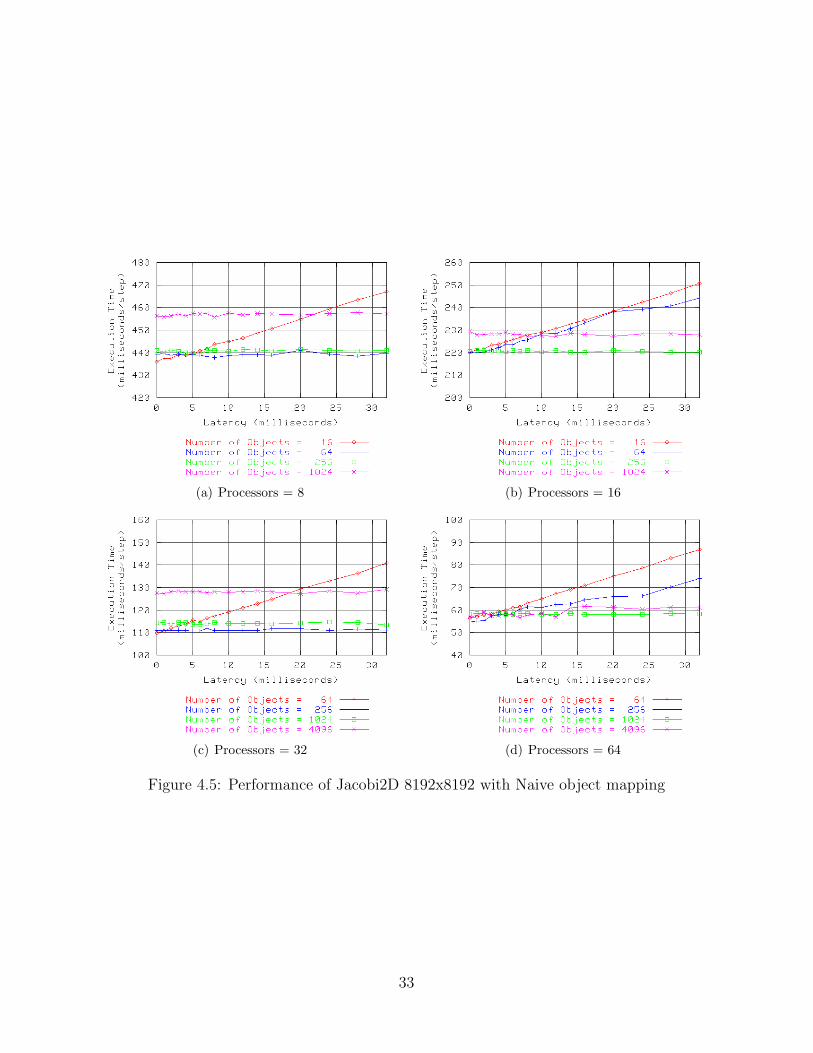
(a) Processors = 8 (b) Processors = 16
(c) Processors = 32 (d) Processors = 64
Figure 4.5: Performance of Jacobi2D 8192x8192 with Naive object mapping
33

technique is automatic is very attractive because it means that programmers receive the
capability of deploying applications in Grid environments “for free” without being required
to modify their software. In cases where an application is specifically modified for use in a
Grid environment, for example by modifying a mesh application to increase the number of
ghost zone regions to improve latency tolerance, the latency masking characteristics of the
Charm++ runtime system work with the application-specific modifications.
The technique presented in this chapter represents the primary architectural contribution
of this thesis in optimizing tightly-coupled parallel applications running in Grid computing
environments. In relation to this, the following three chapters build on the contributions of
this chapter in the form of techniques that represent optimizations to this architecture.
34
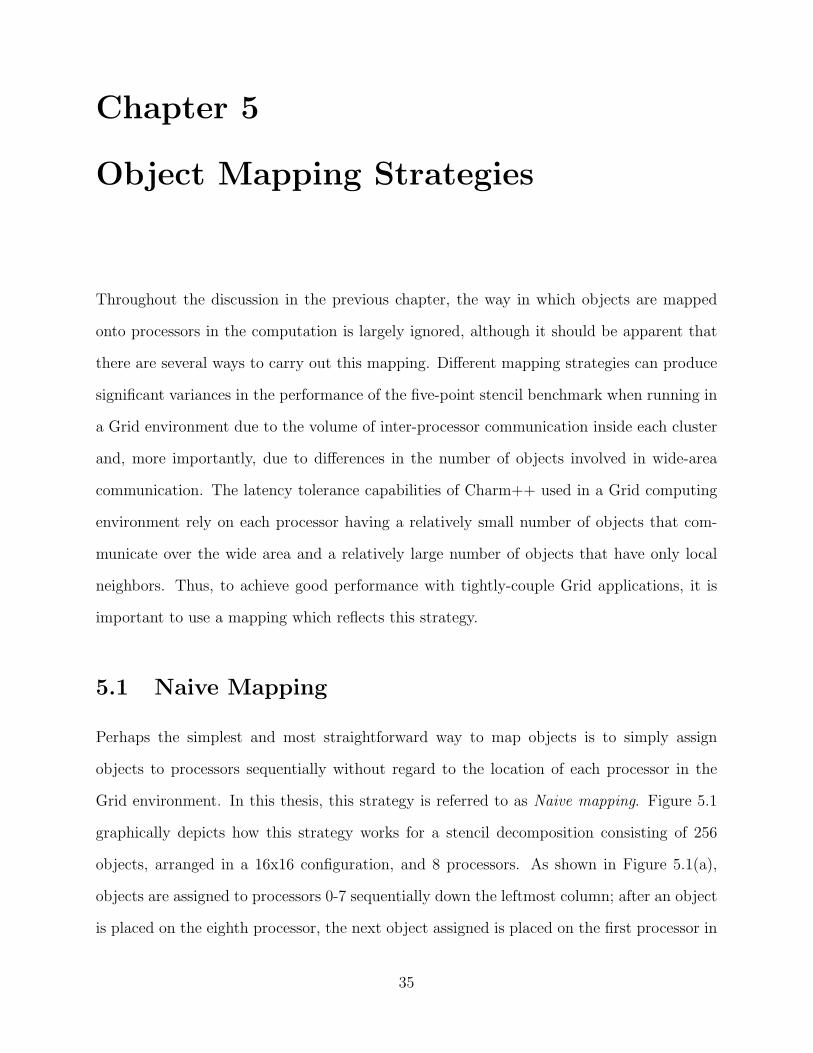
Chapter 5
Object Mapping Strategies
Throughout the discussion in the previous chapter, the way in which objects are mapped
onto processors in the computation is largely ignored, although it should be apparent that
there are several ways to carry out this mapping. Different mapping strategies can produce
significant variances in the performance of the five-point stencil benchmark when running in
a Grid environment due to the volume of inter-processor communication inside each cluster
and, more importantly, due to differences in the number of objects involved in wide-area
communication. The latency tolerance capabilities of Charm++ used in a Grid computing
environment rely on each processor having a relatively small number of objects that com-
municate over the wide area and a relatively large number of objects that have only local
neighbors. Thus, to achieve good performance with tightly-couple Grid applications, it is
important to use a mapping which reflects this strategy.
5.1 Naive Mapping
Perhaps the simplest and most straightforward way to map objects is to simply assign
objects to processors sequentially without regard to the location of each processor in the
Grid environment. In this thesis, this strategy is referred to as Naive mapping. Figure 5.1
graphically depicts how this strategy works for a stencil decomposition consisting of 256
objects, arranged in a 16x16 configuration, and 8 processors. As shown in Figure 5.1(a),
objects are assigned to processors 0-7 sequentially down the leftmost column; after an object
is placed on the eighth processor, the next object assigned is placed on the first processor in
35
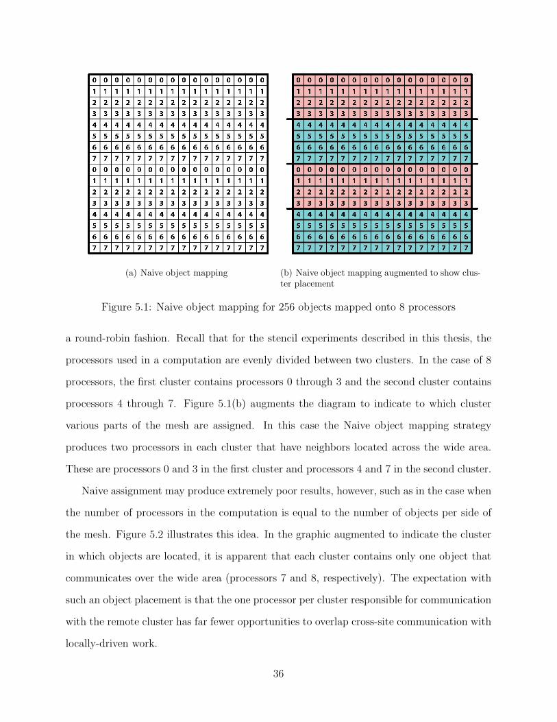
(a) Naive object mapping (b) Naive object mapping augmented to show clus-ter placement
Figure 5.1: Naive object mapping for 256 objects mapped onto 8 processors
a round-robin fashion. Recall that for the stencil experiments described in this thesis, the
processors used in a computation are evenly divided between two clusters. In the case of 8
processors, the first cluster contains processors 0 through 3 and the second cluster contains
processors 4 through 7. Figure 5.1(b) augments the diagram to indicate to which cluster
various parts of the mesh are assigned. In this case the Naive object mapping strategy
produces two processors in each cluster that have neighbors located across the wide area.
These are processors 0 and 3 in the first cluster and processors 4 and 7 in the second cluster.
Naive assignment may produce extremely poor results, however, such as in the case when
the number of processors in the computation is equal to the number of objects per side of
the mesh. Figure 5.2 illustrates this idea. In the graphic augmented to indicate the cluster
in which objects are located, it is apparent that each cluster contains only one object that
communicates over the wide area (processors 7 and 8, respectively). The expectation with
such an object placement is that the one processor per cluster responsible for communication
with the remote cluster has far fewer opportunities to overlap cross-site communication with
locally-driven work.
36

(a) Naive object mapping (b) Naive object mapping augmented to show thatonly one border processor exists per cluster
Figure 5.2: Naive object mapping for 256 objects mapped onto 16 processors
5.2 Block Mapping
A more sophisticated way to map objects to processors in the computation is to use a
configuration in which objects are arranged in square or rectangular blocks. Recall that a
fundamental idea for achieving good latency tolerance with the Charm++ runtime system
in a Grid computing environment is that each processor should have a relatively small
number of objects that communicate across cluster boundaries and a relatively large number
of objects that communicate with only local neighbors. Thus an ideal object mapping
strategy would arrange objects such that the “border” objects, those that communicate
across cluster boundaries, are spread as evenly as possible across the largest number of
processors per cluster possible. The expectation here is that this strategy should provide the
greatest number of opportunities to overlap high-latency remote communication with local
communication. Figure 5.3 shows an object mapping strategy, referred to as Block mapping
in this thesis, that reflects such a configuration. In the figure, 256 objects (16x16) are divided
evenly across two clusters. Within each cluster, 128 objects are divided evenly among the 8
37

Figure 5.3: Block object mapping for 256 objects mapped onto 8 processors
processors, resulting in 16 objects per processor. As shown in the figure, these are arranged
in a rectangular pattern in which 2 objects communicate across the cluster boundary and
14 objects communicate only with neighboring objects within the local cluster.
It should be noted that in a stencil decomposition problem that is not running in a
Grid environment, an optimal object mapping strategy is to arrange objects into as near
square blocks as possible. Such a configuration results in the largest amount of inter-object
communication as possible staying within each processor, and minimizes as much as possible
the amount of inter-processor communication. A square mapping strategy, however, would
not directly map objects such that the border objects were as evenly spread across all
processors within a cluster. It is possible to slightly modify the square object mapping
strategy to allow an even distribution of border objects, however. First, all objects except
the border objects on each cluster are arranged into blocks that are as close to square as
possible. Next, the border objects on each cluster are spread evenly among the processors
within the cluster. The difficulty with this strategy is that for the simple stencil benchmark
considered in this thesis, each processor must have exactly the same number of objects in
order to avoid a noticeable performance degradation due to overloading some processors and
38

underloading other processors. The Block mapping strategy used in this thesis is a much
simpler approximation that ensures that each processor has an equal number of objects and
that the border objects are evenly distributed.
The graphs described in the previous chapter in Figure 4.4 and Figure 4.5 are for Naive
object mapping. Figure 5.4 and Figure 5.5 show similar graphs for Block object mapping
for the 2048x2048 and 8192x8192 mesh sizes respectively. The overall trends in these graphs
are similar to the Naive mapping graphs, however some differences do become apparent after
careful comparison. For example, for the 2048x2048 mesh on 8 processors with 64 objects
(Figures 4.4(a) and 5.4(a)), one can clearly see that although the lines for Naive and Block
mapping appear to be fairly similar through 8 milliseconds of latency, after this point the
Naive results seem to lose performance much more rapidly than the Block results. This is an
important observation because it reinforces the notion that improved latency tolerance can
be achieved by placing a relatively small number of border objects along with a relatively
large number of local-only objects on each processor. On the same graph, the results for
1024 objects are overall much worse for Naive mapping (approximately 40 milliseconds per
step) than for Block mapping (approximately 30 milliseconds per step). The graphs for
larger numbers of processors show similar results, particularly when comparing the results
between Naive and Block mappings for the largest number of objects per processor. This
also makes sense because the Block mapping reduces the overall volume of communication
necessary by mapping larger numbers of neighboring objects onto the same processor.
Similar results are also present in the graphs for the 8192x8192 mesh size. Here again, the
results for Block mapping show improved latency masking capability over Naive mapping,
such as in the case for 16 processors and 64 objects (Figures 4.5(b) and 5.5(b)) or in the
case for 64 processors and 256 objects (Figures 4.5(d) and 5.5(d)). For these graphs, the
larger mesh size makes a more pronounced impact on the differences between Naive and
Block object mappings than was observable before. Finally, as before, the results for the
largest number of objects per processor clearly show that Block mapping offers much better
39
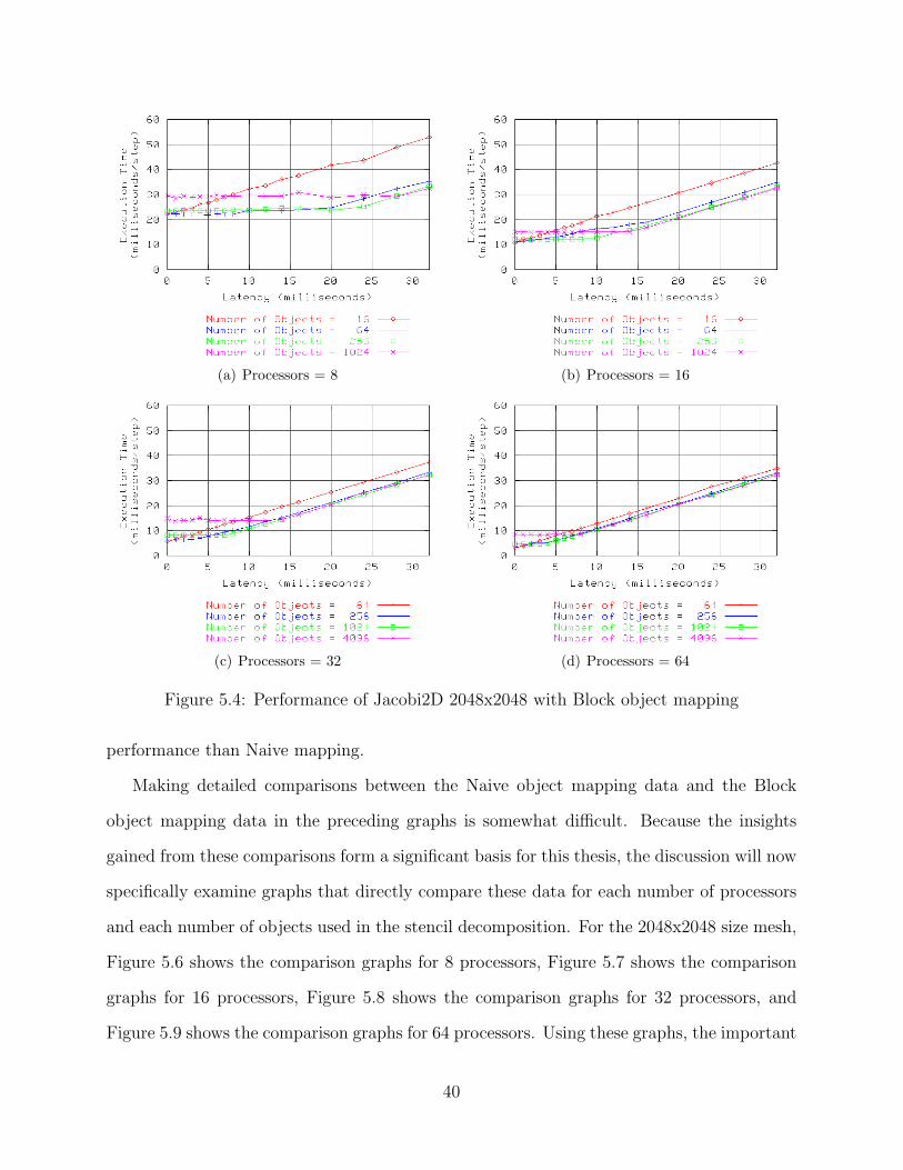
(a) Processors = 8 (b) Processors = 16
(c) Processors = 32 (d) Processors = 64
Figure 5.4: Performance of Jacobi2D 2048x2048 with Block object mapping
performance than Naive mapping.
Making detailed comparisons between the Naive object mapping data and the Block
object mapping data in the preceding graphs is somewhat difficult. Because the insights
gained from these comparisons form a significant basis for this thesis, the discussion will now
specifically examine graphs that directly compare these data for each number of processors
and each number of objects used in the stencil decomposition. For the 2048x2048 size mesh,
Figure 5.6 shows the comparison graphs for 8 processors, Figure 5.7 shows the comparison
graphs for 16 processors, Figure 5.8 shows the comparison graphs for 32 processors, and
Figure 5.9 shows the comparison graphs for 64 processors. Using these graphs, the important
40
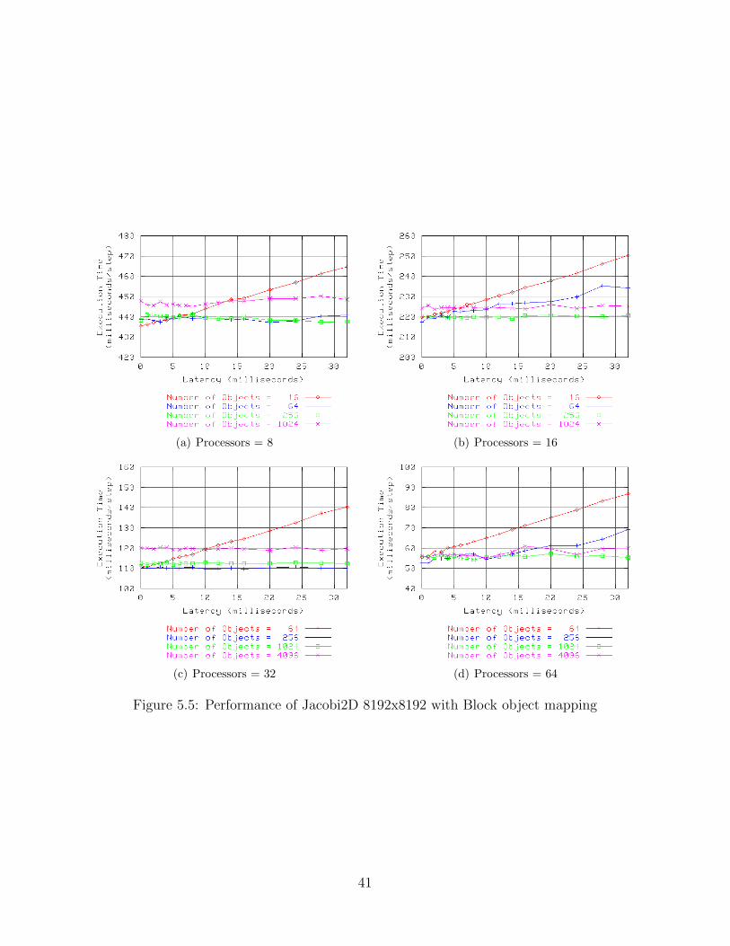
(a) Processors = 8 (b) Processors = 16
(c) Processors = 32 (d) Processors = 64
Figure 5.5: Performance of Jacobi2D 8192x8192 with Block object mapping
41

characteristics of the experiments become quite apparent. For the graphs for the least
number of objects per processor (Figures 5.6(a), 5.7(a), 5.8(a), and 5.9(a)), the trend in the
data clearly indicates that there is little or no difference between Naive and Block mapping.
The data for 8 processors and 16 objects shows the most difference with Block mapping being
approximately 2 milliseconds per timestep better than Naive mapping at some points. The
data for 16 processors and 16 objects, 32 processors and 64 objects, and 64 processors and
64 objects show nearly identical results for the two mapping strategies. As described above,
this makes sense because in these cases there is only one or two objects per processor, so the
mapping strategy is largely irrelevant because either strategy produces a similar distribution
of objects onto processors. For the graphs for the largest number of objects per processor
(Figures 5.6(d), 5.7(d), 5.8(d), and 5.9(d)), the trend in the data clearly indicates that Block
mapping provides superior performance in all cases. For the case of 8 processors, the Block
mapping results are consistently better than the results for Naive mapping, however it is
apparent at 32 milliseconds of latency that the Block mapping line is beginning to slope
upwards. For 16, 32, and 64 processors, Block mapping provides better performance than
Naive mapping, as much as 5 to 6 milliseconds per application timestep. Again, after the
latency matches the per-step time for the application, each line begins to slope upwards
indicating that the effects of latency are not being completely masked.
The most interesting graphs are the ones corresponding to the middle number of objects
for each number of processors (Figures 5.6(b) and 5.6(c), 5.7(b) and 5.7(c), 5.8(b) and 5.8(c),
and 5.9(b) and 5.9(c)) because these graphs represent a sort of “middle ground” between
having far too few objects to expect any sort of latency masking and so many objects that
the effects of reduced inter-processor communications even within a single cluster have a
positive impact on performance. That is, in these middle ground graphs, it is possible to
get some idea of the usefulness of careful object placement on the latency tolerance of the
stencil problem. For example, for the case of 8 processors and 64 objects (Figure 5.6(b)),
the differences in latency tolerance that were hinted at before in Figures 4.4 and 5.4 are
42

now quite apparent between 8 and 32 milliseconds of latency. This graph shows the largest
improvement in performance due to Block object mapping, and this large improvement may
actually be due to using only 8 processors (4 processors in each cluster) which is probably
the least number of processors that would realistically be used for running a realistic parallel
application. Other graphs in the middle regions show a more subtle difference due to object
mapping, such as Figure 5.7(b) between 4 and 14 milliseconds of latency, Figure 5.8(b)
between 12 and 32 milliseconds of latency, Figure 5.9(b) between 4 and 16 milliseconds of
latency, and Figure 5.9(c) between 12 and 32 milliseconds of latency. The differences in
these graphs are much less obvious, on the order of perhaps 500 microseconds per timestep
performance improvement for Block mapping over Naive mapping, but they are consistently
present. Further, although it is possible to find situations in the graphs where Naive mapping
produces slightly better performance than Block mapping, for example in Figure 5.7(c)
between 10 and 16 milliseconds of latency, these situations occur much less frequently, and
when they do appear they last for only two or three data points at a time. Overall, the
results in these graphs suggest that Block mapping does in fact offer enhanced latency
masking benefits over Naive mapping, due to careful arrangement of objects such that each
processor has a relatively small number of border objects and a relatively large number of
locally-driven objects.
For the 8192x8192 size mesh, Figure 5.10 shows the comparison graphs for 8 processors,
Figure 5.11 shows the comparison graphs for 16 processors, Figure 5.12 shows the comparison
graphs for 32 processors, and Figure 5.13 shows the comparison graphs for 64 processors.
Overall, these results closely match those from the 2048x2048 mesh size, although the larger
size problem helps to highlight the differences in performance between Naive and Block
mapping. Like before, the results for the least number of objects per processor (Figures
5.10(a), 5.11(a), 5.12(a), and 5.13(a)) produce similar results for either object mapping
strategy, and any differences that do show up between the two strategies in these graphs are
much less pronounced than the differences in the other graphs for this problem size. This
43

(a) Processors = 8, Number of Objects = 16 (b) Processors = 8, Number of Objects = 64
(c) Processors = 8, Number of Objects = 256 (d) Processors = 8, Number of Objects = 1024
Figure 5.6: Performance comparison of Jacobi2D 2048x2048 Naive object mapping vs. Blockobject mapping (8 processors)
44
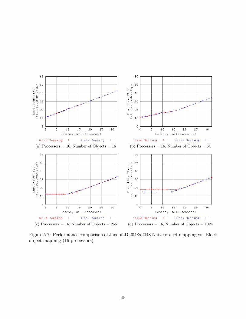
(a) Processors = 16, Number of Objects = 16 (b) Processors = 16, Number of Objects = 64
(c) Processors = 16, Number of Objects = 256 (d) Processors = 16, Number of Objects = 1024
Figure 5.7: Performance comparison of Jacobi2D 2048x2048 Naive object mapping vs. Blockobject mapping (16 processors)
45

(a) Processors = 32, Number of Objects = 64 (b) Processors = 32, Number of Objects = 256
(c) Processors = 32, Number of Objects = 1024 (d) Processors = 32, Number of Objects = 4096
Figure 5.8: Performance comparison of Jacobi2D 2048x2048 Naive object mapping vs. Blockobject mapping (32 processors)
46

(a) Processors = 64, Number of Objects = 64 (b) Processors = 64, Number of Objects = 256
(c) Processors = 64, Number of Objects = 1024 (d) Processors = 64, Number of Objects = 4096
Figure 5.9: Performance comparison of Jacobi2D 2048x2048 Naive object mapping vs. Blockobject mapping (64 processors)
47
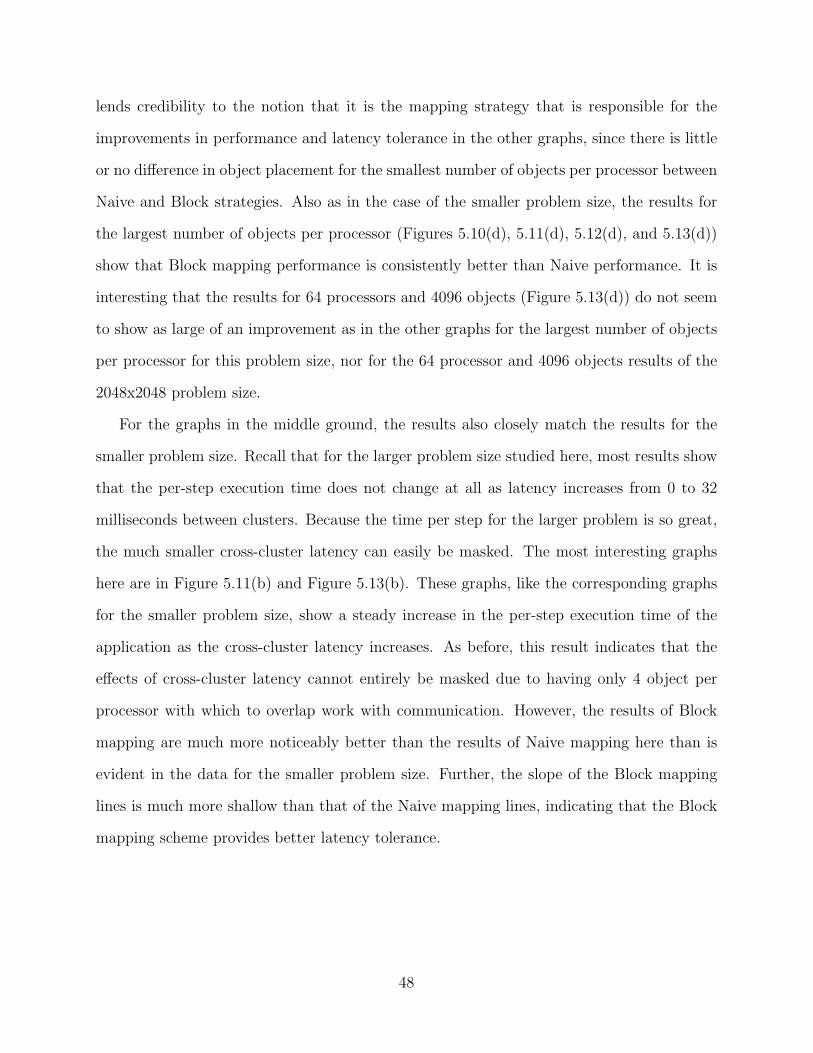
lends credibility to the notion that it is the mapping strategy that is responsible for the
improvements in performance and latency tolerance in the other graphs, since there is little
or no difference in object placement for the smallest number of objects per processor between
Naive and Block strategies. Also as in the case of the smaller problem size, the results for
the largest number of objects per processor (Figures 5.10(d), 5.11(d), 5.12(d), and 5.13(d))
show that Block mapping performance is consistently better than Naive performance. It is
interesting that the results for 64 processors and 4096 objects (Figure 5.13(d)) do not seem
to show as large of an improvement as in the other graphs for the largest number of objects
per processor for this problem size, nor for the 64 processor and 4096 objects results of the
2048x2048 problem size.
For the graphs in the middle ground, the results also closely match the results for the
smaller problem size. Recall that for the larger problem size studied here, most results show
that the per-step execution time does not change at all as latency increases from 0 to 32
milliseconds between clusters. Because the time per step for the larger problem is so great,
the much smaller cross-cluster latency can easily be masked. The most interesting graphs
here are in Figure 5.11(b) and Figure 5.13(b). These graphs, like the corresponding graphs
for the smaller problem size, show a steady increase in the per-step execution time of the
application as the cross-cluster latency increases. As before, this result indicates that the
effects of cross-cluster latency cannot entirely be masked due to having only 4 object per
processor with which to overlap work with communication. However, the results of Block
mapping are much more noticeably better than the results of Naive mapping here than is
evident in the data for the smaller problem size. Further, the slope of the Block mapping
lines is much more shallow than that of the Naive mapping lines, indicating that the Block
mapping scheme provides better latency tolerance.
48
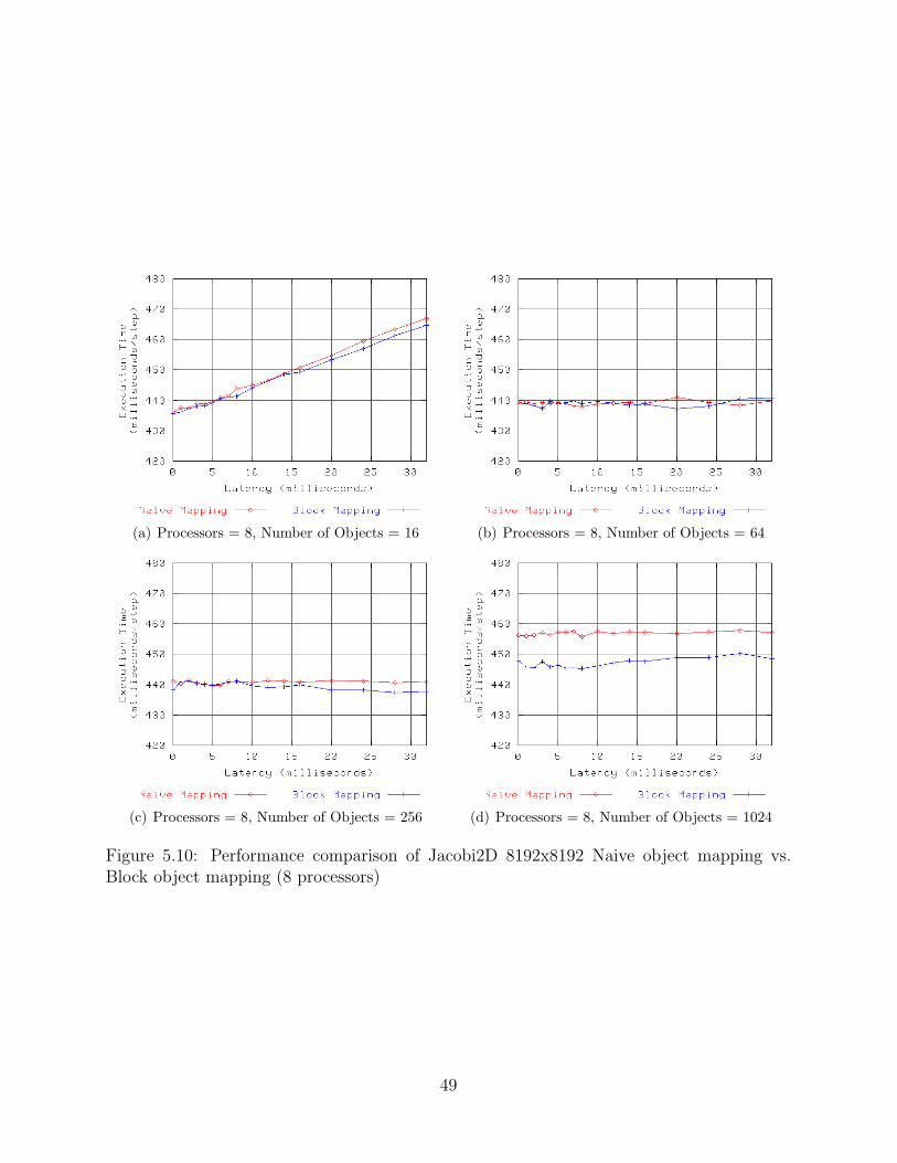
(a) Processors = 8, Number of Objects = 16 (b) Processors = 8, Number of Objects = 64
(c) Processors = 8, Number of Objects = 256 (d) Processors = 8, Number of Objects = 1024
Figure 5.10: Performance comparison of Jacobi2D 8192x8192 Naive object mapping vs.Block object mapping (8 processors)
49

(a) Processors = 16, Number of Objects = 16 (b) Processors = 16, Number of Objects = 64
(c) Processors = 16, Number of Objects = 256 (d) Processors = 16, Number of Objects = 1024
Figure 5.11: Performance comparison of Jacobi2D 8192x8192 Naive object mapping vs.Block object mapping (16 processors)
50

(a) Processors = 32, Number of Objects = 64 (b) Processors = 32, Number of Objects = 256
(c) Processors = 32, Number of Objects = 1024 (d) Processors = 32, Number of Objects = 4096
Figure 5.12: Performance comparison of Jacobi2D 8192x8192 Naive object mapping vs.Block object mapping (32 processors)
51
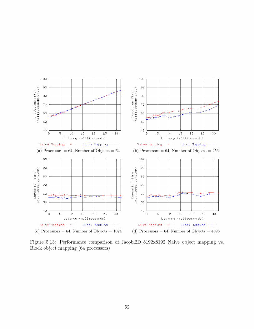
(a) Processors = 64, Number of Objects = 64 (b) Processors = 64, Number of Objects = 256
(c) Processors = 64, Number of Objects = 1024 (d) Processors = 64, Number of Objects = 4096
Figure 5.13: Performance comparison of Jacobi2D 8192x8192 Naive object mapping vs.Block object mapping (64 processors)
52

5.3 Summary
This chapter has examined the effects that the strategy for mapping objects to processors has
on the performance of the five-point stencil benchmark when running in a Grid environment.
The results of experiments in the chapter suggest that a block-oriented object mapping, in
which each processor contains a relatively small number of border objects that communicate
with neighbors across cluster boundaries and a relatively large number of objects that are
driven by neighbors within the local cluster, provides the Charm++ runtime system with
the best opportunities to mask the effects of cross-cluster latency. The object prioritization
technique presented in Chapter 6 assume such a configuration of objects on each processor.
The importance of efficiently allocating blocks of work to computational resources has
been extensively studied in systems such as KeLP [5]. Manually mapping objects to proces-
sors is straightforward for simple benchmarks like Jacobi2D. For more complex applications,
the manual mapping of objects becomes increasingly difficult. The complexity continues to
increase when applications are deployed into Grid environments because of the non-uniform
structure of inter-processor communication (i.e., communication between one pair of pro-
cessors may be several orders of magnitude faster or slower than communication between
another pair) and because of the pervasive heterogeneity often found in these environments.
This is, in fact, the main conclusion that can be drawn from comparing the simple Naive
mapping strategy, which has the potential to create unintended performance bottlenecks
when used in a Grid environment, to the more complicated Block mapping strategy in this
chapter. Further, if an efficient manual mapping of objects to processors is able to be found,
this mapping may tend to encapsulate specific characteristics of the Grid environment into
the application software. This is usually undesirable because it makes the application less
portable to other environments. Automated systems, such as KeLP, are thus very desirable.
To that end, the discussion in Chapter 7 presents a set of techniques that dynamically map
objects to processors while taking the Grid environment into consideration.
53

Chapter 6
Object Prioritization
Chapter 4 describes a technique for efficiently executing tightly-coupled parallel applications
in Grid computing environments by using message-driven objects within the runtime system
layer to mask the effects of cross-cluster latency. Using this technique, it is possible to deploy
tightly-coupled applications in many realistic Grid environments and achieve performance
that is on par with what the application achieves when running within a single cluster. This
technique is the fundamental architectural contribution of this thesis. As demonstrated in
Chapter 5, the technique produces the best results when each processor in a computation
contains a favorable mix of a relatively small number of border objects and a relatively large
number of local-only objects. Such a mix of objects provides each processor with an equal
chance of finding locally-driven work to use for masking latency.
This chapter presents an optimization technique in which portions of a tightly-coupled
application are prioritized to improve performance in Grid environments. This technique
is effective in situations where the effects of latency cannot be entirely masked due to an
insufficient amount of locally-driven work. In these situations, application performance
begins to deviate from the single-cluster performance, and the technique presented in this
chapter may be useful for getting the best possible performance in a Grid environment.
6.1 Object Prioritization Technique
An important insight about the latency masking capability of the Charm++ runtime system
is that it works best when the execution in objects is coordinated such that border objects
54
are driven earlier than local-only objects during each timestep. That is to say, if a mechanism
existed for prioritizing the execution of the border objects on each processor such that these
objects were executed in preference to the local-only objects, it should be possible to overlap
a greater amount of the otherwise-wasted time with useful work. This is in contrast to simply
selecting the next available object without regard to whether the object is a border object
or a local-only object. With this simplistic scheduling scheme, an unfortunate scheduling
of the objects during a timestep might “waste” the locally-driven work by executing all or
most of it earlier in the timestep than the work in border objects. It should be clear that
this technique assumes a favorable mapping of objects to processors in each cluster, with
each processor holding a relatively small number of border objects and a larger number
of local-only objects. Such a favorable mapping gives each processor a roughly equivalent
opportunity to proceed through each application timestep at the same pace. Without such
a mapping, prioritizing the execution of border objects on some subset of the processors in a
cluster is likely to simply cause these processors to progress faster than processors that are
dominated by local-only objects, resulting in the processors that move faster through the
computation being forced to wait on the processors that make slower forward progress.
Section 6.2 describes details of the optimization’s implementation in terms of the Charm++
runtime system. Section 6.3 evaluates the performance benefits of this optimization in terms
of the five-point stencil decomposition benchmark examined in the previous chapters. Sec-
tion 6.4 enumerates some of the limitations of the technique.
6.2 Implementation Details
The technique described in the previous section involves prioritizing the execution of each
processor’s border objects ahead of its local-only objects. The Charm++ runtime system,
however, does not directly associate priorities with objects. Instead, object execution simply
follows the scheduling of incoming messages on each processor. Thus, in the Charm++
55
message-driven execution model, prioritizing the messages destined for the border objects
on each processor has the same effect as prioritizing the border objects themselves.
Execution within Charm++ objects is carried out inside entry methods. The execution
of an entry method proceeds uninterrupted until the code path within the entry method
is exhausted. Typically, the code within an entry method generates one or more messages
which are used to drive further execution in either the same object or another object in
the computation. When execution in an entry method ends, the next waiting message is
dequeued from the Charm++ Scheduler’s message queue and this message triggers execution
within one of the waiting objects on the processor. By default, the Charm++ Scheduler
processes messages in FIFO order, although facilities exist for message prioritization using
either integer or arbitrary-length bitvector priorities. To use message prioritization, the
application tags each outgoing message with a priority. On the receiving processor, the
Charm++ Scheduler dequeues messages in priority order. Messages of equal priority are
still processed in FIFO order relative to one another.
Directly using message priorities to implement the technique of border object prioritiza-
tion presents at least two difficulties. First, the integer or bitvector priority associated with
each message must be sent along with the message data, and this increases the overhead
for each message when prioritization is in use. Because message priorities are not useful to
all Charm++ programs, the Charm++ message structure is designed to make the priority
fields optional. This means that using message priorities internally in the Charm++ kernel
would have to first determine whether the user-level application was using message priorities
and turn the feature on if it was not actively being used. This is further complicated if the
user-level application is using message priorities itself because the message priorities used
inside the Charm++ kernel would have to coexist with the user-level priorities.
The second, and more challenging, difficulty in directly using message priorities to im-
plement the technique of border object prioritization is that each processor in the compu-
tation must know which objects are border objects and which objects are local-only objects
56
throughout the entire computation. Figure 6.1 illustrates this concept. The figure shows
three processors (PE0, PE1, and PE2) in two clusters separated by a wide-area connection.
PE0 and PE1 are located in the first cluster and PE2 is located in the second cluster. Six
objects are used in the figure: Objects A and B are located on PE0; Objects C, D, and E
are located on PE1; and Object F is located on PE2. Five messages are shown being sent
between objects. Based on these messages, Objects A, B, D, and E are local-only objects
because they communicate only with objects in the same cluster while Objects C and F
are border objects because they communicate with objects in other clusters. This means
that to implement the border object prioritization technique, execution on PE1 should pri-
oritize Object C over Objects D and E. Using message priorities to drive Object C with
higher priority requires the message senders to have distributed knowledge of the border
and local-only objects on PE1. For example, Object A on PE0 must know that Object E
on PE1 is a local-only object when it sends Message 1. Or, Object B on PE0 must know
that Object C on PE1 is a border object and that Object D on PE1 is a local-only object
so that it can prioritize messages to these objects accordingly. In practice, maintaining a
consistent view of this kind of distributed state is a traditionally challenging problem in
distributed systems. The Charm++ kernel already keeps a distributed database of the map-
ping of objects to processors in a computation, called the Location Manager database. This
database is updated when objects migrate to new processors, such as during load balancing,
so that messages can be sent to the correct processors. One possibility for distributing the
knowledge of border and local-only objects on each processor is to use the Location Manager
database. However, to avoid the challenging problem of keeping a consistent state for this
database on each processor, the Location Manager database is not guaranteed to contain
up-to-date information on each processor. That is, if an object migrates from one processor
to another, the Location Manager database on some processors may indicate that the object
resides on the old processor while the Location Manager database on other processors may
indicate that the object resides on the new processor. For message sends, this limitation is
57

Figure 6.1: Example of border object prioritization
dealt with by having each processor agree to forward messages to the correct destination for
objects that have recently migrated away from the processor. Eventually when the Location
Manager database on each processor is updated to reflect the correct state, this forwarding
is no longer necessary. For implementing border object prioritization, imprecise information
may be sufficient; if some messages are incorrectly prioritized, it is unlikely to matter to the
overall application performance as long as correct knowledge of border and local-only objects
eventually gets distributed to each processor. However, due to the limitations of the Loca-
tion Manager database as well as the challenges to using message priorities outlined above,
this scheme is perhaps not the optimal way to implement the border object prioritization
technique.
Recall the discussion above about how object execution is scheduled by the Charm++
kernel by retrieving messages from a Scheduler Queue on each processor. An important
insight is that not only can each processor in a computation deduce knowledge about which
58

of its objects are border objects and which of its objects are local-only objects by observing
the destination processor for each outgoing message, but also that each processor has its
own Scheduler that can adjust its behavior according to this knowledge. To this end, the
border object prioritization technique can be implemented by introducing a second queue
on each processor which is serviced at higher priority than the existing Scheduler Queue. By
placing messages destined for border objects into this Grid Queue as they are received and
then servicing the Grid Queue with higher priority, the border objects on each processor
will be driven before the local-only objects. An advantage of implementing the border
object prioritization technique using a separate Grid Queue is that any user-level message
priorities will continue to be honored as a second-level criteria for the next message selected
for dispatch by the Scheduler. That is, messages in the Grid Queue will be serviced in order
of their user-level message priorities, and these messages will all be serviced at a higher
priority than the messages in the Scheduler Queue which are also serviced in order of their
user-level message priorities.
Implementing the border object prioritization technique involves modifying the Charm++
kernel’s code path for both message sends and message receives. For the send code, the ob-
jective is to identify which objects send messages to objects on a remote cluster and to record
these sending objects in a table of border objects on the current processor. During a message
send, the source object and destination object are both known. The Charm++ kernel uses
the destination object identification to find the destination processor using the Location
Manager as described above. The modified code path further looks up the cluster for the
sending processor and the cluster for the destination processor. These processor-to-cluster
mappings are determined during the Charm++ startup process either by being specified by
the user or by being discovered automatically via a latency probing process and then the
mapping information is distributed to each processor in the computation. If the source and
destination clusters differ, the sending object is a border object. In this case, the sending
object’s identification, an integer group ID and three integer index values used to identify
59

the object internally to the Charm++ kernel, is recorded in a table of border objects on the
processor.
On the receive side, the Charm++ header of each incoming message is examined to
determine its destination object identification. The border object table is then consulted to
determine whether the destination object is a border object. If it is, the incoming message is
enqueued into the Grid Queue, otherwise it is enqueued into the normal-priority Scheduler
Queue. When the Charm++ Scheduler looks for the next waiting message, it first examines
the Grid Queue. Any message in this queue is dequeued in order of any user-specified
message priority. If the Grid Queue is empty, the Scheduler Queue is examined in a similar
fashion and any waiting messages are dequeued. In theory, it is possible that local-only
objects could suffer from starvation in this implementation if a constant stream of incoming
messages are destined for border objects. To prevent this, after a fixed number of objects
are dequeued from the Grid Queue, a forced check of the Scheduler Queue is made.
6.3 Performance Evaluation
The first step in evaluating the performance impact of object prioritization is understanding
when the optimization can improve performance. The configurations for the experiments in
Chapter 4 demonstrate the effects of increasing the number of objects per physical processor
from one or two objects per processor, such as in the example of Figure 5.6(a), to over
a hundred objects per processor, such as in the example of Figure 5.6(d). Because the
object prioritization technique relies on being able to favor the execution on some objects
(border objects) over the execution of others (local-only objects), configurations with very
small numbers of objects per processor cannot see improvements with the optimization
due to the fact that the Charm++ Scheduler has no choice regarding the next object to
schedule for execution on a processor. On the other hand, configurations in which the
largest number of objects per processor are used, such as in Figure 5.6(d), often remain flat
60

for the entire range of latencies shown on the graphs, meaning that the effects of latency
are being entirely masked. That is to say, the per-step execution time for a latency of
0 milliseconds, representing the “base” performance of the application for that particular
number of processors and number of objects, includes enough overall work that latency has
no effect on the application for the range of latencies studied. The object prioritization
technique also can have little or no effect in these regions of the graphs because there is
overall enough work to mask latency; rearranging the order in which the work is performed
in these cases cannot improve performance. Further, situations where the flat region ends
and the graph transitions into a region where the per-step execution time increases linearly
with latency, such as in Figure 5.7(d), also represent situations where object prioritization
can have little or no effect because the application’s performance in these regions is totally
dominated by latency. In these cases, not enough overall work is available on each processor
to mask the increasing latency, so arranging the border object work to occur early in the
timestep relative to the locally-driven work can show little improvement in performance.
Any small performance improvement in these circumstances would be dwarfed by the large
decrease in performance due to idle time on each processor.
The circumstances where object prioritization can show an improvement in performance
are situations where the application can almost, but not quite, mask the effects of latency. In
these circumstances, the application’s per-step time increases with latency, but this increase
is less than linear. Examples of these circumstances are shown in Figures 5.6(b), 5.7(b), and
to some extent 5.8(b) for the 2048x2048 problem size, and in Figures 5.11(b) and 5.13(b)
for the 8192x8192 problem size. In these configurations, a small number of objects, four or
eight, exist per processor. Of these four or eight objects, one or two are border objects and
the remainder are local-only objects. It is in these cases where prioritizing the execution of
the border objects can slightly improve performance because the prioritization causes the
border objects to be driven early in the timestep relative to the local-only objects, allowing
more chances to mask the high cross-cluster latency as described above. The discussion in
61
the following paragraphs examines the data for the graphs outlined above.
The first dataset in which the effects of object prioritization can be seen is from Fig-
ure 5.6(b). Because the effects of object prioritization are very subtle for this small problem
size, the data are shown in tabular form in Table 6.1. For this problem configuration, the
geometry of the Naive mapping results in only one processor per cluster being arranged on
the border. In the first cluster, Processor 3 contains all objects that communicate across the
cluster boundary; in the second cluster, Processor 4 contains all border objects. Because the
border objects in each cluster are arranged onto a single processor, and because this proces-
sor contains no objects other than border objects, the expectation here is that the object
prioritization technique should show no appreciable change in performance. The data in the
Table reflect this notion, with the results for Naive execution and Naive with Prioritization
closely matching each other. The geometry for the Block mapping involves each of the four
processors per cluster containing two border objects mixed with six local-only objects. This
is an ideal circumstance for the object prioritization technique to improve performance by
driving the border object execution favorably relative to the local-only objects. The data for
0 millisecond latency separating the clusters gives the basic per-step execution time of the
application, and this value is near 22 milliseconds per step for both the Block case and the
Block with Prioritization case. This per-step time remains consistent through 8 milliseconds
of cross-cluster latency. After 8 milliseconds of cross-cluster latency, however, the per-step
execution time for the Block case enters another apparently flat region, increasing to approx-
imately 23.7 milliseconds within the region between 10 and 16 milliseconds of cross-cluster
latency. That is, the increase from 8 to 10 milliseconds of cross-cluster latency causes almost,
but not quite, a corresponding 2 millisecond increase in the per-step execution time of the
application followed by another region of latency tolerance. The Block with Prioritization
case, however, shows different results in this same region. The per-step execution time of the
Block with Prioritization case appears to stay flat, near 22 milliseconds per step, through
10 and 12 milliseconds of cross-site latency. At 14 milliseconds, the 2 millisecond increase
62

Naive with Block withLatency Naive Prioritization Block Prioritization
0 21.94 21.97 21.93 21.901 22.42 21.91 22.23 21.872 22.36 22.28 21.95 21.663 22.11 22.09 22.07 21.904 22.17 22.05 21.98 21.925 22.11 22.09 21.90 21.996 22.46 22.09 22.14 21.867 22.86 22.87 22.01 21.828 22.43 22.43 21.94 21.8510 24.51 24.68 23.71 21.5112 24.89 24.89 23.70 21.9214 25.26 25.54 23.41 22.8516 25.85 26.03 23.84 23.5120 29.09 28.93 24.86 24.5624 30.16 30.33 28.35 28.1728 33.56 33.76 32.23 32.1432 35.72 35.88 35.31 36.35
Table 6.1: Performance of Jacobi2D 2048x2048 object prioritization with 8 processors and64 objects
in cross-site latency appears to cause only an approximately 1 millisecond increase in the
per-step application execution time. This is similar to the next step between 14 and 16 mil-
liseconds of latency between clusters, where the per-step execution time increases again by
approximately only 1 millisecond. By the time the 16 millisecond point is reached, however,
the performance of the Block with Prioritization case nearly matches the performance of the
non-prioritized Block case. The next step in cross-site latency, from 16 to 20 milliseconds,
sees both cases increasing their per-step execution times by approximately 1 millisecond for
the 4 millisecond increase in latency. The results after this point, however, enter a region
where the effects of latency no longer can be masked at all. Each 4 millisecond increase in
cross-site latency increases the per-step execution time of the application by a corresponding
4 milliseconds.
The results in Table 6.1 suggest that the object prioritization technique may have an im-
pact on application performance. Unfortunately, the differences in the observed application
63

performance are quite subtle for this small problem size. This is not entirely unexpected,
however. Consider the difference between unprioritized Naive and Block mapping strategies
in the same problem size. Entirely rearranging the mapping of objects to processors pro-
duces at most an approximately 4 millisecond difference in performance at 20 milliseconds
of latency. The expectation, therefore, is that any benefits of the object prioritization tech-
nique, where only the execution order of objects already mapped to a processor is changed,
would be more subtle in comparison.
Table 6.2 shows the results for 16 processors and 64 objects. Because the effects of prior-
itization are particularly well observable here, Figure 6.2 echoes the Table data graphically.
In this configuration, the Naive mapping scheme results in a situation where every object
in both halves of the computation communicates with a neighbor on the remote cluster.
Similar to the previous case, the expectation here is that prioritization cannot improve the
performance of the Naive case because every object becomes prioritized and is thus serviced
at the same priority as every other object. Indeed, the results in the Naive with Prioritiza-
tion column closely match those in the Naive column. For this problem configuration, the
Block mapping strategy results in an object layout where each of the eight processors in both
clusters contain four objects, with one of these objects being a border object and three being
local-only objects. The base per-step time of the application at 0 milliseconds of latency is
approximately 11 milliseconds, and this is reflected in both the Block results and the Block
with Prioritization results. As the cross-cluster latency increases from 0 to 1 milliseconds,
both results tolerate the latency increase somewhat by increasing the per-step execution time
by approximately 0.25 milliseconds. The latency increase from 1 to 2 milliseconds causes
approximately a 0.50 millisecond increase in execution time for both Block and Block with
Prioritization cases. As cross-cluster latencies increase in 1 millisecond increments from 2
milliseconds to 7 milliseconds, the per-step execution time continues the trend of increasing
in a latency-tolerant fashion in the neighborhood of 0.25 to 0.50 milliseconds per increment
of cross-site latency. The interesting points in the data appear at 8 and 10 milliseconds of
64

cross-cluster latency. During the transition from 7 to 8 milliseconds of latency, the Block
performance increases from 14.23 to 15.36 milliseconds per timestep, an increase of approx-
imately 1 millisecond. The Block with Prioritization performance, however, increases from
only 14.22 to 14.55 during this same region, suggesting that the prioritization technique
allows better latency tolerance at this point when the non-prioritized case begins to lose its
ability to mask latency. Both configurations have the same number of objects with which
to work, but the better performance for the Block with Prioritization case seems to indicate
that it is arranging this work in such a way as to make the best use of its locally-driven
objects to mask the effects of cross-site latency. As the cross-cluster latency increases from 8
to 10 milliseconds, the Block case execution time increases by 1 millisecond per step. During
this same period, however, the Block with Prioritization case increases by 1.3 milliseconds
per step. This makes sense: in situations where unprioritized execution begins to show signs
of decreased latency tolerance, prioritized execution retains its ability to “hang on” to better
performance by rearranging the order of object execution in order to make the best use of
locally-driven work. However after some amount of this reordering process, the ability of the
prioritization technique breaks down faster as latency increases due to the fact that cross-
cluster messages take longer to arrive onto the processor. This means that locally-driven
work has a higher chance of being executed earlier in a timestep even though prioritization
is in use, since the Charm++ Scheduler will execute lower-priority locally-driven objects
rather than letting the processor sit idle waiting for messages from the remote cluster to
arrive. Thus, the prioritized execution case will begin to “catch up” to the unprioritized
execution case as both cases approach the limits of effective latency tolerance. This happens
in the data from the table by the time both cases reach the 12 millisecond latency point. By
the 16 milliseconds of cross-site latency point, both cases are clearly dominated by latency
and begin to increase linearly with latency.
Table 6.3 shows the results for 32 processors and 256 objects. The geometry of this
problem is similar to the 16 processor and 64 object configuration, and as in the previous
65

Naive with Block withLatency Naive Prioritization Block Prioritization
0 11.02 11.06 10.98 11.011 11.40 11.35 11.25 11.222 11.91 11.69 11.73 11.713 12.50 12.24 12.02 12.054 12.90 12.97 12.61 12.445 13.68 13.21 12.96 13.066 13.94 13.61 13.70 13.527 15.34 15.41 14.23 14.228 15.94 15.74 15.36 14.5510 16.83 16.92 16.34 15.8712 17.40 16.89 16.83 16.8714 17.99 17.96 17.96 17.9316 18.96 18.97 18.92 18.8820 23.00 22.84 22.80 22.7724 26.83 26.79 26.78 26.7928 30.79 30.77 30.78 30.7732 34.79 34.79 34.78 34.79
Table 6.2: Performance of Jacobi2D 2048x2048 object prioritization with 16 processors and64 objects
Figure 6.2: Performance comparison of Jacobi2D 2048x2048 object prioritization with 16processors and 64 objects
66
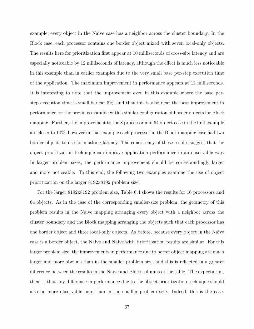
example, every object in the Naive case has a neighbor across the cluster boundary. In the
Block case, each processor contains one border object mixed with seven local-only objects.
The results here for prioritization first appear at 10 milliseconds of cross-site latency and are
especially noticeable by 12 milliseconds of latency, although the effect is much less noticeable
in this example than in earlier examples due to the very small base per-step execution time
of the application. The maximum improvement in performance appears at 12 milliseconds.
It is interesting to note that the improvement even in this example where the base per-
step execution time is small is near 5%, and that this is also near the best improvement in
performance for the previous example with a similar configuration of border objects for Block
mapping. Further, the improvement to the 8 processor and 64 object case in the first example
are closer to 10%, however in that example each processor in the Block mapping case had two
border objects to use for masking latency. The consistency of these results suggest that the
object prioritization technique can improve application performance in an observable way.
In larger problem sizes, the performance improvement should be correspondingly larger
and more noticeable. To this end, the following two examples examine the use of object
prioritization on the larger 8192x8192 problem size.
For the larger 8192x8192 problem size, Table 6.4 shows the results for 16 processors and
64 objects. As in the case of the corresponding smaller-size problem, the geometry of this
problem results in the Naive mapping arranging every object with a neighbor across the
cluster boundary and the Block mapping arranging the objects such that each processor has
one border object and three local-only objects. As before, because every object in the Naive
case is a border object, the Naive and Naive with Prioritization results are similar. For this
larger problem size, the improvements in performance due to better object mapping are much
larger and more obvious than in the smaller problem size, and this is reflected in a greater
difference between the results in the Naive and Block columns of the table. The expectation,
then, is that any difference in performance due to the object prioritization technique should
also be more observable here than in the smaller problem size. Indeed, this is the case.
67

Naive with Block withLatency Naive Prioritization Block Prioritization
0 6.91 7.02 6.31 6.301 7.02 7.08 6.33 6.282 7.03 7.07 6.35 6.303 7.04 7.08 6.40 6.324 7.04 7.07 6.92 6.805 7.05 7.04 7.82 7.506 7.90 7.85 8.52 8.537 8.83 8.72 9.39 9.278 9.78 9.74 9.99 10.0210 11.71 11.68 11.46 11.2012 13.82 13.70 13.55 12.9414 15.98 16.02 15.17 14.9316 18.08 18.07 17.17 16.9220 21.76 21.74 21.20 21.0124 25.76 25.66 25.14 24.9528 29.71 29.70 29.15 28.9532 33.75 33.63 33.28 33.17
Table 6.3: Performance of Jacobi2D 2048x2048 object prioritization with 32 processors and256 objects
Both the Block and Block with Prioritization results start out in the same neighborhood
of 217 or 218 milliseconds per timestep at 0 milliseconds of cross-cluster latency. By the
time the experiment reaches 5 milliseconds of cross-cluster latency, the Block results have
advanced to 222.74 milliseconds per-step execution time while the Block with Prioritization
results appear to remain flat near 219 milliseconds per step. Despite the unexpectedly high
result at 6 milliseconds of cross-site latency, the Block with Prioritization results appear
to remain reasonably flat, in the range of 219 to 222 milliseconds per timestep, certainly
through 14 milliseconds of latency and possibly through 16 milliseconds of latency, where
the Block with Prioritization results record a per-step execution time of 222.97 milliseconds.
In contrast, the unprioritized Block column has clearly advanced into the neighborhood
of 226 milliseconds per timestep by the time the cross-cluster latency has reached 12 to
16 milliseconds. The overall trend here is important. The unprioritized Block per-step
execution time increases from 217.43 milliseconds to 226.47 milliseconds (an increase of 9.04
68

milliseconds per step) from 0 milliseconds to 12 milliseconds of cross-site latency. However,
the Block with Prioritization per-step execution time increases from 218.09 milliseconds to
221.29 milliseconds (an increase of 3.2 milliseconds per step) during the same 12 millisecond
range. That is, even the Block case demonstrates some effect of latency tolerance because
the increase of 12 milliseconds of latency is reflected in only an increase of 9 milliseconds of
per-step execution time. However, the Block with Prioritization case demonstrates better
latency tolerance because the same 12 millisecond increase in latency is reflected in a much
smaller 3 millisecond per-step execution time increase. This trend continues through the
remaining data through 32 milliseconds of cross-cluster latency. This is an exciting result that
corresponds closely with the insight described above regarding when the object prioritization
technique is applicable. Namely, the object prioritization technique applies to situations in
a middle region between complete latency masking (flat regions in the per-step execution
data) and a total inability to mask latency (linear increases in the per-step execution data).
It is further interesting to note that the biggest improvement in performance between Block
and Block with Prioritization results appears at 14 milliseconds of cross-site latency, and
this improvement is around 3%. This is similar to the percentage improvement observed in
the previous examples for similar object configurations with the smaller problem size.
Table 6.5 shows the results for 64 processors and 256 objects. The geometry of this
problem once again results in the Naive case arranging every object with a neighbor across
the cluster boundary. The Block case, however, arranges the objects in a way that has
not yet been examined in the discussion in this Section. The 256 objects are arranged into
a 16x16 mesh which is then divided in half between the two clusters in the experiment.
This means that the cross-cluster division has only 16 border objects to divide among the
32 processors in each cluster. Thus, in each cluster, half of the processors contain one
border object and three local-only objects while the other half of the processors contain four
local-only objects. As in previous examples, the base application performance of Block and
Block with Prioritization are similar, around 52 milliseconds per step at 0 milliseconds of
69
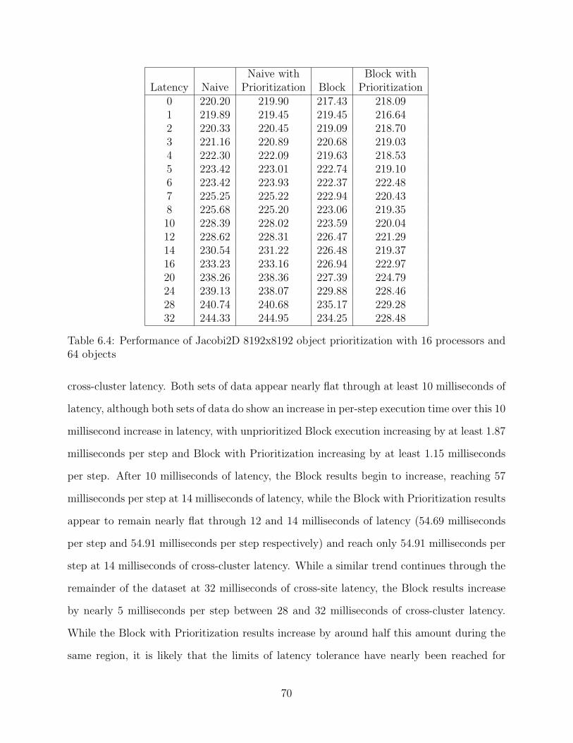
Naive with Block withLatency Naive Prioritization Block Prioritization
0 220.20 219.90 217.43 218.091 219.89 219.45 219.45 216.642 220.33 220.45 219.09 218.703 221.16 220.89 220.68 219.034 222.30 222.09 219.63 218.535 223.42 223.01 222.74 219.106 223.42 223.93 222.37 222.487 225.25 225.22 222.94 220.438 225.68 225.20 223.06 219.3510 228.39 228.02 223.59 220.0412 228.62 228.31 226.47 221.2914 230.54 231.22 226.48 219.3716 233.23 233.16 226.94 222.9720 238.26 238.36 227.39 224.7924 239.13 238.07 229.88 228.4628 240.74 240.68 235.17 229.2832 244.33 244.95 234.25 228.48
Table 6.4: Performance of Jacobi2D 8192x8192 object prioritization with 16 processors and64 objects
cross-cluster latency. Both sets of data appear nearly flat through at least 10 milliseconds of
latency, although both sets of data do show an increase in per-step execution time over this 10
millisecond increase in latency, with unprioritized Block execution increasing by at least 1.87
milliseconds per step and Block with Prioritization increasing by at least 1.15 milliseconds
per step. After 10 milliseconds of latency, the Block results begin to increase, reaching 57
milliseconds per step at 14 milliseconds of latency, while the Block with Prioritization results
appear to remain nearly flat through 12 and 14 milliseconds of latency (54.69 milliseconds
per step and 54.91 milliseconds per step respectively) and reach only 54.91 milliseconds per
step at 14 milliseconds of cross-cluster latency. While a similar trend continues through the
remainder of the dataset at 32 milliseconds of cross-site latency, the Block results increase
by nearly 5 milliseconds per step between 28 and 32 milliseconds of cross-cluster latency.
While the Block with Prioritization results increase by around half this amount during the
same region, it is likely that the limits of latency tolerance have nearly been reached for
70

Naive with Block withLatency Naive Prioritization Block Prioritization
0 54.75 55.03 52.71 52.101 55.09 54.61 52.55 52.732 55.33 54.89 54.67 54.413 57.49 58.02 54.60 53.094 57.94 57.83 54.95 52.795 57.58 57.35 55.12 53.156 58.74 58.35 56.28 54.317 60.27 60.01 56.94 55.798 61.29 60.81 56.97 53.4010 61.17 61.62 54.58 53.2512 62.45 62.20 55.76 54.6914 62.56 62.89 57.00 54.9116 64.45 64.51 58.57 56.0720 65.95 65.81 61.25 58.9824 66.28 66.55 61.09 59.6428 70.25 70.32 64.25 61.5632 74.05 74.34 69.16 64.03
Table 6.5: Performance of Jacobi2D 8192x8192 object prioritization with 64 processors and256 objects
this problem by this point and that extending the dataset beyond 32 milliseconds of latency
would rapidly show both Block and Block with Prioritization results increasing linearly.
6.4 Limitations
The discussion in the previous section highlights some limitations of the object prioritization
technique. Perhaps the most important limitation is that the technique can be applied only
in situations where most of the processors in each cluster of a Grid computation have a
favorable ratio of a small number of border objects mixed with a larger number of local-
only objects. This allows the border objects to be prioritized and driven in a more useful
way by the Charm++ Scheduler such that the best use is made of the work driven in the
local-only objects. Furthermore, the number of objects per processor must be in a sort of
“sweet spot” between too few objects, where little or no work exists for the purposes of
71

latency masking, and too many objects, where increasing cross-site latency tends to cause
the per-step application execution time to abruptly shift from flat to linear. Seen another
way, the prioritization technique delays the onset of the latency-dominated regime in each
graph, tolerating somewhat larger latencies than non-prioritized techniques.
Another limitation of the object prioritization technique is that it is implemented in terms
of chare arrays in the Charm++ kernel. As described in Section 2.1, chare arrays are indexed
collections of Charm++ objects that allow all objects in the array to be addressed simulta-
neously or allow objects in the array to be addressed individually. The implementation relies
on border objects to register themselves with the Charm++ kernel so that incoming mes-
sages, which carry header information describing the destination object in terms of an array
ID along with one or more index values into the array, can be placed into the high-priority
Grid Queue or the low-priority Scheduler Queue. In practice, this limitation is not much
of a problem because most modern Charm++ programs are implemented in terms of chare
arrays, including all Adaptive MPI applications due to the fact that AMPI is implemented
using chare arrays internally.
6.5 Summary
This chapter has introduced a technique for improving the performance of tightly-coupled
parallel applications running in Grid computing environments by prioritizing the execution
of the border objects that communicate with neighbors located on remote clusters. The
technique is an optimization to the latency masking technique described in Chapter 4. By
prioritizing the execution of the border objects on each processor, better use is made of the
locally-driven objects for the purposes of masking the effects of cross-cluster latency in a
Grid environment.
The technique in this chapter is best suited for situations in which the number of objects
on each processor is enough to partially, but not entirely, mask the effects of cross-site la-
72

tency. These situations tend to be limited to the regions of performance graphs in which an
application is in the process of shifting from a completely latency-tolerant regime to a com-
pletely latency-dominated regime. In practice, these regions may be limited in size. Further,
in the case of practical non-benchmark applications running in actual Grid environments,
both the granularity of the problem and the latency separating parts of the computation
are likely fixed at values that cannot easily be changed. Unless these values happen to fall
within a fortunate range for a given problem, object prioritization is unlikely to significantly
improve application performance. Finally, even in the best circumstances, the performance
benefits of using object prioritization seem to be on the order of only a few percent improve-
ment. Further work should investigate whether the technique can be improved to give better
results over a more broad range of latencies.
73

Chapter 7
Grid Topology-Aware Load Balancing
Chapter 4 describes the primary architectural technique of this thesis for efficiently executing
tightly-coupled parallel applications in Grid computing environments. This technique uses
message-driven objects within the runtime system layer to mask the effects of cross-cluster
latency. Chapter 5 demonstrates that the latency tolerance capabilities of the Charm++
runtime system can be optimized by carefully mapping objects to processors such that each
processor holds a relatively small number of border objects and a much larger number
of local-only objects. Such a mapping provides every processor with approximately the
same amount of locally-driven work to use in masking wide-area latency, ensuring that each
processor can make forward progress in the computation at about the same rate.
This chapter presents a set of optimization techniques in which the objects in a tightly-
coupled application are dynamically load balanced during execution to improve performance
in Grid environments. These techniques leverage the Charm++ load balancing frame-
work [55] coupled with knowledge of the computational resources and communication topol-
ogy of a Grid environment. The optimizations are applicable to situations where a com-
putation contains a reasonably large number of objects that can be mapped to processors
within the computation to effect an improvement in performance. The aim of the techniques
explored in this chapter is to achieve performance comparable to ad-hoc application-specific
object mapping using much more general purpose automatic techniques.
Load balancing is traditionally a challenging and important topic in parallel computing
due to the fact that many tightly-coupled parallel applications are dynamic in nature. That
is, the computational requirements of an application can change as the application executes
74

due to factors such as progress in a simulation or refinement in an iterative solver. In a
Grid environment, however, load balancing is more challenging and more important because
computational resources can be heterogeneous and because the environment itself can change
as an application executes. For example, the processors in one cluster may be faster than
the processors in another cluster, or the latency between clusters may increase or decrease
as an application executes due to external network traffic. Thus, it may be difficult or
impossible for a human to optimize a Grid application based only on a priori knowledge of
the environment.
The specific techniques employed by Grid topology-aware load balancers can vary greatly
in complexity. The primary objective common to the load balancers developed in this thesis
is to ensure that the processors in a computation are balanced in terms of CPU utilization.
In a Grid environment, successfully addressing this objective requires recognizing that the
processors used within a single job may be of heterogeneous performance and allocating
work accordingly. Beyond this primary objective, the three load balancers presented here
attempt to achieve secondary objectives aimed at optimizing the object-to-object commu-
nication characteristics of a Grid computation. Section 7.1 describes a basic load balancing
technique in which the border objects and local-only objects in each cluster of a Grid com-
putation are distributed evenly among the processors in each cluster. Section 7.2 describes
a much more complex load balancing technique in which the communication graph of a
Grid application is optimized using graph partitioning algorithms to reduce the volume of
cross-cluster communication as well as the volume of communication within each cluster.
Finally, Section 7.3 describes a hybrid load balancing technique that attempts to leverage
the best characteristics of the first two balancers, using graph partitioning to optimize cross-
cluster communication and the even distribution of border objects and local-only objects to
optimize communication internal to each cluster.
75
7.1 Basic Grid Communication Load Balancing
This section describes a very simple Grid-aware load balancer, called GridCommLB, that
attempts to balance a computation based on the measured CPU load and communication
characteristics of individual objects. Because no relationship between objects is considered,
the design and implementation of the technique used in this load balancer is straightforward.
Thus, GridCommLB represents a good starting point for Grid-aware load balancing.
7.1.1 Load Balancer Technique
Recall from the discussion in Chapter 4 that the basic latency tolerance capabilities of
Charm++ and Adaptive MPI are due to the runtime system’s ability to overlap the time
spent waiting for messages to travel between clusters with work driven on each processor in
local-only objects. The technique employed by GridCommLB is a simple corollary to this
observation that attempts to optimize the performance of a Grid computation by distributing
the border objects and local-only objects in each cluster evenly among the processors in the
cluster while at the same time ensuring that each processor is allocated an amount of work
proportional to its relative performance. A major advantage of the technique is that it can
be implemented and executed very simply. By observing which objects send messages to
neighbors on remote clusters, the border objects can be identified. When load balancing
takes place, these objects can then be balanced independently without considering their
relationship with other objects in the computation at any more extensive level.
No objects are ever migrated across cluster boundaries in the simple technique devel-
oped in GridCommLB. That is, every object remains somewhere in the cluster in which it is
originally mapped. This greatly simplifies the implementation of the load balancer because
each cluster is load balanced independently of the other clusters in the computation. This
assumes, however, that the objects are initially mapped to processors mostly uniformly. For
most Charm++ applications, this is likely a safe assumption. For the case of Adaptive MPI
76
applications, AMPI handles the task of assigning virtual processors to physical processors,
and this assignment is such a uniform mapping. If objects are not mapped somewhat uni-
formly, overall application performance can suffer with GridCommLB due to the processors
in one cluster being overloaded in terms of work relative to the amount of work being done
in other clusters.
7.1.2 Implementation Details
Based on the description of the general technique described in the previous section, the im-
plementation of GridCommLB is reasonably straightforward. During application execution,
the Charm++ load balancing framework collects statistics about the runtime characteristics
of the objects in the application. Such statistics include the measured CPU load of each
object as well as information about the number of messages and number of bytes sent be-
tween every pair of objects. For each communication event that takes place within a load
balancing period, the source object and destination object for the event are examined. The
corresponding processors upon which the source and destination objects reside are also de-
termined by examining a vector supplied by the load balancing framework that contains the
current object-to-processor mapping. Finally, the clusters in which the source and destina-
tion processors reside are determined based on information provided by the user or probed
automatically by the runtime system during program startup. If the source and destination
processors reside in different clusters, the count of wide-area messages and message bytes for
the source object is incremented; otherwise the count for local-area messages and message
bytes is incremented.
After all communication events are examined, objects can be migrated to new destination
processors based on the amount of wide-area communication they have done during the past
load balancing period. Because the basic load balancing technique does not migrate objects
across cluster boundaries, each cluster is considered independently when making migration
decisions. For each cluster, objects are iteratively placed onto processors by means of a
77

greedy algorithm in which the current heaviest object is mapped onto the lightest loaded
processor. To map an object onto a processor, the object’s entry in a vector is updated
to reflect the new mapping. The process repeats until all of the objects located on the
current cluster have been mapped to processors. The overall process is then repeated for
the remaining clusters in the computation. At the end of load balancing, the Charm++
load balancing framework uses the new object-to-processor mapping vector to update the
positions of all objects in the computation.
The greedy algorithm used to identify the current heaviest object is slightly more complex
than simply choosing the object with the largest number of cross-cluster communication
events. Using the number of cross-cluster communication events as the only criteria for
selecting the next object to migrate can lead to large CPU load imbalances throughout
the computation as some processors become overloaded with work despite the fact that all
processors are balanced in terms of the number of border objects and local-only objects.
Instead, the greedy algorithm must take into consideration both the measured CPU load of
each object as well as the number of cross-cluster messages of each object when selecting the
heaviest object for load balancing. The process by which this is carried out in GridCommLB
is as follows. First, all objects in the current cluster are examined to determine the object
with the largest measured CPU load as well as the object with the largest number of cross-
cluster messages. If the object with the largest measured CPU load happens to also be
the object with the largest number of cross-cluster messages, or happens to have a cross-
cluster message count matching that of the object with the largest number of cross-cluster
messages, then this object is the overall heaviest object in the cluster and can be mapped
next. Otherwise, all objects in the current cluster are examined again to identify the objects
that have a measured CPU load within a given tolerance of the maximum CPU load. This
tolerance defaults to a value of 10%, although it can be adjusted by the user at runtime. Of
the objects that have a measured CPU load within the specified tolerance of the maximum
measured CPU load, the object with the largest number of cross-cluster messages is selected
78
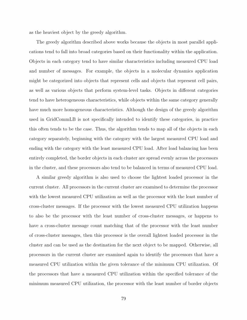
as the heaviest object by the greedy algorithm.
The greedy algorithm described above works because the objects in most parallel appli-
cations tend to fall into broad categories based on their functionality within the application.
Objects in each category tend to have similar characteristics including measured CPU load
and number of messages. For example, the objects in a molecular dynamics application
might be categorized into objects that represent cells and objects that represent cell pairs,
as well as various objects that perform system-level tasks. Objects in different categories
tend to have heterogeneous characteristics, while objects within the same category generally
have much more homogeneous characteristics. Although the design of the greedy algorithm
used in GridCommLB is not specifically intended to identify these categories, in practice
this often tends to be the case. Thus, the algorithm tends to map all of the objects in each
category separately, beginning with the category with the largest measured CPU load and
ending with the category with the least measured CPU load. After load balancing has been
entirely completed, the border objects in each cluster are spread evenly across the processors
in the cluster, and these processors also tend to be balanced in terms of measured CPU load.
A similar greedy algorithm is also used to choose the lightest loaded processor in the
current cluster. All processors in the current cluster are examined to determine the processor
with the lowest measured CPU utilization as well as the processor with the least number of
cross-cluster messages. If the processor with the lowest measured CPU utilization happens
to also be the processor with the least number of cross-cluster messages, or happens to
have a cross-cluster message count matching that of the processor with the least number
of cross-cluster messages, then this processor is the overall lightest loaded processor in the
cluster and can be used as the destination for the next object to be mapped. Otherwise, all
processors in the current cluster are examined again to identify the processors that have a
measured CPU utilization within the given tolerance of the minimum CPU utilization. Of
the processors that have a measured CPU utilization within the specified tolerance of the
minimum measured CPU utilization, the processor with the least number of border objects
79

is considered to be the lightest processor. If two processors that are both within the specified
tolerance have an equal number of border objects, the processor with the least number of
cross-cluster messages is considered to be the lightest processor.
Because the processors within a cluster may be of heterogeneous performance, the greedy
algorithm for choosing the lightest loaded processor must also scale the measured CPU loads
of the objects placed onto a processor based on the processor’s measured performance. For
example, some clusters in the core TeraGrid [1] have processors of heterogeneous performance
with some 1.3 GHz processors and some 1.5 GHz processors. When the Charm++ load bal-
ancing framework is initialized, the speed of each processor is measured and made available
to the load balancers to use in whatever way they choose. GridCommLB uses this informa-
tion to map more objects onto faster processors in each cluster. Thus in the example of the
TeraGrid clusters, any 1.3 GHz processors used in a computation would receive only about
85% of the work mapped onto any 1.5 GHz processors in the computation. However, because
the technique used by GridCommLB never migrates objects across cluster boundaries, more
work cannot be allocated to remote clusters that are composed entirely of better-performing
processors. Unfortunately, this seems to be a more likely scenario for heterogeneity in a Grid
computation, with one cluster being composed entirely of the same performance of processor
and another cluster being composed entirely of the same higher-performance processor.
Finally, an assumption made during the implementation of GridCommLB is that all
communication operations taking place in the computation are of the same weight. No
differentiation is made between very small messages and very large messages when making
load balancing decisions. Only the absolute number of communication events that an object
is involved in is considered as a basis for load balancing.
80

7.1.3 Performance Evaluation
The performance of GridCommLB was evaluated using the five-point stencil benchmark
introduced in Chapter 4. Problem sizes of 2048x2048 and 8192x8192 were evaluated. In
all experiments, Naive mapping was used to initially map objects onto processors and then
GridCommLB was invoked to load balance the application by adjusting the object mapping
based on measured CPU load and number of cross-cluster messages sent by each object.
Figures 7.1, 7.2, 7.3, and 7.4 show the results for the 2048x2048 problem size for 8, 16, 32,
and 64 processors respectively. For the graphs corresponding to the lowest number of objects
per processor (Figures 7.1(a), 7.2(a), 7.3(a), and 7.4(a)), little or no change is apparent in
the results for GridCommLB. This is expected due to the fact that each processor holds only
one or two objects in these configurations, so the load balancer has little or no opportunity
to make useful adjustments in these cases. Unfortunately, however, as the number of objects
per processor increases, the load balancer still produces little or no change in performance
from the starting point Naive mapping performance. This is also the case in the larger
8192x8192 problem size results shown in Figures 7.5, 7.6, 7.7, and 7.8.
In many ways, the Jacobi2D benchmark is a worst-case scenario for the load balancing
technique employed by GridCommLB due to the fact that the objects have nearly identical
measured CPU loads and communication characteristics. The GridCommLB load balancer
works by balancing the objects in a computation on their measured CPU loads while ad-
ditionally spreading the border objects and local-only objects evenly among the processors
in each cluster. In a simple benchmark like Jacobi2D, overloading any processor by even
a single object produces a very noticeable degradation in performance. So, in some ways,
the fact that performance does not get worse after load balancing is a useful result for these
experiments. Further, the expectation is that any improvements to latency masking due
to the load balancing strategy employed by GridCommLB will only really be noticeable as
latency increases. That is, the useful effects of GridCommLB would primarily be seen on
81

(a) Processors = 8, Number of Objects = 16 (b) Processors = 8, Number of Objects = 64
(c) Processors = 8, Number of Objects = 256 (d) Processors = 8, Number of Objects = 1024
Figure 7.1: Performance of Jacobi2D 2048x2048 with GridCommLB (8 processors)
82
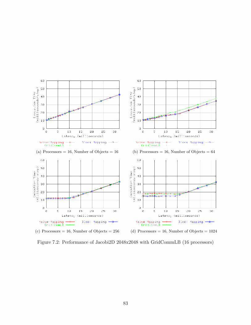
(a) Processors = 16, Number of Objects = 16 (b) Processors = 16, Number of Objects = 64
(c) Processors = 16, Number of Objects = 256 (d) Processors = 16, Number of Objects = 1024
Figure 7.2: Performance of Jacobi2D 2048x2048 with GridCommLB (16 processors)
83

(a) Processors = 32, Number of Objects = 64 (b) Processors = 32, Number of Objects = 256
(c) Processors = 32, Number of Objects = 1024 (d) Processors = 32, Number of Objects = 4096
Figure 7.3: Performance of Jacobi2D 2048x2048 with GridCommLB (32 processors)
84
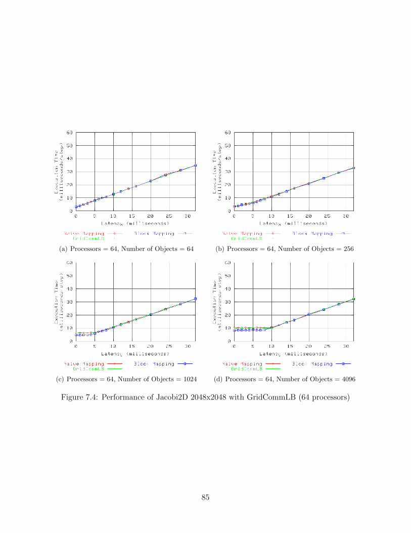
(a) Processors = 64, Number of Objects = 64 (b) Processors = 64, Number of Objects = 256
(c) Processors = 64, Number of Objects = 1024 (d) Processors = 64, Number of Objects = 4096
Figure 7.4: Performance of Jacobi2D 2048x2048 with GridCommLB (64 processors)
85

(a) Processors = 8, Number of Objects = 16 (b) Processors = 8, Number of Objects = 64
(c) Processors = 8, Number of Objects = 256 (d) Processors = 8, Number of Objects = 1024
Figure 7.5: Performance of Jacobi2D 8192x8192 with GridCommLB (8 processors)
the righthand sides of the performance graphs. For the larger 8192x8192 problem size, most
of the performance graphs are near horizontal, indicating complete latency tolerance due
to the Charm++ runtime system finding enough work to fill in otherwise-wasted idle time
on each processor. For the smaller 2048x2048 problem size, the righthand portions of each
graph where latency is not entirely masked do not show significantly different performance
between the Naive mapping of objects and the Block mapping of objects. In more complex
problems, such as those examined as case studies in Chapter 8, GridCommLB does make
noticeable improvements in application performance.
86
(a) Processors = 16, Number of Objects = 16 (b) Processors = 16, Number of Objects = 64
(c) Processors = 16, Number of Objects = 256 (d) Processors = 16, Number of Objects = 1024
Figure 7.6: Performance of Jacobi2D 8192x8192 with GridCommLB (16 processors)
87

(a) Processors = 32, Number of Objects = 64 (b) Processors = 32, Number of Objects = 256
(c) Processors = 32, Number of Objects = 1024 (d) Processors = 32, Number of Objects = 4096
Figure 7.7: Performance of Jacobi2D 8192x8192 with GridCommLB (32 processors)
88

(a) Processors = 64, Number of Objects = 64 (b) Processors = 64, Number of Objects = 256
(c) Processors = 64, Number of Objects = 1024 (d) Processors = 64, Number of Objects = 4096
Figure 7.8: Performance of Jacobi2D 8192x8192 with GridCommLB (64 processors)
89

7.1.4 Overhead
The algorithm that GridCommLB uses to identify the heaviest object and lightest processor
is a linear search. Because a typical Charm++ program has many more objects than proces-
sors, GridCommLB is bounded by an asymptotic running time of O(n2) for a computation
with n objects. A trivial optimization is possible by using heap data structures to hold
the list of objects and the list of processors. This optimization would allow the asymptotic
running time to be reduced to O(n ∗ log(n)).
Table 7.1 shows the amount of time required to balance the Jacobi2D examples shown in
the previous section. “Strategy Time” is the time required by GridCommLB itself. “Load
Balancing Time” is the entire amount of time required to complete the load balancing
operation, including the time to set up the data structures that are passed to the load
balancer, the time to execute the load balancer strategy, and the time to migrate all objects
to new processors. Even in the case of 4096 objects, the maximum for any application in
this thesis including the case study applications described in Chapter 8, the time required
by GridCommLB is approximately 250 milliseconds while the overall load balancing time is
less than one second.
7.1.5 Limitations
The basic communication load balancing technique used by GridCommLB presents a good
starting point for Grid-aware load balancing due to its simplicity. In more complex appli-
cations than the simple Jacobi2D benchmark used in this chapter, such as the molecular
dynamics application studied in Chapter 8, GridCommLB can achieve good improvements
in performance by balancing on the measured CPU load of each object in addition to evenly
distributing the border objects and local-only objects across the processors in a cluster. In
practice, the improvements seen by GridCommLB are on par with those achieved by mea-
sured CPU load balancing alone, and can exceed measured CPU load balancing in situations
90

Number of Number of Strategy Time Load Balancing TimeProcessors Objects (seconds) (seconds)
8 16 0.000063 0.1645438 64 0.000190 0.1526178 256 0.001307 0.1629198 1024 0.017534 0.24530016 16 0.000065 0.12248216 64 0.000217 0.11356416 256 0.001371 0.17317116 1024 0.016811 0.18985532 64 0.000242 0.10207232 256 0.001542 0.13984932 1024 0.017486 0.17190732 4096 0.265889 0.50459064 64 0.000317 0.08606564 256 0.001621 0.09822164 1024 0.021951 0.15921164 4096 0.263361 0.637086
Table 7.1: Overhead of the basic load balancing technique in GridCommLB
of high cross-cluster latency.
One limitation of the basic communication load balancing technique is that objects are
never migrated across cluster boundaries. In theory, situations where an application was
running in a Grid environment with a large number of very small clusters would likely result
in CPU load imbalances throughout the computation due to some objects with extremely
high CPU loads being “trapped” on a fixed cluster. In practice, however, the number of
clusters used in a realistic Grid application is likely to be small, on the order of two to four,
so this limitation is possibly not critical.
The biggest limitation of the basic communication load balancing technique is that it
has no way of identifying the communication relationship between objects. This is evident
in the results shown in Section 7.1.3. Because all objects in the Jacobi2D benchmark have
approximately the same measured CPU load, the balancer can make little or no improve-
ment by remapping objects to optimize processor utilization. For this problem, the largest
possible improvements are related to the structure of the communications in the application,
91

as demonstrated by the differences in performance between the Naive and Block mapping
strategies discussed in Chapter 5. Since GridCommLB does not identify the communication
relationship between objects, however, it cannot arrange objects into block-type structures
that improve the communications volume internal to each cluster. Thus, the only benefits
achievable by GridCommLB are those that results from improved latency tolerance due to
distributing the border objects and local-only objects in an application evenly among the
processors in each cluster. As shown in Section 7.1.3, this optimization results in only a
subtle improvement in performance for the Jacobi2D benchmark in most cases.
7.2 Graph Partitioning Load Balancing
The previous section describes a basic communication load balancing technique that dis-
tributes the border objects and local-only objects in an application evenly among the pro-
cessors in each cluster while simultaneously ensuring that each processor is allocated an
amount of work proportional to its relative performance. This technique is quite limited
because it does not identify any relationship between the objects in a computation. In a
tightly-coupled Grid application, however, identifying the relationship between objects and
optimizing the application accordingly is crucial for achieving good performance.
This section describes a load balancing technique based on partitioning the communica-
tion graph of the application to reduce the volume of cross-cluster communication and the
volume of communication within each cluster. Graph partitioning improves significantly on
the technique of the previous section by identifying the relationship between objects and
load balancing the computation to reflect this relationship.
7.2.1 Load Balancing Technique
A Grid computation can be thought of as representing a hierarchy of communication laten-
cies. At the lowest level of this hierarchy is lightweight intra-processor communication, such
92
as when two neighboring objects are co-located on the same processor. The next level of
the hierarchy is represented by slightly heavier weight intra-cluster communication, such as
when two neighboring objects are co-located within the same cluster. Finally, at the highest
level of the hierarchy, heavy-weight cross-cluster communication is used when two neighbor-
ing objects must communicate with each other over high-latency wide-area communication
channels. Latencies within this hierarchy can vary from sub-microsecond intra-processor
latencies, to intra-cluster latencies measured in tens of microseconds, and finally to cross-
cluster latencies measured in tens or hundreds of milliseconds.
If the relationship between objects in a tightly-coupled parallel application can be de-
termined and used in conjunction with knowledge of the communication hierarchy of the
Grid environment itself, much better improvements in performance are possible than with
the basic Grid communication load balancing technique described in the previous section.
One possible way of doing this is by using graph partitioning techniques to find a favorable
“cut” in the communication graph of the objects in an application and thereby reduce the
volume of cross-cluster communication required in the application. By reducing the vol-
ume of cross-cluster communication in the application overall and then using the latency
masking architecture of the Charm++ runtime system described in Chapter 4, very good
performance is possible with tightly-coupled applications in Grid computing environments.
7.2.2 Implementation Details
The first step in creating a Grid topology-aware graph partitioning load balancer is discov-
ering where the discrete breaks in the communication hierarchy are located. In the case of
intra-processor latencies, this is trivial – the actual processors allocated to the computation
define these boundaries. In the case of cross-cluster latencies, all that is necessary is to deter-
mine which processors belong to each cluster. This information is available to the Charm++
load balancing framework based on information provided by the user or probed automat-
ically by the runtime system during program startup. This overall information about the
93

communication hierarchy of a Grid job is then used to make topology-aware load balancing
decisions.
After the topology of a Grid computation is discovered, the next step is to load bal-
ance the running application to reflect this topology based on the statistics collected by the
Charm++ load balancing framework about each object’s measured CPU load and commu-
nication with other objects. To do this, a favorable mapping of objects to processors can be
computed by using graph partitioning techniques to produce a better cut in the object com-
munication graph across cluster boundaries. Ideally, this would be a minimal cut resulting
in the smallest volume of cross-cluster traffic that is theoretically possible. Unfortunately,
graph partitioning is NP-complete and determining a minimal cut in the communication
graph is computationally infeasible for non-trivial numbers of objects. Efficient heuristic
procedures for partitioning arbitrary graphs exist that are both effective in finding optimal
partitions and fast enough to be practical for use in applications with non-trivial numbers
of objects [31]. Several software packages exist that further refine these heuristic techniques
by applying fast approximations to reduce the time required to find a good solution. These
software packages include Metis [28, 26, 25, 27], Chaco [19], Jostle [52, 51, 53, 50], and
Scotch [43]. The implementation of a Grid topology-aware graph partitioning load balancer
described here uses Metis, although this choice was arbitrary based on familiarity with the
software and it is expected that any of the other efficient graph partitioners could be used
with similar results. The resulting load balancer implementing the technique of this chapter
is called GridMetisLB.
Simply partitioning the object communication graph into a number of partitions equal
to the number of processors in the computation would not result in an optimal mapping,
because this mapping would not reflect the fact that the inter-processor latency between
some pairs of processors is much greater than the latency between other pairs in a Grid
computation. Instead, a two-phase algorithm is used to partition objects onto processors
while producing a better volume of communication in the communication graph across cluster
94

boundaries. This algorithm is described as follows.
• Phase 1: In the first phase, objects are partitioned into the clusters in the Grid
computation. At this stage, no consideration is given to balancing the computation on
the measured CPU load of each object. Rather, the sole criteria for balancing is the
measured number of object-to-object messages. This is to ensure that the partitioning
of objects produced in this phase results in as good of a cut as possible with the
heuristics used by Metis on the edges of the communication graph that cross cluster
boundaries.
To carry out this phase, a graph is constructed for input to Metis that includes every
object in the computation. Weights on the edges of the graph represent the number
of messages passed between any pair of objects. Vertex weights are ignored. Metis
is then instructed to partition the communication graph into a number of partitions
related to the number of clusters in the computation. In some cases, the number of
partitions used may not necessarily be exactly equal to the number of clusters in the
computation, and this discrepancy is described below.
• Phase 2: In the second phase, objects within each cluster are partitioned onto the
processors within their assigned clusters. This partitioning considers both the mea-
sured CPU load of each object as well as the object-to-object communication graph
internal to each cluster, producing an object mapping that likely improves the volume
of internal cluster communication while simultaneously attempting to balance the CPU
utilization of each processor. Inter-object communication that crosses cluster bound-
aries is ignored at this phase due to the fact that Phase 1 above determines a favorable
edge cut across cluster boundaries as long as each border object appears anywhere
within the cluster to which it was assigned in Phase 1.
To carry out this phase, graphs are constructed for input to Metis that includes every
object in each cluster. Weights on the edges of these graphs represent the number of
95
messages passed between objects. Vertex weights represent the measured CPU load of
each object. Metis is then instructed to partition the graph into a number of partitions
related to the number of processors in the associated cluster. Again, in some cases,
the number of partitions used may not necessarily be exactly equal to the number of
processors in a given cluster, and this discrepancy is described below.
After completing this two-phase process, the resulting object mapping is likely such that
all objects in the computation have been balanced to produce a favorable cut in the object
communication graph that reduces the volume of communication across cluster boundaries,
as well as in a way that balances CPU utilization and intra-cluster object communication
within each cluster.
As mentioned previously, the number of partitions requested from Metis in the phases of
the algorithm described above may not necessarily exactly match the number of clusters in
the computation (Phase 1) or the number of processors in a given cluster (Phase 2). This
discrepancy is due to the possibility of a heterogeneous allocation of resources used in a
Grid computation. For example, the processors within a single cluster may be of varying
speeds. In such a case, it is desirable to allocate more work to the faster processors and
less work to the slower processors. In order to get Metis to do this, the measured CPU
speed of each processor, collected automatically by the Charm++ load balancing framework
during program startup and initialization, is normalized against the slowest processor in each
cluster. This produces a multiplier for each processor; the sum of these multipliers is used
as the number of partitions for Metis. The resulting object map from Metis is then related
to the physical processors in terms of this multiplier. That is, a processor that is twice as
fast as the slowest processor in its cluster receives a multiplier of two, and is accordingly
assigned objects from two partitions of the object map produced by Metis. Similarly, and
more likely in a real Grid computation, clusters may be of unequal power, due either to an
unequal number of processors (e.g., Cluster A has twice as many processors as Cluster B)
or to heterogeneous processor speeds between clusters. The solution here is to compute a
96

multiplier for each cluster, based on the sum of the multipliers for the processors that make
up each cluster, and to use the sum of these as the number of partitions for Metis.
7.2.3 Performance Evaluation
The performance of GridMetisLB was evaluated using the Jacobi2D benchmark introduced
in Chapter 4. Problem sizes of 2048x2048 and 8192x8192 were evaluated. In all experiments,
Naive mapping was used to initially map objects onto processors and then GridMetisLB was
invoked to load balance the application by adjusting the object mapping based on measured
CPU load and number of messages sent between each pair of objects.
Figures 7.9, 7.10, 7.11, and 7.12 show the results for the 2048x2048 problem size for 8,
16, 32, and 64 processors respectively. For the graphs corresponding to the lowest number
of objects per processor (Figures 7.9(a), 7.10(a), 7.11(a), and 7.12(a)), little or no change
is apparent in the results for GridMetisLB. This is expected due to the fact that each
processor holds only one or two objects in these configurations, so the load balancer has
little or no opportunity to make useful adjustments in these cases. As the number of objects
per processor begins to increase, the load balancer begins to show some improvements to
the performance of the computation. For example, for the configuration with 8 processors
and 64 objects (Figure 7.9(b)), the load balanced results improve on the Naive mapping
results between 10 and 24 milliseconds of cross-cluster latency. The results are not entirely
consistent, however, as in the case of 16 processors and 64 objects (Figure 7.9(b)) where
the load balanced results are actually worse from 12 through 32 milliseconds of cross-cluster
latency. This discrepancy from the results in the previous graph make some sense, though,
as this problem size gives the load balancer only 4 objects per processor with which to work
while the previous problem gives the load balancer 8 objects per processor. The similar
configurations for 32 processors and 256 objects (Figure 7.11(b)) and 64 processors and 256
objects (Figure 7.12(b)) show little or no improvements due to load balancing. These results
make sense here, however, because for these problem sizes there is little or no difference
97

between the performance of Naive mapping and Block mapping for object placement. The
intuition, then, is that rearranging the mapping of objects to processors cannot improve the
performance for these configurations in any appreciable way.
The configurations where GridMetisLB performs exceptionally well are those involving
a more generous number of objects per processor in the computation (Figures 7.9(c) and
7.9(d), 7.10(c) and 7.10(d), 7.11(c) and 7.11(d), and 7.12(c) and 7.12(d)). In these graphs,
GridMetisLB is able to identify object mappings that give performance matching that of
Block mapping. In many ways, the Jacobi2D benchmark is an ideal scenario for the load
balancing technique employed by GridMetisLB due to the fact that the objects have nearly
identical measured CPU loads and communication characteristics. It is no coincidence that
the results for load balancing closely match those of Block mapping. When GridMetisLB
takes the Grid topology into consideration by partitioning the object communication graph
in such a way as to reduce the volume of communication across the cross-cluster boundary
(Phase 1) as well as the volume of communication between processors within each cluster
(Phase 2), it is in fact mapping objects to processors in a block-oriented structure. Further,
this explains why the results for load balancing in Figure 7.12(d) for 64 processors and 4096
objects are better than the results for Block mapping. Recall from the discussion in Sec-
tion 5.2 that the mapping strategy that results in the minimum amount of inter-processor
communication is a square mapping, and that the use of Block mapping in this thesis is
simply a convenient approximation. For the case of 64 processors and 4096 objects, Grid-
MetisLB arranges the objects into a mapping that results in an even lower communication
volume than Block mapping.
Figures 7.13, 7.14, 7.15, and 7.16 show the results for the 8192x8192 problem size for
8, 16, 32, and 64 processors respectively. The results here are similar to the results for
the smaller problem size. As before, the most noticeable improvements in performance due
to load balancing are in the configurations with larger numbers of objects per processor.
The results for 8 processors and 1024 objects (Figure 7.13(d)), 16 processors and 1024
98

(a) Processors = 8, Number of Objects = 16 (b) Processors = 8, Number of Objects = 64
(c) Processors = 8, Number of Objects = 256 (d) Processors = 8, Number of Objects = 1024
Figure 7.9: Performance of Jacobi2D 2048x2048 with GridMetisLB (8 processors)
99

(a) Processors = 16, Number of Objects = 16 (b) Processors = 16, Number of Objects = 64
(c) Processors = 16, Number of Objects = 256 (d) Processors = 16, Number of Objects = 1024
Figure 7.10: Performance of Jacobi2D 2048x2048 with GridMetisLB (16 processors)
100

(a) Processors = 32, Number of Objects = 64 (b) Processors = 32, Number of Objects = 256
(c) Processors = 32, Number of Objects = 1024 (d) Processors = 32, Number of Objects = 4096
Figure 7.11: Performance of Jacobi2D 2048x2048 with GridMetisLB (32 processors)
101
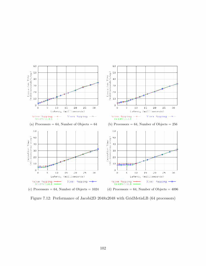
(a) Processors = 64, Number of Objects = 64 (b) Processors = 64, Number of Objects = 256
(c) Processors = 64, Number of Objects = 1024 (d) Processors = 64, Number of Objects = 4096
Figure 7.12: Performance of Jacobi2D 2048x2048 with GridMetisLB (64 processors)
102

(a) Processors = 8, Number of Objects = 16 (b) Processors = 8, Number of Objects = 64
(c) Processors = 8, Number of Objects = 256 (d) Processors = 8, Number of Objects = 1024
Figure 7.13: Performance of Jacobi2D 8192x8192 with GridMetisLB (8 processors)
objects (Figure 7.14(d)), 32 processors and 1024 objects (Figure 7.15(c)), and 32 processors
and 4096 objects (Figure 7.15(d)) in particular demonstrate the ability of GridMetisLB
to improve the performance of the Naive mapping such that the load balanced per-step
execution time closely matches that of Block mapping. Even in the largest problem sizes
where the differences between Naive mapping and Block mapping are not as large (Figures
7.16(c) and 7.16(d)), GridMetisLB still produces results that are noticeably better than the
original Naive mapping starting point.
103

(a) Processors = 16, Number of Objects = 16 (b) Processors = 16, Number of Objects = 64
(c) Processors = 16, Number of Objects = 256 (d) Processors = 16, Number of Objects = 1024
Figure 7.14: Performance of Jacobi2D 8192x8192 with GridMetisLB (16 processors)
104

(a) Processors = 32, Number of Objects = 64 (b) Processors = 32, Number of Objects = 256
(c) Processors = 32, Number of Objects = 1024 (d) Processors = 32, Number of Objects = 4096
Figure 7.15: Performance of Jacobi2D 8192x8192 with GridMetisLB (32 processors)
105

(a) Processors = 64, Number of Objects = 64 (b) Processors = 64, Number of Objects = 256
(c) Processors = 64, Number of Objects = 1024 (d) Processors = 64, Number of Objects = 4096
Figure 7.16: Performance of Jacobi2D 8192x8192 with GridMetisLB (64 processors)
106

7.2.4 Overhead
Graph partitioning, even with good heuristics coupled with optimizations to improve the
performance of the algorithms, is computationally expensive. An efficient heuristic procedure
described by Kernighan and Lin varies with the number of partitions and has a running time
of between O(n2) and O(n2∗log(n)) depending on optimizations that determine the exactness
of the solution found [31]. The implementation of graph partitioning used in Metis varies
by the number of edges in the graph and the number of partitions. Metis uses O(|E|) steps
that are each between O(log(n)) and O(n2) based on the solution found by a randomized
algorithm at each step.
Table 7.2 shows the amount of time required to balance the Jacobi2D examples shown
in the previous section. As before, “Strategy Time” is the time required by GridMetisLB
itself while “Load Balancing Time” is the entire amount of time required to complete the
load balancing operation, including the time to set up the data structures that are passed to
the load balancer, the time to execute the load balancer strategy, and the time to migrate
all objects to new processors. These results clearly show that the superior results obtained
by GridMetisLB come at a somewhat larger cost in terms of computational effort required
by the load balancer when compared to the results for the much simpler GridCommLB in
Table 7.1.
7.2.5 Limitations
The graph partitioning load balancing technique used by GridMetisLB can produce very
good results in tightly-coupled parallel applications running in Grid computing environments
because it takes into consideration the relationship between objects in the computation and
couples this with knowledge of the topology of the Grid resources used to run the applica-
tion. One limitation of this technique is that graph partitioning is quite computationally
expensive. This potentially impacts the use of the technique in realistic applications in two
107

Number of Number of Strategy Time Load Balancing TimeProcessors Objects (seconds) (seconds)
8 16 0.000541 0.2123118 64 0.001075 0.2059828 256 0.004150 0.1914138 1024 0.035866 0.29172816 16 0.000477 0.11879116 64 0.001102 0.12845216 256 0.004395 0.18165616 1024 0.036623 0.26265232 64 0.001302 0.11337532 256 0.004959 0.11785432 1024 0.038734 0.19517432 4096 0.746509 0.98651864 64 0.001629 0.06866064 256 0.005585 0.10235564 1024 0.040867 0.19799864 4096 0.754307 0.995384
Table 7.2: Overhead of the graph partitioning load balancing technique in GridMetisLB
ways. First, the memory requirements necessary for doing graph partitioning may become
prohibitive for very large applications. The data structures required in the implementation
of GridMetisLB to construct representations of the communications graph for input to Metis
consume an amount of memory that varies with the number of objects in the computation.
The asymptotic space complexity of the memory usage is O(n2), although improvements to
data structures could reduce this by half or more. For large computations, tens or hundreds
of megabytes of memory might be required to hold the data structures needed for graph
partitioning. Second, and possibly more critical, the wallclock time required to partition the
communication graph may become large enough that load balancing the application is no
longer worthwhile for very large numbers of objects. That is, the Metis developers report
that graphs with hundreds of thousands of vertices and millions of edges can be partitioned
into several hundred partitions in under a minute. In order for this investment in time to
be worthwhile, the improvements in performance must be large enough to exceed the time
invested in load balancing. Many practical scientific applications run for days or weeks,
108

however, so it seems likely that the benefits of load balancing many realistic applications
would easily offset even a few expensive load balancing operations lasting for several minutes
of the application’s entire execution time.
One possible solution to the two problems outlined above might be to use a parallel
implementation of Metis called ParMetis [29]. Because the application is already running
in a parallel environment, it makes sense also to leverage this resource for the purposes of
load balancing. Doing so could benefit the implementation of GridMetisLB both in terms of
the memory requirements and the wallclock time required to partition the communication
graphs of very large applications. The trade-off of using ParMetis is that it comes at the
cost of additional software complexity.
There are two other significant limitations of the graph partitioning load balancing tech-
nique used by GridMetisLB. First, the graph partitioning algorithm employed by Metis
primarily considers the edge weights of a communication graph and only secondarily con-
siders the vertex weights. Metis attempts to produce partitions of approximately equal size,
although some partitions may end up with a few more objects than others. This means that
the object mapping generated by GridMetisLB may overload some processors in terms of
CPU utilization due to placing more objects on some processors in the computation than oth-
ers. Such a mapping is likely to degrade overall application performance after load balancing
rather than improve it. Second, the object-to-processor mapping generated by GridMetisLB
does not guarantee that the border objects and the local-only objects assigned to a clus-
ter will be evenly spread among the processors in the cluster. The primary observation of
Chapter 5 is that this type of object mapping enhances the latency masking capabilities of
the Charm++ runtime system. Thus, while the object mapping produced by GridMetisLB
is good for optimizing the volume of communication internal to each cluster, it is likely to
be less conducive to optimal application performance as cross-site latency increases.
109

7.3 Hybrid Load Balancing
The previous two sections describe Grid-aware load balancing techniques that range from
the very simple technique of evenly distributing the border objects and local-only objects
across the processors in each cluster, employed by GridCommLB, to the much more complex
technique of using graph partitioning algorithms to reduce the volume of inter-object com-
munication across cluster boundaries and within each cluster, employed by GridMetisLB.
This section describes a load balancing technique that attempts to leverage the most effec-
tive characteristics of the previous two techniques to create a hybrid load balancer called
GridHybridLB.
7.3.1 Load Balancer Technique
The most important characteristic of the basic communication load balancing technique is
that it ensures that each processor is allocated an amount of work proportional to its relative
performance while simultaneously establishing an even distribution of the border objects and
the local-only objects across the processors in each cluster in a Grid computation. Arranging
the objects in this way allows the runtime system to overlap the otherwise-wasted idle time
spent in wide-area communication with locally-driven work as much as possible on each
processor.
The biggest shortcoming of the basic communication load balancing technique is that
it does not migrate objects across cluster boundaries. Because objects remain within the
cluster in which they are initially allocated, no reduction in the overall volume of cross-
cluster communication is possible since messages must still be transferred between clusters
regardless of where the sending object is placed within its (local) cluster and the receiving
object is placed within its (remote) cluster. Additionally, it is possible for the overall CPU
utilizations of the clusters in a Grid computation to be unbalanced relative to each other due
to several high-load objects being “trapped” within a single cluster, unable to be migrated
110

to clusters with lower overall CPU utilization. The more sophisticated graph partitioning
load balancing technique addresses these deficiencies by using graph partitioning algorithms
to examine inter-object communication patterns. The two-phase technique first balances the
communication graph across cluster boundaries, thereby reducing the volume of cross-cluster
communication traffic, and second balances the communication graph within each cluster.
While balancing objects across cluster boundaries is highly desirable, using expensive graph
partitioning algorithms to balance the objects within each cluster may be overkill due to the
fact that latencies within clusters are usually two or three orders of magnitude lower than
latencies between clusters. That is, reducing the volume of communication between clusters
is significantly more important than reducing the volume of communication within clusters.
Furthermore, the graph partitioning technique only attempts to allocate to each processor
an amount of work proportional to its relative performance but does not guarantee that
the final object mapping will have this characteristic, nor does it guarantee that the border
objects and local-only objects will be spread evenly among the processors in each cluster.
With these ideas in mind, the hybrid load balancing technique implemented in GridHy-
bridLB combines the most desirable characteristics of the previous techniques to create a
Grid-aware load balancing solution that can produce potentially superior results. GridHy-
bridLB utilizes a graph partitioning algorithm to do the initial placement of objects onto
clusters, allowing a reduction in the volume of communication traversing cross-cluster bound-
aries as well as allowing objects with high loads to be migrated away from each other. Within
each cluster, GridHybridLB utilizes the approach taken by GridCommLB of allocating a pro-
portional amount of work to each processor, based on relative performance compared to the
other processors in the cluster, while simultaneously establishing an even distribution of
border objects and local-only objects among the processors in the cluster. A refinement to
this approach, described below, identifies communication relationships among the objects
within a cluster and attempts to co-locate neighboring objects in the computation on the
same processor as much as possible. This refinement allows the interprocessor communica-
111

tion volume within each cluster to be reduced at the cost of additional time taken during
load balancing.
7.3.2 Implementation Details
The implementation of GridHybridLB follows directly from the implementations of Grid-
MetisLB and GridCommLB. Like GridMetisLB, the hybrid load balancing technique uses
a two-phase algorithm. The first phase is identical to the first phase of the algorithm em-
ployed by GridMetisLB which partitions objects into the clusters in the Grid computation.
The partitioning of objects produced in this phase cuts the communication graph in the
computation in a way that likely reduces the number of messages that must cross cluster
boundaries. Furthermore, because this phase of the algorithm takes into consideration the
relative overall performance of each cluster, in terms of the number of processors and their
speeds, objects can be allocated to clusters in a way that does not significantly overload any
single cluster.
In the second phase, objects within each cluster are placed onto the processors within
their assigned clusters. This phase can operate in one of three “modes” that may be selected
by the user at runtime. The first mode causes the algorithm to behave identically to the
algorithm employed by GridCommLB within each cluster. That is, the objects are placed
onto processors by means of a greedy algorithm that selects the heaviest object in terms
of the number of cross-cluster communication events and places it on the lightest loaded
processor. The algorithm also employs the technique used by GridCommLB of selecting
better candidate objects that fall within a user-specified tolerance (defaulting to 10%) of
the largest measured CPU load of all unassigned objects in the cluster. Additionally, the
algorithm takes into consideration the relative performance of each processor, assigning
proportionally more work to faster processors. The end result is that each processor in
each cluster is balanced in terms of the number of border objects, the number of local-only
objects, and overall proportional processor utilization. This is a significant improvement
112
over the technique employed by GridMetisLB.
For many computations the simple balancing strategy employed in the second phase is
likely sufficient, given that typical intra-cluster latencies are measured on the order of a few
microseconds. These latencies generally dwarf both the typical inter-cluster latencies in a
Grid computation as well as the typical time consumed performing work in the Charm++
entry methods of many parallel applications. However, an additional mode of operation
may be specified for the second phase of load balancing, allowing objects to be placed onto
processors more intelligently by examining the communication relationship between objects
within each cluster. To do this, the algorithm begins by placing the heaviest objects onto the
lightest processors using the greedy algorithm described previously. Once each processor in
the cluster holds one object, the behavior of the algorithm continues by using the first object
on each processor as a “seed” for selecting additional objects. To do this, the algorithm first
identifies the heaviest remaining object assigned to the cluster as before. Next, the algorithm
examines the border objects that are neighbors in the computation to the already-placed
seed object. Only neighboring border objects that have a measured CPU load within the
user-specified tolerance are considered; this is to ensure that particularly CPU-heavy objects
will still be placed onto processors in a timely manner. Of the neighboring border objects
that fall within the tolerance, the one that communicates the most with the seed object is
chosen as the next object for placement onto the processor. This process continues, using the
subsequent objects placed onto each processor as additional seeds from which the heaviest
neighboring border object is selected. When all border objects assigned to the cluster have
been placed onto processors, the local-only objects are placed onto processors using the
border objects on each processor as seeds. The algorithm concludes when all objects assigned
to the cluster have been placed onto processors. As with the traditional greedy algorithm
employed by GridCommLB, the resulting object mapping causes the processors to be well-
balanced in terms of processor utilization and in terms of the number of border objects and
local-only objects. The seeding algorithm extends these characteristics so that the objects
113

residing on each processor after load balancing also tend to be neighbors in the computation.
7.3.3 Performance Evaluation
As with the previous load balancers, the performance of GridHybridLB was evaluated using
the Jacobi2D benchmark with 2048x2048 and 8192x8192 problem sizes. The second phase
of the hybrid load balancing algorithm was done using the seed technique described in the
implementation details above.
Figures 7.17, 7.18, 7.19, and 7.20 show the results for the 2048x2048 problem size for
8, 16, 32, and 64 processors respectively. The observations and conclusions that can be
made about GridHybridLB directly from these graphs are generally similar to the conclu-
sions drawn about the previous two load balancers. Because the load balancing technique
implemented in GridHybridLB is a hybrid of the previous two load balancing techniques, it
is understandable that the most useful insights are found by comparing the GridHybridLB
performance graphs to the graphs of the previous balancers. Comparing the GridHybridLB
graphs to the congruous GridCommLB graphs (Figures 7.1, 7.2, 7.3, and 7.4) reveals no-
ticeably better results with the hybrid technique, particularly for the problem sizes with the
largest number of objects for a given number of processors. This is apparent by observing
that the GridHybridLB technique improves the performance of the initial Naive mapping
to be much closer to the goal Block mapping performance than the GridCommLB tech-
nique does. Due to the uniform structure of the Jacobi2D benchmark, the first phase of
the GridHybridLB algorithm cannot be responsible for these improvements in performance
since there is no way to reduce the volume of cross-cluster traffic by repartitioning objects
in this problem. Therefore, the performance improvements that GridHybridLB achieves
over GridCommLB must be due to the use of the seed technique in the second phase of
GridHybridLB.
The corresponding results for GridMetisLB (Figures 7.1, 7.2, 7.3, and 7.4) are generally
better than the results for GridHybridLB. Although this may initially seem to be an unsatis-
114

fying outcome, it is expected for this particular benchmark. The seed technique employed by
the second phase of GridHybridLB at best can produce a mapping that matches the Block
object mapping. In practice, the seed technique correctly places neighboring border objects
onto the same processor but has more difficulty when assigning the local-only objects to
processors. The algorithm has no way of determining whether the next neighboring local-
only object to assign to a given processor falls within the same block of objects (the ideal
candidate) or an adjacent block (either the block above or below) because all communication
within the benchmark is uniform. The best neighboring object therefore is selected on the
basis of heaviest CPU load. The result is that the objects are mapped onto processors in
irregular partial block structures that produce less intra-cluster communication than Naive
mapping but more intra-cluster communication than Block mapping. This contrasts the
mapping produced by GridMetisLB which arranges objects onto processors in square shapes
that produce even less inter-cluster communication volume than Block mapping.
Despite these shortcomings, there is reason to believe that GridHybridLB can produce
better results than GridMetisLB on more realistic problems. First, the object mapping pro-
duced in the second phase of GridHybridLB guarantees that each processor is proportionally
balanced in terms of CPU utilization while the object mapping produced in the second phase
of GridMetisLB does not. In problems with non-uniform structures, such as the Finite El-
ement Method problem studied in Chapter 8, using the graph partitioning technique to
map objects to processors within each cluster can cause the application to perform worse
after load balancing due to some processors being overloaded. Second, the object mapping
produced in the second phase of GridHybridLB ensures that each processor holds the same
mix of border objects and local-only objects, allowing the Charm++ runtime system the
best opportunity to overlap cross-cluster latency with useful work. Because of the very small
granularity of the Jacobi2D benchmark studied here, the performance graphs transition very
rapidly from being latency tolerant to being latency dominated. In more realistic applica-
tions, however, this transition is often less rapid and the importance of having a favorable
115
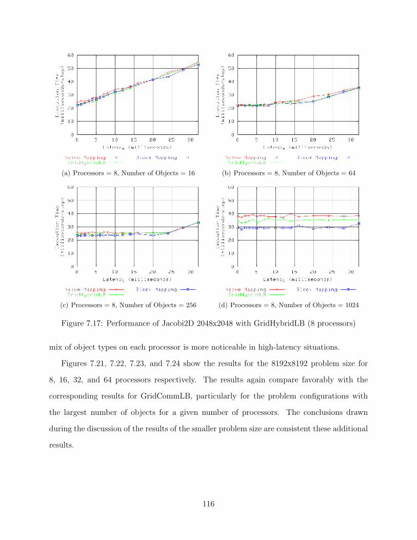
(a) Processors = 8, Number of Objects = 16 (b) Processors = 8, Number of Objects = 64
(c) Processors = 8, Number of Objects = 256 (d) Processors = 8, Number of Objects = 1024
Figure 7.17: Performance of Jacobi2D 2048x2048 with GridHybridLB (8 processors)
mix of object types on each processor is more noticeable in high-latency situations.
Figures 7.21, 7.22, 7.23, and 7.24 show the results for the 8192x8192 problem size for
8, 16, 32, and 64 processors respectively. The results again compare favorably with the
corresponding results for GridCommLB, particularly for the problem configurations with
the largest number of objects for a given number of processors. The conclusions drawn
during the discussion of the results of the smaller problem size are consistent these additional
results.
116

(a) Processors = 16, Number of Objects = 16 (b) Processors = 16, Number of Objects = 64
(c) Processors = 16, Number of Objects = 256 (d) Processors = 16, Number of Objects = 1024
Figure 7.18: Performance of Jacobi2D 2048x2048 with GridHybridLB (16 processors)
117

(a) Processors = 32, Number of Objects = 64 (b) Processors = 32, Number of Objects = 256
(c) Processors = 32, Number of Objects = 1024 (d) Processors = 32, Number of Objects = 4096
Figure 7.19: Performance of Jacobi2D 2048x2048 with GridHybridLB (32 processors)
118

(a) Processors = 64, Number of Objects = 64 (b) Processors = 64, Number of Objects = 256
(c) Processors = 64, Number of Objects = 1024 (d) Processors = 64, Number of Objects = 4096
Figure 7.20: Performance of Jacobi2D 2048x2048 with GridHybridLB (64 processors)
119

(a) Processors = 8, Number of Objects = 16 (b) Processors = 8, Number of Objects = 64
(c) Processors = 8, Number of Objects = 256 (d) Processors = 8, Number of Objects = 1024
Figure 7.21: Performance of Jacobi2D 8192x8192 with GridHybridLB (8 processors)
120
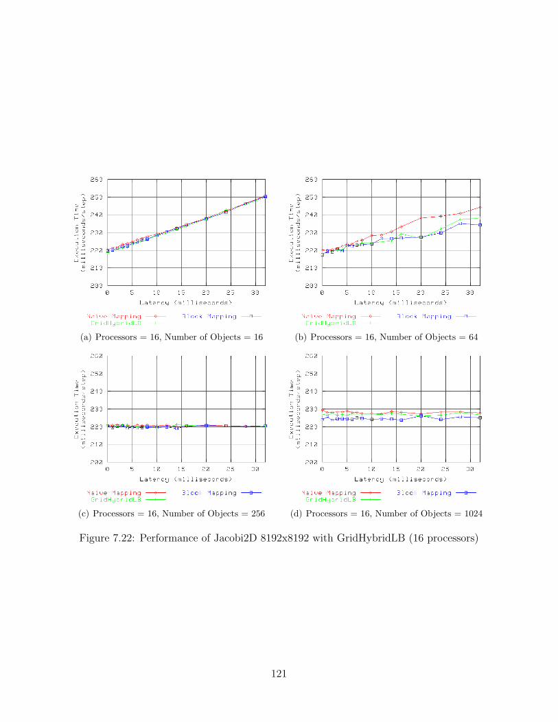
(a) Processors = 16, Number of Objects = 16 (b) Processors = 16, Number of Objects = 64
(c) Processors = 16, Number of Objects = 256 (d) Processors = 16, Number of Objects = 1024
Figure 7.22: Performance of Jacobi2D 8192x8192 with GridHybridLB (16 processors)
121

(a) Processors = 32, Number of Objects = 64 (b) Processors = 32, Number of Objects = 256
(c) Processors = 32, Number of Objects = 1024 (d) Processors = 32, Number of Objects = 4096
Figure 7.23: Performance of Jacobi2D 8192x8192 with GridHybridLB (32 processors)
122
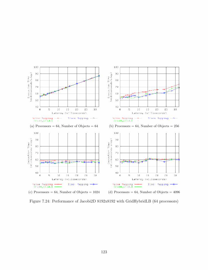
(a) Processors = 64, Number of Objects = 64 (b) Processors = 64, Number of Objects = 256
(c) Processors = 64, Number of Objects = 1024 (d) Processors = 64, Number of Objects = 4096
Figure 7.24: Performance of Jacobi2D 8192x8192 with GridHybridLB (64 processors)
123
7.3.4 Overhead
The first phase of load balancing with GridHybridLB uses Metis to partition objects onto
clusters. The computational complexity of this phase matches that of GridMetisLB. If the
second phase of load balancing uses the simpler object placement method employed by
GridCommLB, then the asymptotic upper bound of the overall load balancing operation is
dominated by the time spent in the first phase. Alternatively, if the second phase of load
balancing uses the more complex seed technique, the time spent in the second phase of the
algorithm becomes the upper bound. For a computation with n objects, n passes must be
made through an O(n2) algorithm that first locates the objects that are mapped to a given
processor and then the objects that neighbor each mapped object, so the overall complexity
is O(n3). Maintaining a heap data structure for each object containing neighboring objects
would allow the seed technique running time complexity to be reduced to O(n∗ log(n)), and
this means that the overall running time complexity of balancing would be dominated by
the time spent partitioning the communication graph in the first phase.
Table 7.3 shows the amount of time required to balance the Jacobi2D examples shown in
the previous section. The results for 4096 objects clearly show the effects of the inefficient
algorithm used to implement the seed technique in the second phase of load balancing.
Correcting this is an important item of future work.
7.3.5 Limitations
GridHybridLB is probably the generally best Grid topology-aware load balancer developed in
this thesis since it is effective at reducing the volume of cross-cluster traffic as well as effective
at balancing the objects assigned to each cluster. The biggest limitation of the load balancer
is the fact that the initial graph partitioning phase of the algorithm is computationally
expensive. Unfortunately, all objects in the computation must be considered to carry out
this phase correctly since it is the first task the load balancer must perform. That is, it
124

Number of Number of Strategy Time Load Balancing TimeProcessors Objects (seconds) (seconds)
8 16 0.000499 0.1473218 64 0.000965 0.1451948 256 0.014053 0.1607578 1024 0.781349 0.94704116 16 0.000504 0.08785516 64 0.001029 0.09409916 256 0.009317 0.21185416 1024 0.425668 0.59499532 64 0.000817 0.05767032 256 0.006251 0.07119932 1024 0.238152 0.33283832 4096 6.667677 6.84887464 64 0.000799 0.05388064 256 0.005090 0.04901164 1024 0.146505 0.20245364 4096 6.880359 7.093415
Table 7.3: Overhead of the hybrid load balancing technique in GridHybridLB
seems that there is no clever way to optimize the load balancer by ignoring some objects
during this phase. This seems to suggest that solutions like ParMetis are necessary for large
computations.
7.4 Summary
This chapter has introduced techniques for improving the performance of tightly-coupled
parallel applications running in Grid computing environments by load balancing. The tech-
niques differ from other approaches used by Charm++ load balancers because they take into
consideration details of the Grid environment topology in addition to characteristics of the
application such as the measured CPU load or messages sent in the objects that make up the
computation. The techniques in this chapter are best suited for situations in which the total
number of objects in the computation is large enough that an adjustment in the mapping of
objects to processors can produce an observable improvement in performance. In practice,
125

these situations are probably more likely to be found in realistic applications than the more
constrained situations where the object prioritization technique of the previous chapter is
applicable.
The three load balancing techniques developed in this chapter involve tradeoffs that make
each technique suitable for use in certain circumstances. GridCommLB is best used to bal-
ance applications in which objects do not need to migrate across cluster boundaries since
this balancer lacks this capability. For example, a common practice in structural dynam-
ics problems that involve irregularly-shaped objects is to overlay “patches” of structured
meshes over the object rather than using a single computationally-expensive irregular mesh.
These patches could manually be assigned to clusters in a Grid environment by placing one
or more patches on each cluster. In this scenario, communication between clusters corre-
sponds directly to communication between patches in the problem. Because the structure of
the problem starts out mostly balanced through manual effort, a Grid topology-aware load
balancer can most likely best improve application performance simply by ensuring that the
border objects and local-only objects in each cluster are spread evenly among the processors
in the cluster while simultaneously maintaining balanced CPU utilization. GridCommLB
does exactly this without paying the overhead of considering object migrations across clus-
ter boundaries, which are probably not necessary in this problem. In many other problems,
however, migrating objects across cluster boundaries is important for establishing good ap-
plication performance. In these situations, GridMetisLB or GridHybridLB are much better
choices for load balancing. In cases where an application is expected to be well within
a latency-tolerated regime, such as when cross-site latencies are less than the application
per-step time, GridMetisLB is probably the best choice of load balancer. This is because
GridMetisLB likely creates a more favorable volume of communication inside each cluster
than GridHybridLB can, at the expense of not as evenly spreading the border objects and
local-only objects among the processors in each cluster. In cases where the application is
operating beyond complete latency tolerance, GridHybridLB is likely to give better results
126
due to its ability to enhance the latency masking capabilities of the Charm++ runtime sys-
tem by evenly distributing border objects and local-only objects across the processors in
each cluster. Finally, because GridHybridLB combines the best features of GridCommLB
and GridMetisLB into a load balancer that optimizes the wide-area communication of an
application as well as producing a good balance of objects within each cluster, it is probably
the best choice for situations in which the structure of an application is not well understood.
127
Chapter 8
Case Studies
The discussion in Chapter 4 introduces the use of message-driven objects as a technique for
masking the effects of latency in tightly-coupled parallel applications running in Grid com-
puting environments. This is the primary architectural contribution of this thesis. Chapter 5
demonstrates that the latency masking capabilities of the Charm++ runtime system may be
enhanced by (manually) mapping objects to processors such that each processor holds a rel-
atively small number of border objects and a relatively large number of local-only objects.
Chapters 6 and 7 present automated techniques that act as optimizations to the latency
masking capabilities of message-driven execution, improving application performance par-
ticularly when cross-site latency begins to increase. Throughout these four chapters, the
techniques are illustrated through the running example of a simple five-point stencil bench-
mark (Jacobi2D). The primary advantage of using a simple benchmark to illustrate these
techniques is that it is easy to understand the benchmark in its entirety and reason about the
effects of each particular technique on the benchmark’s performance. However, Jacobi2D
is in many ways not representative of practical scientific applications. For example, the
benchmark is very symmetrical in its structure, and this results in all objects throughout
the benchmark having identical characteristics such as measured CPU load and number of
messages sent.
This chapter presents two case studies in which the techniques of the thesis are employed
to optimize practical scientific applications. These studies give some perspective on the
feasibility of deploying typical tightly-coupled parallel applications in real Grid computing
environments through the use of techniques presented in this thesis.
128
8.1 Experiment Environments
The case study applications are examined in two environments: an artificial latency en-
vironment used for the experiments in the previous chapters and a real Grid computing
environment consisting of clusters at three high-performance computing centers. This sec-
tion describes details of these two environments.
8.1.1 Artificial Latency Environment
The examples in Chapters 4 through 7, as well as the case studies in the current chapter, are
studied in an artificial latency environment described in Section 2.4. In this environment,
the application being examined is run on real machines using a system software stack that
is nearly identical to that used to run the application in an actual Grid environment. The
only difference between the system software stack used in the artificial latency environment
and that used in a real Grid environment is the introduction of a “delay device” driver in the
Virtual Machine Interface (VMI) message layer to inject specified latencies in the message
paths between arbitrary pairs of nodes. Thus, machines from a single real cluster can be used
to very accurately simulate a Grid computing environment for the purposes of conducting
the experiments in this thesis.
A disadvantage of the artificial latency environment is that it requires access to the type
and number of computational resources for which results are to be obtained. This differs from
experiments run in some type of simulation environment, where the simulator may run on
machines that are entirely different from the machines that are being simulated. A distinct
advantage of the artificial latency environment, however, is that results obtained using this
environment match the results obtained in a real Grid environment very closely. Some
of the effects of the optimizations described in this thesis (e.g., the technique described in
Chapter 6) are quite subtle, so it is important that the experiments be run in an environment
that is as close to a real Grid environment as possible in order to be able to draw conclusions
129

from these results.
The artificial latency environment used for all experiments in this thesis consists of dual-
processor 1.5 GHz Intel Itanium 2 compute nodes in the TeraGrid cluster Mercury, located
at the National Center for Supercomputing Applications [1]. Each dual-processor node has
4 gigabytes of memory. Nodes within each simulated cluster communicate with each other
via a high-performance Myrinet, while messages that pass between simulated clusters are
sent via TCP/IP over Gigabit Ethernet (in addition to being intercepted, and delayed, by
the VMI delay device driver).
8.1.2 TeraGrid Environment
To validate the results obtained in the artificial latency environment described above, the
case study experiments were also run in a real Grid computing environment consisting of
clusters from three TeraGrid sites at the National Center for Supercomputing Applications
(NCSA) in Urbana, Illinois; Argonne National Laboratory (ANL) in Chicago, Illinois; and
the San Diego Supercomputer Center (SDSC) in San Diego, California. These sites are
shown on the map in Figure 1.2.
The topology of the wide-area network connecting the three TeraGrid sites used for
experiments consists of a forty-gigabit-per-second optical trunk, made up of four ten-gigabit-
per-second lines, connecting a Chicago hub to a Los Angeles hub. Both NCSA and ANL
connect to the Chicago hub via a thirty-gigabit-per-second (three ten-gigabit-per-second)
connection while SDSC connects to the Los Angeles hub via a similar thirty-gigabit-per-
second connection. Cross-site latency, not bandwidth, is generally the limiting factor for
distributed applications running in this environment. One-way latencies were measured
using ICMP Ping between NCSA and ANL as 1.7 milliseconds, between ANL and SDSC as
29.1 milliseconds, and between NCSA and SDSC as 30.1 milliseconds. For all experiments
used in this thesis, comparisons can be made to the results recorded for artificial latencies
of 2 milliseconds and 32 milliseconds.
130

The compute nodes used for all cross-site experiments in this chapter match those used
in the artificial latency environment described above (dual-processor 1.5 GHz nodes with
4 gigabytes memory each). Within each cluster, nodes communicate with each other via a
high-performance Myrinet network. Communication across clusters is via TCP/IP over the
trunked wide-area TeraGrid network. VMI is used as the underlying messaging layer, and
in the case of the real TeraGrid, the VMI delay device is removed from the communication
stack.
8.2 Molecular Dynamics
The first case study application considered in this chapter is a classical molecular dynam-
ics application. Molecular dynamics is a form of computer simulation that examines the
behavior of biomolecular systems. In these simulations, atoms and molecules are allowed
to interact for a period of time under known laws of physics. The computational complex-
ity of such simulations is usually quite extreme, and thus the use of parallel computing is
important. Due to its message-driven object style of problem decomposition, Charm++ is
well-suited for developing molecular dynamics software.
8.2.1 LeanMD
The molecular dynamics application used for the experiments in this thesis is LeanMD [37].
LeanMD is implemented as a framework for parallel molecular dynamics simulations and
provides a core parallelization infrastructure along with input and output routines for reading
and writing simulation data. It serves as a simpler version of NAMD [45], a production-
quality application used by biophysicists around the world, allowing easy experimentation
and scaling to extremely large petascale-sized machines.
Molecular dynamics codes typically employ a spatial decomposition style in which the
atoms of a biomolecular system, composed of proteins, cell membranes, SNA, and waters,
131
interact with the other atoms that are within a certain cutoff distance. Each timestep
involves calculating the forces acting on all atoms and then using these forces to update the
positions and velocities of each atom.
Within LeanMD, all computation takes place within a simulation box, a bounding box
for all atoms involved in the simulation. The space within a simulation box is divided into
regular cubic regions of simulation space called cells. Each cell is responsible for all the
atoms that fall within its boundary, their coordinates, and the forces exerted on them. As
described above, molecular dynamics simulations involve the interaction of atoms with other
atoms within a certain cutoff distance. In a simulation with a k-away cutoff distance, a cubic
region of simulation space formed by (2k + 1)3 cells is considered.
Electrostatic and van der Waals interactions between every pair of neighboring cells are
computed by a separate cell-pair object. These interactions constitute the bulk of processor
time used by the application, although there are other force computations involving bonds
between atoms. In each time-step, each cell “integrates” all forces on its atoms and changes
their positions based on new acceleration and velocities calculated. It then multicasts its
atoms’ coordinates to the 26 cell-pairs (three-dimensional region of 3 × 3 × 3) that depend
on it. Each cell pair calculates forces on the two sets of atoms it receives, and sends them
back to the two cells.
For the simulation used in this thesis, it is important to note that the computation in
each cell pair depends on messages from at most two other objects, possibly on two different
processors. Thus, in the benchmark used here, there are 216 cells and 3,024 cell pairs
(k = 1). On each processor, there may be several tens of cell-pair objects. In a multi-cluster
context, some subset of these objects (“subset A”) require messages from cells within their
own cluster, while a different subset (“subset B”) may require one or both messages from
outside the cluster. As a result, a processor is able to execute objects in subset A while
waiting for high-latency messages for objects in subset B from another cluster. This renders
the application latency tolerant to some extent.
132

(a) Processors = 16 (b) Processors = 32
(c) Processors = 64 (d) Processors = 128
Figure 8.1: Performance of LeanMD
8.2.2 Performance in Artificial Latency Environment
Figure 8.1 shows the performance of LeanMD for 16, 32, 64, and 128 processors running in
the artificial latency environment with cross-cluster latencies ranging from 8 milliseconds to
128 milliseconds. As before, the application is partitioned between two clusters, with half
the processors in one cluster and half the processors in the second cluster. For example, the
16 processor experiment is executed with 8 processors in the first cluster and 8 processors
in the second cluster.
Results are shown for the application running without load balancing, as well as with
the basic Grid communications load balancer (GridCommLB), the graph partitioning load
133

balancer (GridMetisLB), and the hybrid load balancer (GridHybridLB) described in Chap-
ter 7. As an additional point of reference, results are also shown for GreedyLB, a load
balancer that adjusts object mapping based on measured CPU load to ensure that each pro-
cessor has the same amount of computation work. GreedyLB makes no consideration to the
communication properties of each object. GreedyLB is known to produce good results with
LeanMD [37], and is important for achieving good scalability with the application beyond
32 processors.
Figure 8.1(a) shows the results for 16 processors. The results here are mostly unremark-
able except to note that the results without load balancing show a per-step execution time of
approximately 1000 milliseconds per timestep, while the results for all load balancers show
approximately a 10% improvement in performance with a per-step execution time of ap-
proximately 900 milliseconds per timestep. The horizontal lines on the graph for each set of
results indicate that the effects of cross-site latency have no impact on the per-step execution
time of the application. That is, for 16 processors, the application gets the same performance
running in a Grid environment consisting of two clusters separated by 128 milliseconds of
latency as it gets running entirely within a single cluster.
Figure 8.1(b) shows the results for 32 processors. Scalability of the results without load
balancing is reasonable; doubling the number of processors results in a per-step execution
time that is roughly half of the previous results (approximately 550 milliseconds per timestep
with 32 processors versus approximately 1000 milliseconds per timestep with 16 processors).
Again, the results for all load balancers show good improvements over the results without
load balancing, and all load balancers give somewhat similar results. However, the results for
GreedyLB and GridCommLB seem to be more on par with each other while GridMetisLB
and GridHybridLB seem to give slightly better results, particularly as cross-cluster latencies
increase. This is not entirely unexpected. The algorithm used by GridCommLB does nothing
to reduce the volume of cross-cluster communication and only balances the objects in terms of
their measured CPU loads while simultaneously spreading the border objects evenly among
134

the processors in each cluster. This resembles the strategy employed by GreedyLB, except
GreedyLB does not take each object’s communication characteristics into consideration when
making load balancing decisions. It is likely that this explains the results for these two load
balancers on the right-most three data points (96, 112, and 128 milliseconds of latency). For
these three data points, the results for GridCommLB outperform those of GreedyLB. Both
sets of results show a slight upward trend here, indicating that the effects or cross-cluster
latency are not entirely being masked, but evenly distributing the border objects and local-
only objects among each cluster’s processors in the GridCommLB case allows a small degree
of improved latency masking. Better performance, however, is evident in the results for
GridMetisLB and GridHybridLB which remain clearly horizontal through 128 milliseconds
of latency.
Figure 8.1(c) shows the results for 64 processors. The results without load balancing
show an extreme lack of scalability with this doubling of the number of processors. It is
interesting to observe the right-most three data points here show a slight upward trend in
the per-step execution time of the application. The per-step time of the unbalanced appli-
cation is around 425 milliseconds per step, and this is similar to the per-step time of the
GreedyLB and GridCommLB results for 32 processors above where the three right-most
data points show an upward trend. The most interesting results here are those for the
four load balancers. Load balancing in terms of measured CPU load makes a significant
improvement in per-step execution time (425 milliseconds per-step unbalanced improves to
225 milliseconds per-step balanced). As the cross-site latency increases, however, the results
for both GreedyLB and GridCommLB begin to show an upward trend in execution time
somewhere around 48 milliseconds of latency. The results for GridMetisLB and GridHy-
bridLB are especially promising, though, in that they remain nearly horizontal through 64
milliseconds of latency. Additionally, the results for GridMetisLB and GridHybridLB are
markedly better than those for the other two load balancers through 128 milliseconds of
latency. This is likely due to partitioning the object communication graph to reduce the
135
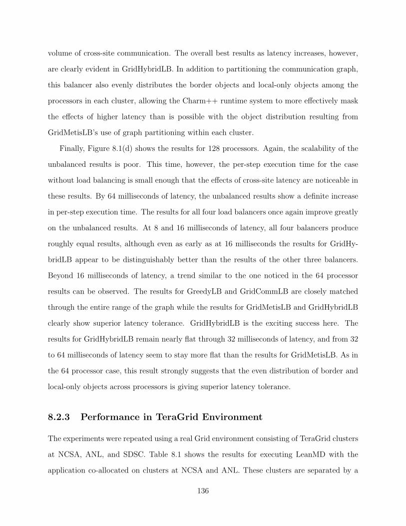
volume of cross-site communication. The overall best results as latency increases, however,
are clearly evident in GridHybridLB. In addition to partitioning the communication graph,
this balancer also evenly distributes the border objects and local-only objects among the
processors in each cluster, allowing the Charm++ runtime system to more effectively mask
the effects of higher latency than is possible with the object distribution resulting from
GridMetisLB’s use of graph partitioning within each cluster.
Finally, Figure 8.1(d) shows the results for 128 processors. Again, the scalability of the
unbalanced results is poor. This time, however, the per-step execution time for the case
without load balancing is small enough that the effects of cross-site latency are noticeable in
these results. By 64 milliseconds of latency, the unbalanced results show a definite increase
in per-step execution time. The results for all four load balancers once again improve greatly
on the unbalanced results. At 8 and 16 milliseconds of latency, all four balancers produce
roughly equal results, although even as early as at 16 milliseconds the results for GridHy-
bridLB appear to be distinguishably better than the results of the other three balancers.
Beyond 16 milliseconds of latency, a trend similar to the one noticed in the 64 processor
results can be observed. The results for GreedyLB and GridCommLB are closely matched
through the entire range of the graph while the results for GridMetisLB and GridHybridLB
clearly show superior latency tolerance. GridHybridLB is the exciting success here. The
results for GridHybridLB remain nearly flat through 32 milliseconds of latency, and from 32
to 64 milliseconds of latency seem to stay more flat than the results for GridMetisLB. As in
the 64 processor case, this result strongly suggests that the even distribution of border and
local-only objects across processors is giving superior latency tolerance.
8.2.3 Performance in TeraGrid Environment
The experiments were repeated using a real Grid environment consisting of TeraGrid clusters
at NCSA, ANL, and SDSC. Table 8.1 shows the results for executing LeanMD with the
application co-allocated on clusters at NCSA and ANL. These clusters are separated by a
136

Number of Execution Time Execution TimeProcessors Load Balancer (Artificial Latency) (TeraGrid)
16 No Load Balancing 985.957 1000.39716 GreedyLB 896.084 897.29716 GridCommLB 924.732 927.96016 GridMetisLB 899.336 913.68116 GridHybridLB 890.645 910.14132 No Load Balancing 546.597 532.96032 GreedyLB 464.077 456.13732 GridCommLB 470.128 470.74332 GridMetisLB 447.77 454.39932 GridHybridLB 451.448 463.29564 No Load Balancing 439.826 429.91564 GreedyLB 233.828 270.27164 GridCommLB 246.077 254.54164 GridMetisLB 227.421 256.47964 GridHybridLB 235.782 233.138128 No Load Balancing 227.506 229.904128 GreedyLB 119.736 135.841128 GridCommLB 123.477 145.163128 GridMetisLB 120.212 130.401128 GridHybridLB 119.21 119.918
Table 8.1: Performance comparison of LeanMD in artificial latency environment and Tera-Grid environment (NCSA-ANL)
latency of approximately 1.7 milliseconds. The results are compared to artificial latency
results collected for 2 milliseconds of latency. The results for the real Grid environment
match closely to the results for the artificial latency environment. This is expected, due to
the close similarities between the hardware and system software stacks used to collect both
sets of results.
Table 8.2 shows the results for executing LeanMD with the application co-allocated on
clusters at NCSA and SDSC. These clusters are separated by a latency of approximately
30.1 milliseconds. The results are compared to artificial latency results collected for 32
milliseconds of latency. As above, the results for the real Grid environment closely match
the results for the artificial latency environment.
137
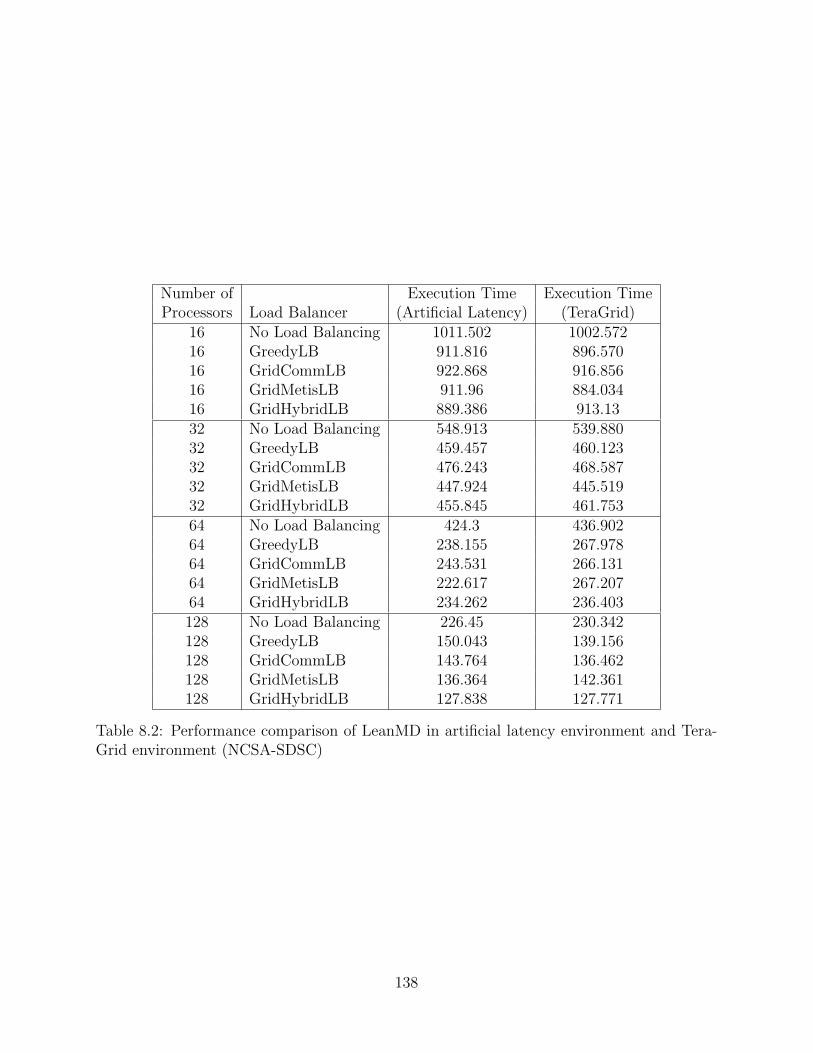
Number of Execution Time Execution TimeProcessors Load Balancer (Artificial Latency) (TeraGrid)
16 No Load Balancing 1011.502 1002.57216 GreedyLB 911.816 896.57016 GridCommLB 922.868 916.85616 GridMetisLB 911.96 884.03416 GridHybridLB 889.386 913.1332 No Load Balancing 548.913 539.88032 GreedyLB 459.457 460.12332 GridCommLB 476.243 468.58732 GridMetisLB 447.924 445.51932 GridHybridLB 455.845 461.75364 No Load Balancing 424.3 436.90264 GreedyLB 238.155 267.97864 GridCommLB 243.531 266.13164 GridMetisLB 222.617 267.20764 GridHybridLB 234.262 236.403128 No Load Balancing 226.45 230.342128 GreedyLB 150.043 139.156128 GridCommLB 143.764 136.462128 GridMetisLB 136.364 142.361128 GridHybridLB 127.838 127.771
Table 8.2: Performance comparison of LeanMD in artificial latency environment and Tera-Grid environment (NCSA-SDSC)
138

8.3 Finite Element Analysis of an Unstructured Mesh
The second case study application considered in this chapter is a Finite Element Analysis
code. Finite Element Analysis is commonly used to determine stresses and displacements in
mechanical objects and systems. Finite Element Analysis is used to find approximate solu-
tions to complex systems for which closed-form analytical solutions are difficult or impossible
to find.
Finite Element Analysis uses a numerical technique called the Finite Element Method
(FEM) in which a structure to be studied is divided into an unstructured mesh consisting
of triangles (2D) or tetrahedrons (3D). The mesh discretizes the continuous domain of the
structure into a set of discrete sub-domains that can be solved independently. Thus, the
FEM is a natural fit for solving on parallel computers. An attractive characteristic of the
FEM is that it can be applied easily to problems with irregular geometries and to problems
in which anomalies are present (e.g., a crack that propagates through a solid structure).
A computational challenge to parallel solutions of these types of situations is that load
imbalances are frequently encountered. Due to its dynamic nature, the Charm++ runtime
system can be leveraged for efficiently implementing solutions to irregular FEM problems.
8.3.1 Fractography3D
The Finite Element Method application used for the experiments in this thesis is called
Fractography3D [56]. Fractography3D is a software application for simulating the sponta-
neous initiation and propagation of a crack through a solid structure. Fractography3D takes
advantage of the FEM implementation provided by ParFUM [35], a parallel framework for
unstructured meshes. ParFUM handles the details of decomposing the problem in parallel
by laying a mesh over the structure to be studied, partitioning the mesh across the proces-
sors allocated to the computation, and defining shared “ghost zone” cells that exist along
partition boundaries. ParFUM itself is written as an MPI application that takes advantage
139

of the dynamic nature of the Adaptive MPI runtime system.
The particular problem used for the experiments here involves a fracture propagating
through a solid structure with dimensions of five meters wide, five meters high, and one
meter thick. This problem is configured to use 1000 AMPI virtual processors, and this
configuration is fixed and independent of the number of physical processors used to run the
application. Thus, increasing the number of physical processors results in each processor
having a smaller number of virtual processors mapped to it.
The Fractography3D application execution progresses in discrete timesteps. Due to the
dynamic nature of the problem being studied, each timestep can vary in duration from other
timesteps. Further, a given timestep may take a significantly different amount of time on two
different processors in the computation because some processors can have significantly more
work to do than other processors. In order to produce measurable and reproducible results
for this thesis, the Fractography3D application was modified to take a global barrier after
every 100 timesteps of execution. Further, a load balancing step was inserted at timestep
500. Finally, an average per-step execution time for the application was recorded for the
time taken to execute the application between timesteps 600 to 700. This configuration gives
the application enough time to properly start up and provide the Charm++ load balancing
framework with sufficient execution history to make a good load balancing decision. After
this load balancing adjustment, the application has enough time to fall into somewhat regular
execution. Even here, however, the average per-step time for each 100-timestep period can
still vary. To normalize against this, each run of the application was restarted from the
beginning, and its average per-step execution was recorded at timestep 700. These results
were found to vary little from run to run.
8.3.2 Performance in Artificial Latency Environment
Figure 8.2 shows the performance of Fractography3D for 8, 16, 32, and 64 processors running
in the artificial latency environment with cross-cluster latencies ranging from 8 milliseconds
140
to 128 milliseconds. As before, the application is partitioned between two clusters, with half
the processors in one cluster and half the processors in the second cluster. For example, the
8 processor experiment is executed with 4 processors in the first cluster and 4 processors in
the second cluster.
The results here are mostly unremarkable. The average per-step execution time of the
application is horizontal on all four graphs, indicating that the application performance in
a Grid environment, even when the clusters are separated by as much as 128 milliseconds of
latency, is on par with the application performance for a single cluster. This is not surprising
considering that the per-step execution time for the application running on 8 processors is
near 3000 milliseconds per step. Even with 64 processors and an average per-step execution
time of 375 to 400 milliseconds, the application has enough work to completely mask the
effects of cross-site latency. Load balancing in all four cases has little or no effect on the
application performance, however it is interesting to notice that the results for GridMetisLB
on 64 processors appear to be slightly worse than the results with no load balancing.
Figure 8.3 shows the performance of Fractography3D for 128 processors. In this figure,
the results without load balancing are flat through 64 milliseconds of latency, indicating that
the effects of cross-site latency are being entirely masked. After 64 milliseconds of latency,
the non-load balanced results show a linear upward slope, indicating that the application
transitions into a latency-dominated regime rather abruptly. The results for GreedyLB
closely follow the non-load balanced results, transitioning rapidly from latency tolerance to
latency-dominated near 64 milliseconds of latency. Both sets of results make sense due to
the fact that the communication pattern of Fractography3D is more complex than any of
the applications previously examined in this thesis, with each cell in the FEM depending on
up to six neighbors. Not optimizing the computation with respect to the Grid topology in
which the application is executing causes the effects of cross-cluster latency to have sudden
negative impacts on performance.
In the figure, it is very apparent that the results for GridMetisLB are significantly worse
141
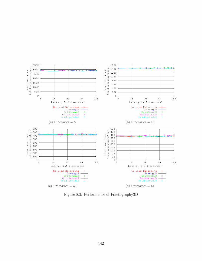
(a) Processors = 8 (b) Processors = 16
(c) Processors = 32 (d) Processors = 64
Figure 8.2: Performance of Fractography3D
142

than the results without load balancing. This is due to the fact that the use of graph
partitioning within each cluster does not guarantee that each processor will end up with a
balanced CPU utilization. At the beginning of the computation, the 1000 objects are evenly
distributed among the 128 processors, resulting in each processor holding 7 or 8 objects. Af-
ter load balancing with GridMetisLB, however, some processors hold as many as 10 objects
while others hold as few as 5 objects. That is, Metis places more emphasis on optimizing
the edge weights of the partitioned graph at the expense of having slightly unequal numbers
of objects within each partition (processor). In previous benchmarks and applications in
this thesis, this phenomenon has not been observed due to the fairly uniform nature of the
problems being studied. In this application, however, the non-uniform nature of the com-
munication causes this result. The other load balancers do not suffer from this difficulty
because they all specifically ensure that each processor is allocated an approximately-equal
amount of work, scaled to the processor’s relative performance compared to the other pro-
cessors in the same cluster, in addition to optimizing the communication characteristics of
the application.
The most interesting results in the figure are for GridCommLB and GridHybridLB.
Through 64 milliseconds of latency, the results of both balancers closely resemble the re-
sults without load balancing and for GreedyLB. However, after 64 milliseconds of latency,
GridCommLB and GridHybridLB significantly outperform the other results. The plots for
GridCommLB and GridHybridLB stay horizontal through at least 80 milliseconds of la-
tency. Even after this point, the slope of the line between 80 and 128 milliseconds of latency
is slightly less than linear. This indicates that the technique of spreading the border objects
and local-only objects evenly across processors gives the application improved latency tol-
erance compared to the mapping that results from GreedyLB that does not take the object
type into consideration. Further, because each processor in each cluster is guaranteed to be
balanced in terms of CPU utilization (scaled to the relative performance of each processor)
with the load balancing techniques employed by GridCommLB and GridHybridLB, the re-
143

Figure 8.3: Performance of Fractography3D on 128 processors
sults for these balancers cannot suffer the same decrease in performance as happens when
balancing the problem with GridMetisLB.
8.3.3 Performance in TeraGrid Environment
The experiments were repeated using a real Grid environment consisting of TeraGrid clusters
at NCSA, ANL, and SDSC. Table 8.1 shows the results for executing Fractography3D with
the application co-allocated on clusters at NCSA and ANL. These clusters are separated by
a latency of approximately 1.7 milliseconds. The results are compared to artificial latency
results collected for 2 milliseconds of latency. As in the case of LeanMD, the results for the
real Grid environment match closely to the results for the artificial latency environment.
Table 8.2 shows the results for executing Fractography3D with the application co-allocated
on clusters at NCSA and SDSC. These clusters are separated by a latency of approximately
30.1 milliseconds. The results are compared to artificial latency results collected for 32 mil-
144

Number of Execution Time Execution TimeProcessors Load Balancer (Artificial Latency) (TeraGrid)
8 No Load Balancing 2847.265 2851.4748 GreedyLB 2859.825 2852.8478 GridCommLB 2847.670 2845.9588 GridMetisLB 2876.524 2862.6268 GridHybridLB 2840.316 2838.33016 No Load Balancing 1437.385 1437.78216 GreedyLB 1451.436 1450.23816 GridCommLB 1433.360 1433.32316 GridMetisLB 1441.121 1439.64316 GridHybridLB 1444.560 1442.58932 No Load Balancing 726.742 727.14632 GreedyLB 736.830 734.77032 GridCommLB 741.093 740.04732 GridMetisLB 752.630 752.77932 GridHybridLB 736.955 736.03464 No Load Balancing 381.374 381.83864 GreedyLB 373.846 374.71164 GridCommLB 374.876 374.42664 GridMetisLB 392.551 390.05864 GridHybridLB 376.345 377.162128 No Load Balancing 191.708 190.991128 GreedyLB 187.513 188.295128 GridCommLB 188.076 188.594128 GridMetisLB 226.957 227.257128 GridHybridLB 187.392 187.272
Table 8.3: Performance comparison of Fractography3D in artificial latency environment andTeraGrid environment (NCSA-ANL)
145

Number of Execution Time Execution TimeProcessors Load Balancer (Artificial Latency) (TeraGrid)
8 No Load Balancing 2862.865 2863.2708 GreedyLB 2861.515 2856.8878 GridCommLB 2858.864 2857.2148 GridMetisLB 2853.903 2850.8938 GridHybridLB 2837.086 2832.54816 No Load Balancing 1429.286 1427.98616 GreedyLB 1448.782 1446.87816 GridCommLB 1443.447 1439.72616 GridMetisLB 1457.795 1458.32416 GridHybridLB 1444.868 1442.54232 No Load Balancing 725.611 722.74632 GreedyLB 744.435 743.34932 GridCommLB 736.320 737.58232 GridMetisLB 739.023 737.98232 GridHybridLB 739.158 737.12464 No Load Balancing 383.909 384.14764 GreedyLB 376.279 376.65764 GridCommLB 375.996 375.31064 GridMetisLB 393.945 394.17264 GridHybridLB 375.579 374.355128 No Load Balancing 193.056 194.311128 GreedyLB 190.248 191.009128 GridCommLB 189.657 191.350128 GridMetisLB 231.628 232.239128 GridHybridLB 188.871 189.298
Table 8.4: Performance comparison of Fractography3D in artificial latency environment andTeraGrid environment (NCSA-SDSC)
liseconds of latency. As above, the results for the real Grid environment closely match the
results for the artificial latency environment.
8.4 Summary
This chapter has presented two case studies in which the techniques developed in this thesis
are used to optimize practical scientific applications in both a simulated Grid environment
and in the national TeraGrid environment. Overall, the results of these experiments suggest
146

that rather than challenging the effectiveness of the thesis techniques for efficiently execut-
ing tightly-coupled parallel applications in Grid computing environments, the more complex
computations and communication structures of realistic scientific applications, compared to
the simpler Jacobi2D benchmark studied previously, are in fact a good match for the tech-
niques developed in this thesis. The basic latency masking capabilities of the Charm++
runtime system are immediately available to both native Charm++ applications (such as
LeanMD) and more traditional MPI applications (such as Fractography3D), and these capa-
bilities can be enhanced by the use of optimization techniques such as Grid topology-aware
load balancing that extend the latency masking capabilities into regions of greater cross-site
latencies.
These results are very encouraging because they strongly suggest that techniques devel-
oped at the runtime system level can be effective at allowing the efficient execution of tightly-
coupled parallel applications in Grid computing environments, and that these techniques can
be readily applied to applications that use a variety of common problem decomposition styles
without requiring modifications to the application software.
147

Chapter 9
Conclusion
This thesis has presented a toolbox of techniques that can be applied to the problem of
efficiently executing tightly-coupled parallel applications in Grid computing environments.
The primary architectural contribution of the thesis is the use of message-driven objects at
the runtime system (middleware) level to mask the effects of cross-site latency on an appli-
cation that is co-allocated across clusters at multiple geographically-distributed Grid sites.
By performing useful work in ready objects during the otherwise-wasted time required for
messages to travel across a high-latency wide-area network, a tightly-coupled parallel appli-
cation can achieve performance in a Grid environment that is on par with its performance
in a single cluster.
The thesis also develops optimization techniques that enhance the performance of the
message-driven object architecture. One optimization technique is object prioritization. By
tuning the runtime system’s object scheduler to prioritize the execution of border objects,
which communicate with neighbors on remote clusters, over the execution of local-only ob-
jects, which communicate only with neighbors within the local cluster, execution within each
application timestep is adjusted such that the border objects occur nearer to the beginning
of the timestep. This gives more opportunities to overlap the high-latency cross-site mes-
sages sent by the border objects with work driven in local-only objects and improves overall
application performance. This technique is generally only suited for situations in which the
number of objects on each processor is somewhat limited, resulting in the runtime system
being able to somewhat, but not entirely, mask the effects of cross-site latency.
With a greater number of objects on each processor, the second optimization technique,
148

Grid topology-aware load balancing, becomes effective. This technique takes into consider-
ation characteristics of the objects that make up the computation, including such things as
measured CPU load and communication characteristics, and couples this information with
knowledge of the topology of the Grid environment itself in order to make dynamic adjust-
ments to the mapping of objects to processors. Three sub-techniques are used here. The
first, and simplest, balances objects based on their measured CPU loads and additionally
organizes the objects in each cluster such that the border objects and local-only objects
are spread as evenly across the processors in each cluster as possible. This hopefully gives
each processor a favorable mixture of border objects and local-only objects which can be
used to mask cross-site latency. The second load balancing technique is more complex and
takes into consideration the relationship between pairs of objects in a computation by using
graph partitioning algorithms in an attempt to reduce the volume of cross-cluster commu-
nication as well as the volume of communication internal to each cluster. Finally, the third
load balancing technique combines the best features of the first two techniques, employing
graph partitioning algorithms at the wide-area level and simpler object balancing within
each cluster, to create a hybrid technique that delivers all-around good results.
The primary research question posed at the beginning of the research in this thesis is
whether it is feasible to deploy tightly-coupled parallel applications representative of realistic
scientific workloads in Grid computing environments. To demonstrate this, two case studies
were undertaken to examine the Grid deployment of two tightly-coupled parallel applications
from the fields of molecular dynamics and structural dynamics. These case study applications
are representative of realistic scientific workloads. The results of the case study experiments
strongly suggest that it is indeed feasible to deploy tightly-coupled applications in Grid
computing environments and expect to achieve application performance levels that are on
par with the performance of the application executing within a single cluster.
It has been observed that many modern high-performance computing environments, such
as clusters of SMPs, represent a hierarchy of communication interconnects [36]. Grid comput-
149
ing environments are no exceptions to this observation, however Grid environments present
one significant challenge that is not present in other environments: characteristics of a Grid
environment can change during the execution of a job. To that end, it seems likely that
successful Grid runtime systems and middleware must employ dynamic techniques that can
optimize an application’s performance during execution based on measurements collected
both about the application and about the Grid environment itself. The rich features of
the Charm++ and Adaptive MPI systems make them ideal candidates for Grid work, and
this may be in contrast to simpler and somewhat more static runtime systems that support
languages such as Titanium [54].
Recent trends suggest a growing interest in deploying realistic scientific applications in
Grid computing environments. For example, a technology demonstration at the SC05 con-
ference held in November 2005 in Seattle, Washington linked the United States TeraGrid
and the UK National Grid Service via a transatlantic fiber connection to conduct interac-
tive simulations in three large-scale applications [7]. These applications were NEKTAR, a
simulation of blood flow in the human arterial tree using fluid dynamics (led by George
Karniadakis at Brown University); SPICE (Simulated Pore Interactive Computing Environ-
ment), studying translocation of nucleic acids across membrane channel pores in biological
cells (led by Peter Coveney at University of London); and VORTONICS, a vortex dynamics
simulation using 3D Navier-Stokes computations (led by Bruce Boghosian at Tufts Uni-
versity). Overall, the techniques presented in this thesis may offer interesting possibilities
for leveraging Grid computing resources on an ad-hoc basis for applications such as these.
Two of the techniques, the primary message-driven architectural technique and the Grid
topology-aware load balancing technique using graph partitioning, have been particularly
well received by Grid computing practitioners [32, 33]. Additionally, independent research
conducted by Ragu Reddy and David C. O’Neal at the Pittsburg Supercomputing Center
and presented at the 2006 TeraGrid Conference in Indianapolis, Indiana [46] reproduces the
findings of Chapter 4 of this thesis.
150

References
[1] TeraGrid project homepage. http://www.teragrid.org/.
[2] Connection Machine model CM-2 technical summary. Technical report, Thinking Ma-chines Corporation, 1990.
[3] Gabrielle Allen, Thomas Dramlitsch, Ian Foster, Nicholas T. Karonis, Matei Ripeanu,Edward Seidel, and Brian Toonen. Supporting efficient execution in heterogeneousdistributed computing environments with Cactus and Globus. In Proceedings of SC2001,November 2001.
[4] Olivier Aumage and Guillaume Mercier. MPICH/MADIII: A cluster of clusters en-abled MPI implementation. In Proceedings of 3rd International Symposium on ClusterComputing and the Grid, May 2003.
[5] S. Baden, P. Colella, D. Shalit, and B. Van Straalen. Abstract KeLP. In 10th SIAMConference on Parallel Processing for Scientific Computing, March 2001.
[6] N. J. Boden, D. Cohen, R. E. Felderman, A. E. Kulawik, C. L. Seitz, J. N. Seizovic, andWen-King K. Su. Myrinet — A gigabit-per-second local-area-network. IEEE Micro,15(1):29–36, February 1995.
[7] Bruce Boghosian, Peter Coveney, Suchuan Dong, Lucas Finn, Shantenu Jha, GeorgeKarniadakis, and Nicholas Karonis. NEKTAR, SPICE and Vortonics: Using federatedgrids for large scale scientific applications. Cluster Computing, 10(3):351–364, 2007.
[8] Chris Ding and Yun He. A ghost cell expansion method for reducing communicationsin solving PDE problems. In Proceedings of SC2001, November 2001.
[9] Menno Dobber, Ger Koole, and Rob van der Mei. Dynamic load balancing experimentsin a grid. In Proceedings of the 5th International Symposium on Cluster Computing andthe Grid, pages 1063–1070. IEEE Computer Society, 2005.
[10] Ian Foster and Carl Kesselman. The Globus toolkit. In Ian Foster and Carl Kessel-man, editors, The Grid: Blueprint for a New Computing Infrastructure, pages 259–278.Morgan-Kaufmann, San Francisco, CA, July 1999.
[11] Ian Foster and Carl Kesselman, editors. The Grid: Blueprint for a Future ComputingInfrastructure. Morgan-Kaufmann, San Francisco, CA, July 1999.
151

[12] Ian Foster and Carl Kesselman, editors. The Grid 2: Blueprint for a Future ComputingInfrastructure. Morgan-Kaufmann, San Francisco, CA, January 2004.
[13] Ian Foster, Carl Kesselman, and Steven Tuecke. Nexus: Runtime support for task-parallel programming languages. Technical Memo ANL/MCS-TM-205, Argonne Na-tional Laboratory, 1995.
[14] Ian Foster, Carl Kesselman, and Steven Tuecke. The Nexus approach to integratingmultithreading and communication. Journal of Parallel and Distributed Computing,37(1):70–82, August 1996.
[15] G. Fox, M. Johnson, G. Lyzenga, S. Otto, J. Salmon, and D. Walker. Solving Problemson Concurrent Processors, volume Volume I: General Techniques and Regular Problems.Prentice Hall, Englewood Cliffs, New Jersey, 1988.
[16] Andrew S. Grimshaw, Willaim A. Wulf, James C. French, Alfred C. Weaver, and PaulF. Reynolds Jr. Legion: The next logical step toward a nationwide virtual computer.Technical Report CS-94-21, University of Virginia Computer Science Department, June1994.
[17] Attila Gursoy. Simplified Expression of Message Driven Programs and Quantification ofTheir Impact on Performance. PhD thesis, University of Illinois at Urbana-Champaign,1994.
[18] Attila Gursoy and L.V. Kale. Performance and modularity benefits of message-drivenexecution. Journal of Parallel and Distributed Computing, 64:461–480, 2004.
[19] Bruce Hendrickson and Robert Leland. The Chaco user’s guide, ver-sion 2.0, technical report SAND94-2692, 1994. http://www.ti.com/corp/docs/press/backgrounder/omap.shtml.
[20] Chao Huang, Orion Lawlor, and L. V. Kale. Adaptive MPI. In Proceedings of the 16thInternational Workshop on Languages and Compilers for Parallel Computing, 2003.
[21] L. V. Kale and Sanjeev Krishnan. Charm++: Parallel programming with message-driven objects. In Gregory V. Wilson and Paul Lu, editors, Parallel Programming usingC++, pages 175–213. MIT Press, 1996.
[22] Laxmikant V. Kale. The virtualization model of parallel programming: Runtime opti-mizations and the state of art. In Proceedings of 2002 Los Alamos Computer ScienceInstitute, Albuquerque, NM, October 2002.
[23] L.V. Kale and Sanjeev Krishnan. Medium grained execution in concurrent object-oriented systems. In Workshop on Efficient Implementation of Concurrent Object Ori-ented Languages, at OOPSLA 1993, September 1993.
[24] Nicholas Karonis, Brian Toonen, and Ian Foster. MPICH-G2: A grid-enabled implemen-tation of the Message Passing Interface. Journal of Parallel and Distributed Computing,63(5):551–563, May 2003.
152
[25] George Karypis and Vipin Kumar. Analysis of multilevel graph partitioning. In Su-percomputing ’95: Proceedings of the 1995 ACM/IEEE conference on Supercomputing(CDROM), page 29, New York, NY, USA, 1995. ACM Press.
[26] George Karypis and Vipin Kumar. A fast and high quality multilevel scheme for parti-tioning irregular graphs. SIAM Journal of Scientific Computing, 20(1):359–392, 1998.
[27] George Karypis and Vipin Kumar. Metis: A Software Package for Partitioning Unstruc-tured Graphs, Partitioning Meshes, and Computing Fill-Reducing Orderings of SparseMatrices, September 1998.
[28] George Karypis and Vipin Kumar. Multilevel k-way partitioning scheme for irregulargraphs. Journal of Parallel and Distributed Computing, 48(1):96–129, 1998.
[29] George Karypis and Vipin Kumar. A parallel algorithm for multilevel graph partitioningand sparse matrix ordering. Journal of Parallel and Distributed Computing, 48(1):71–95,1998.
[30] James H. Kaufman, Glenn Deen, Toby J. Lehman, and John Thomas. Grid computingmade simple. The Industrial Physicist, August/September 2003.
[31] B. W. Kernighan and S. Lin. An efficient heuristic procedure for partitioning graphs.The Bell System Technical Journal, 49(1):291–307, 1970.
[32] Gregory A. Koenig and Laxmikant V. Kale. Using message-driven objects to masklatency in grid computing applications. In 19th IEEE International Parallel and Dis-tributed Processing Symposium, April 2005.
[33] Gregory A. Koenig and Laxmikant V. Kale. Optimizing distributed application perfor-mance using dynamic grid topology-aware load balancing. In 21st IEEE InternationalParallel and Distributed Processing Symposium, March 2007.
[34] Gregory Allen Koenig. An efficient implementation of Charm++ on Virtual MachineInterface. Master’s thesis, Univeristy of Illinois at Urbana-Champaign, 2003.
[35] Orion Lawlor, Sayantan Chakravorty, Terry Wilmarth, Nilesh Choudhury, Isaac Dooley,Gengbin Zheng, and Laxmikant Kale. ParFUM: A parallel framework for unstructuredmeshes for scalable dynamic physics applications. Engineering with Computers, 2005.
[36] S. S. Lumetta. Design and Evaluation of Multi-Protocol Communication on a Clusterof SMP’s. PhD thesis, University of California at Berkeley, November 1998.
[37] Vikas Mehta. LeanMD: A Charm++ framework for high performance molecular dy-namics simulation on large parallel machines. Master’s thesis, Univeristy of Illinois atUrbana-Champaign, 2004.
153

[38] Anand Natrajan, Michael Crowley, Nancy Wilkins-Diehr, Marty A. Humphrey, An-thony D. Fox, Andrew S. Grimshaw, and Charles L. Brooks III. Studying proteinfolding on the grid: Experiences using CHARMM on NPACI resources under Legion.In Proceedings of 10th High Performance Distributed Computing, August 2001.
[39] Anand Natrajan, Marty Humphrey, and Andrew Grimshaw. Capacity and capabilitycomputing using Legion. In Proceedings of 2001 International Conference on Compu-tational Science, May 2001.
[40] Scott Pakin, Vijay Karamcheti, and Andrew Chien. Fast Messages (FM): Efficient,portable communication for workstation clusters and massively-parallel processors.IEEE Concurrency, 5(2):60–73, April-June 1997.
[41] Scott Pakin and Avneesh Pant. VMI 2.0: A dynamically reconfigurable messaginglayer for availability, usability, and management. In The 8th International Symposiumon High Performance Computer Architecture (HPCA-8), Workshop on Novel Uses ofSystem Area Networks (SAN-1), February 2002.
[42] Avneesh Pant, Sudha Krishnamurthy, Rob Pennington, Mike Showerman, and QianLiu. VMI: An efficient messaging library for heterogeneous cluster communication.http://www.ncsa.uiuc.edu/Divisions/CC/ntcluster/VMI/hpdc.pdf, 2000.
[43] Francois Pellegrini and Jean Roman. Scotch: A software package for static mappingby dual recursive bipartitioning of process and architecture graphs. In HPCN Europe1996: Proceedings of the International Conference and Exhibition on High-PerformanceComputing and Networking, pages 493–498, London, UK, 1996. Springer-Verlag.
[44] Gregory F. Pfister. An introduction to the InfiniBand architecture. In Hai Jin, ToniCortes, and Rajkumar Buyya, editors, High Performance Mass Storage and ParallelI/O: Technologies and Applications. IEEE/Wiley Press, New York, 2001.
[45] James C. Phillips, Rosemary Braun, Wei Wang, James Gumbart, Emad Tajkhorshid,Elizabeth Villa, Christophe Chipot, Robert D. Skeel, Laxmikant Kale, and Klaus Schul-ten. Scalable molecular dynamics with NAMD. Journal of Computational Chemistry,26(16):1781–1802, 2005.
[46] Ragu Reddy and David C. O’Neal. Adaptive MPI on the TeraGrid. 2006 TeraGridConference (Indianapolis, Indiana) talk presented June 14, 2006.
[47] Maarten van Steen, Philip Homburg, and Andrew S. Tanenbaum. Globe: A wide-areadistributed system. IEEE Concurrency, pages 70–78, January–March 1999.
[48] T. H. von Eicken. Active Messages: an Efficient Communication Architecture for Multi-processors. Ph.D. thesis, Computer Science, Graduate Division, University of California,Berkeley, CA, 1993.
154

[49] Thorsten von Eicken, David E. Culler, Seth Copen Goldstein, and Klaus Erik Schauser.Active Messages: A mechanism for integrated communication and computation. In19th International Symposium on Computer Architecture, pages 256–266, Gold Coast,Australia, 1992.
[50] C. Walshaw and M. Cross. Mesh partitioning: a multilevel balancing and refinementalgorithm. SIAM Journal of Scientific Computing, 22(1):63–80, 2000.
[51] C. Walshaw and M. Cross. Parallel optimisation algorithms for multilevel mesh parti-tioning. Parallel Computing, 26(12):1635–1660, 2000.
[52] C. Walshaw, M. Cross, and M. G. Everett. Parallel dynamic graph partitioning for adap-tive unstructured meshes. Journal of Parallel and Distributed Computing, 47(2):102–108, 1997.
[53] C. Walshaw, M. Cross, and K. McManus. Multiphase mesh partitioning. AppliedMathematical Modelling, 25(2):123–140, 2000.
[54] Kathy Yelick, Luigi Semenzato, Geoff Pike, Carleton Miyamoto, Ben Liblit, Arvind Kr-ishnamurthy, Paul Hilfinger, Susan Graham, David Gay, Phil Colella, and Alex Aiken.Titanium: A high-performance Java dialect. In ACM, editor, ACM 1998 Workshopon Java for High-Performance Network Computing, New York, NY 10036, USA, 1998.ACM Press.
[55] Gengbin Zheng. Achieving High Performance on Extremely Large Parallel Machines:Performance Prediction and Load Balancing. PhD thesis, Univeristy of Illinois atUrbana-Champaign, 2005.
[56] Gengbin Zheng, Michael S. Breitenfeld, Hari Govind, Philippe Geubelle, andLaxmikant V. Kale. Automatic dynamic load balancing for a crack propagation ap-plication. Technical Report 06-08, Parallel Programming Laboratory, Department ofComputer Science, University of Illinois at Urbana-Champaign, June 2006.
155

Curriculum Vitæ
Gregory A. Koenig
Department of Computer ScienceUniversity of Illinois at Urbana-Champaign
201 North Goodwin Avenue − Urbana, Illinois 61801, USATelephone: (217) 333-5827 (office) E-mail: [email protected]
http://charm.cs.uiuc.edu/people/koenig/
RESEARCH INTERESTS
My research interests involve concurrent systems, including both parallel systems and dis-tributed systems. My recent work has focused on techniques for efficiently executing tightly-coupled parallel applications in Grid computing environments consisting of computationalresources located at multiple geographically separated sites. I have also worked on On-Demand and Utility computing projects that incorporate technologies such as virtualization,fault detection and avoidance, and resource scheduling.
EDUCATION
Master of Science, University of Illinois at Urbana-Champaign, 2003Major: Computer ScienceThesis: An Efficient Implementation of Charm++ on Virtual Machine InterfaceAdvisor: Professor Laxmikant V. Kale
Bachelor of Science, Indiana University - Purdue University Fort Wayne, 1996Major: Mathematics
Bachelor of Science (with Honors), Indiana University - Purdue University Fort Wayne, 1995Major: Electrical Engineering Technology
Bachelor of Science, Indiana University - Purdue University Fort Wayne, 1993Major: Computer ScienceMinor: Mathematics
PROFESSIONAL POSITIONS
Research Assistant (September 1998 - August 2006)National Center for Supercomputing Applications−University of Illinois at Urbana-Champaign
• Researcher in the Security Research Group, leading a project to develop secure on-demand utility computing solutions using supercomputing clusters
• Researcher in the Security Research Group, leading a project to develop security toolsdesigned to monitor the security of distributed supercomputing clusters
• Developer for the Virtual Machine Interconnect (VMI) project, a high-bandwidth low-latency messaging layer for high-performance supercomputing clusters
156

Network Software Engineer (January 1995 - June 1996; June 1998 - August 1998)Fort Wayne Internet
• Architected and developed an application consisting of a Windows GUI, ActiveX con-trols, SQL Server integration, and Unix daemons for managing users across a medium-sized (approximately 30,000 users) Internet Service Provider
• Extended the above software to be a Web application available to users from a standardWeb browser environment
• Installed and maintained telecommunications equipment for multiple T-1 lines
Research Programmer (August 1996 - June 1998)Department of Computer Science − University of Illinois at Urbana-Champaign
• Assisted in the development of the High Performance Virtual Machine (HPVM) projectto create high-performance computation clusters using Windows NT
• Developed a Java-based front-end to enable batch jobs to be submitted into the HPVMenvironment from a standard Web browser environment
Research Assistant (January 1996 - August 1996)Mathematics and Computer Science Division − Argonne National Laboratory
• Assisted in the development of Nexus, an asynchronous remote procedure call libraryused for parallel and distributed computing
• Researched and developed cryptographic authentication and encryption extensions toNexus to create a new project called Zipper
Network Systems Programmer (January 1993 - January 1996)Indiana University - Purdue University Fort Wayne
• Developed system-level and network software for a wide variety of computing platformsincluding Microsoft Windows, Novell NetWare, OpenVMS, and Unix
• Administered the primary campus research and educational computing resources run-ning on an OpenVMS cluster
• Administered the campus network of approximately twenty Novell NetWare fileservers
Special Projects Consultant (October 1987 - January 1993)Indiana University - Purdue University Fort Wayne
• Provided desktop support to faculty and staff members
• Taught miscellaneous short courses to faculty and staff members
• Assisted faculty, staff, and student users of university computing resources
157
PROFESSIONAL SERVICE
• Co-chair of the 2nd International Workshop on Cluster Security (in conjunction withthe 6th IEEE International Symposium on Cluster Computing and the Grid)
• Program committee member for the 2nd International Workshop on Cluster Security(in conjunction with the 6th IEEE International Symposium on Cluster Computingand the Grid)
• Program committee member for the 1st International Workshop on Cluster Security(in conjunction with the 5th IEEE International Symposium on Cluster Computingand the Grid)
• Member of the Association of Computing Machinery
PRESENTATIONS
• “Grid Computing with Charm++ and Adaptive MPI,” Gregory A. Koenig, 5th AnnualWorkshop on Charm++ and its Applications, April 18, 2007.
• “Efficient Execution of Tightly-Coupled Parallel Applications in Grid Computing En-vironments,” Gregory A. Koenig, Thesis Defense, January 11, 2007.
• “Optimizing Charm++ Messaging for the Grid,” Gregory A. Koenig, 4th AnnualWorkshop on Charm++ and its Applications, October 18, 2005.
• “Faucets Tutorial,” Esteban Pauli and Gregory A. Koenig, 4th Annual Workshop onCharm++ and its Applications, October 19, 2005.
• “On-Demand Secure Cluster Computing (ODSCC),” William Yurcik and Gregory A.Koenig, TRECC/NCASSR Annual Meeting, August 31, 2005.
• “Cluster Security Research Challenges,” William Yurcik, Adam J. Lee, Gregory A.Koenig, Nadir Kiyanclar, Dmitry Mogilevsky, and Michael Treaster, NSF Infrastruc-ture Experience 2005, NSF/CISE/CNS Cluster Computing Infrastructure ExperienceWorkshop, July 27, 2005.
• “Searching for Open Windows and Unlocked Doors: Port Scanning in Large-ScaleCommodity Clusters,” Adam J. Lee, Gregory A. Koenig, Xin Meng, and WilliamYurcik, 1st International Workshop on Cluster Security (in conjunction with the 5thIEEE International Symposium on Cluster Computing and the Grid), May 9, 2005.
• “Using Message-Driven Objects to Mask Latency in Grid Computing Applications,”Gregory A. Koenig and Laxmikant V. Kale, 19th IEEE International Parallel andDistributed Processing Symposium, April 2005.
• “Using Charm++ to Mask Latency in Grid Computing Applications,” Gregory A.Koenig, 3rd Annual Workshop on Charm++ and its Applications, October 19, 2004.
158

PUBLICATIONS
Journal Articles
[1] Andrew A. Chien, Mario Lauria, Rob Pennington, Mike Showerman, Giulio Iannello,matt Buchanan, Kay Connelly, Louis Giannini, Greg Koenig, Sudha Krishnamurthy,Qian Liu, Scott Pakin, and Geetanjali Sampemane, Design and Evaluation of anHPVM-based Windows NT Supercomputer International Journal of High PerformanceComputing Applications, 1999.
Refereed Conference Papers
[2] Gregory A. Koenig and Laxmikant V. Kale, Optimizing Distributed Application Per-formance Using Dynamic Grid Topology-Aware Load Balancing, In Proceedings of the21st IEEE International Parallel and Distributed Processing Symposium, March 2007.
[3] Dmitry Mogilevsky, William Yurcik, and Gregory A. Koenig, Generalizable ByzantineFault Detection: A Foundation for Cluster Survivability and Availability, In Proceedingsof the 7th LCI International Conference on Linux Clusters, May 2006.
[4] Nadir Kiyanclar, Gregory A. Koenig, and William Yurcik, Maestro-VC: On-DemandSecure Cluster Computing Using Virtualization, In Proceedings of the 7th LCI Interna-tional Conference on Linux Clusters, May 2006.
[5] Adam J. Lee, Gregory A. Koenig, and William Yurcik, Cluster Security with NVi-sionCC: The Forseti Distributed File Integrity Checker, In Proceedings of the 6th Sym-posium of the Los Alamos Computer Science Institute, October, 2005.
[6] Michael Treaster, Gregory A. Koenig, Xin Meng, and William Yurcik, Detection of Priv-ilege Escalation for Linux Cluster Security, In Proceedings of the 6th LCI InternationalConference on Linux Clusters, April 2005.
[7] Gregory A. Koenig and Laxmikant V. Kale, Using Message-Driven Objects to MaskLatency in Grid Computing Applications, In Proceedings of the 19th IEEE InternationalParallel and Distributed Processing Symposium, April 2005.
[8] Gregory A. Koenig and William Yurcik, Design of an Economics-Based Software Infras-tructure for Secure Utility Computing on Supercomputing Clusters, In Proceedings ofthe 12th International Conference on Telecommunication Systems Modeling and Anal-ysis, July 2004.
[9] William Yurcik, Xin Meng, Gregory A. Koenig, and Joseph Greenseid, Cluster Securityas a Unique Problem with Emergent Properties: Issues and Techniques, In Proceedingsof the 5th LCI International Conference on Linux Clusters, May 2004.
[10] William Yurcik, Xin Meng, and Gregory A. Koenig, A Cluster Process Monitoring Toolfor Intrusion Detection: Proof-of-Concept, In Proceedings of the 29th IEEE Conferenceon Local Computer Networks, 2004.
159
[11] Ian Foster, Nicholas T. Karonis, Carl Kesselman, Greg Koenig, and Steven Tuecke, ASecure Communications Infrastructure for High-Performance Distributed Computing,In Proceedings of the 6th IEEE Symposium on High-Performance Distributed Comput-ing, 1997.
Other Publications
[12] Matthew Smith, Thomas Friese, Michael Engel, Bernd Freisleben, Gregory A. Koenig,and William Yurcik, Security Issues in On-Demand Grid and Cluster Computing, 2ndInternational Workshop on Cluster Security, In Proceedings of the 6th IEEE Interna-tional Symposium on Cluster Computing and the Grid, May 2006.
[13] Nadir Kiyanclar, Gregory A. Koenig, and William Yurcik, Maestro-VC: A Paravirtu-alized Execution Environment for Secure On-Demand Cluster Computing, 2nd Inter-national Workshop on Cluster Security, In Proceedings of the 6th IEEE InternationalSymposium on Cluster Computing and the Grid, May 2006.
[14] Dmitry Mogilevsky, Gregory A. Koenig, and William Yurcik, Byzantine Anomaly Test-ing for Charm++: Providing Fault Tolerance and Survivability for Charm++ Empow-ered Clusters, 2nd International Workshop on Cluster Security, In Proceedings of the6th IEEE International Symposium on Cluster Computing and the Grid, May 2006.
[15] Dmitry Mogilevsky, Gregory A. Koenig, and William Yurcik, Cluster Survivabilitywith ByzwATCh: A Byzantine Hardware Fault Detector for Parallel Machines withCharm++, 2nd Workshop on High Performance Computing Reliability Issues, InProceedings of the 12th IEEE International Symposium on High-Performance ComputerArchitecture, February 2006.
[16] William Yurcik, Adam J. Lee, Gregory A. Koenig, Nadir Kiyanclar, Dmitry Mogilevsky,and Michael Treaster, Cluster Security Research Challenges, NSF Infrastructure Expe-rience 2005, NSF/CISE/CNS Cluster Computing Infrastructure Experience Workshop,July 2005.
[17] Makan Pourzandi, David Gordon, William Yurcik, and Gregory A. Koenig, Clustersand Security: Distributed Security for Distributed Systems, 1st International Workshopon Cluster Security, In Proceedings of the 5th IEEE International Symposium on ClusterComputing and the Grid, May 2005.
[18] Gregory A. Koenig, Xin Meng, Adam J. Lee, Michael Treaster, Nadir Kiyanclar, andWilliam Yurcik, Cluster Security with NVisionCC: Process Monitoring by LeveragingEmergent Properties, 1st International Workshop on Cluster Security, In Proceedings ofthe 5th IEEE International Symposium on Cluster Computing and the Grid, May 2005.
[19] Adam J. Lee, Gregory A. Koenig, Xin Meng, and William Yurcik, Searching for OpenWindows and Unlocked Doors: Port Scanning in Large-Scale Commodity Clusters, 1stInternational Workshop on Cluster Security, In Proceedings of the 5th IEEE Interna-tional Symposium on Cluster Computing and the Grid, May 2005.
160

[20] Michael Treaster, Nadir Kiyanclar, Gregory A. Koenig, and William Yurcik, A Dis-tributed Economics-based Infrastructure for Utility Computing, ACM Computing Re-search Repository Technical Report cs.DC/0412121, December 2004.
[21] Gregory Allen Koenig, An Efficient Implementation of Charm++ on Virtual MachineInterface, Masters Thesis, Department of Computer Science, University of Illinois atUrbana-Champaign, 2003.
161