c© 2006 by Kenneth Paul Esler. All rights reserved.

ADVANCEMENTS IN THE PATH INTEGRAL MONTECARLO METHOD FOR MANY-BODY QUANTUM SYSTEMS

AT FINITE TEMPERATURE

BY

KENNETH PAUL ESLER

BS, Massachusetts Institute of Technology, 1999

DISSERTATION

Submitted in partial fulfillment of the requirementsfor the degree of Doctor of Philosophy in Physics

in the Graduate College of theUniversity of Illinois at Urbana-Champaign, 2006

Urbana, Illinois

Abstract

Path integral Monte Carlo (PIMC) is a quantum-level simulation method based

on a stochastic sampling of the many-body thermal density matrix. Utiliz-

ing the imaginary-time formulation of Feynman’s sum-over-histories, it includes

thermal fluctuations and particle correlations in a natural way. Over the past

two decades, PIMC has been applied to the study of the electron gas, hydrogen

under extreme pressure, and superfluid helium with great success. However, the

computational demand scales with a high power of the atomic number, prevent-

ing its application to systems containing heavier elements. In this dissertation,

we present the methodological developments necessary to apply this powerful

tool to these systems.

We begin by introducing the PIMC method. We then explain how effective

potentials with position-dependent electron masses can be used to significantly

reduce the computational demand of the method for heavier elements, while

retaining high accuracy. We explain how these pseudohamiltonians can be in-

tegrated into the PIMC simulation by computing the density matrix for the

electron-ion pair. We then address the difficulties associated with the long-

range behavior of the Coulomb potential, and improve a method to optimally

partition particle interactions into real-space and reciprocal-space summations.

We discuss the use of twist-averaged boundary conditions to reduce the finite-

size effects in our simulations and the fixed-phase method needed to enforce

the boundary conditions. Finally, we explain how a PIMC simulation of the

electrons can be coupled to a classical Langevin dynamics simulation of the ions

to achieve an efficient sampling of all degrees of freedom.

After describing these advancements in methodology, we apply our new tech-

nology to fluid sodium near its liquid-vapor critical point. In particular, we

explore the microscopic mechanisms which drive the continuous change from a

dense metallic liquid to an expanded insulating vapor above the critical tem-

perature. We show that the dynamic aggregation and dissociation of clusters of

atoms play a significant role in determining the conductivity and that the for-

mation of these clusters is highly density and temperature dependent. Finally,

we suggest several avenues for research to further improve our simulations.

iii

To my loving wife Andrea, without whose constant help and patience I would

have never completed this dissertation; and to my mother and father, who

always nurtured in me a love for learning and taught me, by example, the value

of hard work; and to the Lord of heaven and earth, pleasing Whom I hope to be

the ultimate end of all my endeavors.

iv

Acknowledgments

I am deeply indebted to my adviser, David Ceperley, for his guidance and pa-

tience. As I prepare to begin for my first postdoctoral position, I have particular

appreciation for his flexible approach to students, leaving them enough room

to develop the capacity for independent research, while at the same time being

eminently approachable. This latter trait is a rare gem among physicists of his

stature.

As a new father, I am learning quickly the veracity of the ancient African

adage, “It takes the whole village to raise a child.” Looking retrospectively

upon my graduate tenure, I believe that the proverb is at least equally true

in the academic context. I would like to thank Richard Martin for patiently

answering my many naive questions as my research branched into his field of

expertise. I am also indebted to the other students and postdocs with whom

I have had the pleasure to work. I must mention in particular Bryan Clark,

who has coauthored the PIMC++ code suite with me. We shared many hours

writing and debugging code together, and the hours of conversation bouncing

ideas off each other will be dearly missed. I must also mention postdoctoral

associates Kris Delaney and Simone Chiesa, who patiently answered countless

questions of mine on various methods.

My reserach was supported by the Center for the Simulation of Advanced

Rockets (CSAR) and by the Materials Computation Center(MCC). CSAR is

supported by the U.S. Department of energy through the University of Cal-

ifornia under subcontract B523819. The MCC is supported by the National

Science Foundation under grant no. DMR-03 25939 ITR, with additional sup-

port through the Frederick Seitz Materials Research Laboratory (U.S. Dept. of

Energy grant no. DEFG02-91ER45439) at the University of Illinois Urbana-

Champaign. Computational resources were provided by the National Center

for Supercomputing Applications (NCSA), and by the Turing cluster at the

University of Illinois. Disclaimer: Any opinions, findings and conclusions or

recomendations expressed in this material are those of the author and do not

necessarily reflect the views of the National Science Foundation (NSF), U.S.

Department of Energy, the National Nuclear Security Agency, or the University

of California.

v

Table of Contents

List of Tables . . . . . . . . . . . . . . . . . . . . . . . . . . . . . . xii

List of Figures . . . . . . . . . . . . . . . . . . . . . . . . . . . . . . xiii

List of Abbreviations . . . . . . . . . . . . . . . . . . . . . . . . . xv

Chapter 1 Foreword . . . . . . . . . . . . . . . . . . . . . . . . . 1

1.1 Atomic-level simulation methods . . . . . . . . . . . . . . . . . . 11.2 Interaction potentials . . . . . . . . . . . . . . . . . . . . . . . . . 2

1.2.1 Classical potentials . . . . . . . . . . . . . . . . . . . . . . 21.2.2 Quantum potentials . . . . . . . . . . . . . . . . . . . . . 2

1.3 Simulation methods . . . . . . . . . . . . . . . . . . . . . . . . . 31.3.1 Molecular dynamics . . . . . . . . . . . . . . . . . . . . . 31.3.2 Metropolis Monte Carlo . . . . . . . . . . . . . . . . . . . 41.3.3 Statistical and systematic errors . . . . . . . . . . . . . . 4

1.4 Organization . . . . . . . . . . . . . . . . . . . . . . . . . . . . . 5References . . . . . . . . . . . . . . . . . . . . . . . . . . . . . . . . . . 6

Chapter 2 Path integral Monte Carlo . . . . . . . . . . . . . . . 7

2.1 Introduction . . . . . . . . . . . . . . . . . . . . . . . . . . . . . . 72.2 Formalism . . . . . . . . . . . . . . . . . . . . . . . . . . . . . . . 7

2.2.1 The density matrix . . . . . . . . . . . . . . . . . . . . . . 72.3 Methodology . . . . . . . . . . . . . . . . . . . . . . . . . . . . . 8

2.3.1 Computing diagonal properties . . . . . . . . . . . . . . . 82.4 Actions . . . . . . . . . . . . . . . . . . . . . . . . . . . . . . . . 10

2.4.1 The kinetic action . . . . . . . . . . . . . . . . . . . . . . 112.4.2 The potential action . . . . . . . . . . . . . . . . . . . . . 112.4.3 Other actions . . . . . . . . . . . . . . . . . . . . . . . . . 12

2.5 Boundary conditions . . . . . . . . . . . . . . . . . . . . . . . . . 122.5.1 Free . . . . . . . . . . . . . . . . . . . . . . . . . . . . . . 132.5.2 Periodic . . . . . . . . . . . . . . . . . . . . . . . . . . . . 132.5.3 Mixed . . . . . . . . . . . . . . . . . . . . . . . . . . . . . 14

2.6 Quantum statistics: bosons and fermions . . . . . . . . . . . . . . 142.7 Classical particles . . . . . . . . . . . . . . . . . . . . . . . . . . . 152.8 Moving the paths . . . . . . . . . . . . . . . . . . . . . . . . . . . 15

2.8.1 Metropolis Monte Carlo . . . . . . . . . . . . . . . . . . . 152.8.2 Multistage Metropolis Monte Carlo . . . . . . . . . . . . . 162.8.3 The bisection move . . . . . . . . . . . . . . . . . . . . . . 172.8.4 Bisecting a single segment . . . . . . . . . . . . . . . . . . 172.8.5 The displace move . . . . . . . . . . . . . . . . . . . . . . 182.8.6 Sampling permutation space . . . . . . . . . . . . . . . . 19

2.9 Putting it together: the PIMC algorithm . . . . . . . . . . . . . 21References . . . . . . . . . . . . . . . . . . . . . . . . . . . . . . . . . . 22

vi

Chapter 3 Pseudohamiltonians . . . . . . . . . . . . . . . . . . . 23

3.1 Difficulties associated with heavy atoms . . . . . . . . . . . . . . 233.2 Pseudopotentials . . . . . . . . . . . . . . . . . . . . . . . . . . . 23

3.2.1 Local pseudopotentials . . . . . . . . . . . . . . . . . . . . 243.2.2 Nonlocal pseudopotentials . . . . . . . . . . . . . . . . . . 24

3.3 The pseudohamiltonian . . . . . . . . . . . . . . . . . . . . . . . 263.3.1 Restrictions . . . . . . . . . . . . . . . . . . . . . . . . . . 26

3.4 Generating pseudohamiltonians . . . . . . . . . . . . . . . . . . . 273.4.1 Representation . . . . . . . . . . . . . . . . . . . . . . . . 273.4.2 The all-electron calculation . . . . . . . . . . . . . . . . . 283.4.3 The pseudohamiltonian radial equations . . . . . . . . . . 303.4.4 Constructing the PH . . . . . . . . . . . . . . . . . . . . . 313.4.5 Optimizing the PH functions . . . . . . . . . . . . . . . . 323.4.6 Unscreening . . . . . . . . . . . . . . . . . . . . . . . . . . 33

3.5 Results for sodium . . . . . . . . . . . . . . . . . . . . . . . . . . 333.5.1 Scattering properties . . . . . . . . . . . . . . . . . . . . . 333.5.2 The sodium dimer . . . . . . . . . . . . . . . . . . . . . . 363.5.3 BCC sodium: band structure . . . . . . . . . . . . . . . . 37

References . . . . . . . . . . . . . . . . . . . . . . . . . . . . . . . . . . 37

Chapter 4 Computing pair density matrices . . . . . . . . . . . 39

4.1 The density matrix squaring method . . . . . . . . . . . . . . . . 394.1.1 The pair density matrix . . . . . . . . . . . . . . . . . . . 39

4.2 Regularizing the radial Schrodinger equation for PHs . . . . . . . 414.3 Pair density matrices . . . . . . . . . . . . . . . . . . . . . . . . . 444.4 The high-temperature approximation . . . . . . . . . . . . . . . . 45

4.4.1 Free particle ρ . . . . . . . . . . . . . . . . . . . . . . . . 474.4.2 The β-derivative . . . . . . . . . . . . . . . . . . . . . . . 48

4.5 Implementation issues . . . . . . . . . . . . . . . . . . . . . . . . 504.5.1 Interpolation and partial-wave storage . . . . . . . . . . . 504.5.2 Evaluating the integrand . . . . . . . . . . . . . . . . . . 504.5.3 Performing the integrals . . . . . . . . . . . . . . . . . . . 534.5.4 Avoiding truncation error . . . . . . . . . . . . . . . . . . 544.5.5 Integration outside tabulated values . . . . . . . . . . . . 554.5.6 Controlling Numerical Overflow . . . . . . . . . . . . . . . 554.5.7 Terminating the sum over l . . . . . . . . . . . . . . . . . 564.5.8 The β-derivative summation . . . . . . . . . . . . . . . . . 574.5.9 Far off-diagonal elements and the sign problem . . . . . . 584.5.10 Final representation for ρ(r, r′;β) . . . . . . . . . . . . . . 584.5.11 Tricubic splines . . . . . . . . . . . . . . . . . . . . . . . . 59

4.6 Accuracy tests . . . . . . . . . . . . . . . . . . . . . . . . . . . . 604.7 Results . . . . . . . . . . . . . . . . . . . . . . . . . . . . . . . . . 63References . . . . . . . . . . . . . . . . . . . . . . . . . . . . . . . . . . 64

Chapter 5 Optimized Breakup for Long-Range Potentials . . 66

5.1 The long-range problem . . . . . . . . . . . . . . . . . . . . . . . 665.2 Reciprocal-space sums . . . . . . . . . . . . . . . . . . . . . . . . 67

5.2.1 Heterologous terms . . . . . . . . . . . . . . . . . . . . . . 675.2.2 Homologous terms . . . . . . . . . . . . . . . . . . . . . . 685.2.3 Madelung terms . . . . . . . . . . . . . . . . . . . . . . . 695.2.4 G = 0 terms . . . . . . . . . . . . . . . . . . . . . . . . . 695.2.5 Neutralizing background terms . . . . . . . . . . . . . . . 70

5.3 Combining terms . . . . . . . . . . . . . . . . . . . . . . . . . . . 705.4 Computing the reciprocal potential . . . . . . . . . . . . . . . . . 71

vii

5.5 Efficient calculation methods . . . . . . . . . . . . . . . . . . . . 715.5.1 Fast computation of ρG . . . . . . . . . . . . . . . . . . . 71

5.6 Gaussian charge screening breakup . . . . . . . . . . . . . . . . . 725.7 Optimized breakup method . . . . . . . . . . . . . . . . . . . . . 73

5.7.1 Solution by SVD . . . . . . . . . . . . . . . . . . . . . . . 765.7.2 Constraining values . . . . . . . . . . . . . . . . . . . . . 765.7.3 The LPQHI basis . . . . . . . . . . . . . . . . . . . . . . . 765.7.4 Enumerating G-points . . . . . . . . . . . . . . . . . . . . 795.7.5 Calculating the xG’s . . . . . . . . . . . . . . . . . . . . . 805.7.6 Results for the Coulomb potential . . . . . . . . . . . . . 81

5.8 Adapting to PIMC . . . . . . . . . . . . . . . . . . . . . . . . . . 825.8.1 Pair actions . . . . . . . . . . . . . . . . . . . . . . . . . . 825.8.2 Results for a pair action . . . . . . . . . . . . . . . . . . . 83

5.9 Beyond the pair approximation: RPA improvements . . . . . . . 835.10 Summary . . . . . . . . . . . . . . . . . . . . . . . . . . . . . . . 88References . . . . . . . . . . . . . . . . . . . . . . . . . . . . . . . . . . 88

Chapter 6 Twist-averaged boundary conditions . . . . . . . . . 89

6.1 Bulk properties . . . . . . . . . . . . . . . . . . . . . . . . . . . . 896.2 Example: free fermions in 2D . . . . . . . . . . . . . . . . . . . . 906.3 Limitations . . . . . . . . . . . . . . . . . . . . . . . . . . . . . . 916.4 Implementation in PIMC . . . . . . . . . . . . . . . . . . . . . . 93

6.4.1 Twist-vector sampling . . . . . . . . . . . . . . . . . . . . 936.4.2 Partitioning the simulation . . . . . . . . . . . . . . . . . 94

6.5 Results for BCC sodium . . . . . . . . . . . . . . . . . . . . . . . 94References . . . . . . . . . . . . . . . . . . . . . . . . . . . . . . . . . . 96

Chapter 7 Fixed-phase path integral Monte Carlo . . . . . . . 97

7.1 Introduction . . . . . . . . . . . . . . . . . . . . . . . . . . . . . . 977.2 Formalism . . . . . . . . . . . . . . . . . . . . . . . . . . . . . . . 977.3 The trial phase . . . . . . . . . . . . . . . . . . . . . . . . . . . . 987.4 The action . . . . . . . . . . . . . . . . . . . . . . . . . . . . . . . 99

7.4.1 The primitive approximation . . . . . . . . . . . . . . . . 997.4.2 Cubic construction . . . . . . . . . . . . . . . . . . . . . . 99

7.5 Calculating phase gradients . . . . . . . . . . . . . . . . . . . . . 1027.6 Connection with fixed-node . . . . . . . . . . . . . . . . . . . . . 1027.7 Example: the exchange-correlation hole . . . . . . . . . . . . . . 103References . . . . . . . . . . . . . . . . . . . . . . . . . . . . . . . . . . 104

Chapter 8 Plane wave band structure calculations . . . . . . . 105

8.1 Introduction . . . . . . . . . . . . . . . . . . . . . . . . . . . . . . 1058.2 Beginnings: eigenvectors of the bare-ion Hamiltonian . . . . . . . 1068.3 Density functional theory and the local density approximation . . 107

8.3.1 The Kohn-Sham functional . . . . . . . . . . . . . . . . . 1088.3.2 Outline of the iterative procedure . . . . . . . . . . . . . . 109

8.4 The conjugate gradient method . . . . . . . . . . . . . . . . . . . 1108.4.1 Subspace rotation . . . . . . . . . . . . . . . . . . . . . . 113

8.5 Using FFTs . . . . . . . . . . . . . . . . . . . . . . . . . . . . . . 1148.5.1 Basis determination and FFT boxes . . . . . . . . . . . . 1168.5.2 Applying V PH with FFTs . . . . . . . . . . . . . . . . . . 117

8.6 Achieving self-consistency: charge mixing schemes . . . . . . . . 1208.7 Wave function initialization . . . . . . . . . . . . . . . . . . . . . 1218.8 Energy level occupation . . . . . . . . . . . . . . . . . . . . . . . 1228.9 Molecular dynamics extrapolation . . . . . . . . . . . . . . . . . 124

viii

8.10 Validation: BCC sodium bands . . . . . . . . . . . . . . . . . . . 1248.11 Computing forces on the ions . . . . . . . . . . . . . . . . . . . . 124

8.11.1 Force from the electrons . . . . . . . . . . . . . . . . . . . 1258.11.2 Force from the other ions . . . . . . . . . . . . . . . . . . 126

8.12 Integration with PIMC . . . . . . . . . . . . . . . . . . . . . . . . 126References . . . . . . . . . . . . . . . . . . . . . . . . . . . . . . . . . . 127

Chapter 9 Ion dynamics . . . . . . . . . . . . . . . . . . . . . . . 129

9.1 Monte Carlo sampling . . . . . . . . . . . . . . . . . . . . . . . . 1299.2 Attempted solutions . . . . . . . . . . . . . . . . . . . . . . . . . 130

9.2.1 Space warp . . . . . . . . . . . . . . . . . . . . . . . . . . 1309.2.2 Correlated sampling and the penalty method . . . . . . . 130

9.3 Molecular dynamics with noisy forces . . . . . . . . . . . . . . . . 1319.3.1 Integrating the equations of motion . . . . . . . . . . . . 1329.3.2 Computing forces in PIMC . . . . . . . . . . . . . . . . . 1329.3.3 Computing the covariance . . . . . . . . . . . . . . . . . . 1349.3.4 Re-equilibration bias . . . . . . . . . . . . . . . . . . . . . 1349.3.5 Temperature control . . . . . . . . . . . . . . . . . . . . . 135

9.4 Summary . . . . . . . . . . . . . . . . . . . . . . . . . . . . . . . 136References . . . . . . . . . . . . . . . . . . . . . . . . . . . . . . . . . . 136

Chapter 10 Fluid sodium . . . . . . . . . . . . . . . . . . . . . . 138

10.1 Fluid alkali metals . . . . . . . . . . . . . . . . . . . . . . . . . . 13910.2 Challenges for experiment . . . . . . . . . . . . . . . . . . . . . . 14110.3 Challenges for simulation . . . . . . . . . . . . . . . . . . . . . . 14110.4 Previous work on fluid sodium . . . . . . . . . . . . . . . . . . . 142

10.4.1 Experimental data . . . . . . . . . . . . . . . . . . . . . . 14210.4.2 Simulation data . . . . . . . . . . . . . . . . . . . . . . . . 143

10.5 Present results . . . . . . . . . . . . . . . . . . . . . . . . . . . . 14410.5.1 Simulation details . . . . . . . . . . . . . . . . . . . . . . 14410.5.2 Pair correlation functions . . . . . . . . . . . . . . . . . . 14410.5.3 Pressure . . . . . . . . . . . . . . . . . . . . . . . . . . . . 14510.5.4 Qualitative observations concerning conductivity . . . . . 146

10.6 Future work . . . . . . . . . . . . . . . . . . . . . . . . . . . . . . 14710.6.1 Finite size effects . . . . . . . . . . . . . . . . . . . . . . . 14710.6.2 Conductivity . . . . . . . . . . . . . . . . . . . . . . . . . 14910.6.3 Nonlocal pseudopotentials . . . . . . . . . . . . . . . . . . 150

10.7 Summary and concluding remarks . . . . . . . . . . . . . . . . . 151References . . . . . . . . . . . . . . . . . . . . . . . . . . . . . . . . . . 151

Appendix A The PIMC++ software suite . . . . . . . . . . . . 153

A.1 Common elements library . . . . . . . . . . . . . . . . . . . . . . 153A.2 phgen++ . . . . . . . . . . . . . . . . . . . . . . . . . . . . . . . 153A.3 squarer++/fitter++ . . . . . . . . . . . . . . . . . . . . . . . . . 154A.4 pimc++ . . . . . . . . . . . . . . . . . . . . . . . . . . . . . . . . 157A.5 Report . . . . . . . . . . . . . . . . . . . . . . . . . . . . . . . . . 157A.6 pathvis++ . . . . . . . . . . . . . . . . . . . . . . . . . . . . . . . 157

Appendix B Computing observables . . . . . . . . . . . . . . . 159

B.1 Energies . . . . . . . . . . . . . . . . . . . . . . . . . . . . . . . . 159B.2 Pressure . . . . . . . . . . . . . . . . . . . . . . . . . . . . . . . . 160

B.2.1 Kinetic contribution . . . . . . . . . . . . . . . . . . . . . 161B.2.2 Short-range contribution . . . . . . . . . . . . . . . . . . . 161B.2.3 Long-range contribution . . . . . . . . . . . . . . . . . . . 161

ix

B.2.4 Restricted-phase contribution . . . . . . . . . . . . . . . . 162B.3 Pair correlations functions . . . . . . . . . . . . . . . . . . . . . . 162B.4 Conductivity . . . . . . . . . . . . . . . . . . . . . . . . . . . . . 163

B.4.1 The j operator . . . . . . . . . . . . . . . . . . . . . . . . 163B.4.2 Discussion of contributing terms . . . . . . . . . . . . . . 164B.4.3 Using FFTs to compute convolutions . . . . . . . . . . . . 164

References . . . . . . . . . . . . . . . . . . . . . . . . . . . . . . . . . . 165

Appendix C Computing ion forces with PIMC . . . . . . . . . 166

C.1 Introduction . . . . . . . . . . . . . . . . . . . . . . . . . . . . . . 166C.2 Kinetic action gradients . . . . . . . . . . . . . . . . . . . . . . . 166C.3 Pair action gradients . . . . . . . . . . . . . . . . . . . . . . . . . 166

C.3.1 Tricubic splines . . . . . . . . . . . . . . . . . . . . . . . . 167C.4 Long-range forces . . . . . . . . . . . . . . . . . . . . . . . . . . . 168

C.4.1 Storage issues . . . . . . . . . . . . . . . . . . . . . . . . . 169C.5 Phase action . . . . . . . . . . . . . . . . . . . . . . . . . . . . . 169References . . . . . . . . . . . . . . . . . . . . . . . . . . . . . . . . . . 170

Appendix D Gradients of determinant wave functions . . . . 171

D.1 Posing the problem . . . . . . . . . . . . . . . . . . . . . . . . . . 171D.2 Solution . . . . . . . . . . . . . . . . . . . . . . . . . . . . . . . . 171

Appendix E Correlated sampling for action differences . . . . 173

E.1 Motivation . . . . . . . . . . . . . . . . . . . . . . . . . . . . . . 173E.2 Sampling probability . . . . . . . . . . . . . . . . . . . . . . . . . 173E.3 Difficulties . . . . . . . . . . . . . . . . . . . . . . . . . . . . . . . 175

Appendix F Incomplete method:

pair density matrices with the Feynman-Kac formula . . . . 176

F.1 Introduction . . . . . . . . . . . . . . . . . . . . . . . . . . . . . . 176F.2 Sampling paths . . . . . . . . . . . . . . . . . . . . . . . . . . . . 177

F.2.1 The bisection algorithm . . . . . . . . . . . . . . . . . . . 177F.2.2 Corrective sampling with weights . . . . . . . . . . . . . . 179

F.3 Explicit formulas . . . . . . . . . . . . . . . . . . . . . . . . . . . 180F.3.1 Level action . . . . . . . . . . . . . . . . . . . . . . . . . . 180F.3.2 Sampling probablity . . . . . . . . . . . . . . . . . . . . . 180

F.4 Formuls for generalized gaussians . . . . . . . . . . . . . . . . . . 181F.4.1 Product of two gaussians with a common leg . . . . . . . 181F.4.2 Sampling a generalized gaussian . . . . . . . . . . . . . . 181

F.5 Difficulties . . . . . . . . . . . . . . . . . . . . . . . . . . . . . . . 182References . . . . . . . . . . . . . . . . . . . . . . . . . . . . . . . . . . 182

Appendix G Incomplete method: space warp for PIMC . . . 183

G.1 The original transformation . . . . . . . . . . . . . . . . . . . . . 183G.1.1 The Jacobian . . . . . . . . . . . . . . . . . . . . . . . . . 184G.1.2 The reverse space warp . . . . . . . . . . . . . . . . . . . 184

G.2 Difficulties with PIMC . . . . . . . . . . . . . . . . . . . . . . . . 185G.3 The PIMC space warp . . . . . . . . . . . . . . . . . . . . . . . . 186

G.3.1 The ion displace step . . . . . . . . . . . . . . . . . . . . . 186G.3.2 The even-slice warp step . . . . . . . . . . . . . . . . . . . 187G.3.3 The similar triangle construction step . . . . . . . . . . . 187G.3.4 The height scaling step . . . . . . . . . . . . . . . . . . . 187

G.4 The inverse of the PIMC space warp . . . . . . . . . . . . . . . . 189G.5 The failure of the method . . . . . . . . . . . . . . . . . . . . . . 190References . . . . . . . . . . . . . . . . . . . . . . . . . . . . . . . . . . 191

x

Appendix H PH pair density matrices through matrix squaring

in 3D . . . . . . . . . . . . . . . . . . . . . . . . . . . . . . . . . 192

H.1 The pseudohamiltonian . . . . . . . . . . . . . . . . . . . . . . . 192H.2 The density matrix . . . . . . . . . . . . . . . . . . . . . . . . . . 193H.3 Matrix squaring . . . . . . . . . . . . . . . . . . . . . . . . . . . . 194

H.3.1 Representation . . . . . . . . . . . . . . . . . . . . . . . . 195H.3.2 Grid considerations: information expansion . . . . . . . . 195H.3.3 Integration . . . . . . . . . . . . . . . . . . . . . . . . . . 196

H.4 The high-temperature approximation . . . . . . . . . . . . . . . . 198H.5 Problems with the method . . . . . . . . . . . . . . . . . . . . . . 198

Appendix I Cubic splines in one, two, and three dimensions . 199

I.1 Cubic splines . . . . . . . . . . . . . . . . . . . . . . . . . . . . . 199I.1.1 Hermite interpolants . . . . . . . . . . . . . . . . . . . . . 199I.1.2 Periodic boundary conditions . . . . . . . . . . . . . . . . 201I.1.3 Complete boundary conditions . . . . . . . . . . . . . . . 201I.1.4 Natural boundary conditions . . . . . . . . . . . . . . . . 202

I.2 Bicubic splines . . . . . . . . . . . . . . . . . . . . . . . . . . . . 202I.2.1 Construction of bicubic splines . . . . . . . . . . . . . . . 203

I.3 Tricubic splines . . . . . . . . . . . . . . . . . . . . . . . . . . . . 203I.3.1 Complex splines . . . . . . . . . . . . . . . . . . . . . . . 205I.3.2 Computing gradients . . . . . . . . . . . . . . . . . . . . . 205

Appendix J Quadrature rules . . . . . . . . . . . . . . . . . . . 206

Author’s biography . . . . . . . . . . . . . . . . . . . . . . . . . . . 208

xi

List of Tables

5.1 The xG coefficients necessary for the optimized breakup of thepotentials for the first four reciprocal powers or r. . . . . . . . . 80

6.1 Values from experiment and theory for the cohesive energy of theBCC sodium. . . . . . . . . . . . . . . . . . . . . . . . . . . . . . 96

8.1 A summary of the operations performed in real space and reci-porical space in a plane-wave DFT calculation. . . . . . . . . . . 116

10.1 Data for the critical points of the alkali metals. . . . . . . . . . . 13910.2 Pressures of fluid sodium computed with PIMC simulation for a

number of temperature/density phase points. . . . . . . . . . . . 146

J.1 16-point Hermite quadrature rule. . . . . . . . . . . . . . . . . . 206J.2 30-point Hermite quadrature rule. . . . . . . . . . . . . . . . . . 207J.3 7-point Gauss-Kronrod rule. . . . . . . . . . . . . . . . . . . . . 207J.4 15-point Gauss-Kronrod rule. . . . . . . . . . . . . . . . . . . . . 207

xii

List of Figures

2.1 A schematic drawing of the multistage construction of a pathsegment in the bisection move. . . . . . . . . . . . . . . . . . . . 17

2.2 Schematic of creating a pair permutation in one dimension. . . . 19

3.1 An example pseudohamiltonian generated for sodium. . . . . . . 343.2 Two older attempts to create an accurate sodium PH. . . . . . . 343.3 The all-electron and pseudo radial wave functions for the PH

shown in Figure 3.1. . . . . . . . . . . . . . . . . . . . . . . . . . 353.4 The logarithmic derivatives of the all-electron and pseudo radial

functions for the PH shown in Figure 3.1. . . . . . . . . . . . . . 353.5 The binding energy of the Na2 dimer as a function of atom sep-

aration for experiment and a number of pseudopotentials. . . . . 363.6 A plot of the band structure of BCC sodium at a lattice constant

of 8.11 bohr, as computed within the local density approximation. 37

4.1 A test of the radial transformation for regularizing the pseudo-hamiltonian. . . . . . . . . . . . . . . . . . . . . . . . . . . . . . . 44

4.2 The diagonal pair action for the interaction of an electron and aproton, scaled by 1/β. . . . . . . . . . . . . . . . . . . . . . . . . 63

4.3 The radial electron density from the PH shown in Figure 3.1 ascomputed by squarer++ at several values of β and by the solutionof the radial Schrodinger equation. . . . . . . . . . . . . . . . . . 64

5.1 Basis functions hj0, hj1, and hj2 used for optimized long-rangebreakup. . . . . . . . . . . . . . . . . . . . . . . . . . . . . . . . . 77

5.2 Two example results of the optimized breakup method. . . . . . 815.3 The average error in the short-range/long range breakup of the

Coulomb potential. . . . . . . . . . . . . . . . . . . . . . . . . . . 81

6.1 The reciprocal-space occupation of free, spinless fermions in a 2Dperiodic lattice. . . . . . . . . . . . . . . . . . . . . . . . . . . . . 92

6.2 Division of labor for MPI parallelization of PIMC simulation withtwist averaging. . . . . . . . . . . . . . . . . . . . . . . . . . . . . 95

6.3 The total energies of a 16-atom PIMC simulation of BCC sodiumfor several twist averaging meshes. . . . . . . . . . . . . . . . . . 95

7.1 Example of a fixed-phase for which the primitive approximationfails to yield an accurate action. . . . . . . . . . . . . . . . . . . . 100

7.2 The pair correlation functions for like- and unlike-spin electronsin BCC sodium computed with PIMC. . . . . . . . . . . . . . . . 103

xiii

8.1 Schematic of the main loop for the self-consistent solution of theKohn-Sham equations. . . . . . . . . . . . . . . . . . . . . . . . . 110

8.2 A plot of the valence charge density from a sodium pseudohamil-tonian computed in two ways. . . . . . . . . . . . . . . . . . . . . 117

8.3 A schematic of an FFT box in reciprocal space. . . . . . . . . . . 1188.4 The energy-level occupation function, S(E). . . . . . . . . . . . . 123

9.1 A comparison of the forces on the ions in a 16-atom Langevindynamics simulation of sodium computed with PIMC and DFT-LDA. . . . . . . . . . . . . . . . . . . . . . . . . . . . . . . . . . . 133

9.2 An expansion of sixth subplot of Figure 9.1. . . . . . . . . . . . . 133

10.1 The D.C. conductivity of cesium as a function of pressure forseveral temperatures above and below the critical temperature. . 140

10.2 The equation of state for cesium given at several temperaturesabove and below Tc. . . . . . . . . . . . . . . . . . . . . . . . . . 140

10.3 The cesium-cesium pair correlation function for a number of tem-peratures and densities. . . . . . . . . . . . . . . . . . . . . . . . 141

10.4 The phase diagram of fluid sodium. . . . . . . . . . . . . . . . . . 14210.5 A comparison of the sodium-sodium pair correlation functions

calculated with the ab initio molecular dynamics of reference [18](blue dashed curve), and the PIMC/Langevin simulation of thepresent work. (red curve) . . . . . . . . . . . . . . . . . . . . . . 145

10.6 Snapshots of the PIMC simulation of sixteen sodium atoms attwo phase points. . . . . . . . . . . . . . . . . . . . . . . . . . . . 148

A.1 The main window of phgen++ in which the user manipulates thePH functions to obtain optimal transferability. . . . . . . . . . . 154

A.2 The all-electron calculation window of phgen++. The user selectsan element, adjusts the reference configuration if necessary, andruns the calculation. . . . . . . . . . . . . . . . . . . . . . . . . . 155

A.3 The eigenstates window of phgen++ showing the all-electron andPH radial wave functions. . . . . . . . . . . . . . . . . . . . . . . 155

A.4 The logarithmic derivative window of phgen++, which is used toestimate the transferability of the PH. . . . . . . . . . . . . . . . 156

A.5 The properties window of phgen++. . . . . . . . . . . . . . . . . 156A.6 A screenshot of the pathvis++ simulation program. . . . . . . . 158

G.1 A schematic of the similar triangle construction for the PIMCspace warp algorithm. . . . . . . . . . . . . . . . . . . . . . . . . 187

xiv

List of Abbreviations

β (kBT )−1

π the probability density of a Monte Carlo state

ρ the density matrix

τ the imaginary “time step” representing the discretization of β

Ψ(R) the many-body wave function

Ω the volume of the simulation cell

A(r) the inverse radial electron mass in a pseudohamiltonian

B(r) the inverse tangential electron mass in a pseudohamiltonian

G a reciprocal lattice vector

H Hamiltonian

I the 3N -dimensional vector representing the positions of the ions

k a momentum vector or twist vector

K the kinetic action

O an observable operator

R 3N -dimensional vector representing the positions of all the par-ticles in the system

S the imaginary-time action in PIMC

U the potential action

Z the partition function or atomic number

DFT density functional theory

HF Hartree-Fock

LDA the local density approximation in DFT

NLPP nonlocal pseudopotential

PIMC path integral Monte Carlo

PH pseudohamiltonian

PP pseudopotential

QMC quantum Monte Carlo

xv

Chapter 1

Foreword

“The underlying physical laws necessary for a large part

of physics and the whole of chemistry are thus completely

known, and the difficulty is only that the exact applications

of these laws lead to equations much too complicated to be

soluble.” – Paul Dirac, 1929

Marvin Cohen, a pioneer of the field of electronic structure calculations,

begins many of his talks with this quotation, which he coined Dirac’s Challenge.

It reflects the understanding that, at least in principle, the exact solution of the

Dirac equation (or its non-relativistic counterpart, the Schrodinger equation,

when conditions permit) would yield all the information necessary to predict

the behavior of matter at normal energy scales. If it were possible to do this

in general, chemistry and condensed matter physics could be largely considered

solved problems.

Unfortunately, (or perhaps fortunately for those employed in these fields),

the Dirac Challenge has yet to admit defeat. As a result, much of theoretical

physics and chemistry has been devoted to finding ever more accurate approx-

imate solutions to the esteemed governing equations of quantum mechanics.

Prior to the advent of digital computing, methods were necessarily exclusively

analytic. With the development of high-speed numerics, new avenues of ap-

proach were laid down, always pushing the boundaries of what was possible

with the available hardware and algorithms. This dissertation will describe one

such avenue which shows particular promise, and the new physical insight it has

enabled us to attain.

1.1 Atomic-level simulation methods

Simulation of matter at the atomic scale has been performed since the very

early days of digital computing. Over the years, the methods have grown in

complexity and accuracy, from crude simulations integrating Newton’s equa-

tions of motion for atoms interacting via an empirically fit pair potential, to

fully quantum simulations which treat electron correlations explicitly. Here, we

broadly categorize and briefly describe these methods.

1

1.2 Interaction potentials

1.2.1 Classical potentials

By a classical potential, we simply mean one which does not deal explicitly with

the quantum effects of the electrons. Atoms are treated as indivisible particles

and interact through a model potential which is often pairwise, but may also

include three-body and higher terms. Early potentials, such as those suggested

by Lennard-Jones, were effective in describing noble gases. More sophisticated

potentials were later developed which contained explicit three-body and higher

terms to attempt to describe ionic and covalent bonding. Potentials of this

type are often used in the simulation of biomolecules. They have the advantage

of being extremely fast to evaluate, thus allowing the simulation of systems of

hundreds of thousands to millions of atoms.

1.2.2 Quantum potentials

While quite successful for many systems ranging from noble gases and liquids

to biological molecules, the quality of predictions from a classical simulation

depends entirely on the quality of the model potential. These potentials often

work quite well when used in the environments and conditions under which

they were fit, but usually lack broad predictive power when chemical bonds are

broken or phase boundaries are crossed.

To attain better accuracy in describing these phenomena, quantum-level sim-

ulations were developed. These methods range in accuracy and computational

complexity.

Empirically fit Hamiltonians

Perhaps the least computationally expensive of the quantum-level methods is

known as tight-binding. In this method, a number of orbitals are associated

with each atom. If there are N atoms and M orbitals per atom, this yields

a discrete basis of NM elements. One must then determine the elements of

the NM × NM Hamiltonian matrix, which are functions of the positions of

each atom. Often, a parameterized analytic form for the matrix elements is

used and the parameters optimized to match certain properties. Diagonalizing

the Hamiltonian and occupying the lowest energy states then yields an effective

potential interaction for the atoms.

While tight-binding calculations are very fast and are often quite accurate

for systems similar to those in which their parameters were determined, they

have limited transferability. That is to say that when a tight-binding model is

applied to a system with a different bonding structure than the one in which the

parameters were determined, the results are often of poor quality. Additionally,

determining an appropriate parametric form for the Hamiltonian elements and

optimizing the parameters can be quite labor intensive.

2

Ab-initio methods

In order to avoid the issues involved with empirically fit Hamiltonians, subse-

quent methods were developed in which only the atomic number and position

of each atom are inputs to the simulation. These techniques are known col-

lectively as ab initio methods, since they proceed from the beginning, or from

first principles. As a broad umbrella, ab initio methods include many different

approaches, which may be further subdivided into two groups: effective single

particle and explicitly correlated methods.

In the first category, a self-consistent Hamiltonian is constructed that al-

lows each electron to interact with the others only in an average, mean-field

sense. Thus, the 3N -dimensional Schrodinger equation is reduced to N three-

dimensional equations, which must satisfy self-consistency constraints. By far,

the most popular of these effective single-particle approaches are based on ap-

proximate density functional theories. Density functional theory will be dis-

cussed in greater detail in Chapter 8.

Other first-principles methods, developed in the quantum-chemistry commu-

nity, attempt to directly capture the complicated interactions between electrons

known as correlation by representing the correlated wave function as a sum over

many Slater determinants. These methods can yield total energies accurate to

better than 0.1 eV per atom for very small molecules with few electrons. Un-

fortunately, the number of determinants required grows very rapidly with the

number of electrons in system. As a result, larger systems cannot be addressed.

The technique described in this dissertation falls under the umbrella of meth-

ods known collectively as quantum Monte Carlo (QMC).. Rather than explicitly

attempting to represent the many-body wave function of the system, the expec-

tation values of observable operators are computed by stochastically sampling

the positions of the electrons with a probability distribution related to the wave

function (or, in the case of finite-temperature, the thermal density matrix).

Because the simulations proceed in the configuration space of the electrons,

correlation effects can be introduced in a natural way. As a result, these meth-

ods scale much more effectivley with system size than the quantum-chemistry

methods described above. Unfortunately, an approximation must be introduced

to avoid a vanishing signal-to-noise ratio for fermions. Even with this approxi-

mation, QMC methods have yieldied very accurate results and currently provide

the gold-standard for quantum-level simulations of intermediate size.

1.3 Simulation methods

1.3.1 Molecular dynamics

Once an interaction potential is established, one has a choice of two main simu-

lation methods to sample atomic positions. In the method known as molecular

dynamics, forces are calculated from the interaction potential, and Newton’s

3

equations of motion are integrated. While it cannot be formally proven in all

cases, it is generally accepted that molecular dynamics trajectories will sample

the Boltzmann distribution in the long-time limit if the system temperature is

appropriately controlled.

1.3.2 Metropolis Monte Carlo

If one is interested only in calculating static equilibrium properties of a system,

an alternative method is available. In Metropolis Monte Carlo [1], the Boltz-

mann distribution for the atoms is sampled directly using a stochastic method.

More specifically, a random change in the positions of the atoms is proposed,

and the proposed move is then accepted or rejected based on ratio of the old

and new Boltzmann weighting factors, e−βE .

1.3.3 Statistical and systematic errors

Much of the work of creating and running simulations involves the managing of

errors. By errors, we do not mean mistakes, but rather deviations from the true

value. These deviations in simulation are broadly categorized into statistical

and systematic errors.

Statistical errors in simulation result from the fact that our sampling of phase

space is finite. Therefore, any properties we calculate during the simulation

necessarily have an associated statistical error, which should also be quoted

with published simulation data. These errors can always be reduced by running

the simulation longer, assuming that the distribution being sampled has finite

variance. In this case, the central limit theorem implies that if our simulation is

run for N steps then the statistical error on a given property will be proportional

to N− 12 . This implies that in order to attain another digit of statistical accuracy,

we need to run the simulation one hundred times longer.

By systematic errors, we mean any deviation of a calculated property from

the true value that will not disappear with infinite run time. For any given sim-

ulation, there are many sources of systematic error, usually coming from some

introduced approximation. These errors are further classified into controlled

and uncontrolled. Controlled errors can be reduced to an arbitrarily small mag-

nitude by adjusting a parameter. A quintessential example is the discrete time

step used to numerically integrate Newton’s equations of motion in molecular

dynamics. Using a smaller time step will yield more accurate trajectories.

Uncontrolled errors result from approximations that cannot be systemat-

ically refined. For example, using a tight-binding Hamiltonian to define the

potential energy surface introduces an error in the simulation which cannot be

systematically reduced to zero. In the simulations presented in this thesis, there

are many controlled approximations and two uncontrolled ones. These latter

come from the use of pseudopotentials and an approximation to deal with the

4

infamous fermion sign problem. These will be discussed in detail in Chapters 3

and 7, respectively.

Some of the art involved in simulation is in the balancing of the statistical

and controlled systematic errors. Generally speaking, reducing a controlled

systematic error slows down the simulation, so that for a fixed run time, the

statistical error is increased. In order to achieve the most accuracy, one must

then choose the control parameters such that a single error does not dominate

over the rest.

1.4 Organization

This dissertation will attempt to address all the material necessary to perform

state-of-the-art correlated quantum-level simulation of matter at finite temper-

ature through a method known as Path Integral Monte Carlo. Here we give a

brief account of the organization of that material.

We will begin by introducing the path integral Monte Carlo (PIMC) method

for correlated quantum-level simulation at finite temperature. We then discuss

the use of pseudopotentials in simulation and introduce a particular form known

as pseudohamiltonians (PHs), which we will use in our simulations. In the next

chapter, we will discuss how these PHs may be introduced into PIMC simula-

tion by computing pair density matrices. We then proceed to the long-range

potential problem and how it can be addressed in an optimal way within PIMC.

In the subsequent two chapters, we discuss reducing finite size effects with twist-

averaged boundary conditions and the fixed-phase restriction it requires. The

fixed-phase method requires a suitable trial function, which we compute within

the Local Density Approximation in a plane wave formulation, which is detailed

in the next chapter.

Thus far, we will have primarily discussed the simulation at the electron level.

We will then proceed to address the problem of the dynamics of the ions, which

proved very difficult to address within Monte Carlo. We introduce a fusion of

methods which allows the PIMC simulation of the electrons to be coupled to an

MD-like simulation of the ions with noisy forces, known as Langevin dynamics.

After presenting all of this methodological development, we conclude by

applying all these methods to the simulation of fluid sodium. As we cross

the first-order liquid-vapor line in the phase diagram, the fluid changes from a

dense metallic fluid to an expanded and insulating vapor. This first-order line

terminates in a critical point at about 2500 K, however, beyond which there is

no clear distinction between liquid a vapor. Thus, it is possible to take the fluid

along a path through phase space in which the transition from liquid to vapor,

and hence metal to nonmetal, is continuous. The precise mechanisms which

drive this continuous MNM transition are not well understood. In this chapter,

we attempt to elucidate these mechanisms through PIMC simulation. Several

appendices follow this chapter, giving additional details which might distract

5

the reader from the main course of the material.

In the presentation of these methods, we have attempted to be as thorough

and explicit as possible, particularly in the mathematical derivations. Since the

most likely audience of this dissertation is future graduate students, we have

taken a pedagogical approach, including steps which would usually be omitted

in a journal publication. We hope this will be of use and trust that the more

advanced reader can skip this material if desired.

References

[1] N. Metropolis, A.W. Rosenbluth, M.N. Rosenbluth, A.H. Teller, and E.

Teller. Equation of State Calculations by Fast Computing Machines. J.

Chem. Phys., 21:1087–1092, 1953.

6

Chapter 2

Path integral Monte Carlo

2.1 Introduction

In this chapter we introduce the path integral Monte Carlo (PIMC) method.

The topics discussed here are treated in more detail in David Ceperley’s review

article on condensed helium [1]. Path integral Monte Carlo is a method for

simulating matter at finite temperature at the quantum level. In principle, it

can be used to compute the thermal average of most observable properties of a

system in equilibrium. This characteristic distinguishes PIMC from most other

quantum-level simulation methods, which compute ground state wave functions.

2.2 Formalism

2.2.1 The density matrix

The PIMC method is based upon the many-body thermal density matrix. It

may be written as

ρ(R,R′;β) =⟨

R

∣∣∣e−βH

∣∣∣R

′⟩

, (2.1)

where R and R′ are 3N -dimensional vectors representing the positions of all

the particles in the system and β ≡ (kBT )−1 is the inverse temperature. It may

be expanded in the energy eigenstates of the system as

ρ(R,R′;β) =∑

i∈eigenstates

Ψ∗i (R

′)Ψi(R)e−βEi . (2.2)

As is shown above, the thermal density matrix is the natural finite-temperature

generalization of the wave function. As such, any thermally averaged expecta-

tion value of an observable operator, O, may be written as

⟨

O⟩

thermal=

1

ZTr[

ρO]

(2.3)

=

∫d3NR d3NR′ O(R,R′)ρ(R′,R;β)

∫d3NR ρ(R,R;β)

. (2.4)

If we begin with (2.1), divide the exponential into two pieces, and insert the

7

resolution of unity in position space, we may write

ρ(R,R′;β) =

∫

dR1

⟨

R

∣∣∣e−

βH2

∣∣∣R1

⟩⟨

R1

∣∣∣e−

βH2

∣∣∣R

′⟩

(2.5)

=

∫

dR1 ρ(R,R1;β/2) ρ(R1,R′;β/2) (2.6)

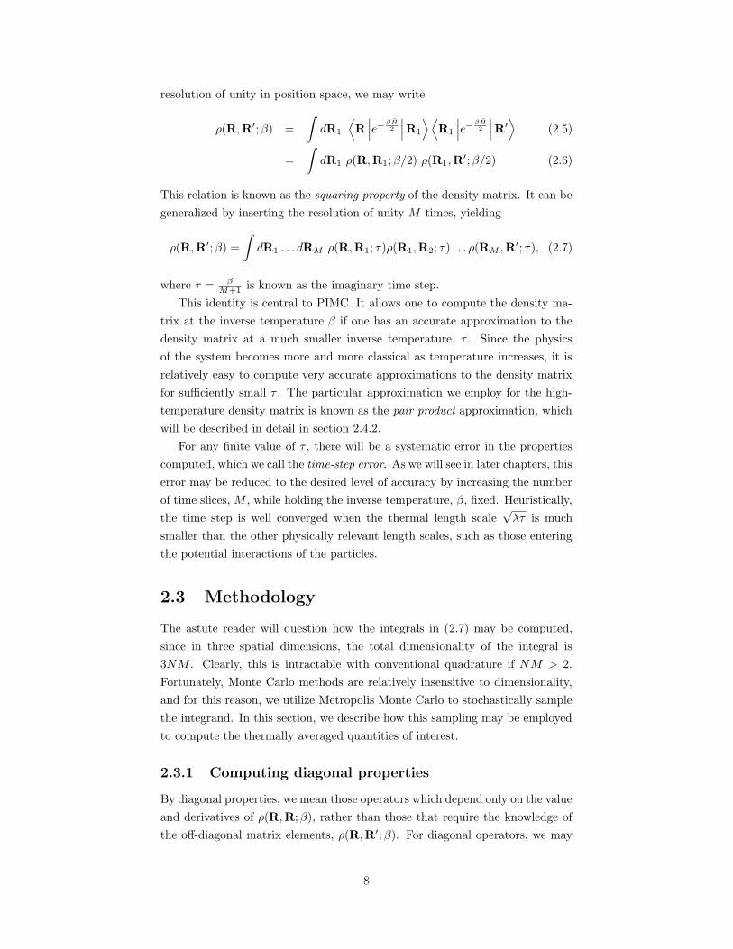
This relation is known as the squaring property of the density matrix. It can be

generalized by inserting the resolution of unity M times, yielding

ρ(R,R′;β) =

∫

dR1 . . . dRM ρ(R,R1; τ)ρ(R1,R2; τ) . . . ρ(RM ,R′; τ), (2.7)

where τ = βM+1 is known as the imaginary time step.

This identity is central to PIMC. It allows one to compute the density ma-

trix at the inverse temperature β if one has an accurate approximation to the

density matrix at a much smaller inverse temperature, τ . Since the physics

of the system becomes more and more classical as temperature increases, it is

relatively easy to compute very accurate approximations to the density matrix

for sufficiently small τ . The particular approximation we employ for the high-

temperature density matrix is known as the pair product approximation, which

will be described in detail in section 2.4.2.

For any finite value of τ , there will be a systematic error in the properties

computed, which we call the time-step error. As we will see in later chapters, this

error may be reduced to the desired level of accuracy by increasing the number

of time slices, M , while holding the inverse temperature, β, fixed. Heuristically,

the time step is well converged when the thermal length scale√λτ is much

smaller than the other physically relevant length scales, such as those entering

the potential interactions of the particles.

2.3 Methodology

The astute reader will question how the integrals in (2.7) may be computed,

since in three spatial dimensions, the total dimensionality of the integral is

3NM . Clearly, this is intractable with conventional quadrature if NM > 2.

Fortunately, Monte Carlo methods are relatively insensitive to dimensionality,

and for this reason, we utilize Metropolis Monte Carlo to stochastically sample

the integrand. In this section, we describe how this sampling may be employed

to compute the thermally averaged quantities of interest.

2.3.1 Computing diagonal properties

By diagonal properties, we mean those operators which depend only on the value

and derivatives of ρ(R,R;β), rather than those that require the knowledge of

the off-diagonal matrix elements, ρ(R,R′;β). For diagonal operators, we may

8

then write⟨

Odiag

⟩

=1

Z

∫

dR0 Oρ(R0,R0;β) (2.8)

We now expand ρ as above, yielding

⟨

Odiag

⟩

=1

Z

∫

dR0 . . . dRM Oρ(R0,R1; τ)ρ(R1,R2; τ) . . . ρ(RM ,R; τ).

(2.9)

Now, define

O(Ri,Ri+1; τ) ≡Oρ(Ri,Ri+1; τ)

ρ(Ri,Ri+1; τ). (2.10)

Then,

⟨

Odiag

⟩

=1

Z

∫

dR0 . . . dRM O(R0,R1; τ)

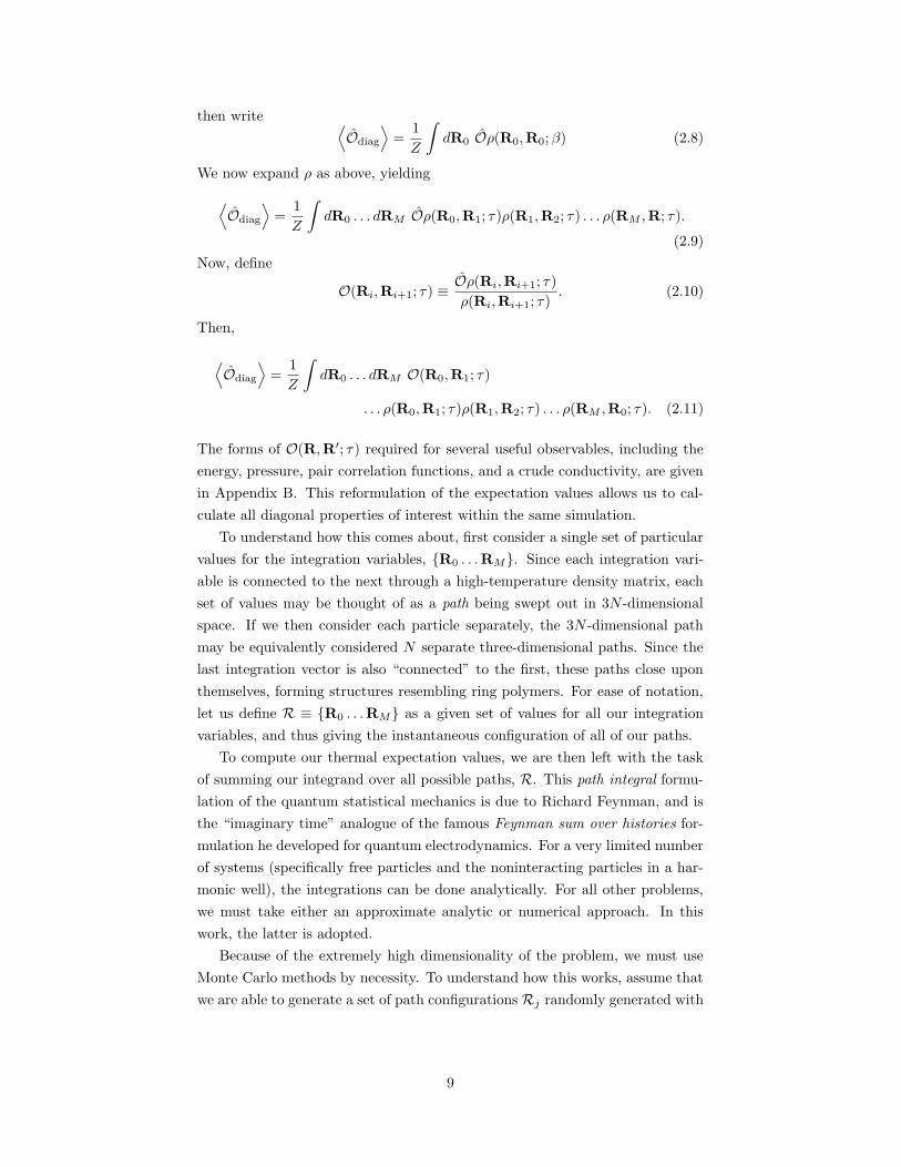
. . . ρ(R0,R1; τ)ρ(R1,R2; τ) . . . ρ(RM ,R0; τ). (2.11)

The forms of O(R,R′; τ) required for several useful observables, including the

energy, pressure, pair correlation functions, and a crude conductivity, are given

in Appendix B. This reformulation of the expectation values allows us to cal-

culate all diagonal properties of interest within the same simulation.

To understand how this comes about, first consider a single set of particular

values for the integration variables, R0 . . .RM. Since each integration vari-

able is connected to the next through a high-temperature density matrix, each

set of values may be thought of as a path being swept out in 3N -dimensional

space. If we then consider each particle separately, the 3N -dimensional path

may be equivalently considered N separate three-dimensional paths. Since the

last integration vector is also “connected” to the first, these paths close upon

themselves, forming structures resembling ring polymers. For ease of notation,

let us define R ≡ R0 . . .RM as a given set of values for all our integration

variables, and thus giving the instantaneous configuration of all of our paths.

To compute our thermal expectation values, we are then left with the task

of summing our integrand over all possible paths, R. This path integral formu-

lation of the quantum statistical mechanics is due to Richard Feynman, and is

the “imaginary time” analogue of the famous Feynman sum over histories for-

mulation he developed for quantum electrodynamics. For a very limited number

of systems (specifically free particles and the noninteracting particles in a har-

monic well), the integrations can be done analytically. For all other problems,

we must take either an approximate analytic or numerical approach. In this

work, the latter is adopted.

Because of the extremely high dimensionality of the problem, we must use

Monte Carlo methods by necessity. To understand how this works, assume that

we are able to generate a set of path configurations Rj randomly generated with

9

a probability density given by

π(Rj) =1

Zρ(R0,R1; τ) . . . ρ(RM ,R0; τ) (2.12)

If we have N such configurations, we may then estimate the thermal expectation

value for operator O by

⟨

O⟩

≈ 1

N

N∑

j=1

O(Rji ,R

ji+1; τ), (2.13)

where the j now indexes the entire path configuration, Rj .

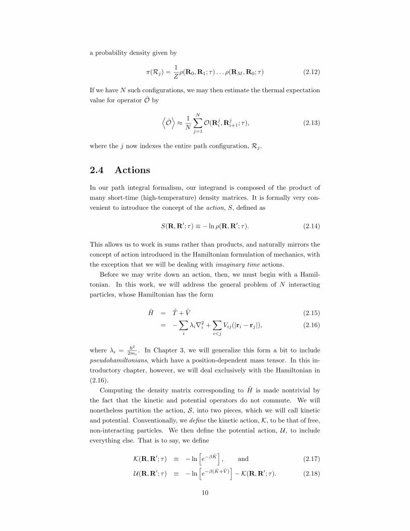
2.4 Actions

In our path integral formalism, our integrand is composed of the product of

many short-time (high-temperature) density matrices. It is formally very con-

venient to introduce the concept of the action, S, defined as

S(R,R′; τ) ≡ − ln ρ(R,R′; τ). (2.14)

This allows us to work in sums rather than products, and naturally mirrors the

concept of action introduced in the Hamiltonian formulation of mechanics, with

the exception that we will be dealing with imaginary time actions.

Before we may write down an action, then, we must begin with a Hamil-

tonian. In this work, we will address the general problem of N interacting

particles, whose Hamiltonian has the form

H = T + V (2.15)

= −∑

i

λi∇2i +

∑

i<j

Vij(|ri − rj |), (2.16)

where λi = ~2

2mi. In Chapter 3, we will generalize this form a bit to include

pseudohamiltonians, which have a position-dependent mass tensor. In this in-

troductory chapter, however, we will deal exclusively with the Hamiltonian in

(2.16).

Computing the density matrix corresponding to H is made nontrivial by

the fact that the kinetic and potential operators do not commute. We will

nonetheless partition the action, S, into two pieces, which we will call kinetic

and potential. Conventionally, we define the kinetic action, K, to be that of free,

non-interacting particles. We then define the potential action, U , to include

everything else. That is to say, we define

K(R,R′; τ) ≡ − ln[

e−βK]

, and (2.17)

U(R,R′; τ) ≡ − ln[

e−β(K+V )]

−K(R,R′; τ). (2.18)

10

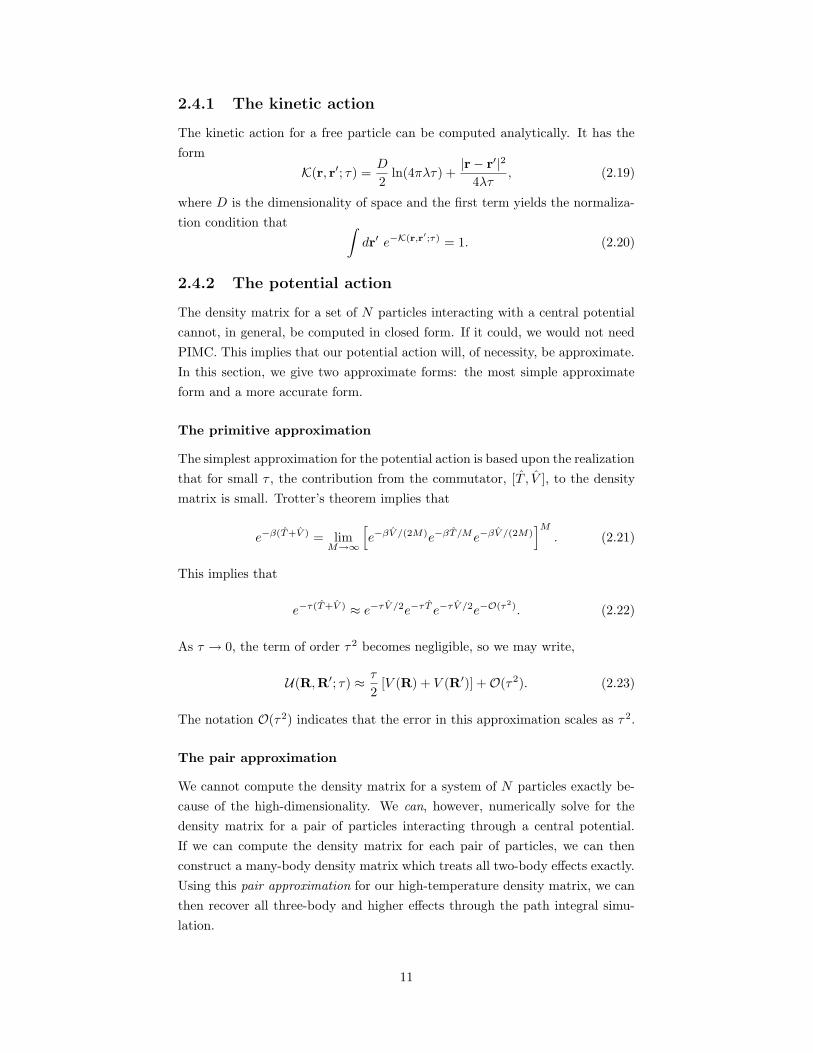
2.4.1 The kinetic action

The kinetic action for a free particle can be computed analytically. It has the

form

K(r, r′; τ) =D

2ln(4πλτ) +

|r− r′|24λτ

, (2.19)

where D is the dimensionality of space and the first term yields the normaliza-

tion condition that ∫

dr′ e−K(r,r′;τ) = 1. (2.20)

2.4.2 The potential action

The density matrix for a set of N particles interacting with a central potential

cannot, in general, be computed in closed form. If it could, we would not need

PIMC. This implies that our potential action will, of necessity, be approximate.

In this section, we give two approximate forms: the most simple approximate

form and a more accurate form.

The primitive approximation

The simplest approximation for the potential action is based upon the realization

that for small τ , the contribution from the commutator, [T , V ], to the density

matrix is small. Trotter’s theorem implies that

e−β(T+V ) = limM→∞

[

e−βV /(2M)e−βT/Me−βV /(2M)]M

. (2.21)

This implies that

e−τ(T+V ) ≈ e−τV /2e−τT e−τV /2e−O(τ2). (2.22)

As τ → 0, the term of order τ 2 becomes negligible, so we may write,

U(R,R′; τ) ≈ τ

2[V (R) + V (R′)] +O(τ2). (2.23)

The notation O(τ 2) indicates that the error in this approximation scales as τ 2.

The pair approximation

We cannot compute the density matrix for a system of N particles exactly be-

cause of the high-dimensionality. We can, however, numerically solve for the

density matrix for a pair of particles interacting through a central potential.

If we can compute the density matrix for each pair of particles, we can then

construct a many-body density matrix which treats all two-body effects exactly.

Using this pair approximation for our high-temperature density matrix, we can

then recover all three-body and higher effects through the path integral simu-

lation.

11

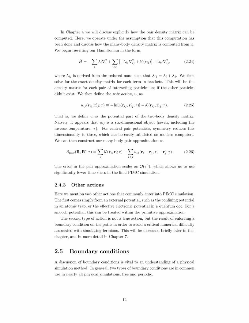
In Chapter 4 we will discuss explicitly how the pair density matrix can be

computed. Here, we operate under the assumption that this computation has

been done and discuss how the many-body density matrix is computed from it.

We begin rewriting our Hamiltonian in the form,

H = −∑

i

λi∇2i +

∑

i<j

[−λij∇2

ij + V (rij)]+ λij∇2

ij , (2.24)

where λij is derived from the reduced mass such that λij = λi + λj . We then

solve for the exact density matrix for each term in brackets. This will be the

density matrix for each pair of interacting particles, as if the other particles

didn’t exist. We then define the pair action, u, as

uij(rij , r′ij ; τ) ≡ − ln[ρ(rij , r

′ij ; τ)]−K(rij , r

′ij ; τ). (2.25)

That is, we define u as the potential part of the two-body density matrix.

Naively, it appears that uij is a six-dimensional object (seven, including the

inverse temperature, τ). For central pair potentials, symmetry reduces this

dimensionality to three, which can be easily tabulated on modern computers.

We can then construct our many-body pair approximation as

Spair(R,R′; τ) =

∑

i

K(ri, r′i; τ) +

∑

i<j

uij(ri − rj , r′i − r′j ; τ) (2.26)

The error in the pair approximation scales as O(τ 3), which allows us to use

significantly fewer time slices in the final PIMC simulation.

2.4.3 Other actions

Here we mention two other actions that commonly enter into PIMC simulation.

The first comes simply from an external potential, such as the confining potential

in an atomic trap, or the effective electronic potential in a quantum dot. For a

smooth potential, this can be treated within the primitive approximation.

The second type of action is not a true action, but the result of enforcing a

boundary condition on the paths in order to avoid a critical numerical difficulty

associated with simulating fermions. This will be discussed briefly later in this

chapter, and in more detail in Chapter 7.

2.5 Boundary conditions

A discussion of boundary conditions is vital to an understanding of a physical

simulation method. In general, two types of boundary conditions are in common

use in nearly all physical simulations, free and periodic.

12

2.5.1 Free

In free boundary conditions, the particles move throughout infinite space, re-

stricted only by their potential interactions with each other. While this can be

very useful for simulating isolated systems, care must be taken. For example we

can imagine simulating a molecule under such conditions. Since the Coulomb

interactions decay as 1/r, however, one must remember that thermal ionization

can take place at any nonzero temperature. That is, an electron can wander

off the molecule into free space, never to return. While this is a physical effect,

and not an artifact of the simulation, it is usually not a useful one to simulate.

Therefore, care must be taken to detect this condition and correct it if one

wishes to compute properties of the neutral molecule. The effect is all the more

pronounced with potentials which decay faster than 1/r, such as the interaction

of two helium atoms.

2.5.2 Periodic

Periodic boundary conditions are a staple of the condensed matter community.

In this scheme, we establish a simulations cell (usually a rectangular box) and

the condition that all coordinates are considered to be taken modulo the box

lengths. That is to say that a particle leaving the top of the simulation cell

immediately reenters from the bottom, etc.

These conditions are particularly useful when one is attempting to calculate

bulk properties, since surface effects are largely eliminated. In free boundary

conditions, one must simulate an enormous number (> 106) of atoms to ap-

proach the bulk limit. The same limit can be approached much more rapidly in

periodic boundary conditions, since in the simulation, there are no identifiable

surfaces. Finite size effects remain, however, because there exists unnatural

correlations between the particles in the simulation cell and those in adjacent

cells.

Working in periodic boundary conditions may introduce additional technical

challenges if any of our interaction potentials are long-range, i.e. they fall off

with distance, r, no faster than r−2. The Coulomb potential, nearly ubiquitous

in atomic-level simulation, is the prototypical example. When working in peri-

odic boundary conditions, one must sum the interactions of each particle with

the others in the simulation cell, but also over all the periodic images of the

particles. Unfortunately, for long-range potentials this summation, if performed

naively, does not converge. Special methods have been developed to perform

the summation such that it converges rapidly for systems with no net charge.

These methods will be described in detail in Chapter 5.

13

2.5.3 Mixed

It is also possible to mix periodic and and free boundary conditions in the same

simulation. For example, imagine one is interested in studying the properties of

the surface of a solid material. It may be appropriate to have periodic bound-

ary conditions in the dimensions coplanar with the surface, while allowing free

boundary conditions in the direction normal to the surface. These slab boundary

conditions will not be discussed further in this work.

2.6 Quantum statistics: bosons and fermions

Thus far, our discussion of the path integral method has assumed that particles

are distinguishable (i.e. boltzmannons). We know, of course, that all funda-

mental particles obey either Fermi or Bose statistics. If P is an operator which

permutes the position vector R, then the boson density matrix, ρB , may be

written in terms of the distinguishable particle density matrix, ρD as

ρB(R,R′;β) =1

N !

∑

PρD(PR,R′;β). (2.27)

For fermions, an additional sign enters the sum, reflecting the antisymmetry,

ρB(R,R′;β) =1

N !

∑

P(−1)PρD(PR,R′;β), (2.28)

where the (−1)P reflects the sign of the permutation: negative for an odd

number of pair permutations and positive for an even number.

In principle, the summation could be done explicitly for the short-time den-

sity matrix. However, such evaluation would be extremely costly. Instead, we

use Monte Carlo to sample the permutation sum as the entire simulation pro-

gresses. The permutation then becomes a part of the Monte Carlo state. For

bosons, this is a relatively straightforward matter since all the terms are posi-

tive. The negative contributions to the fermions sum are problematic, however,

since they cannot be treated as a probability. This problem will be addressed

in Chapter 7.

In terms of the PIMC simulation, the permutation can be thought of as a

topological property of the paths – it determines how the paths are connected.

Consider a system of N identical particles with M time slices. In the simplest

case, the identity permutation, each particle path closes upon itself, i.e. time

slice 0 of each particle is connected to time sliceM . If we add a pair permutation

between particles 1 and 2, those particle paths close upon each other forming

a single closed ring polymer of 2M links. In principle permutations of any

length can occur in bosonic systems at low temperature. The presence of large

permutation cycles is tightly connected with Bose condensation and superfluid

behavior. Details of sampling permutations within PIMC will be discussed in

14

section 2.8.6.

2.7 Classical particles

In general, the kinetic action restricts the spatial extent of a particle path to

the order of Λ ≡√

~2β/2m. For very heavy particles at relatively high temper-

atures, this length scale is much smaller than any of the other relevant length

scales of the system. This is often the case in the combined simulation of elec-

trons and nuclei. For example, in the simulation of sodium ions and electrons,

Λe ≈ 200ΛNa. In this case, it is quite a reasonable approximation to set ΛNa = 0.

That is to say that we will simulate the sodium ions as classical particles. In

terms of the PIMC simulation, this is equivalent to the requirement that each

sodium ion be at the same position at every time slice.

2.8 Moving the paths

2.8.1 Metropolis Monte Carlo

The path integral Monte Carlo algorithms described in this thesis are sophisti-

cated examples of Metropolis Monte Carlo. In this algorithm, the Monte Carlo

state of the system is sampled through a process of proposing a random change

of state, followed by accepting or rejecting that change with a given probability.

In particular, let us consider the probability distribution given by

P (s) =π(s)

∑

s′ π(s′). (2.29)

The Monte Carlo state, s, may be as simple as a single integer, or as complex

as high-dimensional vector in continuous space. We begin at state s. We then

propose a move to a new state, s′, chosen randomly, e.g. a displacement from

the present position. We must know a priori the probability, T (s → s′), of

constructing the new state, s′, given the present state, s. Furthermore, we must

know the probability for the reverse process, T (s′ → s). Once these quantities

are known, we compute the acceptance probability as

A(s→ s′) = min

[

1,π(s′)T (s′ → s)

π(s)T (s→ s′)

]

. (2.30)

This choice of the acceptance ratio satisfies a condition known as detailed bal-

ance. This condition states that once equilibrium is reached, the total rate of

transitions from state s to s′ is the same as the rate of transitions from s′ to s.

Algebraically,

π(s)T (s→ s′)A(s→ s′) = π(s′)T (s′ → s)A(s′ → s). (2.31)

15

We add the additional requirement that any state s∗ can be reached from any

other state, s, in a finite number of Monte Carlo moves. An algorithm that

satisfies this is called ergodic. Detailed balance and ergodicity together guaran-

tee that an algorithm will sample the equilibrium distribution in the long-time

limit.

These are sufficient, but not necessary, conditions for sampling π(s). In

particular, there exist algorithms which do not obey detailed balance, but still

sample π(s) in the long-time limit. Such algorithms, however, must be consid-

ered individually, while Metropolis Monte Carlo provides a nearly automatic

prescription for constructing a correct algorithm.

In PIMC, the Monte Carlo state, s, is given by the positions of each particle

at each time slice, for which we have used the notation R. The corresponding

probability density, π(R), is then given in terms of the action, S, as

π(R) = e−S(R). (2.32)

2.8.2 Multistage Metropolis Monte Carlo

The basic Metropolis algorithm can be generalized to include multiple stages in

a given move. In each stage, an update of some subset of the path variables,

Rn, is proposed. This proposal is then accepted or rejected on the basis of the

ratio of transition probabilities, as before, and on the change in the stage action,

which we will discuss momentarily. If the stage is accepted, the algorithm passes

to the next stage. If it is rejected, all stages of the move are rejected and we

proceed to the next move. If the final stage is accepted, all stages are accepted

and we again proceed.

Each stage has a stage action associated with it. We write the action for the

nth stage as Sn(Rn). We can then write the acceptance probability as

A(Rn → R′n) = min

[

1,exp [−Sn(R′

n) + Sn−1(Rn−1)] T (R′n → Rn)

exp[−Sn(Rn) + Sn−1(R′

n−1)]T (Rn → R′

n)

]

(2.33)

For all stages but the last, the stage action need not be exact. The final

stage action, however, must reflect the desired sampling distribution. It should

be noted, however, that a poorly chosen stage action can cause problems with

ergodicity. In particular, if the acceptance probability at an early stage is zero

when the true probability is nonzero, the algorithm will not be ergodic. This is

known as undersampling.

The main motivation for the introduction of the multistage scheme is for

the sake of improved computational efficiency. In many cases, if reasonably

accurate stage actions exist, we can detect early a move which is very unlikely

to be accepted and bail out without completing the rest of the move. This can

save a significant percentage of the total run time.

16

level 0

level 1

level 2

level 3

level 4

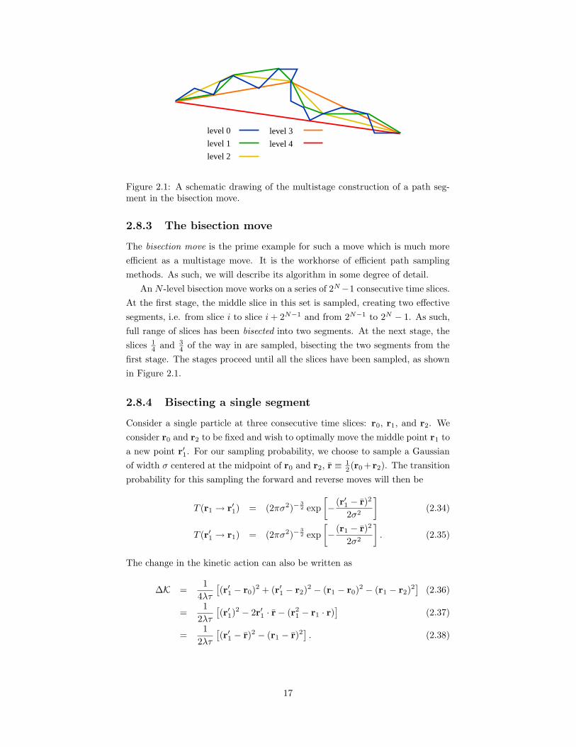
Figure 2.1: A schematic drawing of the multistage construction of a path seg-ment in the bisection move.

2.8.3 The bisection move

The bisection move is the prime example for such a move which is much more

efficient as a multistage move. It is the workhorse of efficient path sampling

methods. As such, we will describe its algorithm in some degree of detail.

An N -level bisection move works on a series of 2N−1 consecutive time slices.

At the first stage, the middle slice in this set is sampled, creating two effective

segments, i.e. from slice i to slice i+ 2N−1 and from 2N−1 to 2N − 1. As such,

full range of slices has been bisected into two segments. At the next stage, the

slices 14 and 3

4 of the way in are sampled, bisecting the two segments from the

first stage. The stages proceed until all the slices have been sampled, as shown

in Figure 2.1.

2.8.4 Bisecting a single segment

Consider a single particle at three consecutive time slices: r0, r1, and r2. We

consider r0 and r2 to be fixed and wish to optimally move the middle point r1 to

a new point r′1. For our sampling probability, we choose to sample a Gaussian

of width σ centered at the midpoint of r0 and r2, r ≡ 12 (r0 +r2). The transition

probability for this sampling the forward and reverse moves will then be

T (r1 → r′1) = (2πσ2)−32 exp

[

− (r′1 − r)2

2σ2

]

(2.34)

T (r′1 → r1) = (2πσ2)−32 exp

[

− (r1 − r)2

2σ2

]

. (2.35)

The change in the kinetic action can also be written as

∆K =1

4λτ

[(r′1 − r0)

2 + (r′1 − r2)2 − (r1 − r0)

2 − (r1 − r2)2]

(2.36)

=1

2λτ

[(r′1)

2 − 2r′1 · r− (r21 − r1 · r)

](2.37)

=1

2λτ

[(r′1 − r)2 − (r1 − r)2

]. (2.38)

17

The the acceptance probability for this is given by

A =T (r′1 → r1)

T (r1 → r′1)exp(−∆K) exp(−∆V ) (2.39)

=exp

[

− (r1−r)2

2σ2

]

exp[

− (r′1−r)2

2σ2

]

exp[

− (r′1−r)2

2λτ

]

exp[

− (r1−r)2

2λτ

] exp(−∆V ). (2.40)

We see that by making the choice of σ2 = λτ , that the acceptance probability

becomes equal to one for free particles. This means that this construction ex-

actly samples the kinetic action. This prescription is easily modified to sampling

segments at higher bisection levels by making the choice

σ2 = 2`λτ, (2.41)

where ` is the bisection level, with ` = 0 corresponding to the last stage of the

move.

2.8.5 The displace move

While the bisection move is very efficient at sampling the details of a range of

time slices, the acceptance ratio decreases rapidly with the number of bisection

levels. As a result, it is often the case that only a fraction of the total number

of time slices may be sampled by a bisection move. This, in turn, results in a

very slow diffusion of the centroid of the path. Thus, a useful complement to

the bisection move is one which simply rigidly translates the entire path by a

random displacement vector. This move, termed here the displace move, may

be applied to the electron paths or to the classical ions.

The actual displacement vector may be chosen is several ways. Commonly,

a vector generated from a Gaussian distribution is chosen. This choice is par-

ticularly simple, since the ratio of the reverse to forward transition probabilities

is unity. The width, σ of the distribution may then be selected to optimize

efficiency. A rule of thumb is to choose σ so that about twenty percent of the

moves are accepted, but this may not produce the optimum efficiency.

In the case of the application of this move to ions, an enhancement may

added to improve efficiency. In an algorithm known as Smart Monte Carlo

[2], ions are displaced not only by a randomly chosen vector, by also by a

deterministic amount in the direction of the forces on the ions. In this case,

the ratio of the transition probabilities for the reverse and forward moves is no

longer unity. It usually results, however, in an increase in the acceptance ratio

and a decrease in the autocorrelation time for the system.

18

PSfrag replacements

01 2

β

x

2`τ

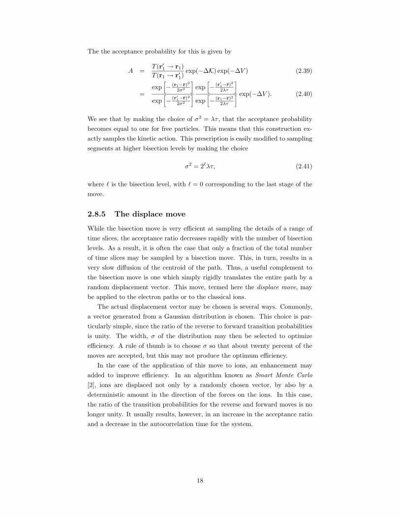
Figure 2.2: Schematic of creating a pair permutation in one dimension. Thehorizontal axis is position and the vertical axis imaginary time. In the move, aregion of size 2`τ of the paths of two particles is erased (red) and reconstructed(green) with swapped end points. The entire change is accepted or rejectedbased on the change in action and ratio of the sampling probabilities.

2.8.6 Sampling permutation space

Before we begin describing the algorithms used for sampling permutation space,

we must discuss how the permutation is represented in the Monte Carlo state

space. The simplest and most efficient representation is to simply store a vector

of integers equal in size to the number of particles. The value stored at index i,

Pi, represents the particle onto which particle i permutes. This may be i itself

(an unpermuted particle) or another particle. The permutation may be applied

at any time slice. Therefore, as meta-data, we store the time slice after which

the permutation acts. We refer to this slice as the join slice.

To sample permutation space, we propose a move which changes the per-

mutation vector. We then use the bisection move to construct new paths for

the permuted particles. The entire permutation/bisection move is accepted or

rejected as a whole based on the change in action. This is shown schematically

in Figure 2.2.

As the figure shows, a range of time slices of size 2` is first chosen. A cyclic

permutation containing typically two to four particles is then proposed. The

section of those particles in the selected range of time slices is then erased.

For each particle, i, in the proposed permutation cycle, a new path segment

which terminates in Pi is constructed with the bisection method. Finally, the

combined permutation/bisection move is accepted or rejected as a whole with

the computed acceptance probability.

19

All that is left to describe is a method to propose permutations. For a very

small system containing only a few (e.g. five) identical particles, the permutation

vector may be generated randomly from all valid permutations. Unfortunately,

this simple method becomes extremely inefficient as the system size grows since

almost all proposed moves will be rejected.

It is necessary, then, to have an algorithm which proposes permutations

which are likely to be accepted. Here we describe one such algorithm. Let us

imagine we wish to attempt a permutation cycle over the range of time slices

from i to i + 2`. The dominant cause for rejecting a randomly selected per-

mutation is the increase in kinetic action it requires. For a pair permutation,

for example, permuting particle paths must be sufficiently close or the recon-

structed paths will necessarily have a very high kinetic action, which will result

in the move’s rejection. We therefore wish to select moves based on the expected

change in kinetic action, which may be done as follows.

Consider first a pair permutation between particles a and b. Let the position

of particle a at time slices i and i+2` be written ra and r′a, respectively, and like-

wise for particle b. The expected change in kinetic action for this permutation

may then be given by

∆K =1

2`+2λτ

[(r′b − ra)2 + (rb − r′a)2 − (r′b − rb)

2 − (r′a − ra)2]. (2.42)

We then sample the permutation with the transition probability

T [R → Pab(R)] = Nexp

[−(r′b−ra)2

2`+1λτ

]

exp[−(r′a−ra)2

2`+1λτ

]

exp[−(r′a−rb)

2

2`+1λτ

]

exp[−(r′

b−rb)2

2`+1λτ

] , (2.43)

where N is the normalization constant. Furthermore, we note that

T [Pab(R)→ R] = T [R → Pab(R)]−1. (2.44)

With this choice, the ratio of the forward and reverse transition probabilities

will cancel the expected change in kinetic action. For free particles, then, we

will achieve 100% acceptance.

For convenience, we define

tab ≡exp

[−(r′b−ra)2

2`+1λτ

]

exp[−(r′a−ra)2

2`+1λτ

] . (2.45)

Our transition probability for the two-particle permutation can then be written

as T [R → Pab(R)] = Ntabtba. Written this way, we see that we can generalize

to a three-particle permutation by writing, T [R → Pabc(R)] = Ntabtbctca. We

can similarly generalize to an N -particle cycle. We can then construct a table of

possible permutations to propose and their respective probabilities. For compu-

20

tation tractability, we generally truncate the table at four-particle cycles. The

normalization can then be written as

N =∑

a

[

taa +∑

b

tab

[

tba +∑

c

tbc

[

tca +∑

d

tcdtda

]]]

, (2.46)

where taa = 1. Thus a system of N particles will require a table of size O(N 4).

For large systems, this can be reduced greatly by discarding elements with

probability below some cutoff, ε. This results in some approximation, but a

very well controlled one if ε chosen sufficiently small.

Once the table is constructed, permutations may be drawn randomly by

generating a random number, ξ, uniformly distributed between 0 and 1. Label

the ith entry in the table of possible permutations pi. We can then define the

cumulative probability, cj as

cj =∑

i≤j

pi. (2.47)

We then perform a bisection search through the table and locate the entry

such that cj−1 < ξ ≤ cj . We will then have selected pj with the appropriate

probability. Once the permutation is selected, we must construct a new table

for the reverse move in order to compute the appropriate transition probability

ratio. We then proceed to the bisection stages, as described above, and accept

or reject the move as a whole.

2.9 Putting it together: the PIMC algorithm

Once we have constructed our actions, moves, and observables, the overall al-

gorithm is straight forward. We simply alternate between making Monte Carlo

moves to update the paths and computing observable estimators on the present

path. We must only choose the number of MC steps to make between com-

puting observables. This is usually chosen so that each observation is relatively

independent of the last. This is to prevent wasting CPU time by computing

highly-correlated samples. If some residual autocorrelation remains, this is de-

termined a posteriori during the statistical analysis of the run.

Periodically, after a block of N observations have been made, the average

for that block is written to disk for each observable. The choice of N is not

critical. It should only be chosen large enough that excessive disk storage is not

required for the run, and small enough that there are at least some tens of blocks

with which we may compute error bars with confidence. Writing periodically

to disk also allows us to salvage data from run which are terminated early due

to machine failure. After the run is completed, we perform the rudimentary

statistical analysis on the data to determine mean values and error bars for our

observables.

21

References

[1] D.M. Ceperley. Path integrals in the theory of condensed helium. Rev. Mod.

Phys., 67(2):279, April 1995.

[2] P.J. Rossky, J.D. Doll, and H.L. Friedman. Brownian dynamics as smart

Monte Carlo simulation. J. Chem. Phys., 26:4628–4633, 1978.

22

Chapter 3

Pseudohamiltonians

3.1 Difficulties associated with heavy atoms

Path integral Monte Carlo has proven to be very accurate and effective for sim-

ulations of hydrogen at the level of proton and electrons. It would then be

desirable to apply the method to systems containing heavier atoms. Unfortu-

nately, in naive implementations, such simulations rapidly become prohibitively

expensive from a computational point of view. To see why, let us estimate the

cost of simulating N atoms with atomic number Z to a fixed statistical error in

the energy, ∆E. For a charge-neutral system, we will then have NZ electrons.

Since electrons are fermions, current quantum Monte Carlo methods require the

evaluation of the Slater determinant. Known algorithms for evaluating deter-

minants scale as (NZ)3.

Now consider the innermost core state of the atom with atomic number Z.

The most tightly-bound s-state will have a wave function with the asymptotic

behavior, u(r) = e−Zr. This gives a characteristic feature size proportional to

Z−1. The characteristic length in a path integral simulation is τ12 . Therefore,

with a fixed inverse temperature, β, the number of time slices, M , is proportional

to Z2. Finally, we must consider the variation of the total energy per atom.

The mostly tightly bound core state has an energy proportional to Z2. Taken

together, these considerations imply that the CPU time required to obtain a

fixed energy accuracy per atom scales as approximately Z6.

3.2 Pseudopotentials

It has long been recognized by chemists and physicists that the bonding proper-

ties of atoms is determined almost entirely by the valence states of the involved

atoms. In most physical circumstances of interest, the high binding energy of

the core states make them essentially an inert system off which the valence

electrons scatter. This motivates the pseudopotential (PP) approximation, in

which the combined system of the nucleus and core states is replaced by an ef-

fective potential which is designed to have scattering properties which are nearly

identical to that of the ion core. If a pseudopotential is able to reproduce the

appropriate scattering properties over a wide range of chemical environments,

23

it is said to be transferable. An excellent review of the use of pseudopotentials

for condensed matter physics is given by Pickett [9].

3.2.1 Local pseudopotentials

The simplest form of pseudopotentials are local. In this case the potential op-

erator takes the simple form of a function of the radial distance, V (r). Because

of their simplicity, local pseudopotentials (LPPs) are very efficient and easy

to implement in codes. For some elements, notably simple metals and some

semiconductors, local pseudopotentials give quite accurate results. For other

elements, however, it is not possible to construct an accurate and transferable

local pseudopotential. For these cases a more sophisticated approach is needed.

3.2.2 Nonlocal pseudopotentials

The main factor limiting the accuracy of LPPs is the fact that an electron

in an s-state scatters differently than one in a p or d state. This reflects the

fact that the constraints imposed by Pauli exclusion introduce different effective

potentials for states of different symmetry. Hence, for many elements, a different

scattering potential is required for each angular momentum channel in order to

attain transferability. In order to achieve this, the potential operator may be

constructed from nonlocal projections. In particular, for an atom centered at

the origin, we may write

VNL =∑

l

∑

−l≤m≤l

|lm〉 〈lm|Vl(r), (3.1)

Where the |lm〉〈lm| project out each spherical harmonic.

Nonlocal pseudopotentials (NLPPs) have much more flexibility in matching

the scattering properties of a given atom core. As a result, they are much more

transferable than LPPs. However, this higher accuracy comes at the cost of

additional code complexity and computational cost. In DFT calculations which

work in a plane wave basis, for example, applying NLPPs to the electrons takes

a significant fraction of the total computation time.

Problems with QMC and solutions

NLPPs were developed within the context of the single-particle methods de-

scribed in section 1.2.2. These methods work in a basis and, as such, it is not

difficult to apply the nonlocal projection operators. Continuum QMC methods,

however, sample electron positions directly. This distinction causes additional

difficulties in using NLPPs in these methods.

In particular, consider diffusion Monte Carlo (DMC). In this method, the

ground state is projected out of a trial wave function ψT by repeated application

of the Green’s function, exp(−τH). Since the exponentiation of the projection

24

operators cannot be easily done in Monte Carlo, an approximation is used in

which the projection operators are applied to ψT in order to localize the Hamil-

tonian [6]. This localization approximation implicitly makes the Hamiltonian

dependent on the trial wave function and destroys the variational principle of

diffusion Monte Carlo. Fortunately, if an accurate trial wave function is used,

the localization approximation is not severe and in most cases introduces a

smaller error than the pseudopotential approximation itself.

Problems with PIMC

Unfortunately, the localization approximation used in diffusion Monte Carlo

cannot easily be transfered to PIMC. A number of issues exist. First, contrary to

the case in DMC, accurate finite temperature trial density matrices are usually

unavailable in PIMC. For simulations including electrons, we do include a trial

density matrix to enforce a node or phase constraint, which will be discussed

in Chapter 7. In general, however, the results generated by these restricted

PIMC methods do not depend very strongly on the quality of the trial function

employed. The introduction of an implicit dependence on the Hamiltonian is

thus undesirable for this reason.

A second, perhaps more fundamental problem exists. If we apply the non-

local operator to a finite-temperature many-body density matrix, the result is

still nonlocal. This may be seen by writing the density matrix in a sum-over-

eigenstates expansion.

ρT (R,R′;β) =1

Z

∑

i∈eig. states

e−βEiψ∗i (R)ψi(R

′). (3.2)

Applying VNL

VNLρT (R,R′;β)

ρT (R,R′;β)=

∑

i e−βEi

(

VNLψ∗i (R)

)

ψi(R′)

∑

i e−βEiψ∗

i (R)ψi(R′). (3.3)

Unfortunately, this sum does not reduce to a simple function of R, except in

the limit of β →∞. In this latter case, only the ground state contributes to the

sum, and we have the same result as in DMC.

This property is evocative of a possible solution. Rather than apply the

NLPP to a trial density matrix, we may apply it to a trial wave function with

an additional approximation. It is reasonable to expect that at relatively low

temperatures, the induced systematic error would not be severe, provided an

accurate wave function is available. It does, however, introduce the rather

disagreeable requirement of generating an optimized wave function for each ion

configuration. For these reasons, we seek an alternative formulation which has

greater transferability than local pseudopotentials without the complications

NLPPs introduce.

25

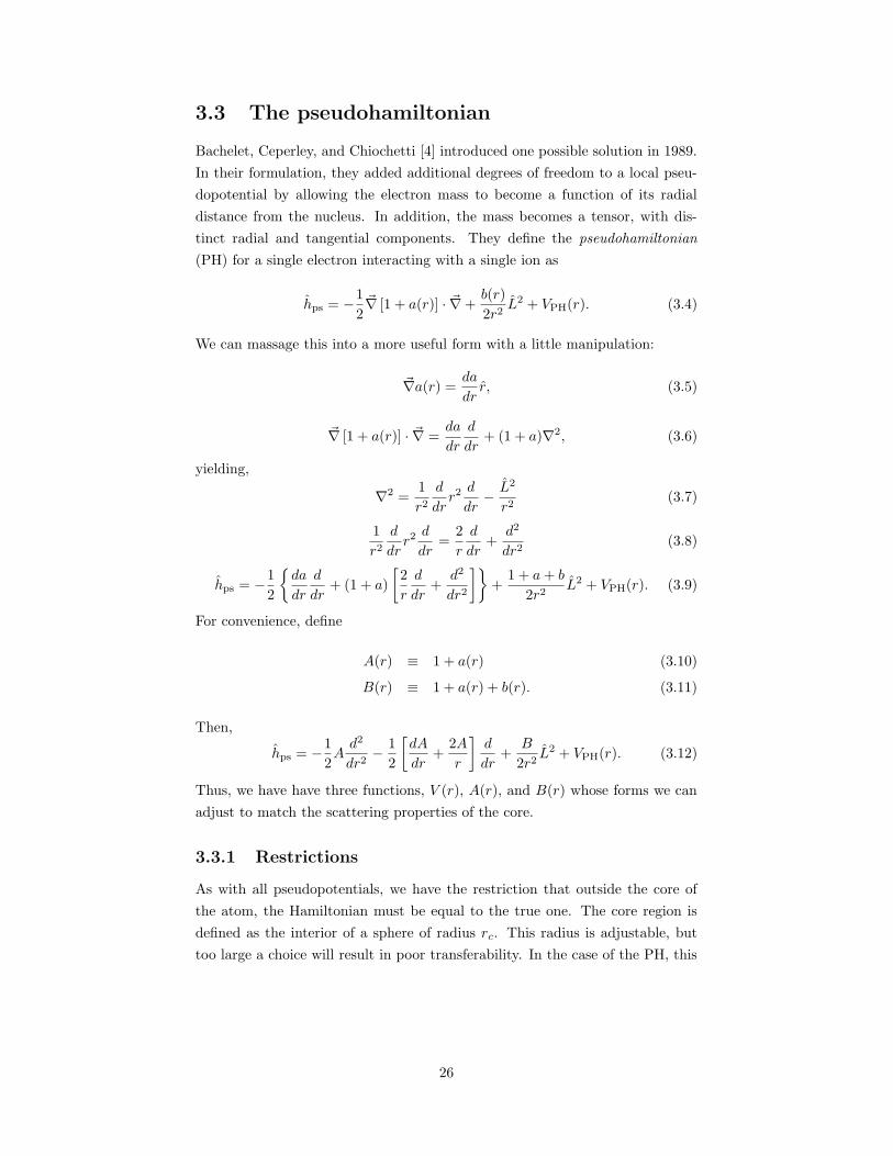
3.3 The pseudohamiltonian

Bachelet, Ceperley, and Chiochetti [4] introduced one possible solution in 1989.

In their formulation, they added additional degrees of freedom to a local pseu-

dopotential by allowing the electron mass to become a function of its radial

distance from the nucleus. In addition, the mass becomes a tensor, with dis-

tinct radial and tangential components. They define the pseudohamiltonian

(PH) for a single electron interacting with a single ion as

hps = −1

2~∇ [1 + a(r)] · ~∇+

b(r)

2r2L2 + VPH(r). (3.4)

We can massage this into a more useful form with a little manipulation:

~∇a(r) =da

drr, (3.5)

~∇ [1 + a(r)] · ~∇ =da

dr

d

dr+ (1 + a)∇2, (3.6)

yielding,

∇2 =1

r2d

drr2d

dr− L2

r2(3.7)

1

r2d

drr2d

dr=

2

r

d

dr+

d2

dr2(3.8)

hps = −1

2

da

dr

d

dr+ (1 + a)

[2

r

d

dr+

d2

dr2

]

+1 + a+ b

2r2L2 + VPH(r). (3.9)

For convenience, define

A(r) ≡ 1 + a(r) (3.10)

B(r) ≡ 1 + a(r) + b(r). (3.11)

Then,

hps = −1

2Ad2

dr2− 1

2

[dA

dr+

2A

r

]d

dr+

B

2r2L2 + VPH(r). (3.12)

Thus, we have have three functions, V (r), A(r), and B(r) whose forms we can

adjust to match the scattering properties of the core.

3.3.1 Restrictions

As with all pseudopotentials, we have the restriction that outside the core of

the atom, the Hamiltonian must be equal to the true one. The core region is

defined as the interior of a sphere of radius rc. This radius is adjustable, but

too large a choice will result in poor transferability. In the case of the PH, this

26

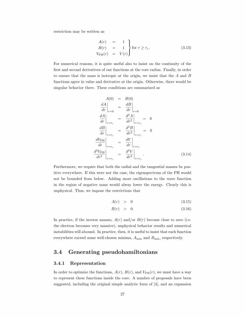
restriction may be written as

A(r) = 1

B(r) = 1

VPH(r) = V (r)

for r ≥ rc. (3.13)

For numerical reasons, it is quite useful also to insist on the continuity of the

first and second derivatives of our functions at the core radius. Finally, in order

to ensure that the mass is isotropic at the origin, we insist that the A and B

functions agree in value and derivative at the origin. Otherwise, there would be

singular behavior there. These conditions are summarized as

A(0) = B(0)

dA

dr

∣∣∣∣r=0

=dB

dr

∣∣∣∣r=0

dA

dr

∣∣∣∣r=rc

=d2A

dr2

∣∣∣∣r=rc

= 0

dB

dr

∣∣∣∣r=rc

=d2B

dr2

∣∣∣∣r=rc

= 0

dVPH

dr

∣∣∣∣r=rc

=dV

dr

∣∣∣∣r=rc

d2VPH

dr2

∣∣∣∣r=rc

=d2V

dr2

∣∣∣∣r=rc

. (3.14)

Furthermore, we require that both the radial and the tangential masses be pos-

itive everywhere. If this were not the case, the eigenspectrum of the PH would

not be bounded from below. Adding more oscillations to the wave function

in the region of negative mass would alway lower the energy. Clearly this is

unphysical. Thus, we impose the restrictions that

A(r) > 0 (3.15)

B(r) > 0. (3.16)

In practice, if the inverse masses, A(r) and/or B(r) become close to zero (i.e.

the electron becomes very massive), unphysical behavior results and numerical

instabilities will abound. In practice, then, it is useful to insist that each function

everywhere exceed some well-chosen minima, Amin and Bmin, respectively.

3.4 Generating pseudohamiltonians

3.4.1 Representation

In order to optimize the functions, A(r), B(r), and VPH(r), we must have a way

to represent these functions inside the core. A number of proposals have been

suggested, including the original simple analytic form of [4], and an expansion

27

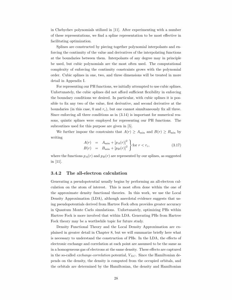
in Chebychev polynomials utilized in [11]. After experimenting with a number

of these representations, we find a spline representation to be most effective in

facilitating optimization.

Splines are constructed by piecing together polynomial interpolants and en-

forcing the continuity of the value and derivatives of the interpolating functions

at the boundaries between them. Interpolants of any degree may in principle

be used, but cubic polynomials are the most often used. The computational

complexity of enforcing the continuity constraints grows with the polynomial

order. Cubic splines in one, two, and three dimensions will be treated in more

detail in Appendix I.

For representing our PH functions, we initially attempted to use cubic splines.

Unfortunately, the cubic splines did not afford sufficient flexibility in enforcing

the boundary conditions we desired. In particular, with cubic splines it is pos-

sible to fix any two of the value, first derivative, and second derivative at the

boundaries (in this case, 0 and rc), but one cannot simultaneously fix all three.

Since enforcing all three conditions as in (3.14) is important for numerical rea-

sons, quintic splines were employed for representing our PH functions. The

subroutines used for this purpose are given in [5].

We further impose the constraints that A(r) ≥ Amin and B(r) ≥ Bmin by

writing

A(r) = Amin + [pA(r)]2

B(r) = Bmin + [pB(r)]2

for r < rc, (3.17)

where the functions pA(r) and pB(r) are represented by our splines, as suggested

in [11].

3.4.2 The all-electron calculation

Generating a pseudopotential usually begins by performing an all-electron cal-

culation on the atom of interest. This is most often done within the one of

the approximate density functional theories. In this work, we use the Local

Density Approximation (LDA), although anecdotal evidence suggests that us-

ing pseudopotentials derived from Hartree Fock often provides greater accuracy

in Quantum Monte Carlo simulations. Unfortunately, optimizing PHs within

Hartree Fock is more involved that within LDA. Generating PHs from Hartree

Fock theory may be a worthwhile topic for future study.

Density Functional Theory and the Local Density Approximation are ex-

plained in greater detail in Chapter 8, but we will summarize briefly here what

is necessary to understand the construction of PHs. In the LDA, the effects of

electronic exchange and correlation at each point are assumed to be the same as

in a homogeneous gas of electrons at the same density. These effects are captured

in the so-called exchange-correlation potential, VXC . Since the Hamiltonian de-

pends on the density, the density is computed from the occupied orbitals, and

the orbitals are determined by the Hamiltonian, the density and Hamiltonian

28

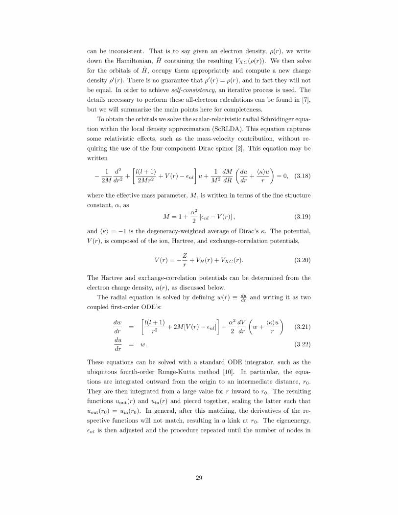
can be inconsistent. That is to say given an electron density, ρ(r), we write

down the Hamiltonian, H containing the resulting VXC(ρ(r)). We then solve

for the orbitals of H, occupy them appropriately and compute a new charge

density ρ′(r). There is no guarantee that ρ′(r) = ρ(r), and in fact they will not

be equal. In order to achieve self-consistency, an iterative process is used. The

details necessary to perform these all-electron calculations can be found in [7],

but we will summarize the main points here for completeness.

To obtain the orbitals we solve the scalar-relativistic radial Schrodinger equa-

tion within the local density approximation (ScRLDA). This equation captures

some relativistic effects, such as the mass-velocity contribution, without re-

quiring the use of the four-component Dirac spinor [2]. This equation may be

written

− 1

2M

d2

dr2+

[l(l + 1)

2Mr2+ V (r)− εnl

]

u+1

M2

dM

dR

(du

dr+〈κ〉ur

)

= 0, (3.18)

where the effective mass parameter, M , is written in terms of the fine structure

constant, α, as

M = 1 +α2

2[εnl − V (r)] , (3.19)

and 〈κ〉 = −1 is the degeneracy-weighted average of Dirac’s κ. The potential,

V (r), is composed of the ion, Hartree, and exchange-correlation potentials,

V (r) = −Zr

+ VH(r) + VXC(r). (3.20)

The Hartree and exchange-correlation potentials can be determined from the

electron charge density, n(r), as discussed below.

The radial equation is solved by defining w(r) ≡ dudr and writing it as two

coupled first-order ODE’s:

dw

dr=

[l(l + 1)

r2+ 2M [V (r)− εnl]

]

− α2

2

dV

dr

(

w +〈κ〉ur

)

(3.21)

du

dr= w. (3.22)

These equations can be solved with a standard ODE integrator, such as the

ubiquitous fourth-order Runge-Kutta method [10]. In particular, the equa-

tions are integrated outward from the origin to an intermediate distance, r0.

They are then integrated from a large value for r inward to r0. The resulting

functions uout(r) and uin(r) and pieced together, scaling the latter such that

uout(r0) = uin(r0). In general, after this matching, the derivatives of the re-

spective functions will not match, resulting in a kink at r0. The eigenenergy,

εnl is then adjusted and the procedure repeated until the number of nodes in

29

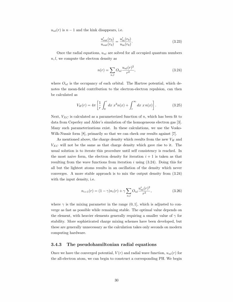
unl(r) is n− 1 and the kink disappears, i.e.

u′out(r0)

uout(r0)=u′in(r0)

uin(r0). (3.23)

Once the radial equations, unl are solved for all occupied quantum numbers

n, l, we compute the electron density as

n(r) =∑

n,l

Onlunl(r)

2

r2, (3.24)

where Onl is the occupancy of each orbital. The Hartree potential, which de-

notes the mean-field contribution to the electron-electron repulsion, can then

be calculated as

VH(r) = 4π

[1

r

∫ r

0

dx x2n(x) +

∫ ∞

r

dx xn(x)

]

. (3.25)

Next, VXC is calculated as a parameterized function of n, which has been fit to

data from Ceperley and Alder’s simulation of the homogeneous electron gas [3].

Many such parameterizations exist. In these calculations, we use the Vosko-

Wilk-Nusair form [8], primarily so that we can check our results against [7].

As mentioned above, the charge density which results from the new VH and

VXC will not be the same as that charge density which gave rise to it. The

usual solution is to iterate this procedure until self consistency is reached. In

the most naive form, the electron density for iteration i + 1 is taken as that

resulting from the wave functions from iteration i using (3.24). Doing this for

all but the lightest atoms results in an oscillation of the density which never

converges. A more stable approach is to mix the output density from (3.24)

with the input density, i.e.

ni+1(r) = (1− γ)ni(r) + γ∑

n,l

Onlui

nl(r)2

r2, (3.26)

where γ is the mixing parameter in the range (0, 1], which is adjusted to con-

verge as fast as possible while remaining stable. The optimal value depends on

the element, with heavier elements generally requiring a smaller value of γ for

stability. More sophisticated charge mixing schemes have been developed, but

these are generally unnecessary as the calculation takes only seconds on modern

computing hardware.

3.4.3 The pseudohamiltonian radial equations

Once we have the converged potential, V (r) and radial wave function, unl(r) for

the all-electron atom, we can begin to construct a corresponding PH. We begin

30

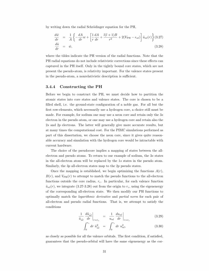
by writing down the radial Schrodinger equation for the PH,

dw

dr=

1

A

−dAdrw +

[1

r

dA

dr+l(l + 1)B

r2+ 2(VPH − εnl)

]

unl(r)

(3.27)

du

dr= w, (3.28)

where the tildes indicate the PH version of the radial functions. Note that the

PH radial equations do not include relativistic corrections since these effects can

captured in the PH itself. Only in the tightly bound core states, which are not

present the pseudo-atom, is relativity important. For the valence states present

in the pseudo-atom, a nonrelativistic description is sufficient.

3.4.4 Constructing the PH

Before we begin to construct the PH, we must decide how to partition the

atomic states into core states and valence states. The core is chosen to be a

filled shell, i.e. the ground-state configuration of a noble gas. For all but the

first row-elements, which necessarily use a hydrogen core, a choice still must be

made. For example, for sodium one may use a neon core and retain only the 3s

electron in the pseudo atom, or one may use a hydrogen core and retain also the

2s and 2p electrons. The latter will generally give more accurate results, but

at many times the computational cost. For the PIMC simulations performed as

part of this dissertation, we choose the neon core, since it gives quite reason-

able accuracy and simulation with the hydrogen core would be intractable with

current hardware.

The choice of the pseudocore implies a mapping of states between the all-

electron and pseudo atoms. To return to our example of sodium, the 3s states

in the all-electron atom will be replaced by the 1s states in the pseudo atom.

Similarly, the 3p all-electron states map to the 2p pseudo states.

Once the mapping is established, we begin optimizing the functions A(r),

B(r), and VPH(r) to attempt to match the pseudo functions to the all-electron

functions outside the core radius, rc. In particular, for each valence function

unl(r), we integrate (3.27-3.28) out from the origin to rc, using the eigenenergy

of the corresponding all-electron state. We then modify our PH functions to

optimally match the logarithmic derivative and partial norm for each pair of

all-electron and pseudo radial functions. That is, we attempt to satisfy the

conditions

1

unl

dunl

dr

∣∣∣∣r=rc

=1

unl

dunl

dr

∣∣∣∣r=rc

(3.29)

∫ rc

0

dr u2nl

=

∫ rc

0

dr u2nl, (3.30)

as closely as possible for all the valence orbitals. The first condition, if satisfied,

guarantees that the pseudo-orbital will have the same eigenenergy as the cor-

31

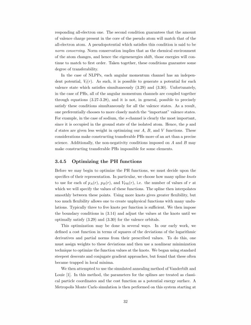
responding all-electron one. The second condition guarantees that the amount

of valence charge present in the core of the pseudo atom will match that of the

all-electron atom. A pseudopotential which satisfies this condition is said to be

norm conserving. Norm conservation implies that as the chemical environment

of the atom changes, and hence the eigenenergies shift, those energies will con-

tinue to match to first order. Taken together, these conditions guarantee some

degree of transferability.

In the case of NLPPs, each angular momentum channel has an indepen-

dent potential, Vl(r). As such, it is possible to generate a potential for each

valence state which satisfies simultaneously (3.29) and (3.30). Unfortunately,

in the case of PHs, all of the angular momentum channels are coupled together

through equations (3.27-3.28), and it is not, in general, possible to precisely

satisfy these conditions simultaneously for all the valence states. As a result,

one preferentially chooses to more closely match the “important” valence states.

For example, in the case of sodium, the s-channel is clearly the most important,

since it is occupied in the ground state of the isolated atom. Hence, the p and

d states are given less weight in optimizing our A, B, and V functions. These

considerations make constructing transferable PHs more of an art than a precise

science. Additionally, the non-negativity conditions imposed on A and B may

make constructing transferable PHs impossible for some elements.

3.4.5 Optimizing the PH functions

Before we may begin to optimize the PH functions, we must decide upon the

specifics of their representation. In particular, we choose how many spline knots

to use for each of pA(r), pB(r), and VPH(r), i.e. the number of values of r at

which we will specify the values of these functions. The spline then interpolates

smoothly between these points. Using more knots gives greater flexibility, but

too much flexibility allows one to create unphysical functions with many undu-

lations. Typically three to five knots per function is sufficient. We then impose

the boundary conditions in (3.14) and adjust the values at the knots until we

optimally satisfy (3.29) and (3.30) for the valence orbitals.

This optimization may be done in several ways. In our early work, we

defined a cost function in terms of squares of the deviations of the logarithmic

derivatives and partial norms from their prescribed values. To do this, one

must assign weights to these deviations and then use a nonlinear minimization

technique to optimize the function values at the knots. We began using standard

steepest descents and conjugate gradient approaches, but found that these often

became trapped in local minima.

We then attempted to use the simulated annealing method of Vanderbilt and

Louie [1]. In this method, the parameters for the splines are treated as classi-

cal particle coordinates and the cost function as a potential energy surface. A

Metropolis Monte Carlo simulation is then performed on this system starting at

32

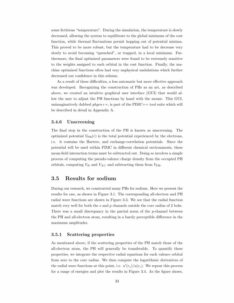
some fictitious “temperature”. During the simulation, the temperature is slowly

decreased, allowing the system to equilibrate to the global minimum of the cost

function, while thermal fluctuations permit hopping out of potential minima.

This proved to be more robust, but the temperature had to be decrease very

slowly to avoid becoming “quenched”, or trapped, in a local minimum. Fur-

thermore, the final optimized parameters were found to be extremely sensitive

to the weights assigned to each orbital in the cost function. Finally, the ma-

chine optimized functions often had very unphysical undulations which further

decreased our confidence in this scheme.

As a result of these difficulties, a less automatic but more effective approach

was developed. Recognizing the construction of PHs as an art, as described

above, we created an intuitive graphical user interface (GUI) that would al-

low the user to adjust the PH functions by hand with the mouse. This GUI,

unimaginatively dubbed phgen++, is part of the PIMC++ tool suite which will

be described in detail in Appendix A.

3.4.6 Unscreening

The final step in the construction of the PH is known as unscreening. The

optimized potential VPH(r) is the total potential experienced by the electrons,

i.e. it contains the Hartree, and exchange-correlation potentials. Since the

potential will be used within PIMC in different chemical environments, these

mean-field interaction terms must be subtracted out. Doing so involves a simple

process of computing the pseudo-valence charge density from the occupied PH

orbitals, computing VH and VXC and subtracting them from VPH.

3.5 Results for sodium

During our research, we constructed many PHs for sodium. Here we present the

results for one, as shown in Figure 3.1. The corresponding all-electron and PH

radial wave functions are shown in Figure 3.3. We see that the radial function

match very well for both the s and p channels outside the core radius of 2 bohr.

There was a small discrepancy in the partial norm of the p-channel between

the PH and all-electron atom, resulting in a barely perceptible difference in the

maximum amplitudes.

3.5.1 Scattering properties

As mentioned above, if the scattering properties of the PH match those of the

all-electron atom, the PH will generally be transferable. To quantify these

properties, we integrate the respective radial equations for each valence orbital

from zero to the core radius. We then compute the logarithmic derivatives of

the radial wave functions at this point, i.e. u′(rc)/u(rc). We repeat this process

for a range of energies and plot the results in Figure 3.4. As the figure shows,

33

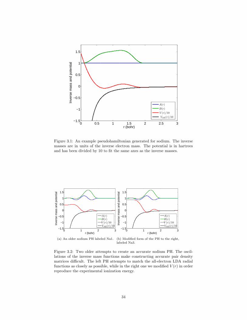
0 0.5 1 1.5 2 2.5 3−1.5

−1

−0.5

0

0.5

1

1.5

r (bohr)

Inve

rse

mas

s an

d po

tent

ial

PSfrag replacementsA(r)

B(r)

V (r)/10

VAE(r)/10

Figure 3.1: An example pseudohamiltonian generated for sodium. The inversemasses are in units of the inverse electron mass. The potential is in hartreesand has been divided by 10 to fit the same axes as the inverse masses.

0 1 2 3−1.5

−1

−0.5

0

0.5

1

1.5

r (bohr)

Inve

rse

mas

s an

d po

tent

ial

PSfrag replacementsA(r)B(r)V (r)/10VAE(r)/10

(a) An older sodium PH labeled Na1.

0 1 2 3−1.5

−1

−0.5

0

0.5

1

1.5

r (bohr)

Inve

rse

mas

s an

d po

tent

ial

PSfrag replacementsA(r)B(r)V (r)/10VAE(r)/10

(b) Modified form of the PH to the right,labeled Na3.

Figure 3.2: Two older attempts to create an accurate sodium PH. The oscil-lations of the inverse mass functions make constructing accurate pair densitymatrices difficult. The left PH attempts to match the all-electron LDA radialfunctions as closely as possible, while in the right one we modified V (r) in orderreproduce the experimental ionization energy.

34

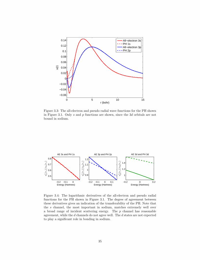
0 5 10 15

−0.06

−0.04

−0.02

0

0.02

0.04

0.06

0.08

0.1

0.12

0.14

r (bohr)

u(r)

All−electron 3sPH 1sAll−electron 3pPH 2p

Figure 3.3: The all-electron and pseudo radial wave functions for the PH shownin Figure 3.1. Only s and p functions are shown, since the 3d orbitals are notbound in sodium.

−0.2 −0.1 0

0.5

0.6

0.7

0.8

AE 3s and PH 1s

Energy (Hartrees)−0.2 −0.1 0 0.1

0.9

1

1.1

1.2

AE 3p and PH 2p

Energy (Hartrees)−0.2 0 0.2

1

1.2

1.4

AE 3d and PH 3d

Energy (Hartrees)

PSfrag replacements

u′ s(r

c)/u

s(r

c)

u′ p(r

c)/u

p(r

c)

u′ d(r

c)/u

d(r

c)

Figure 3.4: The logarithmic derivatives of the all-electron and pseudo radialfunctions for the PH shown in Figure 3.1. The degree of agreement betweenthese derivatives gives an indication of the transferability of the PH. Note thatthe s channel, the most important in sodium, matches extremely well overa broad range of incident scattering energy. The p channel has reasonableagreement, while the d channels do not agree well. The d states are not expectedto play a significant role in bonding in sodium.

35

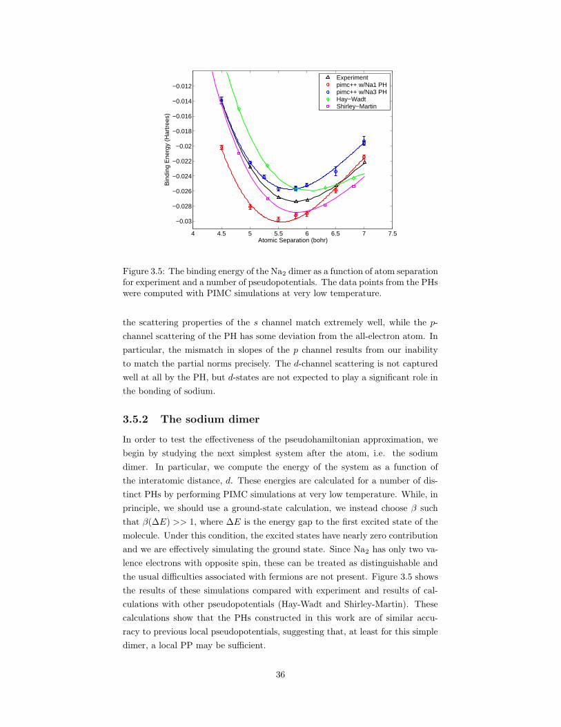
4 4.5 5 5.5 6 6.5 7 7.5

−0.03

−0.028

−0.026

−0.024

−0.022

−0.02

−0.018

−0.016

−0.014

−0.012

Atomic Separation (bohr)

Bin

ding

Ene

rgy

(Har

tree

s)

Experimentpimc++ w/Na1 PHpimc++ w/Na3 PHHay−WadtShirley−Martin

Figure 3.5: The binding energy of the Na2 dimer as a function of atom separationfor experiment and a number of pseudopotentials. The data points from the PHswere computed with PIMC simulations at very low temperature.

the scattering properties of the s channel match extremely well, while the p-

channel scattering of the PH has some deviation from the all-electron atom. In

particular, the mismatch in slopes of the p channel results from our inability

to match the partial norms precisely. The d-channel scattering is not captured

well at all by the PH, but d-states are not expected to play a significant role in

the bonding of sodium.

3.5.2 The sodium dimer

In order to test the effectiveness of the pseudohamiltonian approximation, we

begin by studying the next simplest system after the atom, i.e. the sodium

dimer. In particular, we compute the energy of the system as a function of

the interatomic distance, d. These energies are calculated for a number of dis-

tinct PHs by performing PIMC simulations at very low temperature. While, in

principle, we should use a ground-state calculation, we instead choose β such

that β(∆E) >> 1, where ∆E is the energy gap to the first excited state of the

molecule. Under this condition, the excited states have nearly zero contribution

and we are effectively simulating the ground state. Since Na2 has only two va-

lence electrons with opposite spin, these can be treated as distinguishable and

the usual difficulties associated with fermions are not present. Figure 3.5 shows

the results of these simulations compared with experiment and results of cal-

culations with other pseudopotentials (Hay-Wadt and Shirley-Martin). These

calculations show that the PHs constructed in this work are of similar accu-

racy to previous local pseudopotentials, suggesting that, at least for this simple

dimer, a local PP may be sufficient.

36

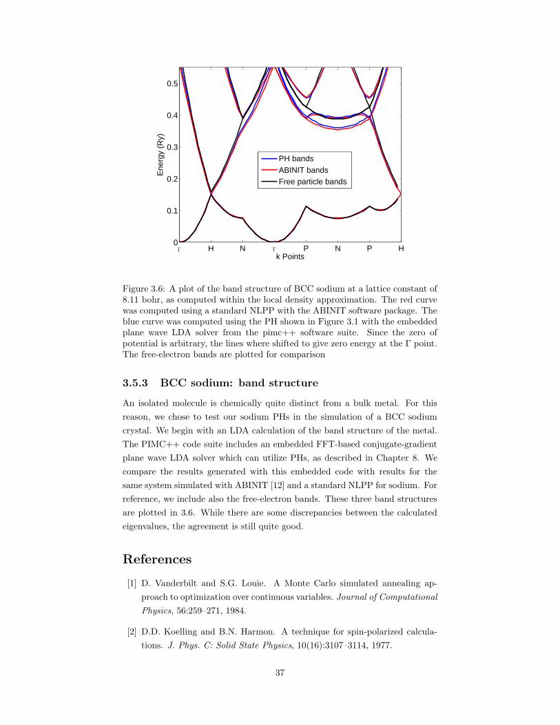
H N P N P H0

0.1

0.2

0.3

0.4

0.5

k Points

Ene

rgy

(Ry)

PH bands

ABINIT bands

Free particle bands

PSfrag replacementsΓΓ

Figure 3.6: A plot of the band structure of BCC sodium at a lattice constant of8.11 bohr, as computed within the local density approximation. The red curvewas computed using a standard NLPP with the ABINIT software package. Theblue curve was computed using the PH shown in Figure 3.1 with the embeddedplane wave LDA solver from the pimc++ software suite. Since the zero ofpotential is arbitrary, the lines where shifted to give zero energy at the Γ point.The free-electron bands are plotted for comparison

3.5.3 BCC sodium: band structure

An isolated molecule is chemically quite distinct from a bulk metal. For this

reason, we chose to test our sodium PHs in the simulation of a BCC sodium

crystal. We begin with an LDA calculation of the band structure of the metal.

The PIMC++ code suite includes an embedded FFT-based conjugate-gradient

plane wave LDA solver which can utilize PHs, as described in Chapter 8. We

compare the results generated with this embedded code with results for the

same system simulated with ABINIT [12] and a standard NLPP for sodium. For

reference, we include also the free-electron bands. These three band structures

are plotted in 3.6. While there are some discrepancies between the calculated

eigenvalues, the agreement is still quite good.

References

[1] D. Vanderbilt and S.G. Louie. A Monte Carlo simulated annealing ap-

proach to optimization over continuous variables. Journal of Computational

Physics, 56:259–271, 1984.

[2] D.D. Koelling and B.N. Harmon. A technique for spin-polarized calcula-

tions. J. Phys. C: Solid State Physics, 10(16):3107–3114, 1977.

37

[3] D.M. Ceperley and B.J. Alder. Ground State of the Electron Gas by a

Stochastic Method. Phys. Rev. Lett., 45(7):566, 18 August 1980.

[4] G.B. Bachelet, D.M. Ceperley, and M.G.B. Chiochetti. Novel Psuedo-

Hamiltonian for Quantum Monte Carlo Simulations. Physical Review Let-

ters, 62(18):2088–2091, 1 May 1989.

[5] John G. Herriot and Christian H. Reinsch. ALGORITHM 600: Translation

of Algorithm 507: Procedures for Quintic Natural Spline Interpolation.

ACM Transactions on Mathematical Software, 9(2):258–259, June 1983.

[6] Lubos Mitas, Eric L. Shirley, and David M. Ceperley. Nonlocal pseudopo-

tentials and diffusion Monte Carlo. J. Chem. Phys., 95(5):3467–3475, 1

September 1991.

[7] S. Kotochigova, Z.H. Levine, E.L. Shirley, M.D. Stiles, and C.W. Clark.

Local-density-functional calculations of the energy of atoms. Phys. Rev. A,

55:191, 1997.

[8] S.H. Vosko, L. Wilk, and M. Nusair. Can. J. Phys., 58:1200, 1980.

[9] Warren E. Pickett. Pseudopotential methods in condensed matter applica-

tions. Computer Physics Reports, 9:115–198, 1989.

[10] William H. Press, Saul A. Teukolsky, William T. Vetterling, and Brian P.

Flannery. Numerical Recipes in C, chapter 16, pages 710–714. Cambridge

University Press, 1992.

[11] W.M.C. Foulkes and M. Schluter. Pseudopotentials with position-

dependent masses. Physical Review B, 42(18):11505–11529, 15 December

1990.

[12] X. Gonze, J.M. Beuken, R. Caracas, F. Detraux, M. Fuchs, G.M. Rig-

nanese, L. Sindic, M. Verstraete, G. Zerah, F. Jollet, M. Torrent, A. Roy,

M. Mikami, Ph. Ghosez, J.Y. Raty, and D.C. Allan. First-principles compu-

tation of material properties : the ABINIT software project. Computational

Materials Science, 25:478–492, 2002.

38

Chapter 4

Computing pair densitymatrices

4.1 The density matrix squaring method

In Chapter 2, we introduced the matrix squaring property of the density matrix.

In this chapter, we explain how this property may be used to calculate the

density matrix for a pair of particles interacting via a central potential. This

method was first introduced by Storer in 1968 for the Coulomb potential [4]

and was later generalized by Klemm and Storer to all central potentials [1].

The authors used numerical methods that were appropriate for the hardware

of the time. Here, we introduce many improvements to the original method in

order to achieve much higher accuracy. We also modify the method to work

with pseudohamiltonians through the use of a novel coordinate transform. As

we shall see, PHs significantly complicate the matter, but with persistence, we

find it possible to compute accurate density matrices from them. Most of this

material has not been published elsewhere, but is quite important to the PIMC

method.

We should note that a slight modification to the matrix squaring approach

has been proposed by Schmidt and Lee [2]. Colleagues have reported that it is

effective for central potentials, but we have not implemented it. It should be

possible to modify the method to work with pseudohamiltonians in a manner

similar to what is presented below.

4.1.1 The pair density matrix

Naively, the density matrix for two particles in three dimensions has twelve

spatial dimensions, i.e. r1, r2, r′1, r

′2. For particles interacting via a central

potential, however, the density matrix can be written in terms of their relative

coordinates, ρ(r, r′; τ), where r ≡ r2 − r1 and r′ ≡ r′2 − r′1. Since the potential

depends only on the distance between the particles (and not their relative orien-

tation), the spatial dimensionality can be further reduced to three, namely |r|,|r′|, and cos(θ) ≡ (r · r′)/|r||r′|. Because of this reduction, it is possible to store

the density matrix explicitly in a table, and later interpolate its value during

PIMC simulation.

The matrix squaring property, 2.6, states that given a density matrix at

temperature T , we may compute the density at temperature T/2 by squaring

39

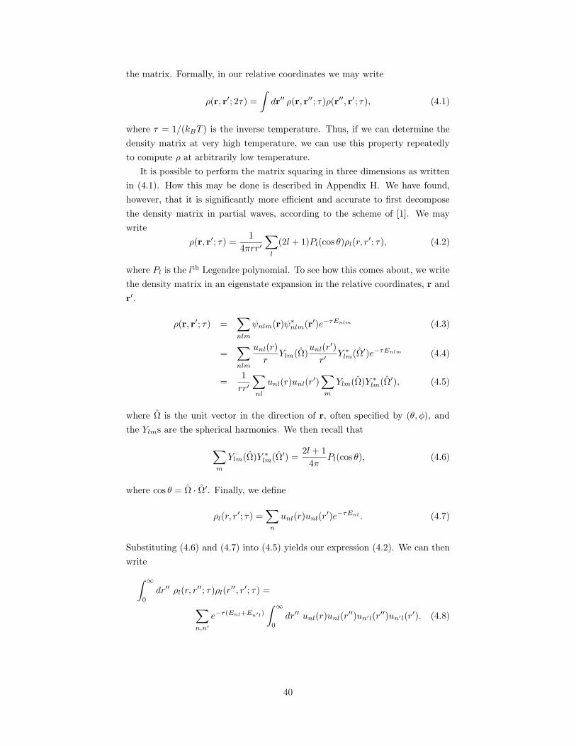
the matrix. Formally, in our relative coordinates we may write

ρ(r, r′; 2τ) =

∫

dr′′ ρ(r, r′′; τ)ρ(r′′, r′; τ), (4.1)

where τ = 1/(kBT ) is the inverse temperature. Thus, if we can determine the

density matrix at very high temperature, we can use this property repeatedly

to compute ρ at arbitrarily low temperature.

It is possible to perform the matrix squaring in three dimensions as written

in (4.1). How this may be done is described in Appendix H. We have found,

however, that it is significantly more efficient and accurate to first decompose

the density matrix in partial waves, according to the scheme of [1]. We may

write

ρ(r, r′; τ) =1

4πrr′

∑

l

(2l + 1)Pl(cos θ)ρl(r, r′; τ), (4.2)

where Pl is the lth Legendre polynomial. To see how this comes about, we write

the density matrix in an eigenstate expansion in the relative coordinates, r and

r′.

ρ(r, r′; τ) =∑

nlm

ψnlm(r)ψ∗nlm(r′)e−τEnlm (4.3)

=∑

nlm

unl(r)

rYlm(Ω)

unl(r′)

r′Y ∗

lm(Ω′)e−τEnlm (4.4)

=1

rr′

∑

nl

unl(r)unl(r′)∑

m

Ylm(Ω)Y ∗lm(Ω′), (4.5)

where Ω is the unit vector in the direction of r, often specified by (θ, φ), and

the Ylms are the spherical harmonics. We then recall that

∑

m

Ylm(Ω)Y ∗lm(Ω′) =

2l + 1

4πPl(cos θ), (4.6)

where cos θ = Ω · Ω′. Finally, we define

ρl(r, r′; τ) =

∑

n

unl(r)unl(r′)e−τEnl . (4.7)

Substituting (4.6) and (4.7) into (4.5) yields our expression (4.2). We can then

write

∫ ∞

0

dr′′ ρl(r, r′′; τ)ρl(r

′′, r′; τ) =

∑

n,n′

e−τ(Enl+En′l)

∫ ∞

0

dr′′ unl(r)unl(r′′)un′l(r

′′)un′l(r′). (4.8)

40

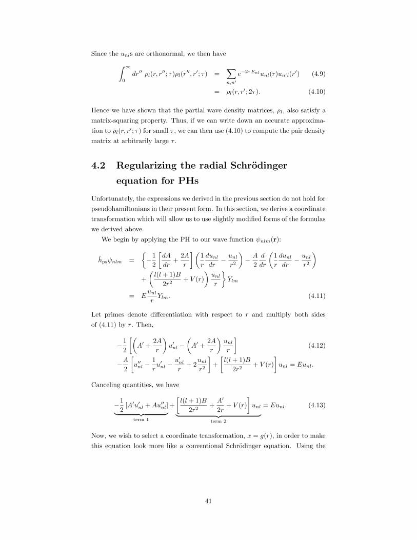
Since the unls are orthonormal, we then have

∫ ∞

0

dr′′ ρl(r, r′′; τ)ρl(r

′′, r′; τ) =∑

n,n′

e−2τEnlunl(r)un′l(r′) (4.9)

= ρl(r, r′; 2τ). (4.10)

Hence we have shown that the partial wave density matrices, ρl, also satisfy a

matrix-squaring property. Thus, if we can write down an accurate approxima-

tion to ρl(r, r′; τ) for small τ , we can then use (4.10) to compute the pair density

matrix at arbitrarily large τ .

4.2 Regularizing the radial Schrodinger

equation for PHs

Unfortunately, the expressions we derived in the previous section do not hold for

pseudohamiltonians in their present form. In this section, we derive a coordinate

transformation which will allow us to use slightly modified forms of the formulas

we derived above.

We begin by applying the PH to our wave function ψnlm(r):

hpsψnlm =

−1

2

[dA

dr+

2A

r

](1

r

dunl

dr− unl

r2

)

− A

2

d

dr

(1

r

dunl

dr− unl

r2

)

+

(l(l + 1)B

2r2+ V (r)

)unl

r

Ylm

= Eunl

rYlm. (4.11)

Let primes denote differentiation with respect to r and multiply both sides

of (4.11) by r. Then,

−1

2

[(

A′ +2A

r

)

u′nl −(

A′ +2A

r

)unl

r

]

(4.12)

−A2

[

u′′nl −1

ru′nl −

u′nl

r+ 2

unl

r2

]

+

[l(l + 1)B

2r2+ V (r)

]

unl = Eunl.

Canceling quantities, we have

−1

2[A′u′nl +Au′′nl]

︸ ︷︷ ︸

term 1

+

[l(l + 1)B

2r2+A′

2r+ V (r)

]

unl

︸ ︷︷ ︸

term 2

= Eunl. (4.13)

Now, we wish to select a coordinate transformation, x = g(r), in order to make

this equation look more like a conventional Schrodinger equation. Using the

41

chain rule, we have

dunl

dr=

dunl

dx

dx

dr(4.14)

d2unl

dr2=

d2unl

dx2

(dx

dr

)2

+dunl

dx

d2x

dr2. (4.15)

Considering the first term of (4.13),

term 1 = −1

2

[

dunl

dx

dA

dr

dx

dr+A

d2unl

dx2

(dx

dr

)2

+Adunl

dx

d2x

dr2

]

. (4.16)

For convenience let dots represent differentiation with respect to x, that is,

A = dAdx . We wish to reduce our Schrodinger equation to one resembling a

standard radial Schrodinger equation with a fixed electron mass. We see that

we can make a stride toward this goal by setting

dx

dr≡ A− 1

2 ,d2x

dr2= −1

2A− 3

2A′. (4.17)

Then

term 1 = −1

2

[

A− 12A′unl + unl −

1

2A− 1

2A′unl

]

= −1

2

[

unl +1

2A− 1

2A′unl

]

. (4.18)

Now, we wish to eliminate the unl term with another transformation. Define

unl ≡ Aαqnl, (4.19)

which implies that

unl = αAα−1Aqnl +Aαqnl (4.20)

= αAα− 12A′qnl +Aαqnl.

Inserting these into (4.18), we have

unl = α

(

α− 1

2

)

Aα− 32 AA′qnl + αAα− 1

2 A′qnl + αAα− 12A′qnl (4.21)

+αAα−1Aqnl +Aαqnl

= α

(

α− 1

2

)

Aα−1(A′)2qnl + αAαA′′qnl + αAα− 12A′qnl

+αAα− 12A′qnl +Aαqnl

=

[

α

(

α− 1

2

)

Aα−1(A′)2 + αAαA′′]

qnl + 2αAα− 12A′qnl +Aαqnl.

42

Substituting these expressions yields

term 1 = −1

2

[

α

(

α− 1

2

)

Aα−1(A′)2 + αAαA′′ +1

2αAα−1(A′)2

]

qnl

+

(

2αAα− 12A′ +

1

2Aα− 1

2A′)

qnl +Aαqnl

(4.22)

= −1

2

[α2Aα−1(A′)2 + αAαA′′] qnl

+

(

2α+1

2

)(

Aα− 12A′)

qnl +Aαqnl

.

We see from the above expression that if we set α = − 14 , the coefficient of the

qnl term will vanish. Making this substitution,

term 1 = −1

2

[1

16A− 5

4 (A′)2 − 1

4A− 1

4A′′]

qnl +A− 14 qnl

. (4.23)

Now, we rewrite our full radial Schrodinger equation, multiplying both sides of

the equation by A14 ,

− 1

2qnl +

[l(l + 1)B

2r2+A′

2r− 1

32

(A′)2

A+A′′

8+ V (r)− Enl

]

qnl = 0. (4.24)

We then make the definition that

Wl(r) ≡l(l + 1)B(r)

2r2+A′

2r− (A′)2

32A+A′′

8+ V (r). (4.25)

Then, our transformed radial equation becomes

− 1

2

d2qnl

dx2+ [Wl(r)− Enl] qnl = 0, (4.26)

which has the same form as the radial equation for a central potential, with the

transformed radial Hamiltonian given by

Hl = −1

2

d2

dx2+Wl(r(x)). (4.27)

Implementing the coordinate transform

We recall that dxdr = A(r)−

12 . Then

x(r) = x0 +

∫ r

0

dr′ A− 12 (r′) (4.28)

Since A(r) > 0 for all r, this expression establishes a one-to-one mapping be-

tween r and x. In order that we may keep the limits of integration in our later

expressions to be from 0 to ∞, we must have x(0) = 0, which implies that

x0 = 0. Thus,

x(r) ≡∫ r

0

dr′ A− 12 (r′). (4.29)

43

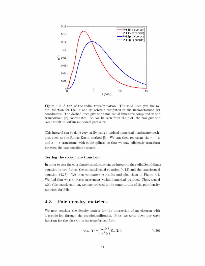
0 5 10 150

0.02

0.04

0.06

0.08

0.1

0.12

0.14

0.16

r (bohr)

u(r)

PH 1s (r coords)PH 1s (x coords)PH 2p (r coords)PH 2p (x coords)

Figure 4.1: A test of the radial transformation. The solid lines give the ra-dial function for the 1s and 2p orbitals computed in the untransformed (r)coordinates. The dashed lines give the same radial functions computed in thetransformed (x) coordinates. As can be seen from the plot, the two give thesame result to within numerical precision.

This integral can be done very easily using standard numerical quadrature meth-

ods, such as the Runge-Kutta method [5]. We can then represent the r → x

and x → r transforms with cubic splines, so that we may efficiently transform

between the two coordinate spaces.

Testing the coordinate transform

In order to test the coordinate transformation, we integrate the radial Schrodinger

equation in two forms: the untransformed equation (4.13) and the transformed

equation (4.27). We then compare the results and plot them in Figure 4.1.

We find that we get precise agreement within numerical accuracy. Thus, armed

with this transformation, we may proceed to the computation of the pair density

matrices for PHs.

4.3 Pair density matrices

We now consider the density matrix for the interaction of an electron with

a pseudo-ion through the pseudohamiltonian. First, we write down our wave

function for the electron in its transformed form,

ψnlm(r) =qnl(r)

rA14 (r)

Ylm(Ω). (4.30)

44

We can then write the pair density matrix for the PH as

ρ(r, r′;β) =∑

nlm

ψnlm(r)ψ∗nlm(r′)e−βEnlm (4.31)

=1

rr′A14 (r)A

14 (r′)

∑

nl

qnl(r)qnl(r′)∑

m

Ylm(Ω)Y ∗lm(Ω′).

Using (4.6), we can write

ρ(r, r′;β) =1

4πrr′(AA′)14

∑

l

(2l + 1)Pl(cos θ)∑

n

qnlq′nle

−βEnl . (4.32)

Hence, we define now define our transformed PH partial wave density matrix as

ρl(x, x′;β) =

∑

n

qnl(x)q∗nl(x

′)e−βEnl , (4.33)

so that the final pair density matrix can be expanded as

ρ(r, r′;β) =1

4πrr′(AA′)14

∑

l

(2l + 1)Pl(cos θ)ρl(x, x′;β). (4.34)

The squaring property in transformed coordinates

Since qnl satisfies (4.26), then it also satisfies the orthogonality condition,

∫ ∞

0

dx qnl(x)q∗pl(x) = δnp. (4.35)

Hence, we can write

∫ ∞

0

dx′′ρl(x, x′′;β) ρl(x

′′, x′;β)

=

∫ ∞

0

dx′′∑

n,p

qnl(x)q∗nl(x

′′)qpl(x′′)q∗pl(x

′)e−β(Enl+Epl)

=∑

n,p

qnl(x)q∗pl(x

′)e−β(Enl+Epl)δnp

=∑

n

qnl(x)q∗nl(x

′)e−2βEnl

= ρl(x, x′; 2β). (4.36)

Thus, the squaring property we introduced above also holds in the transformed

x coordinates.

4.4 The high-temperature approximation

The matrix squaring expression in (4.36) is useless without a starting point. In

this section we address how we may approximate ρl at high temperature (small

β) in order to initialize the squaring sequence.

45

We begin with our sum-over-states expression for ρl,

ρl(x, x′;β) =

∑

n

qnl(x)q∗nl(x

′)e−βEnl . (4.37)

Since qnl(x) is an eigenvector of Hl, defined as

Hl = −1

2

d2

dx2+Wl(r), (4.38)

then

e−βHlqnl = e−βEnlqnl. (4.39)

Thus, we may write

ρl(x, x′;β) =

∑

n

[

e−βHlqnl(x)]

q∗nl(x′)

=∑

n

⟨

x∣∣∣e−βHl

∣∣∣ qnl

⟩

〈qnl|x′〉

=⟨

x∣∣∣e−βHl

∣∣∣x′⟩

. (4.40)

Now, we break up Hl into two pieces,

Hl = H0l + H1

l , (4.41)

which do not commute. We then make the approximation that

e−βHl ≈ e−βH1

l2 e−βH0

l e−βH1

l2 . (4.42)

This approximation has an error of order O(β2). Consider the breakup in which

H0l = −1

2

d2

dx2+l(l + 1)B(0)

2A(0)x2, H1

l = Wl(r)−l(l + 1)B(0)

2A(0)x2≡ Yl(r). (4.43)

The reason for this choice for the breakup will be made clear presently. Recall

that

Wl(r) ≡l(l + 1)B(r)

2r2+A′

2r− (A′)2

32A+A′′

8+ V (r). (4.44)

Thus,

Yl(r) = l(l + 1)

[B(r)

2r2− B(0)

2A(0)x2

]

+A′

2r− (A′)2

32A+A′′

8+ V (r). (4.45)

In constructing our PH, we require that

dB

dr

∣∣∣∣r=0

= 0→ dB

dx

∣∣∣∣x=0

= 0 (4.46)

46

and furthermore that

dA

dr

∣∣∣∣r=0

= 0→ dA

dx

∣∣∣∣x=0

= 0. (4.47)

This implies that, near the origin, r = A(0)12 x. Therefore, for small r,

Yl(r) = l(l + 1)

[(B(0) +B′′(0)r2 + . . . )

(A(0) +A′′(0)r2 + . . . )x2− B(0)

2A(0)x2

]

+ . . . (4.48)

We note that Yl(r), unlike Wl(r), has no centrifugal divergence at the origin.

This property will stabilize the squaring calculation considerably.

4.4.1 Free particle ρ

Now, we turn our attention to H0l , writing

H0l = − d2

dx2+l(l + 1)

2x2. (4.49)

This Hamiltonian has a closed-form l-channel density matrix:

ρ0l (x, x

′;β) = (2πβ)−32 4πxx′ exp

(

−x2 + x′2

2β

)

il

(xx′

β

)

, (4.50)

where il(z) is the modified spherical Bessel function of order l. Note that in our

construction of the pseudohamiltonian, we required that B(0) = A(0), so that

this form is adequate. However, we can, in fact, generalize to the case in which

A(0) 6= B(0), by defining l′, such that

l′(l′ + 1) =B(0)

A(0)l(l + 1). (4.51)

Then,

l′ =

√

1 + 4B(0)A(0) l(l + 1)− 1

2. (4.52)

We may then use a form for il′ which is analytically continued from integer

values to real values. To evaluate il′ , we must use

il′(z) =√

π/(2z)Il′+1/2(z), (4.53)

where Iν(z) is a regular, modified Bessel function of fractional order. For com-

putational purposes, we actually compute a scaled version of this function,

Mν(z) exp(|z|) ≡ Iν(z) (4.54)

47

Putting these expression together, we have

ρ0l (x, x

′;β) = (2πβ)−32 4πxx′ exp

[

− (x− x′)22β

]√

πβ

2xx′Ml′+ 1

2

(xx′

β

)

=

√xx′

βexp

[

− (x− x′)22β

]

Ml′+ 12

(xx′

β

)

. (4.55)

4.4.2 The β-derivative

The derivative of the density matrix with respect to β is needed for the esti-

mator we will use for the total energy in the PIMC simulation. We address its

calculation here. Clearly,

∂

∂βρ(r, r′;β) =

∂

∂β

1

4πrr′(AA′)14

∑

l

(2l + 1)Pl(cos θ)ρl(x, x′;β)

=1

4πrr′(AA′)14

∑

l

(2l + 1)Pl(cos θ)∂

∂βρl(x, x

′;β). (4.56)

We begin with the squaring property,

ρl(x, x′; 2β) =

∫ ∞

0

dx′′ ρl(x, x′′;β)ρl(x

′′, x′;β). (4.57)

Differentiating, we obtain

∂ρl(x, x′; τ)

∂τ

∣∣∣∣τ=2β

=1

2

∂

∂βρl(x, x

′; 2β) (4.58)

=1

2

∫ ∞

0

dx′′ . . .

[

ρl(x, x′′;β)

∂ρ(x′, x′′;β)

∂β+∂ρ(x, x′′;β)

∂βρl(x

′, x′′;β)

]

.

Now, let us define Ul(x, x′;β) by the expression

ρl(x, x′;β) ≡ ρ0

l (x, x′;β)e−Ul(x,x′;β) (4.59)

Then we can write the β-derivative as

∂ρl(x, x′;β)

∂β= e−Ul(x,x′β)

[

∂ρ0l (x, x

′;β)

∂β− ρ0

l (x, x′;β)

∂Ul(x, x′;β)

∂β

]

. (4.60)

Inverting this equation gives

∂Ul(x, x′;β)

∂β=

1

ρ0l (x, x

′;β)

[∂ρ0

l (x, x′;β)

∂β− eUl(x,x′;β) ∂ρl(x, x

′;β)

∂β

]

=eUl(x,x′;β)

ρ0l (x, x

′;β)

[

e−Ul(x,x′;β) ∂ρ0l (x, x

′;β)

∂β− ∂ρl(x, x

′;β)

∂β

]

.

(4.61)

48

Let us now define, for convenience, the ratio

C(x, x′;β) ≡∂ρ0

l (x,x′;β)∂β

ρ0l (x, x

′;β). (4.62)

Now, we may write,

∂Ul(x, x′; τ)

∂τ

∣∣∣∣∣τ=2β

=eUl(x,x′;2β)

ρ0l (x, x

′; 2β)

[

e−Ul(x,x′;2β) ∂ρ0l (x, x

′; τ)

∂τ

∣∣∣∣2β

− ∂ρl(x, x′; τ)

∂τ

∣∣∣∣2β

]

= −eUl(x,x′;2β)

∂ρl(x,x′;τ)∂τ

∣∣∣τ=2β

ρ0l (x, x

′; 2β)− e−Ul(x,x′;2β)C(x, x′; 2β)

︸ ︷︷ ︸

α(x,x′;2β)

.

(4.63)

Furthermore,

∂ρl(x, x′;β)

∂τ

∣∣∣∣τ=2β

=1

2

∫ ∞

0

dx′′ e−[Ul(x,x′′;β)+Ul(x′,x′′;β)]ρ0

l (x, x′′;β)ρ0

l (x′, x′′;β)

×[

C(x, x′′;β) + C(x′, x′′;β)− ∂Ul(x, x′′;β)

∂β− ∂Ul(x

′, x′′;β)

∂β

]

. (4.64)

And, finally,

α(x, x′; 2β) =1

2

∫ ∞

0

dx′′ e−[Ul(x,x′′;β)+Ul(x′,x′′;β)] ρ

0l (x, x

′′;β)ρ0l (x

′, x′′;β)

ρ0l (x, x

′; 2β)

×[

C(x, x′′;β) + C(x′, x′′;β)− 2C(x, x′; 2β)− ∂Ul(x, x′′;β)

∂β− ∂Ul(x

′, x′′;β)

∂β

]

.

(4.65)

Thus, we may square the β-derivative of ρl down from high temperature in a

very similar way to ρl itself.

In order to calculate these quantities we will need to calculate ∂∂β ρ

0l (x, x

′;β).

We undertake this task here. Recall that

ρ0l (x, x

′;β) = (2πβ)−32 4πxx′ exp

(

− (x− x′)22β

)

ml

(xx′

β

)

, (4.66)

where ml(z) ≡ il(z)e−|z| and z ≡ xx′

β . Then, we compute the β derivative as

∂ρ0l (x, x

′;β)

∂β=4πxx′(2πβ)−

32 exp

(

− (x− x′)22β

)

× 1

β

[x2 + x′2

2β− 3

2

]

ml(z)−xx′

βm′

l(z)

.

(4.67)

Here m′l(z) = dil

dz exp(−|z|). Formulas for calculating dil

dz can be found in Sec-

49

tion 4.6. We can now write an explicit expression for C(x, x′;β).

C(x, x′;β) =1

β

[x2 + x′2

2β− 3

2− zm

′l(z)

ml(z)

]

, (4.68)

where z ≡ xx′

β .

4.5 Implementation issues

In this section, we address the numerical issues which must be considered in

order to be able to calculate ρ(r, r′;β) accurately.

4.5.1 Interpolation and partial-wave storage

In order to perform the integrations involved in the squaring of the ρl’s, we

must be able to interpolate the function for arbitrary values of x′′. At high

temperature, the function ρl(x, x′;β) is sharply peaked near the diagonal (x =

x′). Rather than creating an unusual two-dimensional grid peaked along the

diagonal, we choose to represent the function as a product of two pieces,

ρl(x, x′;β) ≡ ρ0

l (x, x′;β)e−Ul(x,x′;β). (4.69)

The part of this function responsible for the peak along the diagonal, ρ0l (x, x

′;β),

has an exact analytic expression. We may thus tabulate and interpolate only

Ul(x, x′;β), which has a much smoother form than the whole ρl. When we

perform the integrations involved in squaring, we use the analytic form of

ρ0l (x, x

′;β), while we numerically interpolate Ul(x, x′;β). After a squaring inte-

gration, we divide the result by ρ0l (x, x

′; 2β) and take the logarithm, and thus

store Ul(x, x′; 2β) for the next iteration.

4.5.2 Evaluating the integrand

The integrand used in the squaring procedure takes on values which can span

many orders of magnitude. As such, it is critical to take great care when com-

puting the integrand. Experience has shown that direct, naive implementation

of the formulas given above yields extremely poor numerical accuracy.

The squaring procedure is usually started at very high temperature, on the

order of 10−6 Hartree−1. Thus, the exponentials involved in the free particle

density matrix in the integrand may take on values which are not representable

as standard 64-bit IEEE double precision floating point numbers. We begin by

reformulating the product

ρl(x, x′′;β)ρl(x

′′, x′;β) = ρ0l (x, x

′′;β)ρ0l (x

′′, x′;β)

× exp

−[

Ul(x, x′′;β) + Ul(x

′′, x′;β]

.(4.70)

50

After we complete the integration, we will divide by ρ0l (x, x

′; 2β) and take the

logarithm in order to compute Ul(x, x′; 2β). We thus consider the quantity

I(r, r′, r′′;β) ≡ ρ0l (x, x

′′;β)ρ0l (x

′′, x′;β)

ρ0l (x, x

′; 2β). (4.71)

We define I ≡ EF and evaluate the terms separately. I ≡ EF .

E =exp

[

− (x−x′′)2

2β

]

exp[

− (x′−x′′)2

2β

]

exp[

− (x−x′)2

4β

] (4.72)

F =

√xx′

βx′′

β Ml′+ 12

(xx′′

β

)

Ml′+ 12

(x′x′′

β

)

√xx′

2β Ml′+ 12

(xx′

2β

) , (4.73)

or, alternatively, F may be written as

F =4πx′′2(πβ)−

32ml

(xx′′

β

)

ml

(x′x′′

β

)

ml

(xx′

2β

) . (4.74)

We work a bit on the exponential part, writing

E =exp

[

−x2+x′2+2x′′2−2x′′(x+x′)2β

]

exp[

− (x−x′)2

4β

] , (4.75)

and define x ≡ x+x′

2 . Then we have,

E =exp

[

−x2+x′2

2β

]

exp[

−x′′2−2x′′xβ

]

exp[

− (x−x′)2

4β

] (4.76)

=exp

[

−x2+x′2

2β

]

exp[

− (x′′−x)2

β

]

exp[

x2

β

]

exp[

− (x−x′)2

4β

] (4.77)

= exp

[

− (x′′ − x)2β

]

. (4.78)

Now we return to the remaining term of the product:

F =2x′′

β

Ml′+ 12

(xx′′

β

)

Ml′+ 12

(x′x′′

β

)

Ml′+ 12

(x′x′

2β

) ; (4.79)

I =2x′′

β

Ml′+ 12

(xx′′

β

)

Ml′+ 12

(x′x′′

β

)

Ml′+ 12

(x′x′

2β

) exp

[

− (x′′ − x)2β

]

. (4.80)

When the temperature is very high, the integrand will become very sharply

51

peaked around x′′ = x. This can cause problems during integration since there

will not be enough accuracy in the floating-point representation of x′′. There-

fore, we make the definition,

s ≡ x′′ − x, (4.81)

and rewrite the integration to be over s, rather than x′′. This will eliminate the

representability problem.

The β-derivative integrand

In this section, we go about manipulating the integrand in equation (4.65) to

make it more computationally tractable. The first line of the integrand is pre-

cisely that from the action integrand, so here we focus on the second line. Define

y ≡ xx′′

β(4.82)

y′ ≡ x′x′′

β(4.83)

z ≡ xx′

2β. (4.84)

In terms of these quantities, we can then write

C(x, x′′;β) + C(x′, x′′;β)− 2C(x, x′; 2β) =

1

β

[x2 + x′2 + 4x′′2

4β− 3

2− ym

′l(y)

ml(y)− y′m

′l(y

′)

ml(y′)+ z

m′l(z)

ml(z)

]

.(4.85)

From Abramowitz and Stegun,

m′l(z) = ml+1(z) +

l

zml(z). (4.86)

Then

zm′

l(z)

ml(z)= z

ml+1(z)

ml(z)+ l (4.87)

C(x, x′′;β) + C(x′, x′′;β)− 2C(x, x′;β) =

1

β

[x2 + x′2 + 4x′′2

4β−(

l +3

2

)

− yml+1(y)

ml(y)− y′ml+1(y

′)

ml(y′)+ z

ml+1(z)

ml(z)

]

.

(4.88)

Asymptotic form

Evaluating the Bessel functions at large values of their arguments can limit the

accuracy of the integration. Here, we consider the asymptotic form of the ratios

in (4.88) to increase both speed and accuracy.

It can be shown that the form of the ratio above can be given as

limz→∞

zml+1(z)

ml(z)= z − (l + 1) + α(z−1 + z−2) + γz−3 + εz−4 +O(z−5), (4.89)

52

where

α =l(l + 1)

2(4.90)

γ = − l(l − 2)(l + 1)(l + 3)

8(4.91)

ε = − l(l + 1)(l2 + l − 3)

2. (4.92)

The error in this goes approximately as e−2z. Using this expression, we can

rewrite (4.88) to obtain

C(x, x′′;β) + C(x′, x′′;β)− 2C(x, x′;β) ≈ 1

β

[(x′′ − x)2

β− 1

2

]

+2αδ

xx′x′′+

4βγ

x2x′2x′′2

[

δ(x′′ + x) +xx′

2

]

+ε

β

[

− y−4 − y′−4 + z−4

]

. (4.93)

4.5.3 Performing the integrals

Now that we have massaged the integrands for the actions into numerically

well-behaved forms, we must set about performing the integrations. We begin

by writing the formula for the squared action as

Ul(x, x′; 2β) =

− log

∫ s2

s1

ds I(x, x′s;β) exp[

−U(x, s+ x;β) + U(s+ x, x′;β)]

, (4.94)

where I is now written

I(x, x′, s;β) =2(s+ x)

β

Ml′+ 12

(x(s+x)

β

)

Ml′+ 12

(x′(s+x)

β

)

Ml′+ 12

(x′x′

2β

) exp

[−s2β

]

. (4.95)

In principle, the integration limits should be chosen such that the integral over

x′′ be from 0 to ∞, i.e. that s1 = −x and s2 = ∞. In practice, the gaus-

sian factor e−s2/β kills off the integrand sufficiently quickly that only a finite

integration domain is needed.

Hermite integration

For large x, I(x, x′, s;β) takes on the asymptotic form e−s2/β . For potentials

which are smooth far from the origin, the integrand will then be dominated by

this gaussian factor, but will be modulated somewhat by the potential action

factors. Hermite quadrature is optimized to numerically evaluate integrals of

precisely this form [3]. The integration is written as

∫ ∞

−∞dx f(x)e−x2 ≈

∑

i

wif(xi)e−x2

i , (4.96)

53

where the sum is over an N -point quadrature rule with abscissas, xi, each of

which are given by the ith zero of Hn(x), and weights, wi, which are given by

wi =2N−1N !

√πex2

i

N2 [HN−1(xi)]2 . (4.97)

For convenience, we have computed these weights to high accuracy and included

a number of rules in Appendix J. Hermite integration is very fast and accurate

and is ideally suited for our purpose here.

Gauss-Kronrod adaptive integration

Near the origin, the Bessel function contributions to I are significant and the

integrand no longer takes the form of a modulated gaussian. As a result, Her-

mite quadrature is inappropriate. Instead, in these regions, we use an adaptive

integration method with quadrature rules known as Gauss-Kronrod [6]. In the

method, we first use an n-point rule to approximate the integral. We then es-

timate the error using a (2n + 1)-point rule which shares n abscissa with the

first rule. If the error is greater than some fixed tolerance, ε, we divide the

integration region into two pieces, and apply the n-point and (2n + 1)-point

rules on each region separately. If the error on either region exceeds ε/2, that

region is again subdivided. The subdivision is repeated recursively until the

error tolerance is met.

4.5.4 Avoiding truncation error

When we initiate the squaring at very high temperature, τ is typically of order

10−10. If we assume the potential to be of order unity, and we evaluate exp(−U)

naively, we will lose approximately ten digits of precision. This will greatly

limit the accuracy of the squaring procedure. If we rearrange our computation,

however, we can avoid this loss of precision,

Ul(x, x′; 2β) = − log1p

∫ s2

s1

ds I(x, x′s;β) · · ·

expm1[

−U(x, s+ x;β) + U(s+ x, x′;β)]

, (4.98)

where expm1(x) ≡ exp(x) − 1 and log1p(x) ≡ log(1 + x) are functions in the

standard C math library. This reformulation is valid since

∫ ∞

0

ds I(x, x′, s;β) = 1. (4.99)

We use (4.98) when τ < 10−3 and (4.94) when τ ≥ 10−3 to retain as much

precision as possible.

54

4.5.5 Integration outside tabulated values

The integrations involved in matrix squaring range from 0 to ∞. We tabulate

Ul(x, x′;β) only for a finite range in x and x′. Therefore, we need a method to

estimate the value of this function outside the tabulated area.

The simplest and perhaps most obvious choice is the primitive approxima-

tion, defined by

Upriml (x, x′) ≡ β

2[Wl(r(x)) +Wl(r(x

′))]. (4.100)

We can get better accuracy with the semiclassical approximation:

USCl ≡ β

x′ − x

∫ x′

x

dx′′ W (r(x′′)). (4.101)

We can evaluate the integral numerically using a simple Simpson’s Rule or

similar quadrature.

Using this approximation, however, will cause the integrand to change dis-

continuously when the integrand crosses outside the tabulated range. Define

xmax as the maximum value of x or x′ for which we tabulate Ul(x, x′;β). To

ensure continuity, we can scale the semiclassical approximation appropriately.

That is, for x > xmax, we use

Ul(x, x′;β) ≈ USC

l (x, x′;β)Ul(xmax, x

′;β)

USCl (xmax, x′;β)

. (4.102)

Empirically, this is a good approximation, but it may cause some instabilities

as we go to extremely low temperature, i.e. for β > 10. This is a consequence of

the fact that the value of the action at the endpoint has a tremendous amount

of weight in some integrations and small errors can propagate into larger ones.

For ∂Ul/∂β, we may use a similar approximation. Formally, we may differ-

entiate 4.102 to arrive at the approximate expression,

∂Ul(x, x′;β)

∂β≈∂U

SCl (x, x′;β)

∂β

Ul(xmax, x′;β)

USCl (xmax, x′;β)

+USC

l (x, x′;β)

USCl (xmax, x′;β)

∂Ul(xmax, x′;β)

∂β

− USCl (x, x′;β)

Ul(xmax, x′;β)

USCl (xmax, x′;β)2

∂Ul(xmax, x′;β)

∂β.

(4.103)

4.5.6 Controlling Numerical Overflow

For some highly attractive or repulsive potentials, such as the Coulomb potential

near the origin, exponentiating the action can results in a number too large or

too small to be accommodated by the double precision exponent. In order to

prevent these numerical overflow and underflow problems, we may choose a

55

value by which to shift the action before exponentiation during the integration

process. This process may then be undone by shifting the final action by the

opposite amount after the integration is finished.

4.5.7 Terminating the sum over l

To calculate the total density matrix, we must, in theory, sum over all values of

l from 0 to ∞. In practice, we do not have infinite computing time or storage,

so we must terminate the series after a finite number of l’s. In this section, we

consider where and how to best terminate the series.

We recall the partial waves expansion of the density matrix,

ρ(r, r′;β) =1

4πrr′(AA′)14

∑

l

(2l + 1)Pl(cos θ)ρl(x, x′;β). (4.104)

When r or r′ is sufficiently small, the centrifugal term in ρl should exponentially

suppress the higher l terms. Thus, for small r or r′, we may truncate the

summation in l without making a grave error.

At large r and r′, however, the r−2 term in the centrifugal part of Wl(r)

becomes small, which necessitates the inclusion of a much larger number of

terms. We would, in principle, like to perform an analytic summation of all

l-channels above our termination point in some approximate way. This implies

that we need to have an approximation for ρl for l > lmax.

The simplest approximation is

Ul(x, x′;β) =

Ul(x, x′;β) if l < lmax

Ulmax(x, x′;β) if l ≥ lmax

. (4.105)

With this approximation, we can construct an analytic expression for the infinite

summation over l. We address this summation here. We begin by breaking the

summation into two pieces,

ρ(r, r′;β) =1

4πrr′(AA′)14

[lmax−1∑

l=0

(2l + 1)Pl(cos θ)ρ0l (x, x

′;β) exp[−Ul(x, x′;β)]

+ exp[

−Ulmax(x, x′;β)

] ∞∑

l=lmax

(2l + 1)Pl(cos θ)ρ0l (x, x

′;β)

]

. (4.106)

56

Adding and subtracting, we have

ρ(r, r′;β) =1

4πrr′(AA′)14

lmax−1∑

l=0

(2l + 1)Pl(cos θ)ρ0l (x, x

′;β)e−Ul(x,x′;β)

−e−Ulmax (x,x′;β)lmax−1∑

l=0

(2l + 1)Pl(cos θ)ρ0l (x, x

′;β)

+xx′

rr′(AA′)14

e−Ulmax (x,x′;β) 1

4πxx′

∞∑

l=0

(2l + 1)Pl(cos θ)ρ0l (x, x

′;β)

︸ ︷︷ ︸

ρ0(x,x′;β)

. (4.107)

We recognize the summation on the second line as ρ0(x, x′;β). Combining

terms,

ρ(r, r′;β) =4πxx′

4πrr′(AA′)14

ρ0(x,x′;β) exp(

−Ulmax

)

+

1

4πrr′(AA′)14

lmax−1∑

l=0

(2l + 1)Pl(cos θ)ρ0l (x, x

′;β)[

e−Ul − e−Ulmax

]

. (4.108)

Finally, we recall that

U(r, r′;β) = − ln

[ρ(r, r′;β)

ρ0(r, r′;β)

]

, (4.109)

where

ρ0(r, r′;β) = (4πλβ)−32 exp

[

−|r− r′|24λβ

]

(4.110)

and

ρ0(x,x′;β) = (4πλβ)−32 exp

[

−|x− x′|24λβ

]

. (4.111)

4.5.8 The β-derivative summation

We repeat the above analysis for the computation of the β-derivative, beginning

with

∂ρ(r, r′;β)

∂β= exp[−U(r, r′;β)]

[∂ρ0(r, r′;β)

∂β− ∂U(r, r′;β)

∂βρ0(r, r′;β).

]

.

(4.112)

Then

∂U

∂β=

1

ρ0(r, r′;β)

∂ρ0(r, r′;β)

∂β− exp[U(r, r′;β)]

∂ρ(r, r′;β)

∂β

, (4.113)

where∂ρ0(r, r′;β)

∂β=ρ0(r, r′;β)

β

[ |r− r′|24λβ

− 3

2

]

. (4.114)

57

We take the derivative of (4.108) with respect to β.

∂ρ(r, r′;β)

∂β=

1

4πrr′(AA′)14

×

lmax−1∑

l=0

(2l + 1)Pl(cos θ)×[

∂ρ0l

∂β

(

e−Ul − e−Ulmax

)

− ρ0l

(

∂Ul

∂βe−Ul − ∂Ulmax

∂βe−Ulmax

)]

+4πxx′[

∂ρ0(x,x′;β)

∂βe−Ulmax − ρ0(x,x′;β)e−Ulmax

∂Ulmax

∂β

]

(4.115)

4.5.9 Far off-diagonal elements and the sign problem

Consider terms far from the diagonal of the density matrix, that is ρ(r, r′;β),

for |r− r′| large. For example, consider a matrix element ρ(r,−r;β) and the l-

channel summation given in (4.34). In this case, cos θ = −1 and the individual

l-channel density matrices, ρl(x, x;β) will be of order unity. Meanwhile, the

final summation result, ρ(r,−r;β) will be suppressed by the gaussian factor

exp[−|r|2/(λβ)], and will therefore be very small. That is to say, we are summing

terms of order unity, and the result should be much smaller than unity. This is

a classic example of a sign problem. Unless our individual terms are computed

with extremely high precision, and we terminate the sum at very large l, the

sum will not, in general, converge to the small, positive value we expect. Often,

in fact, the resulting value for the density matrix will be negative. Therefore

because of small imprecisions, we cannot reliably calculate the pair density

matrix very far from the diagonal with the l-channel summation.

While disappointing, the problem is not catastrophic. The difficulty in com-

puting these density matrix elements arises precisely from the fact that they are

small. Since they are small, however, they are not very important in the PIMC

simulation. It is sufficient, then, to have a reasonable approximation for the far

off-diagonal elements.

4.5.10 Final representation for ρ(r, r′; β)

Reduced coordinates

Once we have computed the pair density matrices for the temperatures we

will require in the PIMC simulation, we must tabulate and store them in an

appropriate form. We first break the density matrix into the free-particle part

and the potential action,

ρ(r, r′;β) = (4πλβ)−32 exp

[

−|r− r′|24λβ

]

exp [−u(r, r′;β)] . (4.116)

Our goal, then, is to represent u in some way that is both accurate and com-

putationally inexpensive to evaluate. As we mentioned above, symmetry allows

us to represent ρ, and therefore also u, in terms of the three coordinates |r|,

58

|r′|, and cos θ = (r · r′)/(|r||r′|). It is useful, however, to define an alternative

coordinate set,

q ≡ 1

2(|r|+ |r|′) (4.117)

z ≡ |r| − |r′| (4.118)

s ≡ |r− r′|. (4.119)

Here, we present two alternative ways to represent the u(q, z, s;β).

Polynomial expansion

Ceperley introduced a compact way to represent the pair action in terms of a

polynomial expansion in z and s:

u(r, r′; τ) =u(r, r; τ) + u(r′, r′; τ)

2+

n∑

k=1

k∑

j=0

ukj(q; τ)z2js2(k−j), (4.120)

where u(r, r; τ) is known as the diagonal action and depends only on |r| (and

τ). n is a parameter giving the polynomial degree for the expansion. The

coefficients, ukj(q; τ) are computed by an SVD-based linear fit at each tabulated

value of q. The values for intermediate values of q can then be interpolated

between grid points.

In practice, this interpolation effectively limits the polynomial degree, n.

If we use orders above three or four, the interpolation may become unstable

because the coefficients at successive values of q may be very different. At

high order, the fit at each q-value becomes poorly conditioned, i.e. the fit is

underdetermined, and hence there is a degree of arbitrariness to the polynomial

coefficients. At successive q grid points, this arbitrariness is often resolved

differently, resulting in coefficients which vary in a jagged fashion.

There are a number of ways to resolve this potential problem. The simplest

is to use a low-order expansion. If we need higher accuracy, we can use higher

order, but restrict ourselves to linear interpolation of the coefficients in q. With

linear interpolation of the coefficients, the instability between successive grid

points is generally not a problem. As a final option, we can change the fitting

procedure such that the instability vanishes. This can be done effectively by

expanding in a set of orthogonal polynomials rather than simple polynomials.

Doing this greatly reduces the indeterminacy since the ukj coefficients can be

written as simple integrals, thus avoiding the ill-conditioned SVD decomposi-

tion.

4.5.11 Tricubic splines

The polynomial expansion is extremely compact and can accurately represent

the pair density matrix for most reasonable central potentials. This is true

59

because the variation of u with z and s is usually quite simple for smooth

potentials. This variation often has more structure in the case of PHs. In

an effort to find a more appropriate representation, many different expansions

were tried, including the use of bivariate orthogonal polynomials. In the end,

however, a more direct approach proved most effective. Since modern computers

have copious RAM, it is possible to tabulate the action on a 3D mesh and then to

interpolate between mesh points with the spline interpolation method described

in Appendix I.

The spline interpolation method is intended to interpolate values on a rect-

angular 3D mesh. It is therefore necessary to generate a map to a new set of

coordinates which can be defined on a rectangular domain. Therefore, we define

q ≡ q (4.121)

y ≡ |z|zmax

(4.122)

t ≡ s− |z|zmax − |z|

, (4.123)

where

zmax = min [2q, z∗max(τ)] . (4.124)

This form is chosen to give the y and t coordinates a range from zero to one.

The constant, z∗max(τ), is chosen appropriately to reflect the range of z likely to

be needed in PIMC simulation. This allows us to retain high accuracy in the

important region. On the rare occasions when larger values of z are required in

the PIMC simulation, we can extrapolate from largest tabulated values.

4.6 Accuracy tests

We begin by recalling that

ρl(x, x′;β) =

∑

n,l

qnl(x)q∗nl(x

′)e−βEnl . (4.125)

We may write this in operator form succinctly as

ρl(x, x′;β) = e−βHl , (4.126)

where

Hl = −1

2

∂2

∂x2+B(0)

A(0)

l(l + 1)

2x2

︸ ︷︷ ︸

≡H0l

+Yl(r). (4.127)

The above equations imply that ρl(x, x′;β) obeys the Bloch equation,

− ∂

∂βρl(x, x

′;β) = Hlρ(x, x′;β). (4.128)

60

The above equation implies a test for the accuracy of our computed ρl’s – simply

evaluate the LHS and RHS of (4.128) independently and compare the values to

see if the Bloch equation is satisfied. The LHS may be evaluated with a finite

difference approximation or may be computed by squaring down the β-derivative

as discussed in section 4.4.2.

The slightly more difficult task is the evaluation of the RHS, which we un-

dertake here. We begin by recalling that we actually store U(x, x′;β) as defined

in (4.69). Therefore, we need to apply the Hamiltonian as

Hlρl(x, x′;β) = Hlρ

0l (x, x

′;β)e−Ul(x,x′;β) (4.129)

= [H0l + Yl(r)]ρ

0l (x, x

′;β)e−Ul(x,x′;β). (4.130)

Consider first the differential operator,

∂

∂xρ0

l (x, x′;β)e−βUl(x,x′;β) = e−βUl(x,x′;β)×

[

∂ρ0l (x, x

′;β)

∂x− βρ0

l (x, x′;β)

∂Ul(x, x′;β)

∂x

]

. (4.131)

For brevity, we drop the parameters of ρ0l and Ul, and continue, writing

∂2

∂x2

[

ρ0l e

−Ul

]

= −β ∂Ul

∂xe−Ul

[

∂ρ0l

∂x− βρ0

l

∂Ul

∂x

]

+e−Ul

[

∂2ρ0l

∂x2− β

(

∂ρ0l

∂x

∂Ul

∂x+ ρ0

l

∂2Ul

∂x2

)]

(4.132)

= e−Ul

−βρ0

l

∂2Ul

∂x2− β

(

∂Ul

∂x

)2

− 2β∂ρ0

l

∂x

∂Ul

∂x+∂2ρ0

l

∂x2

.

The first and second derivatives of Ul can be calculated from the cubic spline.

The derivatives of ρ0l should be calculated analytically. To do so, we begin with

some preliminaries. We recall that

ρ0l (x, x

′;β) = (2πβ)−32 4πxx′ exp

(

−x2 + x′2

2β

)

il

(xx′

β

)

. (4.133)

Define z ≡ xx′

β . Then

∂ρ0l (x, x

′;β)

∂x= 4πx′(2πβ)−

32 exp

(

−x2 + x′2

2β

)[(

1− x2

β

)

il(z) + zdil(z)

dz

]

.

(4.134)

61

∂2ρ0l (x, x

′;β)

∂x2=4πx′(2πβ)−

32 exp

(

−x2 + x′2

2β

)

×

−xβ

[(

1− x2

β

)

il(z) + zdil(z)

dz

]

− 2x

βil(z) +

x′

β

(

1− x2

β

)dil(z)

dz

+x′

β

[dil(z)

dz+ z

d2il(z)

dz2

]

,

(4.135)

where

il(z) =

√π

2zIl+ 1

2(z). (4.136)

From Abramowitz and Stegun (10.2.22),

(1

z

d

dz

)m[zl+1il(z)

]= zl−m+1il−m(z), (4.137)

and in particular for m = 1,

dildz

= il−1 −l + 1

zil. (4.138)

In addition for m = 2,

d2ildz2

= il−2 −2l + 1

zil−1 +

(l + 1)(l + 2)

z2il. (4.139)

We recall that il(x) has the asymptotic behavior of e|x| for large x. For this

reason, we define

ml(z) ≡ il(z)e−|z| (4.140)

m′l(z) ≡ dil(z)

dxe−|z| (4.141)

m′′l (z) ≡ d2il(x)

dx2e−|z|. (4.142)

We may then rewrite ρl, ∂xρl, and ∂2xρl in terms of ml, m

′l, and m′′

l .

ρl(x, x′;β) = (2πβ)−

32 4πxx′ exp

(

− (x− x′)22β

)

ml

(xx′

β

)

(4.143)

∂ρl(x, x′;β)

∂x= 4πx′(2πβ)−

32 exp

(

− (x− x′)22β

)[

ml(z)

(

1− x2

β

)

+ zm′l(z)

]

(4.144)∂2ρl(x, x

′;β)

∂x2=

4πx′

β(2πβ)−

32 exp

(

− (x− x′)22β

)

×[

x3

β− 3x

]

ml + 2x′(

1− x2

β

)

m′l + x′zm′′

l

.

(4.145)

We return now to the task of applying our Hamiltonian ρ. First, we recall

62

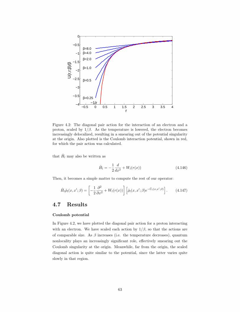
−0.5 0 0.5 1 1.5 2 2.5 3 3.5 4−4

−3.5

−3

−2.5

−2

−1.5

−1

−0.5

0

β=0.25

β=0.5

β=1.0

β=2.0

β=4.0β=8.0

−1/r

r

U(r

,r;β

)/β

PSfrag replacements

Figure 4.2: The diagonal pair action for the interaction of an electron and aproton, scaled by 1/β. As the temperature is lowered, the electron becomesincreasingly delocalized, resulting in a smearing out of the potential singularityat the origin. Also plotted is the Coulomb interaction potential, shown in red,for which the pair action was calculated.

that Hl may also be written as

Hl = −1

2

d

dx2+Wl(r(x)) (4.146)

Then, it becomes a simple matter to compute the rest of our operator:

Hlρl(x, x′;β) =

[

−1

2

∂2

∂x2+Wl(r(x))

] [

ρl(x, x′;β)e−Ul(x,x′;β)

]

. (4.147)

4.7 Results

Coulomb potential

In Figure 4.2, we have plotted the diagonal pair action for a proton interacting

with an electron. We have scaled each action by 1/β, so that the actions are

of comparable size. As β increases (i.e. the temperature decreases), quantum

nonlocality plays an increasingly significant role, effectively smearing out the

Coulomb singularity at the origin. Meanwhile, far from the origin, the scaled

diagonal action is quite similar to the potential, since the latter varies quite

slowly in that region.

63

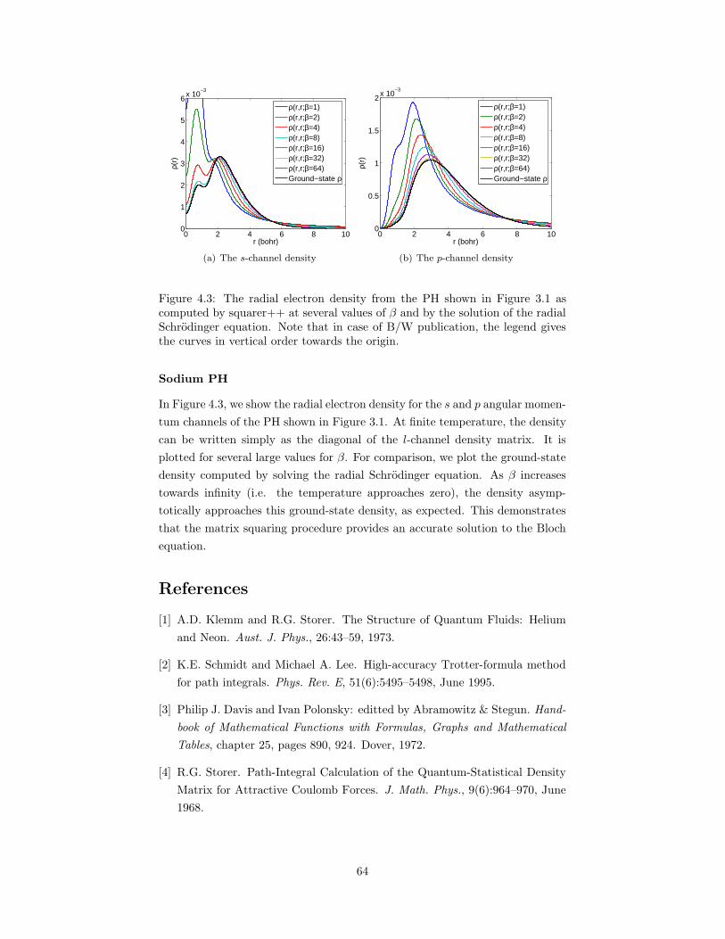
0 2 4 6 8 100

1

2

3

4

5

6x 10

−3

r (bohr)

ρ(r)

ρ(r,r;β=1)ρ(r,r;β=2)ρ(r,r;β=4)ρ(r,r;β=8)ρ(r,r;β=16)ρ(r,r;β=32)ρ(r,r;β=64)Ground−state ρ

(a) The s-channel density

0 2 4 6 8 100

0.5

1

1.5

2x 10

−3

r (bohr)

ρ(r)

ρ(r,r;β=1)ρ(r,r;β=2)ρ(r,r;β=4)ρ(r,r;β=8)ρ(r,r;β=16)ρ(r,r;β=32)ρ(r,r;β=64)Ground−state ρ

(b) The p-channel density

Figure 4.3: The radial electron density from the PH shown in Figure 3.1 ascomputed by squarer++ at several values of β and by the solution of the radialSchrodinger equation. Note that in case of B/W publication, the legend givesthe curves in vertical order towards the origin.

Sodium PH

In Figure 4.3, we show the radial electron density for the s and p angular momen-

tum channels of the PH shown in Figure 3.1. At finite temperature, the density

can be written simply as the diagonal of the l-channel density matrix. It is

plotted for several large values for β. For comparison, we plot the ground-state

density computed by solving the radial Schrodinger equation. As β increases

towards infinity (i.e. the temperature approaches zero), the density asymp-

totically approaches this ground-state density, as expected. This demonstrates

that the matrix squaring procedure provides an accurate solution to the Bloch

equation.

References

[1] A.D. Klemm and R.G. Storer. The Structure of Quantum Fluids: Helium

and Neon. Aust. J. Phys., 26:43–59, 1973.

[2] K.E. Schmidt and Michael A. Lee. High-accuracy Trotter-formula method

for path integrals. Phys. Rev. E, 51(6):5495–5498, June 1995.

[3] Philip J. Davis and Ivan Polonsky: editted by Abramowitz & Stegun. Hand-

book of Mathematical Functions with Formulas, Graphs and Mathematical

Tables, chapter 25, pages 890, 924. Dover, 1972.

[4] R.G. Storer. Path-Integral Calculation of the Quantum-Statistical Density

Matrix for Attractive Coulomb Forces. J. Math. Phys., 9(6):964–970, June

1968.

64

[5] William H. Press, Saul A. Teukolsky, William T. Vetterling, and Brian P.

Flannery. Numerical Recipes in C, chapter 16, pages 710–714. Cambridge

University Press, 1992.

[6] William H. Press, Saul A. Teukolsky, William T. Vetterling, and Brian P.

Flannery. Numerical Recipes in C, chapter 4, page 160. Cambridge Univer-

sity Press, 1992.

65

Chapter 5

Optimized Breakup forLong-Range Potentials

Consider a group of particles interacting with long-ranged central potentials,

vαβ(|rαi − rβ

j |), where the Greek superscripts represent the particle species (e.g.

α = electron, β = proton), and Roman subscripts refer to particle number

within a species. We can then write the total interaction energy for the system

as

V =∑

α

∑

i<j

vαα(|rαi − rα

j |) +∑

β<α

∑

i,j

vαβ(|rαi − r

βj |)

. (5.1)

5.1 The long-range problem

Consider such a system in periodic boundary conditions in a cell defined by

primitive lattice vectors a1, a2, and a3. Let L ≡ n1a1 +n2a2 +n3a3 be a direct

lattice vector. Then the interaction energy per cell for the periodic system is

given by

V =∑

L

∑

α

homologous︷ ︸︸ ︷∑

i<j

vαα(|rαi − rα

j + L|) +

heterologous︷ ︸︸ ︷∑

β<α

∑

i,j

vαβ(|rαi − r

βj + L|)

+∑

L6=0

∑

α

Nαvαα(|L|)︸ ︷︷ ︸

Madelung

,

(5.2)

where Nα is the number of particles of species α. If the potentials vαβ(r) are

indeed long-range, the summation over direct lattice vectors will not converge

in this naive form. A solution to the problem was posited by Ewald. We break

the central potentials into two pieces – a short range part, σ, and a long range

part, Λ, defined by

vαβ(r) = σαβ(r) + Λαβ(r). (5.3)

This is rather unconventional notation, but it alleviates the need to use a sub-

script or superscript. We will perform the summation over images for the short-

range part in real space, while performing the sum for the long-range part in

reciprocal space. For simplicity, we choose σαβ(r) so that it is identically zero at

half the box length and larger, which eliminates the need to sum over multiple

66

images in real space. In this chapter, we develop the details of the method and

provide a way for integrating it into a Path Integral Monte Carlo simulation.

5.2 Reciprocal-space sums

5.2.1 Heterologous terms

We begin with (5.2), starting with the heterologous terms, i.e. the terms in-

volving particles of different species. The short-range terms are trivial, so we

neglect them here. The long-range part is given by

hetero =1

2

∑

α6=β

∑

i,j

∑

L

Λαβ(rαi − r

βj + L). (5.4)

We insert the resolution of unity in real space twice, yielding

hetero =1

2

∑

α6=β

∫

cell

dr dr′∑

i,j

δ(rαi − r)δ(rβ

j − r′)∑

L

Λαβ(|r− r′ + L|) (5.5)

=1

2Ω2

∑

α6=β

∫

cell

dr dr′∑

G,G′,i,j

eiG·(rαi −r)eiG′·(rβ

j −r′)∑

L

Λαβ(|r− r′ + L|)

=1

2Ω2

∑

α6=β

∫

cell

dr dr′∑

G,G′,G′′,i,j

eiG·(rαi −r)eiG′·(rβ

j −r′)eiG′′·(r−r′)ΛαβG′′ ,

where Ω is the volume of the simulation cell. Here, the G summations are over

reciprocal lattice vectors of the supercell given by G = m1b1 +m2b2 +m3b3,

where

b1 = 2πa2 × a3

a1 · (a2 × a3)

b2 = 2πa3 × a1

a1 · (a2 × a3)(5.6)

b3 = 2πa1 × a2

a1 · (a2 × a3).

We note that G · L = 2π(n1m1 + n2m2 + n3m3). The long-range potneitla, Λ,

can be computed in reciprocal space as,

ΛαβG′′ =

1

Ω

∫

cell

dr′′∑

L

e−iG′′·(|r′′+L|)Λαβ(|r′′ + L|), (5.7)

=1

Ω

∫

all space

dr′′ e−iG′′·r′′Λαβ(r′′), (5.8)

67

where Ω is the volume of the cell. Here we have used the fact that the integral

over the cell, summed over all cells, is equivalent to the integral over all space.

hetero =1

2Ω2

∑

α6=β

∫

cell

dr dr′∑

G,G′,G′′,i,j

ei(G·rαi +G′·rβ

j )ei(G′′−G)·re−i(G′′+G′)·r′ΛαβG′′ .

(5.9)

Using the identity,1

Ω

∫

dr ei(G−G′)·r = δG,G′ , (5.10)

we can then perform the integrations over r and r′ to obtain

hetero =1

2

∑

α6=β

∑

G,G′,G′′,i,j

ei(G·rαi +G′·rβ

j )δG,G′′δ−G′,G′′ΛαβG′′ . (5.11)

We now separate the summations, yielding

hetero =1

2

∑

α6=β

∑

G,G′

∑

i

eiG·rαi

︸ ︷︷ ︸

ραG

∑

j

eiG′·rβj

︸ ︷︷ ︸

ρβ

G′

δG,G′′δ−G′,G′′ΛαβG′′ . (5.12)

Here, the ραG coefficients the structure factor, and are not to be confused with

the density matrix. Summing over G and G′, we have

hetero =1

2

∑

α6=β

∑

G′′

ραG′′ ρ

β−G′′Λ

αβG′′ . (5.13)

We can simplify this result a bit further by rearranging the sums over species,

hetero =1

2

∑

α>β

∑

G

(

ραGρ

β−G + ρα

−GρβG

)

ΛαβG (5.14)

=∑

α>β

∑

G

Re(

ραGρ

β−G

)

ΛαβG . (5.15)

5.2.2 Homologous terms

We now consider the terms involving particles of the same species interacting

with each other. The algebra is very similar to that above, with the slight

difficulty of avoiding the self-interaction term:

homologous =∑

α

∑

L

∑

i<j

Λαα(|rαi − rα

j + L|) (5.16)

=1

2

∑

α

∑

L

∑

i6=j

Λαα(|rαi − rα

j + L|) (5.17)

68

Rewriting again in terms of the ρGs, we have

homologous =1

2

∑

α

∑

L

−NαΛαα(|L|) +∑

i,j

Λαα(|rαi − rα

j + L|)

(5.18)

=1

2

∑

α

∑

G

(|ρα

G|2 −Nα)Λαα

G . (5.19)

5.2.3 Madelung terms

Let us now consider the Madelung term for a single particle of species α. This

term corresponds to the interaction of a particle with all of its periodic images.

vαM =

1

2

∑

L6=0

vαα(|L|) (5.20)

=1

2

[

−Λαα(0) +∑

L

Λαα(|L|)]

(5.21)

=1

2

[

−Λαα(0) +∑

G

ΛααG

]

. (5.22)

5.2.4 G = 0 terms

Thus far, we have neglected what happens at the special point G = 0. For many

long-range potentials, such as the Coulomb potential, ΛααG diverges for G = 0.

However, we recognize that for a charge-neutral system, the divergent terms

cancel each other. If all the potentials in the system were precisely Coulomb,

the G = 0 terms would cancel precisely, yielding zero. For systems involving

pseudopotentials, however, it may be the case the resulting term is finite, but

nonzero. Consider the terms from G = 0,

V0 =∑

α>β

NαNβΛαβG=0 +

1

2

∑

α

(Nα)2Λαα

G=0 (5.23)

=1

2

∑

α,β

NαNβΛαβG=0. (5.24)

Next, we must compute ΛαβG=0,

ΛαβG=0 =

4π

Ω

∫ ∞

0

dr r2Λαβ(r). (5.25)

We recognize that this integral will not converge because of the large-r behavior.

However, when we do the sums in (5.24), the large-r parts of the integrals will

cancel precisely. Therefore, we define

ΛαβG=0 ≡

4π

Ω

∫ rend

0

dr r2Λαβ(r), (5.26)

69

where rend is some cutoff value after which the potential tails from the interac-

tions with opposite sign cancel.

5.2.5 Neutralizing background terms

For systems with a net charge, such as the one-component plasma (jellium),

we add a uniform background charge which makes the system neutral. When

we do this, we must add a term to V which comes from the interaction of the

particle with the neutral background. It is a constant term, independent of

the particle positions. In general, we have a compensating background for each

species. These backgrounds will partially cancel out for neutral systems, but not

entirely unless the like-charge potential is precisely opposite the unlike charge

potential (e.g. pure Coulomb). For that reason, the following terms should not

be included in charge-neutral systems. The background contribution can then

be written

Vbackground = −1

2

∑

α

(Nα)2σαα0 −

∑

α>β

NαNβσαβ0 , (5.27)

where σαβ0 is given by

σαβ0 =

4π

Ω

∫ rc

0

r2σ(r) dr, (5.28)

where rc = 12 min(Li) is half the minimum cell dimension.

5.3 Combining terms

Here, we sum all of the terms we computed in the sections above to obtain the

total interaction potential for the system:

V = V0 +∑

α>β

∑

i,j

σ(|rαi − r

βj |) +

∑

G6=0

Re(

ραGρ

β−G

)

ΛαβG −NαNβσαβ

0

+∑

α

NαvαM +

∑

i>j

σ(|rαi − rα

j |) +1

2

∑

G6=0

(|ρα

G|2 −N)Λαα

G −1

2(Nα)

2σαα0

= V0+∑

α>β

∑

i,j

σ(|rαi − r

βj |) +

∑

G6=0

Re(

ραGρ

β−G

)

ΛαβG −NαNβσαβ

0

(5.29)

+∑

α

−NαΛαα(0)

2+∑

i>j

σ(|rαi − rα

j |) +1

2

∑

G6=0

|ραG|2vαα

G − 1

2(Nα)

2σαα0

.

70

5.4 Computing the reciprocal potential

Now we return to (5.8). Without loss of generality, we define for convenience

G = Gz. We may then write the Fourier transform of the potential as

vαβG =

2π

Ω

∫ ∞

0

dr

∫ 1

−1

d(cos θ) r2e−iGr cos(θ)vαβ(r). (5.30)

We do the angular integral first. By inversion symmetry, the imaginary part of

the integral vanishes, yielding

vαβG =

4π

ΩG

∫ ∞

0

dr r sin(Gr)vαβ(r). (5.31)

For the case of the Coulomb potential, the above integral is not formally con-

vergent if we do the integral naively. We may remedy the situation by including

a convergence factor, e−G0r. For a potential of the form vcoul(r) = q1q2/r, this

yields

vscreened coulG =

4πq1q2ΩG

∫ ∞

0

dr sin(Gr)e−G0r (5.32)

=4πq1q2

Ω(G2 +G20). (5.33)

Allowing the convergence factor to tend to zero, we have

vcoulG =

4πq1q2ΩG2

. (5.34)

For more generalized potentials with a Coulomb tail, we cannot evaluate (5.31)

numerically but must handle the Coulomb part analytically. In this case, vαβG

can be written as

vαβG =

4π

Ω

q1q2G2

+

∫ ∞

0

dr r sin(Gr)[

Λαβ(r)− q1q2r

]

. (5.35)

5.5 Efficient calculation methods

5.5.1 Fast computation of ρG

We wish to quickly calculate the quantity

ραG ≡

∑

i

eiG·rαi . (5.36)

71

First, we write

G = m1b1 +m2b2 +m3b3 (5.37)

G · rαi = m1b1 · rα

i +m2b2 · rαi +m3b3 · rα

i (5.38)

eiG·rαi =

[

eib1·rαi

]

︸ ︷︷ ︸

Ciα1

m1[

eib2·rαi

]

︸ ︷︷ ︸

Ciα2

m2[

eib3·rαi

]

︸ ︷︷ ︸

Ciα3

m3

. (5.39)

Now, we note that

[Ciα1 ]m1 = Ciα

1 [Ciα](m1−1). (5.40)

This allows us to recursively build up an array of the C iαs, and then compute

ρG for all G-vectors by looping over all G-vectors, requiring only two complex

multiplies per particle per G. This can save considerable CPU time over the

naive implementation of (5.36). The method is summarized in Algorithm 1.

Algorithm 1 Algorithm to quickly calculate ραG.

Create list of G-vectors and corresponding (m1,m2,m3) indices.for all α ∈ species do

Zero out ραG

for all i ∈ particles do

for j ∈ [1 · · · 3] do

Compute Ciαj ≡ eibj ·rα

i

for m ∈ [−mmax . . .mmax] do

Compute [Ciαj ]m and store in array

end for

end for

for all (m1,m2,m3) ∈ index list do

Compute eiG·rαi = [Ciα

1 ]m1 [Ciα2 ]m2 [Ciα

3 ]m3 from array and add to ραG

end for

end for

end for

5.6 Gaussian charge screening breakup

Ewald’s original approach to the short and long-ranged breakup adds an op-

posite screening charge of gaussian shape around each point charge. It then

removes the charge in the long-ranged part of the potential. For the Coulomb

potential,

Λ(r) =q1q2r

erf(αr), (5.41)

where α is an adjustable parameter used to control how short-ranged the poten-

tial should be. If the box size is L, a typical value for α might be 7/(Lq1q2). We

should note that this form for the long-ranged part of the potential should also

work for any general potential with a Coulomb tail, e.g. pseudo-Hamiltonian

72

potentials. For this form of the long-ranged potential, we have in G-space

vG =4πq1q2 exp

[−G2

4α2

]

ΩG2. (5.42)

5.7 Optimized breakup method

While the choice of Gaussian screening is very simple to implement and nearly

ubiquitous in the simulation community, it is not the most efficient choice for

the breakup. In this section, we undertake the task of choosing the optimal

long-range/short-range partitioning of the potential which minimizes the error

for given real and G-space cutoffs rc and Gc. Here, we modify slightly the

method introduced Natoli and Ceperley [2]. We choose rc = 12 minLi, so that

we require only the nearest image in real space summation. Gc is then chosen

so as to satisfy our accuracy requirements.

Here we modify our notation slightly to accommodate details not required

above. We restrict our discussion to the interaction of two paricles species

(which may be the same), and drop our species indices. Recall from (5.3)

that

v(r) = σ(r) + Λ(r). (5.43)

Define σG and ΛG to be the respective Fourier transforms of the above. The

goal is to choose σ(r) such that its value and first two derivatives vanish at rc,

while making Λ(r) as smooth as possible so that G-space components, ΛG, are

very small for G > Gc. Here, we describe how to do this is an optimal way.

Define the periodic potential, Vp, as

Vp(r) =∑

L

v(|r + L|), (5.44)

where r is the displacement between the two particles and L is a lattice vector.

Let us then define our approximation to this potential, Va, as

Va(r) = σ(r) +∑

|G|<Gc

ΛGeiG·r (5.45)

Now, we seek to minimize the RMS error over the cell,

χ2 =1

Ω

∫

Ω

d3r |Vp(r)− Va(r)|2 (5.46)

We may write

Vp(r) =∑

G

vGeiG·r, (5.47)

where

vG =1

Ω

∫

d3r e−iG·rv(r). (5.48)

73

We now need a basis in which to represent the broken-up potential. We may

choose to represent either σ(r) or Λ(r) in a real-space basis. Natoli and Ceperley

chose the prior in their paper. We choose the latter for a number of reasons.

First, singular potentials are difficult to represent in a linear basis unless the

singularity is explicitly included. This requires a separate basis for each type of

singularity. The short-range potential may have an arbitrary number of features

for r < rc and still be a valid potential. By construction, however, we desire

that Λ(r) be smooth in real-space so that its Fourier transform falls off quickly

with increasing G. We therefore expect that, in general, Λ(r) should be well-

represented by fewer basis functions than σ(r). Finally, the original method

of Natoli and Ceperley required the Fourier transform of the potential. For

potentials with a hard core, this may not be well defined. As we shall see, with

the modified method we introduce here, no information about the potential

inside the core is needed. For all these reasons, we define then

Λ(r) ≡

∑J−1n=0 tnhn(r) for r ≤ rc

v(r) for r > rc.(5.49)

where the hn(r) are a set of J basis functions. We require that the two cases

agree on the value and first two derivatives at rc. We may then define

cnG ≡1

Ω

∫ rc

0

d3r e−iG·rhn(r). (5.50)

Similarly, we define

xG ≡ −1

Ω

∫ ∞

rc

d3r e−iG·rv(r) (5.51)

Therefore,

ΛG = −xG +

J−1∑

n=0

tncnG (5.52)

Because σ(r) goes identically to zero at the box edge, inside the cell it can still

be expanded in a period basis as

σ(r) =∑

G

σGeiG·r. (5.53)

We then write the error in our breakup as

χ2 =1

Ω

∫

Ω

d3r

∣∣∣∣∣∣

∑

G

eiG·r (vG − σG)−∑

|G|≤Gc

eiG·rΛG

∣∣∣∣∣∣

2

. (5.54)

We see that if we define

σ(r) ≡ v(r)− Λ(r), (5.55)

74

then their Fourier transforms must obey the relation,

ΛG + σG = vG. (5.56)

Thus, all terms of the sum in (5.54) for |G| ≤ Gc will cancel. Then we have

χ2 =1

Ω

∫

Ω

d3r

∣∣∣∣∣∣

∑

|G|>Gc

eiG·r (vG − σG)

∣∣∣∣∣∣

2

(5.57)

=1

Ω

∫

Ω

d3r

∣∣∣∣∣∣

∑

|G|>Gc

eiG·rΛG

∣∣∣∣∣∣

2

(5.58)

=1

Ω

∫

Ω

d3r

∣∣∣∣∣∣

∑

|G|>Gc

eiG·r(

−xG +

J−1∑

n=0

tncnG

)∣∣∣∣∣∣

2

. (5.59)

We expand the squared magnitude, obtaining

χ2 =1

Ω

∫

Ω

d3r∑

|G|,|G′|>Gc

ei(G−G′)·r(

xG −J−1∑

n=0

tncnG

)(

xG −J−1∑

m=0

tmcmG′

)

,

(5.60)

and then take the derivative w.r.t. tm, yielding

∂(χ2)

∂tm=

2

Ω

∫

Ω

d3r∑

|G|,|G′|>Gc

ei(G−G′)·r(

xG −J−1∑

n=0

tncnG

)

cmG′ . (5.61)

We integrate w.r.t. r, yielding a Kronecker δ,

∂(χ2)

∂tm= 2

∑

|G|,|G′|>Gc

δG,G′

(

xG −J−1∑

n=0

tncnG

)

cmG′ . (5.62)

Summing over G′ and equating the derivative to zero, we find the minimum of

our error function is given by

J−1∑

n=0

∑

|G|>Gc

cmGcnGtn =∑

|G|>Gc

xGcmG, (5.63)

which is equivalent in form to equation (19) in [2], where we have xG, instead of

vG. Thus, we see that we may optimize the short-range or long-range potential

simply by choosing to use vG or xG in the above equation. We now define

Amn ≡∑

|G|>Gc

cmGcnG (5.64)

bm ≡∑

|G|>Gc

xGcmG. (5.65)

Thus, it becomes clear that our minimization equations can be cast in the

75

canonical linear form,

At = b. (5.66)

5.7.1 Solution by SVD

In practice, we note that the matrix A frequently becomes nearly singular in

practice, and using a standard matrix inversion to solve (5.66) would be unsta-

ble. For this reason, we use the singular value decomposition to solve for tn.

This factorization decomposes A as

A = USVT , (5.67)

where UT U = VT V = 1 and S is diagonal. In this form, we have

t =

J−1∑

i=0

(U(i) · b

Sii

)

V(i), (5.68)

where the parenthesized subscripts refer to columns. The advantage of this form

is that the singular values, Sii, can be used to detect and eliminate singular be-

havior. In particular, if Sii is zero or very near zero, the contribution of the ith

column of V may be neglected in the sum in (5.68), since it represents a nu-

merical instability and has little physical meaning. Small singular values reflect

the fact that the system cannot distinguish between two linear combinations of

the basis functions. Using the SVD in this manner is guaranteed to be stable.

This decomposition is available in LAPACK in the DGESVD subroutine.

5.7.2 Constraining values

Often, we wish to constrain the value of tn to have a fixed value to enforce a

boundary condition, for example. To do this, we define

b′ ≡ b− tnA(n). (5.69)

We then define A∗ as A with the nth row and column removed, and b∗ as b′ with

the nth element removed. Then we solve the reduced equation A∗t∗ = b∗, and

finally insert tn back into the appropriate place in t∗ to recover the complete,

constrained vector t. This approach may be trivially generalized to an arbitrary

number of constraints.

5.7.3 The LPQHI basis

The above discussion was general and independent of the basis used to represent

Λ(r). In this section, we introduce a convenient basis of localized piecewise-

quintic Hermite interpolant (LPQHI) functions, similar to those used for splines,

which have a number of useful properties. This basis was first used in [2].

76

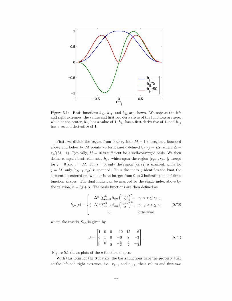
−1 −0.5 0 0.5 1

−1

−0.5

0

0.5

1

r−rj

hj0

hj1

*5h

j2*50

Figure 5.1: Basis functions hj0, hj1, and hj2 are shown. We note at the leftand right extremes, the values and first two derivatives of the functions are zero,while at the center, hj0 has a value of 1, hj1 has a first derivative of 1, and hj2

has a second derivative of 1.

First, we divide the region from 0 to rc into M − 1 subregions, bounded

above and below by M points we term knots, defined by rj ≡ j∆, where ∆ ≡rc/(M − 1). Typically, M = 10 is sufficient for a well-converged basis. We then

define compact basis elements, hjα which span the region [rj−1, rj+1], except

for j = 0 and j = M . For j = 0, only the region [r0, r1] is spanned, while for

j = M , only [rM−1, rM ] is spanned. Thus the index j identifies the knot the

element is centered on, while α is an integer from 0 to 2 indicating one of three

function shapes. The dual index can be mapped to the single index above by

the relation, n = 3j + α. The basis functions are then defined as

hjα(r) =

∆α∑5

n=0 Sαn

(r−rj

∆

)n

, rj < r ≤ rj+1

(−∆)α∑5

n=0 Sαn

(rj−r

∆

)n

, rj−1 < r ≤ rj0, otherwise,

(5.70)

where the matrix Sαn is given by

S =

1 0 0 −10 15 −6

0 1 0 −6 8 −3

0 0 12 − 3

232 − 1

2

. (5.71)

Figure 5.1 shows plots of these function shapes.

With this form for the S matrix, the basis functions have the property that

at the left and right extremes, i.e. rj−1 and rj+1, their values and first two

77

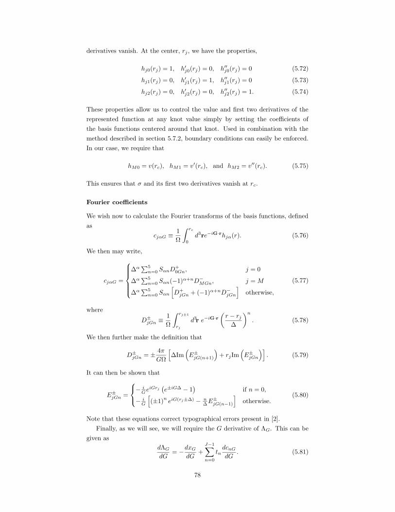
derivatives vanish. At the center, rj , we have the properties,

hj0(rj) = 1, h′j0(rj) = 0, h′′j0(rj) = 0 (5.72)

hj1(rj) = 0, h′j1(rj) = 1, h′′j1(rj) = 0 (5.73)

hj2(rj) = 0, h′j2(rj) = 0, h′′j2(rj) = 1. (5.74)

These properties allow us to control the value and first two derivatives of the

represented function at any knot value simply by setting the coefficients of

the basis functions centered around that knot. Used in combination with the

method described in section 5.7.2, boundary conditions can easily be enforced.

In our case, we require that

hM0 = v(rc), hM1 = v′(rc), and hM2 = v′′(rc). (5.75)

This ensures that σ and its first two derivatives vanish at rc.

Fourier coefficients

We wish now to calculate the Fourier transforms of the basis functions, defined

as

cjαG ≡1

Ω

∫ rc

0

d3re−iG·rhjα(r). (5.76)

We then may write,

cjαG =

∆α∑5

n=0 SαnD+0Gn, j = 0

∆α∑5

n=0 Sαn(−1)α+nD−MGn, j = M

∆α∑5

n=0 Sαn

[

D+jGn + (−1)α+nD−

jGn

]

otherwise,

(5.77)

where

D±jGn ≡

1

Ω

∫ rj±1

rj

d3r e−iG·r(r − rj

∆

)n

. (5.78)

We then further make the definition that

D±jGn = ± 4π

GΩ

[

∆Im(

E±jG(n+1)

)

+ rjIm(

E±jGn

)]

. (5.79)

It can then be shown that

E±jGn =

− iGe

iGrj(e±iG∆ − 1

)if n = 0,

− iG

[

(±1)neiG(rj±∆) − n

∆E±jG(n−1)

]

otherwise.(5.80)

Note that these equations correct typographical errors present in [2].

Finally, as we will see, we will require the G derivative of ΛG. This can be

given as

dΛG

dG= −dxG

dG+

J−1∑

n=0

tndcnG

dG. (5.81)

78

Hence, we must compute

dcnG

dG=

∆α∑5

n=0 SαnD+0Gn, j = 0

∆α∑5

n=0 Sαn(−1)α+nD−MGn, j = M

∆α∑5

n=0 Sαn

[

D+jGn + (−1)α+nD−

jGn

]

otherwise,

(5.82)

where the dots represent differentiation w.r.t. G.

D±jGn = −

D±jGn

G± 4π

GΩ

[

∆Im(

E±jG(n+1)

)

+ rjIm(

E±jGn

)]

. (5.83)

Finally,

E±jGn =

− iGe

iGrj(e±iG∆ − 1

)if n = 0,

− iG

[

(±1)neiG(rj±∆) − n

∆ E±jG(n−1)

]

otherwise.(5.84)

5.7.4 Enumerating G-points

We note that the summations over G which have been ubiquitous in this chapter

requires enumeration of the G-vectors. In particular, we should sum over all

|G| > Gc. In practice, we must limit our summation to some finite cutoff

value Gc < |G| < Gmax. A value Gmax of order 3000/Lmin gives very good

convergence, where Lmin is the minimum box dimension. Enumerating these

vectors in a naive fashion even for this finite cutoff would prove quite prohibitive,

as it requires ∼ 109 vectors.

Our first optimization comes in realizing that all quantities in this calculation

require only the scalar magnitude, |G|, and not G itself. Thus, we may take

advantage of the great degeneracy of |G|. We create a list of (G,N) pairs, where

N is the number of vectors with magnitude G. We make nested loops over n1,

n2, and n3, yielding the vector G = n1b1 +n2b2 +n3b3 for each integer triplet.

If |G| is in the required range, we check to see if there is already an entry with

that magnitude on our list, incrementing the corresponding N if there is, or

creating a new entry if not. Doing so typically saves a factor of ∼ 200 in storage

and computation.

This reduction is still not sufficient for large Gmax, since it requires that

we still loop through over 109 entries. To further reduce cost, we may pick

an intermediate cutoff, Gcont, above which we will approximate the degeneracy

assuming a continuum of G-points. We stop our exact enumeration at Gcont,

and then add ∼ 1000 points, Gi, uniformly spaced between Gcont and Gmax.

We then approximate the degeneracy by

Ni =4π3

(G3

b −G3a

)

(2π)3/Ω, (5.85)

where Gb = (Gi+Gi+1)/2 and Ga = (Gi+Gi−1)/2. The numerator on the RHS

79

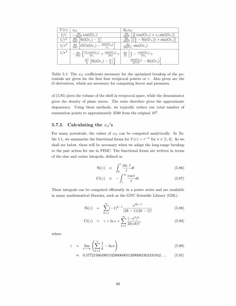
V (r) xG ∂GxG

1/r − 4πΩG2 cos(Grc)

4πΩG2

[2G cos(Grc) + rc sin(Grc)

]

1/r2 4πΩG

[Si(Grc)− π

2

]4π

ΩG2

[(π2 − Si(Grc)

)+ sin(Grc)

]

1/r3 4πΩG

[

GCi(Grc)− sin(Grc)rc

]4π

ΩG2rcsin(Grc)

1/r4 − 4πΩG

G cos(Grc)

2rc+ sin(Grc)

2r2c

+

G2

2

[Si(Grc)− π

2

]

2πΩ

[π2 −

cos(Grc)Grc

+

sin(Grc)G2r2

c− Si(Grc)

]

Table 5.1: The xG coefficients necessary for the optimized breakup of the po-tentials are given for the first four reciprocal powers or r. Also given are theG-derivatives, which are necessary for computing forces and pressures.

of (5.85) gives the volume of the shell in reciprocal space, while the denominator

gives the density of plane waves. The ratio therefore gives the approximate

degeneracy. Using these methods, we typically reduce our total number of

summation points to approximately 2500 from the original 109.

5.7.5 Calculating the xG’s

For many potentials, the values of xG can be computed analytically. In Ta-

ble 5.1, we summarize the functional forms for V (r) = r−n for n ∈ [1, 4]. As we

shall see below, these will be necessary when we adapt the long-range breakup

to the pair action for use in PIMC. The functional forms are written in terms

of the sine and cosine integrals, defined as

Si(z) ≡∫ z

0

sin t

tdt (5.86)

Ci(z) ≡ −∫ ∞

z

cos t

tdt. (5.87)

These integrals can be computed efficiently in a power series and are available

in many mathematical libraries, such as the GNU Scientific Library (GSL).

Si(z) =

∞∑

k=1

(−1)k−1 x2k−1

(2k − 1)(2k − 1)!(5.88)

Ci(z) = γ + ln z +

∞∑

k=1

(−x2)k

2k(sk)!, (5.89)

where

γ = limn→∞

(n∑

k=1

1

k− lnn

)

(5.90)

≈ 0.577215664901532860606512090082402431042 . . . (5.91)

80

PSfrag replacements

V (r)

V(r

)

Vl(r)Vs(r)

r (bohr)

(a) Optimized breakup of a 1/r potential.

PSfrag replacements

U(r)

U(r

)

Ul(r)Us(r)

r (bohr)

(b) Optimized breakup of a pair action.

Figure 5.2: Two example results of the optimized breakup method.

! "$#%&' ( !)' *!+-,/.0. "' .1243 * 56%&) 87

PSfrag replacements

Gcrc

ln(Lχ)

Figure 5.3: The average error in the short-range/long range breakup of theCoulomb potential.

5.7.6 Results for the Coulomb potential

Figure 5.2(a) shows the result of an optimized breakup applied to the Coulomb

potential. In this case, the box size was (25.8 bohr)3 and Gc = 1.2 bohr−1.

As can be seen from the plot, the long range part is extremely smooth and the

short-range part decays very rapidly to zero by r = L2 = 12.9 bohr.

Figure 5.3 shows the error incurred by truncating our reciprocal-space sum

at a finite Gc. On the horizontal axis is plotted the product, Gcrc. This dimen-

sionless number can be related approximately to the number of discrete shells

that are included in the reciprocal-space sum. As is clearly seen, the error de-

cays exponentially with Gc and rc, at a much higher rate than the standard

Ewald method. This implies that substantially higher accuracy can be achieved

with the same number of G-vectors. Alternatively, we can reduce the CPU time

81

while retaining the same accuracy as the Ewald method by reducing the number

of G-vectors.

Also plotted in Figure 5.3 is the original work of Natoli and Ceperley [2].

We note that the modified method of this work has the same convergence prop-

erties as the original optimization method. Note also that the step-like drop at

particular values of Gcrc is the result of an additional shell in reciprocal space.

5.8 Adapting to PIMC

5.8.1 Pair actions

Let us begin by summarizing what we have done so far. We began with the

many-body Hamiltonian given by

H =∑

i

−λi∇2i + V, (5.92)

where V is the periodic potential given by (5.1), and λi ≡ ~2

2mi.

In Chapter 4, we approximately solved for the action of this Hamiltonian

by taking the particles pairwise, and solving for the density matrix of each pair

exactly using the matrix squaring method. This yields the pair action, defined

by

ραβ(r, r′; τ) ≡ ρ0(r, r′; τ)e−uαβ(r,r′;τ), (5.93)

where ρ0 is the free particle density matrix for species α interacting with species

β. ραβ is the density matrix for the pair Hamiltonian

Hαβ = −λαβ∇2 + vαβ(|r|), (5.94)

where r ≡ ri− rj and particles i and j are members of species α and β, respec-

tively, and λαβ is given by

λαβ =~

2

2mα+

~2

2mβ. (5.95)

If the potential vαβ(r) is long range, then the action, uαβ(r, r′; τ), will also be

long range. We note, however, that the action is not a simple function of the

scalar r, as the potential is. At large distances, the action is well-approximated

by

uαβ(r, r′; τ) ≈ 1

2

[uαβ(r, r; τ) + uαβ(r′, r′; τ)

](5.96)

=1

2

[

uαβdiag(r, τ) + uαβ

diag(r′, τ)

]

(5.97)

This is known as the diagonal approximation. Thus, as long as this approxima-

tion is valid at half the minimum box dimension, we may break up the diagonal

82

action as we did the potential. This effectively neglects the off-diagonal parts

of the action for particles more than a half-box length apart, but experience

has shown that these contributions are usually quite small. The same analysis

follows for the τ -derivative of the action, uαβ(r, r′; τ), which is required to com-

pute the total energy. Note that PIMC simulation requires the pair action at

several values of τ , so that in practice, we need to do several optimized breakups

for each uαβdiag and uαβ

diag and a single breakup for each potential interaction, vαβ .

5.8.2 Results for a pair action

Figure 5.2(b) shows an example of the optimized breakup of the diagonal pair ac-

tion for an electron interacting with a sodium atom. The form of the long range

action, u(r), is extremely similar to the long range potential in Figure 5.2(a).

This reflects the advantage of the modified method presented here that the form

of the potential (action) for r < rc has no bearing on the form of the long range

potential (action). Since both the Coulomb potential and pseudo pair action

have Coulomb tails, the resulting breakups have extremely similar long-range

parts (neglecting the sign, of course).

5.9 Beyond the pair approximation: RPA

improvements

Consider the limit of a dense gas of charged particles. We know from solid

state theory that collective density fluctuations, known as plasmons, contribute

significantly to the energy spectrum of such a system. An approximation to

the density matrix determined by considering only pairs of particles will neglect

these contributions at finite τ . As τ approaches zero, the Trotter theorem still

guarantees we will approach the right limit.

Nonetheless, it is possible to significantly reduce the finite-τ timestep error

by utilizing a different approximation for the long range part of the action. In

this section, we develop a formalism based on a random phase approximation

solution to the Bloch equation. This approach was first developed in the context

of variational Monte Carlo by Ceperley [1]. It was later generalized to actions

by Pollock and Ceperley and was first published in the dissertation of William

Magro [4]. We have attempted to be more explicit in the derivation here than

in previous publications.

We begin by defining our effective, long-range potential. As noted above, we

may perform an optimized breakup on the diagonal action, uαβdiag(r).

uαβdiag(r) = uαβ

diag(r) + uαβdiag(r), (5.98)

where the u and u refer to the short and long range diagonal actions, respectively,

borrowing the notation for short and long vowels. We subtract the long range

83

part from the total pair action in a quasi-primitive approximation by defining

uαβdiag(r) ≡ τ vαβ(r). (5.99)

Let vαβG represent the Fourier transform of the effective potential, vαβ(r). Fi-

nally, let its short-range counterpart be defined by

vαβG ≡ vαβ

G − vαβG . (5.100)

Now, we wish to reintroduce a new long range action, which we will calculate

in G-space within the Random Phase Approximation (RPA). We begin with the

Bloch equation,

ρ = −Hρ, (5.101)

where the dot refers to differentiation w.r.t. τ . The Hamiltonian is given by

H =

[

−∑

α

∑

i∈α

λα∇2i

]

+ V + V , (5.102)

where V and V are the total short and long range periodic potentials, respec-

tively. Let us now make the partitioning that

ρ(R,R′; τ) = ρ0(R,R′; τ)e−U(R,R′;τ)e−U(R,R′;τ). (5.103)

At the moment, this is purely definitional. Our task in this section will be to

find U and U such that the density matrix in (5.103) approximately satisfies

the Bloch equation.

We assume that ρs ≡ ρ0e−U satisfies the Bloch equation for the short-range

Hamiltonian,

Hs =

[

−∑

α

∑

i∈α

λα∇2i

]

+ V . (5.104)

In fact, this is only strictly true in the limit of τ → 0, but this approximation

will suffice for our present analysis. Recalling the vector identity ∇2(ab) =

a∇2b+ b∇2a+ 2(∇a) · (∇b), we have for our Bloch equation,

−[

ρs − ρs˙U]

e−U =∑

α, i∈α

−λα

[

ρs∇2i e

−U + e−U∇2i ρs + 2(∇iρs) · (∇ie

−U )]

+(V + V )ρse−U . (5.105)

Subtracting the Bloch equation for the short range part, we are left with

[˙U − V

]

ρse−U =

∑

α, i∈α

−λα

[

ρs∇2i e

−U + 2(∇iρs) · (∇ie−U )

]

. (5.106)

84

Recall that

∇e−U = −∇Ue−U (5.107)

∇ρ0 = 0 (for R = R′) (5.108)

∇ρs = −ρs∇U (5.109)

∇2e−U =[(∇U)2 −∇2U

]e−U . (5.110)

We now attempt to solve the Bloch equation under the restriction that R = R′,

i.e. along the diagonal of the density matrix. Hence let us define

U(R,R′; τ) ≡ 1

2

[U(R; τ) + U(R′; τ)

](5.111)

U(R,R′; τ) ≡ 1

2

[

U(R; τ) + U(R′; τ)]

(5.112)

as the long and short range diagonal actions written as functions of only one

spatial argument. Then we have, along the diagonal,

∇U =1

2∇U (5.113)

∇2U =1

2∇2U . (5.114)

Substituting back into our Bloch equation we obtain

˙U =∑

α, i∈α

−λα

1

4(∇iU)2 − 1

2∇2

i U +1

2(∇iU) · (∇iU)

+ V (5.115)

We recall that the long range potential, V , may be written as

V =1

2

∑

G

∑

α,β

ραGρ

β−GΛαβ

G . (5.116)

We may similarly write U and U in terms of uαβG and uαβ

G .

We now proceed to calculate gradients and laplacians. Recalling that

ραG =

∑

i∈α

eiG·ri , (5.117)

85

we write,

∇iU =1

2

∑

G

[

iGeiG·ri

∑

α

ρα−Gu

αβG + c.c.

]

(5.118)

=1

2

∑

G

2Re[

iGeiG·ri

∑

α

ρα−Gu

αβG

]

(5.119)

= Re[∑

G

iGeiG·ri

∑

α

ρα−Gu

αβG

]

(5.120)

=∑

G

iGeiG·ri

∑

α

ρα−Gu

αβG . (5.121)

Next, we compute the Laplacian w.r.t. the ith particle.

∇2iU = ∇i · ∇iU (5.122)

= ∇i ·∑

G

iGeiG·ri

∑

α

ρα−Gu

απi

G (5.123)

=∑

G

iG · ∇i

[

eiG·ri

∑

α

ρα−Gu

απi

G

]

(5.124)

=∑

G

G2

[

uπiπi

G − eiG·ri

∑

α

ρ−Guαπi

G

]

, (5.125)

where πi is the species of the ith particle. Now, let us sum over all particles,

∑

i

λi∇2iU =

∑

G

G2

∑

β

NβuββG − ρ

βG

∑

α

ρ−GuαβG

(5.126)

=∑

G

G2∑

α,β

λβ

[

Nαδα,β − ρα−Gρ

βG

]

uαβG . (5.127)

Now, let us consider the cross term,

(∇iU) · (∇iU) =

[∑

G

iGeiG·ri

∑

α

ρα−Gu

πiαG

]

·

∑

q

iqeiq·ri

∑

β

ρβ−Gu

πiβG

= −∑

G,q

G · qei(G+q)·ri

∑

α,β

ρα−Gρ

β−qu

απi

G uβπi

G . (5.128)

Again, summing over all particles, we have

∑

i

(∇iU) · (∇iU) = −∑

G,q

G · q∑

α,β,γ

ργG+qρ

α−Gρ

β−qu

αγG uβγ

G . (5.129)

Similarly,

∑

i

(∇iU)2 = −∑

G,q

G · q∑

α,β,γ

ργG+qρ

α−Gρ

γ−qu

αγG uβγ

G . (5.130)

86

Using the random phase approximation (RPA) amounts to the assumption

that ργG+q ≈ NγδG,−q. Making this substitution, we have

∑

i

(∇iU) · (∇iU)RPA≈

∑

G

G2∑

α,β,γ

Nγρα−Gρ

βGu

αγG uβγ

G (5.131)

∑

i

(∇iU)2RPA≈

∑

G

G2∑

α,β,γ

Nγρα−Gρ

βGu

αγG uβγ

G . (5.132)

We now return to the Bloch equation,

∑

G

∑

α,β

1

2ραGρ

β−G

(

˙uG − vαβG

)

+1

2λαG

2uαβG

(

ρα−Gρ

βG −Nβδα,β

)

−∑

γ

G2Nγλγρα−Gρ

βG

[1

4uαγ

G uβγG +

1

2uαγ

G uβγ

]

= 0,

(5.133)

and symmetrize this equation w.r.t. α and β to obtain

∑

G,α,β

(

ραGρ

β−G + ρα

−GρβG

)[

˙uαβG − Λαβ

G +G2

(λα + λβ

2

)

uαβG

+∑

γ

G2

2Nγ

(

uαγG uβγ

G + uαγG uβγ

G + uαγG uβγ

G

)]

−G2Nαδαβ

= 0.

(5.134)

We require that this expression hold independent of the positions of the particles,

i.e. independent of the values of ραG and ρβ

G. Thus, the equations separate for

each value of G, α, and β. In particular, for G 6= 0,

˙uαβG = Λαβ

G −G2

(λα + λβ

2

)

uαβG −

G2

2

∑

γ

Nγ

(

uαγG uβγ

G + uαγG uβγ

G + uαγG uβγ

G

)

.

(5.135)

Next, we need an equation for the imaginary time propagation of uαβG . Above,

we assumed that u was the solution to the short-range problem. Our Bloch

equation for U is then given by

˙U =∑

i

−λi

1

4(∇iU −

1

2∇2

i U

+ V . (5.136)

Following the RPA procedure above, we arrive at the following equation for each

uαβG .

˙uαβG = vαβ

G −G2

(λα + λβ

2

)

uαβG −

G2

2

∑

γ

Nγ uαγG uβγ

G . (5.137)

Hence, for each value of G, we have a coupled set of differential equations we

must solve. We note that while the equations for u couple to u, those for u do

not couple to u. These equations do not couple different values of G, but they

do couple all the species together. Therefore, if we have Nsp species, for each

87

value of G we have Nsp(Nsp + 1) coupled first-order differential equations. The

coupled systems can be solved individually with an ODE integrator such as the

Runge Kutta method [3] with the initial conditions that

uαβG (τ = 0) = 0 (5.138)

uαβG (τ = 0) = 0. (5.139)

The system must be integrated from 0 to τ for each value of τ to be used in

the simulation. The equations need only be solved once at the beginning of the

simulation and then tabulated. Doing so will generally reduce the time-step

error.

5.10 Summary

In this chapter, we have introduced the problems associated with simulating

periodic systems containing long-range potentials. We first laid out the classic

solution of Ewald. We then introduced the optimized breakup method of Na-

toli and Ceperley, and suggested a modification to the method that improves

robustness and the range of applicability to potentials with singularities inside

the real-space cutoff, rc. We showed that this optimized method gives results

much more accurate that the original Ewald method with the same CPU time.

We then suggested how this method could be implemented in a PIMC simula-

tion containing pseudohamiltonians by breaking up the diagonal part of the pair

action. Finally, we showed how the time step error could be reduced through a

solution of the Bloch equation within the random phase approximation, follow-

ing the work first published in [4].

References

[1] D. Ceperley. Ground state of the fermion one-component plasma: A Monte

Carlo study in two and three dimensions. Phys. Rev. B, 18(7):3126–3138, 1

October 1978.

[2] Vincent Natoli and David M. Ceperley. An Optimized Method for Treating

Long-Range Potentials. Journal of Computational Physics, 117:171–178,

1995.

[3] William H. Press, Saul A. Teukolsky, William T. Vetterling, and Brian P.

Flannery. Numerical Recipes in C, chapter 16, pages 710–714. Cambridge

University Press, 1992.

[4] William R. Magro. Quantum Monte Carlo studies of dense hydrogen and

two-dimensional Bose liquids. PhD thesis, University of Illinois at Urbana-

Champaign, 1994.

88

Chapter 6

Twist-averaged boundaryconditions

6.1 Bulk properties

In condensed matter physics, it is rare that one simulates a system of, say,

sixteen particles because one is interested in the properties of the sixteen-particle

system. Rather, one is most often interested in the bulk properties of a system,

i.e. the per-particle properties in the thermodynamic limit. For obvious reasons,

simulation of a system of O(1023) particles is impossible. One usually simulates

the largest system that can be handled practically, with the hope that the finite

system properties will approximately match the infinite system limit.

As mentioned in Chapter 2, the use of periodic boundary conditions (PBC)

greatly improves the convergence of properties calculated in finite simulations

to the bulk limit by eliminating surface effects. In quantum Monte Carlo, PBC

implies that the many-body wave function has the same value if a particle is

translated by a multiple of a lattice vector of the simulation cell. Unfortu-

nately, in the case of metallic systems the use of PBC still leads to rather slow

convergence, since the Fermi surface is quite poorly represented.

In 2001, Lin, Zong, and Ceperley introduced twist-averaged boundary con-

ditions (TABC) to reduce these errors in ground-state QMC simulations [1]. In

this method, when a particle is translated by a box length, the wave function

picks up a phase, θ, which is called the twist. Specifically,

Ψ(r1 + Lxx, r2, . . . ) = eiθxΨ(r1, r2 . . . ). (6.1)

In three dimensions, there is a separate twist for each axis of the simulation

cell, i.e. θ = (θx, θy, θz). In general, each twist angle is restricted to the interval

−π < θi ≤ π, but in the case of a real potential the range of one of the three

angles may be further restricted to 0 < θx ≤ π because of time-reversal sym-

metry. Following the approach used in solid state physics, we can decompose Ψ

into a periodic part, Ψk and a twist part, or

Ψθ(ri) = exp

[

ik ·∑

i

ri

]

Ψk(ri), (6.2)

89

where k is given by

k =

(θx

Lx,θy

Ly,θz

Lz

)

(6.3)

for a simulation cell of dimensions Lx × Ly × Lz.

Given this definition for twisted boundary conditions, we can then compute

twist-averaged properties by integrating over the twist vector. For an observable

operator O in a 3D system with a real potential, we write its expectation value

as⟨

O⟩

TABC=

1

4π3

∫

dθ⟨

Ψθ

∣∣∣O∣∣∣Ψθ

⟩

, (6.4)

where the integration is over 0 to π for θx and −π to π for θy and θz. The

twist averaging mitigates many of the finite-size errors arising from the kinetic

energy, so that, in general, 〈O〉TABC will be much closer to the bulk limit than

〈O〉PBC. To see why this is the case, we introduce a simple example in the next

section.

6.2 Example: free fermions in 2D

As an illustrative example, let us consider a 2D periodic system containing spin-

less free fermions. The single-particle eigenstates for the system are naturally

plane waves, which can be labeled by a band index, i, and a crystal momentum,

k (or the equivalent twist vector). These eigenstates can be written

ψik(r) = ei(Gi+k)·r, (6.5)

where

Gi =

(2πnx

Lx,2πny

Ly

)

, (6.6)

and nx and ny are integers. For an N -particle system with a given twist k, the

N plane waves with lowest energy Eik = 12 |Gi + k|2 will be occupied.

Figure 6.1 shows a diagram of the reciprocal space occupation for two such

systems with the same particle density, ρ = N/(LxLy). Figure 6.1(a) shows a

plot for a system of N = 13 particles in a square box of sides Lx = Ly = 2π.

Figure 6.1(b) gives the same plot for N = 52 particles and Lx = Ly = 4π. In

both cases, since there is no potential, the system will have a circular Fermi

surface with radius kf = 2(πρ)12 ≈ 2.034. This surface is denoted by the large

black circle in each plot.

Periodic boundary conditions

Consider first the 13-particle system shown in Figure 6.1(a). In an ideal sim-

ulation which would yield the exact bulk energy, all plane waves in reciprocal

space for which |G + k| < kf should be occupied and those with higher en-

ergy unoccupied. Most current QMC simulations are performed with periodic

90

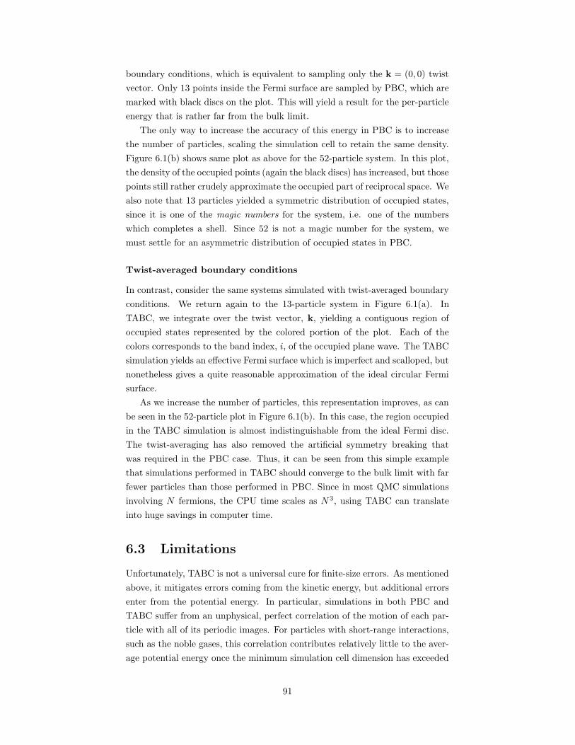
boundary conditions, which is equivalent to sampling only the k = (0, 0) twist

vector. Only 13 points inside the Fermi surface are sampled by PBC, which are

marked with black discs on the plot. This will yield a result for the per-particle

energy that is rather far from the bulk limit.

The only way to increase the accuracy of this energy in PBC is to increase

the number of particles, scaling the simulation cell to retain the same density.

Figure 6.1(b) shows same plot as above for the 52-particle system. In this plot,

the density of the occupied points (again the black discs) has increased, but those

points still rather crudely approximate the occupied part of reciprocal space. We

also note that 13 particles yielded a symmetric distribution of occupied states,

since it is one of the magic numbers for the system, i.e. one of the numbers

which completes a shell. Since 52 is not a magic number for the system, we

must settle for an asymmetric distribution of occupied states in PBC.

Twist-averaged boundary conditions

In contrast, consider the same systems simulated with twist-averaged boundary

conditions. We return again to the 13-particle system in Figure 6.1(a). In

TABC, we integrate over the twist vector, k, yielding a contiguous region of

occupied states represented by the colored portion of the plot. Each of the

colors corresponds to the band index, i, of the occupied plane wave. The TABC

simulation yields an effective Fermi surface which is imperfect and scalloped, but

nonetheless gives a quite reasonable approximation of the ideal circular Fermi

surface.

As we increase the number of particles, this representation improves, as can

be seen in the 52-particle plot in Figure 6.1(b). In this case, the region occupied

in the TABC simulation is almost indistinguishable from the ideal Fermi disc.

The twist-averaging has also removed the artificial symmetry breaking that

was required in the PBC case. Thus, it can be seen from this simple example

that simulations performed in TABC should converge to the bulk limit with far

fewer particles than those performed in PBC. Since in most QMC simulations

involving N fermions, the CPU time scales as N 3, using TABC can translate

into huge savings in computer time.

6.3 Limitations

Unfortunately, TABC is not a universal cure for finite-size errors. As mentioned

above, it mitigates errors coming from the kinetic energy, but additional errors

enter from the potential energy. In particular, simulations in both PBC and

TABC suffer from an unphysical, perfect correlation of the motion of each par-

ticle with all of its periodic images. For particles with short-range interactions,

such as the noble gases, this correlation contributes relatively little to the aver-

age potential energy once the minimum simulation cell dimension has exceeded

91

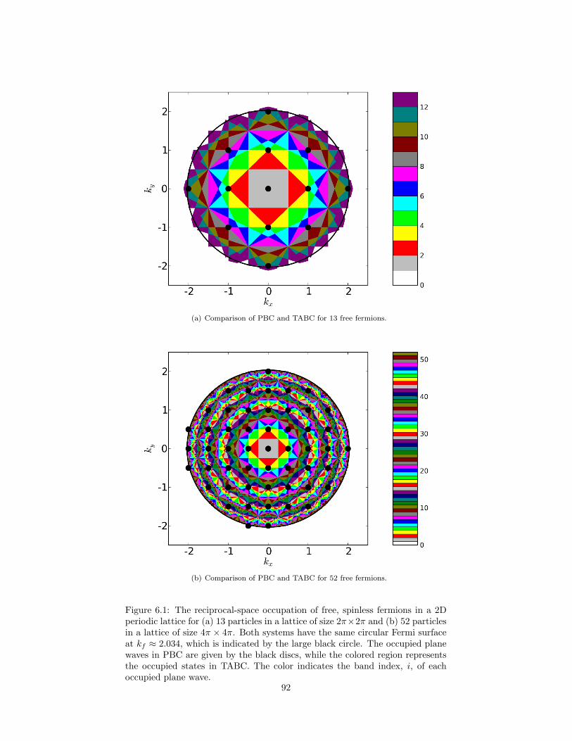
(a) Comparison of PBC and TABC for 13 free fermions.

(b) Comparison of PBC and TABC for 52 free fermions.

Figure 6.1: The reciprocal-space occupation of free, spinless fermions in a 2Dperiodic lattice for (a) 13 particles in a lattice of size 2π×2π and (b) 52 particlesin a lattice of size 4π × 4π. Both systems have the same circular Fermi surfaceat kf ≈ 2.034, which is indicated by the large black circle. The occupied planewaves in PBC are given by the black discs, while the colored region representsthe occupied states in TABC. The color indicates the band index, i, of eachoccupied plane wave.

92

the range of the potential. For systems containing long-range Coulomb inter-

actions, however, the finite size errors in the potential energy are much more

severe.

There are at least two partial solutions to this problem. First, the simulation

can be performed with several values for the number of particles, N , while

maintaining constant density. The average value of the potential energy, 〈V 〉may then be plotted versus N , and the resulting curve extrapolated to N →∞.

While TABC does not, in general, reduce the magnitude of the potential energy

error, it does make this 〈V 〉 versus N curve much smoother, making the said

extrapolation much easier.

As an alternative approach, the potential energy errors can be corrected

a posteriori through a method developed by Chiesa, Ceperley, Martin, and

Holzmann [3]. In this method, it is recognized that the majority of the error

comes from the long-wavelength components of the structure factor, SG. In

particular, a finite-size simulation with cell size L omits the contribution to the

potential energy from all wave vectors smaller than 2π/L. By fitting SG to an

analytic function for small |G|, the missing contribution can be recovered. The

details of this method are beyond the scope of this work.

6.4 Implementation in PIMC

Thus far in this chapter, we have discussed TABC in the generic context of

QMC simulations and wave functions. In this section, we discuss how TABC

may be incorporated into a PIMC simulation involving density matrices. In

our previous discussion of PIMC, we have assumed that the density matrix,

ρ(R,R′;β) is a purely real quantity. In order to perform twist averaging, we

must allow the density matrix to become complex. As we shall see in the

following chapter, we break the complex density matrix into two pieces – a real

magnitude and a complex phase. While it is theoretically possible to formulate a

PIMC simulation in which both the magnitude and phase are solved for exactly,

doing so would result in a fermion phase problem in exact analogy with the

fermion sign problem discussed in Chapter 2. This problem is approximately

solved through the fixed-phase approximation, which will be detailed in the next

chapter. For the moment, it is sufficient to say that this approximation adds an

effective action to the PIMC simulation that was explained in Chapter 2. This

phase action is parameterized by the positions of the ions and the twist vector

k.

6.4.1 Twist-vector sampling

In practice, it is not possible to analytically integrate over all possible twist

vectors k. Instead, we must sample a discrete number of points. A number of

schemes are possible. In this work we adopt the very simple scheme of using a

93

uniform mesh of k-points. In a typical simulation we use 32 points uniformly

covering half of the first Brillouin zone (FBZ) of the simulation cell. We need

only sample half the FBZ since our system has a real potential, and thus time-

reversal symmetry implies that 〈Ψ−k|O|Ψ−k〉 = 〈Ψk|O|Ψk〉.

6.4.2 Partitioning the simulation

In order to perform the twist averaging, we run a number of PIMC simulations

for the electrons system in parallel. That is to say, if we have Nk twist vectors,

we will have Nk independent copies of the electron paths being independently

sampled on different processors. In contrast, the positions of the classical ions

are the same across all Nk simulations. For concreteness, we call each copy of

the PIMC simulation a clone. Each clone’s phase action depends on its assigned

twist vector, ki. When we compute observables (and, as discussed in Chapter 9,

forces), we average over all the clones, accomplishing the twist averaging.

Parallelization strategy

The simulations we wish to perform are computationally intensive and, as such,

require the use of parallel clusters or supercomputers. We make use of the

inherent parallelism of the simulation run to perform the twist averaging in

an efficient manner. As we shall describe in Appendix A, the simulation code

we have developed, pimc++, affords two modes of parallelism. We can clone

the simulation, as we have described above. We can also partition the time

slices in each path across a number of processors. Each processor performs

bisection moves on its subset of the timeslices. This parallel updating of the

path variables accelerates the diffusion of the paths through configuration space,

and thus increases the efficiency of the simulation.

This parallel partitioning is shown schematically in Figure 6.2. Typically, we

allocate two to four processors to each clone. For the simulations of fluid sodium

discussed in Chapter 10, each path has approximately 1000 time slices. Thus,

each processor in a clone group will be allocated 250 time slices on which to

perform bisection moves. Occasionally, observable averages will be accumulated.

Just before a block average is written to disk, a Message Passing Interface

(MPI) communications call will be made, and the average over k points will be

performed. This allows us to make use of many processors with relatively little

communications overhead.

6.5 Results for BCC sodium

In order to test the effectiveness of twist averaging in a real PIMC simulation, we

apply the method to a system of sixteen sodium atoms in a BCC configuration

94

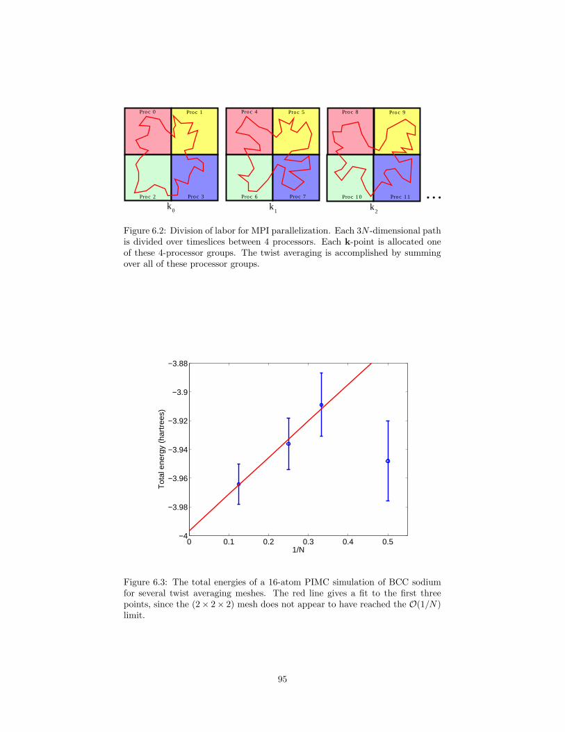
Proc 0 Proc 1

Proc 3Proc 2

Proc 4 Proc 5

Proc 7Proc 6

Proc 8 Proc 9

Proc 1 1Proc 1 0 ...k

0 k1 k

2

Figure 6.2: Division of labor for MPI parallelization. Each 3N -dimensional pathis divided over timeslices between 4 processors. Each k-point is allocated oneof these 4-processor groups. The twist averaging is accomplished by summingover all of these processor groups.

0 0.1 0.2 0.3 0.4 0.5−4

−3.98

−3.96

−3.94

−3.92

−3.9

−3.88

1/N

Tot

al e

nerg

y (h

artr

ees)

Figure 6.3: The total energies of a 16-atom PIMC simulation of BCC sodiumfor several twist averaging meshes. The red line gives a fit to the first threepoints, since the (2× 2× 2) mesh does not appear to have reached the O(1/N)limit.

95

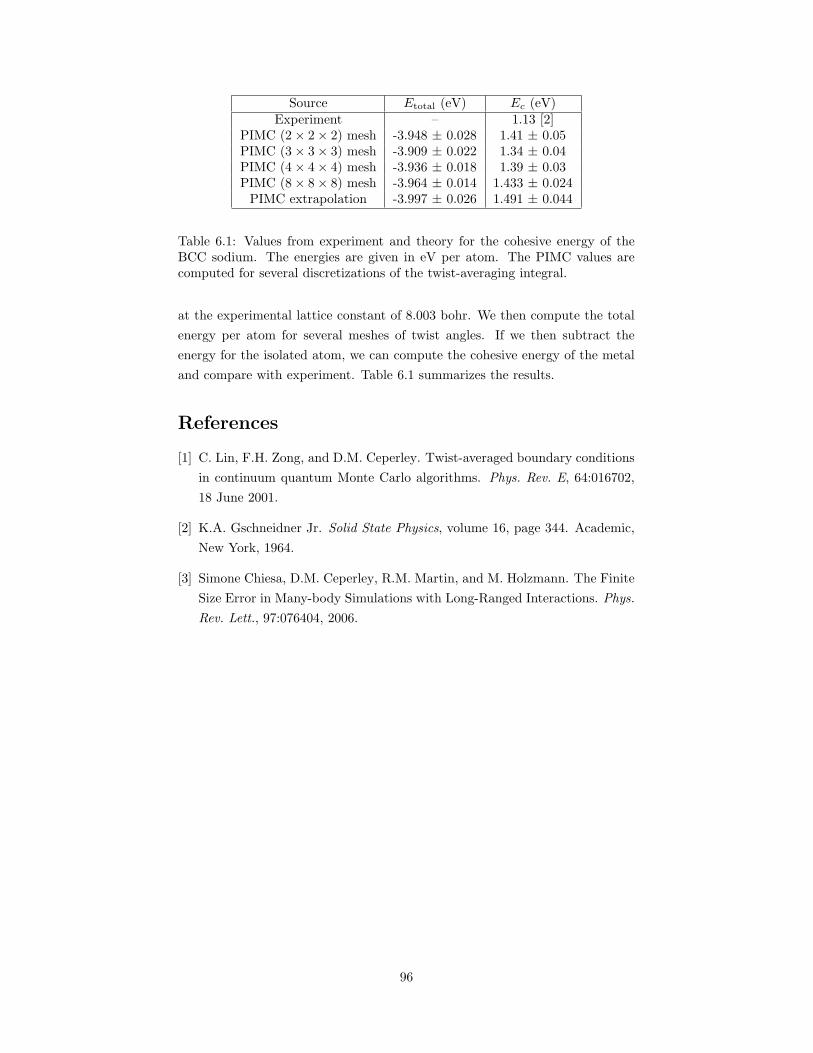
Source Etotal (eV) Ec (eV)Experiment – 1.13 [2]

PIMC (2× 2× 2) mesh -3.948 ± 0.028 1.41 ± 0.05PIMC (3× 3× 3) mesh -3.909 ± 0.022 1.34 ± 0.04PIMC (4× 4× 4) mesh -3.936 ± 0.018 1.39 ± 0.03PIMC (8× 8× 8) mesh -3.964 ± 0.014 1.433 ± 0.024

PIMC extrapolation -3.997 ± 0.026 1.491 ± 0.044

Table 6.1: Values from experiment and theory for the cohesive energy of theBCC sodium. The energies are given in eV per atom. The PIMC values arecomputed for several discretizations of the twist-averaging integral.

at the experimental lattice constant of 8.003 bohr. We then compute the total

energy per atom for several meshes of twist angles. If we then subtract the

energy for the isolated atom, we can compute the cohesive energy of the metal

and compare with experiment. Table 6.1 summarizes the results.

References

[1] C. Lin, F.H. Zong, and D.M. Ceperley. Twist-averaged boundary conditions

in continuum quantum Monte Carlo algorithms. Phys. Rev. E, 64:016702,

18 June 2001.

[2] K.A. Gschneidner Jr. Solid State Physics, volume 16, page 344. Academic,

New York, 1964.

[3] Simone Chiesa, D.M. Ceperley, R.M. Martin, and M. Holzmann. The Finite

Size Error in Many-body Simulations with Long-Ranged Interactions. Phys.

Rev. Lett., 97:076404, 2006.

96

Chapter 7

Fixed-phase path integralMonte Carlo

7.1 Introduction

In 1975, J.B. Anderson introduced the fixed-node method as an approximate so-

lution to the fermion sign problem [4]. In 1980, Ceperley and Alder extended this

method and applied it to the homogeneous electron gas [2]. In the fixed-node

method, one begins with a trial wavefunction, ψT , and stochastically projects

out the lowest energy wave function which shares the same nodes as ψT . With

a reasonable trial wave function, very accurate ground state properties can be

calculated.

The finite-temperature analogue of fixed-node diffusion Monte Carlo is known

as restricted path integral Monte Carlo, or RPIMC. In this method, the sam-

pled paths are a restricted subset of the boson paths. In particular, we define

a trial density matrix, ρT (R,R′;β), and restrict our sampling to paths which

do not cross the 6NM -dimensional nodal surfaces, ρT (R,R′;β) = 0. This con-

straint requires that the sampling of permutations space be restricted to even

permutations.

The fixed-node method, as originally introduced, requires the use of purely

real trial wave functions. The twist-averaging method described in the previous

chapter, however, introduces a twist vector, k, which necessitates the use of a

complex trial function. In 1993, Ortiz, Ceperley, and Martin introduced the

fixed-phase generalization, which allowed systems with complex wave functions

[3]. In this chapter, we discuss how the fixed-phase method can be adapted to

work in path integral Monte Carlo.

7.2 Formalism

We begin by introducing a many-body phase function, Φ(R,R′;β), which we

constrain to be real. We then write our many body density matrix as

ρ(R,R′;β) = ρ(R,R′;β)eiΦ(R,R′;β), (7.1)

97

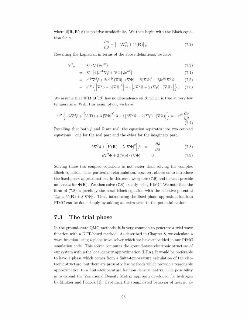
where ρ(R,R′;β) is positive semidefinite. We then begin with the Bloch equa-

tion for ρ,

− ∂ρ

∂β=[−λ∇2

R + V (R)]ρ. (7.2)

Rewriting the Laplacian in terms of the above definitions, we have

∇2ρ = ∇ · ∇(ρeiΦ

)(7.3)

= ∇ ·[i(eiΦ∇ρ+∇Φ

)ρeiΦ

](7.4)

= eiΦ∇2ρ+ 2ieiΦ (∇ρ) · (∇Φ)− ρ |∇Φ|2 + iρeiΦ∇2Φ (7.5)

= eiΦ[

∇2ρ− ρ |∇Φ|2]

+ i[

ρ∇2Φ + 2 (∇ρ) · (∇Φ)]

. (7.6)

We assume that Φ(R,R′;β) has no dependence on β, which is true at very low

temperature. With this assumption, we have

eiΦ

−λ∇2ρ+[

V (R) + λ |∇Φ|2]

ρ+ i[ρ∇2Φ + 2 (∇ρ) · (∇Φ)

]

= −eiΦ ∂ρ

∂β.

(7.7)

Recalling that both ρ and Φ are real, the equation separates into two coupled

equations – one for the real part and the other for the imaginary part,

− λ∇2ρ+[

V (R) + λ |∇Φ|2]

ρ = − ∂ρ∂β

(7.8)

ρ∇2Φ + 2 (∇ρ) · (∇Φ) = 0. (7.9)

Solving these two coupled equations is not easier than solving the complex

Bloch equation. This particular reformulation, however, allows us to introduce

the fixed phase approximation. In this case, we ignore (7.9) and instead provide

an ansatz for Φ(R). We then solve (7.8) exactly using PIMC. We note that the

form of (7.8) is precisely the usual Bloch equation with the effective potential

Veff ≡ V (R) + λ|∇Φ|2. Thus, introducing the fixed phase approximation into

PIMC can be done simply by adding an extra term to the potential action.

7.3 The trial phase

In the ground-state QMC methods, it is very common to generate a trial wave

function with a DFT-based method. As described in Chapter 8, we calculate a

wave function using a plane wave solver which we have embedded in our PIMC

simulation code. This solver computes the ground-state electronic structure of

our system within the local density approximation (LDA). It would be preferable

to have a phase which comes from a finite-temperature calculation of the elec-

tronic structure, but there are presently few methods which provide a reasonable

approximation to a finite-temperature fermion density matrix. One possibility

is to extend the Variational Density Matrix approach developed for hydrogen

by Militzer and Pollock [1]. Capturing the complicated behavior of heavier el-

98

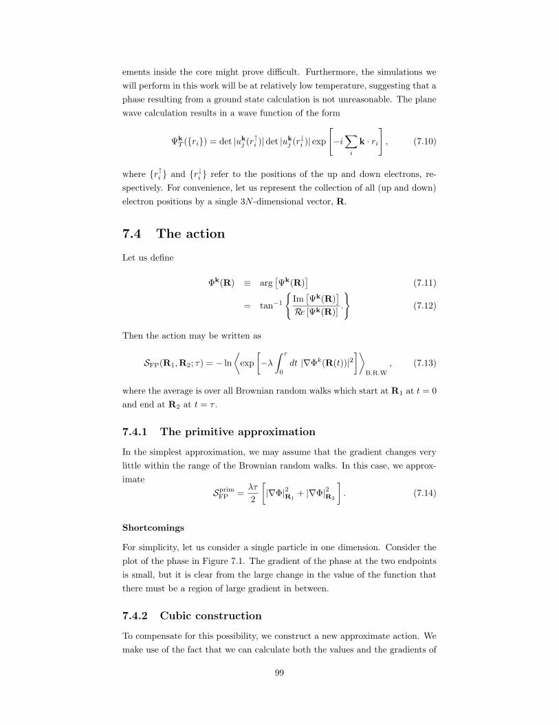
ements inside the core might prove difficult. Furthermore, the simulations we

will perform in this work will be at relatively low temperature, suggesting that a

phase resulting from a ground state calculation is not unreasonable. The plane

wave calculation results in a wave function of the form

ΨkT (ri) = det |uk

j (r↑i )|det |ukj (r↓i )| exp

[

−i∑

i

k · ri]

, (7.10)

where r↑i and r↓i refer to the positions of the up and down electrons, re-

spectively. For convenience, let us represent the collection of all (up and down)

electron positions by a single 3N -dimensional vector, R.

7.4 The action

Let us define

Φk(R) ≡ arg[Ψk(R)

](7.11)

= tan−1

Im[Ψk(R)

]

Re [Ψk(R)].

(7.12)

Then the action may be written as

SFP(R1,R2; τ) = − ln

⟨

exp

[

−λ∫ τ

0

dt |∇Φk(R(t))|2]⟩

B.R.W

, (7.13)

where the average is over all Brownian random walks which start at R1 at t = 0

and end at R2 at t = τ .

7.4.1 The primitive approximation

In the simplest approximation, we may assume that the gradient changes very

little within the range of the Brownian random walks. In this case, we approx-

imate

SprimFP =

λτ

2

[

|∇Φ|2R1+ |∇Φ|2R2

]

. (7.14)

Shortcomings

For simplicity, let us consider a single particle in one dimension. Consider the

plot of the phase in Figure 7.1. The gradient of the phase at the two endpoints

is small, but it is clear from the large change in the value of the function that

there must be a region of large gradient in between.

7.4.2 Cubic construction

To compensate for this possibility, we construct a new approximate action. We

make use of the fact that we can calculate both the values and the gradients of

99

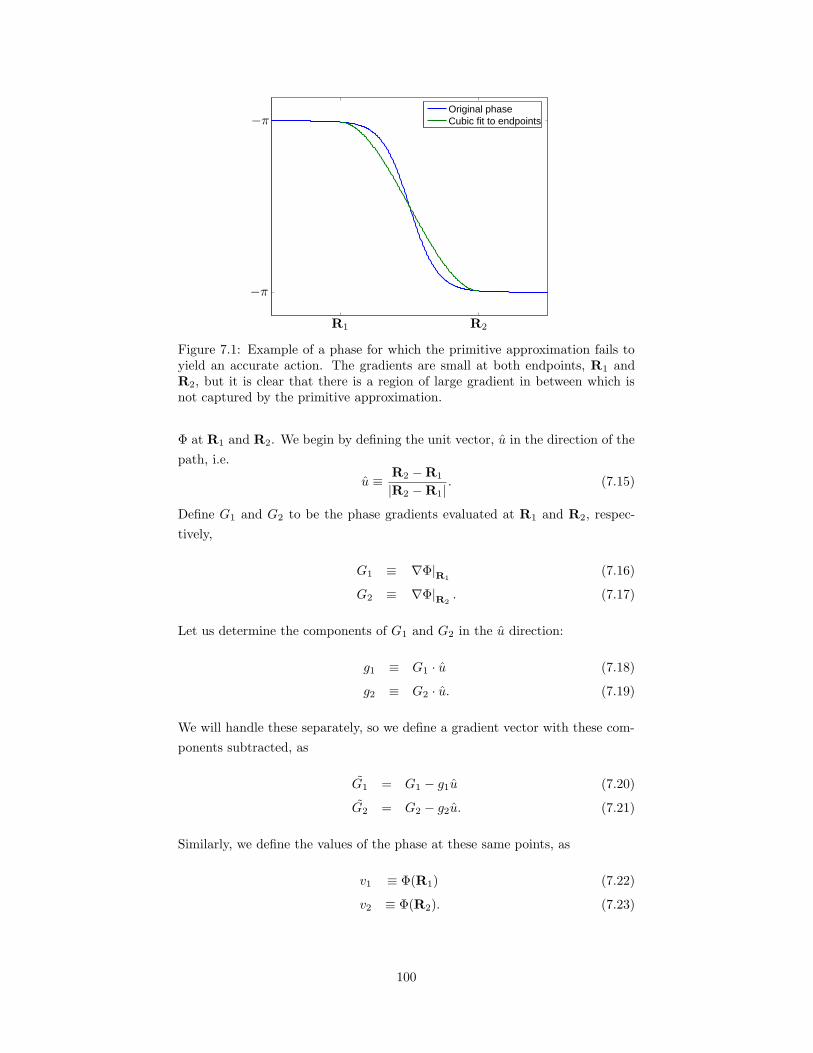
Original phaseCubic fit to endpoints

PSfrag replacements

R1 R2

−π

−π

Figure 7.1: Example of a phase for which the primitive approximation fails toyield an accurate action. The gradients are small at both endpoints, R1 andR2, but it is clear that there is a region of large gradient in between which isnot captured by the primitive approximation.

Φ at R1 and R2. We begin by defining the unit vector, u in the direction of the

path, i.e.

u ≡ R2 −R1

|R2 −R1|. (7.15)

Define G1 and G2 to be the phase gradients evaluated at R1 and R2, respec-

tively,

G1 ≡ ∇Φ|R1(7.16)

G2 ≡ ∇Φ|R2. (7.17)

Let us determine the components of G1 and G2 in the u direction:

g1 ≡ G1 · u (7.18)

g2 ≡ G2 · u. (7.19)

We will handle these separately, so we define a gradient vector with these com-

ponents subtracted, as

G1 = G1 − g1u (7.20)

G2 = G2 − g2u. (7.21)

Similarly, we define the values of the phase at these same points, as

v1 ≡ Φ(R1) (7.22)

v2 ≡ Φ(R2). (7.23)

100

Now, we construct a cubic polynomial representing the phase in the u direction.

We then define the function φ(u), such that

φ(0) = v1 (7.24)

φ(1) = v2 (7.25)

dφ

du

∣∣∣∣0

= g1 (7.26)

dφ

du

∣∣∣∣1

= g2, (7.27)

where g1 = |R2 −R1|g1 and g2 = |R2 −R1|g2. We now write

φ(u) = c3u3 + c2u

2 + c1u+ c0. (7.28)

Solving for cn, yields

c0 = v1 (7.29)

c1 = g1 (7.30)

c2 = 3(v2 − v1)− 2g1 − g2 (7.31)

c3 = (g1 + g2)− 2(v2 − v1) (7.32)

Now, we may calculate the gradient in the u direction:

Gu(u) =1

|R2 −R1|dφ

du(7.33)

=3c3u

2 + 2c2u+ c1|R2 −R1|

. (7.34)

We write our our corrected approximation as

S(R1,R2; τ)corrFP =

λτ

2

[

G21 + G2

2

]

+ λτ

∫ 1

0

duGu(u)2 (7.35)

=λτ

2

[

G21 + G2

2

]

+λτ

|R2 −R1|2× (7.36)

∫ 1

0

du[9c23u

4 + 6c2c3u3 + (4c22 + 3c1c3)u

2 + 2c1c2u+ c21]

= λτ

1

2

[

G21 + G2

2

]

+

[95c

23 + 3

2c2c3 + 43c

22 + c1c3 + c1c2 + c21

]

|R2 −R1|2

. (7.37)

101

Expanding this, we have

Scorrφ (R1,R2; τ) = λτ

1

2

[

G21 + G2

2

]

+ · · ·

2(g21 + g2

2) + 3(g1 + g2)(v1 − v2) + 18(v1 − v2)2 − g1g215 |R2 −R1|2

. (7.38)

As a check of our algebra, we consider the swapping of the 1 and 2 indices.

We recall, then, because of our definitions, g1 and g2 will flip sign. Hence the

3(g1 + g2)(v1 − v2) term will retain its value. Hence, we do have the expected

symmetry under the exchange of labels.

7.5 Calculating phase gradients

We recall that

Φ = arg(Ψ). (7.39)

Then, we can calculate the gradient by

∇Φ = ∇[

tan−1

(ImΨ

ReΨ

)]

(7.40)

=

[

1

1 +(

ImΨReΨ

)2

]

∇(

ImΨ

ReΨ

)

(7.41)

=

[(ReΨ)2

(ReΨ)2 + (ImΨ)2

] ReΨ∇(ImΨ)− ImΨ∇(ReΨ)

(ReΨ)2(7.42)

=ReΨ∇(ImΨ)− ImΨ∇(ReΨ)

|Ψ|2. (7.43)

Since we have written ∇Φ in terms of ∇Ψ, we need only be able to compute

the value and gradient of the wave function. As we shall see in Chapter 8,

we will store the wave functions in a complex tricubic spline representation.

Computing the gradient of wave function is then a simple matter, which is

addressed in Appendix I.

7.6 Connection with fixed-node

At the Γ-point, i.e. k = (0, 0, 0), Ψ(R) can be chosen to be real. In this case,

Φ(R) alternates between the two values of 0 and π, corresponding, of course,

to the positive and negative regions of the wave function. Inside either of these

nodal pockets, the gradient of the phase is identically zero. On the boundary

between them, i.e. the nodes of Ψ(R), the gradient diverges. This results in a

infinite phase action for any paths which cross a nodal surface. In this sense,

the fixed-node restriction (known as the restricted path method in PIMC) is a

special case of the fixed-phase restriction.

102

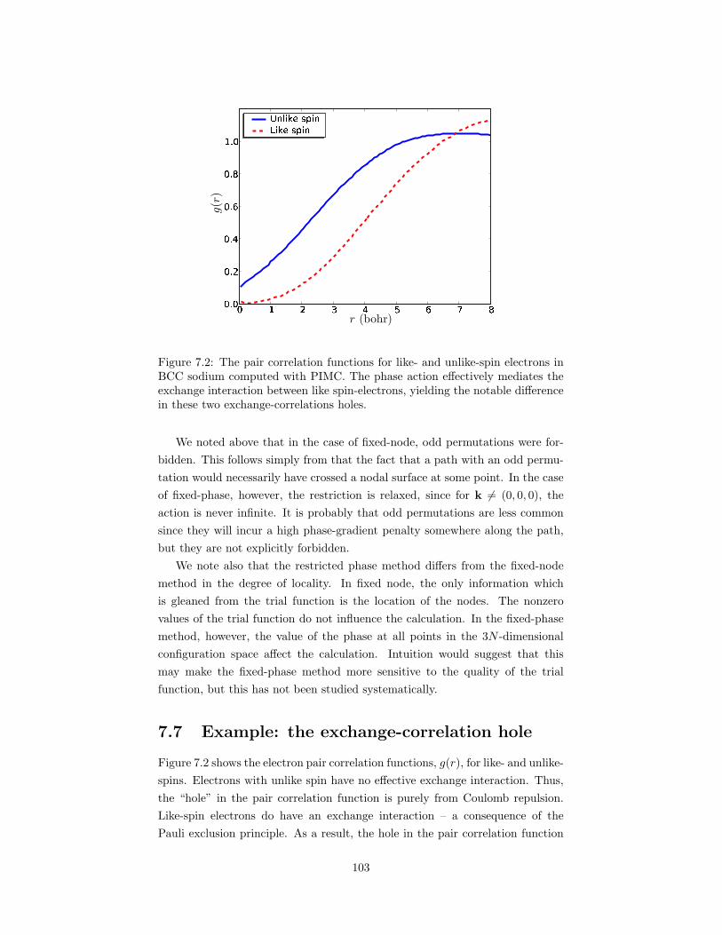
PSfrag replacements

g(r

)

r (bohr)

Figure 7.2: The pair correlation functions for like- and unlike-spin electrons inBCC sodium computed with PIMC. The phase action effectively mediates theexchange interaction between like spin-electrons, yielding the notable differencein these two exchange-correlations holes.

We noted above that in the case of fixed-node, odd permutations were for-

bidden. This follows simply from that the fact that a path with an odd permu-

tation would necessarily have crossed a nodal surface at some point. In the case

of fixed-phase, however, the restriction is relaxed, since for k 6= (0, 0, 0), the

action is never infinite. It is probably that odd permutations are less common

since they will incur a high phase-gradient penalty somewhere along the path,

but they are not explicitly forbidden.

We note also that the restricted phase method differs from the fixed-node

method in the degree of locality. In fixed node, the only information which

is gleaned from the trial function is the location of the nodes. The nonzero

values of the trial function do not influence the calculation. In the fixed-phase

method, however, the value of the phase at all points in the 3N -dimensional

configuration space affect the calculation. Intuition would suggest that this

may make the fixed-phase method more sensitive to the quality of the trial

function, but this has not been studied systematically.

7.7 Example: the exchange-correlation hole

Figure 7.2 shows the electron pair correlation functions, g(r), for like- and unlike-

spins. Electrons with unlike spin have no effective exchange interaction. Thus,

the “hole” in the pair correlation function is purely from Coulomb repulsion.

Like-spin electrons do have an exchange interaction – a consequence of the

Pauli exclusion principle. As a result, the hole in the pair correlation function

103

is larger. In PIMC, the exchange interaction is effectively mediated through the

fixed-phase action we have described in this chapter by enforcing the fermionic

antisymmetry of the trial function.

This completes our discussion of the fixed-phased method in PIMC. In the

next chapter, we will address the methods necessary to compute the wave func-

tion Ψ(R).

References

[1] B. Militzer and E.L. Pollock. Variational Density Matrix Method for Warm

Condensed Matter and Applications to Dense Hydrogen. Phys. Rev. E,

61:3470, 2000.

[2] D.M. Ceperley and B.J. Alder. Ground State of the Electron Gas by a

Stochastic Method. Phys. Rev. Lett., 45(7):566, 18 August 1980.

[3] G. Ortiz, D.M. Ceperley, and R.M. Martin. New Stochastic Method for

Systems with Broken Time-Reversal Symmetry: 2D Fermions in a Magnetic

Field. Phys. Rev. Lett., 71(17):2777, 25 October 1993.

[4] J.B. Anderson. A random-walk simulation of the Schrodinger equation: H+3 .

63(4):1499, 15 August 1975.

104

Chapter 8

Plane wave band structurecalculations

8.1 Introduction

In order to use the fixed-phase restriction in our PIMC simulation, we need a

method to compute reasonable electronic wave functions, parameterized by the

positions of the ions, I and the twist vector, k. We shall call this latter simply

the k-point in this chapter to be more consistent with the electronic structure

community. By “reasonable”, we mean to say that we wish the wave functions

to have the appropriate symmetries and capture the dominant effects of the ion

positions. These goals can be achieved by working in an effective independent-

electron approximation, in which the wave functions can be written as a Slater

determinant of single-particle orbitals,

Ψk(R; I) =

∣∣∣∣∣∣∣∣∣∣∣∣∣

ψ0k(r0) ψ1k(r0) ψ2k(r0) . . . ψNk(r0)

ψ0k(r1) ψ1k(r1) ψ2k(r1) . . . ψNk(r1)

ψ0k(r2) ψ1k(r2) ψ2k(r2) . . . ψNk(r2)...

......

. . ....

ψ0k(rN ) ψ1k(rN ) ψ2k(rN ) . . . ψNk(rN )

∣∣∣∣∣∣∣∣∣∣∣∣∣

, (8.1)

where R ≡ r0 . . . rN are the positions of the electrons, I represents the posi-

tions of the ions, and the ψik(r) are the single particles orbitals, with band index

i and crystal momentum k respectively. We work within the Born-Oppenheimer

approximation in which the electronic wave functions depend parametrically on

the ions, which are treated classically. In the simulations performed in this

work, there are neither magnetic fields nor significant spin-orbit coupling. This

permits us to decompose the Slater determinant above into a product of two

smaller determinants – one for the “up” electrons and one for the “down”,

Ψk(R; I) = det[

ψik

(

r↑j

)]

det[

ψik

(

r↓j

)]

. (8.2)

Thus, to form the many-body wave function with Ne electrons, we must solve

for Ne/2 orbitals.

Each orbital, ψik(r), is expanded in a complete basis which we truncate at an

appropriate size to retain both accuracy and computational tractability. In this

chapter, we discuss how we may determine orbitals which will yield an accurate

105

approximation to the true ground state of the system. Reference [16] contains

both an excellent introduction and a more thorough treatment of much of the

material contained in this chapter.

8.2 Beginnings: eigenvectors of the bare-ion

Hamiltonian

A crude approach to compute the orbitals, ψik(r) is to simply compute the

eigenvectors of the bare-ion Hamiltonian given by

Hbare =1

2∇2 + Vion(r), (8.3)

where

Vion(r) =∑

I∈ions

V PH(r− I). (8.4)

Here we work in atomic units, with ~ = me = qe = 1. In these units, our lengths

are expressed in bohr radii and our energies are given in Hartrees. We expand

ψik(r) in a basis of plane waves, with a reciprocal-space cutoff, kc,

ψik(r) = eik·r∑

|G+k|<kc

cGe−iG·r. (8.5)

We may then solve for the Nelec/2 lowest eigenvectors using the conjugate-

gradient approach described in Section 8.4. We construct the up and down

determinants for use in our PIMC simulation by evaluating these eigenvectors

at the electrons’ positions. We call this approach the bare-ion method of deter-

mining a trial wave function for our fixed-phase restriction.

This method proved to be successful in QMC simulations of dense hydrogen

under high pressure [10]. In these dense, relatively homogeneous conditions, the

behavior of the wave functions is dominated by the scattering of the electrons by

the potential of the ions. In this work, we find that in BCC sodium, the bare-ion

method approach yields very reasonable results. Unfortunately, as we move to

more rarefied systems, such as those found near the liquid-vapor critical point,

the lack of screening in (8.3) has catastrophic consequences. As the simulation

proceeds, the ions begin to aggregate into clusters. With no effective repulsion to

keep them separated, the electrons then cluster into the pockets of low potential

energy at the center of these ion aggregates, leaving other lone ions completely

bare of electron charge. Clearly, this is quite unphysical behavior. To correct

it, we use a density functional theory based method to include the mean-field

replusion and the effects of electron exchange and correlation in an approximate

fashion.

106

8.3 Density functional theory and the local

density approximation

In Chapter 3, we briefly described density functional theory, and in particular,

the local density approximation. Here, we give a bit more background on the

method, and then describe in greater detail the practical aspects of performing

an LDA calculation in a plane wave basis.

In 1964, Hohenberg and Kohn gave a simple proof demonstrating that if one

is given ground-state electron density, n(r), of a system comprised of electrons

and nuclei, one can, in principle, determine all of the properties of the system [15]

exactly. As a corollary, there exists a unique functional of the electron density

which gives the total energy of the system. Since this ground state energy must

be variational, minimizing this functional with respect to the density would then

determine all of the ground-state properties of the system. Unfortunately, the

precise form of this functional is not known, and there is little reason to believe

that the exact form would be possible to write down. Nonetheless, a number of

approximate closed-form functionals have been developed which yield surprising

accuracy.

Perhaps the simplest density functional which has some utility is the Thomas-

Fermi-Dirac (TFD) functional:

ETF[n(r)] =

kinetic︷ ︸︸ ︷

3

10(3π2)

23

∫

d3r n(r)5/3 +

electron-ion︷ ︸︸ ︷∫

Vion(r)n(r) (8.6)

−3

4

(3

π

) 13∫

d3r n(r)43

︸ ︷︷ ︸

exchange

+1

2

∫

d3r d3r′n(r)n(r′)

|r− r′|︸ ︷︷ ︸

Hartree

.

The electron-ion and Hartree interaction terms are exact by definition, but the

kinetic and exchange terms are approximate. In particular, the kinetic energy

term is rather crude, and yields poor results, since it fails to accurately reflect

the kinetic energy of electrons confined in the potential of an ion. For example,

near the nucleus, the behavior of the electronic wave function is dominated by

the nuclear potential and by the electron’s kinetic energy. Since the form of the

kinetic energy in the TFD functional is taken from the homogeneous electron

gas, it fails dramatically to capture the correct behavior in this very nonuniform

region. The functional also completely neglects electron correlation, which plays

a significant role in many systems. Thus, while the TFD functional captures

much of the important behavior of the conduction electrons of simple metals, it

cannot be expected to give reasonable results in systems with less homogeneous

charge density.

This density functional theorem would be little other than a curious sidelight

in condensed matter physics were it not recast in a modified form by Kohn and

107

Sham [18]. In this formulation, the wave function is reintroduced, and com-

bined with a modified density functional. The electronic state is described by a

Slater determinant of noninteracting orbitals in an effective density-dependent

Hamiltonian. The eigenstates of the Hamiltonian are computed, and a new

charge density computed. The Hamiltonian is then updated to reflect the new

charge density. This process is repeated until the charge density becomes self-

consistent, i.e. the charge density which results from the occupied eigenstates of

the Hamiltonian is the same charge density that gave rise to the Hamiltonian.

This innovation makes it possible to create approximations much more ac-

curate than a pure density functional, such as TFD. By reintroducing the wave

function, it becomes possible to accurately reproduce the correct kinetic en-

ergy in regions of highly nonuniform electron density, while at the same time

introducing correlation effects in an average sense.

8.3.1 The Kohn-Sham functional

The Kohn-Sham density functional can be written as

E[n(r)] = Ts[ψi] + EH [n(r)] + EXC [n(r)] +

∫

dr n(r)Vext(r), (8.7)

where the kinetic term, Ts, is given in terms of the wave function by

Ts[ψi] = −1

2

N∑

i=1

∫

dr ψ∗i (r)∇2ψi(r), (8.8)

the Hartree term, EH [n(r)], is given by

EH [n(r)] =1

2

∫

dr dr′n(r)n(r′)

|r− r′| , (8.9)

and the final term for the external potential is usually just the interaction of

the electrons with the ions but may include additional terms, such as those due

to an applied electric field. In the case of bare nuclei, this term is given by

Vion(r) =∑

I∈ions

−ZI

|I− r| . (8.10)

In the context of this dissertation, the external “potential” comes in the form

of pseudohamiltonians. Their application in this context is discussed in sec-

tion 8.5.2.

The term we skipped, EXC [n(r)], is known as the exchange-correlation en-

ergy functional. There are a number of very common formulations, but perhaps

the simplest and most-used is the local density approximation (LDA). In this

108

approximation, EXC is given by

EXC [n(r)] =

∫

dr n(r)εXC(n(r)), (8.11)

where εXC(n) is no longer a functional, but rather a simple function. In particu-

lar, εXC(n) is taken be the total energy density (per electron) of a homogeneous

gas of electrons with density n, less the kinetic and Hartree contributions. This

function is usually written as a parameterization of the data obtained for the

electron gas from QMC simulations by Ceperley and Alder [4]. A number of

parameterizations exist. In this work, we use the Perdew-Zunger form since it

is one of the most commonly cited in the literature [8].

8.3.2 Outline of the iterative procedure

Now that we have a well-defined energy functional, it must be minimized under

the restriction that the integral of the charge density is equal to N , the number

of electrons in the system. The electron density, n(r), can be given in terms of

the wave functions as

n(r) =∑

i,k

fik |ψik(r)|2 , (8.12)

where fik is the occupation of the ith orbital. All quantities in the functional

(8.7) can then be written in terms of the wave function orbitals. If we then

expand each orbital in a basis of plane waves,

ψi(r) =∑

G

ciGeiG·r, (8.13)

the functional may then be written as a function of the ciG coefficients,

E[n(r)] = E(ciG). (8.14)

This function can then be minimized with respect the the plane wave coefficients

subject to the constraint that the orbitals, ψi, remain orthonormal, i.e.

∫

cell

dr ψ∗ik(r)ψjk(r) = δij . (8.15)

Methods exist which directly minimize the energy functional with respect

to the plane wave coefficients, as in (8.14). It is more common, however, to

partition the problem into two nested parts: 1) the solution of the Schrodinger

equation for each orbital given a fixed effective potential, Veff = VH +Vion+VXC ,

and 2) the determination of the density, and resultant effective potential, which

yields self-consistency. We adopt this latter approach.

This two-stage iterative method proceeds as shown schematically in Fig-

ure 8.1. We begin by guessing a form for the charge density, most often taken

to be a superposition of the atomic charge densities. This is known as the input

109

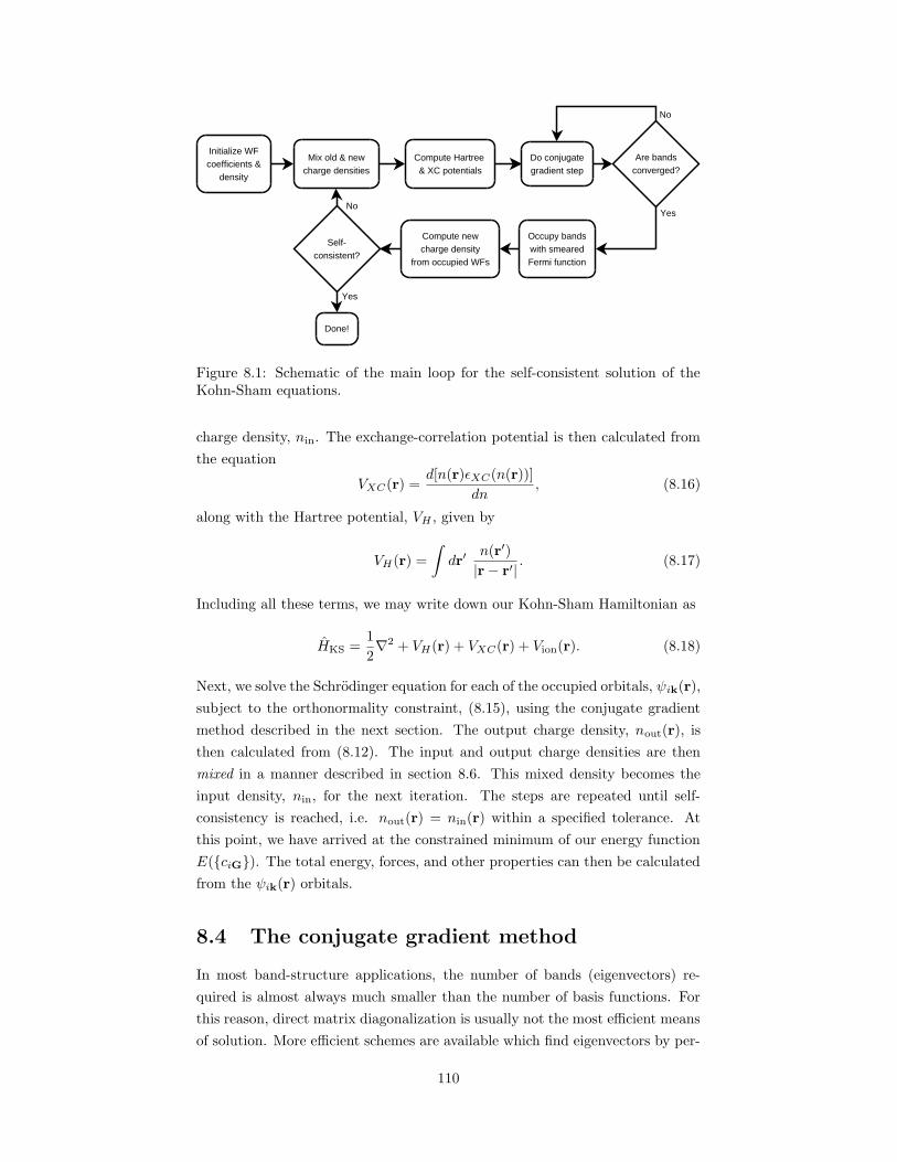
Initialize WFcoefficients &

density

Compute newcharge density

from occupied WFs

Occupy bandswith smearedFermi function

Self-consistent?

Mix old & newcharge densities

Compute Hartree & XC potentials

Do conjugategradient step

Are bandsconverged?

Done!

Yes

NoYes

No

Figure 8.1: Schematic of the main loop for the self-consistent solution of theKohn-Sham equations.

charge density, nin. The exchange-correlation potential is then calculated from

the equation

VXC(r) =d[n(r)εXC(n(r))]

dn, (8.16)

along with the Hartree potential, VH , given by

VH(r) =

∫

dr′n(r′)

|r− r′| . (8.17)

Including all these terms, we may write down our Kohn-Sham Hamiltonian as

HKS =1

2∇2 + VH(r) + VXC(r) + Vion(r). (8.18)

Next, we solve the Schrodinger equation for each of the occupied orbitals, ψik(r),

subject to the orthonormality constraint, (8.15), using the conjugate gradient

method described in the next section. The output charge density, nout(r), is

then calculated from (8.12). The input and output charge densities are then

mixed in a manner described in section 8.6. This mixed density becomes the

input density, nin, for the next iteration. The steps are repeated until self-

consistency is reached, i.e. nout(r) = nin(r) within a specified tolerance. At

this point, we have arrived at the constrained minimum of our energy function

E(ciG). The total energy, forces, and other properties can then be calculated

from the ψik(r) orbitals.

8.4 The conjugate gradient method

In most band-structure applications, the number of bands (eigenvectors) re-

quired is almost always much smaller than the number of basis functions. For

this reason, direct matrix diagonalization is usually not the most efficient means

of solution. More efficient schemes are available which find eigenvectors by per-

110

forming an iterative search to minimize the variational energy. In particular,

Teter, Payne, and Allan introduced a very efficient scheme based on the well-

known conjugate gradients (CG) method [12, 13]. Later work by Kresse and

Furthmuller [6] contains quite useful modifications to this approach. In this

work we use a combination of the methods suggested in these papers.

In the present context, we make use of the variational principle of the

Schrodinger equation, i.e. that the ground state of the Hamiltonian is the one

which minimizes the expectation value of the energy, subject to the constraint of

the orthonormality of the orbitals. The conjugate gradient (CG) method is an

algorithm for nonlinear optimization belonging to the steepest-descents family.

In this family of methods, a search direction is first chosen, usually by taking

the opposite of the gradient of the function to minimize. This direction is called

the direction of steepest descent, since the function decreases most rapidly in

that direction. We then perform a line minimization, i.e. we find the minimum

of the function along the line from the present point in the search direction.

This process is iteratively repeated until the minimum is located within a given

tolerance.

The conjugate gradient method improves upon the steepest-descent algo-

rithm. The first step in each CG iteration is to compute the constrained and

preconditioned steepest descent direction, η′. In the first CG iteration, we min-

imize the energy in the direction of η′. In the succeeding iterations, we again

compute the steepest descent direction, η′, but then we project out the com-

ponent in the direction of the previous search direction. The energy is then

minimized along this new, conjugate search direction, ϕ′. The additional con-

jugacy step prevents the new search from undoing the optimizations of the

previous one. It can be shown that if the energy is quadratic in the wave func-

tion coefficients, the exact minimum of an N -dimensional vector space can be

found in N iterations. In practice, the minimum is found to very high accuracy

in far fewer iterations.

In the procedure we describe below, we largely follow the method outlined in

reference [12], with a few modifications. We adopt their notation for consistency

and clarity. We denote each orbital as ψik, where i is again the band index the

k is the twist vector in the first Brillouin zone. Computationally, ψik is stored

as a vector of plane-wave coefficients, ckiG.

For the moment, we will drop the twist parameter to avoid cumbersome no-

tation. In each iteration, we begin by computing the steepest-descent direction

for band i, ξi,

ξ = E0ψ − HKSψ, (8.19)

where E0 plays the role of a Lagrange multiplier preserving the normalization

of the vector and is given by

E0 = 〈ψ|HKS|ψ〉. (8.20)

111

The steepest descent vector is then made orthogonal to all the bands in order

to retain the band orthogonality, via

ξ′ = ξ −∑

j

〈ψj |ξi〉ψj . (8.21)

This steepest descent vector gives the direction in which the energy decreases

most rapidly, but we prefer the direction in which the error in the wave function

decreases fastest. We can modify the search direction to be closer to this opti-

mal direction through a process known as preconditioning. The preconditioned

search direction, η, can be obtained by multiplying by the matrix, KG,G′ ,

KG,G′ = δG,G′

27 + 18x+ 12x2 + 8x3

27 + 18x+ 12x2 + 8x3 + 16x4, (8.22)

where

x =|k + G|2〈ψi|∇2|ψi〉

. (8.23)

The motivation for this form for the preconditioner is given in [12]. The precon-

ditioning will not maintain the orthogonality to the bands, so the preconditioned

direction, ηi is again orthogonalized to all the bands as in (8.21), yielding η′i.

Next, we must determine the conjugate search direction, ϕi. That is, we

wish to keep the current search direction orthogonal to all previous search di-

rections. Let the superscript p denote vectors from the previous CG iteration.

The conjugate direction is then written as

ϕi = η′i + γiϕpi , (8.24)

where

γi =〈η′i|ξi〉〈η′pi |ξ′

pi 〉. (8.25)

Finally, ϕi is once more orthogonalized to all the bands and then normalized,

yielding our final search direction, ϕ′i.

Next, we must minimize the energy along the search direction. We write the

band for the next iteration, ψni , in the form

ψni = ψi cos θ + ϕ′

i sin θ, (8.26)

which preserves the normalization. This reduces the line minimization to finding

the value of θ that minimizes E(θ), which is given as

E(θ) = 〈ψi cos θ + ϕ′i sin θ|HKS|ψi cos θ + ϕ′

i sin θ〉. (8.27)

It would be very costly to minimize E(θ) exactly through, say, a bisection search.

112

Rather, we write an ansatz for the form of E as

E(θ) = E +A cos(2θ) +B sin(2θ), (8.28)

where E is the average value of E(θ), and A and B are constants which can

be written in terms of the first two derivatives of E. We can then compute the

value of θ which minimizes our ansatz,

θmin =1

2tan−1

(

−∂E∂θ

∣∣θ=0

12

∂2E∂θ2

∣∣θ=0

)

. (8.29)

The first derivative of the energy is given simply as

∂E

∂θ= 2Re

⟨

ϕ′i|HKS|ψi

⟩

, (8.30)

while the second is given by

∂2E

∂θ2= 2

[

Re⟨

ϕ′i|HKS|ψi

⟩

− 〈ψi|H|ψi〉]

. (8.31)

After θmin is determined, we update ψi according to (8.26). This completes

one conjugate gradient iteration for band i. The CG iterations proceed until

the norm of the residual vector, ξ′i, falls below a given tolerance for all occu-

pied bands, i. The charge density is then updated, the Hartree and exchange-

correlation potentials are recomputed, and then the next set of CG iterations

begin.

In the present work, we parallelize the CG minimizations over bands, with

each processor being allocated Nbands/Nprocs bands. Each processor loops over

each of the bands it has been allocated before proceeding to the next CG iter-

ation. Thus, the algorithm we employ falls into the category of an all-bands-

simultaneously algorithm. Other algorithms, known as band-by-band fully con-

verge each band before proceeding to the next band.

8.4.1 Subspace rotation

The CG algorithm given above will not, as stated, converge to the final Kohn-

Sham eigenvectors, since the algorithm minimizes the total energy for the sys-

tem, which is invariant to unitary rotations within the occupied subspace. In

order to find the Kohn-Sham eigenvectors, we must then perform a subspace

diagonalization. We therefore compute the subspace Hamiltonian, H sub, whose

elements are given by

Hsubij = 〈ψi|HKS|ψj〉. (8.32)

Since this matrix of size Nbands × Nbands is very small in comparison to HKS,

we can use a standard iterative matrix diagonalizer, such as the ZHEEVR sub-

routine of LAPACK. This yields a matrix of subspace eigenvector coefficients,

113

αij , which optimally rotate the subspace through the relation

ψ′i =

∑

j

αijψj . (8.33)

In the present work, we perform a subspace rotation after each update of the

effective potentials, VH and VXC . We find that doing so significantly reduces

the number of cycles required to converge the occupied bands. Futhermore, it

prevents an instability that can result from the reordering of the bands when

the Hamiltonian is updated.

To see how, consider the ith orbital, ψi. Before it has reached convergence,

it will contain components of the true eigenstate, ψ0i , and higher energy eigen-

states, ψ0j ,

ψi = αiψ0i +

∑

j>i

αjψ0j . (8.34)

Each of the ψj ’s will be projected out from ψi by the CG iterations at a rate

proportional to the eigenvalue difference, Ej − Ei. Thus the state in the sum

with energy closest to ψi will be projected out most slowly by the CG iterations.

Subspace rotation very nearly eliminates the ψ0j components of ψi for all the

bands that are included in our calculation. Thus, including a few unoccupied

bands in the calculation decreases the number of iterations needed to converge

the occupied bands.

8.5 Using FFTs

A conjugate gradient approach has the additional advantage that the Hamil-

tonian need not be explicitly stored in memory. Rather, it requires only that

we can apply HKS to ψi. As the number of plane waves gets large, storing

HKS could be a severe limitation. As we shall see, this operation can be done

extremely efficiently using Fast Fourier Transforms (FFTs).

Applying a general operator in an N -element linear basis usually requires

O(N2) operations. If the operator is diagonal in the present basis (i.e. its own

eigenbasis), however, only O(N) operations are necessary, saving a significant

amount of CPU time. Unfortunately, in the general case, a change of basis

also takes O(N2) time, eliminating the savings. In the case of the plane-wave

band structure methods, all the operators we need to apply are diagonal in

either real space or reciprocal space. Fortunately, there exist algorithms which

exploit the special symmetries of plane waves to change between these two

bases in O[N log(N)] operations. These algorithms are known as Fast Fourier

Transforms (FFTs), and their use is the key to obtaining good performance for

plane-wave methods.

We first begin by defining the Fourier transforms which we will require. For

114

a generic quantity f(r) defined within the simulation cell, we have

fG =1

Ω

∫

dr eiG·rf(r) (8.35)

f(r) =∑

G

e−iG·rfG. (8.36)

We can use a Fast Fourier Transform routine to perform both the real-to-

reciprocal and reciprocal-to-real transforms. A standard 3D FFT routine will

perform the summation

fkxkykz=

Nx−1∑

jx=0

Ny−1∑

jy=0

Nz−1∑

jz=0

fjxjyjzexp

[

±2πi

(jxkx

Nx+jyky

Ny+jzkz

Nz

)]

. (8.37)

If we discretize our simulation cell in real space into Nx ×Ny ×Nz grid points,

we can rewrite our Fourier transforms (8.35-8.36) in this form. For a simulation

cell with dimensions (Lx, Ly, Lz), we write

rjxjyjz=jxLx

Nxx +

jyLx

Nyy +

jzLx

Nzz. (8.38)

Our reciprocal lattice vectors can be written similarly,

Gkxkykz=

2πkx

Lxx +

2πky

Lyy +

2πkz

Lzz. (8.39)

The real-to-reciprocal transform can then be written

fG =LxLyLz

NxNyNz

Nx−1∑

kx=0

Ny−1∑

ky=0

Nz−1∑

kz=0

f(rjxjyjz) exp

[

2πi

(jxkx

Nx+jyky

Ny+jzkz

Nz

)]

,

(8.40)

where G is given by (8.39). The reciprocal-to-real transform is given by

f(rjxjyjz) =

Nx−1∑

kx=0

Ny−1∑

ky=0

Nz−1∑

kz=0

fG exp

[

−2πi

(jxkx

Nx+jyky

Ny+jzkz

Nz

)]

. (8.41)

This can be trivially generalized to non-orthorhombic simulation cells. If Nx,

Ny, and Nz are chosen large enough to contain all the vectors in the summation

(8.36), the FFT versions give exact results for both transforms. The great ad-

vantage of the FFT comes in speed. While a general change of basis operation

with NxNyNz elements would take order (NxNyNz)2 arithmetic operations, the

special symmetries of the plane wave basis are exploited to complete the trans-

form in order NxNyNz log(NxNyNz) operations. Highly optimized libraries are

available which compute the 3D FFTs very efficiently on a range of hardware

platforms. In this work we use the FFTW package [5].

Now that we have seen how Fourier transforms can be done very efficiently,

we show how this can be exploited to save time in our plane wave calculations.

115

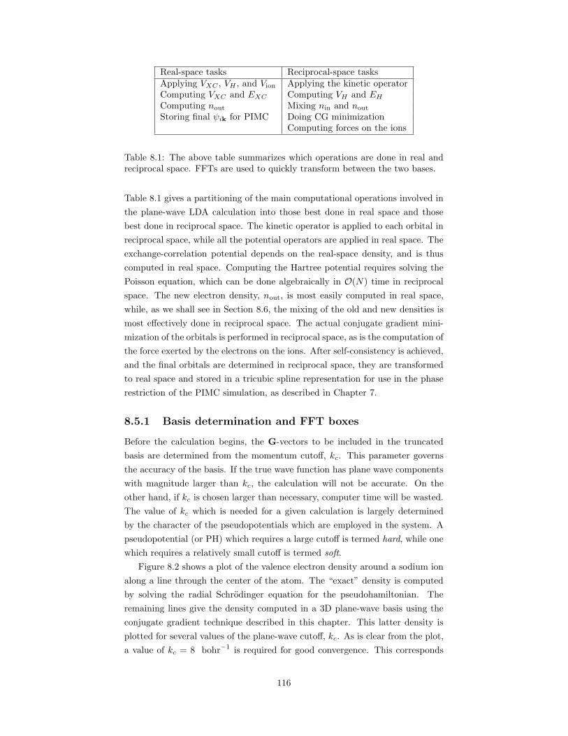
Real-space tasks Reciprocal-space tasksApplying VXC , VH , and Vion Applying the kinetic operatorComputing VXC and EXC Computing VH and EH

Computing nout Mixing nin and nout

Storing final ψik for PIMC Doing CG minimizationComputing forces on the ions

Table 8.1: The above table summarizes which operations are done in real andreciprocal space. FFTs are used to quickly transform between the two bases.

Table 8.1 gives a partitioning of the main computational operations involved in

the plane-wave LDA calculation into those best done in real space and those

best done in reciprocal space. The kinetic operator is applied to each orbital in

reciprocal space, while all the potential operators are applied in real space. The

exchange-correlation potential depends on the real-space density, and is thus

computed in real space. Computing the Hartree potential requires solving the

Poisson equation, which can be done algebraically in O(N) time in reciprocal

space. The new electron density, nout, is most easily computed in real space,

while, as we shall see in Section 8.6, the mixing of the old and new densities is

most effectively done in reciprocal space. The actual conjugate gradient mini-

mization of the orbitals is performed in reciprocal space, as is the computation of

the force exerted by the electrons on the ions. After self-consistency is achieved,

and the final orbitals are determined in reciprocal space, they are transformed

to real space and stored in a tricubic spline representation for use in the phase

restriction of the PIMC simulation, as described in Chapter 7.

8.5.1 Basis determination and FFT boxes

Before the calculation begins, the G-vectors to be included in the truncated

basis are determined from the momentum cutoff, kc. This parameter governs

the accuracy of the basis. If the true wave function has plane wave components

with magnitude larger than kc, the calculation will not be accurate. On the

other hand, if kc is chosen larger than necessary, computer time will be wasted.

The value of kc which is needed for a given calculation is largely determined

by the character of the pseudopotentials which are employed in the system. A

pseudopotential (or PH) which requires a large cutoff is termed hard, while one

which requires a relatively small cutoff is termed soft.

Figure 8.2 shows a plot of the valence electron density around a sodium ion

along a line through the center of the atom. The “exact” density is computed

by solving the radial Schrodinger equation for the pseudohamiltonian. The

remaining lines give the density computed in a 3D plane-wave basis using the

conjugate gradient technique described in this chapter. This latter density is

plotted for several values of the plane-wave cutoff, kc. As is clear from the plot,

a value of kc = 8 bohr−1 is required for good convergence. This corresponds

116

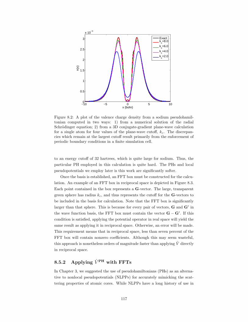
−10 −5 0 5 100

0.5

1

1.5

2

2.5

3

x 10−3

x (bohr)

n(x)

Exactk

c=8.0

kc=6.0

kc=4.0

kc=2.0

Figure 8.2: A plot of the valence charge density from a sodium pseudohamil-tonian computed in two ways: 1) from a numerical solution of the radialSchrodinger equation; 2) from a 3D conjugate-gradient plane-wave calculationfor a single atom for four values of the plane-wave cutoff, kc. The discrepan-cies which remain at the largest cutoff result primarily from the enforcement ofperiodic boundary conditions in a finite simulation cell.

to an energy cutoff of 32 hartrees, which is quite large for sodium. Thus, the

particular PH employed in this calculation is quite hard. The PHs and local

pseudopotentials we employ later is this work are significantly softer.

Once the basis is established, an FFT box must be constructed for the calcu-

lation. An example of an FFT box in reciprocal space is depicted in Figure 8.3.

Each point contained in the box represents a G-vector. The large, transparent

green sphere has radius kc, and thus represents the cutoff for the G-vectors to

be included in the basis for calculation. Note that the FFT box is significantly

larger than that sphere. This is because for every pair of vectors, G and G′ in

the wave function basis, the FFT box must contain the vector G −G′. If this

condition is satisfied, applying the potential operator in real space will yield the

same result as applying it in reciprocal space. Otherwise, an error will be made.

This requirement means that in reciprocal space, less than seven percent of the

FFT box will contain nonzero coefficients. Although this may seem wasteful,

this approach is nonetheless orders of magnitude faster than applying V directly

in reciprocal space.

8.5.2 Applying V PH with FFTs

In Chapter 3, we suggested the use of pseudohamiltonians (PHs) as an alterna-

tive to nonlocal pseudopotentials (NLPPs) for accurately mimicking the scat-

tering properties of atomic cores. While NLPPs have a long history of use in

117

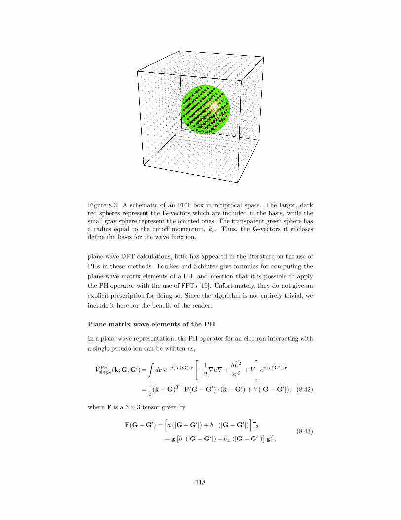
Figure 8.3: A schematic of an FFT box in reciprocal space. The larger, darkred spheres represent the G-vectors which are included in the basis, while thesmall gray sphere represent the omitted ones. The transparent green sphere hasa radius equal to the cutoff momentum, kc. Thus, the G-vectors it enclosesdefine the basis for the wave function.

plane-wave DFT calculations, little has appeared in the literature on the use of

PHs in these methods. Foulkes and Schluter give formulas for computing the

plane-wave matrix elements of a PH, and mention that it is possible to apply

the PH operator with the use of FFTs [19]. Unfortunately, they do not give an

explicit prescription for doing so. Since the algorithm is not entirely trivial, we

include it here for the benefit of the reader.

Plane matrix wave elements of the PH

In a plane-wave representation, the PH operator for an electron interacting with

a single pseudo-ion can be written as,

V PHsingle(k;G,G′) =

∫

dr e−i(k+G)·r[

−1

2∇a∇+

bL2

2r2+ V

]

ei(k+G′)·r

=1

2(k + G)T · F(G−G′) · (k + G′) + V (|G−G′|), (8.42)

where F is a 3× 3 tensor given by

F(G−G′) =[

a (|G−G′|) + b⊥ (|G−G′|)]

3

+ g[b‖ (|G−G′|)− b⊥ (|G−G′|)

]gT ,

(8.43)

118

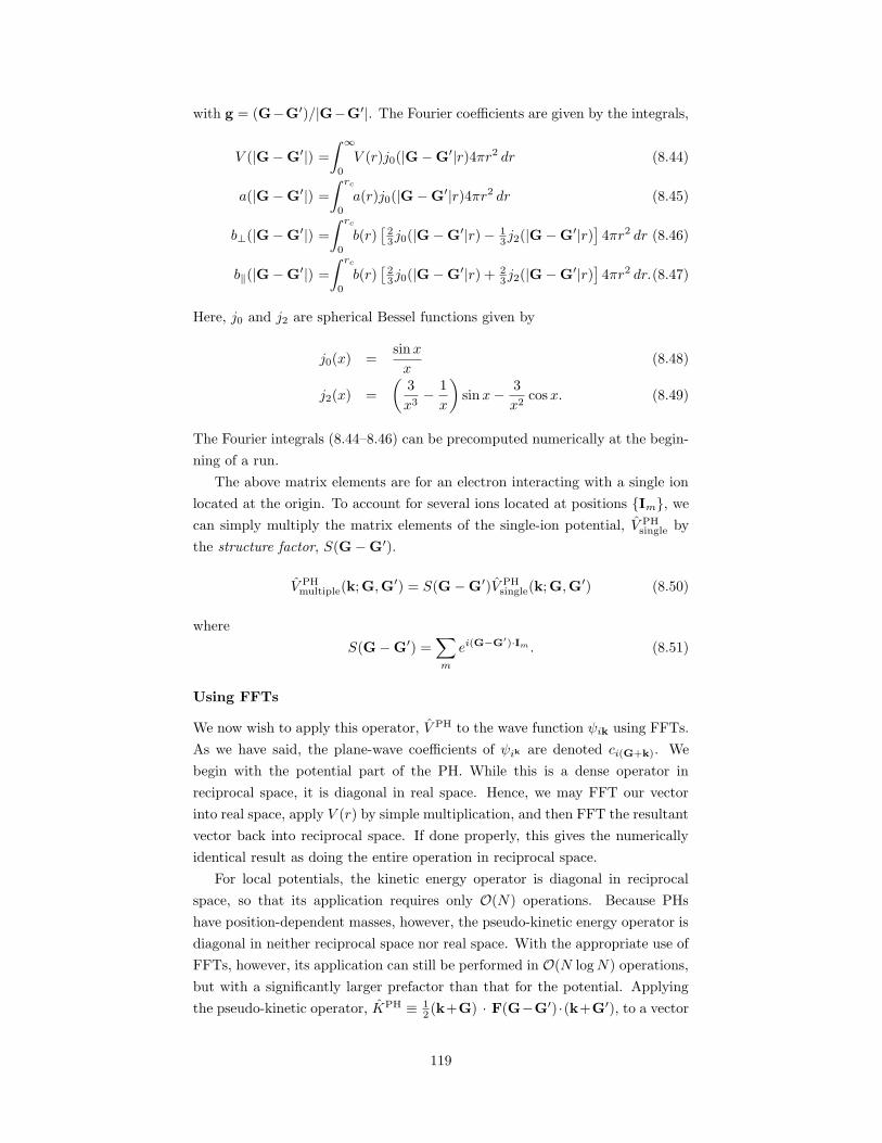
with g = (G−G′)/|G−G′|. The Fourier coefficients are given by the integrals,

V (|G−G′|) =

∫ ∞

0

V (r)j0(|G−G′|r)4πr2 dr (8.44)

a(|G−G′|) =

∫ rc

0

a(r)j0(|G−G′|r)4πr2 dr (8.45)

b⊥(|G−G′|) =

∫ rc

0

b(r)[

23j0(|G−G′|r)− 1

3j2(|G−G′|r)]4πr2 dr (8.46)

b‖(|G−G′|) =

∫ rc

0

b(r)[

23j0(|G−G′|r) + 2

3j2(|G−G′|r)]4πr2 dr.(8.47)

Here, j0 and j2 are spherical Bessel functions given by

j0(x) =sinx

x(8.48)

j2(x) =

(3

x3− 1

x

)

sinx− 3

x2cosx. (8.49)

The Fourier integrals (8.44–8.46) can be precomputed numerically at the begin-

ning of a run.

The above matrix elements are for an electron interacting with a single ion

located at the origin. To account for several ions located at positions Im, we

can simply multiply the matrix elements of the single-ion potential, V PHsingle by

the structure factor, S(G−G′).

V PHmultiple(k;G,G′) = S(G−G′)V PH

single(k;G,G′) (8.50)

where

S(G−G′) =∑

m

ei(G−G′)·Im . (8.51)

Using FFTs

We now wish to apply this operator, V PH to the wave function ψik using FFTs.

As we have said, the plane-wave coefficients of ψik are denoted ci(G+k). We

begin with the potential part of the PH. While this is a dense operator in

reciprocal space, it is diagonal in real space. Hence, we may FFT our vector

into real space, apply V (r) by simple multiplication, and then FFT the resultant

vector back into reciprocal space. If done properly, this gives the numerically

identical result as doing the entire operation in reciprocal space.

For local potentials, the kinetic energy operator is diagonal in reciprocal

space, so that its application requires only O(N) operations. Because PHs

have position-dependent masses, however, the pseudo-kinetic energy operator is

diagonal in neither reciprocal space nor real space. With the appropriate use of

FFTs, however, its application can still be performed in O(N logN) operations,

but with a significantly larger prefactor than that for the potential. Applying

the pseudo-kinetic operator, KPH ≡ 12 (k+G) · F(G−G′) ·(k+G′), to a vector

119

of wave function coefficients, c, can be accomplished through the following steps:

1. Compute the F(G−G′) tensor in reciprocal space.

2. FFT the tensor into real space.

3. Multiply each wave function plane-wave coefficient, cG+k by (k + G′),

yielding a 3×N component vector.

4. FFT this 3×N component vector to real space. The result is the gradient

of c(r), which we denote (∇c)(r).

5. Apply the 3× 3 tensor F(r) to (∇c)(r).

6. Inverse FFT back into reciprocal space. Call this (Fc)G.

7. Finally dot each three-component vector, (Fc)G with 12 (k + G) to yield

(KPHc)G.

The result of these steps is KPHc given in reciprocal space. Note that steps 1

and 2 need only be performed each time the ion positions or k-point are changed.

8.6 Achieving self-consistency: charge mixing

schemes

Figure 8.1 shows a simplified representation of the main loops of a self-consistent

LDA band structure calculation. The outer self-consistency loop is needed to

ensure that the occupied orbitals, ψi, which are eigenstates of HKS, yield the

same density as that from which HKS was derived.

In the most naive approach, we start with a guess for the density. We then

construct VH and VXC and solve for the occupied bands with conjugate gradi-

ents. We construct a new density from the computed wave functions and repeat

the process. Unfortunately, this approach is very unstable and convergence is

almost never reached.

Linear mixing

The issue of stability arises from a problem of charge oscillation. It most of-

ten occurs that when the Hamiltonian is updated and new occupied orbitals

determined, the new charge density, nout, is quite different from the previous

charge density, nin. The Hamiltonian is again updated, new wave functions

computed, and a new resultant charge density constructed, which again leads

to a quite different charge density. In the naive scheme, this usually yields a

cyclic oscillation of the charge which never converges.

The first approach to correct this problem is known as linear mixing. In this

scheme, the input and output densities, nin and nout, are linearly mixed and

120

the resultant sent to the next self-consistent iteration, i.e.

n∗(r) = αnout(r) + (1− α)nin(r). (8.52)

If α is chosen small enough, the oscillations are suppressed, and convergence is

eventually reached.

Kerker mixing

Unfortunately, as the system size increases, α must be chosen smaller and

smaller to achieve prevent charge oscillation, and convergence becomes slower

and slower. It is noted, however, that the oscillation of the charge comes from

the small G components of the charge. In 1980, Kerker introduced a scheme

which makes the mixing coefficient wavelength-dependent [7]. We may write

n∗G = γ (|G|)noutG +

[1− γ (|G|)

]ninG, (8.53)

where

γ(G) =αG2

G2 + λ2, (8.54)

and λ is a parameter, which must be chosen appropriately. A value from 0.6 to

0.8 bohr−1 is typical. For G λ, very little of the new charge will be mixed in,

greatly stabilizing the self-consistent loop by damping out the charge oscillation.

Advanced methods

More advanced methods exist which make use of the charge densities from all of

the self-consistent iterations. Two are of particular note. The original method of

Broyden was successively improved by Vanderbilt, Louie, and Johnson [3]. An

alternative scheme based on the solution of the Thomas-Fermi-von Weizsacker

equation is given by Raczkowski, Canning, and Wang [1]. This latter method

is particularly useful in converging systems with large simulation cells. In this

work, we use relatively small simulation cells and found the simple Kerker mixing

sufficient for our purposes.

8.7 Wave function initialization

A number of approaches have been suggested for initializing the plane wave

coefficients prior to optimization with conjugate gradients. It is essential that

the initial wave functions are not orthogonal to the true ground state. As a

simple way of ensuring this, Payne et al. [12] suggest using random values.

Other authors have used the converged coefficients from a nearby set of ion

coordinates from a calculation already performed. While this latter approach

has some speed advantage with molecular dynamics, one must take care to avoid

121

instabilities when energy levels cross. In our approach, the subspace rotation

technique prevents this instability.

A technique is still required to initialize the wave functions for the very first

configuration of the ions. The method used in this work was suggested by De-

laney [9]. In this approach, an explicit matrix representation of the Hamiltonian

for an extremely small plane-wave cutoff is constructed and diagonalized with

a standard LAPACK iterative diagonalizer. The result of this calculation de-

termines the initial low-energy plane-wave coefficients for the full Hamiltonian.

All other coefficients are set to a small random value. Finally, the bands are

orthogonalized. This approach for initialization consistently yielded robust and

fast convergence to the ground state.

8.8 Energy level occupation

After solving for the eigenvectors of our Kohn-Sham Hamiltonian, we must

occupy the bands appropriately. In a naive implementation for a system of Ne

electrons and Nk k-points, we would occupy the lowest 12Nk ×Ne energy levels

with 2/Nk electrons each. This works reasonably well with large-gap insulators.

Unfortunately, with metals, this yields practical difficulties with achieving self-

consistency. In particular, it frequently occurs that after updating VH and VXC

in a self-consistent iteration, near-degenerate levels near the Fermi surface switch

ordering, so that a level which was previously occupied becomes unoccupied, and

vice-versa. This problem results in the charge in the system oscillating between

two or more states, preventing convergence.

The well-established solution to this charge sloshing problem is known as

Fermi smearing. At zero temperature, the Fermi function is, of course, a step

function. If we replace this function with a similar one which is smooth at the

Fermi surface, we can eliminate the sloshing problem. A very popular approach

is given by Methfessel and Paxton [11]. We may write the zero-temperature

occupation, fik, as a Fermi function of the eigenenergy, εik,

fik = SF (εik), (8.55)

where the Fermi step function can be written as

SF(ε) = 1−∫ ε

−∞dε δ(ε− µ), (8.56)

where µ is the chemical potential or Fermi energy. We can then expand the

δ-function as a sum of Hermite polynomials with a given width, σ. Performing

122

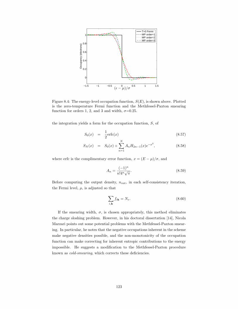
−1.5 −1 −0.5 0 0.5 1 1.5

0

0.2

0.4

0.6

0.8

1

Occ

upan

cy (

elec

tron

s)

T=0 FermiMP order=1MP order=2MP order=3

PSfrag replacements

(ε− µ)/σ

Figure 8.4: The energy-level occupation function, S(E), is shown above. Plottedis the zero-temperature Fermi function and the Methfessel-Paxton smearingfunction for orders 1, 2, and 3 and width, σ=0.25.

the integration yields a form for the occupation function, S, of

S0(x) =1

2erfc(x) (8.57)

SN (x) = S0(x) +

N∑

n=1

AnH2n−1(x)e−x2

, (8.58)

where erfc is the complimentary error function, x = (E − µ)/σ, and

An =(−1)n

n!4n√π. (8.59)

Before computing the output density, nout, in each self-consistency iteration,

the Fermi level, µ, is adjusted so that

∑

i,k

fik = Ne. (8.60)

If the smearing width, σ, is chosen appropriately, this method eliminates

the charge sloshing problem. However, in his doctoral dissertation [14], Nicola

Marzari points out some potential problems with the Methfessel-Paxton smear-

ing. In particular, he notes that the negative occupations inherent in the scheme

make negative densities possible, and the non-monotonicity of the occupation

function can make correcting for inherent entropic contributions to the energy

impossible. He suggests a modification to the Methfessel-Paxton procedure

known as cold-smearing, which corrects these deficiencies.

123

8.9 Molecular dynamics extrapolation

When performing molecular dynamics (MD) simulations, each succeeding con-

figuration of the ions is highly correlated with the previous one. It is possible

to make use of this correlation to greatly improve the starting point of the elec-

tronic structure calculation. In particular, it is possible to extrapolate the wave

functions from the previous two MD steps to create a starting point for the

present step. [17] gives an optimal way of doing so.

A similar scheme can be used to extrapolate the density, but an even more

effective approach for density was given by Alfe [2]. In this approach, the sum

of the electron densities for each atom is subtracted from the total density of the

previous two configurations. The resulting charge difference is then extrapolated

as above, and, finally, the atomic charge for the new configuration is added on.

For the systems studied in this work, we find the simple density extrapolation

of [17] sufficient.

8.10 Validation: BCC sodium bands

Figure 3.6 shows a plot of the band structure of BCC sodium as computed

within LDA. Shown in red are bands computed with the open-source ABINIT

software package using a standard NLPP. The blue curve gives the same curve

computed with a PH and using the methods described in this chapter. Finally,

for comparison, the free-electron bands have also been plotted. While there are

some visible differences resulting from the difference between the PH and NLPP,

there is quite reasonable agreement overall.

In order to ensure that the methods described in this chapter were imple-

mented without error, a comparison was also made between the results from

ABINIT and the embedded code of the present work for a local pseudopoten-

tial that could be used in both codes. The methods were use to compute the

energy for a configuration of sixteen sodium atoms taken from a Langevin dy-

namics simulation, which is described in the next chapter. Each of the energy

components were compared and found to be in agreement to less than 10−6

hartrees.

8.11 Computing forces on the ions

In the next chapter, we discuss the coupling of a PIMC simulation for the

electrons to a molecular-dynamics-like simulation for the sodium ions. As such,

it is very useful to have the capability to compute the forces on the ions for a

given configuration. In this section, we show how this can be done efficiently

within the plane-wave formulation developed in this chapter.

124

8.11.1 Force from the electrons

The Hellman-Feynman theorem states that if the Hamiltonian, H, depends on

some parameter, λ, then the first order change in the expected value of the

energy is given simply by

d

dλ〈ψ|H|ψ〉 =

⟨

ψ

∣∣∣∣∣

dH

dλ

∣∣∣∣∣ψ

⟩

. (8.61)

Since only the external potential, Vion depends on the ion positions, we may

write the expectation value of the energy as,

〈Vion〉 =∑

ik

S(εik)〈ψik|Vion|ψik〉 (8.62)

=∑

ik

∫

d3rψ∗ik(r)Vion(r)ψik(r) (8.63)

=

∫

d3rVion(r)∑

ik

fik|ψik(r)|2 (8.64)

=

∫

d3rVion(r)n(r) (8.65)

=

∫

d3r∑

G,G′

(nGe

−iG·r) (SG′e−iG·rV PHG′

)(8.66)

= Ω∑

G,G′

δG,−G′nGSGVionG′ (8.67)

= Ω∑

G

n∗GSGVionG , (8.68)

where the structure factor, SG, contains all the dependence on the ion positions

and is given by

SG =∑

j

eiG·Ij . (8.69)

We take the gradient with respect to the jth ion, giving us the force exerted by

the electrons on the jth ion,

Fj = −∇j〈 ˆVion〉 (8.70)

= −iΩ∑

G

n∗GVionG eiG·Ij G, (8.71)

where nG and V ionG are both real. When we sum over all G, the real parts of

the product eiG·IjG will sum to zero by symmetry, leaving us with a real force,

Fj = Ω∑

G

nGVionG sin(G · Ij)G. (8.72)

125

Corrections for unconverged density

The forces are substantially more sensitive than the total energy to the conver-

gence of the charge density in the self-consistency loop. Kresse and Furthmuller

[6] suggest a method to improve convergence based on a first order correction.

The authors find that adding the term

∫

dr

∂ [VH(natom) + VXC(natom)]

∂Ij[nout(r)− nin(r)]

(8.73)

typically improves the accuracy of computed forces by two orders of magnitude.

8.11.2 Force from the other ions

The contribution from the other ions can be computed with the optimized

breakup method described in Chapter 5. Finally, we note that when using pseu-

dohamiltonians, the forces will contain additional terms involving the position-

dependent masses.

8.12 Integration with PIMC

In this chapter, we have described how a relatively accurate trial function for

the fixed-phase approximation can be calculated using a DFT LDA method in

a plane wave basis. The occupied orbitals from the calculation can be used

to construct a Slater determinant wave function with the appropriate fermion

symmetry which captures the most of the important physical behavior of the

electrons, including some effective correlation. Here, we explain how this calcu-

lation can be integrated into a PIMC simulation.

As discussed in the Chapter 6, we divide the total number of processors in

the simulation up among a number of clones, each with typically two or four

processors. Each clone is assigned a twist vector, k, as a component of the twist

average. The clone is responsible for computing its own Slater determinant

wave function using the methods described in this chapter. Since each clone

has several processors, the plane-wave computation is also parallelized over the

bands. That is, each processor in the clone group is assigned n bands on which to

perform the CG minimization. In order to maintain orthogonality, the bands are

communicated between each CG iteration. At the end of each self-consistency

iteration, the electron density is gathered from all clone groups in order to

determine the output density, nout.

Since the electronic structure depends upon the positions of the ions in the

system, this whole calculation must be repeated each time the ions are moved.

Through the use of parallelization, efficient numerical libraries for FFTs and

vector operations, and the mature algorithms described in this chapter, the

entire calculation for each new ion configuration can typically be accomplished

in under one minute. After the orbitals are determined, they are FFT’d into

126

real space and stored in a tricubic spline representation for use in the PIMC

simulation.

References

[1] D. Raczkowski, A. Canning, and L. W. Wang. Thomas-Fermi charge mixing

for obtaining self-consistency in density functional calculations. Phys. Rev.

B. Rapid Communications, 64:121101R, 6 September 2001.

[2] Dario Alfe. Ab initio molecular dynamics, a simple algorithm for charge

extrapolation. Comp. Phys. Comm., 118:31, 1999.

[3] D.D. Johnson. Modified Broyden’s method for accelerating convergence in

self-consistent calculations. Phys. Rev. B, 38(18):12807, 15 December 1988.

[4] D.M. Ceperley and B.J. Alder. Ground State of the Electron Gas by a

Stochastic Method. Phys. Rev. Lett., 45(7):566, 18 August 1980.

[5] Matteo Frigo and Steven G. Johnson. The design and implementation of

FFTW3. Proceedings of the IEEE, 93(2):216–231, 2005. special issue on

”Program Generation, Optimization, and Platform Adaptation”.

[6] G. Kresse and J. Furthmuller. Efficient iterative schemes for ab initio

total-energy calculations using a plane-wave basis set. Phys. Rev. B,

54(16):11169, 15 October 1996.

[7] G.P. Kerker. Efficient iteration scheme for self-consistent pseudopotential

calculations. Phys. Rev. B, 23(6):3082, 15 March 1981.

[8] J.P. Perdew and Alex Zunger. Self-interaction correction to the density-

functional approximations for many-electron systems. Phys. Rev. B,

23(10):5048, 15 May 1981.

[9] K. Delaney. Private communication.

[10] Kris Delaney, Carlo Pierleoni, and D.M. Ceperley. Quantum Monte Carlo

Simulation of the High-Pressure Molecular-Atomic Transition in Fluid Hy-

drogen. arXiv:cond-mat, page 0603750v1, 28 March 2006.

[11] M. Methfessel and A.T. Paxton. High-precision sampling for Brillouin-zone

integration in metals. Phys. Rev. B., 6(40):3616, 15 August 1989.

[12] M.C. Payne, M.P. Teter, D.C. Allan, T.A. Arias, and J.D. Joannopoulos.

Iterative minimization techniques for ab initio total energy calculations:

molecular dynamics and conjugate gradients. Rev. Mod. Phys., 64(4):1045,

October 1992.

[13] M.P. Teter, M.C. Payne, and D.C. Allan. Solution of Schrodinger’s equation

for large systems. Phys. Rev. B., 40:12255, 15 December 1989.

127

[14] Nicola Marzari. Ab-initio Molecular Dynamics for Metalic Systems. PhD

thesis, Pembroke College, University of Cambridge, April 1996.

[15] P. Hohenberg and W. Kohn. Inhomogeneous Electron Gas. Phys. Rev.,

136(3B):864, 9 November 1964.

[16] Richard M. Martin. Electronic Structure: Basic Theory and Practical Meth-

ods. Cambridge University Press, 2004.

[17] T.A. Arias, M.C. Payne, and J.D. Joannopoulos. Ab initio molecular-

dynamics techniques extended to large-length-scale systems. Phys. Rev.

B., 45(4):1538, 15 January 1992.

[18] W. Kohn and L.J. Sham. Self-Consistent Equations Including Exchange

and Correlation Effects. Phys. Rev., 140(4A):1133, 15 November 1965.

[19] W.M.C. Foulkes and M. Schluter. Pseudopotentials with position-

dependent masses. Physical Review B, 42(18):11505–11529, 15 December

1990.

128

Chapter 9

Ion dynamics

Thusfar in our discussion, we have focused primarily on the technology necessary

to calculate accurate actions and to efficiently sample the electron paths. In this

chapter, we address the problem of how the configurations of the ions are to be

effectively sampled.

9.1 Monte Carlo sampling

Since the PIMC algorithm uses a multilevel Metropolis Monte Carlo scheme, it

is natural to consider sampling the ion positions with Metropolis Monte Carlo

as part of the PIMC simulation. One can simply attempt an ion movement, and

then accept or reject depending on how the action changes. The only question

that remains is the efficiency of this approach.

Difficulty arises, however, as a result of the phase restriction required for

fermions. We obtain the phase restriction from a wave function we compute

through a plane-wave band-structure calculation. The determinant wave func-

tion, Ψ(R; I), is parameterized by the ion positions, I, as we saw in Chapter 8.

Thus, when we move the ions, we must recompute the wave functions and the

dependent fixed-phase action. Empirically we find that if the ions are moved

more than a very small distance (∼ 0.05 bohr), some part of the electron paths

will be in a region of high phase gradient of the new wave function, and the move

will be rejected. Since our simulations cells typically have a size of (25 bohr)3,

it would take on the order of 106 ion moves to achieve reasonable statistics

with a move this small. In a 24-hour run on present machines, O(103) such ion

moves could be attempted. Thus, several years of continuous running would be

required. Furthermore, as we add time slices to our path, the chances that at

least one slice will be in such a large-phase-gradient region increases. In fact,

since the total path length increases with decreasing temperature, the accep-

tance ratio for the ion moves decreases exponentially with β.

129

9.2 Attempted solutions

9.2.1 Space warp

Since the rejection of the move fundamentally results from the electron paths

being incommensurate with the attempted ion positions, one might imagine that

it would be possible to mitigate the problem by choosing a suitable movement of

the electron paths which tracks the ion motion. It seems plausible that simply

translating the electrons near a moving ion along with the ion might be sufficient.

Such a method has indeed been developed for ground state quantum Monte

Carlo calculations for the purpose of computing energy differences between two

different ion configurations. Known as the space warp method [2], each electron

is translated by the average of the ionic position changes, weighted by each ion’s

proximity to the electron.

To adapt the space-warp method to PIMC, a number of criteria must be

considered. First, since we are using Metropolis Monte Carlo, a combined ion-

electron move must obey detailed balance. As we shall see in Appendix G, this is

no mean feat. This appendix details an attempted method to make a combined

ion/electron move that would have a high acceptance ratio. Ultimately, we found

that the Jacobians associated with the warping of space made this construction

very difficult. Although this method did not work as we had hoped, we have

included it here since nearly as much can be learned from our failures as from

our successes. There is also hope that a later modification might make the

method practicable.

9.2.2 Correlated sampling and the penalty method

Rather than proposing an ion move and immediately accepting or rejecting it

based on the change in action, it is possible to average the change in action

over many electron paths. Consider the initial ion configuration, I, and a new

proposed configuration, I′. In analogy with the coupled electron-ion Monte

Carlo (CEIMC) method for ground state calculations [7], we may sample many

electron paths for each configuration and compute the average action difference,

〈∆S〉 = 〈S(I)−S(I′)〉. We then wish to accept or reject the ion move based on

the value exp(−∆S). ∆S will necessarily contain statistical noise. Because the

acceptance criteria is nonlinear in ∆S, this noise will bias the sampling.

The bias can be removed, however, with the so-called penalty method intro-

duced by Ceperley and Dewing [4] for classical Monte Carlo with statistically

uncertain energy differences. In this method, an energy difference with a large

uncertainty is rejected more often than one with a smaller uncertainty. The

penalty method can also be used in the present context for action differences.

While this approach removes the bias, unless the statistical error of ∆S can be

made relatively small, most moves will be rejected, making the ion sampling

very inefficient.

130

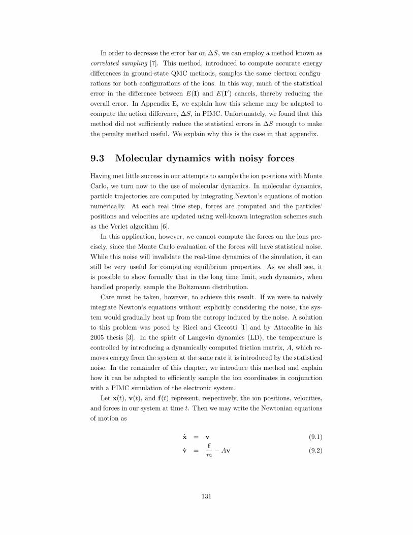
In order to decrease the error bar on ∆S, we can employ a method known as

correlated sampling [7]. This method, introduced to compute accurate energy

differences in ground-state QMC methods, samples the same electron configu-

rations for both configurations of the ions. In this way, much of the statistical

error in the difference between E(I) and E(I′) cancels, thereby reducing the

overall error. In Appendix E, we explain how this scheme may be adapted to

compute the action difference, ∆S, in PIMC. Unfortunately, we found that this

method did not sufficiently reduce the statistical errors in ∆S enough to make

the penalty method useful. We explain why this is the case in that appendix.

9.3 Molecular dynamics with noisy forces

Having met little success in our attempts to sample the ion positions with Monte

Carlo, we turn now to the use of molecular dynamics. In molecular dynamics,

particle trajectories are computed by integrating Newton’s equations of motion

numerically. At each real time step, forces are computed and the particles’

positions and velocities are updated using well-known integration schemes such

as the Verlet algorithm [6].

In this application, however, we cannot compute the forces on the ions pre-

cisely, since the Monte Carlo evaluation of the forces will have statistical noise.

While this noise will invalidate the real-time dynamics of the simulation, it can

still be very useful for computing equilibrium properties. As we shall see, it

is possible to show formally that in the long time limit, such dynamics, when

handled properly, sample the Boltzmann distribution.

Care must be taken, however, to achieve this result. If we were to naively

integrate Newton’s equations without explicitly considering the noise, the sys-

tem would gradually heat up from the entropy induced by the noise. A solution

to this problem was posed by Ricci and Ciccotti [1] and by Attacalite in his

2005 thesis [3]. In the spirit of Langevin dynamics (LD), the temperature is

controlled by introducing a dynamically computed friction matrix, A, which re-

moves energy from the system at the same rate it is introduced by the statistical

noise. In the remainder of this chapter, we introduce this method and explain

how it can be adapted to efficiently sample the ion coordinates in conjunction

with a PIMC simulation of the electronic system.

Let x(t), v(t), and f(t) represent, respectively, the ion positions, velocities,

and forces in our system at time t. Then we may write the Newtonian equations

of motion as

x = v (9.1)

v =f

m−Av (9.2)

131

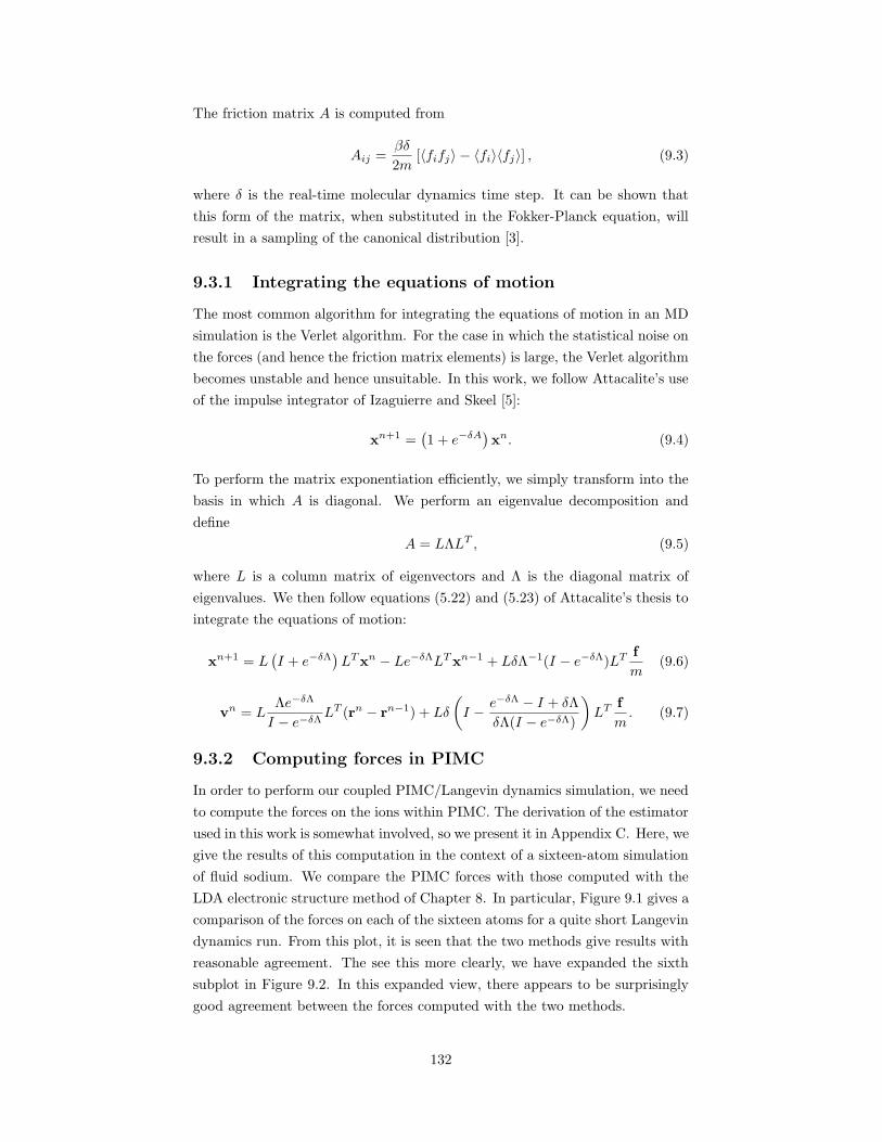
The friction matrix A is computed from

Aij =βδ

2m[〈fifj〉 − 〈fi〉〈fj〉] , (9.3)

where δ is the real-time molecular dynamics time step. It can be shown that

this form of the matrix, when substituted in the Fokker-Planck equation, will

result in a sampling of the canonical distribution [3].

9.3.1 Integrating the equations of motion

The most common algorithm for integrating the equations of motion in an MD

simulation is the Verlet algorithm. For the case in which the statistical noise on

the forces (and hence the friction matrix elements) is large, the Verlet algorithm

becomes unstable and hence unsuitable. In this work, we follow Attacalite’s use

of the impulse integrator of Izaguierre and Skeel [5]:

xn+1 =(1 + e−δA

)xn. (9.4)

To perform the matrix exponentiation efficiently, we simply transform into the

basis in which A is diagonal. We perform an eigenvalue decomposition and

define

A = LΛLT , (9.5)

where L is a column matrix of eigenvectors and Λ is the diagonal matrix of

eigenvalues. We then follow equations (5.22) and (5.23) of Attacalite’s thesis to

integrate the equations of motion:

xn+1 = L(I + e−δΛ

)LT xn − Le−δΛLT xn−1 + LδΛ−1(I − e−δΛ)LT f

m(9.6)

vn = LΛe−δΛ

I − e−δΛLT (rn − rn−1) + Lδ

(

I − e−δΛ − I + δΛ

δΛ(I − e−δΛ)

)

LT f

m. (9.7)

9.3.2 Computing forces in PIMC

In order to perform our coupled PIMC/Langevin dynamics simulation, we need

to compute the forces on the ions within PIMC. The derivation of the estimator

used in this work is somewhat involved, so we present it in Appendix C. Here, we

give the results of this computation in the context of a sixteen-atom simulation

of fluid sodium. We compare the PIMC forces with those computed with the

LDA electronic structure method of Chapter 8. In particular, Figure 9.1 gives a

comparison of the forces on each of the sixteen atoms for a quite short Langevin

dynamics run. From this plot, it is seen that the two methods give results with

reasonable agreement. The see this more clearly, we have expanded the sixth

subplot in Figure 9.2. In this expanded view, there appears to be surprisingly

good agreement between the forces computed with the two methods.

132

! #"%$'&

Figure 9.1: A comparison of the forces on the ions in a 16-atom Langevindynamics simulation of sodium. The x (blue), y (red), and z (black) componentsof the forces are computed with the PIMC estimator described in this chapter(solid lines) and within the Local Density Approximation (dashed lines). Theforces are given in Hartree/bohr.

(*)+( (*)+, (-) . (*)+/ (*)+0132 46587:9;=<

> (-):(-,

> (-):(-?

(*)+(*(

(-):(-?

(-):(-,

@ ABCDEFGBH BDDIJK AFBL

PSfrag replacements

Fx (PIMC)

Fx (LDA)

Fy (PIMC)

Fy (LDA)

Fz (PIMC)

Fz (LDA)

Figure 9.2: An expansion of sixth subplot of Figure 9.1. The magnified plotshows quite good agreement between the forces computed with PIMC and LDA.

133

9.3.3 Computing the covariance

In order to determine the appropriate drag coefficients, we need an accurate

estimate for the covariance matrix, C, whose elements are given by

Cij = 〈fifj〉 − 〈fi〉〈fj〉. (9.8)

Here, fi gives the ith component of the 3N -dimensional force vector. The av-

erage is taken over all PIMC samples since the last LD step. We also must

average over all k-points as described in Chapter 6.

Let us assume that we have forces from NMC PIMC steps for Nk k-points.

We may first average over all k-points, yielding NMC twist-averaged forces. We

can then compute the covariance of these samples using the normal variance

estimator. It is also important, however, to have an accurate estimate for the

autocorrelation time, κ. If successive PIMC samples of the force are correlated

with decay time, κ, this increases the flow rate of energy into the system by the

same factor.

9.3.4 Re-equilibration bias

After an LD update of the ion positions, the electron paths can no longer be

considered to be in an equilibrium configuration. Therefore it becomes necessary

to run a number of Monte Carlo steps to re-equilibrate. If done naively, many

steps may be required to return to (thermal) equilibrium, but if too few steps

are taken, a systematic bias on the forces can result in very unphysical behavior.

Because of inertia, the ions move in approximately the same direction each

Langevin time step. As a result, poorly equilibrated electrons tend to lag behind

the ions. Since the electron-ion interaction is attractive (except inside the core),

the electron paths create an artificial drag on the ions. This quickly leaches

kinetic energy from the ionic system and it cools rapidly. Within a few tens of

LD steps, the temperature can fall to a fraction of the desired temperature.

The artificial drag effect can be greatly reduced through the use of the space

warp method we described above. In Appendix G, it is shown that the method

was ineffective in our PIMC simulations, since the warping procedure gener-

ated large fluctuations of the kinetic action and Jacobian for the move, which

resulted in almost no ion moves being accepted. In the present context, how-

ever, we use the space warp method only to give a starting configuration for our

electron paths after each Langevin step for the ions. Since there is essentially

an independent PIMC simulation for each LD step, the space warp can be ap-

plied unconditionally, and thus the Jacobians for the transformation need not

be considered at all. This procedure drastically reduces the number of PIMC

simulation steps which are needed to equilibrate the the electrons to the new

ion positions.

134

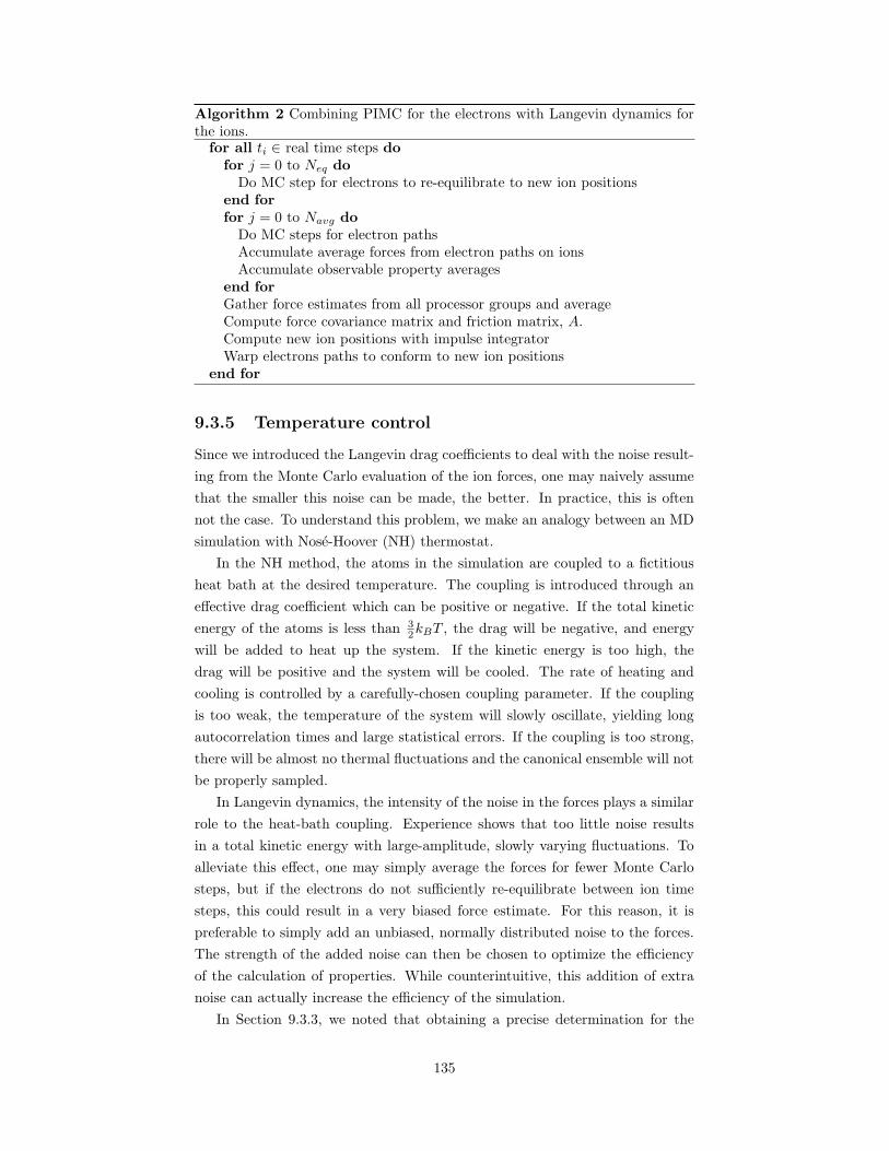
Algorithm 2 Combining PIMC for the electrons with Langevin dynamics forthe ions.

for all ti ∈ real time steps do

for j = 0 to Neq do

Do MC step for electrons to re-equilibrate to new ion positionsend for

for j = 0 to Navg do

Do MC steps for electron pathsAccumulate average forces from electron paths on ionsAccumulate observable property averages

end for

Gather force estimates from all processor groups and averageCompute force covariance matrix and friction matrix, A.Compute new ion positions with impulse integratorWarp electrons paths to conform to new ion positions

end for

9.3.5 Temperature control

Since we introduced the Langevin drag coefficients to deal with the noise result-

ing from the Monte Carlo evaluation of the ion forces, one may naively assume

that the smaller this noise can be made, the better. In practice, this is often

not the case. To understand this problem, we make an analogy between an MD

simulation with Nose-Hoover (NH) thermostat.

In the NH method, the atoms in the simulation are coupled to a fictitious

heat bath at the desired temperature. The coupling is introduced through an

effective drag coefficient which can be positive or negative. If the total kinetic

energy of the atoms is less than 32kBT , the drag will be negative, and energy

will be added to heat up the system. If the kinetic energy is too high, the

drag will be positive and the system will be cooled. The rate of heating and

cooling is controlled by a carefully-chosen coupling parameter. If the coupling

is too weak, the temperature of the system will slowly oscillate, yielding long

autocorrelation times and large statistical errors. If the coupling is too strong,

there will be almost no thermal fluctuations and the canonical ensemble will not

be properly sampled.

In Langevin dynamics, the intensity of the noise in the forces plays a similar

role to the heat-bath coupling. Experience shows that too little noise results

in a total kinetic energy with large-amplitude, slowly varying fluctuations. To

alleviate this effect, one may simply average the forces for fewer Monte Carlo

steps, but if the electrons do not sufficiently re-equilibrate between ion time

steps, this could result in a very biased force estimate. For this reason, it is

preferable to simply add an unbiased, normally distributed noise to the forces.

The strength of the added noise can then be chosen to optimize the efficiency

of the calculation of properties. While counterintuitive, this addition of extra

noise can actually increase the efficiency of the simulation.

In Section 9.3.3, we noted that obtaining a precise determination for the

135

covariance matrix of the forces can be difficult. In particular, with short PIMC

runs between each LD step, it may not be possible to accurately determine the

autocorrelation time, κ, of the forces. Autocorrelation of the forces in time

effectively increases the rate of energy input from the noise. As a result, it

often happens that the average temperature of the ions in the simulation is

higher than the desired one. In order to correct this problem, we introduce an

a posteriori scaling parameter, γ, which is multiplied to the friction matrix A.

Thus if we run the coupled simulation an discover the average ion temperature

was ten percent too high, we run the simulation again with a value of 1.1 for γ

. This latter simulation then typically has the correct average temperature. In

practice, we can explore large regions of the phase diagram with the same value

for γ.

9.4 Summary

In this chapter, we have discussed several possibilities for the sampling of the

classical ion configurations in our PIMC framework. The straight-forward ap-

proach of sampling the ions with Monte Carlo proved problematic, since large

changes in the fixed-phase action reduced the acceptance ratio for ion moves

to nearly zero. Two possible modifications to the Monte Carlo method were

proposed, both of which failed to completely solve the problem. As a result,

we resorted to a coupling of the PIMC simulation for the quantum electrons

to a Langevin dynamics simulation of the classical ions. We explained how the

method of Attacalite could be modified to work effectively with PIMC. In the

next, final chapter of this thesis, we will apply this method, and all the methods

we have described so far, to the simulation of fluid sodium near its liquid-vapor

critical point.

References

[1] Andrea Ricci and Giovanni Ciccotti. Algorithms for Brownian dynamics.

Molecular Physics, 101(12):1927, June 2003.

[2] Claudia Filippi and C.J. Umrigar. Correlated sampling in quantum Monte

Carlo: A route to forces. Phys. Rev. B., 61(24):R16291, 15 June 2000.

[3] Claudio Attacalite. RVB phase of hydrogen at high pressure: towards the

first ab-initio Molecular Dynamics by Quantum Monte Carlo. PhD thesis,

International School for Advanced Studies, Trieste, 24 October 2005.

[4] D.M. Ceperley and M. Dewing. The penalty method for random walks with

uncertain energies. J. Chem. Phys., 110(20):9812, 22 May 1999.

[5] J.A. Izagierre and R.D. Skeel. An impulse integrator for Langevin dynamics.

Mol. Phys., 100(24):3885, 2002.

136

[6] L. Verlet. Phys. Rev., 159:98, 1967.

[7] M. Dewing and D.M. Ceperley. Recent Advances in Quantum Monte Carlo

Methods, II, chapter Methods for Coupled Electronic-Ionic Monte Carlo.

World Scientific, 2002.

137

Chapter 10

Fluid sodium

The liquid-vapor transition of fluid metals forces one to search for

the unity in physical science. The existence of the liquid-vapor criti-

cal point makes possible a continuous transition from a dilute atomic

vapor to a dense metallic liquid. Thus a single set of experiments

on a single pure material takes one from the chemistry of reacting

molecular species to the domain of condensed matter physics. The

delicate mutual excitations of an atom pair in the vapor are a kind

of bashful invitation to the dance that leads ultimately to the col-

lective, electronic bacchanal known as the metallic state. It is the

essential challenge of this field to find the framework for

a unified theoretical description of this entire, continuous

process.

– Friedrich Hensel and William Warren, Jr. [6]

These words from two of the foremost experts in the field of fluid met-

als eloquently summarize both the allure and the challenge of understanding

the remarkable properties of these systems. The authors highlight the metal-

to-nonmetal (MNM) transition that occurs simultaneously with the transition

from the dense liquid to the atomic vapor. When crossing the first-order liquid-

vapor line, the MNM transition is discontinuous. This line has a terminus at

the liquid-vapor critical point, however. Thus, if a path in phase space is tra-

versed around the critical point, the system changes continuously from liquid to

vapor and metal to nonmetal. While such continuous MNM transitions occur in

other systems, they are usually driven by compositional changes, e.g. varying

the doping level in strongly-doped semiconductors, varying the metallic con-

centration in metal-ammonia solutions, etc. [15]. In contrast, pure fluid metals

provide a unique and interesting subject for study in that the MNM transition

is driven primarily by changes in the density. In this chapter, we present some

preliminary work in the simulation of fluid sodium with the methods developed

in this dissertation. We hope these methods can provide the unified framework

that Hensel and Warren are seeking.

138

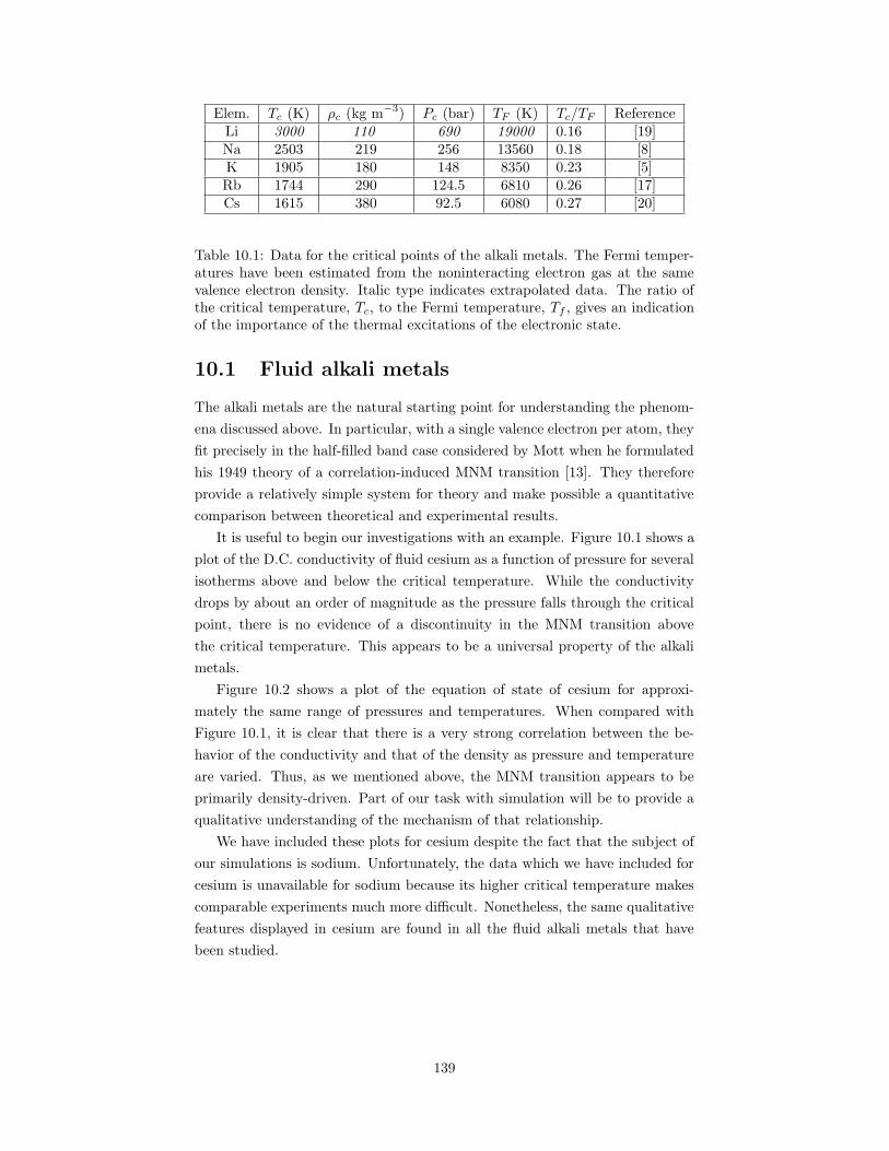
Elem. Tc (K) ρc (kg m−3) Pc (bar) TF (K) Tc/TF ReferenceLi 3000 110 690 19000 0.16 [19]Na 2503 219 256 13560 0.18 [8]K 1905 180 148 8350 0.23 [5]Rb 1744 290 124.5 6810 0.26 [17]Cs 1615 380 92.5 6080 0.27 [20]

Table 10.1: Data for the critical points of the alkali metals. The Fermi temper-atures have been estimated from the noninteracting electron gas at the samevalence electron density. Italic type indicates extrapolated data. The ratio ofthe critical temperature, Tc, to the Fermi temperature, Tf , gives an indicationof the importance of the thermal excitations of the electronic state.

10.1 Fluid alkali metals

The alkali metals are the natural starting point for understanding the phenom-

ena discussed above. In particular, with a single valence electron per atom, they

fit precisely in the half-filled band case considered by Mott when he formulated

his 1949 theory of a correlation-induced MNM transition [13]. They therefore

provide a relatively simple system for theory and make possible a quantitative

comparison between theoretical and experimental results.

It is useful to begin our investigations with an example. Figure 10.1 shows a

plot of the D.C. conductivity of fluid cesium as a function of pressure for several

isotherms above and below the critical temperature. While the conductivity

drops by about an order of magnitude as the pressure falls through the critical

point, there is no evidence of a discontinuity in the MNM transition above

the critical temperature. This appears to be a universal property of the alkali

metals.

Figure 10.2 shows a plot of the equation of state of cesium for approxi-

mately the same range of pressures and temperatures. When compared with

Figure 10.1, it is clear that there is a very strong correlation between the be-

havior of the conductivity and that of the density as pressure and temperature

are varied. Thus, as we mentioned above, the MNM transition appears to be

primarily density-driven. Part of our task with simulation will be to provide a

qualitative understanding of the mechanism of that relationship.

We have included these plots for cesium despite the fact that the subject of

our simulations is sodium. Unfortunately, the data which we have included for

cesium is unavailable for sodium because its higher critical temperature makes

comparable experiments much more difficult. Nonetheless, the same qualitative

features displayed in cesium are found in all the fluid alkali metals that have

been studied.

139

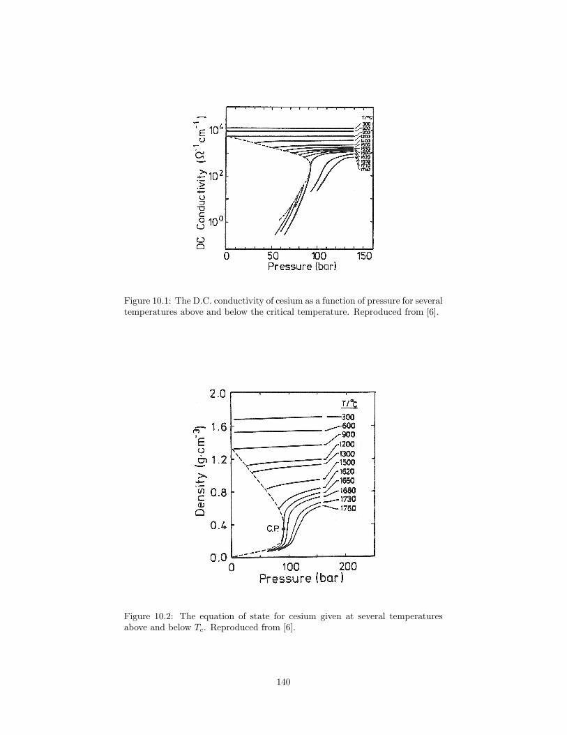
Figure 10.1: The D.C. conductivity of cesium as a function of pressure for severaltemperatures above and below the critical temperature. Reproduced from [6].

Figure 10.2: The equation of state for cesium given at several temperaturesabove and below Tc. Reproduced from [6].

140

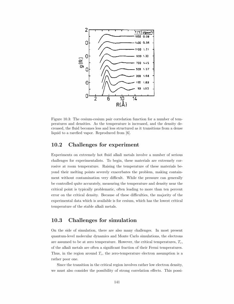
Figure 10.3: The cesium-cesium pair correlation function for a number of tem-peratures and densities. As the temperature is increased, and the density de-creased, the fluid becomes less and less structured as it transitions from a denseliquid to a rarefied vapor. Reproduced from [6].

10.2 Challenges for experiment

Experiments on extremely hot fluid alkali metals involve a number of serious

challenges for experimentalists. To begin, these materials are extremely cor-

rosive at room temperature. Raising the temperature of these materials be-

yond their melting points severely exacerbates the problem, making contain-

ment without contamination very difficult. While the pressure can generally

be controlled quite accurately, measuring the temperature and density near the

critical point is typically problematic, often leading to more than ten percent

error on the critical density. Because of these difficulties, the majority of the

experimental data which is available is for cesium, which has the lowest critical

temperature of the stable alkali metals.

10.3 Challenges for simulation

On the side of simulation, there are also many challenges. In most present

quantum-level molecular dynamics and Monte Carlo simulations, the electrons

are assumed to be at zero temperature. However, the critical temperatures, Tc,

of the alkali metals are often a significant fraction of their Fermi temperatures.

Thus, in the region around Tc, the zero-temperature electron assumption is a

rather poor one.

Since the transition in the critical region involves rather low electron density,

we must also consider the possibility of strong correlation effects. This possi-

141

!"

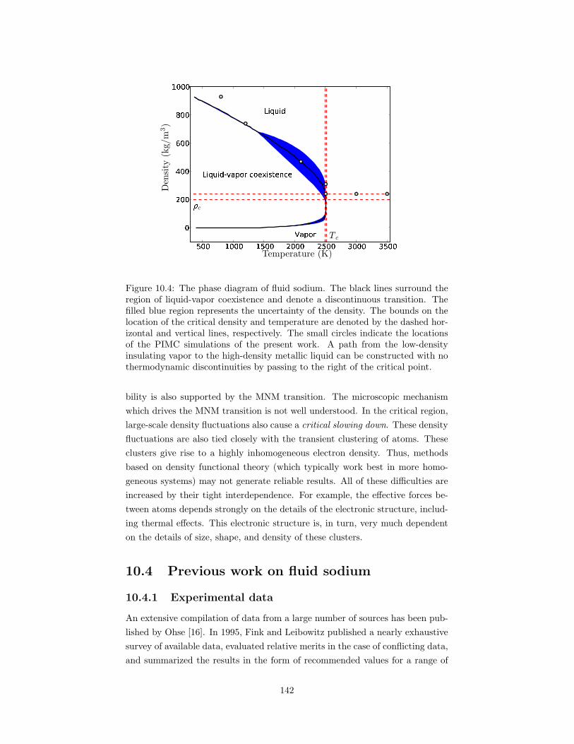
#$%cT

c&

PSfrag replacements

Temperature (K)

Den

sity

(kg/

m3)

Figure 10.4: The phase diagram of fluid sodium. The black lines surround theregion of liquid-vapor coexistence and denote a discontinuous transition. Thefilled blue region represents the uncertainty of the density. The bounds on thelocation of the critical density and temperature are denoted by the dashed hor-izontal and vertical lines, respectively. The small circles indicate the locationsof the PIMC simulations of the present work. A path from the low-densityinsulating vapor to the high-density metallic liquid can be constructed with nothermodynamic discontinuities by passing to the right of the critical point.

bility is also supported by the MNM transition. The microscopic mechanism

which drives the MNM transition is not well understood. In the critical region,

large-scale density fluctuations also cause a critical slowing down. These density

fluctuations are also tied closely with the transient clustering of atoms. These

clusters give rise to a highly inhomogeneous electron density. Thus, methods

based on density functional theory (which typically work best in more homo-

geneous systems) may not generate reliable results. All of these difficulties are

increased by their tight interdependence. For example, the effective forces be-

tween atoms depends strongly on the details of the electronic structure, includ-

ing thermal effects. This electronic structure is, in turn, very much dependent

on the details of size, shape, and density of these clusters.

10.4 Previous work on fluid sodium

10.4.1 Experimental data

An extensive compilation of data from a large number of sources has been pub-

lished by Ohse [16]. In 1995, Fink and Leibowitz published a nearly exhaustive

survey of available data, evaluated relative merits in the case of conflicting data,

and summarized the results in the form of recommended values for a range of

142

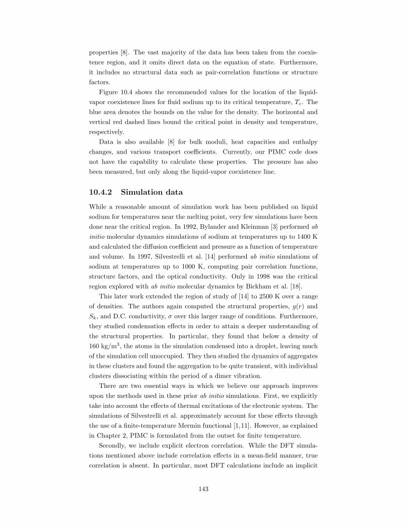
properties [8]. The vast majority of the data has been taken from the coexis-

tence region, and it omits direct data on the equation of state. Furthermore,

it includes no structural data such as pair-correlation functions or structure

factors.

Figure 10.4 shows the recommended values for the location of the liquid-

vapor coexistence lines for fluid sodium up to its critical temperature, Tc. The

blue area denotes the bounds on the value for the density. The horizontal and

vertical red dashed lines bound the critical point in density and temperature,

respectively.

Data is also available [8] for bulk moduli, heat capacities and enthalpy

changes, and various transport coefficients. Currently, our PIMC code does

not have the capability to calculate these properties. The pressure has also

been measured, but only along the liquid-vapor coexistence line.

10.4.2 Simulation data

While a reasonable amount of simulation work has been published on liquid

sodium for temperatures near the melting point, very few simulations have been

done near the critical region. In 1992, Bylander and Kleinman [3] performed ab

initio molecular dynamics simulations of sodium at temperatures up to 1400 K

and calculated the diffusion coefficient and pressure as a function of temperature

and volume. In 1997, Silvestrelli et al. [14] performed ab initio simulations of

sodium at temperatures up to 1000 K, computing pair correlation functions,

structure factors, and the optical conductivity. Only in 1998 was the critical

region explored with ab initio molecular dynamics by Bickham et al. [18].

This later work extended the region of study of [14] to 2500 K over a range

of densities. The authors again computed the structural properties, g(r) and

Sk, and D.C. conductivity, σ over this larger range of conditions. Furthermore,

they studied condensation effects in order to attain a deeper understanding of

the structural properties. In particular, they found that below a density of

160 kg/m3, the atoms in the simulation condensed into a droplet, leaving much

of the simulation cell unoccupied. They then studied the dynamics of aggregates

in these clusters and found the aggregation to be quite transient, with individual

clusters dissociating within the period of a dimer vibration.

There are two essential ways in which we believe our approach improves

upon the methods used in these prior ab initio simulations. First, we explicitly

take into account the effects of thermal excitations of the electronic system. The

simulations of Silvestrelli et al. approximately account for these effects through

the use of a finite-temperature Mermin functional [1,11]. However, as explained

in Chapter 2, PIMC is formulated from the outset for finite temperature.

Secondly, we include explicit electron correlation. While the DFT simula-

tions mentioned above include correlation effects in a mean-field manner, true

correlation is absent. In particular, most DFT calculations include an implicit

143

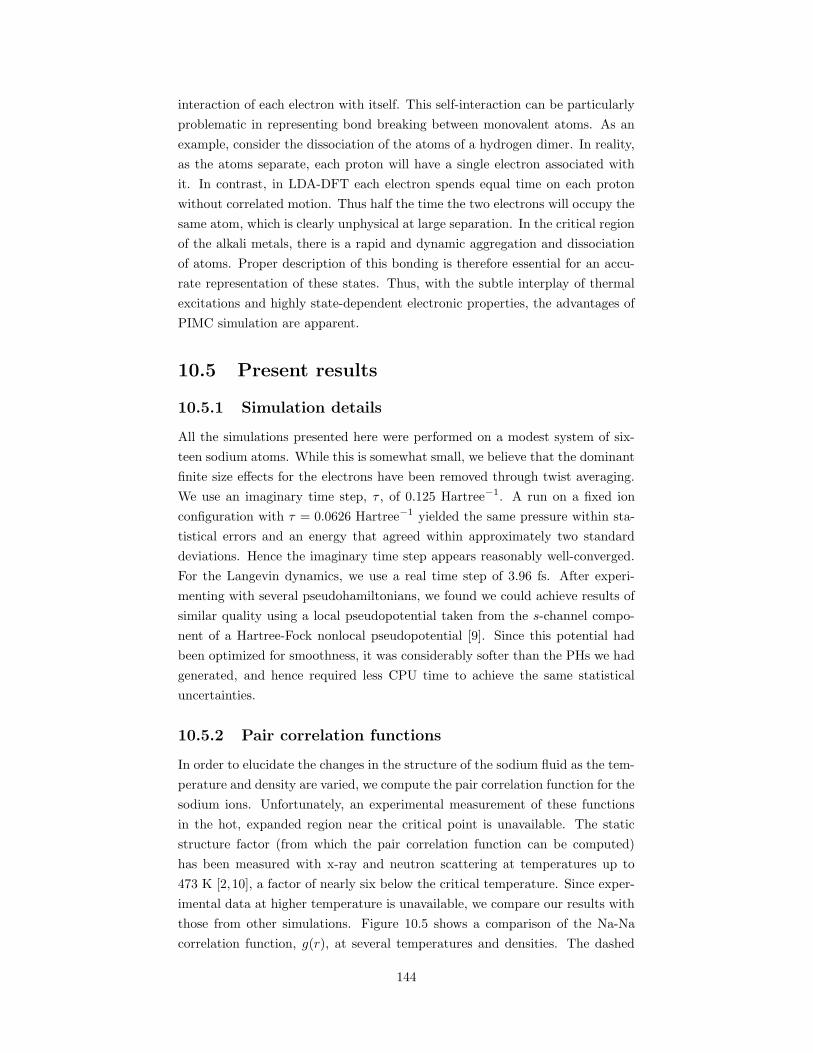
interaction of each electron with itself. This self-interaction can be particularly

problematic in representing bond breaking between monovalent atoms. As an

example, consider the dissociation of the atoms of a hydrogen dimer. In reality,

as the atoms separate, each proton will have a single electron associated with

it. In contrast, in LDA-DFT each electron spends equal time on each proton

without correlated motion. Thus half the time the two electrons will occupy the

same atom, which is clearly unphysical at large separation. In the critical region

of the alkali metals, there is a rapid and dynamic aggregation and dissociation

of atoms. Proper description of this bonding is therefore essential for an accu-

rate representation of these states. Thus, with the subtle interplay of thermal

excitations and highly state-dependent electronic properties, the advantages of

PIMC simulation are apparent.

10.5 Present results

10.5.1 Simulation details

All the simulations presented here were performed on a modest system of six-

teen sodium atoms. While this is somewhat small, we believe that the dominant

finite size effects for the electrons have been removed through twist averaging.

We use an imaginary time step, τ , of 0.125 Hartree−1. A run on a fixed ion

configuration with τ = 0.0626 Hartree−1 yielded the same pressure within sta-

tistical errors and an energy that agreed within approximately two standard

deviations. Hence the imaginary time step appears reasonably well-converged.

For the Langevin dynamics, we use a real time step of 3.96 fs. After experi-

menting with several pseudohamiltonians, we found we could achieve results of

similar quality using a local pseudopotential taken from the s-channel compo-

nent of a Hartree-Fock nonlocal pseudopotential [9]. Since this potential had

been optimized for smoothness, it was considerably softer than the PHs we had

generated, and hence required less CPU time to achieve the same statistical

uncertainties.

10.5.2 Pair correlation functions

In order to elucidate the changes in the structure of the sodium fluid as the tem-

perature and density are varied, we compute the pair correlation function for the

sodium ions. Unfortunately, an experimental measurement of these functions

in the hot, expanded region near the critical point is unavailable. The static

structure factor (from which the pair correlation function can be computed)

has been measured with x-ray and neutron scattering at temperatures up to

473 K [2,10], a factor of nearly six below the critical temperature. Since exper-

imental data at higher temperature is unavailable, we compare our results with

those from other simulations. Figure 10.5 shows a comparison of the Na-Na

correlation function, g(r), at several temperatures and densities. The dashed

144

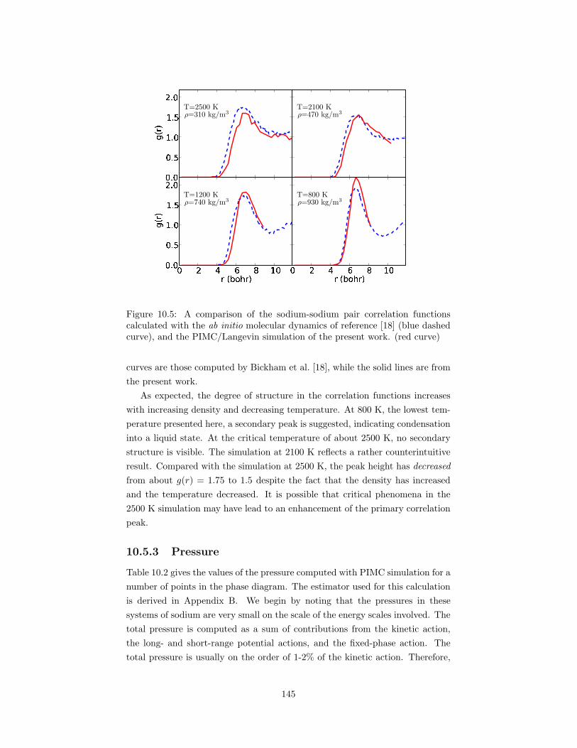
PSfrag replacements

ρ=310 kg/m3 ρ=470 kg/m3

ρ=740 kg/m3 ρ=930 kg/m3

T=2500 K T=2100 K

T=1200 K T=800 K

Figure 10.5: A comparison of the sodium-sodium pair correlation functionscalculated with the ab initio molecular dynamics of reference [18] (blue dashedcurve), and the PIMC/Langevin simulation of the present work. (red curve)

curves are those computed by Bickham et al. [18], while the solid lines are from

the present work.

As expected, the degree of structure in the correlation functions increases

with increasing density and decreasing temperature. At 800 K, the lowest tem-

perature presented here, a secondary peak is suggested, indicating condensation

into a liquid state. At the critical temperature of about 2500 K, no secondary

structure is visible. The simulation at 2100 K reflects a rather counterintuitive

result. Compared with the simulation at 2500 K, the peak height has decreased

from about g(r) = 1.75 to 1.5 despite the fact that the density has increased

and the temperature decreased. It is possible that critical phenomena in the

2500 K simulation may have lead to an enhancement of the primary correlation

peak.

10.5.3 Pressure

Table 10.2 gives the values of the pressure computed with PIMC simulation for a

number of points in the phase diagram. The estimator used for this calculation

is derived in Appendix B. We begin by noting that the pressures in these

systems of sodium are very small on the scale of the energy scales involved. The

total pressure is computed as a sum of contributions from the kinetic action,

the long- and short-range potential actions, and the fixed-phase action. The

total pressure is usually on the order of 1-2% of the kinetic action. Therefore,

145

Temperature (K) Density (kg/m3) Pressure (bar)3500 200 718 ± 702500 240∗ -132 ± 912500 240 -225 ± 913000 240 217 ± 863500 240 443 ± 832503 310 -980 ± 1401200 740 -3730 ± 330800 930 -7320 ± 676

Table 10.2: Pressures of fluid sodium computed with PIMC simulation for anumber of temperature/density phase points.

an accurate value for the total pressure requires that each of the individual

contributions be correct to within about 1%, making precise agreement with

experiment very challenging.

Furthermore, our experience shows that the pressure is quite sensitive to

the degree of equilibration of the system. All but one of the simulations in

Table 10.2 were initialized with a random ion configuration. We found, however,

that a significant fraction (∼30-40%) of the simulation needed to be discarded

because it had not yet equilibrated. In contrast, the simulation marked with

an * was initialized from a liquid configuration from a previous run. The value

of the pressure appeared to converge much sooner. These indications suggest

that longer runs should be attempted in the future to ensure equilibration has

been attained. Finally, we note that the rather unphysical negative pressures

obtained at high density most likely result from too sparse a k-point mesh. As

density increases, the bandwidth of the material increases, necessitating a more

dense mesh. All the pressure computations shown in Table 10.2 were computed

with a 2× 2× 2 mesh. While tests showed this mesh gave reasonable accuracy

at a density of 240 kg/m3, it is clearly insufficent at 930 kg/m3.

10.5.4 Qualitative observations concerning conductivity

Perhaps the most powerful aspect of simulation is not its ability to compute the

same properties which are measured in the laboratory, but rather to provide de-

tailed microscopic information which experiment usually cannot. In the present

fluid sodium system, the mechanisms which drive the continuous transition from

insulator to metal are not fully understood. Simulation can provide a unique

tool for developing insight into processes such as these. Here, we explain the

insight gained from our simulations.

In the finite-temperature Kubo formalism, the D.C. conductivity can be ex-

pressed in terms of a path integral over the electron velocity-velocity correlation

function (see Appendix B). In path integral Monte Carlo, paths which close on

a periodic image of their starting point are said to wind. It is these wind-

ing paths which contribute non-vanishing terms to the conductivity integral.

146

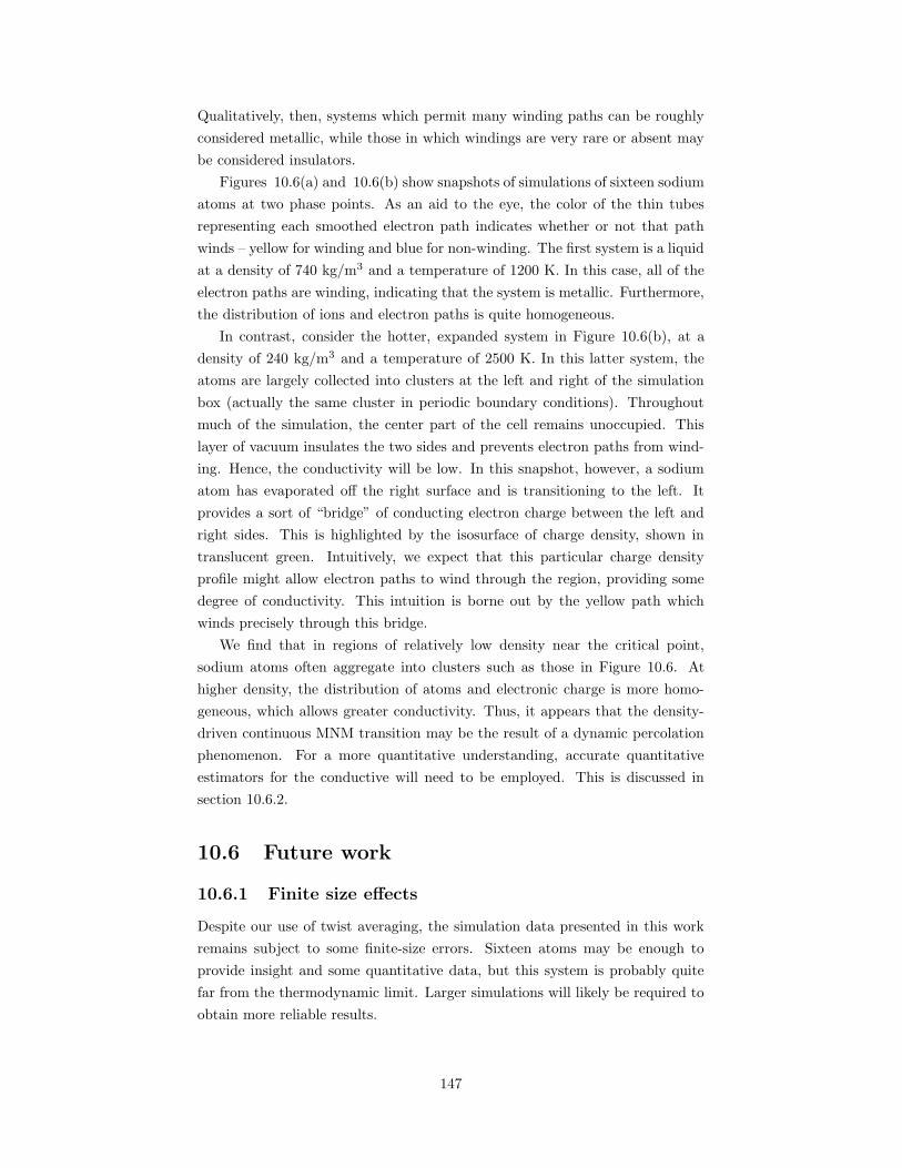
Qualitatively, then, systems which permit many winding paths can be roughly

considered metallic, while those in which windings are very rare or absent may

be considered insulators.

Figures 10.6(a) and 10.6(b) show snapshots of simulations of sixteen sodium

atoms at two phase points. As an aid to the eye, the color of the thin tubes

representing each smoothed electron path indicates whether or not that path

winds – yellow for winding and blue for non-winding. The first system is a liquid

at a density of 740 kg/m3 and a temperature of 1200 K. In this case, all of the

electron paths are winding, indicating that the system is metallic. Furthermore,

the distribution of ions and electron paths is quite homogeneous.

In contrast, consider the hotter, expanded system in Figure 10.6(b), at a

density of 240 kg/m3 and a temperature of 2500 K. In this latter system, the

atoms are largely collected into clusters at the left and right of the simulation

box (actually the same cluster in periodic boundary conditions). Throughout

much of the simulation, the center part of the cell remains unoccupied. This

layer of vacuum insulates the two sides and prevents electron paths from wind-

ing. Hence, the conductivity will be low. In this snapshot, however, a sodium

atom has evaporated off the right surface and is transitioning to the left. It

provides a sort of “bridge” of conducting electron charge between the left and

right sides. This is highlighted by the isosurface of charge density, shown in

translucent green. Intuitively, we expect that this particular charge density

profile might allow electron paths to wind through the region, providing some

degree of conductivity. This intuition is borne out by the yellow path which

winds precisely through this bridge.

We find that in regions of relatively low density near the critical point,

sodium atoms often aggregate into clusters such as those in Figure 10.6. At

higher density, the distribution of atoms and electronic charge is more homo-

geneous, which allows greater conductivity. Thus, it appears that the density-

driven continuous MNM transition may be the result of a dynamic percolation

phenomenon. For a more quantitative understanding, accurate quantitative

estimators for the conductive will need to be employed. This is discussed in

section 10.6.2.

10.6 Future work

10.6.1 Finite size effects

Despite our use of twist averaging, the simulation data presented in this work

remains subject to some finite-size errors. Sixteen atoms may be enough to

provide insight and some quantitative data, but this system is probably quite

far from the thermodynamic limit. Larger simulations will likely be required to

obtain more reliable results.

147

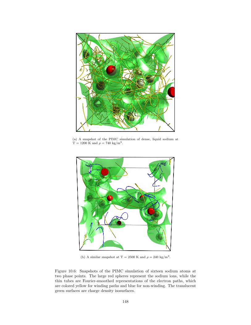
(a) A snapshot of the PIMC simulation of dense, liquid sodium atT = 1200 K and ρ = 740 kg/m3.

(b) A similar snapshot at T = 2500 K and ρ = 240 kg/m3.

Figure 10.6: Snapshots of the PIMC simulation of sixteen sodium atoms attwo phase points. The large red spheres represent the sodium ions, while thethin tubes are Fourier-smoothed representations of the electron paths, whichare colored yellow for winding paths and blue for non-winding. The translucentgreen surfaces are charge density isosurfaces.

148

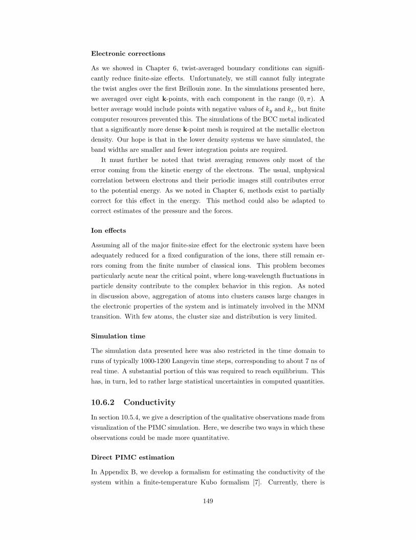
Electronic corrections

As we showed in Chapter 6, twist-averaged boundary conditions can signifi-

cantly reduce finite-size effects. Unfortunately, we still cannot fully integrate

the twist angles over the first Brillouin zone. In the simulations presented here,

we averaged over eight k-points, with each component in the range (0, π). A

better average would include points with negative values of ky and kz, but finite

computer resources prevented this. The simulations of the BCC metal indicated

that a significantly more dense k-point mesh is required at the metallic electron

density. Our hope is that in the lower density systems we have simulated, the

band widths are smaller and fewer integration points are required.

It must further be noted that twist averaging removes only most of the

error coming from the kinetic energy of the electrons. The usual, unphysical

correlation between electrons and their periodic images still contributes error

to the potential energy. As we noted in Chapter 6, methods exist to partially

correct for this effect in the energy. This method could also be adapted to

correct estimates of the pressure and the forces.

Ion effects

Assuming all of the major finite-size effect for the electronic system have been

adequately reduced for a fixed configuration of the ions, there still remain er-

rors coming from the finite number of classical ions. This problem becomes

particularly acute near the critical point, where long-wavelength fluctuations in

particle density contribute to the complex behavior in this region. As noted

in discussion above, aggregation of atoms into clusters causes large changes in

the electronic properties of the system and is intimately involved in the MNM

transition. With few atoms, the cluster size and distribution is very limited.

Simulation time

The simulation data presented here was also restricted in the time domain to

runs of typically 1000-1200 Langevin time steps, corresponding to about 7 ns of

real time. A substantial portion of this was required to reach equilibrium. This

has, in turn, led to rather large statistical uncertainties in computed quantities.

10.6.2 Conductivity

In section 10.5.4, we give a description of the qualitative observations made from

visualization of the PIMC simulation. Here, we describe two ways in which these

observations could be made more quantitative.

Direct PIMC estimation

In Appendix B, we develop a formalism for estimating the conductivity of the

system within a finite-temperature Kubo formalism [7]. Currently, there is

149

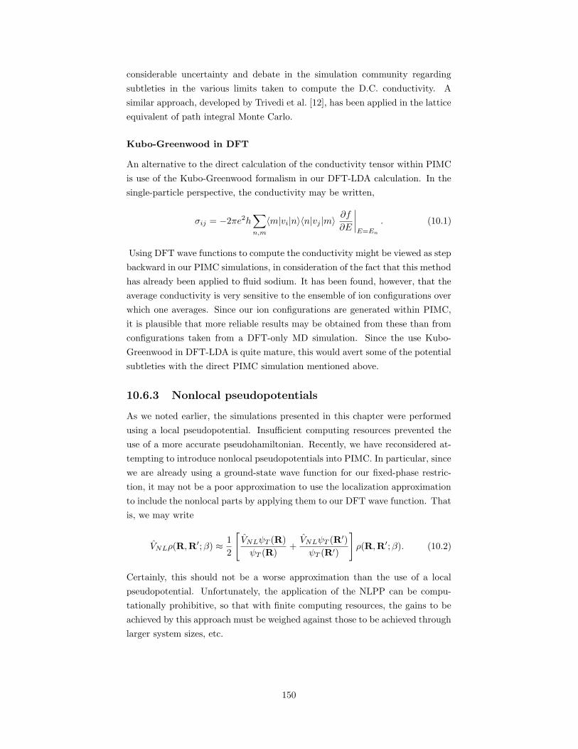
considerable uncertainty and debate in the simulation community regarding

subtleties in the various limits taken to compute the D.C. conductivity. A

similar approach, developed by Trivedi et al. [12], has been applied in the lattice

equivalent of path integral Monte Carlo.

Kubo-Greenwood in DFT

An alternative to the direct calculation of the conductivity tensor within PIMC

is use of the Kubo-Greenwood formalism in our DFT-LDA calculation. In the

single-particle perspective, the conductivity may be written,

σij = −2πe2h∑

n,m

〈m|vi|n〉〈n|vj |m〉∂f

∂E

∣∣∣∣E=En

. (10.1)

Using DFT wave functions to compute the conductivity might be viewed as step

backward in our PIMC simulations, in consideration of the fact that this method

has already been applied to fluid sodium. It has been found, however, that the

average conductivity is very sensitive to the ensemble of ion configurations over

which one averages. Since our ion configurations are generated within PIMC,

it is plausible that more reliable results may be obtained from these than from

configurations taken from a DFT-only MD simulation. Since the use Kubo-

Greenwood in DFT-LDA is quite mature, this would avert some of the potential

subtleties with the direct PIMC simulation mentioned above.

10.6.3 Nonlocal pseudopotentials

As we noted earlier, the simulations presented in this chapter were performed

using a local pseudopotential. Insufficient computing resources prevented the

use of a more accurate pseudohamiltonian. Recently, we have reconsidered at-

tempting to introduce nonlocal pseudopotentials into PIMC. In particular, since

we are already using a ground-state wave function for our fixed-phase restric-

tion, it may not be a poor approximation to use the localization approximation

to include the nonlocal parts by applying them to our DFT wave function. That

is, we may write

VNLρ(R,R′;β) ≈ 1

2

[

VNLψT (R)

ψT (R)+VNLψT (R′)

ψT (R′)

]

ρ(R,R′;β). (10.2)

Certainly, this should not be a worse approximation than the use of a local

pseudopotential. Unfortunately, the application of the NLPP can be compu-

tationally prohibitive, so that with finite computing resources, the gains to be

achieved by this approach must be weighed against those to be achieved through

larger system sizes, etc.

150

10.7 Summary and concluding remarks

This doctoral research project was originally motivated by the desire to extend

the range of applicability of the path integral Monte Carlo method to systems

containing elements heavier than hydrogen and helium. At the outset, it seemed

that a rather straightforward introduction of nonlocal pseudopotentials would

be possible. Discouraged by the lack of a finite-temperature equivalent of the

localization approximation used in diffusion Monte Carlo, we turned to the

use of pseudohamiltonians, which offered a mathematically well-defined way to

proceed. The computation of pair density matrices from PHs unfortunately

required the development of more complicated technology than that which was

needed for simple pair potentials.

The project grew in scope as Bryan Clark and I undertook the development

of a new, object-oriented simulation suite known as pimc++. This new suite

was designed from the beginning to become an extensible replacement for Ceper-

ley’s universal path integral (UPI) code [4]. More about this suite can be found

in Appendix A. The final goal of simulating a system containing heavy atoms

ultimately entailed developing new technology beyond the PHs. A modified

approach was required to appropriately handle the short/long-range breakups

for the PHs. The fixed-phase approach had to be adapted to work efficiently in

PIMC. Construction of a reasonable approximation for the trial phase entailed

the development of an embedded plane-wave DFT-LDA code designed to work

with pseudohamiltonians. Finally, in order to overcome the problems involved

with attempting to sample the ion configurations with Monte Carlo, a coupled

PIMC/Langevin simulation was developed. We believe that the methods devel-

oped here are not limited to the alkali metals, but can be applied to wide range

of systems in which electron correlation and thermal effects are important. We

hope that the release of the pimc++ code suite as free and open-source software

will speed the more widespread application of these methods and that through

them, new and interesting physical insight will gained.

References

[1] A. Alavi, J. Kohanoff, M. Parrinello, and D. Frenkel. Ab Initio Molecular

Dynamics with Excited Electrons. Phys. Rev. Lett., 73:2599, 7 November

1994.

[2] A.J. Greenfield, J. Wellendorf, and N. Wiser. X-Ray Determination of the

Static Structure Factor of Liquid Na and K. Phys. Rev. A, 4:1607, 1971.

[3] D. M. Bylander and Leonard Kleinman. Ab initio calculation of density

dependence of liquid-Na properties. Phys. Rev. B, 45(17), 1992.

[4] D.M. Ceperley. Path integrals in the theory of condensed helium. Rev.

Mod. Phys., 67(2):279, April 1995.

151

[5] F. Hensel, M. Stolz, G. Hohl, R. Winter, and W. Gotzlaff. J. Phys. IV

(Paris), Colloq. 1(C-5):191, 1991.

[6] Friedrich Hensel and William W. Warren Jr. Fluid Metals: The Liquid-

Vapor Transition of Metals. Princeton University Press, 1999.

[7] Gerald D. Mahan. Many-Particle Physics. Plenum Press, 1990.

[8] J. K. Fink and L. Leibowitz. THERMODYNAMIC AND TRANSPORT

PROPERTIES OF SODIUM LIQUID AND VAPOR. Technical Report

ANL/RE-95/2, Argonne National Laboratory, 9700 South Cass Avenue;

Argonne, Illinois 60439, January 1995.

[9] J. R. Trail and R. J. Needs. Smooth relativistic Hartree–Fock pseudopo-

tentials for H to Ba and Lu to Hg. J. Chem. Phys., 122:174109, 1 May

2005.

[10] M.J. Huijben and W. van der Lugt. X-ray and Neutron Diffraction from

Liquid Alkali Metals. Acta Cryst., A35:431–445, 1979.

[11] N. David Mermin. Thermal Properties of the Inhomogeneous Electron Gas.

Phys. Rev., 137(5A):A1441–A1443, March 1965.

[12] Nandini Trivedi, Richard T. Scalettar, and Mohit Randeria.

Superconductor-insulator transition in a disordered electronic system.

Phys. Rev. B, 54(6):3756, 1 August 1996.

[13] N.F. Mott. The Basis of the Electron Theory of Metals, with Special

Reference to the Transition Metals. Proc. Phys. Soc. London, 62:416, 1949.

[14] Pier Luigi Silvestrelli, Ali Alavi, and Michele Parrinello. Electrical-

conductivity calculation in ab initio simulations of metals: Application

to liquid sodium. Phys. Rev. B., 55(23):15515, 1997.

[15] P.P. Edwards and C.N.R. Rao. The Metallic and Nonmetallic States of

Matter. Taylor and Francis, London, 1985.

[16] R. W. Ohse. Handbook of Thermodynamic and Transport Properties of

Alkali Metals. Blackwell Scientific Publications, 1985.

[17] S. Jungst, B. Knuth, and F. Hensel. Phys. Rev. Lett., 55:2160, 1985.

[18] S.R. Bickham, O. Pfaffenzeller, L.A. Collins, J.D. Kress, and D. Hohl.

Ab initio molecular dynamics of expanded liquid sodium. Phys. Rev. B,

58(18):R11813, 1 November 1998.

[19] V.E. Fortov, A.N. Dremin, and A.A. Leontev. Teplofiz. Vys. Temp.

13(1072), 1975.

[20] W. Gotzlaff, G. Schonherr, and F. Hensel. Z. Phys. Chem. N.F., 156:219,

1988.

152

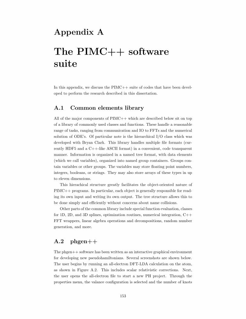
Appendix A

The PIMC++ softwaresuite

In this appendix, we discuss the PIMC++ suite of codes that have been devel-

oped to perform the research described in this dissertation.

A.1 Common elements library

All of the major components of PIMC++ which are described below sit on top

of a library of commonly used classes and functions. These handle a reasonable

range of tasks, ranging from communication and IO to FFTs and the numerical

solution of ODE’s. Of particular note is the hierarchical I/O class which was

developed with Bryan Clark. This library handles multiple file formats (cur-

rently HDF5 and a C++-like ASCII format) in a convenient, code transparent

manner. Information is organized in a named tree format, with data elements

(which we call variables), organized into named group containers. Groups con-

tain variables or other groups. The variables may store floating point numbers,

integers, booleans, or strings. They may also store arrays of these types in up

to eleven dimensions.

This hierachical structure greatly facilitates the object-oriented nature of

PIMC++ programs. In particular, each object is generally responsible for read-

ing its own input and writing its own output. The tree structure allows this to

be done simply and efficiently without concerns about name collisions.

Other parts of the common library include special function evaluation, classes

for 1D, 2D, and 3D splines, optimization routines, numerical integration, C++

FFT wrappers, linear algebra operations and decompositions, random number

generation, and more.

A.2 phgen++

The phgen++ software has been written as an interactive graphical environment

for developing new pseudohamiltonians. Several screenshots are shown below.

The user begins by running an all-electron DFT-LDA calculation on the atom,

as shown in Figure A.2. This includes scalar relativistic corrections. Next,

the user opens the all-electron file to start a new PH project. Through the

properties menu, the valance configuration is selected and the number of knots

153

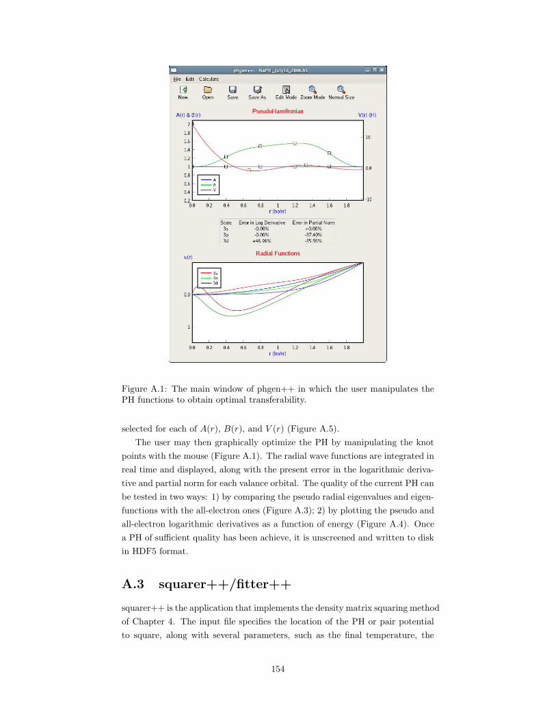
Figure A.1: The main window of phgen++ in which the user manipulates thePH functions to obtain optimal transferability.

selected for each of A(r), B(r), and V (r) (Figure A.5).

The user may then graphically optimize the PH by manipulating the knot

points with the mouse (Figure A.1). The radial wave functions are integrated in

real time and displayed, along with the present error in the logarithmic deriva-

tive and partial norm for each valance orbital. The quality of the current PH can

be tested in two ways: 1) by comparing the pseudo radial eigenvalues and eigen-

functions with the all-electron ones (Figure A.3); 2) by plotting the pseudo and

all-electron logarithmic derivatives as a function of energy (Figure A.4). Once

a PH of sufficient quality has been achieve, it is unscreened and written to disk

in HDF5 format.

A.3 squarer++/fitter++

squarer++ is the application that implements the density matrix squaring method

of Chapter 4. The input file specifies the location of the PH or pair potential

to square, along with several parameters, such as the final temperature, the

154

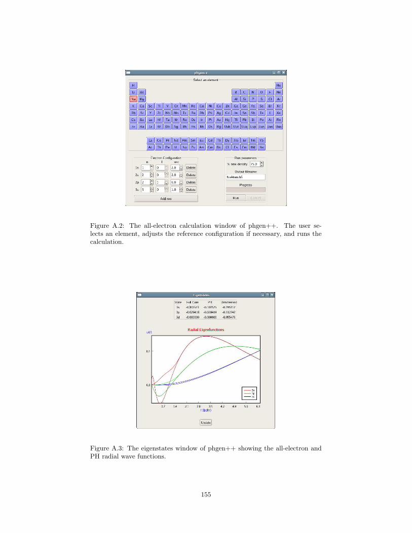
Figure A.2: The all-electron calculation window of phgen++. The user se-lects an element, adjusts the reference configuration if necessary, and runs thecalculation.

Figure A.3: The eigenstates window of phgen++ showing the all-electron andPH radial wave functions.

155

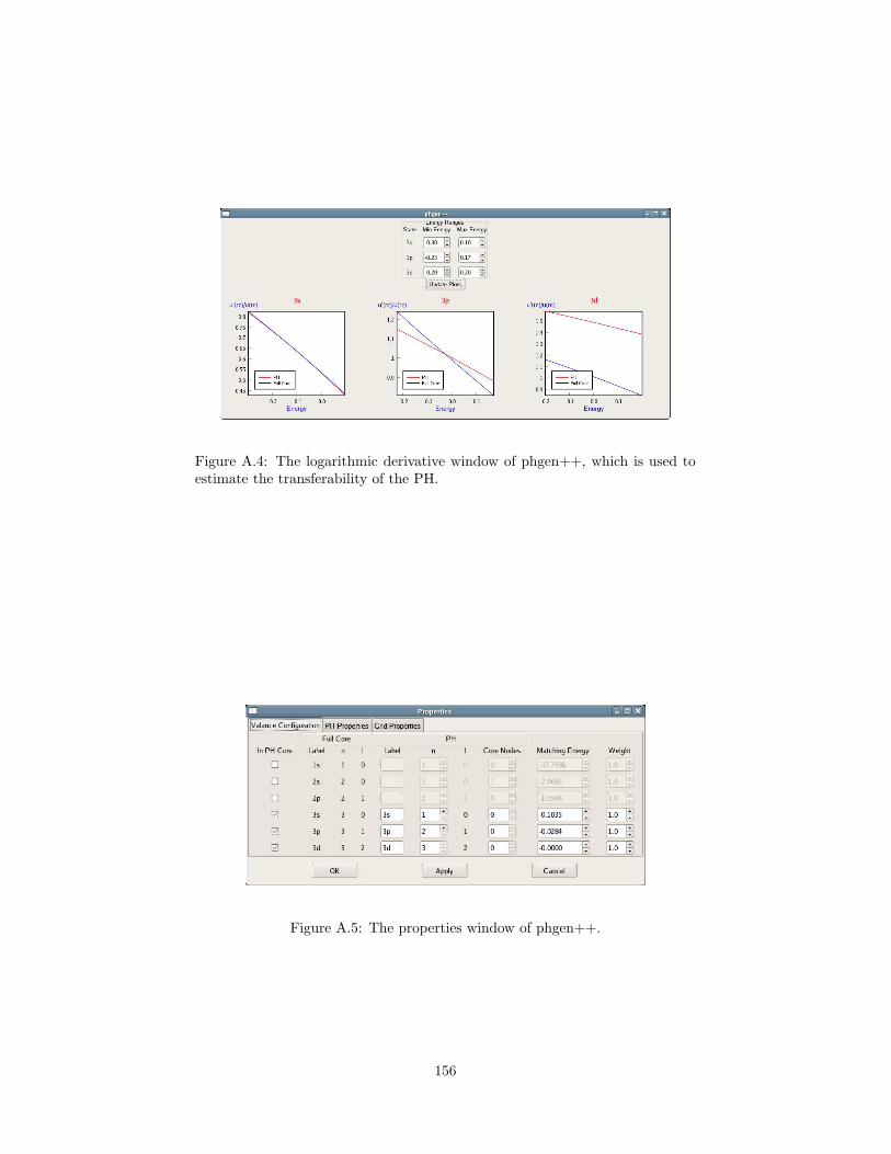
Figure A.4: The logarithmic derivative window of phgen++, which is used toestimate the transferability of the PH.

Figure A.5: The properties window of phgen++.

156

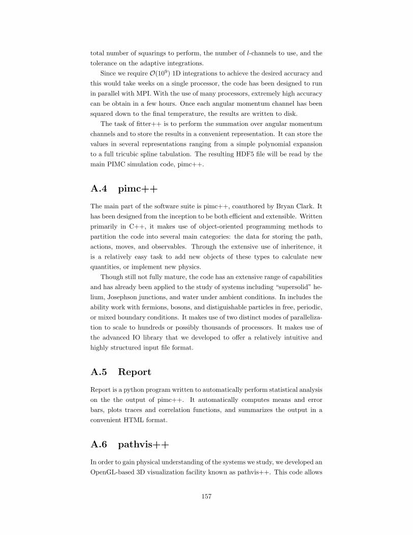
total number of squarings to perform, the number of l-channels to use, and the

tolerance on the adaptive integrations.

Since we require O(109) 1D integrations to achieve the desired accuracy and

this would take weeks on a single processor, the code has been designed to run

in parallel with MPI. With the use of many processors, extremely high accuracy

can be obtain in a few hours. Once each angular momentum channel has been

squared down to the final temperature, the results are written to disk.

The task of fitter++ is to perform the summation over angular momentum

channels and to store the results in a convenient representation. It can store the

values in several representations ranging from a simple polynomial expansion

to a full tricubic spline tabulation. The resulting HDF5 file will be read by the

main PIMC simulation code, pimc++.

A.4 pimc++

The main part of the software suite is pimc++, coauthored by Bryan Clark. It

has been designed from the inception to be both efficient and extensible. Written

primarily in C++, it makes use of object-oriented programming methods to

partition the code into several main categories: the data for storing the path,

actions, moves, and observables. Through the extensive use of inheritence, it

is a relatively easy task to add new objects of these types to calculate new

quantities, or implement new physics.

Though still not fully mature, the code has an extensive range of capabilities

and has already been applied to the study of systems including “supersolid” he-

lium, Josephson junctions, and water under ambient conditions. In includes the

ability work with fermions, bosons, and distiguishable particles in free, periodic,

or mixed boundary conditions. It makes use of two distinct modes of paralleliza-

tion to scale to hundreds or possibly thousands of processors. It makes use of

the advanced IO library that we developed to offer a relatively intuitive and

highly structured input file format.

A.5 Report

Report is a python program written to automatically perform statistical analysis

on the the output of pimc++. It automatically computes means and error

bars, plots traces and correlation functions, and summarizes the output in a

convenient HTML format.

A.6 pathvis++

In order to gain physical understanding of the systems we study, we developed an

OpenGL-based 3D visualization facility known as pathvis++. This code allows

157

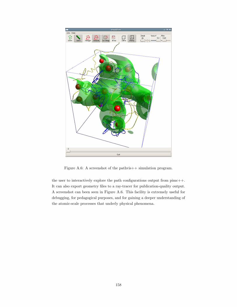
Figure A.6: A screenshot of the pathvis++ simulation program.

the user to interactively explore the path configurations output from pimc++.

It can also export geometry files to a ray-tracer for publication-quality output.

A screenshot can been seen in Figure A.6. This facility is extremely useful for

debugging, for pedagogical purposes, and for gaining a deeper understanding of

the atomic-scale processes that underly physical phenomena.

158

Appendix B

Computing observables

The end-products of our PIMC simulations are ultimately the observable aver-

ages which are computed during the simulation run. In this appendix, we give

a detailed description of how a number of useful observables may be computed.

We recall from Chapter 2 that diagonal observables may be computed in our

path integral simulation through

⟨

O⟩

≈ 1

N

N∑

j=1

O(Rji ,R

ji+1; τ), (B.1)

where

O(Ri,Ri+1; τ) ≡Oρ(Ri,Ri+1; τ)

ρ(Ri,Ri+1; τ). (B.2)

In this appendix, we derive explicit formulas for O(Ri,Ri+1; τ) for a number of

common properties of interest.

B.1 Energies

A number of distinct estimators for the average energy of the system have been

developed. In this work, we use the thermodynamic estimator,

〈H〉 = − 1

Z

∫

dR0Hρ(R0,R0;β)

ρ(R0,R0;β). (B.3)

In terms of our path integral simulation, we then write

〈H〉 = −⟨

1

M

M−1∑

i=0

Hρ(Ri,Ri+1; τ)

ρ(Ri,Ri+1; τ)S(Ri,Ri+1; τ)

⟩

PIMC

(B.4)

=

⟨

1

M

M−1∑

i=0

∂

∂τS(Ri,Ri+1; τ)

⟩

PIMC

, (B.5)

where we have made use of time-slice symmetry to average over the slices. Given

this expression, we must then compute the τ -derivative of each of our short-time

actions. As we noted in Chapter 4, we compute the τ -derivative of our pair

action simultaneously with its value through the matrix-squaring procedure.

159

The τ -derivative of the kinetic action, K, can be compute analytically as,

∂K(r, r′; τ)

∂τ=D

2τ− |r− r′|2

4λτ2, (B.6)

where D is the dimensionality of space. We recognize that the first term, which

comes from the normalization, contributes the classical kinetic energy, DkbT/2.

B.2 Pressure

In this section, we explain one way to estimate the pressure of a system of

interacting quantum particles in periodic boundary conditions. We recall that,

P = − dF

dΩ

∣∣∣∣β

, (B.7)

where F is the Helmholtz free energy and Ω is the volume of the simulation cell.

We now imagine scaling our cell by a factor ξ very near to one. Our coordinates

then undergo the replacement R→ sR. We may then write

P = − dF

dξ

dξ

dΩ

∣∣∣∣β,ξ=1

. (B.8)

Since dΩ/dξ = 3Ω, we then have

P = − 1

3Ω

dF

dξ

∣∣∣∣β,ξ=1

. (B.9)

We recall that F = − lnZ/β. Then

P =1

3ΩβZ

dZ

dξ

∣∣∣∣β,ξ=1

. (B.10)

Furthermore,

Z =

∫

d(sRi) e−S(ξRi) (B.11)

= ξ3NM

∫

dRie−S(ξRi). (B.12)

This leads to

P =1

3ΩβZ

[

3NMZ −∫

dRidSdξe−S

]

(B.13)

=

[

N

τΩ− 1

3Ωβ

⟨dSdξ

⟩

closed paths

]

. (B.14)

160

If we have time-slice symmetry, we recognize that S will be M times the action

for a single link. Then we have

P =1

3Ωτ

[

3N −⟨dSlink

dξ

⟩]

. (B.15)

B.2.1 Kinetic contribution

For the kinetic action, the spring term and the normalization factor will have

an ξ dependence.

Skinetic =3N

2ln

[4πλτ

ξ2

]

+ ξ2(R−R′)2/(4λτ). (B.16)

The ξ-derivative gives us then,

dSkinetic

dξ

∣∣∣∣ξ=1

= −3N +(R−R′)2

2λτ. (B.17)

B.2.2 Short-range contribution

The short-range action is written in terms the pair actions, defined in Chapter 4,

as

Sshort =∑

i<j

u(ξ(ri − rj), ξ(r′i − r′j); τ) (B.18)

=∑

i<j

u(ξq, ξz, ξs). (B.19)

Then, differentiating, we have

dSshort

ds

∣∣∣∣s=1

=∑

i<j

q∂u

∂qij+ z

∂u

∂zij+ s

∂u

∂sij. (B.20)

B.2.3 Long-range contribution

We note that the only terms which depend on the ion positions, R, are the ρk.

Let α represent the ion species. Then ρα is given by

ραk =

∑

j∈α

eiξk·Rj (B.21)

=∑

j∈α

eiξ(2πn/(ξL))·Rj . (B.22)

We note that the factors of ξ cancel from the above expression, reflecting the

fact that the ρk terms are simply sums over phase factors which depend on

coordinates in terms of dimensionless fractions of the box. Hence, they are

independent of the scale factor, ξ. However, we note that k is implicitly a

161

function of ξ, so that,

dSlong

dξ

∣∣∣∣ξ=1

=∑

α>β

[∑

k

Re(

ραkρ

β−k

) duαβk

dξ+NαNβ

(

duαβl0

dξ− duαβ

s0

dξ

)]

+1

2

∑

α

[∑

k

|ραk |2

duααk

dξ+ (Nα)

2

(duαα

l0

dξ− duαα

s0

dξ

)]

, (B.23)

where

duk

dξ=

∂uk

∂Ω

∂Ω

∂ξ+∂uk

∂k

dk

dξ(B.24)

= −3uk − k∂uk

∂k. (B.25)

B.2.4 Restricted-phase contribution

A final contribution to the pressure comes from the phase restriction we use to

approximately solve the fermion sign problem, as described in Chapter 7. This

phase action is of the form

Sphase =∑

i

λτ |∇iΦ(R)|2 (B.26)

dSphase

dξ

∣∣∣∣ξ=1

= 2λτ∑

i∈elecs

[∇iΦ(R)] · ddξ

[∇iΦ(R)] . (B.27)

If we assume that the wave function simply expands uniformly with the expand-

ing box, all our phases will remain constant as the scale factor ξ is changed.

However, the gradients of the phases will be proportional to 1/ξ. Hence, we

may writedSphase

dξ

∣∣∣∣ξ=1

= −2λτ∑

i∈elecs

|∇iΦ(R)|2 . (B.28)

B.3 Pair correlations functions

The pair-correlation function for two species, α and β, is given by [2]

g(r) =V

N2

⟨

δ(ri)∑

i∈α,j∈β,i6=j

δ(ri − rj)

⟩

. (B.29)

In practice, it is usual to reduce this to a function only of the magnitude of r.

We can then write g(r) in terms of g(r) as

g(r) =

∫

d3 r′δ(r − |r′|)g(r). (B.30)

In the context of our PIMC simulations, we can simply form a histogram of

the interparticle distances, |ri − rj |, in order to estimate g(r) for each pair of

162

particle species.

B.4 Conductivity

In general, computing time-dependent (or, equivalently, frequency-dependent)

properties is difficult within PIMC. In principle, frequency dependence can be

obtained through an inverse Laplace transform from imaginary-time correlation

functions, but because of statistical noise this transform is numerically poorly

conditioned. In the zero frequency limit, however, the inverse Laplace transform

becomes a simple integral in imaginary time. Thus, we may compute the static

limit of these time-dependent response functions straightforwardly.

Within the Kubo formalism, the DC conductivity, σαγ in the α direction

due to an applied field in the γ direction is given by [1]

Re(σαγ) =1

Ω

∫ ∞

0

dt e−st

∫ β

0

dβ′ Tr[

ρ jγ(−t− iβ′) jα]

. (B.31)

B.4.1 The j operator

The current operator, j, is given by

ji(β′) =

ie∇i

m. (B.32)

We apply this to the short time density matrix,

jαi (0)jγ

i (β′)ρ(R,R′; τ)

ρ(R,R′; τ)=

ie

m∇i ln [ρ(R,R′; τ)] (B.33)

= − iem∇iS(R,R′; τ), (B.34)

where the subscript i refers to the particle number. We recall that S has four

main contributions in our restricted phase formalism.

S = Skin + Sshort + Slong + Sphase (B.35)

Differentiating, we obtain

∇iSkinetic(R,R′; τ) =

∇i exp[−(ri − r′i)2/(4λτ)

]

exp [−(ri − r′i)2/(4λτ)](B.36)

=r′i − ri2λτ

, (B.37)

for the kinetic contribution and

∇iSshort(R,R′; τ) =

1

2∇i

∑

j 6=i

ushort(rj − ri, r′j − r′i; τ). (B.38)

163

for the short-range contribution. The long-range contribution can be calculated

as shown in the chapter on force calculations, in a manner similar to equa-

tion (C.26),

∇iSlong(R,R′; τ) = −2

∑

sgn(k)≥0

k Im(

eik·Rj

∑

σ

ρσ−ku

σiσk

)

, (B.39)

where σi is the species of the ith particle and the σ-summation is over all particle

types.

B.4.2 Discussion of contributing terms

Kinetic-kinetic term

The kinetic-kinetic correlation functions have the interesting property that they

provide a zero contribution unless paths wind around the simulation cell. Thus,

this part of the conductivity is essentially topological.

Kinetic-potential term

For winding paths, there is another contribution that comes from the cross terms

between the kinetic and potential actions. At each time slice, the electron-

electron terms sum to zero from Newton’s Third Law. Hence, these terms

reflect how much momentum is transferred from the electrons to the ions as they

scatter through the lattice. Since we have chosen to simulate ion classically, the

ion motion does not contribute to the conductivity. Given the mass disparity

between electrons and ions, this appears to be a reasonable approximation.

Potential-potential term

This term reflects the correlation between the net force on the electrons from

the ions at two different imaginary times. These terms will be of higher order

in τ than the above terms and should have a vanishing contribution in the limit

of small τ . In most cases, they can probably be neglected.

B.4.3 Using FFTs to compute convolutions

We need to compute the correlation function J ≡ 〈j(0)j(β)〉, which is evaluated

numerically as

J (n) =1

M

∑

i

j(i)j(i+ n), (B.40)

where j is periodic in its index. That is, j(M) = j(0). Since we wish to compute

the J (n) for all 0 ≤ n ≤M , it is most efficient to utilize fast Fourier transforms.

164

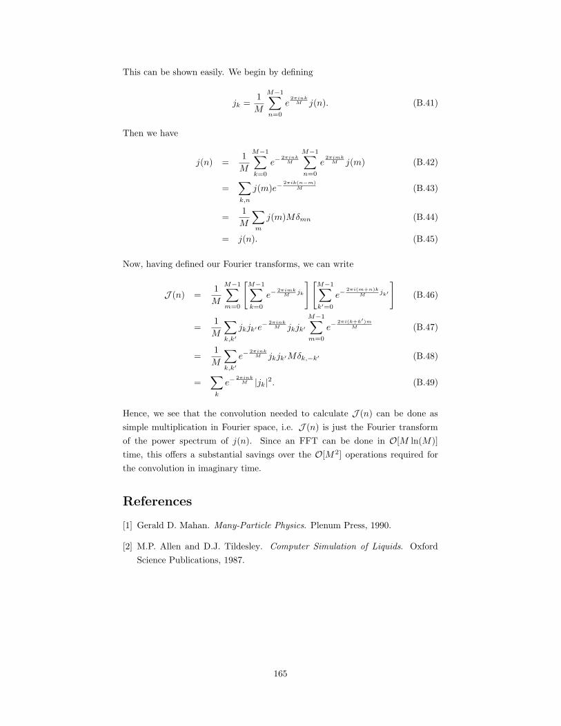
This can be shown easily. We begin by defining

jk =1

M

M−1∑

n=0

e2πink

M j(n). (B.41)

Then we have

j(n) =1

M

M−1∑

k=0

e−2πink

M

M−1∑

n=0

e2πimk

M j(m) (B.42)

=∑

k,n

j(m)e−2πik(n−m)

M (B.43)

=1

M

∑

m

j(m)Mδmn (B.44)

= j(n). (B.45)

Now, having defined our Fourier transforms, we can write

J (n) =1

M

M−1∑

m=0

[M−1∑

k=0

e−2πimk

Mjk

][M−1∑

k′=0

e−2πi(m+n)k

Mjk′

]

(B.46)

=1

M

∑

k,k′

jkjk′e−2πink

M jkjk′

M−1∑

m=0

e−2πi(k+k′)m

M (B.47)

=1

M

∑

k,k′

e−2πink

M jkjk′Mδk,−k′ (B.48)

=∑

k

e−2πink

M |jk|2. (B.49)

Hence, we see that the convolution needed to calculate J (n) can be done as

simple multiplication in Fourier space, i.e. J (n) is just the Fourier transform

of the power spectrum of j(n). Since an FFT can be done in O[M ln(M)]

time, this offers a substantial savings over the O[M 2] operations required for

the convolution in imaginary time.

References

[1] Gerald D. Mahan. Many-Particle Physics. Plenum Press, 1990.

[2] M.P. Allen and D.J. Tildesley. Computer Simulation of Liquids. Oxford

Science Publications, 1987.

165

Appendix C

Computing ion forces withPIMC

C.1 Introduction

In this chapter, we address the specifics of how thermal forces on classical ions

may be computed within the PIMC framework. We begin by recalling from

statistical mechanics that the average force exerted on particle i in the canonical

ensemble may be given by

Fi = −∇IiF , (C.1)

where F is the Helmholtz free energy. Then we may write

Fi =1

β∇Ii

lnZ (C.2)

= − 1

β〈∇Ii

S〉PIMC , (C.3)

where S denotes the total action, and the average is over all paths in the PIMC

simulation.

C.2 Kinetic action gradients

Clearly, the kinetic action of the electrons has no explicit dependence on the

location of the ions. Hence, the gradient of this term is identically zero.

C.3 Pair action gradients

Let us work in the relative coordinates given by

r ≡ relec − I (C.4)

r′ ≡ r′elec − I. (C.5)

166

Now u = u(r, r′; τ). We wish to compute the gradient, ∇Iu(r, r′; τ). Because of

symmetry, it is convenient to store, u(r, r′; τ) = u(q, s, z), where

q ≡ |r|+ |r′|

2, (C.6)

z ≡ |r| − |r′|

2, (C.7)

s ≡ |r− r′|. (C.8)

Since s is independent of I, we may write

∇Iu =∂u

∂q∇Iq +

∂u

∂z∇Iz. (C.9)

Then we may write

q =1

2

[(Rx − rx)2 + (Ry − ry)2 + (Rz − rz)2

] 12 +

[(Rx − r′x)2 + (Ry − r′y)2 + (Rz − r′z)2

] 12

(C.10)

z =[

(Rx − rx)2 + (Ry − ry)2 + (Rz − rz)2] 1

2 −[(Rx − r′x)2 + (Ry − r′y)2 + (Rz − r′z)2

] 12

. (C.11)

Hence,

∇Iq = − r + r′

2(C.12)

∇Iz = −[r− r′]. (C.13)

and finally we arrive at

∇Iu(q, z, s; τ) = −[1

2

∂u

∂q(r + r′)− ∂u

∂z(r− r′)

]

. (C.14)

C.3.1 Tricubic splines

A very general way to store the pair action, u(q, z, s; τ), is the use of tricubic

spline interpolation. This method tabulates the values of the action on a 3D

mesh, and uses piecewise tricubic interpolants constructed such that the value

and all first and second derivatives are continuous everywhere. The use of these

splines requires an box-shaped domain. Because of their definitions, the range

of z depends on q and the range of s depends on both q and z. Thus, we

must choose an alternate set of variables such that the spline has a box-shaped

167

domain in those variables. For reasons of accuracy, we choose,

q ≡ q (C.15)

y ≡ |z|zmax

(C.16)

t ≡ s− |z|zmax − |z|

, (C.17)

where

zmax = min [2q, z∗max(τ)] . (C.18)

z∗max(τ) is an appropriately chosen constant to reflect the range of z likely to

occur in PIMC simulation. On the rare occasion that z exceeds z∗max, we ex-

trapolate from the last point using derivative information from the spline.

Because zmax may depend on q, we must compute the partial derivatives of

u carefully.

∂u

∂q

∣∣∣∣z,s

=∂u

∂q

∣∣∣∣y,t

+∂u

∂y

∣∣∣∣q,t

∂y

∂q+∂u

∂t

∣∣∣∣q,y

∂t

∂q(C.19)

∂u

∂z

∣∣∣∣q,s

=∂u

∂q

∣∣∣∣y,t

0

∂q

∂z+∂u

∂y

∣∣∣∣q,t

∂y

∂z+∂u

∂t

∣∣∣∣q,y

∂t

∂z(C.20)

∂u

∂s

∣∣∣∣q,z

=∂u

∂q

∣∣∣∣y,t

0

∂q

∂s+∂u

∂y

∣∣∣∣q,t

∂y

∂s+∂u

∂t

∣∣∣∣q,y

∂t

∂s. (C.21)

C.4 Long-range forces

We recall the expressions for the long-range contribution to the action at a given

time slice,

Ulong =∑

α>β

[∑

k

Re(

ραkρ

β−k

)

uαβk −NαNβuαβ

s0 + Uk=0

]

(C.22)

+∑

α

[

−Nαuαα

l (0)

2+

1

2

∑

k

|ραk |2uαα

k −1

2(Nα)

2uαα

s0 + Uk=0

]

.

We note that the only terms which depend on the ion positions, I, are the ρk.

Let α represent the ion species. Then ρα is given by

ραk =

∑

j

eik·Ij (C.23)

∇Ijραk = ikeik·Ij . (C.24)

168

∇IjUlong = −

∑

k

k

Im(

eik·Ijρα−k

)

uααk +

∑

β 6=α

Im(

eik·Ijρβ−k

)

uαβk

= −∑

k

k∑

β

Im(

eik·Ijρβ−k

)

uαβk

= −∑

k

k Im

eik·Ij

∑

β

ρβ−ku

αβk

. (C.25)

C.4.1 Storage issues

We reduce our calculation of ραβk by noting that ραβ

−k =(

ραβk

)∗, and storing

only half of the k-vectors. Therefore, we need to compensate for this storage by

explicitly considering the vectors in (k,−k) pairs. We may then write

∇IjUlong = −

∑

sgn(k)≥0

kIm

eik·Ij

∑

β

ρβ−ku

αβk

− kIm

e−ik·Ij

∑

β

ρβku

αβk

= −2∑

sgn(k)≥0

k Im

eik·Ij

∑

β

ρβ−ku

αβk

(C.26)

C.5 Phase action

If, in our fixed-phase path integral formulation for fermions, our trial phases are

parameterized by the positions of the ionsIi, there must be a contribution to

the gradient of the action, ∇IiS, for a given instantaneous path in the simula-

tion. In this section, however, we argue that if our phase corresponds to that of

the exact density matrix, the net contribution to the force when averaged over

all paths will be zero. In practice, except for trivial problems, we never have an

exact specification of the phase. However, the approximation made in neglecting

the contribution due to an inexact phase is no worse than the approximation of

using the fixed-phase approach to begin with.

To begin our argument, we return to the partition function. The partition

function may be written as

Z =∑

s∈states

e−βEs . (C.27)

Then

Fi =1

βZ∇Ii

Z (C.28)

=1

βZ

∑

s

∇Iie−βEs (C.29)

=1

βZ

∑

s

〈ψs|∇IiV |ψs〉 e−βEs . (C.30)

169

The last is due to the Hellmann-Feynman theorem [1, 2]. Since ∇IiV is local,

the force can clearly be written in terms of an integral over the thermal electron

density. Thus, there must clearly be an estimator for Fi which does not have

an explicit dependence on the phase structure. This structure comes in only

in specifying the boundary conditions on the |ψs〉s that determine the charge

density. The estimator we have been using above is not the direct Hellmann-

Feynman estimator, but one based on pair actions. In the limit of τ → 0, the

arguments given here should still carry through.

References

[1] H. Hellman. Einfuhrung in die Quantumchemie, page 235. Deuticke, Leipzig,

1937.

[2] R.P. Feynman. Phys. Rev., 56:340, 1939.

170

Appendix D

Gradients of determinantwave functions

D.1 Posing the problem

Consider a wave function of the form

ψ(r0 . . . rN ) =

∣∣∣∣∣∣∣∣∣∣∣∣∣

φ0(r0) φ1(r0) φ2(r0) . . . φN (r0)

φ0(r1) φ1(r1) φ2(r1) . . . φ2(r1)

φ0(r2) φ1(r2) φ2(r2) . . . φ2(r2)...

......

. . ....

φ0(rN ) φ1(rN ) φ2(rN ) . . . φN (rN )

∣∣∣∣∣∣∣∣∣∣∣∣∣

≡ detA. (D.1)

Recall that in the Laplace expansion, a determinant can be written as a sum

over any row or column of the matrix element times its cofactor,

detA =∑

i

Aij(cof A)ij . (D.2)

In the Laplace expansion, the cofactor of a given element Aij is given by (−1)i+j

times the determinant of the matrix constructed by removing the ith row and

jth column from A. It is clear, then, that if we use the cofactor expansion along

the nth row, the cofactors will not depend on rn. This greatly simplifies the

gradient calculation since no chain rule will come in.

D.2 Solution

Unfortunately, the Laplace expansion, while illustrative, is computationally ex-

tremely costly. Fortunately, the reader may recall that the cofactor matrix can

be given by

cof A = det(A)(A−1

)T. (D.3)

The determinant may be computed by LU factorization in O(N 3) operations.

Let us then write the tensor formed by taking the gradients of the elements of

A,

Gij ≡ ∇φj(ri). (D.4)

171

Then, we can write

∇rjψ(r0 . . . rN ) =

∑

i

Gij(cof A)ij (D.5)

=∑

i

det(A) Gij

(A−1

)

ji(D.6)

Often, the quantity we require is ∇rjln(ψ), which is then given by

∇rjln [ψ(r0 . . . rN )] =

∑

i

Gij

(A−1

)

ji. (D.7)

These expressions are all that we require to implement our fixed-phase approach.

172

Appendix E

Correlated sampling foraction differences

E.1 Motivation

We wish to be able to accept or reject a proposed change to the ion configuration

by averaging over electron paths with the penalty method. In order to do this,

we need to be able to estimate the action difference between two configurations

of the ions, RA and RB , with the electronic degrees of freedom integrated out.

E.2 Sampling probability

It is, in general, impossible to select the optimal importance sampling function

without an a priori knowledge of the respective partition functions for the elec-

tronic system, Zelec(R) as a function of the ion positions. However, we can

select a nearly optimal importance function that has the desired properties. Let

SA and SB represent the imaginary time action for the systems with respective

ion positions RA and RB . Define

p∗ = e−SA + e−SB . (E.1)

Let us now consider the quantity we will use in determining whether to accept

or reject a change in the electron paths,

p∗new

p∗old=eSnew

A + eSnewB

eSoldA + eSold

B

. (E.2)

Now, consider splitting our paths over several processors, such that each pro-

cessor holds several time slices. In a usual PIMC simulation, most moves may

be made independently on each processor, since this acceptance ratio may be

factorized as a product of ratios calculated from the portion of the path on

each processor. Since we now have a sum of exponentials, we cannot make this

factorization, and hence the move cannot be exclusively “local” to a single pro-

cessor. We can, however, reduce the communication overhead that would be

incurred by doing a naive global move in which we have to perform a collective

sum over all processors at every stage of bisection.

173

In order to see how, let us then define new quantities,

S ≡ SA + SB

2(E.3)

∆S ≡ SA − SB

2. (E.4)

Then, we may rewrite

p∗ = e−S(e−∆S + e+∆S

). (E.5)

Consider now that the action SA may be given by summing over the actions,

SiA, from processors 1 through N .

SA =N∑

i=1

SiA, (E.6)

and similarly for SB . Then, our probability ratio may be written as

pnew∗pold∗

=exp

[

−∑Ni=1 S

newi

]

exp[

−∑Ni=1 S

oldi

]

exp

(

−∑Ni=1 ∆Snew

i

)

+ exp(

+∑N

i=1 ∆Snewi

)

exp(

−∑Ni=1 ∆Sold

i

)

+ exp(

+∑N

i=1 ∆Soldi

)

.

(E.7)

We first note that we have factored the acceptance ratio into two pieces, one

involving the S’s and one involving the ∆S’s. This factorization implies we can

separate those pieces into two acceptance stages – first accept or reject based

on the S’s. If we accept, we go on to accept or reject based on the ∆S’s.

Furthermore, we note that the S stage may be further factorized by processor:

exp[

−∑N

i=1 Snewi

]

exp[

−∑Ni=1 S

oldi

] =

N∏

i=1

exp[Sold

i − Snewi

]. (E.8)

This factorization implies that we may make the decision about whether to

accept the partial move on each processor independently.

Considered in the context of the multistage bisection move, each processor

begins at the highest bisection level. At each level, each processor may continue

to the next bisection level, or “opt out” of the collective move. Once we get to

the final bisection stage, we must do a collective communication, summing the

action changes on all the processors that have made it to this stage. Finally, we

accept or reject the move globally for all the processors simultaneously.

This scheme has the advantages that it avoid collective communication at

each stage. Furthermore, it prevents very unfavorable bisections (such as those

in which electrons overlap) from causing a global rejection of the move.

174

Algorithm 3 Modified correlated bisection algorithm.

for bisection level ← highest down to 0 do

Construct new path at this levelend for

Calculate new and old actions (excluding nodal) given by Si, where i is myprocessor number.Accept or reject local move based on Si

new − Siold.

if accepted local move then

δSiA ← (Si

A)new − (SiB)old (including nodal action)

δSiB = (Si

B)new − (SiB)old

else

δSiA ← 0

δSiB ← 0

end if

Perform global MPI sum on δSiA and δSi

B , yielding δSA and δSB .(SA)new ← (SA)old + δSA

(SB)new ← (SB)old + δSB

∆Snew ← 12 [(SA)new − (SB)new]

∆Sold ← 12 [(SA)old − (SB)old]

if accepted at level 1 then

Send my change in δS to collective sum.Accept or reject whole move globally based on collective sums.

else

Send 0 to collective sum for change in δS.end if

E.3 Difficulties

In the final analysis, correlated sampling works well only if the two probability

distributions being sampled have a sufficient amount of overlap. Unfortunately,

in the the case of the sodium simulations presented in this dissertation, this

was not the case. Correlated sampling did not reduce the statistical errors on

our action differeces sufficiently that the penalty method could be employed

efficiently. We hope that the considerations described here may serve as a

starting point for future investigations into this method.

175

Appendix F

Incomplete method:pair density matrices withthe Feynman-Kac formula

F.1 Introduction

In a Chapter 4, we discussed how to compute pair density matrices for an

electron interacting with a pseudohamiltonian core through the matrix squaring

method of Klemm and Storer [1]. Because of the numerical complexity involved,

it is very useful to have independent method to validate (or invalidate) the

results from that calculation. In this chapter, we discuss the computation of

the pair density matrix stochastically with the path-integral method of Feynman

and Kac.

We begin by defining the pseudohamilonian pair density matrix by

ρPH(r, r′;β) =⟨

r

∣∣∣e−βHPH

∣∣∣ r

′⟩

. (F.1)

Using the usual Trotter breakup, we can approximate this quantity with a dis-

crete path integral in imaginary time.

ρPH(r, r′;β) ≈∫

dr1 dr2 . . . drM ρ0(r, r1; τ) exp

−τ2[V (r) + V (r1)]

×ρ0(r1, r2; τ) exp

−τ2[V (r1) + V (r2)]

. . .

×ρ0(rM , r′; τ) exp

−τ2[V (rM ) + V (r′)]

,

(F.2)

where τ ≡ β/(M + 1). Define R ≡ r1, r2, . . . , rM. We break the integrand

into two quantities, defined as

P (R;β) ≡ ρ0(r, r1; τ)ρ0(r1, r2; τ) . . . ρ0(rM ; r′; τ) (F.3)

and

U(R;β) ≡ exp

−τ2

[V (r) + V (r′)] + τ

M∑

i=1

V (ri)

. (F.4)

Imagine we sample paths from the space of R with a sampling probablity density,

176

S(R). Then our integral can be written as a sum over N stochastic samples as

ρ(r, r′;β) ≈ 1

N

N∑

j=1

P (Rj ;β)

S(Rj)U(Rj ;β). (F.5)

In order to minimize the error of our stochastic average, we wish to have all the

terms in the sum be as close to each other as possible. This implies that we

wish to have the form for S(R) to be as close as possible to P (R;β)U(R;β) to

within a constant coefficient.

F.2 Sampling paths

We now address the question of how to sample paths. The free-particle density

matrix, ρ0(r, r′;β), is given by

(4πλβ)−D2 exp

[

− (r− r′)2

4λβ

]

, (F.6)

where λ = ~2

2m . We now describe how this expression can be used to sample a

free-particle path by a method know as the bisection algorithm.

F.2.1 The bisection algorithm

Given a segment starting at r at imaginary time 0 and ending at imaginary time

β, we need to know how to sample an intermediate point r′′ at imaginary time

β/2. For free particles, the proper probablity distribution is given by

P (r′′) = ρ(r, r′′;β/2)ρ(r′′, r′;β/2). (F.7)

That is, P (r′′) is the joint probability of a particle propagating from r to r′′ in

time β/2 and then from r′′ to r′ in time β/2. The product of two gaussians

is always a gaussian, so this quantity can be sampled exactly. Rearranging the

product, we obtain

exp

[

− (r1 − r)2

a1

]

exp

[

− (r− r2)2

a2

]

= exp

[

− (r1 − r2)2

a1 + a2

]

exp

[

−−(r− r)2

a

]

,

(F.8)

where

r =a1r2 + a2r1

a1 + a1(F.9)

a =

(1

a1+

1

a2

)−1

=a1a2

a1 + a2. (F.10)

Now that we know how to sample a single intermediate point, we can extend this

method to sample an arbitrarily detailed path between two points by recursively

applying single point sampling. That is, we begin by sampling a point, r0.5

177

between points r0 and r1. We then sample a point r0.25 between r0 and r0.5

and another point, r0.75 between r0.5 and r1. We can continue this process

indefinitely, but, in practice, only a certain number of levels are required for a

given accuracy.

In the case of a usual Hamiltonian, this function can be sampled exactly,

since it is a gaussian. Unfortunately, the position-dependent masses involved

in pseudohamiltonians imply that gassian sampling is only locally approximate.

Furthermore, the functional form must be generalized, since the radial and

tangential masses are not, in general, the same. For small β and |r− r′|, we can

approximate ρPH0 as

ρPH0 (r, r′;β) =

√

det(C)

π3exp [−(r− r′)C(r− r′)] , (F.11)

where C is a 3 × 3 matrix, which we now determine. Let U † be defined as a

3× 3 matrix whose rows are comprised of the unit vectors, r, θ, and φ.

U † ≡

r

θ

φ

. (F.12)

Also, define Q as

Q ≡

(2A(r)β)−1 0 0

0 (2B(r)β)−1 0

0 0 (2B(r)β)−1

, (F.13)

where A(r) and B(r) are the inverse radial and tangential masses, respectively.

The unit vectors can be computed using the following relations:

r =r

|r| (F.14)

φ =z × r

|z × r| (F.15)

θ = φ× r. (F.16)

Then C is given by

C = UQU †. (F.17)

Note that this form for ρPH0 (r, r′;β) is not symmetric in r and r′. If we chose

such a form, it would be a gaussian in neither r nor r′. The form we chose was to

be a perfect gaussian in r′. As we saw above, the quantity in which we are most

interested is actually the product ρPH0 (r, r′′;β/2)ρPH

0 (r′, r′′;β/2), which will be

perfectly symmetric in r and r′, and will be a perfect gaussian in r′′.

This form is still only locally approximate, but becomes exact in the limit

that τ → 0. To deal with this issue, we use a sufficent number of time slices to

178

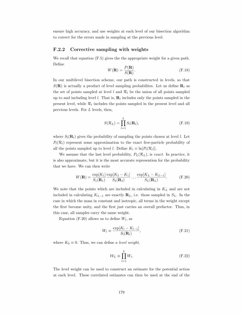
ensure high accuracy, and use weights at each level of our bisection algorithm

to correct for the errors made in sampling at the previous level.

F.2.2 Corrective sampling with weights

We recall that equation (F.5) gives the the appropriate weight for a given path.

Define

W (R) =P (R)

S(R). (F.18)

In our multilevel bisection scheme, our path is constructed in levels, so that

S(R) is actually a product of level sampling probabilites. Let us define Rl as

the set of points sampled at level l and Rl be the union of all points sampled

up to and including level l. That is, Rl includes only the points sampled in the

present level, while Rl includes the points sampled in the present level and all

previous levels. For L levels, then,

S(RL) =L∏

l=1

Sl(Rl), (F.19)

where Sl(Rl) gives the probability of sampling the points chosen at level l. Let

Pl(Rl) represent some approximation to the exact free-particle probability of

all the points sampled up to level l. Define Kl ≡ ln[Pl(Rl)].

We assume that the last level probability, PL(RL), is exact. In practice, it

is also approximate, but it is the most accurate represention for the probability

that we have. We can then write

W (R) =exp[K1]

S1(R1)

exp[K2 −K1]

S2(R2). . .

exp[KL −KL−1]

SL(RL). (F.20)

We note that the points which are included in calculating in KL and are not

included in calculating KL−1 are exactly RL, i.e. those sampled in SL. In the

case in which the mass in constant and isotropic, all terms in the weight except

the first become unity, and the first just carries an overall prefactor. Thus, in

this case, all samples carry the same weight.

Equation (F.20) allows us to define Wl, as

Wl ≡exp[Kl −Kl−1]

Sl(Rl), (F.21)

where K0 ≡ 0. Thus, we can define a level weight,

WL ≡L∏

l=1

Wl. (F.22)

The level weight can be used to construct an estimate for the potential action

at each level. These correlated estimates can then be used at the end of the

179

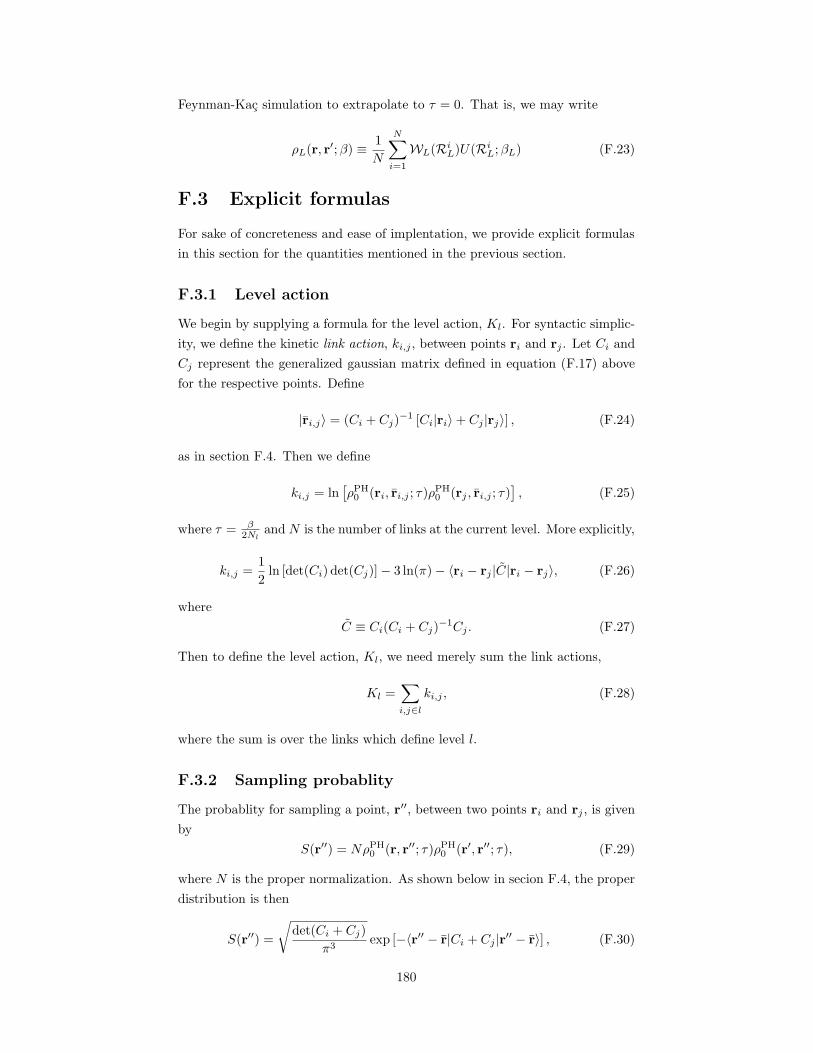
Feynman-Kac simulation to extrapolate to τ = 0. That is, we may write

ρL(r, r′;β) ≡ 1

N

N∑

i=1

WL(RiL)U(Ri

L;βL) (F.23)

F.3 Explicit formulas

For sake of concreteness and ease of implentation, we provide explicit formulas

in this section for the quantities mentioned in the previous section.

F.3.1 Level action

We begin by supplying a formula for the level action, Kl. For syntactic simplic-

ity, we define the kinetic link action, ki,j , between points ri and rj . Let Ci and

Cj represent the generalized gaussian matrix defined in equation (F.17) above

for the respective points. Define

|ri,j〉 = (Ci + Cj)−1 [Ci|ri〉+ Cj |rj〉] , (F.24)

as in section F.4. Then we define

ki,j = ln[ρPH0 (ri, ri,j ; τ)ρ

PH0 (rj , ri,j ; τ)

], (F.25)

where τ = β2Nl

and N is the number of links at the current level. More explicitly,

ki,j =1

2ln [det(Ci) det(Cj)]− 3 ln(π)− 〈ri − rj |C|ri − rj〉, (F.26)

where

C ≡ Ci(Ci + Cj)−1Cj . (F.27)

Then to define the level action, Kl, we need merely sum the link actions,

Kl =∑

i,j∈l

ki,j , (F.28)

where the sum is over the links which define level l.

F.3.2 Sampling probablity

The probablity for sampling a point, r′′, between two points ri and rj , is given

by

S(r′′) = NρPH0 (r, r′′; τ)ρPH

0 (r′, r′′; τ), (F.29)

where N is the proper normalization. As shown below in secion F.4, the proper

distribution is then

S(r′′) =

√

det(Ci + Cj)

π3exp [−〈r′′ − r|Ci + Cj |r′′ − r〉] , (F.30)

180

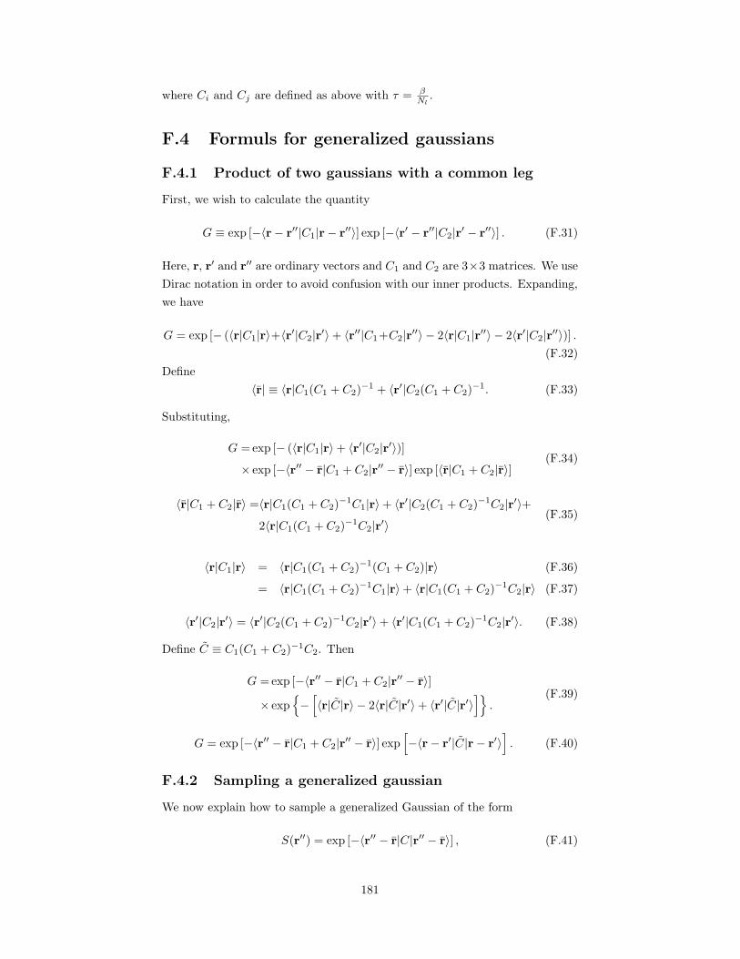
where Ci and Cj are defined as above with τ = βNl

.

F.4 Formuls for generalized gaussians

F.4.1 Product of two gaussians with a common leg

First, we wish to calculate the quantity

G ≡ exp [−〈r− r′′|C1|r− r′′〉] exp [−〈r′ − r′′|C2|r′ − r′′〉] . (F.31)

Here, r, r′ and r′′ are ordinary vectors and C1 and C2 are 3×3 matrices. We use

Dirac notation in order to avoid confusion with our inner products. Expanding,

we have

G = exp [− (〈r|C1|r〉+〈r′|C2|r′〉+ 〈r′′|C1+C2|r′′〉 − 2〈r|C1|r′′〉 − 2〈r′|C2|r′′〉)] .(F.32)

Define

〈r| ≡ 〈r|C1(C1 + C2)−1 + 〈r′|C2(C1 + C2)

−1. (F.33)

Substituting,

G = exp [− (〈r|C1|r〉+ 〈r′|C2|r′〉)]× exp [−〈r′′ − r|C1 + C2|r′′ − r〉] exp [〈r|C1 + C2|r〉]

(F.34)

〈r|C1 + C2|r〉 =〈r|C1(C1 + C2)−1C1|r〉+ 〈r′|C2(C1 + C2)

−1C2|r′〉+2〈r|C1(C1 + C2)

−1C2|r′〉(F.35)

〈r|C1|r〉 = 〈r|C1(C1 + C2)−1(C1 + C2)|r〉 (F.36)

= 〈r|C1(C1 + C2)−1C1|r〉+ 〈r|C1(C1 + C2)

−1C2|r〉 (F.37)

〈r′|C2|r′〉 = 〈r′|C2(C1 + C2)−1C2|r′〉+ 〈r′|C1(C1 + C2)

−1C2|r′〉. (F.38)

Define C ≡ C1(C1 + C2)−1C2. Then

G = exp [−〈r′′ − r|C1 + C2|r′′ − r〉]

× exp

−[

〈r|C|r〉 − 2〈r|C|r′〉+ 〈r′|C|r′〉]

.(F.39)

G = exp [−〈r′′ − r|C1 + C2|r′′ − r〉] exp[

−〈r− r′|C|r− r′〉]

. (F.40)

F.4.2 Sampling a generalized gaussian

We now explain how to sample a generalized Gaussian of the form

S(r′′) = exp [−〈r′′ − r|C|r′′ − r〉] , (F.41)

181

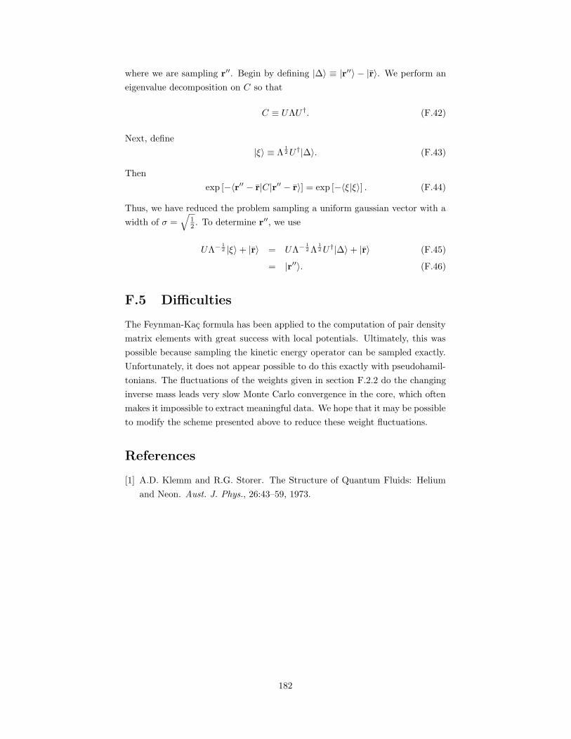
where we are sampling r′′. Begin by defining |∆〉 ≡ |r′′〉 − |r〉. We perform an

eigenvalue decomposition on C so that

C ≡ UΛU †. (F.42)

Next, define

|ξ〉 ≡ Λ12U †|∆〉. (F.43)

Then

exp [−〈r′′ − r|C|r′′ − r〉] = exp [−〈ξ|ξ〉] . (F.44)

Thus, we have reduced the problem sampling a uniform gaussian vector with a

width of σ =√

12 . To determine r′′, we use

UΛ− 12 |ξ〉+ |r〉 = UΛ− 1

2 Λ12U †|∆〉+ |r〉 (F.45)

= |r′′〉. (F.46)

F.5 Difficulties

The Feynman-Kac formula has been applied to the computation of pair density

matrix elements with great success with local potentials. Ultimately, this was

possible because sampling the kinetic energy operator can be sampled exactly.

Unfortunately, it does not appear possible to do this exactly with pseudohamil-

tonians. The fluctuations of the weights given in section F.2.2 do the changing

inverse mass leads very slow Monte Carlo convergence in the core, which often

makes it impossible to extract meaningful data. We hope that it may be possible

to modify the scheme presented above to reduce these weight fluctuations.

References

[1] A.D. Klemm and R.G. Storer. The Structure of Quantum Fluids: Helium

and Neon. Aust. J. Phys., 26:43–59, 1973.

182

Appendix G

Incomplete method: spacewarp for PIMC

In our PIMC simulation, we have quantum electron paths and classical ions.

We would like to update the ions with a Monte Carlo move. When we do so,

however, the action of the system changes at every time slice, since the ion

positions are identical at every time slice. In addition, the restricted-phase

action is updated everywhere since the wave functions depend parametrically

on the ion positions. If the phase restriction changes significantly, the ion move

is almost always rejected. The puts severe limitations on the distance the ions

may be moved in each step and strongly inhibits efficiency. In fact, we find that

for attempted moves larger than 0.05 bohr, the move is almost always rejected.

A possible solution may be adapted from ground state calculations. The

space-warp [1] tranformation of Filippi and Umrigar was introduced in order

to facilitate the correlated sampling of systems with two different ion configu-

rations. This appendix details our attempt to adapt this method to work in

PIMC. Unfortunately, the approach we took neglected a subtle contribution to

the Jacobian for the transformation, making the approach unusable. We have

nonetheless included this appendix in the hope that it may be a useful starting

point for investigations in the future.

G.1 The original transformation

The space-warp is a continuous spatial traformation function that effectively

translates electrons along with the nearest ions. In particular, let r and I

represent electron and ion positions, respectively. If we propose an ion move

I→ I + ∆I, the warp function is given by

w(ri) = ri +∑

j

ωij∆Ij , (G.1)

where the ωij is a weight function normalized such that∑

j ωij = 1. The

normalization can be included explicitly by writing

ωij =φ(|ri − Ij |)

∑

j φ(|ri − Ij |). (G.2)

183

The most common choice in the literature for the weight function has been,

φ(r) = r−4. The electron subscripts are not needed for the following discussion,

so they are omitted from this point forward.

G.1.1 The Jacobian

In Metropolis Monte Carlo, we must compute the ratios of the reverse and

forward transition probablity densities for each move. Since the space warp

transformation expands space in some regions and shrinks it in others, this

ratio will not, in general, be unity. In particlar, it will be the ratio of the

Jacobians for the reverse and forward transformations. Here, we compute that

Jacobian.

Since each electron is warped independently, the Jacobian for the entire move

can be written as a product of the Jacobians for each electron. Thus, we write

the Jacobian matrix for warping a single electron at a single time slice as

J =∂w(r)

∂r, (G.3)

The Jacobian itself is the determinant of this 3× 3 tensor of partial derivatives.

The matrix can be written as

Jαβ = δα,β +∑

i

(∆i)α

∂ωi

∂rβ. (G.4)

The partial derivative may, in turn, be expressed as

∂ωi

∂r= ωi

g(di)ri −∑

j

ωjg(dj)rj

, (G.5)

where dj = |r− Ij |, g(r) = ddr lnφ(ξ)

∣∣ξ=r

, and r = (r− Ij)/dj .

G.1.2 The reverse space warp

In order to obey detailed balance in Monte Carlo, we must have a move which

reverses a given move. Thus, we require the ability to reverse the space warp

transformation. That is, given a vector r′, we must find r such that w(r) = r′.

Since the warp transformation is a nonlinear function of the ion positions, it is

not, in general, possible to compute the reverse warp analytically. We show here,

however, that it is a simple matter to solve for r numerically, using Newton’s

method.

We begin by defining rn as the guess for r in the nth iteration of our search.

We linearize the warp transformation about rn as

w(rn+1) ≈ w(rn) + Jn(rn+1 − rn) (G.6)

184

We then set the RHS of the above equation to r′ and solve for rn+1, yielding

rn+1 = rn + (Jn)−1 [r′ −w(rn)] . (G.7)

To complete the algorithm, we need only to specify the initial guess for r0. For

simplicity we choose r0 = r′. This process typically converges within three to

four iterations to machine precision. The Jacobian for the reverse move can

then be given by

J rev(r′) = [J(r)]−1. (G.8)

G.2 Difficulties with PIMC

There are several difficulties which prevent a naive application of the space

warp method in PIMC. The problems stem essentially from the extremely high-

dimensional nature of the electron paths. A typical simulation involving elec-

trons may have ∼ 103 time slices. Any problem which may decrease the accep-

tance ratio even by a small fraction at each slice will have catastrophic effects

when considering a thousand slices moving together.

An essential property of the space warp is that is contracts and/or expands

space, depending on the proposed change in ion positions. This has two major

effects in our simulation. First, we must account for this expansion or contrac-

tion explicitly in our acceptance criteria in the form of the ratio of the transition

probability density. Since the warp is deterministic, the probability of proposing

the forward and reverse moves are equal, given the same initial configuration.

If we recall that we must consider the ratio of probability densities, however,

we find that

Trev. warp

Tforw. warp=

1/dΩrev.

1/dΩforw.=dΩforw.

dΩrev.= det Jforw., (G.9)

where dΩ represents a differential volume element. Most often, for small dis-

placements of the ions, at each time slice, this Jacobian is within a few percent of

unity, but when raised to the thousandth power, it becomes, in practical terms,

essentially zero or infinity. In the following discussion, I will refer to both the

Jacobian matrix and its determinant as simply the Jacobian – which is meant

at any given point is obvious from the context.

Secondly, the warp by its nature stretches or contracts the links on the paths,

and, as a result, changes the kinetic action. Because all links are potentially

affected, the change in kinetic action can be significant. The two contributions

to the acceptance probability, the Jacobians for the warp and the change in

kinetic action, usually enter with opposite sign. That is, when the logarithm of

the Jacobian is positive, the change in kinetic action will generally be negative,

but the two terms do not cancel in detail. This results in a wildly fluctuating

acceptance probability, which makes the naive algorithm impractical.

185

G.3 The PIMC space warp

To overcome these difficulties, we wish to construct a move which tries to satify

the following criteria:

• The move roughly tracks the conventional space warp of Filippi and Um-

rigar, but not precisely.

• The move is such that the ratio of the reverse and forward Jacobians for

the move precisely cancels the change in kinetic action. As a consequence

moves of noninteracting electrons would always be accepted.

• The reverse move must be possible (preferably easy) to construct so that

we obey detailed balance.

In this appendix, we describe a PIMC space warp (PSW) move that satisfies

these criteria. From this point, the term space warp refers to the single-particle

warping procedure and PSW refers to the aggregate move consisting of ion move

and warping of all electron paths. Simply stated, the algorthm for the PSW

move is:

1. Choose a translation for each ion from a gaussian distrubution with a

specified width

2. Perform a forward space warp on each electron at the even time slices.

3. Use the similar triangle construction given below to warp the odd slices

to be commensurate with the even slices.

4. Apply the tranverse path scaling on the odd slices to set the kinetic energy

change to compensate for the Jacobians.

5. Accept or reject the aggregate move based on the change in the total

action.

G.3.1 The ion displace step

The move begins by choosing a random displacement for the ions. For simplicity,

we choose displacing each by a normally distributed random variate of width σ,

which is chosen to maximize the diffusion efficiency. In practice, for the 16-atom

sodium systems studied in this work, a typical value is σ = 0.3 bohr.

One may also consider a more sophisticated move for the ions, such as force

bias Monte Carlo. In this approach, the gaussian for the displacement is not

centered on the present position, but is displaced from the present position by

some distance in the direction of the force on the ions. In the case of this

work, computing the PIMC forces at each step would be expensive, but the

forces from the plane-wave LDA calculation described in Chapter 8 are relatively

inexpensive. One must, of course, account for this bias by computing the ratio

186

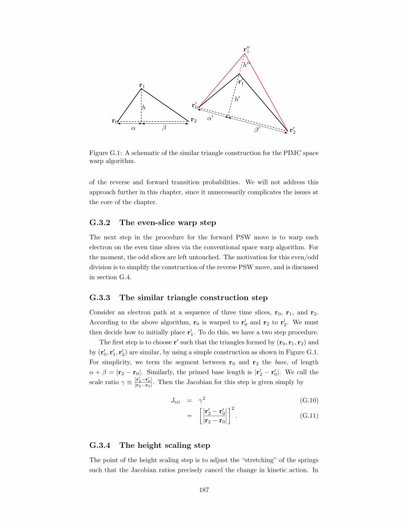
PSfrag replacements

r0

r1

r2

r′0

r′1

r′2

r′′1

hh′

h′′

α β

α′

β′

Figure G.1: A schematic of the similar triangle construction for the PIMC spacewarp algorithm.

of the reverse and forward transition probabilities. We will not address this

approach further in this chapter, since it unnecessarily complicates the issues at

the core of the chapter.

G.3.2 The even-slice warp step

The next step in the procedure for the forward PSW move is to warp each

electron on the even time slices via the conventional space warp algorithm. For

the moment, the odd slices are left untouched. The motivation for this even/odd

division is to simplify the construction of the reverse PSW move, and is discussed

in section G.4.

G.3.3 The similar triangle construction step

Consider an electron path at a sequence of three time slices, r0, r1, and r2.

According to the above algorithm, r0 is warped to r′0 and r2 to r′2. We must

then decide how to initially place r′1. To do this, we have a two step procedure.

The first step is to choose r′ such that the triangles formed by (r0, r1, r2) and

by (r′0, r′1, r

′2) are similar, by using a simple construction as shown in Figure G.1.

For simplicity, we term the segment between r0 and r2 the base, of length

α + β = |r2 − r0|. Similarly, the primed base length is |r′2 − r′0|. We call the

scale ratio γ ≡ |r′2−r′0||r2−r0| . Then the Jacobian for this step is given simply by

Jtri = γ2 (G.10)

=

[ |r′2 − r′0||r2 − r0|

]2

. (G.11)

G.3.4 The height scaling step

The point of the height scaling step is to adjust the “stretching” of the springs

such that the Jacobian ratios precisely cancel the change in kinetic action. In

187

this step, the heights, h′, of each triangle is scaled by a factor s, which may

be slightly greater or less than one, depending on whether the proposed ion

move and resulting space warp expands or contracts space on average. Here, we

construct the appropriate scale equation to determine s.

Let us first consider the transition probablilities for the forward and reverse

move. Let us assume, as is presently the case, the probabilities for selecting the

forward and reverse ion moves are equal, and hence their ratio is unity. Next, we

must consider the transition probilities for the space warp step. In section G.1.1,

we wrote down the Jacobian matrix, J , for the forward warp tranformation. We

may then writeTrev. warp

Tforw. warp= det(J). (G.12)

Next, we consider the similar triangle step. In this case again, the Jacobian for

the reverse move is the inverse of the Jacobian for the forward move. Hence,

Trev. tri

Tforw. tri=

[ |r′2 − r′0||r2 − r0|

]2

. (G.13)

Finally, we consider the height scaling step itself. Since it is a one-dimensional

scaling, its Jacobian is just s. Then

Trev. scale

Tforw. scale= s. (G.14)

The transition probability ratio for full PSW move will the the product of the

above ratios over all time slices and electrons. It is thus convenient to work

with logarithms. Define

Jwarp ≡∑

n,i

ln

[Trev. warp

Tforw. warp(ri

n)

]

, (G.15)

where the index n is over the odd slices and i is over electrons. Similarly, define

Jtri and Jscale with the time slice sum over the odd slices rather than the even.

Now, let us determine the change in the kinetic action as a function of the

scale factor, s.

Kold =1

4λτ(α2 + β2 + 2h2) (G.16)

Knew =1

4λτ(α′2 + β′2 + 2h′′2) (G.17)

=1

4λτγ2(α2 + β2 + 2s2h2) (G.18)

∆K(s) =γ2 − 1

4λτ(α2 + β2) +

1

4λτ2(γ2s2 − 1)h2 (G.19)

=1

4λτ

[(γ2 − 1)(α2 + β2)− 2h2 + 2γ2h2s2

]. (G.20)

188

We again sum over all even time slices and electrons,

∆K(s) ≡∑

n,i

∆K(s)n,i. (G.21)

We are now in the position to write down the equation for determining the

height scale factor, s.

Jwarp + Jtri + Jscale(s)−∆K(s) = 0. (G.22)

Using our definitions for Jscale and ∆K, we can rewrite this equation as

As2 +B ln(s) + C = 0, (G.23)

where

A = − 1

4λτ

∑

n,i∈odd

2γ2i h

2i (G.24)

B = NModd (G.25)

C = Jwarp + Jtri −∑

i∈even

(γ2i − 1)(α2

i + β2i )− 2h2

i

4λτ, (G.26)

where N is the number of electrons and Modd is the number of odd slices. We

can solve this transcendental equation iteratively with Newton’s method as

si+1 = si −As2i +B ln(si) + C

2Asi + Bsi

, (G.27)

starting with the initial guess, s0 = 1.

G.4 The inverse of the PIMC space warp

As mentioned above, we must be able to construct the reverse of our PIMC

space warp move in order to obey detailed balance. In the simplest approach,

we would simply apply each of our inverse steps in reverse order, i.e. we would

first invert the height scaling, then invert the similar triangle construction, invert

the warp, and finally invert the ion move.

Unfortunately, inverting the triangle height scaling cannot be done first, since

we do not know what scaling factor we would have chosen for the forward move.

However, the similar triangle construction and scaling operations commute, and

hence we may reorder. Next we note that space-warped even slices do not

depend on the odd slices. Hence, our first step in the reverse PIMC space warp

will be to invert the warps on the even slices, as described above. Next, we can

perform the similar triangle construction in the reverse direction. Once this is

done, we can determine what height scaling factor, s, would have satisfied the

scale equation. Finally, we invert the ion move. This algorithm is summarized

189

below.

1. First, perform the inverse warp tranformation on the electrons in the even

slices.

2. Perform the inverse of the similar triangle construction.

3. Solve the scale equation to determine the s the forward move would have

taken.

4. Invert the ion move.

In practice, this move is identical to the forward move, with the exception that

it uses the inverse warp rather than the forward warp.

It may have seemed to the reader that the triangle construction was a bit

awkward or unnecessarily complicated. After all, we could have simply warped

the odd slices as well as the even. If we had done so, however, determining

the reverse move would have been much more difficult. The commutability of

operations with the triangle construction makes constructing the inverse easy.

G.5 The failure of the method

In the above discussion, we failed to consider a subtle, but signficant contribu-

tion to the space warp Jacobian. In particular, we have neglected the fact that

the choice of the scaling factor, s, depends on the positions of the electrons at

every slice. Thus, the Jacobian for the scaling step is not simply s as we had

originally surmised. Thus, the equation we solved to determine s, (G.22), will

involve the derivatives of s with respect to the particle positions. We believe

that this differential equation will have no nontrivial solution. This reflects what

appears to be a general problem of any algorithm which attempts to increase the

acceptance ratio of a Monte Carlo move by an a posteriori correction. That is,

if our transition probability ratio is causing poor acceptance, this is because our

move does not sample the target distribution well. Trying to correct this after

the fact by nudging our state variables in such a way that the transition ratio

is cancelled by the change in energy/action will always run into this problem of

internal consistency.

Our space warp is essentially fixed by the proposed change to the ion posi-

tions. If the proposal is entirely independent of the electron positions, we will

always run into the problem we just described. If one is to construct an effi-

cient space warp method for PIMC, it must then involve proposing a change to

the ions that depends on the present positions of the electrons. Unfortunately,

doing so may become complicated very quickly.

190

References

[1] Claudia Filippi and C.J. Umrigar. Correlated sampling in quantum Monte

Carlo: A route to forces. Phys. Rev. B., 61(24):R16291, 15 June 2000.

191

Appendix H

PH pair density matricesthrough matrix squaring in3D

H.1 The pseudohamiltonian

We recall from Chapter 3 that the pseudohamiltonian operator can be written

in the radial form,

hps = −1

2

[dA

dr+

2A

r

]d

dr− 1

2Ad2

dr2+

B

2r2L2 + V (r). (H.1)

Beginning with the Schrodinger equation,

hpsψ(r) = Eψ(r), (H.2)

we would like cast the form of hps, through appropriate transformations, into

a more canonical form. Let us begin by considering the radial derivatives. We

draw from our experience in studying the radial equation in Chapter 4. We

showed that we can use the transformations,

x(r) ≡∫ r

0

dr′ A− 12 (r′) (H.3)

ψ(r) ≡ u(r)

rYlm(Ω) (H.4)

q(x) = A(r)14u(r) (H.5)

Veff(r) =1

2r

dA

dr− 1

32A

(dA

dr

)2

+1

8

d2

dA2+ V (r) (H.6)

to rewrite our eigenvalue problem as

− λ d2q

dx2+

[

λB(r)

r2L2 + Veff(r)

]

q(x) = Eq(x). (H.7)

Now, define

B(x) ≡ B(r)x2

r2. (H.8)

Then [

λ

(

− d2

dx2+B(x)

x2L2

)

+ Veff(r(x))

]

q(x) = Eq(x). (H.9)

192

Define

Ψ(x) ≡ q(x)

xYlm(Ω). (H.10)

Translating to vector notation, we obtain

[

λ

(

−∇2x +B(x)− 1

x2L2

)

+ Veff(r(x))

]

︸ ︷︷ ︸

Hps

Ψ(x) = EΨ(x). (H.11)

H.2 The density matrix

We ultimately seek to find the density matrix, defined as

ρ(r, r′;β) ≡⟨

r|e−βhps |r′⟩

. (H.12)

Rewriting as a sum in the energy eigenbasis, we have

ρ(r, r′;β) =∑

N

e−βENψ∗(r)ψ(r′) (H.13)

=∑

nlm

e−βEnlmunl(r)

rY ∗

lm(Ω)unl(r

′)

r′Ylm(Ω′) (H.14)

= [A(r)A(r′)]−14xx′

rr′

∑

nlm

e−βEnlqnl(x)

xY ∗

lm(Ω)qnl(x)

xYlm(Ω′)(H.15)

= [A(r)A(r′)]−14xx′

rr′

⟨

x

∣∣∣e−βHps

∣∣∣x

′⟩

(H.16)

= [A(r)A(r′)]−14xx′

rr′ρ(x,x′;β). (H.17)

As we shall see, it will be easier for us to work with the transformed Hamiltonian

Hps than with hps.

For clarity, we now define the action, S, as

S(x,x′;β) ≡ − ln [ρ(x,x′;β)] . (H.18)

For numerical reasons, we will divide the action into a kinetic part, T , and a

potential part, U , i.e. S = T + U . We furthermore divide T into a numerically

tabulated part, K and an analytic approximation, A, so that S = K + A + U .

U and K will be tabulated on a 3D grid and interpolated with tricubic splines.

A is giving by the following analytic form,

exp [−A(x,x′;β)] =

√

det(C)

π3exp [−〈x− x′|C|x− x′〉] . (H.19)

Here, C is a 3 × 3 matrix, which we presently define. Let U † be defined as a

193

3× 3 matrix whose rows are comprised of the unit vectors, r, θ, and φ, as

U † ≡

r

θ

φ

. (H.20)

Also, define Q as

Q ≡

(4λβ)−1 0 0

0 (4B(x)λβ)−1 0

0 0 (4B(x)λβ)−1

. (H.21)

The unit vectors can be computed by the following:

r =x

|x| (H.22)

φ =z × r|z × r| (H.23)

θ = φ× r. (H.24)

Then C is given by

C = UQU †. (H.25)

Note that this form for A(x,x′;β) is not perfectly symmetric in x and x′. If

we chose such a form, exp(−A) would a gaussian in neither x nor x′. The

form we chose was to be a perfect gaussian in x′. However, we must have that

T (x,x′;β) is symmetric. Thus neither the numerical A and the tabulated Kwill be symmetric, but their sum will be nonetheless. In particular, we may

write

A(x,x′;β) +K(x,x′;β) = A(x′,x;β) +K(x′,x;β). (H.26)

Then

K(x′,x;β) = K(x,x′;β) +A(x,x′;β)−A(x′,x;β). (H.27)

This implies that we need only store only half of K, such as for |x| > |x′|. Of

course, since U is symmetric, it need only be stored in this range as well. Finally,

we note that the quantity used in the actual squaring process, A(x,x′′;β) +

A(x′,x′′;β), is symmetric in x and x′.

H.3 Matrix squaring

We start by writing the density matrix in transformed coordinates as

ρ(x,x′;β) ≡⟨

x|e−βHps |x′⟩

(H.28)

=

⟨

x|e−βHps

2 e−βHps

2 |x′⟩

. (H.29)

194

Inserting a complete set of states,

ρ(x,x′;β) =

∫

d3x′′⟨

x|e−βHps

2 |x′′⟩⟨

x′′|e−βHps

2 |x′⟩

(H.30)

=

∫

d3x′′ρ(x,x′′;β/2)ρ(x′′,x′;β/2). (H.31)

Thus, by means of an integration (squaring the density matrix), we may reduce

the temperature of a density matrix by a factor of two. If an accurate approxi-

mation for the density matrix can be made at high temperature, we may start

at very small β and repeatedly “square” the temperature down to our desired

temperature.

H.3.1 Representation

The density matrix, ρ, is a function of six spatial dimensions, x and x′. Because

of the spherical symmetry of the Hamiltonian, however, this may be reduced to

three dimensions. The most intuitive coordinates are |x|, |x′|, and θ, the angle

between x and x′. However, we will find it more efficient and convenient to use

the set of coordinates defined by

q ≡ |x|+ |x′|2

(H.32)

z ≡ |x| − |x′| (H.33)

s ≡ |x− x′|. (H.34)

For the sake of the accuracy of numerical interpolation, it is generally desirable

to store the action, S, than the density matrix, ρ. Furthermore, it is important

to store the kinetic part of the action, K, separately from the potential part, U .

This is critical at high temperature since K ∝ β−1, while U ∝ β, and K would

completely wash out the meaningful information in U in that regime.

In order to separate K and U , we must have two separate, but parallel

squaring processes. In the first one, we will square down only K, neglecting the

potential terms. In the second, we will include the potential terms. Since we

have the result from K alone, we can isolate the effect of the potential, resulting

in undiminished information about its effect.

H.3.2 Grid considerations: information expansion

At very high temperatures, all of the relevant information about the density

matrix is contained near the diagaonal, i.e. x ≈ x′. In particular, as we shall

show, it is only necessary to tabulate the density matrix for a certain number

of σ’s away from the diagonal, where σ ≡√

2λβ. In our reduced coordinates,

this means that we need only store some restricted range of z and s.

To see why this is the case, consider calculating the value of the action at a

set of coordinates (q, z, s). We then translate into (x,x′) coordinates. We then

195

calculate an x which will be somewhere near 12 (x + x′). The free-particle part

of the action will then constrain the relevant part of the integral to within some

number of σ′s from x. Thus, we will need to have the action tabulated at the

previous level up to a distance of 12 |x− x′|+Nσ, where is N is some constant

depending on the quadrature rule used.

Recall that σ ∝√β. Thus, we see that with each squaring, we must increase

the range of values from the diagonal that we store by a factor of√

2. Working

through some typical values, we need store U and K for z and s up to about

60σ, to retain very high accuracy.

Let us define zcut and scut as the maximum tabulated value of those variables.

Then, we define

zmax ≡ min(zcut, 2q) (H.35)

smax ≡ min(scut, 2q) (H.36)

y ≡ z

zmax(H.37)

t ≡ s− |z|smax − |z|

. (H.38)

so that we may tabulate U(q, y, t) on a regular box-shaped mesh.

H.3.3 Integration

The kinetic part

By definition, we have that

exp[−T (x,x′; 2β)] =

∫

d3x′′ exp[−T (x,x′′;β)] exp[−T (x′,x′′;β)]. (H.39)

With T = K +A, we may then define

F (x,x′′,x′) ≡ exp [−K(x,x′′;β)−K(x′,x′′;β)] , (H.40)

and

G(x,x′′,x′) ≡ exp [−A(x,x′′;β)−A(x′,x′′;β) +A(x,x′; 2β)] . (H.41)

Thus we have

exp[−K] =

∫

d3x′′ F (x,x′′,x′)G(x,x′′,x′). (H.42)

Let us consider more carefully the form of G. Let C and C ′ be the generalized

gaussian width matrices corresponding to x and x′, respectively at inverse tem-

perature β. Then at inverse temperature 2β, the matrix corresponding to x is

196

C/2, since the width matrix is proporitional to β−1. Then, we may write that

G(x,x′′,x′) =

√

8 det(C ′)

π3exp [−〈x|C|x′′〉 − 〈x′|C ′|x′′〉+ 〈x|C/2|x′〉] (H.43)

Now, from section F.4, we recognize that if we define,

|x〉 ≡ (C + C ′)−1 [C|x〉+ C ′|x′〉] (H.44)

C ≡ C(C + C ′)−1C ′ − C

2(H.45)

C ≡ C + C ′, (H.46)

then we may rewrite,

G(x,x′′,x′) =

√

8 det(C ′)

π3exp

[−〈x′′ − x|C|x′′ − x〉

]exp

[

−〈x− x′|C|x− x′〉]

.

(H.47)

Hermite integration

Since G has a gaussian form in the variable of integration, Hermite integration

is particularly well-suited to this task. We now address specifically how this

may be done. We begin with the canonical form for a Hermite integration,

∫ ∞

−∞dx f(x)e−x2 ≈

∑

i

wif(xi)e−x2

i , (H.48)

where the sum is over an N -point rule with abcissas, xi, and weights wi. For

3D, we may then construct a product rule of the form,

∫

d3r f(r)e−r2

=∑

i,j,k

wiwjwkf(xi, xj , xk)f(r)e−r2

. (H.49)

Define, for convenience, WI ≡ wiwjwk and rI ≡ (xi, yj , zk) Consider an integral

now of the form, ∫

d3x′′ f(x′′)e−〈x′′−x|C|x′′−x〉 (H.50)

Now let us define |r〉 ≡ L†|x′′ − x〉, where LL† = C, calculated by Cholesky

decomposition. Then 〈r|r〉 = 〈x′′ − x|C|x′′ − x〉 and d3r = det(L)d3x′′. Then

we may write

∫

d3x′′ f(x′′)e−〈x′′−x|C|x′′−x〉 =1

det(L)

∫

d3r f([L†]−1 |r〉+ |x〉

)

e−〈r|r〉

=1

det(L)

∑

I

WIf([L†]−1 |rI〉+ |x〉

)

e−r2I

(H.51)

197

So, finally,

exp[−K(x,x′; 2β)] =√

8

π3

det(C ′)

det(C)exp

[

−〈x− x′|C|x− x′〉]∑

I

WI exp [−K(x,x′′I ;β)−K(x′,x′′

I ;β)] ,

(H.52)

where x′′I ≡

[L†]−1 |r〉+ |x〉. For sake of computational speed, we define WI ≡

WIe−r2

I .

As a sanity check, consider x = x′. Then C = 2C ′ and the arguments of

both exponentials on the RHS is zero.∑

IWI = π32 . Thus, the RHS = 1 and

K(x,x′; 2β) = 0, as expected.

H.4 The high-temperature approximation

Let us define Hps ≡ T + V , where

T = λ

(

−∇2x +B(x)− 1

x2L2

)

(H.53)

V = Veff(r(x)). (H.54)

We wish to have an approximation for 〈x| exp(−βHps)|x′〉 at very small β.

Since ρ must be symmetric, we need a symmetric approximation. Let C be the

gaussian width matrix at x and C ′ that for x′. We then define

C ≡ 2C(C + C ′)−1C ′ (H.55)

We can then create a symmetric approximation as

ρ(x,x′;β) ≈

√

det(C)

π3exp

[

−〈x− x′|C|x− x′〉]

exp (−βVavg) (H.56)

where

Vavg ≡∫ 1

0

dξ Veff [r(|ξx + (1− ξ)x′|)] . (H.57)

H.5 Problems with the method

Unfortuately, the high-temperature approximation given in the previous section

does not appear to be accurate enough. In particular, the variation of the

tangential mass with r makes it extremely difficult to properly normalize our

estimate for the kinetic part of the density matrix. If the variation of the inverse

mass is sufficiently small, it may still be possible to an accurate density matrix

with this method, but we have only found success when applying it to local

potentials. In this latter case, we can achieve fairly accurate results.

198

Appendix I

Cubic splines in one, two,and three dimensions

During our PIMC simulation, we need to evaluate the value and gradient of our

determinant wave function many millions of times. As a result, it is crucial we

have a fast method for such an evaluation. In this chapter, we will describe a

method to do this based on tricubic splines.

I.1 Cubic splines

Let us consider the problem in which we have a function y(x) specified at a

discrete set of points xi, such that y(xi) = yi. We wish to construct a piece-

wise cubic polynomial interpolating function, f(x), which satisfies the following

conditions:

• f(xi) = yi

• f ′(x−i ) = f ′(x+i )

• f ′′(x−i ) = f ′′(x+i ),

i.e. we require that the interpolating polynomials match in value and in their

first two derivatives at the connection points, xi.

I.1.1 Hermite interpolants

In our piecewise representation, we wish to store only the values, yi, and first

derivatives, y′i, of our function at each point xi, which we call knots. Given this

data, we wish to construct the piecewise cubic function to use between xi and

xi+1 which satisfies the above conditions. In particular, we wish to find the

unique cubic polynomial, P (x) satisfying

P (xi) = yi (I.1)

P (xi+1) = yi+1 (I.2)

P ′(xi) = y′i (I.3)

P ′(xi+1) = y′i+1. (I.4)

199

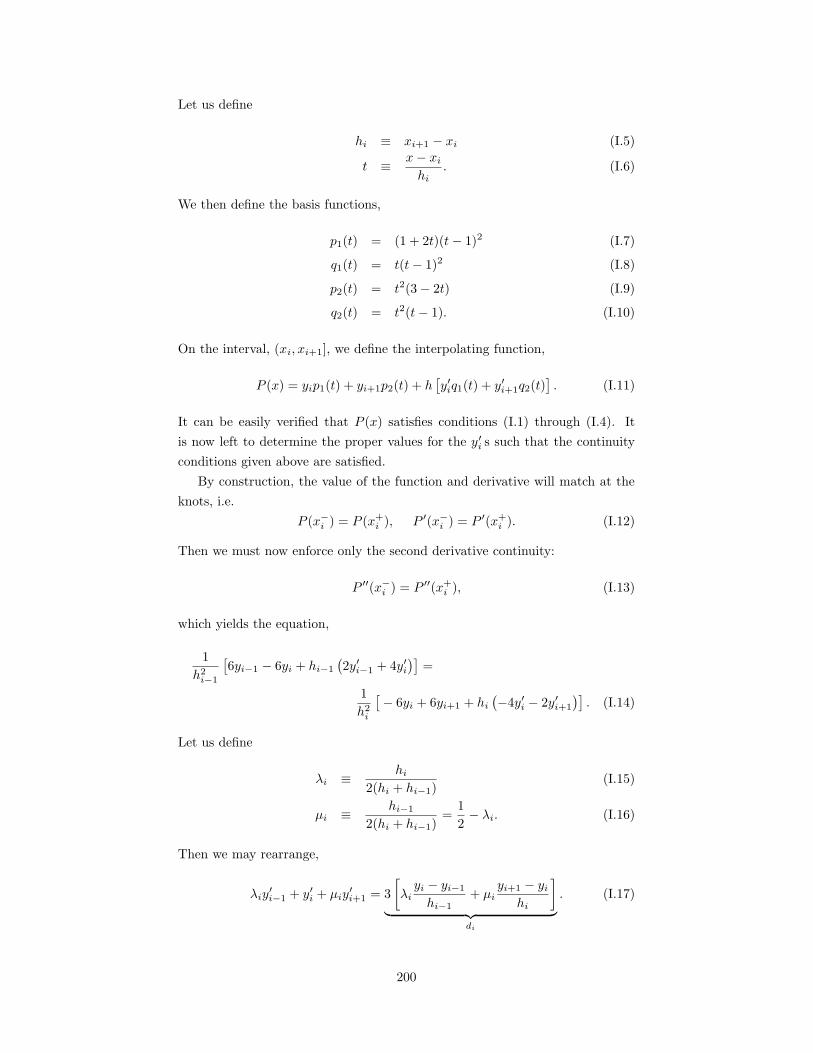
Let us define

hi ≡ xi+1 − xi (I.5)

t ≡ x− xi

hi. (I.6)

We then define the basis functions,

p1(t) = (1 + 2t)(t− 1)2 (I.7)

q1(t) = t(t− 1)2 (I.8)

p2(t) = t2(3− 2t) (I.9)

q2(t) = t2(t− 1). (I.10)

On the interval, (xi, xi+1], we define the interpolating function,

P (x) = yip1(t) + yi+1p2(t) + h[y′iq1(t) + y′i+1q2(t)

]. (I.11)

It can be easily verified that P (x) satisfies conditions (I.1) through (I.4). It

is now left to determine the proper values for the y′i s such that the continuity

conditions given above are satisfied.

By construction, the value of the function and derivative will match at the

knots, i.e.

P (x−i ) = P (x+i ), P ′(x−i ) = P ′(x+

i ). (I.12)

Then we must now enforce only the second derivative continuity:

P ′′(x−i ) = P ′′(x+i ), (I.13)

which yields the equation,

1

h2i−1

[6yi−1 − 6yi + hi−1

(2y′i−1 + 4y′i

)]=

1

h2i

[− 6yi + 6yi+1 + hi

(−4y′i − 2y′i+1

)]. (I.14)

Let us define

λi ≡ hi

2(hi + hi−1)(I.15)

µi ≡ hi−1

2(hi + hi−1)=

1

2− λi. (I.16)

Then we may rearrange,

λiy′i−1 + y′i + µiy

′i+1 = 3

[

λiyi − yi−1

hi−1+ µi

yi+1 − yi

hi

]

︸ ︷︷ ︸

di

. (I.17)

200

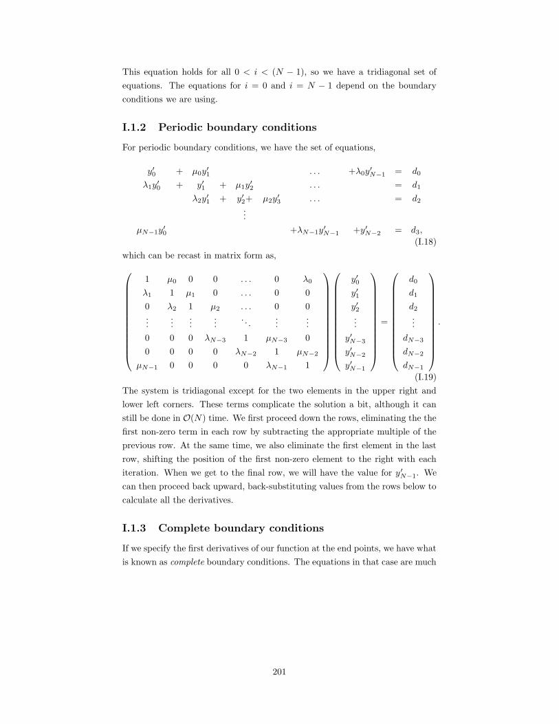
This equation holds for all 0 < i < (N − 1), so we have a tridiagonal set of

equations. The equations for i = 0 and i = N − 1 depend on the boundary

conditions we are using.

I.1.2 Periodic boundary conditions

For periodic boundary conditions, we have the set of equations,

y′0 + µ0y′1 . . . +λ0y

′N−1 = d0

λ1y′0 + y′1 + µ1y

′2 . . . = d1

λ2y′1 + y′2+ µ2y

′3 . . . = d2

...

µN−1y′0 +λN−1y

′N−1 +y′N−2 = d3,

(I.18)

which can be recast in matrix form as,

1 µ0 0 0 . . . 0 λ0

λ1 1 µ1 0 . . . 0 0

0 λ2 1 µ2 . . . 0 0...

......

.... . .

......

0 0 0 λN−3 1 µN−3 0

0 0 0 0 λN−2 1 µN−2

µN−1 0 0 0 0 λN−1 1

y′0y′1y′2...

y′N−3

y′N−2

y′N−1

=

d0

d1

d2

...

dN−3

dN−2

dN−1

.

(I.19)

The system is tridiagonal except for the two elements in the upper right and

lower left corners. These terms complicate the solution a bit, although it can

still be done in O(N) time. We first proceed down the rows, eliminating the the

first non-zero term in each row by subtracting the appropriate multiple of the

previous row. At the same time, we also eliminate the first element in the last

row, shifting the position of the first non-zero element to the right with each

iteration. When we get to the final row, we will have the value for y′N−1. We

can then proceed back upward, back-substituting values from the rows below to

calculate all the derivatives.

I.1.3 Complete boundary conditions

If we specify the first derivatives of our function at the end points, we have what

is known as complete boundary conditions. The equations in that case are much

201

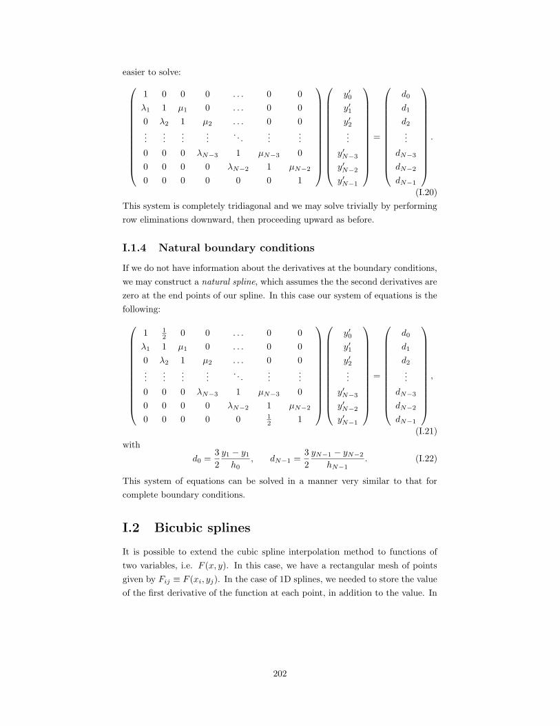
easier to solve:

1 0 0 0 . . . 0 0

λ1 1 µ1 0 . . . 0 0

0 λ2 1 µ2 . . . 0 0...

......

.... . .

......

0 0 0 λN−3 1 µN−3 0

0 0 0 0 λN−2 1 µN−2

0 0 0 0 0 0 1

y′0y′1y′2...

y′N−3

y′N−2

y′N−1

=

d0

d1

d2

...

dN−3

dN−2

dN−1

.

(I.20)

This system is completely tridiagonal and we may solve trivially by performing

row eliminations downward, then proceeding upward as before.

I.1.4 Natural boundary conditions

If we do not have information about the derivatives at the boundary conditions,

we may construct a natural spline, which assumes the the second derivatives are

zero at the end points of our spline. In this case our system of equations is the

following:

1 12 0 0 . . . 0 0

λ1 1 µ1 0 . . . 0 0

0 λ2 1 µ2 . . . 0 0...

......

.... . .

......

0 0 0 λN−3 1 µN−3 0

0 0 0 0 λN−2 1 µN−2

0 0 0 0 0 12 1

y′0y′1y′2...

y′N−3

y′N−2

y′N−1

=

d0

d1

d2

...

dN−3

dN−2

dN−1

,

(I.21)

with

d0 =3

2

y1 − y1h0

, dN−1 =3

2

yN−1 − yN−2

hN−1. (I.22)

This system of equations can be solved in a manner very similar to that for

complete boundary conditions.

I.2 Bicubic splines

It is possible to extend the cubic spline interpolation method to functions of

two variables, i.e. F (x, y). In this case, we have a rectangular mesh of points

given by Fij ≡ F (xi, yj). In the case of 1D splines, we needed to store the value

of the first derivative of the function at each point, in addition to the value. In

202

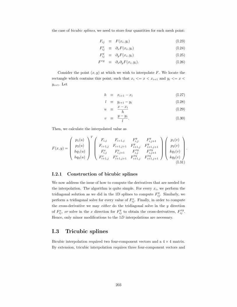
the case of bicubic splines, we need to store four quantities for each mesh point:

Fij ≡ F (xi, yi) (I.23)

F xij ≡ ∂xF (xi, yi) (I.24)

F yij ≡ ∂yF (xi, yi) (I.25)

F xy ≡ ∂x∂yF (xi, yi). (I.26)

Consider the point (x, y) at which we wish to interpolate F . We locate the

rectangle which contains this point, such that xi <= x < xi+1 and yi <= x <

yi+1. Let

h ≡ xi+1 − xi (I.27)

l ≡ yi+1 − yi (I.28)

u ≡ x− xi

h(I.29)

v ≡ y − yi

l. (I.30)

Then, we calculate the interpolated value as

F (x, y) =

p1(u)

p2(u)

hq1(u)

hq2(u)

T

Fi,j Fi+1,j F yi,j F y

i,j+1

Fi+1,j Fi+1,j+1 F yi+1,j F y

i+1,j+1

F xi,j F x

i,j+1 F xyi,j F xy

i,j+1

F xi+1,j F x

i+1,j+1 F xyi+1,j F xy

i+1,j+1

p1(v)

p2(v)

kq1(v)

kq2(v)

.

(I.31)

I.2.1 Construction of bicubic splines

We now address the issue of how to compute the derivatives that are needed for

the interpolation. The algorithm is quite simple. For every xi, we perform the

tridiagonal solution as we did in the 1D splines to compute F yij . Similarly, we

perform a tridiagonal solve for every value of F xij . Finally, in order to compute

the cross-derivative we may either do the tridiagonal solve in the y direction

of F xij , or solve in the x direction for F y

ij to obtain the cross-derivatives, F xyij .

Hence, only minor modifications to the 1D interpolations are necessary.

I.3 Tricubic splines

Bicubic interpolation required two four-component vectors and a 4× 4 matrix.

By extension, tricubic interpolation requires three four-component vectors and

203

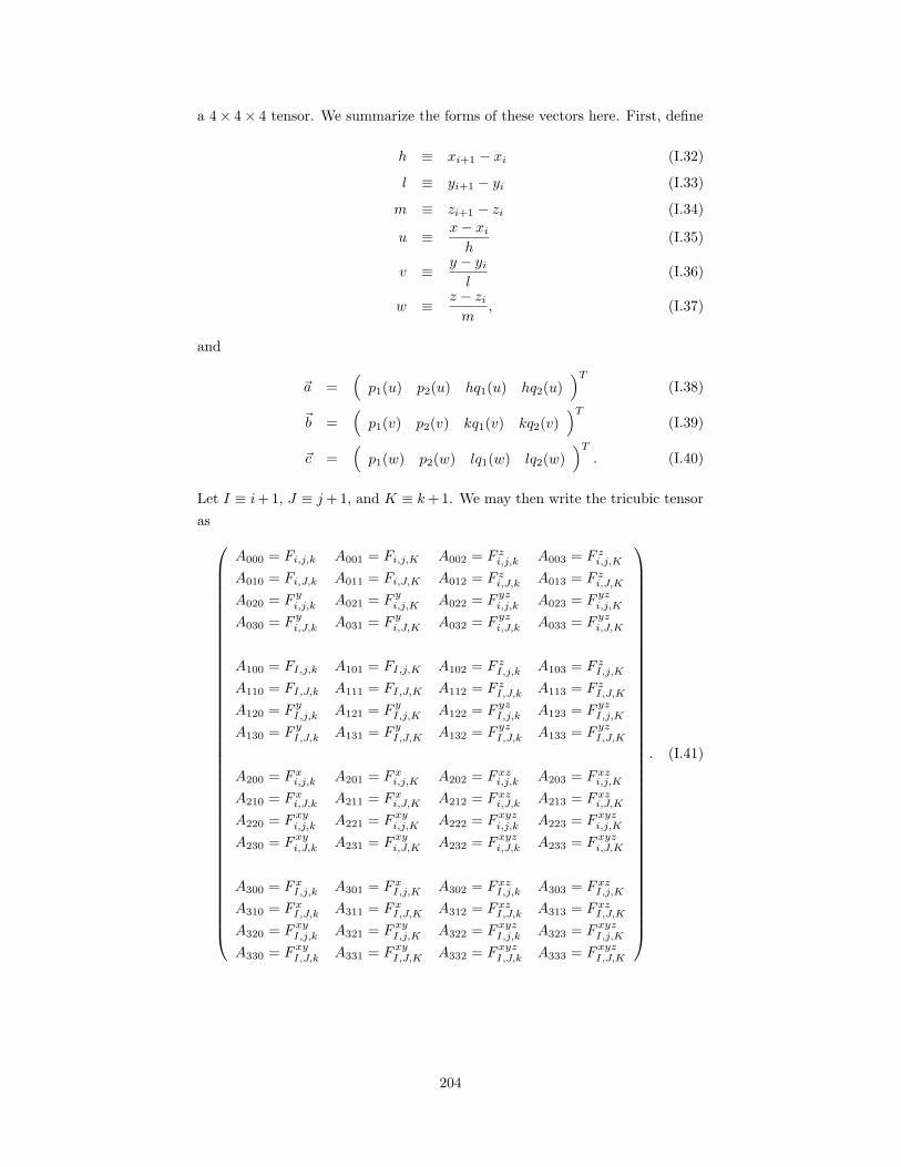
a 4× 4× 4 tensor. We summarize the forms of these vectors here. First, define

h ≡ xi+1 − xi (I.32)

l ≡ yi+1 − yi (I.33)

m ≡ zi+1 − zi (I.34)

u ≡ x− xi

h(I.35)

v ≡ y − yi

l(I.36)

w ≡ z − zi

m, (I.37)

and

~a =(

p1(u) p2(u) hq1(u) hq2(u))T

(I.38)

~b =(

p1(v) p2(v) kq1(v) kq2(v))T

(I.39)

~c =(

p1(w) p2(w) lq1(w) lq2(w))T

. (I.40)

Let I ≡ i+ 1, J ≡ j+ 1, and K ≡ k+ 1. We may then write the tricubic tensor

as

A000 = Fi,j,k A001 = Fi,j,K A002 = F zi,j,k A003 = F z

i,j,K

A010 = Fi,J,k A011 = Fi,J,K A012 = F zi,J,k A013 = F z

i,J,K

A020 = F yi,j,k A021 = F y

i,j,K A022 = F yzi,j,k A023 = F yz

i,j,K

A030 = F yi,J,k A031 = F y

i,J,K A032 = F yzi,J,k A033 = F yz

i,J,K

A100 = FI,j,k A101 = FI,j,K A102 = F zI,j,k A103 = F z

I,j,K

A110 = FI,J,k A111 = FI,J,K A112 = F zI,J,k A113 = F z

I,J,K

A120 = F yI,j,k A121 = F y

I,j,K A122 = F yzI,j,k A123 = F yz

I,j,K

A130 = F yI,J,k A131 = F y

I,J,K A132 = F yzI,J,k A133 = F yz

I,J,K

A200 = F xi,j,k A201 = F x

i,j,K A202 = F xzi,j,k A203 = F xz

i,j,K

A210 = F xi,J,k A211 = F x

i,J,K A212 = F xzi,J,k A213 = F xz

i,J,K

A220 = F xyi,j,k A221 = F xy

i,j,K A222 = F xyzi,j,k A223 = F xyz

i,j,K

A230 = F xyi,J,k A231 = F xy

i,J,K A232 = F xyzi,J,k A233 = F xyz

i,J,K

A300 = F xI,j,k A301 = F x

I,j,K A302 = F xzI,j,k A303 = F xz

I,j,K

A310 = F xI,J,k A311 = F x

I,J,K A312 = F xzI,J,k A313 = F xz

I,J,K

A320 = F xyI,j,k A321 = F xy

I,j,K A322 = F xyzI,j,k A323 = F xyz

I,j,K

A330 = F xyI,J,k A331 = F xy

I,J,K A332 = F xyzI,J,k A333 = F xyz

I,J,K

. (I.41)

204

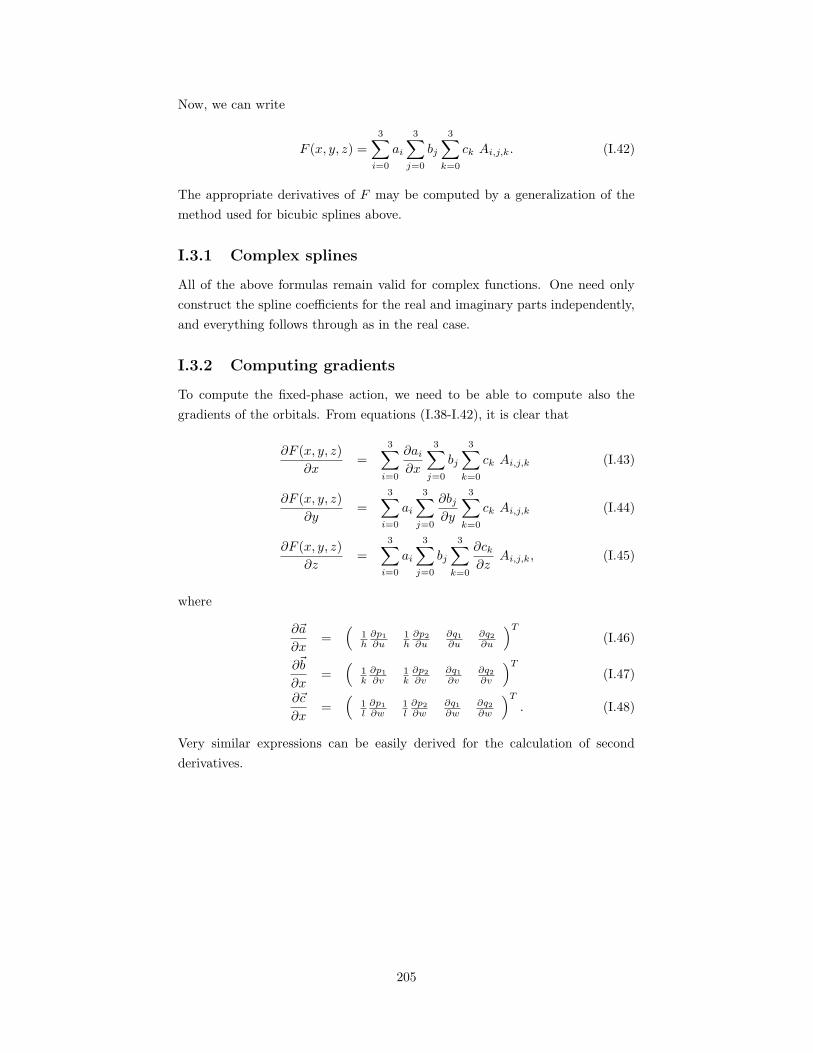
Now, we can write

F (x, y, z) =3∑

i=0

ai

3∑

j=0

bj

3∑

k=0

ck Ai,j,k. (I.42)

The appropriate derivatives of F may be computed by a generalization of the

method used for bicubic splines above.

I.3.1 Complex splines

All of the above formulas remain valid for complex functions. One need only

construct the spline coefficients for the real and imaginary parts independently,

and everything follows through as in the real case.

I.3.2 Computing gradients

To compute the fixed-phase action, we need to be able to compute also the

gradients of the orbitals. From equations (I.38-I.42), it is clear that

∂F (x, y, z)

∂x=

3∑

i=0

∂ai

∂x

3∑

j=0

bj

3∑

k=0

ck Ai,j,k (I.43)

∂F (x, y, z)

∂y=

3∑

i=0

ai

3∑

j=0

∂bj∂y

3∑

k=0

ck Ai,j,k (I.44)

∂F (x, y, z)

∂z=

3∑

i=0

ai

3∑

j=0

bj

3∑

k=0

∂ck∂z

Ai,j,k, (I.45)

where

∂~a

∂x=

(1h

∂p1

∂u1h

∂p2

∂u∂q1

∂u∂q2

∂u

)T

(I.46)

∂~b

∂x=

(1k

∂p1

∂v1k

∂p2

∂v∂q1

∂v∂q2

∂v

)T

(I.47)

∂~c

∂x=

(1l

∂p1

∂w1l

∂p2

∂w∂q1

∂w∂q2

∂w

)T

. (I.48)

Very similar expressions can be easily derived for the calculation of second

derivatives.

205

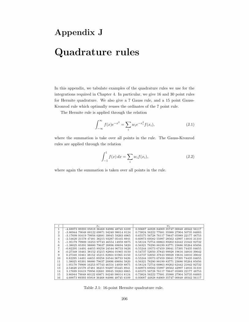
Appendix J

Quadrature rules

In this appendix, we tabulate examples of the quadrature rules we use for the

integrations required in Chapter 4. In particular, we give 16 and 30 point rules

for Hermite quadrature. We also give a 7 Gauss rule, and a 15 point Gauss-

Kronrod rule which optimally reuses the ordinates of the 7 point rule.

The Hermite rule is applied through the relation

∫ ∞

−∞f(x)e−x2

=∑

i

wie−x2

i f(xi), (J.1)

where the summation is take over all points in the rule. The Gauss-Kronrod

rules are applied through the relation

∫ 1

−1

f(x) dx =∑

i

wif(xi), (J.2)

where again the summation is taken over all points in the rule.

i xi wi

1 -4.68873 89393 05818 36468 84986 48745 6109 0.93687 44928 84069 35747 00048 49342 561172 -3.86944 79048 60122 69871 94240 98014 8124 0.73824 56222 77681 35988 27904 50735 840033 -3.17699 91619 79956 02681 39945 59263 6965 0.65575 56728 76117 70647 05989 22177 487534 -2.54620 21578 47481 36215 93287 05445 8941 0.60973 69582 55997 28562 42997 14816 313105 -1.95178 79909 16253 97743 46554 14959 8875 0.58124 72754 00863 89202 62442 21842 927326 -1.38025 85391 98880 79637 20896 69694 5820 0.56321 78290 88199 83771 23686 95264 850567 -0.82295 14491 44655 89258 24544 96733 9426 0.55244 19573 67459 39041 57395 74435 046558 -0.27348 10461 38152 45215 82804 01965 0150 0.54737 52050 37843 99928 19616 34810 390429 0.27348 10461 38152 45215 82804 01965 0150 0.54737 52050 37843 99928 19616 34810 3904210 0.82295 14491 44655 89258 24544 96733 9426 0.55244 19573 67459 39041 57395 74435 0465511 1.38025 85391 98880 79637 20896 69694 5820 0.56321 78290 88199 83771 23686 95264 8505612 1.95178 79909 16253 97743 46554 14959 8875 0.58124 72754 00863 89202 62442 21842 9273213 2.54620 21578 47481 36215 93287 05445 8941 0.60973 69582 55997 28562 42997 14816 3131014 3.17699 91619 79956 02681 39945 59263 6965 0.65575 56728 76117 70647 05989 22177 4875315 3.86944 79048 60122 69871 94240 98014 8124 0.73824 56222 77681 35988 27904 50735 8400316 4.68873 89393 05818 36468 84986 48745 6109 0.93687 44928 84069 35747 00048 49342 56117

Table J.1: 16-point Hermite quadrature rule.

206

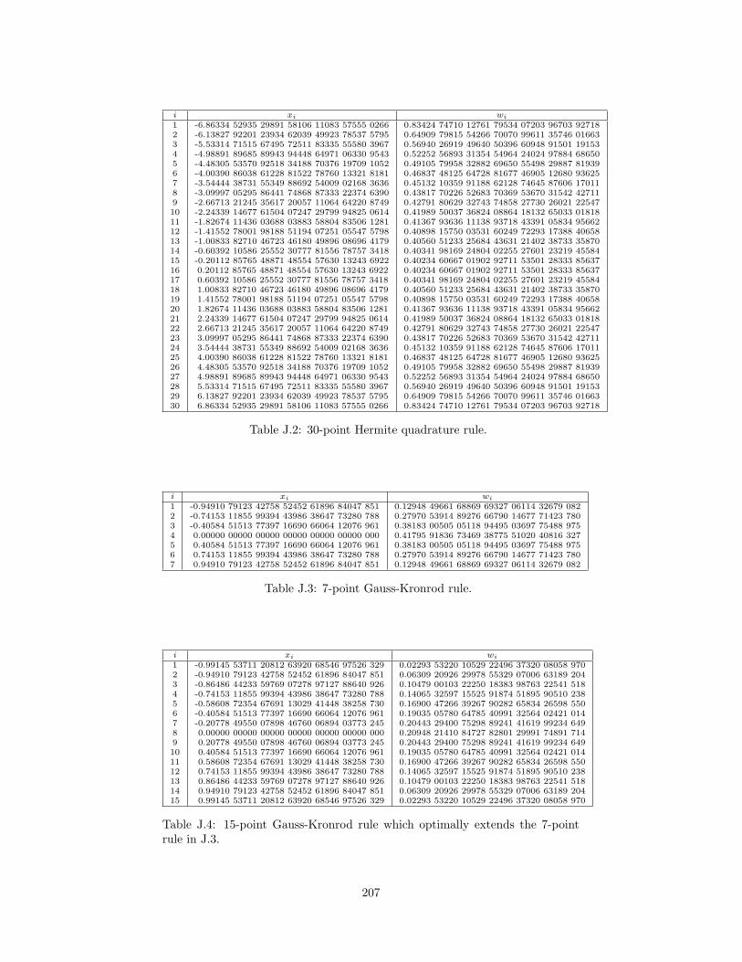
i xi wi

1 -6.86334 52935 29891 58106 11083 57555 0266 0.83424 74710 12761 79534 07203 96703 927182 -6.13827 92201 23934 62039 49923 78537 5795 0.64909 79815 54266 70070 99611 35746 016633 -5.53314 71515 67495 72511 83335 55580 3967 0.56940 26919 49640 50396 60948 91501 191534 -4.98891 89685 89943 94448 64971 06330 9543 0.52252 56893 31354 54964 24024 97884 686505 -4.48305 53570 92518 34188 70376 19709 1052 0.49105 79958 32882 69650 55498 29887 819396 -4.00390 86038 61228 81522 78760 13321 8181 0.46837 48125 64728 81677 46905 12680 936257 -3.54444 38731 55349 88692 54009 02168 3636 0.45132 10359 91188 62128 74645 87606 170118 -3.09997 05295 86441 74868 87333 22374 6390 0.43817 70226 52683 70369 53670 31542 427119 -2.66713 21245 35617 20057 11064 64220 8749 0.42791 80629 32743 74858 27730 26021 2254710 -2.24339 14677 61504 07247 29799 94825 0614 0.41989 50037 36824 08864 18132 65033 0181811 -1.82674 11436 03688 03883 58804 83506 1281 0.41367 93636 11138 93718 43391 05834 9566212 -1.41552 78001 98188 51194 07251 05547 5798 0.40898 15750 03531 60249 72293 17388 4065813 -1.00833 82710 46723 46180 49896 08696 4179 0.40560 51233 25684 43631 21402 38733 3587014 -0.60392 10586 25552 30777 81556 78757 3418 0.40341 98169 24804 02255 27601 23219 4558415 -0.20112 85765 48871 48554 57630 13243 6922 0.40234 60667 01902 92711 53501 28333 8563716 0.20112 85765 48871 48554 57630 13243 6922 0.40234 60667 01902 92711 53501 28333 8563717 0.60392 10586 25552 30777 81556 78757 3418 0.40341 98169 24804 02255 27601 23219 4558418 1.00833 82710 46723 46180 49896 08696 4179 0.40560 51233 25684 43631 21402 38733 3587019 1.41552 78001 98188 51194 07251 05547 5798 0.40898 15750 03531 60249 72293 17388 4065820 1.82674 11436 03688 03883 58804 83506 1281 0.41367 93636 11138 93718 43391 05834 9566221 2.24339 14677 61504 07247 29799 94825 0614 0.41989 50037 36824 08864 18132 65033 0181822 2.66713 21245 35617 20057 11064 64220 8749 0.42791 80629 32743 74858 27730 26021 2254723 3.09997 05295 86441 74868 87333 22374 6390 0.43817 70226 52683 70369 53670 31542 4271124 3.54444 38731 55349 88692 54009 02168 3636 0.45132 10359 91188 62128 74645 87606 1701125 4.00390 86038 61228 81522 78760 13321 8181 0.46837 48125 64728 81677 46905 12680 9362526 4.48305 53570 92518 34188 70376 19709 1052 0.49105 79958 32882 69650 55498 29887 8193927 4.98891 89685 89943 94448 64971 06330 9543 0.52252 56893 31354 54964 24024 97884 6865028 5.53314 71515 67495 72511 83335 55580 3967 0.56940 26919 49640 50396 60948 91501 1915329 6.13827 92201 23934 62039 49923 78537 5795 0.64909 79815 54266 70070 99611 35746 0166330 6.86334 52935 29891 58106 11083 57555 0266 0.83424 74710 12761 79534 07203 96703 92718

Table J.2: 30-point Hermite quadrature rule.

i xi wi

1 -0.94910 79123 42758 52452 61896 84047 851 0.12948 49661 68869 69327 06114 32679 0822 -0.74153 11855 99394 43986 38647 73280 788 0.27970 53914 89276 66790 14677 71423 7803 -0.40584 51513 77397 16690 66064 12076 961 0.38183 00505 05118 94495 03697 75488 9754 0.00000 00000 00000 00000 00000 00000 000 0.41795 91836 73469 38775 51020 40816 3275 0.40584 51513 77397 16690 66064 12076 961 0.38183 00505 05118 94495 03697 75488 9756 0.74153 11855 99394 43986 38647 73280 788 0.27970 53914 89276 66790 14677 71423 7807 0.94910 79123 42758 52452 61896 84047 851 0.12948 49661 68869 69327 06114 32679 082

Table J.3: 7-point Gauss-Kronrod rule.

i xi wi

1 -0.99145 53711 20812 63920 68546 97526 329 0.02293 53220 10529 22496 37320 08058 9702 -0.94910 79123 42758 52452 61896 84047 851 0.06309 20926 29978 55329 07006 63189 2043 -0.86486 44233 59769 07278 97127 88640 926 0.10479 00103 22250 18383 98763 22541 5184 -0.74153 11855 99394 43986 38647 73280 788 0.14065 32597 15525 91874 51895 90510 2385 -0.58608 72354 67691 13029 41448 38258 730 0.16900 47266 39267 90282 65834 26598 5506 -0.40584 51513 77397 16690 66064 12076 961 0.19035 05780 64785 40991 32564 02421 0147 -0.20778 49550 07898 46760 06894 03773 245 0.20443 29400 75298 89241 41619 99234 6498 0.00000 00000 00000 00000 00000 00000 000 0.20948 21410 84727 82801 29991 74891 7149 0.20778 49550 07898 46760 06894 03773 245 0.20443 29400 75298 89241 41619 99234 64910 0.40584 51513 77397 16690 66064 12076 961 0.19035 05780 64785 40991 32564 02421 01411 0.58608 72354 67691 13029 41448 38258 730 0.16900 47266 39267 90282 65834 26598 55012 0.74153 11855 99394 43986 38647 73280 788 0.14065 32597 15525 91874 51895 90510 23813 0.86486 44233 59769 07278 97127 88640 926 0.10479 00103 22250 18383 98763 22541 51814 0.94910 79123 42758 52452 61896 84047 851 0.06309 20926 29978 55329 07006 63189 20415 0.99145 53711 20812 63920 68546 97526 329 0.02293 53220 10529 22496 37320 08058 970

Table J.4: 15-point Gauss-Kronrod rule which optimally extends the 7-pointrule in J.3.

207

Author’s biography

Kenneth Paul Esler, Jr. was born in Ridgewood, New Jersey on October 13,

1976. He graduated from the Massachusetts Institute of Technology with a Sci-

ence Bachelors degree in physics with electrical engineering in 1999. In the Fall

of that year, he began graduate study in Urbana, Illinois under the advisement

of Prof. David Ceperley. He completed his doctorate in 2006 and has begun a

postdoctoral appointment at the Geophysical Laboratory of the Carnegie Insti-

tution of Washington, applying quantum Monte Carlo methods to the study of

minerals under pressure.

208