C-2 Eagle Project Geotechnical Study · PDF fileC-2 Eagle Project Geotechnical Study . Golder...

LJS\J:\scopes\04w018\10000\FVD reports\Final MPA\r-Mine Permit App appendix.doc

C-2

Eagle Project Geotechnical Study

Golder Associates Ltd. 662 Falconbridge Road Sudbury, Ontario, Canada P3A 4S4 Telephone: (705) 524-6861 Fax: (705) 524-1984

April 28, 2005 04-1193-020

OFFICES ACROSS NORTH AMERICA, SOUTH AMERICA, EUROPE, AFRICA, ASIA AND AUSTRALIA

REPORT ON

Submitted to:

Kennecott Exploration Company Rio Tinto Technical Services

5295 South 300 West, Suite 300 Murray, Utah

84107

Attention: Mr. Roger Sawyer

DISTRIBUTION: 2 Copies - Kennecott Exploration Company 2 Copies - Golder Associates Ltd., Sudbury, Ontario

EAGLE PROJECT GEOTECHNICAL STUDY

April 2005 - i - 04-1193-020

Golder Associates

EXECUTIVE SUMMARY

A geotechnical study has been completed for Kennecott Exploration’s Eagle Nickel deposit in the Upper Peninsula of Michigan, USA. Included in this geotechnical study is information regarding a data review of two geotechnical borehole databases for the Eagle Project. A geotechnical model was created using the information in the databases to infer rock mass quality, rock strength, and major discontinuities in the semi-massive/massive sulphide ore lens, the peridotite hangingwall and footwall and the sediments in the main decline and portal area. The geotechnical model was built using the GoCAD software. Representative horizontal and vertical contoured sections of rock mass quality and rock quality designation (RQD) were created in the GoCAD geotechnical model.

Based on these sections, a ground support assessment was completed on the various underground drift infrastructures. The results from the ground support assessment recommended a three-class support system which was based on rock mass quality and drift dimension. The three-class support system was defined as: systematic pattern bolting support for Q>4; systematic pattern bolting support and 4-10 cm of fibre reinforced shotcrete for Q<4 and Q>1; and systematic pattern bolting support, metal screen and 4-10 cm of plain shotcrete for Q<1. Details of the rock support assessment are presented in Section 4.0.

A stope stability assessment was completed using the Mathews Method based on the initial stope dimensions for transverse (15-60 m by 20 m by 30 m high) and longitudinal (5-15 m by 60 m by 30 m high) longhole mining as proposed in the AMEC Scoping Study. The results from the stope stability assessment indicated that the initial stope dimensions for transverse and longitudinal longhole mining are stable. A second stope stability assessment was completed by using 10% and 20% dilution along the walls of the transverse and longitudinal stopes and indicated that these diluted stopes were stable but may require support as well. This stope stability assessment was based on the inferred rock mass quality. The actual in situ rock mass conditions need to be incorporated in the final stope designs.

Several crown pillar assessments were completed using the empirical Scaled Span Method and a limit equilibrium assessment using the CPillar software. The last assessment considered stope geometries supplied by McIntosh within an AutoCAD sequencing model. The results of this assessment were that if the rock mass quality in the crown had a Rock Mass Rating (RMR) = 75, then no stopes could be mined in Level 1 in order to get a factor of safety of 1.9. Alternatively, if the rock mass quality in the crown had an RMR = 85, then three stopes (i.e., all of the high grade zones) could be mined in Level 1 with a factor of safety of 1.8. Details of the crown pillar assessments are presented in Sections 6.0 through 6.4. A discussion on additional crown pillar information requirements and assessment recommendations as the project proceeds underground is presented in Section 6.5.

April 2005 - ii - 04-1193-020

Golder Associates

An initial backfill strength assessment was completed for the primary/secondary stope panels proposed by McIntosh Engineering. This assessment identified the minimum strength required for the primary panels to be self-supporting when they are exposed on the east and west walls. Two methods were used to determine the minimum strengths: 2D vertical slope method and the Mitchell method. Using a factor of safety of 2, a strength requirement of 1.5 MPa (218 psi) was considered the minimum strength for the primary stopes panels (maximum stope dimensions 70 m north-south, 20 m east-west and 34.5 m high).

A review was completed for the proposed mining extraction sequence provided by McIntosh Engineering. A 3-dimensional numerical model was created using the Map3D software based on the proposed stope panel dimensions, extraction sequence and rock mass properties of the ore, waste and backfill types and an estimated stress regime. Two stress parameters were reviewed in the numerical model results: the minor principal stress and the difference between major and minor principal stress (deviatoric stress). The minor principal stress and deviatoric stress were considered to indicate potential issues due to relaxation and high stress, respectively. The Map3D results indicated that major stability problems due to induced stress conditions are not expected with the proposed mining sequence. Details of the modelling are presented in Section 8.0.

April 2005 - iii - 04-1193-020

Golder Associates

TABLE OF CONTENTS

SECTION PAGE

1.0 INTRODUCTION......................................................................................... 1 1.1 Objective................................................................................................1

2.0 DATA REVIEW ........................................................................................... 2 2.1 Borehole Data Review............................................................................2

3.0 GEOTECHNICAL MODEL.......................................................................... 4 3.1 Eagle Deposit General Lithology ............................................................4 3.2 GoCAD Model ........................................................................................4 3.3 Rock Strength ........................................................................................5 3.4 RQD.......................................................................................................7 3.5 Rock Mass Classification Systems.........................................................7

3.5.1 RMR Parameter of A1 ................................................................8 3.5.2 RMR Parameter A2 ....................................................................8 3.5.3 RMR Parameter A3 ....................................................................9 3.5.4 RMR Parameter A4 ....................................................................9 3.5.5 RMR Parameter A5 ..................................................................10

3.6 RMR Summary.....................................................................................10 3.7 Major Discontinuity Sets.......................................................................11 3.8 Discrete Features.................................................................................13

4.0 ROCK SUPPORT ASSESSMENT ........................................................... 14 4.1 Empirical Design Chart.........................................................................14 4.2 Mining Methods....................................................................................15 4.3 Support Classification ..........................................................................15 4.4 Bolt Length and Spacing ......................................................................17 4.5 Ground Support Pressure ....................................................................17 4.6 Pattern Support ....................................................................................18

4.6.1 Ground Support for Main Ramp................................................18 4.7 Kinematic Unwedge Analysis ...............................................................18

5.0 STOPE SIZING......................................................................................... 21 5.1 Matthews Stability Graph Method.........................................................21 5.2 Longitudinal Longhole Mining...............................................................22 5.3 Transverse Longhole Mining ................................................................22 5.4 Rock Stress Factor (A) .........................................................................23 5.5 Joint Orientation (B) .............................................................................24 5.6 Gravity Adjustment Factor (C) ..............................................................25 5.7 Stability Number (N’) ............................................................................26 5.8 Stope Dilution.......................................................................................27 5.9 Stope Sizing Discussion.......................................................................27

April 2005 - iv - 04-1193-020

Golder Associates

TABLE OF CONTENTS (CONTINUED)

6.0 CROWN PILLAR....................................................................................... 29 6.1 Crown Pillar Stability Assessment ........................................................29 6.2 Scaled Span Cs ....................................................................................29

6.2.1 Eagle Crown Pillar Scaled Span Assessment...........................30 6.3 CPillar Analysis ....................................................................................32

6.3.1 Eagle CPillar Analysis...............................................................32 6.4 Additional Crown Pillar Assessment .....................................................34 6.5 Crown Pillar Discussion and Recommendations ..................................34

7.0 BACKFILL DESIGN .................................................................................. 36 8.0 MINING SEQUENCE................................................................................ 38

8.1 Model Geometry and Mining Sequence ...............................................38 8.2 Modelling Material Parameters and Stress Regime..............................39 8.3 Modelling Results.................................................................................40

8.3.1 Minor Principal Stress...............................................................40 8.3.2 Deviatoric Stress Results..........................................................41

8.4 Mining Sequence Discussion ...............................................................42 9.0 HYDROGEOLOGY ................................................................................... 43 10.0 CLOSURE................................................................................................. 44

April 2005 - v - 04-1193-020

Golder Associates


LIST OF TABLES Table 1 Boreholes Used in GoCAD Model Table 2 ISRM Rock Strength Chart Table 3 Point Load Testing Data and UCS for Eagle Project Database Table 4 A1 Chart for RMR Table 5 RQD Rating for RMR Table 6 Discontinuity Spacing Rating for RMR Table 7 Discontinuity Condition for RMR Table 8 Eagle Project Rock Mass Classification Table 9 Discontinuity Sets for Semi-massive and Massive Sulphides Table 10 Discontinuity Sets for Peridotite and Feldspathic Peridotite Table 11 Discontinuity Sets for Siltstone and Sandstone Table 12 Major and Minor Discontinuity Sets Table 13 ESR Values for Excavation Categories after Barton et Al. (1974) Table 14 Drift Dimensions by Mining Method Table 15 Eagle Project Rock Mass Classification Table 16 HR for Longitudinal Longhole Mining Table 17 HR for Transverse Longhole Mining Table 18 Stability Number A Value Table 19 Stability Number B Value Table 20 Stability Number N’ vs. Qequiv

Table 21 Eagle Crown Pillar Assessment - Scaled Span (RMR = 75) Table 22 Eagle Crown Pillar Assessment - Scaled Span (RMR = 85) Table 23 Eagle Crown Pillar CPillar Analysis (RMR = 75) Table 24 Eagle Crown Pillar CPillar Analysis (RMR = 85) Table 25 Eagle Crown Pillar Assessment – Scaled Span Optimized Geometry Table 26 Minimum Strength of Backfill Design for Primary Stopes Table 27 Map3D Model Material Properties Table 28 Map3D Model Stress Regime Properties

April 2005 - vi - 04-1193-020

Golder Associates


LIST OF FIGURES Figure 1 Eagle Deposit Site Plan Figure 2 Eagle Deposit: Isometeric View of Geotechnical Drillhole Coverage Figure 3 Plan: RQD and RMR Contouring for 405 Elev. Figure 4 Plan: RQD and RMR Contouring for 355 Elev. Figure 5 Plan: RQD and RMR Contouring for 280 Elev. Figure 6 Plan: RQD and RMR Contouring for 220 Elev. Figure 7 Plan: RQD and RMR Contouring for 160 Elev. Figure 8 Plan: RQD and RMR Contouring for 100 Elev. Figure 9 Traverse Section: RQD and RMR Contouring for 431420E Facing East Figure 10 Traverse Section: RQD and RMR Contouring for 431457E Facing East Figure 11 Traverse Section: RQD and RMR Contouring for 431500E Facing East Figure 12 Traverse Section: RQD and RMR Contouring for 431545E Facing East Figure 13 Traverse Section: RQD and RMR Contouring for 431585E Facing East Figure 14 Longitudinal Section: RQD and RMR Contouring for 5177500N Facing North Figure 15 Longitudinal Section: RQD and RMR Contouring for 5177560N Facing North Figure 16 Major Discontinuity Sets (All Features) – Semi-Massive Sulphide and Massive

Sulphide Figure 17 Major Discontinuity Sets (All Features) – Peridotite and Feldspar Peridotite Figure 18 Major Discontinuity Sets (All Features) – Sandstone and Siltstone Figure 19 Rock Support Design Chart for Spans 5 m to 8 m Figure 20 Rock Support Design Chart for Intersection Spans 6.2 m to 8.8 m Figure 21 Unwedge Assessment 5 m High by 5 m Wide Figure 22 Unwedge Assessment 5 m High by 6.2 m Wide (Intersections) Figure 23 Unwedge Assessment 4.7 m High by 8.0 and 8.8 m Wide (Intersection) Figure 24 Transverse and Longitudinal Longhole Stope Face Stability Plot Figure 25 Transverse and Longitudinal Longhole End Walls Stability Plot Figure 26 Transverse and Longitudinal Longhole Stope Back Stability Plot Figure 27 Transverse and Longitudinal Stoping Dilution Figure 28 Cs Versus QEquiv for the Scaled Span Assessments Eagle Crown Pillar Figure 29 CPillar Output for the Eagle Crown Pillar Assessments Figure 30 Eagle Deposit – Map3D Model – Stope Labelling and Sequencing, View –

South Figure 31 Eagle Project – Map3D Model – Isometric View Figure 32 Eagle Project – Map3D – Sigma 3 Results, Grid 1 – Steps 11, 13, 16, 20, 23,

27, View – South Figure 33 Eagle Project – Map3D – Sigma 3 Results – Secondary Panels - Grid 2 –

Steps 11, 13, 14, 17, 19, 27 – View – West Figure 34 Eagle Project – Map3D – Sigma 3 Results – Grid 1, 2, 3 and 4 – North &

South Wall Figure 35 Eagle Project – Map3D – Deviatoric Stress Results – Grid 1, 2, 3 and 4 –

North and South Wall

April 2005 - vii - 04-1193-020

Golder Associates


LIST OF APPENDICES Appendix A Lithological Sections A1 to A12 Provided by KEX Appendix B Rock Mass Classification Systems

April 2005 - 1 - 04-1193-020

Golder Associates

1.0 INTRODUCTION

The Eagle Project is a nickel deposit owned by Kennecott Exploration Company (KEX) located in the Upper Peninsula of Michigan, USA. Golder Associates Ltd. (Golder) has been retained by KEX to provide a geotechnical design study as part of an overall prefeasibility study for the Eagle Project. Illustrated on Figure 1 is a plan drawing indicating the location of the portal, the main ramp and main mining zones.

1.1 Objective

The objective of this study is to provide geotechnical design input to assist in the preparation of a prefeasibility study, with an accuracy of ±25%, to evaluate the alternatives for developing the Eagle Project.

April 2005 - 2 - 04-1193-020

Golder Associates

2.0 DATA REVIEW

The geotechnical logging database (dated January 3, 2005) from the ongoing drilling program at the Eagle deposit has been reviewed. Currently, the data is organised into two Microsoft Access databases based on when they were drilled; pre-2004 and 2004. The databases were created using custom entry forms and consist of tables including those describing cemented joints, open joints, basic geotechnical measurements, major structures and point load tests. Some entries were found to be deficient in information. A list of deficient data has been formulated and communicated to KEX personnel on site.

Geotechnical logging is completed in Marquette by a team of geologists. Drill core is processed by the geologists after it has been boxed on site by the drillers. Logging procedures have been formulated and revised from 2001 to present. This has resulted in a marked improvement in the quality and completeness of the data over this period. Currently, the geologists are logging according to the procedures outlined in “EAGLE PROJECT: DATA COLLECTION AND ANALYSIS PROCEDURES, 2001 – 2003” (Coombes, 2004) which follows standard Rio Tinto and industry recognised geotechnical core logging practices.

Basic geotechnical measurements are given over a 3 m interval (based on run length) and consist of rock type, total core recovery (TCR), solid core recovery (SCR), intact rock strength (R-value) and Rock Quality Designation (RQD). Cemented joint data is based on sets. Data for each set includes the depth interval (from surface along borehole), the number of features, the alpha angle, the beta angle (when available), the type of joint infill and the relative strength of the joint(s). Open joint data is based on sets and the data collected is the same as that for cemented joints with the exception that joint wall condition is logged rather than relative joint strength. Three separate parameters are used to log the joint wall condition: joint roughness, joint alteration and joint infill. Axial and diametric point load test data exists for the majority of the basic rock types. A procedure is currently in place to photograph and catalogue core photos (wet and dry).

2.1 Borehole Data Review

The Microsoft Access databases contain a total of approximately 92 boreholes. The pre-2004 data is comprised of 43 NQ-sized boreholes representing just over 8,700 m of core of which less than 50% is orientated. The 2004 data is comprised of 491 boreholes representing over 11,200 m of core of which more than 75% is orientated.

A review of the spatial distribution of the borehole data in GoCAD (Figure 2) indicates the following:

1 Borehole YD02-07 appears in the pre-2004 database and is updated with more data in the 2004 database.

April 2005 - 3 - 04-1193-020

Golder Associates

• Area 1 – 7 boreholes are collared at surface, north of the hangingwall. The boreholes are fan drilled between 50° and 60° toward the south with a 50 m to 250 m spacing between borehole set-ups. These holes provided coverage for the hangingwall at depth and the centre of the deposit;

• Area 2 – 12 boreholes are collared at surface in the footwall of the deposit. The boreholes are fan drilled between 45° and 70° toward the north with a 30 m spacing between borehole set-ups. These holes provided coverage in the footwall, hangingwall and centre of the deposit;

• Area 3 – 30 boreholes are collared at surface in the north side of the crown. The boreholes are fan drilled between 45° and 90° toward the south with a 30 m spacing between borehole set-ups. These boreholes provided coverage of the hangingwall side of the crown, centre of the orebody and the footwall at depth;

• Area 4 – 18 boreholes are collared at surface along the east side of the deposit. The boreholes are fan drilled toward the south with a varying spacing between borehole set-ups. These holes provide coverage along the eastern end of the deposit; and

• Area 5 – 2 boreholes are drilled at surface, which intersect the main decline and 1 borehole was drilled into the portal area.

Based on the drill coverage currently in the database, there is limited data for the south end of the crown pillar, for the main decline (approximate 800 linear metres) and for the portal area. More information in these areas would be prudent when advancing this project beyond the prefeasibility stage. Additional information on the crown pillar is required to plan the upper extent of the mining and to more accurately determine the crown pillar rock quality. Additional information is also required to assess the location and ground condition for the portal and main decline.

It should be noted that soil and rock formations are variable to a greater or lesser extent. The data from individual borehole logs in the database indicate approximate subsurface conditions only at the individual borehole locations. Boundaries between zones on the logs are often not distinct, but rather are transitional and have been interpreted. Subsurface conditions between boreholes are inferred and may vary significantly from conditions encountered at the boreholes.

April 2005 - 4 - 04-1193-020

Golder Associates

3.0 GEOTECHNICAL MODEL

The geotechnical model created for the Eagle Project is the base for the majority of the work conducted as part of this geotechnical study. The data used in the geotechnical model is based primarily on the data provided by KEX from their two Microsoft Access databases which contain the exploration drill core information, the Eagle Project Scoping Study Report (Scoping Study) by AMEC (2004) and the lithological block model data provided by KEX.

The geotechnical model defines the rock strength parameters, classifies the rock mass quality and identifies the structural fabric in the footwall, hangingwall and ore zone of the Eagle deposit.

3.1 Eagle Deposit General Lithology

The Eagle deposit ore zone is composed of two semi-massive (SMS) and one massive sulphide (MS) bodies hosted in a peridotite intrusive as illustrated on Figures A1 to A12 in Appendix A. These figures were provided by KEX from their lithological block model and are cut on the same sections as the GoCAD model. Low grade ore zones surrounding the sulphide bodies have been included in the ore zone deposit. Between the upper (355 m to 400 m) and lower mining zones (100 m to 280 m) is a lower grade ore zone which is planned as a sill pillar between the two zones (AMEC Scoping Study). The actual thickness of the sill pillar has not been determined and will be defined when more drilling information is available. In the crown area of the deposit, the ore zone (above 400 m) pinches out into the peridotite intrusive. The peridotite intrusive body is hosted in sedimentary units composed of sandstones and siltstones. For the purpose of this geotechnical study, the rock types for the hangingwall, footwall, and crown pillar are considered to be peridotite and feldspathic peridotite. However, there is a portion of the MS lens that intersects the sediments along the footwall of the peridotite intrusive between 431450E and 431550E and between the 200 m and 250 m elevation. The rock types in the access drifts, main declines, internal ramps and specific underground facilities (underground rock breaker and ore bins) are considered to be siltstone and sandstone.

3.2 GoCAD Model

The rock mass rating portion of the geotechnical model has been completed using the GoCAD software based on the pre-2004 and 2004 Microsoft Access databases. The model contains two fields, RQD and Rock Mass Rating (RMR), which can be queried to produce contoured sections in GoCAD. Thirteen sections were contoured in GoCAD for RQD and RMR and are illustrated on Figures 3 to 15.

April 2005 - 5 - 04-1193-020

Golder Associates

A simple algorithm to calculate RQD (on a 3 m interval) for each borehole has been written. The structure of the two databases (pre-2004 and 2004) is the same for the fields required to calculate RQD. The majority of the data (pre-2004 and 2004) contained sufficient data to calculate RQD.

A series of algorithms have been created to calculate four of the five parameters summed to give an RMR rating. RMR has been calculated on a 3 m interval for each hole. The majority of the data in the 2004 database was found to adequately calculate RMR. Of the pre-2004 data, roughly half of the data is lacking all or some of the data required to calculate RMR. Table 1 lists the boreholes that were used in the GoCAD model in order to define the RMR for the Eagle deposit.

TABLE 1 BOREHOLES USED IN GOCAD MODEL

RMR Calculated for Entire Hole

RMR Calculated for Part of Hole

Insufficient Data to Calculate RMR Database

03EA029 to 03EA043, YD02-24 to YD02-28,

YD02-06

YD02-02, YD02-04, YD02-09, YD02-11, YD02-13, YD02-14, YD02-16, YD02-17,

YD02-20

YD02-01, YD02-03, YD02-05, YD02-08, YD02-10, YD02-12, YD02-15, YD02-18, YD02-19, YD02-21, YD02-22, YD02-23

Pre-2004

04EA044 to 04EA088, YD02-07 - - 2004

Thirteen RQD and RMR contour plots have been created in GoCAD to indicate the rock mass quality for the various rock types in the ore, hangingwall and footwall of the deposit. Seven of the plots are horizontal planes created at specific elevations: 100 m, 160 m, 220 m, 280 m, 355 m, and 405 m. Three east-west vertical sections were created along the 5177500 and 5177560 Easting and 6 north-south plots were creating along the 431585, 431545, 431500, 431457 and 431420 Northing. For the ground support requirements and stope stability assessments, the RMR values were converted to Qequiv.

The following relationship was used to determine Qequiv from RMR (Bieniawski, 1976):

• QEquiv = Exp[(RMR-44)/9]

3.3 Rock Strength

A large number of methods are available for measuring the strength of rock. The most often used and the one that provides a basic means of classifying rock, is the uniaxial compressive strength

April 2005 - 6 - 04-1193-020

Golder Associates

(UCS) test. This test is normally carried out in the laboratory using selected core samples. Other methods that are generally employed during the collection of field data include point load testing and qualitative estimates based on the ISRM charts listed in Table 2.

Both point load testing and qualitative estimates of rock strength were completed on drill core from the Eagle Project. Point load testing results from drill core can be converted to UCS using the following formula (Hoek and Brown, 1980):

• Is = P / D2

Where: Is is the point load index; P is the force required to break the specimen; D is the diameter of the core; and:

• UCS = Is (14 + 0.175D)

TABLE 2 ISRM ROCK STRENGTH CHART

GRADE DESCRIPTION FIELD IDENTIFICATION APPROX. RANGE OFUCS (MPa)

R0 Extremely weak rock Indented by thumbnail. 0.25 - 1.0

R1 Very weak rock Crumbles under firm blows with point of geological hammer, can be peeled by a pocket knife.

1.0 - 5.0

R2 Weak rock

Can be peeled by a pocket knife with difficulty, shallow indentations made by firm blow with point of geological hammer.

5.0 - 25

R3 Medium strong rock

Cannot be scraped or peeled with a pocket knife, specimen can be fractured with single firm blow of geological hammer.

25 - 50

R4 Strong rock Specimen requires more than one blow of geological hammer to fracture it.

50 - 100

R5 Very strong rock Specimen requires many blows of geological hammer to fracture it. 100 - 250

R6 Extremely strong rock

Specimen can only be chipped with geological hammer. >250

April 2005 - 7 - 04-1193-020

Golder Associates

Table 3 summarizes the point load test data for various rock types.

TABLE 3 POINT LOAD TESTING DATA AND UCS FOR EAGLE PROJECT DATABASE

ROCK TYPE AVERAGE Is

STD DEV

QUANTITY OF TESTS

UCS (MPa)

Feldspathic Peridotite 6.6 2.5 151 92 Gabbro 8.5 3.0 2 119 Hornfels 10.4 2.40 17 146

Missourite 1.8 1.0 5 25 Massive Sulphide 4.1 1.9 221 57

Semi-Massive Sulphide 7.9 1.8 262 111 Peridotite 8.6 2.8 272 120 Pyroxenite 9.7 2.8 114 136 Sandstone 4.5 3.0 154 63 Siltstone 5.3 2.6 543 74

3.4 RQD

RQD is determined from the following expression:

RQD x the sum of the lengths of core in pieces equal to or longer than cmlength of core run

(%) = 100 10

Using the GoCAD software, thirteen contour plots were generated throughout the Eagle deposit in order to define the general RQD conditions in the hangingwall, footwall and ore zone. These thirteen RQD plots are illustrated on Figures 3 through 15.

3.5 Rock Mass Classification Systems

Two rock mass classification schemes have been widely used in industry. These are Barton's Q system and Bieniawski/Laubscher's RMR system. Although the systems differ, they rely on similar data to be collected in order to classify rock mass quality. They are based on measurement of intact rock strength, fracture spacing and condition, groundwater pressure and orientation of structures with respect to excavations. The main differences between the Q and RMR system is the Q system places more emphasis on rock structure, while the RMR system places more emphasis on rock strength. It is standard practice to use both systems in parallel in order to improve the definition of rock mass quality.

April 2005 - 8 - 04-1193-020

Golder Associates

RMR was used to classify the rock mass based on the Eagle drill core data. The formula for RMR is given as:

RMR = A1+A2+A3+A4+A5 With the parameters defined as:

A1 – Uniaxial Compressive Strength (UCS) or Point Load Strength; A2 – RQD; A3 – Spacing of discontinuity features; A4 – Condition of discontinuity feature; and A5 – Groundwater.

References describing RMR in more detailed can be found in Appendix B.

Thirteen RMR contour sections were created in GoCAD in order to indicate the minimum and typical rock mass quality in the Eagle deposit. These contour plots are illustrated on Figures 3 to 15.

3.5.1 RMR Parameter of A1

A1 or the intact rock strength rating was assigned according to the rock type of each run. The point-load index has been calculated and averaged for each of the rock types tested (Table 3). A1 was assigned according to Table 4.

TABLE 4 A1 CHART FOR RMR

Point-load strength index (MPa) >8 4 – 8 2 – 4 1 – 2

Rating 15 12 7 4

Point-load testing data indicates that the intact rock strength of most rock types within and immediately around the Eagle deposit is moderately high with an A1 rating of 12 or 15. Some minor rock types, assigned less frequently, were not point load tested. These were assigned an A1 rating of rock types that were point load tested which were similar in lithology.

3.5.2 RMR Parameter A2

The RQD rating (A2) was assigned for each run using a smoothing algorithm as defined in Table 5.

April 2005 - 9 - 04-1193-020

Golder Associates

TABLE 5 RQD RATING FOR RMR

RQD A2

< 25

25 – 40

40 – 100

3

( ) 316−RQD

5RQD


The discontinuity spacing (S) was calculated by dividing the number of discontinuities per run by the length of the run. A3 was then assigned for each run using a smoothing algorithm as defined in Table 6.

TABLE 6 DISCONTINUITY SPACING RATING FOR RMR

A3

Spacing, S R3

0 – 0.05 m

0.05 m – 0.5 m

0.5 m – 3 m

> 3 m

R3 = 5 6.0

3 30SR =

SR 4183 +=

R3 = 30

A change in the field structure within the pre-2004 database complicated the process of calculating the discontinuity spacing in the RMR field of the geotechnical model. The consistency and completeness of the 2004 database simplified the process of calculating RMR.


Discontinuity condition was described using three parameters in the database: joint infilling (Oji), joint alteration (Oja) and joint roughness (Ojr). The combination of these three parameters defined the A4 rating as listed in Table 7.

April 2005 - 10 - 04-1193-020

Golder Associates

TABLE 7 DISCONTINUITY CONDITION FOR RMR

Oji defer defer 1, 2, 4 3, 5, 6, 7 8

Oja defer defer 1 2 - Pr

eced

ence

Ojr 1, 4 2, 5, 7 2, 5, 7 3, 6, 8, 9 -

Rating 25 20 12 6 0


The RMR parameter A5 represents the joint water condition. Based on current information, the A5 parameter has been estimated to represent a dry joint water condition which corresponds to a rating of 15.

3.6 RMR Summary

Thirteen RMR contour plots have been generated in GoCAD as illustrated on Figures 3 to 15. A summary of the minimum RMR and typical RMR values for the hangingwall, footwall and ore zone for drift and fill mining, transverse and longitudinal longhole mining and the development for the main decline and access drifts are summarized in Table 8 including their Qequiv.

TABLE 8 EAGLE PROJECT ROCK MASS CLASSIFICATION

Mining Method RMR Minimum

RMR Typical

QEquiv Minimum

QEquiv Maximum

Drift and Fill Ore 60 75 5.9 31.3 Drift and Fill F/W 60 70 5.9 18.0 Drift and Fill H/W 70 75 18.0 31.3 Transverse Ore 70 75 18.0 31.3 Transverse F/W 70 80 18.0 54.6 Transverse H/W 70 75 18.0 31.3 Longitudinal Ore 70 80 18.0 54.6 Longitudinal H/W 70 80 18.0 54.6 Longitudinal F/W 70 80 18.0 54.6 Decline and Access Drifts 60 75 5.9 31.3

April 2005 - 11 - 04-1193-020

Golder Associates

Typical rock mass conditions for the ore zone, footwall and hangingwall, based on the current geotechnical database, indicate rock quality in the “Good” to “Very Good” category. There are some isolated lower rock mass quality areas, “Fair”, located within the ore zone and the footwall of the UZ predominantly on the eastern side of the deposit possible related to the fault zone defined in that area as illustrated on Figures 3 and 4.

Rock mass classification has been calculated at specific data locations (at individual drills runs) and all information between data locations has been interpreted. The interpretation between data locations has been contoured in plans and sections in GoCAD using kriging as the interpretation method. Therefore, actual conditions encountered during excavation will vary from the interpretation between data locations.

3.7 Major Discontinuity Sets

Discontinuity data has been reviewed from the geotechnical database in order to identify major and minor discontinuity sets in each rock type. The discontinuity data was analysed using the DIPS (Rocscience, 2003) software which plots discontinuity data in two dimensional stereographic projection plots. Six rock types were analysed: semi-massive sulphide, massive sulphide, peridotite, feldspathic peridotite, sandstone and siltstone. Stereographic pole contour plots for each rock type are illustrated on Figures 16 to 18 and listed in Tables 9 to 11.

TABLE 9 DISCONTINUITY SETS FOR SEMI-MASSIVE AND MASSIVE SULPHIDES

SMS MS ID No. Dip Dip Direction ID No. Dip Dip Direction

1 2° 272° 1 38° 178° 2 83° 360° 2 30° 084° 3 70° 021° 3 87° 357° 4 80° 344° 4 88° 145° 5 55° 348° 6 13° 280°

April 2005 - 12 - 04-1193-020

Golder Associates

TABLE 10 DISCONTINUITY SETS FOR PERIDOTITE AND FELDSPATHIC PERIDOTITE

Peridotite Feldspathic Peridotite ID No. Dip Dip Direction ID No. Dip Dip Direction

1 12° 069° 1 3° 261° 2 77° 009° 2 74° 184° 3 81° 341° 3 72° 337° 4 42° 038° 4 53° 034° 5 44° 268° 6 74° 312°

TABLE 11

DISCONTINUITY SETS FOR SILTSTONE AND SANDSTONE

Sandstone Siltstone ID No. Dip Dip Direction ID No. Dip Dip Direction

1 2° 115° 1 2° 123° 2 46° 196° 2 51° 201° 3 43° 074° 3 60° 161° 4 70° 295°

Based on above assessment the following major and minor discontinuity sets have been summarized in Table 12.

TABLE 12 MAJOR AND MINOR DISCONTINUITY SETS

Set Number Set Type Dip Dip Direction Rock Types J1 Major 2°-12° 069°-272° All Rock Types J2 Major 70°-87° 295°-021° All Rock Types J3 Minor 38°-51° 178°-201° MS, Sandstone and Siltstone

J4 Minor 30°-53° 034°-084° Massive Sulphide, Peridotite, Feldspathic Peridotite and Sandstone

The dip direction for both the horizontal set, J1, and the near vertical set, J2, is quite varied because of the scatter in the data. Additionally, the siltstone and sandstone data sets are highly variable with only two well defined discontinuity sets. The dominant feature type (>95% of data)

April 2005 - 13 - 04-1193-020

Golder Associates

for each rock type is joints with a small amount of the feature types classified as bedding and foliation which occur primarily in siltstone, sandstone and semi-massive sulphide. However, when these features were plotted separately, they did not create any new discontinuity sets.

3.8 Discrete Features

A discrete fault plane feature has been included in the GoCAD model which was provided by AMEC study. This fault plane is located in the eastern and center portions of the deposit approximately between the 431520E and 431560E and is represented as a green linear feature on Figures 3 to 8. The estimated strike of the fault plane is 010°/190° azimuth and the dip is subvertical. RMR values around the fault plane are 60 in the Upper Zone (UZ) and between 70 and 80 in the Lower Zone (LZ).

Based on the information in the two Microsoft Access databases, there have been other discrete structural features identified in the Eagle deposit. These discrete features have been stored in a separate table of the database instead of being included in the main database. A review of these discrete features indicated that there are three types of structural features: broken core zones, shear zones and fault gouge zones. The broken core zones (1 to 7 m core length) make up the majority of the discrete features compared to the gouge zones (0.1 to 0.4 m core lengths) and the shear zones (1 to 4 m core length).

These structural features identified during the logging have not been incorporated into the GoCAD model. The current data density is not sufficient to interpolate these features. This should be considered at a later date when more data is available or when mapping becomes available during underground development.

April 2005 - 14 - 04-1193-020

Golder Associates

4.0 ROCK SUPPORT ASSESSMENT

The design methodology used by Golder for the development of the recommended ground support for the Eagle Project included the following:

• Empirical and analytical support design using a rock mass quality approach;

• Analytical and empirical formulae to determine suitable bolt length and spacing; and

• Analysis of the stability of potential wedges using the recommended ground support.

Based on this assessment, a minimum rock support class system will be recommended that will use different support type categories on the measured rock mass conditions and the drift dimensions.

4.1 Empirical Design Chart

The empirical support design approach based on Barton et al. (1974) was used for the Eagle Project and employs a chart that relates rock mass quality and excavation span to suitable ground support which is based on engineering experience and precedence (Figure 19). The horizontal axis of the chart is the rock mass rating based on the Q system. The vertical axis of the chart is the Equivalent Dimension (De) which is the ratio of the excavation span (in metres) and the Excavation Support Ratio (ESR). The ESR is a general factor of safety (FOS) term and is lowest for permanent openings and highest for temporary mine openings. Table 13 lists the ESR values suggested by Barton et al. (1974) for design of various types of underground openings. The ESR for the Eagle Project was classified as 1.6, which is the rating for permanent mine openings.

TABLE 13 ESR VALUES FOR EXCAVATION CATEGORIES

AFTER BARTON ET AL. (1974)

Excavation Category ESR Value Temporary mine openings 3 to 5 Permanent mine openings, water tunnels for hydro power (excluding high pressure penstocks), pilot tunnels, drifts and heading for large excavations

1.6

Storage rooms, water treatment plants, minor road and railway tunnels, surge chambers and access tunnels 1.3

Power stations, major road and railway tunnels, civil defence chambers and portal intersections 1.0

Underground nuclear power stations, railway stations, sports and public facilities and factories 0.8

April 2005 - 15 - 04-1193-020

Golder Associates

4.2 Mining Methods

The Eagle Nickel Deposit is divided into the UZ and the LZ. The UZ is a flat-lying tabular deposit located between the 355 m and 385 m Levels. The approximate ore width of the UZ is 80 m to 90 m and the strike is 170 m. The LZ is a sub-vertical wedge-shaped deposit located between the 100 m and 280 m Levels. The approximate ore width of the LZ between 160 m and 280 m Levels is from 15 m to 60 m, which then narrows below the 160 m Levels from 5 to 15 m.

The mining method that has been proposed (AMEC Scoping Study Support, 2004) for the UZ is drift and fill. The mining methods that have been proposed for the LZ are longitudinal longhole mining below the 160 m Level and transverse longhole mining above the 160 m Level.

The ramp, access and development drift dimensions that have been proposed for the development of the Eagle Project are summarised in Table 14.

TABLE 14 DRIFT DIMENSIONS BY MINING METHOD

Mining Method Longitudinal Longhole Transverse Longhole Drift and Fill

Location LZ (lower one-third) LZ (upper two-third) UZ Mining Levels 100 m to 160 m 160 m to 280 m 355 m to 385 m Ore Thickness 5 m to 15 m 15 to 60 m 80 m to 90 m Strike Length 135 m 135 m 170 m

Mining Panel Strike Length

60 m (with a temporary central rib 15 m long)

15-20 m primary and 20 m secondary

170 m (60 west primary, 80 m east primary and

30 m pillar) Main Ramp Decline

Dimension 5 m high by 5 m wide 5 m high by 5 m wide 5 m high by 5 m wide

Access Drift Dimensions 4.7 m high by 5 m wide 4.7 m high by 5 m wide 4.7 m high by 5 m wide

Development Drift Dimensions

4.7 m high by 8 m wide (nominal) 4.7 m high by 5 m wide 5 m high by 5 m wide

Maximum 3-way Intersection Dimension

4.7 m high by 8.8 m diameter wide



4.3 Support Classification

Based on the proposed mining methods for the Eagle deposit, the typical spans that will be developed underground for access drifts, ramps (internal and main decline) and development

April 2005 - 16 - 04-1193-020

Golder Associates

drifts will be 5 m wide to a maximum of 8 m in the longitudinal stopes and a height of 4.7 m to 5.0 m. Additionally, three-way intersections will be required for access to the levels and stoping areas with estimated maximum excavation spans between 6.2 m (two 5 m wide intersection drifts) and 8.8 m (5 and 8 m wide intersecting drifts) diameter and heights between 4.7 m and 5.0 m.

Based on the above excavation dimensions, the De is estimated between 3.1 (5 m/1.6) and 5 (8 m/1.6) for the majority of the underground drifts and between 3.9 and 5.5 for the three-way intersections. Primarily, ore development will be in SMS, MS and peridotites and waste development will be in peridotites and sedimentary units (sandstone and siltstone). The current database is primarily focused on the ore deposit and therefore has a majority of information pertaining to the ore, footwall and hangingwall and is summarized in Table 8. Geotechnical data for the waste development (sedimentary units) is very limited. There are currently only three boreholes in the main decline and portal area. For the purpose of this geotechnical study, the lower rock mass property values in the footwall (RMR = 60 or QEquiv = 5.9) has been used as an initial estimate of the rock mass quality for the waste development drifts.

Illustrated on Figures 19 and 20 are ground support design charts based on QEquiv versus De for drifts with 5 m and 8 m spans and intersections with 6.2 m and 8.8 m spans.

Three ground support classes have been outlined on each chart and are defined as follows:

• Class 1 (Q>4) – Spot bolting or Pattern Support Bolting;

• Class 2 (Q<4 and Q>1) – Pattern Support Bolting and 4-10 cm of fibre reinforced shotcrete; and

• Class 3 (Q<1) – Pattern Support Bolting, metal screen and 4-10 cm of plain shotcrete.

Based on the current interpretation, the majority of the drift development (sediments with a QEquiv = 5.9 or “Fair”) is in the minimum ground support Class 1. The current data for the drift development (i.e., main decline and internal ramp) area is composed of three boreholes. Since unknown ground conditions exist between these boreholes, ground support classes have also been included for lower rock mass qualities. Therefore, excavations with rock qualities with a Q<4 and Q>1 (“Poor”) will be classified as Class 2 and rock qualities with a Q<1 (“Very Poor” to “Exceptionally Poor”) will be classified as Class 3. For the purposes of the prefeasibility study, it would be reasonable to consider that approximately 70% of the underground development will be Class 1, 20 % will be Class 2 and 10% will be Class 3.

During excavation, actual ground conditions will need to be determined on a regular basis in order to assign the required ground support class. Also, the support system may need to be modified in specific locations in order to support rock wedges in the wall or back that may be

April 2005 - 17 - 04-1193-020

Golder Associates

present due to intersecting discontinuities. The generation of rock wedges from the intersecting discontinuities in the rock mass and required support is discussed in the UNWEDGE assessment section (Section 4.7).

Additional underground infrastructures will be constructed during the development of the Eagle Project and include: the main ramp; raises for ventilation; ore haulage; backfill; emergency egress and production mining (slot raises); crusher chambers; and ventilation fan chambers. The ground support requirements for these various underground infrastructure facilities will need to be designed individually based on their dimensions, rock mass conditions, excavation type and expected duration of use.

4.4 Bolt Length and Spacing

In order to determine the necessary bolting requirements for the support classes the 1/3 bolting span and the 1/2 bolt spacing rules have been employed. The 1/3 bolting span rule suggests that the ground support length should be at least 1/3 of the maximum span of the excavation. The 1/2 bolt spacing rule suggests that the maximum spacing of bolts be half the length of the bolts. Therefore, based on these relationships, bolting patterns for 5 m and 8 m span drifts and 6.2 m and 8.8 m diameter drift intersections are presented in Table 15.

TABLE 15 EAGLE PROJECT ROCK MASS CLASSIFICATION

Drift Dimensions

Support Length (m)

Support Spacing (m)

5 m 1.7 0.85 6.2 m 2.1 1.05 8 m 2.7 1.35

8.8 m 2.9 1.45

For operational efficiency, it is recommended that two types of bolt lengths be considered: 1.8 m for 5 m drifts (including intersections) and 2.7 m for 8 m drifts.

4.5 Ground Support Pressure

To identify the required support pressure necessary for the primary support, the following support pressure relationship developed by Barton (1974) was used:

Roof Support Pressure (tonnes/m2) = 20/Jr x Q-1/3

April 2005 - 18 - 04-1193-020

Golder Associates

The Jr is the joint roughness variable used in the calculation of Q. Based on a review of the Eagle database, the Jr value varies between slickensided and planar (0.5) to very rough and undulating (3) with a typical value being rough and planar (1.5). Using the range of minimum QEquiv values summarized in Table 8, 5.9 to 18.0, the range of minimum roof support pressures vary between 5.1 and 7.4 tonnes/m2.

4.6 Pattern Support

Therefore, the pattern support bolting recommended for Classes 1, 2 and 3 are 1.8 m (6 ft) long resin rebar bolts for 5 m wide and 4.7 to 5 m high excavation drifts on a 1.5 m by 1.5 m pattern. Drifts 8 m wide will require 2.7 m (9 ft) long resin rebar bolts on a 1.5 m by 1.5 m pattern. Bolt support capacity has been considered to be a minimum of 20 tonnes. Bolts installed half-way up the wall to the back may be necessary depending on the ground conditions and the probability of rock blocks sliding from the walls as described in Section 4.7. Spans in excess of 8 m should be evaluated on a site-specific basis.

4.6.1 Ground Support for Main Ramp

Based on the Scoping Study (AMEC, 2004), a ground support program was recommended for the main ramp. This proposed main ramp dimensions will be 5.0 m wide by 5.0 m high in order to accommodate the mobile equipment. The ground support recommended in the AMEC report for the main ramp included 1.8 m long rockbolts in the back and 1.5 m long bolts in the walls using a 1.5 m by 1.5 m pattern. In the intersection areas, ground support will include 2.4 m long resin grouted rebar. Galvanized wire mesh screen will be installed as required.

Based on the previous discussion, the pattern support bolting (Section 4.6) recommended for Classes 1, 2 and 3 could also be used in the ramp. Again, wire mesh can be installed as necessary or fibre reinforced or steel mesh and plain shotcrete as outlined in support Classes 2 and 3.

4.7 Kinematic Unwedge Analysis

A kinematic assessment was conducted in order to check the empirical support predictions for site-specific joint data and to identify preferential drift development orientation. This was done using the UNWEDGE (Rocscience, 2004) software. The main objective of this kinematic assessment was to identify the possible bedrock wedge combinations that could occur using the major and minor discontinuity sets outlined in Table 12. The UNWEDGE program is designed such that wedges are defined by three intersecting joints and are subject to gravitational loading and sliding only. The UNWEDGE program gives the size, shape, weight and FOS for each potential rock wedge, based on the size and the orientation of the excavation. Ground support, in

April 2005 - 19 - 04-1193-020

Golder Associates

the form of pattern and spot bolting, can then be applied to the wedge to determine possible support requirements.

The following parameters were used in the UNWEDGE analysis:

• Joints were ubiquitous with their surfaces perfectly planar;

• Wedges behaved as rigid bodies;

• The angle of friction of the joint surfaces was taken as 30o;

• No cohesion was attributed to any joint surface;

• No effect of clamping due to stresses generated around the excavation was considered;

• Tunnel excavation sizes were 5 m wide by 5 m high and 6.2 m wide by 5 m high for intersections;

• Rock support consisted of pattern support bolting with 1.8 m long bolts for 5 m wide by 5 m high drifts; and

• 12 drift orientations were used in the assessment between 000° and 180° azimuths on 15° increments.

Three of the joint sets in Table 12 were considered for the UNWEDGE analysis: 80°/360°, 45°/190° and 42°/60°. The sub-horizontal joint was not included in the analysis since it would not generate any sizeable wedges.

Plots of drift orientation versus wedge tonnage were developed to identify which drift orientation produced the largest wedges. Based on the three joint sets analysed for all drift dimensions, the largest wedges were generated when drifts were oriented between 075° and 105°. The largest wedges were produced at the 090° or 270° drift orientation as illustrated on Figures 21 to 23. Also illustrated on Figures 21 to 23 is a 2D profile of the type of wedges generated in the walls and back for drifts oriented between 075° and 105°. The largest wedges generated occurred in the intersections with a weight of 753 tonnes and 1002 tonnes for 8 m and 8.8 m wide drifts, respectively. The FOS for any wedge that formed in the back, prior to support being added was 0.

A second set of analysis was complete for the same sets of drift dimensions and orientations that included support to the back and walls. The type, length and spacing of support added to each wedge was based on the pattern support for drifts and intersection outlined in Section 4.6 as illustrated on Figures 22 and 23. All wedges were supportable with a FOS >1.2 when support was added to each wedge with 1.8 m (5 m and 6.2 m wide drifts) and 2.7 m (8 m and 8.8 m wide drifts) long bolts using a 1.5 m by 1.5 m pattern and support capacity of 20 tonnes assuming 100% bond capacity for the resin rebar support.

April 2005 - 20 - 04-1193-020

Golder Associates

It should be noted that, where possible, drifts should not be preferentially designed along the 090° orientation in order to reduce the likelihood of large tonnage wedges. However, since the strike of the ore deposit is roughly in this direction, the requirement to develop along this orientation is acknowledged. It should also be noted that underground mapping is required to verify the joint sets in Table 12.

April 2005 - 21 - 04-1193-020

Golder Associates

5.0 STOPE SIZING

5.1 Matthews Stability Graph Method

The stope sizing analysis that has been conducted for the Eagle Project has been based on the stability graph method. The stability graph method (Mathews et al., 1981; Potvin, 1988; Potvin and Milne, 1992 and Nickson, 1992) is an empirical relationship that has been developed for open stope design based on the depth of mining, rock mass quality and stope span. The stability graph (Figure 24) is a plot of stope Hydraulic Radius (HR) versus Modified Stability Number (N’). Stopes plotted on the graph are classified as stable, unstable, stable with support or caved. A stable stope will exhibit little or no wall deterioration during its mining cycle, while an unstable stope will exhibit limited wall deterioration (30% of face area) and a caved stope will exhibit unacceptable failure (Hutchinson and Diederichs, 1996). The stability number, N’, is defined as:

N’ = Q’xAxBxC

Where:

Q’ = the modified Q rock mass classification;

A = the rock stress factor (value between 0.1 to 1.0);

B = the joint orientation adjustment factor (value between 0.2 to 1.0); and

C = the gravity adjustment factor (values between 0 and 10).

The Q’ is a modified version of the Q rock mass classification formula that has the stress reduction factor (SRF) equal to one, which represents a moderately clamped but not overstressed rock mass and the joint water reduction (Jw) factor equal to one, representing a dry excavation for underground stopes. Therefore, the Q’ represents the inherent characteristic of the rock mass (block size and joint properties). The rock mass rating that has been calculated for the Eagle Project has been based on the RMR rock mass classification system. The groundwater factor in the RMR calculation assumed a dry condition. Therefore, the calculated Q based on the formula in Section 3 is the same in this case.

The HR used in the stability graph is defined as the stope area/stope perimeter. The HR is calculated for the stope face (width = strike) and the end walls (width = hangingwall to footwall) and is defined by the following formula:

HR = stope width x stope height/2(stope width + stope height)

April 2005 - 22 - 04-1193-020

Golder Associates

5.2 Longitudinal Longhole Mining

Longitudinal longhole mining has been selected as the mining method between the 100 m and 160 m Levels due to the narrow ore widths in this section of the LZ. This method requires upper and lower access drift developed from the main haulage ramp currently proposed at a vertical interval of 30 m. Therefore, two main stoping panels will be used: one between 100 m and 130 m and the second between 130 m and 160 m. The cross-cutting access drifts will intersect the ore approximately half-way along the strike and mining will occur along the east and west limbs. A 15 m wide temporary pillar is proposed between the east and west panels in order to permit backfilling after longhole mining is completed. The approximate length of the east and west limbs is 60 m. The approximate width of the ore (hangingwall to footwall) is between 5 and 15 m. The dip of the hangingwall and footwall is sub-vertical.

The estimated HR for the longitudinal longhole mining stopes including 10% and 20% wall dilution is summarized in Table 16.

TABLE 16 HR FOR LONGITUDINAL LONGHOLE MINING

Stope Location Stope Width (m) Stope Height (m) HR HR 10% Dilution

HR 20% Dilution

Stope Face 60 (strike width) 30 10 10.3 10.6 End Walls 15 (ore width) 30 5 5.3 5.6

Back 60 (strike width) 15 (ore width) 6 6.6 7.2

5.3 Transverse Longhole Mining

Transverse longhole mining has been the mining method between the 160 m and 280 m Levels due to the increased hangingwall to footwall ore thickness, 15 m to 60 m, respectively. This method requires upper and lower access drifts to be developed from the main ramp with a proposed 30 m vertical spacing between levels. The access drifts will be parallel to the strike of the ore and have perpendicular cross-cuts into the ore zone. This method will use a primary/secondary panel extraction method. The strike length of the primary and secondary panels, based on the Scoping Study, is 20 m. A review of the 3D mining model, created for the Scoping Study, has shown the majority of the primary panel strike lengths being 15 m and the secondary panels strike length being 20 m. The width of the panels from hangingwall to footwall will depend on the ore thickness at each level and will therefore vary between 15 m and 60 m. The dip angle of the footwall varies between 55° and vertical while the dip of the hangingwall is vertical. McIntosh identified that the largest stope geometry in the mine will occur between the 200 m and 240 m Level. The dimensions of this stope panel are 70 m long, 34.5 m high

April 2005 - 23 - 04-1193-020

Golder Associates

(including the 4.5 high upper level drift) and 20 m wide. The estimated HR for the transverse longhole mining stopes including 10% and 20% wall dilution is summarized in Table 17.

TABLE 17 HR FOR TRANSVERSE LONGHOLE MINING

Stope Location Stope Width (m)

Stope Height (m) HR HR 10%

Dilution HR 20% Dilution

Primary Stope Face 60 (ore width) 30 10 10.3 10.6 Primary End Walls 15-20 (strike width) 30 5-6 6.3 6.6

Secondary Stope Face 60 (ore width) 30 10 10.3 10.6 Secondary End Walls 20 (strike width) 30 6 6.3 6.6 Largest Stope Face 70 (ore width) 34.5 11.5 11.9 12.2

Largest Stope End Walls 20 (ore width) 34.5 6.3 6.5 6.7 Back 60 (ore width) 20 (strike) 7.5 8.3 9.0

Back Largest Stope 70 (ore width) 20 (strike) 7.8 8.5 9.3

5.4 Rock Stress Factor (A)

The rock stress factor (A) replaces the SRF factor calculated in Q. The A factor is the ratio of intact rock strength (UCS) to induced stress (stress acting parallel to the exposed stope wall or roof). The UCS values for the ore, hangingwall and footwall rocks of the Eagle deposit are based on converted point-load testing data summarized in Table 3. The SMS ore is located in the UZ and the LZ while the MS ore is located only in the LZ. The average UCS value for the SMS is 111 MPa. The average UCS value for the MS is 57 MPa. The hangingwall rocks are comprised of sedimentary rocks (sandstone and siltstones) that have average UCS values equal to 63 MPa and 74 MPa, respectively. The footwall rocks are comprised of unaltered and altered peridotite intrusives with average UCS values equal to 120 MPa and 92 MPa.

Since there is no in situ stress data information available for the Eagle deposit, the vertical stress is estimated to be the weight of the overlying rock (0.027 MN/m3) which is defined as follows:

• Vertical Stress, σV = 0.027 MN/m3 x Z (Vertical Depth in m)

The horizontal stress values (σH1 and σH2) have been estimated to be equal and a ratio of the vertical stress using the following relationship:

• Horizontal Stress, σH1 = KH1 x σV or σH2 = KH2 x σV

April 2005 - 24 - 04-1193-020

Golder Associates

The KH1 and KH2 are a ratio of the horizontal to vertical stress and are typically between 1.5 and 3.0. The K value has been estimated using the following relationship (Herget, 1988):

• KH1= KH2= 251.68/Z (Vertical Depth in m) + 1.14 = 2.0

The vertical depth has been assumed to be 300 m which is the approximate depth to the lowest level in the mine (100 m Level). Therefore, at the same depth, the vertical and horizontal stresses are:

• σV = 8.1 MPa

• σH1=σH2= 16.2 MPa

Depending on the rock types encountered in the end walls, footwall and hangingwall and back of the stope panel, the following (A) values have been estimated in Table 18 for the back and the walls of the stopes.

TABLE 18 STABILITY NUMBER A VALUE

Rock Type Rock Strength/σV A value Back Rock Strength/σH1 A value Walls

SMS 13.7 1.0 6.9 0.63 MS 7.0 0.6 3.5 0.27

Peridotite 14.8 1 7.4 0.70 Feldspathic Peridotite 11.4 1 5.7 0.51

The UZ of the Eagle orebody is composed primarily of SMS, while the LZ is composed of two SMS and one MS zones.

5.5 Joint Orientation (B)

The joint orientation factor (B) accounts for the effect of persistent discontinuity features on exposed stope faces (back and walls). Structures that are orientated parallel (both dip and dip direction) to the exposed surface are rated the lowest (0.3), while structures that are orientated perpendicular (dip) to the exposed surfaces are the highest (1.0). The dip direction of the longest and shortest dimensions for the longitudinal longhole stope is between 000°- 033° and 090°-123°, respectively. The dip direction of the longest and shortest dimensions for the transverse longhole stope (primary and secondary) is between 090°-095° and 000°-005°, respectively. The orientation of the longest and shortest dimensions for the drift and fill mining panels is 150° and

April 2005 - 25 - 04-1193-020

Golder Associates

60°, respectively. These wall orientations were based on the 3D mining geometries provided in the Scoping Study model.

Four pole plots have been plotted on each of the various rock type discontinuity stereonet plots to represent the longitudinal and transverse longhole stope face orientations (see Figures 16 to 18). The angle between the discontinuity pole plot and the stope face pole plot is the alpha angle. Alpha angles = 90° have a joint orientation B factor = 1.0 and alpha angles = 0° have a joint orientation factor = 0.3. The dip and dip direction of the stope faces (90°/000°, 90°/033°, 90°/090° and 90°/123°) were vertical and east-west or north-south trending. The lowest alpha value and corresponding B value for the stope walls and back have been listed in Table 19.

TABLE 19 STABILITY NUMBER B VALUE

Rock Type Mining Method

Alpha Angle Stope Back

B Value Stope Back

Alpha Angle

Longest Wall

B Value Longest

Wall

Alpha Angle

Shortest Wall

B Value Shortest

Wall

SMS Longitudinal 0° 0.3 10°-20° 0.2 80° 0.9 SMS Transverse 0° 0.3 80° 0.9 10°-20° 0.2 MS Longitudinal 0° 0.3 10° 0.2 20 0.2 MS Transverse 0° 0.3 20 0.2 10° 0.2

Peridotite Longitudinal 0° 0.3 20° 0.2 65° 0.85 Peridotite Transverse 0° 0.3 65° 0.85 20° 0.2

Feldspathic Peridotite Longitudinal 0° 0.3 30° 0.2 60° 0.8

Feldspathic Peridotite Transverse 0° 0.3 60° 0.8 30° 0.2

Since one of the dominant joint sets, J1, is sub-horizontal, the stope backs for both longitudinal and transverse longhole mining were estimated with a B value = 0.3.

5.6 Gravity Adjustment Factor (C)

The gravity adjustment factor identifies the likely mode of structural failure that will occur in the stope walls and back. Three types of failure are considered: gravity falls, slabbing and sliding, but only the dominant failure category is considered. Based on the current data available for the Eagle deposit, the likely failure mode will be gravity and slabbing falls in the back and the walls of the stopes.

April 2005 - 26 - 04-1193-020

Golder Associates

The following formula is used to determine the C value for gravity and slabbing type failures (Hutchinson and Diederichs, 1996):

• C = 8-6 x Cosine (Dip of Stope Wall)

Since the walls of the longitudinal and transverse stopes have been estimated to have a dip of 90°, the corresponding C values for the stope walls and back are 8 and 2, respectively.

5.7 Stability Number (N’)

Based on the estimated values for the A, B and C factors and the Q’ values from Tables 8 and 16 to 19, the stability numbers N’ are summarized in Table 20 for the longitudinal and transverse longhole mining stopes.

TABLE 20 STABILITY NUMBER N’ VS. QEQUIV

Mining Method RMR Typical

Q’equiv Typical

A value

B Value

C Value N’ HR

HR 10%

Dilution

HR 20%

Dilution Longitudinal

Longhole Stope Long Wall

(H/W)

80 54.6 0.7 0.2 8 61.2 10 10.3 10.6

Longitudinal Longhole Stope Short Wall (ore)

80 54.6 0.63 0.9 8 247.7 5 5.3 5.6

Longitudinal Longhole Stope

Back (ore) 80 54.6 1.0 0.3 2 32.8 6 6.1 6.2

Transverse Stope Long Wall (ore) 75 31.3 0.27 0.9 8 60.8 10 10.3 10.6

Transverse Stope Short Wall

(H/W) 75 31.3 0.7 0.2 8 35.1 6 6.3 6.3

Transverse Stope Back (ore) 75 31.3 0.6 0.3 2 11.3 7.5 7.6 7.7

Plots of N’ vs. HR are illustrated on Figures 24 to 26 for the short wall, long wall and the stope back. Based on these plots, both the longitudinal and transverse longhole stopes plot on the stable side of the curve.

April 2005 - 27 - 04-1193-020

Golder Associates

5.8 Stope Dilution

Two types of dilution have been defined in the Scoping Study (AMEC, 2004): internal dilution and external dilution. The internal dilution will represent the portion of material (low grade) that is planned for the design of the stope panel for each mining method. The external dilution represents the portion of material beyond the planned panel dimensions from the stope walls and back.

The Scoping Study estimated that the external dilution for longitudinal and transverse longhole mining will be 5% and 10%, respectively. This would increase the maximum mining dimensions of the transverse stopes (parallel ore strike) from 20 m to 22 m and increase the longitudinal stopes dimension (perpendicular ore strike) from 15 m to 16 m.

However, similar dilution should be expected along the end walls of stopes as well. Therefore, for this analysis, we have considered that some total dilution (10% to 20%) will occur along the hangingwall and footwall of the transverse mining panels and some total dilution along the east and west end walls of the longitudinal stopes as illustrated on Figure 27. Adding a 10% and 20% dilution to the original stope dimensions increases the HR marginally. No mining dilution has been added to the height portion of the stope.

The 10% and 20% diluted HR values are plotted for the stope faces, end walls and stope backs for the transverse stopes (highest HR values) on Figures 24 to 26.

The only notable change in stability conditions in the transverse stopes is after a 20% dilution is applied to all walls and the stope back stability condition moves from an unsupported stable transition zone to a stable with support zone. Applying a similar dilution to the largest stope moves the stope face from the stable zone to the unsupported transition zone and the stope back from unsupported transition zone to stable with support transition zone.

5.9 Stope Sizing Discussion

Based on the results of the stability assessment, there should be no stability issues associated with the end walls and the stope faces for the longitudinal and the transverse stopes and the stope back of the longitudinal stope after a 10% or 20% dilution is applied to the walls. The stability conditions for the transverse stope back plot in the unsupported transition zone when 0 to 10% dilution is applied to the walls but changes to stable with support after 20% dilution is applied to the walls (see Figure 26). Therefore, support (i.e., cable bolting) may be necessary in the primary or secondary transverse stope backs depending on final stope size and rock mass quality. It should be noted that these stope are considered ‘non-entry’ and unsafe for workers to enter and may need to be mucked using remote access mining techniques.

April 2005 - 28 - 04-1193-020

Golder Associates

The stability assessment of the longitudinal and transverse stope panels is based on the rock mass quality data at a prefeasibility level. Actual rock mass quality conditions in the stope walls and back will vary as more data becomes available. A decrease in the rock mass quality will have a greater impact on the wall and back stability than an increase in the stope panel dimensions (HR).

For example, if the rock mass quality of the walls or the back is actually a Q value of 3 or less (“Poor” quality), the stability conditions of the stope walls and the back change from a stable with support to a supported transition zone or “quasi stable” condition as is illustrated on Figures 24 to 26 (see red diamonds and triangle data points). Also, if 10% or 20% wall dilution occurs in these rock mass conditions, these stopes can change to a caving stability condition.

Therefore, as more data becomes available during the development of this project, a stope sizing optimization assessment needs to be completed for the longitudinal and transverse mining panels.

Based on the current assessment, the stope sizes considered by AMEC are reasonable (60 m wide by 20 m long by 30 m high and 15 m wide by 60 m long by 30 m high). Obviously, these stope sizes will need to be reassessed once more data becomes available and the long range layouts (i.e., locations) are created. Based on the current stope size range and expected wall and back conditions, stope support will likely consist of backfilling (tight). A contingency of cable bolt support should be considered if a more aggressive design is considered or lower than expected rock quality or adverse rock structure is encountered.

April 2005 - 29 - 04-1193-020

Golder Associates

6.0 CROWN PILLAR

6.1 Crown Pillar Stability Assessment

Crown pillar stability assessments were conducted on the Eagle crown pillar where the geometry of the crown pillars was amenable to the analytical methods available. The two methods that have been used are (i) the empirical Scaled Span Concept Method and (ii) limit equilibrium analyses utilizing the CPillar program (Rocscience, 2001).

The crown pillar geometries used in the original assessment were based on five AutoCAD plan drawings provided by McIntosh Engineering. The AutoCAD drawings illustrated the estimated mining boundaries for the 360 m, 365 m, 370 m, 375 m and 380 m elevations and are illustrated in Appendix A. A second assessment was completed with specific stope geometries based on the revised mining plan provided by McIntosh (refer to Section 6.4). The rock mass quality for the bedrock in the crown pillar was based on the average RMR and QEquiv values discussed in Section 3.2. The RMR for the crown pillar ranged from 70 to 90. The RMR in the centre of the crown pillar ranged from 80 to 90, while on the east and west limbs, it was approximately 70. The typical RMR for the crown pillar was 75.

6.2 Scaled Span Cs

The concept of a scaled span for defining crown pillar stability was originally proposed in Golder’s report for a CANMET research project (Golder, 1990). The concept was formulated based on back-analysis of old failures and review of precedent experience.

For any given geometry and rock quality, the crown pillar stability is estimated empirically by plotting rock mass quality, using the Q against a scaled crown pillar span index, CS, calculated as follows:

( ) ( )C S

t S cos dipSR

=+ −

γ1 1 0 4

0 5

. ( )

.

where: S = crown pillar span (m);

γ = density of the rock mass (t/m3);

t = thickness of crown pillar (m);

SR = span ratio = S / L (crown pillar span / crown pillar strike length); and

dip = dip of the orebody or foliation (degrees).

April 2005 - 30 - 04-1193-020

Golder Associates

In this equation, all the parameters are related to the geometry of the crown pillar. The effects of groundwater and clamping stresses are included within the determination of the rock mass quality (Carter, 1992).

With the rock quality, Q, known, an estimate of the maximum stable span can be made by reference to the critical span (SC) calculated as follows:

Sc = 3.3 x Q0.43 x sinh0.0016 (Q)

where: Sc = critical span (m)

When Cs < Sc, the crown pillar is considered stable and when the Cs > Sc, the likelihood of failure is high, assuming the crown has not been artificially reinforced by bolting or fill. The ratio of Sc/Cs = Fc can be considered to be an expression of the crown pillar stability FOS. The scaled span method has been based predominantly on S = 3 to 4 m. The estimated S for the Eagle crown pillar is between 70 m and 73 m.

6.2.1 Eagle Crown Pillar Scaled Span Assessment

The crown pillar dimensions have been based on the mining boundaries for the 360 m to 380 m elevation (see Appendix A) and orebody dip was based on the contoured GoCAD drawings as discussed in Section 3.0. The QEquiv values and crown pillar thickness (t) used for the assessment were based on these drawings as well as the analyses discussed above. The dip of the orebody in the upper level of the mine is vertical to sub-vertical. For this assessment, the worst case of vertical (-90o) was used. The typical RMR in the area of the crown pillar was estimated as 75 (Q=31.3) with an upper range of 85 (95.2). The following crown pillar geometries were considered for the assessment:

• S between 70 and 73 m;

• L between 107 and 115 m; and

• t between 25 and 65 m.

The S and L dimensions for the crown pillars below the 360 m elevation were based on the 360 m mining boundary. The top of bedrock has been estimated to be located at the 405 m elevation. The Fc values were calculated for the above crown pillar geometries using the typical and upper range of RMR values and are listed in Tables 21 and 22.

April 2005 - 31 - 04-1193-020

Golder Associates

TABLE 21 EAGLE CROWN PILLAR ASSESSMENT - SCALED SPAN (RMR = 75)

Top of Crown

Elevation (m)

H/W Dip (°)

t (m)

S (m)

L (m) CS RMR QEQUIV Sc Fc

(FOS)

380 90 25 71 113 18.6 75 31.3 15.2 0.82 375 90 30 73 115. 17.4 75 31.3 15.2 0.87 370 90 35 72 114 15.9 75 31.3 15.2 0.96 365 90 40 72 111 14.8 75 31.3 15.2 1.03 360 90 45 70 107 13.6 75 31.3 15.2 1.12 355 90 50 70 107 12.9 75 31.3 15.2 1.18 350 90 55 70 107 12.3 75 31.3 15.2 1.24 345 90 60 70 107 11.8 75 31.3 15.2 1.30 340 90 65 70 107 11.3 75 31.3 15.2 1.35

TABLE 22

EAGLE CROWN PILLAR ASSESSMENT - SCALED SPAN (RMR = 85)

Top of Crown

Elevation (m)

H/W Dip (°)

t (m)

S (m)


(FOS)

380 90 25 71 113 18.6 85 95.2 27.2 1.46 375 90 30 73 115 17.4 85 95.2 27.2 1.56 370 90 35 72 114 15.9 85 95.2 27.2 1.71 365 90 40 72 111 14.8 85 95.2 27.2 1.83 360 90 45 70 107 13.6 85 95.2 27.2 2.01 355 90 50 70 107 12.9 85 95.2 27.2 2.11 350 90 55 70 107 12.3 85 95.2 27.2 2.22 345 90 60 70 107 11.8 85 95.2 27.2 2.32 340 90 65 70 107 11.3 85 95.2 27.2 2.41

Based on the above assessment, a crown pillar thickness of 40 m is required for a FOS > 1 and a RMR of 75 and greater. The minimum crown pillar thickness for a FOS = 2.0 is a 45 m thick crown with a RMR = 85 and 145 m thick crown with a RMR = 75. A plot of Cs versus Q for the Eagle Mine crown pillar assessment is illustrated on Figure 28. This scaled span assessment indicates that the crown pillar is stable (FOS = 1.0) when the t = 40 m and the RMR is 75 or greater. The crown pillar becomes unstable if the RMR in the crown is below 75 when the t = 40 m. As the rock mass quality decreases, the crown pillar thickness will need to increase in

April 2005 - 32 - 04-1193-020

Golder Associates

order to maintain a stable crown. It is important to note that this assessment considers that all the stopes are open beneath the crown pillar (i.e., that there is no fill present). However, the current mining plan is to tight fill all the stopes below the crown pillar.

6.3 CPillar Analysis

The program CPillar (Rocscience, 2001) was used for checking the empirical scaled span procedure assessment of stability state. This program uses limit equilibrium techniques to compute a FOS and probability of failure (POF) against several modes of failure, including various cracking modes and vertical downward sliding of a rectangular, horizontal crown pillar (assuming a rigid block model). Input, in the form of geometry, rock mass strength, in situ stresses and groundwater conditions are entered (with the option to input standard deviations of controlling parameters, if known) and, based on these values, a mean FOS and POF is calculated.

A number of basic assumptions were made for the CPillar analyses performed to evaluate the stability of the Eagle Mine crown pillar. These assumptions are as summarized below:

(i) Since no accurate water levels are known, the water levels were estimated to be coincident with the ground surface;

(ii) The extent of the in situ horizontal stresses, which affect the crown pillars, is not known with any degree of certainty. Although most of the analyses were conducted with horizontal and vertical stress ratios K = 1, several runs were conducted with reduced ratios of 0.7. This was done to demonstrate the beneficial effects of horizontal stress on crown pillar stability;

(iii) The dip of the orebody in the region of the crown pillar were estimated to be 90°;

(iv) All the stopes are assumed open beneath the crown pillar (i.e., the assumption is made that there is no fill present);

(v) For comparative purposes, because statistical variability was often lacking, a standard deviation of 10 percent of the mean value for most input parameters has been used allowing generation of spread statistics when insufficient raw factual data was available to define the full distribution;

(vi) RMR values that were used for the analysis were based on the contour plots shown on Figures 3 and 9 to 14; and

(vii) m values were determined using m=mi*exp ((RMR-100)/28) from Hoek and Brown, 1988 with mi estimated = 25 +/- 5. For the Eagle Mine, the crown pillar m = 7.1.

6.3.1 Eagle CPillar Analysis

The same crown pillar geometries that were used in the Scaled Span assessment were used in the CPillar analysis. Crown pillar dimensions have been based on the mining boundaries for the 360 m to 380 m elevation which are outlined in Section 6.2.1. The water depth that was used in

April 2005 - 33 - 04-1193-020

Golder Associates

the analysis assumed the crown pillar was completely saturated with water and (crown pillar t + overburden depth–water depth from surface) was measured from the bottom of the crown pillar. Point-load tests conducted on drill core was compiled and correlation was made between rock type and strength. This has been summarized in Table 3 (Section 3.3) and a sample illustration on Figure 29. Based on drill core data in the crown pillar region, the dominant rock type is a peridotite. Thus, the strength of the bedrock in the crown was designated to be 120 MPa. A UCS rock strength of 120 MPa (standard deviation = 39 MPa) was used for the analysis. The rock mass quality used for the analysis was based on the average RMR = 75 and a RMR = 85, as discussed in Section 3.6. The overburden depth was estimated at 12 metres. This was based on data from drill hole logs in the crown pillar area. The value of mi was estimated at 25 which represents a peridotite bedrock with a 75 rock mass rating. Summarised in Tables 23 and 24 are the results of the CPILLAR analysis for RMR = 75 and 85.

TABLE 23 EAGLE CROWN PILLAR CPILLAR ANALYSIS (RMR = 75)

Top of Crown Elevation (m)

x (m)

y (m)

t (m)

OB (m)

H2O Depth

(m)

H2O Height

(m) k RMR mi

Fc (FOS)

POF (%)

380 113 71 25 12 0 37 1.0 75 25 2.7 15.0 375 115 73 30 12 0 42 1.0 75 25 2.8 12.9

370 114 72 35 12 0 47 1.0 75 25 3.1 10.8

365 111 72 40 12 0 52 1.0 75 25 3.36 9.1

360 107 70 45 12 0 57 0.7 75 25 3.7 7.6

TABLE 24

EAGLE CROWN PILLAR CPILLAR ANALYSIS (RMR = 85)

Top of Crown Elevation (m)

x (m)

y (m)

t (m)

OB (m)

H2O Depth

(m)

H2O Height

(m) k RMR mi

Fc (FOS)

POF (%)

380 113 71 25 12 0 37 1.0 85 25 6.3 11.7

375 115 73 30 12 0 42 1.0 85 25 6.5 11.0

370 114 72 35 12 0 47 1.0 85 25 6.9 10.3

365 111 72 40 12 0 52 1.0 85 25 7.3 9.7

360 107 70 45 12 0 57 0.7 85 25 7.9 9.0

Results from the CPillar analysis using a K=1 indicate that a minimum crown thickness of 25 m is required for a FOS>2.0 (POF = 15.0%) and a RMR of 75. When the RMR is increased to 85, the FOS is increased to 6.3 and higher. However, if we consider the worst case rock mass quality RMR of 70 in the crown pillar, and a K value reduced to 0.7 (which represents a lower confining stress condition), it requires a t = 40 to have a FOS > 2.0 (POF = 17.1%).

April 2005 - 34 - 04-1193-020

Golder Associates

6.4 Additional Crown Pillar Assessment

An additional crown pillar assessment was completed using an AutoCAD sequencing model provided by McIntosh (see Figure 30). This crown pillar assessment considered mining various thicknesses between the 340 m and 360 m Levels (22 m to 45 m thick). Based on these crown pillar geometries, a Scaled Span assessment was completed and is summarized in Table 25:

TABLE 25 EAGLE CROWN PILLAR ASSESSMENT - SCALED SPAN OPTIMIZED GEOMETRY

Stopes Panels Mined Level 1

Top of Crown

Elevation (m)

H/W Dip (°)

t (m)

S (m)


(FOS)

0106 383 90 22 47 20 9.2 85 95.2 27.2 3.0 0106 and 0107 383 90 22 47 40 11.4 85 95.2 27.2 2.4

0106, 0107 and 0108 383 90 22 61 60 15.3 85 95.2 27.2 1.8

No Panels Mined on Level 1

360 90 45 42 60 8.04 85 95.2 27.2 3.4

0106 383 90 22 47 20 9.2 75 31.3 15.2 1.7 0106 and 0107 383 90 22 47 40 11.4 75 31.3 15.2 1.3

0106, 0107 and 0108 383 90 22 61 60 15.3 75 31.3 15.2 1.0

No Panels Mined on Level 1

360 90 45 42 60 8.04 75 31.3 15.2 1.9

Based on the results presented in the previous table, if the rock mass quality in the crown has an RMR = 75, then no stopes could be mined in Level 1 in order to get a FOS of 1.9. Alternatively, if the rock mass quality in the crown has an RMR = 85, then three stopes (i.e., all of the high grade zones) could be mined in Level 1 with a FOS of 1.8. This table shows the relationship between rock quality, geometry and FOS. It also demonstrates the need to revisit this assessment once underground information becomes available.

6.5 Crown Pillar Discussion and Recommendations

The long-term stability of the crown pillar will be dependent on the following parameters:

• Rock mass quality of the crown pre-mining and post-mining; • Crown pillar dimensions; and, • Void size beneath crown pillar.

April 2005 - 35 - 04-1193-020

Golder Associates

It will be required that additional rock mass quality information be collected underground, when access becomes available, and the crown pillar stability re-assessed. The density of drilling required to define the rock mass quality in the crown should be on the order of 15 m by 15m spacing (approximately 9 boreholes equally spaced in a 40 m by 40 m or 60 m by 60 m crown pillar).

If the crown pillar is determined to be ‘marginally stable’ (i.e., FOS between 1.0 and 2.0) or ‘unstable’ (i.e., FOS less than 1.0), it will be critical that all the void areas beneath the crown be filled with consolidated material (i.e., cemented fill) when mining is complete. The mining sequence should also be designed such that a minimal amount of stope area is open and blast damage beneath the crown is minimized.

April 2005 - 36 - 04-1193-020

Golder Associates

7.0 BACKFILL DESIGN

The mining methods that have been proposed for the Eagle Project were a combination of drift and fill mining in the UZ, longitudinal and transverse longhole mining in the LZ (AMEC Scoping Study Support, 2004). Revisions to the initial design have been proposed that only include transverse longhole mining for the Eagle Project. Based on the revised mining plan (3D block model from McIntosh), there are approximately 50 mining panels that are typically 20 m long (east-west), 30 m high (34.5 m if including upper level and lower level access drifts) and 7.5 m to 70 m wide (ore width north-south). Mining of the stope panels will use a primary and secondary mining sequence. Primary stope panels will be mined first and filled with a cemented backfill. Secondary stopes will be mined on the east and west sides of the primary stopes. The purpose of the cemented backfill in the primary stopes will be to reduce wall dilution and improve the regional ground support after mining of that area is complete. The cemented backfill must also be self-supporting when it is exposed on the east and west walls of the primary stope. It is planned to fill secondary stopes with unconsolidated material (i.e., mine waste) to maintain stability.

Two methods have been used to determine the minimal UCS of the cemented backfill in order to be self-supporting.

The first method is the two-dimensional vertical slope method which is:

• UCSFILL = γH

Where: γ = Bulk unit weight of the fill (estimated at 2,000 kg/m3 or 19.6 kN/m3); and H = Height of the fill.

The second method is the three-dimensional Mitchell method (Mitchell et al, 1981) which is:

• UCSFILL = γH(1 + H/L)

Where: γ = Bulk unit weight of the fill; H = Height of the fill; and L = Strike length of exposed face.

Based on above equations and the dimensions of the primary panels, the following minimum UCS backfill values have been calculated and are listed in Table 26.

April 2005 - 37 - 04-1193-020

Golder Associates

TABLE 26 MINIMUM STRENGTH OF BACKFILL DESIGN FOR PRIMARY STOPES

UCS Vertical Slope Method (kPa)

UCS Mitchell Method (kPa) L (m) H (m) W (m) γ

(kN/m3) FOS=1 FOS=2 FOS=1 FOS=2

70 34.5 20 19.6 676.2 1352.1 453.0 906.0 60 34.5 20 19.6 676.2 1352.1 429.3 857.6 50 34.5 20 19.6 676.2 1352.1 400.1 800.2 40 34.5 20 19.6 676.2 1352.1 363.1 726.2 30 34.5 20 19.6 676.2 1352.1 314.5 629.0 20 34.5 20 19.6 676.2 1352.1 248.1 496.2 10 34.5 20 19.6 676.2 1352.1 152.0 304.0

W = width of panel (east-west)

The minimum backfill strength required for the primary stopes will be dependent on the FOS required, density of the backfill material, fill height and length of exposed stope face. For initial design purposes, the minimum self-supporting backfill strength considered for primary stope panels is 1.5 MPa.

April 2005 - 38 - 04-1193-020

Golder Associates

8.0 MINING SEQUENCE

A review of the revised mining sequence was competed using Map3D, a 3D rock stability analysis package. The Map3D program is used to construct models, analyse and display displacements, strains, stresses and strength factors. Models can include underground excavations with yielding (non-linear) zones of different moduli (e.g., stiff dykes or soft ore zones) and can be intersected by multiple discrete faults (non-planar and gouge filled) that slip and open.

A base model was constructed using the revised mining plan geometries and mining sequence created by McIntosh. Material properties for the host rock and the ore were based on the Eagle deposit data and backfill properties were based on typical industry standards. Stress regime data for the Eagle deposit was based on published values for the regional stresses in the Canadian Shield.

8.1 Model Geometry and Mining Sequence

Based on the revised mining plan (i.e., 3D block model from McIntosh), there are approximately 50 primary and secondary mining panels to be mined. Illustrated on Figure 30 is a longitudinal section of the Eagle deposit (south view) showing the primary and secondary stope panels. Each stope is labelled a mining level (row) and a panel (column) number. At the top and bottom of each panel, there is a 4.5 m high access drift.

A three-dimensional model was created in Map3D based on the block model geometry illustrated on Figure 30. The stope panels in the Map3D model include the 4.5 m high access drifts at the top and bottom of each stope panel to give a total vertical height of 34.5 m.

The mining excavation sequence used in the Map3D model was based on the sequence provided by McIntosh and included the following:

• Primary stope panels were excavated and filled before secondary stope panels were excavated. Also, underlying primary stopes were excavated and filled before overlying primary stopes were excavated;

• A maximum of three stope panels were excavated in a single step where possible. Early on and later on in the mining sequence, less than three stope panels were mined because overlying primary stopes were mined in succession; and

• A 30-day set-up time was required in the primary stopes before adjacent secondary stopes could be excavated.

In order to simulate the excavation sequence proposed for the Eagle deposit, there were 27 steps included in the Map3D model. A typical mining step included a combination of stope

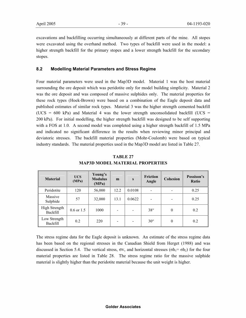
April 2005 - 39 - 04-1193-020

Golder Associates

excavations and backfilling occurring simultaneously at different parts of the mine. All stopes were excavated using the overhand method. Two types of backfill were used in the model: a higher strength backfill for the primary stopes and a lower strength backfill for the secondary stopes.

8.2 Modelling Material Parameters and Stress Regime

Four material parameters were used in the Map3D model. Material 1 was the host material surrounding the ore deposit which was peridotite only for model building simplicity. Material 2 was the ore deposit and was composed of massive sulphides only. The material properties for these rock types (Hoek-Brown) were based on a combination of the Eagle deposit data and published estimates of similar rock types. Material 3 was the higher strength cemented backfill (UCS = 600 kPa) and Material 4 was the lower strength unconsolidated backfill (UCS = 200 kPa). For initial modelling, the higher strength backfill was designed to be self supporting with a FOS at 1.0. A second model was completed using a higher strength backfill of 1.5 MPa and indicated no significant difference in the results when reviewing minor principal and deviatoric stresses. The backfill material properties (Mohr-Coulomb) were based on typical industry standards. The material properties used in the Map3D model are listed in Table 27.

TABLE 27 MAP3D MODEL MATERIAL PROPERTIES

Material UCS (MPa)

Young’s Modulus

(MPa) m s Friction

Angle Cohesion Possison’s Ratio

Peridotite 120 56,000 12.2 0.0108 - - 0.25 Massive Sulphide 57 32,000 13.1 0.0622 - - 0.25

High Strength Backfill 0.6 or 1.5 1000 - - 38° 0 0.2

Low Strength Backfill 0.2 220 - - 30° 0 0.2

The stress regime data for the Eagle deposit is unknown. An estimate of the stress regime data has been based on the regional stresses in the Canadian Shield from Herget (1988) and was discussed in Section 5.4. The vertical stress, σv, and horizontal stresses (σh1= σh2) for the four material properties are listed in Table 28. The stress regime ratio for the massive sulphide material is slightly higher than the peridotite material because the unit weight is higher.

April 2005 - 40 - 04-1193-020

Golder Associates

TABLE 28 MAP3D MODEL STRESS REGIME PROPERTIES

Material σv (MPa/m)

σh1 (MPa/m)

σh2 (MPa/m)

Peridotite 0.027 0.054 0.054 Massive Sulphide 0.030 0.060 0.060

High Strength Rockfill 0.020 0.020 0.020 Low Strength Rockfill 0.027 0.027 0.027

The stress regime data for the backfill material is based on weight of the material.

8.3 Modelling Results

Four stress analysis grids were used to review the Map3D model results. Grid 1 was oriented east-west through the centre of the deposit and Grid 2 was orientated north-south through secondary stope panels (Panel 6). Grids 3 and 4 were horizontal planes at the 252 m and 310 m elevations. An isometric view of the stress analysis grid planes and the Map3D model are illustrated on Figure 31.

Two types of stress data were reviewed in the Map3D model: minor principal stress (σ3) and deviatoric stress (σ1- σ3).

8.3.1 Minor Principal Stress

Minor principal stress results were reviewed for the proposed mining sequence in order to identify zones with low confining stress (i.e., low minor principal stress). These areas indicate zones of relaxation and, if left unsupported (i.e., backfilled), may be locations where sloughage and gravity falls can occur in the stope backs and walls. Illustrated on Figures 32 to 33 are screen captures from Grids 1 and 2 from various excavation steps. Illustrated on Figure 34 is an isometric view of the north and south walls after all the stope panels have been mined and backfilled (step 27). The minor principal results from the Map3D model indicated the following:

• Minor σ3 < 0 contours begin to occur in the walls and the back of the primary stopes after a primary stope is mined over a backfilled primary stope (steps 11-13 – Figure 32). The depth of the σ3 < 0 contours were 3-5 m into the back and the east and west walls;

• Minor to Intermediate σ3 < 0 contours begin to occur in the perimeter east and west walls of the deposit after the adjacent stope panels are removed (steps 16-17– Figure 31). The depth of the σ3 < 0 contours was 5-10 m in the west wall (between 220 m and 320 m elevations) to step 27 and 30-40 m in the east wall (between the 270 m to 320 m elevations) between

April 2005 - 41 - 04-1193-020

Golder Associates

steps 17 to 27. At step 16, thirty-two of the fifty stopes have been mined and are all below the 260 m Level; and

• Major σ3 < 0 contours occur in the north wall after step 17 (see Figure 33) and increase into the north and south walls between steps 19 and 27. Initial σ3 < 0 contour depths in the north wall were 10 m at step 14 and increase to 20-45 m between steps 19 and 27 (210 m to 350 m elevations). σ3 < 0 contour depths in the south wall were 10 m or less to step 19 and increased to 10-45 m between steps 20 and 27 (270 m to 370 m elevations).

The low confinement zones identified in the modelling indicate that there is a potential for sloughage and gravity falls around the perimeter of the deposit, particularly in the upper east and west walls (220 m to 320 m elevations) and in the north and south walls between the 210 m and 370 m elevations. These low confining zones begin to develop and increase after the majority of the mining is completed below the 260 m elevation. Backfilling the stopes and applying ground support to the perimeter walls will minimize potential sliding and ground fall instabilities.

8.3.2 Deviatoric Stress Results

Deviatoric stress (σ1-σ3) results were reviewed for the proposed mining sequence in order to identify potential failure zones. Two thresholds were generally considered: deviatoric stress of approximately 0.3 UCS (intact rock mass) when the rock mass may begin to yield and approximately 0.6 UCS (intact rock mass) when the yielded rock mass may be sufficiently yielded to begin sloughing.

The UCS values of the host rock have been estimated to be 120 MPa (peridotite) and 57 MPa for the ore (massive sulphides). Semi-massive sulphides were not included in the model but occur in the ore zone and have a UCS equal to 111 MPa. Therefore, the rock mass may begin to yield between 17 MPa (massive sulphides) and 36 MPa (peridotite) and begin to slough between 34 MPa (massive sulphides) and 72 MPa (peridotite) depending on the rock type. These thresholds need to be calibrated to field conditions when the mine is being developed.

Illustrated on Figure 35 are the deviatoric stress contours for the north and south walls of the Map3D model. Typical deviatoric stress contours values to a depth of 10-20 m into the north and south wall were between 18 MPa and 30 MPa when all stopes have been excavated in the model (step 27). A small concentration of deviatoric stress contours above 42 MPa is predicted in the centre of the south wall at the 252 m elevation.

The deviatoric stress results from the Map3D modelling indicate that some of the rock mass may yield around the perimeter of the deposit in the north and south walls. The effect of deviatoric stress will be governed by the in situ stress regime and rock mass properties. Both of these parameters have been estimated based on values from other mine sites. Therefore, even though

April 2005 - 42 - 04-1193-020

Golder Associates

major deviatoric stress issues are not expected, it would be pertinent to revisit this issue again once more information is available when the project proceeds underground.

8.4 Mining Sequence Discussion

The current mining sequence proposed for the Eagle deposit does not indicate major rock mechanics issues. The following observations have been identified from the data provided:

• The sequence considers that all full sized (i.e., 20 m strike length by 30 m high) secondary stope panels are mined only after the primary stopes on either side are filled;

• Mining begins at the 140 m elevation (i.e., Level 8 – see Figure 30) and works upward;

• A typical mining extraction cycle consists of three stope panels (primary or secondary) open and one stope panel filled. No more than three stope panels are open at one time during the total extraction sequence;

• The three stope panels open at one time are spread over two or three levels; and

• The first full sized secondary stope panel (Panel 0706 – see Figure 30) is extracted when approximately 70% of the primary panels are excavated and filled. These primary panels are located below the 260 m elevation (i.e., Levels 5 through 8).

This approach is reasonable from a rock mechanics perspective and balances production requirements and allows for flexibility. A sequencing question was raised with the regards to mining primaries concurrently on both sides of secondaries. Although not ideal, this is likely achievable with attention to local geologic conditions (rock mass quality and structure) and with controlled blasting techniques (to reduce blast vibrations). While concurrent mining is acknowledged, it is recommended that the production from these stopes be staggered as much as practical. This will minimize unfavourable interactions due to stress and blasting, while also allowing timely filling of the first production should instabilities be encountered.

April 2005 - 43 - 04-1193-020

Golder Associates

9.0 HYDROGEOLOGY

A detailed hydrogeology study of the bedrock and shallow overburden groundwater has been undertaken by the Golder Calgary office (in Alberta, Canada) and a draft study report has been issued to Warner, Norcross and Judd, and also to Kennecott Minerals Company in Marcotte, Michigan. The draft report is dated November 2004, and covers the work completed to date by Golder.

The objectives of the study were to characterize the hydraulic properties of the bedrock at six selected cored borehole locations, evaluate the hydraulic communication between the overburden and bedrock aquifer, and to estimate mine inflows for an idealized tunnel.

Six existing representative NQ-cored boreholes were selected for further testing, to cover the reported lithology and a range in orientations and inclinations. Geophysical and flow logging was performed to identify localized zones of elevated hydraulic conductivity. Hydraulic testing was subsequently carried out on zones of interest using packer testing methods. Based on the results, a conceptual model of the groundwater system was developed, and groundwater inflows into an idealized mine were estimated.

The study determined that the uppermost 300 feet of the tested rock mass is weathered, and the hydraulic conductivity was determined to be on the order of 2E-6 cm/s. The underlying rock (to a depth of 1,000 ft) exhibited a lower hydraulic conductivity, on the order of 5E-8 cm/s. Monitoring of the overburden aquifer suggests that there is negligible hydraulic communication between the overburden aquifer and the bedrock mass.

Some mine inflow estimates for the project have been developed. However, additional analysis is being performed to refine inflow estimates to account for any bias of the borehole orientation and dip relative to the dominant fracture patterns. This analysis is being completed in January, and the conceptual model and inflow estimates will be revised.

The study data generated as part of this report has been conducted on a scale that should be adequate to make estimates of parameters at a prefeasibility level.

April 2005 - 44 - 04-1193-020

Golder Associates

10.0 CLOSURE

We trust that this report meets your needs at the present time. Should you have any questions, please do not hesitate to contact the undersigned.

GOLDER ASSOCIATES LTD.

Paul Palmer, P.Eng. Geological Engineer

K.J. Beauchamp, P.Eng. Associate

PP/KJB/lb

FIGURE ___Fi

le L

ocat

ion:

S:\A

ctiv

e\20

04\1

190_

Sud

bury

\119

3\04

-119

3-02

0 K

enne

cott

Eag

le G

eote

chM

ichi

gan

DATE JAN 2005PROJECT 04-1193-020

DRAWN…TVCHKD…PP

Eagle Deposit Site Plan 1

Taken from: Eagle Nickel Project – Scoping Study Report, AMEC 2004

FIGURE 2P

roje

ct:

04-1

193-

020

Dra

wn:

R

evie

wed

: ___

__


DRAWN……….CHKD…KJB…

Eagle Deposit: Isometeric View of Geotechnical Drillhole Coverage

3. Hangingwall

1. Crown

4. Eastern Zone

2. Footwall

5. Decline and Portal Ramp

E

FIGU

RE ___ DATE: JANUARY 2005

PROJECT: 04-1193-020DRAWN…...CHKD……

TVPP

Plan: RQD and RMR Contouring for 405 Elev.

3

5177550

5177590

4314

00

4314

40

Intrusive Envelope

RQD

5177550

5177590

4314

00

4314

40

Intrusive Envelope

RMRN

E

Top of Bedrock

Contoured Plane

Intrusive Envelope

Decline

Portal Ramp

“Fault”

“Fault”

FIGU



TVPP


4

RQD

Intrusive Envelope

5177410

5177430Vent Raise

RMR

Intrusive Envelope

5177410

517743043

1420

4314

00

Vent Raise

Incline Incline

E

Top of Bedrock

Contoured Plane

Intrusive Envelope

Decline

N

4314

20

4314

00

“Fault”

“Fault”

FIGU



TVPP


5

E

Top of Bedrock

Contoured Plane

Intrusive Envelope

Decline

RQD

Intrusive Envelope

5177450

5177470

4314

20

4314

00

Internal Ramp

RMR

Intrusive Envelope

5177450

5177470

4314

20

4314

00

Internal Ramp

N

“Fault”

“Fault”

FIGU



TVPP


6

E

Contoured Plane

Intrusive Envelope

RQD

Intrusive Envelope

5177470

5177490

4314

20

4314

40

Internal Ramp

RMR

Intrusive Envelope

5177470

5177490

4314

20

4314

40

Internal Ramp

Top of Bedrock

Decline

N

“Fault”

“Fault”

FIGU



TVPP


7

E

Contoured Plane

Intrusive Envelope

Top of Bedrock

Decline

N

RQD

Intrusive Envelope

5177510

5177530

4314

20

4314

40

Internal Ramp

RMR

Intrusive Envelope

5177510

5177530

4314

20

4314

40

Internal Ramp

“Fault”

“Fault”

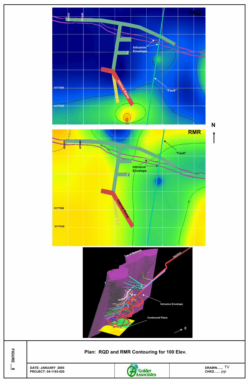
FIGU



TVPP


8

E

Contoured Plane

Intrusive Envelope

Top of Bedrock

Decline

4314

20

4314

40 RQD

Intrusive Envelope

Internal Ramp

RMR

Intrusive Envelope

4314

20

4314

40

Internal Ramp

5177530

5177550

5177530

5177550

N

“Fault”

“Fault”

FIGU



TVPP

Traverse Section: RQD and RMR Contouring for 431420E Facing East

9

RQD

Intrusive Envelope

360 Elv.

220 Elv.

120 Elv.

5177

400

Internal Ramp

5177

440

Internal Ramp

Intrusive Envelope

Decline

RMR

Intrusive Envelope

360 Elv.

220 Elv.

120 Elv.

5177

400

Internal Ramp

5177

440

E

FIGU



TVPP


10

RQD

Intrusive Envelope

360 Elv.

220 Elv.

120 Elv.

5177

400

Internal Ramp

5177

440

Internal Ramp

Intrusive Envelope

Decline

RMR

Intrusive Envelope

360 Elv.

220 Elv.

120 Elv.

5177

400

5177

440

E

Internal Ramp

Incline Incline

FIGU



TVPP


11

RQD

Intrusive Envelope

360 Elv.

220 Elv.

120 Elv.

5177

400

Internal Ramp

5177

440

Internal Ramp

Intrusive Envelope

Decline

E

Incline

Vent

Rai

se

RMR

Intrusive Envelope

360 Elv.

220 Elv.

120 Elv.

5177

400

Internal Ramp

5177

440

Incline

Vent

Rai

se

FIGU



TVPP


12

RQD

Intrusive Envelope

360 Elv.

220 Elv.

120 Elv.

5177

400

Internal Ramp

5177

440

Internal Ramp

Intrusive Envelope

Decline

Incline

E

Incline

RMR

Intrusive Envelope

360 Elv.

220 Elv.

120 Elv.

5177

400

Internal Ramp

5177

440

Incline

FIGU



TVPP


13

RQD

Intrusive Envelope

360 Elv.

220 Elv.

120 Elv.

5177

400

Internal Ramp

5177

440

Internal Ramp

Intrusive Envelope

Decline

Incline

E

Incline

RMR

Intrusive Envelope

360 Elv.

220 Elv.

120 Elv.

5177

400

5177

440

Incline

Internal Ramp

FIGU



TVPP

Longitudinal Section: RQD and RMR Contouring for 5177500N Facing North

14

N

Contoured Plane

Intrusive Envelope

RQD

300m Elv.

200m Elv.

100m Elv.

4315

00

4314

40

400m Elv. RMR

300m Elv.

200m Elv.

100m Elv.

4315

00

4314

40

400m Elv.

Decline

Bedrock

“Fault”

“Fault”

FIGU



TVPP

Longitudinal Section: RQD and RMR Contouring for 5177560N Facing North

15

N

Contoured Plane

Intrusive Envelope

4314

20

4314

40 RQD

300m Elv.

200m Elv.

100m Elv.

4315

00

4314

40

400m Elv.

Decline

Bedrock

RMR

300m Elv.

200m Elv.

100m Elv.

4315

00

4314

40

400m Elv.

“Fault”

“Fault”

FIGURE ___P

roje

ct: 0

4-11

93-0

20…

……

….

Dra

wn:

TV

R

evie

wed

: PP

Rev

.: …

……

……

FILE

LO

CA

TIO

N …

……

……

…8.

5x11

Fig

-por

t.ppt

DATE January 11, 2005PROJECT 04-1193-020

DRAWN……….CHKD……

TVPP

MAJOR DISCONTINUITY SETS (ALL FEATURES) SEMI-MASSIVE SUPHIDE AND MASSIVE SUPHIDE 16

FIGURE ___P

roje

ct: 0

4-11

93-0

20…

……

….

Dra

wn:

TV

R

evie

wed

: PP

Rev

.: …

……

……

FILE

LO

CA

TIO

N …

……

……

…8.

5x11

Fig

-por

t.ppt



TVPP

MAJOR DISCONTINUITY SETS (ALL FEATURES) PERIDOTITE AND FELDSPAR PERIDOTITE 17

FIGURE ___P

roje

ct: 0

4-11

93-0

20…

……

….

Dra

wn:

TV

R

evie

wed

: PP

Rev

.: …

……

……

FILE

LO

CA

TIO

N …

……

……

…8.

5x11

Fig

-por

t.ppt



TVPP

MAJOR DISCONTINUITY SETS (ALL FEATURES)SANDSTONE AND SILTSTONE 18

FIGURE 21P

roje

ct:

04-1

193-

016

Dra

wn:

PG

PR

evie

wed

: ___

__Fi

le L

ocat

ion:

N:\a

ctiv

e\20

04\1

193\

04-1

193-

016\



PGP

UNWEDGE ASSESSMENT 5 m HIGH BY 5.0 m WIDE

75° Orientation 90° Orientation 105° Orientation

MAXIMUM WEIGHT vs ORIENTATION SUPPORT PRESSURE vs ORIENTATION

T/m2

0

20

40

60

80

100

120

140

160

180

200

0 10 20 30 40 50 60 70 80 90 100 110 120 130 140 150 160 170 180

Max

. Wed

ge W

eigh

t

Possible Tunnel Axis Trend

Optimization for Tunnel Axis Plunge = 0°

Current Tunnel Axis Trend = 15°

0

1

2

3

4

0 10 20 30 40 50 60 70 80 90 100 110 120 130 140 150 160 170 180

Pres

sure

for F

S=1.

300




FIGURE 22P

roje

ct:

04-1

193-

016

Dra

wn:

PG

PR

evie

wed

: ___

__Fi

le L

ocat

ion:

N:\a

ctiv

e\20

04\1

193\

04-1

193-

016\



PGP

UNWEDGE ASSESSMENT 5m HIGH BY 6.2 m WIDE (INTERSECTIONS)

0

100

200

300

400

0 10 20 30 40 50 60 70 80 90 100 110 120 130 140 150 160 170 180

Max

. Wed

ge W

eigh

t




0.0

0.1

0.2

0.3

0.4

0.5

0.6

0.7

0.8

0 10 20 30 40 50 60 70 80 90 100 110 120 130 140 150 160 170 180

Pres

sure

for F

S=1.

300





MAXIMUM WEIGHT vs ORIENTATION SUPPORT PRESSURE vs ORIENTATION

T/m2

FIGURE 23P

roje

ct:

04-1

193-

016

Dra

wn:

PG

PR

evie

wed

: ___

__Fi

le L

ocat

ion:

N:\a

ctiv

e\20

04\1

193\

04-1

193-

016\



PGP

UNWEDGE ASSESSMENT 4.7m HIGH BY 8.0 m AND 8.8 m WIDE (INTERSECTION)

0

100

200

300

400

500

600

700

800

0 10 20 30 40 50 60 70 80 90 100 110 120 130 140 150 160 170 180

Max

. Wed

ge W

eigh

t




0

100

200

300

400

500

600

700

800

900

1000

1100

0 10 20 30 40 50 60 70 80 90 100 110 120 130 140 150 160 170 180

Max

. Wed

ge W

eigh

t





MAXIMUM WEIGHT vs ORIENTATION (4.7m BY 8.0m)

30 0rient

90° Orientation

MAXIMUM WEIGHT vs ORIENTATION (4.7m BY 8.8m)

FIGURE 24P

roje

ct:

04-1

193-

016

Dra

wn:

PG

PR

evie

wed

: ___

__Fi

le L

ocat

ion:

N:\a

ctiv

e\20

04\1

193\

04-1

193-

016\

DATE APRIL 2005PROJECT 04-1193-020


PGP

TRANSVERSE AND LONGITUDINAL LONGHOLESTOPE FACE STABILITY PLOT

Mathews Graph (Side Wall)

0.1

1

10

100

1000

0 5 10 15 20 25

Hydraulic Radius, HR

Stab

ility

Num

ber,

N' Transverse

LongitudinalQ=8.0 (Trans)Q=3.0 (Trans)10% Dilution20 % DilutoinLargest Stope (Trans)

Stable ZoneUnsupported Transition Zone

Caved Zone

Stable with Support

Supported Transition Zone

FIGURE 25P

roje

ct:

04-1

193-

016

Dra

wn:

PG

PR

evie

wed

: ___

__Fi

le L

ocat

ion:

N:\a

ctiv

e\20

04\1

193\

04-1

193-

016\



PGP

TRANSVERSE AND LONGITUDINAL LONGHOLEEND WALLS STABILITY PLOT

Mathews Graph (End Walls)

0.1

1

10

100

1000

0 5 10 15 20 25

Hydraulic Radius

Stab

ility

Num

ber,

N' Longitudinal

TransverseQ=3.0 (Trans)Q=0.2 (Trans)10% Dilution20% DilutionLargest Stope (Trans)

Stable ZoneUnsupported Transition Zone

Caved Zone

Stable with Support


FIGURE 26P

roje

ct:

04-1

193-

016

Dra

wn:

PG

PR

evie

wed

: ___

__Fi

le L

ocat

ion:

N:\a

ctiv

e\20

04\1

193\

04-1

193-

016\



PGP

TRANSVERSE AND LONGITUDINAL LONGHOLESTOPE BACK STABILITY PLOT

Mathews Graph (Back)

0.1

1

10

100

1000

0 5 10 15 20 25

Hydraulic Radius

Stab

ility

Num

ber,

N' Q=19.5 (Trans)

Q=3.0 (Trans)LongitudinalTransverse10% Dilution20% DilutionLargest Stope (Trans)

Stable Zone Unsupported Transition Zone

Caved Zone

Stable with Support


FIGURE 28P

roje

ct:

04-1

193-

016

Dra

wn:

R

evie

wed

: ___

__Fi

le L

ocat

ion:

N:\a

ctiv

e\20

04\1

193\

04-1

193-

016\

APRIL 2005PROJECT 04-1193-020

DRAWN...DJC..CHKD…KJB…

Cs VERSUS QEquiv FOR THE SCALED SPAN ASSESSMENTS EAGLE CROWN PILLAR

0.1

1.0

10.0

100.00.001 0.010 0.100 1.000 10.000 100.000 1000.000

NGI - Rock Quality Index, Q

Sca

led

Crow

n P

illar

, Cs

(m)

Hw/FwFailedOreFilledStability LinePanlel 0106 RMR=85Panel 0106 RMR=75Panels 0106 and 0107 RMR=85Panels 0106 and 0107 RMR=75Panels 0106, 0107 and 0108 RMR=85Panels 0106, 0107 and 0108 RMR=75No Panels Level 1 RMR=85No Panels Level 1 RMR=75Initial Assessment RMR=85Initial Assessment RMR=75

UNSTABLE

FIGURE 29P

roje

ct:

04-1

193-

016

Dra

wn:

R

evie

wed

: ___

__Fi

le L

ocat

ion:

N:\a

ctiv

e\20

04\1

193\

04-1

193-

016\


DRAWN...DJC..CHKD…KJB…

CPILLAR OUTPUT FOR THE EAGLE CROWN PILLAR ASSESSMENTS

FigureEAGLE DEPOSITMAP3D MODEL – STOPE LABELLING AND SEQUENCING

VIEW - SOUTH30

0106 0107 0111011001090108

0206 0207 0208

0306 0307 0308 0309

0706

0606

0506

0406

0707

0607

0507

0407

0708

0608

0508

0408

0808 0809

0709

0609

0509

0409

0310

0410

0810

0710

0610

0510

0405

0705

0605

05050504

0604

0704

0503

0603

0703

0502

0602

0702

0501

Massive Sulphide

Level

1

2

3

8

7

6

5

4

Panel 1 2 3 4 5 6 7 8 9 10 11

0510

05 = Level

10 = Panel

Note:All odd Panel #’s are primary stopes

Pro

ject

: 05-

1193

-003

……

……

.D

raw

n: D

FLR

evie

wed

: _P

GP

____

Rev

.: …

……

……

FILE

LO

CAT

ION

……

……

……

11x

17.5

Fig

-por

t.ppt

FIGURE 31P

roje

ct: 0

4-11

93-0

20…

……

….

Dra

wn:

DFL

Rev

iew

ed: _

PG

P__

__R

ev.:

……

……

…FI

LE L

OC

ATI

ON

……

……

……

8.5

x11

Fig-

port.

ppt

DATE MARCH, 2005PROJECT 04-1193-020


DFLPGP

EAGLE PROJECT – MAP3D MODEL – ISOMETRIC VIEW

N

Grid 2

Grid 1

- PRIMARY PANELS

- SECONDARY PANELS

GRID 3(310m)

GRID 4(252m)

440m

140m

FigureEAGLE PROJECT – MAP3D – SIGMA 3 RESULTSGRID 1 – STEPS 11, 13, 16, 20, 23 ,27

VIEW - SOUTH32

Pro

ject

: 04-

1193

-020

……

……

.D

raw

n: D

FLR

evie

wed

: _P

GP

____

Rev

.: …

……

……

FILE

LO

CAT

ION

……

……

……

11x

17.5

Fig

-por

t.ppt

GRID 1 – STEP 11 GRID 1 – STEP 23


GRID 1 – STEP 16

GRID 1 – STEP 20

380 L

360 L

340 L

320 L

300 L

280 L

260 L

240 L

220 L

360 L

340 L

320 L

300 L

280 L

260 L

240 L

220 L

200 L

180 L

0501

0603

0405

360 L

340 L

320 L

300 L

280 L

260 L

240 L

220 L

200 L

180 L

0503 0507

0706

360 L

340 L

320 L

300 L

280 L

260 L

240 L

220 L

200 L

180 L

0409

0502

0608

360 L

340 L

320 L

300 L

280 L

260 L

240 L

220 L

200 L

0207

0408

380 L

360 L

340 L

320 L

300 L

280 L

260 L

240 L

220 L

0109

0206

Surface = 440m

380 L

180 L

380 L

LOW SIGMA 3

CONTOURS

EAST WEST EAST WEST EAST WEST

EAST WEST EAST WEST EAST WEST

LOW SIGMA 3

CONTOURS

STOPE OUTLINES

LOW SIGMA 3

CONTOURS

LOW SIGMA 3

CONTOURS

Figure

GRID 2 – STEP 13

EAGLE PROJECT – MAP3D –SIGMA 3 RESULTS – SECONDARY PANELSGRID 2 – STEPS 11, 13, 14 ,17, 19 ,27

VIEW - WEST33

Pro

ject

: 04-

1193

-020

……

……

.D

raw

n: D

FLR

evie

wed

: _P

GP

____

Rev

.: …

……

……

FILE

LO

CAT

ION

……

……

……

11x

17.5

Fig

-por

t.ppt


GRID 2 – STEP 27

GRID 2 – STEP 14

GRID 2 – STEP 17

0706

0206

180 L

380 L

180 L

180 L

360 L 360 L

380 L

180 L

360 L

Surface = 440m

NORTHSOUTH

NORTHSOUTH NORTHSOUTH

NORTHSOUTHNORTHSOUTH

NORTHSOUTH

LOW SIGMA 3

CONTOURS

LOW SIGMA 3

CONTOURS

LOW SIGMA 3

CONTOURS

LOW SIGMA 3

CONTOURS

LOW SIGMA 3

CONTOURS320 L

220 L

180 L

FigureEAGLE PROJECT – MAP3D – SIGMA 3 RESULTSGRID 1,2,3 AND 4

NORTH AND SOUTH WALL34

Pro

ject

: 04-

1193

-020

……

……

.D

raw

n: D

FLR

evie

wed

: _P

GP

____

Rev

.: …

……

……

FILE

LO

CAT

ION

……

……

……

11x

17.5

Fig

-por

t.ppt

NORTH WALL – STEP 27 SOUTH WALL – STEP 27

N

N

440m

310m

252m

LOW SIGMA 3

CONTOURS

LOW SIGMA 3

CONTOURS

252m

310m

440m

FigureEAGLE PROJECT – MAP3D –DEVIATORIC STRESS RESULTSGRID 1,2,3 AND 4

NORTH AND SOUTH WALL35

Pro

ject

: 04-

1193

-020

……

……

.D

raw

n: D

FLR

evie

wed

: _P

GP

____

Rev

.: …

……

……

FILE

LO

CAT

ION

……

……

……

11x

17.5

Fig

-por

t.ppt

NORTH WALL – STEP 27 SOUTH WALL – STEP 27

N

N

440m

310m

252m

DEVIATORIC STRESS CONTOURS

BETWEEN 18-36 MPa

440m

310m

310m

DEVIATORIC STRESS CONTOURS > 42MPa

APPENDIX A

LITHOLOGICAL SECTIONS A1 TO A12

FIGURE A1P

roje

ct:

04-1

193-

016

Dra

wn:

PG

PR

evie

wed

: ___

__Fi

le L

ocat

ion:

N:\a

ctiv

e\20

04\1

193\

04-1

193-

016\



PGP

LITHOLOGY – LEVEL 405

FIGURE A2P

roje

ct:

04-1

193-

016

Dra

wn:

PG

PR

evie

wed

: ___

__Fi

le L

ocat

ion:

N:\a

ctiv

e\20

04\1

193\

04-1

193-

016\



PGP


FIGURE A3P

roje

ct:

04-1

193-

016

Dra

wn:

PG

PR

evie

wed

: ___

__Fi

le L

ocat

ion:

N:\a

ctiv

e\20

04\1

193\

04-1

193-

016\



PGP


30 0rient

FIGURE A4P

roje

ct:

04-1

193-

016

Dra

wn:

PG

PR

evie

wed

: ___

__Fi

le L

ocat

ion:

N:\a

ctiv

e\20

04\1

193\

04-1

193-

016\



PGP


FIGURE A5P

roje

ct:

04-1

193-

016

Dra

wn:

PG

PR

evie

wed

: ___

__Fi

le L

ocat

ion:

N:\a

ctiv

e\20

04\1

193\

04-1

193-

016\



PGP


FIGURE A6P

roje

ct:

04-1

193-

016

Dra

wn:

PG

PR

evie

wed

: ___

__Fi

le L

ocat

ion:

N:\a

ctiv

e\20

04\1

193\

04-1

193-

016\



PGP


FIGURE A7P

roje

ct:

04-1

193-

016

Dra

wn:

PG

PR

evie

wed

: ___

__Fi

le L

ocat

ion:

N:\a

ctiv

e\20

04\1

193\

04-1

193-

016\



PGP

LITHOLOGY – SECTION 431420E

FIGURE A8P

roje

ct:

04-1

193-

016

Dra

wn:

PG

PR

evie

wed

: ___

__Fi

le L

ocat

ion:

N:\a

ctiv

e\20

04\1

193\

04-1

193-

016\



PGP


FIGURE A9P

roje

ct:

04-1

193-

016

Dra

wn:

PG

PR

evie

wed

: ___

__Fi

le L

ocat

ion:

N:\a

ctiv

e\20

04\1

193\

04-1

193-

016\



PGP


FIGURE A10P

roje

ct:

04-1

193-

016

Dra

wn:

PG

PR

evie

wed

: ___

__Fi

le L

ocat

ion:

N:\a

ctiv

e\20

04\1

193\

04-1

193-

016\



PGP


FIGURE A11P

roje

ct:

04-1

193-

016

Dra

wn:

PG

PR

evie

wed

: ___

__Fi

le L

ocat

ion:

N:\a

ctiv

e\20

04\1

193\

04-1

193-

016\



PGP


FIGURE A12P

roje

ct:

04-1

193-

016

Dra

wn:

PG

PR

evie

wed

: ___

__Fi

le L

ocat

ion:

N:\a

ctiv

e\20

04\1

193\

04-1

193-

016\



PGP

LITHOLOGY – SECTION 5177560N

APPENDIX B

ROCK MASS CLASSIFICATION SYSTEMS (EXCERPTS FROM PREDICTION AND UNCERTAINTIES IN

GEOLOGICAL ENGINEERING AND ROCK MASS CHARACTERIZATION ASSESSMENTS -

T.G. CARTER, 1992. PP 1-9 TO 1-12)

1-9

situationanormal sheartestmay be sufficiently usefulto allow usually representativeonly of thebetter rock. Thus again thisrepresentativedatato becollected. Howeversuchtestsmaynot sampling process, of itself introducessome further level ofbe suited to the determination of the stress-displacement uncertaintyinto thedata-base.behaviourof discontinuities isolating a rock block that maypotentially slide or fall from the periphery of an undergroundexcavation(Figure 12 lower right diagram). In theformercase Severalrockmassclassificationsystemshavebeendeveloped,dilation is permitted to occur freely, but in the latter ~ specifically in an attempt to quantify precedentexperience;dilation may be inhibited by surrounding rock such that the however,by their very formulation they provide a meansfornormalstressmayincreasewith sheardisplacement.In this case rationalizingsomeof the vaguariesin basicrockmasspropertynornmi compressivestress- displacementbehaviouris highly definition. Typical of theseclassificationsarethosepublishedbynon-linear and at high values of normal stress o~, closure Bieniawski (1973, 1976)andby Bartonand co-workers(1974).becomesasymptoticto the originalapertureof thediscontinuity. These empirical methods of design, which are based onAccurately determining realistic ranges for shear strength observationsof rock mass and support behaviourin similarpropertiesthusdemandsconsiderableattentionto detail, notonly situationswere essentiallydevelopedfor usein civil excavationsin the laboratorybut alsoin describingdiscontinuity surfacesin where geometryis typically much simpler than in most minethefield. layouts. Due carethereforemust betakenwhenapplying them

to excavationdesign for mining applications. In consequenceThe precisecontrol on shearstrengthof aperture,is difficult severalmodified schemeshavebeenspecifically developedfor

to evaluate. Largeaperturescanresultfrom sheardisplacement mining use,namelythoseby Mathewset al. (1981)Potvinet. alofdiscontinuitieshavingappreciableroughness,fromoutwashof (1989)andby Laubscher(1977).filling materials(e.g. clay), or from solution or from tensileopening of the fracture. In most subsurfacerock masses,apertureswill be small, usually well lessthanhalfa millimetre, Despitethe fact thatmanysimplifying assumptionsexist withbut actualvalueswill be difficult, if not impossible,to measure theuseof classificationapproaches,it is generallyacceptedthatalthoughestimatesscanbe madethroughmeasurementsof the these, essentiallyempirical design methods provide a goodpermeabilityor hydraulicconductivityof thediscontinuity within starting point for supportdesign. They are, however, only astherockmass. reliable as the assessmentof the basic parameters. Sound

engineeringjudgementmust still be usedin selectingthe inputThis measurementandhencetheinfluenceofaperturemayalso parameters,bearing in mind the uncertaintiesin the raw data

be subject to further error due to the fact that many discussedpreviously. Whenreliable representativenesscan bediscontinuities contain full or partial filling comprising, for assuredfrom detailed evaluationof uncertaintiesin input data,examplecalcite,chlorite, clay, silt, fault gouge,breccia,quartz thesemethodsof assessmentaremost useful. For preliminaryor other minerals. Suchfilling mayalsothereforeexertamajor design,when only limited geotechnicaldata is available,theseinfluence on shear strength. With the exception of those rockmassclassificationsystemsthemselvesprovideaconvenientdiscontinuitiesfilled with relativelystrongveinmaterials(calcite, way of comparingdifferentrockmassconditionsacrossa site.quartz, pyrite), filled joints will generally have lower shearstrengths than comparable clean, closed discontinuities.However,again,althoughthebehaviourof filled discontinuities, In Civil practise,Barton’sQ-systemandBieniaswki’sRMRwhich largelydependson thepropertiesof the filling materials, method are most commonly used. The mining industry byis beyondthescopeof this paper,it is importanthereto notethat contrast,generallyavoidsdirect useof either of theseschemesthe lack of a simple definition of controlling shearstrength preferringuseof modifiedschemesfor deepstopedesign,suchconstitutes yet anotherlevel of uncertainty within the basic asLaubscher’sMRMR and/ortheMathewsor Potvin’smethods.geologicaldatabasethat formsthefoundationfor anydesign. Laubscher’sMRMR system is a modification of Bieniawski’s

RMR systemwhile both theMathewsandPotvin methodsarebased on Barton’s Q. For shallow opening design, recent

3. ROCKMASS CLASSIFICATION development work has formulated a further modifiedclassificationbasedmainly on the Q system (Carter, 1992b).

Somestepstowardsquantifyingtheuncertaintiesinherentin all Parametersfor eachof thesesystemsjust like thestraightforwardof these discrete measurementscan be achievedby careful original schemes,can be estimated from surfacemappingandcomparativeclassification, from core logging information then verified as excavation

proceeds.It will be appreciated,by now that evaluatingthe controlling

strength of the rock mass that will surround a proposedexcavationor will form acutslope,on ascalethatis meaningful Although each of the classification and evaluationsystemsfor design is difficult, Laboratory tests of rock specimens differ, theyall rely on collectionof similardata. However,thereprovide data relevantonly of a very small, highly selective areminor differencesin thebasicsuite of parametersdefinedbysampleof therockmassfrom whichtheywere removed.In fact, the two principal classificationapproaches. In consequence,for most typical projects the samplestestedin the laboratory thereis advantagein applying both of the original schemesforrepresentwell less than 1 % of the volume of the rock mass classyfing the rockmassandthen comparingthededucedRMRrequiredto beevaluated.In addition,sinceonly thosespecimens andQ values. This procedurenot only providesconfirmationofwhichsurvive thecollection andpreparationprocessare te5~ed, the reliability of the field classification data, it also allowstheresults of these testsalso representa highly biasedsample, inherent rock mass variability and uncertainty in parameter

definition to bebetterdefined.

1-10

3.1 Barton’s0 System Examinationofthe termsin the Q relationshippresentedabove,is instructivein consideringuncertainty in defining rock masspropertiesaseachtermhassomephysicalsignificance.ThetermRQD/J~representsthe averageblock sizeof the mass;J,IJ. thepeakshearstrengthof controlling jointsandtheJ.a/SRiFtermtherelative importanceof water pressureand the effects of highstress, squeezing,swelling, or loosening of the rock mass.Specificparameterdescriptionsaregivenon Table2.

Table2: NGI Q-SystemParameterCodes

Bartonet al (1974)analyzedextensivedatarelatingrockmassquality to thebehaviourandsupportrequirementsofundergroundexcavations. Barton’s original work provided guidelines forevaluating the structure of the rock mass, the frictionalcharacteristics of fractures and the stressessurrounding anopening. It was basedon 212 case recordsof excavationsinigneous, metamorphicand sedimentaryrocks. Openingspansrangedfrom 5 - 30 m, and depthsrangedfrom very shallow(<50 m) to 500m. To date, hundredsof additional openingshavebeenevaluatedusing the system, which is expressedasfollows:

RQD . ___

.J~ .J~ SRF

Where:RQD = rockquality designation(Deere,1964)

= joint setnumber= joint roughnessnumber= joint alterationnumber= joint waterreductionfactor

51W = stressreductionfactor

POOR FAIRVERY EXT.

GOOD GOOD GOOD~7]

>~ ~~TITNO SUPPORT• REQIJIR 0.— —

0

ENVELOPE TOSTABLE CASERECORDSIllarton . 19741

20 (REFER TOFIGURE lBB CRITICAL

10 SCALED SPANEQUATION)

S

2

1000tO 40 100 400

ROCK MASS QUALITY (Cl

SUGGESTED DESIGN SPAN LIMITS FORVARIOUS EXCAVATION TYPES IN DIFFERENT

QUALITY ROCK MASSES

• MAN-MADE EXCAVATIONS

• NATURAL CAVERNS ATCARLSBAD NEW MEXICO

Figure13: Basic Q-System Classification ChartRelating UnsupportedSpan to Rock MassQuality

As indicatedon Figure 13, which showsplotted valuesfromBarton’soriginal databasefor unsupportedstableopenings,thevalueof Q, whichvarieslogarithmically,rangesfrom 1 for poorground to 1,000 for exceptionallygood quality rock which ispracticallyunjointed. This charthasbeenfurther extendedbyBartondownto 0.001for exceptionallypoor,squeezingground.

item and Description Parameter & value

Number of Setsof DtscontinuitiesMassiveOne setTwo setsThree setsFour or more setsCrushedrock

J,,

0.52.04.09.0i5.020.0

Rougnessof DncontsnustsesNoncontinuousjointsRough and wavySmoothand wavyRough and planarSmoothand planarSlick and planarFilled discontinuities

J,

4.03.02.0*1.5*1.0*0.5*1.0

Filling and Wail-Rock Alteration, EssentlailyUnfilledHeeledStainingonly; no alterationSilty orsandymatingsClay coatings

J 0.751.03.04.0

Filling and Wall-RockAlteration, FilledSand orcrushedreekfillingStiff clay filling lessthan5 mm thickSoft clay filling less than5 mm thickSwelling clay filling less than5 mm thickStiff clay filling more than5 mm thickSoft clay filling morethan5 mm thickSwelling clay filling morethanS mm thick

J~

4.06.08.012.010.015.020.0

Water ConditionsDryMedium water inflowLarge inflow; unfilled jointsLarge inflow; filled joints with washoutLarge I high transient inflow; filled jointsLarge I continuousinflow; filled joints

Jr

1.0

0.660.5

0.330.2 to 0.10.1 to 0.05

StressReductionClassLooserock with clay-filled discontinuitiesLooserockwith opendiacontinuitiesShallow depth(50 m or less)rockwith clay-filled discontinuitiesRockwith tight unfilled discontinuities;mediumstress

SRF

10.0S.O

2.51.0

Rock-MassQuality for TunnellingExceptionallypoorExtremelypoorvery poorPoorFairGoodvery goodExtremelygoedExceptionallygood

Q

< 0.01

0.01 to 0.100.10 to 1.00

1.00 to 4.00

4.00 to 10.010.0 to 40.0

40 to 100

100 to 400

400 to 1000

Adaptedfrom: Barton,N., Lien, R., andLunde,1., 1974* Add 1.0 if themeanjoint spacingexceeds3.0 m.

200

MN EDIATE 100

CDL LAPSE

so

-

8z

0

0

z

1-11

3.2 Bieniawski’sRMR System Variousvaluesareassignedfor theseparameteras outlinedinTable 3 below, suchthat the final adjustedRMR value canbe

The Rock Mass Rating (RMR) system was developedby ratedinto oneof 5 classeswhich describetherelativequality ofBieniawski in 1973 andmodified over subsequentyearsas the therockmass. Although intendedprimarily for evaluationwithdatabaseof casehistories increased. In its current form it is respectto mappedexposures,becauseof theprimary dependancebasedon datafrom 189 casehistories. It usessixparameters: of this classification system on intact strength and RQD

measurement,evaluationof boreholecoredatais often somewhat• Uniaxialcompressivestrengthof intactrock. easierwith this method thanwith theQ approach. Nevertheless• RQD(rockquality designation). both systemscanbereadilly comparedas the initial databaseof• Spacingof discontinuities. ill casehistoriesworldwideusedfor the RMR systemhavenot• Conditionof discontinuities. only beencorrelatedwith stand-uptime and maximum stable• Groundwaterconditions. spansfor undergroundexcavationsbut also havebeencorrelated• Orientationof discontinuities. with referenceto the Q systemcodes.

Table 3 : GeomechanicsSystemRatingValues

ClassificationParametersand Their RatingsPoint-loadstrength

Strengthof intactrock indexIssaterlal Usiaxial compressive

strength

>SMPa 4-SMPa 2-4MPa l-2MPs Useofuniaxial

compressiveteatpreferred

10-25 3-10 1-3Ml’s MN Ml’s

<200MN 100-200MN 50-100MN 25-50Ml’s

Rating 15 12 7 4 2 1 0

Drill corequslity-RQDRating

90-100% 75-90% 50-75% 25-50% 25%20 17 13 3

SpacingofinistsRating

>3m 1-3m 0.3-im SD-SOOmm <50mm50 25 20 10 5

Cosditionsofjoints

veryroaghsurfaces;net

continuous;noseparation;hsrdjoint wall rock

Slightly roaghssrfaces;sepsrati

on<1mm;hardjointwall rock

Slightly rosghsurfaces;

separation<1mm;soft jointwall rock

Slickensidedsurfaces

orgouge<Soonthickorjointsopenshout 1-5mm; continuousjoints

Soft gouge>5 mm thick

orjoints open>5mm;

continsossjoints

Rating 25 20 12 6 0

Groundwater

Inflowper 10 mtunnel length

JointWaterpressure

Ratio Majorprincipalstress

None 25 LIens 25-125L/min >125Llmin

0 0.0-0.2 0.2-0,5 >0.5

Generalconditions Completelydry Moist only Waterundermoderatepressure

Severewaterprohlems

Rating 10 7 4 0

Adjustments For Joint OsientationStrike anddiporientationsofjoints

veryfavosrahle Favourahle Ear Unfavourable

veryunfavourable

0Tassels

I__Foundations j~ 0Ratings Slopes 0

10 -12

7 IS -2525 50 -~

Rock Mass ClassesAnd Their Ratings

77~7~]~77777ClsasNo Ill iv vDescription ~ Fairrock Poorrock v.l’oor rock

Rating ~ 50-70 2550 25

Meaning of Rock Mass Classes

ClassNo I 11 III lv vAveragestand-aptime 10 yearsfor

Smapan6 monthsfor

4mspanI weekforimapan

5 hr forISmapan

10 misforOsmapan

Cohesionof the rockmass 300 kPa 200-300kPa 150-200kPa l00- 150kPa 100 kPa

Rockmass friction angle 45’ 40-45’ 35-40’ 30-35’ 50’

Caveahilityof ore verypoor Will not ravereadily; largefragments

Fair Will cavereadily;goodfragmentation

very good

1-12

The correlationrelationship first proposedby Bieniawski greaterthe potential for maintaining thepresenceof unopened(1976)andwhichhasbeenwidely appliedandfoundto fit most or marginallyhealeddiscontinuities. For instance,H-series,situations,is as follows: (100mmdiameter)core of a particularRQDmay representan

RMR = 9 In Q + artificially higher numberthan would havebeenobtainedforNX core. Conversely,verysmallcorewouldtendto reducetheor calculatedvalue. Heuze,1971andGoodman,1976 indicatethat

‘RMR ~ to maintain similar RQD valuesas would be measuredon N-Q = ~I., I I sized core, thereferencelength should bealtered for different

\9 ) core diameters, such that the referencelength would bemaintainedat abouttwicethecorediameter,asillustratedby thedataplotted on Figure 14.

Deere andDeere, 1989 confirmed Heuze’sindications thatusing a 100 mm referencelength for determiningRQD on

I 5 4 5 6 ins.21.4 St.t 7t.2 ii~.e i2l.t IS~.4,o

,

tt~~t _____ ___

IlL—

50 5

Although thereis quite considerablescatterin the datathatwasusedto erectthis correlation,theoverallerrorbandis quitesmall, thus thecorrelationhaswide applicability. That thereissomedegreeof variationinherentbetweenthetwo classificationsystemsshouldbe of no surprise,in view of the heterogeneityof most rock massesand the fuct that there are severalfundamentaldifferencesbetweenthe approachesusedby eachclassificationsystemto evaluatetherockmass. However,evenwith suchcorrelationsavailable,considerablecautionshouldbeexercisedwhen applying the results for excavationdesignasaccurateapplicationof therating systemsfor both is somewhatsubjective, certainly requiring experienceand judgementifsingle value resultsareto be givencredibility.

Becauseof thevariability ofnaturalrockmasses,thereis meritin replacingthe subjectivity normally associatedwith pickingsingle value parameters,with useof probabilistic samplingapproaches.Theseapproachesalsohaveadditionalvaluein thatthey tendto providesomeinsight into thedegreeofuncertaintyin thebasicdataon which theclassificationsarebased.

In this regard, it should be appreciatedthat the single mostimportant, and almost, by definition the most statisticallyvariable,of theparametersin bothof themain classificationsisRockQuality Designation(RQD). This parameter,whichwasintroduced by Deere in 1964 in an attempt to quantifydiscontinuityspacingis itself acomplexqualitativeindexof rockcompetence. In fact the very definition of RQD has beenasubject of debate for years. So much so that at least fourattemptshavebeenmadeat developingstandarddefinitions thatare not open to interpretation. Some of these differencesininterpretation are discussedby Hawkins, 1986, others areaddressedby Heuze, 1971 andby Goodmm, 1976. They allrevolve around definitions of the types of fractures to beincludedandthe precisemethodby whichRQDis calculated.

As initially defined,RQD wasto bedeterminedfrom N sizeddrill core, countingonly thelengthsof intact individual piecesof core in the drill run having lengthsof 0.1 m or greater,separatedby naturallyoccurring fractures,suchthatwhereL isthe total length of the drill run andx. the total length of theacceptablecoresticks:

RQD= l00~~1L

RQD right from its conceptionwas meantto be an indexproperty,which wasdefined by Deereas applying universallyto NX rockcore (Diameterof 54.7mmor 2.16in.). ValuesofRQD determinedusinga 100 mm (4 in.) referencelength forcoreof othersizescanbemisleadingasthe largerthecore, the

Ca

er

n

Os Nit

AIL....

41DI—

(lIliES 964iTANiAti—

TNI.~

sL...

A POINTS till

ItEiZIl RE

:i Ott:iUMINI)ATION(

to’

0

-N

to

I It S

REFERENCE LENGTH IceilFigure 14: Relationships between RQD Reference

Lengthsfor Various CoreDiameters(datafrom Heuze, 1971 andelsewhere)

significantly smallercore (EX etc) may give rise to differingvaluesthan might havebeendeterminedusing N-sized core.They however indicate that within a reasonablespread ofdiameterseither side of N, no significantdifferencesin valueexist. This suggeststhat both marginallysmallercore (suchasNQ, 47.6mm diameter)as well asmarginally largerdiametercoreareacceptablefor computationof RQDusingthe standard100 mm. referencelength. (Hatheway,1990)makesthe verypractical suggestionthat the professionshould start makingprominentnotationon drill logs of the definedreferencelengthwhenRQD is computedfor coreof adifferentdiameterthanN(54mm) so that thereadermayreflecton possiblesizeeffects.

It is important to note thatdeterminationof valuesof RQDarealso subjectto someinterpretationwith respectto definingreferencelength relatedto discontinuityanglesintersectingthecore. Thecontrol exertedby thedrilling processon thecorrectdeterminationof RQD valuesalso cannotbeover-emphasisedas, m mmy rocks (especiallythe shalyunits), whenfresh, oronly slightly weathered, it is just about impossible todifferentiatebetweena drilling-inducedfracture anda naturaldiscontinuity surface.This then becomesajudgementalissue,relying on the experienceof the observer,logging the core.

C-2 Eagle Project Geotechnical Study · PDF fileC-2 Eagle Project Geotechnical Study . Golder...

Documents

Transcript of C-2 Eagle Project Geotechnical Study · PDF fileC-2 Eagle Project Geotechnical Study . Golder...