By Stacie Beck and Alexis Chaves - Lerner · By Stacie Beck and Alexis Chaves WORKING PAPER SERIES...

WORKING PAPER NO. 2011‐09

THE IMPACT OF TAXES ON TRADE COMPETITIVENESS By

Stacie Beck and Alexis Chaves

WORKING PAPER SERIES

The views expressed in the Working Paper Series are those of the author(s) and do not necessarily reflect those of the Department of Economics or of the University of Delaware. Working Papers have not undergone any formal review and approval and are circulated for discussion purposes only and should not be quoted without permission. Your comments and suggestions are welcome and should be directed to the corresponding author. Copyright belongs to the author(s).

THE IMPACT OF TAXES ON TRADE COMPETITIVENESS

By Stacie Beck* and Alexis Chaves**

ABSTRACT

Few macroeconomic studies exist on the effects of taxes on

international trade. Our hypothesis is that higher tax rates raise a country’s

production costs, leading to a decrease in exports in the long run. With panel data

for 25 OECD countries, we use average effective tax rates on consumption, labor

income and capital income to examine their impact on bilateral trade. We find that

that all three types of taxes reduce the flow of international trade.

JEL Codes: H20, F10, C23 Keywords: tax ratio, average effective tax rate, international trade

*Department of Economics, University of Delaware, Newark, DE 19716 **Bureau of Economic Analysis, 1441 L Street, NW,Washington, DC 20230. The authors can be reached at [email protected] or [email protected] or (302)831-1915. The views expressed in this paper are solely those of the authors and not necessarily those of the U.S. Bureau of Economic Analysis or the U.S. Department of Commerce. Copyright 2011 by Stacie Beck and Alexis Chaves. All rights reserved.

mailto:[email protected]

mailto:[email protected]

1

THE IMPACT OF TAXES ON TRADE COMPETITIVENESS

Various groups advocate tax policies on the grounds that they will

encourage international competitiveness. For example, organizations such as the

Pacific Northwest International Trade Association advocate policies aimed at

decreasing the level of taxation in order to encourage international trade. On the

other hand, some claim that increased taxes reduce budget deficits, leading to a

reduction in trade deficits (e.g., Summers, 1988). Surprisingly little research

exists to substantiate the arguments of either side. Few articles examine the role

of national governments in international trade beyond their role in conducting

commercial policy. Questions on these impacts are likely to loom large as

countries confront fiscal issues in an increasingly competitive international

economy. The aim of our study is to fill this important gap in the literature.

I. Previous literature

The few studies that examine the macroeconomic effects of fiscal

policy on international trade mostly focus on government spending (e.g., Clarida

and Findlay, 1992; Anwar, 1995 and 2001; Müller, 1998). Most research on the

effects of tax policy on trade has been theoretical (e.g., Helpman, 1976; Baxter,

1992; Frenkel, Razin, and Sadka, 1991). There have been one or two exceptions.

Summers (1988) conducted an empirical investigation on the hypothesis that

decreases in capital income taxes lead to capital inflows and a corresponding

decrease in net exports, but did not find empirical support for this hypothesis.

Keen and Syed (2006) estimated the effect of commodity and corporate income

taxes on country net exports using panel data for 27 OECD countries. Their

hypothesis is that commodity taxes have no impact on trade whereas an increase

in a source-based corporate tax would decrease domestic investment in favor of

investment abroad, hence increasing the trade surplus in the short-run. In the

long-run, the return on firms’ investment abroad increases net income from

2

abroad and leads to a decrease in the trade surplus. They concluded that their

empirical results support their hypothesis.

Our study examines the long-run impact of changes in three tax rates:

consumption, labor income and capital income, on bilateral exports in a panel of

25 OECD countries. Our hypotheses are based upon the findings of Frenkel,

Razin, and Sadka (1991). These authors showed theoretically that, to minimize

their distortionary impact on trade, taxes should be levied on the least elastic

goods and factors of production. Since capital stock and labor supply are inelastic

in the short run, tax incidence is likely to fall on capital owners and workers rather

than being passed forward into factor costs. Effects on trade are likely to be small

or insignificant in the short run. However, long-run supply elasticities may be

large enough to shift tax incidence back toward the demand side of the market,

and into factor costs, thus forcing exporters to raise prices. In previous work,

Beck and Coskuner (2007) found evidence to support this conjecture. Our study is

directed at answering a follow-up question: Do exporters located in high-tax

countries lose market share? We investigate whether changes in different types of

tax rates do, in fact, affect export volume in the long run and by how much.

We hypothesize that the impacts of both labor income taxes and

consumption taxes are through the labor supply channel because the reward to

work effort is reduced. We expect the impact of consumption taxes to be less than

that of labor income taxes because this channel is indirect. The literature suggests

that capital has high supply elasticities in the long run (see, e.g., Mankiw and

Wienzieral, 2006). If so, the effect of capital income taxes should be greater than

that of the other two taxes. However, the work of Keen and Syed suggests that

capital outflows may disguise the impact of tax increases on exports. Therefore,

in addition to evaluating a broader range of taxes, we lengthen the time horizon to

3

capture the full impact of tax changes (eight years versus three years).1 We find

that capital income tax increases do induce short run capital outflows, yet their

cumulative effect is to reduce exports in most cases. We also find that labor

income and consumption tax increases induce little or no increase in capital

outflows and their cumulative impacts on exports are also negative. In a

companion paper, we found additional support for these conclusions by

estimating the impact of tax changes on capital flows as proxied by foreign direct

investment (Beck and Chaves, 2011). We found that increases in capital income

taxes have significantly positive impacts on foreign direct investment outflows

whereas labor and consumption tax increases have negative or no significant

impacts on outflows.

We proxy tax rates with tax ratios (also known as average effective

tax rates, i.e., AETRs). We update the tax ratio dataset, originally developed by

Mendoza, et al. (1994) and expanded by Carey and Rabesona (2002) among

others, to include 25 OECD countries from 1970 to 2006. We use gravity models

to estimate tax impacts on bilateral trade flows. The next section describes our

model specification. The following section describes the data, and in particular,

the construction of the tax ratios. The last two sections discuss estimation results

and conclusions.

II. Model and specification

The gravity model has proven itself to be an empirical success and is

general enough that it can be derived from a variety of different theoretical

models (e.g., Bergstrand, 1985; 1989). Specifications that have been used

elsewhere in the literature have in common a measure of distance and measures of

the relative sizes of the exporting and importing economies. Variants of the model

1 We include all capital income taxes, not only corporate income taxes, and we investigate labor income tax impacts.

4

have included the real exchange rate and measures of price levels in each country

(e.g., Bergstrand, 1985; 1989). It is also common to include additional factors

that influence international trade, such as country borders (McCallum, 1995),

membership in preferential trading groups (Aitken, 1973), or shared social

networks (Rauch, 2001).

Our base specification, with tax rates included, is:

ln(𝐸𝑥𝑝𝑜𝑟𝑡𝑠ijt ) =

𝛼0 + 𝛼1 ln𝐺𝐷𝑃𝑖𝑡 + 𝛼2 ln𝐺𝐷𝑃𝑗𝑡 +𝛼3 𝐷𝑖𝑠𝑡𝑎𝑛𝑐𝑒𝑖𝑗 + 𝛼4𝐴𝑑𝑗𝑎𝑐𝑒𝑛𝑡𝑖𝑗 + 𝛼5 ln𝑃𝑃𝐼𝑖𝑡 +

𝛼6 ln𝑃𝑃𝐼𝑗𝑡 + 𝛼7 ln𝐸𝑖𝑗𝑡 + 𝛼8𝑇𝑎𝑟𝑖𝑓𝑓𝑖𝑗𝑡 + 𝛼9𝐿𝑎𝑛𝑔𝑢𝑎𝑔𝑒𝑖𝑗 +

α10 ln𝐵𝑢𝑠𝑖𝑛𝑒𝑠𝑠 𝐶𝑦𝑐𝑙𝑒𝑖𝑡 + α11ln𝐵𝑢𝑠𝑖𝑛𝑒𝑠𝑠 𝐶𝑦𝑐𝑙𝑒𝑗𝑡 + 𝛼12 ln𝑇𝑋

Here Exportsijt is the value of aggregate export volume from country i to country

j in year t. Real gross domestic product of exporting country i and importing

country j in year t is GDPit and GDPjt respectively. 𝐷𝑖𝑠𝑡𝑎𝑛𝑐𝑒𝑖𝑗 is the physical

distance between countries i and j. A dummy variable, Adjacentij, equals one if

countries i and j share a physical border. Costs of production in countries i and j

are measured by producer price indices PPIit and 𝑃𝑃𝐼𝑗𝑡 in year t. The real

exchange rate, expressed as the value of country i’s currency in terms of country

j’s currency in year t, is 𝐸𝑖𝑗𝑡. 𝑇𝑎𝑟𝑖𝑓𝑓𝑖𝑗𝑡 is a matrix of dummy variables equal to

unity in year t when countries i and j are both members of a trade organization.2

𝐿𝑎𝑛𝑔𝑢𝑎𝑔𝑒𝑖𝑗 is a dummy variable equal to unity when countries i and j share a

common language, 𝐵𝑢𝑠𝑖𝑛𝑒𝑠𝑠 𝐶𝑦𝑐𝑙𝑒𝑖𝑡 and 𝐵𝑢𝑠𝑖𝑛𝑒𝑠𝑠 𝐶𝑦𝑐𝑙𝑒𝑗𝑡 are included for

countries i and j to control for the effects of GDP fluctuations in each country.

Tax effects are measured by TX which is denoted generally but is a vector 2 These include the European Economic Community (EEC) and European Union, the General Agreement on Tariffs and Trade (GATT) and the World Trade Organization (WTO), the European Free Trade Association (EFTA), and the North American Free Trade Agreement (NAFTA).

5

containing one or more lags of the tax ratios examined in this study. The taxes in

this vector include 𝑇𝐾𝑡, 𝑇𝐶𝑡, and 𝑇𝐿𝑡, which are the differences of the tax rate in

year t levied between country i and country j, on capital income, consumption,

and labor income, respectively. Our hypothesis is that all taxes, when levied by

the exporting country, lead to decreases in exports and all taxes levied by the

importing country lead to greater imports. We estimate this specification on

subsamples as well as variations of it on the full sample to assess the robustness

of our results. The development of these data will be discussed in the next section.

III. Data

Tax Variables

Tax ratios have advantages over two other tax measures that are also

used in the literature: statutory tax rates and marginal effective tax rates

(METRs). Tax ratios measure realized differences in actual tax burdens, unlike

statutory tax rates (see Hajkova et al., 2006). For example, Egger and Radulescu

(2008) observed that tax ratios are much more strongly correlated with FDI than

statutory tax rates. Marginal effective tax rates are tax rates computed for

hypothetical firms (see, e.g., Yoo, 2003; Hajkova et al., 2006; Egger, 2009).

However, the advantage of tax ratios is that they provide data on taxes that have

actually been paid and so incorporate all exemptions and deductions of which cost

minimizing firms have taken advantage. Although tax ratios far from perfect, is

reasonable to expect that they are good proxies for the actual tax burdens faced by

exporters.

Tax ratios are constructed from tax revenue data published by the

OECD. Tax revenue, divided into the components that are levied on consumption

and labor and capital, form the numerators of the ratios. The denominators are the

base on which each of these taxes were levied. These are derived from each

country’s national accounts data. Mendoza et al. (1994) first calculated tax ratios

6

for the G-7 countries for 1965-1988.3 Carey and Tchilinguirian (2000) and,

subsequently, Carey and Rabesona (2002) produced new measures of tax ratios

using the SNA93 National Accounts data for 25 OECD countries for 1975-2000.

We extended their database to cover 25 OECD countries from 1970-2006. Tables

1 through 3 contain descriptive statistics. The tax variables used in our

specification are tax differentials, defined as the difference between the exporting

and the importing countries’ tax ratios in year t.

Trade Flows

International trade data were obtained from the OECD International

Trade by Commodity Statistics via OECD.stat. These data are an unbalanced

panel of annual data in current (nominal) domestic currency containing both

export and import trade flows between each pair of the 25 OECD member

countries. These trade data are converted to real US dollar values using the

OECD’s annual exchange rates and export deflators.

Other Explanatory Variables

Most additional data were obtained from the OECD.stat database,

with a few exceptions. Real annual GDP was obtained from the OECD national

accounts. 𝐷𝑖𝑠𝑡𝑎𝑛𝑐𝑒 is the physical distance between the two most populous cities

for any two country pairs. Information on trade agreements for the General

Agreement on Tariffs and Trade (GATT) and, later, World Trade Organization

(WTO) members were found on the WTO website. Information on the years of

membership in regional agreements, e.g., EEC, NAFTA, was obtained through

the WTO Regional Trade Agreements Information System. The real exchange

rate, 𝐸𝑖𝑗 was calculated using the nominal exchange rate from the OECD’s

Reference Series for Revenue Statistics (which calculates the annual exchange

rate as the average of daily closing interbank rates of national markets) and was 3 Volkerink and de Haan (2000) provide an organized and thorough overview alongside their own calculations of these ratios.

7

adjusted using the exporter and importer producer price index as suggested by

Chinn (2006) in the following way:

𝐸𝑖𝑗 = 𝑁𝑜𝑚𝑖𝑛𝑎𝑙 𝐸𝑥𝑐ℎ𝑎𝑛𝑔𝑒 𝑅𝑎𝑡𝑒𝑖𝑗 �𝑃𝑃𝐼𝑖𝑃𝑃𝐼𝑗

�

The industrial producer price index, 𝑃𝑃𝐼𝑖 is obtained from the IMF’s International

Financial Statistics Database with missing values in some cases filled in using

OECD.stat. This measure of the price level is based on the revenue received by

producers of goods and services so it is free from sales and excise taxes. The

business cycle variables are equal to real GDP in year t divided by the average of

real GDP during the previous ten years for countries i and j, respectively (Beck

and Coskuner, 2007).

IV. Estimation

A panel gravity model should contain exporter and importer country

fixed effects, time fixed effects, as well as time-invariant bilateral effects (Egger

and Pfaffermayr, 2003). However, including fixed bilateral effects means that

several variables familiar to gravity models that are static over time cannot be

included in the specification, such as distance, adjacency, shared language, shared

membership in trade agreements, etc. According to Egger and Pfaffermayr

(2003), including the fixed bilateral effects in lieu of these types of variables is

often a better option. We empirically test whether the fixed effects model is

superior to the set of bilateral fixed variables available in this case following the

procedure of Egger and Pfaffermayr. The results are in Table 4.

Three versions of our baseline gravity model appear in the first three

columns: the first includes fixed effects for each country pair but no other time-

invariant bilateral terms, the second is ordinary least squares (OLS) that also

excludes time-invariant bilateral terms and contains main country fixed effects,

which are two sets of dummy variables (one for exporting (i) country and one for

importing (j) country), the third version is identical to the second but adds in the

8

time-invariant bilateral terms of distance, adjacency, language and a dummy

variable for trade agreement membership4. The results of Wald tests lead to the

conclusion that the first of these, the bilateral fixed effects model, is the superior

model, as in Egger and Pfaffermayr (2003).

In a subsequent paper, Egger (2005) also suggests additional

measures to test the appropriateness of a fixed effects model.5 First, a Hausman

test results in a χ2 statistic that is highly significant (column 1 of Table 4),

indicating that a fixed effects model is preferred over random effects. Second, a

Wald test rejects the null hypothesis that the set of bilateral fixed effects is equal

to zero. The third criterion, whether the H-T over-identification test rejects the

null hypothesis that the extra instruments, or the exogenous variables in the

model, are uncorrelated with the error term, was tested using the specification:

ln Exportsijt = 𝛼0

+ 𝛼1 ln𝐺𝐷𝑃𝑖𝑡 + 𝛼2 ln𝐺𝐷𝑃𝑗𝑡 +𝛼3 𝐷𝑖𝑠𝑡𝑎𝑛𝑐𝑒𝑖𝑗 + 𝛼4𝐴𝑑𝑗𝑎𝑐𝑒𝑛𝑡𝑖𝑗

+ 𝛼5 ln 𝑃𝑃𝐼𝑖𝑡 + 𝛼6 ln 𝑃𝑃𝐼𝑗𝑡 + 𝛼7 ln 𝐸𝑖𝑗𝑡 + 𝛼8𝑇𝑎𝑟𝑖𝑓𝑓𝑖𝑗𝑡

+ 𝛼9𝐿𝑎𝑛𝑔𝑢𝑎𝑔𝑒𝑖𝑗 + α10 ln 𝐵𝑢𝑠𝑖𝑛𝑒𝑠𝑠 𝐶𝑦𝑐𝑙𝑒𝑖𝑡

+ α11 ln 𝐵𝑢𝑠𝑖𝑛𝑒𝑠𝑠 𝐶𝑦𝑐𝑙𝑒𝑗𝑡

Where the endogenous variables are 𝐺𝐷𝑃𝑖𝑡 , 𝐺𝐷𝑃𝑗𝑡 , 𝐵𝑢𝑠𝑖𝑛𝑒𝑠𝑠 𝐶𝑦𝑐𝑙𝑒𝑖𝑡,

𝐵𝑢𝑠𝑖𝑛𝑒𝑠𝑠 𝐶𝑦𝑐𝑙𝑒𝑗𝑡, and in some specifications, also any of the tax ratios (the

4 This equals one if both countries belonged to the European Trade Association, which was the only trade agreement to not have changes in membership over the time span of this study. 5 Under Egger’s criteria, the fixed effects model is appropriate if: (i) the Hausman test rejects the random effects model, (ii) “at least one of the tests of zero exporter and zero importer fixed effects rejects zero” and (iii) the H-T over-identification test rejects (the null hypothesis of which states that the instruments, or the exogenous variables in the model, are uncorrelated with the error term). Our fixed effects model differs slightly from that of Egger in that a full set of bilateral fixed effects is used rather than just fixed effects for exporter and importer countries per the conclusions following Egger and Pfaffermeyer (2003).

9

direct concerns regarding endogeneity are discussed further below). The

remaining variables are classified as exogenous and as such, in the H-T model

they are used as instruments in order to calculate instrumented values for the

endogenous variables. The results of the Hausman specification and of the

overidentification test appear in the last column of Table 4. The tests reject the

null hypothesis that the extra instruments are uncorrelated with the error term.

Hence the fixed effects model is appropriate.

Time Effects

Egger (2000) finds that time effects have a significant impact on

his model and are thus included. The results of likelihood ratio tests performed

on each of the three models described above appear in Table 4. These results

show that the χ2 statistic is highly significant in all three cases—indicating that the

null hypothesis of restricting the year effects to zero is rejected. Therefore time

effects are included in this model, although these estimates are suppressed in the

results reported in our tables.

Endogeneity

The dependent variable, bilateral exports in year t, could influence

some of the independent variables in year t. For example, a large increase in

exports from country i in year t could lead to a significant increase in GDP of

country i. To deal with the issue of endogeneity, all of the time variant

independent variables are lagged by one year in the final specification.

Theoretically this is justified since the underlying factors affecting a country’s

exports do so with a lag. In the case of the exchange rate, we considered a longer

lag because past empirical observation has indicated that the lag in the

relationship between the exchange rate and the total exports may be significantly

longer. To determine the appropriate lag of the exchange rate, we used our

baseline model below and compared the same specification with the exchange

rate lagged 1, 2 and 3 years. The value of the exchange rate lagged one year had

10

the highest level of significance based on the t-statistic and thus we chose to use

this for the final specification.

Multicollinearity

The concerns regarding collinearity are twofold. First, the tax ratios

are likely to be correlated with real GDP because they are constructed using a

portion of GDP as the tax base.6 Mendoza et al. (1997) use a lagged value of the

tax ratios as instruments for the tax rates in order to avoid the issue. Because the

time-variant variables have already been lagged in order to avoid concerns over

endogeneity, following Mendoza et al.’s solution would require that the tax ratios

be lagged by two time periods if it was determined that the multicollinearity

between taxes and GDP is of significant magnitude. This is avoided, however

because analysis of the data shows that although there is significant correlation

between GDP and the tax ratios, the impact that this correlation has on the

estimates from the model are minimal.7 Possibly the more serious case of

multicollinearity is between the different tax rates. Tax rates could be either

positively or negatively correlated. The positive correlation results if a

government decides to use an expansionary or contractionary policy and thereby

decreased or increased all types of taxes. A negative correlation results from a

government attempting to shift the tax burden from one base to another if

minimum revenue is desired. Analysis of the data shows that either of these

explanations is plausible for different countries. Countries mostly fall into two

groups. The first group is composed of those countries that have positively

6 This issue has been ignored by some authors, e.g., Bénassy-Quéré et al (2001). 7 The analysis involved the comparison of several versions of the basic model each including combinations of tax ratios lagged by between one and ten years. Based on the fact that the t-statistics of the GDP and tax ratio coefficients and the R2 value were little changed by these variations, there is little evidence that correlation between GDP and the tax ratios has a meaningful impact on the results.

11

correlated labor and capital tax ratios, which are each negatively correlated with

the consumption tax ratio. It includes Austria, Belgium, Canada, France, Greece,

Japan, the Netherlands, Portugal and the US. The second group consists of

countries for which all three tax ratios are positively correlated. This group

includes Australia, Finland, Germany, Hungary, Iceland, Ireland, Italy, Korea,

New Zealand, Norway, Poland, Spain and Sweden.

Regardless of the sign, since tax ratios are shown to be correlated,

further robustness checks were performed. These involve comparing estimates

when one or more variables is removed or when small portions of data are

removed. Coefficient estimates and significance levels were largely unchanged.

Nevertheless, in Table 5 we report estimates for regressions where all three tax

ratios are included and those where only one type of tax at a time is included.

Heteroskedasticity

The main specification for the gravity model is also tested for the

presence of heteroskedasticity by calculating a modified Wald statistic for

groupwise heteroskedasticity in the residuals of the fixed effect regression

models. In all three cases, the null hypothesis of homoskedasticity is rejected. As

a result, all of the estimations included in this research are reported with

heteroskedasticity-robust standard errors.

Serial Correlation

The specification was tested for evidence of first order serial

correlation in the residuals of the heteroskedasticity-robust fixed effect regression

models. Without serial correlation present, the residuals from the regression of

the first-differenced variables should have an autocorrelation of -0.5 (Wooldridge,

2002). To determine whether this is the case, we use a Wald test of whether in a

regression of the lagged residuals on the current residuals the coefficient of the

lagged residuals is equal to -0.5. In all three cases, the null hypothesis of no serial

correlation was rejected. A fixed effects model assumes that error components

12

within a group (or country in the current case) are equally-well correlated with

every other observation within the group (Nichols and Schaffer, 2007). However,

the presence of serial correlation in the fixed effects model shows that in this case

that assumption is not valid. Instead, there is evidence that the errors are

clustered, meaning that observations for each exporting country are correlated,

although they are not correlated across country pairs. The same is true for the

importing countries. Since these groups overlap (one is not contained within

another), the errors in the current research are subject to non-nested two-way

clustering. The assumptions under a model with clustered errors are more relaxed

than under the fixed effects model since one still assumes that there is no

correlation of the error terms across groups, but the errors within each group may

have any correlation (Nichols and Schaffer, 2007).

Cluster-robust standard error estimators only converge to their true

values as the number of clusters approaches infinity, which in practice has been

shown to be around 50 (Nichols and Schaffer, 2007). In addition, these estimators

have been shown to be less accurate in cases when the cluster sizes are unequal.

Both of these issues pose difficulties in the current study where there are 25

countries (hence 25 clusters) and some countries have more complete time series

than others. Therefore, it is quite possible that cluster-robust standard error

estimates are less accurate than those produced by the model that does not

account for serial correlation.

To evaluate how cluster-robust standard errors perform in a setting

similar to our own, we turn to a paper by Cameron et al. (2006). In it, the authors

evaluate a method of estimating cluster-robust standard errors in the presence of

multi-level clustering by comparing its hypothesis test rejection rates with those

of other estimation methods for different numbers of clusters. The results most

relevant to the current research are those produced for a model with random

effects common to each group and a heteroskedastic error term where the number

13

of two-way clusters is equal to 30. Although this analysis is not perfectly

analogous to the current research, it sheds some light on the appropriateness of

using this type of estimation procedure. The authors find the most accurate

rejection rates for the estimation models that assume independently and

identically distributed errors (no serial correlation) or that allow for only one-way

clustered errors. Following this result, we believe that the standard errors

produced by a two-way cluster-robust model would be farther from their true

values than if the clustered errors are ignored. Hence we ignore serial correlation

in the current study.

Robustness

In order to capture the cumulative impact of the tax, each

specification was tested with up to ten lags of the respective tax variable. Only

eight lags are retained based on the significance of the t-statistics. Since there are

other forms of the gravity model that have appeared in the literature, we estimated

various specifications. In Table 8 we report estimates for specifications that

dropped the two producer price indices, then the real exchange rate, then the two

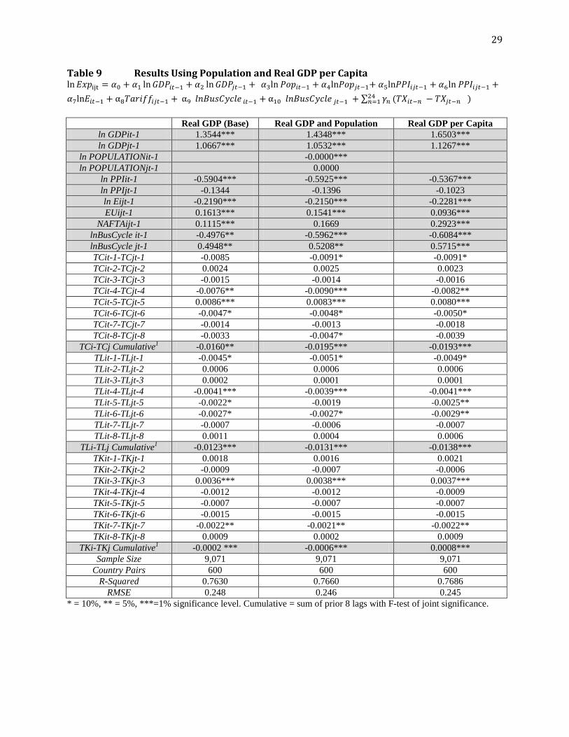
producer price indices plus the real exchange rate. In Table 9, we added

population variables, then we replaced aggregate real GDP with real GDP per

capita. Our results were largely unchanged.

V. Results

The results are reported in Table 5 for the full sample of 25 countries.

In that table and in the discussion below, the short-run refers to the impact on

exports from changes in the tax rate of the same year, which is instrumented by

the tax rate in the year immediately preceding (TXt-1). The cumulative impact

refers to the sum of the coefficients of the lagged variables from one to eight

years.

14

All three tax rates have significant effects on bilateral trade flows and

with the hypothesized signs in nearly all cases. Nearly all of the other

explanatory variables also exhibit the hypothesized values. Real GDP for the

exporting and importing country have consistently positive signs as expected.

The business cycle variables, which are measures of the relative performance of

the economy compared with the previous ten years, have negative effects in the

case of the exporting countries and positive effects on importing countries as

expected. The price level and exchange rate variables have the same signs as they

did in Bergstrand (1985; 1989) although the results in our study are stronger and

more consistent. Common membership in the EU and NAFTA was also shown to

increase exports, which is consistent with the findings of Aitken (1973), Nilsson

(2002) and Gould (1998). The exception to the expected results was the

coefficient on the WTO dummy variable which had an inconsistent sign across

different specifications.8

The significance levels of estimated coefficients of the tax rate

differentials indicate that tax changes take several years to affect trade volumes.

This fits in with our hypothesis that capital and labor supply elasticities are high

enough in the long run for taxes to be passed forward into input costs, thus

affecting the high-tax country’s exports. Likewise, in most cases the cumulative

impact of increases in the tax differential is to reduce exports, as hypothesized. In

Table 6 we examine whether our results hold up in subsamples. Subsample data

include country exports to other countries in the same subsample but exclude

exports elsewhere. Our first subsample drops countries with shorter time series to

produce a balanced panel, then splits the balanced panel into a European

subsample and a Pacific Rim subsample. Table 7 lists the countries included in

each subsample.

8 This result was also found by Rose (2004) in a gravity model specification.

15

Consumption Tax

Our hypothesis is that an increase in the difference in consumption

tax rates has a cumulative negative effect on exports since it is (indirectly) a tax

on work effort. We found this to be the case, whether we include the consumption

tax rate differential singly or in conjunction with the capital and labor income tax

rate differentials (see Table 5). The cumulative impact is negative, indicating that

countries with relatively high consumption taxes tend to export less. The effects

at a one year lag are more ambiguous. In regressions using the full data set there

is no significant impact, but in subsample regressions (Table 6) there appears to

be a significant negative short run impact especially the two subsamples

dominated by European countries. There is also fairly consistent evidence across

all regressions, including those in Tables 8 and 9, that there are significant

impacts at lags 4 and 5 but these offset each other. The only exception is the

Pacific Rim subsample. Nonetheless, the cumulative impact is still significantly

negative in all cases. Our results extend those of Keen and Syed (2006) who

found empirically that a consumption tax has no effect on exports within a three

year horizon in their sample of 27 countries. However, since we include eight

years of data, we allow time for consumption tax effects to be reflected in labor

supply decisions, which affect labor costs thus impacting export volume.

Labor Income Tax

The estimates for the cumulative impact of increases in the labor

income tax rate differential are negative whether included singly or in conjunction

with the consumption tax rate and capital income tax rate differentials (Table 5).

There appear to be significant negative impacts from increases in the labor

income tax differential at lags 4 through 6 consistently throughout Tables 5-6 and

8-9 with one exception: the European subsample. The European subsample shows

that changes in labor income tax differentials have no impact on exports at all,

either in the short run or the long run. In contrast, the subsample of Pacific Rim

16

countries shows that labor income tax increases have significantly negative

impacts. Moreover, the cumulative impact for Pacific Rim countries is large

compared to the overall sample. It is possible that this result reflects higher labor

supply elasticities in Pacific Rim countries relative to European countries.

Capital Income Tax

The capital income tax differential has a statistically significant

positive effect at lag 3 in most of the regressions; the exceptions are the Europe

and Pacific Rim subsamples. In most cases, there is a negative impact around lag

7 with the exception of the Pacific Rim subsample where it is positive. It is

interesting to note that in the Pacific Rim subsample the magnitudes of impacts of

both capital income and labor income taxes are quite a bit larger than those for the

European sample. This is in accord with the intuition that Pacific Rim economies

have more market flexibility than European economies do. Our results are also in

accord with the conclusion of Keen and Syed, that in the short run an increase in

capital income taxes creates financial outflows which are reflected in an increase

in exports. Moreover, by using a longer horizon, our results show that tax

increases eventually reduce exports. Our explanation is that, since the cost of

capital increases, prices increase and exporters’ market share is reduced.

The estimated tax rate coefficients are semi-elasticities, that is, the

percentage change in exports with respect to a one percentage point change in the

difference between the exporting and importing countries’ taxes. For instance,

the coefficient of the labor income tax ratio differential lagged one year is -0.0045

and the cumulative coefficient is -0.0123 (column 1 of Table 8). The

interpretation of these coefficients is that if a country increases its average

effective labor income tax by one percentage point while its trading partners keep

their labor income taxes constant, the result will be a decrease in exports of 0.45

percent in the current year and a cumulative decrease in exports of 1.23 percent

over eight years. To put this into perspective, using the most recent data available

17

in this dataset from 2006, if the US increased its tax rate, measured by the tax

ratio, from 23 percent of labor income to 24 percent of labor income while its

trading partners left their tax rates untouched, US exports would decrease by

0.0045 times $1.148 trillion (U.S. exports in 2006), or $5.2 billion in the year of

the tax increase. If the analysis is extended to the cumulative impact over eight

years for the same level of exports it would be 0.0123 times $1.148 trillion, or a

$14.1 billion cumulative decrease in exports.

VI. Conclusions

The cumulative impact of increased taxes on exports, regardless of

the factor on which they are levied, is significantly negative and sizable. These

impacts are particularly strong for consumption and labor income taxes. The

effects of increases in capital income tax differentials are cloaked by the financial

outflows that they induce. Tax effects on trade take several years to become

apparent, as we hypothesized. Yet our conclusions are consistent across

subsamples and specifications, countries with low taxes will tend to export more

than countries with high taxes. To summarize, our results indicate what many

have asserted: when it comes to international trade, taxes matter. There is good

reason to be concerned about the impacts of government tax policy on the

economy’s international competitiveness.

18

REFERENCES

Aitken, Norman D. "The Effect of the EEC and EFTA on European Trade: A Temporal Cross-Section Analysis." American Economic Review 63, no. 5 (Dec. 1973): 881-892.

Anwar, Sajid. “An Impure Public Input as a Determinant of Trade.” Finnish Economic Papers. (Autumn 1995): 91-95.

Anwar, Sajid. "Government Spending on Public Infrastructure, Prices, Production and International Trade." Quarterly Review of Economics and Finance 41, no. 1 (Spring 2001): 19-31.

Baxter, Marianne. "Fiscal Policy, Specialization, and Trade in the Two-Sector Model: The Return of Ricardo?" Journal of Political Economy 100, no. 4 (Aug. 1992): 713-744.

Benassy-Quere, A., L. Fontagne and A. Lahreche-Revil. “Tax Competition and Foreign Direct Investment,” Mimeo, CEPII, Paris. (2001).

Beck, Stacie, and Cagay Coskuner "Tax Effects on the Real Exchange Rate." Review of International Economics 15, no. 5 (2007): 854-868.

Bergstrand, Jeffrey H. “The Generalized Gravity Equation, Monopolistic Competition, and the Factor-Proportions Theory in International Trade.” Review of Economics and Statistics. 71, no. 1 (Feb. 1989): 143-153.

Bergstrand, Jeffrey H. “The Gravity Equation in International Trade: Some Microeconomic Foundations and Empirical Evidence.” Review of Economics and Statistics. 67, no. 3 (Aug. 1985): 474-481.

Cameron, A. Colin, Jonah B. Gelbach and Douglas L. Miller. “Robust Inference with Multi-way Clustering.” NBER Technical Working Paper No. 327. (Sept. 2006).

Carey, David, and Josette Rabesona.. "Tax Ratios on Labour and Capital Income and on Consumption." OECD Economic Studies (2002): 129-174.

Carey, David, and Harry Tchilinguirian. "Average Effective Tax Rates on Capital, Labour and Consumption." (2000).

Clarida, Richard H. and Ronald Findlay. “Government, Trade, and Comparative Advantage.” American Economic Review. (May 1992): 122-27.

http://papers.nber.org/papers/t0327

19

Egger, Peter. "Alternative Techniques for Estimation of Cross-Section Gravity Models." Review of International Economics 13, no. 5 (2005): 881-891.

Egger, Peter. "A Note on the Proper Econometric Specification of the Gravity Equation." Economics Letters 66, no. 1 (Jan. 2000): 25-31.

Egger, Peter. “Firm-Specific Forward-Looking Effective Tax Rates.” International Tax and Public Finance 16, no. 6 (December 2009): 850-70.

Egger, Peter, and Michael Pfaffermayr. "The Proper Panel Econometric Specification of the Gravity Equation: A Three-Way Model with Bilateral Interaction Effects." Empirical Economics 28, no. 3 (Jun. 2003): 571-580.

Egger, Peter, and Doina Maria Radulescu. "Labour Taxation and Foreign Direct Investment." CESifo Working Paper No. 2309 (May 2008).

Frenkel, Jacob A., Assaf Razin, and Efraim Sadka. International Taxation in an Integrated World Cambridge and London. (1991).

Gould, David M. "Has NAFTA Changed North American Trade?" Federal Reserve Bank of Dallas Economic Review (1st Quarter 1998): 12-23.

Hajkova, Dana, Giuseppi Nicoletti, Laura Vartia, and Kwang-Yeol Yoo. "Taxation and Business Environment as Drivers of Foreign Direct Investment in OECD Countries." OECD Economic Studies (2006): 7-38.

Helpman, Elhanan. "Macroeconomic Poli cy in a Model of International Trade with a Wage Restriction." International Economic Review 17.2 (Jun. 1976): 262-277.

Keen, Michael and Murtaza H. Syed. "Domestic Taxes and International Trade: Some Evidence." IMF Working Papers 06/47 (2006).

Mankiw, N. Gregory and Matthew Weinzieral "Dynamic Scoring: A_Back-of-the-Envelope Guide." Journal of Public Economics 90, nos. 8-9 (September 2006): 1415-1433.

McCallum, John. "National Borders Matter: Canada-U.S. Regional Trade Patterns." American Economic Review 85, no. 3 (June 1995): 615-623.

Mendoza, Enrique G., Gian Maria Milesi-Ferretti, and Patrick Asea. "On the Ineffectiveness of Tax Policy in Altering Long-Run Growth: Harberger's

20

Superneutrality Conjecture." Journal of Public Economics 66, no. 1 (Oct. 1997): 99-126.

Mendoza, Enrique G., Razin, Assaf, and Linda L. Tesar. "Effective Tax Rates in Macroeconomics: Cross-Country Estimates of Tax Rates on Factor Incomes and Consumption." Journal of Monetary Economics 34, no. 3 (Dec. 1994): 297-323.

Müller, Gernot J. “Understanding the Dynamic Effects of Government Spending on Foreign Trade.” Journal of International Money and Finance, no 27 (2008): 345-371.

Nichols, Austin and Mark Schaffer. “Clustered Errors in Stata.” Research Papers in Economics (Sept. 2007): http://repec.org/usug2007/crse.pdf.

Nilsson, Lars. "Trading Relations: Is the Roadmap from Lome to Cotonou Correct?" Applied Economics 34 no. 4 (Mar. 2002): 439-452.

Rauch, James E. "Business and Social Networks in International Trade." Journal of Economic Literature 39, no. 4 (Dec. 2001): 1177-1203.

Rose, Andrew K. "Do We Really Know That the WTO Increases Trade?." American Economic Review 94, no. 1 (Mar. 2004): 98-114.

Summers, Lawrence H. "Tax Policy and International Competitiveness." International Aspects of Fiscal Policies. 349-375. National Bureau of Economic Research Conference Report series (1988).

Volkerink, Bjorn and Jakob de Haan. “Tax Ratios: A Critical Survey.” OECD Tax Policy Studies No. 5 (2000).

Wooldridge, J. M. Econometric Analysis of Cross Section and Panel Data. Cambridge, Massachusetts: The MIT Press (2002).

Yoo, Kwang-Yeol. “Corporate Taxation of Foreign Direct Investment Income 1991-2001.” OECD Economics Department Working Papers, No. 365 (2003).

21

Table 1 Descriptive Statistics for Consumption Tax Rate

Observations Years Mean Minimum Median Maximum Std. Deviation

Australia 37 1970-2006 12.69 10.79 12.48 14.96 1.05 Austria 37 1970-2006 19.35 18.01 19.27 21.15 0.73 Belgium 37 1970-2006 18.97 16.23 17.57 33.48 3.80 Canada 37 1970-2006 15.18 12.87 15.30 18.39 1.44 Czech Republic 14 1993-2006 17.31 16.06 17.27 19.08 1.13 Denmark 36 1971-2006 25.50 20.50 25.36 28.00 2.03 Finland 37 1970-2006 22.38 19.55 22.58 25.38 1.41 France 37 1970-2006 17.91 16.13 18.05 20.44 1.09 Germany 37 1970-2006 14.43 13.42 14.36 15.96 0.64 Greece 37 1970-2006 13.93 11.88 13.85 16.13 1.05 Hungary 16 1991-2006 23.33 21.31 23.02 25.54 1.22 Ireland 37 1970-2006 20.21 16.22 21.08 22.88 1.85 Italy 37 1970-2006 14.30 11.30 14.93 16.81 1.68 Japan 37 1970-2006 7.02 6.13 6.72 8.30 0.65 Korea 35 1972-2006 14.46 9.33 14.57 16.93 1.73 Netherlands 37 1970-2006 17.33 16.00 17.28 19.21 0.82 New Zealand 21 1986-2006 17.96 13.85 18.12 19.79 1.13 Norway 37 1970-2006 24.73 22.26 24.49 26.93 1.31 Poland 12 1995-2006 17.09 15.51 17.09 18.58 0.93 Portugal 30 1977-2006 16.78 12.20 17.76 19.18 2.07 Spain 37 1970-2006 11.53 6.58 13.62 15.33 3.43 Sweden 37 1970-2006 19.84 16.53 20.55 21.96 1.50 Switzerland 37 1970-2006 9.15 8.02 9.03 10.47 0.68 UK 37 1970-2006 15.37 12.63 15.47 20.55 1.57 US 37 1970-2006 6.64 5.98 6.60 7.54 0.42

22

Table 2 Descriptive Statistics for Labor Income Tax Rate



23

Table 3 Descriptive Statistics on Capital Income Tax Rate



24

Table 4 Choice of Model Specification

Bilateral Fixed Effects

OLS with Country

Dummies, no Time-Invariant Bilateral Terms

OLS with Country

Dummies and Time-Invariant Bilateral Terms

Hausman-Taylor

Number of Observations 15,409 15,409 15,409 15,398 Adj. R-Squared 0.966 0.734 0.889 Root Mean Square Error 0.376 1.046 0.6771 Akaike Information

Criterion 14,986.1 45,207.3 31,809.3

Bayesian Information Criterion -20,687.6 -45,948.6 -32,581.2

Hausman FE vs. RE χ2(44) 128.31*** Hausman Overidentification

Test χ2(6) 39.928***

Wald tests: Exporter Effect 400.50*** 134.84*** 222.19*** Importer Effect 253.04*** 36.35*** 128.65*** Time Effect 52.02*** 7.54*** 15.31*** Bilateral Effect 3768.94*** Bilateral Fixed Effects 296.20***

Estimation: Constant -33.550*** -22.892*** -20.226*** -39.115*** ln GDPit-1 1.374*** 1.082*** 1.392*** 1.674*** ln GDPjt-1 1.224*** 0.916*** 0.980*** 1.318*** ln PPIit-1 -0.581*** -0.760*** -0.615*** -0.916*** ln PPIjt-1 0.100*** -0.018 0.087*** 0.085*** ln Eijt-1 -0.147*** -0.110* -0.096** 0.004 Language -1.039*** 0.896** Adjacency 0.493*** 1.472*** Distance 0.633*** 0.000*** EUijt-1 0.200*** 0.830*** 0.123*** 0.254*** WTOijt-1 -0.181** 0.105 -0.176 0.039 NAFTAijt-1 0.128** 3.333*** 0.559*** 0.080 EFTAijt-1 -0.422*** ln BusCycle it-1 0.471*** 0.494** 0.493*** 0.179** ln BusCycle jt-1 0.666*** 0.882*** 1.124*** 0.592*** * significant at 10%; ** significant at 5%; *** significant at 1%

25

Table 5 The Impact of Various Taxes on Bilateral Exports ln(𝐸𝑥𝑝𝑜𝑟𝑡𝑠ijt ) = 𝛼0 + 𝛼1 ln𝐺𝐷𝑃𝑖𝑡−1 + 𝛼2 ln𝐺𝐷𝑃𝑗𝑡−1 + 𝛼3ln

𝑃𝑃𝐼𝑖𝑡−1 + 𝛼4 ln 𝑃𝑃𝐼𝑗𝑡−1 + 𝛼5 ln 𝐸𝑖𝑗𝑡−1 +𝛼6𝑇𝑎𝑟𝑖𝑓𝑓𝑖𝑗𝑡−1 + 𝛼7 ln 𝐵𝑢𝑠𝑖𝑛𝑒𝑠𝑠 𝐶𝑦𝑐𝑙𝑒𝑖𝑡−1 + α8 ln 𝐵𝑢𝑠𝑖𝑛𝑒𝑠𝑠 𝐶𝑦𝑐𝑙𝑒𝑗𝑡−1 + ∑ 𝛾𝑛𝑚

𝑛=1 (𝑇𝑋 𝑖𝑡−𝑛

− 𝑇𝑋 𝑗𝑡−𝑛 )

All Taxes Ratios Consumption Tax Ratio

Labor Income Tax Ratio

Capital Income Tax Ratio

ln GDPit-1 1.3544*** 1.5760*** 1.3757*** 1.3745*** ln GDPjt-1 1.0667*** 1.1090*** 1.0285*** 1.0370*** ln PPIit-1 -0.5904*** -0.6573*** -0.6045*** -0.6244*** ln PPIjt-1 -0.1344 -0.1141 -0.0864 -0.0865 ln Eijt-1 -0.2190*** -0.1793*** -0.2234*** -0.1665*** EUijt-1 0.1613*** 0.1762*** 0.1691*** 0.1685*** NAFTAijt-1 0.1115*** 0.1186** 0.1123*** 0.1132*** lnBusCycle it-1 -0.4976** -0.4765** -0.4133** -0.4522** lnBusCycle jt-1 0.4948** 0.3252 0.5188** 0.4288* TCit-1-TCjt-1 -0.0085 -0.0026 TCit-2-TCjt-2 0.0024 0.0012 TCit-3-TCjt-3 -0.0015 0.0012 TCit-4-TCjt-4 -0.0076** -0.0076*** TCit-5-TCjt-5 0.0086*** 0.0079*** TCit-6-TCjt-6 -0.0047* -0.0036* TCit-7-TCjt-7 -0.0014 -0.0030 TCit-8-TCjt-8 -0.0033 0.0002 TCi-TCj Cumulative1 -0.0160** -0.00630*** TLit-1-TLjt-1 -0.0045* -0.0040 TLit-2-TLjt-2 0.0006 0.0012 TLit-3-TLjt-3 0.0002 0.0007 TLit-4-TLjt-4 -0.0041*** -0.0033** TLit-5-TLjt-5 -0.0022* -0.0020 TLit-6-TLjt-6 -0.0027* -0.0031** TLit-7-TLjt-7 -0.0007 -0.0024* TLit-8-TLjt-8 0.0011 -0.0004 TLi-TLj Cumulative1 -0.0123*** -0.0134*** TKit-1-TKjt-1 0.0018 -0.0005 TKit-2-TKjt-2 -0.0009 -0.0014 TKit-3-TKjt-3 0.0036*** 0.0033*** TKit-4-TKjt-4 -0.0012 -0.0021** TKit-5-TKjt-5 -0.0007 -0.0013 TKit-6-TKjt-6 -0.0015 -0.0016* TKit-7-TKjt-7 -0.0022** -0.0025*** TKit-8-TKjt-8 0.0009 -0.0002 TKi-TKj Cumulative1 -0.0001*** -0.00639*** Sample Size 9,071 10,720 9,364 9,195 Country Pairs 600 600 600 600 R-Squared 0.7630 0.7503 0.7566 0.7588 RMSE 0.248 0.268 0.252 0.250

* = 10%, ** = 5%, ***=1% significance level. Cumulative = sum of prior 8 lags with F-test of joint significance.

26

Table 6 Subsample Results for Tax Effects on Exports ln(𝐸𝑥𝑝𝑜𝑟𝑡𝑠ijt ) = 𝛼0 + 𝛼1 ln𝐺𝐷𝑃𝑖𝑡−1 + 𝛼2 ln𝐺𝐷𝑃𝑗𝑡−1 + 𝛼3ln

𝑃𝑃𝐼𝑖𝑡−1 + 𝛼4 ln 𝑃𝑃𝐼𝑗𝑡−1 + 𝛼5 ln 𝐸𝑖𝑗𝑡−1 +𝛼6𝑇𝑎𝑟𝑖𝑓𝑓𝑖𝑗𝑡−1 + 𝛼7 ln 𝐵𝑢𝑠𝑖𝑛𝑒𝑠𝑠 𝐶𝑦𝑐𝑙𝑒𝑖𝑡−1 + α8 ln 𝐵𝑢𝑠𝑖𝑛𝑒𝑠𝑠 𝐶𝑦𝑐𝑙𝑒𝑗𝑡−1 + ∑ 𝛾𝑛24



Full Set Balanced Set Europe Pacific Rim

ln GDPit-1 1.3544*** 1.4074*** 1.1571*** 1.8673*** ln GDPjt-1 1.0667*** 1.0585*** 0.9985*** 0.9363*** ln PPIit-1 -0.5904*** -0.6111*** -0.3957** -0.8399*** ln PPIjt-1 -0.1344 -0.1503 0.1417 -0.1003 ln Eijt-1 -0.2190*** -0.2334*** -0.1897 -0.3160** EUijt-1 0.1613*** 0.1721*** 0.1348***

NAFTAijt-1 0.1115*** 0.1098*** 0.4811*** lnBusCycle it-1 -0.4976** -0.6437*** -0.4927 -1.6615*** lnBusCycle jt-1 0.4948** 0.5048** 0.5450 1.2303*** TCit-1-TCjt-1 -0.0085 -0.0165*** -0.0155** -0.0279* TCit-2-TCjt-2 0.0024 0.0021 -0.0033 0.0100 TCit-3-TCjt-3 -0.0015 0.0017 0.0076*** -0.0267** TCit-4-TCjt-4 -0.0076** -0.0079** -0.0101** 0.0030 TCit-5-TCjt-5 0.0086*** 0.0060** 0.0014 0.0128 TCit-6-TCjt-6 -0.0047* -0.0027 0.0011 -0.0036 TCit-7-TCjt-7 -0.0014 0.0005 -0.0004 0.0124 TCit-8-TCjt-8 -0.0033 -0.0010 -0.0044 -0.0011

TCi-TCj Cumulative1 -0.0160** -0.0178** -0.0237*** -0.0211** TLit-1-TLjt-1 -0.0045* -0.0057* -0.0054* -0.0243*** TLit-2-TLjt-2 0.0006 0.0003 -0.0006 0.0139** TLit-3-TLjt-3 0.0002 -0.0025 -0.0011 -0.0056 TLit-4-TLjt-4 -0.0041*** -0.0031** -0.0002 -0.0145* TLit-5-TLjt-5 -0.0022* -0.0016 -0.0013 -0.0124* TLit-6-TLjt-6 -0.0027* -0.0030* -0.0004 -0.0169** TLit-7-TLjt-7 -0.0007 -0.0001 0.0003 -0.0298** TLit-8-TLjt-8 0.0011 0.0009 0.0015 0.0046

TLi-TLj Cumulative1 -0.0123*** -0.0150*** -0.00725 -0.0850*** TKit-1-TKjt-1 0.0018 0.0019 -0.0012 -0.0002 TKit-2-TKjt-2 -0.0009 -0.0000 -0.0012 -0.0032 TKit-3-TKjt-3 0.0036*** 0.0030** -0.0003 0.0065 TKit-4-TKjt-4 -0.0012 -0.0012 -0.0013 0.0068 TKit-5-TKjt-5 -0.0007 -0.0003 -0.0003 0.0037 TKit-6-TKjt-6 -0.0015 -0.0011 -0.0018 -0.0004 TKit-7-TKjt-7 -0.0022** -0.0036*** -0.0033** 0.0116** TKit-8-TKjt-8 0.0009 0.0020 -0.0011 0.0030

TKi-TKj Cumulative1 -0.0001*** 0.000665** -0.0106* 0.0278*** Sample Size 9,071 6,999 3,453 496

Country Pairs 600 306 156 20 R-Squared 0.7630 0.7831 0.8491 0.8947

RMSE 0.248 0.259 0.199 0.167 * = 10%, ** = 5%, ***=1% significance levels. Cumulative = sum of pior 8 lags with F-test of joint significance.

27

Table 7 Subsample Composition Subsamples Countries Included Countries Dropped

Australia, Austria, Belgium, Canada, Czech Republic, Denmark, Finland, France, Germany, Greece, Hungary, Ireland, Italy, Japan, Korea, Netherlands, New Zealand, Norway, Poland, Portugal, Spain, Sweden, Switzerland, United Kingdom, United States.

Full (25 countries)

Australia, Austria, Belgium, Canada, Finland, France, Germany, Ireland, Italy, Japan, Korea, Netherlands, Norway, Spain, Sweden, Switzerland, United Kingdom, United States

Czech Republic, Denmark, Greece, Hungary, New Zealand, Poland, Portugal.

Balanced (18 countries)

Europe (13 countries)

Austria, Belgium, Finland, France, Germany, Ireland, Italy, Netherlands, Norway, Spain, Sweden, Switzerland, United Kingdom.

Australia, Canada, Czech Republic, Denmark, Greece, Hungary, Japan, Korea, New Zealand, Poland, Portugal and U.S.

Pacific Rim (5 countries)

Australia, Canada, Japan, Korea, and U.S.

Austria, Belgium, Czech Republic, Denmark, Finland, France, Germany, Greece, Hungary, Ireland, Italy, Netherlands, New Zealand, Norway, Poland, Portugal, Spain, Sweden, Switzerland, United Kingdom.

28

Table 8 Results after Dropping Price and Exchange Rate Variables ln(𝐸𝑥𝑝𝑜𝑟𝑡𝑠ijt ) = 𝛼0 + 𝛼1 ln𝐺𝐷𝑃𝑖𝑡−1 + 𝛼2 ln𝐺𝐷𝑃𝑗𝑡−1 + 𝛼3ln

𝑃𝑃𝐼𝑖𝑡−1 + 𝛼4 ln 𝑃𝑃𝐼𝑗𝑡−1 + 𝛼5 ln 𝐸𝑖𝑗𝑡−1 +𝛼6𝑇𝑎𝑟𝑖𝑓𝑓𝑖𝑗𝑡−1 + 𝛼7 ln 𝐵𝑢𝑠𝑖𝑛𝑒𝑠𝑠 𝐶𝑦𝑐𝑙𝑒𝑖𝑡−1 + α8 ln 𝐵𝑢𝑠𝑖𝑛𝑒𝑠𝑠 𝐶𝑦𝑐𝑙𝑒𝑗𝑡−1 + ∑ 𝛾𝑛24



Base Specification No PPI

No Real Exchange Rate

No PPI or Real Exchange Rate

ln GDPit-1 1.3544*** 1.2935*** 1.3448*** 1.2745*** ln GDPjt-1 1.0667*** 1.0470*** 1.0384*** 1.0291*** ln PPIit-1 -0.5904***

-0.5747***

ln PPIjt-1 -0.1344

-0.1479 ln Eijt-1 -0.2190*** -0.1906***

EUijt-1 0.1613*** 0.1429*** 0.1606*** 0.1506*** NAFTAijt-1 0.1115*** 0.0898 0.1132*** 0.1050*

lnBusCycle it-1 -0.4976** -0.6113*** -0.5246** -0.5442** lnBusCycle jt-1 0.4948** 0.5019** 0.5618** 0.5598** TCit-1-TCjt-1 -0.0085 -0.0100* -0.0084 -0.0109** TCit-2-TCjt-2 0.0024 0.0016 0.0012 0.0020 TCit-3-TCjt-3 -0.0015 -0.0006 -0.0018 -0.0025 TCit-4-TCjt-4 -0.0076** -0.0095*** -0.0087** -0.0085** TCit-5-TCjt-5 0.0086*** 0.0078*** 0.0073*** 0.0074*** TCit-6-TCjt-6 -0.0047* -0.0041 -0.0036 -0.0039 TCit-7-TCjt-7 -0.0014 -0.0019 -0.0011 -0.0003 TCit-8-TCjt-8 -0.0033 -0.0065** -0.0019 -0.0058**

TCi-TCj Cumulative1 -0.0160** -0.0232*** -0.0170** -0.0225*** TLit-1-TLjt-1 -0.0045* -0.0054** -0.0032 -0.0055** TLit-2-TLjt-2 0.0006 0.0009 -0.0000 0.0002 TLit-3-TLjt-3 0.0002 0.0004 -0.0003 0.0002 TLit-4-TLjt-4 -0.0041*** -0.0039*** -0.0042*** -0.0027** TLit-5-TLjt-5 -0.0022* -0.0029** -0.0022* -0.0009 TLit-6-TLjt-6 -0.0027* -0.0027* -0.0011 -0.0026* TLit-7-TLjt-7 -0.0007 -0.0008 -0.0004 -0.0023* TLit-8-TLjt-8 0.0011 0.0014 0.0015 0.0012

TLi-TLj Cumulative1 -0.0123*** -0.0130*** -0.0099** -0.0124** TKit-1-TKjt-1 0.0018 0.0005 0.0015 0.0004 TKit-2-TKjt-2 -0.0009 -0.0003 -0.0003 0.0000 TKit-3-TKjt-3 0.0036*** 0.0036*** 0.0038*** 0.0034*** TKit-4-TKjt-4 -0.0012 -0.0013 -0.0012 -0.0015* TKit-5-TKjt-5 -0.0007 -0.0007 -0.0007 -0.0022** TKit-6-TKjt-6 -0.0015 -0.0019* -0.0020** -0.0016* TKit-7-TKjt-7 -0.0022** -0.0025*** -0.0019** -0.0010 TKit-8-TKjt-8 0.0009 0.0010 0.0006 0.0014

TKi-TKj Cumulative1 -0.0002*** -0.0016**** -0.0002*** -0.0011*** Sample Size 9,071 9,071 9,071 9,374

Country Pairs 600 600 600 600 R-Squared 0.7630 0.7525 0.7613 0.7493

RMSE 0.248 0.253 0.249 0.257 * = 10%, ** = 5%, ***=1% significance level. Cumulative = sum of prior 8 lags with F-test of joint significance.

29

Table 9 Results Using Population and Real GDP per Capita ln𝐸𝑥𝑝ijt = 𝛼0 + 𝛼1 ln𝐺𝐷𝑃𝑖𝑡−1 + 𝛼2 ln𝐺𝐷𝑃𝑗𝑡−1 + 𝛼3ln

𝑃𝑜𝑝𝑖𝑡−1 + 𝛼4ln𝑃𝑜𝑝𝑗𝑡−1+ 𝛼5ln𝑃𝑃𝐼𝑖𝑗𝑡−1 + 𝛼6ln 𝑃𝑃𝐼𝑖𝑗𝑡−1 +𝛼7ln𝐸𝑖𝑡−1 + α8𝑇𝑎𝑟𝑖𝑓𝑓𝑖𝑗𝑡−1 + α9 𝑙𝑛𝐵𝑢𝑠𝐶𝑦𝑐𝑙𝑒 𝑖𝑡−1

+ α10 𝑙𝑛𝐵𝑢𝑠𝐶𝑦𝑐𝑙𝑒 𝑗𝑡−1 + ∑ 𝛾𝑛24

𝑛=1 (𝑇𝑋𝑖𝑡−𝑛 − 𝑇𝑋𝑗𝑡−𝑛 )

Real GDP (Base) Real GDP and Population Real GDP per Capita ln GDPit-1 1.3544*** 1.4348*** 1.6503*** ln GDPjt-1 1.0667*** 1.0532*** 1.1267***

ln POPULATIONit-1 -0.0000*** ln POPULATIONjt-1 0.0000 ln PPIit-1 -0.5904*** -0.5925*** -0.5367*** ln PPIjt-1 -0.1344 -0.1396 -0.1023 ln Eijt-1 -0.2190*** -0.2150*** -0.2281*** EUijt-1 0.1613*** 0.1541*** 0.0936***

NAFTAijt-1 0.1115*** 0.1669 0.2923*** lnBusCycle it-1 -0.4976** -0.5962*** -0.6084*** lnBusCycle jt-1 0.4948** 0.5208** 0.5715*** TCit-1-TCjt-1 -0.0085 -0.0091* -0.0091* TCit-2-TCjt-2 0.0024 0.0025 0.0023 TCit-3-TCjt-3 -0.0015 -0.0014 -0.0016 TCit-4-TCjt-4 -0.0076** -0.0090*** -0.0082** TCit-5-TCjt-5 0.0086*** 0.0083*** 0.0080*** TCit-6-TCjt-6 -0.0047* -0.0048* -0.0050* TCit-7-TCjt-7 -0.0014 -0.0013 -0.0018 TCit-8-TCjt-8 -0.0033 -0.0047* -0.0039

TCi-TCj Cumulative1 -0.0160** -0.0195*** -0.0193*** TLit-1-TLjt-1 -0.0045* -0.0051* -0.0049* TLit-2-TLjt-2 0.0006 0.0006 0.0006 TLit-3-TLjt-3 0.0002 0.0001 0.0001 TLit-4-TLjt-4 -0.0041*** -0.0039*** -0.0041*** TLit-5-TLjt-5 -0.0022* -0.0019 -0.0025** TLit-6-TLjt-6 -0.0027* -0.0027* -0.0029** TLit-7-TLjt-7 -0.0007 -0.0006 -0.0007 TLit-8-TLjt-8 0.0011 0.0004 0.0006

TLi-TLj Cumulative1 -0.0123*** -0.0131*** -0.0138*** TKit-1-TKjt-1 0.0018 0.0016 0.0021 TKit-2-TKjt-2 -0.0009 -0.0007 -0.0006 TKit-3-TKjt-3 0.0036*** 0.0038*** 0.0037*** TKit-4-TKjt-4 -0.0012 -0.0012 -0.0009 TKit-5-TKjt-5 -0.0007 -0.0007 -0.0007 TKit-6-TKjt-6 -0.0015 -0.0015 -0.0015 TKit-7-TKjt-7 -0.0022** -0.0021** -0.0022** TKit-8-TKjt-8 0.0009 0.0002 0.0009

TKi-TKj Cumulative1 -0.0002 *** -0.0006*** 0.0008*** Sample Size 9,071 9,071 9,071

Country Pairs 600 600 600 R-Squared 0.7630 0.7660 0.7686

RMSE 0.248 0.246 0.245 * = 10%, ** = 5%, ***=1% significance level. Cumulative = sum of prior 8 lags with F-test of joint significance.

By Stacie Beck and Alexis Chaves - Lerner · By Stacie Beck and Alexis Chaves WORKING PAPER SERIES...

Documents

Transcript of By Stacie Beck and Alexis Chaves - Lerner · By Stacie Beck and Alexis Chaves WORKING PAPER SERIES...