69

THE AUDIOMAGNETOTELLURIC (AMT) METHOD AND ITS USE IN ORE PROSPECTING AND STRUCTURAL RESEARCH

by

S.-E. Hjelt, J.V. Heikka, E. Lakanen, R. Pelkonen and R. Pietilä

Hjelt, S.-E., Heikka , J.V., Lakanen, E., Pelkonen, R. & , Pietilä , R., 1990. The audiomagnetotelluric (AMT) method and its use in ore prospecting and structural research. GeoJogian tutkimuskeskus, Tutkimusraportti 95, 69· 86, 13 figs .

When the audiomagnetotelluric (AMT) method is used, several components of the Earth's natural electromagnetic field are registered simultaneously in the frequency band 1 to 10000 Hz. The primary field is produced mainly by lightning discharges and the secondary fjelds carry Information about the distribution of the electrical conductivity within the subsurface.

In Finland, the scalar variant of the AMT method has been succesfully appl ied both in ore prospecting and structural research. The present paper reviews the main properties of scalar AMT measurements and the basic principles of data processing and interpretation. Three case histories are presented .

A general structural study was made at Talvivaara in the Kainuu schlst belt. In the area of the Rautuvaara Iron mine, the scalar AMT technique was successfully used to locate gently dipping, conducting and ore-<:ritical horizons at depths ranging from a few tens of meters to about 500 meters. In a regional survey, covering about 15 km2 in the Hannukainen area, the AMT results were a relevant complement to other geophysical studies.

Some results are presented from a study made at POlvljärvi, on the Outokumpu formation, where the scalar AMT data are compared with recordings using a electrical dipolar source (so-<:alled controlled source AMT = CSAMT measurements). The CSAMT technique has superior signal·to·noise ratios, but the interpretation becomes increasingly complex.

Key words: electromagnetic induction, audiomagnetotelluric methods, sounding, inverse problem, mineral exploration, crust, case studies, Talvivaara, Hannukainen, Saramäkl, Finland

HALT. C. -3 .• IeUIa. R .B .• .l\aIaBeB. 3 .• neAIoBeB. P.H .• nB8TBAB. P .• 1990 . MarHeToTell.II.ypHqeCKHß MeTOlI Ha i3BYKOBLlX qaCTOTax (3MT) H erD npHMeHeHHe npH nOHCKax PYlIHLIX HCKonaeMLlX H B CTpYKTYPHOß reoll.OrHH. reOIl.OrH'lecKHß yeHTp tHHII.HHlIHH, PanopT HCCMlIOBaHHH 95. 69-66,111111. 13·

IIPH HCnOll.bi30BaHHH MarHeToTel\lI.ypHqeCKOrO MeTOlIa Ha i3BYKOBLlX qaCTOTax (3MT) 01IHOBpeMeHHO perH cTpHpyeTcH HeCKOl\bKO COCTaBI\HIO\llHX eCTeCTBeHHoro i31\eKTpOMarHHTHoro nOIl.H 3eMI\H B lIHanai30He qaCTOT OT 1 110 10000 rl! . IIepBHqHOe nOl\e COi3lIaeTCH npH i3TOM OOblqHO i3a CqeT MOl\HHßHLlX pai3pH,lIoB. a BTO pHqHLle nOl\H HecYT HHtOpMaYHIO 0 pacnpelIel\eHHH i31\eKTpOnpOBOlIHOCTH B nOlInOBepXHocTHOM cI\oe .

B tHHII.HHlIHH MeTOlI 3MT B CKal\HpHoß BepcHH ycneUlo npHMeHHI\CH KaK npH nOHCKax PYlILlX HCKonaeMLlX, TaK H B CTPYKTypHLlX HCCII.elIOBaHHHX. B CTaTbe npHBOlIHTCH rll.aBHLle xapaKTepHCTHKH CKal\HpHoß CbeMKH i3MT H OCHOBHLle npHHijHnLI oopaOOTKH lIaHHLlX H HHTepnpeTaijHH nOl\yqeHHLlX pei3YII.bTaTOB. B KaqeCTBe npHMepa paCCMOTpSHLI TpH ,lIeßCTBHTell.bHLlX cI\yqaH.

B Tal\BHBaapa, B npelIel\ax CI\aHl!eBoro nOHca KaßHYY, lIaHHLlß MeTOlI ynoTpeOIl.HI\CH 1III.H OO\lleCTPYKTYPHLlX HCCI\elIOBaHHß. B lI<el\ei30pY1IHOM paßOHe PaYTYBaapa CKal\HpHaH TeXHOl\OrHH i3MT OLll\a C ycnexoM npHMeHeHa 1III.H 1I.0KaIl.Hi3aYHH nOll.oronalIalO\lIHX npOBalIH\lIHX PYlIOKpHTHqeCKHX rOpHi30HTOB B lIHanai30He rll.YOHH i3all.eraHHH OT nepBLlX lIeCHTKOB MeTpoB 110 500 M. IIPH perHOHall.bHoß CbeMKe Ha TeppHTopHH OKOII.O 15 KM2 B paßOHe MeCTopoll<lIeHHH XaHHYKaßHeH lIaHHLle AMT ycneUlHo lIOnOIl.HHII.H OCTall.bHLle reotHi3HqeCKHe HCCII.elIOBaHHH.

Ha npeHMepe paßoHa IIOII.BHHpBH (noHc OYToKYMny) npelICTaBII.eHLI pesYII.bTaTLI HCCII.elIOBaHHß no cpaBHeHHIO pesYII.bTaTOB CKall.HpHOrO MeTOlIa 3MT C lIaHHLlMH, nOll.yqeHHLlMH C npHMeHeHHeM slI.eKTpHqeCKH 1IHnOIl.HpHOrO HCTOqHHKa (T .H. CbeMKa 3MT C ynpaBII.HeMLlM HCTOqHHKOM = CSAMT). TeXHOII.OrHH CSAMT HBII.HeTCH HecpaBHeHHoß no OTHOUleHHIO CHrHall.a K nOMexe, 01IHaKO HHTepnpeTaYRH pesYII.bTaTOB OKaSLlBaeTCH KpaßHe Cl\. OllCHO it

70

Description of the method

The source field and its properties

Most of the energy in the audio frequency EM spectrum (1 to 10000 Hz) is due to the energy released in lightning discharges. This energy is propagated all over the world and forms the source field for the AMT method . Because the thunderstorm activity around the world varies geographically and seasonally, the energy level changes, too. In principle the most suitable times for measurements in Finland are the summer season and the afternoon hours.

The lightning discharge is essentially a vertical electric dipole, but far away, on the measuring site , the primary fjeld can be described by plane waves. Locally the data are distorted by noise fields , mainly of man-made origin. Power-lines are especially harmful, since the measuring frequency band includes the mains frequency, 50 Hz and its harmonics. In very resistive environments, even rather high harmonics have been identified up to several kilometers from the power line.

In recent years the use of frequency sounding (FS) has increased in prospecting. Systems, in which the horizontal field components of a grounded long wire are recorded have become known in the western literature as the CSAMT (Controlled Source AMT) method (Goldstein and Strangway, 1975; Zonge et al. , 1980). The prize paid for higher signal-to-noise ratios and improved reliability of the data is increasing the complexity of interpretation.

The measurements

In complete MT measurements all four horizontal components are recorded and the most up-to-date systems make use of the additional information in the vertical magnetic field component. The components of the electric and magnetic fields E and H are linearly related

E = Z*H (1 )

The connecting factor is the impedance Z, which depends on the distribution of electrical conductivity within the Earth. It is a complex tensor, which can be mathematically rotated to obtain its extreme directions. These directions are related to those of the electrical conductivity of the subsurface, which again are controlled by geological structures, such as the strike and fractures of the bedrock.

Often AMT work is restricted to the scalar case, where only one electrical and one magnetic horizontal component are measured. Oirectional information on the impedance can then be obtained only by rotating the measuring layout at the field site and registering the field components in various directions. Scalar AMT corresponds to the classical Tikhonov-Cagniard theory (Cagniard, 1953, Tikhonov, 1950) and gives correct results for a horizontally layered medium. In Precambrian geology, scalar AMT data must normally be interpreted by 20 numerical modelling.

Equipment

In Finland, all measurements have been made with the French scalar instruments ECA 541-0 and 542-0. The systems have built-in filters for fixed frequencies. The high frequency part of AMT recordings is always checked by the VLF-R method. This gives a crucial control over the high frequency part of the AMT sounding curve, which otherwise often remains useless because of poor signal levels from around 1 to 3 kHz. The mains frequency and its first harmonics are suppressed by notch-filtering techniques.

71

Table 1. Frequencies (in Hz) of the French scalar AMT-systems 541-0 and 542-0.

541-0

542-0

Data processing

8 17 37

4,7 7,1 23

80 170

47 71

370

230

800 1700 3700

470 710 2300

The impedance tensor is usually obtained from the recorded electrical and magnetic fjeld time series using spectral methods. Instead of the impedance Z, magnetotelluric data are

usually presented as (scalar) apparent resitivities Pa and phases.

Pa = I Zij 12 /(w/J <1> = arg (Z ij)

(2)

When the tensor component ij of Z, corresponding to the electric field measured (or rotated) along the geological strike, is used, one speaks of parallel apparent resistivity Pa I 1 or E-polarization. In H-polarization results, the magnetic field component along the geological strike is used and consequently one speaks of perpendicular apparent resistivity, Pal. For a horizontally stratified Earth, Pa I I = PaL = Pa· For a homogeneous half-space, Pa equals the true resistivity of the half-space. There exist several other ways of defining the phase shift.

When AMTequipment records only two components of the EM field , only scalar apparent resistivities can be calculated. In the instruments ECA 541-0 and 542-0, this is performed electronically. At the same time, the phase information is lost.

Presentation of sounding curves

The MT results are usually presented as sounding curves , ie., Pa as a function of decreasing frequency on a log-log scale. It has become standard practice to draw AMT results directly on the H-S-nomograms already in the field . The H- and S-lines give the possibility of rapidly estimating these interpretation parameters immediately after and/or during field work. Normally, a suitable number of readings (3-5) are taken at each frequency, and their average value is drawn (together with their extremes) on the nomogram at the measuring site. When an appropriately short distance between the sounding points has been used, the presentation of all the sounding curves along a profile simultaneously gives a qualitative quick-look on the behaviour of the electrical cross-section. The 20 distortion effects (Berdichevsky and Omitriev, 1976) are easily recognized, provided sounding profiles in two perpendicular directions are used.

Electric cross sections

At the lower frequencies , the electromagnetic field penetrates deeper into the subsurface. The apparent resistivities are sometimes plotted along the profile so that the frequency decreases downwards and the Pa-values are contoured. The result is called a pseudosection, which is a rough estimate of the conductivity versus depth. If true vertical resistivity cross-sections are wanted, 20 numerical modelling is necessary for the complete

72

measuring profile. A suitable formal 1 D model is used as a starting model. For the most reliable fit, measurents in two independent directions should be used simultaneously.

1 D interpretation

Nomograms

As explained , nomograms with H- and S-lines can be used for the first quantitative interpreration even in field conditions. Since the resistivity contrasts are often large, formal 10 models give reasonable estimates for the most reliable parameters : the depth to a well-conducting layer and the layer conductance. Layer model curve fitting is also possible and may be useful when the sounding points are situated far fram each other.

Resistivity-depth transformations

Several methods have been proposed in the literature . The Niblett-Bostick transformation (Niblett and Sayn-Wittgenstein, 1960, Bostick, 1977) and its variants (Jones 1983, Goldstein and Strangway, 1975) have at present gained the greatest popularity. The transformation is very efficient as a first 10 approximation of MT data. It can be written as (Goldberg and Rotstein, 1982)

PNB(Z) = Pa(T) ( 1T / { 2q(T) } - 1) , (3)

where <I>(T) is the phase of the apparent resistivity. Alternatively the transformation can be written (Weidelt, 1972, Jones 1983) in a form suitable for calculation also from scalar data

PNB(Z) = Pa(T) { 1 + m(T) } / { 1 - m(T) }, (4)

where

m(T) = 0 {log [ Pa(T) 1/ 0 log (T)} = {T / Pa(T) } 0 [ Pa(T) I /oT

is the slope of the apparent resistivity sounding curve in log-log presentation . Two points at both ends of the sounding curve have to be sacrificed to the determination of the slope m(T) .

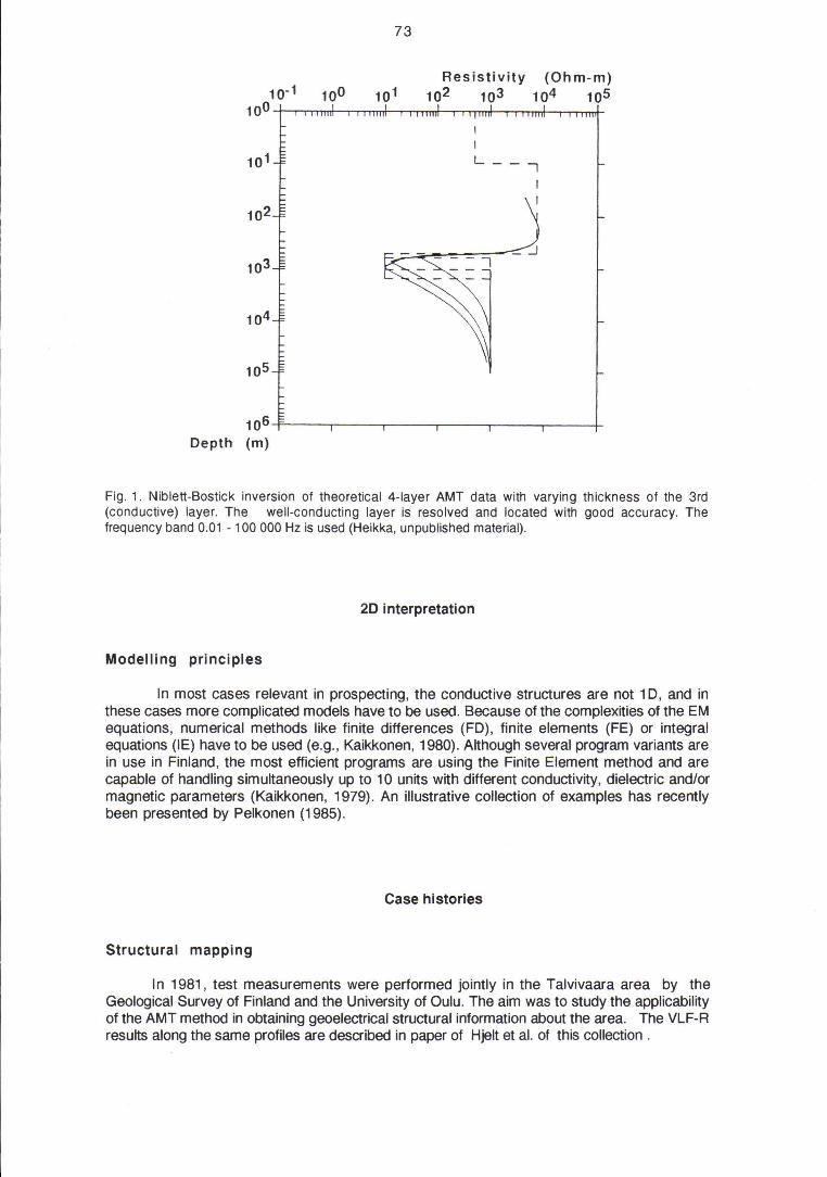
Fig. 1 shows a theoretical example of using the Niblett-Bostick transformation. The forward problem has been calculated with the recursive algorithm of Kunetz (1972). The layers are shown by dashed lines. The transformation gives realistic depths and conductivities for conducting layers. The transformation works less weil for resistive layers.

Curve fitting

For selected soundings, where a closer model is required , a layer model can be fitted to the data by standard least-squares inversion (optimization) techniques. The method consists of fitting the logarithm of apparent resistivity by the so called hyberparabolic method (Lakanen, 1975), where 2-4 model parameters (Iayer resistivities and thicknesses) are optimized simultanously. A layer model fit (Peikonen et al. , 1979) seldom significantly impraves the model obtained from, H-S-line estimation, pravided proper distortion corrections have been applied.

- - - --- ------------------------------------------

73

Resistivity (Ohm-m) 10-1 100 101 102 103 104 105

10°;-Tr~r.~~-.nmmr"nm~rn~~on~ I I L __ -,

I

106~----.----.----_.----._--_,r_--_+ Depth (m)

Fig. 1. Niblett-Bostick inversion of theoretical 4-layer AMT data with varying th ickness of the 3rd (conductive) layer. The well-conducting layer is resolved and located with good accuracy. The frequency band 0.01 - 100 000 Hz is used (Heikka, unpublished material).

20 interpretation

Modelling principles

In most cases relevant in prospecting, the conductive structures are not 1 D, and in these cases more complicated models have to be used. Because of the complexities of the EM equations, numerical methods like finite differences (FD), finite elements (FE) or integral equations (IE) have to be used (e.g. , Kaikkonen, 1980). Although several program variants are in use in Finland, the most efficient programs are using the Finite Element method and are capable of handling simultaneously up to 10 units with different conductivity, dielectric and/or magnetic parameters (Kaikkonen, 1979). An illustrative collection of examples has recently been presented by Pelkonen (1985) .

Case histories

Structural mapping

In 1981 , test measurements were performed jointly in the Talvivaara area by the Geological Survey of Finland and the University of Oulu. The aim was to study the applicability of the AMT method in obtaining geoelectrical structural information about the area. The VLF-R results along the same profiles are described in paper of Hjelt et al. of this collection .

A)

C)

i o

Kajaani .. Sotkamo

200km I I

1KM

74

B)

G o -

Presvecokarelidic complex

Quartzite

Phyllite , black schist

o ~

Granite

Mica schist

Garnet-hornblende schist

AMT-sounding VLF-R-profile

• Ni-Cu - Zn - mineralization

• Block schist

~ Mica schist

D Quartziti!'

~ 5I!'rpentinite

~----~~~~~~~r-----------+---~------+-----------T-----------,---~m95

553 556

Fig. 2. Location (A) and geology (8) & (C) (Heino and Havola, 1980) of the survey area of Talvivaara in the southern part of the Kainuu schist belt.

75

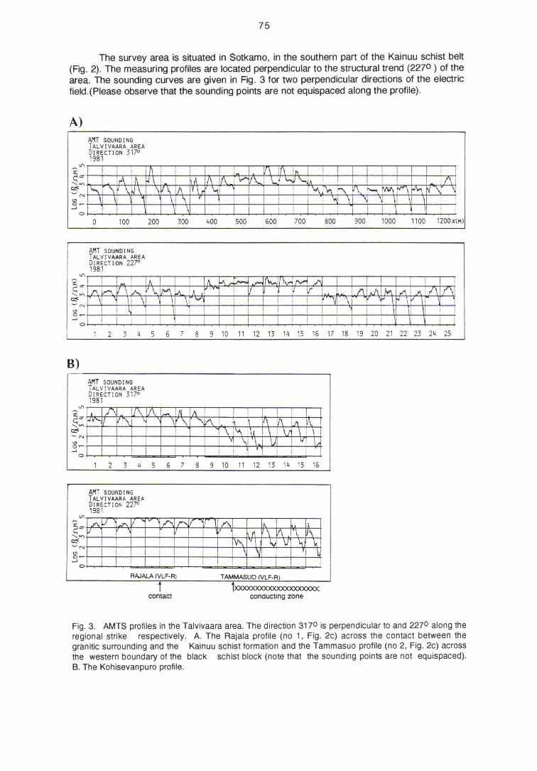
The survey area is situated in Sotkamo, in the southern part of the Kainuu schist belt (Fig. 2) . The measuring profiles are located perpendicular to the structural trend (2270 ) of the area. The sounding curves are given in Fig. 3 for two perpendicular directions of the electric field.(Please observe that the sounding points are not equispaced along the profile).

A) AMT SOUND ING TALVIVAAR A ARE A DI RECTl ON 3170

1981

~~RmiNml$fftj~@

o

B)

o 100 200 300 400 500 600 700 800 900 1000 1100 1200 X(M)

AMT SOUND ING TALVIVAARA AREA DI RE CTl ON 22JO 1981

I I 1 I" I 1'\ Ir--. V \ 0.. V \..IM l\ ~ ~ \1 \1 ~ \ I ! ~ 1 i ,

I

I I I ! I

l\. 1..\ ;...-. ..,.... If\..., Ih i ,

\ 'V I I I I I I

i I :

"V"I~ .'" 1 1 i I I

V Ir , ! Y\ 1 ./\ M "" )\ 1\ 1(\ I ! " '\ I- r \ r-; \ \ \f I 1 1 I \ \ I I I i i I I i i

2 3 4 5 6 7 8 9 10 11 12 13 14 15 16 17 18 19 20 21 22 23 24 25

AMT SOUND ING TALV l vAARA AREA DIR ECTlON 31 70

1981

2 3 4 5 6 7 8 9 10 11 12 13 14 15 16

AMT SOUNDING TALVIVAARA AR EA DI RE CTl ON 2270 1981

I

!~br e rrrrrnmtfl RAJALA (VLF·R)

contact

Fig. 3. AMTS profi les in the Talvivaara area. The direction 3170 is perpendicu lar to and 2270 along the regional strike respectively. A. The Rajala profile (no 1, Fig. 2c) ac ross the contact between the granitic surrounding and the Kainuu schist formation and the Tammasuo profile (no 2, Fig. 2c) across the western boundary of the black sch ist block (note that the sounding points are not equispaced). B. The Kohisevanpuro profile.

76

The contact between the resistive (mica schists) and conductive (black schists) blocks of the area is sharp when the electric field is measured in the 2270 direction. Because of the approximate two-dimensionality of the structure, this can be considered as the E-polarization direction. Above the conductive schist belt formation , the low frequency parts of all the sounding curves have a decreasing slope. Also the general level of apparent resistivity is lower than above the resistive areas.

A)

LEG END ,

------ f AULT OA FRACTURE UNE

e TRACE OF AX IAL PL ANE OF ANTIClINE

- - x- - TRACE OF AXIAL Pl AN E OF SYNClINE

--.... FQLIATION DIP, 45

-+- VERTICAl FOLIATION

UNEATION

,.- MINOR FQLD AXIS

AIA8()RNE Mo\GNETIC "'AP 8Y

AAUIARUUKtU CI'( t<J 76

1'fI01OM .... GNfTOfIIff(1t AfSO\UflON , .. ,

4VUI AOE AUUUOI XI ..

l " AV(IISl Sf.H.1I"'''0't lOQ ...

' HE COHTO\JR V"LUES Allt:

HUNOAfOS ~ "T It(DUCEO SV so,,, 'Hf ' loI 'fItVAU Of co.nOUII!i . Rt: ,

100 .. ' .('WEf" J6OO . 4000 .. 1

TECTONIC AND MAGNETIC MAP OF THE

RAUTUVAARA AREA

by AIMO HILTUNEN 1981

't 1'1

o I> "" I

..

. .

•.• jd~~' :< ~ . .

. . / . / : : : 1: . . .... X 7496.80

.•. , •. . KIVIVUOprO .·

. t: I . . \ ,. \. . I :\ . ... / :

.. .. : ,~....;./" LEGEND :

MONZONITE

DIORITE

l

X 7496.20

SKARN ORE QUARTZ _ ~~~~~~~A FELDSPAR SCHI~ AMPHIBOLITE

QUARTZITE ~~1~"'r~~, ---1 OUARTZITE COMP\.EX

HORIZONTAL ""OJECTION

Cf' OllE BOOY

77

GEOLOGICAL MAP

HANNUKAINEN A . HILTUNEN

o SOOm

Fig. 4. The tectonic and magnetic map of the Rautuvaara area (A) and the Hannukainen deposits (8). (Hiltunen, 1981).

Mapping of conducting horizons

The first application of the AMT method to mineral prospecting in Finland was made in 1976 near the Rautuvaara iron mine of Rautaruukki Oy (Peikonen et al. , 1979). The sounding points were located mainly along the profile x= 96.80, which traverses the gently dipping, conductive (1 to 100m) skarn iron ore lenses of the Hannukainen area. This survey, carried out as a co-operative study by Rautaruukki Oy and the Department of Geophysics, University of Oulu, with the French ECA 541 -0 system, revealed deeper continuations to the known ore lenses along the dip. Hole R-162 was drilled in response to the AMT results . A conductive magnetic layer was found at a depth of 417 m, in fairly good agreement with the AMT interpretation .

Encouraged by the first experimental AMT survey and the favourable geological structure of the area, more extensive AMT surveys have been conducted later in several stages. In 1981 an extensive, systematic AMT survey was carried out in order to map the deep ore reserves of the Hannukainen area. Within the area (Fig. 4) ,15 km2 of scalar AMT data were

78

obtained using the new ECA 542-0 system. Altogether 950 sites were sounded in a grid of 200 m by 100 m (sometimes 50 m) .

In a region where the depth of the conducting layer was known, the azimuthai dependence of the apparent resistivity was studied. Within reasonably small e margins of error, the depth of the conductive layer was obtained trom the sounding curves for most measuring directions. The S-values (conductivity x thickness) are different only if determined trom EW directed scalar soundings. The direction of the E-polarization of the AMT field was assumed to be in major parts of the area parallel to the geological strike. Thus the systematic AMT survey was performed measuring the E-field along this strike.

RnllrnRIIIJl<I<I OY Exp l orat ion

KOI nr~ I , I ImJNUI<R 1 NEN

npr'nREtn r~[SlSTIVITY RIIOa [Ohmm]

PROF I LE l'lnl"

1 : 20 Om:l

FREQ . =2 3 Hz

1 DECnllE IN L. OG(RI IOa ) = El . 5 cm

BnSE L.EVEL 3

o lkm ''---'--'---'---'---''

Fig. 5. Apparent resistivity profile map of the Hannukainen AMTS area for the frequency of 23 Hz.

79

The weil known energy minimum ot the source tield around 1 to 3 kHz was clearly noted during the whole survey. Thus the resistivities tor this trequency band had to be omitted trom the interpretation in most cases. These data were replaced by the apparent resistivity value trom VLF-R-measurements at 16.4 kHz. The interpretation included the three main steps , data processing (presentation of sounding curves and removal of unreliable data points) , 10 inversion and qualitative estimation of 20 and 3D effects . The sounding curves were plotted on the HP 98458 desktop computer of Rautaruukki Oy Exploration. From the data base created, a great variety of graphical representations could be easily obtained, individal sounding curves, profile and contour maps , pseudosections or residual profiles. A 10 interactive curve fitting system was included in the data processing.

Xo

RAUTARUUKK I OY Exploration

KOLARIo HANNUKAINEN AMT - CONTOUR MAP

APPARENT RESISTIVITY RHOa (Ohmm)

1 : 20 000 o 1km FREQ . =23 Hz I 0 0 0 o I

x 96.80

96 .00

95.00 ';;;;------'""""'"-',.AoIO"--....-=~~..L-.L-.L...<::I>.L:::...-L--Ll.I.\L.l4IL _____ ."J .. 00

- Im [',:] G""'"J

<1 .6 1.6 - 1.8 1.8 - 2 .0 2 .0-2 .8

~ ~ >2 .8

Fig. 6. Apparent resistivity contour map of the Hannukainen AMTS area for the frequency of 23 Hz.

A)

B)

RAUTRRUUKK I OY Ex p l orat ion KOLARI ,HANNUKAI NEN ?SEUDOSECTI ON APPARENT RESIST IV I TY RHO. ,Onmm l t: 2 0 000

" .. " .. " . ... ". ' 3.

73

.. '3

" 7. 3

.. , CO CO CO

:l I

PRO, .: . -96000 t OECACE IN LOGeRHOa ) • 0.5 c m BASE c.EVEL 3

! :l: I

>- >-

~AUTARUUKK I OY ~x p ioratlon

~OLARI, rlANNUKAINEN

~E5IOUAL " AP

1l! ~ I >-

nPPARE NT ~ES I S TIVITY ~HO a ( OhMm J

t : 20 al!l! .'RO' .: . - 'l 601!0 ! JECAOE :N LOG<RHO a ) • ~.5 c m

80

o 1km , ,

.. .. .. .. CO .. .. : .. ::: .. I I ~ >- ,., I ,.,

o 1km , ,--- - - - ----_._ - -------_._-------_._ - ----,

. • ~~-"nu· t~·uq,,-,.u"u"""·""· "-'t"-")(U""-,,,,-,=u,,,,-"-,,w.'''''·t~'''''l~U:[IP??~<'"'I'''''' ____ [

". t--_~ _ __"__",........,'"'_"_~T.LU·U :t.AA. tLfllrr n D (fJ r~LT[]Tl~­

... t---~~~·ll.lJ:ul.Wn....A [J.~ra:c.1TLl1~­

". t--_---I.-'-'-''--'-~,cLLUf(nU-L1LLLI.LtJ:L..d:.1 [ t) , t, 6" ,. ~ca:mr:-rrrr[r:~--

" . t-___ Lt~L..c=·-"t~,..J.(Ltfurl:u.Li:llIL..dWÜLU:_________..~nrn "n~ T7~'~' ~J ----1 ~P-J::.rro::rry

,iTrT! rrt [ ,I! ~ c1tfllrcD- ~rQl[[l[ fITTTT- r;.'·'-'--r· ·,L---_ _ -j '-1.. I , l..Y

13 r · -

.. r- _ r r'" .([ t rt,a t tr(~ , ([l::i1I:tA::..~[l.J.QlnmTI~[r::Ll---" , (' .[\

2l I-___ Lr'-'~'-T·L<=~."-LL-crl [['rr t rt CI]:, <1 tx D [<0' , ~lil4(,jUDTI::L .1 -\

" t--_ _ L.rr~r'_'·r~"__'dJ1LU)It.u'· '.ll.U. rd'l lt...dt.:JlJ:cl:J:~nllP:::p.~T1.L-------i

t 1 ( ()., rdtd (f': crten C((Yt h ' , _ .A~ _ _ -j 7.3

... • 'lJ:q,n;I;l,rp:~~~

<>!li A'f r..Ll,. <.fi. 1..C1....tLl'd,. "",Y'{JJAI~~/L-I'

I----.-----r---------.-,-----------~-----~---- .. - -N co

~ I ,.,

III ~ I >.

'" CO co CO CO . >-

Fig. 7. Apparent resistivity pseudosections (A) and residual profiles (8) of the Hannukainen AMTS area.

81

A reasonable accuracy was obtained with1 D interpretations using the simple H-S-line technique (Berdichevsky, 1968), since the geology of the area was clearly layered and the resistivity contrast between the conductor and the surrounding rock was great (>300). Some problems of equivalence were studied more in detail using the 1 D curve fitting method (Peikonen et al. , 1979) . Figures 5 and 6 give a curve presentation for the qualitative interpretation stage. From profile (Fig. 5) and contoured (Fig. 6) Pa maps, the initial estimate of the geoelectrical cross-section can be obtained approximately at the skin depth of the frequency in question . The pseudosection (Fig . 7A) gives simultaneously lateral and frequency dependent variations of apparent resistivity. In the residual technique (Koziar, 1976), apparent resistivity profiles are constructed by normalizing the resistivity values with the regional average at each frequency. The most resistive and most conductive parts of the survey are easily separated (Rg. 7B).

500

1000

1500

2000 depÖ'l

[m ]

KUEIIIoIWIA OREBOOY

RAUT ARUUKKI OY Exploration

HANNUKAINEN 1981

AMT - interpretation by layered model

_ conductor 4 S-value

- station "'~ drtllhole

~ 0 .. body

Fig. 8. 1 D interpretation of the Hannukainen AMTS data along profile X = 96.80. Drill holes DH 182, DH 197, and DH 162 intersected conducting and magnetic material at depths corresponding to the conducting layers of the 1 D model.

In the 1 D interpretation result (Fig. 8) , the eastern part of the conductor is associated with the known ore body. The plotted 1 D conductor depths give the impression of a continuous, gently dipping structure. At the extreme sounding sites in the western part of the profile, the depth of the conductor increases rapidly. This is a typical behaviour of 1 D inversion close to the edge of a 2D (or 3D) structure. By measuring at such locations, the azimuthai properties of the apparent resistivity, 2D effects are easily recognized also trom scalar AMT data (for tensor MT data, such parameters as the skew and tipper give corresponding information).

The AMT method played a very important role when the ore bodies of the Hannukainen area were mapped with geophysical methods (Hattula, 1978). The AMT data gave valuable information about both the horizontal and the vertical location of conducting structures related to the ore formations in the area.

6 403333F

82

Use of controlled sources

In 1980, the Outokumpu Co did CSAMT field work using arented Geotronics Co. EMT-5000 (transmitter) and EMR-1 (receiver) system. The apparent resistivities are calculated separately at 16 frequencies from 1 to 9600 Hz. The test aimed at a comparison of the CSAMT results with earlier natural field scalar AMT results.

Ou lu

OUTOKUMPU REGION r'fiil ~town

LEPPÄVIRTA REGION [] o

Enonkosk i

o Vammala

Fig. 9. Map marking the location of the Outokumpu formation.

Tests were made during a two month period in the Polvijärvi area , northeast of the town Outokumpu (Fig. 9) . The Outokumpu formation includes a horizon with copper-ore potentiality. The horizon extends to the north and includes a small mineralization at Saramäki. The geology of the Outokumpu formation has been described in detail by Koistinen (1981), and the geophysical work done in the area has been summarized by Ketola (1979) . The AMT measurements in the area have been described by Lakanen (1986).

In the first CSAMT test, the signal levels and the distortions of the Tikhonov-Cagniard conditions were established. The transmitted power was about 3 kW, the source dipole length (the length of the current cable)100 m and the resistivity of the environment on the average 5000 Dm. A comparison between the CSAMT and AMT soundings is shown in Fig. 10. A fracture zone, located about 1.6 km from the transmitter, caused an anomaly, which made a comparison difficult. The increasing distortion of apparent resistivity from the Tikhonov-Cagniard-condition , when approaching the transmitter site , is evident. The resistivities at low frequencies differ by a factor of 4 and higher frequencies by a factor of less than 2, approximately as expected from theoretical considerations (e.g., Kaufmann and Keller, 1983). The low level of resistivity is attributed to a conductive horizon at depth.

10'

10

POLVIJÄRVI AREA

TRANSMITTER SITE No . 1 5HI' . E-POl -<>-­No. 3 SH~ . H- POL --0--

NATURAL SOURCE 8HI , E-POl --0-

8H' , H-POl

tRANSMITtER SITE NG . !

1 ~~~~--~---L--~L----L-4~~ Y-56 .00 57 58 59 60 61 -= 62

A SURVEY lINE A B

83

10

TRANSMITTER SITE No 1 : 32Hz . E -POL ---0--­No 3 ' 32Hz .H-POl -~-

NATURAL SOURCE 37 Hz . E - POL --0--37HI.H-POL •

Y-56 .00 57 58 59

B

TRANSMITTER SIT[ Ne . 1

6 0 61 ':' 62

Fig. 10. Comparison of CSAMT and AMT apparent resistivity profiles in the Polvijärvi area of the Outokumpu formation. A. Lowest AMT frequencies (5-8 Hz), B. medium AMT frequencies (32-37 Hz).

At the lowest frequencies (5 Hz) the magnetic field component became too weak to be measured when the distance trom the transmitter approached 3 km. The apparent resistivity of the CSAMT was still two orders of magnitude higher than for the natural source AMT (8 Hz). At 32 Hz a useful signal was still obtained 4 km away trom the source. The measured mode was in principle equivalent to E-polarization.

When a long transmitter cable (3000 m) was used in the H-polarization mode, the level of the magnetic field signal was accordingly strongly enhanced. At 5 Hz (compared with 8 Hz fo AMT) the apparent resistivity values differed by a factor of 5 to 10, whereas the same values were obtained at 32 Hz. The result supports the 3 times skin-depth condition given by, among others, Goldstein and Strangway (1975).

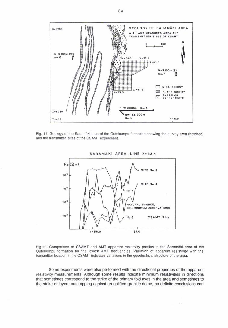
With its complex but well-studied geology, the Saramäki area is interesting target for geoelectrical studies. There is an abundance of long, good conductors, which crop out and dip gently (200 to 300 ) towards the east. One of the profiles of Fig. 11 was surveyed using four different transmitter sites (Nos. 4-7 in the Figure). All the transmitters are located at a distance of 3 km from the measuring site. The results on the lowest frequencies (5 and 8 Hz, respectively, Fig. 12) along profile X = 82.4 differ markedly depending on the location of the transmitter.

Transmitter location 4 is closest to the H-polarization mode situation, whereas the others can be more or less approximated as E-polarization modes. The lowest resistivities are naturally obtained for transmitter position 6, wh ich is located on the footwall side of the bed with several conducting layers. When the results are interpreted by 10 modelling, the most consistent results are obtained for the AMT data. The depth to the conducting horizon connected to the drilled ore formation is weil resolved. The orebody is very highly conductive, with a conductivity of more than 1000 S/m. (The black schists are accounting for only 10 to 100 S/m and the rest of the formation trom 1 to 0.01 S/m.). The best CSAMT interpretation using this technique is obtained for transmitter position 6. A 20 modelling test yielded a much broader anomaly than the measured one when a single conductor was located at the depth of the drilled ore body (Fig. 13).

84

X=6985 GEOLOGY OF SARAMÄKI AREA

WITH AMT MEASURED AREA AND TRANSMITTER SITES OF CSAMT

0 lkm N

I I

~ N-S 100m(W) No . 6 I

X - S3.0

N-Sl00m(E) No . 7 I

0 MICA SCHIST

~ BlACK SCHIST

r;::] SKARN OR SERPENrJNITE

E-W 2000m No . 4 X=6980

'NW-SE 300m •

Y·452 No . 5 Y· 459

Fig. 11. Geology of the Saramäki area of the Outokumpu formation showing the survey area (hatehed) and the transmitter sites of the CSAMT experiment.

SARAMÄKI AREA . lINE X=82.4

10~

f'"' -0.... -0- _--'\

I \ , \ , \ , \ I

\ I

J

SITE No . 5

SirE NO . 4

No.6 CSAMT . 5 Hz

Y-56 .0 57.0

Fig.12. Comparison of CSAMT and AMT apparent resistivity profiles in the Saramäki area of the Outokumpu formation for the lowest AMT frequeneies . Variation of apparent resistivity with the transmitter loeation in the CSAMT indieates variations in the geoeleetrieal strueture of the area.

Some experiments were also performed with the directional properties of the apparent resistivity measurements. Although some results indicate minimum resistivities in directions that sometimes correspond to the strike of the primary fold axes in the area and sometimes to the strike of layers outcropping against an uplifted granitic dome, no definite conclusions can

be made based on these limited tests.

'00 ...

400 ...

'00_

'00. OlPfM

y, S6 0

50 %

50 z

'0 z

A· CSAMT , SOURCE SirE NO. 5 (infig . • '

.00. 1

"'560

~. z"

'00_

IOD ... 128 % 1\2 I

C CSAMT. SOURCE StrE NO. 7

y. 51 0

o MIC. CNf:ISS

r::::l .l ACK SCHISf

o 'Mo A"'''' . O'U

o 20 0 ... ..............

y. 570

85

5X Y' 570

'00 ... 13X

tao ...

100 ...

o 200", '=='--'

B CSAMT . SOURCE 5tH NO. 8

" ·S60 "'570

' 00 ...

0 .8_ 0 . 8 z ,

.00_

.00_ X"

o 200m '=='--'

Fig. 13. 10 inversion results of three CSAMT soundings with different transmitter sites (A.- C.) and the inversion of AMTS data (0 .). The geological cross section is indicated in A and the existing boreholes in all the sections interpreted.

It is evident that more elaborate interpretation procedures are needed for CSAMT data, although performance of the measurements in the field are easier and quicker to perform. Higher power could in principle be used to increase the signal-to-noise ratio at greater distances, but then safety problems and disturbances from , e.g., general telephone communication will arise. The use of loop transmitters seems to require, according to theoretical estimations, still higher power.

References

Berdichevsky, M.N. , 1968. 3l1.eKTpHCeQKag paSBe.llKa MeTO.llOM MarHHT OTell.lI.l>IpHCeQK Or O

npo~HlI.HpOBaHHg . Nedra, Moscow, 255 pp. Berdichevsky, M.N. & Omitriev, V.I. , 1976. Basic principles of interpretation of

magnetotelluric sound ing curves. In A. Adam (ed .): Geoelectric and geothermal studies . Akademiai Kiad6, Budapest, 165-221.

Bostick, F.X ., 1977. A simple and almost exact method of MT analys is. Workshop on Electrical Methods in Geothermal Exploration, U.S. Geol. Survey, Contract No 14080001 - 8 - 359.

Cagniard, l., 1953. Basic theory of the magnetotelluric method of geophysical prospecting. GeophysicS18, 605-635.

Goldberg, S. & Rotstein, Y. , 1982. A simple form of magnetotelluric data using the Bostick

86

transform . Geoph. Prospecting 30, 211 -216. Goldstein , M.A. & Strangway, D.W. , 1975. Audiofrequency magnetotellurics with grounded

electric dipole source. Geophysics 40, 669-683. Hattula, A. , 1978. Charged potential method (mise-a-Ia- masse) in Hannukainen and Sokli area of

northern Finland. Geoexploration 16, 311 (abstract only). Heino, T., & Havola, M., 1980. Geology. of the Jormasjärvi-Talvivaara area (in Finnish). Report

M 19/3344/-80/3/10, Koskee 3433, Sotkamo, Talvivaara. Geological Survey of Finland. Hiltunen, A. , 1981 . The precambrian geology and skarn iron ores of the Rautuvaara area, northern

Finland. Bull . Geol. Survey of Finland 318,133 pp. Jones, A.G ., 1983. On the equivalence of the "Niblett" and "Bostick" transformations in the

magneto-telluric method. J. Geophys. 53, 72-73. Kaikkonen , P., 1979. Numerical VLF modeling. Geophys. Prospecting 27, 815-834. Kaikkonen, P., 1980a. Numerical VLF, VLF-R and AMT profiles over some complicated models .

Acta Univ. Oul. A 91 , Phys. 16, 34 pp. Kaufmann , A .. A .. & Keller , G.V. , 1983. Frequency and transient soundings . Elsevier,

Amsterdam-Oxford- New York, 685 pp. Ketola, M. , 1979. On the application of geophysics in the indirect exploration for copper suplhide

ores in Finland. In P.J. Hood (ed): Geophysics and geochemistry in the search for metallic ores. Econ. geology report 31, Geol. Survey of Canada, 665-684.

Koistinen, T .J., 1981. Structural eVOlution of an early Proterozoic strata-bound Cu-Co-Zn deposit, Outokumpu, Finland. Trans. Royal Soc. Edinburgh, Earth Sciences 72, 115-158.

Koziar, A., 1976. Applications of audiofrequency magnetotellurics to permafrost, crustal sounding and mineral exploration . Ph.D. Thesis, Univ. Toronto, Toronto, Ont. Canada.

Kunetz, G. , 1972. Processing and interpretation of magnetotelluric soundings . Geophysics 37 , 1005-1021 .

Lakanen, E. , 1975. An overall computer graphics software for geophysical profile interpretation. Geop. Prosp. 23, 606 (abstract only).

Lakanen, E., 1986. Scalar-AMT applied to base metal exploration in Finland. Geophysics 51 , 1628-1646.

Niblett, E.R. & Sayn-Wittgenstein, C., 1960. Variation of the electrical conductivity with depth by the magnetotelluric method. Geophysics 25, 998-1008.

Pelkonen, R., 1985. On numerical AMT profiles and sounding curves over some two-dimensional structures. Department of Geophysics, University of Oulu , Report No. 11., 57 pp.

Pelkonen, R. , Hjelt , S.-E ., Kaikkonen, P. , Pernu, T. & Ruotsalainen, A. , 1979. On the applicability of the audiomagnetotelluric (AMT) method for .ore prospecting in Finland . Contribution, Dept. of Geophysics, Univ. of Oulu, No 94, 25 pp.

Tikhonov, A.N. , 1950. Onpe.ztel\eHHe Sl\ eKTpHCeqKHX xapaKT epHcTHK rl\hlOOKHX ql\OeB

SeMH O)K KOpH . ZlOKl\ . A K a .zt . H ahlK CCC P:73, 295-297 . Weidelt , P., 1972. The inverse problem of geomagnetic induction. Zs. f. Geophysik, 38 , 257-289. Zonge, K.L. , Emer, D.F. & Ostrander, A .G. , 1980. Controlled source aud io-frequency

magnetotelluric measurements. Geophysics 46: 460 (abstract only).