by Ruslan Salakhutdinov A thesis submitted in conformity with the ...
84
LEARNING DEEP GENERATIVE MODELS by Ruslan Salakhutdinov A thesis submitted in conformity with the requirements for the degree of Doctor of Philosophy Graduate Department of Computer Science University of Toronto Copyright c 2009 by Ruslan Salakhutdinov
Transcript of by Ruslan Salakhutdinov A thesis submitted in conformity with the ...

LEARNING DEEP GENERATIVE MODELS
by
Ruslan Salakhutdinov
A thesis submitted in conformity with the requirementsfor the degree of Doctor of Philosophy
Graduate Department of Computer ScienceUniversity of Toronto
Copyright c© 2009 by Ruslan Salakhutdinov

Abstract
Learning Deep Generative Models
Ruslan SalakhutdinovDoctor of Philosophy
Graduate Department of Computer ScienceUniversity of Toronto
2009
Building intelligent systems that are capable of extracting high-level representations from high-dimensional
sensory data lies at the core of solving many AI related tasks, including object recognition, speech
perception, and language understanding. Theoretical and biological arguments strongly suggest that
building such systems requires models with deep architectures that involve many layers of nonlinear
processing.
The aim of the thesis is to demonstrate that deep generative models that contain many layers of latent
variables and millions of parameters can be learned efficiently, and that the learned high-level feature
representations can be successfully applied in a wide spectrum of application domains, including visual
object recognition, information retrieval, and classification and regression tasks. In addition, similar
methods can be used for nonlinear dimensionality reduction.
The first part of the thesis focuses on analysis and applications of probabilistic generative models
called Deep Belief Networks. We show that these deep hierarchical models can learn useful feature
representations from a large supply of unlabeled sensory inputs. The learned high-level representations
capture a lot of structure in the input data, which is useful for subsequent problem-specific tasks, such
as classification, regression or information retrieval, even though these tasks are unknown when the
generative model is being trained.
In the second part of the thesis, we introduce a new learning algorithm for a different type of hier-
archical probabilistic model, which we call a Deep Boltzmann Machine. Like Deep Belief Networks,
Deep Boltzmann Machines have the potential of learning internal representations that become increas-
ingly complex at higher layers, which is a promising way of solving object and speech recognition
problems. Unlike Deep Belief Networks and many existing models with deep architectures, the approx-
imate inference procedure, in addition to a fast bottom-up pass, can incorporate top-down feedback.
This allows Deep Boltzmann Machines to better propagate uncertainty about ambiguous inputs.
ii

Acknowledgements
First and foremost, I would like to thank my advisor GeoffreyHinton for being an incredible advisor,an amazing teacher, and providing me with a warm and outstanding intellectual environment at theUniversity of Toronto. I would also like to thank Sam Roweis,my second advisor, and my committeemembers, Radford Neal and Rich Zemel, for their valuable feedback, support, and guidance.
Many thanks goes to the members of the Toronto Machine Learning group: Andriy Mnih, IainMurray, Vinod Nair, Ilya Sutskever, and Tijmen Tieleman formany interesting and inspiring discussions.
I also thank my parents and my family for their continuing support. Finally, a special thank yougoes to my wife Olga for being supportive and putting up with me.
iii

Contents
1 Introduction 11.1 Contributions of This Thesis . . . . . . . . . . . . . . . . . . . . . . .. . . . . . . . 21.2 Summary of Remaining Chapters . . . . . . . . . . . . . . . . . . . . . .. . . . . . . 3
2 Deep Belief Networks 52.1 Restricted Boltzmann Machines . . . . . . . . . . . . . . . . . . . . .. . . . . . . . 52.2 A Greedy Learning Algorithm for Deep Belief Networks . . .. . . . . . . . . . . . . 72.3 Generalizing RBM’s to Modeling Real-valued and Count Data . . . . . . . . . . . . . 11
3 Learning Feature Hierarchies with Deep Belief Networks 153.1 Learning Features for Discrimination and Regression . .. . . . . . . . . . . . . . . . 15
3.1.1 Gaussian Processes for Regression and Binary Classification . . . . . . . . . . 163.1.2 Learning the Covariance Function for a Gaussian Process . . . . . . . . . . . . 173.1.3 Experimental results . . . . . . . . . . . . . . . . . . . . . . . . . . .. . . . 183.1.4 Discussion . . . . . . . . . . . . . . . . . . . . . . . . . . . . . . . . . . . .21
3.2 Nonlinear Dimensionality Reduction . . . . . . . . . . . . . . . .. . . . . . . . . . . 213.2.1 Pretraining Autoencoders . . . . . . . . . . . . . . . . . . . . . . .. . . . . . 223.2.2 Experimental results . . . . . . . . . . . . . . . . . . . . . . . . . . .. . . . 233.2.3 Discussion . . . . . . . . . . . . . . . . . . . . . . . . . . . . . . . . . . . .26
3.3 Document Retrieval . . . . . . . . . . . . . . . . . . . . . . . . . . . . . . .. . . . . 273.3.1 Semantic Hashing . . . . . . . . . . . . . . . . . . . . . . . . . . . . . . .. 273.3.2 Experimental Results . . . . . . . . . . . . . . . . . . . . . . . . . . .. . . . 283.3.3 Discussion . . . . . . . . . . . . . . . . . . . . . . . . . . . . . . . . . . . .32
3.4 Learning Nonlinear Mappings that Preserve Class Neighbourhood Structure . . . . . . 323.4.1 Learning Nonlinear NCA . . . . . . . . . . . . . . . . . . . . . . . . . .. . . 333.4.2 Experimental Results . . . . . . . . . . . . . . . . . . . . . . . . . . .. . . . 353.4.3 Regularized Nonlinear NCA . . . . . . . . . . . . . . . . . . . . . . .. . . . 353.4.4 Discussion . . . . . . . . . . . . . . . . . . . . . . . . . . . . . . . . . . . .37
4 Evaluating Deep Belief Networks as Density Models 384.1 Introduction . . . . . . . . . . . . . . . . . . . . . . . . . . . . . . . . . . . .. . . . 384.2 Estimating Partition Functions . . . . . . . . . . . . . . . . . . . .. . . . . . . . . . 39
4.2.1 Annealed Importance Sampling (AIS) . . . . . . . . . . . . . . .. . . . . . . 394.2.2 Ratios of Partition Functions of two RBM’s . . . . . . . . . .. . . . . . . . . 414.2.3 Estimating Partition Functions of RBM’s . . . . . . . . . . .. . . . . . . . . 43
4.3 Estimating Lower Bounds for DBN’s . . . . . . . . . . . . . . . . . . .. . . . . . . . 434.4 Experimental Results . . . . . . . . . . . . . . . . . . . . . . . . . . . . .. . . . . . 44
iv
4.4.1 Estimating partition functions of RBM’s . . . . . . . . . . .. . . . . . . . . . 454.4.2 Estimating lower bounds for DBN’s . . . . . . . . . . . . . . . . .. . . . . . 47
4.5 Discussion . . . . . . . . . . . . . . . . . . . . . . . . . . . . . . . . . . . . . .. . . 48
5 Deep Boltzmann Machines 505.1 Introduction . . . . . . . . . . . . . . . . . . . . . . . . . . . . . . . . . . . .. . . . 505.2 Boltzmann Machines (BM’s) . . . . . . . . . . . . . . . . . . . . . . . . .. . . . . . 51
5.2.1 A Stochastic Approximation Procedure for Estimatingthe Model’s Expectations 525.2.2 A Variational Approach to Estimating the Data-Dependent Expectations . . . . 54
5.3 Deep Boltzmann Machines (DBM’s) . . . . . . . . . . . . . . . . . . . .. . . . . . . 555.3.1 Greedy Layerwise Pretraining of DBM’s . . . . . . . . . . . . .. . . . . . . 565.3.2 Evaluating DBM’s . . . . . . . . . . . . . . . . . . . . . . . . . . . . . . .. 595.3.3 Discriminative Fine-tuning of DBM’s . . . . . . . . . . . . . .. . . . . . . . 60
5.4 Experimental Results . . . . . . . . . . . . . . . . . . . . . . . . . . . . .. . . . . . 615.5 Discussion . . . . . . . . . . . . . . . . . . . . . . . . . . . . . . . . . . . . . .. . . 64
6 Conclusions 666.1 Summary of Contributions . . . . . . . . . . . . . . . . . . . . . . . . . .. . . . . . 666.2 Future Directions . . . . . . . . . . . . . . . . . . . . . . . . . . . . . . . .. . . . . 67
A Appendix 76A.1 Details of the Datasets . . . . . . . . . . . . . . . . . . . . . . . . . . . .. . . . . . 76A.2 Details of Training . . . . . . . . . . . . . . . . . . . . . . . . . . . . . . .. . . . . 79A.3 Details of Matlab code . . . . . . . . . . . . . . . . . . . . . . . . . . . . .. . . . . 79
v

Chapter 1
Introduction
Building intelligent systems that have the potential of extracting high-level representations from richsensory input lies at the core of solving many AI related tasks, including visual object recognition,speech perception, and language understanding. Theoretical and biological arguments strongly suggestthat building such systems requires deep architectures – models that are composed of several layers ofnonlinear processing.
Many existing machine learning algorithms use “shallow” architectures, including neural networkswith only one hidden layer, kernel regression, support vector machines, and many others. Theoreticalresults show that the internal representations learned by such systems are necessarily simple and areincapable of extracting some types of complex structure from rich sensory input (Bengio and LeCun[2007], Bengio [2009]). Training these systems also requires large amounts of labeled training data.By contrast, it appears that, for example, object recognition in the visual cortex uses many layers ofnonlinear processing and requires very little labeled input (Lee et al. [1998]). Therefore developing newand efficient learning algorithms for models with deep architectures, that can also make efficient use ofa large supply of unlabeled sensory input, is of crucial importance.
Multilayer neural networks are perhaps the best examples ofmodels with deep architectures. Back-propagation (Rumelhart et al. [1986]) was the first learningalgorithm for these deep networks thatcould learn multiple layers of representation. However, inadditional to requiring labeled data, back-propagation does not work well in practice when training models that contain more than a few layers(DeMers and Cottrell [1993], Hecht-Nielsen [1995], Tesauro [1992], Bengio et al. [2007], Larochelleet al. [2009]). In general, since models with deep architectures are composed of several layers of param-eterized nonlinear modules, the associated loss functionsare almost always non-convex. The presenceof many bad local optima or plateaus in the loss function makes deep models far more difficult to opti-mize. Local gradient-based optimization algorithms, suchas backpropagation, that start at some randominitial configuration, often get trapped in a poor local optimum, particularly when training models withmore than two or three layers. By contrast, models with shallow architectures (e.g. support vectormachines) generally use convex loss functions, which typically allows one to carry out parameter op-timization efficiently in these models. The appeal of convexity has steered most of machine learningresearch into developing learning algorithms that can be cast as solving convex optimization problems.
Recently, Hinton et al. [2006] introduced a moderately fast, unsupervised learning algorithm fordeep generative models called Deep Belief Networks (DBN’s). A key feature of this algorithm is itsgreedy layer-by-layer training that can be repeated several times in order to efficiently learn a deep, hi-erarchical probabilistic model. The new learning algorithm has excited many researchers in the machinelearning community, primarily because of the following three crucial characteristics:
1. The greedy layer-by-layer learning algorithm can find a good set of model parameters fairly
1

CHAPTER 1. INTRODUCTION 2
quickly, even for models that contain many layers of nonlinearities and millions of parameters.
2. The learning algorithm can make efficient use of very largesets of unlabeled data, and so themodel can be pretrained in completely unsupervised fashion. The very limited labeled data canthen be used to only slightly fine-tune the model for a specifictask at hand using standard gradient-based optimization.
3. There is an efficient way of performing approximate inference, which makes the values of thelatent variables in the deepest layer easy to infer.
The strategy of layer-wise unsupervised training allows efficient training of deep networks and givespromising results for many challenging learning problems.Many variants of this greedy algorithm havebeen successfully applied not only for classification tasks(Hinton et al. [2006], Bengio et al. [2007],Larochelle et al. [2009]), but also regression tasks (Salakhutdinov and Hinton [2008]), visual objectrecognition (Ranzato et al. [2007, 2008], Bengio and LeCun [2007], Ahmed et al. [2008]), dimen-sionality reduction (Hinton and Salakhutdinov [2006], Salakhutdinov and Hinton [2007b]), informationretrieval (Ranzato and Szummer [2008], Torralba et al. [2008], Salakhutdinov and Hinton [2007a]),modeling image patches (Osindero and Hinton [2008]), extracting optical flow (Memisevic and Hinton[2007]), and robotics (Hadsell et al. [2008]). Research on models with deep architectures is still at anearly stage. Much of the current thesis will focus on analysis and applications, as well as developingnew learning algorithms for deep hierarchical generative models.
The thesis has two main parts, which can be read almost independently. In the first part, we willprimarily concentrate on analysis and applications of DeepBelief Networks. First, we will address thequestion of how well Deep Belief Networks perform in variousapplications, including dimensionalityreduction, information retrieval, regression and classification tasks, particularly when dealing with alarge supply of high-dimensional, richly structured unlabeled input and very limited amount of labeledtraining data. Second, we will address the problem of assessing generalization performance of DeepBelief Networks as density models, which will allow us to notonly compare DBN’s to other probabilisticmodels, but also perform model selection and complexity control.
In the second part of the thesis, we will introduce a new learning algorithm for a different type ofhierarchical probabilistic model, which we call a Deep Boltzmann Machine (DBM). Deep BoltzmannMachines, like Deep Belief Networks, have the potential of learning internal representations that becomeprogressively complex at higher layers. High-level representations can be built from a large supply ofunlabeled sensory inputs and the very limited labeled data can then be used to only slightly adjust themodel for a problem-specific task. Second, unlike Deep Belief Networks and many existing modelswith deep architectures (Larochelle et al. [2009], Bengio and LeCun [2007], Ahmed et al. [2008]), theapproximate inference procedure, in addition to a bottom-up pass, can incorporate top-down feedback,allowing Deep Boltzmann Machines to better propagate uncertainty about ambiguous inputs. We willshow that DBM’s can learn good generative models and performwell on handwritten digit and visualobject recognition tasks.
1.1 Contributions of This Thesis
The most significant research contributions in this thesis are:
1. We show how the feature representations that a Deep BeliefNetwork extracts from a large supplyof unlabeled data can be used to learn a good covariance kernel for a Gaussian process. If theinput data is high-dimensional and highly-structured, a Gaussian kernel applied to the top layerof extracted features in the DBN works much better than a similar kernel applied to the raw input,

CHAPTER 1. INTRODUCTION 3
especially if the DBN is fine-tuned by backpropagating gradients obtained from the Gaussianprocess.
2. We introduce an efficient way of initializing the weights of deep autoencoders based on the greedylearning algorithm for Deep Belief Networks. This allows deep autoencoder networks to learnlow-dimensional codes that work much better than principalcomponent analysis as a tool toreduce the dimensionality of data.
3. We demonstrate how deep autoencoders can learn to map documents into “semantic” binarycodes. By using learned binary codes as memory addresses, wecan learn aSemantic AddressSpace, so a document can be mapped to a memory address in such a way that a small hamming-ball around that memory address contains semantically similar documents. We call this model“Semantic Hashing” and show that it allows us to perform veryfast and accurate informationretrieval.
4. We show how to efficiently pretrain and fine-tune a deep nonlinear transformation from the inputspace to a low-dimensional feature space in which K-nearestneighbour classification performswell.
5. We show how a Monte Carlo based algorithm, Annealed Importance Sampling, combined withapproximate inference, can be used to estimate a lower boundon the log-probability that a DeepBelief Network with multiple hidden layers assigns to the test data. This allows us to directlyassess generalization performance of Deep Belief Networksas density models.
6. Finally, we introduce a new learning algorithm for Boltzmann machines that combines varia-tional techniques and Markov chain Monte Carlo. The new algorithm readily extends to learningBoltzmann machines with real-valued, count, or tabular data. We further introduce a modifiedgreedy layer-by-layer pretraining algorithm that will allow us to quickly find a good set of modelparameters for Deep Boltzmann Machines.
1.2 Summary of Remaining Chapters
Chapter 2: Deep Belief Networks.In this chapter we provide a brief technical overview of RestrictedBoltzmann Machines (RBM’s), that form component modules ofDeep Belief Networks, as wellas generalizations of RBM’s to modeling real-valued and count data. We then review the greedylearning algorithm for Deep Belief Networks.
Chapter 3: Learning Feature Hierarchies with Deep Belief Networks. This chapter presents severalideas based on greedily learning a hierarchy of features from high-dimensional, highly-structuredsensory input. We first show how unlabeled data and a Deep Belief Network can be used learn agood covariance kernel for a Gaussian process. We then show how the greedy learning algorithmcan be used to make nonlinear autoencoders work considerably better than widely used methods,such as principal component analysis and singular value decomposition. We also demonstratethat these deep autoencoders can be used to discover binary “semantic” codes that allow fast andaccurate information retrieval. Finally, we show how to pretrain and fine-tune a deep nonlinearnetwork to learn a similarity metric over the input space that facilitates nearest-neighbor classifi-cation. Some of this material appeared in Hinton and Salakhutdinov [2006], Salakhutdinov andHinton [2007a,b, 2008, 2009b, 2010], and Goldberger, Roweis, Hinton and Salakhutdinov [2004].

CHAPTER 1. INTRODUCTION 4
Chapter 4: Evaluating Deep Belief Networks as Density Models. In this chapter we show how aMonte Carlo method, Annealed Importance Sampling (AIS), can be used to efficiently estimatethe partition function of an RBM. We further show how an AIS estimator, along with approxi-mate inference, can be used to estimate a lower bound on the log-probability that a Deep BeliefNetwork assigns to the test data. Some of this material appeared in Salakhutdinov [2008] andSalakhutdinov and Murray [2008].
Chapter 5: Deep Boltzmann Machines.This chapter presents a new learning algorithms for a differ-ent type of hierarchical probabilistic model: a Deep Boltzmann Machine (DBM). Approximateinference can be performed using variational approaches, such as mean-field. Learning can thenbe carried out by applying a stochastic approximation procedure that uses Markov chain MonteCarlo (MCMC) to approximate a model’s expected sufficient statistics, which is needed for max-imum likelihood learning. The MCMC based approximation procedure provides nice asymptoticconvergence guarantees and belongs to the general class of approximation algorithms of Robbins–Monro type. We show that this unusual combination of variational methods and MCMC is essen-tial for creating a fast learning algorithm for Deep Boltzmann Machines. Some of this materialappeared in Salakhutdinov [2008, 2010] and Salakhutdinov and Hinton [2009a].
Chapter 6: Conclusions.In this chapter we provide a brief summary of our contributions and discusspossible future research directions.

Chapter 2
Deep Belief Networks
Deep Belief Networks (DBN’s) are probabilistic generativemodels that contain many layers of hiddenvariables, in which each layer captures high-order correlations between the activities of hidden featuresin the layer below. The top two layers of the DBN form an undirected bipartite graph with the lowerlayers forming a directed sigmoid belief network, as shown in Fig. 2.3. Hinton et al. [2006] introduceda fast, unsupervised learning algorithm for these deep networks, which we review in this chapter. Akey feature of this algorithm is its greedy layer-by-layer training that can be repeated several times tolearn a deep, hierarchical model. The learning procedure also provides an efficient way of performingapproximate inference, which only requires a single bottom-up pass to infer the values of the top-levelhidden variables.
The main building block of a DBN is a bipartite undirected graphical model called the RestrictedBoltzmann Machine (RBM). RBM’s, and their generalizationsto exponential family models (Wellinget al. [2005]), have been successfully applied in collaborative filtering (Salakhutdinov et al. [2007]),information and image retrieval (Gehler et al. [2006]), andtime series modeling (Taylor et al. [2006],Sutskever and Hinton [2006]). In this chapter we provide a brief technical overview of RBM’s, general-izations of RBM’s to modeling real-valued and count data, and the greedy learning algorithm for DeepBelief Networks.
2.1 Restricted Boltzmann Machines
A Restricted Boltzmann Machine is a particular type of Markov random field that has a two-layer archi-tecture (Smolensky [1986]), in which the visible, binary stochastic unitsv ∈ 0, 1D are connected tohidden binary stochastic unitsh ∈ 0, 1F , as shown in Fig. 2.1. The energy of the statev,h is:
E(v,h; θ) = −v⊤Wh−b⊤v−a⊤h
= −D∑
i=1
F∑
j=1
Wijvihj−D∑
i=1
bivi−F∑
j=1
ajhj, (2.1)
whereθ = W,b,a are the model parameters:Wij represents the symmetric interaction term betweenvisible unit i and hidden unitj; bi andaj are bias terms. The joint distribution over the visible andhidden units is defined by:
P (v,h; θ) =1
Z(θ)exp (−E(v,h; θ)), (2.2)
Z(θ) =∑
v
∑
h
exp (−E(v,h; θ)). (2.3)
5

CHAPTER 2. DEEP BELIEF NETWORKS 6
h
v
W
Figure 2.1:Restricted Boltzmann Machine. The top layer represents a vector of stochastic binary unitsh andthe bottom layer represents a vector of stochastic binary visible variablesv.
Z(θ) is known as the partition function or normalizing constant.The probability that the model assignsto a visible vectorv is:
P (v; θ) =1
Z(θ)
∑
h
exp (−E(v,h; θ)). (2.4)
Due to the special bipartite structure of RBM’s, the hidden units can be explicitly marginalized out:
P (v; θ) =1
Z(θ)
∑
h
exp(v⊤Wh + b⊤v + a⊤h
)
=1
Z(θ)exp(b⊤v)
F∏
j=1
∑
hj∈0,1
exp
(ajhj +
D∑
i=1
Wijvihj
)
=1
Z(θ)exp(b⊤v)
F∏
j=1
(1 + exp
(aj +
D∑
i=1
Wijvi
)). (2.5)
The conditional distributions over hidden unitsh and visible vectorv can be easily derived from Eq. 2.2and are given by logistic functions:
P (h|v; θ) =∏
j
p(hj |v), P (v|h; θ) =∏
i
p(vi|h), (2.6)
p(hj = 1|v) = g
(∑
i
Wijvi + aj
), (2.7)
p(vi = 1|h) = g
∑
j
Wijhj + bi
, (2.8)
whereg(x) = 1/(1+exp(−x)) is the logistic function. The derivative of the log-likelihood with respectto the model parametersθ can be obtained from Eq. 2.4:
∂ log P (v; θ)
∂W= EPdata
[vh⊤]− EPModel[vh⊤], (2.9)
∂ log P (v; θ)
∂a= EPdata
[h]− EPModel[h], (2.10)
∂ log P (v; θ)
∂b= EPdata
[v]− EPModel[v]. (2.11)
CHAPTER 2. DEEP BELIEF NETWORKS 7
EPdata[·] denotes an expectation with respect to the data distribution Pdata(h,v; θ) = P (h|v; θ)Pdata(v),
with Pdata(v) = 1N
∑n δ(v − vn) representing the empirical distribution, and EPModel
[·] is an expec-tation with respect to the distribution defined by the model,as in Eq. 2.2. Exact maximum likelihoodlearning in this model is intractable because exact computation of the expectation EPModel
[·] takes timethat is exponential inminD,F, i.e the number of visible or hidden units. In practice, learning is doneby following an approximation to the gradient of a differentobjective function, called the “ContrastiveDivergence” (CD) (Hinton [2002]):
∆W = α(
EPdata[vh⊤]− EPT
[vh⊤])
, (2.12)
whereα is the learning rate andPT represents a distribution defined by running a Gibbs chain, initializedat the data, forT full steps. The special bipartite structure of RBM’s allowsfor quite an efficient Gibbssampler that alternates between sampling the states of the hidden units independently given the states ofthe visible units, and vise versa (see Eq. 2.6). SettingT = ∞ recovers maximum likelihood learning.In many application domains, however, the CD learning withT = 1 (or CD1) has been shown to workquite well (Hinton [2002], Welling et al. [2005], Larochelle et al. [2009]).
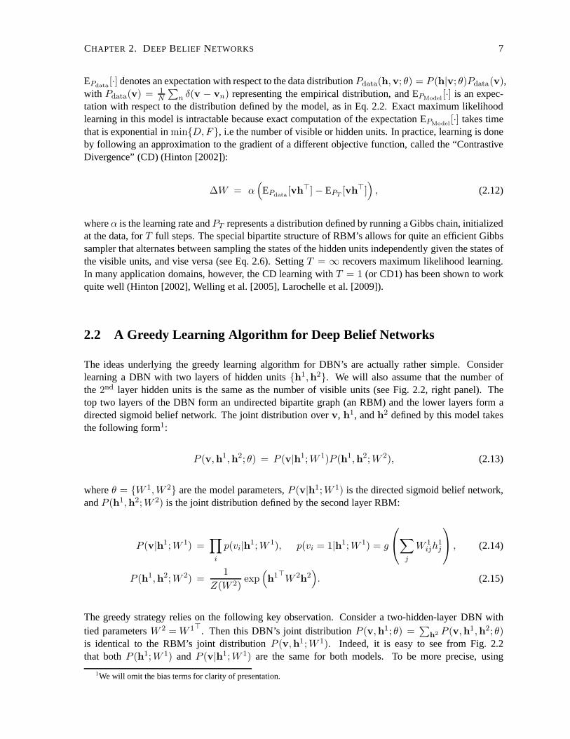
2.2 A Greedy Learning Algorithm for Deep Belief Networks
The ideas underlying the greedy learning algorithm for DBN’s are actually rather simple. Considerlearning a DBN with two layers of hidden unitsh1,h2. We will also assume that the number ofthe 2nd layer hidden units is the same as the number of visible units (see Fig. 2.2, right panel). Thetop two layers of the DBN form an undirected bipartite graph (an RBM) and the lower layers form adirected sigmoid belief network. The joint distribution over v, h1, andh2 defined by this model takesthe following form1:
P (v,h1,h2; θ) = P (v|h1;W 1)P (h1,h2;W 2), (2.13)
whereθ = W 1,W 2 are the model parameters,P (v|h1;W 1) is the directed sigmoid belief network,andP (h1,h2;W 2) is the joint distribution defined by the second layer RBM:
P (v|h1;W 1) =∏
i
p(vi|h1;W 1), p(vi = 1|h1;W 1) = g
∑
j
W 1ijh
1j
, (2.14)
P (h1,h2;W 2) =1
Z(W 2)exp
(h1⊤W 2h2
). (2.15)
The greedy strategy relies on the following key observation. Consider a two-hidden-layer DBN withtied parametersW 2 = W 1⊤. Then this DBN’s joint distributionP (v,h1; θ) =
∑h2 P (v,h1,h2; θ)
is identical to the RBM’s joint distributionP (v,h1;W 1). Indeed, it is easy to see from Fig. 2.2that bothP (h1;W 1) and P (v|h1;W 1) are the same for both models. To be more precise, using
1We will omit the bias terms for clarity of presentation.

CHAPTER 2. DEEP BELIEF NETWORKS 8
h
v
W1
h1
h2
v
W1
W1⊤
Figure 2.2:Left: Restricted Boltzmann Machine.Right: A two-hidden-layer Deep Belief Network with tiedweightsW 2 =W 1⊤. The joint distributionP (v,h1; W 1) defined by this DBN is identical to the joint distributionP (v,h1; W 1) defined by an RBM.
Eqs. 2.13, 2.14, 2.15 and the fact thatW 2 =W 1⊤, we obtain the DBN’s joint distribution:
P (v,h1; θ) = P (v|h1;W 1)×∑
h2
P (h1,h2;W 2)
=∏
i
p(vi|h1;W 1)× 1
Z(W 2)
∏
i
1 + exp
∑
j
W 2jih
1j
=∏
i
exp(vi
∑j W 1
ijh1j
)
1 + exp(∑
j W 1ijh
1j
) × 1
Z(W 2)
∏
i
1 + exp
∑
j
W 2jih
1j
=1
Z(W 1)
∏
i
exp
vi
∑
j
W 1ijh
1j
[
sinceW 2ji = W 1
ij, Z(W 1) = Z(W 2)]
=1
Z(W 1)exp
∑
ij
W 1ijvih
1j
, (2.16)
which is identical to the joint distribution defined by an RBM(Eq. 2.2).The greedy learning algorithm uses a stack of RBM’s and proceeds as follows. We first train the
bottom RBM with parametersW 1, as described in section 2.1. We then initialize the2nd layer weightsto W 2 = W 1⊤, which ensures that the two-hidden-layer DBN is at least as good as our original RBM.We can now improve the DBN’s fit to the training data by untyingand refiningW 2.
For any approximating distributionQ(h1|v), the log-likelihood of the two-hidden-layer DBN modelhas the following variational lower bound, where the statesh2 are analytically summed out:
log P (v; θ) ≥∑
h1
Q(h1|v)
[log P (v,h1; θ)
]+H(Q(h1|v))
=∑
h1
Q(h1|v)
[log P (h1;W 2) + log P (v|h1;W 1)
]+H(Q(h1|v)), (2.17)
whereH(·) is the entropy functional. We setQ(h1|v) = P (h1|v;W 1) defined by the bottom RBM
(Eq. 2.6). Initially, whenW 2 = W 1⊤, Q is the DBN’s true factorial posterior overh1, in which casethe bound is tight. The strategy of greedy learning algorithm is to freeze the parameter vectorW 1 and

CHAPTER 2. DEEP BELIEF NETWORKS 9
RBM
RBM
RBM
Deep Belief Network
Figure 2.3:Left: Greedy learning a stack of RBM’s in which the samples from thelower-level RBM are used asthe data for training the next RBM.Right: The corresponding Deep Belief Network.
Algorithm 1 Recursive Greedy Learning Procedure for the DBN.
1: Fit parametersW 1 of the1st layer RBM to data.2: Freeze the parameter vectorW 1 and use samplesh1 from Q(h1|v) = P (h1|v,W 1) as the data for
training the next layer of binary features with an RBM.3: Freeze the parametersW 2 that define the2nd layer of features and use the samplesh2 from
Q(h2|h1) = P (h2|h1,W 2) as the data for training the3rd layer of binary features.4: Proceed recursively for the next layers.
attempt to learn a better model forP (h1;W 2) by maximizing the variational lower bound of Eq. 2.17with respect toW 2. Maximizing this bound with frozenW 1 amounts to maximizing:
∑
h1
Q(h1|v) log P (h1;W 2), (2.18)
which is equivalent to maximum likelihood training of the2nd layer RBM with vectorsh1 drawn fromQ(h1|v) as data. When presented with a dataset ofN training input vectors, the2nd layer RBM,P (h1;W 2), will learn a better model of the “aggregated” posterior over h1, which is simply the mix-ture of factorial posteriors for all the training cases:1
N
∑n P (h1|vn;W 1). Note that any increase in
the variational lower bound, as a result of changingW 2, will result in an increase of the DBN’s datalikelihood2
This idea can be extended to training the3rd layer RBM on vectorsh2 drawn from the secondRBM. By initializing W 3 =W 2⊤, we are guaranteed to improve the lower bound on the log-likelihood,
2Improving the variational bound by changingW 2 from the value it initially had when the second hidden layer was createdincreases the log-likelihood because the bound is initially tight. Further changes toW 2 that increase the variational boundfurther are not guaranteed to increase the log-likelihood further, but they are guaranteed to keep it above the value it hadwhenW 2 was created. When learning deeper layers, the variational bound does not start off being tight so even the initialimprovement in the bound when the deepest weights are first modified is not guaranteed to increase the log-likelihood.

CHAPTER 2. DEEP BELIEF NETWORKS 10
...
h2 ∼ P(h2,h3)
h1 ∼ P(h1|h2)
v ∼ P(v|h1)
h3 ∼ Q(h3|h2)
h2 ∼ Q(h2|h1)
h1 ∼ Q(h1|v)
v
h3 ∼ Q(h3|v)
h2 ∼ Q(h2|v)
h1 ∼ Q(h1|v)
v
Gibbs chain
Figure 2.4: Left: Generating a sample from the Deep Belief Network.Right: Generating a sample fromapproximate posteriorQ(h1,h2,h3|v) vs. generating a sample from fully factorized approximate posteriorQ(h1|v)Q(h2|v)Q(h3|v).
Algorithm 2 Modified Recursive Greedy Learning Procedure for the DBN.
1: Fit parametersW 1 of the1st layer RBM to data.2: Freeze the parameter vectorW 1 and use samplesh1 from Q(h1|v) = P (h1|v,W 1) as the data for
training the next layer of binary features with an RBM.3: Freeze the parametersW 2 that define the2nd layer of features and use the samplesh2 from Q(h2|v)
as the data for training the3rd layer of binary features.4: Proceed recursively for the next layers.
although changingW 3 to improve the bound can decrease the actual log-likelihood. This greedy, layer-by-layer training can be repeated several times to learn a deep, hierarchical model. The procedure issummarized in Algorithm 1.
After training a DBN withL layers, the model’s joint distribution and its approximateposteriordistributionQ are given by:
P (v,h1, ...,hL) = P (v|h1)...P (hL−2|hL−1)P (hL−1,hL),
Q(h1, ...,hL|v) = Q(h1|v)Q(h2|h1)...Q(hL|hL−1).
To generate an approximate sample from the Deep Belief Network, we can run a prolonged alternatingGibbs sampler (Eq. 2.6) to generate an approximate samplehL−1 from P (hL−1,hL), defined by thetop-level RBM, followed by a “top-down” pass through the sigmoid belief network by stochasticallyactivating each lower layer in turn (see Fig. 2.4, left panel). To get an exact sample from the approximateposterior distributionQ, we can simply perform a “bottom-up” pass by stochasticallyactivating eachhigher layer in turn. The marginal distribution of the top-level hidden units of our approximate posteriorQ(hL|v) will be non-factorial and, in general, could be multimodal.However, for many practicalapplications (e.g. information retrieval) having an explicit form for Q(hL|v), which allows efficientapproximate inference, can be of crucial importance. One possible alternative is to choose the followingfully factorized approximating distributionQ:
Q(h1, ...,hL|v) =L∏
l=1
Q(hl|v), (2.19)

CHAPTER 2. DEEP BELIEF NETWORKS 11
where we define:
Q(h1|v) =∏
j
q(h1j |v), q(h1
j = 1|v) = g
(∑
i
W 1ijvi + a1
j
), and (2.20)
Q(hl|v) =∏
j
q(hlj |v), q(hl
j = 1|v) = g
(∑
i
W lijq(h
l−1i = 1|v) + al
j
), (2.21)
whereg(x) = 1/(1 + exp(−x)) and l = 2, .., L. The factorial posteriorQ(hL|v) can be obtainedby simply replacing the stochastic hidden units in bottom layers with real-valued probabilities, andthen performing a single deterministic bottom-up pass to computeq(hL
j = 1|v). This fully factorizedapproximation also suggests a modified greedy learning algorithm, summarized in Algorithm 2. In thisalgorithm the samples, used for training higher-level RBM’s, are instead sampled from a fully factorizedapproximate posteriorQ. It is important to observe that the modified algorithmdoes not guaranteetoimprove the lower bound on the log-probability of the training data. Nonetheless, this is the actualalgorithm commonly used in practice (Taylor et al. [2006], Hinton and Salakhutdinov [2006], Torralbaet al. [2008], Bengio [2009]), and we will use it in the next chapter of this thesis. The modified algorithmperforms well, particularly when a fully factorizedQ is used to perform approximate inference in thefinal model. Details of Matlab implementation of the modifiedgreedy learning algorithm can be foundin Appendix A.
In practice, however, many of the assumptions that we have tomake in order to guarantee theimprovement of the lower bound on the data likelihood are violated. In particular, the assumption thatlearning higher-level RBM’s can be carried out using maximum likelihood (see Eq. 2.18) is clearly
violated. Furthermore, when adding a new layerl, we typically do not initializeW l = W l−1⊤, whichwould force the number of hidden units of the new RBM to be the same as the number of the visibleunits of the lower level RBM3. In chapter 4 of this thesis, we will address a problem of evaluatinggeneralization performance of Deep Belief Networks as density models, which will allow us to domodel selection and complexity control.
2.3 Generalizing RBM’s to Modeling Real-valued and Count Data
Welling et al. [2005] introduced a class of two-layer undirected graphical models that generalize RBM’sto exponential family distributions. In the remaining partof this section, we will review two specificmodels: Gaussian RBM and Replicated Softmax model (Salakhutdinov and Hinton [2010]). These mod-els will allow us to model real-valued data (e.g. image patches) and count data (e.g. word-count vectorsof documents), when learning DBN’s. Other extensions include exponential or truncated exponentialRBM’s (Bengio et al. [2007]), and Poisson RBM’s (Gehler et al. [2006])
Gaussian RBM’s
Consider modeling visible real-valued unitsv ∈ RD and leth ∈ 0, 1F be binary stochastic hidden
units. The energy of the statev,h of the Gaussian RBM is defined as follows:
E(v,h; θ) =
D∑
i=1
(vi − bi)2
2σ2i
−D∑
i=1
F∑
j=1
Wijhjvi
σi−
F∑
j=1
ajhj , (2.22)
3Although if the number of hidden units per layer does not decrease, it easy to show (Hinton et al. [2006]) that adding eachnew layer guarantees to increase a lower bound on the data likelihood, provided higher-level RBM’s are trained by maximumlikelihood.
CHAPTER 2. DEEP BELIEF NETWORKS 12
Training Samples
Learned Receptive Fields
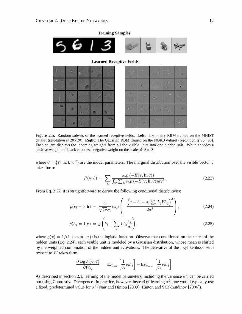
Figure 2.5: Random subsets of the learned receptive fields.Left: The binary RBM trained on the MNISTdataset (resolution is 28×28). Right: The Gaussian RBM trained on the NORB dataset (resolution is 96×96).Each square displays the incoming weights from all the visible units into one hidden unit. White encodes apositive weight and black encodes a negative weight on the scale of -3 to 3.
whereθ = W,a,b, σ2 are the model parameters. The marginal distribution over the visible vectorvtakes form:
P (v; θ) =∑
h
exp (−E(v,h; θ))∫v′
∑h
exp (−E(v,h; θ))dv′. (2.23)
From Eq. 2.22, it is straightforward to derive the followingconditional distributions:
p(vi = x|h) =1√2πσi
exp
−
(x− bi − σi
∑j hjWij
)2
2σ2i
, (2.24)
p(hj = 1|v) = g
(bj +
∑
i
Wijvi
σi
), (2.25)
whereg(x) = 1/(1 + exp(−x)) is the logistic function. Observe that conditioned on the states of thehidden units (Eq. 2.24), each visible unit is modeled by a Gaussian distribution, whose mean is shiftedby the weighted combination of the hidden unit activations.The derivative of the log-likelihood withrespect toW takes form:
∂ log P (v; θ)
∂Wij= EPdata
[1
σivihj
]− EPModel
[1
σivihj
].
As described in section 2.1, learning of the model parameters, including the varianceσ2, can be carriedout using Contrastive Divergence. In practice, however, instead of learningσ2, one would typically usea fixed, predetermined value forσ2 (Nair and Hinton [2009], Hinton and Salakhutdinov [2006]).

CHAPTER 2. DEEP BELIEF NETWORKS 13
W1
W1 W2
W2
h
v
W1
W1
W1
W2
W2
W2
W1 W2
Latent Topics
Observed Softmax Visibles Multinomial Visible
Figure 2.6: The Replicated Softmax model. The top layer represents a vector h of stochastic, binary topicfeatures and the bottom layer consists of softmax visible units,v. All visible units share the same set of weights,connecting them to the binary hidden units.Left and Middle: Two members of a Replicated Softmax family fordocuments containing two and three words.Right: A different interpretation of the Replicated Softmax model,in which M softmax units with identical weights are replaced by a single multinomial unit which is sampledMtimes.
To see what a single RBM module can learn, Fig. 2.5 shows a random subset of parametersW , alsoknown as receptive fields, learned by a standard binary and a Gaussian RBM using CD1. Observe thatboth RBM’s learn highly localized receptive fields.
Modeling Word Counts with a Family of Replicated Softmax Models
Consider an undirected graphical model that consists of onevisible layer and one hidden layer as shownin Fig. 2.6. This model is a type of Restricted Boltzmann Machine in which the visible units that areusually binary have been replaced by “softmax” units that can have one of a number of different states.Let v ∈ 1, ...,KD be a vector of visible units that takes on values in some discrete alphabet, and leth ∈ 0, 1F be binary stochastic hidden topic features. LetV be aK ×D observed indicator matrixwith vk
i = 1 if visible unit i takes on valuek. The energy of the stateV,h is defined as follows:
E(V,h) = −D∑
i=1
F∑
j=1
K∑
k=1
W kijhjv
ki −
D∑
i=1
K∑
k=1
vki bk
i −F∑
j=1
hjbj , (2.26)
whereW kij is a symmetric interaction term between visible uniti that takes on valuek, and hidden unit
j, bki is the bias of uniti that takes on valuek, andaj is the bias of hidden unitj. The conditional
distributions are given by softmax and logistic functions:
p(vki = 1|h) =
exp (bki +
∑Fj=1 hjW
kij)∑K
q=1 exp(bqi +
∑Fj=1 hjW
qij
) (2.27)
p(hj = 1|V) = g
(aj +
D∑
i=1
K∑
k=1
vki W k
ij
). (2.28)
Now suppose that for each document we create a separate RBM with as many softmax units as thereare words in the document. Assuming we can ignore the order ofthe words, all of these softmax unitscan share the same set of weights. Consider a document that containsM words. In this case, we definethe energy of the stateV,h to be:
E(V,h) = −F∑
j=1
K∑
k=1
W kj hj v
k −K∑
k=1
vkbk −M
F∑
j=1
hjbj, (2.29)

CHAPTER 2. DEEP BELIEF NETWORKS 14
wherevk =∑M
i=1 vki denotes the count for thekth word. The bias terms of the hidden units are scaled up
by the length of the document. This scaling is crucial and allows hidden units to behave sensibly whendealing with documents of different lengths. We also note that usingM softmax units with identicalweights is equivalent to having one multinomial unit which is sampledM times, as shown in Fig. 2.6.The derivative of the log-likelihood with respect to parametersW takes form:
∂ log P (V; θ)
∂W kj
= EPdata
[vkhj
]− EPModel
[vkhj
].
The weights can now be shared by the whole family of differentRBM’s that are created for documentsof different lengths. We call this the “Replicated Softmax”model ]. Learning can be performed usingContrastive Divergence.

Chapter 3
Learning Feature Hierarchies with DeepBelief Networks
This chapter presents several ideas based on greedily learning a hierarchy of features from high-dimensional,richly structured sensory input. Through extensive empirical evaluations we will attempt to address thequestion of how well Deep Belief Networks perform in variousapplication domains. All of the presentedideas will exploit the following two key properties of DBN’s. First, they can be learned efficiently fromlarge amounts of unlabeled data. Second, they can be discriminatively fine-tuned using the standardbackpropagation algorithm.
In section 3.1 we show how a Deep Belief Network can be used to extract useful feature repre-sentations that would allow us to learn a good covariance kernel for a Gaussian process. In particular,if the input data is high-dimensional and highly-structured, a Gaussian kernel applied to the top layerof extracted features in the DBN works much better than a similar kernel applied to the raw input. Insections 3.2 and 3.3 we show how the greedy learning algorithm can be used to make nonlinear au-toencoders work considerably better compared to widely used methods, such as principal componentanalysis (PCA) and singular value decomposition (SVD). We then demonstrate that these deep autoen-coders can be used to discover binary “semantic” codes that allow fast and accurate information retrieval.Finally, in section 3.4 we show how the DBN framework, using partially labeled data, can also be usedto efficiently learn a nonlinear transformation from the input space to a low-dimensional feature spacein which K-nearest neighbour classification performs well.
3.1 Learning Features for Discrimination and Regression
Many real-world applications are characterized by high-dimensional, highly-structured data with a largesupply of unlabeled data and a very limited amount of labeleddata. Applications such as informationretrieval and machine vision are examples where unlabeled data is readily available. Many models,including logistic regression, Gaussian processes, and Support Vector Machines, are discriminativemodels by nature, and within the standard regression or classification scenario, unlabeled data is ofno use. Given a set ofi.i.d. labeled input vectorsXl = xnNn=1 and their associated target labelsynNn=1 ∈ R for regression orynNn=1 ∈ −1, 1 for classification, discriminative methods modelp(yn|xn) directly. Unless some assumptions are made about the underlying distribution of the inputdataX = [Xl,Xu], unlabeled data,Xu, cannot be used. Many researchers have tried to use unlabeleddata by incorporating a model ofP (X). For classification tasks, Lawrence and Scholkopf [2001] modelP (X) as a mixture
∑yn
p(xn|yn)p(yn) and then inferp(yn|xn), Seeger [2001] attempts to learn a co-variance kernel for a Gaussian process based onP (X), and Lawrence and Jordan [2004] assume that
15

CHAPTER 3. LEARNING FEATURE HIERARCHIES WITH DEEP BELIEF NETWORKS 16
the decision boundaries should occur in regions where the data density,P (X), is low. When faced withhigh-dimensional, highly-structured data, however, noneof the existing approaches have proved to beparticularly successful.
To make use of unlabeled data, we propose to first learn a DBN model of P (X) in an entirelyunsupervised way using the fast, greedy learning algorithmintroduced in section 2.2. We then use thisdeep generative model to initialize a multilayer, nonlinear mappingF (x;W ), parameterized byW , withF : X→ Z mapping the input vectors inX into a feature spaceZ. The top-level features produced bythis mapping typically allow for a rather accurate reconstruction of the input and tend to capture a lot ofthe higher-order structure in the input data. We can now fit a discriminative model to the labeled datausing the top-level features of the DBN model as inputs. Performance can be further improved by usingbackpropagation through the DBN to discriminatively fine-tune the model parameters.
While greedily pretrained DBN’s can be used to provide inputvectors for many discriminativemethods, including logistic regression, SVM’s (Vapnik [1998], Lauer et al. [2007]), and kernel regres-sion (Benedetti [1977]), in this section we will concentrate on using a Deep Belief Network to learn acovariance kernel for a Gaussian process. In particular, weshow that the parametersW of the covari-ance kernel can be fine-tuned using the labeled data by maximizing the log probability of the labels withrespect toW .
3.1.1 Gaussian Processes for Regression and Binary Classification
Gaussian processes (GP’s) are a widely used method for Bayesian nonlinear non-parametric regressionand classification (Rasmussen and Williams [2006], Seeger [2004], Neal [1997], Rasmussen [1996]).GP’s are based on defining a covariance function that encodesprior knowledge of the smoothness ofthe underlying process that is being modeled. Because of their flexibility and computational simplicity,GP’s have been successfully used in many areas of machine learning.
Let us consider the following regression task. We are given adataset ofN i .i .d . labeled inputvectorsXl = xnNn=1 and their corresponding real-valued targetsy = ynNn=1. We are interested inthe following probabilistic regression model:
yn = f(xn) + ǫ, ǫ ∼ N (0, σ2), (3.1)
whereN (µ, σ2) denotes a Gaussian distribution with meanµ and varianceσ2. A Gaussian processregression places a zero-mean GP prior over the underlying latent functionf we are modeling, so thata-priori f |Xl ∼N (0,K), wheref = [f(x1), ..., f(xn)]T andK is the covariance matrix, whose entriesare specified by the covariance functionKij = K(xi,xj). The covariance function encodes our priornotion of the smoothness off , or the prior assumption that if two input vectors are similar according tosome distance measure, their labels should be highly correlated. In this work we will use the sphericalGaussian kernel, parameterized byα, β:
Kij = α exp
(− 1
2β(xi − xj)
⊤(xi − xj)
). (3.2)
Integrating out the function valuesf , the marginal log-likelihood takes form:
L = log P (y|Xl; θ) = −N
2log 2π − 1
2log |K + σ2I| − 1
2y⊤(K + σ2I)−1y, (3.3)
which can then be maximized with respect to the parametersθ = α, β, σ. Given a new test pointx∗,a prediction is obtained by conditioning on the observed data andθ. The distribution of the predictedvaluey∗ atx∗ takes the form:
y∗|x∗,Xl,y; θ ∼ N(k∗⊤(K + σ2I)−1y, k∗∗ − k∗⊤(K + σ2I)−1k∗ + σ2
), (3.4)

CHAPTER 3. LEARNING FEATURE HIERARCHIES WITH DEEP BELIEF NETWORKS 17
W
W
W
W
W
W
GP
Input X
target y
FeatureRepresentationF(X;W)
1
RBM
RBM2
3
1000
1000
3
RBM
2
T
T
T
10001
1000
1000
1000
1000
1000
Figure 3.1:Left: Pretraining consists of learning a stack of RBM’s.Right: After pretraining, the RBM’s areused to initialize a covariance function of the Gaussian process, which is then fine-tuned by backpropagation.
wherek∗∗ = K(x∗,x∗) andk∗ = K(x∗,Xl) is theN × 1 vector of the covariances evaluated betweenall training and a test point.
For a binary classification task, we similarly place a zero mean GP prior over the values of an under-lying latent function,f , which are then passed through the logistic functiong(x) = 1/(1+exp(−x)) todefine a priorp(yn = 1|xn) = g(f(xn)). Given a new test pointx∗, inference is done by first obtainingthe distribution overf∗ = f(x∗):
p(f∗|x∗,Xl,y; θ) =
∫p(f∗|x∗,Xl, f ; θ)P (f |Xl,y; θ)df , (3.5)
which is then used to produce a probabilistic prediction:
p(y∗ = 1|x∗,Xl,y; θ) =
∫g(f∗)p(f∗|x∗,Xl,y; θ)df∗. (3.6)
The non-Gaussian likelihood makes the integral in Eq. 3.5 analytically intractable. In our experiments,we approximate the non-Gaussian posteriorP (f |Xl,y; θ) with a Gaussian one using expectation prop-agation (Minka [2001]). For more thorough reviews and implementation details refer to Rasmussen andWilliams [2006], Seeger [2004], and Neal [1997].
3.1.2 Learning the Covariance Function for a Gaussian Process
Using the layer-by-layer learning algorithm of section 2.2, we first learn a stack of RBM’s. After learn-ing is complete, the stochastic activities of the binary units in each layer are replaced by deterministic,real-valued probabilities and the DBN is used to initializea multilayer, nonlinear mappingF (x;W ) asshown in Fig. 3.1. This learning is treated as apretraining stage that captures a lot of the higher-orderstructure in the input data and is used to define a Gaussian covariance function, parameterized byα, βandW :
Kij = α exp
(− 1
2β
(F (xi;W )− F (xj ;W )
)⊤(F (xi;W )− F (xj ;W )
)). (3.7)
The covariance kernel is initialized in an entirely unsupervised way. We can now maximize the marginallog-likelihood of Eq. 3.3 with respect to the parameters of the covariance kernelα, β,W and obser-vation noiseσ2, using the labeled training data (Rasmussen and Williams [2006], Lawrence [2004]).
CHAPTER 3. LEARNING FEATURE HIERARCHIES WITH DEEP BELIEF NETWORKS 18
32.99 −41.15 66.38−22.07 27.49 UnlabeledTraining Data Test Data
A
B
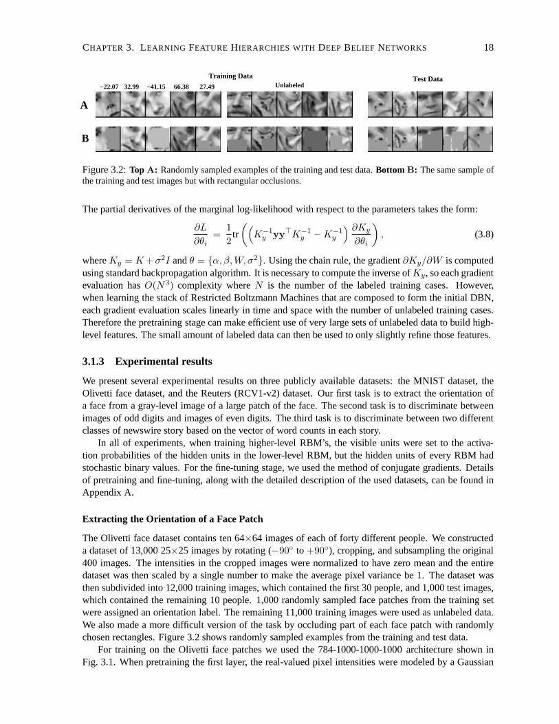
Figure 3.2:Top A: Randomly sampled examples of the training and test data.Bottom B: The same sample ofthe training and test images but with rectangular occlusions.
The partial derivatives of the marginal log-likelihood with respect to the parameters takes the form:
∂L
∂θi=
1
2tr
((K−1
y yy⊤K−1y −K−1
y
) ∂Ky
∂θi
), (3.8)
whereKy = K +σ2I andθ = α, β,W, σ2. Using the chain rule, the gradient∂Ky/∂W is computedusing standard backpropagation algorithm. It is necessaryto compute the inverse ofKy, so each gradientevaluation hasO(N3) complexity whereN is the number of the labeled training cases. However,when learning the stack of Restricted Boltzmann Machines that are composed to form the initial DBN,each gradient evaluation scales linearly in time and space with the number of unlabeled training cases.Therefore the pretraining stage can make efficient use of very large sets of unlabeled data to build high-level features. The small amount of labeled data can then be used to only slightly refine those features.
3.1.3 Experimental results
We present several experimental results on three publicly available datasets: the MNIST dataset, theOlivetti face dataset, and the Reuters (RCV1-v2) dataset. Our first task is to extract the orientation ofa face from a gray-level image of a large patch of the face. Thesecond task is to discriminate betweenimages of odd digits and images of even digits. The third taskis to discriminate between two differentclasses of newswire story based on the vector of word counts in each story.
In all of experiments, when training higher-level RBM’s, the visible units were set to the activa-tion probabilities of the hidden units in the lower-level RBM, but the hidden units of every RBM hadstochastic binary values. For the fine-tuning stage, we usedthe method of conjugate gradients. Detailsof pretraining and fine-tuning, along with the detailed description of the used datasets, can be found inAppendix A.
Extracting the Orientation of a Face Patch
The Olivetti face dataset contains ten 64×64 images of each of forty different people. We constructeda dataset of 13,000 25×25 images by rotating (−90 to +90), cropping, and subsampling the original400 images. The intensities in the cropped images were normalized to have zero mean and the entiredataset was then scaled by a single number to make the averagepixel variance be1. The dataset wasthen subdivided into 12,000 training images, which contained the first 30 people, and 1,000 test images,which contained the remaining 10 people. 1,000 randomly sampled face patches from the training setwere assigned an orientation label. The remaining 11,000 training images were used as unlabeled data.We also made a more difficult version of the task by occluding part of each face patch with randomlychosen rectangles. Figure 3.2 shows randomly sampled examples from the training and test data.
For training on the Olivetti face patches we used the 784-1000-1000-1000 architecture shown inFig. 3.1. When pretraining the first layer, the real-valued pixel intensities were modeled by a Gaussian

CHAPTER 3. LEARNING FEATURE HIERARCHIES WITH DEEP BELIEF NETWORKS 19
Training GPstandard GP-DBNgreedy GP-DBNfine GPpcalabels Sph. ARD Sph. ARD Sph. ARD Sph. ARD
A 100 22.24 28.57 17.94 18.37 15.28 15.01 18.13 (10) 16.47 (10)500 17.25 18.16 12.71 8.96 7.25 6.84 14.75 (20) 10.53 (80)1000 16.33 16.36 11.22 8.77 6.42 6.31 14.86 (20) 10.00 (160)
B 100 26.94 28.32 23.15 19.42 19.75 18.59 25.91 (10) 19.27 (20)500 20.20 21.06 15.16 11.01 10.56 10.12 17.67 (10) 14.11 (20)1000 19.20 17.98 14.15 10.43 9.13 9.23 16.26 (10) 11.55 (80)
Table 3.1:Performance results on the face-orientation regression task. The root mean squared error (RMSE) onthe test set is shown for each method using a spherical Gaussian kernel and a Gaussian kernel with ARD hyper-parameters.By row: A) Non-occluded face data, B) Occluded face data. For the GPpca model, the number ofprincipal components that performs best on the test data is shown in parenthesis.
Feature 992
Fea
ture
312
0 0.2 0.4 0.6 0.8 1.0
1.0
0.8
0.6
0.4
0.2
1 2 3 4 5 60
5
10
15
20
25
30
35
40
45
log β
−1 0 1 2 3 4 5 60
10
20
30
40
50
60
70
80
90
log β
More Relevant
Input Pixel Space
Feature Space
Figure 3.3:Left: A scatter plot of the two most relevant features, with each point replaced by the correspondinginput test image. For better visualization, overlapped images are not shown.Right: The histogram plots of thelearned ARD hyper-parameterslog β.
RBM with unit variance. The remaining RBM’s in the stack usedlogistic units. The entire training setof 12,000 unlabeled images was used for greedy, layer-by-layer training of a Deep Belief Network. Themodel contained about 2.8 million parameters, which may seem excessive for 12,000 training cases.However, each training case involves modeling 625 real-valued pixels rather than just a single real-valued target label.
After the DBN has been pretrained on the unlabeled data, a GP model was fitted to the labeleddata using the top-level features of the DBN model as inputs.We call this modelGP-DBNgreedy.GP-DBNgreedy can be further fine-tuned by maximizing the marginal log probability of the labels withrespect toW using backpropagation algorithm. We call this modelGP-DBNfine. For comparison, wefitted a GP model that used the pixel intensities of only the labeled images as its inputs. We call thismodelGPstandard. We also used PCA1 to reduce the dimensionality of the labeled images and fittedseveral different GP models using the projections onto the first m principal components as the input.
1Principal components were extracted using all 12,000 training cases.
CHAPTER 3. LEARNING FEATURE HIERARCHIES WITH DEEP BELIEF NETWORKS 20
Train GPstandard GP-DBNgreedy GP-DBNfine GPpcalabels Sph. ARD Sph. ARD Sph. ARD Sph. ARD
100 0.0884 0.1087 0.0528 0.0597 0.0501 0.0599 0.0785 (10) 0.0920 (10)500 0.0222 0.0541 0.0100 0.0161 0.0055 0.0104 0.0160 (40) 0.0235 (20)1000 0.0129 0.0385 0.0058 0.0059 0.0050 0.0100 0.0091 (40) 0.0127 (40)
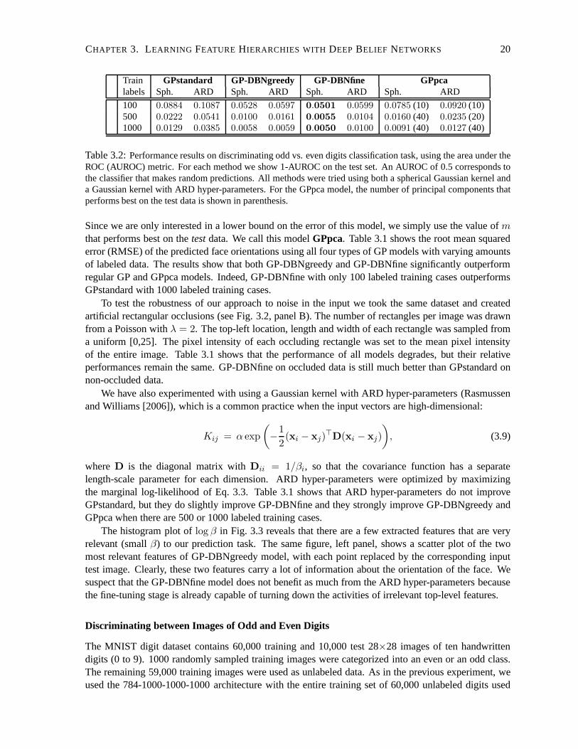
Table 3.2:Performance results on discriminating odd vs. even digits classification task, using the area under theROC (AUROC) metric. For each method we show 1-AUROC on the test set. An AUROC of 0.5 corresponds tothe classifier that makes random predictions. All methods were tried using both a spherical Gaussian kernel anda Gaussian kernel with ARD hyper-parameters. For the GPpca model, the number of principal components thatperforms best on the test data is shown in parenthesis.
Since we are only interested in a lower bound on the error of this model, we simply use the value ofmthat performs best on thetestdata. We call this modelGPpca. Table 3.1 shows the root mean squarederror (RMSE) of the predicted face orientations using all four types of GP models with varying amountsof labeled data. The results show that both GP-DBNgreedy andGP-DBNfine significantly outperformregular GP and GPpca models. Indeed, GP-DBNfine with only 100labeled training cases outperformsGPstandard with 1000 labeled training cases.
To test the robustness of our approach to noise in the input wetook the same dataset and createdartificial rectangular occlusions (see Fig. 3.2, panel B). The number of rectangles per image was drawnfrom a Poisson withλ = 2. The top-left location, length and width of each rectangle was sampled froma uniform [0,25]. The pixel intensity of each occluding rectangle was set to the mean pixel intensityof the entire image. Table 3.1 shows that the performance of all models degrades, but their relativeperformances remain the same. GP-DBNfine on occluded data isstill much better than GPstandard onnon-occluded data.
We have also experimented with using a Gaussian kernel with ARD hyper-parameters (Rasmussenand Williams [2006]), which is a common practice when the input vectors are high-dimensional:
Kij = α exp
(−1
2(xi − xj)
⊤D(xi − xj)
), (3.9)
whereD is the diagonal matrix withDii = 1/βi, so that the covariance function has a separatelength-scale parameter for each dimension. ARD hyper-parameters were optimized by maximizingthe marginal log-likelihood of Eq. 3.3. Table 3.1 shows thatARD hyper-parameters do not improveGPstandard, but they do slightly improve GP-DBNfine and theystrongly improve GP-DBNgreedy andGPpca when there are 500 or 1000 labeled training cases.
The histogram plot oflog β in Fig. 3.3 reveals that there are a few extracted features that are veryrelevant (smallβ) to our prediction task. The same figure, left panel, shows a scatter plot of the twomost relevant features of GP-DBNgreedy model, with each point replaced by the corresponding inputtest image. Clearly, these two features carry a lot of information about the orientation of the face. Wesuspect that the GP-DBNfine model does not benefit as much fromthe ARD hyper-parameters becausethe fine-tuning stage is already capable of turning down the activities of irrelevant top-level features.
Discriminating between Images of Odd and Even Digits
The MNIST digit dataset contains 60,000 training and 10,000test 28×28 images of ten handwrittendigits (0 to 9). 1000 randomly sampled training images were categorized into an even or an odd class.The remaining 59,000 training images were used as unlabeleddata. As in the previous experiment, weused the 784-1000-1000-1000 architecture with the entire training set of 60,000 unlabeled digits used

CHAPTER 3. LEARNING FEATURE HIERARCHIES WITH DEEP BELIEF NETWORKS 21
Number of labeled GPstandard GP-DBNgreedy GP-DBNfinecases (50% in each class)
100 0.1295 0.1180 0.0995500 0.0875 0.0793 0.06091000 0.0645 0.0580 0.0458
Table 3.3:Performance results using the area under the ROC (AUROC) metric on the text classification task. Foreach method we show 1-AUROC on the test set.
for greedily pretraining the DBN model. Table 3.2 shows the area under the ROC curve for discriminat-ing between odd and even digits. GP-DBNfine and GP-DBNgreedyperform considerably better thanGPstandard both with and without ARD hyper-parameters.
Classifying News Stories
The Reuters RCV1-v2 dataset is an archive of 804,414 newswire stories. The corpus covers four majorgroups: Corporate/Industrial, Economics, Government/Social, and Markets. The data was randomlysplit into 802,414 training and 2000 test articles. The testset contains 500 articles of each major group.The available data was already in a convenient, preprocessed format, where common stopwords wereremoved and all the remaining words were stemmed. We only made use of the 2000 most frequentlyused word stems in the training data. As a result, each document was represented as a vector containing2000 word counts. No other preprocessing was done.
For the text classification task we used a 2000-1000-1000-1000 architecture. The entire unlabeledtraining set of 802,414 articles was used for learning a multilayer generative model of the text docu-ments. The bottom layer of the DBN was trained using a Replicated Softmax model (see section 2.3).Table 3.3 shows the area under the ROC curve for classifying documents belonging to the Corpo-rate/Industrial vs. Economics groups. As expected, GP-DBNfine and GP-DBNgreedy work betterthan GPstandard. The results of binary discrimination between other pairs of document classes are verysimilar to the results presented in table 3.3. Our experiments using a Gaussian kernel with ARD hyper-parameters did not show any significant improvements. Examining the histograms of the length-scaleparametersβ, we found that most of the input word-counts as well as most ofthe extracted featureswere relevant to the classification task.
3.1.4 Discussion
We have shown how to greedily pretrain and discriminativelyfine-tune a covariance kernel for a Gaus-sian process. For high-dimensional, highly-structured input, this is a very effective way to make use oflarge unlabeled datasets, especially when labeled training data is scarce. The performance of pretrainedand fine-tuned GP models further reveals that the learned high-level feature representations capture a lotof structure in the unlabeled input data, which is useful forsubsequent classification or regression tasks,even though these tasks are unknown when the deep generativemodel is being trained.
The same framework can also be used to discover useful low-dimensional representations of high-dimensional data, which can be used for exploratory data analysis, preprocessing, and data visualization.We explore this idea in the next section.
3.2 Nonlinear Dimensionality Reduction
Scientists working with large amounts of high-dimensionaldata are constantly facing the problem ofdimensionality reduction: how to discover low-dimensional structure from high-dimensional observa-

CHAPTER 3. LEARNING FEATURE HIERARCHIES WITH DEEP BELIEF NETWORKS 22
W
W
W +ε
W
W
W
W
W +ε
W +ε
W +ε
W
W +ε
W +ε
W +ε
+ε
W
W
W
W
W
W
1
2000
RBM
2
2000
1000
500
500
1000
1000
500
1 1
2000
2000
500500
1000
1000
2000
500
2000
T
4T
RBM
Pretraining Unrolling
1000 RBM
3
4
30
30
Fine−tuning
4 4
2 2
3 3
4T
5
3T
6
2T
7
1T
8
Encoder
1
2
3
30
4
3
2T
1T
Code layer
Decoder
RBMTop
Figure 3.4: Pretraining consists of learning a stack of Restricted Boltzmann Machines each having only onelayer of feature detectors. The learned feature activations of one RBM are used as the “data” for training the nextRBM in the stack. After the pretraining, the RBM’s are “unrolled” to create a deep autoencoder, which is thenfine-tuned using backpropagation of error derivatives.
tions. There exist a variety of dimensionality reduction techniques, which can be broadly classified into:linear methods, such as principal component analysis (PCA), nonlinear mappings, such as autoencoders(Plaut and Hinton [1987], DeMers and Cottrell [1993]), and proximity based methods, such as LocalLinear Embedding (Roweis and Saul [2000]).
Most of the existing algorithms suffer from various drawbacks. If the data lie on an embedded low-dimensional nonlinear manifold, then linear methods, eventhough computationally efficient, cannotrecover this structure as well as their nonlinear counterparts. Proximity based methods are more power-ful, but their computational cost scales quadratically with the number of observations, so they generallycannot be applied to very large high-dimensional datasets.Nonlinear mapping algorithms, such as au-toencoders, are generally painfully slow to train, and are prone to getting stuck in local minima.
3.2.1 Pretraining Autoencoders
The standard way to train autoencoders is to use backpropagation to reduce the reconstruction error.As we show, it is generally very difficult to optimize nonlinear autoencoders that have multiple hiddenlayers with hundreds of thousands of parameters (DeMers andCottrell [1993], Hecht-Nielsen [1995],Larochelle et al. [2009]). This is perhaps the main reason why this potentially powerful dimensionalityreduction algorithm has not found its applications in practice. Instead, we will use the greedy learningalgorithm to pretrain autoencoders, by learning a stack of RBM’s, as shown in Fig. 3.4. The key ideais that the greedy learning algorithm can quickly find parameters that already produce a good datareconstruction model.
After the pretraining stage, which is similar to the construction defined in subsection 3.1.2, thestochastic activities of the binary features in each layer are replaced by deterministic, real-valued proba-bilities and the model is “unrolled” to produce encoder and decoder networks. Initially both the encoderand decoder networks share the same set of weights. The global fine-tuning stage then slightly refinesthe weights for optimal reconstruction by using backpropagation of error derivatives through the whole

CHAPTER 3. LEARNING FEATURE HIERARCHIES WITH DEEP BELIEF NETWORKS 23
a)
b)
c)
d)
e)
a)
b)
c)
d)
Figure 3.5:Left Panel (by row): a) Random samples of curves from the test dataset;b) reconstructions producedby the 6-dimensional deep autoencoder;c) reconstructions by “logistic PCA” using6 components;d) reconstruc-tions by logistic ande) standard PCA using18 components. The average squared error per image for the lastfour rows is1.44, 7.64, 2.45, 5.90. Right panel (by row): a) A random MNIST test image from each class;b) reconstructions by the 30-dimensional autoencoder;c) reconstructions by 30-dimensional logistic PCA and d)standard PCA. The average squared errors for the last three rows are3.00, 8.01, and13.87.
autoencoder.
3.2.2 Experimental results
In all our experiments, when pretraining deep autoencoders, the top level RBM was a Gaussian RBM,as described in section 2.3, but with visible and hidden units switched. So the hidden units of the toplevel RBM were modeled by a unit variance Gaussian distribution, whose mean was determined bythe weighted combination of the binary visible units. This allowed the low-dimensional codes to makegood use of continuous variables and facilitated comparisons with PCA. Description of the datasets,along with details of software that we used for pretraining and fine-tuning deep autoencoders, can befound in Appendix A.
Synthetic curves dataset
To evaluate the two-stage learning procedure, we first used asynthetic curves dataset that contains28×28 images of “curves”, generated from three randomly chosen2-dimensional points. For thisdataset, the true intrinsic dimensionality of data is six, but the relationship between the pixel intensitiesand the six numbers used to generate them is highly nonlinear. The pixel intensities were normalizedto lie in the interval[0, 1] (see Fig. 3.5, left panel). The intensities had a tendency tomostly take onextreme values, and therefore were modeled in the first layerby a standard binary RBM. During thefine-tuning stage, we minimized the cross-entropy error:
E = −∑
i
pi log pi −∑
i
(1− pi) log(1− pi), (3.10)
wherepi is the intensity of pixeli andpi is the intensity of its reconstruction.We used a deep autoencoder that consisted of an encoder with layers of size (28×28)-400-200-100-
50-25-6 and a symmetric decoder. This is probably much deeper than is necessary for this task, butone of the points of this experiment was to demonstrate that we could train very deep networks. The6 units in the code layer were linear and all the other units were logistic. The autoencoder was trainedon 20,000 images and tested on 10,000 new images. Figure 3.5 shows that the autoencoder was able todiscover the nonlinear mapping between 784 pixel image and 6real numbers that allow almost perfectreconstruction. PCA, on the other hand, gives considerablyworse results. Figure 3.5 also compares

CHAPTER 3. LEARNING FEATURE HIERARCHIES WITH DEEP BELIEF NETWORKS 24
50 100 150 200 250 300 350 400 450 5000
2
4
6
8
10
12
14
16
18
20
Number of Epochs
Squ
ared
Rec
onst
ruct
ion
Err
or
Pretrained Autoencoder
Randomly Initialized Autoencoder
50 100 150 200 250 300 350 400 450 5000
0.5
1
1.5
2
2.5
3
3.5
4
4.5
5
Number of Epochs
Squ
ared
Rec
onst
ruct
ion
Err
or
Pretrained Autoencoder
Randomly Initialized Autoencoder
50 100 150 200 250 300 350 400 450 5001
1.5
2
2.5
3
3.5
4
Number of Epochs
Squ
ared
Rec
onst
ruct
ion
Err
or
Pretrained Shallow Autoencoder
Pretrained Deep Autoencoder
Figure 3.6: The average squared reconstruction error per test image during fine-tuning on the curves train-ing data. Left: The deep 784-400-200-100-50-25-6 autoencoder makes rapidprogress after pretraining but noprogress without pretraining.Middle: A shallow 784-532-6 autoencoder can learn without pretraining but pre-training makes the fine-tuning much faster.Right: A 784-100-50-25-6 autoencoder performs slightly better thana shallower 784-108-6 autoencoder that has about the same number of parameters. Both autoencoders were pre-trained.
a)
b)
c)
Figure 3.7:By row: a) Random samples from the test dataset;b) reconstructions by the 30-dimensional autoen-coder; andc) reconstructions by 30-dimensional PCA. The average squared errors are 126 and 135.
our deep nonlinear autoencoder to a shallow linear autoencoder, which we call logistic PCA, where thelinear code units are directly connected to both the inputs and the logistic output units.
Figure 3.6, left panel, shows performance of pretrained andrandomly initialized deep autoencoderson the curves dataset. Note that without pretraining, the deep autoencoder gets stuck at poor localoptimum. It always reconstructs the average of the trainingdata, even after prolonged fine-tuning.Shallow autoencoders can learn without pretraining, but pretraining greatly reduces the total trainingtime. Figure 3.6, right panel, further reveals that when thenumber of parameters is the same, a deepautoencoder produces a slightly lower reconstruction error on test data than a shallow autoencoder.
MNIST and Olivetti datasets
We used a (28×28)-1000-500-250-30 autoencoder to extract 30-dimensional codes of the handwrittendigits in the MNIST training set. Similar to the curves dataset, all units were logistic except for the 30linear units in the code layer. After fine-tuning on all 60,000 training images using cross-entropy error,the autoencoder was tested on 10,000 new images. Figure 3.5 shows that the deep autoencoder capturesthe structure of the data much better than logistic PCA, which, in turn, is much better than standardPCA. Figure 3.8 also shows that a two-dimensional autoencoder produces a much better visualizationof the data compared to the first two principal components of PCA.
We then used a (25×25)-2000-1000-500-30 autoencoder with linear input unitsto discover 30-

CHAPTER 3. LEARNING FEATURE HIERARCHIES WITH DEEP BELIEF NETWORKS 25
0123456789
Figure 3.8:Left : The 2-D codes for 500 digits of each class produced by takingthe first two principal compo-nents of all 60,000 training images.Right: The 2-D codes discovered by a 784-1000-500-250-2 autoencoder.
0.1 0.2 0.4 0.8 1.6 3.2 6.4 12.8 25.6 51.2 100
10
20
30
40
50
Recall (%)
Pre
cisi
on (
%)
Autoencoder 10DLSA 10DLSA 50DAutoencoder 10Dprior to fine−tuning
Figure 3.9:Precision-Recall curves for the Reuters RCV1-v2 dataset, when a query document from the test setis used to retrieve other test set documents, averaged over all 402,207 possible queries.
dimensional codes for grey-level image patches that were derived from the Olivetti face dataset. Adataset of 165,600 25×25 images was created by randomly rotating (−90 to +90), scaling (1.4 to1.8), cropping, and subsampling the original 400 images. The dataset was then subdivided into 124,200training images, which contained the first thirty people, and 41,400 test images, which contained the re-maining ten people. Figure 3.5, bottom panel, shows that thethe 30-dimensional autoencoder producesmuch better reconstructions than 30-dimensional PCA.
Reuters Corpus
We can also use autoencoders to discover low-dimensional codes that would allow for fast document re-trieval. We performed a set of experiments on Reuters RCV1-v2 dataset that contains 804,414 newswire

CHAPTER 3. LEARNING FEATURE HIERARCHIES WITH DEEP BELIEF NETWORKS 26
Legal/JudicialLeading Economic Indicators
European Community Monetary/Economic
Accounts/Earnings
Interbank Markets
Government Borrowings
Disasters and Accidents
Energy Markets
Autoencoder 2-D Code SpaceLSA 2-D Code Space
Figure 3.10:Left : The codes produced by the 2-dimensional LSA.Right: The codes produced by a 2000-500-250-125-2 autoencoder.
stories, manually categorized into 103 topics. The data wassplit randomly into 402,212 training and402,212 test documents. We trained a 2000-500-250-125-10 autoencoder, where each document wasrepresented as a vector containing 2000 most frequently used words in the training dataset. When pre-training the first layer, the word-count vectors were modelled by the Replicated Softmax model. For thefine-tuning stage, we divided the count vector by the number of words, so that it represented a probabil-ity distribution across words, and then used the cross-entropy error function with a softmax at the outputlayer. Figure 3.9 shows that when we use the cosine of the angle between two codes to measure sim-ilarity, the autoencoder significantly outperforms LatentSemantics Analysis (LSA) (Deerwester et al.[1990]), a well-known document retrieval method based on singular value decomposition. Even priorto fine-tuning, the autoencoder outperforms LSA. Figure 3.10 further shows that the two-dimensionalcodes produced an autoencoder are much better organized, compared to the codes produced by LSA.
3.2.3 Discussion
Together with pretraining, nonlinear autoencoders can be very effective for nonlinear dimensionalityreduction. Unlike non-parametric methods, such as LLE (Roweis and Saul [2000]), ISOMAP (Tenen-baum et al. [2000]), or t-SNE (van der Maaten and Hinton [2009]), autoencoders provide mappingsin both directions between the data and code spaces. They canalso be applied to very large datasets,because both the pretraining and fine-tuning scale linearlyin time and space with the number of trainingcases. In the next section we show how a network with multiplelayers and with hundreds of thousandsof parameters can be trained to discover “semantic” binary codes, so that similar input vectors will havesimilar binary codewords. This, in turn, will allow us to very quickly and accurately retrieve a set ofdocuments that are similar to a given query document.
CHAPTER 3. LEARNING FEATURE HIERARCHIES WITH DEEP BELIEF NETWORKS 27
3.3 Document Retrieval
One of the most popular and widely used algorithms for retrieving documents that are similar to aquery document is TF-IDF (Salton and Buckley [1988], Salton[1991]), which measures the similaritybetween documents by comparing their word-count vectors. The similarity metric weights each wordby both its frequency in the query document (Term Frequency)and the logarithm of the reciprocal of itsfrequency in the whole set of documents (Inverse Document Frequency). TF-IDF, however, has severalmajor limitations: it computes document similarity directly in the word-count space, and it assumes thatthe counts of different words provide independent evidenceof similarity.
To remedy these drawbacks, numerous models for capturing low-dimensional, latent representa-tions have been proposed and successfully applied in the domain of information retrieval. A simpleand widely-used method is Latent Semantic Analysis (LSA) (Deerwester et al. [1990]), which extractslow-dimensional semantic structure using SVD decomposition to get a low-rank approximation of theword-document co-occurrence matrix. This allows documentretrieval to be based on “semantic” con-tent rather than just on individually weighted words. LSA, however, is very restricted in the types ofsemantic content it can capture because it is a linear method, so it can only capture pairwise correlationsbetween words. A probabilistic version of LSA (pLSA) was introduced by Hofmann [1999], using theassumption that each word is modeled as a sample from a document-specific multinomial mixture ofword distributions. A proper generative model at the level of documents, Latent Dirichlet Allocation,was introduced by Blei et al. [2003].
These probabilistic models can be viewed as graphical models in which hidden topic variables havedirected connections to variables that represent word-counts. Their major drawback is that exact infer-ence is intractable due to explaining away, so they have to resort to slow or inaccurate approximationsto compute the posterior distribution over topics. This makes it difficult to fit the models to data. Also,as Welling et al. [2005] point out, fast inference is important for information retrieval. To achieve this,they introduce a class of two-layer undirected graphical models that generalize Restricted BoltzmannMachines (RBM’s) to exponential family distributions. This allows them to model non-binary dataand to use non-binary latent variables. Maximum likelihoodlearning is intractable in these models,but learning can still be performed by using Contrastive Divergence (Hinton [2002]). Several furtherdevelopments of these undirected models (Gehler et al. [2006], Xing et al. [2005]) show that they arecompetitive in terms of retrieval accuracy with their directed counterparts.
All of the above models, however, have several important limitations. First, there are limitations onthe types of structure that can be represented efficiently bya single layer of hidden variables. We havealready seen in section 3.2 that a network with many hidden layers and with hundreds of thousands ofparameters can discover latent representations that work much better for information retrieval. Second,many of the existing retrieval algorithms are based on computing a similarity measure between a querydocument and other documents in the collection. The similarity is computed either directly in the wordspace or in a low-dimensional latent space. Typically, the larger the size of document collection, thelonger it will take to search for relevant documents.
3.3.1 Semantic Hashing
Using the two-stage learning procedure, introduced in section 3.2, we can build an autoencoder thatlearns to map documents into “semantic” binary codes. We call this model Semantic Hashing. Byusing learned binary codes as memory addresses, we can effectively learn asemantic address space,so a document can be mapped to a memory address in such a way that a small hamming-ball aroundthat memory address contains semantically similar documents, as shown in Fig. 3.11, left panel. Thisrepresentation will allow us to retrieve a short-list of semantically similar documents on very large

CHAPTER 3. LEARNING FEATURE HIERARCHIES WITH DEEP BELIEF NETWORKS 28
SemanticallySimilarDocuments
Document
Address Space
SemanticHashingFunction
0 0.1 0.2 0.3 0.4 0.5 0.6 0.7 0.8 0.9 10
1
2
3
4
5
6
7x 10
5
Activation Probabilities
Pretrained
0 0.1 0.2 0.3 0.4 0.5 0.6 0.7 0.8 0.9 10
1
2
3
4
5
6
7x 10
5
Activation Probabilities
Fine−tuned
Figure 3.11:Left : A schematic representation of Semantic Hashing.Right: The distribution of the activitiesof the 128 code units on the 20-newsgroups training data before and after fine-tuning with backpropagation anddeterministic noise.
document sets in time independent of the number of documents. The short-list can then be given to aslower but more precise retrieval method, such as TF-IDF.
Making the codes binary
During the pretraining stage, the bottom layer RBM is trained using a Replicated Softmax model, whilethe remaining RBM’s in the stack use logistic units. During the fine-tuning, we want to find codes thatare good at reconstructing the data but are as close to binaryas possible. To make the codes binary, weadd Gaussian noise to the bottom-up input received by each code unit2. Let us assume that the outputof the decoder network is not very sensitive to small changesin the output of a code unit. Then thebest way to communicate information in the presence of addednoise is to make the bottom-up inputreceived by a code unit be either very large and negative or very large and positive. Figure 3.11, rightpanel, shows that this is what the fine-tuning does.
To prevent the added Gaussian noise from messing up the conjugate gradient fine-tuning, we used“deterministic noise” with mean zero and standard deviation 4, chosen by cross-validation. For eachtraining case, the sampled noise values are fixed in advance and do not change during training. Afterfine-tuning, the codes were thresholded to produce binary code vectors. The asymmetry between0 and1 in the energy function of an RBM causes the unthresholded codes to have many more values near0 than near1, so we used a threshold of0.1. We also experimented with various values for the noisevariance and the threshold. Our results are fairly robust tovariations in these parameters and also tovariations in the number of layers and the number of units in each layer.
3.3.2 Experimental Results
To evaluate performance of our model on an information retrieval task we use Precision-Recall curves,where we define:
Recall =Number of retrieved relevant documentsTotal number of all relevant documents
Precision=Number of retrieved relevant documents
Total number of retrieved documents2We tried other ways of encouraging the code units to be binary, such as penalizing the entropy
−p log p − (1 − p) log (1 − p) for each code unit, but Gaussian noise worked better.
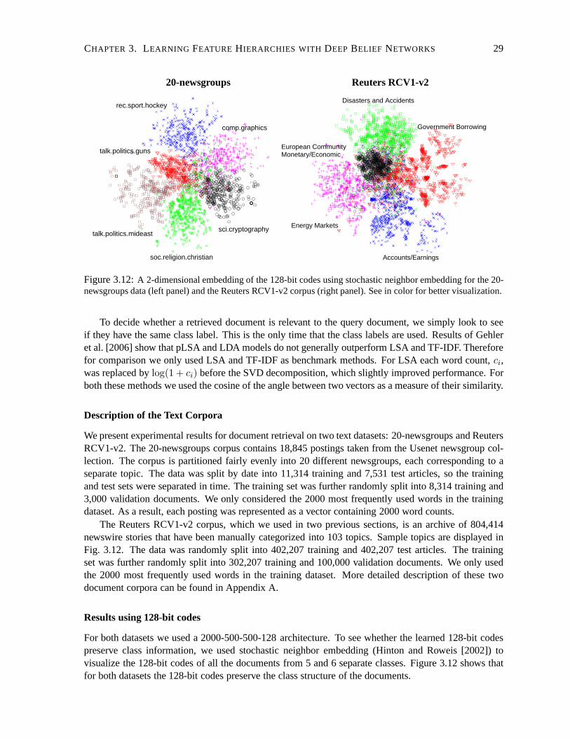
CHAPTER 3. LEARNING FEATURE HIERARCHIES WITH DEEP BELIEF NETWORKS 29
comp.graphics
rec.sport.hockey
sci.cryptography
soc.religion.christian
talk.politics.guns
talk.politics.mideast
Accounts/Earnings
Government Borrowing
European Community Monetary/Economic
Disasters and Accidents
Energy Markets
20-newsgroups Reuters RCV1-v2
Figure 3.12:A 2-dimensional embedding of the 128-bit codes using stochastic neighbor embedding for the 20-newsgroups data (left panel) and the Reuters RCV1-v2 corpus(right panel). See in color for better visualization.
To decide whether a retrieved document is relevant to the query document, we simply look to seeif they have the same class label. This is the only time that the class labels are used. Results of Gehleret al. [2006] show that pLSA and LDA models do not generally outperform LSA and TF-IDF. Thereforefor comparison we only used LSA and TF-IDF as benchmark methods. For LSA each word count,ci,was replaced bylog(1 + ci) before the SVD decomposition, which slightly improved performance. Forboth these methods we used the cosine of the angle between twovectors as a measure of their similarity.
Description of the Text Corpora
We present experimental results for document retrieval on two text datasets: 20-newsgroups and ReutersRCV1-v2. The 20-newsgroups corpus contains 18,845 postings taken from the Usenet newsgroup col-lection. The corpus is partitioned fairly evenly into 20 different newsgroups, each corresponding to aseparate topic. The data was split by date into 11,314 training and 7,531 test articles, so the trainingand test sets were separated in time. The training set was further randomly split into 8,314 training and3,000 validation documents. We only considered the 2000 most frequently used words in the trainingdataset. As a result, each posting was represented as a vector containing 2000 word counts.
The Reuters RCV1-v2 corpus, which we used in two previous sections, is an archive of 804,414newswire stories that have been manually categorized into 103 topics. Sample topics are displayed inFig. 3.12. The data was randomly split into 402,207 trainingand 402,207 test articles. The trainingset was further randomly split into 302,207 training and 100,000 validation documents. We only usedthe 2000 most frequently used words in the training dataset.More detailed description of these twodocument corpora can be found in Appendix A.
Results using 128-bit codes
For both datasets we used a 2000-500-500-128 architecture.To see whether the learned 128-bit codespreserve class information, we used stochastic neighbor embedding (Hinton and Roweis [2002]) tovisualize the 128-bit codes of all the documents from 5 and 6 separate classes. Figure 3.12 shows thatfor both datasets the 128-bit codes preserve the class structure of the documents.
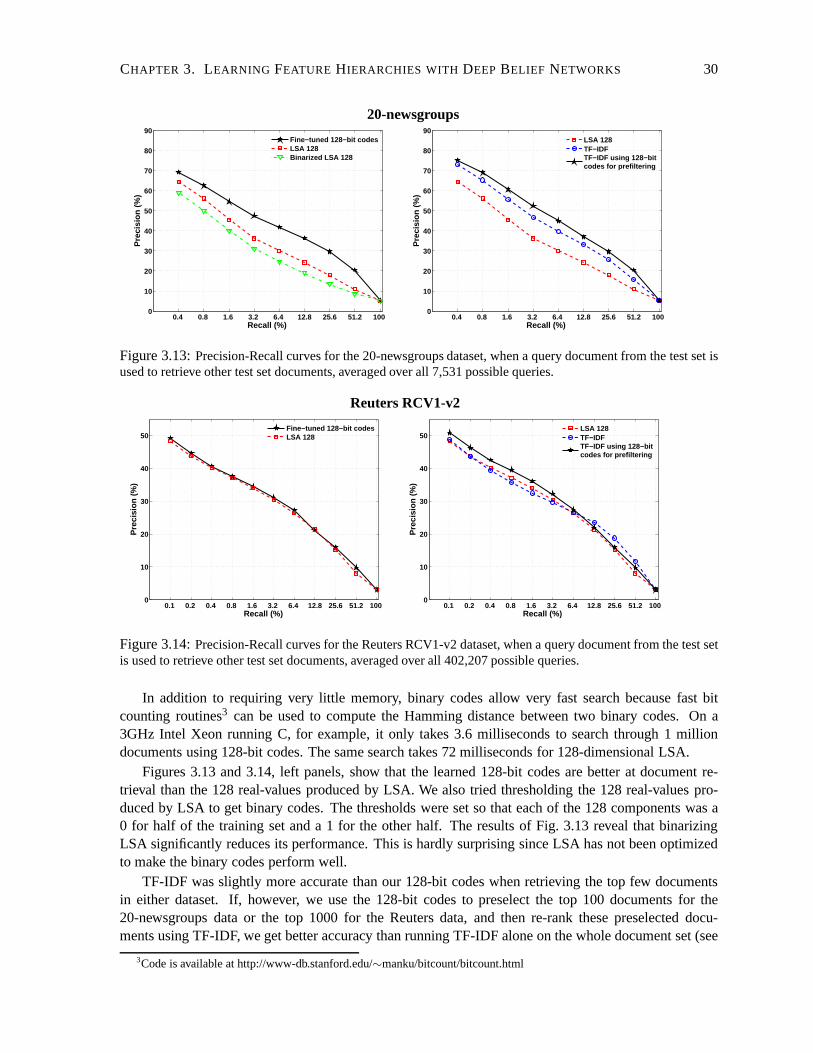
CHAPTER 3. LEARNING FEATURE HIERARCHIES WITH DEEP BELIEF NETWORKS 30
0.4 0.8 1.6 3.2 6.4 12.8 25.6 51.2 100 0
10
20
30
40
50
60
70
80
90
Recall (%)
Pre
cisi
on (
%)
Fine−tuned 128−bit codesLSA 128Binarized LSA 128
0.4 0.8 1.6 3.2 6.4 12.8 25.6 51.2 100 0
10
20
30
40
50
60
70
80
90
Recall (%)
Pre
cisi
on (
%)
LSA 128TF−IDFTF−IDF using 128−bitcodes for prefiltering
20-newsgroups
Figure 3.13:Precision-Recall curves for the 20-newsgroups dataset, when a query document from the test set isused to retrieve other test set documents, averaged over all7,531 possible queries.
0.1 0.2 0.4 0.8 1.6 3.2 6.4 12.8 25.6 51.2 100 0
10
20
30
40
50
Recall (%)
Pre
cisi
on (
%)
Fine−tuned 128−bit codesLSA 128
0.1 0.2 0.4 0.8 1.6 3.2 6.4 12.8 25.6 51.2 100 0
10
20
30
40
50
Recall (%)
Pre
cisi
on (
%)
LSA 128TF−IDFTF−IDF using 128−bitcodes for prefiltering
Reuters RCV1-v2
Figure 3.14:Precision-Recall curves for the Reuters RCV1-v2 dataset, when a query document from the test setis used to retrieve other test set documents, averaged over all 402,207 possible queries.
In addition to requiring very little memory, binary codes allow very fast search because fast bitcounting routines3 can be used to compute the Hamming distance between two binary codes. On a3GHz Intel Xeon running C, for example, it only takes 3.6 milliseconds to search through 1 milliondocuments using 128-bit codes. The same search takes 72 milliseconds for 128-dimensional LSA.
Figures 3.13 and 3.14, left panels, show that the learned 128-bit codes are better at document re-trieval than the 128 real-values produced by LSA. We also tried thresholding the 128 real-values pro-duced by LSA to get binary codes. The thresholds were set so that each of the 128 components was a0 for half of the training set and a 1 for the other half. The results of Fig. 3.13 reveal that binarizingLSA significantly reduces its performance. This is hardly surprising since LSA has not been optimizedto make the binary codes perform well.
TF-IDF was slightly more accurate than our 128-bit codes when retrieving the top few documentsin either dataset. If, however, we use the 128-bit codes to preselect the top 100 documents for the20-newsgroups data or the top 1000 for the Reuters data, and then re-rank these preselected docu-ments using TF-IDF, we get better accuracy than running TF-IDF alone on the whole document set (see
3Code is available at http://www-db.stanford.edu/∼manku/bitcount/bitcount.html

CHAPTER 3. LEARNING FEATURE HIERARCHIES WITH DEEP BELIEF NETWORKS 31
0.1 0.2 0.4 0.8 1.6 3.2 6.4 12.8 25.6 51.2 100 0
10
20
30
40
50
Recall (%)
Pre
cisi
on (
%)
TF−IDFTF−IDF using 20 bitsTF−IDF using 20 bitsand 128 bitsLocally Sensitive Hashing
Accounts/Earnings
Government Borrowing
European Community Monetary/Economic
Disasters and Accidents
Energy Markets
Reuters RCV1-v2
Figure 3.15: Left: Precision-Recall curves for the Reuters RCV1-v2 dataset, when a query document fromthe test set is used to retrieve other test set documents, averaged over all 402,207 possible queries.Right: A2-dimensional embedding of the 20-bit codes using stochastic neighbor embedding for the Reuters RCV1-v2corpus.
Figs. 3.13 and 3.14, right panels). This means that some documents that TF-IDF would have considereda very good match to the query document have been correctly eliminated by using the 128-bit codes asa filter.
Results using 20-bit codes
Using 20-bit codes, we also checked whether our learning procedure could discover a way to modelsimilarity of count-vectors by similarity of 20-bit codewords that was good enough to allow high pre-cision and retrieval for our set of 402,207 test documents. After learning to assign 20-bit addresses tothe training documents, we compute the 20-bit address of each test document and place a pointer to thedocument at its address.4
For the 402,207 test documents, a 20-bit address space givesa density of about 0.4 documents peraddress. For a given query document, we compute its 20-bit address and then retrieve all of the docu-ments stored in a hamming ball of radius 4 (about6196 × 0.4 ≅ 2500 documents) without performingany search at all. Figure 3.15 shows that neither precision nor recall is lost by restricting TF-IDF to thisfixed, preselected set.
Using a simple implementation of Semantic Hashing in C, it takes about 0.5 milliseconds to createthe short-list of about 3000 semantically similar documents (hamming-ball of radius 4) and about 0.01seconds to retrieve the top few matches from that short-listusing TF-IDF. Locality Sensitive Hashing(LSH) (Datar et al. [2004], Andoni and Indyk [2006]) takes about 0.5 seconds to perform the samesearch using E2LSH 0.1 software, provided by Alexandr Andoni and Piotr Indyk. Also, LSH is an ap-proximation to nearest-neighbor matching in the word-count space, so it cannot be expected to performbetter than TF-IDF and it generally performs slightly worse. Figure 3.15 shows that using Seman-tic Hashing as a filter, in addition to being much faster, achieves higher accuracy than either LSH orTF-IDF applied to the whole document set.
We can also use a two-stage filtering procedure by first retrieving documents using 20-bit addressesin a hamming ball of larger radius 6 (about 24317 documents),filter these down to 1000 using 128-
4We actually start with a pointer tonull at all addresses and then replace it by a one-dimensional array that contains pointersto all the documents that have that address.

CHAPTER 3. LEARNING FEATURE HIERARCHIES WITH DEEP BELIEF NETWORKS 32
bit codes, and then apply TF-IDF. This two-stage method achieves higher precision and better recallcompared to a single stage Semantic Hashing as shown in Fig. 3.15.
Semantic Hashing for Large Document Collections
For a billion documents, a 30-bit address space gives a density of about 1 document per address andSemantic Hashing only requires a few Gigabytes of memory. Using a hamming-ball of radius 5 aroundthe address of a query document, we can create a long “shortlist” of about 175,000 similar documentswith no search at all. The items in the long shortlist could befurther filtered using, for example, 128-bitbinary codes produced by an autoencoder. Using stochastic gradient descent, scaling up the learning toa billion training cases would not be particularly difficult. Indeed, Semantic Hashing has already beenscaled up and successfully applied to large image retrievaltasks that use 13 million images downloadedfrom the web (Torralba et al. [2008]).
3.3.3 Discussion
By treating the learned binary codes as memory addresses, wecan find semantically similar documentsin a time that is independent of the size of the document collection. Our results show that using usingSemantic Hashing as a filter for TF-IDF, we can achieve higherprecision and recall than TF-IDF orLocality Sensitive Hashing applied to the whole document collection.
One additional way to improve model performance is to regularize the code space using label in-formation when it is available. This can be accomplished by forcing the codes for data points of thesame label to lie close to each other in the code space, which leads to the idea of supervised learning ofnonlinear mappings.
3.4 Learning Nonlinear Mappings that Preserve Class NeighbourhoodStructure
Learning a similarity measure or distance metric over the input spaceX is an important task in machinelearning. A good similarity measure can provide insight into how high-dimensional data is organizedand it can significantly improve the performance of algorithms like K-nearest neighbours (KNN) thatare based on computing distances (Cover and Hart [1967]).
For any given distance metricD (e.g. Euclidean) we can measure similarity between two inputvectorsxi, xj ∈ X by computingD[F (xi;W ), F (xj ;W )], whereF (x;W ) is a functionF : X → Z
mapping the input vectors inX into a feature spaceZ. As noted by Globerson and Roweis [2005],learning a similarity measure is closely related to the problem of feature extraction, since for any fixedD, any feature extraction algorithm can be thought of as learning a similarity metric. Previous workstudied the case whenD is Euclidean distance andF (x;W ) is a simple linear projectionF (x;W ) =Wx. The Euclidean distance in the feature space is then the Mahalanobis distance in the input space:
D[F (xi), F (xj)] = (xi − xj)⊤ W⊤W (xi − xj) . (3.11)
Linear discriminant analysis (LDA) learns the matrixW that minimizes the ratio of within-classdistances to between-class distances. Goldberger et al. [2004] learned the linear transformation thatoptimized the performance of KNN in the resulting feature space. This differs from LDA because itallows two members of the same class to be far apart in the feature space as long as each member ofthe class is close to K other class members. Globerson and Roweis [2005] learned the matrixW suchthat the input vectors from the same class mapped to a tight cluster. They showed that their method

CHAPTER 3. LEARNING FEATURE HIERARCHIES WITH DEEP BELIEF NETWORKS 33
approximates the local covariance structure of the data andis not based on a Gaussian assumption asopposed to LDA that uses the global covariance structure. Weinberger et al. [2005] also learnedW withthe twin goals of making the K-nearest neighbours belong to the same class and making examples fromdifferent classes be separated by a large margin. They succeeded in achieving a test error rate of 1.3%on the MNIST dataset.
A linear transformation has a limited number of parameters and it cannot model higher-order cor-relations between the original data dimensions. As shown insections 3.2 and 3.3, using a nonlineartransformation functionF (x;W ), we can discover low-dimensional representations that work muchbetter than existing linear methods provided the dataset islarge enough to allow the parameters to beestimated. Using greedy unsupervised learning algorithm,we can train a multilayer, nonlinear encodernetwork that transforms the input data vectorx into a low-dimensional feature representationF (x;W ).After the initial pretraining, the parameters can be fine-tuned by performing gradient descent in theNeighbourhood Component Analysis (NCA) objective function, introduced by Goldberger et al. [2004].The learning results in a nonlinear transformation of the input space that has been optimized to makeKNN perform well in the low-dimensional feature space.
3.4.1 Learning Nonlinear NCA
We are given a set ofN labeled training cases(xi, ci), i = 1, 2, ...,N , wherexi ∈ RD, andci ∈
1, 2, ..., C. For each training vectorxi, define the probability that pointi selects one of its neighboursj in the transformed feature space as:
pij =exp (−d2
ij)∑z 6=i exp (−d2
iz), pii = 0. (3.12)
We focus on the Euclidean distance metric:
dij = ‖ F (xi;W )− F (xj ;W ) ‖,
andF (·;W ) is a multilayer neural network parameterized by the weight vectorW . In the NCA model,the probability that pointi belongs to classk depends on the relative proximity of all other data pointsthat belong to classk:
p(ci = k) =∑
j:cj=k
pij. (3.13)
The NCA objective is to maximize the expected number of correctly classified points on the trainingdata:
ONCA =
N∑
i=1
∑
j:ci=cj
pij . (3.14)
One could alternatively maximize the sum of the log probabilities of correct classification:
OLG =
N∑
i=1
log
∑
j:ci=cj
pij
. (3.15)
WhenF (x;W ) = Wx is constrained to be a linear transformation, we get linear NCA (Goldbergeret al. [2004]). WhenF (x;W ) is defined by a multilayer, nonlinear neural network, we can explore a
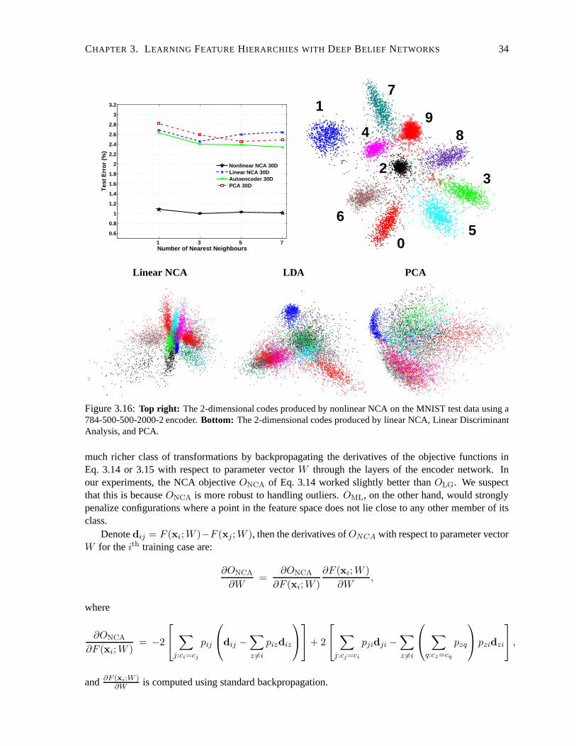
CHAPTER 3. LEARNING FEATURE HIERARCHIES WITH DEEP BELIEF NETWORKS 34
1 3 5 7
0.6
0.8
1
1.2
1.4
1.6
1.8
2
2.2
2.4
2.6
2.8
3
3.2
Number of Nearest Neighbours
Tes
t Err
or (
%)
Nonlinear NCA 30DLinear NCA 30DAutoencoder 30DPCA 30D
1
23
4
56
7
89
0
Linear NCA LDA PCA
Figure 3.16:Top right: The 2-dimensional codes produced by nonlinear NCA on the MNIST test data using a784-500-500-2000-2 encoder.Bottom: The 2-dimensional codes produced by linear NCA, Linear DiscriminantAnalysis, and PCA.
much richer class of transformations by backpropagating the derivatives of the objective functions inEq. 3.14 or 3.15 with respect to parameter vectorW through the layers of the encoder network. Inour experiments, the NCA objectiveONCA of Eq. 3.14 worked slightly better thanOLG. We suspectthat this is becauseONCA is more robust to handling outliers.OML, on the other hand, would stronglypenalize configurations where a point in the feature space does not lie close to any other member of itsclass.
Denotedij = F (xi;W )−F (xj ;W ), then the derivatives ofONCA with respect to parameter vectorW for theith training case are:
∂ONCA
∂W=
∂ONCA
∂F (xi;W )
∂F (xi;W )
∂W,
where
∂ONCA
∂F (xi;W )= −2
∑
j:ci=cj
pij
dij −
∑
z 6=i
pizdiz
+ 2
∑
j:cj=ci
pjidji −∑
z 6=i
∑
q:cz=cq
pzq
pzidzi
,
and ∂F (xi;W )∂W
is computed using standard backpropagation.
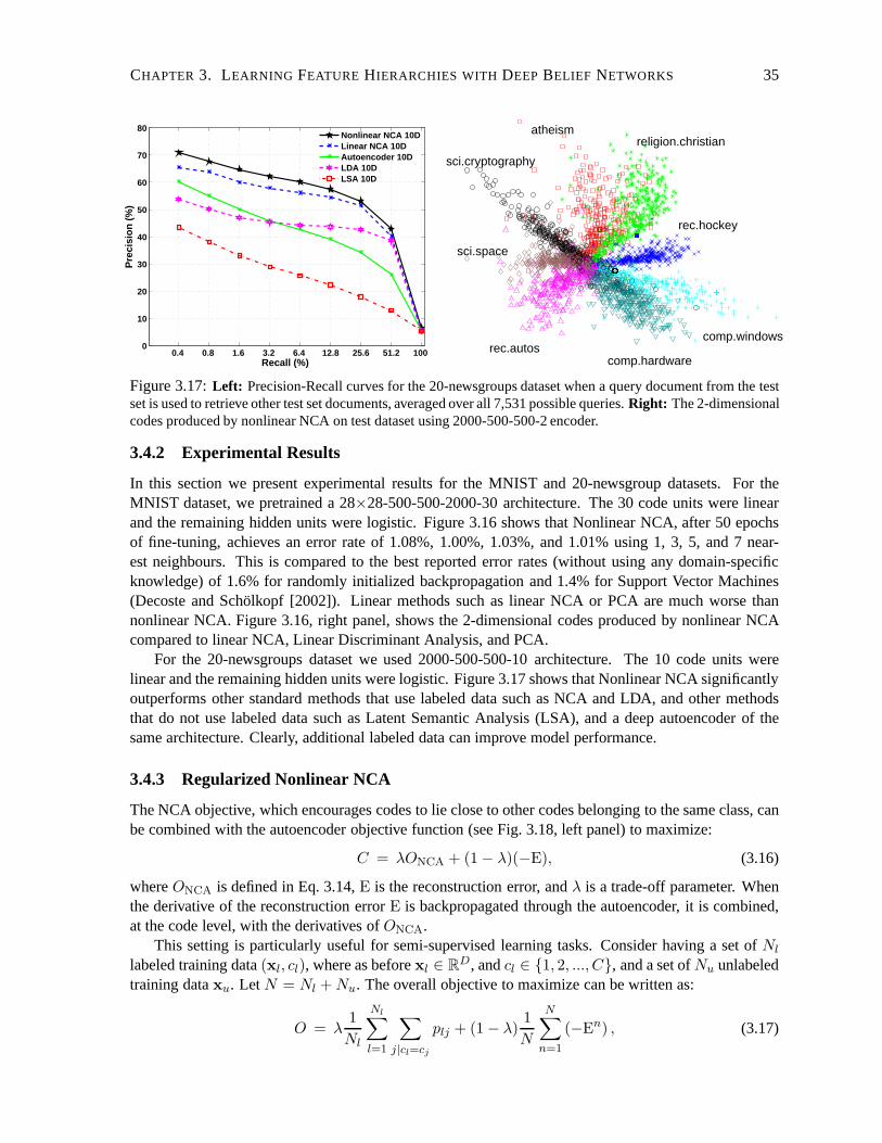
CHAPTER 3. LEARNING FEATURE HIERARCHIES WITH DEEP BELIEF NETWORKS 35
0.4 0.8 1.6 3.2 6.4 12.8 25.6 51.2 100 0
10
20
30
40
50
60
70
80
Recall (%)
Pre
cisi
on (
%)
Nonlinear NCA 10DLinear NCA 10DAutoencoder 10DLDA 10DLSA 10D
atheism
comp.hardware
comp.windowsrec.autos
rec.hockey
sci.cryptography
sci.space
religion.christian
Figure 3.17:Left: Precision-Recall curves for the 20-newsgroups dataset when a query document from the testset is used to retrieve other test set documents, averaged over all 7,531 possible queries.Right: The 2-dimensionalcodes produced by nonlinear NCA on test dataset using 2000-500-500-2 encoder.
3.4.2 Experimental Results
In this section we present experimental results for the MNIST and 20-newsgroup datasets. For theMNIST dataset, we pretrained a 28×28-500-500-2000-30 architecture. The 30 code units were linearand the remaining hidden units were logistic. Figure 3.16 shows that Nonlinear NCA, after 50 epochsof fine-tuning, achieves an error rate of 1.08%, 1.00%, 1.03%, and 1.01% using 1, 3, 5, and 7 near-est neighbours. This is compared to the best reported error rates (without using any domain-specificknowledge) of 1.6% for randomly initialized backpropagation and 1.4% for Support Vector Machines(Decoste and Scholkopf [2002]). Linear methods such as linear NCA or PCA are much worse thannonlinear NCA. Figure 3.16, right panel, shows the 2-dimensional codes produced by nonlinear NCAcompared to linear NCA, Linear Discriminant Analysis, and PCA.
For the 20-newsgroups dataset we used 2000-500-500-10 architecture. The 10 code units werelinear and the remaining hidden units were logistic. Figure3.17 shows that Nonlinear NCA significantlyoutperforms other standard methods that use labeled data such as NCA and LDA, and other methodsthat do not use labeled data such as Latent Semantic Analysis(LSA), and a deep autoencoder of thesame architecture. Clearly, additional labeled data can improve model performance.
3.4.3 Regularized Nonlinear NCA
The NCA objective, which encourages codes to lie close to other codes belonging to the same class, canbe combined with the autoencoder objective function (see Fig. 3.18, left panel) to maximize:
C = λONCA + (1− λ)(−E), (3.16)
whereONCA is defined in Eq. 3.14,E is the reconstruction error, andλ is a trade-off parameter. Whenthe derivative of the reconstruction errorE is backpropagated through the autoencoder, it is combined,at the code level, with the derivatives ofONCA.
This setting is particularly useful for semi-supervised learning tasks. Consider having a set ofNl
labeled training data(xl, cl), where as beforexl ∈ RD, andcl ∈ 1, 2, ..., C, and a set ofNu unlabeled
training dataxu. Let N = Nl + Nu. The overall objective to maximize can be written as:
O = λ1
Nl
Nl∑
l=1
∑
j|cl=cj
plj + (1− λ)1
N
N∑
n=1
(−En) , (3.17)

CHAPTER 3. LEARNING FEATURE HIERARCHIES WITH DEEP BELIEF NETWORKS 36
1 3 5 7 8
9
10
11
12
13
14
15
16
17
18
19
20
21
Number of Nearest Neighbours
Tes
t Err
or (
%)
Regularized NCA ( λ=0.99)Nonlinear NCA 30D ( λ=1)Linear NCA 30DAutoencoder 30D ( λ=0)KNN in pixel space
1 3 5 7 2.5
3
3.5
4
4.5
5
5.5
6
6.5
7
7.5
8
Number of Nearest Neighbours
Tes
t Err
or (
%)
Regularized NCA ( λ=0.99)Nonlinear NCA 30D ( λ=1)Linear NCA 30DAutoencoder 30D ( λ=0)KNN in pixel space
1 3 5 7 2
2.5
3
3.5
4
4.5
5
5.5
6
Number of Nearest Neighbours
Tes
t Err
or (
%)
Regularized NCA ( λ=0.999)Nonlinear NCA 30D ( λ=1)Linear NCA 30DAutoencoder 30D ( λ=0)KNN in pixel space
1% labels 5% labels 10% labels
Figure 3.18:KNN on the MNIST test set when only a small fraction of class labels is available. Linear NCAand KNN in pixel space do not take advantage of the unlabeled data.
whereEn is the reconstruction error for the input data vectorxn. For the MNIST dataset we use thecross-entropy error:
Ep = −∑
i
xni log xn
i −∑
i
(1− xni ) log(1− xn
i ), (3.18)
wherexni ∈ [0, 1] is the intensity of pixeli for the training examplen, and xn
i is the intensity of itsreconstruction.
When the number of labeled examples is small, regularized nonlinear NCA performs better thannonlinear NCA (λ = 1), which uses the unlabeled data for pretraining but ignoresit during the fine-tuning. It also performs better than an autoencoder (λ = 0), which ignores the labeled set. To testthe effect of the regularization when most of the data is unlabeled, we randomly sampled 1%, 5% and10% of the handwritten digits in each class and treated them as labeled data. The remaining digits weretreated as unlabeled data. Figure 3.18 reveals that regularized nonlinear NCA (λ = 0.99) outperformsboth nonlinear NCA (λ = 1) and an autoencoder (λ = 0). The parameterλ was selected using cross-validation from among the values0.5, 0.9, 0.99, 0.999. Even when the entire training set is labeled,regularized NCA still performs slightly better. In Chapter5 we will show that other deep models canoutperform regularized nonlinear NCA, even when the numberof labeled examples is small.
Splitting codes into class-relevant and class-irrelevantparts
To allow accurate reconstruction of a digit image, the code must contain information about aspects ofthe image such as its orientation, slant, size and stroke thickness that are not relevant to its classifica-tion. These irrelevant aspects necessarily contribute to the Euclidean distance between codes and harmclassification. To reduce this unwanted effect, we used 50-dimensional codes but only used the first30 dimensions in the NCA objective function. The remaining 20 dimensions were free to code all theaspects of an image that do not affect its class label but are important for its reconstruction.
Figure 3.18, right panel, shows how the reconstruction is affected by changing the activity level ofa single code unit. Changing a unit among the first 30 changes the class, while changing a unit amongthe last 20 does not. Withλ = 0.99 the split codes achieve an error rate of 1.00% 0.97% 0.98% 0.97%using 1, 3, 5, and 7 nearest neighbours. We also computed the 3NN error rate on the test set using onlythe last 20 code units. It was 4.3%, clearly indicating that the class-relevant information is concentratedin the first 30 units.
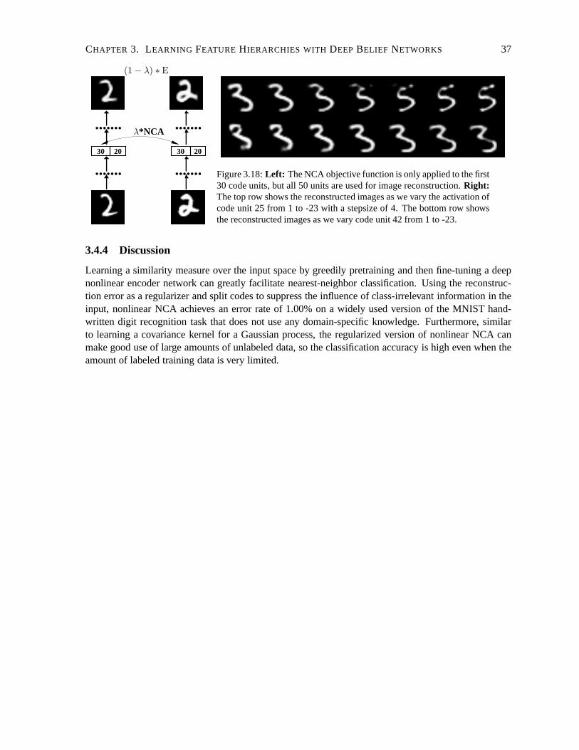
CHAPTER 3. LEARNING FEATURE HIERARCHIES WITH DEEP BELIEF NETWORKS 37
30 20 30 20
.......
.......
.......
.......λ*NCA
(1− λ) ∗ E
Figure 3.18:Left: The NCA objective function is only applied to the first30 code units, but all 50 units are used for image reconstruction. Right:The top row shows the reconstructed images as we vary the activation ofcode unit 25 from 1 to -23 with a stepsize of 4. The bottom row showsthe reconstructed images as we vary code unit 42 from 1 to -23.
3.4.4 Discussion
Learning a similarity measure over the input space by greedily pretraining and then fine-tuning a deepnonlinear encoder network can greatly facilitate nearest-neighbor classification. Using the reconstruc-tion error as a regularizer and split codes to suppress the influence of class-irrelevant information in theinput, nonlinear NCA achieves an error rate of 1.00% on a widely used version of the MNIST hand-written digit recognition task that does not use any domain-specific knowledge. Furthermore, similarto learning a covariance kernel for a Gaussian process, the regularized version of nonlinear NCA canmake good use of large amounts of unlabeled data, so the classification accuracy is high even when theamount of labeled training data is very limited.
Chapter 4
Evaluating Deep Belief Networks asDensity Models
Deep Belief Networks are generative models that contain many layers of hidden variables. Efficientgreedy algorithms for learning and approximate inference have allowed these models to be appliedsuccessfully in many application domains, as we discussed in chapter 3. The main building block of aDBN is a bipartite undirected graphical model called a Restricted Boltzmann Machine (RBM). Due tothe presence of the partition function exact maximum likelihood learning in RBM’s is intractable, andmodel selection and complexity control are difficult. In this chapter we show that a Monte Carlo basedmethod, Annealed Importance Sampling (AIS), can be used to efficiently estimate the partition functionof an RBM. We further show how an AIS estimator, along with approximate inference, can be used toestimate a lower bound on the log-probability that a DBN model with multiple hidden layers assigns tothe test data. This allows us to directly assess generalization performance of Deep Belief Networks asdensity models.
4.1 Introduction
Deep Belief Networks (DBN’s), reviewed in chapter 2, are probabilistic generative models that containseveral layers of latent variables. The greedy learning algorithm for DBN’s proceeds by learning astack of undirected graphical models, called Restricted Boltzmann Machines (RBM’s). A key feature ofRBM’s is that inference in these models is easy. An unfortunate limitation is that the probability of dataunder the model is known only up to a computationally intractable normalizing constant – the partitionfunction. A good estimate of the partition function would allow us to assess generalization performanceof RBM’s and DBN’s as density models. Indeed, assessing the generalization performance plays animportant role in model selection and complexity control. For many specific tasks, such as informationretrieval or object recognition, performance of RBM’s and DBN’s can be directly evaluated (Nair andHinton [2009], Bengio et al. [2007], Salakhutdinov and Hinton [2009b]). More broadly, however, themodel’s generalization capability can be evaluated by computing the probability that the model assignsto the previously unseen input vectors, which is independent of any specific application.
There has been extensive research on obtaining deterministic approximations (Yedidia et al. [2005])or deterministic upper bounds (Wainwright et al. [2005], Globerson and Jaakkola [2007]) on the log-partition function of arbitrary discrete Markov random fields (MRF’s). These variational methods relycritically on an ability to approximate the entropy of the undirected graphical model. However, fordensely connected MRF’s, such as RBM’s, these methods are unlikely to perform well (Salakhutdinov[2008]). There have also been many developments in the use ofMonte Carlo methods for estimating
38
CHAPTER 4. EVALUATING DEEP BELIEF NETWORKS ASDENSITY MODELS 39
the partition function, including Annealed Importance Sampling (AIS) (Neal [2001]), Nested Sampling(Skilling [2004]), and many others (see e.g. Neal [1993]). In this chapter we show how one such method,AIS, by taking advantage of the bipartite structure of an RBM, can be used to efficiently estimate itspartition function. We further show that this estimator, along with approximate inference, can be used toestimate a lower bound on the log-probability that a DBN model with multiple hidden layers assigns totraining or test data. This result will allow us to assess theperformance of DBN’s as generative modelsand to compare them to other probabilistic models, such as plain mixture models.
4.2 Estimating Partition Functions
Suppose we have two distributions defined on some spaceX with probability density functionsPA(x) =P ∗
A(x)/ZA andPB(x) = P ∗B(x)/ZB , whereP ∗(·) denotes the unnormalized probability density. Let
ΩA andΩB be the support sets ofPA andPB respectively. One way of estimating the ratio of normal-izing constants is to use a simple importance sampling (SIS)method. We use the following identity,assuming thatΩB ⊆ ΩA, i.e. PA(v) 6= 0 wheneverPB(v) 6= 0:
ZB
ZA
=
∫P ∗
B(x)dx
ZA
=
∫P ∗
B(x)
P ∗A(x)
PA(x)dx = EPA
[P ∗
B(x)
P ∗A(x)
].
Assuming we can draw independent samples fromPA, an unbiased estimate of the ratio of partitionfunctions can be obtained by using a simple Monte Carlo approximation:
ZB
ZA≈ 1
M
M∑
i=1
P ∗B(x(i))
P ∗A(x(i))
≡ 1
M
M∑
i=1
w(i) = rSIS, (4.1)
wherex(i) ∼ PA. If we choosePA(x) to be a tractable distribution for which we can computeZA
analytically, we obtain an unbiased estimate of the partition functionZB. However, ifPA andPB arenot close enough, the estimatorrSIS will be very poor. In high-dimensional spaces, the varianceof anestimatorrSIS will be very large, or possibly infinite (see MacKay [2003], chapter 29), unlessPA is anear-perfect approximation toPB .
4.2.1 Annealed Importance Sampling (AIS)
Suppose that we can define a sequence of intermediate probability distributions: P0, ..., PK , with P0 =PA andPK = PB , which satisfy the following conditions:
C1 Pk(x) 6= 0 wheneverPk+1(x) 6= 0.
C2 We must be able to easily evaluate the unnormalized probability P ∗k (x), ∀x ∈ X , k = 0, ...,K.
C3 For eachk = 1, ...,K−1, we must be able to draw a samplex′ givenx using a Markov chaintransition operatorTk(x
′←x) that leavesPk(x) invariant:
∫Tk(x
′←x)Pk(x)dx = Pk(x′). (4.2)
C4 We must be able to draw (preferably independent) samples from PA.

CHAPTER 4. EVALUATING DEEP BELIEF NETWORKS ASDENSITY MODELS 40
Algorithm 3 Annealed Importance Sampling (AIS) run.1: Selectβk with 0 = β0 < β1 < ... < βK = 1.2: Samplex1 from PA = P0.3: for k = 1 : K − 1 do4: Samplexk+1 givenxk usingTk(xk+1←xk).5: end for6: SetwAIS =
∏K
k=1P ∗
k (xk)/P ∗
k−1(xk).
The transition operatorsTk(x′←x) represent the probability or probability density of transitioning from
statex to x′. Constructing a suitable sequence of intermediate probability distributions will depend onthe problem. One general way to define this sequence is to set:
Pk(x) ∝ P ∗A(x)1−βkP ∗
B(x)βk , (4.3)
with 0 = β0 < β1 < ... < βK = 1 chosen by the user.A single run of the AIS procedure is summarized in Algorithm 3. Note that there is no need to
compute the normalizing constants of any intermediate distributions. After performingM runs of AIS,the importance weightsw(i)
AIS can be substituted into Eq. 4.1 to obtain an estimate of the ratio of partitionfunctions:
ZB
ZA
≈ 1
M
M∑
i=1
w(i)AIS = rAIS. (4.4)
It is shown in (Neal [2001, 2005]) that for sufficiently largenumber of intermediate distributionsK,the variance ofrAIS will be proportional to1/MK. ProvidedK is kept large, the total amount ofcomputation can be split in any way between the number of intermediate distributionsK and the numberof annealing runsM without adversely affecting the accuracy of the estimator.If samples drawn frompA are independent, the AIS runs can be used to obtain the variance of the estimaterAIS:
Var(rAIS) =1
MVar(w
(i)AIS
)≈ s2
M= σ2, (4.5)
wheres2 is estimated simply from the sample variance of the importance weights.The intuition behind AIS is the following. Consider the following identity:
ZK
Z0=Z1
Z0
Z2
Z1...ZK
ZK−1. (4.6)
Provided the two intermediate distributionsPk andPk+1 are close enough, a simple importance samplercan be used to estimate each ratioZk+1/Zk:
Zk+1
Zk
≈ 1
M
M∑
i=1
P ∗k+1(x
(i))
P ∗k (x(i))
, where x(i) ∼ Pk.
These ratios can then be used to estimateZK
Z0=∏K−1
k=0Zk+1
Zk. The problem with this approach is that,
except forP0, we typically cannot easily draw exact samples from intermediate distributionsPk. Wecould resort to Markov chain methods, but then it is hard to determine when the Markov chain hasconverged to the desired distribution.
A remarkable fact shown by Neal [2001], Jarzynski [1997] is that the estimate ofZK/Z0 will be ex-actly unbiased if each ratioZk+1/Zk is estimated usingM = 1, and a new sample is obtained by using

CHAPTER 4. EVALUATING DEEP BELIEF NETWORKS ASDENSITY MODELS 41
Markov chain starting at the previous sample. The proof of this fact relies on the observation that the AISprocedure is just a simple importance sampling defined on theextended state spaceX=(x1,x2, ...,xK).Indeed, AIS starts by first sampling from distributionP0(x) and then applying a series of transition op-eratorsT1, T2, . . . , TK−1 that “move” the sample through the intermediate distributionsPk(x) towardsthe target distributionPK(x). The probability of the resultant state sequenceX is given by:
Q(X) = P0(x1)
K−1∏
k=1
Tk(xk+1←xk). (4.7)
We can viewQ(X) as a proposal distribution for the target distributionP(X) on the extended spaceX.This target distribution is defined by the reverse AIS procedure:
P(X) = PK(xK)K−1∏
k=1
Tk(xk←xk+1), (4.8)
whereTk are the reverse transition operators:
Tk(x′←x) = Tk(x←x′)
Pk(x′)
Pk(x). (4.9)
If Tk is reversible thenTk is the same asTk. Due to invariance ofPk with respect toTk (Eq. 4.2), thereverse transition operators are valid transition probabilities, which ensures that the marginal distributionoverxK in Eq. 4.8 is the correct distribution of interestPK(xK). Denoting the unnormalized proposaland target distributions asQ∗(X) = Z0Q(X) andP∗(X) = ZKP(X), the importance weight can befound using Eq. 4.1:
w =P∗(X)
Q∗(X)=ZKP(X)
Z0Q(X)=ZKPK(xK)
∏K−1i=1 Tk(xk←xk+1)
Z0P0(x1)∏K−1
k=1 Tk(xk+1←xk)
=P ∗
K(xK)
P ∗0 (x1)
K−1∏
k=1
P ∗k (xk)
P ∗k (xk+1)
=
K∏
k=1
P ∗k (xk)
P ∗k−1(xk)
, (4.10)
which are the weights provided by the AIS algorithm. Observethat the Markov transition operators donot necessarily need to be ergodic. In particular, if we wereto choose dumb transition operators thatdo nothing,Tk(x
′ ← x) = δ(x′ − x) for all k, we recover the original simple importance samplingprocedure.
4.2.2 Ratios of Partition Functions of two RBM’s
As discussed in section 2.1, a Restricted Boltzmann Machinehas a two-layer architecture in which thevisible, binary stochastic unitsv ∈ 0, 1D are connected to hidden binary stochastic unitsh ∈ 0, 1F .The energy of the statev,h is:
E(v,h; θ) = −v⊤Wh−b⊤v−a⊤h
= −D∑
i=1
F∑
j=1
Wijvihj−D∑
i=1
bivi−F∑
j=1
ajhj, (4.11)
CHAPTER 4. EVALUATING DEEP BELIEF NETWORKS ASDENSITY MODELS 42
whereθ = W,b,a are the model parameters. The probability that the model assigns to a visiblevectorv is:
P (v; θ) =1
Z(θ)
∑
h
exp (−E(v,h; θ))
=1
Z(θ)exp(b⊤v)
F∏
j=1
(1 + exp
(aj +
D∑
i=1
Wijvi
)). (4.12)
Suppose we have two RBM’s with parameter valuesθA = W A,bA,aA andθB = W B ,bB ,aBthat define probability distributionsPA and PB over V ∈ 0, 1D . Each RBM can have a differentnumber of hidden unitshA ∈ 0, 1FA andhB ∈ 0, 1FB . Using Eq. 4.12, we could define genericAIS intermediate distributions on the state spacex = v, as defined in Eq. 4.3. However, samplingfrom these intermediate distributions would be slower thansampling from an RBM. Instead, we canmake use of the bipartite structure of an RBM by introducing the following sequence of distributionsfor k = 0, ...,K:
Pk(v) =P ∗
k (v)
Zk
=1
Zk
∑
h
exp (−Ek(v,h)), (4.13)
where the energy function is given by:
Ek(v,h) = (1− βk)E(v,hA; θA) + βkE(v,hB ; θB), (4.14)
with 0 = β0 < β1 < ... < βK = 1 and h = hA,hB. For i = 0, we haveβ0 = 0 and soP0 = PA. Similarly, for i = K, we havePK = PB . For the intermediate values ofk, we will havesome interpolation betweenPA andPB .
Let us now define a Markov chain transition operatorTk(v′←v) that leavesPk(v) invariant. Using
Eqs. 4.13, 4.14, it is straightforward to derive a Gibbs sampler. The conditional distributions are givenby logistic functions:
p(hAj = 1|v) = g
((1− βk)
(∑
i
W Aij vi + aA
j
)), (4.15)
p(hBj = 1|v) = g
(βk
(∑
i
W Bij vi + aB
j
)), (4.16)
p(v′i = 1|h) = g
(1− βk)
∑
j
W Aij hA
j + bAi
+ βk(
∑
j
W Bij hB
j + bBi )
, (4.17)
whereg(x) = 1/(1 + exp(−x)). Givenv, Eqs. 4.15, 4.16 are used to stochastically activate hiddenunitshA andhB . Eq. 4.17 is then used to draw a new samplev′ as shown in Fig. 4.1, left panel. Due tothe special structure of RBM’s, the cost of summing outh is linear in the number of hidden units. Wecan therefore easily evaluate:
P ∗k (v) =
∑
hA,hB
e(1−βk)E(v,hA;θA)+βkE(v,hB ;θB)
= e(1−βk)P
i bAi vi
FA∏
j=1
(1 + e(1−βk)(
P
i W Aij vi+aA
j )) × eβk
P
i bBi vi
FB∏
j=1
(1 + eβk(
P
i W Bij vi+aB
j )) .

CHAPTER 4. EVALUATING DEEP BELIEF NETWORKS ASDENSITY MODELS 43
v v′
(1− βk)WA βkW
B
βkWB (1− βk)W
A
hA hB
Model A Model B
P(v|h1;W1)
P(h1,h2;W2)
Figure 4.1:Left: The Gibbs transition operatorTk(v′←v) leavesPk(v) invariant when estimating the ratio ofpartition functionsZB/ZA. Right: Two-hidden-layer Deep Belief Network as a generative model.
We will assume that the parameter values of each RBM satisfy|θ| < ∞, in which caseP (v) > 0for all v ∈ V. This will ensure that condition C1 of the AIS procedure is always satisfied. We havealready shown that conditions C2 and C3 are satisfied. For condition C4, we can run a Gibbs sampler(Eqs. 2.7, 2.8) to generate samples fromPA. These sample points will not be independent, but the AISestimator will still converge to the correct value, provided our Markov chain is ergodic (Neal [2001]).However, assessing the accuracy of this estimator can be difficult, as it depends on both the variance ofthe importance weights and on autocorrelations in the Gibbssampler.
4.2.3 Estimating Partition Functions of RBM’s
In the previous section we showed that we can use AIS to obtainan estimate ofZB/ZA. Consider anRBM with parameter vectorθA = 0,bA,aA, i.e. an RBM with a zero weight matrix. From Eq. 4.12,we know:
ZA =∏
j
(1 + eaj
)∏
i
(1 + ebi
). (4.18)
Moreover,
PA(v) =∏
i
pA(vi) =∏
i
1/(1 + e−bi),
so we can draw exact independent samples from this “base-rate” RBM. AIS in this case allows us toobtain anunbiasedestimate of the partition functionZB. This approach closely resembles simulated an-nealing (Kirkpatrick et al. [1983], Bertsimas and Tsitsiklis [1993]), since the intermediate distributionsof Eq. 4.13 take form:
Pk(v) =exp
((1−βk)
(vTbA
))
Zk
∑
hB
exp(−βkE
(v,hB ; θB
)).
We gradually changeβk (the inverse temperature) from 0 to 1, annealing from a simple “base-rate”model to the final complex model.
4.3 Estimating Lower Bounds for DBN’s
Let us consider the Deep Belief Network with two layers of hidden features shown in Fig. 4.1, rightpanel. The model’s joint distribution is:
P (v,h1,h2) = P (v|h1)P (h2,h1), (4.19)

CHAPTER 4. EVALUATING DEEP BELIEF NETWORKS ASDENSITY MODELS 44
whereP (v|h1) is the sigmoid belief network (Eq. 2.8), andP (h1,h2) is the joint distribution definedby the second layer RBM. Note thatP (v|h1) is normalized.
By explicitly summing outh2, we can easily evaluate an unnormalized probabilityP ∗(v,h1) =ZP (v,h1). Using the approximating factorial distributionQ of Eq. 2.19, which we get as a byproductof the greedy learning procedure, and the variational lowerbound of Eq. 2.17, we obtain:
log∑
h1
P (v,h1) ≥∑
h1
Q(h1|v) log P ∗(v,h1)− logZ +H(Q(h1|v)) = B(v). (4.20)
The entropy termH(·) can be computed analytically, sinceQ is factorial. The partition functionZ isestimated by running AIS on the top-level RBM. And the expectation term can be estimated by a simpleMonte Carlo approximation:
∑
h1
Q(h1|v) log P ∗(v,h1) ≈ 1
M
M∑
i=1
log P ∗(v,h1(i)), (4.21)
whereh1(i) ∼ Q(h1|v). The variance of this Monte Carlo estimator will be proportional to 1/Mprovided the variance oflog P ∗(v,h1(i)) is finite. In general, we will be interested in calculating thelower bound averaged over the test set containingNt samples:
1
Nt
Nt∑
n=1
B(vn) ≈ 1
Nt
Nt∑
n=1
[1
M
M∑
i=1
log p∗(vn,h1(i)) +H(Q(h1|vn))
]− log Z
= rB − log Z = rBound. (4.22)
In this case the variance of the estimator induced by the Monte Carlo approximation will asymptoticallyscale as1/(NtM). We will show in the experimental results section that the value of M can be smallprovidedNt is large. The error of the overall estimatorrBound in Eq. 4.22 will be mostly dominated bythe error in the estimate oflogZ.
Estimating this lower bound for Deep Belief Networks with more layers is now straightforward.Consider a DBN withL hidden layers. The model’s joint distribution and its approximate factorialposterior distributionQ are given by (see section 2.2):
P (v,h1, ...,hL) = P (v|h1)...P (hL−2|hL−1)P (hL−1,hL),
Q(h1, ...,hL|v) = Q(h1|v)Q(h2|v)...Q(hL|v).
The estimate of the lower bound can now be obtained by using Eqs. 4.20, 4.22. Note that most of thecomputation resources will be spent on estimating the partition functionZ of the top level RBM.
4.4 Experimental Results
In our experiments we used the MNIST digit dataset, which contains 60,000 training and 10,000 testimages of ten handwritten digits (0 to 9), with 28×28 pixels. The dataset was binarized: each pixelvalue was stochastically set to 1 in proportion to its pixel intensity. Samples from the training set areshown in Fig. 4.2, middle left panel. Annealed importance sampling requires us to specifyβk that definea sequence of intermediate distributions. In all of our experiments this sequence was chosen by quicklyrunning a few preliminary experiments and picking the spacing ofβk so as to minimize the variance ofthe final importance weights. For the base-rate model the biases of the hidden unitsaA were set to zero(see Eq. 4.18) and the biases of the visible unitsbA were set by maximum likelihood, then smoothed toensure thatP (v) > 0, ∀ v ∈ V. In all experiments we obtained unbiased estimates ofZ and its standarddeviationσ using Eqs. 4.4, 4.5. We also use natural logarithms, providing values in nats. Details of theMatlab code, used in experiments, can be found in Appendix A.

CHAPTER 4. EVALUATING DEEP BELIEF NETWORKS ASDENSITY MODELS 45
Base-rateβ = 0 β = 0.5 β = 0.95 β = 1.0
The course of an AIS run for model CD25(500)
Training samples MoB (100) CD1(500) CD3(500)
CD25(500) DBN-CD1(500)-CD1(2000) DBN-CD3(500)-CD3(2000) DBN-CD25(500)-CD25(2000)
Figure 4.2:Top row: displays the course of 16 AIS runs for CD25(500) model by starting from a simple base-rate model and annealing to the final complex model.Middle row: First two panels show random samples fromthe training set and a mixture of Bernoullis model with 100 components. The last 2 panels display random samplesgenerated from two RBM’s.Bottom row: Random samples generated from an RBM and three DBN models.
4.4.1 Estimating partition functions of RBM’s
In our first experiment we trained three RBM’s on the MNIST digits. The first two RBM’s had 25 hiddenunits and were learned using Contrastive Divergence (subsection 2.1) withT=1 andT=3 respectively.We call these models CD1(25) and CD3(25). The third RBM had 20hidden units and was learned usingCD with T=1. For all three models we can calculate the exact value of the partition function simplyby summing out the 784 visible units for each configuration ofthe hiddens. For all three models weused 500βk spaced uniformly from 0 to 0.5, 4,000βk spaced uniformly from 0.5 to 0.9, and 10,000βk
spaced uniformly from 0.9 to 1.0, with a total of 14,500 intermediate distributions.Table 4.1 shows that AIS can rather quickly provide an accurate estimate of the partition function.
For all three models, using only 10 AIS runs, we were able to obtain good estimates of partition functionsin just 20 seconds on a Pentium Xeon 3.00GHz machine. For model CD1(25), however, the variance ofthe estimator was high, even with 100 AIS runs. Figure 4.3, top row, further reveals that as the numberof annealing runs is increased, AIS can almost exactly recover the true value of the partition functionacross all three models.
We also directly estimated the ratio of normalizing constants of two RBM’s that have differentnumbers of hidden units: CD1(20) and CD1(25). This estimator could be used to do complexitycontrol. In detail, using 100 AIS runs with uniform spacing of 10,000βk, we obtainedlog rAIS =
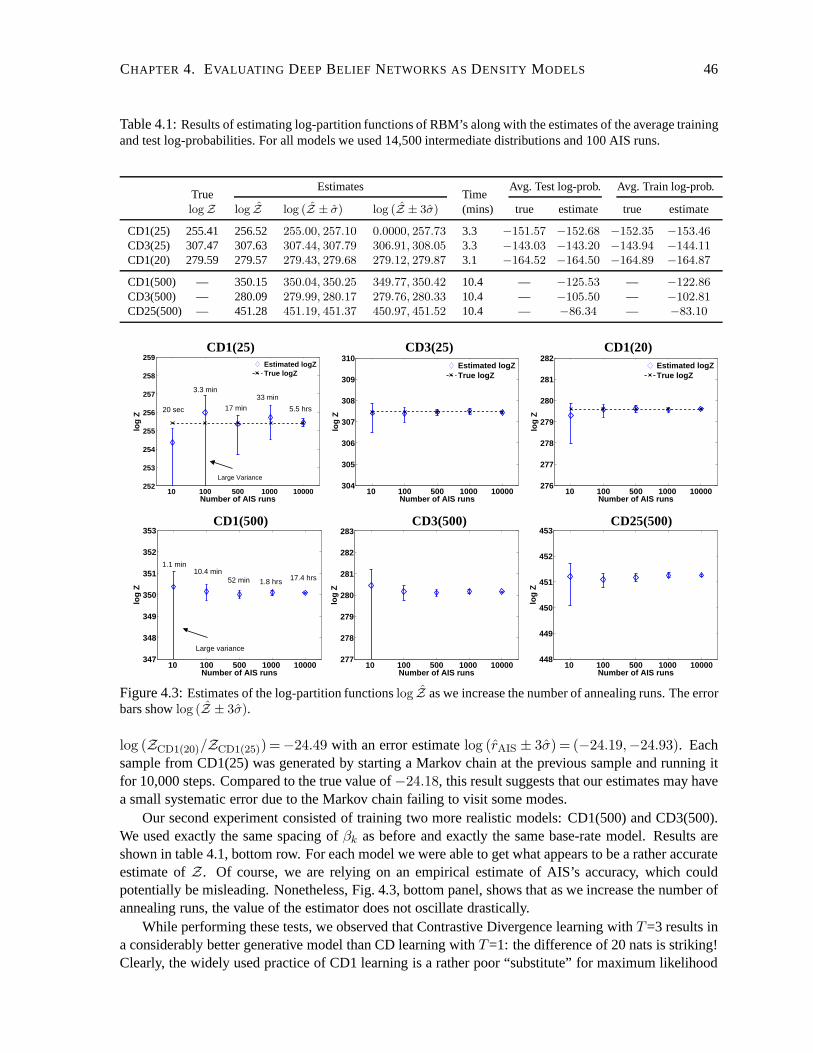
CHAPTER 4. EVALUATING DEEP BELIEF NETWORKS ASDENSITY MODELS 46
Table 4.1:Results of estimating log-partition functions of RBM’s along with the estimates of the average trainingand test log-probabilities. For all models we used 14,500 intermediate distributions and 100 AIS runs.
TrueEstimates
TimeAvg. Test log-prob. Avg. Train log-prob.
logZ log Z log (Z ± σ) log (Z ± 3σ) (mins) true estimate true estimate
CD1(25) 255.41 256.52 255.00, 257.10 0.0000, 257.73 3.3 −151.57 −152.68 −152.35 −153.46CD3(25) 307.47 307.63 307.44, 307.79 306.91, 308.05 3.3 −143.03 −143.20 −143.94 −144.11CD1(20) 279.59 279.57 279.43, 279.68 279.12, 279.87 3.1 −164.52 −164.50 −164.89 −164.87
CD1(500) — 350.15 350.04, 350.25 349.77, 350.42 10.4 — −125.53 — −122.86CD3(500) — 280.09 279.99, 280.17 279.76, 280.33 10.4 — −105.50 — −102.81CD25(500) — 451.28 451.19, 451.37 450.97, 451.52 10.4 — −86.34 — −83.10
10 100 500 1000 10000252
253
254
255
256
257
258
259
Number of AIS runs
log
Z
Large Variance
20 sec
3.3 min
17 min
33 min
5.5 hrs
Estimated logZTrue logZ
10 100 500 1000 10000304
305
306
307
308
309
310
Number of AIS runs
log
Z
Estimated logZTrue logZ
10 100 500 1000 10000276
277
278
279
280
281
282
Number of AIS runs
log
Z
Estimated logZTrue logZ
CD1(25) CD3(25) CD1(20)
10 100 500 1000 10000347
348
349
350
351
352
353
Number of AIS runs
log
Z
Large variance
1.1 min10.4 min
52 min 1.8 hrs 17.4 hrs
10 100 500 1000 10000277
278
279
280
281
282
283
Number of AIS runs
log
Z
10 100 500 1000 10000448
449
450
451
452
453
Number of AIS runs
log
ZCD1(500) CD3(500) CD25(500)
Figure 4.3:Estimates of the log-partition functionslog Z as we increase the number of annealing runs. The errorbars showlog (Z ± 3σ).
log (ZCD1(20)/ZCD1(25)) =−24.49 with an error estimatelog (rAIS ± 3σ) = (−24.19,−24.93). Eachsample from CD1(25) was generated by starting a Markov chainat the previous sample and running itfor 10,000 steps. Compared to the true value of−24.18, this result suggests that our estimates may havea small systematic error due to the Markov chain failing to visit some modes.
Our second experiment consisted of training two more realistic models: CD1(500) and CD3(500).We used exactly the same spacing ofβk as before and exactly the same base-rate model. Results areshown in table 4.1, bottom row. For each model we were able to get what appears to be a rather accurateestimate ofZ. Of course, we are relying on an empirical estimate of AIS’s accuracy, which couldpotentially be misleading. Nonetheless, Fig. 4.3, bottom panel, shows that as we increase the number ofannealing runs, the value of the estimator does not oscillate drastically.
While performing these tests, we observed that ContrastiveDivergence learning withT=3 results ina considerably better generative model than CD learning with T=1: the difference of 20 nats is striking!Clearly, the widely used practice of CD1 learning is a ratherpoor “substitute” for maximum likelihood

CHAPTER 4. EVALUATING DEEP BELIEF NETWORKS ASDENSITY MODELS 47
Table 4.2:Results of estimating lower boundsrBound (Eq. 4.22) on the average training and test log-probabilitiesfor DBN’s. On average, the total error of the estimator is about± 2 nats.
Estimates Avg. bound on log-prob.
log Z log (Z ± 3σ) Test ± 3std Train ± 3std.
DBN-CD1(500)-CD1(2000) 277.33 275.90, 277.90 −100.64 ±0.77 −97.67 ±0.30DBN-CD3(500)-CD3(2000) 229.92 229.01, 230.23 −98.29 ±0.75 −94.86 ±0.29DBN-CD25(500)-CD25(2000) 466.70 465.86, 467.35 −86.22 ±0.67 −82.47 ±0.25
learning. Inspired by this result, we trained a model by starting with T=1, and gradually increasingTto 25 during the course of CD learning, as suggested by Carreira-Perpinan and Hinton [2005]. We callthis model CD25(500). Training this model was computationally much more demanding. However, theestimate of the average test log-probability for this modelwas about−86, which is 39 and 19 nats betterthan the CD1(500) and CD3(500) models respectively. Figure4.2 shows samples generated from allthree models by randomly initializing binary states of the visible units and running the Gibbs samplerfor 100,000 steps. Certainly, samples generated by CD25(500) look much more like the real handwrittendigits, than either CD1(500) or CD3(500).
Using 10,000βk and 100 annealing runs, we also obtained an estimate of the log ratio of twopartition functionsrAIS = logZCD25(500)/ZCD3(500) = 169.96. The estimates of the individual log-
partition functions werelog ZCD25(500) = 451.28 and log ZCD3(500) = 280.09, in which case the logratio is451.28−280.09 = 171.19. This is in agreement (to within three standard deviations)with thedirect estimate of the ratio,rAIS =169.96.
For a simple comparison we also trained several mixture of Bernoullis models (see Fig. 4.2, middleleft panel) with 10, 100, and 500 components. The corresponding average test log-probabilities were−168.95, −142.63, and−137.64. The data generated from the mixture model with 100 componentslooks better than either CD1(500) or CD3(500), although ourquantitative results reveal this is due tooverfitting. Restricted Boltzmann Machines give much higher density to test data.
4.4.2 Estimating lower bounds for DBN’s
We trained three Deep Belief Networks with two hidden layers. The first model, which we call DBN-CD1(500)-CD1(2000), was greedily learned by freezing the parameter vector of the CD1(500) modeland fitting the2nd layer RBM with 2000 hidden units using CD withT=1. Similarly, the other twomodels, DBN-CD3(500)-CD3(2000) and DBN-CD25(500)-CD25(2000), added 2000 hidden units ontop of CD3(500) and CD25(500), and were learned using CD withT=3 andT=25 respectively. Trainingthe DBN’s took roughly three times longer than the RBM’s.
Table 4.2 shows the results. We used 15,000 intermediate distributions and 500 annealing runs toestimate the partition function of the2nd layer RBM, which took 2.3 hours. We further usedM=5samples from the approximating distributionQ(h|v) to do a simple Monte Carlo approximation ofEq. 4.21. SettingM=100 did not make much difference. Table 4.2 also reports theempirical error in theestimate of the lower boundrBound. From Eq. 4.22, we have Var(rBound) = Var(rB)+Var(log Z), bothof which are shown in table 4.2. Note that the two-hidden-layer Deep Belief Networks, DBN-CD1(500)-CD1(2000) and DBN-CD3(500)-CD3(2000), significantly outperform their single layer counterparts:CD1(500) and CD3(500). Adding a second layer for those two models improves model performance byat least 25 and 7 nats. Figure 4.2 also shows the dramatic difference between samples generated by thesingle layer RBM’s and corresponding two-hidden-layer DBN’s.

CHAPTER 4. EVALUATING DEEP BELIEF NETWORKS ASDENSITY MODELS 48
Table 4.3:Results of estimating lower bounds on the average test log-probabilities for DBN’s. On average, thetotal error of the estimator is about± 2 nats.
No 2nd 2ndlayer
1st layer layer CD1(500) CD3(500) CD25(500) CD1(2000) CD3(2000) CD25(2000)
DBN-CD1(500)- -125.53 -101.40 -97.54 -89.52 -100.64 -94.44 -87.13DBN-CD3(500)- -105.50 -100.27 -95.21 -88.38 -101.62 -98.29 -88.92DBN-CD25(500)- -86.34 -101.55 -98.38 -86.90 -98.57 -96.97 -86.22
DBN-CD1(2000)- -122.84 -134.81 -119.45 -90.50 -116.44 -100.08 -92.53DBN-CD3(2000)- -100.92 -112.81 -107.49 -89.48 -106.67 -98.73 -91.25DBN-CD25(2000)- -86.26 -121.83 -112.64 -89.96 -102.24 -97.87 -88.29
Surprisingly, the greedy learning of DBN’s does not appear to suffer severely from overfitting. Forsingle layer models, the difference between the estimates of training and test log-probabilities was about3 nats. For DBN’s, the corresponding difference in the estimates of the lower bounds was about 4 nats,even though adding a second layer introduced over twice as many (or one million) new parameters.
The result of our experiments for DBN-CD25(500)-CD25(2000), however, was very different. Forthis model, on the test data we obtainedrBound =−86.22. This is comparable to the estimate of−86.34for the average test log-probability of the CD25(500) model. Clearly, we cannot confidently assert thatthe DBN is a better generative model compared to the carefully trained single layer RBM. This peculiarresult also supports previous claims that if the first level RBM already models data well, adding extralayers will not help (LeRoux and Bengio [2008], Hinton et al.[2006]).
To estimate how loose the variational bound is, we randomly sampled 50 test cases, 5 of each class,and ran AIS for each test case to estimate the true test log probability. Computationally, this is equivalentto estimating 50 additional partition functions. Our estimate of the variational bound was 87.05 per testcase. The estimate of the true test log probability was 85.20, showing that the bound is actually rathertight.
To further examine the effect that CD learning has on pretraining a stack of RBM’s, we trainedadditional 36 models. Table 4.3 shows results of estimatingthe lower bound on the average test log-probabilities. These results support our two previous observations. First, when training a lower-levelRBM with CD1 or CD3, adding an extra layer generally improvesmodel performance. Second, when alower-level RBM already models data well, adding an extra layer does not help. Performance of modelsDBN-CD1(2000)-CD1(500), DBN-CD3(2000)-CD3(500), and DBN-CD25(2000)-CD25(500) furtherreveals that decreasing the number of hidden units per layercan actually hurt model performance.
As an additional test, instead of randomly initializing parameters of the2nd layer RBM, we initial-ized it by using the same parameters as the1st layer RBM but with hidden and visible units switched,so that the2nd and3rd layers contained 500 and 784 hidden units. This initialization ensures that thedistribution over the visible unitsv defined by the two-hidden-layer DBN isexactly the sameas thedistribution overv defined by the1st layer RBM (see section 2.2). Therefore, after learning parame-ters of the2nd layer RBM, the lower bound on the training data log-likelihood should improve. Aftercarefully training the second level RBM, our estimate of thelower bound on the test log-probabilitywas−85.97. Once again, we cannot confidently claim that adding an extralayer in this case yieldsbetter generalization.
4.5 DiscussionAs we discussed in chapter 2, under some strong assumptions,each additional layer of a DBN increasesa lower bound on the log-probability of thetraining data, provided the number of hidden units per layer
CHAPTER 4. EVALUATING DEEP BELIEF NETWORKS ASDENSITY MODELS 49
does not decrease. However, assessing generalization performance of these generative models is quitedifficult, since computing the exact probability of a test vector requires enumeration over an exponentialnumber of terms. In this chapter we developed an Annealed Importance Sampling procedure that takesadvantage of the bipartite structure of the RBM. This can provide a good estimate of the partitionfunction in a reasonable amount of computer time. Furthermore, we showed that this estimator, alongwith approximate inference, can be used to obtain an estimate of the lower bound on the log-probabilityof thetestdata. This allowed us to obtain some quantitative evaluation of the generalization performanceof these deep hierarchical models.
There are some disadvantages to using AIS. There is a need to specify theβk that define a sequenceof intermediate distributions. The number and the spacing of βk will be problem dependent and willaffect the variance of the estimator. We also have to rely on the empirical estimate of AIS accuracy,which could potentially be very misleading (Neal [2001, 2005]). Even though AIS provides an unbiasedestimator ofZ, it may often give large underestimates and occasionally give even larger overestimates.So in practice, it is more likely to underestimate the true value of the partition function, which will resultin an overestimate of the log-probability. But these drawbacks should not result in disfavoring the useof AIS for RBM’s and DBN’s: it is much better to have a slightlyunreliable estimate than no estimate atall, or an extremely indirect estimate, such as discriminative performance (Hinton et al. [2006], Bengioet al. [2007]). We also find Annealed Importance Sampling andother stochastic methods attractivebecause they can just as easily be applied to undirected graphical models that generalize RBM’s andDBN’s to exponential family distributions. This will allowfuture application to models of real-valueddata, such as image patches (Osindero and Hinton [2008]), orcount data (Gehler et al. [2006]).
Another alternative would be to employ deterministic approximations (Yedidia et al. [2005]) or de-terministic upper bounds (Wainwright et al. [2005]) on the log-partition function. However, for denselyconnected MRF’s, we would not expect these methods to work well. My own findings (Salakhutdi-nov [2008]) show that these methods provide quite inaccurate estimates of (or very loose upper boundson) the partition function, even for small RBM’s whentrained on real datathat has many modes withsimilar probabilities.

Chapter 5
Deep Boltzmann Machines
In this chapter we present a new learning algorithm for a different type of hierarchical probabilisticmodel: a Deep Boltzmann Machine (DBM). Unlike Deep Belief Networks, a DBM is a type of Markovrandom field, or undirected graphical model, where all connections between layers are undirected. DeepBoltzmann Machines are interesting for several reasons. First, like Deep Belief Networks, DBM’s havethe potential of learning internal representations that become increasingly complex at higher layers,which is a promising way of solving object and speech recognition problems. High-level representationscan be built from a large supply of unlabeled sensory inputs and the very limited labeled data canthen be used to only slightly fine-tune the model for a specifictask at hand. Second, unlike DeepBelief Networks and many other models with deep architectures (Ranzato et al. [2007], Vincent et al.[2008], Serre et al. [2007]), the approximate inference procedure, in addition to a bottom-up pass, canincorporate top-down feedback, allowing Deep Boltzmann Machines to better propagate uncertaintyabout ambiguous inputs. This is perhaps the most important distinguishing characteristic of this model.Finally, in the presence of enormous amounts of sensory data, the entire model can be trained online,processing one example at a time.
5.1 Introduction
The original learning algorithm for Boltzmann machines, introduced by Hinton and Sejnowski [1983],used randomly initialized Markov chains in order to performapproximate inference to estimate themodel’s expected sufficient statistics. This learning procedure, however, was too slow to be practical.There have been many attempts in developing efficient learning and inference algorithms for Boltzmannmachines (see Welling and Hinton [2002], Welling and Teh [2003], Zhu and Liu [2002] and referencestherein), but none of them have proven to be useful for large-scale problems in machine learning.
In this chapter we present an efficient learning procedure for fully general Boltzmann machines. Ap-proximate inference can be performed using variational approaches, such as mean-field. Learning canthen be carried out by applying a stochastic approximation procedure that uses Markov chain MonteCarlo (MCMC) to approximate a model’s expected sufficient statistics. The MCMC based approxi-mation procedure provides nice asymptotic convergence guarantees and belongs to the general classof approximation algorithms of Robbins–Monro type (Robbins and Monro [1951], Younes [1989]).This unusual combination of variational methods and MCMC isessential for creating a fast learningalgorithm for general Boltzmann machines, or, more generally, undirected graphical models in the ex-ponential family (Wainwright and Jordan [2003]). If the connections between hidden units are restrictedin such a way that the hidden units form multiple layers, it ispossible to modify the greedy learningalgorithm for Restricted Boltzmann Machines so that they can be used to initialize the parameters of a
50
CHAPTER 5. DEEP BOLTZMANN MACHINES 51
Deep Boltzmann Machine before applying our new learning procedure. Finally, we present results onthe MNIST and NORB datasets showing that Boltzmann machineslearn good generative models andperform well on handwritten digit and visual object recognition tasks.
5.2 Boltzmann Machines (BM’s)
A Boltzmann machine is a network of symmetrically coupled stochastic binary units. It contains a setof visible unitsv ∈ 0, 1D , and a set of hidden unitsh ∈ 0, 1F (see Fig. 5.1, left panel), thatmodel complicated, higher-order correlations between thevisible units. The energy of the statev,his defined as:
E(v,h; θ) = −1
2v⊤Lv− 1
2h⊤Jh− v⊤Wh, (5.1)
whereθ = W,L, J are the model parameters1: W , L, J represent visible-to-hidden, visible-to-visible, and hidden-to-hidden symmetric interaction terms. The diagonal elements ofL andJ are set to0. The probability that the model assigns to a visible vectorv is:
P (v; θ) =P ∗(v; θ)
Z(θ)=
1
Z(θ)
∑
h
exp (−E(v,h; θ)), (5.2)
Z(θ) =∑
v
∑
h
exp (−E(v,h; θ)), (5.3)
whereP ∗ denotes unnormalized probability, andZ(θ) is the partition function. Theconditionaldistri-butions over hidden and visible units are given by:
p(hj = 1|v,h−j) = g
∑
i
Wijvi +∑
m6=j
Jjmhj
, (5.4)
p(vi = 1|h,v−i) = g
∑
j
Wijhj +∑
k 6=i
Likvj
, (5.5)
whereg(x) = 1/(1 + exp(−x)) is the logistic function andx−i denotes a vectorx but withxi omitted.The parameter updates, originally derived by Hinton and Sejnowski [1983], that are needed to performgradient ascent in the log-likelihood can be obtained from Eq. 5.2:
∆W = α(
EPdata[vh⊤]− EPmodel
[vh⊤])
,
∆L = α(
EPdata[vv⊤]− EPmodel
[vv⊤])
,
∆J = α(
EPdata[hh⊤]− EPmodel
[hh⊤])
,
whereα is a learning rate. EPdata[·] denotes an expectation with respect to the completed data dis-
tribution Pdata(h,v; θ) = P (h|v; θ)Pdata(v), with Pdata(v) = 1N
∑n δ(v − vn) representing the
empirical distribution, and EPmodel[·] is an expectation with respect to the distribution defined bythe
model (Eq. 5.2). We will sometimes refer to EPdata[·] as thedata-dependent expectation, and EPmodel
[·]as themodel’s expectation.
1We have omitted the bias terms for clarity of presentation

CHAPTER 5. DEEP BOLTZMANN MACHINES 52
L
J
W
General Boltzmann MachineRestricted Boltzmann Machine
Figure 5.1:Left: A general Boltzmann machine. The top layer represents a vector of stochastic binary “hidden”features and the bottom layer represents a vector of stochastic binary “visible” variables.Right: A RestrictedBoltzmann Machine with no hidden-to-hidden and no visible-to-visible connections.
Exact maximum likelihood learning in this model is intractable. The exact computation of the data-dependent expectation takes time that is exponential in thenumber of hidden units, whereas the exactcomputation of the model’s expectation takes time that is exponential in the number of hidden andvisible units. Hinton and Sejnowski [1983] proposed an algorithm that uses Gibbs sampling (Gemanand Geman [1984]) to approximate both expectations. For each iteration of learning, a separate Markovchain is run for every training data vector to approximate EPdata
[·], and an additional chain is run toapproximate EPmodel
[·]. The main problem with this learning algorithm is the time required to approachthe stationary distribution, especially when estimating the model’s expectations, since the Gibbs chainmay need to explore a highly multimodal energy landscape. This is typical when modeling real-worlddistributions, such as datasets of images, in which almost all of the possible images have extremely lowprobability, but there are many very different images that occur with quite similar probabilities.
Setting bothJ=0 andL=0 recovers the Restricted Boltzmann Machine (RBM) model (see Fig. 5.1,right panel). Although exact maximum likelihood learning in RBM’s is still intractable, learning canbe carried out efficiently using Contrastive Divergence (CD) (Hinton [2002]). It was further observed(Welling and Hinton [2002], Hinton [2002]) that for Contrastive Divergence to perform well, it is im-portant to obtain exact samples from the conditional distribution P (h|v; θ), which is intractable whenlearning full Boltzmann machines.
5.2.1 A Stochastic Approximation Procedure for Estimatingthe Model’s Expectations
Instead of using CD learning, it is possible to make use of a stochastic approximation procedure (SAP)that uses MCMC methods to stochastically approximate the model’s expectations (Younes [1989, 2000],Neal [1992], Yuille [2004], Tieleman [2008]). SAP belongs to the general class of well-studied stochas-tic approximation algorithms of the Robbins–Monro type (Younes [1989], Robbins and Monro [1951]).To be more precise, let us consider the following canonical form of the exponential family associatedwith the sufficient statistics vectorΦ:
P (x; θ) =1
Z(θ)exp (θ⊤Φ(x)). (5.6)
The derivative of the log-likelihood for an observationx0 with respect to parameter vectorθ is:
∂ log P (x0; θ)
∂θ= Φ(x0)− EPmodel
[Φ(x)]. (5.7)
The idea behind learning parameter vectorθ using SAP is straightforward. Letθt andxt be the currentparameters and the state. Thenxt andθt are updated sequentially as follows:

CHAPTER 5. DEEP BOLTZMANN MACHINES 53
Algorithm 4 Stochastic Approximation Algorithm.
1: Randomly initializeθ0 andM sample particlesx0,1, ...., x0,M.2: for t = 0 : T (number of iterations)do3: for i = 1 : M (number of parallel Markov chains)do4: Samplext+1,i givenxt,i using transition operatorTθt(xt+1,i← xt,i).5: end for6: Update:θt+1 = θt + αt
[Φ(x0)− 1
M
∑Mm=1 Φ(xt+1,m)
].
7: Decreaseαt.8: end for
• Given xt, a new statext+1 is sampled from the transition operatorTθt(xt+1 ← xt) that leavesP (·; θt) invariant.
• A new parameterθt+1 is then obtained by replacing the intractable model’s expectation EPmodel[Φ(x)]
with Φ(xt)
In practice, we typically maintain a set ofM sample pointsXt = xt,1, ...., xt,M, which we will oftenrefer to as sample particles. In this case, the intractable model’s expectation is replaced by the sampleaverage1/M
∑Mm=1 Φ(xt+1,m). The procedure is summarized in Algorithm 4.
The proof of convergence of these algorithms relies on the following basic decomposition. First, thegradient of the log-likelihood function takes the form:
S(θ) =∂ log P (x; θ)
∂θ= Φ(x0)− EPmodel
[Φ(x)]. (5.8)
The parameter update rule then takes the following form:
θt+1 = θt + αt
[Φ(x0)−
1
M
M∑
m=1
Φ(xt+1,m)
](5.9)
= θt + αtS(θt) + αt
[EPmodel
[Φ(x)]− 1
M
M∑
m=1
Φ(xt+1,m)
]
= θt + αtS(θt) + αtǫt+1. (5.10)
The first term is the discretization of the ordinary differential equationθ = S(θ). The algorithm istherefore a perturbation of this discretization with the noise termǫ. The proof then proceeds by showingthat the noise term is not too large.
Precise sufficient conditions that ensure almost sure convergence to an asymptotically stable pointof θ = S(θ) are given in Younes [1989, 2000], Yuille [2004]. One necessary condition requires thelearning rate to decrease with time, so that
∑∞t=0 αt = ∞ and
∑∞t=0 α2
t < ∞. This condition can,for example. be satisfied simply by settingαt = 1/(t0 + t). Other conditions ensure that the speed ofconvergence of the Markov chain, governed by the transitionoperatorTθ, does not decrease too fast asθ tends to infinity, and that the noise termǫ in the update of Eq. 5.9 is bounded. Typically, in practice,the sequence|θt| is bounded, and the Markov chain, governed by the transitionkernelTθ, is ergodic.Together with the condition on the learning rate, this ensures almost sure convergence of SAP to anasymptotically stable point ofθ = S(θ).
The intuition behind why this procedure works is the following. As the learning rate becomessufficiently small compared with the mixing rate of the Markov chain, this “persistent” chain will always

CHAPTER 5. DEEP BOLTZMANN MACHINES 54
stay very close to the stationary distribution, even if it isonly run for a few MCMC steps per parameterupdate. Samples from the persistent chain will be highly correlated for successive parameter updates.However, if the learning rate is sufficiently small, the chain will mix before the parameters have changedenough to significantly alter the value of the estimator. This technique for learning Boltzmann machineswas used by Neal [1992]. When applied to learning RBM’s, Tieleman [2008] further shows that thisstochastic approximation algorithm, also termed Persistent Contrastive Divergence, performs quite wellcompared to Contrastive Divergence learning.
5.2.2 A Variational Approach to Estimating the Data-Dependent Expectations
In variational learning (Hinton and Zemel [1994], Neal and Hinton [1998], Jordan et al. [1999]), thetrue posterior distribution over latent variablesP (h|v; θ) for each training vectorv, is replaced byan approximate posteriorQ(h|v;µ) and the parameters are updated to maximize the variational lowerbound on the log-likelihood:
log P (v; θ) ≥∑
h
Q(h|v;µ) log P (v,h; θ) +H(Q)
= log P (v; θ)− KL [Q(h|v;µ)||P (h|v; θ)] , (5.11)
whereH(·) is the entropy functional. Variational learning has the nice property that in addition totrying to maximize the log-likelihood of the training data,it tries to find parameters that minimize theKullback-Leibler divergences between the approximating and true posteriors. Using a naive mean-field approach, we choose a fully factorized distribution inorder to approximate the true posterior:Q(h;µ) =
∏Fj=1 q(hi), with q(hi = 1) = µi andF is the number of hidden units. The lower bound on
the log-probability of the data takes the following form:
log P (v; θ) ≥ 1
2
∑
i,k
Likvivk +1
2
∑
j,m
Jjmµjµm +∑
i,j
Wijviµj − logZ(θ)
+∑
j
[µj log µj + (1− µj) log (1− µj)] .
The learning proceeds by first maximizing this lower bound with respect to the variational parametersµ for fixedθ, which results in the mean-field fixed-point equations:
µj ← g
∑
i
Wijvi +∑
m6=j
Jmjµm
. (5.12)
This is followed by applying SAP to update the model parameters θ. We emphasize that variational ap-proximations cannot be used for approximating the expectations with respect to the model distributionin the Boltzmann machine learning rule, as attempted in Galland [1991], because the minus sign wouldcause variational learning to adjust the parameters so as tomaximizethe divergence between the approx-imating and true distributions. If, however, a Markov chainis used to estimate the model’s expectations,variational learning can be applied for estimating the data-dependent expectations.
The choice of naive mean-field was deliberate. First, the convergence is usually fast, which greatlyfacilitates learning. Second, for applications such as theinterpretation of images or speech, we expectthe posterior over hidden statesgiven the datato have a single mode, so simple and fast variationalapproximations such as mean-field should be adequate. Indeed, making the true posterior unimodalby sacrificing some log-likelihood could be advantageous for a system that will use the posterior to

CHAPTER 5. DEEP BOLTZMANN MACHINES 55
Algorithm 5 Boltzmann Machine Learning Procedure.
1: Given: a training set ofN binary data vectorsvNn=1, andM , the number of samples.2: Randomly initialize parameter vectorθ0 andM samples:v0,1, h0,1, ..., v0,M , h0,M.3: for t = 0 to T (number of iterations)do
4: // Variational Inference:5: for each training examplevn, n = 1 to N do6: Randomly initializeµ and run mean-field updates until convergence:
µj ← g(∑
i Wijvi +∑
m6=j Jmjµm
).
7: Setµn = µ.8: end for
9: // Stochastic Approximation:10: for each samplem = 1 to M do11: Sample(vt+1,m, ht+1,m) given(vt,m, ht,m) by running a Gibbs sampler (Eqs. 5.4, 5.5).12: end for
13: // Parameter Update:
14: W t+1 = W t + αt
(1N
∑Nn=1 vn(µn)⊤ − 1
M
∑Mm=1 vt+1,m(ht+1,m)⊤
).
15: J t+1 = J t + αt
(1N
∑Nn=1 µn(µn)⊤ − 1
M
∑Mm=1 ht+1,m(ht+1,m)⊤
).
16: Lt+1 = Lt + αt
(1N
∑Nn=1 vn(vn)⊤ − 1
M
∑Mm=1 vt+1,m(vt+1,m)⊤
).
17: Decreaseαt.18: end for
control its actions. Having multiple alternative representations of the same sensory input increases thelikelihood, but makes it far more difficult to associate an appropriate action with that sensory input. Themean-field inference helps to eliminate this problem. During learning, if the posterior given a traininginput vector is multimodal, the mean-field inference will lock onto exactly one mode, and learningwill make that mode more probable. Our learning algorithm will therefore tend to find regions in theparameter space in which the true posterior is unimodal.
5.3 Deep Boltzmann Machines (DBM’s)
In general, we will rarely be interested in learning a complex, fully connected Boltzmann machine.Instead, we will focus on learning Deep Boltzmann Machines (see Fig. 5.2, right panel). Unlike DeepBelief Networks, a Deep Boltzmann Machine is a Markov randomfield, where all connections betweenlayers are undirected.
Consider a three-hidden-layer Boltzmann machine, as shownin Fig. 5.2, right panel, with no within-layer connections. The energy of the statev,h1,h2,h3 is defined as:
E(v,h1,h2,h3; θ) = −v⊤W 1h1 − h1⊤W 2h2,−h2⊤W 3h3, (5.13)
whereθ = W 1,W 2,W 3 are the model parameters, representing visible-to-hiddenand hidden-to-

CHAPTER 5. DEEP BOLTZMANN MACHINES 56
h3
h2
h1
v
W3
W2
W1
Deep Belief Network Deep Boltzmann Machine
Figure 5.2:Left: Deep Belief Network, with the top two layers forming an undirected graph and the remaininglayers form a belief net with directed, top-down connectionsRight: Deep Boltzmann machine, with both visible-to-hidden and hidden-to-hidden connections but with no within-layer connections.
hidden symmetric interaction terms. The probability that the model assigns to a visible vectorv is:
P (v; θ) =1
Z(θ)
∑
h1,h2,h3
exp (−E(v,h1,h2,h3; θ)). (5.14)
The conditional distributions over the visible and the three sets of hidden units are given by logisticfunctions:
p(h1j = 1|v,h2) = g
(∑
i
W 1ijvi +
∑
m
W 2jmh2
m
), (5.15)
p(h2m = 1|h1,h3) = g
∑
j
W 2jmh1
j +∑
l
W 3mlh
3l
, (5.16)
p(h3l = 1|h2) = g
(∑
m
W 3mlh
2m
), (5.17)
p(vi = 1|h1) = g
∑
j
W 1ijh
1j
. (5.18)
For approximate maximum likelihood learning, we could still apply the learning procedure for generalBoltzmann machines described above, but it would be rather slow, particularly when the hidden unitsform layers that become increasingly remote from the visible units. There is, however, a fast way toinitialize the model parameters to good values, which we describe in the next section.
5.3.1 Greedy Layerwise Pretraining of DBM’s
In chapter 2 we reviewed a greedy, layer-by-layer unsupervised learning algorithm that consists of learn-ing a stack of RBM’s one layer at a time. After greedy learning, the whole stack can be viewed as asingle probabilistic model called a Deep Belief Network. Surprisingly, this composite model isnot aDeep Boltzmann Machine. The top two layers form a RestrictedBoltzmann Machine, but the lowerlayers form adirectedsigmoid belief network (see Fig. 5.2, left panel).

CHAPTER 5. DEEP BOLTZMANN MACHINES 57
RBM
RBM
RBM
v v
W1 W1
h1
h1
h2
h2
h3 h3
2W2
W3 W3
W1
W2
W3
Pretraining
Deep Boltzmann Machine
Figure 5.3: Pretraining a DBM with three hidden layers consists of learning a stack of RBM’s that are thencomposed to create a Deep Boltzmann Machine. The first and last RBM’s in the stack need to be modified bycopying the visible or hidden units.
After learning the first RBM in the stack, the generative model can be written as:
P (v; θ) =∑
h1
P (h1;W 1)P (v|h1;W 1), (5.19)
whereP (h1;W 1) =∑
vP (h1,v;W 1) is an implicit prior overh1. The second RBM in the stack
attempts to learn a better model forP (h1;W 2) by maximizing the variational lower bound (see Eq. 2.17)with respect toW 2. If initialized correctly, the2nd layer RBMP (h1;W 2) will become a better modelof the aggregated posterior overh1, which is simply the mixture of factorial posteriors for allthe trainingcases:1
N
∑n P (h1|vn;W 1) (see section 2.2). Since the2nd layer RBM replacesP (h1;W 1) by a better
model, inferringP (h1;W 1,W 2) would be possible by taking a geometric average of the two modelsof h1, which could be approximated by using1/2W 1 bottom-up and1/2W 2 top-down. But usingW 1
bottom-up andW 2 top-down would effectively double the total input into the hidden unitsh1, whichmay cause saturation.
To initialize model parameters of a DBM, we propose greedy, layer-by-layer pretraining heuristic bylearning a stack of RBM’s, but with a small change that is introduced to eliminate the doubling effect.For the lower-level RBM, to compensate for the lack of top-down input intoh1, we double the inputand tie the visible-to-hidden weights, as shown in Fig. 5.3,left panel. In this modified RBM with tiedparameters, the conditional distributions over the hiddenand visible states are defined as:
p(h1j = 1|v) = g
(2∑
i
W 1ijvi
), (5.20)
p(vi = 1|h1) = g
∑
j
W 1ijh
1j
. (5.21)

CHAPTER 5. DEEP BOLTZMANN MACHINES 58
Algorithm 6 Greedy Pretraining Algorithm for a Deep Boltzmann Machine with L-layers.
1: Make two copies of the visible vector and tie the visible-to-hidden weightsW 1. Fit W 1 of the1st layer RBM to data.
2: FreezeW 1 that defines the1st layer of features, and use sampleshl from P (h1|v, 2W 1) (Eq. 5.20)as the data for training the next layer RBM with weight vector2W 2.
3: FreezeW 2 that defines the2nd layer of features and use the samplesh2 from P (h2|h1, 2W 2) asthe data for training the3rd layer RBM with weight vector2W 3.
4: Proceed recursively for the next layersL− 1.5: When learning the top-level RBM, double the number of hiddenunits and tie the visible-to-hidden
weightsW L.6: Use the weightsW 1,W 2, ....,WL to compose a Deep Boltzmann Machine.
Contrastive Divergence learning works well and the modifiedRBM is good at reconstructing its trainingdata. Conversely, for the top-level RBM, to compensate for the lack of bottom-up input intoh2, wedouble the number of hidden units. The conditional distributions for this model take the form:
p(h2m = 1|h3) = g
(∑
l
W 3mlh
3(a)
l +∑
l
W 3mlh
3(b)
l
)(5.22)
p(h3l = 1|h2) = g
(∑
m
W 3mlh
2m
). (5.23)
For the intermediate RBM we simply double the weights. The conditional distributions take the form:
p(h1j = 1|h2) = g
(2∑
m
W 2jmh2
m
)(5.24)
p(h2m = 1|h1) = g
2∑
j
W 2jmh1
j
. (5.25)
When these three modules are composed to form a single system, the total input coming into thefirst and second hidden layers is halved, which leads to the following conditional distribution overh1
andh2:
p(h1j = 1|v,h2) = g
(∑
i
W 1ijvi +
∑
m
W 2jmh2
m
), (5.26)
p(h2m = 1|h1,h3) = g
∑
j
W 2jmh1
j +∑
l
W 3mlh
3l
. (5.27)
The conditional distributions overv andh3 remain the same as defined by Eqs. 5.21, 5.23.Observe that the conditional distributions defined by the composed model are exactly the same con-
ditional distributions defined by the DBM (Eqs. 5.15, 5.16, 5.17, 5.18). Therefore greedily pretrainingthe stack of modified RBM’s leads to an undirected model with symmetric weights – a Deep BoltzmannMachine. We note that the modification only needs to be used for the first and the last RBM’s in thestack. For all the intermediate RBM’s we simply halve their weights in both directions when composingthem to form a Deep Boltzmann Machine.

CHAPTER 5. DEEP BOLTZMANN MACHINES 59
Greedily pretraining the weights of a DBM in this way serves two purposes. First, it initializes theweights to reasonable values. Second, it ensures that thereis a fast way of performing approximateinference by a single upward pass through the stack of modified RBM’s. Given an input vector, eachlayer of hidden units can be activated in a single deterministic bottom-up pass by doubling the bottom-up input to compensate for the lack of top-down feedback, except for the very top layer, which does nothave a top-down input. This fast approximate inference is used to initialize the mean-field, which thenconverges much faster than the mean-field with random initialization.
5.3.2 Evaluating DBM’s
In chapter 4 we showed that a Monte Carlo based method, Annealed Importance Sampling (AIS), canbe used to efficiently estimate the partition function of an RBM. In this section we show how AIS canbe used to estimate the partition functions of Deep Boltzmann Machines. Together with variationalinference this will allow us obtain good estimates of the lower bound on the log-probability of the trainand test data.
Using the special layer-by-layer structure of DBM’s, we canderive an efficient AIS scheme forestimating the model’s partition function. Let us considera three-hidden-layer Boltzmann machine (seeFig. 5.3, right panel) whose energy is defined as:
E(v,h1,h2,h3; θ) = −v⊤W 1h1 − h1⊤W 2h2 − h2⊤W 3h3. (5.28)
By explicitly summing out the1st and the3rd layer hidden unitsh1,h3, we can easily evaluatean unnormalized probabilityP ∗(v,h2; θ). We can therefore run AIS on a much smaller state spacex = v,h2 with h1 andh3 analytically summed out. The sequence of intermediate distributions,parameterized byβ, is defined as follows:
Pk(v,h2; θ) =∑
h1,h3
Pk(v,h1,h2,h3; θ)
=1
Zk
∏
j
(1 + eβk(
P
i viW1ij+
P
m h2mW 2
jm))∏
l
(1 + eβk(
P
m h2mW 3
ml))
.
We gradually changeβk (the inverse temperature) from 0 to 1, annealing from a simple “uniform” modelto the final complex model. Using Eqs. 5.15, 5.16, 5.17, 5.18,it is straightforward to derive a Gibbstransition operator that leavesPk(v,h2; θ) invariant:
p(h1j = 1|v,h2) = g
(βk
(∑
i
W 1ijvi +
∑
m
W 2jmh2
m
)), (5.29)
p(h2m = 1|h1,h3) = g
βk
∑
j
W 2jmh1
j +∑
l
W 3mlh
3l
, (5.30)
p(h3l = 1|h2) = g
(βk
∑
m
W 3mlh
2m
), (5.31)
p(vi = 1|h1) = g
βk
∑
j
W 1ijh
1j
. (5.32)
Once we obtain an estimate of the global partition functionZ, we can estimate, for a given test case
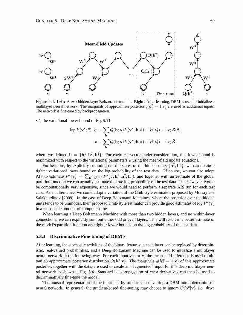
CHAPTER 5. DEEP BOLTZMANN MACHINES 60
v
h1
h2
W1
W2
...
v v v v
2W1 W1
W2 W2
Q(h1)
Q(h2)
y y
Fine-tune Q(h2)
W2 W1
W2
W3Mean-Field Updates
Figure 5.4:Left: A two-hidden-layer Boltzmann machine.Right: After learning, DBM is used to initialize amultilayer neural network. The marginals of approximate posteriorq(h2
j = 1|v) are used as additional inputs.The network is fine-tuned by backpropagation.
v∗, the variational lower bound of Eq. 5.11:
log P (v∗; θ) ≥ −∑
h
Q(h;µ)E(v∗,h; θ) +H(Q)− logZ(θ)
≈ −∑
h
Q(h;µ)E(v∗,h; θ) +H(Q)− log Z,
where we definedh = h1,h2,h3. For each test vector under consideration, this lower boundismaximized with respect to the variational parametersµ using the mean-field update equations.
Furthermore, by explicitly summing out the states of the hidden unitsh2,h3, we can obtain atighter variational lower bound on the log-probability of the test data. Of course, we can also adoptAIS to estimateP ∗(v) =
∑h1,h2,h3 P ∗(v,h1,h2,h3), and together with an estimate of the global
partition function we can actually estimate the true log-probability of the test data. This however, wouldbe computationally very expensive, since we would need to perform a separate AIS run for each testcase. As an alternative, we could adopt a variation of the Chib-style estimator, proposed by Murray andSalakhutdinov [2009]. In the case of Deep Boltzmann Machines, where the posterior over the hiddenunits tends to be unimodal, their proposed Chib-style estimator can provide good estimates oflog P ∗(v)in a reasonable amount of computer time.
When learning a Deep Boltzmann Machine with more than two hidden layers, and no within-layerconnections, we can explicitly sum out either odd or even layers. This will result in a better estimate ofthe model’s partition function and tighter lower bounds on the log-probability of the test data.
5.3.3 Discriminative Fine-tuning of DBM’s
After learning, the stochastic activities of the binary features in each layer can be replaced by determin-istic, real-valued probabilities, and a Deep Boltzmann Machine can be used to initialize a multilayerneural network in the following way. For each input vectorv, the mean-field inference is used to ob-tain an approximate posterior distributionQ(h2|v). The marginalsq(h2
j = 1|v) of this approximateposterior, together with the data, are used to create an “augmented” input for this deep multilayer neu-ral network as shown in Fig. 5.4. Standard backpropagation of error derivatives can then be used todiscriminatively fine-tune the model.
The unusual representation of the input is a by-product of converting a DBM into a deterministicneural network. In general, the gradient-based fine-tuningmay choose to ignoreQ(h2|v), i.e. drive

CHAPTER 5. DEEP BOLTZMANN MACHINES 61
the1st layer connectionsW 2 to zero, which will result in a standard neural network. Conversely, thenetwork may choose to ignore the input by driving the1st layer weightsW 1 to zero, and make itspredictions based on only the approximate posterior. However, the network typically makes use of theentire augmented input for making predictions.
5.4 Experimental Results
In our experiments we used the MNIST and NORB datasets. To speed-up learning, we subdivideddatasets into mini-batches, each containing 100 cases, andupdated the weights after each mini-batch.The number of sample particles, used for approximating the model’s expected sufficient statistics, wasalso set to 100. For the stochastic approximation algorithm, we always used 5 Gibbs updates. Eachmodel was trained using 300,000 weight updates. The initiallearning rate was set 0.005 and was de-creased as 10/(2000+t). For discriminative fine-tuning of DBM’s we used the method of conjugategradients. Details of pretraining and fine-tuning, along with details of Matlab code that we used forlearning and fine-tuning Deep Boltzmann Machines, can be found in Appendix A.
MNIST
The MNIST digit dataset contains 60,000 training and 10,000test images of ten handwritten digits(0 to 9), with 28×28 pixels. In our first experiment we trained a fully connected “flat” BM on theMNIST dataset. The model had 500 hidden units and 784 visibleunits. To estimate the model’s partitionfunction we used 20,000βk spaced uniformly from 0 to 1. Results are shown in table 5.1. The lowerbound on the average test log-probability was−84.67 per test case, which is slightly better compared tothe lower bound of−85.97, achieved by a carefully trained two-hidden-layer Deep Belief Network (seesection 4.4).
In our second experiment, we trained two Deep Boltzmann Machines: one with two hidden layers(500 and 1000 hidden units), and the other with three hidden layers (500,500, and 1000 hidden units),as shown in Fig. 5.6. To estimate the model’s partition function, we also used 20,000 intermediatedistributions spaced uniformly from 0 to 1. Table 5.1 shows that the estimates of the lower bound onthe average test log-probability were−84.62 and−85.18 for the 2- and 3-layer Boltzmann machinesrespectively.
Observe that the two DBM’s that contain over 0.9 and 1.15 million parameters do not appear to suf-fer much from overfitting. The difference between the estimates of the training and test log-probabilitieswas about 1 nat. Figure 5.5 further shows samples generated from all three models by randomly initializ-ing all binary states and running the Gibbs sampler for 100,000 steps. Certainly, all samples look like thereal handwritten digits. We also emphasize that without greedy pretraining, we could not successfullylearn good DBM models of MNIST digits.
To estimate how loose the variational bound is, we randomly sampled 100 test cases, 10 of eachclass, and ran AIS to estimate the true test log-probability2 for the 2-layer Boltzmann machine. Theestimate of the variational bound was -83.35 per test case, whereas the estimate of the true test log-probability was -82.86. The difference of about 0.5 nats shows that the bound is rather tight.
Finally, after discriminative fine-tuning, the two-hidden-layer BM achieves an error rate of 0.95% onthe full MNIST test set. This is, to our knowledge, the best published result on the permutation-invariantversion of the MNIST task. The 3-layer BM gives a slightly worse error rate of 1.01%. The flat BM,on the other hand, gives considerably worse error rate of 1.27%. This is compared to 1.4% achievedby SVM’s (Decoste and Scholkopf [2002]), 1.6% achieved by randomly initialized backprop, 1.2%
2Note that computationally, this is equivalent to estimating 100 partition functions.

CHAPTER 5. DEEP BOLTZMANN MACHINES 62
Training samples Flat BM 2-layer BM 3-layer BM
Figure 5.5:Random samples from the training set, and samples generatedfrom three Boltzmann machines byrunning the Gibbs sampler for 100,000 steps. The images shown are theprobabilitiesof the binary visible unitsgiven the binary states of the hidden units
4000 units
4000 units
4000 units
Preprocessedtransformation
Stereo pair
Gaussian visible units (raw pixel data)
500 units
1000 units
500 units
500 units
1000 units
28 x 28pixelimage
28 x 28pixelimage
2-layer BM
3-layer BM 3-layer BM
Figure 5.6:Left: The architectures of two Deep Boltzmann Machines used in MNIST experiments.Right: Thearchitecture of Deep Boltzmann Machine used in NORB experiments.
achieved by the Deep Belief Network, described in (Hinton etal. [2006], Hinton and Salakhutdinov[2006]), and 0.97% obtained by using a combination of discriminative and generative fine-tuning on thesame DBN (Hinton [2007]).
To test discriminative performance of DBM’s when the numberof labeled examples is small, werandomly sampled 1%, 5%, and 10% of the handwritten digits ineach class and treated them as labeleddata. Table 5.2 shows that after discriminative fine-tuning, a two-hidden-layer BM achieves error rates of4.82%, 2.72%, and 2.46%. Deep Boltzmann Machines clearly outperform regularized nonlinear NCA,discussed in section 3.4, as well as linear NCA, an autoencoder, and K-nearest neighbours, particularlywhen the number of labeled examples is only 600.
NORB
Results on MNIST show that Deep Boltzmann Machines can significantly outperform many other mod-els on the well-studied but relatively simple task of handwritten digit recognition. In this section wepresent results on NORB, which is considerably more difficult dataset than MNIST. NORB (LeCunet al. [2004]) contains images of 50 different 3D toy objectswith 10 objects in each of five genericclasses: cars, trucks, planes, animals, and humans. Each object is captured from different viewpoints

CHAPTER 5. DEEP BOLTZMANN MACHINES 63
Table 5.1:Results of estimating partition functions of BM models, along with the estimates of lower bound onthe average training and test log-probabilities. For all BM’s we used 20,000 intermediate distributions. Resultswere averaged over 100 AIS runs.
Estimates Avg. log-prob.
log Z log (Z ± σ) Test Train
Flat BM 198.29 198.17, 198.40 −84.67 −84.352-layer BM 356.18 356.06, 356.29 −84.62 −83.613-layer BM 456.57 456.34, 456.75 −85.10 −84.49
Table 5.2:Classification error rates on MNIST test set when only a smallfraction of labeled data is available.
Two-Layer Regularized Linear Autoencoder KNNDBM Nonlinear NCA NCA
1% (600) 4.82% 8.81% 19.37% 9.62% 13.74%5% (3000) 2.72% 3.24% 7.23% 5.18% 7.19%10% (6000) 2.46% 2.58% 4.89% 4.46% 5.87%100% (60000) 0.95% 1.00% 2.45% 2.41% 3.09%
and under various lighting conditions. The training set contains 24,300 stereo image pairs of 25 objects,5 per class, while the test set contains 24,300 stereo pairs of the remaining, different 25 objects. Thegoal is to classify each previously unseen object into its generic class. From the training data, 4,300were set aside for validation.
Each image has 96×96 pixels with integer greyscale values in the range [0,255]. To speed-upexperiments, we reduced the dimensionality by using a foveal representation of each image in a stereopair. The central 64×64 portion of an image is kept at its original resolution. Theremaining 16 pixel-wide ring around it is compressed by replacing non-overlapping square blocks of pixels in the ring witha single scalar given by the average pixel-value of a block. We split the ring into four smaller ones:the outermost ring consists of 8×8 blocks, followed by a ring of 4×4 blocks, and finally two innermostrings of 2×2 blocks. The resulting dimensionality of each training vector, representing a stereo pair,was2 × 4488 = 8976. A random sample from the training data used in our experiments is shown inFig. 5.7, left panel3.
To model raw pixel data, we use an RBM with Gaussian visible and binary hidden units. GaussianRBM’s have been previously successfully applied for modeling greyscale images, such as images offaces (see subsection 3.2.1). However, learning an RBM withGaussian units can be slow, particularlywhen the input dimensionality is quite large. Here we followthe approach of Nair and Hinton [2009] byfirst learning a Gaussian RBM and then treating the the activities of its hidden layer as “preprocessed”data. Effectively, the learned low-level RBM acts as a preprocessor that converts greyscale pixels into abinary representation, which we then use for learning a DeepBoltzmann Machine.
The number of hidden units for the preprocessing RBM was set to 4000 and the model was trainedusing Contrastive Divergence learning for 500 epochs. We then trained a two-hidden-layer DBM witheach layer containing 4000 hidden units, as shown in Fig. 5.6, right panel. Note that the entire modelwas trained in a completely unsupervised way. After the subsequent discriminative fine-tuning, the“unrolled” DBM achieves a misclassification error rate of 10.8% on the full test set. This is compared
3We thank Vinod Nair for sharing his code for blurring and translating NORB images.
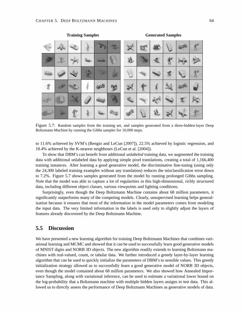
CHAPTER 5. DEEP BOLTZMANN MACHINES 64
Training Samples Generated Samples
Figure 5.7: Random samples from the training set, and samples generatedfrom a three-hidden-layer DeepBoltzmann Machine by running the Gibbs sampler for 10,000 steps.
to 11.6% achieved by SVM’s (Bengio and LeCun [2007]), 22.5% achieved by logistic regression, and18.4% achieved by the K-nearest neighbours (LeCun et al. [2004]).
To show that DBM’s can benefit from additionalunlabeledtraining data, we augmented the trainingdata with additional unlabeled data by applying simple pixel translations, creating a total of 1,166,400training instances. After learning a good generative model, the discriminative fine-tuning (using onlythe 24,300 labeled training examples without any translation) reduces the misclassification error downto 7.2%. Figure 5.7 shows samples generated from the model byrunning prolonged Gibbs sampling.Note that the model was able to capture a lot of regularities in this high-dimensional, richly structureddata, including different object classes, various viewpoints and lighting conditions.
Surprisingly, even though the Deep Boltzmann Machine contains about 68 million parameters, itsignificantly outperforms many of the competing models. Clearly, unsupervised learning helps general-ization because it ensures that most of the information in the model parameters comes from modelingthe input data. The very limited information in the labels isused only to slightly adjust the layers offeatures already discovered by the Deep Boltzmann Machine.
5.5 Discussion
We have presented a new learning algorithm for training DeepBoltzmann Machines that combines vari-ational learning and MCMC and showed that it can be used to successfully learn good generative modelsof MNIST digits and NORB 3D objects. The new algorithm readily extends to learning Boltzmann ma-chines with real-valued, count, or tabular data. We furtherintroduced a greedy layer-by-layer learningalgorithm that can be used to quickly initialize the parameters of DBM’s to sensible values. This greedyinitialization strategy allowed us to successfully learn agood generative model of NORB 3D objects,even though the model contained about 68 million parameters. We also showed how Annealed Impor-tance Sampling, along with variational inference, can be used to estimate a variational lower bound onthe log-probability that a Boltzmann machine with multiplehidden layers assigns to test data. This al-lowed us to directly assess the performance of Deep Boltzmann Machines as generative models of data.

CHAPTER 5. DEEP BOLTZMANN MACHINES 65
Finally, we showed that the discriminatively fine-tuned Deep Boltzmann Machines perform well on theMNIST digit and NORB 3D object recognition tasks.

Chapter 6
Conclusions
6.1 Summary of Contributions
The aim of the thesis was to demonstrate that learning deep generative models that contain many layersof latent variables and millions of parameters can be carried out efficiently, and that the learned high-level feature representations can be successfully appliedin a wide spectrum of application domains,including visual object recognition, information retrieval, classification and regression tasks, as well asnonlinear dimensionality reduction. Many of the ideas presented in this thesis are based on the followingthree crucial principles behind learning deep generative models: First, multiple layers of representationcan be greedily learned one layer at a time. Second, the greedy learning is carried out in a completelyunsupervised way. Third, a separate fine-tuning stage can beused to further improve either generativeor discriminative performance of the final model.
The first part of the thesis focused on analysis and applications of a particular family of deep gener-ative models, called Deep Belief Networks (DBN’s), and their building modules Restricted BoltzmannMachines (RBM’s). In chapter 2 we provided a detailed overview of RBM’s and DBN’s, along with thegreedy learning algorithms for DBN’s. In chapter 3 we discussed various applications of Deep BeliefNetworks. In particular, we first showed that these deep hierarchical models can be used to learn use-ful feature representations from large amounts of high-dimensional, highly-structured unlabeled inputdata. The learned high-level representations capture a lotof structure in the unlabeled input, which isuseful for subsequent discrimination or regression tasks,even though these tasks are unknown whenthe deep model is being trained. We then demonstrated how thegreedy learning of multiple layers ofrepresentation can be used to initialize deep nonlinear autoencoders. This allowed deep autoencodersto learn low-dimensional codes that work much better than principal components analysis as a tool toreduce the dimensionality of data. We further explored the idea of using the deep autoencoders to learn“semantic” binary codes that allowed us to perform very fastand accurate information retrieval. Finally,we discussed how the unsupervised greedy learning algorithm can be used to pretrain and fine-tune adeep encoder network in order to learn a similarity metric over the input space, which greatly facilitatesnearest-neighbor classification.
Chapter 4 focused on evaluating generalization performance of Deep Belief Networks as densitymodels. Indeed, assessing the generalization performanceof DBN’s plays an important role in modelselection and controlling model complexity. For many specific tasks, such as information retrieval orclassification, performance of DBN’s can be directly evaluated, as we demonstrated in chapter 3. Morebroadly, however, the ability of DBN’s to generalize can be evaluated by computing the probability ofheld-out input vectors, which is independent of any specificapplication. Computing this probabilityexactly is intractable, since it requires enumeration overan exponential number of terms. In chapter 4
66
CHAPTER 6. CONCLUSIONS 67
we showed how a Monte Carlo based method, Annealed Importance Sampling, along with approximateinference, can be used to estimate a lower bound on the log-probability that a DBN model with multiplehidden layers assigns to the test data. This allowed us to measure the generalization performance ofDeep Belief Networks as density models and to compare them toother probabilistic models, such asplain mixture models.
In the second part of the thesis we developed a new learning algorithm for a different type of hierar-chical probabilistic model called Deep Boltzmann Machine (DBM). Like Deep Belief Networks, DBM’scontain many layers of latent variables. High-level representations can be built from large amounts ofunlabeled sensory inputs and the limited labeled data can then be used to only slightly adjust the modelparameters for a specific task at hand. Unlike existing models with deep architectures, the approximateinference procedure, in addition to a bottom-up pass, can incorporate top-down feedback, which allowsDeep Boltzmann Machines to better propagate uncertainty about ambiguous inputs.
Approximate inference in DBM’s can be performed using variational approaches, such as mean-field. Learning can then be carried out by applying a stochastic approximation procedure that usesMarkov chain Monte Carlo (MCMC) to approximate a model’s expected sufficient statistics, which isneeded for maximum likelihood learning. This unusual combination of variational methods and MCMCis essential for creating a fast learning algorithm for DeepBoltzmann Machines. The new algorithmreadily extends to learning Boltzmann machines with real-valued, count, or tabular data. Finally, resultson the MNIST and NORB datasets show that Deep Boltzmann Machines can learn good generativemodels and perform well on handwritten digit and visual object recognition tasks. In fact, we foundthat after discriminative fine-tuning, a two-hidden-layerDeep Boltzmann Machine produces the bestpublished result on the permutation-invariant version of the MNIST task. It significantly outperformslogistic regression and support vector machines, and is similar to the best published result for DeepBelief Networks.
6.2 Future Directions
There are several potential extensions and applications ofthe ideas presented in this thesis, particularlyrelated to learning Deep Boltzmann Machines.
Better Learning Algorithms for Deep Boltzmann Machines. The success of the Boltzmann machinelearning algorithm heavily relies on the ability of the Markov chain to explore the highly multi-modal energy landscape. Particularly towards the end of learning, as the learning rate becomessmall, the Markov chain used to approximate model’s expected sufficient statistics tends to mixvery poorly. Hence the need for Markov chain sampling methods that can better explore distribu-tions with many isolated modes (Salakhutdinov [2010]). Indeed, the transition operators used inthe stochastic approximation algorithm do not necessarilyneed to be simple Gibbs or Metropolis-Hastings updates. Other valid MCMC operators, such as thosebased on tempered transitions(Neal [1996]) or parallel tempering (Geyer [1991], Swendsen and Wang [1986], Earl and Deem[2005]), may significantly improve model performance.
Semi-Supervised Learning with DBM’s. In many practical learning domains, there is a large supplyof high-dimensional unlabeled data and very limited labeled data. Applications such as informa-tion retrieval and machine vision are examples where large amounts of unlabeled data is readilyavailable. In chapter 5, we only considered unsupervised learning of Deep Boltzmann Machines,followed by deterministic discriminative fine-tuning. However, the general Boltzmann machineframework should allow us to readily extend the proposed learning algorithm to semi-supervisedsetting. Treating units with missing labels as “additionalhidden units”, variational inference can

CHAPTER 6. CONCLUSIONS 68
be used to effectively “fill in” the missing label information. Learning can then proceed as ifthere were no missing labels. Similar reasoning can be applied to learning Boltzmann machineswhen parts of input vectors are missing (at random). Although our initial experiments seem tobe encouraging, more theoretical analysis and empirical work needs to be done to determine theeffectiveness of such a semi-supervised learning procedure.
Extracting Structure from Temporal Data using DBM’s. Modeling complex nonlinear dynamics ofhigh-dimensional time series data, such as video sequences, is an active area of research in ma-chine learning. Many of the existing time series models, such as linear dynamical systems (LDS),switching LDS, hidden Markov models (HMM’s), factorial HMM’s, and product of HMM’s, havebeen widely used in practice. However, these models are verylimited in the types of structurethey can model. We believe that multiple layers of distributed representation should work betterfor modeling temporal structure. One could therefore builda stack of Deep Boltzmann Machineslinked together through time. These models could potentially not only model nonlinear dynamics,but also make multimodal predictions and handle missing inputs.
Large Scale Object Recognition and Information Retrieval. As we have stated before, both DeepBoltzmann Machines and Deep Belief Networks have the potential to learn layers of feature de-tectors that become progressively more complex, which is believed to be a promising way to solveobject recognition problems. However, at present, most of the existing object recognition systemsachieve state-of-the-art results using shallow architectures or deep hand coded methods like SIFT(Lowe [1999]), and include many hand-crafted features, which requires considerable human inputand parameter tweaking. It is therefore necessary to apply and evaluate predictive performanceof DBM’s and DBN’s on large scale object recognition tasks, including, for example, benchmarkdatasets such as the PASCAL dataset. Similarly, given the recent success of Deep Belief Networkson image and text retrieval tasks (Torralba et al. [2008], Salakhutdinov and Hinton [2007a]), itwill be beneficial to also evaluate the retrieval accuracy ofDeep Boltzmann Machines.
We have outlined several potential research directions. However, research on deep learning is verynew and there are many broad open questions to consider. To name a few: Can we develop betteroptimization or approximation techniques that would allowus to learn deep models more efficientlywithout significant human intervention? Can we develop computer systems that are more adaptive, andcapable of extracting distributed representations that can better generalize to unknown future tasks. Howcan we make deep models be more robust to dealing with highly ambiguous or missing sensory inputs?We believe that answering many of those questions will allowus to build more intelligent machines.
Bibliography
A. Ahmed, K. Yu, W. Xu, Y. Gong, and E. P. Xing. Training hierarchical feed-forward visual recognitionmodels using transfer learning from pseudo tasks.European Conference on Computer Vision, 2008.
A. Andoni and P. Indyk. Near-optimal hashing algorithms forapproximate nearest neighbor in highdimensions. InFOCS, pages 459–468. IEEE Computer Society, 2006.
J. Benedetti. On the nonparametric estimation of regression functions.Journal of the Royal StatisticalSociety series B, 39:248–253, 1977.
Y. Bengio. Learning deep architectures for AI.Foundations and Trends in Machine Learning, 2009.
Y. Bengio and Y. LeCun. Scaling learning algorithms towardsAI. In L. Bottou, O. Chapelle, D. DeCoste,and J. Weston, editors,Large-Scale Kernel Machines. MIT Press, 2007.
Y. Bengio, P. Lamblin, D. Popovici, and H. Larochelle. Greedy layer-wise training of deep networks. InBernhard Scholkopf, John C. Platt, and Thomas Hoffman, editors,Advances in Neural InformationProcessing Systems, pages 153–160. MIT Press, 2007.
D. Bertsimas and J. Tsitsiklis. Simulated annealing.STATSCI: Statistical Science: A Review Journal ofthe Institute of Mathematical Statistics, 8, 1993.
D. M. Blei, A. Y. Ng, and M. I. Jordan. Latent Dirichlet allocation. Journal of Machine LearningResearch, 3:993–1022, 2003.
M. A. Carreira-Perpinan and G. E. Hinton. On contrastive divergence learning. In10th Int. Workshopon Artificial Intelligence and Statistics (AISTATS’2005), 2005.
T. M. Cover and P. E. Hart. Nearest neighbor pattern classification. IEEE Transactions on InformationTheory, IT-13(1):21–7, January 1967.
M. Datar, N. Immorlica, P. Indyk, and V. S. Mirrokni. Locality-sensitive hashing scheme based on p-stable distributions. InCOMPGEOM: Annual ACM Symposium on Computational Geometry, 2004.
D. Decoste and B. Scholkopf. Training invariant support vector machines.Machine Learning, 46(1/3):161, 2002.
S. C. Deerwester, S. T. Dumais, T. K. Landauer, G. W. Furnas, and R. A. Harshman. Indexing by latentsemantic analysis.Journal of the American Society of Information Science, 41(6):391–407, 1990.
D. DeMers and G. W. Cottrell. Nonlinear dimensionality reduction. In Cowan Hanson and Giles,editors, Advances in Neural Information Processing Systems 5, pages 580–587, San Mateo, CA,1993. Morgan Kaufmann.
69

BIBLIOGRAPHY 70
D. J. Earl and M. W. Deem. Parallel tempering: Theory, applications, and new perspectives.Phys.Chem., 7(3910), 2005.
C. Galland. Learning in deterministic Boltzmann machine networks. InPhD Thesis, 1991.
P. Gehler, A. Holub, and M. Welling. The Rate Adapting Poisson (RAP) model for information retrievaland object recognition. InProceedings of the 23rd International Conference on Machine Learning,2006.
S. Geman and D. Geman. Stochastic relaxation, Gibbs distributions, and the Bayesian restoration ofimages.IEEE Trans. Pattern Analysis and Machine Intelligence, 6(6):721–741, November 1984.
C. J. Geyer. Markov chain Monte Carlo maximum likelihood. InComputing Science and Statistics,pages 156–163, 1991.
A. Globerson and T. S. Jaakkola. Approximate inference using conditional entropy decompositions. In11th International Workshop on AI and Statistics (AISTATS’2007), 2007.
A. Globerson and S. T. Roweis. Metric learning by collapsingclasses. InAdvances in Neural Informa-tion Processing Systems, 2005.
J. Goldberger, S. T. Roweis, G. E. Hinton, and R. R. Salakhutdinov. Neighbourhood components anal-ysis. InAdvances in Neural Information Processing Systems, 2004.
R. Hadsell, A. Erkan, P. Sermanet, M. Scoffier, U. Muller, andY. LeCun. Deep belief net learning in along-range vision system for autonomous off-road driving.In IROS, pages 628–633. IEEE, 2008.
R. Hecht-Nielsen. Replicator neural networks for universal optimal source coding.Science, 269:1860–1863, 1995.
G. E. Hinton. To recognize shapes, first learn to generate images.Computational Neuroscience: Theo-retical Insights into Brain Function., 2007.
G. E. Hinton. Training products of experts by minimizing contrastive divergence.Neural Computation,14(8):1711–1800, 2002.
G. E. Hinton and V. Nair. Inferring motor programs from images of handwritten digits. InAdvances inNeural Information Processing Systems. MIT Press, 2006.
G. E. Hinton and S. T. Roweis. Stochastic neighbor embedding. In Advances in Neural InformationProcessing Systems, pages 833–840. MIT Press, 2002.
G. E. Hinton and R. R. Salakhutdinov. Reducing the dimensionality of data with neural networks.Science, 313(5786):504 – 507, 2006.
G. E. Hinton and T. Sejnowski. Optimal perceptual inference. In IEEE conference on Computer Visionand Pattern Recognition, 1983.
G. E. Hinton and R. S. Zemel. Autoencoders, minimum description length and Helmholtz free energy.In Advances in Neural Information Processing Systems, volume 6, pages 3–10, 1994.
G. E. Hinton, S. Osindero, and Y. W. Teh. A fast learning algorithm for deep belief nets.NeuralComputation, 18(7):1527–1554, 2006.

BIBLIOGRAPHY 71
T. Hofmann. Probabilistic latent semantic analysis. InProceedings of the 15th Conference on Uncer-tainty in AI, pages 289–296, San Fransisco, California, 1999. Morgan Kaufmann.
C. Jarzynski. A nonequilibrium equality for free energy differences. Physical Review Letters, 78:2690–2693, 1997.
M. I. Jordan, Z. Ghahramani, T. S. Jaakkola, and L. K. Saul. Anintroduction to variational methods forgraphical models. InMachine Learning, volume 37, pages 183–233, 1999.
S. Kirkpatrick, C. D. Gelatt, and M. P. Vecchi. Optimizationby simulated annealing.Science, 220:671–680, 1983.
H. Larochelle, Y. Bengio, J. Louradour, and P. Lamblin. Exploring strategies for training deep neuralnetworks.Journal of Machine Learning Research, 10:1–40, 2009.
F. Lauer, C. Y. Suen, and G. Bloch. A trainable feature extractor for handwritten digit recognition.Pattern Recognition, 40(6):1816–1824, 2007.
N. D. Lawrence. Gaussian process models for visualisation of high dimensional data. InAdvances inNeural Information Processing Systems, pages 329–336. MIT Press, 2004.
N. D. Lawrence and M. I. Jordan. Semi-supervised learning via Gaussian processes. InAdvances inNeural Information Processing Systems, 2004.
N. D. Lawrence and B. Scholkopf. Estimating a kernel Fisherdiscriminant in the presence of labelnoise. InProc. 18th International Conf. on Machine Learning, pages 306–313. Morgan Kaufmann,San Francisco, CA, 2001.
Y. LeCun, F. J. Huang, and L. Bottou. Learning methods for generic object recognition with invarianceto pose and lighting. InCVPR (2), pages 97–104, 2004.
T. S. Lee, D. Mumford, R. Romero, and V. Lamme. The role of the primary visual cortex in higher levelvision. Vision research, 38:2429–2454, 1998.
N. LeRoux and Y. Bengio. Representational power of restricted Boltzmann machines and deep beliefnetworks.Neural Computation, 2008.
D. D. Lewis, Y. Yang, T. G. Rose, and F. Li. RCV1: A new benchmark collection for text categorizationresearch.Journal of Machine Learning Research, 5:361–397, 2004.
D. G. Lowe. Object recognition from local scale-invariant features. InICCV, pages 1150–1157, 1999.
D. J.C. MacKay.Information Theory, Inference, and Learning Algorithms. Cambridge University Press,September 2003.
R. Memisevic and G. E. Hinton. Unsupervised learning of image transformation.IEEE Conference onComputer Vision and Pattern Recognition, pages 1–8, 2007.
T. P. Minka. Expectation propagation for approximate Bayesian inference. In Jack Breese and DaphneKoller, editors,UAI, pages 362–369, San Francisco, CA, 2001. Morgan Kaufmann Publishers.
I. Murray and R. R. Salakhutdinov. Evaluating probabilities under high-dimensional latent variablemodels. InAdvances in Neural Information Processing Systems, volume 21, 2009.

BIBLIOGRAPHY 72
V. Nair and G. E. Hinton. Implicit mixtures of restricted Boltzmann machines. InAdvances in NeuralInformation Processing Systems, volume 21, 2009.
R. M. Neal. Estimating ratios of normalizing constants using linked importance sampling. TechnicalReport 0511, Department of Statistics, University of Toronto, 2005.
R. M. Neal. Annealed importance sampling.Statistics and Computing, 11:125–139, 2001.
R. M. Neal. Sampling from multimodal distributions using tempered transitions.Statistics and Com-puting, 6:353–366, 1996.
R. M. Neal. Connectionist learning of belief networks.Artif. Intell, 56(1):71–113, 1992.
R. M. Neal. Probabilistic inference using Markov chain Monte Carlo methods. Technical Report CRG-TR-93-1, Department of Computer Science, University of Toronto, September 1993.
R. M. Neal. Monte Carlo implementation of Gaussian process models for Bayesian regression andclassification. Technical Report no. 9702. Department of Statistics, University of Toronto, 1997.
R. M. Neal and G. E. Hinton. A view of the EM algorithm that justifies incremental, sparse and othervariants. In M. I. Jordan, editor,Learning in Graphical Models, pages 355–368. Kluwer AcademicPress, 1998.
S. Osindero and G. E. Hinton. Modeling image patches with a directed hierarchy of Markov randomfields. InAdvances in Neural Information Processing Systems, Cambridge, MA, 2008. MIT Press.
D. Plaut and G. E. Hinton. Learning sets of filters using back-propagation. Computer Speech andLanguage, 2:35–61, 1987.
M. A. Ranzato and M. Szummer. Semi-supervised learning of compact document representations withdeep networks. InProceedings of the International Conference on Machine Learning, volume 25,pages 792 – 799, 2008.
M. A. Ranzato, F. Huang, Y. Boureau, and Y. LeCun. Unsupervised learning of invariant feature hier-archies with applications to object recognition.IEEE Conference on Computer Vision and PatternRecognition, 2007.
M. A. Ranzato, Y. Boureau, and Y. LeCun. Sparse feature learning for deep belief networks.Advancesin Neural Information Processing Systems, 2008.
C. E. Rasmussen. Evaluation of Gaussian processes and othermethods for non-linear regression. InPhD Thesis, 1996.
C. E. Rasmussen and C. K. I. Williams.Gaussian Processes for Machine Learning. The MIT Press,2006.
H. Robbins and S. Monro. A stochastic approximation method.Ann. Math. Stat., 22:400–407, 1951.
S. T. Roweis and L. K. Saul. Nonlinear dimensionality reduction by locally linear embedding.Science,290:2323–2326, 2000.
D. E. Rumelhart, G. E. Hinton, and R. J. Williams. Learning representations by back-propagating errors.Nature, 323:533–536, 1986.

BIBLIOGRAPHY 73
R. R. Salakhutdinov. Learning and evaluating Boltzmann machines. Technical Report UTML TR 2008-002, Department of Computer Science, University of Toronto, 2008.
R. R. Salakhutdinov. Learning in markov random fields using tempered transitions. InAdvances inNeural Information Processing Systems, volume 22, 2010.
R. R. Salakhutdinov and G. E. Hinton. Using deep belief nets to learn covariance kernels for Gaussianprocesses. InAdvances in Neural Information Processing Systems, volume 20, 2008.
R. R. Salakhutdinov and G. E. Hinton. Replicated softmax: anundirected topic model. InAdvances inNeural Information Processing Systems, volume 22, 2010.
R. R. Salakhutdinov and G. E. Hinton. Semantic Hashing. InSIGIR workshop on Information Retrievaland applications of Graphical Models, 2007a.
R. R. Salakhutdinov and G. E. Hinton. Learning a nonlinear embedding by preserving class neigh-bourhood structure. InProceedings of the International Conference on Artificial Intelligence andStatistics, volume 11, 2007b.
R. R. Salakhutdinov and G. E. Hinton. Deep Boltzmann machines. InProceedings of the InternationalConference on Artificial Intelligence and Statistics, volume 12, 2009a.
R. R. Salakhutdinov and G. E. Hinton. Semantic Hashing.International Journal of Approximate Rea-soning, 50:969–978, 2009b.
R. R. Salakhutdinov and I. Murray. On the quantitative analysis of deep belief networks. InProceedingsof the International Conference on Machine Learning, volume 25, pages 872 – 879, 2008.
R. R. Salakhutdinov, A. Mnih, and G. E. Hinton. Restricted Boltzmann machines for collaborativefiltering. In Zoubin Ghahramani, editor,Proceedings of the International Conference on MachineLearning, volume 24, pages 791–798. ACM, 2007.
G. Salton. Developments in automatic text retrieval.Science, 253, 1991.
G. Salton and C. Buckley. Term-weighting approaches in automatic text retrieval.Information Process-ing and Management, 24(5):513–523, 1988.
F. Samaria and F. Fallside. Face identification and feature extraction using hidden markov models.In G. Vernazza, editor,Image Processing: Theory and Applications, pages 295–298. Elsevier, June1993.
M. W. Seeger. Covariance kernels from Bayesian generative models. In Thomas G. Dietterich, SuzannaBecker, and Zoubin Ghahramani, editors,Advances in Neural Information Processing Systems, pages905–912. MIT Press, 2001.
M. W. Seeger. Gaussian processes for machine learning.International Journal Neural Syst, 14(2):69–106, 2004.
T. Serre, A. Oliva, and T. A. Poggio. A feedforward architecture accounts for rapid categorization.Proceedings of the National Academy of Sciences, 104:6424–6429, 2007.
J. Skilling. Nested sampling.Bayesian inference and maximum entropy methods in science and engi-neering, AIP Conference Proceedings, 735:395–405, 2004.
BIBLIOGRAPHY 74
P. Smolensky. Information processing in dynamical systems: Foundations of harmony theory. In D. E.Rumelhart and J. L. McClelland, editors,Parallel Distributed Processing, volume 1, chapter 6, pages194–281. MIT Press, Cambridge, 1986.
I. Sutskever and G. E. Hinton. Learning multilevel distributed representations for high-dimensionalsequences. Technical Report UTML TR 2006-003, Dept. of Computer Science, University of Toronto,2006.
R. H. Swendsen and J. S. Wang. Replica Monte Carlo simulationof spin-glasses.Physical ReviewLetters, 57(21):2607–2609, 1986.
G. Taylor, G. E. Hinton, and S. T. Roweis. Modeling human motion using binary latent variables. InAdvances in Neural Information Processing Systems. MIT Press, 2006.
J. A. Tenenbaum, V. J. de Silva, and J. C. Langford. A global geometric framework for nonlineardimensionality reduction.Science, 290:2319–2323, 2000.
G. Tesauro. Practical issues in temporal difference learning. Machine Learning, 8:257–277, 1992.
T. Tieleman. Training restricted Boltzmann machines usingapproximations to the likelihood gradient.In Machine Learning, Proceedings of the Twenty-first International Conference (ICML 2008). ACM,2008.
A. Torralba, R. Fergus, and Y. Weiss. Small codes and large image databases for recognition. InProceedings of the IEEE Conference on Computer Vision and Pattern Recognition, 2008.
L. van der Maaten and G. E. Hinton. Visualizing data using t-sne. Journal of Machine LearningResearch, 9:2579–2605, 2009.
V. Vapnik. Statistical Learning Theory. Wiley, 1998.
P. Vincent, H. Larochelle, Y. Bengio, and P. Manzagol. Extracting and composing robust features withdenoising autoencoders. In William W. Cohen, Andrew McCallum, and Sam T. Roweis, editors,Proceedings of the Twenty-Fifth International Conference, volume 307, pages 1096–1103, 2008.
M. J. Wainwright and M. I. Jordan. Graphical models, exponential families, and variational inference.Technical report, Department of Statistics, University ofCalifornia, Berkeley, 2003.
M. J. Wainwright, T. S. Jaakkola, and A. S. Willsky. A new class of upper bounds on the log partitionfunction. IEEE Transactions on Information Theory, 51(7):2313–2335, 2005.
K. Weinberger, J. Blitzer, and L. K. Saul. Distance metric learning for large margin nearest neighborclassification. InAdvances in Neural Information Processing Systems, 2005.
M. Welling and G. E. Hinton. A new learning algorithm for meanfield Boltzmann machines.LectureNotes in Computer Science, 2415, 2002.
M. Welling and Y. W. Teh. Approximate inference in Boltzmannmachines.Artificial Intelligence, 143(1):19–50, 2003.
M. Welling, M. Rosen-Zvi, and G. E. Hinton. Exponential family harmoniums with an applicationto information retrieval. InAdvances in Neural Information Processing Systems, pages 1481–1488,Cambridge, MA, 2005. MIT Press.
BIBLIOGRAPHY 75
E. Xing, R. Yan, and A. Hauptmann. Mining associated text andimages with dual-wing harmoniums.In Proceedings of the 21st Conference on Uncertainty in Artificial Intelligence (UAI-2005), 2005.
J. S. Yedidia, W. T. Freeman, and Y. Weiss. Constructing free-energy approximations and generalizedbelief propagation algorithms.IEEE Transactions on Information Theory, 51(7):2282–2312, 2005.
L. Younes. On the convergence of Markovian stochastic algorithms with rapidly decreasing ergodicityrates, March 17 2000.
L. Younes. Parameter inference for imperfectly observed Gibbsian fields. Probability Theory Rel.Fields, 82:625–645, 1989.
A. L. Yuille. The convergence of contrastive divergences. In Advances in Neural Information ProcessingSystems, 2004.
S. Zhu and X. Liu. Learning in Gibbsian fields: How accurate and how fast can it be.IEEE Trans. onPattern Analysis and Machine Intelligence, 24(7):1001–1006, 2002.
Appendix A
Appendix
A.1 Details of the Datasets
Synthetic Curves Dataset The synthetic curves dataset contains 28×28 images of “curves” that aregenerated from three randomly chosen 2-dimensional points(see Fig. A.1, left panel). For this dataset,the true intrinsic dimensionality is known, and the relationship between the pixel intensities and thesix numbers used to generate them is highly non-linear. The training and test data contained 20,000and 10,000 images respectively. To generate the synthetic curves we constrained thex coordinate ofeach point to be at least2 greater than thex coordinate of the previous point. We also constrained allcoordinates to lie in the range[2, 26]. The three points define a cubic spline which is “inked” to producethe 28×28 pixel images. The details of the inking procedure are described in Hinton and Nair [2006]and the Matlab code for generating synthetic curves is available at http://www.cs.toronto.edu/∼hinton.
MNIST Dataset The MNIST digit data set contains 60,000 training and 10,000test 28×28 imagesof ten handwritten digits (0 to 9). Out of 60,000 training images, 10,000 were used for validation. Theoriginal pixel intensities were normalized to lie in the interval [0, 1]. The normalized pixel intensitiestend to take on extreme values, and were therefore modeled much better by a standard binary RBM.Random samples from the training set are shown in Fig. A.1, right panel. The dataset is available athttp://yann.lecun.com/exdb/mnist/index.html.
Olivetti Face Dataset The Olivetti face dataset (Samaria and Fallside [1993]) from which we obtainedthe face patches contains ten 64×64 images of each of forty different people, shown in Fig. A.2. For theexperiments used in section 3.1, we constructed a dataset of13,000 25×25 images by rotating (−90
to +90), cropping, and subsampling the original 400 images. The dataset was then subdivided into12,000 training images, which contained the first 30 people,and 1,000 test images, which contained theremaining 10 people. For the experiments used in section 3.2, we constructed a much larger dataset of165,600 25×25 images by rotating (−90 to +90), cropping, and subsampling as well as scaling (1.4to 1.8) the original 400 images. The dataset was then subdivided into 124,200 training images, whichcontained the first 30 people, and 41,400 test images, which contained the remaining 10 people. In allof our experiments, the intensities in the cropped images were shifted so that every pixel had zero meanand the entire dataset was then scaled by a single number to make the average pixel variance be1. TheOlivetti face dataset is available at http://www.cs.toronto.edu/ roweis/data.html.
20-Newsgroups Dataset The 20-newsgroups corpus contains 18,845 postings taken from the Usenetnewsgroup collection. The corpus is partitioned fairly evenly into 20 different newsgroups, each corre-
76
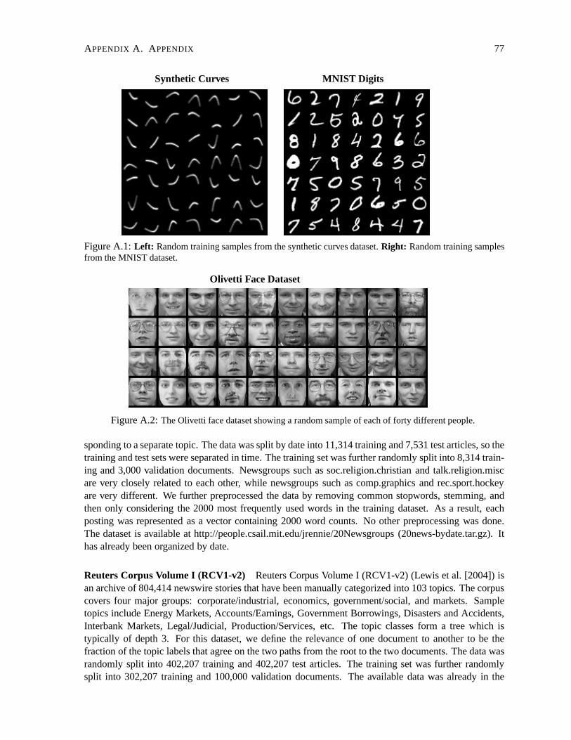
APPENDIX A. A PPENDIX 77
Synthetic Curves MNIST Digits
Figure A.1:Left: Random training samples from the synthetic curves dataset.Right: Random training samplesfrom the MNIST dataset.
Olivetti Face Dataset
Figure A.2:The Olivetti face dataset showing a random sample of each of forty different people.
sponding to a separate topic. The data was split by date into 11,314 training and 7,531 test articles, so thetraining and test sets were separated in time. The training set was further randomly split into 8,314 train-ing and 3,000 validation documents. Newsgroups such as soc.religion.christian and talk.religion.miscare very closely related to each other, while newsgroups such as comp.graphics and rec.sport.hockeyare very different. We further preprocessed the data by removing common stopwords, stemming, andthen only considering the 2000 most frequently used words inthe training dataset. As a result, eachposting was represented as a vector containing 2000 word counts. No other preprocessing was done.The dataset is available at http://people.csail.mit.edu/jrennie/20Newsgroups (20news-bydate.tar.gz). Ithas already been organized by date.
Reuters Corpus Volume I (RCV1-v2) Reuters Corpus Volume I (RCV1-v2) (Lewis et al. [2004]) isan archive of 804,414 newswire stories that have been manually categorized into 103 topics. The corpuscovers four major groups: corporate/industrial, economics, government/social, and markets. Sampletopics include Energy Markets, Accounts/Earnings, Government Borrowings, Disasters and Accidents,Interbank Markets, Legal/Judicial, Production/Services, etc. The topic classes form a tree which istypically of depth 3. For this dataset, we define the relevance of one document to another to be thefraction of the topic labels that agree on the two paths from the root to the two documents. The data wasrandomly split into 402,207 training and 402,207 test articles. The training set was further randomlysplit into 302,207 training and 100,000 validation documents. The available data was already in the
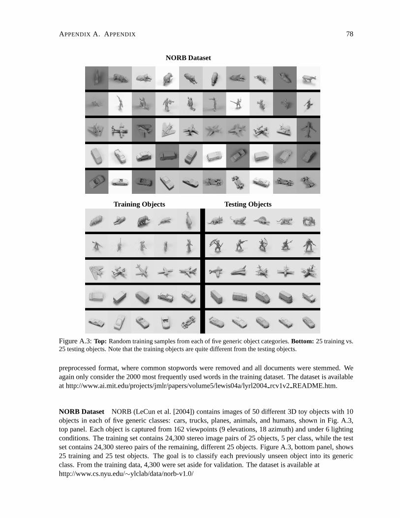
APPENDIX A. A PPENDIX 78
NORB Dataset
Training Objects Testing Objects
Figure A.3:Top: Random training samples from each of five generic object categories.Bottom: 25 training vs.25 testing objects. Note that the training objects are quitedifferent from the testing objects.
preprocessed format, where common stopwords were removed and all documents were stemmed. Weagain only consider the 2000 most frequently used words in the training dataset. The dataset is availableat http://www.ai.mit.edu/projects/jmlr/papers/volume5/lewis04a/lyrl2004rcv1v2 README.htm.
NORB Dataset NORB (LeCun et al. [2004]) contains images of 50 different 3Dtoy objects with 10objects in each of five generic classes: cars, trucks, planes, animals, and humans, shown in Fig. A.3,top panel. Each object is captured from 162 viewpoints (9 elevations, 18 azimuth) and under 6 lightingconditions. The training set contains 24,300 stereo image pairs of 25 objects, 5 per class, while the testset contains 24,300 stereo pairs of the remaining, different 25 objects. Figure A.3, bottom panel, shows25 training and 25 test objects. The goal is to classify each previously unseen object into its genericclass. From the training data, 4,300 were set aside for validation. The dataset is available athttp://www.cs.nyu.edu/∼ylclab/data/norb-v1.0/
APPENDIX A. A PPENDIX 79
A.2 Details of Training
Details of the pretraining: To speed up the pretraining of each RBM, we subdivided all datasetsinto mini-batches, each containing 100 data vectors and updated the weights after each mini-batch. Fordatasets that are not divisible by the size of a minibatch, the remaining data vectors were included inthe last minibatch. For all datasets, each hidden layer was pretrained for 50 passes (epochs) throughthe entire training set. The weights were updated using a learning rate of 0.1, momentum of 0.9, and aweight decay of0.0002×weight×learning rate. The weights were initialized with small random valuessampled from a zero-mean normal distribution with standarddeviation 0.01. When modeling real-valued Gaussian visible units, e.g. in the case of modeling Olivetti face patches, pretraining the firstlayer of features typically requires a much smaller learning rate to avoid oscillations. The learning ratewas set to 0.001 and pretraining proceeded for 200 epochs.
During the pretraining stage, the visible units of standardbinary RBM had real-valued activities,which were in the range[0, 1]. When training higher-level RBM’s, the visible units were set to theactivationprobabilitiesof the hidden units in the lower-level RBM, but the hidden units of every RBMhad stochastic binary values.
Details of the fine-tuning: For the fine-tuning, we used the method of conjugate gradients on largerminibatches containing 1000 data vectors. We used Carl Rasmussen’s “minimize” code, available athttp://www.kyb.tuebingen.mpg.de/bs/people/carl/code/minimize. Three line searches were performedfor each mini-batch in each epoch. To determine an adequate number of epochs and to check foroverfitting, we fine-tuned each model on a fraction of the training data and tested its performance on theremaining validation set. We then repeated the fine-tuning on the entire training set.
For many of the experiments presented in this thesis, we tried various values of the learning rate,momentum, and weight-decay parameters and we also tried training the RBM’s for more epochs. Wedid not observe any significant differences in the final results after the fine-tuning. This suggests thatthe precise weights found by the greedy pretraining do not matter as long as it finds a good region fromwhich to start the fine-tuning.
A.3 Details of Matlab code
Deep Autoencoders.The Matlab code for pretraining a stack of RBM’s using Contrastive Divergence(CD1) and fine-tuning deep autoencoders is available athttp://www.cs.toronto.edu/∼rsalakhu/software/.
Estimating Partition Functions of RBM’s. The Matlab code for estimating partition functions of RBM’susing Annealed Importance Sampling is available athttp://www.cs.toronto.edu/∼rsalakhu/software/.
Pretraining and Learning Deep Boltzmann Machines.The Matlab code includes: pretraining a mod-ified stack of RBM’s, the new learning algorithm that combines mean-field inference along withstochastic approximation algorithm, and discriminative fine-tuning of Deep Boltzmann Machines.The code is available at: http://www.cs.toronto.edu/∼rsalakhu/software/.


![A arXiv:1509.00519v4 [cs.LG] 7 Nov 2016 · Under review as a conference paper at ICLR 2016 IMPORTANCE WEIGHTED AUTOENCODERS Yuri Burda, Roger Grosse & Ruslan Salakhutdinov Department](https://static.fdocuments.net/doc/165x107/5ac335807f8b9a57528bd73e/a-arxiv150900519v4-cslg-7-nov-2016-review-as-a-conference-paper-at-iclr-2016.jpg)