by David D. Apsley, B. A. A Thesis submitted to The University of

Numerical Modelling of Neutral and Stably Stratified Flow and Dispersion In Complex Terrain

by

David D. Apsley, B. A.

A Thesis submitted to

The University of Surrey

for the degree of

Doctor of Philosophy

in the Faculty of Engineering

Department of Mechanical Engineering

University of Surrey

July 1995

Abstract

A three-dimensional finite-volume computer code (SWIFT) has been developed to predict

atmospheric boundary-layer flow and dispersion over complex terrain. Using a surface-

following, non-orthogonal coordinate transformation, with staggered velocity storage, the

primitive-variable conservation equations for mass, momentum and scalar transport are solved

iteratively by means of a pressure-correction algorithm. Means of accelerating the solution

of the pressure equation are examined.

The minimum level of turbulence closure appropriate to separated flows is two-equation

modelling. Variants of the k-E model to accommodate mean-streamline curvature and

streamwise pressure gradients have been coded and demonstrated to provide improved

performance in separated-flow calculations. It is shown how these models may be extended

naturally to three dimensions. A "limited-length-scale" k-c model is developed for atmospheric

boundary-layer applications. The model successfully reproduces the Leipzig wind-speed

profile and data from stable boundary-layer measurements at Cardington.

SWIFT has been appraised with respect to two experimental data sets for flow and diffusion

in complex terrain: the two-dimensional, neutrally stable, "RUSHIL" wind-tunnel study and

the Cinder Cone Butte field dispersion experiment. The former illustrates the capacity of

modified two-equation turbulence models to predict separation from curved bodies. The latter

demonstrates the utility of the length-scale-limiting technique and the ability to predict the

important features of strongly stratified shear flows around three-dimensional hills. Both

exercises show, however, that, whilst mean flow and vertical diffusion can be predicted, the

handling of lateral dispersion with an isotropic eddy diffusivity is generally unsatisfactory.

Various time-dependent features - including intermittent separation and wind direction

changes amplified by topographic blocking in strongly stratified flow - generate mean

concentration distributions significantly different from those which might be anticipated from

the time-averaged mean flow.

i

Declaration

No portion of the work referred to in this Thesis has been submitted in support of an

application for another degree or qualification of this or any other university or other institute

of learning.

11

Acknowledgements

I am grateful to all the people who enabled me to undertake and complete this research.

Foremost among these are my colleagues at the University of Surrey who provided a good

working environment and a very happy place to study. Particular tribute is paid to my

supervisor, Professor Ian Castro, for setting up the research project, guiding me throughout

and reading innumerable drafts of this Thesis.

A number of institutions contributed data for the numerical comparisons. Dr. W. H. Snyder

and Dr. R. S. Thompson at the US Environmental Protection Agency's Fluid Modelling

Facilities supplied the Milestone Reports of the Cinder Cone Butte dispersion study and the

Laboratory Report for the RUSHIL experiment. Analysed data from the latter experiment was

provided by Dr. F. Tampieri at FISBAT in Bologna. Thanks must also go to the UK

Meteorological Office and, in particular, to Dr. S. H. Derbyshire, for boundary-layer profiles

from the Cardington site and some useful discussions on stable boundary-layer modelling.

Financial support was provided by a research studentship from the Natural Environment

Research Council.

Finally, eternal thanks are due to my wife Judith for her constant love and support, and to my

baby daughter Miriam who arrived in the later stages of writing and prompted me to hurry

up and finish!

111

Nomenclature

a =7 77/k -2/38 anisotropy parameter

AP+d, aP+d (unnormalised and normalised) matrix coefficients in transport equations

Aa control-volume face area in curvilinear space

BP, bP (unnormalised and normalised) explicit source term in transport equations

C mean concentration

c =o)/k; along-wind phase velocity

cP specific heat capacity

cg =Vkw ; group velocity

cp phase velocity

CI,, CEIICE21GOCYCIße

constants in k-c turbulence model

D computational domain height

D$ , dý, (°`' (unnormalised and normalised) pressure coefficients in momentum equations

D[] integral divergence operator

D/Dt material derivative following the mean flow

f =2S2sinX; Coriolis parameter

F rate of production of turbulent kinetic energy by body forces

F, f integral flux and flux density vectors

F; ý rate of production of Reynolds stress by body forces

Fr Froude number

fµ, fl, f2 damping functions in low-Reynolds-number k-c model

G rate of production of turbulent kinetic energy by buoyancy forces

g gravitational acceleration

gi, natural and dual curvilinear basis vectors

g, metric tensor

Ga integrated mass flux through a control-volume face

H hill height

h

Hý

boundary-layer height

dividing-streamline height

inversion height

iv

hs source height

J Jacobian of transformation

k turbulent kinetic energy

k, l, m -or (k) wavenumber components

KM, KH eddy diffusivities for momentum and heat

L horizontal length scale

Q inner-layer depth of Jackson-Hunt theory

im mixing length

/c; dissipation length '

m(II

Cn In

maximum mixing length

Monin-Obukhov length

normal distance to wall

IV depth of viscous sublayer +« 1fl ý

l, t near-wall normalised length scales

N buoyancy frequency

n normal coordinate

P mean pressure

P

Pr

or

production of turbulent kinetic energy by mean shear

pressure perturbation in linearised flow models

molecular Prandtl number

PE production term in dissipation equation

Q source strength

QH heat flux

R ideal gas constant

r relaxation parameter

r position vector

Rc radius of curvature

Re =UL/v; Reynolds number

Rf (flux) Richardson number

Ri (gradient) Richardson number

Ro =U/fL; Rossby number

V

R1

S

s

S«', s(o)

Sll

SP

T

t U, V, W or (U)

tt, v, w or (u)

LlI , vI , bL'I or (ui')

U{ VR

U`, Ui

uo

UT or ý[*

Vý

W

Wg

x, 1", -- or (x, )

ýr

zs

ZO

a

PIP, F F. AM

OS

dý , 0ýý, ý.:.

=k2/ve; turbulent Reynolds number

=p 5ýý, ý; mean-strain invariant

streamline coordinate

(integrated and specific) source terms

mean rate-of-strain tensor

implicit source term in transport equations

temperature

time

Cartesian mean-velocity components

Cartesian mean-velocity perturbations in linearised flow models

turbulent velocity fluctuations

geostrophic velocity

contravariant and covariant velocity components

turbulent velocity scale

friction velocity

volume in curvilinear space

=U+iV; complex velocity

=U, +iVx; complex geostrophic velocity

Cartesian coordinates

plume height

surface height

roughness length

coefficient of expansion

constants in surface-layer similarity profiles; both =5;

general diffusivity

Christoffel symbol

mass of control volume

relative speed-up factor

grid spacing

vi

b =z-z-; streamline displacement

or

shift operator

8ý ) pressure-correction coefficient

F_ turbulent kinetic energy dissipation rate

O mean value of scalar (here, potential temperature)

O perturbation value of scalar

K von Karman's constant (=0.4)

KC curvature

Kg diffusivity

A,. 10 local Monin-Obukhov length

v (kinematic) molecular viscosity

vt eddy viscosity

4, rj, ý or (, ) curvilinear coordinates II =P+G: total production term in turbulent kinetic energy equation

p density

6 turbulent Prandtl number

6le 9ßv 9ßlti"

6I 6

2

TE

0

x 'I' sý

or

topographic shape factor

rms velocity fluctuations

plume crosswind spread parameters in lateral and vertical directions

shear stress

Reynolds stress

=k/e; eddy turnover timescale

general transported scalar

or

constant in algebraic stress model

pressure-strain correlation

=CUH2/Q; normalised concentration

stream function

angular velocity

(0 angular frequency

vii

W

Subscripts

=VAÜ; mean vorticity

a approach flow

f face value

p particular node

p+d node in direction d from p

00 upstream at infinity

viii

Contents

Abstract ....................................................... I

Declaration ..................................................... ii

Acknowledgements ............................................... iii

Nomenclature ................................................... iv

CHAPTER 1.

Introduction .................................................. 1-1

CHAPTER 2.

Literature Review and Background Theory ............................. 2-1

2.1 Experimental Measurements of Flow and Dispersion in Complex Terrain 2-1

2.1.1 Field Studies .................................... 2-2

2.1.2 Laboratory Simulation ............................. 2-5

2.2 Theoretical Models ...................................... 2-8

2.2.1 Linear Theory ...................................

2-8

2.2.2 Finite-Amplitude Models ...........................

2- 22

2.2.3 Low-Froude-Number Flows .........................

2- 27

2.2.4 Turbulent Flow Over Low Hills ...................... 2- 31

2.2.5 Dispersion Modelling in Complex Terrain ...............

2- 35

2.3 Numerical Modelling ....................................

2-40

CHAPTER 3.

The SWIFT Code ..............................................

3-1

3.1 Governing Equations ....................................

3-1

3.1.1 Mean Flow .....................................

3-1

3.1.2 Turbulence Models ...............................

3-4

ix

3.1.3 Non-Dimensionalisation ............................ 3-6

3.2 Numerical Methods ..................................... 3-8

3.2.1 Working Variables and Form of Equations ............... 3-8

3.2.2 Control-Volume Geometry .......................... 3-8

3.2.3 Transport Equations in Curvilinear Coordinate Systems ......

3 -9 3.2.4 Discretisation of the Scalar Transport Equation ............

3- 15

3.2.5 The Pressure Equation ............................. 3- 23

3.2.6 Advection Schemes ...............................

3- 25

3.2.7 Solution of Matrix Equations ........................

3- 30

3.2.8 Handling of Equation Coupling .......................

3- 33

3.2.9 Topographic Coordinate Transformation in SWIFT ......... 3- 37

3.2.10 Bluff-Body Blockages in SWIFT .....................

3- 38

3.2.11 Boundary Conditions ............................. 3- 39

3.2.12 Imbedded Analytical Domain Method For Isolated Releases .. 3- 40

CHAPTER 4.

Turbulence Modelling ........................................... 4- 1

4.1 A Hierarchy of Turbulence Models ..........................

4- 1

4.1.1 Second-Order Closure .............................

4-2

4.1.2 Algebraic Stress Models ............................ 4- 6

4.1.3 Eddy-Viscosity Models ............................

4-9

4.2 Modifications to the Standard k-c Model ......................

4- 12

4.2.1 Low-Reynolds-Number k-c Models .................... 4- 12

4.2.2 Non-Linear k-c Models ............................

4- 15

4.2.3 Streamline Curvature Modification ....................

4- 18

4.2.4 Preferential Response of Dissipation to Normal Strains ...... 4- 22

4.3 Near-Wall Modelling By Wall Functions ...................... 4- 24

CHAPTER 5.

Atmospheric Boundary-Layer Modelling ...............................

5-1

5.1 Atmospheric Boundary-Layer Equations .......................

5-2

5.1.1 Mean-Velocity Equations ...........................

5-2

X

5.1.2 Mean Temperature Profile and the Effect of Buoyancy Forces .5-5

5.2 Surface-Layer Similarity Theory ............................ 5-8

5.3 Local Scaling: Nieuwstadt's Model .......................... 5- 11

5.4 Other Atmospheric Boundary-Layer Closure Models .............. 5- 15

5.5 A Limited-Length-Scale k-E Model .......................... 5- 18

5.5.1 Neutral Atmospheric Boundary-Layer Simulation .......... 5- 23

5.5.2 Stable Atmospheric Boundary-Layer Simulation ........... 5-25

5.5.3 Comparison With Cardington Data ....................

5- 30

CHAPTER 6.

Comparison With Experiment ...................................... 6- 1

6.1 The Russian Hill (RUSHIL) Wind-Tunnel Study ................. 6-2

6.1.1 Summary of the Wind-Tunnel Study ...................

6-2

6.1.2 Summary of the Flow Calculation .....................

6-3

6.1.3 Flow Comparison ................................

6-5

6.1.4 Concentration Comparison .......................... 6- 10

6.2 The Cinder Cone Butte Field Dispersion Experiment .............. 6- 14

6.2.1 Setting Up the Simulation .......................... 6- 17

6.2.2 Flow Features ................................... 6- 22

6.2.3 Concentration Calculations ..........................

6- 25

CHAPTER 7.

Conclusions and Further Research ...................................

7-1

Bibliography .................................................. B-I

Tables are imbedded in the text near the point of reference. Figures are to be found at the end

of each Chapter.

xi

To my parents,

whose love and industry in raising me knew no bounds.

CHAPTER 1.

Introduction

Topographic effects on air flow are important in many situations. Speed-up and enhanced fluctuations must be accounted for when assessing wind-energy resources and wind loading

on structures. The transport of airborne pollutants is affected by changes to both mean wind

and turbulence, as is the movement of dust and sand. In forestry and agriculture, concern

about crop damage and fire propagation create a need for wind-field modelling. The forced

vertical displacement of saturated air gives rise to orographic rainfall. At larger scales,

topographic drag forms a substantial part of the momentum budget of the atmosphere and is

a major input to weather forecasting and climate models.

Atmospheric flows are complicated by buoyancy and Coriolis forces. A strong coupling may

exist between these body forces and the flow perturbations due to topography. Stable or

unstable stratification often occurs as a result of differences in temperature between the

surface (heated or cooled by radiation) and the air aloft. Vertical motions are enhanced by

unstable stratification and diminished by stable stratification. In complex terrain stable

stratification results in internal gravity waves and katabatic (downslope) winds. Numerically,

stably stratified flows are harder to handle than neutral flows, since turbulent transport is

smaller (and, in practice, often intermittent), resulting in steeper flow gradients.

Heavy industry is often situated in complex terrain for good socio-economic reasons: an

abundant supply of water, the availability of land unsuitable for agriculture and the need to

minimise the visual impact or environmentally detrimental emissions of the plant. Some

important utilities may be located in mountainous areas for strategic reasons. However,

industry cannot always be remote from the population that it serves and there is an urgent

need for means of assessing the local impact of routine or accidental emissions of airborne

pollution.

The prediction of air flow and/or diffusion in complex terrain may be based on experimental

or theoretical techniques. Experimental measurements can be made at full scale or in the

1-1

laboratory, whilst theoretical modelling ranges from empirical formulae to analytical methods

to full numerical solution. Table 1.1 identifies some of the advantages and disadvantages of

each method. A more satisfactory assessment is obtained from a combination of approaches,

rather than a single means in isolation, since each makes some modelling assumption. (In the

case of full-scale experiments this is that a limited number of site-specific measurements can

supply an adequate statistical database on which to build an environmental assessment. ) It has

become increasingly common to find one approach being used to validate another.

Advantages Disadvantages

Experiment Full-scale "Real" flow and geometry. Expensive. Public acceptance of results. Limited resolution.

No control over cases covered. Site-specific.

Laboratory Complex site investigations Truncated domain. before construction. All scale-similarity Control of flow parameters. requirements cannot be met Good resolution. simultaneously.

Theory Empirical Cheap and quick. Little or no physics. User-friendly. Requires extrapolation from Rapid response in data by which it is calibrated. emergency. Probabilistic risk assessment with large matrix of cases.

Analytical Fairly quick and Approximation and modelling inexpensive. assumptions necessary. Some physics involved. Idealised input conditions. Realistic topography.

Numerical Flexible geometry. Discrete, truncated domain. Fully non-linear. Modelling assumptions Control of inflow conditions necessary. and output type/location. Requires large computers for Can isolate different physical three-dimensional topography. effects.

Table 1.1: Advantages and disadvantages of different approaches to the prediction of atmospheric boundary-layer flow and diffusion.

In Great Britain and the United States the power-generation utilities have been at the forefront

of experimental investigation into the near-field dispersion of pollution, particularly with

regard to effects arising from the proximity of large buildings or complex terrain. Research

has been conducted to assess the extent to which wind-tunnel and theoretical modelling can

reproduce the ground-level concentrations arising from tracer-release experiments conducted

at power-station sites. The further development and application of remote-sensing techniques,

such as SODAR and LIDAR, will, undoubtably, increase our knowledge of atmospheric

boundary-layer structure and its effect on diffusing clouds.

Laboratory simulations of atmospheric flow and diffusion have been conducted in wind

tunnels and in water flumes or towing tanks. The increasing importance of pollution-

dispersion assessment as opposed to wind-loading studies has prompted the development of

facilities for simulating density stratification effects (Snyder, 1979,1990, Rau et al., 1991,

Castro and Robins, 1993). In the wind tunnel (as in the atmosphere) this is achieved by

differential heating (or cooling), whilst in water channels salt concentration can be used to

create density variations.

Empirical models of diffusion - the majority based on some form of gaussian-plume model - have long been the tools of the trade in environmental impact assessment. They are

invariably used where large numbers of cases have to be considered - for example, in

probabilistic risk assessment. The basic parameters consist of a plume trajectory - typically

a straight line, although, in some cases, modified to account for topographic undulations or

buoyant plume rise - and horizontal and vertical crosswind plume spreads 6, and 6,, specified

as functions of downwind distance. The rate of plume spread in the horizontal and vertical

depends primarily on atmospheric stability. New models (eg, Hunt et al., 1990), based on a

better understanding of boundary-layer structure and using linearised flow models to compute

trajectories in complex terrain, are beginning to supplant earlier schemes based only on

surface-layer meteorology and empirical adjustments to plume height. However, these are still

fundamentally unsound in highly non-linear regions of the flow - for example, within

separated recirculation zones - and in circumstances where the narrow-plume assumption is

untenable.

Theoretical modelling of flow over topography has proceeded along a number of fronts.

Linearised theory has been applied to boundary-layer flow over low hills (Jackson and Hunt,

1975; Taylor et al., 1983; Beljaars et al., 1987) and to the generation of internal gravity waves (Smith, 1980; Hunt et al., 1988). Two-dimensional finite-amplitude stratified flows can be

treated by Long's model (Long, 1952; Yih, 1965), whilst Drazin's asymptotic theory (Drazin,

1961; Brighton, 1978) provides for horizontal potential flow around three-dimensional hills

in the strongly stratified limit. At intermediate Froude numbers, however, there are substantial

gaps which no analytical theory has managed to fill.

Recent increases in computer power mean that numerical prediction of flow in complex

terrain is now viable: examples include finite-volume calculations for the Askervein hill

(Raithby et al., 1987) and Steptoe Butte (Dawson et al., 1991). A later Chapter of this Thesis

will describe the numerical prediction of stably stratified flow and dispersion around Cinder

Cone Butte, an isolated hill in Idaho. Computational fluid dynamics is being used extensively

to identify specific effects such as severe downslope wind storms and high-drag states,

associated with the breaking of topographically-forced non-linear gravity waves (Bacmeister

and Pierrehumbert, 1988), and conditions for upwind stagnation in highly stratified flows

around three-dimensional hills (Smolarkiewicz and Rotunno, 1990). The last has more than

a passing relevance to the dispersion of pollution because it represents a circumstance in

which a plume of material may impinge directly upon the surface.

Numerical modelling cannot be dissociated from underlying turbulence models, particularly

where it is required to compute pollutant dispersion as well as the mean flow field. Second-

order closure has been reviewed by Launder (1989) and Hanjalic (1994). However, the

resources required to undertake fully three-dimensional computations for real terrain often

make it necessary to resort to lower-order closures, the commonest being eddy-viscosity

models. These must be "optimised" for each type of flow, but it is possible to modify them

to admit specific effects, such as streamline curvature, guided by a general picture of

turbulence structure over hills provided by experiment (Mickle et al., 1988) and higher-order

closure (Zeman and Jensen, 1987).

Having indicated situations where topographic effects are important, summarised the practical

means of modelling them and identified areas where numerical modelling would be beneficial,

the structure of this Thesis may now be outlined.

The primary aims and objectives of this research are:

" to evaluate and/or develop turbulence models for the prediction of neutral and stably

stratified atmospheric boundary-layer flow and dispersion over complex terrain;

" to develop a computer code for the prediction of the same around arbitrar}

topography;

" to evaluate the performance of this numerical tool in relation to existing experimental

databases.

It is in the very nature of research that the original aims and objectives invariably change -

at least in emphasis - throughout the duration of a project. That the key objectives above have

been met will, nonetheless, be apparent in the work that follows.

Chapter 2 provides an extensive review of published literature and background theory with

regard to the measurement and modelling of flow and dispersion around topography.

Additional material more directly related to turbulence modelling practice and, in particular,

its application to the atmospheric boundary layer, is reserved to the appropriate later Chapters

(4 and 5).

The major product of this research is the computer code SWIFT -a rather contrived acronym

for Stratified WInd Flow over Topography. The work involved extending an original two-

dimensional, laminar, cartesian-geometry code to one capable of computing three-dimensional

flows, with various turbulence models and a terrain-fitting curvilinear coordinate system for

the incorporation of arbitrary (smooth) topography. The numerical methods embodied in

SWIFT are described in Chapter 3.

Turbulence modelling is reviewed in Chapter 4 and the extent to which second- and lower-

order closures can model the anisotropic forcing present in atmospheric flows is examined.

Modifications to eddy-viscosity models to account for mean-streamline curvature and

streamwise pressure gradients in two-dimensional flows are extended naturally to three

dimensions. Both features are invariably met in flow over obstacles.

Chapter 5 deals specifically with turbulence modelling in the atmospheric boundary layer.

After a review of similarity approaches for the surface layer and stable boundary layers a new

variant of the k-E turbulence model is presented, for circumstances where the mixing length

is limited by some non-local constraint - for example, the boundary-layer depth or a stability

length scale.

In Chapter 6 the SWIFT code is appraised with respect to two experimental databases for

flow and dispersion over hills. The first - the "Russian Hill" study of Khurshudyan et al.

(1981) - is a wind-tunnel study of neutrally stratified flow and diffusion over a series of two-

dimensional hills with different slopes. The second test case is the field study of the United

States Environmental Protection Agency at Cinder Cone Butte in Idaho (Lavery et al., 1982).

where tracer experiments were conducted with upwind sources in highly stable flow.

Chapter 7 summarises the findings of the research and the performance of the theoretical

models and computational tools. It also makes recommendations of areas for future study.

CHAPTER 2.

Literature Review and Background Theory

The purpose of this Chapter is to summarise previous work on flow and dispersion in

complex terrain and, where appropriate, to develop some of the theory. A brief introduction

is necessary to permit the reader to navigate the various strands.

This review is subdivided into three main topics: experimental measurements, analytical

theory and numerical computation. The equally important subjects of turbulence modelling

and the structure and simulation of the atmospheric boundary layer are treated in Chapters 4

and 5 respectively, where further literature related to these will be reviewed.

In Section 2.1 the selection of experimental measurements is divided into field and laboratory

studies. In Section 2.2 we review various analytical models for neutral and stably stratified

flow and dispersion over surface topography. The first three are essentially inviscid: linear,

finite-amplitude and low-Froude-number theories. The fourth considers turbulent shear flow

over low hills of the form typified by Jackson-Hunt theory. The last subsection summarises

existing dispersion models for routine and regulatory use. Finally, in Section 2.3 we consider

numerical modelling of flow and dispersion in complex terrain.

2.1 Experimental Measurements of Flow and Dispersion in Complex Terrain

Although a qualitative description of airflow in complex terrain had been extant for some

time, Jackson and Hunt (1975) provided the first satisfactory theory matching the outer-layer

disturbance caused by streamline displacement over undulating terrain with the turbulent shear

layer near the ground. Although the model has since been refined and extended, the central

premise still stands -a division of the flow into an outer layer, where the flow perturbation

is essentially inviscid (driven by pressure fields generated by streamline displacement). and

an inner layer, where the turbulent shear stress is important and is described by a mixing-

length model. We shall examine this theory in greater detail later.

In their challenging 1975 paper, Jackson and Hunt not only established a firm foundation for

future theoretical development, but emphasised the need for experimentalists to provide them

with data with which to validate their model. Since then, a large number of experimental

studies - both in the field and in the laboratory - have been instigated. An excellent review

of the full-scale measurements has been given by Taylor et al. (1987).

2.1.1 Field Studies

Perhaps the first full-scale experimental study specifically designed to test the predictions of

Jackson-Hunt theory was that of Mason and Sykes (1979a) at Brent Knoll in Somerset. In the

same paper the authors presented the natural extension of the original two-dimensional theory

to three dimensions, so opening up the practical application of the model to real terrain.

Measurement detail was comparatively limited, being restricted to mean wind speed

measurements at 2m above the surface. Nevertheless, it did allow an assessment of the global

predictions of the model - such as the maximum speed-up at the summit - to be made. The

British Meteorological Office followed this up with more detailed measurement programmes

at other isolated hills: the island of Ailsa Craig (Jenkins et al., 1981), Blashaval (Mason and

King, 1985) and Nyland Hill (Mason, 1986).

Meanwhile, on the other side of the world, CSIRO were making use of a redundant television

mast to make measurements of mean and turbulent wind profiles over the summit of Black

Mountain, near Canberra (Bradley, 1980). A local velocity maximum or "jet" was observed

at a height and of a magnitude consistent with Jackson-Hunt theory, despite the manifest

violation of the low-slope, two-dimensional assumptions of that model. The influence of

(weak) thermal stability and non-normal wind incidence angles were investigated in a follow-

up study at Bungendore Ridge (Bradley, 1983). Observations showed that the maximum

speed-up factor, AS=(U(z)-U�(z))IU�(z), varied in a manner consistent with changes to the

approach-flow mean wind speed profile occasioned by stability. According to Jackson-Hunt

theory,

A Smax D U(Q) QH

U(L) U(Q) L( U(Q)

(2.1)

where H is the height of the hill, L the half-length (average radius from the summit of the "2H

contour), Q is the inner-layer height (see later) and 6 is a shape factor of order unity. The

approach-flow mean wind speed may (at least in the surface layer) be described by Monin-

Obukhov similarity theory (Chapter 5):

u U(z) [ln(z/zo) +5z/LMO] (2.2)

giving a characteristic variation in the maximum speed-up as the Monin-Obukhov length

varies. The study also flagged the importance of a roughness transition over the hill, a feature

to which we will return later. More recently, the same organisation has made a more detailed

series of measurements examining the effects of thermal stability at Coopers Ridge (Coppin

et al., 1994).

Probably the most detailed of all wind-field measurement programs was undertaken at

Askervein, a 116m-high hill on South Uist in the Outer Hebrides, as part of an International

Energy Agency program on research and development into wind energy. Spatial resolution

was obtained from several linear arrays of anemometers at 10m from the ground,

supplemented by profile data from fixed masts up to 50m in height at key locations, including

the summit and a reference site upwind. Further TALA kite and airsonde releases provided

some wind measurements at greater heights. An overview of the experiment can be found in

Taylor and Teunissen (1987), analysis of the spatial variation of wind speed in Salmon et al.

(1988) and profile data in Mickle et al. (1988). This was a remarkable project because the

program also included wind-tunnel simulations at three scales (Teunissen et al., 1987) and a

finite-volume calculation (Raithby et al., 1987).

A number of full-scale measurements of atmospheric dispersion have also been carried out

in regions of complex terrain. These include both monitoring studies for existing industrial

pollution sources - such as power stations and incinerators - and deliberate releases near

isolated terrain features to study generic effects. Even in the former case it is common to

inject and track an artificial tracer, since this eliminates errors due to natural background and

uncertainty in the source strength. The tracers used must be stable, non-toxic and detectable

at low concentrations. Sulphur hexafluoride (SF6) and the halocarbons CZCI4 and CH, Br have

been widely used. Most quantitative studies have focused on ground-level concentrations,

although advances in remote sensing technology - in particular, the development of LIDAR

(Laser Interferometry Detection And Ranging) - now permit the resolution of vertical plume

structure. The mobility of vehicle-mounted instrumentation also has benefits over fixed

sampling arrays when the ambient wind direction is unreliable.

Maryon et al. (1986) followed up the earlier flow measurements by Mason and King (1985)

at Blashaval with a point-source diffusion study in neutral conditions. A limited sampling

array on the upwind slope was able to measure crosswind spread and vertical plume profiles

up to 15m (for a source height of 8m). Concentration measurements were consistent with flow

divergence in the horizontal and convergence in the vertical, bringing the plume closer to the

ground. Building on experience gained from this study, the UK Meteorological Office carried

out a second dispersion study in neutrally stable conditions at Nyland Hill (Mylne and

Callander, 1989). In this experiment dual tracers were emitted simultaneously from two

heights. Plume crosswind spread confirmed the effects of flow divergence and was greater for

the lower source.

The effect of horizontal divergence is greater in stably stratified flows, where vertical

deflection of streamlines is suppressed by buoyancy forces. A number of well-documented

studies have been carried out in the United States to characterise dispersion from upwind

sources in strongly stable flow. These include the EPA Complex Terrain Model Development

Program experiments at Cinder Cone Butte and Hogback Ridge (Strimaitis et al., 1983). The

first of these will be discussed in more detail in Chapter 6, where the results of a numerical

comparison are presented. Dispersion studies were also conducted by Ryan et al. (1984) at

the much higher Steptoe Butte (340m). In this experiment tracer gases were released (from

a tethered balloon support) at heights up to 190m. These measurements demonstrated

considerable sensitivity to wind direction in flows for which Fr<1 (where Fr-U/NH is the

Froude number based on hill height), with strong lateral divergence and, in many cases, plume

impaction on the surface. They also confirmed the usefulness of the "dividing-streamline

2-4

height", a representative height determined from the approach-flow velocity and density

profiles which, on energy grounds, distinguishes fluid with sufficient kinetic energy to

surmount the hill from that which must pass around the sides. We shall consider this concept in more detail below.

2.1.2 Laboratory Simulation

Laboratory simulation of environmental flow and dispersion is seen as an attractive alternative

to full-scale field experiments, particularly where a large matrix of inflow conditions and/or

source configurations are to be investigated. The commonest types of facility are wind tunnels

and water channels/towing tanks, with rotating tanks to investigate larger scale phenomena

where the effect of the earth's rotation becomes important. For atmospheric flows, recognition

of the importance of buoyancy forces has led to the development of facilities for simulating

density changes in the flow - thermally stratified wind tunnels and salinity-stratified towing

tanks. The similarity criteria which must be met in such scale simulations have been reviewed

by Snyder (1972) and Baines and Manins (1989).

The development of a quasi-equilibrium, deep turbulent boundary layer within a short fetch

is something of an art in itself. A common configuration uses a combination of low-level trip

and upright tapered elements at inflow, together with an artificially roughened floor (Robins,

1977). The wind-tunnel roof imposes a blockage effect which is not to be found in the

unbounded atmosphere. There is an outstanding controversy as to whether a zero-pressure-

gradient condition (obtained by locally raising or lowering the wind-tunnel roof) is the

appropriate means of eliminating this effect over two-dimensional topography.

Two effects complicating interpretation of results and the maintenance of steady conditions

in a towing tank which are not present in the real atmosphere are described by Snyder et al.

(1985). The first is the "squashing" or "blocking" phenomenon, whereby incompressible fluid

is obliged to pile up ahead of an obstacle by the finite length of the tank, returning over the

top to alter permanently the upstream density profile. The second results from the finite depth

of the tank supporting upstream-propagating columnar modes, which may, in their turn, reflect

from the upstream boundary. In the atmosphere, upward-propagating gravity waves radiate

to infinity, whereas, in a towing tank, they are reflected from floor or free surface. Baines and Hoinka (1985) describe a novel means of overcoming this in the laboratory by partitioning

their towing tank lengthways and deflecting outgoing waves out of the working side by means

of an angled plate.

A number of investigations have been carried out specifically to correlate the results of

laboratory and full-scale experiments. These include detailed comparisons for Gebbies Pass

(Neal, 1983) and the Askervein project (Teunissen et al., 1987). In the latter case, wind-tunnel

experiments were carried out at three scales. Snyder and Lawson (1981) describe towing-tank

simulations of the Cinder Cone Butte dispersion study. Wind-tunnel simulations of complex

terrain have been used extensively in planning studies for large industrial plant. To date, the

majority of wind-tunnel simulations of real terrain have been conducted in neutral stability.

A recent exception is the simulation of stably stratified flow around Mt Tsukuba in Japan

(Kitabayashi, 1991) using distorted vertical scaling.

Whilst detailed topographic models are undoubtably necessary for site-specific studies, they

are time-consuming and expensive to manufacture and do not readily lend themselves to a

fundamental understanding of the flow. For these reasons the majority of wind-tunnel

simulations have concentrated on simpler generic shapes. Bowen and Lindley (1977)

examined the speed-up over escarpments of various shapes, whilst Pearse et al. (1981) and

Arya and Shipman (1981) measured deep boundary-layer flow over two-dimensional ridges.

Arya et al. (1981) followed this up with measurements of diffusion from a point source in the

same flow. Castro and Snyder (1982) measured concentrations from sources downwind of

finite-length ridges and a cone. Their experiments were extended to non-normal wind

incidence by Castro et al. (1988). For dispersion around three-dimensional conical hills, Arya

and Gadiyaram (1986) and Snyder and Britter (1987) reported measurements of dispersion

from downwind and upwind sources respectively.

Among the general conclusions to be drawn from these studies about topography-affected

dispersion in neutral conditions are that, for upwind sources, the terrain amplification factor

(le, the relative increase in maximum ground-level concentration over the flat-terrain case)

is likely to be less for two-dimensional than three-dimensional topography. since. in the

former case, the streamlines pass further from the hill. For downwind sources, the reverse is

true, since two-dimensional flows exhibit stronger downwash - with or without flow

separation. The effect of this downwash - caused by a net downflow of fluid as the velocity

recovers in the wake - may lead to significant terrain amplification factors. Castro and Snyder

(1982) report values of 1.5 - 3.0 even for sources downwind of the separated-flow

reattachment point.

Of greater practical significance for real terrain are flow and dispersion measurements over

curved hills. (These represent a greater challenge in turbulence modelling and numerical

simulation since, unlike bluff body shapes, neither the onset nor the location of flow

separation is determinable from the geometry. ) Britter et al. (1981) studied slope and

roughness effects over two-dimensional bell-shaped hills, whilst Khurshudyan et al. (1981)

and Snyder et al. (1991) made detailed flow and dispersion measurements around isolated

two-dimensional hills ("RUSHIL" experiment) and the inverted valley configuration

("RUSVAL" experiment). Data from the RUSHIL experiment will be simulated using the

SWIFT code in Chapter 6. Gong and Ibbetson (1989) and Gong (1991) reported flow and

dispersion measurements over two- and three-dimensional hills of cosine-squared cross-

section.

Towing-tank experiments on stably stratified flow around axisymmetric hills were conducted

by Hunt and Snyder (1980). These investigated the range of application of Drazin's (1961)

low-Froude-number theory and how the lee-wave structure affected separation behind the hill.

In the latter aspect, they found that separation was boundary-layer controlled when the lee

wavelength 2itU/N was much longer than the length of the hill, but was totally suppressed

when the two were of the same order. As Froude numbers were reduced even further,

separation under a downstream rotor was provoked by the lee-wave field.

2.2 Theoretical Models

2.2.1 Linear Theory

Few would argue that the least tractable feature of the Navier-Stokes equations is their

inherent non-linearity. Since exact analytical solutions are seldom available, it is a common,

and not unreasonable, practice to see how far one can get by linearising the equations of

motion.

The small-perturbation analysis was developed for wave motions and the classical instability

problem by such "giants" of the last century as Stokes (1847), Lord Kelvin (W. Thompson)

(1879) and Lord Rayleigh (1880). At the turn of the century. Ekman (1904) was explaining

the increased drag on ships by means of internal gravity waves developed on the interface

between fresh and saline water in coastal regions. (A nice photograph of his laboratory

simulation can be found in Gill, 1982, p124. ) The analysis of discrete layers was extended

to the continuously stratified case by, amongst others, Lord Rayleigh (1883), although it was

papers by Brunt (1927) and his Norwegian counterpart Väisälä which brought to meteorology

what had already been well developed by the naval architects.

Important solutions for linear internal waves forced by topography in an unbounded

atmosphere were obtained by Lyra (1943) and Queney (1948), whilst Scorer (1949) extended

the uniform-velocity results to include the effects of upstream velocity shear. We shall

examine his equation in more detail below. One of the most important principles of linearised

theory is that of superposition, enabling the perturbation for arbitrarily shaped topography to

be generated from the integral sum of individual Fourier modes. Whilst straightforward to

derive analytically (Crapper, 1959), the general picture of disturbances arising from three-

dimensional topography is considerably more complex than its two-dimensional counterpart.

The lee-wave structure has been examined by Sawyer (1962). Smith (1980) presents an

excellent picture of the three-dimensional flow fields forced by topography and discusses the

effect of the hydrostatic assumption on near-surface and far-field perturbations to the flow.

The linear analysis is reworked in isosteric coordinates in Smith (1988). Although the

hydrostatic approximation is widely used as a simplifying assumption, its validity for typical

atmospheric profiles is often questionable (Keller, 1994).

Whilst many analytical results have been obtained for specific stability profiles (and the

uniform-velocity, constant-density-gradient situation is about the most commonly analysed and

least realistic of them), actual velocity and temperature profiles may exhibit considerable

variation. One of the most useful tools for analysing disturbances in non-uniform stratification

is ray-tracing (Lighthill, 1978).

Having given due credit to historical precedence we shall now examine mathematically some

of the results of linearised theory.

For small-amplitude disturbances to a Boussinesq, inviscid fluid with plane-parallel velocity

profile Ü(z)=(U(z), 0,0) and density profile pa(z), the continuity and momentum equations and

the incompressibility condition are, respectively,

V. u =0 (2.3)

Du- PO Dt

+ wd ZU-

-OP + Pg

Dp + wdpa

Dt dz 0

(2.4)

(2.5)

where d, p and p are the perturbation velocity, pressure and density fields and D=ö+ --

where Dt ät is the material derivative following the undisturbed flow.

Applying the operator VA(VA )=V(V' )-V2 to the momentum equation and taking the

resulting vertical component gives

D02w_d2Uaw Dt dz2 ax -gphP

Po (2.6)

which, on using the incompressibility equation to eliminate p, leads to an equation for the

vertical velocity component w:

2-9

D DV2w _d

2U aw + N2ýw =0 Dt Dt dz 2 ax

(2.7)

d 1/2

where N= -g po dz -

is the buoyancy or Brunt-Väisälä frequency. Since this equation is

homogene us and linear, with coefficients which are functions of Z only, it can be Fourier-

transformed in horizontal coordinates and time. Considering a single harmonic component

w(z; k, l, w)e`( +ay-"t), equation (2.7) is equivalent to the following equation in Fourier space:

a2w 1 d2U N2 y_v +

aZ2 U-CdZ2 (U-C)2

where c=w/k is the along-wind phase velocity.

k2 k2+12

w=0 k2

The primary applications of equations (2.7) or (2.8) are to

" hydrodynamic stability;

" internal waves forced by topography.

We shall examine each of these in turn.

(2.8)

Firstly, the hydrodynamic stability problem. For the harmonic component w(z)e i[k(x-ct)+ly] (with

the implicit dependence of w on wavenumber and frequency dropped for clarity), a growing

disturbance or instability is distinguished by c, -=Im(c)>O.

N is the frequency of small-amplitude oscillations of a particle displaced vertically in a

stratified fluid. The relative strength of buoyancy and shear may be expressed by the gradient

Richardson number Ri, the (squared) ratio of shear to buoyancy timescales:

N2 KI =

dÜ12 (2.9)

dz

According to a result conjectured by G. I. Taylor and first proved by Miles (1961), a necessary

condition for instability (a precursor to turbulence) for a plane-parallel shear flow is that Ri<'/4

somewhere in the flow. This paper in the Journal of Fluid Mechanics was followed by an

alternative proof by Howard (1961), which is so appealingly neat that it is worthwhile

2-10

repeating (in the current notation and extended to three dimensions) here. Making the

substitution H= -w in (2.8), one obtains

a( U_C)2naH aZ aZ

(U-C)n

+

{(U_C)2n-2[fl(fl

- 1) dU 2+N2 k2+12

J+(U_C)

2n- dz k2

=o

(n_1)d 2U

U-c)2n(k2+12) H dz 2

1 (2.10)

Multiplying by the complex conjugate 77 and integrating, this can be rearranged to give

f LzrU_Cl2n

Z1 J ax

az

2

+(k2+12) H a dz

Z +

f(u_c)2n-1(1 Z2_nld 2U

IH 2dZ

l Jdz

2

+ f(u_c)221n(1 Z_n)

_N2 k 22l2

1 dz k Hý2dz=0

(2.11)

(The first term has been integrated by parts, assuming w to vanish on z, and Z,, which may

be at ±-. )

Choosing n=1/2, and taking imaginary parts, we obtain

-ci f Z2

Z, ax coz

2+ (k2+12) IHI2 + N2 k2+12

_1 dU 2 IHI2 dz =0

(2.12) k2 4 dz U_c 2

z Hence, if Ri=

(dUN/dz)Z >41 everywhere then c; must be zero; ie, there is no instability. QED

As a side benefit, if we choose n=0 instead then we can derive another important result in

hydrodynamic stability. Imaginary parts give

fz2(d2U -2

k2+12 UC

ý2N dz zl dz2 k2 1 U-c IZ U-c 2

(2.13)

and hence a necessary condition for instability (non-zero c) is that

d2U - 2N2 k2+12 U-c

dz2 k2 JU-c r (2.14)

changes sign somewhere. This is a (rather unhelpful) extension to the stable case of Lord

Rayleigh's uniform-density result that a necessary condition for instability is that the mean-

velocity profile shall have an inflexion point: d2U/dz2=0.

The more important application for our present purposes is that of deriving the flow

perturbation forced by isolated topography. In this case the forcing is derived from the lower

boundary condition that the hill surface be a streamline: (Ü+u). V[z-Hf(x, y)] =0. On the

assumption that the hill height H is much less than a typical horizontal length scale, this

linearises to

w= UH! y

on z =0 ax

or, in Fourier space,

w(0) = ikUHf

(2.15)

(2.16)

Referring to equation (2.8), we see that, in two dimensions, an approach flow with mean- N2

velocity shear can be treated formally in the same way as unsheared flow, with N21d2U U-c

replaced by S2(z)= - U-c U-c dz 2. However, no such wavenumber-independent

simplification is possible in three dimensions, where (k2+1)/k2#1. To make the problem

tractable in three dimensions, then, we shall confine the analysis to the unsheared case,

U=constant.

To emphasise the wave nature of the solution, equation (2.8) can be written

_ +m2w=0 aZ 2

where

(2.17)

2- 12

m2 = -1

(k2+12)(k2+12+m2) ' (k2+12)(k2+12+m2) ' k2_12+m2

(ka+l2) ýý. 18)

For uniform N, equation (2.17) admits wavelike solutions w= {e "nZ, e if 1112 >0 and

exponential solutions w= {el in Lz, e - Im Iz } if m2<0. (In this context, {, } means "a linear

combination of". ) For the wavelike solutions one has a dispersion relation (inverting (2.18)):

w=k U-T N, I

with group velocity Cg = Ok (il

k2+12 k2+12+m2

(2.19)

"I nn\

Ü- U-c) k2m 2' klm 2' -km ý (k2+12)(k2+12+m2) (k2+l2)(k2+12+m2) k2--12+m2

Again, c=w/k is the along-wind phase velocity. The group-velocity vector cg determines the

rate and direction of wave-energy transport. (See Lighthill, 1978, for an excellent justification

of this interpretation. )

In a uniform, unbounded atmosphere a steady-state (c=0) solution of (2.17) satisfying the

lower boundary condition exists, with

w= woe'mz , wo=ikUHf (2.21)

where

m

I

i(k2+12)1iz

sgn(k) (k 2+

N >U

kI< N U

(2.22)

For large wavenumbers (short wavelengths) the solution is that which decays (exponentially)

with height. For small wavenumbers (long wavelengths) the wavelike solution is that for

N2 (kU-W)2

1- rk lz

1

Sgn(k)(ka+la)1iz N2 kU

2- 13

which the radiation condition (c,, _,

dw/dm>O) holds; ie, only outgoing wave energv ý permitted. From (2.20) this requirement amounts to mk>0, fixing the sign of in. The

wavelength 2iU/N which distinguishes the two cases is that of a fluid particle undertaking

oscillations of frequency N/2it whilst travelling at downwind speed U.

To consolidate we require expressions for the other flow variables. From the linearised

equations (2.3) - (2.5), assuming a stationary solution with spatial dependence e"`+' We have, from the horizontal momentum equation,

ü

V

P poU

lp (-).? 3)

k paU

which, combined with the continuity equation, give

w= k2+12 p

km poU (2.24)

These suffice to show how the horizontal wind is driven by the pressure field, which is itself

derived from an interaction between the forced displacement of streamlines and ambient d

stratification. The incompressibility condition pp

+w PQ

=0 yields Dt dz

PS = PoN2

w (2.25) ikU

which, on substituting in the vertical momentum equation and transferring to the LHS, gives

2

po(ikU + k)w

= -imp (2.26)

The term underlined in (2.26) is that neglected in the hydrostatic approximation - that is.

neglecting the advection term in the vertical momentum equation and determining the pressure

by vertical integration of the buoyancy perturbation. From (2.26), we see that this corresponds

to the long-wave limit jk<N/U. In general, it will require that the typical horizontal scale

2-14

L of the topography be much longer than the wavelength associated with one buovancv

oscillation 2rcU/N. Dividing (2.26) by (2.24) we obtain the expression for the vertical wavenumber m as before:

2 rn2

N -1(k2+12) k 2U2

- (?. -7)

In the hydrostatic approximation the underlined term vanishes and ill' is always greater than 0- ie, all Fourier modes are wavelike. Moreover, for two-dimensional disturbances (1=0) then

m=±NIU, independent of horizontal wavenumber, so that two-dimensional hydrostatic waves

are non-dispersive in the vertical.

Finally, we employ the linearised boundary condition (2.16) and invert (2.24) to obtain the

pressure perturbation:

P= poe nnz

where

k2m Po =i

k2+12 poU2Hf

(2.28)

(2.29)

Equations (2.23), (2.24), (2.28) and (2.29), together with the vertical wavenumber (2.22),

constitute the formal analytical expression for the perturbation induced by topography in a

uniform, unbounded atmosphere. They are not particularly helpful for actually visualising the

perturbation field and for this one must turn to flow patterns computed for specific

topographic shapes. Smith (1980) considers the flow perturbations induced by an

axisymmetric, bell-shaped hill with a particularly simple Fourier transform, describing the

near-surface perturbation and far field, together with some discussion of the implications of

the hydrostatic approximation. The asymptotic nature of the lee-wave field is also described

in a highly mathematical paper by Janowitz (1984).

A number of general features of internal waves forced by topography are, however, indicated

2- 15

by the analysis above.

" Lee waves. From the group-velocity expression (2.20) we have that cK, >0: ie. for an

unbounded atmosphere all wave energy is swept downstream and waves only appear in the lee of an obstacle. (This is in contrast to the bounded domain case, where disturbances can propagate upstream: see below. )

" Constant phase lines slope backwards. The radiation condition imposes ink>0: ie, in

and k have the same sign. Thus, for constant y, the lines of constant phase, given by

kx+mz=constant, have negative slope.

" Group velocity and phase ielocity are orthogonal. Small-amplitude internal gravity

waves constitute a dispersive system (phase velocity dependent on wavenumber) and

wave energy propagates with the group velocity cg rather than the phase velocity cp.

For Fourier modes equations (2.19) and (2.20) show that the phase

velocity and group velocity are at right angles (k"cg=0) in a frame moving with the

mean wind (U=0). (Actually, this is always true if the frequency depends on the

direction but not the magnitude of the wavenumber vector k). Equation (2.20) shows

that phase and group velocities have:

horizontal components of the same sign;

vertical components of opposite signs.

For stationary lee waves, we require c directed upwind (against the mean flow

whilst, for outgoing wave energy, we require cg to have a positive vertical component.

We have, therefore, the situation shown in Figure 2.1.

" Gravity wave drag. From equations (2.23) and (2.24), velocity and pressure

perturbations are in phase (the constants relating ü, to p are real) and hence <üp> is

non-zero. Thus, internal gravity waves are capable of transporting energy away from

the point of production and, thereby, constitute a drag on topography. This has

consequences in, for example, global climate models.

The Upper Boundary Condition

Hitherto we have analysed the case of a uniformly stratified, unbounded atmosphere. In this

case the correct Fourier-mode solution is that which either decays or represents outward-

2-16

radiating energy. There are good theoretical and practical reasons for studying cases where

wave energy is reflected, either by a rigid lid (or strong inversion) or a weakening density

gradient which can no longer support internal waves.

We shall contrast the behaviour under two types of density profile:

" uniform stratification: N=constant;

" weakening stratification: N=Noe-`.

In each case we shall consider two upper boundary conditions:

" unbounded atmosphere - for which the decaying or outgoing wave solution holds:

" rigid lid: w=0 on z=D.

Firstly, uniform stratification. Equation 17) admits solutions w= a Iinz -tmz (ý. { ,e}. Applying the

boundary condition appropriate to finite or unbounded domains we have:

for an unbounded domain:

eimz Iklý N

for a rigid lid at z=D:

U

_ImIZ I kl ýU

w sin rn(D -z) Ik<N ° sin md u

w sinn mI (D -z) Ik I> N ° sinhImD U

(2.30)

(2.31)

In the first case the sign of m in the wavelike solution is chosen to satisfy the radiation

condition ao/am>O, which, from (2.20), implies mk>0 or sgn(m)=sgn(k).

In the case of a rigid upper boundary, resonance can occur when the forcing is at one of the

normal modes of the channel: sin lm ID=O or mD=n7t, where n is an integer. Rearranging

(2.19), this is possible for cw=O if

2- 17

K2 = ND 2=

n2 k2

+k2D2 nU k2+12 TC2

=

N°h ! ]ý 2+12)1/2 e -z/h l

kU-wI

In two dimensions (1=0) this can only occur for K>1. In three dimensions it is possible for

all values of K.

For large wavenumbers (Ik >N/U) the rigid-lid solution (2.31) can be written

w= wo cosh Imý z_ cosh mID sinh IMIz sinn mD

Since coshImID/sinhImID-1 as

(ý ýý) _. __

(2.33)

rn jD-oo and cosh lnni z-sinh l in 1,, =e-I'1' the short-

wavelength solution for a finite domain tends to that for an unbounded domain as D->oo.

However, for wavelike disturbances (I k <N/U), then, except for very small IIII I: where the

solution is essentially fixed by the boundary condition, the (linearised, inviscid) solution for

a confined domain bears no resemblance to that for an infinite domain for any l, alue of D and

all wave energy is reflected at the lid.

By contrast, in weakening stratification, with N=Nod", wave motions can only propagate to

some finite (wavenumber-dependent) height. If this lies well below the rigid lid then the effect

of that restriction should be minimal. To analyse this we make the substitution

c

whence equation (2.17) becomes

2d 2W

b dC2

where

+ ýdw + g2-v2)w =0 dC

v= (k2+12)1/2h

(2.34)

(2.35)

(2.36)

This is Bessel's equation with independent solutions J, (c), Y, (c). As z-oo, ý- O and

Y, (ý)- >-, so that only Besse] functions of the first kind are appropriate in the infinite-domain

2- 18

case. To compare with the uniformly stratified case we state the solutions in unbounded and bounded domains:

for an unbounded domain:

w=wo Jýcý) - M(O)

for a rigid lid at z=D:

Jv(C)Yv(CD) - YV(O)JV(CD) W= Wý

JJQYJýD) - YJQJJýD)

Here, ýo and ýD are the values of ý at ý=O and c=D; ie,

Noh ýo=

T Co=doe -D/h

(2.37)

(2.38)

(2.39)

The case of decaying stratification differs from that of uniform N in a number of important

respects. Firstly, and perhaps surprisingly, the infinite domain case admits resonance modes -

at those values of (k, l) for which

J�(co) = (2.40)

This can occur because the waves cannot propagate above a certain height and so (most of)

their energy remains trapped in the region where N> IkIU. The path along which wave energy

propagates may be determined by the technique of ray-tracing (Lighthill, 1978) - similar to

geometric optics - where this path is that of a particle moving with the local group velocity.

In this case the path is cusped (Figure 2.2). Mathematically, resonance is possible for some

modes if

Noh ' Jo, i U

(2.41)

where jo,, is the smallest positive root of Jo(x)=0. Informally, this occurs if the approach flow

is "sufficiently stratified" over "sufficient depth".

Secondly, and less surprisingly, when D/h is large the rigid-lid case becomes (for fixed :)a

2-19

closer and closer approximation to the unbounded solution. To see this. rewrite (2.38) as

w-w J�(0 1- Yv(C)J,. (CD)Iyv(CD)

(2.42 ° MW 1- Y�(C°)J�(CD)/Y,. (ýD)

and, since YV(cD)-->co as D/h-oo, whilst IJvl<l, the bracketed term tends to unity for fixed

Z"

The basic difference between the two types of stratification can be summed up by saying ... for uniform stratification it is the rigid lid which confines the tiI avc energy, whilst, for

decaying stratification, it is the density profile itself:

The literature contains many attempts to construct a non-reflecting upper boundary condition

in order to simulate what happens in an infinite domain. These tend to fall into one of three

classes.

(i) Absorbing layer; eg Clark and Peltier (1984). Employ a damping region of high

artificial viscosity/Rayleigh friction. Actually, it could be argued that one of the best

sources of artificial viscosity is a coarse grid.

(ii) Solution of a (one-dimensional) wave equation; eg Orlanski (1976), Miller and Thorpe

(1981), Han et al. (1983). For steady flows the upper boundary condition is:

Ua- + Ca =0 on Z=Zmax (2.43)

ax z aZ

The vertical phase velocity cZ is either specified externally or, more commonly,

determined from the discretised derivatives at interior nodes. The rationale behind the

scheme is that (2.43) admits travelling waves of the form e 'k`--` ̀'U) which, by

restricting c` to positive values, allows outward-travelling waves only. An additional

Courant-type restriction c_Ox/UAz<_1 is required for stability.

There are serious conceptual difficulties with applying this to dispersive (phase-

2-20

velocity-dependent-on-wavenumber) systems - such as internal gravity waves. Wave

energy propagates with the group velocity cg, not the phase velocity c. As we have

already noted, the phase velocity and group velocity are at right angles in a frame

moving with the mean wind (Figure 2.1). Since the vertical components have opposite

signs and the radiation condition implies a group velocity pointing upward, then, by

contrast with the assumption implicit in (2.43), the vertical component of the phase

velocity is actually negative.

(iii) Klemp and Durran's method; Klemp and Durran (1983). The linearised theory of internal waves is used to link boundary values of outflow velocity and pressure

perturbation (or perhaps, more usefully, atic/az and For a linearised, Boussinesq

system with uniform upstream velocity and constant density gradient, the pressure

perturbation and vertical velocity perturbation are proportional (and in phase) in

wavenumber space:

N2-k2U2 p= pow k2+12

(2.44)

Klemp and Durran (1983) analyse in detail the slightly simpler two-dimensional (1=0)

hydrostatic case (I kI U<N):

N_ - P=kw (2.45)

For propagating modes the radiation condition fixes the sign on the RHS of (2.44) or

(2.45). In Klemp and Durran's scheme, w is computed on the boundary (by

continuity), then Fourier transformed. The value of the pressure perturbation on the

boundary is then recovered by inverse-transforming (2.45).

The rigid-lid approximation is fairly extreme in the atmospheric context and, in practice, an

elevated inversion (rapid rise in temperature with height) can be treated as a discontinuity,

with wave or exponential solutions on either side as before, w continuous and a jump in

div/dz given by integrating equation (2.17) across the inversion:

2-21

dw i` _k2 +l2 1 w(h, )

(2.46) dz h, _

k2 Fi 2 hi.

where

U A. A -P/Po (2.47)

is the Froude number of the inversion at height h;. Complete solutions for this and other

potential-temperature/density profiles have been given by Hunt et al. (1988b).

2.2.2 Finite-Amplitude Models

Long's Model

Unlike linearised theory, the model of Long (1953) makes no assumption of small-amplitude

perturbations, but is applicable to finite-amplitude two-dimensional, steady, incompressible,

inviscid flow with no closed streamlines. A finite-amplitude solution is possible under these

circumstances because of the absence in two-dimensional flows of vorticity enhancement by

vortex-line stretching, so that, without viscous diffusion of vorticity generated at the boundary,

the only source of vorticity is that generated baroclinically. The derivation given below is

more compact than Long's original and demonstrates how his model equation emerges from

the vorticity equation integrated along a streamline.

In steady flow the incompressibility condition U. Vp =0 implies that p is constant along

streamlines. Hence, in two dimensions, p=p(yJ), where W(x, z) is the stream-function, such that

U=

F. =v ý

ali W-_ alp az ax

(2.48)

The inviscid Navier-Stokes equation can be written (without the Boussinesq approximation)

as

P[výýi2ü2) - vnwniýý _ -vP + ag (2.49)

Taking the curl, we eliminate pressure and deduce an equation for the vorticity C) =01 Ü:

P ü"vW = 6-V(PU) - vPnv(gz+1/2Ü2)

In two dimensions, c;, > =(0,02ijr, 0) , so that 6-V(p0)=O, whilst

(VpAV)2 - ap a_ ap a- dp a* a_ a* a dp Ü"v az ax äx az d* az ax ax az dip

Hence, since p and its derivatives commute with Ü. V, equation (2.50) becomes

P U"0[cil2 +I dP (gz + ji2i%2)] =o P dqj

(2.50)

(2.51)

(2.52)

The square-bracketed quantity is therefore constant along streamlines. Substituting for cu,, we

obtain the equation

v2ý + 1äP [gz + (oý)2] P i#

(2.53)

where f(y) is to be deduced from conditions far upwind; (here we require the assumption of

no closed streamlines).

A more convenient formulation is in terms of the streamline displacement b. Assuming that,

far upwind, there exists a plane-parallel undisturbed flow with

U U(z, ) = der (2.54) dz,,.

then we may change variables from xV to zc. (the upstream height of the streamline) and write

equation (2.53) as

2 [( ý ýý -lýd ý(PUý) =4 (2.55) zm -NI (z-zý + 1/2 Oz dz.

where N2=__. Finally, we may deduce from this Long's equation for the streamline g dzm

displacement =z-z-:

V28 +U2S-1/2 (V8)2 -2 aS Id

cn( p U? ) =0 az dz� (2.56)

The last term on the LHS vanishes if p UU is independent of height (or, under the Boussinesq

approximation, for constant U_) and with this simplification Long's model reduces to the

linear equation

v2s+ N2 s=o U (2.57)

with 8 conveniently given on the boundaries by the shape of the surface. Important solutions

of (2.57) for flow over obstacles were obtained by H. E. Huppert and J. W. Miles in a classic

series of papers, of which Huppert and Miles (1969) may serve as a good example.

Yih (1965) derived a modified form of equation (2.53):

Q2*/ +1 dP

gz Po d*'

by first making the inertial transformation 1/2

Üý =PÜ Po

(2.58)

(2.59)

with po a constant density, so that, in incompressible flow, p Ü'VÜ= p0Ü'"VO'. The inertial

effect of density is then removed, so that the inviscid equations take a form similar to those

with the Boussinesq asumption.

Despite the advantage of allowing finite-amplitude motions, Long's model founders on the

requirement that steady-flow conditions be realised upstream at infinity and, as Maclntyre

Po

2-24

(1972) has shown by a weakly non-linear analysis, this cannot be the case for subcritical flow

confined between parallel planes, since (in the absence of dissipation) transient modes %ý ill

propagate upstream indefinitely.

Breaking Waves and Severe Downslope Windstorms

The breaking of internal gravity waves forced by two-dimensional topography has been

extensively investigated, not least because of its association with severe downslope

windstorms. This association was apparently first stated explicitly by Clark and Peltier (1977)

and contrasting mechanistic descriptions of the phenomenon have been proposed by Clark and Peltier (1984) and Smith (1985). Whilst both recognised the importance of the wave-breaking

(ie, isentrope-overturning) region as a critical layer, the mathematical formalism and

prediction of the critical height(s) for resonance differ.

Clark and Peltier's (1984) hypothesis - based on a linear analysis - postulated that the wave-

breaking region acts as a reflector and is arranged such that the space between the breaking

layer and the ground is a resonant cavity for internal waves. They tested this hypothesis

(indirectly) by computing the time-dependent behaviour of the flow over a two-dimensional

bell-shaped hill with an artificially fixed critical layer (in this case, a mean-flow reversal) at

different heights. The main criticisms brought to bear on Clark and Peltier's mechanism are

the validity of the linearisation and the lack of any theoretical justification for why the critical

layer should act as a perfect reflector, with the phase of the reflected waves such as to cause

constructive interference.

By contrast, Smith (1985) integrated the fully non-linear Long's model equation to

demonstrate the possibility of strong downslope flow beneath a deep stagnant layer of well-

mixed fluid. The formal analogy between Smith's model and the hydraulic transition from

subcritical (deep layer with weak flow) to supercritical (shallow layer with strong flow) - see

Figure 2.3 - has been drawn by Durran and Klemp (1987) and Bacmeister and Pierrehumbert

(1988).

2-25

Predictions of z, the height of the critical layer for resonance, differ between the two models: Clark and Peltier's model predicts resonance at discrete values such that Nz, JU=(n+1/z)7L.

whereas Smith's model admits resonance over broad ranges (2n+1/2)7t<N, IU<(2n+3/2 )1t.

Thus, it should be possible to distinguish between the two mechanisms by a suitably designed

experiment. Such experiments have been carried out numerically by Bacmeister and Pierrehumbert (1988) and experimentally (in a stratified towing tank) by Rottman and Smith

(1989), both coming out broadly in favour of Smith's model, though with some qualifications

related to the idealisations involved.

The asymmetric flow field characterised by strong downslope winds in the lee is also

associated with a high-drag state. (The two are intimately connected by Bernoulli's Theorem. )

The stages in the temporal approach to this "mature-windstorm" state have been investigated

by Scinocca and Peltier (1993) using a three-stage, nested-grid simulation.

Whilst we now have good reason to recognise breaking internal waves as a primary cause of

the high-drag/severe-downslope-windstorm state the circumstances under which

topographically forced gravity waves do actually break are far less well established. Huppert

and Miles (1969) solved Long's equation for steady, stratified flows over two-dimensional

obstacles with semi-elliptical cross-section and computed the critical Froude number at which

the flow first becomes statically unstable -a vertical streamline appearing in the flow - interpreted as the point at which the lee waves begin to break. Beyond this point Long's

model is no longer valid. Their calculations indicate critical Froude numbers of order unity,

increasing monotonically as the streamwise extent of the obstacle increased, but dependent,

in part, upon body shape. Stratified towing tank studies of the lee wave structure over three-

dimensional obstacles have been carried out with short triangular ridges by Castro et al.

(1983) and Castro (1987), cosine-squared ridges by Rottman and Smith (1989) and various

three-dimensional hills by Castro and Snyder (1993). These experiments confirmed that steady

wave breaking could occur (typically, in a range 0.2<Fr<Frcr; t) with wave amplitude

maximised by "tuning" the body shape to the lee-wave field. The experiments generally

support the contention that Frcrjt increases as streamwise length or spanwise width increase.

2.2.3 Low-Froude-Number Flows

In stably stratified flow fluid elements must acquire potential energy in order to rise over an

obstacle. They can do so in two ways:

" by sacrificing their own kinetic energy;

" by pressure and viscous interaction with neighbouring fluid elements. The energy argument exploited by Sheppard (1956) and extensively tested by Snyder et al. (1985) assumes that the second source of energy is negligible and postulates the existence in

sufficiently stable flow of an upstream height - the dividing-streamline height - below which fluid has insufficient energy to attain the summit of the hill and must pass around the sides.

This concept is analogous to a ball rolling up a hill, gaining height at the expense of its

kinetic energy. The dividing-streamline height calculated in this way is dependent on the

height, but independent of the shape, of the hill.

However, the individual elements of fluid flow are not isolated, but interact through the

pressure field. This is the argument of Smith (1989) (and the references contained therein).

According to Smith's (linearised, hydrostatic) analysis it is the increased pressure on the

upstream face due to a positive density perturbation above which causes upwind flow

stagnation. The density field depends on the streamline displacement over the hill and,

consequently, is dependent on hill shape.

Let us see where the disagreement emerges.

Bernoulli's Theorem for incompressible, inviscid flow gives for conditions on a streamline:

1/2Ü2 + gz +P= 1/2Uä (z. ) + gzm + Pa(ZJ

(2.60) P. P.

where ambient profiles of pressure and velocity are denoted by subscript a and conditions on

the streamline far upwind by subscript oo. The pressure difference can be broken down into

the departure from the ambient pressure at the same height, P*=P-P� (: ), and the difference in

ambient pressure (assumed hydrostatic) between the two heights; thus:

2-27

P- Pa(Za) =P -PQ(Z)

P

+ pa(z) -pa(zj

- fZpa(z/)gdz/ Zm

- Pa8(z-zj -f z� z(PQ(Zý)-PQ(z-))gdZý

-P g(z -z. ) - fZg(zz/)dz/

/ z° dz

Substituting in (2.60) and rearranging gives

1/2(U? _U2) = P*

+f (zzýýN2(zýýdzý pm zs

(2.61)

(2.62)

where N2=- 9 dpa .

In words, the fluid loses kinetic energy and gains an equal amount of p. dz

potential energy: part as pressure energy, part as gravitational energy. Incipient stagnation

(U=0) must occur somewhere on the front face if there exists a positive height H, less than

the hill height H, such that

1/2 Uä (Hý) =P Pm

+f H(H-z )N2(z )dz ý H,

(2.63)

Equations (2.62) and (2.63) simplify considerably if one assumes uniform upstream velocity

U- and buoyancy frequency N. Bernoulli's equation then gives

, /2( U2_U2ý Pm

+ 1/2N282

where b=z-z- is the streamline displacement. The equation for H, becomes

/2U2 =P*+ 1/2N2(H_H2 P.

(2.64)

(2.65)

If P*=0 - ie, the pressure is everywhere equal to the ambient pressure at the same height -

then (2.65) gives:

Hc = H(1-Fr) (2.66)

where Fr-UJNH is the hill Froude number. Upwind stagnation is, therefore, expected to take

place if the Froude number is less than a critical value of unity.

The main criticism brought to bear on the dividing-streamline formulation, HH=H(1-Fr), is

that it assumes that P*=O; ie, that the pressure is everywhere equal to the ambient pressure

at the same height. Smith (1989) shows that one component of P* cancels with the streamline- displacement part of (2.64). Invoking the hydrostatic assumption (aP/az=-pg):

aP* 1 11 ,.. az

so that

and hence

= -(P(Z)-Pa(Z))g = -(Pa(Zý-Pa(Z))g =

1 aP *_ _N2s(Z. )

az = -N28(1

2, (1+a8 (2.68) pm azm azm az.

= N2 f '*[8 +a (1/2S2)ldz ý= N2(h - 1/282) (2.69) azi .--. �-., PM JZ- -

where IS is essentially determined by the density perturbation above:

Ia =f mb (x, y, z) dz zv

(2.70)

On this basis, the height-dependent term 1/2N282 cancels out (which nullifies Sheppard's energy

argument), and the critical height becomes dependent on hill shape. Exploiting linearised

hydrostatic theory, Smith goes on to show, for a particular class of axisymmetric hills ("Witch

of Agnesi" shape in cross-section), that surface stagnation does not occur until a critical

Froude number of 0.77 is reached and, in many cases, may be preceded by stagnation aloft.

There are some conceptual difficulties with Smith's theory - not least the use of linearised

2-29

theory to predict stagnation (which must be an example of an 0(1) perturbation if ever there

was one) and the use of the hydrostatic approximation for hills of reasonable slope.

Let us rearrange the energy balance equation (2.65):

U P* H=H N 1/2p. U2

(?. 71)

Now P* may not be zero, but, since the flow must diverge laterally to flow around the hill,

it is very difficult to see how it can be negatil'e. Since kinetic energy must be sacrificed to

increase both pressure and gravitational potential energy, then, if anything, the critical Froude

number for upwind stagnation could well be greater than unity.

Despite the unresolved controversy, the dividing-streamline concept has largely been

confirmed in the laboratory, (the case for the defence is summed up in Snyder et al., 1985),

and, as a result, it has been embodied in the US Environmental Protection Agency's

dispersion modelling code CTDMPLUS (Perry, 1992).

The assumption that at very low Froude numbers flow is compelled to move in roughly

horizontal planes is implicit in the work of Drazin (1961), further extended by Brighton

(1978) to allow for non-uniform approach flow Ua(z). The basis of this model is as follows.

(1) In strongly stable flow around an isolated obstacle, the flow moves approximately

horizontally, except in zones of thickness a1FrH and a2FrH at the bottom [B] and top

[T] of the hill; (see Figure 2.4).

(2) In [Hl] and [H2] the horizontal velocity is described by two-dimensional potential

theory.

(3) Horizontal pressure gradients must vary with z because of variations in U, (, -) and the

radius of the topography. Hence, the vertical pressure gradient is perturbed and is

balanced by perturbations to density gradients produced by small vertical

displacements of streamlines in [H1].

(4) Streamlines pass through [T] and over the top if their initial height is greater than

H(1-(x, Fr).

2-30

Formally, Drazin's approach is to expand the inviscid equations of motion in powers of F, '.

The leading-order solutions are asymptotic expansions in the limit as Fr-*O.

Finally, one must ask whether the analysis and issues raised above represent purely

mathematical exercises or have practical significance. A relatively moderate potential-

temperature gradient of one degree per hundred metres gives a buoyancy frequency N=0.02s-`,

which, together with an equally representative wind speed U=10 ms -', yields a Froude

number of unity for a topographic height of a mere 500m. Thus, it is clear that low Froude

numbers are often attained in atmospheric flows. Looked at from another viewpoint, many

atmospheric flows will have Froude numbers of order unity where neither asymptotic low or

high-Froude-number theories are valid. I think this represents something of a challenge.

2.2.4 Turbulent Flow Over Low Hills

Although it has undergone considerable refinement, the Jackson and Hunt (1975) theory for

two-dimensional boundary layer flow over a small hump remains the foundation of most

linearised models of turbulent air flow over low hills. The main elements of the model are

as follows.

(1) The flow is divided into an inner layer (of vertical scale Q) where the perturbation

shear stress is dynamically significant and an outer layer where the perturbation is

essentially inviscid.

(2) Turbulence closure in the inner layer is effected by a simple mixing-length model.

(3) In each layer the equations of motion are linearised by writing the mean velocity as

the sum of the upstream velocity and a small perturbation. (Formally, these are the

zeroth and first order terms in matched asymptotic expansions. )

(4) The linearised equations are Fourier-transformed in the horizontal and analytical

solutions obtained in wavenumber space.

(5) The Fourier transforms are inverted (numerically) to obtain the velocity field.

Figure 2.5 illustrates the mechanisms by which the flow perturbation is generated. The forced

displacement of streamlines, in conjunction with any ambient stratification, generates an outer-

2-31

layer pressure field. This, in turn, drives an accelerated flow at lower levels. which is

modified by the effects of turbulent transport and surface roughness.

This mechanistic description indicates the form of the flow perturbation in each layer. In the inner layer the "basic" velocity is the upwind velocity displaced by the local surface height

z=Hf(xlL). Thus,

U= Ua(ý + EUa(Q)ü(X, Z)

, W= H. f/(x)U + EU (p) px'(x, Z) (2.72) LQLLLLQ

where Z=z-Hf(x/L) is the height above the surface, whilst, in the outer layer:

U= Ua(z) +H UQ(L)ü(x, Z) ,W=HU (L)w(x, z)

LLLLLL (2.73)

L is the horizontal scale of the hill (for example, the half-length or the inverse mean

wavenumber). The inner-layer height Q (CL) and small parameter £, which determines the

magnitude of the inner-layer perturbation, emerge naturally from the analysis which follows.

Since pressure is essentially uniform across the thin inner layer (the boundary layer-

approximation), whilst the longitudinal pressure gradient is comparable with the inertial

acceleration terms in each layer, we have

OP EUä(p) H Ua(L)

LL LL

and hence

H UQ(L) 2 C=-

L Ua(Q)

(2.74)

(2.75)

(My definition of e differs from Jackson and Hunt. My EUjQ) replaces their cu.. This has two

benefits: it removes the necessity of assuming the precise form of the upstream profile U�(i),

thereby reducing the surfeit of logarithms in the mathematical analysis, and it more clearly

illustrates the different advection velocities U�(Q) and U�(L) in the two layers. )

2-32

It remains to specify the inner-layer scale Q. This depends in part upon the turbulence closure.

Since, by assumption, the inner layer is that region in which the shear-stress divergence is of

comparable magnitude with the inertial terms, we have

Ua(Q) ýu ý-

Aý (2.76)

where Ott and Ac are the magnitudes of velocity and shear-stress perturbations. On the other

hand, and it are related to each other by a turbulence-closure assumption. The mixing-length

closure is

Tz= x222 au az

au az

(2.77)

which, on linearising and subtracting the upstream balance (z�=xu. Z), yields

i.. = 2xuZ (2.78) au -XL ----- *az

from which we have the order-of-magnitude balance:

0'C - 2Ku, Du (2.79)

Combining (2.76) and (2.79) we obtain an implicit equation for the inner-layer scale P:

Lln(p/zý ~ 2x2 (2.80)

A number of authors have questioned (2.79) arguing that for equilibrium turbulence the "Ll

perturbation velocity is logarithmic, so that Z0 - Du

and (2.80) should be replaced 0Z ln(P/zo)

by Q

1n2lrQ/ZO1 l- 2x2

L (2.81)

However, this inner- surface laver (Hunt et al., 1988a) is that effectively zero-pressure-gradient

layer immediately adjacent to the surface, which, whilst it may be important for characterising

turbulent fluxes to the surface, plays no dynamical role in an inner-layer flow driven by the

2-33

pressure gradient developed in the outer layer.

The Jackson-Hunt model was extended to three dimensions by Mason and Sykes (1979a). Subsequently, model development diverged and different organisations produced computer

software for the application of the theory to real terrain.

An acknowledged failing of the original theory was that, although pressure and vertical

velocity matched between inner and outer layers, there was a mismatch in the longitudinal

velocity, essentially because the leading-order solutions in the two layers corresponded to different advection-velocity scales UJQ) and Ua(L). Two different practical solutions were

advanced: the introduction of an intermediate region of approach-flow velocity shear and a

wavenumber-dependent blending strategy.

Hunt et al. (1988a, b) subdivided the inviscid outer layer into an upper layer, where the

approach-flow velocity is essentially uniform but stratification is important, and a

comparatively thin middle layer, where the effect of approach-flow velocity shear is

manifested. The leading-order solutions for each layer were incorporated into the code FLOWSTAR (Carruthers et al., 1991).

The alternative approach was adopted by Taylor et al. (1983) in their code MS3DJH (Mason

and Sykes' 3-Dimensional extension of Jackson-Hunt theory: a deferential but not very

imaginative acronym! ). They argued that, instead of a single horizontal length scale L, real

terrain could be regarded as made up of a large range of scales, and they introduced the

concept of wavenumber scaling. A universally valid solution is formed (in Fourier space) by

blending inner- and outer-layer solutions with different horizontal scales, Lk=2n/k, inner-layer

length scales, Qk, and inner- and outer-layer velocity scales, Ua(c1Qk) and Ua(c2Lk) respectively.

For each wavenumber, the blending function is a simple function of Z/Qk.

Both field studies (Bradley, 1983) and wind-tunnel measurements (Britter et al., 1981)

indicate that changes in surface roughness may have a significant effect on wind speed in the

inner layer. (This represents something of a challenge in the wind tunnel, where the

requirement that the surface be aerodynamically rough often demands that individual

2-34

roughness elements be of a size out of all proportion with geometric similarity considerations,

and, as noted in the second reference above, may preclude direct measurements in the innei-

layer). Flow perturbations due to surface roughness modulation can also be treated by

linearised theory (Walmsley et al., 1986; Belcher et al., 1990). To leading order, it may be

shown that a varying surface roughness is equivalent to a uniformly rough surface with

variable surface tangential velocity, and, moreover, that the flow perturbations so induced may be added linearly to those brought about by height variations. Roughness-induced

perturbations have been included in both FLOWSTAR and MS3DJH/3R codes.

The description of turbulence in the above models is fairly rudimentary and, although the

mixing-length model has been confirmed to serve its purpose for mean-flow calculations, a

more advanced model is required to predict turbulence statistics - for example, in dispersion

calculations. The basis of the MSFD (Mixed Spectral Finite-Difference) model of Beljaars

et al. (1987), or its personal-computer implementation MS-MICRO, was to combine the

spectral approach in the horizontal with a finite-difference solution in the vertical, thus

allowing a more general turbulence model. They used both a linearised k-£ model and an

algebraic-stress k-E-'r model (subsequently corrected by Walmsley and Padro, 1990) to

compute mean flow and turbulence over the Askervein hill. Although a finite-difference

calculation in the vertical replaces the analytical solution arising from the mixing-length

model, the additional computational overheads are not large, since it is no longer necessary

to compute the Bessel functions which arise in the earlier model. A non-linear extension of

MSFD has been described by Xu and Taylor (1992).

2.2.5 Dispersion Modelling in Complex Terrain

Although complex computational models have been used for dispersion calculations (for

example, the Reynolds-stress modelling of El Tahry et al., 1981, the large-eddy simulations

of Nieuwstadt and van Harem, 1988 and the random-walk model of Thomson, 1986). most

dispersion modelling for routine and regulatory use is still done with simple analytical

schemes - the majority with some form of gaussian-plume model. The reasons for this are that

such models are quick and easy to apply, require few input parameters, little expert

2-35

knowledge, small computer resources and (for probabilistic risk assessment and long-term

averages) can cover a large matrix of cases comparatively quickly. But, before we write

ourselves out of a job, we must remark that their simplicity is only suited to calculations in

well-defined boundary layers and over homogeneous terrain. The assumptions of straight-line

advection with well-defined spreading rates are clearly contravened in complex topography.

The simplest model for downwind concentrations from a point source makes use of little more

than the conservation of material, yet is of some practical use in estimating concentrations from sources located in well-mixed regions, such as recirculating flow or once the plume has

expanded to fill the boundary layer. For a steady emission of Qunits s -', an equal amount

of material must pass through any downwind cross-stream plane each second. Assuming

material to be uniformly spread over crosswind area A and advected downwind at speed U.

then Q=CUA or

Cav UA

(2.82)

We can improve the model without losing the basic physical constraint of material

conservation by admitting a varying crosswind profile (typically a gaussian distribution):

C(x, y, z) =Qe -'/2y2/aye -1/2(z-zp)2/ vz

27L UßyQZ (2.83)

where 6, and 6_ represent rms plume spread in lateral (v) and vertical (Z) directions about the

plume centreline at height zP. Since the plume cannot expand downwards indefinitely, the

presence of a lower boundary may be incorporated through the use of an additional "reflected"

plume:

Q J/Zy2/ay( z(z-zp)2/a? -'/2(z+zzla) C(x, y, z) =ee+e 27t UßyßZ (2.84)

so that the integrated flux of material is still Q and the no-flux condition at the boundary

(aC/az=0 on z=0) is satisfied. Additional reflection terms can be added for an elevated

inversion layer. Removal of material at the ground or by incorporation in rainwater can be

achieved by making the plume strength Qa function of distance downwind.

2-36

The gaussian plume model (2.84) has been widely used for dispersion modelling. In the UK

the definitive version was, for a long time, the R91 model (Clark, 1979), whose title gives

undue weighting to the NRPB's report-numbering system. The basic model requires little

more than the wind speed at one height and an (often subjective) categorisation of

atmospheric stability ranging from A (very unstable) to G (very stable) with specified

functional forms of 6,. (x) and 6_(x) (the Pasquill-Gifford curves) for each category.

Modifications to incorporate additional effects such as deposition, plume buoyancy, etc. were

detailed in a subsequent set of reports, summarised by Jones (1986).

Recently, attention has been focused on a new generation of dispersion models which seek

to overcome some of the known deficiencies of R91 and related schemes. An important

example is UKADMS (United Kingdom Atmospheric Dispersion Modelling System)

described by Hunt et al. (1990). The objectives of the new model were:

" to provide standardisation by making model parameters continuous functions of

measurable (or derivable) physical quantities, rather than the subjective and ambiguous

use of discrete dispersion categories;

" to incorporate better understanding of the mean and turbulence structure of the

atmospheric boundary layer (so that, for example, the plume spread parameters 6,. and

6z may be functions of plume height and, in convective conditions, the plume

crosswind profile is non-gaussian);

" to incorporate information now routinely available from meteorological measurements

(such as the mixing height), rather than basing the entire scheme on surface-layer

meteorology;

" to include complex effects associated with the source (plume buoyancy; proximity of

buildings), complex terrain (topography; coastlines; urban boundaries) removal

processes (deposition; radioactive decay) and, in addition to the mean concentration,

to make some estimate of concentration fluctuations and an assessment of error.

The integrated UKADMS model can be run on a small personal computer.

The main effects of topography on plume dispersion are changes to the mean flow (which

affects the plume path), turbulence (which affects the rate of spread) and the possibility of

advection into recirculating flow regions. Topographic effects on diffusion have been

2-37

reviewed by Egan (1975,1984).

Of the parameters in the gaussian-plume model (2.84) the maximum ground-level

concentration is most sensitive to the plume height z,,. To see this, we note that the ground- level centre-line concentration is given by

C=Qe1 1Qz n Uß ß Yz

and, assuming that this can be written

C= Qf(Z)

Uzp2 ß_ where � \O =I Cze -v22

Y 7t

(2.85)

(2.86)

The maximum concentration (occurring at ý=zß/6, =ý2) is

C_ =Q1 max Uzp Yne

(2.87)

so that C,,,,,, is inversely proportional to the square of the plume height. (Whilst this analysis

is for a gaussian-plume profile, the last assertion remains true whenever the plume shape is

independent of the source height). Thus, for non-separated flow the most important effect of

topography is to bring the plume closer to the ground.

The simplest schemes accounting for topographic effects are "deflection" models - that is,

they make some assumption about the effective plume height relative to the terrain. Examples

of this type include the United States Environmental Protection Agency's models CRSTER

and its derivatives COMPLEX 1 and COMPLEX 2 (eg Lavery et al., 1981). In strongly

stratified flow vertical motions are inhibited. The worst-case situation - that of straight-line

impaction on the surface - is embodied in the VALLEY model (Burt, 1977). This has been

criticised as grossly pessimistic. The RTDM model (Egan, 1984) uses the dividing streamline

concept to discriminate between plumes which pass over a hill from those which impinge on

the upwind face (and split to pass around the sides).

In the above models plume deflection has been based purely on local terrain height (and

2-38

height contours for the impingement model). Advanced models accept some computational

overheads in deriving a wind field, from which the plume path is recovered as a mean

streamline. In the United States Environmental Protection Agency's CTDN1 model (Perr\,.

1992) the terrain is idealised as a series of ellipsoids and the wind field obtained as the (analytical) potential flow solution; (two-dimensional potential flow below the dividing-

streamline height).

In FLOWSTAR-D (Hunt et al., 1988; Weng and Carruthers, 1994) Fourier methods are used

to compute a linearised perturbation wind field. (This is the complex terrain module in

UKADMS. ) The "-D" indicates diffusion and signifies that, not only is the plume path

recovered from integrated mean streamlines, but the crosswind diffusion parameters c y,

6_ are also obtained by integrating eddy-diffusivity coefficients. Plume spread depends on

both the convergence/divergence of mean streamlines (as expressed by aU, las) and the local

turbulence intensity, which may be established by a local equilibrium assumption in the inner

layer and by rapid-distortion theory in the outer. The model has been extended to include the

highly stratified case, with horizontal flow assumed below a dividing streamline. The two-

dimensional potential flow solution in this latter region may be obtained for arbitrary hill

shapes by the method of Fourier descriptors.

Another approach to defining the mean flow is that of constructing a mass-consistent wind

field from observational data. Examples include NOABL and the MATHEW/ADPIC code

(Sherman, 1978 - for its application see also Desiato, 1991). Stable stratification is included

in the assumptions about the wind speed profile.

All of the models mentioned above embody the "narrow-plume" assumption - that is, the

crosswind concentration profile can be determined from spread parameters ß, and 6_ defined

on the plume centreline. Our calculations in Chapter 6 would indicate that, in some

circumstances, this may be far from the case.

Steep topography often gives rise to downwind flow separation. Flow reversal has no place

in gaussian plume models and an alternative approach is necessary. Using a diffusion equation

analysis, Puttock and Hunt (1979) demonstrate that, for sources outside a ntwo-dimensional

2-39

recirculating flow, concentrations within that region are fairly well-mixed and approximately

equal to the average value along the boundary. In strongly stratified flow a similar analysis is appropriate for the wake region below the dividing streamline in the lee of three-

dimensional hills. In an idealised model the same wake-averaging procedure may be applied

to three-dimensional recirculating flow regions, although, in these cases, the recirculating flow

region is not closed (Hunt et al., 1978) and fluid may enter by advection as well as diffusion.

Indeed, the calculations of Mason and Sykes (1979b, 1981) indicate that the former process

usually dominates.

Of course, in developing simple dispersion models the existence and boundaries of

recirculating flow regions are assumed to be previously defined. One often wonders ... how?

2.3 Numerical Modelling

The first two parts of this review dealt with experimental observation and theoretical models

of flow and dispersion in complex terrain. Attention is now focused on the main subject of

this research, namely the numerical computation of flow over topography. From a fluid-

mechanical standpoint, this means the flow of a deep turbulent boundary layer over a curved

surface.

I have found it appropriate in tracing the development of this subject to present an essentially

chronological review of the literature. Nevertheless, it is useful to keep in mind an alternative

thematic order. Published work in this field varies widely as regards choice of topography

(two- or three-dimensional; real or idealised), working variables, turbulence models,

coordinate geometry, time-dependent or steady-state, compressible or incompressible,

hydrostatic or non-hydrostatic, and inclusion of effects such as stability, rotation, latent heat

transport and surface fluxes - besides a whole variety of numerical schemes for discretising

and solving the governing equations.

In undertaking this review it has become apparent that the decisive factor in making

numerical simulation of airflow over real topography a practical proposition is the

2-40

phenomenal increase in speed and core memory of computer hard%% are in the last two decades. As little as twenty years ago, computations were confined largely to two dimensions.

Raithby et al. (1987) and Dawson et al. (1991) used two-equation turbulence models to

compute boundary-layer flow over real hills (Askervein and Steptoe Butte) with grids of 20x20x19 and 40x32x32 nodes respectively. Our own computations used grids of up to

70x53x40 nodes on a desktop workstation. Besides allowing more satisfactory resolution of

terrain, the use of grids up to (128)3 on modern supercomputers allows direct numerical

simulation and the prospect of direct testing of advanced turbulence models (Rodi and

Mansour, 1993).

Some of the earliest computations of neutrally stratified boundary-layer flow over two-

dimensional topography were undertaken by Taylor and Gent (1974). (Vertical) turbulent

transport was determined by a gradient-transfer/eddy-viscosity model based on a transport

equation for the turbulent kinetic energy k and an externally specified length scale 1,,,, a

function of the distance from the boundary (in transformed space). Their method depended

on a conformal transformation of the flow domain. This rather restrictive requirement was

removed by Taylor (1977), who introduced a vertical coordinate transformation based on the

local surface height. Horizontal diffusion was incorporated through the tensorially invariant

form of the eddy-viscosity model:

. -(u

/- ? k8.. ) =v aU`

+öUj 3 `ý a öxj

(2.88)

The mixing length 1,,, still depended to some extent on the coordinate transformation

employed. Computations were performed for flow over periodic terrain (driven by an upper-

level shear stress), isolated hills and curved ramps; the last was compared with available

wind-tunnel data. The discretised equations were expressed in non-conservative, finite-

difference form, although some effort was made to check the global momentum budget.

Converged solutions could not be obtained within a conservative, finite-volume framework,

possibly because of instabilities associated with centred differencing of advection terms.

Deaves (1976,1980) used a simple mixing-length closure

ý _l2au m az (2.89)

to compute turbulent flow over two-dimensional low hills. The mixing-length profile was determined by the vertical distance from the surface and the boundary layer height. To reduce

the number of flow equations he used stream function and vorticity (or, strictly, v, times

vorticity), rather than the, now more common, primitive-variable (pressure-velocit0

formulation. The first paper used a cartesian mesh but difficulties with the surface boundary

condition prompted a move to a surface-fitting coordinate system (Figure 2.6). The inclusion

of non-linear advection terms was found to improve on the Jackson-Hunt theory within the

inner layer (as judged by comparison with wind-tunnel data), but supported the assumption

that the flow in the outer layer could be treated as an inviscid perturbation (for hills not steep

enough to provoke flow separation).

Clark (1977) set out a comprehensive description of a three-dimensional, finite-volume flow

solver for arbitrary topography and any specified inflow velocity/potential temperature

profiles. He used a terrain-fitting curvilinear coordinate transformation:

z -zs(X, Y) (2.90) 1-zs(X, Y)/D

which applies a uniform vertical stretching dependent on the distance between the local terrain

height zs(x, y) and the computational domain height D. This has substantial benefits in applying

the boundary conditions on upper and lower boundaries. Mass, momentum and potential

temperature equations were solved, with the anelastic approximation (neglect ap/at in the

continuity equation) applied to filter sound waves. The code was completely non-hydrostatic:

that is, a prognostic equation derived from continuity had to be solved for the pressure, rather

than simplifying the pressure calculation to a vertical integration of the density field. Amongst

other features of the model were the use of Rayleigh friction; ie, an artificial damping term

-pU/TR (2.91)

(rather than an increased diffusion coefficient) in the momentum equation, with time constant

TR set to finite values in the upper part of the solution domain, to eliminate wave reflection

2-42

from the upper boundary. A non-reflecting outflow radiation condition was used to suppress

reflection from the downstream boundary in time-dependent calculations. Subgrid-scale

turbulent stresses were parameterised according to Smagorinsky's (1963) model, familiar to

the proponents of large-eddy simulation,

i=ý = 2vt(Slý- 31

SkkSýý)

l 3Uý au where Sly=- +j is the mean rate-of-strain tensor and 2 ax ax,

Vt = c02(2St. Sýý)

(?. 9? )

(2.93)

with ca constant and Aa measure of grid resolution. The paper concentrated on a detailed

specification of the governing equations and numerical method, although the same model has

since been widely used for mesoscale mountain-flow predictions (for example, Smolarkiewicz

and Rotunno, 1989,1990). Some preliminary calculations were undertaken for uniformly

stratified flow over two-dimensional bell-shaped ridges of low and moderate slopes. In the

former case the credibility of the code was established by reference to linear theory. In the

second the non-linear treatment of the surface boundary condition (enabled by the surface-

fitting coordinate transform) resulted in a highly asymmetric flow field, with large form drag

and strong downslope winds on the lee side. These severe downslope winds and non-linear

effects on internal-wave propagation have received considerable interest in recent years and

we shall return to them later.

Mason and Sykes (1979b) presented time-dependent numerical integrations of the Navier-

Stokes equations for a constant-density, uniform-viscosity flow around three-dimensional bell-

shaped hills, investigating the response to changes in Reynolds number, aspect ratio and the

relative depth of the boundary layer. They drew attention to the difficulty of defining three-

dimensional separation and related their computed flow patterns to the purely topological

constraints set out by Hunt et al. (1978); in particular, to the absence of any closed

recirculation zone bounded by a separation surface for three-dimensional obstacles. This has

clear implications for dispersion modelling and, in a related paper, Mason and Sykes (1981)

demonstrated that the transport of material into a three-dimensional recirculation zone is

dominated by advection rather than diffusion. Despite the absence of a turbulence model

2-43

(which limits the direct interpretation to real topography), a number of points were made

which are worthy of emphasis. Periodic boundary conditions were used in the lateral

direction. Besides numerical convenience this has benefits in the calculation of the obstacle- induced perturbation to the viscous drag, which, unlike the pressure drag, would otherwise

have contributions from distances far downstream of the obstacle. However, periodic boundary

conditions do have some penalties. Although it was shown to have little dynamical role, the

Coriolis force has to be included to balance the driving pressure gradient and so obtain a

homogeneous boundary layer over level terrain. For time-dependent calculations it was

necessary to ensure that the velocity field used as an initial condition satisfied continuity.

Mason and Sykes also used a Cartesian grid rather than a terrain-following coordinate

transformation (Figure 2.6). This required special treatment for the control volumes which

straddled the hill surface. However, the authors did point out that the commonly applied

criticism that this requires an unnecessarily high density of grid cells over the depth of the

hill is somewhat fallacious, since such a concentration of cells would be required anyway to

resolve any recirculating flow region.

Examples of the application of computational fluid dynamics to real terrain are comparatively

scarce. One obvious reason is the enormous computer resource needed for a complex three-

dimensional calculation. A second reason is that experimental data of sufficient detail and

quality is not available for a definitive comparison. However, two good examples of finite-

volume, real terrain calculations are those of Raithby et al. (1987) for Askervein and Dawson

(1991) for Steptoe Butte. The former used a terrain-fitting coordinate mesh whilst the second

used a cartesian grid with stair-stepped representation of the topography. Both used the two-

equation k-c turbulence model and both found it appropriate to modify the standard model for

atmospheric boundary-layer application, Raithby et al. adopting the revised constant value

C, =0.033 to conform to observed stress-strain ratios over rough surfaces and Dawson et al.

adopting, in addition, Detering and Etling's (1985) revision of the constants in the dissipation

equation to include the boundary-layer height. (More will be said about these revisions in

Chapter 5).

A common difficulty in comparing with real data is that of specifying the appropriate inflow

conditions. Raithby et al. (1987) used a one-dimensional version of the governing equations

2-44

with mean velocity fixed at 10m to obtain a definitive inflow profile. For mean-flow profiles they obtained good agreement with experiment on the windward side of the hill and a marked improvement over linear theory in the lee. Shear-stress profiles were far less satisfactory, however, indicating both the deficiencies of the particular turbulence closure and the

commonly recognised fact that the mean velocity field is often comparatively insensitive to

the details of the turbulence model. Given the coarseness of the grid (20x2Oxl9 nodes) and

the highly diffusive upwind differencing scheme used, it is probable that the flux terms were dominated by numerical diffusion.

Dawson et al. (1991) used their PEST code to simulate dispersion from upwind sources in the

Steptoe Butte dispersion experiment. Key aspects of this experiment were the ambient stability

and the presence of an extensive three-dimensional separation in the lee, into which a

considerable amount of material was advected. An interesting feature of their dispersion

simulation was the testing of a "gaussian-initialisation" procedure to replace near-source

concentrations with analytically-defined values, rather than applying the numerical model

directly with the source strength smeared uniformly across one grid cell. They found the

modification to make little difference to ground-level concentrations. A comparable technique

has been used in our own code SWIFT (see Chapter 3) - with comparable results.

Wood and Mason (1993) used a one-equation (k) eddy-viscosity model to examine the

pressure drag induced by neutrally stable boundary-layer flow over three-dimensional hills.

They concluded that the perturbation to the net surface force imposed by the obstacle was

dominated by the pressure drag, which was, however, very sensitive to the turbulence closure

used. In conjunction with a second-order linear analysis they established the validity of an

"effective-roughness-length" parameterisation of the surface drag due to topography smaller

than the grid scale in numerical weather-forecasting models.

Strongly Stratified Flow

Hitherto, we have considered computational models of boundary-layer flow over hills in

which the turbulence model is significant but in which buoyancy forces play a comparatively

2-45

subordinate role. We turn our attention now to flows around topography where buoy anc\

effects are dominant. Particular areas of interest in this respect are the intermediate Froude

number range (Fr=O(1)) for which no analytical theory exists, the prediction of non-linear

internal gravity waves (and in particular, the association of breaking waves with highly

asymmetric flows, high-drag states and severe downslope windstorms) and the prediction of

slope winds caused by surface cooling.

Smolarkiewicz and Rotunno (1989,1990) carried out an important series of computations of

uniformly stratified flow around three-dimensional bell-shaped topography using Clark's

(1977) non-hydrostatic model with a grid-nesting procedure (allowing simultaneous solution

on a sequence of grids of differing spatial resolution). Their parameter range bridged the gap

between the high-Froude-number regime, where linear theory is applicable, and very-low-

Froude-number flow (Drazin, 1961), where the strong stratification forces effectively

horizontal potential flow around the hill contours. Their calculations successfully reproduced

the predictions of both theories at the limits of the Froude-number range and demonstrated

that linear theory could give qualitatively good predictions far below the Froude numbers for

which it is formally valid. Indeed, Smith's (1980) linear theory of hydrostatic flow over a

hump was shown to give a good prediction of the location of, and critical Froude number for,

upstream stagnation, despite violating the fundamental assumption of small-amplitude

perturbations. As the Froude number (Fr--U/NH) was reduced below 0.5 the computations

revealed the development of two important flow features (Figure 2.7): a pair of vertically-

oriented lee vortices and an upwind flow-reversal zone. Since Smolarkiewicz and Rotunno

used a "free-slip"/stress-free lower boundary condition, these could not be ascribed to the

usual viscous phenomena of boundary-layer separation or "horseshoe-vortex" roll-up and

could, therefore, be generated (in density-stratified flows) by purely inviscid processes. (It is

an advantage of numerical tools that, by eliminating certain obscuring features such as

viscosity or rotation, it becomes possible to identify mechanisms for various flow features.

In the laboratory, of course, viscous and inviscid phenomena exist side by side and it is not

always possible to separate the two. ) Smolarkiewicz and Rotunno demonstrated that

(horizontal) vorticity could be generated baroclinically via the density-gradient term in the

vorticity equation:

2-46

ypng

p (2.94)

and, by application of a linear theory (expanded to second order). that the vortex lines could be advected and rotated to form the vertically-oriented vortex doublet in the lee of the hill.

In their 1990 paper Smolarkiewicz and Rotunno showed that the initial upwind stagnation

which caused the roll-up on the front face could be caused by two distinct effects: the

hydrostatic pressure built up by the density perturbation aloft associated with the standing

mountain wave (essentially Smith's (1980) mechanism) or the upstream propagation of

columnar modes admitted by the reflecting layer caused by lee-wave breaking. By conducting

a series of tests for different aspect ratios they concluded that the former effect was dominant

for axisymmetric hills and that the latter effect became more significant as the relative width

of the hill increased, approaching the two-dimensional limit.

Three-dimensional stratified flow calculations over a similar range of Froude numbers have

been carried out by Miranda and James (1992) in the context of topographic drag. They

adopted the meteorological practice of using pressure- rather than height-based vertical

coordinates, which has some advantages in the formulation of the thermodynamic equations

in atmospheric flows. The authors drew attention to the dangers implicit in using drag

parameterisations based on two-dimensional flow phenomena - especially the high-drag,

severe-downslope-windstorm state (see below) - which do not take into account the extra

degrees of freedom permitted by three-dimensional disturbances. Their computations indicated

three Froude-number regimes: Fr>2, where the disturbance was qualitatively well-described

by linear theory; Fr<0.5, where the flow is characterised by horizontal streamline splitting and

the upwind-flow-reversal/downwind-vortex-pair features already described by Smolarkiewicz

and Rotunno (1989,1990); and an intermediate region characterised by wave breaking and

periodic variations in surface wave drag.

The interaction between buoyancy forces and topography extends beyond the stability profile

of the approach flow. In light winds downslope (katabatic) or upslope (anabatic) winds are

driven respectively by cooling or heating of slopes. According to Defant's (1951) description

of local winds, nocturnal sidewall cooling of valleys leads to a downslope flow with a pooling

2-47

of heavy air at the centre of the valley. NlacNider and Pielke (1984) describe a three- dimensional, hydrostatic, primitive-equation model forced by a surface-energy budget. Their

simulations (in both idealised and real-terrain configurations) are broadly in line with this description and reveal a very shallow sidewall slope flow developing quickly, with a much deeper secondary down-valley flow lagging about an hour behind. A comparatively simple

turbulence model was used with eddy-transfer coefficients dependent on the local gradient Richardson number. The simulations also reveal re` ions of high turbulence intensity at the

top of the slope flows where the downslope advection caused local overturning of the

potential-temperature isentropes and, consequently, an unstable density gradient. Drainage

flows were also simulated by Heilman and Takle (1991) using a more advanced turbulence

closure (Mellor-Yamada level 3- broadly equivalent to an algebraic stress model).

For strongly stratified flow the hydrostatic approximation - which neglects the vertical

acceleration and computes the pressure distribution directly by integration of the density

profile, so bypassing the need to solve a Poisson equation for pressure - is widely used.

However, a number of non-hydrostatic effects can be of great significance. For example,

neglect of the vertical acceleration means that hydrostatic models cannot be used to compute

flow recirculation zones. In linear theory the hydrostatic approximation implies that all modes

may propagate, whereas, in practice, sufficiently short waves are evanescent. If the stability

weakens (or wind speed increases) aloft then waves which propagate in the lower layers may

not be able to do so in the upper layer and will be reflected. Thus, lee-wave trapping is an

essentially non-hydrostatic phenomenon. Yang (1993), using a one-equation turbulence closure

with a terrain-following coordinate system and contravariant velocity decomposition, showed

that this continues to hold true in the non-linear regime. Yang also commented that the

hydrostatic approximation tends to exaggerate the pressure gradient due to differential surface

heating so that, for example, hydrostatic sea-breeze systems are over-developed. The general

implications of the hydrostatic approximation for realistic atmospheric wind speed and

potential temperature profiles have been analysed by Keller (1994).

Concluding Remarks

This brief review of the literature has followed the development of numerical modelling of

flow over topography from the early 1970s to the present day. In that time we can identify

a steady progress from two-dimensional calculations with simplified flow equations to a full

three-dimensional capability. At the same time, increasing computer power has enabled us to

study the effects of the turbulent and thermal structure of atmospheric boundary-layer flow

over topography.

Although many of the numerical models are applicable, in principle, to arbitrary terrain the

emphasis to date has been on idealised hill shapes and what real topography has been studied

has been, at best, under-resolved. The linkage of dispersion predictions with flow calculations

has also been little pursued. Our own calculations of flow around Cinder Cone Butte - to be

presented in Chapter 6- will go some way to remedying these deficiencies.

/"aýZý1 ----º

cp

lines of constant phase

Figure 2.1: Direction of phase and group velocity (relative to mean wind) for outgoing, topographically-generated internal gravity waves.

U -C

Figure 2.2: Cusped path of reflected waves in a weakening density gradient.

Figure 2.3: One-layer hydraulic transition.

U(z) /0 (z)

) [H2]

[T]

F> 1

1GY2FrH [H1] -ý----- -

---

2IIIiii::

-ý C( FrH 1

Figure 2.4: Drazin's model.

TERRAIN I ATMOSPHERIC SURFACE HEIGHT STRATIFICATION ROUGHNESS

__ ý

FLOW I b, PRESSURE DISPLACEMENT I pp, PERTURBATION

ý FLOW NEAR SURFACE

Figure 2.5: Development of the flow perturbation over topography.

(a)

(h)

-1- -, -

ýTh

'

ý,

ý

,-

IIiiiIHI

ý

Figure 2.6: Mesh types for computation of flow over hills; (a) terrain-following; (b) Cartesian.

(b)

Figure 2.7: Vortex structures in inviscid, stably stratified flow around an axisymmetric hill; (a) upwind flow reversal; (b) baroclinically-generated lee vortices.

CHAPTER 3.

The SWIFT Code

SWIFT - Stratified WInd Flow over Topography - is a finite-volume, incompressible flow

solver developed by this author at the University of Surrey from an original two-dimensional

laminar code. The acronymic title is somewhat restrictive. During the course of the research

described here the original code has been entirely rewritten. Major additions include the

capacity to calculate three-dimensional flows, the insertion of various turbulence models and,

most significantly, the incorporation of a non-orthogonal curvilinear coordinate geometry,

allowing the computation of flow over arbitrary (smooth) topography as well as rectangular

blockages. Some of the numerical procedures have also been enhanced, most notably through

the inclusion of techniques for accelerating the solution of the pressure equation. To compute

dispersion of contaminants a scalar equation has been added, with the option of imbedding

a region of analytically-specified concentrations to minimise numerical diffusion from sources

considerably smaller than the mesh size. Finally, gridding routines with the capability of

generating a smooth surface from arbitrary terrain data and a graphical postprocessor have

been written to complete a suite of programs for handling realistic topography.

A summary of the code is given in Table 3.1. The two principle aspects of the fluid

dynamical problem are the specification of the model equations and the numerical procedures

for solving them. These will be dealt with separately in the following Sections.

3.1 Governing Equations

3.1.1 Mean Flow

The mean flow equations to be solved are those for mass conservation (continuity),

momentum (Navier-Stokes) and the transport of passive/non-passive scalars. In incompressible

flow, with the Boussinesq approximation and subject to buoyancy and Coriolis forces. these

take the form

Governing equations:

Approximations:

Main options:

General form of discretisation:

Control volume geometry:

Advection schemes: Time-dependence scheme: Equation coupling algorithms: Matrix solution method:

Mass, momentum, passive and non-passive scalars. Turbulent kinetic energy and dissipation rate.

Incompressible, Boussinesq.

1/2/3-dimensional. Cartesian/curvilinear geometry. Steady/time-dependent. Neutral/stably stratified. Laminar/turbulent (k and k-E models).

Finite volume. Staggered grid. Cell-centred control volumes.

Upwind, Van Leer, QUICK.

Backward Euler.

SIMPLE, SIMPLEC, SIMPLER, SIMPLEX.

Line-iteration procedures; optional block-correction and anticipated-correction acceleration techniques

Table 3.1: Summary of the SWIFT code.

avf =o ax.

i D U.

ý Dt

DO Dt

=_1a (P_Pa) + gi po axi Po

=a xeä© -6/u axi axi 1

zE,; k-Q; vk + ax " aav, a xi JJt

uiiuii

m

(3.1)

Here, as throughout this Thesis, upper case will be used for mean flow variables and primed

lower case for turbulent fluctuations. ü=(u, v, w), p, p and 0 are the velocity, pressure, density

and (passive or non-passive) scalar respectively. Mean pressure and density are expressed as

differences from a reference state (subscript a) in hydrostatic equilibrium. v is the kinematic

viscosity and is the molecular diffusivity of scalar 0. Buoyancy and Coriolis forces are

included in the momentum equation, with gravitational acceleration g=(0,0, -g) and angular

velocity of the rotating frame S2=(0,0,52) aligned with the vertical (z) coordinate. Da

+Ü "V is the derivative following the mean flow. Dt at

3-2

The incompressibility approximation requires that

I Dp

p Dt ý

Uo L

(3. _')

where U0 and L are typical velocity and length scales. This condition is generally satisfied

except in high-speed gas flows (large pressure variations) or highly convecting flows (large

temperature variations). Whilst incompressibility does not imply uniform density, it is

common in environmental flow modelling to adopt the Boussinesq approximation (Turner,

1979) that density variations may be neglected in the advection (and molecular transport)

terms, but retained in the buoyancy term, where it is the deviation from the hydrostatic

balance which drives the flow; ie,

D PDt po(1+

AP)Dt POD (3.3)

po Dt

aý +Pgt = -ý (P-Pa) +(P-PQ)Si

<< (3.4)

For atmospheric flows the Boussinesq approximation is justified when vertical displacements

are much smaller than the scale height of the atmosphere, RT/g (=8km).

In the lower levels of the atmosphere density variations are largely determined by variations

in potential temperature, 6=T(PIPo)-R/` the temperature which would be obtained if an air

parcel was brought adiabatically to some reference pressure P0. For flows in hydrostatic

equilibrium,

Tae _ aT +g e aZ aZ (3.5)

so that, up to the Boussinesq approximation, upstream values of 0 may be determined by

6= T+gz (3.6) CP

Note that the potential temperature equation is essentially the entropy equation in disguise

(s=cPln(9)) with sources of heat (viscous dissipation of kinetic energy, latent heat of phase

changes, radiation divergence, etc) neglected in comparison with the transport terms. Under

the assumptions implicit in the incompressible and Boussinesq approximations, density

variations are primarily determined by temperature differences:

Po

P- Pa ,,,

,.. =-a lv -t-)o)

where a1 ap

is the coefficient of expansion; ((=l/T for an ideal gas). po ao p

(3.7)

Formally, a similar variation of density with a non-passive scalar (in this case, salinity) can

be observed in the ocean or in a laboratory tank. However, in the salinity-stratified case the

molecular Prandtl number Pr=v/K9 is about 1000 times larger than in air and, unlike heat, salt

does not diffuse through solid boundaries.

3.1.2 Turbulence Models

Turbulence modelling merits its own Chapter in this Thesis and we shall have more to say

about various schemes in Chapter 4, before concentrating on atmospheric boundary-layer

applications in Chapter 5. In this Section we shall summarise very briefly the turbulence

models encoded in SWIFT.

By analogy with the molecular diffusion process, turbulent fluxes are prescribed by an eddy-

viscosity/gradient-transport model:

_(u; / uj /3 k8,

j) au. av. ý ý? ýv. v)s axl axi 3

., -,., _elu

l= "c ý ýa

ea i

(3.8)

where v, is the product of a turbulent velocity scale uo and mixing length 1,,,. (The divergence

V. CJ vanishes in incompressible flow and this will be assumed hereafter). Having assumed

an isotropic eddy-diffusivity coefficient the most appropriate turbulent velocity scale is

3-4

proportional to the square root of the turbulent kinetic energy; thus

UOC 1/4 k 1/2

0µ (3.9)

In comparatively simple geometries the mixing length, 1,,,, may be specified directly. In the

one-equation (k) model we assume

l= KZ (3.10) m1 +KZ/lmax

where z is the distance to the nearest surface and 1,,, (, Y

is some maximum mixing length. For

more complex flows, however, 1,,, is better related to the scales of the turbulent motion

through the dissipation rate e, via

I m 1E 3

uo

E

Combining (3.9) and (3.11) we obtain the standard form of the k-E model:

k2 vt= Cµ

E

(3.11)

(3i? )

k and £ are determined from modelled transport equations. In the standard model these

Dk a Dt axj

v t) ak + Qk axj

DE aVt OE

(v +->- Dt a. ý- ßE a'ý- + (CE1III CE2E)

E

ti = E E

are:

(3.13)

where H is the overall production rate of turbulent kinetic energy, the sum of terms P and G

due to shear and buoyancy forces respectively:

�aUi P° -uiuj a;

G= ag6'w 1

II -E

ý aU

+au; au,

ax, ax, &J

ýt a© -- -ag aeaz

1k

(3.14)

(It is unfortunate that P is used widely for both mean pressure and production of turbulent

kinetic energy. In practice, the distinction is usually obvious from the context. F is used

elsewhere for the production of turbulent kinetic energy by body forces, but we shall retain

the more familiar G when this is due to buoyancy alone. As will be shown in Chapter 4 the

fluctuating Coriolis force makes no net contribution to the turbulent kinetic energy budget. )

Model constants (CN, CE,, CE,, O , ßk, (3E) may be set individually. The values used are discussed

in Chapter 4.

In the one-equation model, with In specified directly, there is only a single transport equation

for k: the dissipation rate e is determined algebraically by inverting (3.11).

Various modifications to the "standard" model have been tested - see Chapters 4 and 5. For

completeness we list the variations without explanation here.

0 Streamline curvature modification:

C -ý IL

Cµ0

2aU U 1 +4ý2 k

E2 an Rc

" Preferential response of dissipation to normal strains:

II i- ii 2 PE = CE1- [CEIII CElvt(2S, ) LE

0 Limited-length-scale modification:

PE II

CEl

3.1.3 Non-Dimensionalisation

H

l + (C'E2-CE1)

1m

ý

1-1

ti E

CEI

(3.15)

(3.16)

(3.17)

It is advantageous to non-dimensionalise all variables within SWIFT. The incompressible flow

equations become:

aa. ý ý; _ 0

Dü i- a^ -P+1 6Si3 +1

Di ax, Fr2 Ro

D6 ai a6 Dt azj Re. Pr a ý.

Pr

JL \! i/

(3.18)

Dimensional variables (mean+turbulent) can be recovered from their dimensionless

counterparts (denoted by a hat) via Y. = -i w, i

t= (L/Uo)t

uý = Uoü=

p= Po-PogZ+PoUoP

P = Po-oPe 0= eo+oee

(3.19)

L, Uo and po are length, velocity and density scales, with Ap=ap0AO a typical density

variation. The flow dynamics depend on the boundary conditions and the non-dimensional

combinations

Re

Fr

V

UoL

V

xe

Uo

°-P gL Po

Ezý3ü

(Reynolds number)

(Prandtl number)

(Froude number)

Ro U

=° (Rossby number) A

lu

aü, +a1

azj Re a ý. +aü,

l

aX: I Re I ax_ ax. ý

(3.20)

3.2 Numerical Methods

3.2.1 Working Variables and Form of Equations

SWIFT is an incompressible flow solver employing primitive working variables (velocity and

pressure), rather than derived quantities (such as stream-function or vorticity). The obvious

advantages are of generality and physical interpretation, but there are additional benefits

associated with, for example, the ease of imposing non-slip boundary conditions. The general form of discretisation is the finite-volume method: conservation equations are expressed in

integral form with fluxes across cell faces approximated directly. Again, this has the benefit

of immediate physical interpretation, a feature which is often obscured in finite-difference

methods (differential flow equations discretised directly) or finite-element methods (governing

equations rephrased as variational principles).

3.2.2 Control-Volume Geometry

SWIFT employs a staggered-grid arrangement (Harlow and Welch, 1965) with Cartesian

velocity components Ü=(U, V, W) stored half-way between the pressure nodes which drive

them. Scalar transport variables are stored at the pressure nodes, whilst derived variables, such

as shear stress or stream-function (both related to velocity gradients), are defined at their

"natural" storage locations (Figure 3.1). By convention, the velocity components are indexed

by the scalar node to which they point.

The computational domain is subdivided into cells or control volumes over which the flow

equations are formulated as integral conservation laws. Control-volume faces coincide with

coordinate planes half-way between adjacent nodes (Figure 3.2). With the staggered-grid

arrangement separate control volumes must be constructed for transported scalars and for each

velocity component.

For a cartesian grid, the advantages of the staggered over the co-located arrangement are that

the former avoids odd-even pressure-node decoupling (pressure gradient aP/axa acts as a

source for the momentum component U), velocity components are stored directly on scalar

control volume faces where the advective flux is required (for both continuity and scalar

transport equations) and there is no need for pressure boundary conditions. A less immediately

apparent, yet very significant, advantage is the applicability of enhanced pressure-correction

algorithms such as SIMPLER and SIMPLEX, which accelerate convergence rates in flows

with strong pressure-velocity coupling. The disadvantages of staggered meshes arise primarily from the geometrical complexity of specifying different control volumes for each type of

storage location.

The advantages of the staggered arrangement with cartesian velocity decomposition carry over from rectangular to curvilinear meshes ... provided the distortion is not too great. If, however,

the coordinate lines turn through 90° then the pressure gradient along a coordinate line and

the intermediate velocity component become totally misaligned (Figure 3.3). For this reason,

codes which purport to compute flow on arbitrary (structured) meshes generally use a co-

located arrangement and/or a contravariant velocity decomposition (ie, along coordinate

lines). The odd-even pressure decoupling associated with co-located pressure and velocity can

be overcome by the Rhie-Chow momentum interpolation algorithm (Rhie and Chow, 1983;

Majumdar et al., 1992). As we shall see, a contravariant velocity decomposition introduces

additional, generally non-conservative, geometric terms. For the application to flow over

smooth topography, however, the coordinate mesh is only weakly distorted and the advantages

of a cartesian velocity decomposition using the staggered-storage arrangement make this the

preferred option.

3.2.3 Transport Equations in Curvilinear Coordinate Systems

Extension of the finite-volume technique to a general non-orthogonal curvilinear coordinate

mesh makes it necessary to choose the form of velocity decomposition. The most common

types are:

" cartesian: components with respect to a fixed frame, treated as individual scalars;

" contravariant: components with respect to basis vectors along the coordinate lines;

" covariant: components with respect to basis vectors normal to the coordinate surfaces;

3-9

but a hybrid decomposition is possible; for example, the centre-line-oriented local-cartesian-

basis system of Lien (1992) for computing flow in curved ducts.

A coordinate mapping {ý'} of N-dimensional space defines two particular sets of basis vectors

at any point in space (Figure 3.4):

0 the natural basis along the coordinate lines:

ar av.

0 the dual basis normal to the coordinate surfaces:

vý t

In general, neither set are unit vectors, but they have the orthonormal property that

öl'öý = si

From the definition we have immediately that

ag, _

agj av aV.

In three dimensions the dual basis can be constructed from the natural basis via

g2ng3 91 "ö2nö3

(3.21)

(3.22)

(3.23)

(3.24)

(3.25)

(with the remaining two vectors by cyclic permutation). The scalar triple products are given

by

91 -92/\i3 = de äx ` az,

=J

g 1. g2ng3 = de az1 = J-i

axi

(3.26)

where J, the Jacobian of the transformation {'}- {x' }, constitutes a volume dilatation factor.

The metric tensor g, is the symmetric tensor defined by the distance function ds' (an

invariant) such that

ds2 = gjjdý`dýj (3.27)

The transformation is said to be orthogonal if g; has no non-zero off-diagonal components,

but such transformations are an over-restrictive subclass of the available systems. In terms of

an underlying cartesian system {x' } we have

dS2 _

dXkdXk _

aXkaXkdVdýl (3.28)

Nz NJ

and, since dý`dý' is an arbitrary symmetric tensor, it follows that g;, is given in terms of the

underlying cartesian basis by

aX k aX k

g=; = av av (3.29)

Using the laws of linear algebra ("determinant of a product is a product of the determinants'')

we have that

g= det(gýý) = J2 (3.30)

g1 are the components of a tensor with respect to the basis g `®g' . (O denotes a tensor

are product. ) The components with respect to its dual basis gi®gj

gig=a a (3.31) ax k ax k

The sets of components have the inverse property that

gikgxi=8,

The metric components may also be deduced from the basis vectors, via

(3.32)

3- 11

gýý

g ij

gt "gj (3.33)

When the finite-volume mesh is given directly in terms of the coordinates of nodes or cell

vertices, rather than by an analytical transformation formula, this is the appropriate ýý a) of

evaluating the metric tensor (since the natural basis vectors connect adjacent nodes/vertices). The volume dilatation factor J=fig can be determined from the physical cell volume.

With a Cartesian system (basis vectors el) contravariant and covariant tensor components are

equal (since the basis vectors are the same in each case). Denoting components in the

generalised system by a tilde we have, in terms of each basis,

Ü`gj=Ütg` (3.34)

from which we may deduce the contravariant and covariant components Ü` and Ü1

respectively:

aýl U' öxý

öxJ U.

aV i (3.35)

whilst the two sets of components can be related by raising and lowering indices using the

metric tensor:

g iJ U giýUý (3.36)

In a similar manner, we have the transformation laws for second rank tensors; eg, for

contravariant components T ̀ ' (with respect to basis g®gj):

T`'=aý`aý'Tkr axk axI

(3.37)

and, again, individual indices may be raised or lowered by contraction with the metric tensor.

The difficulty with a contravariant (or, less commonly, covariant) decomposition is that the

basis vectors are not fixed, but vary with position in space - the curvature property.

3-12

Christoffel symbols (of the second kind) l Ii . are defined by

aýi

y

g` = lý: n, ya. ' K (3.38)

By differentiating the determinant with respect to each of its components, it can readily be

shown (Spiegel, 1974) that

1'iß

and that the contracted form

= l; i =1gk agc, + '9, j _

ag,, 2 äv av a&k

ýj =1ai (V Ö)

v/g- a

(3.39)

(3.10)

Having established how the basis vectors vary in space we may now differentiate vectors and

second-rank tensors according to the product rule:

VkV k(V

igi) =a

k$i+V ýrik$p

av` i 0)

- -ý aZk

+rlk$i

Vk T= a

k(Tijgi(ggj) = aý k

gi®gj+T ilgtj+Tij kigi®gt

aT ij laýk UP

tj +VktT

it)gi®g.

i

from which we may define covariant derivatives whose components are

Vk V V` = aV

+14lkVc a

k= OkT ̀ý aT +r T c; +IJk1T'

(3.41)

(3.42)

The divergence of a vector or higher-rank tensor may be evaluated by contracting on one

3-13

index; thus,

dive °0V`= av +PtýV r

Ni

vig- (div7'y = pi T ij +rLrT j +rrT

where we have used the result (3.40).

Vg- aý (vgl, -) +1 i[1

(3.43)

The conservation equation for a scalar may be written in coordinate-independent form

at (P + V. (p 04ý + F(ý>ý = S4) (3.44) a

where p» is the flux vector and S«) the source density. In terms of contravariant flux

components this may be written

at (P (W +1a, [fg(p U'4 + P)l =S (ý)

gaJ (3.. 45)

In the absence of sources (including temporal changes) this takes the strong conservative form

aýr. :, 1. ,: 1. ý ..

aýj NAP v'(P + r'A =u

The vector momentum equation may be written as a tensor equation:

-(p0) + 0"(P Ü®Ü + T) = Sýý a at

Componentwise, this becomes (in the absence of sources)

(3.46)

(3.47)

3- 14

tTgcP Ü ̀Ü aýý

+ T`')l + ýrkV(PUkUj + 1k') _0 (3.48)

It is the presence of the non-conservative terms arising from the rotation of the basis vectors

which creates difficulties with contravariant velocity decomposition, since their discretised

form will not, in general, cancel on integration over the whole domain. The importance of

retaining the governing equations in a strong conservative form generally outweighs any benefits arising from the use of coordinate-wise (contravariant) velocity components (for

which the rationale of staggering would be more appropriate). For this reason SWIFT, in

common with the vast majority of other primitive-variable solvers, treats each Cartesian

velocity component as an individual scalar variable.

3.2.4 Discretisation of the Scalar Transport Equation

To recap: the prototype scalar transport equation for a flow variable 0 can be written in

conservation form as

ý (P 4» +a (P U`ý + F) = ps

ax i (3.49)

where U' are the cartesian velocity components, F' is the (diffusive) flux vector and s is the

source (per unit mass). In many cases diffusion can be described by a gradient transport

hypothesis:

F`= -I"' A (3.50)

axi

where I''' is the diffusivity tensor. In complex geometries it is often desirable to work in a

curvilinear coordinate system { 4' }. A general result from tensor calculus is

0"V= Ia(/ E) (3.51)

Vg aý'

where the metric tensor g, is given in terms of a base cartesian system by

3- 15

axkaxk aC aV , g`' aý` a&i 'g axk axk ýý ý_º

and g=det(g; ). Contravariant components of vectors and second rank

velocity and diffusivity respectively) transform according to

ü` = aýi vj axj

tensors (typified by

r=j=aý`a'I ax k aX I

where a tilde denotes a tensorial component in the curvilinear system.

The scalar transport equation (with gradient diffusion) can then be written:

at(Pý)+ (Vig PUl -fir`'a )=ps ala

If diffusion is isotropic then F'=F&'' in the Cartesian system, and, more generally,

fOJ = rg y

(3.53)

(3.54)

(3.55)

An equivalent (and, actually, more fundamental) integral equation can be derived by

integrating (3.49) over an arbitrary fixed volume V:

d fv p4ý dV + f(pu ý- I"ja-) dd, =fv ps dV (3.56) d ax

Here, we integrate (3.54) over a single curvilinear control volume with physical volume

OV=FOV, =F0ý0ll 0ý and obtain the discrete form

ýPaaöýa A d++(PpVvgOVE +E vgPUaý -a+

,J nr pý - uc a1

a+

a- a= pp pýg0 Vý

1 11

T ß a(p A

a&ß a a ß*a

la- (3.57)

where subscript p denotes a nodal value at the control volume centre, A, =Ar10g for example.

a+ irr

-

3- 16

and the square brackets indicate the difference in forward fluxes through cell faces in the directions. (Here, as in the remainder of this Thesis, there is no implied summation

over repeated greek indices).

4-derivatives are obtained by central differencing. Thus, on the positive a-face, for example,

the derivative along the coordinate line is given by

a4 äý P+ z

_

4P+ý -4P

0ý (3.58

whilst, in the tangential direction, average values are first calculated at the cell corners; for

example,

aý a, q p+, /2ý

4p+1/2

+1/271

ýp+1/z 1/2Tj

0ý (3.59)

Note that diffusion terms involving tangential derivatives have been transferred to the source

side of equation (3.57).

The major advection discretisation problem amounts to specifying the value 0 on the control

volume face, half-way between adjacent nodes. We shall return to the various advection

schemes in a later Section. For the moment we note that most schemes tacitly subtract from

(3.44) or (3.57) (OP times) the mass conservation equation

^N + V. (Pv) =0 aP at

or, in its discrete integral form,

dPPVä0Vý +E

[r9PCJ"]a+Aa dt

aJ 0

(3.60)

(3.61)

In the incompressible case this amounts to a velocity field with zero net divergence. In

solving a complete system of flow equations, mass conservation is ensured in the final,

converged, solution. If, however, the flow field is subsequently interpolated onto a new grid -

for example to calculate the dispersion of a passive contaminant from a point source - the

3- 17

interpolated flow field inav not satisfy mass conservation exactly. In two dimensions

continuity may be ensured indirectly by interpolating for the stream-function and then deriving the velocity components by differentiation. No such process is possible in three dimensions. ) The discretisation of the scalar equation must be performed carefully to ensure

overall conservation of material.

The final form of the scalar transport equation is

a ß*a

ppdýp r0 Vý +ý f Ga(ý-ýP' + T(ýp-ýe) a+

dt a ppsAg0 Vý

+EE -ra p4 __ dEp

ý+ (3.62)

A a

' J(j-

where subscript e denotes a value at the "external" node; ie, along the outward normal. The

mass flux and diffusion transport coefficients are

Ga = [gp UaA«

ýj, a aA T=a

aQý a

(3.63)

Since Ig is the volume dilatation factor, "JgVV is the physical cell volume. Similarly, Ga is the

actual mass flux across a cell face -a property which allows a direct check of coding.

Normalised Matrix Equations

When of has been specified in terms of nodal values, (3.62) can be put in the form

E AP+d(4 pl Pj

BP+ P4P

d (3.64)

where the {An+d} are a set of connecting coefficients and the RHS is a linearisation of the

source term with SJ, O. (The non-standard, but eminently workable, notation uses subscript

p+d to describe the node in direction d from node p, or the matrix coefficient connecting p

3-18

with that node. d may be one of The notation is particularly beneficial in more

than two dimensions when the conventional N, E, S, W compass-point notation becomes

inadequate. ) Transferring the implicit source term to the LHS and dividing by AATd-Sp, d

one obtains normalised equations

ýp - 1:

Q+hp+d = bp

d

where normalised coefficients are written in lower case:

Qp+d Y: Ap+d p

Ap+d

ý bp+d=- Bp+d

AP+d -SP

(3.65)

(3.66)

The non-linearity and coupling which exists generally necessitates the relaxation of equations

so that the value of a variable does not change too much on each iteration. Without such

relaxation the increment in OP would be

0IýP 1: P+a'P d

bp (3.67)

where superscript * denotes a value from a previous iteration. If we permit only a fraction

r of this increment then

ýP = ýp + r0 4, P

= r(Eap+Ap+d+b )+ (1 -r)ýp d

which can be effected by a simple change in normalised coefficients:

ap+d 1' ap+d

býr bp + (1-r)ýp

(3.68)

(3.69)

With the values at all grid nodes stored in a single column vector the system of equations

(3.65) can be written in matrix form

A(D =b (3.70)

where A is a banded matrix; (5 non-zero bands in two dimensions, 7 in three dimensions ).

General Rules for Discretisation

Patankar (1980) lists four rules to be observed in a finite-volume discretisation.

(i) Consistency of fluxes for control volume faces.

(ii) Non-negative flux coefficients: Ap+d>_0.

(iii) E ap+d=1 when source term is zero. (This is automatically satisfied by (3.65)). d

(iv) Negative feedback in the source term: S,, <O.

(i) is a conservation requirement and can be utilised in efficient coding, since it should not

be necessary to evaluate fluxes twice for cells sharing a common face. (ii) ensures that in a

purely advection-diffusion process the increase (say) in 0 at one node should not lead to a

decrease at an adjacent node. (iii) ensures that O=constant is a solution for the advection-

diffusion problem in the absence of sources or time-dependence. (iv) promotes stability and

generally enhances convergence since it makes the solution matrix more diagonally dominant

when the term S,, is switched to the LHS.

It is now accepted that condition (ii) is a sufficient but not necessary condition for 0. to be

bounded by the values at adjacent nodes. For example, the popular QUICK scheme of

Leonard (1979) introduces negative coefficients, but remains oscillation-free and bounded in

smooth regions of the flow. Necessary and sufficient conditions for oscillation-free

discretisation in three-point, upwind-biased schemes have been formalised in the "convection-

boundedness criterion" of Gaskell and Lau (1988) to which we shall return in Section 3.2.6.

Positive coefficients remain, however, a requirement of some matrix solution algorithms,

including the tri-diagonal solver used in SWIFT. For this reason it is necessary to transfer part

of the advection term to the source side of the equation as an explicit or deferred correction.

3-20

Time Dependence

In steady-state conditions the discretised flow equations take the form

F(4) =0 (3.71)

where F(4p) =I: Ap+d(()p-4p+d) -(B + pop) denotes the difference between integral fluxes and d

sources. In the time-dependent case we have the semi-discrete equation

dip OM + F(op) =0 (3.72)

dt

where mass element AM=ppJgAVV. Denoting successive time levels by superscripts it and n+l.

and using a weighted average of flux terms at the two time levels, we have

n+1 in ýp - ( pP AM p+r F((Dn+1) + (l _r)F'(ýp) =0 (3.73)

At

If r=0 we have the explicit update

+1 , DP' Ibp - QýF(ýp)

(3.74)

for which there is a Courant-type restriction on At to ensure that the coefficient of 0,, on the

RHS is positive.

If r-f-0 then

F(4 ýp+1) ýýp ýl r)FiýP) rA

OMn+1 rAt P

(3.75)

so that time-dependence can formally be accommodated in a steady-state solver by a simple

modification of the source terms. In particular, for the fully-implicit, unconditionally stable

backward Euler scheme (f =1) we have:

B +OM n OM BPy P Ot4)pSpySp At

Special Treatment of the Momentum Equation

(3.76)

SWIFT (in common with many other codes) treats the Cartesian velocity components with

respect to some fixed frame as individual scalars, thus enabling essentially the same

discretisation scheme to be used for each component as for any scalar entity. Alternative

methods are to solve for either contravariant or covariant components. In these cases the

divergence of a second-rank tensor rather than a vector is required and the analogue of (3.54)

requires additional transformation components (Christoffel symbols) to be included in the

source term.

In many flows the most important coupling between flow variables is that between the

momentum components and pressure. A pressure derivative appears in the source term; eg,

for xa-momentum:

- aPa

(ýO VC) _-ý ax aýJ

a aV P

ax O Vc

-D (a)(P

_P _a) ý aýa aP ový PPP

p*a aXa W

(3.77)

(assuming the staggered-grid arrangement and indexing convention in Figure 3.1) where

Dýa> _ (V g-- a. )

OVý axa 0ra

(3.78)

and, for curvilinear systems, we have separated the cartesian pressure gradient into parts

involving the gradient along the corresponding curvilinear coordinate line and parallel to the

corresponding cell face. The first term is retained apart from the rest of the source. Hence,

after normalising, (3.65) becomes:

d (3.79)

where we have made explicit the coefficients for a particular momentum component by a

superscript (a).

3.2.5 The Pressure Equation

By taking the divergence of the Navier-Stokes equation a Poisson equation is obtained for

pressure. A finite-volume analogue is derived by considering the integrated mass divergence

from a scalar control volume.

For an incompressible fluid, V. Ü=O, or

a(Tg U) =0 av

(3.80)

Integrating over a control volume A ATIAý in a-space we obtain the volume divergence

a a+ D[U] = ýýýÜ «Aa

(3.81)

Rewriting (3.81) in terms of the cartesian velocity components, for which we have

expressions such as (3.79), it is convenient to decompose the divergence operator into

"normal" and "tangential" parts:

D[U] = Dn[U]

ýaýa Ua a+

Aa a (Ox a

a-

ý + Dt[Ul

+ E a

.«a ý p#« axß

a+ (3.82)

In cartesian coordinates D, EO and D[Ü]=Dn[Ü] is simply

D[Ü] =( v+x-U)AX + (V Y-VdAy + (W

+. -W)Az (3.83)

A a a-

(3.79) can be written as

UP" (a) - Up = Üp + dp (p

-a p P'

where the pseudovelocity, Up ,

is given by

aP+()dUP«+d + b(«) P d

In suggestive notation,

U= U+dP

For an incompressible fluid we require that D[CJ]=0 and hence

Dn[dP] = -D[ Ü] - DjdP]

(3.84

(3.85)

(3.86)

(3.87)

Expansion of the divergence operator on the LHS yields a matrix equation for pressure:

E ann(P -Pp+d) = -D[U] - Dr[dP] d

where

apPa lV b

aý )dpaýAa

ax a apPa lV b

ax a ýdPa)A

(3.88)

(3.89)

with transformation components evaluated at the cell faces. Note that in curvilinear

coordinates the equations become implicit, since a pressure term Dt[dP] must be transferred

to the RHS.

Equation (3.88) is an exact equation for pressure once the velocity field is known. In practice,

we require the simultaneous solution of coupled velocity and pressure equations and the

solution of a pressure/velocity-correction equation is used to correct both velocity and

pressure fields iteratively; (see Section 3.2.8 below).

The numerical solution of the pressure equation may, on occasion, be hampered by loss of

3- 24

precision, particularly using FORTRAN single precision variables and in density-stratified

flows where a large proportion of the pressure variation is hydrostatic. For this reason it is

convenient: (a) to absorb the existing pressure field into the source coefficient h1, and treat (3.88) as an equation for the pressure correction; (since P vanishes in the converged solution

we can neglect D1[dP']); (b) to subtract the hydrostatic pressure gradient (evaluated from the inflow 0 profile) from the momentum source term, so solving, in effect, for the non- hydrostatic pressure.

3.2.6 Advection Schemes

The integral or finite-volume formulation of the flow equations requires that the advectioc flux fp40. dA of a general scalar 0 be specified for each control volume face. If the mass flux across the cell face is known then the advection discretisation problem amounts to

specifying the face value of at a position intermediate between adjacent nodes.

The conservation property demands that of be a property of the cell face, not the control

volume on either side. The transportive property - that in the absence of sources or diffusion

0 is constant along a streamline: Ü. V4 =0 - is addressed by building upwind bias into the

specification of To this end it is convenient to define Upwind, Central and Downwind

nodes depending on the direction of the mass flux through a cell face as in Figure 3.5, with

corresponding nodal values Ou, Oc and 4D respectively.

A number of well-known advection schemes fit into this three-point, upwind-biased

framework; for example:

upwind differencing (UD): o f=oc

linear upwind differencing (LUD): 4 f=Oc+1/2(Oc-0u)

quadratic upwind differencing (QUICK): Of=Oc+1/2OD-Oc)-'/8(ßD-20c+ou)

These are, respectively, first-, second- and third-order accurate in space (on a uniform grid).

These schemes are defined coordinate-wise and depend only upon the sign of the mass flux,

not the actual direction of the velocity vector. Skew upwind-differencing schemes (eg.

3-25

Raithby, 1976; Lillington, 1981) extrapolate back along the velocity 'vector to find an upwind

value of 0, thus eliminating some of the numerical truncation errors that arise when the

velocity is misaligned with the grid. However, such schemes are difficult to formulate on a

curvilinear mesh and have not been pursued here.

The counter-requirements of numerical stability/boundedness and order/accuracy can be

largely resolved by flux-limiting, or permitting just sufficient numerical diffusion to forestall

unphysical oscillations whilst retaining high-order accuracy wherever possible. Such a limiting

procedure for upwind schemes has been described by Leonard and Mokhtari (1990) in terms

of normalised variables

ý- (ý -(ýU

46-ýU (3.90)

Thus 4U=O, whilst $D=1, and the behaviour is monotonic if Os cs1. In the normalised

variable diagram (f4) (see Figure 3.6) the conditions for non-oscillatory results (Gaskell

and Lau, 1988) are: that the scheme be continuous with 4 f/ c>0 ; it must pass through the

points (0,0) and (1,1); and, in the monotonic region, must satisfy ýýsýfs 1 (delimited by the

hatching in Figure 3.6. A steep but finite positive slope is needed as ßc-"0+ to avoid non-

uniqueness (see Gaskell and Lau, 1988). A scheme will be second-order accurate if it passes

through the point (1/2,3/4) and third-order accurate if it does so with slope 3/4. The additional

"total-variation-diminishing" constraint (Sweby, 1984) is 4)fs2 c in the monotonic region, but

this is over-restrictive when it comes to preventing numerical oscillations.

The standard upwind schemes may be rewritten in normalised variable form:

first-order upwind differencing: fc

linear upwind differencing: f= 2

quadratic upwind differencing: f s +ä$C

Apart from first-order differencing a limiter would be required to constrain the normalised

face value within the monotonic region of Figure 3.6.

We have found the harmonic scheme of Van Leer (Van Leer, 1974; Leonard and Mokhtari,

1990) to be particularly suited to separated-flow problems. In normalised variables the

3-26

incompressible version can be written:

4)C(2 -4)c) 0_ýc s1 ýf =

ýc otherwise (3.91)

This is illustrated in Figure 3.6 together with the third-order LTMIST scheme (Lien and Leschziner, 1993), based on a limited form of QUICK.

In unnormalised variables Van Leer's scheme is

ýc+ ((ýD-40(4)C-(ýU)

(af = ýD-ýU

if

otherwise

(3.9? 1

The scheme is second-order accurate where monotonic and reduces to first-order upwinding

otherwise.

In practice, the flux-limited schemes may be incorporated into TEACH-like codes by moving

the departure from upwind differencing into the source term. Write them as

4)f = 4ýC+eý4)D-4)d (3.93)

where 8t. is a clotiti invind weighting factor. The contribution to the advective flux (equation

(3.62)) is

Gf((ýf-(Pp) = Gýlk-V + GJOý46-(ýc) (3.94)

where Gf is the outward mass flux through a cell face. The first term gives the necessary non-

negative contribution max(-Gf, O) to the matrix coefficient AP+f; the second part is absorbed in

the source term.

Accuracy of Differencing Schemes

For a one-dimensional function with values specified at discrete, regularly spaced points, define differential and shift operators D and b respectively by

D= Axa ax

býj = (ýý+i

Since

(3-95)

ýi+1 = ýi + Oxaý + (Ox)2 ö2ý

+ ... =e Dý` (3.96)

ax, 2! ax2

we have a formal operator equivalence

eD=S

In these terms,

, ýf =e °/2(ýi

(3.97)

(3.98)

and the specification of 0f. in terms of the neighbouring nodal values amounts to finding an

approximation for e' 2 in (positive and negative) powers of 8.

Now

eD/2 =1+ 1D+1D2+ 1 D3+... 28 48

whilst, by (3.97),

S -1 =D+ 1D2 + 1D3 + 26

1-S '=D- 1D2 + 1D3 + 26

1D2 +1 D4 + 22 24

(3.99)

(3.100)

Using these we can readily establish the order of (one-dimensional) upwind schemes. These

3-28

are given in Table 3.2 below.

Scheme Operator Leading order error Order

UD 1 1/2D 1

LUD 1+'/z(1-bi') -3/8D2 2

QUICK 1+1/2(8-1)-'/s(b-2+8') 1/ 16D3 3

Van Leer 1+1/2(8-1)-'/sy(6-2+8-') -1/8D2 2

Table 3.2: Operator form and leading order error for common differencing schemes (G? O). In the last, y=4.1 rl /(1 +Iri), r=(b-1)/(1-b `)= l +O(D).

The formal mathematical "order" of an advection scheme is a useful indicator of numerical

accuracy, but it is worth remembering that it is usually (as above) determined from a one-

dimensional, uniform-grid analysis. Thompson and Mastin (1985) show that, contrary to

popular belief, uniform-grid order may be formally preserved on a non-uniform grid. This is

because the discretisation is, mathematically, a mapping between coordinate nodes and the

positive integers (the indices of the grid nodes), which are, of course, equally spaced along

the real line. The conservative form of the advection term maps according to

a ý(PU'ý) -1 -ÖýI

kPUký ax ý aEj ax (3.10 1)

so that, provided the coordinate derivative terms are included (to comparable accuracy) the

formal mathematical order can be maintained. In practice, however, the leading order in the

truncation error may become very large if the expansion ratio is too great.

Order is, however, strictly limited when using coordinate-wise schemes in multi-dimensional

computations, since 0 varies across a cell face. For example, in two dimensions, considering

a cell face normal to the x-grid line,

(y -yo) +1 ýý (y -yo)2 (3.102) ý' f2 ý' f

where 0 and its derivatives are evaluated at the centre of the face. Integrating between

y=yo±1/2Ay, and assuming U constant, we find that

+0 fyý, ý/oY

ý dy = ýf +1ý (Ay)2 + ... (3.103)

yo 24 ay f

so that there is generally a truncation error which is second order in AY.

3.2.7 Solution of Matrix Equations

In common with other TEACH-like codes, SWIFT uses line-iteration procedures for the

solution of the discretised flow equations. The normalised matrix equations (3.65) are split

into components along each grid line. For example, keeping r> and ý constant and solving in

the 4-direction,

+*+* -+* +a bP P-rýýp-ý +ýýp+ý

ap-ýýp-(p+(ýP+c (3.104)

Contributions from nodes off this grid line are transferred to the source term. A superscript

* denotes the last computed value. The system is solved for this particular S-line by the tri-

diagonal matrix algorithm.

The iterative algorithm sweeps first along all the E-lines (say), then all the 11-lines and all the

c-lines. The process is repeated until satisfactory convergence is achieved.

Two non-standard means of accelerating this iterative procedure have been examined:

(i) the block-correction procedure of Patankar (1988);

(ii) the anticipated-correction procedure [my name] of Van Doormaal and Raithby (1984).

Block Correction Technique

Overall convergence may be accelerated by preceding the directional sweeps by block

corrections applied across planes of constant coordinate values; for example, planes of

constant ý:

ýijk - 1ýyk + C. (3. lo>)

(The shorthand subscript p is used interchangeably with the indexing triplet ijk. ) The set of

corrections {C1} is deduced by summing the matrix equations over j and k values; thus: J (ýp+C. ) - ap-ý((ýp-ý+Ci-1)-E ap+ý(4)p+ý+Ci+1)

j, k j, k

/

j, k (3.106)

-ý [ap-, ((tp-,, +Ci)+ap+,, ((ýp+, +Ci)+ap-c((ýp-C+Ci)+ p+C(b+{+Ci)I =b

j, k j, k

This yields a soluble tri-diagonal system for the {C1}:

aiCi + ßiCt-1 + Y, C, +i

where

at = E(1-ap-r, -ap+r, -ap-, -ap+{) j, k

ßt - L, ap-,

j, k

Yi -E p+E j, k

r !ý

(bp-(ýp+Lý ap+hp+d)

j, k d

(3.107)

(3.108)

Similar block corrections are applied for planes of constant fl and constant t. The scheme

amounts to solving integral flow equations.

Anticipated Correction Scheme

In solving the linear equations along a E-grid line (say), contributions from nodes off this line

are transferred to the RHS to supplement the source term. According to the sequence of

3-31

scanning through the ý-lines some of these contributions come from nodes which have already been updated, others not; for example:

_ by + `aP i1iýP +aP CýP ý) +(

p+r, ýP`, +ap+,.

P+, ) (3.109)

already updated not yet updated

A better estimate of 4; +, i

is obtained by adding (implicitly) a fraction r of the change in P.

Thus

ý(new) _ ý(ofcý + (ý(new) _ý(olý) P+ý P+ý P+ý P+Tl

ý(oý +( ý(new) (o1ýý

p+ý rnn

(3.110)

with a similar expression for 0*+ý . The result is the less diagonally dominant system

[1-r(aP+, t+QP+,

)]ýP-QP_, ýP -aP+, ýP+, = [bp -r(QP + +aP+)ýýl

+[lP+TleoP+T) +P -C

+aP+cýP`c

(3.111)

The implementation of the procedure introduces few overheads, requiring only minor

modifications to the tridiagonal coefficients. Van Doormaal and Raithby recommend x=0.85

although we have found this to lead to divergence on occasion and have preferred the more

robust value of 0.80.

Experience to date indicates that both modifications are more effective for the pressure-

correction than for the scalar-transport equations. Computational advantages depend on the

test case but computations of two-dimensional, laminar separated flow over a fence with

either acceleration method indicated reduction in CPU time of greater than 50%. The greatest

benefits accrue when convergence of the continuity equation would otherwise be the limiting

factor and a more efficient procedure in future may be to "switch in" the acceleration methods

when the pressure-correction is the equation with the largest residuals.

3.2.8 Handling of Equation Coupling

The features of the full Navier-Stokes equations which make analytic solutions scarce and numerical solution procedures necessarily iterative are the non-linearity and strong coupling between flow variables.

The non-linearity of the advection terms in particular means that the matrix coefficients a1 4 change as the velocity field changes and must therefore be updated after each iteration.

For primitive-variable solvers the strongest coupling is usually between velocity and pressure, but other coupling exists - for example, through turbulent stresses or buoyancy forces. The

main alternatives for handling coupled equations are:

" block simultaneous - solve all equations together;

" sequential - one equation at a time.

In addition schemes may be either

" time factored;

" iterative.

In this classification SIMPLE (Patankar, 1980) and its derivatives are sequential and iterative.

PISO (Issa, 1985) is a time-factored sequential scheme. Block simultaneous schemes are

considerably more complex than sequential schemes, both in their use of block solvers and

in the rearrangement necessary when new variables are introduced.

For Cartesian and mildly distorted grids the original SIMPLE scheme has been superseded by

a family of more efficient descendants, of which three - SIMPLEC, SIMPLEX and SIMPLER

- have been encoded in SWIFT. Although these differ in detail they share a common principle

with their ancestor: solve the momentum equations, formulate an integral mass-conservation

equation over a scalar control volume and then use an approximate relationship between

velocity and pressure changes to solve a pressure-correction equation and steer the solution

towards continuity.

Discretisation of the momentum equation gives rise to a linear relationship between each

velocity component and the difference between adjacent pressure values (equation (3.79)):

3-33

Up -ý QpýdUPa+d = I7pa) dp`ý)(PD-a -PD) (3.11 ý) d

Let Ü* and P* be velocity and pressure fields from the previous iteration, consistent with (3.112). These will not necessarily satisfy continuity. If

Ü= Ü*+Ü

P= P* +P, (3i13)

is the mass-consistent solution of the Navier-Stokes equations (linearised in the form (3.112))

then the correction fields must satisfy

Up l-ý

apadUp+d + dpa)(Pp-a -Pp) (3.114)

d

Equation (3.114) is exact ... but not very helpful. Let us assume that there is some

approximate relationship between a correction-velocity component and the corresponding local

pressure gradient:

Ua/ = S(a) ýPý PP

(pp- P)

(3.115)

Forming the divergence of Ü= Ü*+Ü "= Ü* +SP ' we have, for an incompressible fluid, that

D[Ü] =0, or

Dn[8P "] = _D[Ü *] (3.116)

(For mildly distorted grids we can neglect the off-diagonal curvilinear correction DjbP']. )

Expanding the LHS this becomes

E aa(PP-Pp+a) = -D[U*] (3.117) d

with the matrix coefficients ap+d given by (3.89) (but with dd replaced throughout by E, ). The

source for the P' field is (minus) the local divergence. Thus, in a rough, hand-waving sort of

way, where there is a large net mass inflow into a cell (le, negative divergence) P is large

and tends to "push" fluid out of the control volume. Solving (3.117) for P' the velocity and

3-34

pressure fields can be updated by (3.113) and (3.115).

In the original SIMPLE scheme (Patankar, 1980), the first term on the RHS of (3.114) iý

neglected, so that one has simply

S(a) = d(a) Pp (3.118)

With this scheme convergence tends to be slow: severe under-relaxation is needed for both

momentum and pressure equations.

One of the problems with the above approximation is that the terms neglected are often of

the same magnitude as those retained. In the SIMPLEC scheme (Van Doormaal and Raithby,

1984) (3.114) is rewritten as

(1 _ý ap°`a)Up ý Qpocd(Üp+d Up /) + dp°`ý(PP

a -PP) (3.119) d

dJ d

Now the first term on the RHS can be neglected legitimately if we assume that the local

change in U" is small. Then the pressure correction coefficients become

d(a) S(a) =p P

1-Eap°`d

Equation (3.120) becomes exact in source-dominated flows.

(3.120)

The SIMPLEX scheme (Raithby and Schneider, 1988) attempts to solve for the pressure (a).

. Substituting (3.115) in (3.114) we have correction coefficients 5P

-8(a)Q(a)p/ _ Q(cc)8(a) A(a) - d(a)A(a)P' (3.121) PP -EP dp +d P d` PP

d

where A P'=Pý -P,, a. If we now assume that AJP'=0P 'P' then we have a matrix equation

for the pressure-correction coefficients:

(a) =

ý` Q(«)s(«) + d(«)

P Lý P+d P*d p d

(3.1 22)

Since the matrix coefficients a,, j have already been set up for the corresponding momentum

equations, little extra effort is required.

SIMPLER (Patankar, 1980) adopts the same correction coefficients as SIMPLE, but proceeds

on the premise that the correction fields are good for updating the velocity (since a mass-

consistent flow field is produced) but not the pressure. Instead the pressure field is updated from the exact pressure equation (3.88) prior to solving the momentum equations.

Although no detailed comparison of the algorithms for handling pressure and velocity

coupling has been undertaken, experimentation with the test cases of Chapter 6 showed that

convergence rates were considerably better with SIMPLEX and SIMPLER than SIMPLE and

SIMPLEC. No definitive preference could be established between SIMPLEX and SIMPLER

although the former is claimed by its authors to exhibit less degradation of performance as

the grid is refined. In practice, SIMPLEX was used for large three-dimensional calculations

simply because each iteration required smaller computational time and it was more quickly

established whether computations were converging or diverging for a particular set of

relaxation parameters.

The sequence of calculations for one SIMPLEX iteration is shown in Figure 3.7. Convergence

is accepted when the normalised equation residuals fall to less than some prescribed tolerance

(generally 10-4). Since the coefficients change at each iteration there is little point in solving

the pressure correction equation exactly at each stage and the practice of Van Doormaal and

Raithby (1984) was adopted, with the number of iterations such as to reduce the sum of

matrix residuals to some fixed fraction (10%) of its initial values. For the transport equations

a single iteration of the matrix solver is adequate in each SIMPLEX loop.

3.2.9 Topographic Coordinate Transformation in SWIFT

The calculation of flow around curved boundaries using structured grids may be accomplished

either by laying a rectangular grid over the domain and applying special treatment to the boundary-spanning cells or by using a curvilinear mesh which conforms to the curved surface. The latter course is adopted in SWIFT because it permits a more efficient resolution of the

boundary layer. However, as we have seen, additional terms arise in the discretisation of

advective and diffusive fluxes.

In SWIFT a simple vertical stretching conforms a structured grid to arbitrary smooth

topography (Figure 3.8):

ý=X

71 =Y Z-Zs

ý- 1-zjD

(3.123)

where -,,. (x, i, ) is the local height of topography and D is the height of the computational

domain. The simplicity of the transformation is reflected in the comparatively small number

of extra terms to be calculated. However, to permit future extension to more complex

geometries, our policy has been to code for a completely general coordinate transformation

and "comment out" redundant terms for the current application.

The main changes to the scalar transport equation necessitated by a curvilinear mesh are:

(i) inclusion of the volume dilation factor Ig;

(ii) calculation of contravariant velocity and diffusivity components in advection and

diffusion terms respectively;

(iii) transfer of pressure and scalar derivatives parallel to cell faces to the source term.

This requires additional geometric variables G,, A'j, which are given for the simple

transformation (3.123) by:

G`' = vIg S=ý

ý' ý -c ýY -cy

22 1 +c_ +c. _c _c

A' j =V19 _ ax'

J=V, 9--

where

y00 0y0

/

l-ýX -cy 1)

Y

Y= 1-z)D , ýx = (1- C/D)-

ax Y b)ý

Contravariant velocity components and (isotropic) diffusivities are then given by

ýgL = AZJUJ

vg-rij = G'iF

3.2.10 Bluff-Body Blockages in SWIFT

(3.126)

Although this research is primarily intended to provide a numerical model for flow over

topography, a capacity to compute flow over bluff bodies in a rectilinear geometry has been

maintained. In the context of environmental flows this may find application in the

computation of flow and dispersion around large buildings.

Bluff-body blockages are readily incorporated by tagging the relevant scalar control volumes

as solid (Figure 3.9) and modifying equation coefficients for control volumes around the

boundary so that wall fluxes appear as a source term. The staggered-mesh configuration

automatically ensures that the normal velocity is stored on the blockage boundary. Velocity

components inside and on the blockage boundary can be forced to zero by modifying the

ýy

Y (3.1 2-1 ý

c= (1_CID)azs (3.125)

3-38

source terms:

BP - 0

_Y SP

where Y is a large number: say 1020.

3.2.11 Boundary Conditions

H

(3.1'17)

The structure of the SWIFT code enables the ready implementation of three types of boundary

conditions:

" Dirichlet boundary conditions (0 specified);

" Neumann boundary conditions (ao/an specified);

" wall-function treatment of near-wall turbulent flow.

A brief (and unsuccessful) foray has also been made into radiation boundary conditions

(Chapter 2) in an attempt to prevent internal-wave reflection contaminating the flow field in

simulations of unbounded stably stratified flow. This will not be described further here.

In the majority of two- and three-dimensional applications for which this code was developed,

variables are specified at inflow (Dirichlet boundary conditions) and zero longitudinal gradient

assumed at outflow (homogeneous Neumann boundary conditions).

In general, boundary values at the edges of the computational domain are updated iteratively

as the computation proceeds, whilst internal boundaries (for example, around internal

blockages) are accommodated by amending the source term in the discretised equations. In

the latter case, for scalars and tangential velocity components the diffusive flux through the

cell face abutting a solid boundary (Figure 3.10) is specified directly through the source term;

thus

Ap+n -' ý

SýS- Fn (3.128)

where Ap+� is the matrix coefficient connecting the near wall node with that in the normal

3-39

direction n, S is the (integrated) source term and F� the (outward) flux. The component parts

of this flux may be included in explicit or implicit parts of the source term as appropriate. For

the normal velocity component the value is stored on an internal blockage boundary (Figure

3.10) and the values inside and on the boundary may be forced to zero by modifying the

source term in the conventional manner:

S

B -. O 12 9)

- -v P'

where 'y is a large number.

The handling of near-wall turbulence using wall functions will be discussed further in Chapter

4. However, the near-wall values of tangential velocity and turbulent kinetic energy can be

used to deduce the wall shear stress or an effective eddy viscosity. Since the eddy viscosity

is stored on the boundaries of the computational domain, wall-function treatments are invoked

here simply by amending the effective value of v, At internal boundaries, however, the

surface stress (=momentum diffusion) must be transferred to the source term according to the

prescription above. The profiles defined by the wall-function treatment yield cell-averaged

production and dissipation terms in the turbulent kinetic energy equation, whilst the value of

the dissipation rate E at the near-wall node is forced to take its equilibrium value

EP=Co, 3/4 k 3/? /Kl,, (1,, the normal distance) using the conventional source-term linearisation

technique.

3.2.12 Imbedded Analytical Domain Method For Isolated Releases

The transport equation for concentration C is formally similar to that for the non-passive

scalar 0, with some important qualifications. Firstly (and conveniently) C does not affect the

flow and so its equation can be solved separately after the flow has been computed. Secondly,

concentrations are derived from a "point-source" release, small in relation to the

computational grid. (Actually, since plume dimensions are initially small in relation to the

diffusing eddies this raises some fundamental questions about the validity of the flux-gradient

transfer hypothesis for concentration, but we shall not pursue this here: see Pasquill and

3-40

Smith, 1983, for a discussion. ) Since the finite-volume method assumes the source term to be uniformly distributed over a control volume this implies undue initial smearing of the

concentration distribution, particularly where the grid has been refined to resolve the flow

rather than plume dispersion.

To overcome this we have done two things. Firstly, after computation of the flow field WW e have interpolated velocity components and turbulence onto a second grid refined near the

source location. Secondly we have used an "imbedded analytical domain" method to specif`

concentrations directly near the source.

Interpolation of flow variables onto a second grid for the concentration calculation i-

legitimate in so far as the concentration does not affect the flow dynamics. However, one

point which has been made earlier but which tends to be studiously avoided in the literature

is that after interpolation the velocity field cannot be assumed to satisfy mass continuity and

some care must be taken to assure global conservation of material.

The imbedded analytic domain method allows a much coarser computational mesh by

employing the exact solution of an advection-diffusion equation with constant coefficients to

specify concentrations analytically in a local domain D surrounding the source (Figure 3.11).

In principle, the extent of the analytical region should be such that the velocity (and

diffusivity) do not vary significantly throughout D, whilst the plume on the boundary aD

should have spread sufficiently to be resolved by the computational grid. Actually, these

criteria are easier to describe in words than to implement in practice, since the grid lines may

not be aligned with the local flow and, for a curvilinear grid, are not necessarily straight.

Procedures to determine D will be described below.

Within the code, externally specified concentrations may be forced at grid points using the

conventional source term linearisation technique (Patankar, 1980):

S(y) = BP + SPý (3.130)

with

3-41

B=y CQ

Sp- -Y (3.131)

C� is the analytically specified concentration value and y is a large number (eg, 10, " ).

The advection-diffusion equation with constant coefficients

Uax -FV2C = QS(x-

has a solution corresponding to a point source Q at the origin,

3 dimensions

(3.132)

(3.133)

2 dimensions

where x is the coordinate in the direction of the mean wind, r(x'+ýý'+;,, )ýýand KO is a

modified Bessel function. Using the wind speed (and direction) and diffusivity at the source

location this expression is used to specify C directly within a box D enclosing the source. To

conserve material the flux across the bounding surface of D into the adjacent control volumes

must also be specified directly. The flux across (finite) face area Ä is

F=f. Ä

where f is the (advective+diffusive) flux density evaluated from (3.133) as

f=uc -rvc=

-I Ü+ (' U+ r)e, 3 dimensions

2

I TT .1

1T L1 _

ZLr 'I

Ur

J

,ý, K1ýý,, ) /

rý 2 K,, ( ar

ý 2 dimensions

(3.134)

(3.135)

at the centre of the control volume face. This flux is effectively a source term for the

neighbouring cell. Because of the discretisation involved (the flux density actually varies over

the cell face) the total outward flux of material across aD is made equal to Q by scaling the

3- 42

analytically-derived fluxes by Q/EF.

Outside the analytic region D the plume must be resolvable by the computational mesh and

we shall require that the grid spacing be less than the plume width. At small distances from

the plume centreline the argument of the exponential in (3.133) is

U (r x) Ux

2P 2P 1 (y2+z2)

a2 (3.136)

(using the binomial expansion) where a= 2Px/U is the plume standard deviation. Thus, at

the downwind end of the analytical region we require that 6=y0, where A is the mesh size

and y is a constant of order unity. Substituting for ß and rearranging this gives for n. the

downwind number of control volumes (assuming a uniform grid),

n=x= , Y2 U0 (3.137)

A2r

Thus, fixing the downstream end of the analytical domain at L, the length scale over which

the velocity (and, in principle, the diffusivity) vary significantly, the mesh size around the

source is required to satisfy

n0 <_ L

or,

A1 2I'L 1ý2

YU

(1 +y2+Z2)1'2-1

x2

(3.138)

(3.139)

In practice, for rapidly varying three-dimensional flows, even allowing for grid expansion, this

minimum mesh size in the vicinity of the source can turn out to be unrealistically small. In

these circumstances the minimum mesh size A is set a priori and the following compromise

algorithm adopted to determine the dimensions of the analytical domain D.

(i) Calculate the maximum value of n required to satisfy the constraint (3.137), with

U- Us

(obtained by interpolation) and A=(OxAvAZ)U3 the geometric mean mesh spacing at the

the mean wind speed and F=f' the (eddy+molecular) scalar diffusivity

Yý U

3-43

source location. Constant y is taken as 1.0.

(ii) Consider a successively expanding box around the source control volume, with equal

numbers of cells in each direction. Allow this box to expand until either n is reached

or the relative velocity change U- US Ü exceeds an appreciable fraction: (here

0.2).

t iH

--- --_ ,Y: _ _ PP U +z

- -ý. _- -_.. _-------- -- ---- ---- . `TP.

_.. ý-------------

--ý-- ----ý--

Y -------___ --

t

Figure 3.1: Staggered grid arrangement and indexing convention.

ý /////a

CL_LLL4 /////a 7777 /1

------------

&- --ýkL 11 "1 -ýA

7

- -------ý----------... T--- -------- ---------------

IK

0 pressure/scalar

I U-velocity

1 V-velocity

x shear stress

scalar control volume

scalar control volume

U control volume

V control volume 4 8

reº

I

Figure 3.2: Control volume geometry.

curvilinear pressure gradient drives x-velocity

curvilinear pressure gradient drives y-velocity

Figure 3.3: Cartesian velocity coordinates misaligned with coordinate lines in curved geometry.

Y m

ýX

Figure 3.4: Covariant and contravariant basis vectors in a curvilinear coordinate system.

control volume face

Figure 3.5: Definition of Upwind, Central and Downwind nodes in three-point upwind-biased advection schemes.

Van Leer harmonic scheme

.... -.... -.... -......... UMIST scheme

Figure 3.6: Normalised variable diagram: the hatching delimits the constraints in the

monotonic region.

Formulate and solve U equation

repeat for each velocity component

Solve equation for pressure coefficients d(u)

Formulate and solve P' equation

Correct velocity and pressure

- Solve remaining

7

scalar equations

yes

STOP

Figure 3.7: Sequence of operations in one SIMPLEX iteration.

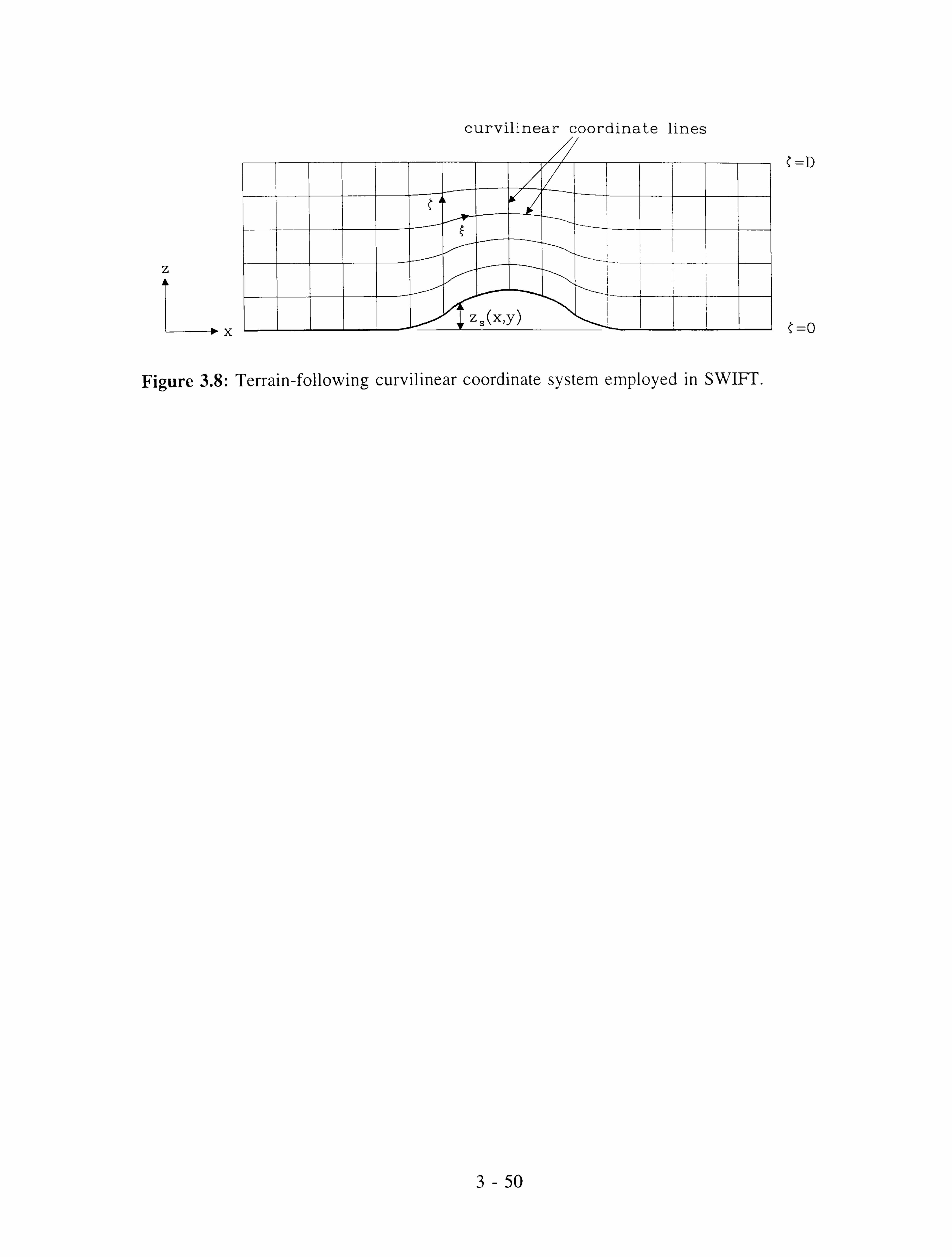
curvilinear coordinate lines

Z

Figure 3.8: Terrain-following curvilinear coordinate system employed in SWIFT.

blockage boundary

scalar cell faces and normal velocity nodes

coincide with boundary control volumes tagged as "blocked"

Figure 3.9: Arrangement of control volumes and tagged cells in bluff-body calculations.

scalar

flux specified

stress specified

tangential velocity

normal velocity

zero normal velocity

Figure 3.10: Disposition and special treatment of control volumes abutting internal boundary.

imbedded analytic domain

computational mesh

point source 44/ Z, 'X',

,. ý. _. I

/ ý

_ý ý

7

,_ ý_

Figure 3.11: Imbedded analytical region for point source calculations.

CHAPTER 4.

Turbulence Modelling

4.1 A Hierarchy of Turbulence Models

For many pressure-dominated flows a comparatively simple turbulence model suffices if one

requires only the mean field and pressure force coefficients. For example, linearised models

of flow over low hills (Jackson and Hunt, 1975; Taylor et al., 1983) have achieved

remarkably high mileage from a mixing-length description of turbulence in the inner layer,

whilst Euler flow calculations are regularly used for airfoil sections. By contrast, major

impetus for improving turbulence models has come from areas where the turbulent transport

of a scalar is of paramount importance - for example, heat transfer and pollution dispersion.

Direct numerical simulation of turbulence is not an option for any but the lowest Reynolds

number flows, although it has recently come to be used for the testing and calibrating of

various models and revealing the nature of, for example, near-wall turbulence and laminar-to-

turbulent flow transition. For most applications the choice of turbulence models lies

somewhere in the hierarchy depicted in Figure 4.1, with a preponderance of activity at the

second-order closure and (one- or two-equation) eddy-viscosity levels. In principle, the more

elevated position in the hierarchy the more general the turbulence model, but, since each step

on the ladder demands substantially greater computational effort, there comes a point where

the increase in cost exceeds available resources or outweighs any potential benefits arising

from an increase in accuracy or generality. The computational effort required for

geometrically complex three-dimensional flows is sufficiently large for us to concentrate our

efforts on tailoring simpler eddy-viscosity models to the particular flows of interest and

Sections below will describe modifications to the standard k-c model to accommodate effects

of mean-streamline curvature, alongwind pressure gradients and, in the next Chapter, a

limiting length scale. However, to set the scene and to highlight effects which are not

amenable to treatment with an isotropic eddy-viscosity model we shall first review more

general statistical closures.

4.1.1 Second-Order Closure

Second-order closure is rapidly becoming accepted as the frontline regiment in the regular

army of turbulence models (Hanjalic, 1994) to the extent that the UMIST "basic model"

(Launder, 1989) has become established as a standard framework in the same way as the

Launder and Spalding (1974) k-c model for two-equation eddy-viscosity models. In second-

order closure transport equations are solved for the individual turbulent fluxes of momentum,

uüT, and scalars, 0, which appear in the mean-flow equations. To define notation and

identify processes, the (exact) transport equations for these fluxes, together with the turbulent

kinetic energy, k=1/2q =1/2u ü, and scalar fluctuations, F, are set out below.

v cti n Mduction pressure -strain

diffusion dissipation

mean shear

body forces

D_/ir (-1-au ji c7Ut r ir

Dt \u`uý) _ CJx

+ujukax +v`uý+f u; )

kk

py Fy

Dt (ýq 2) _ ,, -iaU; , -ý +fiUi -Ui Uý-1'"

ý

vAJ

P

DD t ýeluiý) -(6ýuý

ýU` +uiujý )

lI

Pea «+ Fce>eý

6/u` Dt 2 äx t

Pe

F

ýji 'e' Fei

+Rý au, '+au;

+a p axi axt axk

0y

+piaoi p axi

0 ei

Dej

au / au/ ý

-2v `/

azk axk

Ey

I r7rt ' ý -v -

aX,

/2

ax,

E

' c3uý _(V +K)

axi aXý

Eei

ýz ýl -K( oke/ axjl"-axf "2 -- , 2- --, J I 13xi ) L

De Ee

At second-order closure level the advection and production terms are exact, but the pressure-

strain, diffusion and dissipation terms must be modelled. Turbulent fluxes derive their energy

from the mean flow (and body forces) via the production terms and lose it ultimately to heat

via viscous dissipation. Between source and sink the stresses may be advected, diffused and

-p (lL=/Öýk+UýBýý+V

a (UjUýý-UilllUk

P (ýXk

Dy

+a -p ui

+va (lgz)- 1g2u ax; p azi 22

D

a Ps '' au' a +ve/` +KLý; ý 'u, äX; Pý aX; az; +-i -

+- K-ý-v J--v ui ax, axf 22 a I__a , 1&2, loa.. I

4-2

the energy redistributed between components, mainly by the action of pressure forces in the

pressure-strain or "return-to-isotropy" term. To explain this appellation, observe that the

pressure-strain contributions for the normal stresses rte, v, ti7 are 2pu2p rý p ww Pax ýPavv

and 2P az respectively. These sum to zero (by continuity) and it is generally accepted that

their action is to attempt to bring about an equipartition of energy amongst the individual

components. The modelling of the pressure-strain interaction is crucial to second-order closure

schemes.

The divergence of the Navier-Stokes equation yields a Poisson equation for the pressure. Given the velocity field, this may be solved by standard methods to obtain the pressure field

as a sum of a volume integral over the flow domain plus a surface integral over its boundary.

Extracting the fluctuating part, it can be shown (Launder, 1989) that the pressure-strain may be written as a sum of:

(i) a term involving products of the turbulent fluctuations only;

(ii) a term containing products of Reynolds stresses and mean-velocity gradients;

(iii) a term involving body forces.

Each term is further subdivided into a volume integral plus a surface integral determining the

effect of boundaries. Given this decomposition, and the assumption that the pressure-strain

promotes a return to isotropy, a typical expression for the pressure-strain has the following

form:

i. ý ýu) ýzP) +ý

ýF) + (D; waln

!

where

(u) Eii# ýýi = -C1k(ui uJ)

-C2Pýi

(Diý = -C F. *

(walp _

[Cl ý ukul +C 2ýý +C3ýý jnk(s

iýn1 _2 ailnj _2 bý[n=)flý )

(C1=1.8, C2=C3=0.6, CI =0.5, C2=0.3, C3 =0)

(4.1)

(4.2)

and a superscript * denotes the deviatoric (ie, traceless) part: T. . =TY. -L Tkkbij. In the wall term, 11 1E is the dissipation length and 1, the normal distance from the wall. A similar form is

projected for the "pressure-scrambling" terms in the scalar-flux equations:

where

(u) ID ei

(p) ýei

(F) (D

(F)

(D cu>

+ (D (p) +A (waU)

8i _ ei ei (D ei +ý ei

-Co, E 6ýu=i k

cý -Ce2Pie

-Ce3Fe

(Deiar4 [Ceike/uý +Ce2ýýä +Ce3ýie ]nýn f( Kr )

(Cei =2.9, Ce2 =Ce3 =0.4, Cei =0.25, CA2 =Ce3 =0)

For the calibration of the various constants one is referred to Launder's paper.

(4.3)

(4.4)

The "wall" part of the pressure-strain contains the distance to the wall, in, and it is the

difficulty of specifying this normal distance for corrugated or otherwise complex boundaries

which has resulted in much recent work to reformulate the pressure-strain model in such a

way as to remove this troublesome term. Advances in this direction, together with attempts

to satisfy, for example, realisability (in particular, the positivity of normal stresses) and the

two-dimensional limit (which is approached near a wall), have been described in Launder

(1989).

The remaining terms to be parameterised are the diffusion and dissipation parts. As can be

seen from the stress-transport equations, the first typically comprises pressure diffusion,

(molecular) gradient diffusion and third-order correlations. These may be modelled

independently (Hanjalic, 1994). The dissipation term represents the ultimate sink of turbulent

energy and is usually assumed isotropic:

2 (4.5) iý _ ESýý , Eei =O

3

1/2 T/ E

If, in addition, we assume the ratio of turbulent timescales, R= k/E

0 " to be unity, then the

system of equations is closed by the specification of E. This may be accomplished either directly through a modelled transport equation, or via a dissipation length lE such that

3

E (4.6) = u° l E

where uo is a typical velocity-fluctuation magnitude. lE may be specified directly on

geometrical grounds or derived from a transport equation (eg, Mellor and Yamada, 1982).

Most of the common parameterisations involved in second-order closure tacitly assume that

all length scales are proportional to the dissipation length. An example demonstrating that this

proportionality does not hold in general is given in Chapter 5.

The principal advantage of second-order closure is its capacity to deal with strong anisotropy,

where individual stress components are selectively enhanced. This may be ascribed to the fact

that the production terms are exact and do not need modelling. Anisotropic forcing is of

particular importance in flows with body forces. Two examples arise in the atmospheric

context - buoyancy and Coriolis forces.

For buoyancy forces driven by variations in a non-passive scalar 0 we have (with gravitational

acceleration g in the negative z direction):

Ji - si3 ag6/si3

Pa

where a=-1 aP is the coefficient of expansion. Hence P cab n I

f uj' = age/uj/bi3 3 f/ 6' = ag6RSi3

(4.7)

(4.8)

Thus, buoyancy forces inject turbulence energy selectively into (or remove energy from) the

vertical velocity fluctuations and vertical scalar flux Tw.

A similar anisotropic forcing occurs in a rotating frame where there are fluctuating Coriolis

forces

4-5

�+ -2Ei[mQlum

so that, with 6 aligned with the z axis),

f/ u/ //

= 2SZEim3umuj ý l ý=0 fui

(4.9)

(4.10)

Thus, there are equal and opposite contributions 4SZü v' and -4S2ä v' to the cr' andv budgets respectively - an effect which cannot be predicted with an isotropic eddy-viscosity

model, since the net contribution to the turbulent kinetic energy is zero.

In complex three-dimensional flows, second-order closure models are expensive - transport

equations for six stress components, three scalar fluxes (per variable), dissipation E and scalar fluctuations. Various rational attempts to simplify them have been proposed - for example,

the hierarchy of turbulence models for geophysical flow problems of Mellor and Yamada

(1974,1982), based on classifying terms according to their degree of anisotropy, and the

partly related route of algebraic stress modelling, to which we shall now turn.

4.1.2 Algebraic Stress Models

Algebraic stress models represent an attempt to reduce the computational effort of full second-

order closure whilst retaining the effects of anisotropic forcing. They are based on the premise

that the rate of change of the structure function uu r/k is considerably less than that of the

turbulent kinetic energy itself; that is:

D -diff u ýu U`/u' (D u

-diff k=` uj

(P+F-E) Dt `jk Em k

(4.11)

(where "diff' stands for the diffusion term). With this simplification, the full Reynolds-stress

equations (excluding, for simplicity, the wall terms in the pressure-strain, (4.1)) reduce to the

algebraic equations

ii ui ui -? 5.. = k3 `' Eý `' 3 ='

where

y=ý-1 E

(4.1-1)

(4.13)

Here, I1,, -P; ý+F; ý is the total production term. Dissipation is taken to be isotropic: We

have assumed that C2=C3 and it is also common to assume local equilibrium (y=0). Neither

assumption is strictly necessary.

A similar simplification may be postulated for the scalar fluxes:

D -diff

6 u; /

D -diff k(j/62) II-E

+1'e-Ee (4.14) Dt

k(l/262) Dt k 1/20/2

Substitution into the transport equations yields

where

4T

(tT

1-C2

C 1 +Y

eiui - (bTkpee) + 4) ý(Peý + Gei) EE

11 Col +Ye

Ye -2

= (1 _Ce24T

(4.15)

P II_1 +1 a-1

ER E8 (4.16)

R is the ratio of turbulent timescales. Again, we have assumed C02=Ce3, whilst it is common

to assume local equilibrium (ye=0).

Equations (4.12) and (4.15) relate the turbulent fluxes to the production terms in such a way

as to retain the local anisotropy of forcing (as expressed through the production terms) but

without the history of anisotropy (as expressed by the advection terms). Thus, in a rather

simplistic fashion we can summarise the various levels of modelling in Table 4.1 below.

ý (n;; -2B;; II)

4-7

Anisotropy of forcing History of anisotropy

Reynolds-stress model Yes Yes

Algebraic stress model Yes No

Eddy-viscosity model No No

Table 4.1: Handling of anisotropy in various turbulence model closures.

At first sight, replacing six stress-transport equations by a single transport equation for k, plus

algebraic relations for the structure functions a uJ/k, might be perceived as an excellent

means of incorporating anisotropic processes without substantial cost. At the bottom line,

however, one still requires storage space and matrix solution algorithms for the uTý, so that

we have discarded the generality of second-order closure without gaining much in return. As

an additional warning, neither the conventional pressure-strain formulation in the full

Reynolds-stress closure, nor the algebraic stress equation (4.12) ensure realisability; in

particular, that each normal stress be positive.

Examination of the Table above might prompt one to wonder if eddy-viscosity models can

have any part to play in flows where anisotropy is known to assume a major role. The answer

is a resounding "yes" and the reason is simple: in many flows only one component of the

stress may be significant. This is particularly true if we are only interested in the mean flow.

If an eddy-viscosity model can be tailored to yield satisfactory values for this stress term in

the regions of the flow where it is significant then we have a useful model. Although

apparently little used in their own right, algebraic stress models have been found very useful

in indicating modifications to simpler models (such as k-c) to accommodate anisotropic

processes such as buoyancy (Gibson and Launder, 1976; Rodi, 1985) and mean-streamline

curvature (Leschziner and Rodi, 1981).

4.1.3 Eddy-Viscosity Models

By analogy with the molecular-viscosity law for Newtonian fluids. eddy-viscosity models

assume a linear relation between the (deviatoric) turbulent stress tensor and the mean rate of

strain via a (kinematic) eddy viscosity, vt:

aU. au. tij = -(u(ýuj -? kS. ) = yr (4.17)

3 ax axt

and between the turbulent scalar fluxes and mean gradients via a turbulent Prandtl number. 6e:

_6/ui

Eddy viscosity specified directly. For example, in the atmospheric surface layer (see

Section 5.2):

Vt aO ße axl

As with any other diffusivity, the eddy viscosity has dimensions of [velocity]x[length], and

this motivates its modelling. Physically, the velocity scale, 11o, should be proportional to the

magnitude of the turbulent perturbation, whilst the length scale, 1,,,, is representative of the

distance a fluid particle may move whilst retaining its dynamical properties. The four

commonest forms of model are as follows (simplest first).

(i)

xu *z 4)M(ZlLMO)

(4.18)

(4.19)

where u* is the friction velocity, LMO is the Monin-Obukhov length and 4,,, is a

stability-dependent function taking a value of unity in uniform density flow. (These

variables will be defined more precisely in Chapter 5. )

(ii) Mixing-length models. The velocity scale is taken as the change in mean velocity over

of-strain tensor. The turbulent stress is given by

a (specified) mixing length, l, n;

ie, uo=lmau , or, in a tensorially invariant form, az 1 au. au,

uo=lS, where S= 2Sý. Sý is the mean-strain invariant and Sýý=- + is the rate- 2 ax ax1

4-9

-(u1/ uj /- 32 kS1j) = 21 nSS1ý

which reduces, in a simple shear flow, to

-u/w/ = l2 m au az

au az

(4.20)

(4.21)

(iii) One-equation models. Typically, vrock'121,,,, where the length scale is specified

algebraically (usually on geometric grounds) and a transport equation is solved for the

turbulent kinetic energy k. In the atmospheric boundary layer, for example,

1 _11 --+ 1m KZ lM

(4.22)

where Kz is the eddy size determined by the distance from the surface and 1,,,.,. is some

maximum mixing length, determined, for example, by stratification or the depth of the

boundary layer. The transport equation for k will be given below.

(iv) Two-equation models. Typically, transport equations for the turbulent kinetic energy

k and either a length scale or a derived scale. In the widely used k-E turbulence model

the second transport equation is that for the dissipation rate e and we have:

velocity scale: u=C 1/4k 1/2

0µ

length scale: lm = le

giving an eddy viscosity

V. - k2

C- Iµ E

3 uo E

(4.23)

(4.24)

(The separation of constants between velocity and length scales is somewhat arbitrary:

the above choice is made for reasons of consistency. ) Note that there is only one

length scale. Modelled transport equations are solved for k and e:

4-10

Dk =a (v +vt)

ak Dt a, ý- ak aý, DE avt aE (v +)- Dt aý QE axi

+ II -E

(425)

+ (CElII CE2E)

-aQ

T E

k E

where II is the overall production rate of turbulent kinetic energy, the sum of terms

P and F due to shear and (in this application) buoyancy forces respectively:

, , av1 av; av aUý P= -uiuj = vt + a; a; axz a;

F= agw'61

1 ti

E

Vý ÖO vQe az

(4 26)

Unless specified otherwise the applications described in this Thesis use the constants

Cµ=0.097 CE1=1.44, CE2=1.92, ak=1.0, aE=1.11, ae=0.9 (4.27)

With the exception of 6E these are the values recommended by Launder and Spalding

(1974). ß£ was chosen to make the model consistent with the constant-flux, surface-

layer similarity profiles characterised by a logarithmic velocity profile (in uniform

density flow):

CEz -l. El

K2

QE Cµ (4.28)

The model is most sensitive to Cµ, which sets the general level of turbulence, and the

difference CE2-CE,, since this determines the balance of production and removal terms

in the dissipation equation and hence the length scale. In principle, C. can be

determined from the structure constant ('r/k)2, which implies C, =0.033 for rough-wall

boundary layers (Raithby et al., 1987). We have retained the more conventional value

C, =0.09, based on Klebanoff's original smooth-walled flat-plate data, since the set of

constants were originally optimised in toto and changes in C, should not be

undertaken without re-optimising CE, and CE2.

a; t( a; axz )a;

4-11

4.2 Modifications to the Standard k- e Model

Hanjalic (1994) and others have identified major deficiencies of two-equation eddy-viscosity

models. They include the inability of a linear stress-strain relationship based upon a single isotropic eddy viscosity to cope with, for example:

" history of anisotropy; eg, wake flows;

" anisotropic body forces; eg buoyancy, Coriolis forces;

" complex strains; eg, curved flows, alongwind pressure gradients;

" viscous effects in low-Reynolds-number and transitional flows;

" non-equilibrium flow near walls;

" flows with more than one length or time scale.

Whilst second-order closure can overcome the first three problems, the latter three still remain

and the modelling of the pressure-strain interaction creates new difficulties. Numerically,

Reynolds-stress transport models are computationally intensive and notoriously unstable. By

contrast, eddy-viscosity models are readily incorporated into existing laminar viscous codes

through a stability-enhancing addition to the implicit diffusion term. There is, therefore,

widespread appeal for the idea of "tweaking" eddy-viscosity models for particular types of

flow.

This Section will review briefly two particular types of extended two-equation closures - low-

Reynolds-number and non-linear k-E models - and then examine, in some detail, two k-c

modifications which have been coded in SWIFT to account for complex strains - mean-

streamline curvature and streamwie pressure gradients. In Chapter 5a novel "limited-length-

scale k-c model" is proposed for flows where the turbulent mixing length is limited by some

external constraint.

4.2.1 Low-Reynolds-Number k-c Models

Numerical practices for modelling turbulent shear flows near walls divide sharply into two

camps - low-Reynolds-number turbulence models designed to resolve the flow right down to

4-12

the viscosity-dominated sublayer and wall-function approaches which bridge the `gap between

a node lying in the fully turbulent region and the wall with some ývell-defined universal

profiles. Since atmospheric flows are inherently of high Reynolds number (and the surface is aerodynamically rough) the wall-function approach is invariably used for such simulations

and this technique will be described in Section 4.3. However, for code validation against

small-scale flows in the laboratory, integration right to the wall using a low-Reynolds-number

model may be desirable.

The requirement for an accurate prediction of flow separation and laminar/turbulent transition

means that near-wall modelling is important in many engineering flows. However, the

overriding importance of the near-wall region in thermal diffusion has inevitably meant that

much of the impetus for refining both modelling practices has come from the heat-transfer

research community. Indeed, it was the difficulty of obtaining direct experimental

measurements in the vicinity of the wall that led Chieng and Launder (1980) to suggest that

heat-transfer comparisons were perhaps the best means of assessing the near-wall modelling

of turbulence. This has all changed with the availability of detailed direct numerical

simulation (DNS) data (eg, Rodi, 1993) and it is inevitable that much more model calibration

will be carried out in future through this medium.

A large number of low-Reynolds-number k-£ models appear in the literature. A representative

sample consists of the models of Launder and Sharma (1974), Lam and Bremhorst (1981),

Chien (1982) and Lien and Leschziner (1993). Other examples can be found in the review of

Patel et al. (1985) and the work of Rodi and Mansour (1993). A common formulation for

such models has been given by Patel et al. (1985). The direct effects of molecular viscosity

on the shear stress and turbulent length scale are incorporated by the inclusion of damping

factors in the eddy-viscosity formulation and the dissipation equation; thus:

k2 Vt= C__fµ

DE =öv ýý +ýýE+ (CEiP -

CEý2E)

k+E Dt aý ßE aý

(4.9)

(4.30)

4-13

Some models (eg, Launder and Sharma, 1974, and Chien, 1982) choose to solve for the dissipation variable

E=E-D (4. ' ) 1)

where D asymptotes to the correct value of dissipation as the wall is approached (E--2vk/I� , kal�

- see Patel et al., 1985), in order to apply the convenient numerical boundary conditions=0

at the surface. f,,, f, and f, are, typically, functions of the non-dimensional combinations

l+ n u rln

V

ý "' In

V

Rr k2 VE

(4.3? )

where 1, is the normal distance from the wall. The damping factors, plus the additional terms

D and E, are given for the four representative low-Reynolds-number models in Table 4.?.

For the practical motivation behind each model one should refer to the original papers, but,

in general, f2 is chosen to reflect the change with Reynolds number of the exponent in the

decay law of isotropic turbulence, f, or E to return the correct behaviour of dissipation near

the wall, and fµ to incorporate the transition from turbulent to viscous momentum transport

as the wall is approached. Note that Lien and Leschziner's model is an attempt to effect a

smooth transition from the two-equation k-E model to a one-equation model (1,,, and 1E

specified) in the viscous sublayer.

To resolve the viscous sublayer the nearest grid node must be at an l� value of order unity.

Model fµ f1 f2 D E

Launder and Sharma

_ 3.4

e ('+8/50)2

1 1-0.3e -R' 2v ak /Z

2vß tU' Z

ax a oXk (1974)

Lam and (1 -e -0.0165C)2 Bremhorst

X (1+ 20.5 1+0.05 1 -e -R, ' 0 0 R fµ

(1981) t

Chien (1982) 1-e -0.01151 1 1-0.22e -(Rý6'2 2vk

-2v Ee -0.518

I n In

Lien and cl> clý lM IlE - C3/ak3n E

Leschziner Kln(I -e -0.01618) 1 1-0.3e -R` 0

Yµ CE 2 i' k

(1993) -0.2631, Kln(1 -e )

-1,; z/a50

xe

Table 4.2: Coefficients for low-Reynolds-number models. Note: Chien uses non-standard k-£ constants CE, =1.35, Ce2=1.8.

4.2.2 Non-Linear k-E Models

For thin shear layers, the standard k-c model works well because the normal Reynolds stresses

do not enter into the calculation of the mean velocity. Whilst this provides an acceptable

representation of the mean flow the same cannot be said for the turbulence statistics. For

example, in fully-developed channel flow the standard k-e model (or, indeed, any other

isotropic eddy-viscosity model) predicts that the normal stresses are all equal (to 2k/3), in

flagrant contradiction of experiment. As Speziale (1987) demonstrates for fully-developed

flow in non-circular ducts, in the absence of any distinction between the normal stresses, an

isotropic eddy-viscosity model will fail to predict the development of the secondary (cross-

4-15

stream) circulations which are observed in experiments. It is clear that an accurate representation of the normal stresses will be equally important in curved and separated flo%ý,,.

The search for a better representation of the normal Reynolds stresses without a sacrifice of the beneficial aspects of the k-£ model - such as its ease of application and its reduction to

a mixing-length model for thin shear flows - has prompted the development of a number of

non-linear or anisotropic extensions. Both appellations are widely used and equally

appropriate. The anisotropic property indicates an advance over the strict proportionality between deviatoric stress and mean strain. The non-linear description refers to the derivation

of models as terms in an asymptotic expansion in powers of the mean-velocity gradients, with

the standard isotropic form being obtained as the linear term (Speziale, 1991). However, a

modicum of caution needs to be exercised with this formal derivation, since the dimensionless

expansion parameter is, effectively, C. kS (S a representative velocity gradient), which takes

C the rather moderate value 0.3 in equilibrium shear flows.

Speziale (1987) derived a model based on "material frame indifference"; that is, invariance

under arbitrary (even accelerated) changes of reference frame - not just inertial

transformations. (This has been criticised as too restrictive for general turbulent flow, since

it only applies in the limit of two-dimensional turbulence and generally imposes a stronger

constraint than is satisfied by the equations of motion themselves. ) Speziale notes that terms

which are quadratic in aU; /ax1 are of the same dimension as those which are linear in

0 D/Dt(aU; /ax), whilst the frame-indifferent parts of these tensors are S1 and 5iß, where

. DS Y au` S

aU' .S3 S.. _-. Dt aXk kj - aXk In

is the Oldroyd derivative. Thus, a material-frame-indifferent model which is quadratic in the

velocity gradients (and contains the standard, isotropic, eddy-viscosity model as the linear

term) must take the form

(4.34)

where, as before, the superscript * denotes the deviatoric or traceless part. The constants cD

and cE are calibrated with respect to measurements of the normal stresses in full-developed

channel flow (where, incidentally, the advective parts Ü. VSj of the Oldroyd derivative

vanish). Values CD CE= 1.68 are adopted. Although Speziale shows (in principle) that his model

is capable of predicting secondary flows in non-circular ducts, this is not unique to his

scheme, but is generally true of non-linear models which are quadratic in the mean-velocity

gradients.

Rubinstein and Barton (1990) describe an alternative non-linear model by extending Yakhot

and Orszag's (1986) renormalisation-group (RNG) procedure, curtailing the iterative process

at second order. The often-quoted advantages claimed for the RNG analysis are that all model

constants emerge naturally from the theory rather than having to be calibrated, and that the

theory is valid for both high and low Reynolds numbers. Rubinstein and Barton's model for

the Reynolds stresses is

ii uiuj 2k -3 Sýý = 2C

(E where

au. au. +c c.

auk

+cc3avk auk ja

Iu auk au

dXk dXk ldXk dX dXk dXi ) C1Xl aX ,

Cµ =0.0845 , CT 1=0.034 ,

Cr2 =0.104 , C73 =-0.014

(4.35) *

(4.36)

Shih et al. (1993) derived a third non-linear relationship between Reynolds stress and mean

strain by considering the most general tensorially invariant combination of second order in

the mean-velocity gradients, subject to the constraints of symmetry and realisabilitiy. The latter

condition means, in particular, that the model must always return non-negative normal

stresses, u', -, and requires that the model coefficients be functions of the mean strain. or, in I- fi

ll

dimensionless form, The remaining coefficients were calibrated with respect to E ax.

rotating homogeneous shear flow and backstep flow. Shih's model takes a form very similar

to that of Rubinstein and Barton (4.35), but with coefficients which are functions of the stress

4-17

invariants:

where

Ii

S= 2SýýSzý ,0 = 2S2ýýS2ýý ,

1 aUi _aU 'j 2ai axi

S=S k0 =S2

EE

(4.38)

We turn now to two complex-strain variants of the k-c model which have been investigated

using SWIFT - variants to incorporate mean-streamline curvature and streamwise pressure

gradients. Respectively, these embody the two main ways of modifying the standard model:

(i)

(ii)

0.667 _

13 C -4 C` -2 µ_ ý3=

(-ý. 37 ) 1.25+5+0.952 tii 1000+5 -c2 1000+5 ' 1000+5

multiplying the eddy viscosity by an anisotropy-dependent factor;

modifying the length scale (indirectly) by altering the balance of production and

removal terms in the dissipation equation.

4.2.3 Streamline Curvature Modification

This modification was originally described by Leschziner and Rodi (1981) for two-

dimensional flows. A more formal mathematical derivation, based on a moving system of

basis vectors, allows a natural extension to three-dimensional flows.

If at some point in a flow we consider a cartesian coordinate system (x, y, z) with x locally in

the direction of the mean wind, then curvature is essentially the non-vanishing of the

derivative aV/ax (Figure 4.2). Inspection of the full Reynolds-stress transport equations shows

that this derivative makes contributions -2u "v "aV and -u a aV

to the production terms of v ax ax

and v respectively. Assuming that aU/ay has the same sign as the shear stress -v vv this

means that curvature will promote stability/reduce cross-stream fluctuations if au aV

<0 and aUaV ay ax

increase turbulence if ay ax

>O.

21 ax_ ax. 1 aUý aU -+ 2 a; axi

4-18

In other words, concave curvature (velocity increasing towards the centre of curvature) is

destabilising, whilst convex curvature (velocity decreasing toward the centre of curvature) is

stabilising (Figure 4.3). In the case of a boundary layer perturbed by a small hump the (non-

separated) flow typically goes through a sequence of concave-convex-concave curvature. Over the summit the opposing effects of convex curvature and increased shear respectively

act to reduce or enhance the crosswind fluctuations.

Moreover, the argument above suggests that the effects of curvature are determined by the 2

product au av or, non-dimensionalising with a turbulent timescale, by k au av ay ax E ayaX

Leschziner and Rodi (1981) showed, by an algebraic stress procedure, that this was indeed

the curvature-dependent term in a simple variant of the k-E model. The following is a more formal reworking of their method, which also extends it naturally to three dimensions.

Given a flow field Ü(x, t) one can define, at any point, streamwise and normal vectors es ande

respectively by

Ü

(4.39) aes

as

e =USS

-KCen

xc is the curvature; (reciprocal of the radius of curvature, Re). The directions of is ande

(see Figure 4.2) are well-defined in a curved flow if we adopt the convention that US>O, Kc>0,

although this means that in a planar flow en could be obtained from es by either a clockwise

or anticlockwise rotation through 90°.

Given some point in the flow, establish a rectangular cartesian coordinate system (x,, x, _v- )

which is locally aligned with the streamline system. Then, at that particular point,

el = es e2 = en (4.40)

e3 = el/ýe2

(Note, however, that {el, e2, e3} are constant vectors, whilst es and eý are functions of

4-19

position. ) Then

au 1 aus ax

2

au2 axl

an

-KC Us

(4.4 1)

To examine the effects of curvature alone we shall assume that these are the only non-zero

velocity derivatives at this point. Application of the algebraic stress model (4.12) -a local

model, remember - yields

u/2 = 3k(1-ýII/E) +

v2 = 3k(1-ýII/E) +

U'V'

(ýk(-2uIvý)aUS

E an

(ýk (2u /v ) K, - Uý E

4)k u 2x U- vý

aU ECs an

which, on eliminating the normal stresses, gives

-u/vt =

In other words,

where

3(D(1 _4)][I/, E) k2 aus , (02aU,

__ E an -x

1 +44)2 k 2aUS K US E an

_i k2 aU1 (3 a u2

12 9E aX2 aX l

(4.4? )

(4.43)

(4.44)

C= Cµ°

co µ= 3 ý(1(4.45)

1 +44ý2 2aUS

xCUs E an

(4.44) is the standard k-c eddy-viscosity-model expression for the proportionality between

shear stress and mean rate of strain, but with Cµ replacing C. Since it is the factor

multiplying C. 0 in (4.45) which embodies curvature effects, we shall use this expression to

E an

4-20

modify the k-E model, but for consistency we shall retain the more conventional value Cµ0=0.09, rather than that derived from the pressure-strain coefficient Q.

Note that the curvature-dependent factor can also be written

Cµ 1 Cµ0

1-4ý2 k 2aU aV E a)ý ax

(4.46)

in the local cartesian system. Thus, as argued earlier, positive and negative values of the k 2auaV

dimensionless combination -E ay aX respectively enhance or diminish cross-stream

turbulent transport of momentum. Leschziner and Rodi (1981) obtain the slightly different

expression

Cý µ

Cµ0

1+44)2(k 2 aUS +xc U xCUS E an

(4.47)

The difference may be traced to the Reynolds-stress production terms, P,. In Leschziner and

Rodi's paper these are supplemented by "pseudogeneration" terms which occur in the stress-

transport equations in (s, n) coordinates. However, these are actually part of the advection

term, arising as a consequence of coordinate rotation.

Although the curvature modification is most naturally depicted in two dimensions, definition

(4.39) allows Kc and aUjan to be evaluated in fully three-dimensional flows. es is the unit

vector in the direction of the local velocity. Since

zaes aus - (4.48) U. VU =U+U S as as

2, is simply the component of the advective acceleration (Ä=U-DU) normal to then -xcU e

0. Finally,

au au, au = e200(Ü"e1 )=s. n an aX2 1 ýa ý

where es=(s), en=(nj).

(4.49)

This streamline-curvature modification will be evaluated in Chapter 6 when we consider (neutrally stable) boundary-layer flow over a two-dimensional hill. To identify the regions of

stabilising and destabilising curvature we have plotted as an example in Figure 4.4 contours

of the curvature-dependent factor (4.45).

In a similar fashion to that used above, Gibson and Launder (1976) simplified the algebraic

stress model (4.12) and (4.15) to deduce a buoyancy extension of the k-c model for a

horizontal free-shear layer. Rodi (1985) generalised their work to thin shear layers parallel

to a plane wall or free surface. As with the curvature modification this led to a buoyancy-

dependent factor in C, and, in this case, the turbulent Prandtl number ße. The assumptions

underlying that theory - namely, unidirectional flow with velocity and density shear only

normal to the flow direction - are far too restrictive to give the model much prospect of

generality and its applications have been confined to vertical and horizontal buoyant jets. The

dynamical similarity between curved and buoyant flows has been discussed by Bradshaw

(1969).

4.2.4 Preferential Response of Dissipation to Normal Strains

Just as curvature could be identified with the non-vanishing of derivative aV/ax in a cartesian

coordinate system locally aligned with the flow, so the presence of an alongwind

acceleration/deceleration or streamwise pressure gradient is formally represented by non-zero

aUlax.

Experiments demonstrate that dissipative decay of turbulence is enhanced in regions of strong

favourable or adverse pressure gradients - for example, grid turbulence passed through a

contraction or decelerated boundary layers respectively. In the latter case, predicted dissipation

4-22

is too small, and hence turbulence levels too large, resulting in failure to predict flow

separation. Similarly, unphysical levels of turbulence are predicted upwind of bluff bodies,

particularly the favourable pressure gradient near the upwind corner, enhancing momentum transport across the separated shear layer and so leading to early reattachment.

Hanjalic and Launder (1980) concluded that streamwise strains are more effective than simple

shear in promoting transfer of energy from large to small scales, so enhancing the dissipation

rate, and proposed increasing the source term in the dissipation equation for normal strains. This idea of a preferential response of dissipation to normal strains was taken up by

Leschziner and Rodi (1981) whose model for the production term in the dissipation equation

can be invoked as an option in SWIFT:

k PE -

[CEIP

- C//Evt(25,

s)2] E (4.50)

where S,,, is the "shear strain", 1 au1 +au2 in a rectangular coordinate system aligned so ,,, 2 axe ax

that the xl-axis lies in the direction of the 11oca1 velocity vector. In three-dimensional flows

x, is not well-defined and the most appropriate direction is that of the component of DU,

normal to e1; ie, VU, -(e1 "VU1)e1.

In order that the modified dissipation equation should reduce to the standard form in a simple

shear flow (aU/av the only non-zero derivative) it is necessary that the new constants satisfy / //

C E1 -CE1 _ CE1 (4.51)

Following Leschziner and Rodi (1981) the values CEi =2.24, CE; 1 =0.8 have been used here.

This variant of the k-c model was also evaluated with respect to the Russian hill geometry

in Chapter 6 and we shall have more to say about its performance there. During the

development of SWIFT the code was used to compute flow over various canonical two-

dimensional bluff-body configurations. The effect was to reduce turbulence upwind of, and

hence the turbulent transport across, the shear layer separating from the upwind corner,

increasing the length of the recirculating flow to one more consistent with experimental

measurements. As an illustration, Figure 4.5 plots predicted contours of turbulent kinetic

4-23

energy with and without the dissipation modification in uniform, low-turbulence flow around

a blunt rectangular plate. The effect of the modification is to suppress the unphysical levels

of turbulence upstream predicted by the standard k-c model (with uniform approach flow and

highly favourable pressure gradient the boundary layer on the front face is laminar), restricting

the generation of turbulence to the separating shear layer.

4.3 Near-Wall Modelling By Wall Functions

Low-Reynolds-number modelling has by no means supplanted wall-function approaches. This

is particularly true for environmental flows where, not only is the Reynolds number very high,

but the surface is aerodynamically rough, so that detailed resolution down to the wall is

inconceivable. Instead, traditional wall-function approaches have been refined, particularly in

complex recirculating flow where the near-wall turbulence is far from equilibrium.

For equilibrium shear flows a common assumption is a universal relationship between

variables scaled on the local friction velocity u,. Thus

U+ = f(in) (4.52)

where

U + U(l

11 l+ _ n

'nut

V Ut (4.53)

In is the normal distance from the wall and r,,, -=u, is the (kinematic) wall shear stress. In the

fully turbulent layer:

U+=1 ln(El+)

whilst in the viscous sublayer:

(4.54)

U+ = l+ (4.55) n

Assuming a dimensionless height 1L+ for the viscous sublayer, matching the two profile,, at this height yields

e xly

E= l+ v

(4.56)

1ti+ is usually taken to be 11.6. For strict validity, wall-function approaches require the nearest

grid node to lie in the fully-turbulent region, typically in the range 30<l�*<150.

For rough-wall boundary layers (where individual surface elements exceed the depth of the

viscous sublayer) the logarithmic velocity profile is commonly written as

U+ = 1ln(l, Jzo) (-l. 57) K

where zo is the roughness length.

Using (4.54) or (4.57), UT (and hence t,,. ) may be deduced from the velocity value at the near-

wall node. The difficulty with scaling on the friction velocity, however, is that near stagnation

points it, (and hence the eddy viscosity v) vanish. Thus, the eddy diffusivity for heat, v/68,

also vanishes, whereas, in practice, the heat transfer coefficient exhibits a maximum at this

point. An appropriate means of overcoming this (Chieng and Launder, 1980, based on the

work of Spalding, 1967) is to use the square root of the turbulent kinetic energy, A, as a

velocity scale, rather than It.. In equilibrium flows the two formulations are equivalent since 1r4, /2 ^µ k (4.58)

However, the main advantages are perceived near stagnation points, where, unlike cat, there

is no requirement for k to go to zero.

According to Spalding (1967) the viscous sublayer thickness, 1, adjusts itself in line with the

external kinetic energy so that the sublayer Reynolds number, l, ̀ -l,, k, '/Z/v, is a universal

constant with a value of --20 (Launder, 1988).

In the fully turbulent layer assume an eddy-viscosity relationship for the shear stress: aU

'Lw =V `än

where, by comparison with the equilibrium case, the eddy viscosity is given by

vt = x(Cµ4k'ý2)ln

Integrating for the velocity profile (with constant k and yields

Cv4kh/2U 1 -1n(E 1, )

t w K

where In*=lnk''Z/v and, for consistency with the equilibrium case, E'=C, E.

(4.59)

(4.60)

(4.61)

The value of k appearing in (4.61) is kv, the turbulent kinetic energy at the top of the viscous

sublayer. Although various means have been devised to obtain this by extrapolation (eg,

Chieng and Launder, 1980), the value kp at the nearest internal node is almost always used.

With the tangential velocity component Up at the same location, (4.61) can be inverted to

yield the wall shear stress

xC. '. /°k'/2 U_ 'C =

w ln(E * lp )

(4.62)

Numerically, this shear stress acting on the face of a control volume abutting the wall may

be included explicitly (as a source term) or implicitly, via an effective eddy viscosity vt, eff such

that

U_ tiw = vt, eff ll

P

-P

µNp

(4.63)

where

KCµ`kp2 1

ýreff ln(E*lp)

(4.64)

A comparable treatment is available for the heat flux (Launder, 1988). but within SWIFT we

have adopted the simplest procedure of using vt, fj,

66 as an effective eddy diffusivity.

For rough-wall boundary layers an exactly similar procedure is followed, except thatE 'IP

is replaced in the logarithmic term by ln/zo.

For equilibrium boundary layers, k is related to in by (4.58) and, if i is deduced from the

velocity profile above, then this serves as a boundary condition to specify the near-wall value

of k. For flows departing from equilibrium, however, it is the near-wall value of k that

supplies the velocity scale and a more accurate balance of production and dissipation within

the near-wall control volume is sought. Cell-averaged values of production and dissipation

are obtained from specified profiles of U, k, e and 'z over the depth of the near-wall cell.

Idealised profiles are suggested by Figure 4.6.

In the viscous sublayer, experiments suggest a linear variation in the amplitude of the

fluctuating velocity component parallel to the wall, which leads to a quadratic variation in k:

2

k= kv l

1n (4.65)

V

As the wall is approached the diffusion of turbulent kinetic energy occurs by molecular

gradient transport, which, according to this profile, vanishes at the surface. The appropriate

numerical boundary condition is, therefore, no diffusion through this face.

In the viscous sublayer E tends to a constant value c,. (Patel et al., 1985) where

2vk v E_

v2 lV

whilst in the fully turbulent layer, where dissipation balances production:

(4.66)

4-27

C 3/4k 3/2

E/lI nl

=µ \

KI n

(4.67)

The cell-averaged value of F_ is, therefore, (assuming k, =k,, ):

10lC 3/4k 3/2

E= -f E dl =Ev+µP 1n(0/l) (4-68)

00nv0 KA v

The turbulent kinetic energy production rate is given by

an ln'l

p=n

0l <l nv

and hence the cell-averaged value is

2

P= 1 JýP dl =

iW 1n(0/1 ) A0n

Cµ4kp2Ko

(4.69)

(4.70)

Equations (4.68) and (4.70) require amendment for rough-wall boundary layers where there

is no viscous sublayer and the formal integration is carried out down to In this case.

C 3/4k 3/2

E=µp ln(l, t/lo) KO

2 Tw

ln(l,. t/lo) Cµs%Cp ZKO

(4.7H

direct numerical simulation

higher-order closure

Reynolds-stress transport model

eddy-viscosity model

mixing-length model

algebraic stress model

two-equation model; eg, k-epsilon

one-equation model; eg, k or I

one-equation model; eddy viscosity specified

Figure 4.1: Hierarchy of turbulence models.

local system of basis vectors

Figure 4.2: Local system of basis vectors for curved flows.

stable curvature unstable curvature

Figure 4.3: Stable and unstable curvature for boundary-layer flow.

Figure 4.4: Regions of stable and unstable curvature in shear flow over a hump. Contours demark areas where the curvature-dependent factor in the eddy-viscosity expression departs from unity by more than 30%.

U

-P to b

-W W -W 01

uniform approach flow

LH

blunt rectangular plate

(a) Standard k-c model

(b) With dissipation modification

Figure 4.5: Computed contours of turbulent kinetic energy (k/U02) for flow around a blunt

rectangular plate. The dashed line shows the separation streamline.

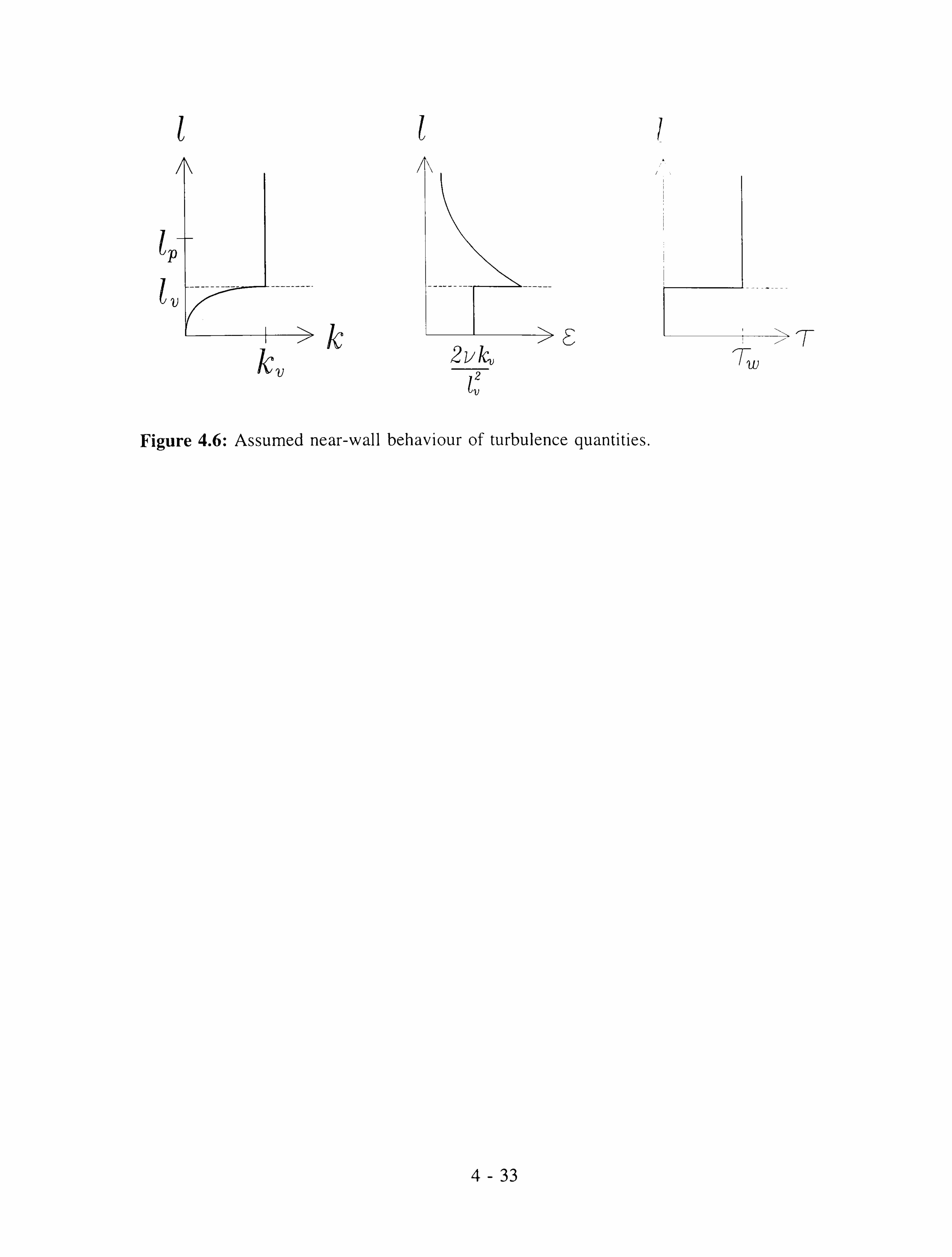
1 /ý\ /T\

Ip

IV ----------- ---------

kv ý i I>F,

2vk� lz v

Figure 4.6: Assumed near-wall behaviour of turbulence quantities.

CHAPTER 5.

Atmospheric Boundary-Layer Modelling

Turbulent shear flows arise in many areas of fluid mechanics. In most instances they are limited in physical extent and in numbers of people affected. However, one deep turbulent

shear flow - the atmospheric boundary layer - impinges upon us all and it seems worthwhile, if not imperative, to make an effort to understand and model it.

Dynamically, however, the atmospheric boundary layer (ABL) is far more complex than most "engineering" flows for it involves:

" temporal and spatial variation;

" buoyancy forces;

" Coriolis forces.

For this reason we should not expect turbulence models designed and calibrated in

engineering laboratories to work well without modification in atmospheric flows. Nor are

alternative models easy to validate: the depth of the ABL, typically between 100 and 2000m,

makes it less amenable to experimental measurement than boundary-layer flows of more

limited extent.

Coriolis forces arise from fluid motions observed on a rotating reference frame called the

earth. They lead to the large circulatory systems around pressure "highs" and "lows" on our

weather maps. Locally, they lead to a turning of the wind with height.

The density differences responsible for buoyancy forces arise from differential heating and

cooling. On a hot day the ground and the air next to it are heated by solar radiation, driving

convection and generating a deep, well-mixed, turbulent layer. In the absence of an external

source of heat at night the ground cools by radiation and a stably stratified layer develops.

Buoyancy forces then inhibit vertical motions - both the mean flow around terrain undulations

and the turbulent fluctuations responsible for the cross-stream transport of heat and

momentum. Since these same fluctuations are responsible for diffusing pollutants it becomes

important to parameterise the effects of buoyancy in turbulence models.

Perhaps the hardest aspects of the ABL to model are temporal and spatial inhomogeneities.

Time-dependence of the radiation balance is forced by the diurnal and seasonal variational

of incoming solar radiation (which is predictable) and is complicated by latent heat transport

and the evolution of clouds (which is not - much). Spatial inhomogeneities may arise from

variations in surface properties (for example, elevation, roughness, albedo and water content)

and from the passage of large-scale features such as weather fronts. However, there is

evidence that, under uniform surface conditions and provided the rate of surface cooling is

not such as to eradicate turbulence, quasi-equilibrium states may be attained by the ABL

(Mason and Derbyshire, 1990) and this will be implicit in what follows.

5.1 Atmospheric Boundary-Layer Equations

Throughout this Chapter we shall consider an idealised, horizontally homogeneous.

atmospheric boundary layer (ABL) over a flat plane, wherein the mean velocity U=(U, V, O)

and potential temperature 0 are functions of the vertical coordinate alone. Since there is no

mean vertical motion the flow is in hydrostatic balance:

= -PS `�. 1, aP (5,,

az

and as density is a function of z only it follows that aZP1axaz=a2P1a1"1a,. =0, and hence that the

horizontal pressure gradients aP/ax, aP/ay are independent of height; (ie, the boundary layer

is barotropic).

5.1.1 Mean-Velocity Equations

The Navier-Stokes equations give for the horizontal components of momentum:

DU 12P Dt pax

DV 1 aP Dt päy

+ fv

fu

at + Xz az

at +y az

where (TXZ, Tyz)=( -u w, - w7) are the non-zero components of the (kinematic) shear stre"s

and j 2QsinX is the Coriolis parameter. (Q is the angular rotation rate of the earth and the

=10-4S-1 ). For large z the mean-velocity components are assumed latitude. At mid-latitudes, f

to approach constant values (UK, V, ) and the horizontal shear stresses to vanish. Under

horizontally homogeneous, steady-state conditions the advection terms disappear and the

constant pressure gradients can be written in terms of the geostrophic wind velocities

prevailing at the top of the boundary layer:

U_ lap v=

1ap 9

Pf a1' 9 Pf ax

The boundary-layer equations then reduce to

at xz = f( v- vg)

az atiyZ - q1T_TT

aZ - Jkv -v8ý

or, more conveniently, in complex variable notation:

aT =i fW_W) g aZ

where i=' l +i'L,. Z, W=U+iV.

(5.3)

(5.4)

(5.5)

Vertical profiles of U and V require a closure model for the shear stress which will be

discussed below. However, two points about the presence of Coriolis forces are worth making

here.

The first is that most numerical models of the ABL consider only a uni-directional approach

flow. However, without Coriolis forces a horizontally homogeneous boundary layer is not possible - the boundary layer must grow. (Mathematically, k/az-constall t implies that 't is

either constant or varies linearly with height - indefinitely). At the top of the boundary layer

where the stress divergence vanishes the Coriolis force must balance the applied pressure gradient. This apparently trivial point nevertheless precludes the modelling of pressure-drit, en boundary layers as uni-directional flow with periodic boundary conditions.

The second point concerns a little numerical difficulty in the iterative solution of the boundary-layer equations. If we assume for the moment that the shear stress is given by some

constant eddy viscosity v, then

aw T=V-

`az

and equation (5.5) becomes

a2W _

if ýW_W ) äz 2vt

with solutions

W-W = -We t(fl2v, )1/2(1 +i)z

(5.6)

(5.7)

(5.8)

(We have adopted the somewhat partisan assumption that f is positive; ie, we are in the

northern hemisphere. Those from down-under may replace f by LfI and l+i by 1-i). The

negative sign should be taken in the exponent to give the appropriate asymptotic limit W--- > W9

as z-oo (and the classical 45° turning of the wind over the depth of the boundary layer - Ekman, 1905). However, without a little caution it is quite possible for an iterative numerical

solution to pick up the growing exponent, leading to rapid divergence. To illustrate this,

consider the centred spatial difference form of (5.7) which can be written as

Wk-1/2(Wk+i+Wk-1) _ -*Wk-Wg) ý

fQ2

2v, (5.9)

on a regular mesh of spacing A. Now this system is tri-diagonal and hence soluble in its own

right for the complex velocity { Wk } given appropriate boundary conditions. It is satisfied, for

5-4

example, by Wk=WK. A difficulty arises, however, in the use of the finite-volume code described in Chapter 3 where the system (5.9) is solved iteratively and componentýý ise b`

alternating between U and V equations and using the most recent values for the source terms

on the RHS. A small error VkO at point ko first produces a perturbation in U of order SVko and then a perturbation in V of order -ý2Vko. (This is not the precise solution, which depends on the nature and location of the boundaries. It does, however, correctly describe the magnitude

of the perturbation. ) Sequential iteration, therefore, produces an exponentially growing instability if ý>1, which can only be prevented by placing an unsatisfactory restriction on the

mesh scale A. Relaxation helps a little, the condition for stability becoming rý<1, but this has

the disadvantage of slowing down convergence. To overcome this problem we have employed

a form of local relaxation which has little effect in the fine-mesh regions where there are high

gradients, but prevents numerical instabilities growing in the coarse-mesh regions at the top

of the boundary layer where U and V depart little from their free-stream values UK and V'.

In the complex equation (5.9) this amounts to replacing the explicit value Wk} from the

previous iteration on the RHS by the implicit Wk'-iý(Wk Wk ). The iterative version of

equation (5.9) can then be written

(1+ý2)Wk - 1/2(Wk+i+Wk-i) - -iý(Wk - g) + ýZWk (5.10)

and it can be shown that perturbations from the geostrophic solution (Wk=Wg) are reduced by

a factor of order ý<1,

stabilising the iterative solution. 1+2

5.1.2 Mean Temperature Profile and the Effect of Buoyancy Forces

Due to the diurnal cycle of solar radiation the ABL is seldom in a state of thermal

equilibrium and temperature variations occur which cause density variations and hence a

change in gravitational forces. Where there is no mean vertical motion the gravitational force

is balanced by a pressure gradient according to the hydrostatic relation (5.1). Departures from

equilibrium - in particular, turbulent fluctuations - lead to a net buoyancy force per unit mass

(P -PQ) g= ag(e -6Q) Pa

(5.11)

where subscript a denotes ambient conditions. a=-1 aP

pU is the coefficient of expansion,

... I- equal to 1IT for perfect gases. r

Buoyancy forces affect the mean-velocity profiles in two ways: directly, as a source term in

the momentum equation; and indirectly, by their effect on the turbulent shear stress. In stably

stratified flows the restoring forces brought about by the former can give rise to gravity (or

internal) wave motions. In this Chapter, however, we shall assume a horizontally

homogeneous boundary layer with no mean vertical motion. Buoyancy effects, therefore, will be confined to turbulence. In the turbulent kinetic energy equation they appear as a source

term (negative in stable conditions):

G= -g P/'"t'/

= ocg6'w' Po

The vertical heat flux is pc U77.

(s. 1? )

Now, we have postulated the existence of a steady-state stable boundary layer. But if there

is a net loss of heat to the ground with no compensating heat flux at the top of the layer then

the boundary layer as a whole must cool. We must, therefore, relax our definition somewhat.

Following Nieuwstadt (1984,1985) we define a steady-state ABL to be one in which the

turbulent fluxes (and thence, by assumption, the mean vertical gradients) are independent of

time. Both theoretical investigation and numerical studies (Derbyshire, 1990; Mason and

Derbyshire, 1990) indicate that, provided the surface cooling is not too extreme, the ABL may

indeed approach such a quasi-equilibrium state, with a relaxation time of O(f -` ). Derbyshire

demonstrates theoretically that for given synoptic parameters (surface buoyancy flux and

geostrophic wind speed) the (thermal) boundary-layer depth h cannot grow indefinitely.

Essentially this is because to maintain turbulence the integrated working of buoyancy forces

over the depth of the layer must be less than the overall production by shear stresses. which

can be bounded above by a factor involving the geostrophic wind speed and surface drag

coefficient alone.

5-6

Consider the consequences of this quasi-steady-state assumption for the (potential)

temperature equation:

w ace -- at az 0-13)

(We have ignored the small molecular component of the heat flux. ) Taking derivatives with

respect to t or z and assuming 6'w/ and a0/az are independent of time we deduce that:

(i) the boundary layer as a whole cools at a constant rate: a0/at=constant;

(ii) the heat flux varies linearly with height; ie,

6V = 6Vö(1-z/h) (5.14)

Meteorological evidence from Cabauw in the Netherlands (Nieuwstadt, 1984) lends

some support for this.

Numerically, global cooling may be incorporated within a steady-state one-dimensional

boundary-layer model by solving for the temperature difference between each field point and

a reference point; (for example, the surface). The constant cooling rate then appears as a

source term on the RHS of the potential temperature equation:

D (o -©r) =- ý'

-a (e'w) Dt at az

where, if h and U770 are supplied, a0, /at is given by

ý, I e'w, ö VC7

at r-ýh

(5.15)

z<h (5.16)

0 z>h

Since the LHS of (5.15) vanishes this gives the desired linear variation of heat flux with

height. However, the model cannot generate the inversion (temperature jump) which must, in

practice, develop at z=h to accommodate the net loss of heat from the boundary layer.

5.2 Surface-Layer Similarity Theory

The balance of Coriolis forces and stress divergence in equation (5.2) gives an estimate of the relative change in the shear stress over height A:

Dti fUgOz

2 ý0 U. (5.17)

Hence the shear stress may be regarded as essentially constant (it. ) over height Az<c9 UK/f,

where c, =u. /Ug is a surface drag coefficient. Typical values for a neutrally stable boundary

layer at mid-latitudes are cx=0.05, Ug=10m s -', f=104s', giving a height scale 250m.

A remarkably successful similarity theory has been built up for this (uni-directional) constant-

stress surface layer. For neutrally stable flows well above any rough surface undulations the

only available velocity and length scales are the friction velocity it. and height so that

zdU= constant =1 u* dz x

(5.18)

where K is a universal constant (Von Karman's constant) with a value of approximately 0.4.

This integrates immediately to give the well-known logarithmic wind profile:

U U=* 1n(z/za)

KZ

with roughness length zo depending on the nature of the surface.

(5.19)

For boundary layers subject to surface heating or cooling an additional dimensional parameter

is available: the surface heat flux QH=pcP6ý 7 or, derived from it, the buoyancy flux (for

ideal gases):

! '- -n "A 'AA

11 - gQH

v- ws v ºY

pcpT (5.20)

Again, this turbulent flux may be regarded as constant over a (somewhat shallower) surface

layer. Comparing production or removal of turbulent kinetic energy by buoyancy forces (G)

with production by shear (P--u, 3/xz) we find that there is a height scale L,,,, where the two terms are of comparable magnitude. Lv10, the Monin-Obukhov length. is given by

3

L.,., _U* (5.21) mu K(-G)

and, with this sign convention, LMO is positive or negative in stable or unstable conditions

respectively.

The presence of a second length scale means that the dimensionless combination z dU must

uY dz be a function of z1LMO. We write

uU ýM`ZI LM i

* dz K

with 0,11(0)=1 to conform to the neutral limit.

(5 22)

Arya (1982) and Pasquill and Smith (1983) list empirical and theoretical expressions for the

similarity function 4M in stable and unstable boundary layers. We shall confine attention to

the stable case for which a well-established form is

(ýM =1 +ßz/LMO ,ß =5 (5.23)

With (5.23) equation (5.22) integrates to give a log-linear profile

U=u *` [ln(z/zo) +ß zl LMO] K

which is well-attested by surface-layer data.

(5.24)

Similarity theory is not restricted to the mean velocity but may also be used to deduce

profiles for scalar variables - passive or otherwise. In this case a scale magnitude may be

determined from the vertical flux via

(5.25)

Then

6� a© -1 ýH(zILMO) Z

(ý. -16)

For potential temperature we have typically

ýH = Ut+ß z1LMO (5.27)

where 6, =0.7, (3'=5.0. and L,,, (, are related by

2 u*

KagLMO (5 28)

Before moving on to consider the boundary layer as a whole it is appropriate to make some

additional remarks which will influence the matching of surface and Ekman layers.

(i) Similarity relations (5.22) and (5.26) for the mean velocity and potential temperature

profiles are equivalent to gradient-transfer relations with height-dependent eddy diffusivities

KM = Ku *Z/4)M

KH = Ku *z/ 4>H

(5.29)

(ii) The potential temperature profile deduced from (5.26) and (5.27) is often observed to

be a good approximation far above its theoretical limit L, 10. In the limit as . /L4fo->-

the profile tends to one of uniform gradient with buoyancy frequency N given by

1/2 u N= agd© ýý* dz KL Mo

(5.30)

In addition the gradient Richardson number Ri and flux Richardson number R1 defined

by

d0 ag

Ri _ dz

Rf aS(-6 /w ý- f dÜ

(5-31)

j1 z ti . dz I dz

tend to constant values (3'/(32 and 1/ß respectively, or, roughly, 0.2-0.25 with commonly accepted values.

5.3 Local Scaling: Nieuwstadt's Model

Surface-layer theory is applicable only for z<_LMO. In moderate to high stability, where LMO/h<l, it provides a means of matching to the surface boundary conditions but says little

about mean flow profiles in the boundary layer as a whole.

Stable stratification restricts the vertical migration of fluid particles and hence the size of

turbulent eddies so that throughout most of the boundary layer h is not an appropriate length

scale and it is the local rather than surface fluxes which are relevant. The local scaling

hypothesis (Nieuwstadt, 1984) constitutes a similarity approach to stable boundary layers. It

postulates that (locally-scaled) dimensional combinations of variables can be expressed as

functions of the single parameter z/AMO, where AMO is the local Monin-Obukhov length

defined by

ti nMO

I 3/2 -u

/W / I3/2

K( -c) K«g(-e'W ) (5.32)

In the limit as z/AMO>oo dimensionless combinations must approach constant values. This is

the regime of z-less stratification. In particular, Richardson numbers Ri and Rf become

constants.

Nieuwstadt (1984,1985) derived an analytical model of the stable ABL in this constant-

Richardson-number regime. His main assumptions were

5- 11

(Al) Steady-state (in the sense of time-independent fluxes). As we have seen this leads to a heat flux varying linearly with height:

6/ w'=6'w ö(1-z/h)

(A2) Richardson numbers constant over the depth of the boundary layer; ie,

d© ag

dz = Ri, constant i,

ag(-e'w) dÜ ti. dz

dÜF dz

Rý, constant

(A3) Stress parallel to shear. Then, using complex variable notation with aci W=U+iV, we have t. _-aW and hence, from (5.33) and (5.34), az az

_B i aW

= B-° (1 -z/h)

zf

where Bo=ag(-6Tý)O=u; /lLMO is the (downward) surface buoyancy flux.

We solve (5.35) in conjunction with the momentum equation

ati = ZW_Wg) äZ

Differentiating (5.36) with respect to z and substituting in (5.35) gives

C)2 -C

az 2

This has the similarity solution

_i B°f

(i _Z/h) Rf

i=u? (1-z/h)"

where equating exponents and multiplying factors yields

(5.33)

(5.34)

T=T, ,- +1T,,,

(5.35)

(5.36)

(5.37)

(5.38)

5- 12

a+a-2 =1

a(a 1) - IBGfli' R4 .ý*

from which it follows that

and

a=3 +i ý3

(sgn . fl

22

i 5. ý91

(5. -tO)

h2 = ýRf u4*_ ýxRfu`L"'° (5. -11) Bolf If

This is readily identified with the Zilitinkevich (1989) formula for the stable boundary-layer height, h=c(1, L, t, (1J)'

2, with a constant value c=0.4.

The mean-velocity profile can now be obtained from the momentum equation:

W -W

u *

1he '3 S8n . fý

1 _Z/hýi

; +t 2

SSn . ý)

KRf LMo

In particular, since W=O on =O, this implies a geostrophic velocity magnitude Wg1

_1h

(5.42)

(5.43) UKR fLMo

and a wind direction shear of 60° over the depth of the boundary layer.

The mean potential temperature can be obtained from the assumption of constant gradient

Richardson number:

©_Oo Ri _h

In(1_Z/h) e* KRf LMo

(5.44)

Note the logarithmic singularity at the top of the boundary layer. Clearly, Nieuwstadt's model

is inadequate here, but the profile does imply a large temperature inversion at this height.

5- 13

Derbyshire (1990) has re-examined Nieuwstadt's model and lists the main criticisms levelled

at the theory: the assumption of steady-state, singularity in the temperature profile at the top

of the boundary layer, no explicit treatment of internal wave effects and the lack of

consistency outside the strong stability limit. The ageostrophic wind angle (60") is too large.

Also, from (5.41) and (5.43) we deduce

(5.45)

Thus, according to Nieuwstadt's theory, the downward surface heat flux is determined

completely by the synoptic parameter Wg I whereas, in practice, it is an independent

parameter. (In most cases the soil heat flux is comparatively small so that the sensible heat

flux in the air balances the loss of heat by radiation, which is essentially determined by cloud

cover. )

Despite these criticisms, Derbyshire (1990) goes on to identify the role of Nieuwstadt's model

as the asymptotically valid case in the strong stability limit h/L, i,,, >oo. In this case (5.45) is

identified as the maximum downward buoyancy flux.

Bo RfIW2

Vý3-

In the moderately stable or neutral case and in the surface layer the least sustainable

assumption of Nieuwstadt's model is that of constant Rf. Now, from the stress and velocity

profiles and the corresponding flux and mean profiles for temperature we can deduce gradient

transfer coefficients KM and KH for momentum and heat respectively:

KM = Ku *R/, Mo(l -zjh)2

KH R`

xu * -1 LMo(1-z/h)2 Ri

(5.46)

In an appendix to his 1985 paper Nieuwstadt proposes to match these to the surface-layer

transfer coefficients; thus, for example,

K� = xu *z(1-z/h)2

N, 1 +zlRILMo (5.47)

which has the correct asymptotic behaviour in the limits z/RfL,,, o- >- and : /RILAIO-*O.

2

5- 14

However the boundary-layer profiles cannot then be obtained in closed form and the equation must be solved numerically.

5.4 Other Atmospheric Boundary-Layer Closure Models

Holtslag and Nieuwstadt (1986) provide a useful regime diagram for the idealised

stable/neutral/unstable ABL (Figure 5.1), illustrating the scaling parameters applicable in

various regions of (z/h, h/LMO)-space .

Diffusion models for these distinct regimes have been

described by Gryning et al. (1987). In Sections 5.2 and 5.3 we reviewed analytical models

of ABL structure in two particular regimes: the constant-flux, near-surface region described

by Monin-Obukhov similarity theory and the constant-Richardson-number, local-scaling model

of Nieuwstadt. Although highly successful in their own right (particularly surface-laycr

similarity theory which often applies over the entire depth covered by ground-based

meteorological instruments), they represent the asymptotic behaviour in distinct regions of the

flow and are not easily reconcilable. The same may be said of other attempts to match models

across the boundaries in the regime diagram. To determine boundary-layer structure over the

entire height and stability range one must resort to more complex turbulence equations, which

may only be solved by numerical means.

Numerical modelling of ABL structure has been undertaken with all levels of turbulence

closure in the hierarchy described in Chapter 4. An alternative hierarchy of turbulence models

specifically for the atmospheric boundary layer has been developed over a number of years

by Mellor and Yamada (1974,1982), based on the systematic simplification of a second-

order-closure model. Sub-models of various degrees of complexity were derived by neglecting

terms of successive order in an anisotropy parameter a, where a is the magnitude (precise

definition not specified) of the anisotropy tensor

Qij = ui uj 2

k3S `ý (5.48)

The fundamental (level 4) model is essentially a second-order-closure model, solving

equations for the Reynolds stresses, scalar fluxes and scalar variances. The major difference

5-15

between this model and the Reynolds-stress transport models familiar to mechanical engineers is the use of a turbulence length scale 1 rather than turbulence dissipation rate E as a scale- determining variable. In the original paper (Mellor and Yamada, 1974) the length scale \\'as

specified algebraically:

KZ I=ý +ý1, ýý

(5.49)

Later, this prescription was replaced by a prognostic equation for the turbulence length scale (strictly for kl). Mellor and Yamada maintain that the solution of an equation for turbulence

dissipation is fundamentally unsound, but, equally, their model is incomplete, in the sense that

geometry-dependent terms must appear in the scale-determining equation to return the correct

behaviour near boundaries. The level 3 model is essentially an algebraic stress model with

transport equations for the turbulent kinetic energy but algebraic relations for the individual

Reynolds stresses. The level 2 model abandons advection and diffusion (ie, there are no

turbulence transport equations), but retains algebraic forms for the production, dissipation and

redistribution terms. Level 1 corresponds roughly to a mixing-length model. In their 1982

consolidation work, Mellor and Yamada insert an intermediate level 2'/z model, abandoning

the transport equation for the scalar fluctuations (by neglecting advection and diffusion) but

retaining the full turbulent transport equation for k. It is, perhaps, unfortunate that the models

developed by the engineering community are often distinct from those familiar to atmospheric

physicists. The widely-used k-c model, for example, has no place in Mellor and Yamada's

system.

We return now to the application of more conventional engineering-type turbulence models

to the idealised, spatially homogeneous ABL. One- and two-equation closures will be

examined in more detail in Section 5.5. In the remainder of this Section a brief review of

more complex models will be undertaken.

In a series of papers, Wyngaard et al. (1974), Wyngaard and Cote (1974) and Wyngaard

(1975) used a second-order-closure model to examine the turbulence structure of steady-state

neutral, evolving convective and evolving stable atmospheric boundary layers respectively.

Interestingly, the stable boundary-layer simulations indicated approach to a steady state

5-16

(capped by an inversion) a few hours after transition. They also revealed the process of formation of a supergeostrophic nocturnal jet: essentially an inertial oscillation as turbulent transport collapsed at the top of the boundary layer.

Beyond the realms of single-point closures, both large-eddy simulation (LES) and direct

numerical simulation (DNS) have been used to predict the structure of the atmospheric boundary layer. Both integrate the time-dependent Navier-Stokes equations. In LES the sub-

grid scales have to be parameterised. In DNS the mesh is small enough for all relevant scales

to be resolved. This means all scales from the Kolmogorov length (V/)'' to the boundary-

layer depth h, which imposes a severe restriction on accessible Reynolds numbers.

Large-eddy simulations have been performed for the neutrally stable ABL by Mason and Thomson (1987), for the convective ABL by Mason (1989) and for the stably stratified ABL

by Mason and Derbyshire (1990). In the stable case a particularly important advantage of LES

over conventional one-point closures is the ability to resolve explicitly both turbulence and

waves. Mason and Derbyshire (1990) followed the time evolution of a stable ABL subject to

constant heat flux or constant cooling rate at the lower boundary. Provided the downward heat

flux was not sufficient to eradicate turbulence, both converged to qualitatively similar final

states. This approach to a quasi-steady state is in line with the theoretical arguments of

Derbyshire (1990) and the second-order-closure model of Wyngaard (1975). The simulations

confirmed the usefulness of the local scaling concept (Nieuwstadt, 1984) and the apparently

minor role played by wave radiation in energy transport over flat terrain.

Direct numerical simulation of the Ekman boundary layer is the subject of papers by Coleman

et al. (1990) for the neutral ABL and Coleman et al. (1992) for the stably stratified ABL. In

the latter case the simulations agreed well with Mason and Derbyshire's (1990) LES studies

and once more confirmed the usefulness of the local-scaling concept. DNS profiles for the

dissipation rate £ compared favourably with the models of Brost and Wyngaard (1978)

(buoyancy length (Y�JN; velocity scale k') and Hunt et al. (1987) (shear length scale

6�1(dU/dz); velocity scale ß . ). More will be said about these models in the next Section.

5.5 A Limited-Length-Scale k-£ Model

In the vast majority of eddy-viscosity models (and many more complex models. too) it is

commonly assumed that there is only one length scale and hence that the mixing length 1,,, and

dissipation length l=uö/E are equal. That this need not be the case may be demonstrated by

the following simple argument.

Consider a stably stratified equilibrium shear flow with mean velocity U(,. ) and (kinematic)

shear stress 'r given by

dU T=V

`dz (5.50)

The eddy viscosity v, is the product of a mixing length 1,,, and velocity scale it,,. In this simple

equilibrium layer

u= l__. dU (5.51) v',. 7Z

so that, on multiplying by it,,,

2 dU uo =vt =i dz

Hence i`2 is the appropriate velocity scale. But now, by local equilibrium:

P+G =E

whilst, by the eddy-viscosity hypothesis for the shear stress,

P=eau=-C 2

az vt

(5. s2)

(5.53)

(5.54)

Hence, dividing (5.53) by (5.54) leads to

vý =E (1-Rf)

where

R= -G fP

(5.55)

(5.56)

is the flux Richardson number, the ratio of the rate of removal of turbulent kinetic energy by

buoyancy forces to its production by shear. Since the velocity scale is T", equation (5.55)

represents a relation between length scales:

lm =/ (1-Rf) (5.57)

Equation (5.55) is equivalent to the standard k-E model in neutral flow if Cp is the structure

function (, r/k)'. Here, in the absence of better data, this is assumed to be the same as in

neutral flow over the same surface, although Rodi (1987) suggests that 't/k is itself a function

of Rt.

Note that the 1-R, factor governs the ratio of mixing length to dissipation length. It is quite

distinct from the rather more stringent Richardson-number dependency exhibited in the

surface layer by the mixing length:

1= xz(1-1Rf) , ßz5 (5.58)

We now come to the central premise of this Section: that, in many flows of interest, there is

some maximum size of turbulent eddy -a scale defined, for example, by boundary-layer depth

or imposed by stratification.

This is easily incorporated into one-equation models where the mixing length is specified

algebraically: for example, in a simple shear flow:

1_1+1 1m KZ 1 rrmax

or, equivalently,

l m KZ

1 +KZ/1max

(x. 59)

(5.60)

However, the k-E model is essentially a single-length-scale model, with 1,,, identically equal to the dissipation length. In the above example the standard k-c model will give a length scale

growing approximately linearly with height.

Detering and Etling (1985), in their simulation of the Leipzig wind profile, concluded that the

standard k-c model when applied to the atmospheric boundary layer yields

"a very deep boundary layer

" large mixing length (and hence eddy viscosity) in the upper boundary layer

" large friction velocity

" small cross-isobar angle

when compared with observations. These deficiencies can all be traced to the inability of the

k-c model in its standard form to recognise some finite upper limit to the mixing length. By

contrast a one-equation (k) model, with mixing length prescribed by (5.60), compared very

favourably with experimental observations when an appropriate value of 1,,, c� was used.

There are thus two requirements of the new model: (i) to specify the maximum mixing length;

(ii) to modify the two-equation turbulence model to accommodate

Dealing first with (i), may be either a global (ie, fixed) scale, or one defined locally in

terms of, for example, mean-flow gradients. We have found the former both more practical

and more realistic. For example, in jet or wake flows l could be taken as proportional to mas

the shear-layer thickness at each downwind station. In a neutral ABL simulation a typical

maximum mixing length is

l= maz h 3 (5.61)

where the boundary-layer height h may be estimated from surface data a. coif; cý0.2 (Garratt, 1992).

In the stable ABL it is the Monin-Obukhov length L,,,,, which governs the size of the largest

eddies, rather than the boundary-layer height h. As we have seen in Section 5.2, in the surface layer where vertical momentum and heat fluxes are essentially constant, Monin-Obukhov

similarity theory gives for the eddy viscosity:

KU, Z Vt =

1+ß Z/LMo 0 ý5

The velocity scale is it. and hence the mixing length is

l= m KZ

1+ß ZILMo

Comparison with (5.60) yields a maximum mixing length

l max =R LMo = 0.08 LMo

(5.62)

(5.63)

(5.64)

We come now to the second requirement of the new model: namely, to impose a maximum

length scale through the turbulence equations. In the k-E model the length-scale-determining

equation is that for the dissipation rate E. A change in the mixing length may be effected by

adjusting the difference between production and removal terms in that equation.

Detering and Etling chose to limit the growth of the turbulent length scale in the upper part

of the ABL by increasing the production term in the dissipation equation (increasing Ea

decreasing 1,,, ). In our notation, the production coefficient CE! would be replaced by

l Cm

E1

yy yh) fl. 651

With h=0.2uJf the constant y has the value 0.0075. (This model was also used to compute

stably stratified flow over Steptoe Butte by Dawson et al., 1991). We too have chosen to limit

the turbulent length scale by modifying the production term in the dissipation equation.

However, in contrast to Detering and Etling, the modification is such that the model remains

consistent with the logarithmic velocity profile for zlh<1. As intimated earlier, the

modification may be applied equally to other types of turbulent shear flow where there is

some natural maximum mixing length.

Suppose then that there is some maximum mixing length 1,,,. �

imposed, for example, by the

depth of the boundary layer. The effect of the change should be dependent on the ratio

and operate to bring production and removal terms in the dissipation equation into balance

when 1,,, 1I, n4, i=1, whilst reducing to the standard form when 1,,, 1I,,,,,.

YýO. This is most simply

achieved by reformulating the E production term as

PE= Ij im

CE1 + (CE2 -CE1) lL max E

(5.66)

When 1,, 1<1,,,,,,.

(ie, close to the surface) the change is negligible and the equations remain

consistent with the equilibrium-layer profiles. On the other hand, assuming local equilibrium

(II=F-), then source and sink terms cancel when The additional production term

therefore acts as a feedback mechanism to oppose the turbulent length scale exceeding 1

Note that, with the exception of lr�aY, the modification introduces no new constants into the

model and may be applied with any a priori values of C£, and CE2.

We shall now consider the application of the limited-length-scale k-£ model to the calculation

of neutral and stably stratified ABL profiles. The application to perturbed atmospheric

boundary layers will be demonstrated in the Cinder Cone Butte test case in Chapter 6. 11

5.5.1 Neutral Atmospheric Boundary-Layer Simulation

Detering and Etling (1985) used one- and two-equation turbulence models to predict the famous Leipzig wind profile (Lettau, 1950). Their standard k-c computations were repeated (consistently! ) with our own code SWIFT, and the resulting mean and turbulence profiles are

shown in Figures 5.2-5.5. Experimental data in the graphs has been read from Detering and Etling's graphs.

To recap, for a horizontally homogeneous, steady-state, Coriolis boundary layer the horizontal

momentum equations reduce to a balance between ageostrophic velocity and vertical stress divergence:

a, r 0= AV-V) + az at 0= f( U- Ug) + az

''z

(5.67)

where the constant horizontal pressure gradients have been written in terms of the geostrophig

wind velocity prevailing at the top of the boundary layer:

laP g . fay

lap V_

9pf ax

Shear stresses are described by eddy-viscosity models

_ au av

TXZ Graz ' TYZ V taz

with v, given by k or k-£ models as described earlier.

The boundary-layer parameters used were as follows.

(5.68)

(5.69)

k

geostrophic wind speed: Uý=17.5 ms -'

Coriolis parameter: f=1.13x10-4s-'

roughness length: z0=0.3m

The experimental measurements indicated a surface wind turned by 26.1 ° from the

geostrophic and a friction velocity ux=0.65 ms

Simulations of the Leipzig experiment have been carried out with the SWIFT code using

limited- and unlimited-length-scale k and k-c models of turbulence. Figures 5.2-5.5 show

computed profiles of mean wind speed and direction, turbulent kinetic energy and mixing

length. The maximum mixing length was applied either directly through the length-scale

formulation (equation (5.60)) for the one-equation model or through the dissipation production

term (equation (5.66)) for the k-c model. In the limited-length-scale cases an externally

specified value 1,,, ß, t=36m was chosen, based on the analysis of the Leipzig data by Blackadar

(1962).

The effect of length-scale-limiting is quite gratifying. A shallow boundary layer is now

evident, the cross-isobar surface wind direction (26°) is close to the measured value, and the

turbulent kinetic energy falls off significantly over the depth of the boundary layer. This is

in contrast to the unlimited form of the models where, due to excessive turbulent diffusion,

the wind speed has not settled on the geostrophic at the upper limit of the computational

domain (z,,,,,. =3000m), no low-level jet is apparent and the wind-direction shear over the

height of the boundary layer is about half the measured value.

What is most significant, however, is that results of length-scale-limited k-£ and one-equation

models are almost coincident for the same value of lmaY. What we have shown, therefore, is

that, for turbulence near equilibrium at least, the modification (5.66) to the dissipation

equation is a suitable means of limiting the turbulent length scale. This is confirmed by the

mixing-length plot in Figure 5.5 where the predicted mixing length is maintained close to the

externally specified maximum value of 36m, rather than growing nearly linearly with height

as in the standard model. 1

Over flat terrain the k-c model has no advantages over the simpler one-equation model. since

5-24

the a priori length scale is necessarily proportional to the distance from the surface. It,

advantage lies in computing geometrically complex flows since in those cases the dissipation

length scale is not available from similarity. The same inaximermn mixing length will. however,

still apply.

For neutrally stratified shear flows along plane walls turbulent eddies are restricted in size by

the boundary-layer depth. A typical maximum mixing length is h13. This is rather difficult to

reconcile with the Leipzig data, for which lm, Y=36m, whereas the boundary layer depth was

of order several hundred metres. However, it is now generally recognised that the Leipzig

experiment was actually conducted in slightly stable conditions. In these circumstances the

relevant length is the Monin-Obukhov length L,,,,, for which, as we have seen, surface-layer

similarity argues for 1,,,,,,; 0.08LMo. This would be much more realistic in this case. The stably

stratified ABL will be considered in the next Section.

5.5.2 Stable Atmospheric Boundary-Layer Simulation

The limited- and unlimited-length-scale k-c models were used to compute vertical profiles for

a boundary layer with the following parameters:

geostrophic wind speed:

Coriolis parameter:

roughness length:

boundary-layer height:

Monin-Obukhov length:

surface heat flux:

UK=7.06m s-'

J: -- 1.13x 10-4s-'

zo=0.3m

h=200m

LMO=100m

QH=-20W m-Z

Values were chosen to be consistent with standard formulae for stable boundary-layer depth

(Van Ulden and Holtslag (1985):

h=0.4

1/2 u *LMo

f (5.70)

IL

and drag parameter (Nieuwstadt, 1984):

5-25

I

Ug -1h

xRf LMo (5.7 1)

The heat flux and Monin-Obukhov length imply a friction velocity u.. =0.28 ms-'. These formulae are clearly only meaningful in terms of a quasi-steady stable boundary layer and so the policy suggested in Section 5.1.2 was adopted whereby the temperature difference between

a given height and the surface was computed, the global cooling of the boundary layer then

entering as a source term in the temperature equation for z<h. In the absence of localised

sources of heat (for example, latent heat release or radiative flux divergence) the thermal boundary-layer height is fixed, with heat fluxes varying linearly between =0 and =h. The

actual temperature rise across the boundary layer is determined by the eddy-viscosity profile

and must be computed. Consistent temperature boundary conditions are 0=0 on -, =O and aOlaz=O on 7

Figure 5.6-5.10 illustrate the difference between k-c calculations of mean-velocity and

turbulence profiles with and without length-scale limiting. The maximum mixing length

calculated for this value of the Monin-Obukhov length is l, nx=8m and Figure 5.9 demonstrates

the efficiency with which the scheme restricts the mixing length (strictly, the dissipation

length) to this value. Figures 5.6 and 5.7 show the wind speed profile and angle from

geostrophic. For the limited-length-scale calculation a super-geostrophic jet is apparent at low

levels and, in contrast with the unlimited case, wind speed and direction assume their

geostrophic values at around 500m. Turbulence levels are lower and fall off more steeply with

height (Figure 5.8). The consequence is a much greater turning of the wind with height (32°

as opposed to 15°). The near-surface turbulent kinetic energy computed from the theoretical

value of it., is C»"2u. 2=0.14m 2s which is much more consistent with the length-limited

version than the standard k-c model. This is despite the fact that the additional term in the

dissipation equation vanishes near the surface.

Finally, we consider the predicted temperature profiles (Figure 5.10). Note that the

temperature flux is explicitly determined by our quasi-steady assumption (it falls off linearly

over the depth of the boundary layer and vanishes above) and, therefore, the overall

temperature rise depends on the (reciprocal of) the eddy viscosity:

l

5-26

-6V -6'w'o(l -z/h) dz v/ße vIße

I (z<h) (5 .7 -1 )

In reality, a (time-dependent) temperature inversion would be expected to develop at the top

of the boundary layer.

Local Restrictions on Vertical Mixing

The computations described hitherto have used a constant 1,,,., 1 to determine the limit on

vertical mixing imposed by stratification. It could be argued that in very stably stratified flow

the direct effects of the surface become negligible for and, in this case, the appropriate

length scale is proportional to the local Monin-Obukhov length A,,,,,, where

A=T 3/2

(5.73) MO

K(-G)

This is the basis of the local scaling hypothesis of Nieuwstadt (1984). As an interesting aside,

we find that, taking 1,,,,,, =(x/(3)AMO and assuming i/k=C''', the ratio of length scales becomes

I E

l ntax -ß i-G)

E (5.74)

With the further assumption of local equilibrium (P+G=E) the production term in the

dissipation equation becomes

PE = CE1(1 +CE3Rfý

E

where

(5.75)

ýG/ CEz-CEi (5.76) Rf=-

P+G CE3 =ßC

E1

This is of precisely the same form as Rodi's modification (Rodi, 1987) although in this case

the constant CEc is somewhat larger, 1.67 as opposed to 0.8.

l

5- 27

Another candidate for a limit on vertical mixing is the buoyancy length scale CBß�/N (Brost and Wyngaard, 1978; Pearson et al., 1983). This assumes equipartition of energy between the vertical component of turbulent kinetic energy 1/2pß and potential energy IhpN, Z, of a particle performing simple harmonic motion with rms amplitude Z. As with the standard argument leading to the concept of a dividing streamline in flow around topography this neglects both viscosity and, more seriously, the influence of pressure forces, which, in this instance, serves to redistribute energy amongst components and invalidate the formula near the surface. The constant cB can be deduced by equating the buoyancy length c86� IN to the

maximum mixing length already deduced for the surface layer, LMO, and substituting for

N from the large height (zILMO-goo) limit of N from Monin-Obukhov similarity theory (equation (5.30)). The result is

cB= 1=0.34

aw v r'

(5.77)

where a, v=ß�1u*=1.3. However, computations indicated better performance with the original

Brost and Wyngaard value cB=0.68.

Measurements at the Boulder Atmospheric Observatory (Hunt et al., 1985) were interpreted

as showing that in many circumstances it is the shear length scale of aÜlaz I rather than the

buoyancy length scale cT jN which determines the scale of vertical velocity fluctuations and

hence of vertical momentum transport. In this case the effect of buoyancy forces on the length

scale is indirect: reduced turbulence levels admitting greater velocity shear

shear-blocking-mixing-length model Hunt et al. (1987) suggested

1 AB +

AS laÜ/az --- 1m KZ Qw

aÜ/az I. In their

(5.78)

where, to be consistent with neutral surface layer profiles, "blocking" and "shear" constants

AB and As respectively must satisfy

AB A

+s a W

(5.79)

ý

The recommended values are AB=0.6 and A5-1. O. Since a proportion of the "distance-from-

5- 28

the-wall" mixing length (xz) has been reassigned to the shear component it is difficult to put this model in the maximum-mixing-length form (5.59). For the purposes of comparison in the context of a limited length scale k-c model we have assumed a maximum mixing length

a, aÜ/azI.

Both buoyancy (6jN) and shear (a j aÜ/7z I) length scales have been tested indirectly h` large-eddy simulation (Mason and Derbyshire, 1990) and direct numerical simulation (Coleman et al., 1992). However, the jury is still out as to which is the preferred option.

For completeness we list the four candidates we have chosen for l,,,.,. in the context of a limited-length-scale k-c model.

cLLmo Monin-Obukhov length; (cL=0.08 )

cLA io local Monin-Obukhov length

CBß� IN buoyancy length; (cB=0.68)

cS6,, I Ia Ulaz I shear length; (cs=1.0)

Of these, only the first is a fixed length scale; the others all depend on local gradients. Within

the framework of a two-equation eddy-viscosity model we are obliged to accept

proportionality of the different stress components so that ßßt =ati t' 2=a (Cý, ý°k "Z) .

When these candidates for lm(, v. are applied with the stable boundary-layer parameters described

in the previous Section the predicted wind-speed profiles are shown in Figure 5.11. Only the

fixed 'max depending on the surface Monin-Obukhov length provides a satisfactory boundary-

layer profile. When the buoyancy length scale is used there is too much mixing at upper

levels (with the prescribed heat flux profile the buoyancy frequency vanishes above z=h).

Both local Monin-Obukhov length and shear mixing length are too small near the surface. The

shear length scale model was also computationally difficult because of positive feedback:

increasing aU/az -- decreasing 1,,, Q,

decreasing v, increasing aU/az

We conclude that, in the context of a limited-length-scale k-c model at least, a single

maximum mixing length based on the surface Monin-Obukhov length is both computationally

straightforward and produces the most satisfactory shallow stable boundary layer. I

5.5.3 Comparison With Cardington Data

In the previous Section we demonstrated the need for some modification to the length-scale-

determining equation (in this case, dissipation) in order to generate a realistic stable boundary

layer. Now, this boundary layer is clearly an idealised case since, in practice, measurements

of the stable ABL are plagued by sensitivity to "non-ideal" influences such as terrain

undulations, gravity waves and intermittent turbulence. Experimental data free of these

influences is comparatively sparse, even for apparently flat measurement sites.

In this Section the limited-length-scale k-c model was used to simulate measurements of wind

and temperature profile measurements undertaken by the United Kingdom Meteorological

Office at Cardington airfield (S. H. Derbyshire, private communication). Detailed wind and

temperature profiles were taken using a tethered balloon. The particular experimental data

used here was taken from run E4 on 8`h March, 1993 between times 21: 24 and 21: 58 GMT,

when a surface inversion of depth a few hundred metres was observed to have formed.

Parameters required for the particular test case are:

geostrophic wind speed, Ug

thermal boundary-layer depth, h

Monin-Obukhov length, LMo

Additional dimensional quantities are the Coriolis parameter f (taken as 1.13x10-as-') and the

surface roughness length zo (estimated as 0.1 m).

Since upper-level winds were unavailable the geostrophic wind speed and direction had to be

set equal to the values at the highest measuring point (425m): 14.1m s-' and 135.3°

respectively. Turbulent fluxes are notoriously difficult to measure, particularly in the

atmosphere. In this instance a linear fit to the heat flux data was used to obtain a surface

temperature flux 6 ö=-1.07x 10-2 Kms -` and thermal boundary-layer depth h=337m. An

average of the shear stress measurements from below 100m gave a friction velocity

u*=0.208 ms -'. The surface heat and momentum fluxes then implied a Monin-Obukhov

length LMO=60m.

5-30

Figures 5.12 and 5.13 compare predictions of the mean wind speed and direction with the

experimental data. Speed predictions are generally on the high side although the maximum

wind speed is well-predicted. Reliance on the highest measurement point to provide the

geostrophic wind speed is deemed unsatisfactory. However, the agreement in wind direction

shear is apparently quite good as is, in fact, the temperature rise over the depth of the

boundary layer (2°C).

Figure 5.14 shows predictions of the flux Richardson number R. Perhaps surprisingly the

maximum value occurs towards the top of the boundary layer rather than the middle, but this

has, in fact, also been demonstrated in LES simulations (Derbyshire, 1990).

1.2

ý 0.8 N

týD . r, 0)

ý Cl) 0.1 0)

r-I

F, 0

, U) G Q) E

7j 0.01

ý Entrainment layer

Mixed layer

-100

UNSTABLE

Near-neutral upper layer

-10

ý Cb

Intermittency layer

z-less scaling layer

Q) ý z Local

scaling layer

Surface layer

I -1 015 10

NEUTRAL STABLE dimensionless stability h/L Mo

Figure 5.1: Regime diagram for the horizontally homogeneous atmospheric boundary layer (from Gryning et al., 1987).

k model k model (length-limited) k-e model k-E model (length-limited)

" Leipzig data

2468 10 12 14 16 18 20

Windspeed (m s-1)

Figure 5.2: Simulation of Leipzig data: mean wind speed profile.

-10 0 10 20

angle from geostrophic (deg)

k model k model (length-limited) k-E model k-E model (length-limited)

" Leipzig data

30

Figure 5.3: Simulation of Leipzig data: turning of wind with height.

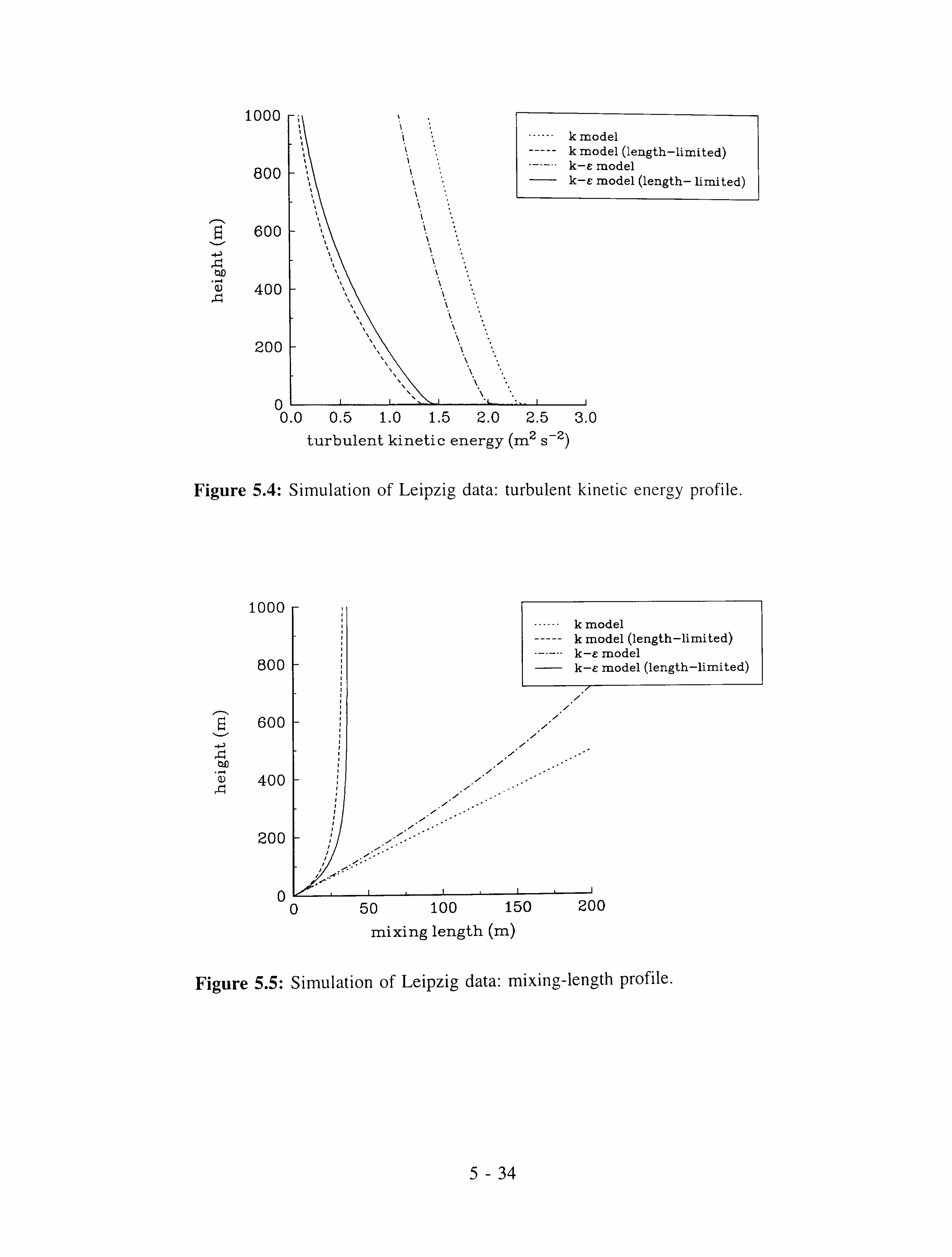
1000

800

600 ý

ý 400

200

I

F- 1

k model k model (length-limited) k-e model k-e model (length- limited)

k model k model (length-limited) k-E model k-e model (length-limited)

011 .I 0.0 0.5 1.0 1.5 2.0 2.5 3.0

turbulent kinetic energy (m2 s-2)

Figure 5.4: Simulation of Leipzig data: turbulent kinetic energy profile.

1000

800

600

400

200

11 11, .1..

i i

50 100 150 200

mixing length (m)

Figure 5.5: Simulation of Leipzig data: mixing-length profile.

1400

1200

1000

I--, 800 .. ý

a0 600

400

200

k-E model (standard) k-E model (length-limited)

I

I riii

2468 10

windspeed (m s-1)

Figure 5.6: Stable boundary-layer simulation: mean wind speed profile.

----- k-c model (standard) k-e model (length-limited)

-10 0 10 20 30

angle from geostrophic (deg) 40

Figure 5.7: Stable boundary-layer simulation: turning of wind with height.

400

---- k-e model (standard) k-e model (length-limited)

300

. ý. ý

ý 200 an ... aý

100

U

, ý . . ýý.

0.0 0.1 0.2 0.3 0.4 0.5

turbulent kinetic energy (m2 s-2)

Figure 5.8: Stable boundary-layer simulation: turbulent kinetic energy profile.

400

---- k-e model (standard) k-e model (length-limited)

300

. -. ý ý

200

Q) ý

100

ý I 1

10 20 30

mixing length (m)

Figure 5.9: Stable boundary-layer simulation: mixing-length profile.

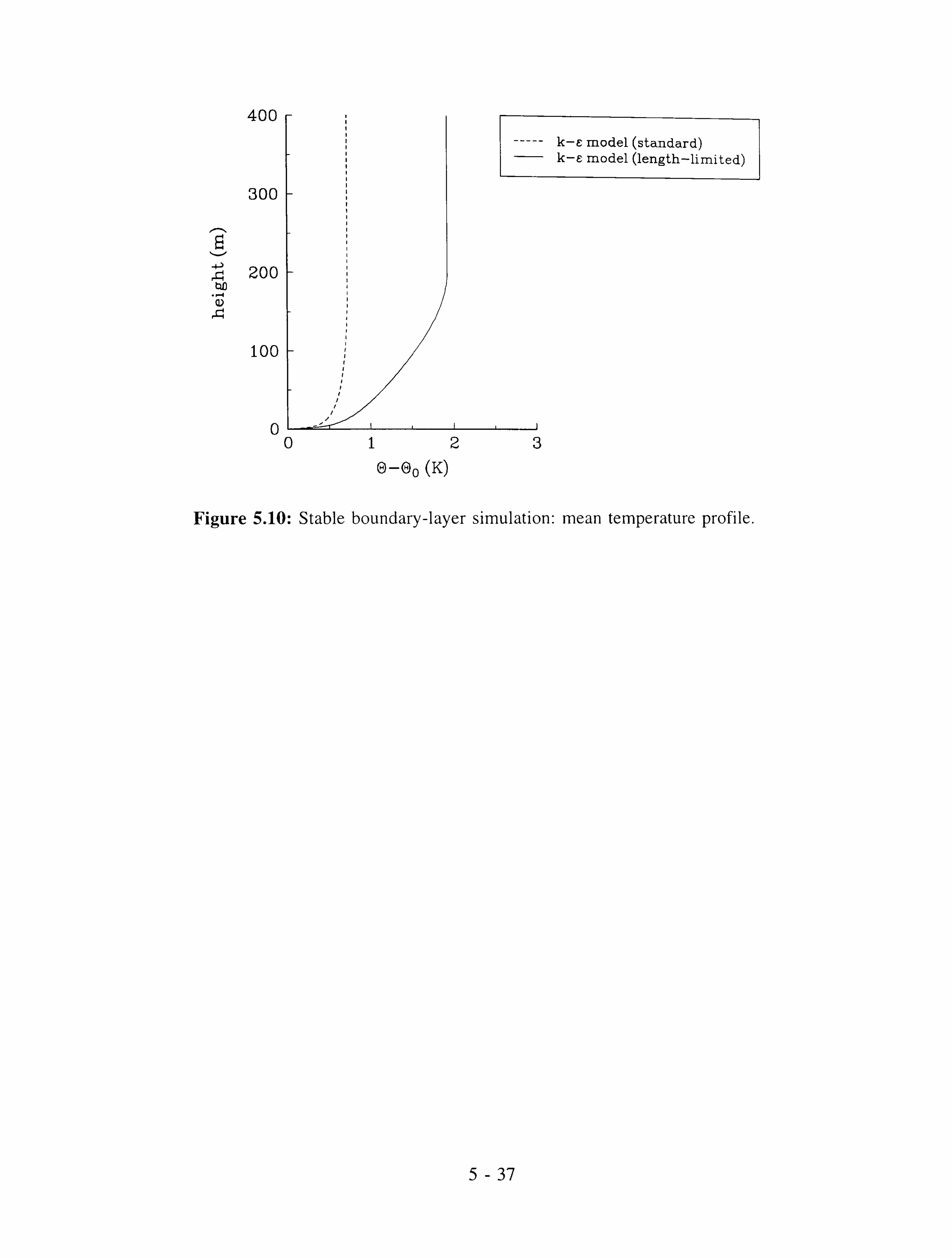
400

300

. -. ý

... ý 200 an ... ý ý

100

k-e model (standard) k-e model (length-limited)

ý ý , ;ý

0 1

0123

0-e0 (K)

Figure 5.10: Stable boundary-layer simulation: mean temperature profile.

1000

800

600

..., 400

200

1maz=(ý/ß)L 1maz-(ý/ß)A 1ý=0.68v,

r/N 1ý=v�/(dU/dz)

i ýi i

Iý ý

!iI

i ý ý

0 _j.

02468

Windspeed (m s-1)

10

Figure 5.11: Stable boundary-layer simulation: different limits on vertical mixing.

1000

800

600

ý

... 400

200 0

ý-kT II1III

468 10 12 14 16

windspeed (m s-1)

0

length-limited k-E model " Cardington data

Figure 5.12: Simulation of Cardington data: mean wind speed profile.

length-limited k-E model " Cardington data

-10 0 10 20 30 40

angle from geostrophic (deg)

Figure 5.13: Simulation of Cardington data: turning of wind with height.

500

400

300

. r.. i

200

100

O L. -I IIIIII

0.0 0.1 0.2 0.3 Flux Richardson number, Rf

Figure 5.14: Simulation of Cardington data: flux Richardson number profile.

CHAPTER 6.

Comparison With Experiment

Computational fluid dynamics is now used extensively both for investigating generic effects

in simple flows and as a predictive tool for real geometries. The admissibility of results in

either application should be treated with a healthy scepticism unless there is supporting

evidence from comparison between predictions and reliable experimental data. With this in

mind, the performance and limitations of the SWIFT code have been investigated by

comparing its predictions with two experimental data sets for dispersion in complex terrain:

the "Russian Hill" (RUSHIL) wind-tunnel study of Khurshudyan et al. (1981) and the United

States Environmental Protection Agency's field experiment at Cinder Cone Butte (Lavery et

al., 1982).

In the RUSHIL wind-tunnel study mean-velocity, turbulence and concentration profiles were

measured in neutrally stratified flow over symmetric two-dimensional hills, varying the hill

length-to-height ratio and the source location. The two-dimensional mean-velocity field with

well-defined approach-flow profiles formed a good test case for the turbulence model

modifications described in Chapter 4 to accommodate streamline curvature and streamwise

pressure gradients within an eddy-viscosity framework. The steepest topography promoted

flow separation which, in some cases, enveloped the emitting stack. This is not easily

accounted for in typical gaussian diffusion models.

The Cinder Cone Butte field trials involved the release of a tracer gas in highly stable flow

upwind of an approximately axisymmetric isolated hill. Field experiments were complemented

by laboratory simulations in a salinity-stratified towing tank. By contrast with controlled

conditions in a laboratory, inflow profiles were far less well-defined in the full-scale

experiment and the application to real terrain required the writing of surface-fitting routines

to interpolate for the local height of topography at horizontal grid nodes.

6.1 The Russian Hill (RUSHIL) Wind-Tunnel Study

The RUSHIL study (Khurshudyan et al., 1981) was part of a joint Soviet-American program to develop models for flow and dispersion of pollutants in hilly terrain. Wind-tunnel

simulations were conducted in the Fluid Modelling Facility of the US Environmental

Protection Agency (EPA) in North Carolina and the results compared with theoretical models developed by Soviet investigators. These models - described in an Appendix to the EPA

Report - were of comparatively simple type. The first, QPM (Quasi-Potential flow Model),

assumed the streamlines to be those predicted by potential-flow theory and, by conformal

transformation, reduced the problem to one of diffusion over a flat surface, which could then

be used to give surface concentrations for specified velocity and eddy-diffusivity profiles. The

second, WMDM (Wind-Measurement-using Diffusion Model). generated a mass-consistent

velocity field from actual point measurements of velocity, calculated an eddy diffusivity on

the basis of turbulence measurements and theoretical assumptions and then solved the

advection-diffusion equation numerically. The primary failing of the potential flow model was

its inability to account for the asymmetry of the flow, which led to unsatisfactory results when

a concentration maximum was recorded on, or downstream of, the lee slope, whether or not

the flow separated. On the other hand, reconstructing the velocity and turbulence field from

experimental data required a fairly high density of measurement points. It was hoped that a

full numerical solution would be able to overcome the deficiencies of both these models.

Descriptions of the experiment are to be found in the original Laboratory Report

(Khurshudyan et al., 1981), but data used for comparison here comes from the analysis of

Trombetti et al. (1991) where, in particular, the flow data has been smoothed to overcome

inherent scatter and the deficiencies of hot-wire measurements in recirculating flows.

6.1.1 Summary of the Wind-Tunnel Study

In the EPA wind tunnel a deep rough-wall boundary layer was developed using a combination

of an inlet fence and distributed surface roughness (10mm gravel). Sufficiently far downwind

of the fence the flow was adjudged to be slowly developing, mean-velocity and turbulence

6-2

profiles approximating those of a neutrally stratified atmospheric boundary layer with depth h of order 1 m, roughness length z0=0.157mm and friction coefficient u. /U-=0.047.

Flow measurements were made around two-dimensional symmetric hills of varying steepness. The majority of measurements were made with the same hill height, H=117mm, and with a free-stream wind speed U-=4m s' , giving a Reynolds number Re=U.

_H/v=3.1x10`. The hills

were designated H3, H5 and H8 according to their length/height ratio a/H and their shape was given parametrically by

1 x= =ýý1 +" 2 ý2+m2((I2-ý2)

2

z= ým

a2ý2 1-a ý2+rn2(a2-ý2)

ý2 U

iý <q (6.1)

where m=n+Jn2+1 and n=H/a is the average slope. (This particular shape was chosen to

allow conformal transformation in the potential flow model. ) In the wind-tunnel study flow

separation was observed on the lee slope of hill H3 but not H8. This was confirmed by the

computations undertaken here.

Diffusion experiments were carried out with an ethylene tracer emitted from a 15mm-diameter

porous sphere, providing an approximately neutrally buoyant, isokinetic release, independent

of the local wind direction. Source locations were at the upwind base (U), summit (S) and

downwind base (D), with various release heights.

6.1.2 Summary of the Flow Calculation

Numerical computations were undertaken over flat terrain and over the three hills using the

k-c turbulence model and its curvature-dependent and streamwise-pressure-gradient

modifications described in Chapter 4. Flow calculations were carried out on a two-

dimensional grid using the terrain-following curvilinear coordinate transformation defined in

Chapter 3. The computational domain extended a distance ±40H up and downwind of the hill

summit and to a vertical height 13.7H, the latter corresponding to the height at which the

6-3

free-stream velocity was measured in the wind tunnel (1.6m). Limited grid-dependence tests (to be described later) were undertaken with various different grids (a coarse mesh i; illustrated in Figure 6.1) but the majority of calculations used a non-uniform grid with 100 nodes symmetrically disposed about the centre of the hill in the streamwise (x) and 80 nodes in the vertical (z) direction. The minimum control-volume dimensions were 0.1HxO. 004H at the summit of the hill. The grid spacing was allowed to expand uniformly upwind, downwind

and in the vertical according to a geometric progression, the common ratio being 1.07 in all three directions.

Transport variables were specified at inflow by:

u* ln(z/zo) U=K

U ý

W=0

k

E=

Cµ 1/2u? (1 _z/h)2 1k

CO C 3/4k 3/2

µ

KZ

zsh

z>h

(6.2) z<0.9h

z>0.9h

corresponding to a zero-pressure-gradient equilibrium boundary layer of depth h, with a

quadratic fall-off in turbulence energy with height. For the given value of u*/U_=0.047, h and

k- were such as to make the mean-velocity and turbulent kinetic energy profiles continuous.

Zero longitudinal gradient (a/ax=0) was assumed for all variables at the downstream

boundary. Wall functions were invoked to apply the boundary conditions appropriate to a

rough wall on z=zs(x). The upper boundary condition requires some explanation. In the wind-

tunnel study the roof was raised locally over the hill to overcome blockage effects and

maintain a constant free-stream velocity - this zero-pressure-gradient condition being deemed

the appropriate way of simulating unbounded atmospheric flow. In the numerical simulation

the longitudinal velocity was maintained at a constant value on the upper boundary (U=U-)

whilst a small net mass flux was allowed through the boundary by updating the normal

velocity W on each iteration to satisfy continuity: aW aU

+aV Neumann boundary az ax ay

6-4

conditions (zero normal gradient) were used for k and £ on the upper boundary.

There is an important point to be made here about pressure boundary conditions. With the

staggered velocity arrangement on a cartesian mesh, pressure boundary conditions are

redundant since a velocity component (whose value is determined by some independent

boundary condition) is stored on the domain boundary, whilst the pressure gradients which drive the internal velocity field depend only upon internal pressure nodes. Thus, for a

staggered cartesian grid, values of pressure at the boundary nodes are irrelevant as far as the

flow dynamics is concerned: their values do not enter the discretised equations. The same is

not true in curvilinear coordinates because, in that case, the pressure gradient along a cell face

may enter the explicit source term. This occurs in the present application on the surface of

the hill. An appropriate pressure boundary condition to use is a`P/an2=0; that is, linear

extrapolation.

The governing equations were discretised and solved with the procedures documented in

Chapter 3, using the Van Leer harmonic scheme for advection and the SIMPLEX algorithm

to handle pressure-velocity coupling. The algebraic equations were solved by line-by-line

iteration in conjunction with the tri-diagonal matrix algorithm and the solution of the pressure-

correction equation accelerated using the anticipated-correction method.

6.1.3 Flow Comparison

The model hills in the RUSHIL study were of "moderate" slope; that is, sufficient to exhibit

marked flow asymmetry and, in the case of hill H3 at least, to cause flow separation on the

lee slope. This was confirmed in the numerical simulation (Figure 6.2).

Comparison of k-c Turbulence Model Variants

In passing over a hill an air parcel experiences considerable cross-stream and alongwind

acceleration. As we have already noted in Chapter 4 these departures from simple shear due

6-5

to curvature and streamwise pressure gradients respectively can have profound affects on the turbulent stresses which are not accounted for within linear, isotropic eddy-viscosity models such as k-E. Where only the cross-stream diffusion of momentum is significant, however. it is possible to frame modifications to the standard k-E model to accommodate these additional strains, at least insofar as they affect the mean-velocity field.

In the RUSHIL experiment the deep boundary-layer flow over hill H3 was observed to separate on the lee slope and this therefore forms a suitable test case for predictions of boundary-layer separation over a curved surface. Computations were performed with three of the k-c variants described in Chapter 4:

" standard k-c model; constants as in Chapter 4;

" k-c model with modification for curvature effects:

Cý IL

Cµ0

1 +442t2öU U

an k

(6.3)

k-E model with modification for streamwise pressure gradient:

PE = CE1 ~ [CE1II CElvt(ZJ)2] 1

(6.4) ýE ýE

In each case the turbulence timescale is iE=k/E.

Figure 6.3 shows vertical profiles of the x-velocity component at the upwind base, summit

and downwind base of the hill. At the upwind base all computed profiles are almost

coincident with the experimental data. Over the summit the computations indicate nearly

uniform velocity over several hill heights (as in the experimental measurements) and

maximum speed-up factors DU/Ua (Figure 6.4) in excess of 1.0. The discrepancy at lower

heights (z<O. 1H) which is revealed by the logarithmic vertical scale may arise from the nature

of the distributed roughness elements used in the wind tunnel and the definition of the zero-

plane displacement - experimental heights are measured from the top of the gravel which, at

nominal diameter 10mm, was a not inconsiderable fraction of the hill height. However, the

difference may also be a consequence of the implied structure function Cµ (ti/k)Z, which is

6-6

generally accepted to be lower over rough surfaces. The greatest distinction between k-c

variants is apparent at the downstream base of the hill. Here, although the standard k-c model does admit separation and reversed flow, the dissipation modification (in response to

streamwise strains) does a much better job of predicting the upslope velocity, the depth of the

recirculating-flow region and the sharp velocity gradients in the shear layer extending from

the separation point. The difference may be attributed to the excessive levels of turbulence

generated by the standard model in flows subject to streamwise strains, which tend to smear

out the large velocity gradient across the shear layer. This overly diffusive phenomenon has

been well-documented in other flows. Reduced turbulent transport in the modified model also

meant that the distance to reattachment (5. OH downstream of the summit) was greater than

with the standard model (4.1H), although still short of the experimentally observed 6.5H.

Perhaps surprisingly, the curvature modification had little overall impact on the mean-velocity

profile, particularly given the acknowledged sensitivity to streamline curvature exhibited by

turbulent flow in ducts. A partial explanation has already been noted in Chapter 4: the

curvature-dependent factor only departed significantly from unity at heights where the mean-

velocity perturbation was essentially inviscid. At lower heights the dissipation timescale, k/E,

was considerablylsmaller than the harmonic mean of those associated with curvature and

shear ( aU

SUS), which we have identified as the appropriate measure of the effect of an Rc

curvatu e. We can make an estimate of the size of the curvature-dependent factor for

boundary-layer flow over low hills. For a boundary layer in approximate equilibrium we have

2 k -1/2 KZ 3U5 US UT ln(z/zo) (6.5)

ýE EN

Cµ

UT ' an Rc

x2Z Rc

so that the curvature-dependent term is approximately

2 aUs Us ln(z/z0) z 'Ean Rc - Cµ Rc

(6.6)

The inner-layer height Q (Chapter 2), being a measure of the height over which turbulent

shear stresses play a significant role in the mean momentum balance, is given by

Q ln(Q/zo) - 2x2L (6.7)

where L is the horizontal length scale, and hence the condition that curvature effects on turbulence reflect back on the mean flow is

2x2 L Cµ R,

(6.8)

For any given shape of hill, Rc. min°`L

2/H, so that (6.8) becomes a condition on the slope parameter HIL.

That curvature may still have a significant impact upon the turbulence energy is illustrated

by computed profiles of turbulent kinetic energy over the summit of the hill (Figure 6.5). In

this instance the production of k is apparently enhanced by the unstable (concave) curvature

on the upwind slope of the hill. The curvature modification does bring about some improvement in the predicted turbulence levels, although still well short of the experimental

values. (In the data made available for the comparison only rms fluctuations 6u and 6,,, were

available and k=1/2((7ü+62+62. ) had to be derived on the assumption that 61-1/2(ßu+ß)

The bottom line is that ... for the mean flow in a deep turbulent boundary layer the response

of the turbulent length scale to streamwise pressure gradients is far more significant than the

effects of streamline curvature. (The same is not true for thin boundary layers in curved ducts

where streamline curvature effects on the normal stresses may give rise to complex secondary

flows. ) Accordingly, a single k-£ variant - the preferential response of dissipation to

streamwise strains - has been used for all remaining calculations in the RUSHIL comparison.

Effect of Hill Aspect Ratio

Wind-tunnel measurements were made with hills of length-to-height ratio a/H equal to 3,5

and 8. Steady flow separation was recorded for hill H3 but not H8. In the intermediate case.

H5, the laboratory report noted (intermittent) separation, although the time-averaged velocity

profile does not show this in either the analysed flow data or the numerical simulation.

6-8

Figures 6.6-6.8 show mean-velocity profiles (x-component) computed at the upwind base. summit and downwind base of each hill. In each case agreement with experiment is excellent, particularly in respect to the maximum speed-up at the summit. This confirms the effectiveness of comparatively simple turbulence models in predicting the dominant shear stress - and hence the mean flow - in perturbed deep boundary layers. If agreement was equally good in other respects then turbulence modellers would be out of a job. However, the inadequacy in predicting turbulent kinetic energy (Figure 6.5) seems likely to assure them of gainful employment for some time to come. Although the experimental profiles are subject to the previously mentioned proviso that the crosswind normal stress 6,, had to be estimated in order to evaluate k, there is still considerable discrepancy between predicted and measured

values. This deficiency is likely to affect concentration calculations significantly since it is

the turbulent stresses which are primarily responsible for plume dilution.

Grid Dependence Tests

A number of computations were undertaken to assess the grid independence of results for the

steepest hill H3. Meshes both coarser (A) and finer (C) than the primary grid (B) were

considered and their parameters are given in Table (6.1).

Grid Number of nodes Minimum control-volume dimensions

A 60 40 0.1 0.004

B 100 80 0.1 0.004

C 200 160 0.05 0.002

Table 6.1: Grids used in the flow calculations for hill H3

In each case the x-grid lines were symmetrically disposed about the hill centre with minimum

separation at x=0 and uniform expansion upwind and downwind. The minimum separation in

6-9

the vertical was at the lower boundary and the grid was allowed to expand uniformly to the top of the domain. The overall dimensions of the computational region (-40<_r/H<_40. 0_<z/H<_13.7) were the same in all cases.

Profiles of longitudinal mean velocity and turbulent kinetic energy for the three grids are shown in Figures 6.9 and 6.10 respectively. The profiles are almost coincident, as. in fact, are the separation and reattachment points. This gives satisfactory assurance of both grid independence and the smallness of the truncation error in the Van Leer advection scheme.

6.1.4 Concentration Comparison

The previous Section described the numerical simulation of turbulent flow over two-

dimensional hills of moderate slope. We turn our attention now to the simulation of dispersion

from a point source within the perturbed flow.

The release was assumed passive: that is, it had no impact on the flow and so could be

computed independently of the flow calculation. In this exercise the mean velocity and eddy

viscosity were interpolated onto a second grid, selectively refined near the source and

extending only a short distance upwind. An example is shown in Figure 6.11. Since the

concentration distribution was fully three-dimensional the two-dimensional flow field was also

parallel-mapped in the lateral (v) direction.

Although a point-source release was simulated using the practice described in Chapter 3,

whereby concentrations were analytically specified in the vicinity of the nominal emission

point, the actual source in the wind tunnel (a 15mm-diameter permeable sphere) was

comparatively large compared with the hill height (117mm). Thus the additional complexity

of an imbedded analytical domain was probably redundant in this instance.

It quickly became apparent that concentrations predicted by an isotropic eddy diffusivity v/6-

were consistently higher than measured concentrations. A typical vertical profile through the

plume for a release height h,. =H in flat terrain is shown in Figure 6.12. Concentrations are

6-10

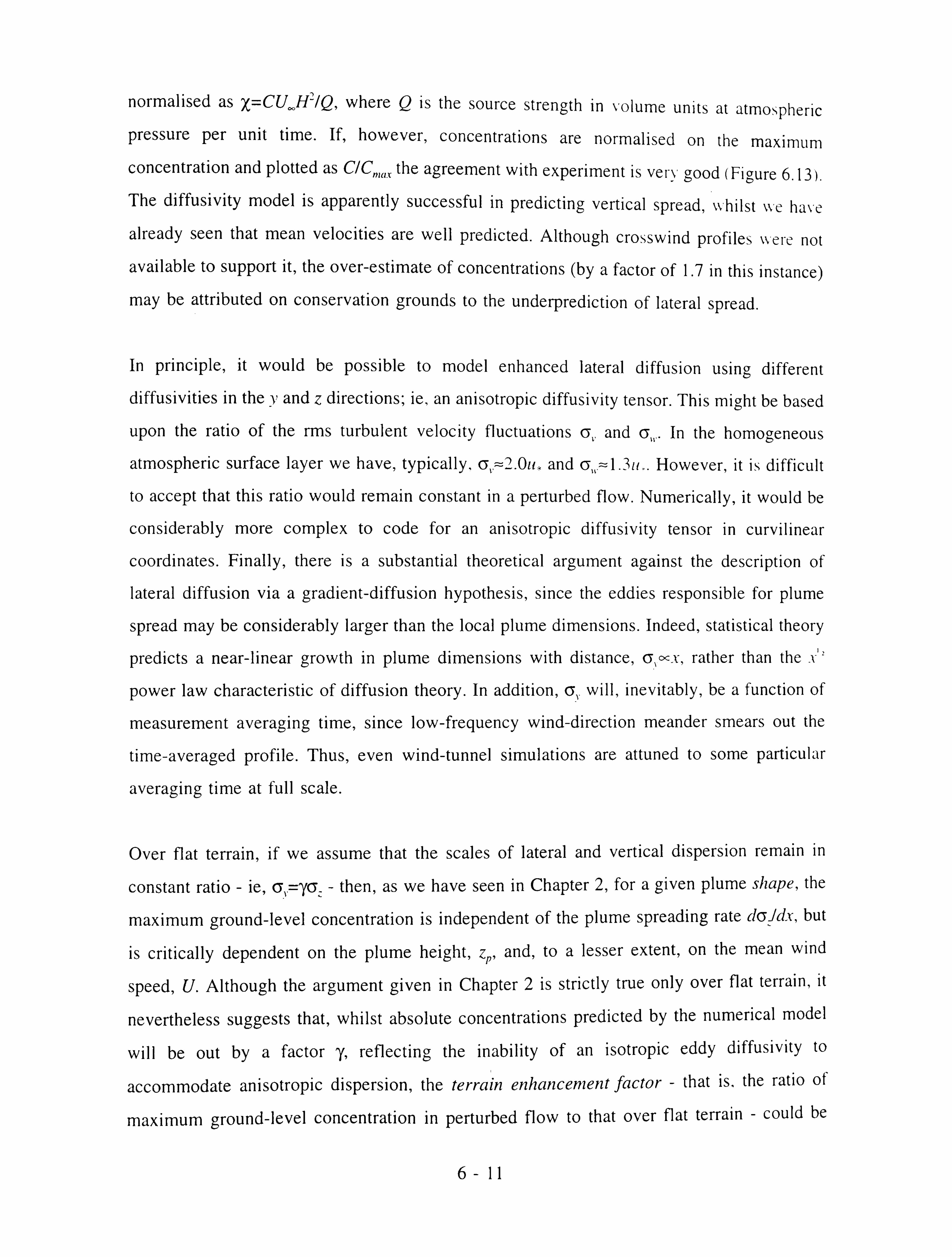
normalised as x=CU_H2/Q, where Q is the source strength in volume units at atmospheric pressure per unit time. If, however, concentrations are normalised on the maximum concentration and plotted as C/C,,.,

C the agreement with experiment is very good (Figure 6.13). The diffusivity model is apparently successful in predicting vertical spread, whilst we have

already seen that mean velocities are well predicted. Although crosswind profiles were not available to support it, the over-estimate of concentrations (by a factor of 1.7 in this instance)

may be attributed on conservation grounds to the underprediction of lateral spread.

In principle, it would be possible to model enhanced lateral diffusion using different

diffusivities in the y and z directions; ie, an anisotropic diffusivity tensor. This might be based

upon the ratio of the rms turbulent velocity fluctuations 6,, and ß,.. In the homogeneous

atmospheric surface layer we have, typically, ß,, =2. Ou and However, it is difficult

to accept that this ratio would remain constant in a perturbed flow. Numerically, it would be

considerably more complex to code for an anisotropic diffusivity tensor in curvilinear

coordinates. Finally, there is a substantial theoretical argument against the description of

lateral diffusion via a gradient-diffusion hypothesis, since the eddies responsible for plume

spread may be considerably larger than the local plume dimensions. Indeed, statistical theory

predicts a near-linear growth in plume dimensions with distance, 6, ocx, rather than the x':

power law characteristic of diffusion theory. In addition, ß,. will, inevitably, be a function of

measurement averaging time, since low-frequency wind-direction meander smears out the

time-averaged profile. Thus, even wind-tunnel simulations are attuned to some particular

averaging time at full scale.

Over flat terrain, if we assume that the scales of lateral and vertical dispersion remain in

constant ratio - ie, 6, ='y6` - then, as we have seen in Chapter 2, for a given plume shape, the

maximum ground-level concentration is independent of the plume spreading rate doJdr, but

is critically dependent on the plume height, zn, and, to a lesser extent, on the mean wind

speed, U. Although the argument given in Chapter 2 is strictly true only over flat terrain, it

nevertheless suggests that, whilst absolute concentrations predicted by the numerical model

will be out by a factor 'y, reflecting the inability of an isotropic eddy diffusivity to

accommodate anisotropic dispersion, the terrain enhancement factor - that is, the ratio of

maximum ground-level concentration in perturbed flow to that over flat terrain - could be

6-11

simulated accurately, provided the mean-flow calculation is correct. Moreover, 'since ß_ 1S

apparently predicted well, so too should be the location of the concentration maximum.

This expectation is largely confirmed by the results of the simulation. We consider first of

all a series of releases from source locations around hill H3. As has been demonstrated, the

numerical model correctly predicts flow separation from the lee slope. Figure 6.14 shows

predicted concentration contours on the vertical symmetry plane for a succession of releases

at different heights above the downwind base of the hill. For the lower release heights (H/4

and H/2) material is released within the recirculating-flow region and is spread in all directions from the source. The release from height H lies outside the separated flow, but

outlying parts of the plume still diffuse across the separation streamline and are then swept back upstream. Figures 6.15 and 6.16 plot ground-level concentrations on the plume centre-

line as a function of distance downwind of the source for various release heights. In the first

case, concentrations are normalised in the standard fashion as x=CU, H2/Q. As anticipated,

the numerical predictions are too high due to an underestimate of crosswind spread. In the

second case concentrations have been non-dimensionalised by the concentration maximum

(computed or measured as appropriate) over flat terrain, producing very good agreement in

terms of the maximum concentration and its location. Underprediction of lateral spread,

however, leads to a smaller rate of decay of concentrations with downwind distance than is

observed in the measurements.

Note that the effect of the recirculating-flow region (or "cavity") is evident in both

computations and measurements, with significant ground-level concentrations being recorded

upstream of the source. The region of high concentrations is very well predicted, consistent

with an accurate computation of the dimensions of the recirculating-flow region.

Two additional features associated with sources in the recirculating-flow region are apparent

in both computations and measurements and deserve special emphasis because they form the

basis of modifications to semi-empirical atmospheric dispersion models to account for regions

of recirculating flow associated with, for example, large buildings (Robins, 1983; Apsley.

1988). The first is that ground-level concentrations are fairly uniform over much of the region

of reversed flow: that is, the long residence times in the cavity (in two dimensions material

6-12

can only cross the separation streamline by diffusion) and enhanced levels of turbulence ensure that the recirculating-flow region is well-mixed. The second feature is the sharp fall-off in concentrations downwind of reattachment, with concentration distributions almost the same for all sources within the recirculating flow (hs=H/4 and h,. =H12 in this instance). In a simple model of plume dispersion, when the source lies inside or near a region of separated flow,

that region is assumed to be well-mixed and to form an extended area source for receptors downstream. Concentrations within the cavity may be estimated as

CR = QRTR

(6.9) VR

where V. is the volume and TR a typical residence time, based upon cavity dimensions and the approach-flow wind speed (see, eg, Fackrell, 1984). For sources internal to the cavity QR

is the actual release rate. For external sources the cavity forms a secondary source with QR

estimated by the rate of diffusion across the boundary surface, or by inverting (6.9), with CR

the average concentration on this surface.

There are also a number of qualitative similarities between these predictions and the

measurements of Castro and Snyder (1982), who performed wind-tunnel simulations of dispersion from sources downwind of (sharp-edged) hills, including a two-dimensional ridge

(hill CX in their paper). For their case of a source height h, =H/4 at . k, _/XR=0.5 (roughly

equivalent to the downwind base of the hill in our study) they observed that the ground-level

concentration maximum occurred between the source location and the hill crest, due to the

reversed flow between these two. Lateral ground-level concentration profiles between hill

crest and source station had "shapes characteristic of very narrow plumes (arising from

immediate advective and diffusive effects) superimposed on much wider and weaker

background plumes that arise, no doubt, from the recirculation, with subsequent spreading

and diluting of this initial narrow plume" - their Figure 22. A lateral profile taken at the

downstream end of the recirculating flow showed no such double structure. Both aspects - the

location of the maximum ground-level concentration and the superposed-plume structure - are

apparent in our own computations (Figure 6.17).

The final graphs for this test case (Figures 6.18-6.20) compare predictions of ground-level

6-13

centre-line concentrations from releases at height H14 above the upwind base, summit and downwind base of each of the RUSHIL models. In each case concentrations have been non- dimensionalised by maximum ground-level concentrations predicted or measured over flat

terrain. With the possible exception of the downwind source for hill H5, the results largely

bear out the interpretation of the earlier results: namely, that the computations are capable of

predicting terrain-enhancement factors and the location of the maximum ground-level

concentration, with particular improvements over simple models for steep topography

exhibiting flow separation. Hill H5 presents an awkward case for gradient-transport models

with time-averaged equations because, although there is no flow reversal in the mean, intermittent separation means that some material may be advected back toward the hill. The

concentration computations, which rely only on the time-averaged velocity, failed to

reproduce the long-term concentration levels between of the source and hill crest.

The general problem of predicting anisotropic dispersion and, in particular, crosswind spread

is likely to prove more of a problem for three-dimensional topography where crosswind

diffusion is coupled with lateral velocity shear.

6.2 The Cinder Cone Butte Field Dispersion Experiment

Cinder Cone Butte is an isolated, roughly axisymmetric hill about 100m high and 500m wide

in the state of Idaho, USA. In 1980 it was the site of a series of tracer-release studies,

yielding an extensive database for the validation and development of regulatory models for

pollutant dispersion in stably stratified flow near complex terrain.

The Cinder Cone Butte field experiment was a major element of the Complex Terrain Model

Development program funded by the United States Environmental Protection Agency (EPA).

The four main components of this program were:

" field observations and measurements;

" laboratory fluid modelling;

" data archiving and analysis;

" model development and evaluation.

6-14

For background, it is worth giving a brief summary of each component before concentrating on the field data chosen for the simulation.

Field experiments were conducted at Cinder Cone Butte (in 1980) and later at Hogback Ridge (in 1982). These were chosen respectively as approximately axisymmetric and mo- dimensional isolated hills. Tracer gases (SF6 and CF3Br) were used to establish the ground- level concentration distribution from elevated releases in stably stratified atmospheric

conditions. Concentration data was supplemented by meteorological measurements (wind

speed and temperature) at fixed sites and LIDAR and photographic observations of plume behaviour.

Laboratory fluid modelling was undertaken in a salinity-stratified towing tank at the EPA's

Fluid Modelling Facility in North Carolina. Coloured dye was injected upstream of scale

models of Cinder Cone Butte. Streamline flow patterns and the horizontal and vertical

dispersion of plumes were recorded by cameras above and below, and fixed with respect to,

model hills. Quantitative concentration measurements were made by extracting samples of the

dyed fluid through ports on a model surface for colorimetric analysis. In the Cinder Cone

Butte study fluid modelling was used in a number of ways:

before the field trials: -

to establish the location for a meteorological mast to characterise the undisturbed

approach flow;

" to predetermine suitable gas-sampler and camera locations for the field measurements;

after the field trials: -

to simulate at model scale plume dispersion behaviour in selected case-study hours.

Experimental data from the field experiments were extensively audited by independent

agencies, generating a substantial quality-assured archive. Data for the numerical simulations

presented here has been taken entirely from the first two Milestone Reports (Lavery et al.,

1982; Strimaitis et al., 1983).

A number of existing analytical dispersion models - VALLEY, COMPLEX I. COMPLEX II,

PFM (potential flow model) - were tested by the EPA against the experimental data. In the

6-15

light of the results two new models - "lift" and "wrap" - were developed. Their de, i`gnation

refers to the assumed behaviour of the plume centre-line. As we have seen in Chapter 2. in

strongly stratified flow energy considerations suggest that the fluid below a critical diividing-

streamline height H, is compelled to travel in roughly horizontal planes whilst that above H,

can be modelled as flow over a "cut-off" hill with base at the dividing-streamline height.

Plume dispersion behaviour in the two regions is treated by "wrap" and "lift" models

respectively. Both are essentially gaussian-plume models, but with parameters modified to

account for the topography. They have since been assimilated into CTDM (Complex Terrain

Dispersion Model) and its convective boundary-layer extension CTDMPLUS. for which a definitive technical formulation has been given by Perry (1992).

Here, we report the results of a computational-fluid-dynamical simulation of one particular

case-study hour (Experiment 206,0500-0600 local time). This case has been chosen because

it is considered representative of very stable atmospheric conditions, it presents the interesting

case of a release at, or very near, the dividing-streamline height, and it was the subject of a

laboratory fluid modelling study (Snyder and Lawson, 1981 ; Snyder, 1990).

Flow and diffusion were computed with the limited-length-scale k-c turbulence model

described in Chapter 5. This k-E variant attempts to limit the computed turbulent length scale

by some (externally specified) maximum scale In this instance we used a form suitable

for stably stratified boundary layers:

'max =K max(LMO, AMO) (6.10)

where LMO and AMo are the surface and local Monin-Obukhov length scales respectively. The

correction is imposed through an addition to the dissipation production term which, as we

have already seen in Chapter 5, has some similarities to Rodi's (1987) model based on the

local flux Richardson number. In fact, the main effect of the modification was to overcome

the excessively diffusive nature of the standard k-E model, which otherwise eroded the

approach-flow temperature profile so severely that the flow encountering the hill was

effectively neutrally stratified.

6-16

Since the Rossby number, Ro=U/fL, based on the horizontal length scale L. was large (--100 in this instance) the dynamical effect of Coriolis forces could be neglected and rotational effects were therefore excluded from the simulation. (When significant, however. rotational effects in stratified flows typically extend of a distance of order the Rossbv deformatio, i radius, IR=NH/f, which may be significant in flows around large scale features such as mountain ranges. )

6.2.1 Setting Up the Simulation

Geometry

The topography of Cinder Cone Butte was digitised (by hand! ) from the height contours in

the first EPA Milestone Report and mapped onto a rectangular grid by a local weighting

method. The terrain was smoothed around the edges of the domain to a flat plane

corresponding to the 3080ft (944m) level. (The zero level in the EPA Reports was the 3100ft

level, being the lowest closed contour, but about 5m above the base of the hill. )

As can be seen from Figure 6.21, Cinder Cone Butte is double-peaked, with the higher

(southern) peak at 3426ft (105.5m above the zero plane). A coordinate origin was chosen in

the draw between the two peaks (same location as the EPA Reports) and a rotated x-v grid

laid out with the new x-axis in the direction of the mean wind.

In the hour selected for the simulation (Experiment 206,0500-0600 local time) the mean wind

at the source height was from a bearing of 127°. SF6 was released at a rate of 0.062 gs -`

from a height of 35m above local terrain at a source location almost directly upwind; (595.9m

at bearing 123.6° or (x,, y, )=(-595m, -35m) in the coordinate system aligned with the approach

flow).

For computing the flow field the computational mesh employed 70x53x40 nodes in the _ß-. 1", z

directions respectively. In the streamwise direction the upstream boundary was set at _r=-

5000m and the downstream boundary at x=8000m. Lateral boundaries were set at v =±2500m

6-17

and the upper boundary at z=2000m. 27 nodes were placed symmetrically at equal (40m) intervals over the hill in both horizontal dimensions. Beyond this, uniform grid expansion ýý as employed to upstream, downstream and lateral boundaries with constant expansion ratios 1.20. 1.13 and 1.19 respectively. In the vertical the nearest internal node was 1m from the surface (ie, the minimum control volume height was 2m) and the grid was allowed to expand uniformly to the upper boundary. The constant expansion ratio was 1.14. Figure 6.22 shows the computational mesh laid over the topography of Cinder Cone Butte.

Inflow Profiles

The numerical procedure requires that transport variables (velocity components U. potential

temperature O, turbulent kinetic energy k and dissipation rate e) be specified as a function of height at inflow.

A salutary message that arose from the specification of the inflow profiles was that various "standard" profiles used with impunity by dispersion modellers bear little or no resemblance

to wind, temperature or turbulence profiles recorded in any particular experiment. This is not

to say that such deterministic profiles should not be used for regulatory assessment - just that

they should come with an appropriate health warning! Seriously, however, schemes for

deriving boundary layer parameters (such as friction velocity it. and Monin-Obukhov length

LMO) are not robust and may actually be misleading. A case in point is the "profile method"

of Van Ulden and Holtslag (1985) which uses the mean flow profiles to determine it- and L, ti10. Given:

" wind velocity U, at one height z,;

" potential temperature difference A between two heights z, and

then surface-layer similarity theories predict for stable conditions:

Ul =K [1n(zl/zo) + ßz, ILMOI

2

De= 03-82 =2U. [ln(Z3lz2) + ß(Z3 -Z2)I LM0] ß K agLMo

ý5

(6.11)

6-18

Eliminating it. we deduce

Ul

= agLMOýý(z1/ý +ßz, /LMO12

Aa [ln(z)z2) +ß (Z3 -Z2)/LMOý (6.12)

which could be solved (numerically) to determine LMO and thence u.. The problem is that individual realisations of atmospheric behaviour may be poorly represented by such diagnostic

profiles. Indeed a naive solution of (6.12) can (and in this case does) actually produce roots for LMO of the wrong sign! The only truly unambiguous way to determine surface momentum

and heat fluxes is to measure them.

On the other hand, even discounting instrument deficiencies, real-time measurements of flow

variables are subject to statistical and temporal mean variations in the flow, are limited in

resolution and, as in this instance, are limited in extent: the fixed meteorological mast yielded

little information about what was happening above 150m. It is clear, therefore, that judicious

use of theory is necessary to smooth, interpolate and extrapolate from the recorded

measurement data.

Inspection of the temperature data averaged over the hour of the experiment indicated a

potential temperature gradient approaching a constant value d0/dz=2.98x 10 Km -' as

approached the highest measurement level (150m). This is consistent with Monin-Obukhov

(surface-layer) similarity theory (see Chapter 5) where the potential temperature gradient is

expressed as

d0 6* -8ýw ö u?

dz KZ (1+ ß zILMO) ,

6* u* KagLMo

(6.13)

e approaching a constant value

ß` as zILMO-4°°. In fact it has often been observed that the

KL0 temperature profile conforms to the surface layer similarity form to heights considerably in

excess of z=LMO and, accordingly, we have chosen the asymptotic value of the temperature

gradient as a suitable means of evaluating the Monin-Obukhov length. Integrating (6.13)

yields

©= Oo +d [z + Moý(z/zý]

z. a 1 (. 14)

Given (dO/dz)c, =2.98x10-2K m-1, a least squares fit determines the free parameters =33n,

2.16°C and Monin-Obukhov length LMý This limiting temperature gradient gives a corresponding buoyancy (or Brunt-Väisälä) frequency

N= agd0"2 = 0.033s -1 (6.1

In general, the mean-velocity profile is not so accommodating as to support surface-laver

similarity profiles to any great depth. In this case we have chosen instead to fit a power-law

velocity profile

U(z)=Uo150 1' (6.16)

to the recorded wind data at 10,80 and 150m. (Due to an instrument failure at 40m the wind

speed estimated at this height in the EPA Report is considered too unreliable). Parameter

values were Uo=9.14 ms -' and n=0.90. The wind speed at the source height was about

2m s -'. This functional form was extrapolated to give the wind speed right to the top of the

computational domain. Coriolis forces were disregarded and uni-directional flow assumed at

the inflow boundary. During the field experiment wind speed and direction at the lowest

measurement heights (2m and 10m) were observed to be decoupled from the upper-level

winds.

The possible influence of gravity waves in the upper layer led us to consider the sensitivity

to inflow conditions and, in particular, to the stability profile. The full-scale experiment was

carried out during a nocturnal surface inversion and one might expect the temperature profile

to approach neutrally stable (adiabatic) conditions further aloft. Accordingly, a few

calculations were also carried out with alternative fits to the potential temperature and wind

speed data having the exponential form

6-20

N= Noe -z/he or

U= Uo(1-e -, Ih,, )

2

O= Oo +° he

(1-e -2z/he) 2ag (6.17)

Least-squares fits to the same data produced free parameters 00=-1.50°C, N�=0.04-9ý-',

he=267m, whilst Uo=19.8m s -` and hu=251m.

The two sets of profiles are illustrated in Figure 6.23. They are almost coincident over the height range of the approach flow measurements and, therefore, do not affect the computation

of the dividing-streamline height. However, the nature of internal gravity wave motions in the

atmosphere can be significantly affected by the undisturbed-flow density profile, with uniform

stratification permitting long waves to propagate vertically unattenuated (in the absence of dissipation). Also, the impermeable upper boundary of the computational domain reflects

wave energy and undamped motions could exhibit resonance at the normal modes.

The turbulent transport variables - turbulent kinetic energy k and its dissipation rate s- were

determined at inflow by using SWIFT to solve the one-dimensional turbulence equations with

mean velocity and potential temperature fixed. This was deemed expedient since

experimentation with two-dimensional flow calculations over flat terrain indicated that the

turbulence variables evolved very rapidly to a form determined by the mean profiles.

Other Boundary Conditions

As described above, transport variable values were fixed at inflow (Dirichlet boundary

conditions). Homogeneous Neumann boundary conditions (zero normal gradient) were used

at the downwind boundary.

The lower boundary was taken to be a uniformly rough wall characterised by roughness

length z0=0. I m. The lower boundary conditions were determined by the standard wall-function

treatment, implemented through an effective wall eddy viscosity. The potential temperature

boundary condition was the most difficult to specify, temperature being the only flow variable

6-21

whose surface value is affected by factors external to the flow (radiation flux. soil heat flux. etc. ). Here, local equilibrium, aFelan=0, was assumed, where F. is the heat flux normal to the surface, which is determined essentially by the heat transporting capacity of the turbulent flow.

The upper computational boundary, z=D took the form of that mathematical artefact -a stress- free rigid lid - with zero normal velocity and zero normal gradient (a4/an=0) for other

variables. Similar boundary conditions were applied at the lateral limits of the domain,

and v=v,,,., 1.

6.2.2 Flow Features

One of the difficulties in visualising three-dimensional flows is that, unlike our eyes which

give us stereoscopic vision and some idea of distance, hard-copy output is necessarily a two-

dimensional projection. A confused picture may emerge if information from different planes

is superposed: streamlines appear to cross and the flow appears to lack mass consistency. This

is a particular problem for streamlines in three-dimensional separated flows.

For the flow simulated here the dividing-streamline height was calculated to be H, =32m;

(fractionally less than the source height). Idealised flow models envisage distinct regions -. <H,

where the flow travels in horizontal planes around the hill and z>H, where it travels over the

top in a form similar to neutral flow. It seemed appropriate to look for such a distinction in

this simulation.

What was actually found was that:

(i) at low levels there was indeed significant lateral divergence with the flow following

the contours of the hill

... but that ...

(ii) the region of horizontal flow/lateral divergence was of depth approximately 15m: ie,

considerably less than the calculated dividing-streamline height;

... and that ...

6-22

(iii) there was an intermediate region of similar depth where the flow changed Smoothly from being essentially horizontal to showing little lateral displacement.

These features are illustrated by the vector plots and streamline diagrams in Figures 6.24 - 6.28.

Vector plots formed by taking horizontal slices through the hill at heights of lOm and 35m

are shown in Figures 6.24 and 6.25. The arrow length has been scaled on the approach tlowv

velocity at each height so that we may note immediately the much greater relative variations in velocity at the lower height. The computed flow follows the contour of the hill at 10m (the

lowest terrain height marked) but at 35m is moving considerably across the topographic

contours.

If instead of taking a horizontal slice we interpolate for the velocity vectors at a displaced

height of 10m above the surface we obtain the vector plot shown in Figure 6.26. Attention

is drawn to three qualitative aspects of the flow: substantial velocity speed-tip over the

summit (greater than a factor of 3), a region of separated recirculating flow on the lee slope,

and considerable lateral asymmetry reflecting the actual shape of the Butte. These features

violate two commonly used simple approximations: the linearisation of the flow equations and

the idealisation of the hill as a single ellipsoid.

Streamline flow diagrams give a good indication of plume behaviour, particularly in the

highly stratified case where turbulent diffusion is small but the mean flow is substantially

displaced. Figure 6.27 shows integrated streamlines emanating from heights of 10,20 and

30m upwind of the hill. As anticipated from the vector plots there is a radical difference in

behaviour for the three initial heights with the lower streamlines being forced to circumvent

the hill while the more elevated streamlines pass over the top with comparatively little lateral

deviation.

Figure 6.28 shows streamlines integrated from the position of the source (. 1, =-595m,

v, =-35m in a coordinate system aligned with the approach flow). The streamlines are initially

separated by vertical intervals of 5m. Note that the streamline starting from a height of 20m

6-23

is advected into the separated flow region.

A number of observations are in order.

(i) Significant lateral divergence only occurs for streamlines starting below =1 5m; other streamlines pass over the hill.

(ii) Some streamlines are advected into the complicated recirculating flow in the lee of the hill. This bears out the observation that separated flow regions in three dimensions are not closed (or, indeed, easily defined) and, unlike their two-dimensional counterparts. material can enter by advection, even in steady flow.

(iii) There is a substantial downslope wind on the lee slope, which brings all the

streamlines computed here close to the surface downwind of the Butte. This is a

characteristic feature of stable flows where the internal gravity wave "attached" to the

topography may lead to maximum speed-up on the lee slope rather than the summit. Large near-surface lee-slope winds are also apparent in the 10m vector plot (Figure

6.26).

We shall go on to examine the effect that stably stratified flow has on the dispersion of

pollutants. One important effect which is seldom if ever incorporated into regulatory

dispersion models should be noted here. Enhanced lateral dispersion is often ascribed to the

effects of increased turbulence. In fact a far more important factor is the large horizontal

displacement of streamlines initially close together. Consider Figure 6.28 for example. An

initial vertical separation of just 15m leads to streamlines displaced horizontally by nearly

300m.

Some computations were undertaken to investigate the sensitivity of results to the inflow

profiles of wind speed and temperature. The flow patterns described hitherto have used a

power-law velocity profile and Monin-Obukhov similarity profile for temperature, the latter

tending to a constant buoyancy frequency for large As we have already seen in Section

6.2.1 an equally valid approximation to the upstream data can be achieved with a limited

depth of velocity/temperature shear and an effectively uniform-wind-speed, neutrally stable

layer aloft. The profiles are almost coincident over the height of the hill and, as confirmed

by the temperature isotherms in Figure 6.29, exhibit very similar flow behaviour despite the

6-24

radically different upper-layer stability profiles. The attached lee wave is. however, stronger

and of shorter wavelength for the "uniform-N" profile.

6.2.3 Concentration Calculations

An initial dispersion calculation was performed with the grid used to compute the flow

(called, not unreasonably, the "flow grid") and with the source distributed uniformly across

one control volume. The comparatively coarse grid meant that the large gradients of

concentration in the vicinity of the source could not be resolved and there was excessive

initial smearing, resulting in a wider plume and lower surface concentrations than might be

anticipated. However, taken together with the streamline diagrams this initial plot was used

as a guide to the positioning and refinement of a new mesh (the "concentration grid")

selectively refined near the source. Flow variables were interpolated onto this second grid,

also of 70x53x40 nodes, refined near the source and covering a smaller computational

domain: -200m<x-x, <2000m, -900m<v-vS<900m, O<z<300m. The smallest control volume

was centred on the source location with xyz dimensions 5mx5mx5m, and uniform expansion

was employed out to each domain boundary. The grid lines were symmetrically disposed

about v=vs, although preliminary calculations on the flow grid indicated the plume to be

deflected over the north-east (y<O) side of the Butte.

The resolution of flow and concentration grids is compared in Figure 6.30 and computed

ground-level concentrations in Figure 6.31. Concentrations are expressed in parts per trillion

(ppt) for easy comparison with the original data report. The gross behaviour of the plume on

the two grids is very similar, but closer inspection reveals a narrower plume and nearly 50%

greater maximum ground-level concentration in the latter case (1554 ppt as opposed to 862

ppt). The effect of using an imbedded analytic region to resolve plume behaviour near the

source was minimal in this instance, as the plume behaviour was dominated by the relative

deviation of streamlines in the strongly perturbed flow field.

In contrast with the dispersion behaviour over flat terrain (Figure 6.32) where the maximum

concentration in the plume remained elevated at several kilometres downwind, the plume in

6-25

the perturbed flow impacted directly on the upwind slopes of the Butte. As demonstrated by the streamline plots, material brought close to the ground is diverted laterally, resulting in a concentration distribution smeared across much of the north-east face (v<O) of the Butte. The impact of the plume on the terrain and the accompanying downslope spread are well depicted in the vertical cross-section through the plume on the upwind slope (Figure 6.33). Note the considerable crosswind shear over the depth of the plume as the lower regions are deflected

substantially more than elevated parts. This effect cannot be incorporated into standard gaussian plume models of dispersion with single length scales 6 and 6, characterising lateral

and vertical diffusion.

In contrast to uniform flow, the crosswind spread of the plume is largely due to the downwind

separation of streamlines initially close together. Although it is (turbulent) diffusion which

causes initial cross-streamline dispersion, plume spread is rapidly amplified by the subsequent divergence of streamlines. Moreover, in complex three-dimensional flow, stream tubes become

highly contorted and (in contrast to two-dimensional flows) there is no requirement for these

particular streamlines to come together again downstream.

A primary objective of this study was to compare the results of numerical simulation with

measured results, in this case ground-level concentrations obtained in the full-scale field

experiment. Figure 6.34 redraws the ground-level concentration contours predicted by SWIFT

with the recorded (hourly-averaged) data from the field study superposed. The maximum

recorded concentration is well-predicted by the numerical model. A pointwise comparison of

predicted and measured concentrations is not helpful, however, because it is clear from Figure

6.34 that the computations indicate material all being swept around the north side (y<0) of

the Butte whilst, in the full-scale experiment, significant concentrations were detected through

the draw between the peaks and on the southern slopes at times during the hour. This is a

salutary warning. In the computational model we have used a single hourly-averaged mean

wind direction. In reality, of course, the wind direction fluctuates, and, because the release

was very close to the centre-line of the hill, tiny changes of wind direction could lead to gross

changes in concentration fields as the plume switches from one side of the hill to the other.

The hourly-averaged concentrations obscure the fact that they were derived from intermittent

bursts of high concentration when the receptor lay under the path of the plume.

6-26

To examine this directional dependence additional calculations were undertaken with the

approach-flow mean wind direction backed through 5 and 10°. To minimise numerical errors arising from misalignment of grid lines with the wind vector, both flow and concentration

grids were rotated (and the topography re-interpolated) for each wind direction. Flow grids

were equally disposed with respect to the coordinate origin and concentration grids with

respect to the source for each wind direction. Results are shown in Figure 6.35. In all instances, the plume impacted on the surface, the higher concentrations for the wind bearing

of 117° being largely a consequence of the shorter geometric distance to the upwind slope for

this direction. As the approach-flow wind direction changed by a mere 10° the region of high

ground-level concentrations switched from one side of the Butte to the other, consistent with

the large spread of concentrations encountered over the hour during the field experiment.

In principle it would be possible to compute ground-level concentrations for each wind-

direction/wind-speed combination and provide a weighted concentration distribution given the

experimental speed/direction frequency matrix. This exercise was not undertaken because it

would demand considerable computational resources, and a breakdown of the experimental

data into speed and direction categories was not available. However, the relative distribution

of ground-level concentrations computed for each wind direction were in very good agreement

with those measured in the EPA towing tank (Snyder, 1990) where, of course, upstream

conditions were constant and well-defined. The towing tank simulations also confirmed the

great sensitivity to wind direction which led to hourly-averaged concentrations smaller and

spread more widely than those simulated in a laboratory or on a computer. In fact, the best

comparison between computations and field measurements in terms of plume location

occurred with a specified approach-flow wind direction of 122°. Experimental measurements

are superposed on ground-level concentrations computed for this wind direction in Figure

6.36. Whilst it may seem a little arbitrary to choose a wind direction different from that at

the source height it must be noted in defence that the wind direction shear recorded in the

field experiment was very large: the mean wind direction at 80m was steady from a direction

of 132°, whilst that at 10m fluctuated wildly, with an hourly mean value of 26°! According

to the qualitative judgement of the observers watching the plume approaching the hill, the

majority of this wind direction shear occurred below 30m.

6-27

A scatter plot of measured vs predicted ground-level concentrations is given in Figure 6.37.

It is clear that predicted concentrations are typically higher than those observed: in some cases

by a factor of 3 or more. The most likely cause is wind direction sensitivity. Small

fluctuations in the direction of the approach flow cause the plume to miss some of the

sampling points altogether at selected times during the measurement hour. The effect of

averaging over a long period is to "smear out" the measured distribution of ground-level

concentration.

I

N

Close-up of hill

ý Ni

12

10

8

6

4

2

0 -40 -30 -20

I

-10 0

x/H 10

I

I

20 30 40

Whole domain

Figure 6.1: RUSHIL experiment: mesh distribution for hill H3; (vertical scale exaggerated).

6-29

Figure 6.2: RUSHIL experiment: computed streamlines for hill H3.

H3 - summit

H3 - upwind base

10

I

ý

0.01 L

10

I

0.1

H3 - downwind base

! ý ý

s

0.1

001 1Y1ý'1.1

0.0 0.20.4 0.8 0.8 1.0 1.2 UAT.

0.0 02 0.4 0.8 0.8 1.0 1.2 UIIJo

Experiment k-E: standard k-E: curvature mod. k-e: dissipation mod.

U 0.01 0.2 0.0 0.2 0.4 0.8 0.8 1.0 1.2

UPo

Figure 6.3: RUSHIL experiment: longitudinal-velocity profiles for hill H3 using different k-s

variants.

SPEED-UP FACTOR Hill H3 - summit

10

0.1

0.01 0.0 0.2 0.4 0.6 0.8 1.0 1.2

AU/U0

Figure 6.4: RUSHIL experiment: relative speed-up factor (computed) over the summit of hill H3.

H3 - summit

Experiment k-s: standard k-c: curvature mod. k-c: dissipation mod.

\ N

0.01 '1,, "... III 0.00 0.01 0.02 0.03

k/Uö

Figure 6.5: RUSHIL experiment: turbulent kinetic energy profiles over the summit of hill H3

using different k-E variants.

H3 - summit

10

H3 - upwind base

10

9

8

7

8 10

6G

48

37

2e

0.0 0.2 0.4 0.8 0.8 1.0 1.2 U/U0

2

. _ý ., 0.0 0.2 0.4 0.6 0.8 1.0 1.2

0

Ultro

----- Experiment Computation

I 4

H3 - downwind base

-0.2 0.0 0.2 0.4 0.8 0.8 1.0 1.2

U/U0

Figure 6.6: RUSHIL experiment: comparison of velocity profiles over hill H3.

H5 - summit

10

9

H5 - upwind base B

7

10

9

B

7

8

4

Ultro

X; r

6

5

4

3

2

1

n ý 0.0 02 0.4 0.8 0.8 1.0 1.2

Ultro


10

9

8

7

B

4

H5 - downwind base

I

s[ 2 1r_,

_ n

A .1

1.0 1.2 0.0 0.2 0.4 0.6 0.8

U/vo


C

L

0.0 02 0.4 0.8 0.8 1.0 1.2

s Z- 1 n

6-33

H8 - summit

10

9

8

7

8

4

3

2

1

H8 - upwind base

r I d

0.0 02 0.4 0.8 0.8 1.0 1.2 U/Uo

10

9

8

7

6

4

3

2

1

o 0.0 0.2 0.4 0.8r 0.8 Uh/ýo

1.0 1.2


H8 - downwind base


H3 - summit

H3 - upwind base

10

I

s

0.1 G

10

I

ý

.00.2 0.4 0.8 0.8 1.0 1.2 U/U. 0.1

mesh A: 60 x 40 0.01' nni

H3 - downwind base

--- 0.0 0.2 0.4 0.8 0.8 1.0 1.2 ----- mesh B: 100 g 80 -'"=0.2 0.0 0.2 0.4 0.6 0.8 1.0 1.2 U/U. --- mesh C: 200 x 160 U/Uu

Figure 6.9: RUSHIL experiment: mesh dependence of mean-velocity profile for hill H3.

H3 - summit

101 mesh A: 60 x 40 mesh B: 100 x 80 mesh C: 200 x 160

10

\ N

10-

10- 0.00 0.01 0.02

k/-U2

0.03

Figure 6.10: RUSHIL experiment: mesh dependence of turbulent kinetic energy profile for hill H3.

_ ý

N

Figure 6.11: RUSHIL experiment: typical mesh for concentration calculations; (hill H3;

source location: downwind base; source height hs=H/2).

Vertical Concentration Profile Flat terrain; X/H=8

4

Computation " Experiment

\2 N

.ý

0 "

0 0

0 "

"

1

0

" "

0 0

"

0 " "

" " "

0

"

,"ý, ý, ý, ý, ý 0 0.0 0.2 0.4 0.6 0.8 1.0

CUH2/Q

Figure 6.12: RUSHIL experiment: dispersion over flat terrain - vertical profile through plume

at x-x, =8H. The source height is h, =H.

Normalised Concentration Profile Flat terrain; X/H=8

0.4 0.6 C/cmax

Computation Experiment

Figure 6.13: RUSHIL experiment: as previous Figure but concentrations normalised on C,,, (, 1..

. oo=- 2 200E+Ö0'

3 4.00E-00 4,8.00E-00 51 1.60E+01 6i3.20E+01

=3 N

2

1 -ý

0

7 8 9 10 11 12

6.40E+01 I 1.28E+02 2.56E+02 5.12E+02 1.02E+03 2.05E+03

x/H

(a) h, lH=0.25

(b) h, JH=0.5

x/H

(c) h,, lH=1.0

Figure 6.14: RUSHIL experiment: contours of x=CUH2IQ for three release heights over the

downwind base of hill H3. The separation streamline is also shown.

6-40

Ground-Level Concentration - Hill H3 Source at Downwind Base

1 00

Or 10 N

r :: D U

I

6

hS=H/4 - computed " hS=H/4 - experiment

hs=H/2 - computed " hS=H/2 - experiment -- hS=H - computed

m

downwind distance from source, (x-xs)/H

Figure 6.15: RUSHIL experiment: centre-line ground-level concentrations for hill H3: source location: downwind base.

Ground-Level Concentration - Hill H3 Source at Downwind Base

1 00

hS=H/4 - computed " hs=H/4 - experiment

X

ý 10 ö

U

U

01 0 ý ý c (L) U

ö 0.1 U

0.01 -5

£

A

hs=H/2 - computed hs=H/2 - experiment hs=H - computed

05 10 15 20 downwind distance from source, (x-xs)/H

Figure 6.16: RUSHIL experiment: as previous Figure but concentrations normalised by the

maximum ground-level concentration in flat terrain.

2

1

>�

1

-.

`ý\ 11 ý

fý

11

/

i ý/

� �

.1

f �

�-

/

/ /

x=2.4H =0.8xS x=3. OH =xs

------- x=5. OH =XR

-2 l. V1

1111111111I 111111 111 111111

0.1 1 10 1 00

CUH2/Q

Figure 6.17: RUSHIL experiment: lateral ground-level concentration profiles for hill H3, hs=H/4; stations are: source location (downwind base), lee slope and limit of reversed flow.

Ground-Level Concentration - Hill H3 Source Height H/4

10

x 0 E

c.. ° 1 ý 0

C

I

I

fk

L" ". " ý

ý"- c A.

0.1 .! L- I- I, !1L1. vIi, rý r.

i

0

0.01 -5 0

r _ý ý

0

" ý f !ý.

f: \ti " . .. _. _ _--ýý-t_-!

. ý --_ " -.

f

II

xs=-a - computed " xs=-a - experiment --- xs=0 - computed " xs=0 - experiment -- xs=a - computed " xs=a -experiment

£

.

IIIii

5 10 15 20


Figure 6.18: RUSHIL experiment: ground-level centre-line concentrations for hill H3: source height=H/4.

Ground- Level Concentration - Hill H5 Source Height H/4

10 ¬. "

x 0 E Ö

U \ 0 C

0 4-j O

ä 0.1 U C O 0

f _---" %ý

º LI

I I I

Al

" rl n_D1 ,I, I

xS=-a - computed " xS=-a - experiment

A

I 4

ii

xs=O - computed xs=O - experiment xs=a - computed xs=a -experiment

-5 05 10 15 20


I. ý

-i.

ý: I. M

" II i

Figure 6.19: RUSHIL experiment: ground-level centre-line concentrations for hill H5; source height=H/4.

Ground-Level Concentration - Hill H8 Source Height H/4

10

x v E 0

C.. 1 ý 0

C O

a

ä 0.1 U C O U

0.01

r%ý ý I i' "ý ýf

ý """

fI "_ý. ý" --t. ý, +

fý "ýfý! ý-_

- ; ý-__ il.! .Ir

ý *i / /

, 11'

"I I I'

i i

A

.4

xs=-a - computed " xs=-a - experiment --- xS=O - computed " xS=O - experiment -- xS=a - computed " xS=a -experiment

A " .

II

-5 051015 20 downwind distance from source, (x-xs)/H

Figure 6.20: RUSHIL experiment: ground-level centre-line concentrations for hill H8; source height=H/4.

Figure 6.21: Cinder Cone Butte experiment: projected view of the Butte, seen from the North.

e-\

ý 1000 N

2000

1500

500

0

(a) vertical plane

ý ý ý

>

2000

1000

0

-1000

-2000

(b) horizontal plane

F-7 D

0

D

0

F-7 0

0 0

0 EI 0 0

Ll

0 C

F--] E El 11

I

0

El 11

i1r] 0 11 11 1: 1

0

11 El El F-I El 0 T-7

0

0 E--1 I

I

ý ý ý ý]

-4000

-4000

-2000

-2000

0 2000

x (m)

0 2000

x (m)

4000

4000

6000

6000

8000

j

III

I.. II,........... iII --I

8000

Figure 6.22: Cinder Cone Butte experiment: computational grid for the flow calculation.

Windspeed

300r

Potential Temperature

300

Log-linear profile Exponential profile Measurements

Figure 6.23: Cinder Cone Butte experiment: inflow

profiles

6- 49

600 -, ý

1-\ ý

ý >

400 -ý

200-

0

-200 -ý

-400 -ý

ýýýýTý ýýýýý/ "'ý ýýýýýýýýý

>>

ýx ýf /% ý

., - -? ý/ 's ý

ýAi ýwi

-_. ýº `º \

Yý ti

1º y:

y yýýýýý yy -A -A \-A \: * ýý y ýýýýý yýýý\., 4

yy \4 ý yýýý

yyyyýýýýýyýý ý

y yyyyýýyyýy y yyyýýýýýýýý

yyyyyyyyyyy -600

-600 -400 -200 0 x (m)

- ýýýýaýa- -

aýýý ý

--3p I

200 --r- 400

---i 600

Figure 6.24: Cinder Cone Butte experiment: horizontal wind vectors on a 10m slice through the hill; topographic contours are at 10m intervals.

600 -1

200 -ý

ýýýýýaýýýýýýýýýýýýýý 400 -

-> ý --Ip --)0 -* -'P -* -'P --* -ý -ý --> -ý --* -ý --30 --> -ý ---> --> -ý. -> ---> -ý ý -+ --> --> -s

o-

-* -s > --* --Ip -* --'P --ýp a ---> --> --)P -30. --ýo -30P -3ý --ý. --3ý -* --> -3.. --> -i -3ý -* -> -> -,

ý ý ý

ý

-200 -I

-400 -

ýýý-* --ýp -* -> -* ->-ýý-ý-> --> -* -* -* ---I- --). -ý -ý-j. -). -* --jo, -> --> --> s --* --> --> --> --> -e --> -* --> -> -> --> -ý'. -> -> --)ý --, e -3ý -eý -> -> -, --, --> -e

ýý

ý ý --Ip ýýýý -* aýý _-; p

ýý--------- ýý -> -ý-»ý ý ýýýý

ýýýý --! -> y

ýýýý-»-*-ýýý-ýýý-ý-ýý-ý-ý -> -). -* -* -3N. --9. -->ý-ý-ýýý-ýýý-ý-ý-ý-ý -ý

ýýýýýýýý

-s -* -* --3ý -* -* --)ý --*->-s-* -4. ý--9N-ý-)I. -ý--3ý --30. --30. -->---3p -600

-600 -400 -200 0 200 400 600 x (m)

Figure 6.25: Cinder Cone Butte experiment: horizontal wind vectors on a 35m slice through the hill.

600 -1

ý ý

>�

400 -I

200 ý

o-

-200 -I

-400 ý

ýýýýýýýýý ýýýýýýýýý

ýýýýýý

ý ýýýý%ý ý ýýýý ý ýýýýýýýý ýýýýýýýýýý

ý ýýýý

ýý ar

ý -- x ý ýý'o

yyyyýýý y yyýýýý y yýyýý

yyyý>ýýý5

yyyýý

yyyyyýyýý yyyyyýýýýý, ý, yyyyýýýýý

-600 -}- -600

- F-- - --1

-400 -200 ---v-

0

x (m)

--T-- 200

ý>ýýý1ý

yyyyyy

yyyyyýy

yyyyyy y ýýyyyyy y >>yyy yyy

ý --I-- 400

---I 600

Figure 6.26: Cinder Cone Butte experiment: horizontal wind vectors at 10m above the terrain.

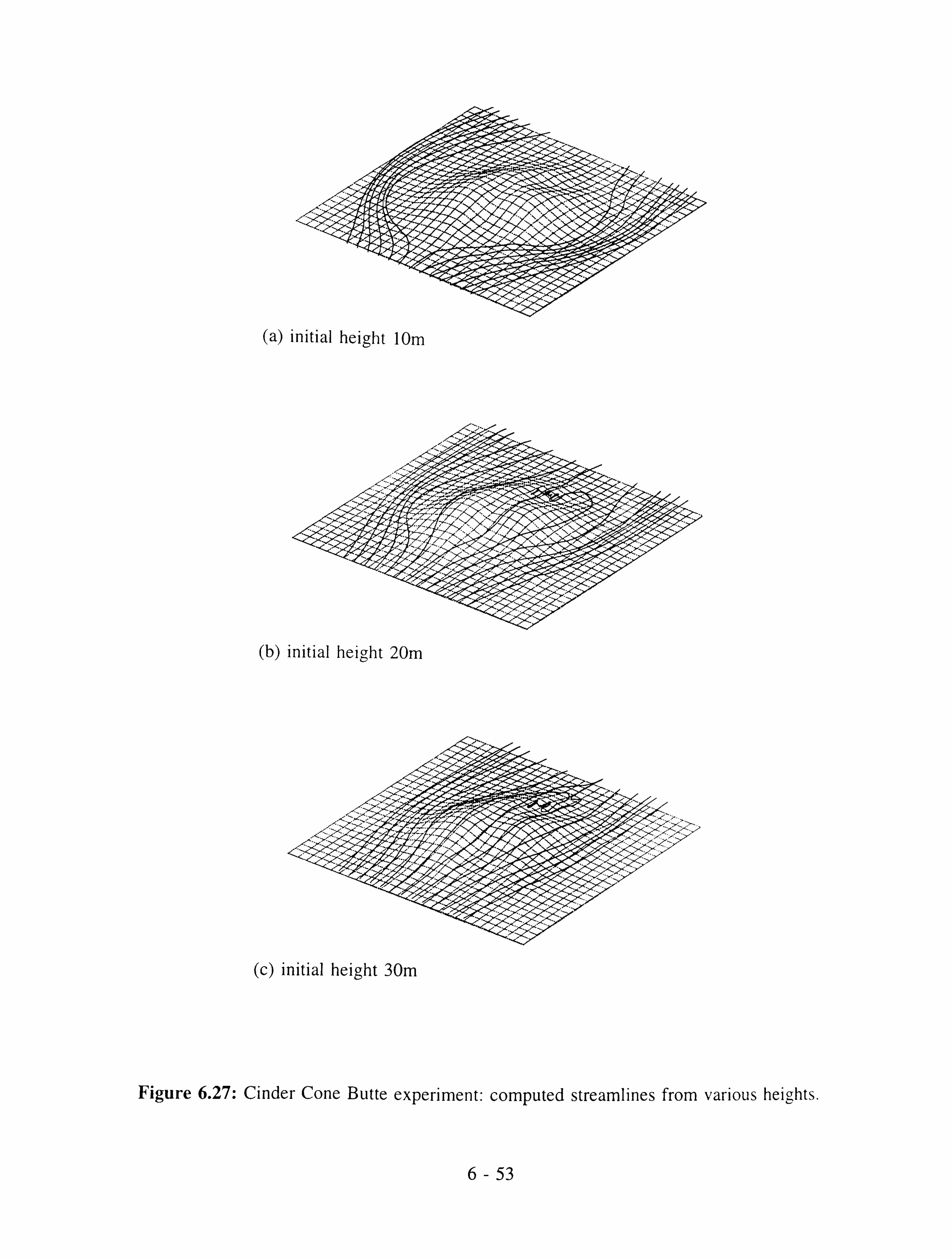
(a) initial height 10m

(b) initial height 20m

(c) initial height 30m

Figure 6.27: Cinder Cone Butte experiment: computed streamlines from various heights.

6-53

Figure 6.28: Cinder Cone Butte experiment: computed streamlines from the source location; initial vertical separation is 5m.

-1000 0 III

1000 2000 3000 4000

x (m)

(a) exponential potential temperature profile

0 ý

ý-'I

1000 2000 3000 4000

x (m)

(b) uniform potential temperature gradient

Figure 6.29: Cinder Cone Butte experiment: temperature isotherms computed over the Butte for different inflow stability types.

600

400

200

E ,.. T

-200

-400

-600

--------------

-- ----------- 7 77- -. - ----

=I rflflrt-t-HH--H-H

L li

I I1l11t7tttL- JtI1. H-. --. --4--. - ..,, .,. MIS Ims- Hill

;

------------- -------------------------- -------------------

-800 -600 -800

(a) flow grid

800

E ý

600

400

200

0 >1

-200

-400

-600

-800 -600 -800

-400

-400 -200 0 200 x (m)

(b) concentration grid

400 600 800

/

400 600 800

Figure 6.30: Cinder Cone Butte experiment: "flow" and "concentration" grids near the source.

-200 0 200 x (m)

6-56

600-1

400

200

E ý o.

>N

-200 -ý

-400 -1

source

-600 -800 -600 -400 -200 0 200 400 600 800

x (m)

(a) flow grid

600 -1

E ý >.

�

400-

200 -ý

o-

-200 -ý

--400-

source 0

-600 -800 -600 -400 -200 0 200

x (m)

(b) concentration grid

--T- 400 600 800

Figure 6.31: Cinder Cone Butte experiment: ground-level concentrations from flow and concentration grids.

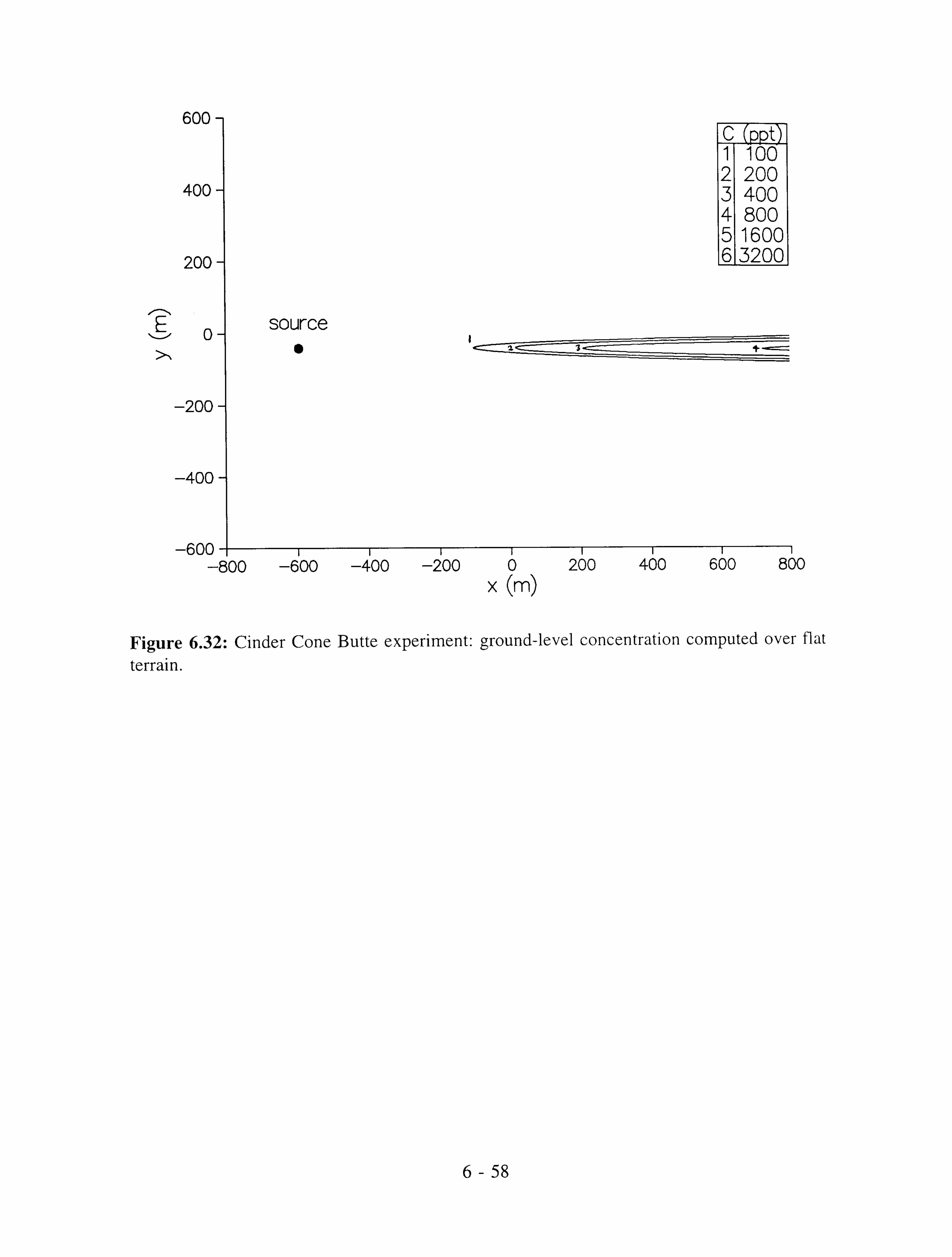
600 -1

>�

400 -I

200 -ý

source

Ct 1 100 2 200 3 400 4 800 5 1600 6 3200

ýPpt

1 ý23+

0

-200 -I

-400

-600 -800 -600 -400 -200 0 200 400 600 800

x (m)

Figure 6.32: Cinder Cone Butte experiment: ground-level concentration computed over flat

terrain.

C

2 3 4 5 6

100 200 400 800 1600 3200

400 -200 0 200 400

y (m)

Figure 6.33: Cinder Cone Butte experiment: vertical cross-section through the plume on the upwind slope of the Butte.

1 2 3 4 5

`ý ý

%

\\\

i/ \, ýý_--ý- \ ,%ýi,

/ý-- - ---ý\\'\ \ý /

,'//7 _-------ý_ \ýý. `. \

ý\ % // //

i/ 7 ---'-

`ýý \\ \,

\ ýN \

ý%; / /71' !0 \\ \ ýI//i , !i\ý !!; ýý ý_ ýý�ýýý ýý \ \

14It\\\ ý_ n _-

Jr1 AnM \. 1

ý760 xý j0

" -ý ý atl X11 ý :ý\//i ;1ý

source

ýý1 200 400 800 1600 3200

I

Figure 6.34: Cinder Cone Butte experiment: comparison of computed ground-level concentrations with hourly-averaged measurements, assuming a wind direction 127°. Only recorded concentrations above 200ppt are plotted.

Ct 1 100 2 200 3 400 4 800 5 1600 63200

Sarce --> "

(a) wind direction 127°

source

(b) wind direction 122°

sarce ý"

(c) wind direction 117°

Figure 6.35: Cinder Cone Butte experiment: sensitivity to approach-flow wind direction.

6-61

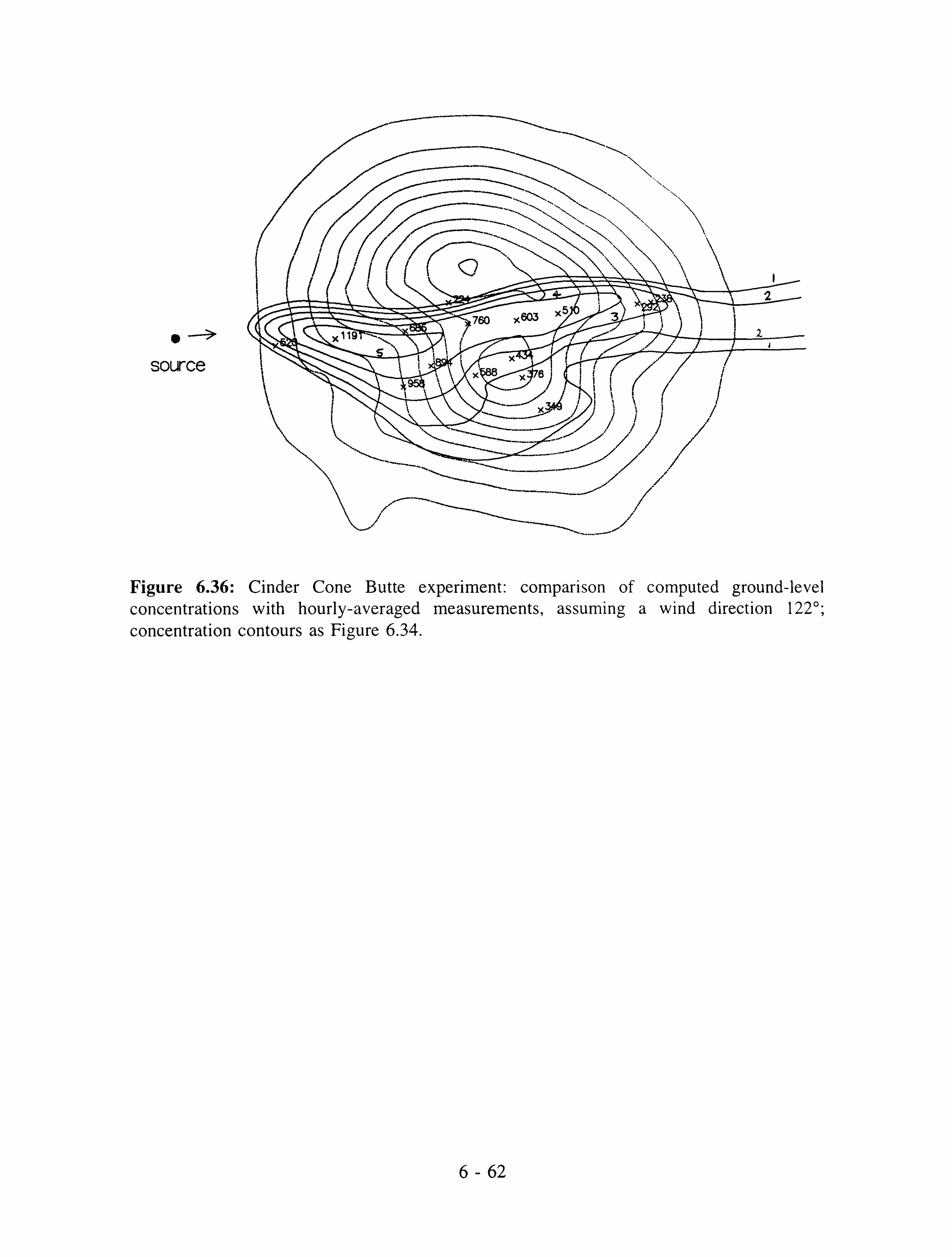
0 ---->

source

Figure 6.36: Cinder Cone Butte experiment: comparison of computed ground-level concentrations with hourly-averaged measurements, assuming a wind direction 122°; concentration contours as Figure 6.34.

3000

-ý--ý Q Q

ý N L- CL

0

2500

2000

1500

1000

500

I

500 1000 1500 2000 2500 3000 Cmeas (ppt)

Figure 6.37: Cinder Cone Butte experiment: scatter plot of observed vs predicted ground- level concentrations, assuming an approach-flow wind direction 122°.

CHAPTER 7.

Conclusions and Further Research

The various Chapters of this Thesis have covered: topographic effects on air flow and the

place of computational fluid dynamics in its modelling; a review of published literature and

related theory; the specification of a finite-volume computer code for predicting boundary-

layer flow and dispersion around topography; turbulence modelling and its application to the

atmospheric boundary layer; the comparison of numerical predictions with laboratory and field

measurements of flow and diffusion in complex terrain.

Whilst much of the material contained here relates to the implementation and assessment of

existing models, a number of original items have been included. A more formal treatment of

Leschziner and Rodi's (1981) modification to the k-c turbulence model to allow for mean-

streamline curvature is given, the geometric description in terms of spatial basis vectors

permitting a natural extension to three dimensions. A new "limited-length-scale k-c model"

is proposed, for flows (such as the atmospheric boundary layer) where the size of turbulent

eddies is limited by some external constraint - for example, stable stratification or the depth

of the turbulent layer. For dispersion calculations, it is shown how a region of analytically

specified concentrations may be imbedded within a finite-volume calculation to avoid the

necessity of focusing a highly refined grid near the source. The analytical concentration

distribution near the source is determined by the exact solution of a diffusion equation, which

avoids the singularity implied by gaussian-plume methods when the mean velocity is small

and along-wind diffusion is significant. Finally, the numerical product of this research - the

computer code SWIFT - has been assessed with respect to a number of hitherto untried

experimental datasets, including the very challenging test case of strongly stratified flow and

dispersion around three-dimensional real topography at Cinder Cone Butte.

Various levels of turbulence modelling have been reviewed. It is demonstrated that the

Coriolis and buoyancy forces occurring in atmospheric flows have strongly anisotropic effects

on the turbulent stresses. The cost and complexity of solving three-dimensional equations for

all second moments - in either their full stress-transport or algebraic stress closure forms - is

currently prohibitive for complex three-dimensional geometries and ha prompted a search for

(problem-specific) enhancements of simpler one- or two-equation turbulence models.

The standard two-equation k-E model is known to be inadequate in certain flows and

modifications to account for complex strains (streamline curvature and along-wind pressure

gradients) are described. These involve either a multiplying factor in the eddy-viscosity

coefficient linking turbulent stresses to mean strain, so as to enhance or diminish cross-stream

diffusion, or an adjustment to the balance of production and removal terms in the length-

scale-determining (dissipation) equation. Applications suggest that the latter approach (of

modifying the turbulent length scale) has a much greater impact on the overall flow structure

than the former (simplifying an algebraic stress model, which captures turbulence anisotropy).

Although demonstrated in an eddy-viscosity context, this has implications for more complex

second-order closure (Reynolds-stress transport) schemes, where attention has tended to be

focused on modelling the anisotropy-dependent pressure-strain (redistribution) at the expense

of the dissipation (removal) terms.

The strategy of adjusting the balance of production and removal terms in the dissipation

equation has been adopted for atmospheric boundary-layer simulations where the mixing

length is limited by some external constraint such as the depth of the turbulent layer or by

stable stratification. The new model, which simply increases the dissipation production term

as the mixing length approaches its externally-specified maximum, has some similarities to

that proposed by Detering and Etling (1985), but has the advantage of reducing to the

standard form, compatible with the logarithmic mean-velocity profile, near the surface. The

limited-length-scale k-c model has been successfully applied to predict the mean wind speed

profiles from the Leipzig experiment.

The modelling of a horizontally homogeneous, density stratified, Ekman layer is considered.

In the spirit of Nieuwstadt's (1984) model of an idealised stable boundary layer, a quasi-

steady state may be simulated in a boundary layer continually cooled from below by solving

for the potential-temperature difference between local height and the ground and transferring

the (constant) cooling rate to the source term. The result is a heat flux which varies linearly

with height up to the boundary-layer depth. The temperature jump at the top of the boundary

layer is, however, ill-defined. The approach has been combined with the limited-len-th-kale k-£ model described above to compute mean wind and temperature profiles measured at the UK Meteorological Office's Cardington field site, with moderate success.

The code SWIFT - Stratified WInd Flow over Topography - is a three-dimensional, finite-

volume, incompressible flow solver, using a terrain-following, non-orthogonal coordinate mesh to compute turbulent flow over arbitrary smooth topography. The code uses a Cartesian velocity decomposition (which allows the curvilinear equations of motion to be framed in

conservative form) and a staggered velocity grid. Provided the mesh distortion from Cartesian is not too great (so that coordinate-wise pressure gradients drive the intermediate velocity

component) this latter arrangement not only eliminates the well-known problem of odd-even

pressure-node decoupling but permits the use of pressure-correction algorithms which are

considerably more efficient than the original SIMPLE scheme. A number of SIMPLE-like

variants have been coded in SWIFT, the most effective of which is SIMPLEX (Raithby and

Schneider, 1988), which obtains a more accurate relationship between velocity and pressure

corrections by solving equations for the connecting coefficients. The solution of the pressure-

correction equation occupies a substantial proportion of the overall computing time and two

schemes - the block-correction method of Patankar (1988) and the anticipated-correction

scheme of Van Doormaal and Raithby (1984) - have been found particularly beneficial in

reducing this overhead, whilst still remaining within the line-iterative matrix solution method

common to TEACH-like codes. The first acceleration technique involves preceding the

directional sweeps by adding block corrections satisfying the integral equations derived by

summing coefficients over the normal directions. In some senses it is a very coarse form of

the multigrid technique. The second method tries to minimise the error involved in the

directional pass through the mesh lines by anticipating the change in variables on lines not

yet updated.

Turbulence modelling and numerical solution have been used in a combined assault on two

test cases of flow and dispersion over complex terrain. The first is the RUSHIL experiment

of Khurshudyan et al. (1981), involving wind-tunnel measurements of (unstratified) flow and

dispersion over two-dimensional model hills. The second is a particular case-study hour of

dispersion in strongly stratified flow at Cinder Cone Butte in Idaho, USA (Lavery et al.,

1982).

Mean-flow predictions for the RUSHIL experiment were generally in line with the experimental data, confirming lee-side separation for the steepest hill, but not for that of least slope. In some respects, the intermediate-slope case was the most challenging, since intermittent separation was observed in the wind tunnel -a feature not strictly resolvable by the time-averaged system of equations used here. This had considerable impact on the concentration distribution since, in the wind tunnel, material was intermittently entrained into

recirculating flow. Variations on a k-£-turbulence-model theme were made for streamwie pressure gradients and streamline curvature. The first greatly improved mean-flow predictions in the separation region. The second had little impact on the mean flow although it produced slightly better turbulence energy profiles. The turbulent kinetic energy was, however,

generally underpredicted by all turbulence model variants.

Concentration calculations represent more of a challenge for turbulence modelling because

it is the velocity fluctuations which are responsible for relative dispersion and dilution of

plume material. Isotropic eddy-viscosity models (such as k-E) generally provide a good

representation of the mean flow in simple shear layers because only the shear stresses appear in the Reynolds-averaged momentum equation. On the other hand, in such flows these models

predict that all norinal stresses are equal (to 2k/3), in contradiction of experiment. In the

atmospheric boundary layer, lateral spread generally exceeds that in the vertical because

vertical fluctuations are damped by the ground (and by stable stratification). Lateral spread

may also be a strong function of averaging time. In simulations of plume dispersion in the

RUSHIL experiment the computations underpredicted lateral spread. However, this deficiency

could be offset by normalising on the maximum ground-level concentration in the absence

of the hill, whereby very good agreement for "terrain amplification factors" was obtained. For

the case of steady flow separation the impact of the recirculating-flow region was well-

predicted. However, some deficiencies were observed for the case of intermittent separation,

since the time-averaged flow equations failed to recognise any period of reversed flow.

The Cinder Cone Butte dispersion study represented a very challenging test case because of

the (not unrelated) effects of strong stratification and sensitivity to wind direction. The

7-4

(stability-dependent) limited-length-scale strategy was adopted in the turbulence closure: without it the k-c turbulence model created too much diffusion and lamely eroded the

approach-flow temperature profile. Although detailed flow measurements were not documented in the accounts of the field (or laboratory) experiments a number of qualitative flow features - such as the separated-flow region in the wake - were faithfully reproduced in

the numerical computations.

Conclusions drawn from the flow and dispersion simulations of the Cinder Cone Butte

experiment have important implications for dispersion modelling practice in strongly stratified flow around topography. Among them we may list the following.

Dividing-streamline concept. Calculations indicate that strong stratification does

compel the fluid at lower levels to move in roughly parallel planes around the

hill. However, the depth of this layer is less than that suggested by the

dividing-streamline height calculated from the approach-flow stability profile.

Computations of streamline behaviour suggest that the concept of a sharp

transition from horizontal potential flow to near-neutral flow above is rather

naive.

Strong vertical wind shear. Very stable density gradients cause significant lateral deviation

near the ground with weaker displacement aloft. In consequence the crosswind profile

through the plume is strongly skewed.

Sensitivity to wind direction. In very stable flow the concentration plume can switch from one

side of a hill to the other for very small changes in wind direction. In consequence the

time-averaged lateral spread can be substantially higher - and ground-level

concentrations much lower - than suggested by the angular variation in the approach-

flow wind direction and the time-averaged mean flow. Although there was very little

prospect of determining this from the full-scale experiments, computations of the

wind-direction dependence on plume dispersion were in very good agreement with the

laboratory towing tank experiments of Snyder and Lawson (1981).

Plume impingement. For low-level sources the highest ground-level concentration: occur when the horizontal distance to the hill surface is smallest.

Non-ideal topography. Wind-field calculations demonstrate that strong stability enhance the lateral asymmetry associated with the detailed shape of the hill, belying the common practice of idealising topography as simple axisymmetric shapes for dispersion

calculations. The possibility of advection into a three-dimensional recirculation zone on the lee slope may lead to enhanced ground-level concentrations on that side of the hill.

Narrow plume assumption. As a combination of the effects listed above the assumption of a

plume of gaussian (or any other specified) profile, with dispersion characteristics

governed by conditions on the plume centreline, is untenable.

Thus concludes a theoretical and numerical study of flow and diffusion around topography.

There is much scope for further work. Although the prediction of flow around three-

dimensional real topography has been demonstrated, it is computationally demanding and the

routine application of the model to real terrain would benefit from further improvement to the

numerics. Multigrid, multiblock and local-mesh-refinement capabilities would all be beneficial

in this respect. Some theoretical discussion of the hydrostatic approximation has been given

here and it would be interesting to incorporate this as an option within SWIFT to investigate

the range of validity of the approximation. In dispersion calculations it has been seen how

isotropic eddy-diffusivity models tend to underestimate lateral dispersion and the inclusion

of an anisotropic eddy-diffusivity tensor for concentration calculations would make a

worthwhile project.

Finally, a perspective. How far have we come with the computational modelling of complex

environmental flows? In his far-sighted book "Weather Prediction By Numerical Processes"

L. F. Richardson (1922) founded the modern science of numerical weather forecasting: albeit

7-6

with a (conservative) estimate of 64000 human computers to solve the dikcreti`ed equation, for the whole globe. In it he describes his whimsical fantasy of a "forecast factory", which we make no apologies for quoting in its entirety:

Imagine a large hall like a theatre, except that the circles and galleries go right round through the space usually occupied by the stage. The walls of this chamber are painted to form a map of the globe. The ceiling represents the north-polar regions, England is in the gallery, the tropics in the upper circle, Australia on the dress circle and the antarctic in the pit. A myriad computers are at work upon the weather of the part of the map wherc each sits, but each computer attends only to one equation or part of an equation. The work of each region is coordinated by an official of higher rank. Numerous little "night signs" display the instantaneous values so that neighbouring computers can read them. Each number is thus displayed in three adjacent ; ones so as to maintain communication to the North and South on the map. From the floor of the pit a tall pillar rises to half the height of the hall. It carries a large pulpit oil its top. In this sits the man in charge of the %''hole theatre; he is surrounded by several assistants and messengers. One of his duties is to maintain a uniform speed of progress in all parts of the globe. In this respect he is like the conductor of an orchestra in which the instruments are slide- rules and calculating machines. But instead of waving a baton he turns a beam of rosy light upon any region which is running ahead of the rest, and a beam of blue light upon those who are behindhand.

Four senior clerks in the central pulpit are collecting the fixture weather as fast as it is being computed, and dispatching it by pneumatic carrier to a quiet room. There it will be coded and telephoned to the radio transmitting station.

Messengers carn y piles of used computer forms down to a storehouse in the cellar.

In a neighbouring building there is a research department, where they invent improvements. But there is much experimenting on a small scale before any change is made in the complex routine of the computing theatre. In a basement an enthusiast is observing eddies in the liquid lining of a huge spinning bowl, but so far the arithmetic proves the better way. In another building are all the usual financial, correspondence and administrative offices

But before we indulge in a smug smile at a fantasy long since surpassed -

... Outside are playing fields, houses, mountains and lakes, for it was thought

that those who compute the weather should breathe of it freely.

Maybe Richardson had it right after all!

Bibliography

Apsley, D. D., 1988, A model for dispersion in the wake of large buildings. CEGB Report RD/L/3359/R88

Arya, S. P. S., 1982, Atmospheric boundary layers over homogeneous terrain, Chapter 6 in Engineering Meteorology, Plate, E. (ed. ), Elsevier

Arya, S. P. S. and Gadiyaram, P. S., 1986, An experimental study of flow and dispersion in the

wakes of three-dimensional low hills, Atmospheric Environment, 20,729-740

Arya, S. P. S. and Shipman, M. S., 1981, An experimental investigation of flow and diffusion

in the disturbed boundary-layer flow over a ridge - I. Mean flow and turbulence structure, Atmospheric Environment, 15,1173-1184

Arya, S. P. S., Shipman, M. S. and Courtney, L. Y., 1981, An experimental investigation of flow

and diffusion in the disturbed boundary-layer flow over a ridge - II. Diffusion from a

continuous point source, Atmospheric Environment, 15,1185-1194

Bacmeister, J. T. and Pierrehumbert, R. T., 1988, On high-drag states of non-linear stratified

flow over an obstacle, Journal of the Atmospheric Sciences, 45,63-80

Baines, P. G. and Hoinka, K. P., 1985, Stratified flow over two-dimensional topography in fluid

of infinite depth: a laboratory simulation, Journal of the Atmospheric Sciences, 42,1614-1630

Baines, P. G. and Manins, P. C., 1989, The principles of laboratory modelling of stratified

atmospheric flows over complex terrain, Journal of Applied Meteorology, 28,1213-1225

Belcher, S. E., Xu, D. P. and Hunt, J. C. R., 1990, The response of a turbulent boundary-layer

to arbitrarily distributed two-dimensional roughness changes, Quarterly Journal of the Royal

Meteorological Society, 611-635

B-1

Beljaars, A. C. M., Walmsley, J. L. and Taylor, P. A., 1987, A mixed spectral finite-difference

model for neutrally-stratified boundary layer flow over roughness changes and topography. Boundary layer meteorology, 38,273-303

Blackadar, A. K., 1962, The vertical distribution of wind and turbulent exchange in a neutral

atmosphere, Journal of Geophysical Research, 97,3095-3102

Bowen, A. J. and Lindley, D., 1977, A wind tunnel investigation of the wind speed and

turbulence characteristics close to the ground over various escarpment shapes, Boundary-Layer

Meteorology, 12,259-271

Bradley, E. F., 1980, An experimental study of the profiles of wind speed, shearing stress and

turbulence at the crest of a large hill, Quarterly Journal of the Royal Meteorological Society,

106,101-123

Bradley, E. F., 1983, The influence of thermal stability and angle of incidence on the

acceleration of wind up a slope, Journal of Wind Engineering and Industrial Aerodynamics,

15,231-242

Bradshaw, P., 1969, The analogy between streamline curvature and buoyancy in turbulent

shear flow, Journal of Fluid Mechanics, 36,177-191

Brighton, P. W. M., 1978, Strongly stratified flow past three-dimensional obstacles, Quarterly

Journal of the Royal Meteorological Society, 104,289-307

Britter, R. E., Hunt, J. C. R. and Richards, K. J., 1981, Air flow over a two-dimensional hill:

studies of velocity speed-up, roughness effects and turbulence, Quarterly Journal of the Royal

Meteorological Society, 107,91-110

Brost, R. A. and Wyngaard, J. C., 1978, A model study of the stably-stratified planetary

boundary layer, Journal of the Atmospheric Sciences, 35,1427-1440

B-2

Brunt, D., 1927, The period of simple vertical oscillations in the atmosphere, Quarterle


Burt, E. W., 1977, VALLEY User's Guide, United States Environmental Protection Agency

report EPA-450/2-77-018

Carruthers, D. J., Hunt, J. C. R., Britter, R. E., Perkins, R. J., Linden, P. F. and Dalziel, S., 1991,

Fast models on small computers of turbulent flows in the environment for non-expert users,

in Computer Modelling in the Environmental Sciences, Farmer, D. G. and Rycroft, M. J., (eds. ),

Clarendon Press, Oxford

Castro, I. P., 1987, A note on lee wave structures in stratified flow over three-dimensional

obstacles, Tellus, 39A, 72-81

Castro, I. P. and Robins, A. G., 1993, The National Power Environmental Flow Research

Centre, University of Surrey Mechanical Engineering Department Report ME-FD/93.15

Castro, I. P. and Snyder, W. H., 1982, A wind tunnel study of dispersion from sources

downwind of three-dimensional hills, Atmospheric Environment, 16,1869-1887

Castro, I. P. and Snyder, W. H., 1993, Experiments on wave breaking in stratified flow over

obstacles, Journal of Fluid Mechanics, 255,195-211

Castro, I. P., Snyder, W. H. and Lawson, R. E., 1988, Wind direction effects on dispersion from

sources downwind of steep hills, Atmospheric Environment, 22,2229-2238

Castro, I. P., Snyder, W. H. and Marsh, G. L., 1983, Stratified flow over three-dimensional

ridges, Journal of Fluid Mechanics, 135,261-282

Chien, K. -Y., 1982, Predictions of channel and boundary-layer flows with a low-Reynolds-

number turbulence model, AIAA Journal, 20,33-38

B-3

Clark, T. L., 1977, A small-scale dynamic model using a terrain following coordinate transformation, Journal of Computational Physics, 24,186-215

Clark, T. L. and Peltier, W. R., 1977, On the evolution and stability of finite amplitude

mountain waves, Journal of the Atmospheric Sciences, 34,1715-1730

Clark, T. L. and Peltier, W. R., 1984, Critical level reflection and the resonant growth of non- linear mountain waves, Journal of the Atmospheric Sciences, 41,3122-3134

Clarke, R. H., 1979, First report of a working group on atmospheric dispersion: A model for

short and medium range dispersion of radionuclides released to the atmosphere, National

Radiological Protection Board report NRPB-R91

Coleman, G. N., Ferziger, J. H. and Spalart, P. R., 1990, Direct simulation of the turbulent

Ekman layer, Journal of Fluid Mechanics, 213,313-348

Coleman, G. N., Ferziger, J. H. and Spalart, P. R., 1992, Direct simulation of the stably

stratified turbulent Ekman layer, Journal of Fluid Mechanics, 244,677-712

Coppin, P. A., Bradley, E. F. and Finnigan, J. J., 1994, Measurements of flow over an elongated

ridge and its stability dependence: the mean field, Boundary Layer Meteorology, 69,173-199

Crapper, G. D., 1959, A three-dimensional solution for waves in the lee of mountains, Journal

of Fluid Mechanics, 6,51-76

Dawson, P., Stock, D. E. and Lamb, B., 1991, The numerical simulation of airflow and

dispersion in three-dimensional atmospheric recirculation zones, Journal of Applied


Deaves, D. M., 1976, Wind over hills: a numerical approach, Quarterly Journal of the Royal


B-4

Deaves, D. M., 1980, Computations of wind flow over two-dimensional hills and embankments, Journal of Wind Engineering and Industrial Aerodynamics, 6,89-111

Defant, F., 1951, Local Winds, Compendium of Meteorology, Malone, T. J.. Ed.. American Meteorological Society, 655-675

Derbyshire, S. H., 1990, Nieuwstadt's stable boundary layer revisited, Quarterly Journal of the Royal Meteorological Society, 116,127-158

Desiato, F., 1991, A dispersion model evaluation study for real-time application in complex

terrain, Journal of Applied Meteorology, 30,1207-1219

Detering, H. W. and Etling, D., 1985, Application of the E-e turbulence model to the

atmospheric boundary-layer, Boundary-Layer Meteorology, 33,113-133

Drazin, P. G., 1961, On the steady flow of a fluid of variable density past an obstacle, Tellus,

13,239-251

Durran, D. R. and Klemp, J. B., 1987, Another look at downslope winds. Part II: Non-linear

amplification beneath wave-overturning layers, Journal of the Atmospheric Sciences, 44,

3402-3412

Egan, B. A., 1975, Turbulent diffusion in complex terrain, Lectures on Air Pollution and

Environmental Impact Analyses, American Meteorological Society, Boston, Mass., 112-135

Egan, B. A., 1984, Transport and diffusion in complex terrain, Boundary Layer Meteorology,

30,3-28

Ekman, V. W., 1904, On dead water, Scientific Results of the Norwegian North Polar

Expedition, 5, No. 15,1-152

Ekman, V. W., 1905, On the influence of the earth's rotation on ocean currents, Arkiv Mat.

B-5

Astron. Fysik, 2(11)

El Tahry, S., Gosman, A. D. and Launder, 1981, The two- and three-dimensional dispersal of

a passive scalar in a turbulent boundary-layer, International Journal of Heat and Mass

Transfer, 24,35-46

Fackrell, J. E., 1984, Parameters characterising dispersion in the near wake of buildings,

Journal of Wind Engineering and Industrial Aerodynamics, 16,97-118

Garratt, J. R., 1992, The Atmospheric Boundary Layer, Cambridge University Press

Gaskell, P. H. and Lau, A. K. C., 1988, Curvature-compensated convective transport: SMART,

a new boundedness-preserving transport algorithm, International Journal For Numerical

Methods in Fluids, 8,617-641

Gibson, M. M. and Launder, B. E., 1976, On the calculation of horizontal, turbulent, free shear

flows under gravitational influence, Journal of Heat Transfer, 98,81-87

Gill, A. E., 1982, Atmosphere-Ocean Dynamics, Academic Press

Gong, W., 1991, A wind tunnel study of turbulent dispersion over two- and three-dimensional

gentle hills from upwind point sources in neutral flow, Boundary-Layer Meteorology, 54,211-

230

Gong, W. and Ibbetson, A., 1989, A wind tunnel study of turbulent flow over model hills,

Boundary-Layer Meteorology, 49,113-148

Gryning, S. E., Holtslag, A. A. M., Irwin, J. S. and Sivertsen, B., 1987, Applied dispersion

modelling based on meteorological scaling parameters, Atmospheric Environment, 21,79-89

Han, T. Y., Meng, J. C. S. and Innis, G. E., 1983, An open boundary condition for

incompressible stratified flows, Journal of Computational Physics, 49,276-297

B-6

Hanjalic, K., 1994, Advanced turbulence closure models: a view of current status and future

prospects, International Journal of Heat and Fluid Flow, 15,178-203

Hanjalic, K. and Launder, B. E., 1980, Sensitising the dissipation equation to irrotational

strains, Journal of Fluids Engineering, 102,34-40

Harlow, F. H. and Welch, J. E., 1965, Numerical calculation of time-dependent viscous incompressible flow of fluid with a free surface, Physics of Fluids, 8,2182-2189

Heilman, W. E. and Takle, E. S., 1991, Numerical simulation of the nocturnal turbulence

characteristics over Rattlesnake Mountain, Journal of Applied Meteorology, 30,1106-1116

Holtslag, A. A. M. and Nieuwstadt, F. T. M., 1986, Scaling the atmospheric boundary layer,


Howard, L. N., 1961, Note on a paper of John W. Miles, Journal of Fluid Mechanics, 10,509-

512

Hunt, J. C. R., Abell, C. J., Peterka, J. A. and Woo, H., 1978, Kinematical studies of the flows

around free or surface-mounted obstacles; applying topology to flow visualisation, Journal of

Fluid Mechanics, 86,179-200

Hunt, J. C. R., Holroyd, R. H., Carruthers, D. J., Robins, A. G., Apsley, D. D., Smith. F. B. and

Thomson, D. J., 1990, Developments in modelling air pollution for regulatory uses, 18`h

NATO-CCMS International Conference on Air Pollution Modelling and its Applications,

Vancouver, Canada

Hunt, J. C. R., Kaimal, J. C. and Gaynor, J. E., 1985, Some observations of turbulence structure

in stable layers, Quarterly Journal of the Royal Meteorological Society, 111,793-815

Hunt, J. C. R., Leibovich, S. and Richards, K. J., 1988a, Turbulent shear flow over low hills.

Quarterly Journal of the Royal Meteorological Society, 114,1435-1470

B-7

Hunt, J. C. R., Richards, K. J. and Brighton, P. W. M., 1988b, Stably stratified shear flow over low hills, Quarterly Journal of the Royal Meteorological Society, 114.859-886

Hunt, J. C. R., Puttock, J. S. and Snyder, W. H., 1979, Turbulent diffusion from a point source in stratified and neutral flows around a three-dimensional hill - Part I. Diffusion equation

analysis, Atmospheric Environment, 13,1227-1239

Hunt, J. C. R. and Snyder, W. H., 1980, Experiments on stably and neutrally stratified flow over

a model three-dimensional hill, Journal of Fluid Mechanics, 96,671-704

Hunt, J. C. R., Spalart, P. and Mansour, N., 1987, A general form for the dissipation length

scale in turbulent shear flows, Proceedings of the 1st Summer Program NASA/Stanford Center

For Turbulence Research

Huppert, H. E. and Miles, J. W., 1969, Lee waves in a stratified flow. Part 3. Semi-elliptical

obstacle, Journal of Fluid Mechanics, 35,497-525

Issa, R. I., 1985, Solution of the implicitly discretised fluid flow equations by operator-

splitting, Journal of Computational Physics, 62,40-65

Jackson, P. S. and Hunt, J. C. R., 1975, Turbulent wind flow over a low hill, Quarterly Journal

of the Royal Meteorological Society, 101,929-955

Janowitz, G. S., 1984, Lee waves in three-dimensional stratified flow, Journal of Fluid

Mechanics, 148,97-108

Jenkins, G. J., Mason, P. J., Moores, W. H. and Sykes, R. I., 1981, Measurements of the flow

structure around Ailsa Craig, a steep, three-dimensional, isolated hill, Quarterly Journal of the

Royal Meteorological Society, 107,833-851

Jones, J. A., 1986, Seventh report of a working group on atmospheric dispersion: The

uncertainty in dispersion estimates obtained from the working group models, National

B-8

Radiological Protection Board report NRPB-R 199

Keller, T. L., 1994, Implications of the hydrostatic assumption on atmospheric gravity waves. Journal of the Atmospheric Sciences, 51,1915-1929

Khurshudyan, L. H., Snyder, W. H. and Nekrasov, IN., 1981, Flow and dispersion of pollutants

over two-dimensional hills, United States Environmental Protection Agency Report EPA-

600/4-81-067

Kitabayashi, K., 1991, Wind tunnel simulation of airflow and pollutant diffusion over

complex terrain, Atmospheric Environment, 25A, 1155-1161

Klemp, J. B. and Durran, D. R., 1983, An upper boundary condition permitting internal gravity

wave radiation in numerical mesoscale models, Monthly Weather Review, 111,430-444

Lam, C. K. G. and Bremhorst, K. A., 1981, Modified form of the k-E model for predicting wall

turbulence, Journal of Fluids Engineering, 103,456-460

Launder, B. E., 1988, On the computation of convective heat transfer in complex turbulent

flows, Journal of Heat Transfer, 110,1112-1128

Launder, B. E., 1989, Second-Moment Closure: present... and future?, International Journal of

Heat and Fluid Flow, 10,282-300

Launder, B. E. and Sharma, B. I., 1974, Application of the energy-dissipation model of

turbulence to the calculation of flow near a spinning disc, Letters in Heat and Mass Transfer,

1,131-138

Launder, B. E. and Spalding, D. B., 1974, The numerical computation of turbulent flows,

Computer Methods in Applied Mechanics and Engineering, 3,269-289

Lavery, T. F., Bass, A., Strimaitis, D. G., Venkatram, A., Green B. R. and Drivas, P. J.. 1982.

B-9

EPA Complex Terrain Model Development: First Milestone Report. US Environmental Protection Agency Report EPA-600/3-82-036

Leonard, B. P., 1979, A stable and accurate convective modelling procedure based on quadratic upstream interpolation, Computational Methods in Applied Mechanical Engineering. 19,59-98

Leonard, B. P. and Mokhtari, S., 1990, Beyond first-order upwinding: the ULTRA-SHARP

alternative for non-oscillatory steady-state simulation of convection, International Journal for

Numerical Methods in Engineering, 30,729-766

Leschziner, M. A. and Rodi, W., 1981, Calculation of annular and twin parallel jets using

various discretisation schemes and turbulence-model variations, Journal of Fluids Engineering,

103,352-360

Lettau, H., 1950, A re-examination of the 'Leipzig wind profile' considering some relations

between wind and turbulence in the friction layer, Tellus, 2,125-129

Lien, F. -S., 1992, Computational modelling of 3D flow in complex ducts and passages, PhD

Thesis, UMIST

Lien, F. -S. and Leschziner, M. A., 1993, UMIST Department of Mechanical Engineering

Report TFD/93/12

Lien, F. -S. and Leschziner, 1993, A pressure-velocity solution strategy for compressible flow

and its application to shock/boundary-layer interaction using second-moment turbulence

closure, Journal of Fluids Engineering, 115,717-725

Lighthill, J., 1978, Waves in Fluids, Cambridge University Press

Lillington, J. N., 1981, A vector upstream differencing scheme for problems in fluid flow

involving significant source terms in steady-state linear systems, International Journal of

B-10

Numerical Methods in Fluids, 1,3-16

Long, R. R., 1952, Some aspects of the flow of stratified fluids I. a theoretical investigation, Tellus, 5,42-58

Lyra, G., 1943, Theorie der stationären Leewellenstromung in freier Atmosphäre, Z. Angew. Math. Mech., 23,1-28

Majumdar, S., Rodi, W. and Zhu, J., 1992, Three-dimensional finite volume method for incompressible flows with complex boundaries, Journal of Fluids Engineering, 114,496-503

Maryon, R. H., Whitlock, J. B. G. and Jenkins, G. J., 1986, An analysis of short-range dispersion

experiments on the windward slope of an isolated hill, Atmospheric Environment, 20,2157- 2173

Mason, P. J., 1986, Flow over the summit of an isolated hill, Boundary Layer Meteorology,

37,385-405

Mason, P. J., 1989, Large-eddy simulation of the convective atmospheric boundary layer,

Journal of the Atmospheric Sciences, 46,1492-1516

Mason, P. J. and Derbyshire, S. H., 1990, Large-eddy simulation of the stably-stratified

atmospheric boundary layer, Boundary layer Meteorology, 53,117-162

Mason, P. J. and King, J. C., 1985, Measurements and predictions of flow and turbulence over

an isolated hill of moderate slope, Quarterly Journal of the Royal Meteorological Society, 111,

617-640

Mason, P. J. and Sykes, R. I., 1979a, Flow over an isolated hill of moderate slope, Quarterly


Mason, P. J. and Sykes, R. I., 1979b, Three-dimensional numerical integrations of the Navier-

B-11

Stokes equations for flow over surface-mounted obstacles, Journal of Fluid Mechanics, 91. 433-450

Mason, P. J. and Sykes, R. I., 1981, On the influence of topography on plume dispersal, Boundary Layer Meteorology, 21,137-157

Mason, P. J. and Thomson, D. J., 1987, Large-eddy simulation of the neutral-static-stability

planetary boundary layer, Quarterly Journal of the Royal Meteorological Society, 113,413-

443

McIntyre, M. E., 1972, On Long's Hypothesis of no upstream influence in uniformly stratified

or rotating flow, Journal of Fluid Mechanics, 52,209-243

McNider, R. T. and Pielke, R. A., 1984, Numerical simulation of slope and mountain flows,

Journal of Climate and Applied Meteorology, 23,1441-1453

Mellor, G. L. and Yamada, T., 1974, A hierarchy of turbulence closure models for planetary

boundary layers, Journal of the Atmospheric Sciences, 31,1791-1806

Mellor, G. L. and Yamada, T., 1982, Development of a turbulence closure model for

geophysical fluid problems, Reviews of Geophysics and Space Physics, 20,851-875

Mickle, R. E., Cook, N. J., Hoff, A. M., Jensen, N. O., Salmon, J. R., Taylor, P. A., Tetzlaff, G.

and Teunissen, H. W., 1988, The Askervein hill project: vertical profiles of wind and

turbulence, Boundary-Layer Meteorology, 43,143-169

Miles, J. W., 1961, On the stability of heterogeneous shear flows, Journal of Fluid Mechanics,

10,496-508

Miller, M. J. and Thorpe, A. J., 1981, Radiation conditions for the lateral boundaries of limited-

area numerical models, Quarterly journal of the Royal Meteorological Society, 107,615-628

B-12

Miranda, P. M. A. and James, I. N., 1992, Non-linear three-dimensional effects on gravity-wave drag: splitting flow and breaking waves, Quarterly Journal of the Royal Meteorological Society, 118,1057-1081

Mylne, B. and Callander, B. A., 1989, Short range tracer dispersion experiments at Nyland Hill, Atmospheric Environment, 23,2667-2677

Neal, D., 1983, The influence of model scale on a wind tunnel simulation of complex terrain, Journal of Wind Engineering and Industrial Aerodynamics, 12,125-143

Nieuwstadt, F. T. M., 1984, The turbulent structure of the stable nocturnal boundary layer.


Nieuwstadt, F. T. M., 1985, A model for the stationary, stable boundary layer, Proc. of IMA

conference on turbulence and diffusion in the stable environment, Cambridge, 1983, Hunt,

J. C. R. (ed. ), Clarendon Press

Nieuwstadt, F. T. M. and van Harem, L., 1988, A large eddy simulation of buoyant and non-

buoyant plume dispersion in the convective atmospheric boundary layer, in Air Pollution

Modelling and its Applications, van Dop, H. (ed. ), Plenum

Orlanski, I., 1976, A simple boundary condition for unbounded hyperbolic flows, Journal of

Computational Physics, 21,251-269

Pasquill, F. and Smith, F. B., 1983, Atmospheric Diffusion, Ellis-Horwood

Patankar, S. V., 1980, Numerical Heat Transfer and Fluid Flow, McGraw-Hill

Patankar, S. V., 1988, Elliptic systems: finite difference method I, Chapter 6 in Handbook of

Numerical Heat Transfer, Minkowycz, W. J., Sparrow, E. M., Schneider, G. E. and Pletcher,

R. H. (eds. ), Wiley

B-13

Patel, V. C., Rodi, W. and Scheurer, G., 1985, Turbulence models for near-wall and low Reynolds number flows: a review, AIAA Journal, 23,1308-1319

Pearse, J. R., 1982, Wind flow over conical hills in a simulated atmospheric boundary laver. Journal of Wind Engineering and Industrial Aerodynamics, 10,303-313

Pearse, J. R., Lindley, D. and Stevenson, D. C., 1981, Wind flow over ridges in simulated atmospheric boundary layers, Boundary-Layer Meteorology, 21,77-92

Pearson, H. J., Puttock, J. S. and Hunt, J. C. R., 1983, A statistical model of fluid-element

motions and vertical diffusion in a homogeneous stratified turbulent flow, Journal of Fluid


Perry, S. G., 1992, CTDMPLUS: A dispersion model for sources near complex topography.

Part I: Technical Formulations, Journal of Applied Meteorology, 31,633-660

Puttock, J. S. and Hunt, J. C. R., 1979, Turbulent diffusion from sources near obstacles with

separated wakes - Part I. An eddy diffusivity model, Atmospheric Environment, 13,1-13

Queney, P., 1948, The problem of air flow over mountains: a summary of theoretical studies,

Bulletin of the American Meteorological Society, 29,16-26

Raithby, G. D., 1976, Skew upstream differencing schemes for problems involving fluid flow,

Computer Methods in Applied Mechanics and Engineering, 9,153-164

Raithby, G. D. and Schneider, G. E., 1988, Elliptic systems: finite difference method II,

Chapter 7 in Handbook of Numerical Heat Transfer, Minkowycz, W. J., Sparrow, E. M.,

Schneider, G. E. and Pletcher, R. H. (eds. ), Wiley

Raithby, G. D., Stubley, G. D. and Taylor, P. A., 1987, The Askervein hill project: a finite

control volume prediction of three-dimensional flows over the hill, Boundary-Layer


B-14

Rau, M., Bächlin, W. and Plate, E. J., 1991, Detailed design features of a new wind tunnel for

studying the effects of thermal stratification, Atmospheric Environment, 25A. 1257-1262

Rayleigh, Lord, 1880, On the stability, or instability, of certain fluid motions, Proceedings of the London Mathematical Society, 9,57-70

Rayleigh, Lord, 1883, Investigation of the character of the equilibrium of an incompressible

heavy fluid of variable density, Proceedings of the London Mathematical Society, 14,170-177

Rhie, C. M. and Chow, W. L., 1983, A numerical study of the turbulent flow past an isolated

airfoil with trailing edge separation, AIAA Journal, 21,1525-1532

Richardson, L. F., 1922, Weather Prediction by Numerical Processes, Cambridge University

Press

Robins, A. G., 1977, The development and structure of simulated neutrally stable atmospheric

boundary layers, CEGB Report R/M/R246

Robins, A. G., 1983, Recent advances in the modelling of dispersion near buildings, Proc. Inst.

Mech. Eng. Conference on Heat and Fluid Flow in Nuclear and Process Plant Saftey, 49-56

Rodi, W., 1985, Calculation of stably stratified shear-layer flows with a buoyancy-extended

k-E model, in Turbulence and Diffusion in the Stable Environment, Hunt, J. C. R. (ed. ), 111-

143, Oxford University Press

Rodi, W., 1987, Examples of calculation methods for flow and mixing in stratified fluids,

Journal of Geophysical Research, 92,5305-5328

Rodi, W. and Mansour, N. N., 1993, Low Reynolds number k-c modelling with the aid of

direct simulation data, Journal of Fluid Mechanics, 250,509-529

Rottman, J. W. and Smith, R. B., 1989, A laboratory model of severe downslope winds, Tellus,

B-15

41A, 401-415

Rubinstein, R. and Barton, J. M., 1990, Non-linear Reynolds stress models and the

renormalisation group, Physics of Fluids A, 2,1472-1476

Ryan, W., Lamb, B. and Robinson, E., 1984, An atmospheric tracer investigation of transport

and diffusion around a large, isolated hill, Atmospheric Environment, 18,2003-2021

Salmon, J. R., Bowen, A. J., Hoff, A. M., Johnson, R., Mickle, R. E., Taylor, P. A., Tetzlaff, G.

and Walmsley, J. L., 1988, The Askervein hill project: mean wind variations at fixed heights

above the ground, Boundary-Layer Meteorology, 43,247-271

Sawyer, J. S., 1962, Gravity waves in the atmosphere as a three-dimensional problem,

Quarterly Journal of the Royal Meteorological Society, 88,412-425

Scinocca, J. F. and Peltier, W. R., 1993, The instability of Long's stationary solution and the

evolution toward severe downslope windstorm flow. Part I: nested grid numerical simulations,


Scorer, R. S., 1949, Theory of waves in the lee of mountains, Quarterly Journal of the Royal


Sheppard, P. A., 1956, Airflow over mountains, Quarterly Journal of the Royal Meteorological

Society, 82,528-529

Sherman, C. A., 1978, MATHEW: a mass-consistent model for wind fields over complex

terrain, Journal of Applied Meteorology, 17,312-319

Shih, T-H., Zhu, J. and Lumley, J. L., 1993, A realisable Reynolds stress algebraic equation

model, NASA TM 105993

Smagorinsky, J., 1963, General circulation experiments with the primitive equations, Monthly

B-16

Weather Review, 91,99-164

Smith, R. B., 1980, Linear theory of stratified hydrostatic flow past an isolated mountain. Tellus, 32,348-364

Smith, R. B., 1988, Linear theory of stratified flow past an isolated mountain in isosteric

coordinates, Journal of the Atmospheric Sciences, 45,3889-3896

Smith, R. B., 1985, On severe downslope winds, Journal of the Atmospheric Sciences, 42.

2597-2603

Smith, R. B., 1989, Mountain-induced stagnation points in hydrostatic flow, Tellus, 41A, 270-

274

Smolarkiewicz, P. K. and Rotunno, R., 1989, Low Froude number flow past three-dimensional

obstacles. Part I: Baroclinically generated lee vortices, Journal of the Atmospheric Sciences,

46,1154-1164

Smolarkiewicz, P. K. and Rotunno, R., 1990, Low Froude number flow past three-dimensional

obstacles. Part II: Upwind flow reversal zone, Journal of the Atmospheric Sciences, 47,1498-

1511

Snyder, W. H., 1972, Similarity criteria for the application of fluid models to the study of air

pollution meteorology, Boundary-Layer Meteorology, 3,113-134

Snyder, W. H., 1979, The EPA Meteorological Wind Tunnel: its design, construction and

operating characteristics, United States Environmental Protection Agency Report EPA-600/4-

79-051

Snyder, W. H., 1990, Fluid modelling applied to atmospheric diffusion in complex terrain,

Atmospheric Environment, 24A, 2071-2088

B-17

Snyder, W. H. and Lawson, R. E., 1981, Laboratory simulation of stable plume dispersion over Cinder Cone Butte, reproduced as an Appendix to the First Milestone Report, see Lavery et al., 1982, above.

Snyder, W. H., Thompson, R. S., Eskridge, R. E. and Lawson, R. E., Castro, I. P., Lee, J. T.,

Hunt, J. C. R. and Ogawa, Y., 1985, The structure of strongly stratified flow over hills:

dividing streamline concept, Journal of Fluid Mechanics, 152,249-288

Snyder, W. H. and Britter, R. E., 1987, A wind tunnel study of the flow structure and dispersion from sources upwind of three-dimensional hills, Atmospheric Environment, 21,

735-751

Snyder, W. H., Khurshudyan, L. H., Nekrasov, IN., Lawson, R. E. and Thompson, R. S., 1991,

Flow and dispersion of pollutants within two-dimensional valleys, Atmospheric Environment,

25A, 1347-1375

Spalding, D. B., 1967, Heat transfer from turbulent separated flows, Journal of Fluid


Speziale, C. G., 1987, On nonlinear K-1 and K-c models of turbulence, Journal of Fluid


Speziale, C. G., 1991, Analytical methods for the development of Reynolds-stress closures in

turbulence, Annual Review of Fluid Mechanics, 23,107-157

Spiegel, M. R., 1974, Schaum's Outline Series: Vector Analysis (SI metric edition), McGraw-

Hill

Stokes, G. G., 1847, On the theory of oscillatory waves, Transactions of the Cambridge

Philosophical Society, 8,441-455

Strimaitis, D. G., Venkatram, A., Greene, B. R., Hanna, S., Heisler, S., Lavery, T. F., Bass, A.

B-18

and Egan, B. A., 1983, EPA Complex Terrain Model Development: Second Milestone Report,

United States Environmental Protection Agency report EPA-600/3-83-015

Sweby, P. K., 1984, High resolution schemes using flux limiters for hyperbolic conservation laws, SIAM Journal of Numerical Analysis, 21,995-1011

Taylor, P. A., 1977, Some numerical studies of surface boundary-layer flow over gentle

topography, Boundary-Layer Meteorology, 11,439-465

Taylor, P. A. and Gent, P. R., 1974, A model atmospheric boundary layer flow above an

isolated two-dimensional hill: an example of flow above gentle topography, Quarterly Journal

of the Royal Meteorological Society, 7,349-362

Taylor, P. A., Mason, P. J. and Bradley, E. F., 1987, Boundary-layer flow over low hills: a

review, Boundary-Layer Meteorology, 39,107-132

Taylor, P. A. and Teunissen, H. W., 1987, The Askervein Hill Project: Overview and

Background data, Boundary-Layer Meteorology, 39,15-39

Taylor, P. A., Walmsley, J. L., and Salmon, J. R., 1983, A simple model of boundary-layer flow

over real terrain incorporating wavenumber-dependent scaling, Boundary-Layer Meteorology,

26,169-189

Teunissen, H. W., Shokr, M. E., Bowen, A. J., Wood, C. J. and Green, D. W. R., 1987, The

Askervein Hill Project: Wind tunnel simulations at three length scales, Boundary-Layer


Thompson, W. (Lord Kelvin), 1879, On gravitational oscillations of rotating water,

Proceedings of the Royal Society of Edinburgh, 10,92-100

Thompson, J. F. and Mastin, C. W., 1985, Order of difference expressions in curvilinear

coordinate systems, Journal of Fluids Engineering, 107,241-250

B-19

Thomson, D. J., 1986, A random walk model of dispersion in turbulent flows and its application to dispersion in a valley, Quarterly Journal of the Royal Meteorological Society, 112,511-530

Trombetti, F., Martano, P. and Tampieri, F., 1991, Data sets for studies of flow and dispersion in complex terrain: 1) the "RUSHIL" wind tunnel experiment (flow data), FISBAT-RT-91/1

Turner, IS., 1979, Buoyancy Effects in Fluids, Cambridge University Press

Van Doormaal, J. P. and Raithby, G. D., 1984, Enhancements of the SIMPLE method for

predicting incompressible fluid flows, Numerical Heat Transfer, 7,147-163

Van Leer, B., 1974, Towards the ultimate conservative difference scheme. II. Monotonicity

and conservation combined in a second-order scheme, Journal of Computational Physics, 14,

361-370

Van Ulden, A. P. and Holtslag, A. A. M., 1985, Estimation of atmospheric boundary layer

parameters for diffusion applications, Journal of Climate and Applied Meteorology, 24,1196-

1207

Walmsley, J. L., Taylor, P. A. and Keith, T., 1986, A simple model of neutrally stratified

boundary-layer flow over complex terrain with surface roughness modulation (MS3DJH/3R),


Walmsley, J. L. and Padro, J., 1990, Shear stress results from a mixed spectral finite-difference

model: application to the Askervein hill project data, Boundary-Layer Meteorology, 51,169-

177

Weng, W. S. and Carruthers, D. J., 1994, Modelling turbulent diffusion from a point source in

strongly stratified flow around a three-dimensional arbitrarily-shaped hill, in Stably Stratified

Flows: Flow and Dispersion over Topography, Castro, I. P. and Rockliff. N. J., (eds. ).

Clarendon, Oxford

B-20

Wood, N. and Mason, P. J., 1993, The pressure force induced by neutral, turbulent flow over hills, Quarterly Journal of the Royal Meteorological Society, 119,1233-1267

Wyngaard, J. C., 1975, Modelling the planetary boundary layer - extension to the stable case, Boundary-Layer Meteorology, 9,441-460

Wyngaard, J. C. and Cote, O. R., 1974, The evolution of a convective planetary boundary layer

-a higher-order-closure model study, Boundary-layer Meteorology, 7,289-308

Wyngaard, J. C., Cote, O. R. and Rao, K. S., 1974, Modelling the atmospheric boundary layer,

in Advances in Geophysics, 18A, Academic Press, pp193-211

Xu, D. and Taylor, P. A., 1992, A non-linear extension of the mixed spectral finite difference

model for neutrally stratified turbulent flow over topography, Boundary-Layer Meteorology,

59,177-186

Yakhot, V. and Orszag, S. A., 1986, Renormalisation group analysis of turbulence. I. Basic

theory, Journal of Scientific Computing, 1,3-51

Yang, X., 1993, A non-hydrostatic model for simulation of airflow over mesoscale bell-shaped

ridges, Boundary-Layer Meteorology, 65,401-424

Yih, C-S., 1965, Dynamics of Nonhomogeneous Fluids, MacMillan

Zeman, O. and Jensen, N. O., 1987, Modification of turbulence characteristics in flow over

hills, Quarterly Journal of the Royal Meteorological Society, 113,55-80

Zilitinkevich, S., 1989, Velocity profiles, the resistance law and the dissipation rate of mean

flow kinetic energy in a neutrally and stably stratified planetary boundary layer, Quarterly


su Du I% a

ý^'ý r}

!t L ý, ý'. ý}

B-21

by David D. Apsley, B. A. A Thesis submitted to The University of

Documents

Transcript of by David D. Apsley, B. A. A Thesis submitted to The University of