By Dapeng Zhou - ETD · By Dapeng Zhou Dissertation ... The coarse Novikov conjecture is an...

THE COARSE BAUM-CONNES CONJECTURE AND CONTROLLED OPERATOR K-THEORY

By

Dapeng Zhou

Dissertation

Submitted to the Faculty of the

Graduate School of Vanderbilt University

in partial fulfillment of the requirements

for the degree of

DOCTOR OF PHILOSOPHY

in

Mathematics

December, 2013

Nashville, Tennessee

Approved:

Professor Guoliang Yu

Professor Gennadi Kasparov

Professor Dietmar Bisch

Professor Bruce Hughes

Professor Thomas Kephart

TABLE OF CONTENTS

Chapter Page

1 Introduction 1

2 K-theory for Roe Algebras 3

2.1 Mayer-Vietoris Sequences . . . . . . . . . . . . . . . . . . . . . . . . . . . . . . . . . . . 3

2.2 Inner Automorphisms . . . . . . . . . . . . . . . . . . . . . . . . . . . . . . . . . . . . . 4

2.3 Roe Algebras . . . . . . . . . . . . . . . . . . . . . . . . . . . . . . . . . . . . . . . . . . 7

2.4 Mayer-Vietoris Sequence for K-theory of Roe algebras . . . . . . . . . . . . . . . . . . . 12

3 The Coarse Baum-Connes Conjecture 17

3.1 K-homology . . . . . . . . . . . . . . . . . . . . . . . . . . . . . . . . . . . . . . . . . . . 17

3.2 Coarse Baum-Connes Conjecture . . . . . . . . . . . . . . . . . . . . . . . . . . . . . . . 20

4 Localization Algebras 24

4.1 Localization Algebras . . . . . . . . . . . . . . . . . . . . . . . . . . . . . . . . . . . . . 24

4.2 Homotopy Invariance . . . . . . . . . . . . . . . . . . . . . . . . . . . . . . . . . . . . . . 25

4.3 Mayer-Vietoris Sequence for K-theory of Localization Algebras . . . . . . . . . . . . . . 28

4.4 Local Index Map . . . . . . . . . . . . . . . . . . . . . . . . . . . . . . . . . . . . . . . . 30

5 Controlled Obstructions 32

5.1 Controlled Projections QPδ,r,s,k(X) . . . . . . . . . . . . . . . . . . . . . . . . . . . . . . 32

5.2 Controlled Unitaries QUδ,r,s,k(X) . . . . . . . . . . . . . . . . . . . . . . . . . . . . . . . 35

5.3 Controlled Suspensions . . . . . . . . . . . . . . . . . . . . . . . . . . . . . . . . . . . . . 41

5.4 Invariance under Strong Lipschtiz Homotopy . . . . . . . . . . . . . . . . . . . . . . . . 44

5.5 Controlled Cutting and Pasting . . . . . . . . . . . . . . . . . . . . . . . . . . . . . . . . 46

5.6 Finite Asymptotic Dimension . . . . . . . . . . . . . . . . . . . . . . . . . . . . . . . . . 52

6 Finite Decomposition Complexities and the Coarse Baum-Connes Conjecture 56

6.1 Finite Decomposition Complexities . . . . . . . . . . . . . . . . . . . . . . . . . . . . . . 56

6.2 Rips Complexes for Metric Families . . . . . . . . . . . . . . . . . . . . . . . . . . . . . . 57

6.3 Coarse Baum-Connes Conjecture for spaces with FDC . . . . . . . . . . . . . . . . . . . 58

7 A Characterization of the Image of the Baum-Connes Map 63

7.1 Equivariant Controlled K-theory . . . . . . . . . . . . . . . . . . . . . . . . . . . . . . . 63

7.2 A Characterization of the Image of the Baum-Connes Map . . . . . . . . . . . . . . . . 65

7.3 Applications . . . . . . . . . . . . . . . . . . . . . . . . . . . . . . . . . . . . . . . . . . . 67

BIBLIOGRAPHY . . . . . . . . . . . . . . . . . . . . . . . . . . . . . . . . . . . . . . . . . . . . . . . . . . . . . . . . . . . . . . . . . . . . . . . . . . . . . . . 69

ii

Chapter 1

Introduction

An elliptic operator D on a compact manifold is a Fredholm operator, in the sense that it is invertiblemodulo compact operators. The Fredholm index, defined by indD = kerD − cokerD, is a K-theoryelement of the algebra of all compact operators, which is a homotopy invariant and an obstruction ofthe invertibility of D. Atiyah-Singer index theorem computes the Fredholm index. The index oftenrelate to the geometry and topology of the manifold. For example, the index of the Dirac operator ona spin manifold is an obstruction of the existence of positive scalar curvatures.

Elliptic operators on noncompact manifolds, however, are no longer Fredholm in the classical sense.A Dirac type operator on a complete Riemannian manifold is invertible modulo the Roe algebra (whichonly depends on the large-scale structure of the manifold). Hence the index lives in the K-theory of theRoe algebra. In particular, for a compact manifold, the Roe algebra is the algebra of compact operatorsand the index is the classical Fredholm index. This generalized index allows the Atiyah-Singer indextheorem and its application to be extended to noncompact manifolds.

The coarse Baum-Connes conjecture is an algorithm to compute the index of elliptic operators onnoncompact manifolds. The coarse Novikov conjecture is an algorithm of determining non-vanishing ofthe index. These conjectures have applications in topology and geometry, in particular to the Novikovconjecture on homotopy invariance of higher signatures, and the Gromov-Lawson conjecture on existenceof positive scalar curvatures. The coarse Baum-Connes conjecture has been proved for a large class ofspaces, including spaces with finite asymptotic dimensions [Y98], and more general, spaces which admita uniform embedding into Hilbert space [Y00].

The technique used in [Y98] is a “controlled” version of Mayer-Vietoris argument. In algebraictopology, the Mayer-Vietoris sequence is an tool to compute (co)homology groups. We decomposea space into two subspaces, for which the (co)homology groups are easier to compute. The Mayer-Vietoris sequence relates the (co)homology groups of the whole space with the (co)homology groupsof these subspaces and their intersection. The K-theory of Roe algebra is a large-scale “generalized”homology theory for metric spaces. It is hoped that a similar Mayer-Vietoris sequence will enable us tocompute it. The difficulty is that a K-theory element for Roe algebra does not necessarily have finitepropagation. But we do need finite propagations for our Mayer-Vietoris argument. As a tradeoff forcontrolling propagation, we have to approximate K-theory elements by quasi-projections and quasi-unitaries, and to develop results parallel to classical operator K-theory in terms of quasi-projectionsand quasi-unitaries, especially to establish a Mayer-Vietoris sequence. Thanks to the finite asymptoticdimension condition, we only need to decompose the space a finite number of times (which only dependson the asymptotic dimension).

In [GTY2], E. Guentner, R. Tessera and G. Yu introduced a notion of large-scale invariants, fi-nite decomposition complexity by name, which is a generalization of the concept of finite asymptoticdimension. Roughly speaking, a metric space has finite decomposition complexity when there is an al-gorithm to decompose a space into nice pieces in an asymptotic way. Guentner, Tessera and Yu provedthe stable Borel conjecture for every closed aspherical manifold whose fundamental group has finitedecomposition complexity by controlled Mayer-Vietoris sequences in algebraic K-theory and L-theory,and suggest that coarse Baum-Connes conjecture can be proved for spaces with finite decompositioncomplexity by a similar Mayer-Vietoris sequence in controlled operator K-theory. In this paper, we givea detailed proof.

1

In [Yu10], G. Yu suggested a way to use controlled K-theory to study the elements in the imageof the Baum-Connes map. Roughly speaking, for a finitely generated torsion-free group, an elementis in the image of the Baum-Connes map if and only if it is equivalent to a quasi-projection(unitary)such that each of its entries is a linear combination of elements in the generating set. In this paper, weexplore this method and give an interesting application.

In Chapter 2, we start with some basic techniques for computing K-theory, and use it to study the K-theory of Roe algebra. In Chapter 3, we present the formulation of coarse Baum-Connes conjecture andits applications to geometry and topology. In Chapter 4, we study the localization algebra introduced in[Y97], whose K-theory provides an alternative model for the K-homology of metric spaces. In Chapter5, we present a detailed discussion of controlled operator K-theory and the proof of of coarse Baum-Connes conjecture for spaces with finite asymptotic dimension given in [Y98]. In Chapter 6, we provethe coarse Baum-Connes conjecture for spaces with finite decomposition complexity . In the end, westudy the Baum-Connes conjecture and give a characterization of elements in the Baum-Connes map.

2

Chapter 2

K-theory for Roe Algebras

In this chapter, we start with two fundamental techniques for calculating K-theory group, namely theMayer-Vietoris sequence and the Eilenberg swindle. We proceed with the study of K-theory of Roealgebras, and establish a coarse Mayer-Vietoris sequence to compute it.

Section 2.1 Mayer-Vietoris Sequences

Theorem 2.1. If J0 and J1 are ideals in C∗-algebra A, with J0 +J1 = A, then there is a six-term exact

sequence

K1(J0 ∩ J1) // K1(J0)⊕K1(J1) // K1(A)

��K0(A)

OO

K0(J0)⊕K0(J1)oo K0(J0 ∩ J1)oo

Proof. In the following commutative diagram, we have two short exact sequences, where the vertical

maps are inclusions, and the third one is an isomorphism.

0 // J1 ∩ J2

i1��

i2 // J2

j2��

// J2/(J1 ∩ J2)

∼=��

// 0

0 // J1j2 // A // A/J1

// 0

So we have the following commutative diagram in K-theory, where p ∈ {0, 1} ∼= Z/2Z, the two horizontal

six-term sequences are exact

// Kp(J1 ∩ J2)

i1∗��

i2∗ // Kp(J2)

j2∗��

// Kp(J2/(J1 ∩ J2))

∼=��

// Kp−1(J1 ∩ J2)

��

//

// Kp(J1)j2∗ // Kp(A) // Kp(A/J1) // Kp−1(J1) //

We define the ∂p : Kp(A)→ Kp−1(J1 ∩ J2) by the composition of maps

Kp(A)→ Kp(A/J1) ∼= Kp(J2/(J1 ∩ J2))→ Kp−1(J1 ∩ J2)

The Mayer-Vietoris sequence follows easily from diagram chasing.

Lemma 2.2. Let I and J be ideals in a C∗-algebra A. Then

(1) I + J is closed;

(2) IJ = I ∩ J .

3

Proof. (1) Since (I + J)/J ∼= I/(I ∩ J), the latter is closed.

(2) By functional calculus, every positive element in I ∩ J is a product of two elements in I ∩ J .

Section 2.2 Inner Automorphisms

Let A be a unital C∗-algebra, and u ∈ A be a unitary, then Adu(a) = uau∗ defines an automorphismof A, and it is immediate from definition that this inner automorphism acts trivially on K0(A). In thissection we will prove various generalization of this statement. We allow u not in A, but in a C∗-algebracontaining A. In the examples of great interest to us, we take the C∗-algebra B to be the multiplieralgebra of A.

Definition 2.3. Assume that A sits as a C∗-subalgebra of B(H) with nondegenerate action. An element

x ∈ B(H) is called a multiplier for A if xA ⊂ A and Ax ⊂ A, the set of all these is a C∗-algebra called

the multiplier algebra of A.

Lemma 2.4. Suppose that A is any C∗-algebra and that u is a unitary in the multiplier algebra M(A)

of A. Then Adu induces the identity on Kp(A) for all p.

Proof. We form a C∗-algebra D(A) = {m1 ⊕m2 ∈ M(A) ⊕M(A) : m1 −m2 ∈ A}. In the following a

split short exact sequence

0 // Ai // D(A)

q //M(A)s

oo // 0

i and s are given by i : a → a ⊕ 0, s : m → m ⊕m and q : m1 ⊕m2 → m2. So we have short exact

sequences in K-theory

0 // Kp(A)i∗ // Kp(D(A)) // Kp(M(A)) // 0 .

Consider the following commutative diagram

A //

Adu��

D

Adw��

A // D

where w = u ⊕ u ∈ D is a unitary. Since horizontal maps induces injections on Kp, and since Adw

induces the identity on Kp(D), we see that Adv induces identities on Kp(A).

Let v be an isometry in the multiplier algebra M(A) of A, then Adv(a) = vav∗ defines an en-domorphism of A. In fact, it induces the identity map on K-theory. We will prove a more generalresult.

Proposition 2.5. Let ϕ : A→ B be a homomorphism of C∗-algebra and let w be a partial isometry in

the multiplier algebra M(B) of B, such that

ϕ(a)w∗w = ϕ(a) (2.1)

4

for all a ∈ A. Then (Adw ◦ϕ)(a) = wϕ(a)w∗ is a ∗-homomorphism from A to B. Passing to the induced

map on K-theory we have that

(Adw ◦ ϕ)∗ = ϕ∗ : Kp(A)→ Kp(B).

Proof. Let j : B → M2(B) be the left-top corner inclusion. It induces identity maps on K-theory. In

fact, Mn(M2(B)) ∼= M2n(B), each K-theory element of M2(B) can be viewed as a K-theory element of

B, this map is the two-sided inverse of j∗.

Let u =(

w 1−ww∗1−w∗w w∗

). Notice u is a unitary in M2(M(B)). By lemma 2.4, it induces identity map

on K-theory. By given condition ϕ(a)w∗w = ϕ(a) for all a ∈ A, it is easy to check that (j◦Adw◦ϕ)(a) =

Adu ◦ j ◦ ϕ, i.e.

ϕ(a)j //

Adw

��

(wϕ(a)w∗ 0

0 0

)Adu��

wϕ(a)w∗j //(wϕ(a)w∗ 0

0 0

)So j∗ ◦ (Adw ◦ ϕ)∗ = (j ◦Adw ◦ ϕ)∗ = (Adu ◦ j ◦ ϕ)∗ = Adu∗ ◦ j∗ ◦ ϕ∗ = id ◦ j∗ ◦ ϕ∗ = j∗ ◦ ϕ∗. Since j∗ is

an isomorphism, we conclude that (Adw ◦ ϕ)∗ = ϕ∗.

Corollary 2.6. If v is an isometry in the multiplier algebra M(A) of A then the endomorphism

Adv(a) = vav∗ induces identity maps on K-theory.

Lemma 2.7. Suppose that B is a unital C∗-algebra, and that A is a C∗-subalgebra of B. If p ∈ A is a

projection, v ∈ B, vp, vpv∗ ∈ A, and pv∗v = p, then vpv∗ is also a projection and [vpv∗] = [p] ∈ K0(A).

Proof. Consider the following continuous path of map Vt : A→ A⊕A, t ∈ [0, 1]

Vt =

(cos π2 t − sin π

2 t

sin π2 t cos π2 t

)(v 0

0 I

)(cos π2 t sin π

2 t

− sin π2 t cos π2 t

)(I

0

)=

(v cos2 π

2 t+ I sin2 π2 t

(v − I) cos π2 t sin π2 t

),

where I is the unit in B.

Since vp, vpv∗ ∈ A and pv∗v = p, we have that AdVt(p) is a projection in A for all t ∈ [0, 1]. As

AdV0(p) =

(vpv∗ 0

0 0

), AdV1(p) =

(p 0

0 0

),

we see that(vpv∗ 0

0 0

)and

(p 00 0

)represent the same class in K0(M2(A)). It is thus clear that [vpv∗] =

[p] ∈ K0(A) since the left-top corner inclusion induces isomorphism K0(A)→ K0(Mn(A)).

Example 2.8. If H is an infinite-dimensional Hilbert space then Kp(B(H)) = 0 for all p.

Proof. Let H ′ = H ⊕H ⊕H · · · be the direct sum of infinitely many copies of H. Let V1 : H → H ′ be

the isometry v → (v, 0, 0, . . .). By Corollary 2.6, α1 = AdV1 induces an isomorphism on K-theory, and

AdV2 induces the two-side inverse of α1∗ for every isometry V2 : H ′ → H.

5

Let α2 be the homomorphism B(H)→ B(H ′) given by T → 0⊕ T ⊕ T ⊕ · · · .

Let V3 be the isometry H ′ → H ′ given by (v1, v2, v3, . . .)→ (0, v1, v2, v3, . . .).

Clearly, α1 +α2 is also a C∗-homomorphism, and α2 = AdV3 ◦ (α1 +α2). By Corollary 2.6, we have

that α1∗ + α2∗ = α2∗; hence α1∗ = 0. But α1∗ is an isomorphism, so Kp(B(H)) = 0.

This type of argument, which comes down to deduce 1=0 from 1 +∞ = ∞ is called Eilenbergswindle. It will be used a number of times later.

Sometimes, it would be more convenient to represent K-theory elements by unitaries by identifyingKp = K1(Sp−1A). Notice that Adv need not to be unital; by definition, the induced K-theory map isdefined to be the induced unitalized map

Adv∗ = (Ad+v )∗ : K1((Sp−1A)+)→ K1((Sp−1A)+),

The action of Ad+v on u = u′ + λI is defined by

Ad+v (u) = vu′v∗ + λI = vuv∗ + λ(1− vv∗),

where I is the adjoint unit, λ ∈ C, u′ ∈ Sp−1A.

The counterpart of Equation 2.1 in Proposition 2.5 would be

ϕ(u)(1− w∗w) = 1− w∗w, (2.2)

and the counterpart of Lemma 2.7 is the following one.

Lemma 2.9. Suppose that B is a C∗-algebra with unit I, and that A is a C∗-subalgebra of B, I 6∈ A.

If

(1) u = u′ + I ∈ A+, u′ ∈ A;

(2) v ∈ B, vu′, u′v∗, vu′v∗ ∈ A, and u′v∗v = u′;

(3) ||1− u∗u|| < min{1, 1/||v||2};then vu′v∗ + I is invertible in A+, and [vu′v∗ + I] = [u] ∈ K1(A).

Proof. Take Vt as Lemma 2.7. Since vu′, u′v∗, vu′v∗ ∈ A, u′v∗v = u′. We see that Ad+Vt

(u) is a

continuous path in A. Since

||1−Ad+Vt

(u)∗Ad+Vt

(u)|| = ||Ad+Vt

(1− u∗u)|| = ||AdVt(1− u∗u)|| ≤ δmax{||v||, 1}2 < 1,

Ad+Vt

(u)∗Ad+Vt

(u) is invertible; hence Ad+Vt

(u) is invertible. Thus Ad+V0

(u) is a continuous path of invert-

ibles in M2(A) connecting Ad+V0

(u) =(vu′v∗+1 0

0 1

)and Ad+

V1(u) = ( u 0

0 1 ). Therefore, [vu′v∗ + 1] = [u] in

K1(A).

From now on, when we talk about the adjoint action on projections, we mean Adv; when we talkabout the adjoint action on unitaries, we mean the unitalized action Ad+

v .

6

Section 2.3 Roe Algebras

In this section we will construct a C∗-algebra, Roe algebra by name, which reflects the large scaleproperty of a metric space.

Definition 2.10. We say a metric space X is proper if every closed ball in X is closed.

It follows immediately from the definition that a subset of a proper metric space is compact if andonly if it is closed and bounded. For every r > 0, X can be covered by a countable collection of subsetswhose diameters are smaller than ε.

Definition 2.11. A Borel map f from a proper metric space X to another metric space Y is called

coarse if

(1) for any s > 0, there exists r > 0 such that for any x1, x2 ∈ X and dX(x1, x2) < s, we have

dY (f(x1), f(x2)) < r;

(2) (Properness) for any R > 0, there exists S > 0 such that for any x1, x2 ∈ X and dY (f(x1), f(x2)) <

R, we havedX(x1, x2) < S.

Definition 2.12. Let X be a metric space and let S be any set. Two maps ϕ1, ϕ2 : S → X are close if

sups∈S

d(ϕ1(s), ϕ2(s)) <∞.

Definition 2.13. Let X, Y be proper metric spaces. X, Y are called coarsely equivalent if there exist

coarse maps f : X → Y and g : Y → X such that f ◦ g is close to idY and g ◦ f is said to be close to

idX . f , g are called coarse equivalence.

Definition 2.14. Let X be a proper metric space. A separable Hilbert space HX is called an X-module

if there is given a representation of the C∗-algebra C0(X) on B(HX).

It follows from the Spectral Theorem that the given representation of the continuous functions C0(X)can be canonically extended to a representation of the bounded Borel functions.

Definition 2.15. An X-module HX said to be nondegenerate (respectively, ample or very ample), if

the representation C0(X)→ B(HX) is nondegenerate (respectively, ample or very ample).

Lemma 2.16. Let HX be an nondegenerate (respectively, ample or very ample) X-module. Let Z ⊂ X,

and the interior point of Z is dense in Z. Denote HZ be the range of the projection operator corre-

sponding to the characteristic function of Z under Borel functional calculus. The natural representation

of C0(Z) on HZ is nondegenerate (respectively, ample or very ample).

Proof. (i) It is easily seen that C0(Z)HZ ⊂ C0(Z)WHZ ⊂ χZHZ = HZ , where the second closure is

taken with respect to the weak operator topology. So HZ is nondegenerate.

(ii) If f ∈ C0(Z), f acts as a compact operator on HZ . Let z be an interior point of z, take open

sets U , V of X such that z ∈ U ⊂ V ⊂ Z. Take a continuous function g satisfies g|U = 1, g|X\V = 0.

Then gf ∈ C0(X), gf acts as a compact operator on HX . So gf = 0, hence f(z) = 0. So f = 0 at any

interior point of Z. Therefore f = 0 on Z.

7

Definition 2.17. Let v ∈ HX . The support of v is the complement, in X, of the union of all open

subsets U ⊂ X such that fv = 0 for all f ∈ C0(U).

Definition 2.18. Let T : HX → HY be a bounded operator. the support of T is the complement, in

Y × X, of the union of all open sets U × V ⊂ Y × X such that fTg = 0, for all f ∈ C0(U) and

g ∈ C0(V ).

Definition 2.19. For subsets A ⊂ Y ×X and B ⊂ X, C ⊂ Z × Y , denote A ◦B the subset

{y ∈ Y : ∃, x ∈ X such that (y, x) ∈ A and x ∈ B}.

denote C ◦A the subset

{(z, x) ∈ Z ×X : ∃, y ∈ Y such that (z, y) ∈ C and (y, x) ∈ A}.

To compute support, we have the following useful lemmas.

Lemma 2.20. For a bounded operator T : HX → HY , we have

Support(Tv) ⊂ Support(T ) ◦ Support(v)

for every compactly supported v ∈ H. Moreover, Support(T ) is the smallest closed subset of Y ×X that

has this property.

Proof. Suppose y 6∈ T◦Support(v), we have {x : (y, x) ∈ support(T )}∩support(v) = ∅. Take a bounded

open set U containing Support(v) and U ∩ {x : (y, x) ∈ Support(T )} = ∅. Take g ∈ C0(U) such that

g|Support(v) = 1. So (1− g) ∈ C0(X \ Support(v)), hence (1− g)v = 0.

For any x ∈ U , (y, x) 6∈ Support(T ). So there exists open sets Wy, Vx, Wy × Vx ⊂ Y × X such

that C0(Wy)TC0(Vx) = 0. By compactness of U , we can find open set W ⊂ Y , such that y ∈ W ,

C0(W )TC0(V ) = 0. So for all f ∈ C0(W ), fTg = 0. Hence

fTv = (fTg)v + fT ((1− g)v) = 0.

So w 6∈ Support(Tv).

For the second part, if (y, x) ∈ Support(T ), i.e., for every n, there exists gn ⊂ C0

(B(y, 1

n)), fn ∈

C0

(B(x, 1

n)), such that gnTfn 6= 0. So there exists vn ∈ HY , un ∈ HX ,

< gnvn, T fnun >=< vn, gnTfnun >6= 0.

Hence Support(gnvn) ∩ Support(Tfnun) 6= ∅. Take yn ∈ Support(fnv) ∩ Support(Tfnun).

Let A be a closed subset of Y × X satisfying Support(Tv) ⊂ Support(T ) ◦ Support(v) for every

compactly supported v ∈ H. Since Support(fnun) ⊂ B(x, 1n), So

yn ∈ Support(Tfnun) ⊂ A ◦ Support(fnun).

8

Hence there exists xn ∈ Support(fnun), (yn, xn) ∈ A. Since

yn ∈ Support(gnvn) ⊂ B(y, 1n), xn ∈ Support(fnun) ⊂ B(x, 1

n),

we have (yn, xn)→ (y, x). By the closedness of A, we have (y, x) ∈ A.

Definition 2.21. We shall say a bounded operator T : HX → HY is properly supported. If the projection

map from Support(T ) to X and Y are proper maps.

Lemma 2.22. If T : HX → HY is properly supported, then for any compact supported v ∈ HX , Tv is

compactly supported in Y .

If S : HY → HX is another properly supported operator, then

Support(ST ) ⊂ Support(S) ◦ Support(T ).

Proof. By Lemma 2.20, for any compactly supported v ∈ HX ,

Support(Tv) ⊂ Support(T ) ◦ Support(v).

So Support(Tv) ⊂ πY (π−1X (Support(v))) is bounded.

Again by Lemma 2.20, we have

Support(STv) ⊂ Support(S) ◦ Support(Tv) ⊂ Support(S) ◦ Support(T ) ◦ Support(v).

To complete the proof, we only need to check Support(S) ◦ Support(T ) is closed. In fact, if

{(zn, xn)} ⊂ Support(S) ◦ Support(T ), (zn, xn) → (z, x), there exists {yn} ⊂ Y , such that (zn, yn) ∈Support(S), (yn, xn) ∈ Support(T ). Since xn → x, so {xn} is bounded. By properness of T , {yn}is also bounded, hence has convergent subsequence, denote its limit as y. So (z, y) ∈ Support(S),

(y, x) ∈ Support(T ). Hence (z, x) ∈ Support(S) ◦ Support(T ).

Lemma 2.23. If T is properly supported and S is locally compact , then (assuming the compositions

make sense) the operators ST and TS are locally compact.

Proof. We will show ST is locally compact, and the proof for TS is similar.

Let T : HX → HY is properly supported, S : HY → HZ is is locally compact. For any f ∈ Cc(X).

fST is compact since fS is compact. Since T is properly supported, by Lemma 2.22,

Support(Tf) ⊂ Support(T ) ◦ Support(f) ⊂ Support(T ) ◦ supp(f).

By properness of T , the set π−1X (Support(f)) ⊃ Support(Tf) is bounded. So Y0 = {y : ∃x such that (y, x) ∈

Support(Tf)} is bounded hence has compact support. Take g ∈ Cc(Y ) such that g = 1 on Y0. We have

Tf = gTf . So

STf = S(Tf) = S(gTf) = (Sg)Tf

is compact.

9

Definition 2.24. The propagation of an bounded operator T : HX → HX is

Propagation(T ) = sup{d(x1, x2) : (x1, x2) ∈ Support(T )}

Clearly, every finite propagation is properly supported. It follows from Lemma 2.22 and Lemma2.23 that the set of locally compact finite propagation operators on HX is a ∗-subalgebra of B(HX).

Definition 2.25. For an X-module H, we define C∗(X,HX) to be the C∗-algebra obtained as the

closure in B(H) of locally compact finite propagation operator.

Lemma 2.26. If T is bounded operator on HX with finite propagation, then T is a multiplier of

C∗(X,HX).

Proof. It follows immediate from Lemma 2.22 and Lemma 2.23.

Definition 2.27. Let q : X → Y be a coarse map. Let HX and HY be non-degenerate X and Y -module.

A bounded operator V : HX → HY covers q if the maps πY and q ◦ πX , from the Support(V ) ⊂ Y ×Xto Y , are close.

Clearly, every such operator is properly supported.

To prove the existence of covering isometry we need a lemma of partition of space.

Lemma 2.28. Let Y be a proper metric space. For every ε > 0, Y can be written as the disjoint union

of countable collection of Borel subsets each having non-empty interior with diameter no more than ε.

Proof. Since Y is proper, we can take countable open cover {Un} with diamUn ≤ ε. Let Vn = Un \ (U1∪· · · ∪Un−1). Take all the ni such that Vni has nonempty interior. Let Wi = Vni \ (Vn1 ∪ · · · ∪ Vni−1) We

will show {Wi} would be the desired decomposition.

(1) diamWi ≤ ε.

Since Wi ⊂ Vni ⊂ Uni . So diamWi ≤ diamUni ≤ ε.

(2) Wi has nonempty interior.

Since {Vn} are disjoint, Vni has nonempty interior, so interior(Vni)∩Vm = ∅. Hence interior(Vni) ⊂Vni \ (Vn1 ∪ · · · ∪ Vni−1) = Wi.

(3) {Wi} covers Y .

We only need to show if Vk has empty interior, then Vk ⊂⋃ni<k

Vni .

If k = 1, V1 = U1 is either empty or has nonempty interior, the claim is true.

Suppose the claim is true for all k < l. So⋃k≤l−1

Uk =⋃

k≤l−1

Vk ⊂⋃

ni≤l−1

Vni .

If Vl has empty interior, for every y ∈ Vl, there exists a sequence

{yn} ⊂⋃

k≤l−1

Uk ⊂⋃

ni≤l−1

Vni

10

such that limn→∞

yn = y. Hence there exists a subsequence {ynj} ⊂ Vni for some ni ≤ l − 1. So

limj→∞

ynj ∈ Vni . The claim is true for k = l.

Lemma 2.29. Let f : X → Y be a coarse map, HX and HY be respectively ample X and Y -modules.

For some C > 0, there exists an isometry Vf from HX to HY such that

support(Vf ) ⊂ {(y, x) ∈ Y ×X : d(y, f(x)) ≤ C}

If we further assume f is uniformly continuous, then for any ε > 0, there exists an isometry Vf

from HX to HY such that

support(Vf ) ⊂ {(y, x) ∈ Y ×X, d(y, f(x)) ≤ ε}

Proof. By lemma, we can find a disjoint Borel partition Yn of Y , such that diam(Yn) < ε/3. Take an

isometry Vn : χf−1(Yn)HX → χYnHY for each n. The sum∑Vnχf−1(Yn) converges in strong operator

topology to an isometry HX → HY .

If (y, x) ∈ Propagation(Vn), then x ∈ f−1(Yn), y ∈ Yn. So there exists x′ ∈ f−1(Yn), d(x, x′) < 1,

d(y, f(x′)) < diam(Yn)+ε/3 = 2ε/3. Since f is coarse, so there exists C > 0, such that d(f(x1), f(x2)) <

C − 2ε/3, whenever d(x1, x2) < 1, so

d(y, f(x)) ≤ d(y, f(x′)) + d(f(x), f(x′)) ≤ 2ε

3+ C − 2ε

3.

If we further assume f is uniformly continuous, we can find δ > 0 such that d(f(x1), f(x2)) < ε/3

whenever d(x1, x2) < δ. Now we can pick x′ ∈ f−1(Yn), d(x, x′) < δ. So

d(y, f(x)) ≤ d(y, f(x′)) + d(f(x), f(x′)) <2ε

3+ε

3= ε.

Lemma 2.30. If an isometry V : HX → HY covers a coarse map q : X → Y , then AdV induces a

homomorphism from C∗(X,HX) into C∗(Y,HY ).

Proof. Let T be a locally compact, finite propagation operator on HX . We will show V TV ∗ is also

locally compact and has finite propagation. Since V and V ∗ are properly supported, by Lemma 2.23,

V TV ∗ is locally compact.

If (y2, y1) ∈ Propagation(V TV )∗, by Lemma 2.22, there exists x2, x1, such that (y2, x2) ∈ Support(V ),

(x2, x1) ∈ Support(T ), (x1, y1) ∈ Support(V ∗). So d(y2, f(x2)) < C1, d(x2, x1) < C2, d(f(x1), y1) < C1

for some constant independent of x1, x2, y1, y2. Since f is coarse, there exists some C3 such that

d(f(x), f(x′)) < C3 whenever d(x, x′) < C2. Hence

d(y2, y1) ≤ d(y2, f(x2)) + d(f(x2), f(x1)) + d(f(x1), y1) ≤ C1 + C3 + C1

So Propagation(V TV ∗) < 2C1 + C3.

11

Lemma 2.31. Two isometries V1 and V2, both covering q, induce the same map on K-theory: (AdV1)∗ =

(AdV2)∗ : Kp(C∗(X,HX))→ Kp(C

∗(Y,HY )).

Proof. Similar to the proof of Lemma 2.30, we can show V2V∗

1 has finite propagation. Hence, by

Lemma 2.26, V2V∗

1 is a multiplier of C∗(Y,HY ). Since AdV1(T )(V2V∗

1 )∗(V2V∗

1 ) = AdV1(T ) for all

T ∈ C∗(H,HX), by Proposition 2.5, we conclude that

(AdV2V ∗1 ◦AdV1)∗ = (AdV1)∗

Hence (AdV2)∗ = (AdV1)∗.

Corollary 2.32. If an isometry V : HX → HY covers a coarse equivalence f : X → Y , then (AdV )∗ :

Kp(C∗(X,HX))→ Kp(C

∗(Y,HY )) is an isomorphism.

Proof. Let g : Y → X satisfying that gf and fg are closed to idX and idY respectively. Let W be an

isometry that covers g. Then WV covers gf and hence idX . Since idHX also covers idX . We see that

id = (AdidHX)∗ = (AdWV )∗ = (AdW )∗ ◦ (AdV )∗

Similarly, we have that (AdW )∗ is a right inverse of (AdV )∗. Hence (AdV )∗ is an isomorphism.

So the K-theory of C∗(X,HX) does not depend on the choice of nondegenerate X-module.

Definition 2.33. If q : X → Y is a coarse map then we define

q∗ : Kp(C∗(X))→ Kp(C

∗(Y ))

to be the map (AdVq)∗, where Vq : HX → HY is any isometry that covers q.

We can summarize what we have discussed so far in this section as the following proposition.

Proposition 2.34. The correspondence q → q∗ is a covariant functor from the category of proper

metric spaces and coarse maps to the category of abelian groups and homomorphisms.

Section 2.4 Mayer-Vietoris Sequence for K-theory of Roe algebras

In this section, we will formulate a Mayer-Vietoris sequence to compute Kp(C∗(X)) for certain metric

spaces, including the Euclidean space Rn.

Example 2.35. Let R+ = [0,+∞) equip with the Euclidean metric. For all p we have

Kp(C∗(R+)) = 0,

12

Proof. Let C0(R+) be represented on H = L2(R+) by multiplication operators. Clearly the representa-

tion is ample. Let H ′ be the direct sum of infinitely many copies of H with corresponding representa-

tions. Let V be the isometry H → H ′ given by v → (v, 0, 0, . . .) which covers the identity map on R+.

So the top corner inclusion

α1 = AdV : T → AdV (T ) = T ⊕ 0⊕ 0⊕ · · ·

induces an isomorphism α1∗ : Kp(C∗(R+, H))→ Kp(C

∗(R+, H ′)).

Let α2 : C∗(R+, H)→ C∗(R+, H ′) given by

α2 : T → 0⊕AdU (T )⊕Ad2U (T )⊕ · · · ,

where U is an isometry H → H given by

f(t) =

f(t− 1) if t ≥ 1

0 if 0 ≤ t < 1.

We will show α2(T ) ∈ C∗(X,HX).

Let T ∈ C∗(R+, H) is locally compact with finite propagation. Notice AdU just translates the

support of T , so does nothing to the propagation. Since the propagation of the direct sum of operators

is just the supremum of each summand, hence α2(T ) has finite propagation.

We next consider the locally compactness. For any f ∈ Cc(R+), suppose suppf ⊂ [0, N ], then

fAdmU (T ) = 0 whenever m > N . So only finitely many summands of α2(T ) = 0⊕fAdU (T )⊕fAd2U (T )⊕

· · · are nonzero.

Clearly U covers identity map on R+, so is Un. Thus, by Lemma 2.30, AdnU (T ) = AdUn(T ) is locally

compact. So each summand in the above sum is compact. Hence the sum is compact.

Let W be the isometry H ′ → H ′ given by (v1, v2, v3, . . .)→ (0, v1, v2, v3, . . .). W covers identity map

on R+. Since U∞ = U ⊕ U ⊕ U ⊕ · · · : H ′ → H ′ also covers identity map on R+, so is U∞W . Hence

AdU∞W induces identity map on Kp(C∗(R+, H ′)).

Since α2 = AdU∞W (α1 + α2). So α2∗ = α1∗ + α2∗. Hence α1∗ = 0. Since we have shown that α1∗ is

an isomorphism, so Kp(C∗(R+, H)) = 0.

By an elaborated argument, we can prove the following

Proposition 2.36. Let Y be a proper metric space and let X = R+ × Y equipped with the product

metric

d((x1, y1), (x2, y2))2 = |x1 − x2|2 + d(y1, y2)2

Then Kp(C∗(X)) = 0 for all p.

Proof. We will take H = L2(R+)⊗HY , H ′ = H⊕H⊕H⊕· · · . We would view element in H be square

13

integrable function with valued in H, i.e.,∫ ∞0

< f(t), f(t) >HY dt <∞

The argument for R+ still works.

Let X be a proper metric space and Y ⊂ X a closed subspace, then Y is also a proper metric space.For each c ∈ R+, let Yc denote the closure of {x ∈ X : d(x, Y ) < c}. We note that the inclusion mapY ⊂ Yc is a coarse equivalence, and that Yc is the closure of its interior.

Definition 2.37. A subset S ⊂ X ×X is near Y if it is contained in Yn× Yn for some n ∈ N. A finite

propagation operator is near Y if its support is near Y .

The set of operators near Y form an ideal of in the algebra of all finite propagation operators, andsimilarly the set of locally compact operators near Y form an ideal in the algebra of all locally compactfinite propagation operators.

Definition 2.38. Let Y be a closed subset of a proper metric space X. The ideal C∗(Y ;X) of C∗(X)

is by definition the norm closure of the set of all locally compact finite propagation operators near Y .

Proposition 2.39. There is an isomorphism

Kp(C∗(Y ;Z)) ∼= Kp(C

∗(Y ))

between the K-theory of the ideal C∗(Y ;Z) and the K-theory of the C∗-algebra associated to Y as a

coarse space in its own right.

Proof. Since Yn ⊂ X, Yn is the closure of its interior. So by lemma 2.16, HYn is ample. C∗(Yn, HYn)

can be viewed as the C∗-subalgebra of C∗(X,HX). We get an increasing sequence C∗-algebras

C∗(Y1, HY1) ↪→ C∗(Y2, HYn) ↪→ · · ·

whose union is dense in C∗(Y ;X). Since K-theory preserve direct limit, we have

lim−→n

Kp(C∗(Yn, HYn)) ∼= C∗(Y ;X).

Notice the inclusion map in : Yn → Yn+1 is a coarse equivalence between Yn and Yn+1. The inclusion

maps Vn : HYn ⊂ HYn+1 is an isometry covering in. So by Corollary 2.32, in∗ : Kp(C∗(Yn, HYn))

∼=−→Kp(C

∗(Yn+1, HYn+1)) is an isomorphism. Hence

Kp(C∗(Y1, HY1)) ∼= lim−→Kp(C

∗(Yn, HYn)) ∼= Kp(C∗(Y ;X)).

Since Y1 and Y are coarse equivalent, by Corollary 2.32,

Kp(C∗(Y )) ∼= Kp(C

∗(Y1, HY1)).

14

Hence

Kp(C∗(Y ;Z)) ∼= lim−→

n

Kp(C∗(Yn, HYn)) ∼= Kp(Y1, HY1) ∼= Kp(C

∗(Y )).

Lemma 2.40. Suppose now that X is a proper metric space which is written as a union X = Y ∪Z of

two closed subspaces. Then C∗(Y ;X) + C∗(Z;X) = C∗(X).

Proof. Let T be a locally compact finite propagation operator on HX . Let P be the projection operator

corresponding to the characteristic function of Y . Then T = PT+(I−P )T , PT ∈ C∗(Y ;X), (I−P )T ∈C∗(Z;X). So C∗(Y ;X) + C∗(Z;X) is dense in C∗(X). By Lemma 2.2, we get the desired result.

It is clear that C∗(Y ∩Z;X) ⊂ C∗(Y ;X)∩C∗(Z;X), but equality does not hold in general. It doeshold, however, in several important cases.

Definition 2.41. We say the decomposition X = Y ∪Z is coarsely excisive, if for every m, there exists

some n such that Ym ∩ Zm ⊂ (Y ∩ Z)n.

Lemma 2.42. If the decomposition X = Y ∪ Z is coarsely excisive, then C∗(Y ∩ Z;X) = C∗(Y ;X) ∩C∗(Z;X).

Proof. By Lemma 2.2, we only need to prove if T and S are locally compact, finite propagation operators

supported on Ym × Ym and Zn × Zn respectively, then TS ∈ C∗(Y ∩ Z;X). Since the decomposition is

coarsely excisive, we can take k such that Ym ∩ Zn ⊂ (Y ∩ Z)k. Then

Support(TS) ⊂ (Y ∩ Z)k+l × (Y ∩ Z)k+l,

where l = max{Propagation(T ),Propagation(S)}.

Theorem 2.43. Given a coarsely excisive decomposition X = Y ∪ Z, we have the following Mayer-

Vietoris Sequence.

K1(C∗(Y ∩ Z)) // K1(C∗(Y ))⊕K1(C∗(Z)) // K1(C∗(X))

��K0(C∗(X))

OO

K0(C∗(Y ))⊕K0(C∗(Z))oo K0(C∗(Y ∩ Z))oo

Proof. Notice C∗(Y ∩ Z;X), C∗(Y ;X), C∗(Z;X) are ideals of C∗(X). Since the decomposition is

coarsely excisive, by Lemma 2.40 and Lemma 2.42, we have that

C∗(Y ;X) + C∗(Z;X) = C∗(X), C∗(Y ;X) ∩ C∗(Z;X) = C∗(Y ∩ Z;X).

15

By Theorem 2.1, we have exact sequence

K1(C∗(Y ∩ Z;X)) // K1(C∗(Y ;X))⊕K1(C∗(Z;X)) // K1(C∗(X))

��K0(C∗(X))

OO

K0(C∗(Y ;X))⊕K0(C∗(Z;X))oo K0(C∗(Y ∩ Z;X))oo

By lemma 2.39, we get the desired result.

Example 2.44. Let Rn equipped with Euclidean metric, we have that

Kp(C∗(Rn)) =

Z if p ≡ n (mod 2),

0 if p ≡ n+ 1 (mod 2).

Proof. We will prove by induction. When n = 0, C∗(pt) = K(H). The claim is true.

Suppose the claim is true for n = k. For the case n = k+1, X = Rk+1, Y = R+×Rk, Z = R−×Rk.X = Y ∪ Z is a coarse excisive decomposition. So we have six-term exact sequence in proposition 2.43

By Proposition 2.36, we have that Kp(Y ) = 0, Kp(Z) = 0. Thus Kp(C∗(Rk+1)) = Kp+1(C∗(Rk)).

The claim is also true for n = k + 1.

16

Chapter 3

The Coarse Baum-Connes Conjecture

In this chapter, we will review the Kasparov’s K-homology [K75], Paschke Duality [P], and formulatethe coarse Baum-Connes conjecture.

Section 3.1 K-homology

We use T ∼ T ′ to denote that two operators T and T ′ are equal up modulo compact operators.

Definition 3.1. An ungraded Fredholm module over a separable C∗-algebra A is given by the following

data:

(1) a separable space H,

(2) a representation ρ : A→ B(H), and

(3) an operator F on H such that for all a ∈ A,

(F 2 − 1)ρ(a) ∼ 0, (F − F ∗)ρ(a) ∼ 0, Fρ(a) ∼ ρ(a)F.

Definition 3.2. An graded Fredholm module over a separable C∗-algebra A is given by the following

data:

(1) a Hilbert space H with a direct sum decomposition H = H+ ⊕H−,

(2) for each a ∈ A, the operator ρ(a) is even. Thus ρ(a) = ρ+(a)⊕ ρ−(a), where ρ± are representa-

tions of A on H±, and

(3) the operator F is odd. That is F has the form(

0 VU 0

), where U is an operator from H+ to H−

and V is an operator from H− → H+.

Definition 3.3. Let (ρ,H, F ) be a Fredholm module and let U : H ′ → H be a unitary isomorphism

(preserving the grading, if there is one). Then (U∗ρU,H ′, U∗FU) is also a Fredholm module, and we

say that it is unitary equivalent to (ρ,H, F ).

Definition 3.4. Suppose that (ρ,H, Ft) is a family of Fredholm modules parameterized by t ∈ [0, 1],

in which the representation and the Hilbert space remain constant but the operator Ft varies with t. If

the function t → Ft is norm continuous, then we say that the family defines an operator homotopy be-

tween the Fredholm modules (ρ,H, F0) and (ρ,H, F1), and that these two Fredholm modules are operator

homotopic.

Definition 3.5. The Kasparov K-homology K0(A) (respectively K1(A)) is the abelian group with one

generator [x] for each unitary equivalence class of graded (ungraded) Fredholm modules over A with the

relations:

17

(1) if x0 and x1 are operator homotopic p-multigraded Fredholm modules then [x0] = [x1] in Kp(A),

and

(2) if x0 and x1 are any two p-multigraded Fredholm modules then [x0 ⊕ x1] = [x0] + [x1] in Kp(A).

If A is the commutative C∗-algebra C0(X), we Kp(C0(X)) may be written as Kp(X).

Definition 3.6. A Fredholm module (ρ,H, F ) is degenerate if ρ(a)F = ρ(a)F ∗, ρ(a)F 2 = ρ(a), and

[F, ρ(a)] = 0 for all a ∈ A.

Lemma 3.7. The class in Kp(A) defined by a degenerate Fredholm module is zero.

Proof. Let x = (ρ,H, F ) be a degenerate Fredholm module. We form a new Fredholm module x′ =

(ρ′, H ′, F ′), where H ′ is direct sum of infinitely many copies of H, similar ρ′ and F ′ are infinite direct sum

of copies of ρ and F respectively. Clearly x⊕ x′ is unitarily equivalent to x′, so we have [x] + [x′] = [x′]

in K-homology. Hence [x] = 0.

For a Hilbert space H, let Hop denote H with the opposite grading (if it has one). Notice that theidentity map I : H → Hop then becomes an odd unitary isomorphism. If T ∈ B(H), we shall use thenotation T op for the same operator considered as an element of B(Hop).

Lemma 3.8. The additive inverse in Kp(A) of K-homology class defined by a Fredholm module (ρ,H, F )

is the class defined by (ρop, Hop,−F op).

Proof. We will show the direct sum the two Fredholm modules is homotopic to a degenerate. In fact,

(ρ⊕ ρop, H ⊕Hop, Ft)

Ft =

(cos(π2 t)F sin(π2 t)I

sin(π2 t)I − cos(π2 t)Fop

)is the homotopy of Fredholm modules connect F ⊕ F op to the degenerate

(0 II 0

).

Corollary 3.9. Every element of Kp(A) can be represented by a single Fredholm module.

In Kasparov’s definition, the separable Hilbert space H and representation ρ : A→ H for a Fredholmmodule can be arbitrary. However, it is possible to realize the whole of K-homology by Fredholmmodules on a fixed Hilbert space with a fix representation of A.

Definition 3.10. We say a representation A → B(H) is ample if it is nondegenerate and no nonzero

element of A acts on H as a compact operator.

An ample representation essentially absorbs any nondegenerate representation by the following the-orem.

Theorem 3.11 (Voiculescu). If ρ and ρ′ are nondegenerate representation of a separable unital C∗-

algebra on separable Hilbert spaces H, H ′. Suppose that ρ is ample, then there is a unitary U : H →H ′ ⊕H such that Uρ(a)U∗ − ρ′(a)⊕ ρ(a) is compact for all a ∈ A.

In particular, we are interested in a special kind of ample representation, which will come in handylater on.

18

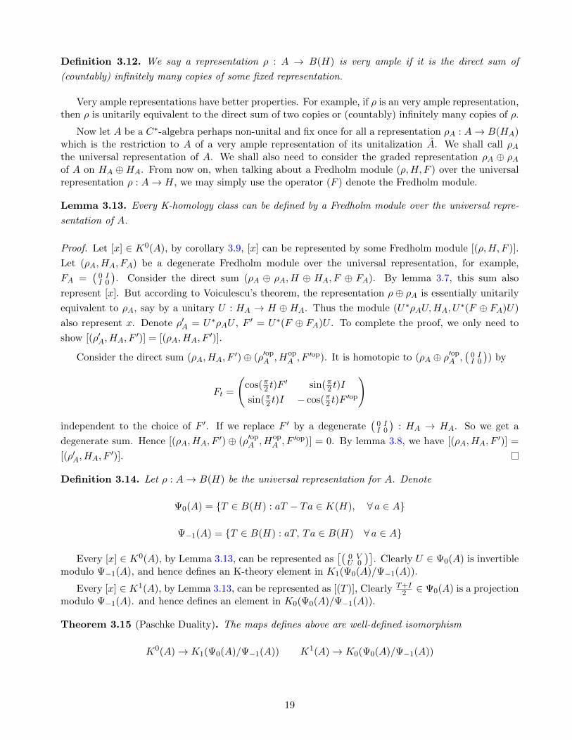
Definition 3.12. We say a representation ρ : A → B(H) is very ample if it is the direct sum of

(countably) infinitely many copies of some fixed representation.

Very ample representations have better properties. For example, if ρ is an very ample representation,then ρ is unitarily equivalent to the direct sum of two copies or (countably) infinitely many copies of ρ.

Now let A be a C∗-algebra perhaps non-unital and fix once for all a representation ρA : A→ B(HA)which is the restriction to A of a very ample representation of its unitalization A. We shall call ρAthe universal representation of A. We shall also need to consider the graded representation ρA ⊕ ρAof A on HA ⊕HA. From now on, when talking about a Fredholm module (ρ,H, F ) over the universalrepresentation ρ : A→ H, we may simply use the operator (F ) denote the Fredholm module.

Lemma 3.13. Every K-homology class can be defined by a Fredholm module over the universal repre-

sentation of A.

Proof. Let [x] ∈ K0(A), by corollary 3.9, [x] can be represented by some Fredholm module [(ρ,H, F )].

Let (ρA, HA, FA) be a degenerate Fredholm module over the universal representation, for example,

FA =(

0 II 0

). Consider the direct sum (ρA ⊕ ρA, H ⊕ HA, F ⊕ FA). By lemma 3.7, this sum also

represent [x]. But according to Voiculescu’s theorem, the representation ρ⊕ ρA is essentially unitarily

equivalent to ρA, say by a unitary U : HA → H ⊕HA. Thus the module (U∗ρAU,HA, U∗(F ⊕ FA)U)

also represent x. Denote ρ′A = U∗ρAU , F ′ = U∗(F ⊕ FA)U . To complete the proof, we only need to

show [(ρ′A, HA, F′)] = [(ρA, HA, F

′)].

Consider the direct sum (ρA, HA, F′)⊕ (ρ′op

A , HopA , F ′op). It is homotopic to (ρA ⊕ ρ′op

A ,(

0 II 0

)) by

Ft =

(cos(π2 t)F

′ sin(π2 t)I

sin(π2 t)I − cos(π2 t)F′op

)

independent to the choice of F ′. If we replace F ′ by a degenerate(

0 II 0

): HA → HA. So we get a

degenerate sum. Hence [(ρA, HA, F′) ⊕ (ρ′op

A , HopA , F ′op)] = 0. By lemma 3.8, we have [(ρA, HA, F

′)] =

[(ρ′A, HA, F′)].

Definition 3.14. Let ρ : A→ B(H) be the universal representation for A. Denote

Ψ0(A) = {T ∈ B(H) : aT − Ta ∈ K(H), ∀ a ∈ A}

Ψ−1(A) = {T ∈ B(H) : aT, Ta ∈ B(H) ∀ a ∈ A}

Every [x] ∈ K0(A), by Lemma 3.13, can be represented as[(

0 VU 0

)]. Clearly U ∈ Ψ0(A) is invertible

modulo Ψ−1(A), and hence defines an K-theory element in K1(Ψ0(A)/Ψ−1(A)).

Every [x] ∈ K1(A), by Lemma 3.13, can be represented as [(T )], Clearly T+I2 ∈ Ψ0(A) is a projection

modulo Ψ−1(A). and hence defines an element in K0(Ψ0(A)/Ψ−1(A)).

Theorem 3.15 (Paschke Duality). The maps defines above are well-defined isomorphism

K0(A)→ K1(Ψ0(A)/Ψ−1(A)) K1(A)→ K0(Ψ0(A)/Ψ−1(A))

19

Section 3.2 Coarse Baum-Connes Conjecture

We shall define an index map from Ki(X) to Ki(C∗(X)). Recall that both groups are defined on the

same fixed separable Hilbert space with the same very ample representation.

Recall that every properly supported pseudo-differential operator can be perturbed by a properlysupported smoothing operator so as to have support confined to a strip near the diagonal X × X.Similarly, we have the following lemma.

Lemma 3.16. D∗(X)/C∗(X) ∼= Ψ0(X)/Ψ−1(X)

Definition 3.17. We define the assembly map µ to be composition of the following maps

Kp(X)∼=−→ Kp+1(Ψ0(X)/Ψ1(X))

∼=−→ Kp+1(D∗(X)/C∗(X))∂−→ Kp(C

∗(M))

where ∂ is the K-theory boundary map.

We cannot expect the assembly map to be always isomorphism, since the right hand side dependson the large scale property of X, while the left hand side depends on the topological property. Thus itis natural to restrict our attention to spaces have no “local topology”.

Definition 3.18. We say a complete Riemannian manifold M is uniformly contractible, if for every

r > 0, there exists R > 0, such that B(x, r) is contractible in B(x,R) for every x ∈M .

It follows from the definition that πn(M) is trivial for all n ≥ 1. Since every complete Riemannianmanifold has homotopy type of CW-complex, by Whitehead theorem, M is contractible.

Conjecture 3.19 (Coarse Baum-Connes Conjecture). The assembly map for uniformly contractible

manifold is an isomorphism.

We can formulate the coarse Baum-Connes conjecture for more general spaces, but we need a processto “kill” all the “local topology”.

Definition 3.20. Let X be a locally finite discrete metric space. For each d > 0, we define the Rips

complex Pd(X) to be the simplicial polyhedron endowed with simplicial metric whose set of vertices equals

to X and where a finite subset {x0, . . . , xn} spans an n-simplex in Pd(X) if and only if d(xi, xj) ≤ d for

all 0 ≤ i, j ≤ n.

The Rips complex Pd(X) encodes the process of “killing the local topology on scale d”, by squeezingeverything of diameter less than d, into a single simplex. As d grows to infinity, all local topology are“smoothed out”.

Recall that the simplicial metric on a simplicial complex is the unique path length metric thatrestricts to the standard Euclidean metric on each simplex. In some references, the spherical metric hasbeen used. Using the simplicial metric is convenient for computation. If a simplicial complex if finitedimensional, then the simplicial metric and the spherical metric are coarse equivalent. Since we willrestrict our attention to the spaces with bounded geometry, Pd(Γ) is always finite-dimensional. Thedifference between the simplicial and the spherical metric is not important.

Clearly, a Rips complex Pd(Γ) is a locally compact complete metric space. By Hopf-Rinow Theorem,Pd(Γ) is proper and geodesic complete.

20

Definition 3.21. We define the coarse K-homology for a locally discrete metric space to be

KX∗(X) := lim−→d

K∗(Pd(X)).

In general, for a locally compact metric space X, we choose a locally finite net Γ, and define

KX∗(X) := KX∗(Γ),

where a c-net Γ for X is a locally finite discrete subspace that d(x,Γ) ≤ c for some c > 0 and all

x ∈ Xand that d(x, y) ≥ c for all x, y ∈ Γ.

It is easy to verify that the coarse K-homology does not depend on the choice of the net. For aproper metric space X, by Zorn lemma, we can always find a net for X.

Suppose that Γ be an r-dense net in X, and that d ≥ r. We choose a partition unity {ϕγ} subordinateto the locally finite open cover {B(γ, d)}γ ∈ Γ, and define ϕ : X → Pd(X) by

ϕ : x→∑γ

ϕγ(x)γ.

Since for each x there are only finitely many γ such that ϕγ(x) 6= 0, it follows that c(x), in barycentriccoordinates, is a point of Pd(X). Passing to the inductive limit, we get a map

c : K∗(X)→ KX∗(X)

which does not depends on the choice of net and the partition of unity.

Remark 3.22. If X be a uniformly contractible manifold with bounded geometry, then

c : K∗(X)∼=−→ KX∗(X)

is an isomorphism.

Recall that a metric space has bounded geometry, if we can choose a net Γ, such that for every

r, #B(γ, r) < N(r) for some Nr for all γ ∈ Γ. The bounded geometry condition is important here.

Dranishnikov, Ferry and Weinberger have constructed an example of uniformly contractible space X for

which c is not an isomorphism [DFW].

It is clear that if X has bounded geometry, Pd(Γ) is finite-dimensional more each d. However, asd increases, the dimension of Pd(Γ) will keep increasing, and become more complicated. For practicalpurposes, we sometimes need to define coarse K-homology in a more flexible way, by anti-Cech sequence.We will use it in the proof for the coarse Baum-Connes conjecture in the finite asymptotic dimensioncase.

Definition 3.23. Let U be a locally finite and uniformly bounded cover for X. We define the nerve

space NU associated to U to be the simplicial complex endowed with the spherical metric whose set of

vertices equals U and where a finite subset {U0, · · · , Un} ⊂ U spans an n-simplex in NU if and only if⋂ni=0 Ui 6= ∅.

21

Definition 3.24. An anti-Cech sequence for a metric space X is a sequence {Ui} of open covers of X

with the property that Lebesgue(Ui) goes to infinity, and Diam(Ui) ≤ Lebesgue(Ui+1).

We can define a simplicial map fi : NUi → NUi+1 such that U ⊂ V whenever f(U) = V . We remarkthat

lim−→j

K∗(NUj )

does not depend on the choice of simplicial map above, and provides another model for KX∗(X).

Remark 3.25. Let X be a uniformly discrete space, we have that

lim−→j

K∗(NUj )∼= lim−→

d

Pd(X)

If fact, let x0, . . . , xn ∈ X and let Ui = Br(xi). If d(xi, xj) < r then U0, . . . , Un have non-empty

intersection. Thus for any d < r we have a map

Pd(X)→ NUr .

Conversely if U0, . . . , Un have non-empty intersection, then d(xi, xj) < 2r, so for d ≥ 2r we have a map

NUr → Pd(X).

Hence

lim−→d

K∗(Pd(X)) ∼= lim−→r

K∗(NUr).

To compare the metric dX on X and dNU on NU , we have the following easy lemma.

Lemma 3.26. Suppose U is a uniformly bounded cover of X and that the diameter of U is bounded by

D. If U1, U2 ∈ U then there is a universal constant depending only on C such that

dX(U1, U2) ≤ CDdNU (U1, U2).

Proof. If a path of length l lying in the 1-skeleton of NU connects U1, U2 then

l ≤ 2DdNU (U1, U2).

A path of length l contains in the n-skeleton of NU , then we can replace γ by a path γ′ that contains

in the n− 1 skeleton of NU , whose length is no more than C l, where C is a universal constant depends

only on n. The result follows by induction.

For each r, we have an assembly map µ : K∗(NUr) → K∗(C∗(NUr)), passing to the direct limit we

get a maplim−→r

K∗(NUr)→ lim−→r

K∗(C∗(NUr))

For a quasi-geodesic space, we can show that NUr is coarse equivalent to X for r large enough. Hencethe right hand side can be identify with K∗(C

∗(X)).

22

Recall that a metric space is called quasi-geodesic at scale d, if ∃λ ≥ 0, for every x, y ∈ X, thereexists x = x0, x1, · · · , xn = y such that d(xi−1, xi) ≤ d and

∑d(xi−1, xi) ≤ λd(x, y).

In general, we cannot expect NUr is coarse equivalent to X for some r. But we still have the followingresult.

Lemma 3.27. Let X be a proper metric space. We have

lim−→r

K∗(C∗(NUr))→ K∗(C

∗(X))

is an isomorphism. [W, Theorem 2.17]

Now we are ready to state the general coarse Baum-Connes conjecture.

Conjecture 3.28 (Coarse Baum-Connes Conjecture). If X is a proper metric space with bounded

geometry the coarse assembly map

µ : KX∗(X)→ K∗(C∗(X)).

is an isomorphism

The injectivity of the conjecture is not true if we drop the bounded geometry condition [Y98].However, there is also an counterexample for surjectivity (with coefficients) with bounded geometrycondition [HLS].

Aside as a guideline to study the index of elliptic operator on noncompact manifold, the coarseBaum-Connes conjecture has many interesting applications in topology and geometry.

Theorem 3.29 (Descent Principle). Let Γ be a countable group whose classifying space BΓ has the

homotopy type of a CW-complex, then the coarse Baum-Connes conjecture for Γ as a metric space with

a proper length metric implies the strong Novikov conjecture for Γ.

Conjecture 3.30 (Gromov-Lawson). Uniformly contractible complete Riemannian manifold can not

have uniformly positive scalar curvature.

Theorem 3.31. Coarse Baum-Connes conjecture implies Gromov-Lawson conjecture.

Proof. Let [D] be the K-homology class of the Dirac operator on M , we can show that [D] 6= 0 ∈ K∗(M).

If the coarse Baum-Connes conjecture holds, then

index([D]) 6= 0 ∈ K∗(C∗(M)).

But if M has uniformly positive scalar curvature k(p), then by Lichnerowicz formula, ([LM] Page 160)

D2 = ∇∗∇+1

4k

must be invertible. Hence index([D]) = 0.

23

Chapter 4

Localization Algebras

In this chapter we shall introduce the localization algebra and formulate a similar Mayer-Vietoris se-quence to compute its K-theory. We shall define a local index map from K-homology to the K-theoryof localization algebra, and prove that it is an isomorphism. Hence the K-theory of localization algebraprovides another model for K-homology. The coarse Baum-Connes assembly map becomes K-theoryhomomorphism induced by an evaluation map, which is much easier to study.

Section 4.1 Localization Algebras

Definition 4.1. Let X be a proper metric space. HX be a nondegenerate X-module. The localization

algebra C∗L(X,HX) is defined to be the C∗-algebra generated by all bounded and uniformly continuous

functions f from [0,∞) to C∗(X,HX) such that

Propagation(f(t))→ 0 as t→∞.

Definition 4.2. A map g from a proper metric space X to another proper metric space Y is called

Lipschitz if

(1) g is a coarse map;

(2) there exists C > 0 such that d(f(x), f(y)) ≤ Cd(x, y).

Definition 4.3. Suppose that g : X → Y is a Lipschtiz map. A uniformly continuous family of

isometries t → V (t): HX → HY , t ∈ [0,∞) is said to cover g if there exists ct > 0, limt→∞

ct = 0, such

that d(g(x), y) ≤ ct.

Lemma 4.4. Let f be a bounded and uniformly continuous function from [0,∞) to B(HX), if there

exist ct > 0, limt→∞

ct = 0 such that Propagation(f(t)) < ct, then f is a multiplier of C∗L(X,HX).

Proof. The proof is exactly similar to Lemma 2.26.

Lemma 4.5. If HY is very ample, then

(1) any Lipschitz map g : X → Y admits a covering family of isometries Vt.

(2) Conjugation by {V (t)} gives ∗-homomorphisms

Ad(V (t)) : C∗L(X,HX)→ C∗L(Y,HY ).

(3) The corresponding maps on K-theory

Kp(C∗L(X,HX))→ Kp(C

∗L(Y,HY ))

24

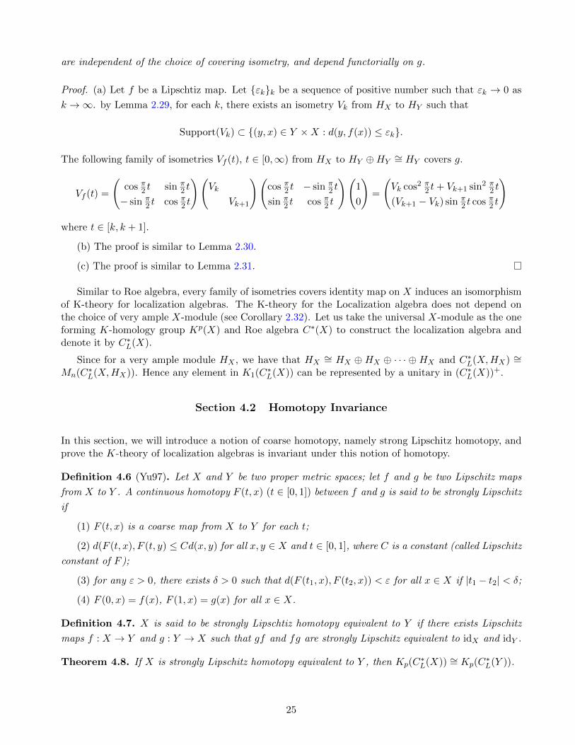
are independent of the choice of covering isometry, and depend functorially on g.

Proof. (a) Let f be a Lipschtiz map. Let {εk}k be a sequence of positive number such that εk → 0 as

k →∞. by Lemma 2.29, for each k, there exists an isometry Vk from HX to HY such that

Support(Vk) ⊂ {(y, x) ∈ Y ×X : d(y, f(x)) ≤ εk}.

The following family of isometries Vf (t), t ∈ [0,∞) from HX to HY ⊕HY∼= HY covers g.

Vf (t) =

(cos π2 t sin π

2 t

− sin π2 t cos π2 t

)(Vk

Vk+1

)(cos π2 t − sin π

2 t

sin π2 t cos π2 t

)(1

0

)=

(Vk cos2 π

2 t+ Vk+1 sin2 π2 t

(Vk+1 − Vk) sin π2 t cos π2 t

)

where t ∈ [k, k + 1].

(b) The proof is similar to Lemma 2.30.

(c) The proof is similar to Lemma 2.31.

Similar to Roe algebra, every family of isometries covers identity map on X induces an isomorphismof K-theory for localization algebras. The K-theory for the Localization algebra does not depend onthe choice of very ample X-module (see Corollary 2.32). Let us take the universal X-module as the oneforming K-homology group Kp(X) and Roe algebra C∗(X) to construct the localization algebra anddenote it by C∗L(X).

Since for a very ample module HX , we have that HX∼= HX ⊕HX ⊕ · · · ⊕HX and C∗L(X,HX) ∼=

Mn(C∗L(X,HX)). Hence any element in K1(C∗L(X)) can be represented by a unitary in (C∗L(X))+.

Section 4.2 Homotopy Invariance

In this section, we will introduce a notion of coarse homotopy, namely strong Lipschitz homotopy, andprove the K-theory of localization algebras is invariant under this notion of homotopy.

Definition 4.6 (Yu97). Let X and Y be two proper metric spaces; let f and g be two Lipschitz maps

from X to Y . A continuous homotopy F (t, x) (t ∈ [0, 1]) between f and g is said to be strongly Lipschitz

if

(1) F (t, x) is a coarse map from X to Y for each t;

(2) d(F (t, x), F (t, y) ≤ Cd(x, y) for all x, y ∈ X and t ∈ [0, 1], where C is a constant (called Lipschitz

constant of F );

(3) for any ε > 0, there exists δ > 0 such that d(F (t1, x), F (t2, x)) < ε for all x ∈ X if |t1 − t2| < δ;

(4) F (0, x) = f(x), F (1, x) = g(x) for all x ∈ X.

Definition 4.7. X is said to be strongly Lipschtiz homotopy equivalent to Y if there exists Lipschitz

maps f : X → Y and g : Y → X such that gf and fg are strongly Lipschitz equivalent to idX and idY .

Theorem 4.8. If X is strongly Lipschitz homotopy equivalent to Y , then Kp(C∗L(X)) ∼= Kp(C

∗L(Y )).

25

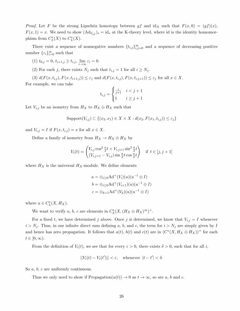
Proof. Let F be the strong Lipschtiz homotopy between gf and idX such that F (x, 0) = (gf)(x),

F (x, 1) = x. We need to show (AdVgf )∗ = id∗ at the K-theory level, where id is the identity homomor-

phism from C∗L(X) to C∗L(X).

There exist a sequence of nonnegative numbers {ti,j}∞i,j=0 and a sequence of decreasing positive

number {εi}∞i=0 such that

(1) t0,j = 0, ti+1,j ≥ ti,j , limi→∞

εi = 0.

(2) For each j, there exists Nj such that ti,j = 1 for all i ≥ Nj .

(3) d(F (x, ti,j), F (x, ti+1,j)) ≤ εj and d(F (x, ti,j), F (x, ti,j+1)) ≤ εj for all x ∈ X.

For example, we can take

ti,j =

ij+1 i < j + 1

1 i ≥ j + 1

Let Vi,j be an isometry from HX to HX ⊕HX such that

Support(Vi,j) ⊂ {(x2, x1) ∈ X ×X : d(x2, F (x1, ti,j)) ≤ εj}

and Vi,j = I if F (x, ti,j) = x for all x ∈ X.

Define a family of isometry from HX → HX ⊕HX by

Vi(t) =

(Vi,j cos2 π

2 t+ Vi,j+1 sin2 π2 t

(Vi,j+1 − Vi,j) sin π2 t cos π2 t

)if t ∈ [j, j + 1]

where HX is the universal HX -module. We define elements

a = ⊕i≥0Ad+(Vi)(u)(u−1 ⊕ I)

b = ⊕i≥0Ad+(Vi+1)(u)(u−1 ⊕ I)

c = ⊕k>1Ad+(Vk)(u)(u−1 ⊕ I)

where u ∈ C∗L(X,HX).

We want to verify a, b, c are elements in C∗L(X, (HX ⊕HX)∞)+.

For a fixed t, we have determined j above. Once j is determined, we know that Vi,j = I whenever

i > Nj . Thus, in our infinite direct sum defining a, b, and c, the term for i > Nj are simply given by I

and hence has zero propagation. It follows that a(t), b(t) and c(t) are in (C∗(X,HX ⊕HX))+ for each

t ∈ [0,∞).

From the definition of Vi(t), we see that for every ε > 0, there exists δ > 0, such that for all i,

||Vi(t)− Vi(t′)|| < ε, whenever |t− t′| < δ.

So a, b, c are uniformly continuous.

Thus we only need to show if Propagation(u(t))→ 0 as t→∞, so are a, b and c.

26

Fix an ε > 0. Let j be such that εj <ε6 , and pick T0 be such that ,

Propogation(u(t)) <ε

2Cfor all t > T0.

Let T1 = max{j, T0}. Then Propagation(f(t0)) ≤ ε for all t0 > T . In fact, to estimate Propogation(f(t0)),

t0 ∈ [j, j + 1], we only need to estimate the propagation of Vi,ju(t0)V ∗i,j , Vi,ju(t0)V ∗i,j+1, Vi,j+1u(t0)V ∗i,j ,

Vi,j+1u(t0)V ∗i,j+1.

Take Vi,j+1u(t0)V ∗i,j as an example. If (x4, x1) ∈ Support(Vi,j+1u(t0)V ∗i,j), then there exists x3, x2

such that (x4, x3) ∈ Support(Vi,j+1), (x3, x2) ∈ Support(u(t0)) and (x2, x1) ∈ SupportV ∗i,j . Hence

d(x4, F (x3, ti,j+1)) ≤ εj , d(x3, x2) ≤ ε6C and d(x1, F (x2, ti,j)) ≤ εj . Since

d(F (x3, ti,j+1), F (x2, ti,j)) ≤ d(F (x3, ti,j+1), F (x3, ti,j)) + d(F (x3, ti,j), F (x2, ti,j))

≤ εj + Cd(x3, x2) ≤ εj +ε

2,

we have that

d(x4, x3) ≤ d(x4, F (x3, ti,j+1)) + d(F (x3, ti,j+1), F (x2, ti,j)) + d(F (x2, ti,j), x1) ≤ εj + εj +ε

2+ εj ≤ ε.

Define

h(s) =∞⊕i=1

Ad+(Vi cos2 π

2s+Vi+1 sin2 π

2s

(Vi+1−Vi) cos π2s sin π

2s

)(u)(u−1 ⊕ I ⊕ I ⊕ I)

By a similar estimation, we can show h(x) ∈ C∗L(X, (HX ⊕HX ⊕HX ⊕HX)∞). This time we need to

estimate Support(Vk,lu(t)Vk′,l′)∗, where k, k′ ∈ {i, i+ 1}, l, l′ ∈ {j, j + 1} and t ∈ [j, j + 1].

If we identify C∗L(X, (HX ⊕HX ⊕HX ⊕HX)∞) and M2(C∗L(X, (HX ⊕HX)∞)), we have

h(0) = a⊕ I, h(1) = b⊕ I

where I is the identity element in C∗L(X, (HX ⊕ HX)∞). Hence a and b represent the same class in

K1(C∗L(X, (HX ⊕HX)∞)).

Since c = Ad+W (b), where W : (HX ⊕HX)∞ → (HX ⊕HX)∞ given by right translation

W : ((v1, v′1), (v2, v

′2), . . .)→ ((0, 0), (v1, v

′1), . . .).

It is clear that W covers the identity map on X, and hence that b and c represent the same class in

K1(C∗L(X, (HX⊕HX)∞)). Thus ac−1 = AdV0(u)(u−1⊕I)⊕I⊕I⊕· · · represent [0] in K1(C∗L(X, (HX⊕HX)∞)). Since the top-left corner inclusion is given by the adjoint of an isometry family, mapping

HX ⊕ HX into the first coordinate in (HX ⊕ HX)∞, which covers covers identity map on X. So it

induces isomorphism K1(C∗L(X,HX⊕HX))→ K1(C∗L(X, (HX⊕HX)∞)). Therefore, AdV0(u) and u⊕Irepresent the same class in K1(C∗L(X,HX ⊕HX)). Since V0 covers gf , so (AdVgf )∗ = id∗.

Section 4.3 Mayer-Vietoris Sequence for K-theory of Localization Algebras

27

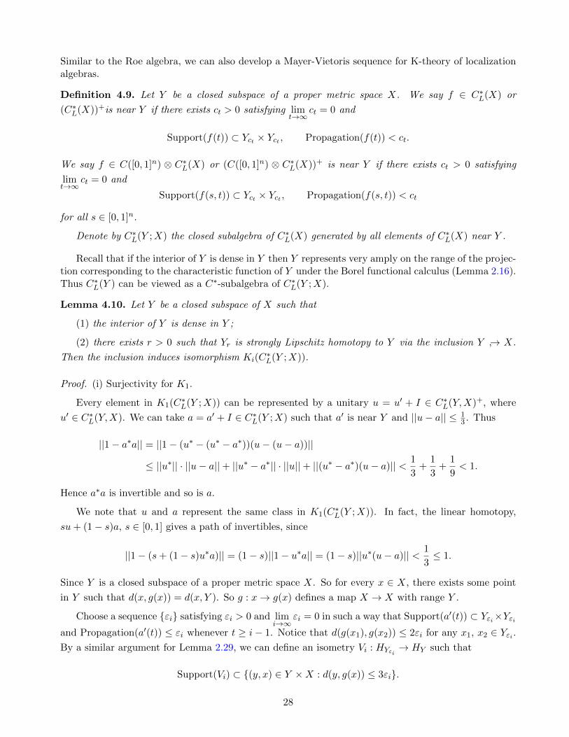
Similar to the Roe algebra, we can also develop a Mayer-Vietoris sequence for K-theory of localizationalgebras.

Definition 4.9. Let Y be a closed subspace of a proper metric space X. We say f ∈ C∗L(X) or

(C∗L(X))+is near Y if there exists ct > 0 satisfying limt→∞

ct = 0 and

Support(f(t)) ⊂ Yct × Yct , Propagation(f(t)) < ct.

We say f ∈ C([0, 1]n) ⊗ C∗L(X) or (C([0, 1]n) ⊗ C∗L(X))+ is near Y if there exists ct > 0 satisfying

limt→∞

ct = 0 and

Support(f(s, t)) ⊂ Yct × Yct , Propagation(f(s, t)) < ct

for all s ∈ [0, 1]n.

Denote by C∗L(Y ;X) the closed subalgebra of C∗L(X) generated by all elements of C∗L(X) near Y .

Recall that if the interior of Y is dense in Y then Y represents very amply on the range of the projec-tion corresponding to the characteristic function of Y under the Borel functional calculus (Lemma 2.16).Thus C∗L(Y ) can be viewed as a C∗-subalgebra of C∗L(Y ;X).

Lemma 4.10. Let Y be a closed subspace of X such that

(1) the interior of Y is dense in Y ;

(2) there exists r > 0 such that Yr is strongly Lipschitz homotopy to Y via the inclusion Y ↪→ X.

Then the inclusion induces isomorphism Ki(C∗L(Y ;X)).

Proof. (i) Surjectivity for K1.

Every element in K1(C∗L(Y ;X)) can be represented by a unitary u = u′ + I ∈ C∗L(Y,X)+, where

u′ ∈ C∗L(Y,X). We can take a = a′ + I ∈ C∗L(Y ;X) such that a′ is near Y and ||u− a|| ≤ 13 . Thus

||1− a∗a|| = ||1− (u∗ − (u∗ − a∗))(u− (u− a))||

≤ ||u∗|| · ||u− a||+ ||u∗ − a∗|| · ||u||+ ||(u∗ − a∗)(u− a)|| < 1

3+

1

3+

1

9< 1.

Hence a∗a is invertible and so is a.

We note that u and a represent the same class in K1(C∗L(Y ;X)). In fact, the linear homotopy,

su+ (1− s)a, s ∈ [0, 1] gives a path of invertibles, since

||1− (s+ (1− s)u∗a)|| = (1− s)||1− u∗a|| = (1− s)||u∗(u− a)|| < 1

3≤ 1.

Since Y is a closed subspace of a proper metric space X. So for every x ∈ X, there exists some point

in Y such that d(x, g(x)) = d(x, Y ). So g : x→ g(x) defines a map X → X with range Y .

Choose a sequence {εi} satisfying εi > 0 and limi→∞

εi = 0 in such a way that Support(a′(t)) ⊂ Yεi×Yεiand Propagation(a′(t)) ≤ εi whenever t ≥ i− 1. Notice that d(g(x1), g(x2)) ≤ 2εi for any x1, x2 ∈ Yεi .By a similar argument for Lemma 2.29, we can define an isometry Vi : HYεi

→ HY such that

Support(Vi) ⊂ {(y, x) ∈ Y ×X : d(y, g(x)) ≤ 3εi}.

28

Vi can also be viewed as a partial isometry HX → HX . Let

V (t) =

(Vi cos2 π

2 t+ Vi+1 sin2 π2 t

(Vi+1 − Vi) cos π2 t sin π2 t

)

We can easily check that V a′, a′V ∗, V a′V ∗ ∈ C∗L(Y ;X), a′V ∗V = a′, and ||V || ≤ 1. By lemma,

[V a′V ∗ + I] = [a] = [u] in K1(C∗L(Y ;X)). But V a′V ∗ ∈ C∗L(Y,HY ). So i∗ is onto.

(ii) Injectivity for K1.

To make our notation simpler, as the proof of surjectivity, we will take every element in the unitalized

algebra with scalar part I. Let [a(t)] ∈ K1(C∗L(Y,HY )) such that i∗[a(t)] = I ∈ K1(C∗L(Y ;X)). Let

h(s, t) be a homotopy in C∗L(Y ;X)+ such that h(0, t) = a(t) and h(1, t) = I. Thus h(s, t) is a unitary in

(C([0, 1])⊗C∗L(Y ;X))+. We will to approximate it by an invertible element in (C([0, 1])⊗C∗L(Y ;X))+

near Y .

There exists an δ > 0 such that

||h(s′, t)− h(s′′, t)|| < 1

2, whenever |s′ − s′′| < δ.

Take N > 1δ and si = i

N , where i = 1, . . . , N − 1. We can take gsi(t) ∈ (C∗L(Y ;Z))+ for each

i = 1, . . . , N − 1, in such a way that ||gsi(t) − h(si, t)|| < 12 , Support(gsi(t)) ⊂ Yci,t × Yci,t and

Propagation(gsi(t)) for some ci,t > 0 satisfying limt→∞

ci,t → 0 and for all t ∈ [0,∞). Define

h′(s, t) =s− si−1

si − si−1gsi(t) +

si − ssi − si−1

gsi−1(t) if s ∈ [si−1, si]

We compute that

||h′(s, t)− h(si, t)||

≤ s− sisi − si−1

||gsi(t)− h(si, t)||+si − ssi − si−1

(||gsi−1(t)− h(si−1, t)||+ ||h(si−1, t)− h(si, t)||) < 1

Thus h′(s, t) is an invertible in (C([0, 1]) ⊗ C∗L(Y ;Z))+. Let ct = maxi{ci,t}; then ct satisfies that

limt→∞

ct = 0, Support(h′(s, t)) ⊂ Yct × Yct and Propagation(h′(s, t)) ≤ ct for all s ∈ [0, 1]. By uniform

continuity of a(t), we know that a(t + sT0), where s ∈ [0, 1], is norm continuous in s for any T0 > 0.

Hence a(t) is equivalent to a(t+ T0) ∈ K1(C∗L(Y ;X)). We can take T0 large enough, such that

Support(h′(s, t+ T0)) ⊂ Yr × Yr for all s ∈ [0, 1].

Hence [a(t)] = [a(t+ T0)] = 0 in K1(C∗L(Yr, HYr)).

We want to remark that the approximation argument also works for (C([0, 1]n)⊗C∗L(Y ;X))+. The

goal is to approximate a unitary in (C([0, 1])n ⊗ C∗L(Y ;X))+ by an invertible element in (C([0, 1]n) ⊗C∗L(X))+ near Y . We divide [0, 1]n evenly into Nn small cubes and approximate the values at vertices

of small cubes by invertibles in C∗L(X)+ near Y , and extend linearly to get an invertible element in

(C([0, 1]n)⊗ C∗L(X))+ near Y .

29

To prove the isomorphism for K0, we will identify K0(A) by K1(C0((0, 1)) ⊗ A). In the proof for

surjectivity (respectively injectivity), we will deal with unitaries in (C([0, 1])⊗C∗L(Y ;X))+ (respectively,

(C([0, 1]2)⊗ C∗L(Y ;X))+) instead. The same “approximation” and “homotopy” arguments apply.

Definition 4.11. Let X be a proper metric space and Y and Z be closed subspaces with X = Y ∪ Z.

Then the decomposition X = Y ∪ Z is said to be strongly excisive if for any ct > 0 with limt→∞

ct = 0,

there exist dt > 0 with limt→∞

dt = 0 such that

Yct ∩ Zct ⊂ (Y ∩ Z)dt

for all t ∈ [0,∞).

Lemma 4.12. Let X = Y ∪ Z be a decomposition of X. Then

C∗L(Y ;X) + C∗L(Z;X) = C∗L(X).

If X = Y ∪ Z is strongly excisive then

C∗L(Y ;X) ∩ C∗L(Z;X) = C∗L(Y ∩ Z;X).

and we have the Mayer-Vietoris sequence

K1(C∗L(Y ∩ Z)) // K1(C∗L(Y ))⊕K1(C∗L(Z)) // K1(C∗L(X))

��K0(C∗L(X))

OO

K0(C∗L(Y ))⊕K0(C∗L(Z))oo K0(C∗L(Y ∩ Z))oo

Proof. The proof is exactly similar to Lemma 2.40, Lemma 2.42, and Theorem 2.43.

Section 4.4 Local Index Map

We can also define a local index map from the K-homology group Ki(X) to the K-theory groupKi(C

∗L(X)).

For each positive integer n, let {Un,i} be a locally finite open cover for X such that diam(Un,i)i < 1/nfor all i. Let {ϕn,i}i be a continuous partition of unity subordinate to {Un,i}i. Let (HX , F ) be a cyclefor K0(X) such that HX is an ample X-module. Define a family of operators F (t) (t ∈ [0,∞) actingon HX by

F (t) =∑i

((1− (t− n))ϕ1/2n,i Fϕ

1/2n,i + (t− n)ϕ

1/2n+1,iFϕ

1/2n+1,i),

for all t ∈ [n, n + 1], where the infinite sum converges in the strong operator topology. Notice thatPropagation(F (t)) is a multiplier of C∗L(X) and F (t) is a unitary modulo C∗L(X). Hence F (t) gives riseto an element [F (t)] in K0(C∗L(X)).

We define the local index of the cycle (HX , F ) to be [F (t)]. Similarly we can define the local indexmap from K1(X) to K1(C∗L(X)).

30

Theorem 4.13. [Yu97] Let X be a simplicial complex endowed with the spherical metric. If X is

finite-dimensional, then the local index map from Ki(X) to Ki(C∗L(X)) is an isomorphism.

The above result has been verified for all proper metric spaces by an Eilenberg swindle argument inthe work of Y. Qiao and J. Roe [QR].

Definition 4.14 (Yu97). Let X be a proper metric space. C∗L,0(X) is defined to be the C∗-algebra

generated by all bounded and uniformly norm continuous functions f from [0,∞) to C∗(X) such that

Propagation(f(t))→ 0 as t→∞, f(0) = 0.

Remark 4.15. We have the following short exact sequence for any proper metric space X,

0→ C∗L,0(X)→ C∗L(X)→ C∗(X)→ 0.

By Theorem 4.13, we identify K∗(X) with K∗(C∗L(X)); thus, to prove the coarse Baum-Connes conjec-

ture, we only need to show that

lim−→d

K∗(C∗L,0(Pd(X)) = 0.

31

Chapter 5

Controlled Obstructions

The concept of controlled obstructions QPδ,r,s,k, QUδ,r,s,k was introduced in my advisor’s work on coarseBaum-Connes Conjecture for spaces with finite asymptotic dimensions [Y98]. Given a representative ofC∗L,0(X), we can not guarantee that it has finite propagation. But we do need finite propagation to allowcutting and pasting technique to work. Given a K-theory element for C∗L,0(X), we will approximate it bya quasi-projection or a quasi-unitary with finite propagation. Apply functional calculus, we can easilyget back the original K-theory element. In this chapter, we will study these controlled obstructions andgive some more details for the results in [Y98].

Section 5.1 Controlled Projections QPδ,r,s,k(X)

Definition 5.1. Let A be a C∗-algebra and δ be a positive number, an element p in A is called a

δ-quasi-projection if

p∗ = p, and ||p2 − p|| < δ.

LetX be a proper metric space. Let C∗L,0(X)+ be the C∗-algebra obtained from C∗L,0(X) by adjoiningan identity. Let δ > 0, r > 0, s > 0, k and n be positive integers.

Definition 5.2. We denote QPδ,r,s,k(C∗L,0(X)+ ⊗Mn(C)) to be the set of all continuous maps from

[0, 1]k to C∗L,0(X)+ ⊗Mn(C) such that:

(1) f(t) is a δ-quasi-projection for all [0, 1]k;

(2) propagation (f(t)) ≤ r for all t ∈ [0, 1]k;

(3) f is piecewise smooth in ti and∥∥∥ ∂f∂ti (t)∥∥∥ ≤ s for all t ∈ [0, 1]k;

(4) ||f(t)− pm|| < δ for all t ∈ bd([0, 1]k);

(5) π(f(t)) = pm, where π is the canonical homomorphism from C∗L,0(X)+ ⊗Mn(C) to Mn(C).

We remark that t = (t1, . . . , tn) can be viewed as suspension parameters. Instead of requiringf(t) = pm on the boundary of [0, 1]n, we allow a more flexible boundary condition, which will add someconvenience to consider suspension map in section 3. By Lemma 5.6 and 5.7, we can normalize theboundary condition if we need.

Definition 5.3. We denote QPδ,r,s,k(X) to be the direct limit of QPδ,r,s,k(C∗L,0(X)+ ⊗Mn(C)) under

the embedding: p→ p⊕ 0.

Definition 5.4. Let p and q be two elements in QPδ,r,s,k(X). Now p is said to be (δ, r, s)-homotopic to

q if there exists a piecewise smooth homotopy a(t′) (t′ ∈ [0, 1]) in QPδ,r,k(C∗L,0(X)+ ⊗Mn(C)) for some

n such that (1) a(0) = p and a(1) = q

(2) ||a′(t′)|| ≤ s.

32

Lemma 5.5. Let 0 < δ < 1 and p(t), q(t) ∈ QPδ,r,s,k(X) satisfying ||p(t) − q(t)|| < δ, then the linear

homotopy a(t′) = t′p+ (1− t′)q is a (2δ, r, s)-homotopy between f and g.

Proof. Clearly a(t′) is self-adjoint. We calculate that

||a(t′)2 − a(t′)|| = ||(t′2 − t′)(p− q) + t′(p2 − p) + (1− t′)(q2 − q)||

≤ (t′2 − t′)δ2 + t′δ + (1− t′)δ ≤ 1

4δ2 + δ ≤ 2δ.

||∂a∂t′|| = ||p− q|| < δ < 1, ||∂a

∂t|| ≤ t′||∂p

∂t||+ (1− t′)||∂q

∂t|| < s.

Lemma 5.6. Let 0 < δ < 10−k. Any p ∈ QPδ,r,s,k(X) is (10k+1δ, r, 2ks)-homotopic to some quasi-

projection q satisfying q(t) = π(q(t)) = pm for some m and all t ∈ bd([0, 1]k).

Proof. For the case k = 1. Let ε = min{ δs ,12}. Let

p1(t) =

ε−tε pm + t

εp(ε) t ∈ [0, ε]

p(t) t ∈ [ε, 1− ε]t−(1−ε)

ε pm + 1−tε p(1− ε) t ∈ [1− ε, 1].

Clearly the propagation of p1(t) is bounded by r. Since the speed of p(t) is bounded by s, we have that

||p(t1)− p(t2)|| ≤ δ, ∀ |t1 − t2| <δ

s.

Hence

||p(t)− pm|| ≤ ||p(t)− p(0)||+ ||p(0)− pm|| ≤ 2δ, ∀ t ∈ [0, ε]

and

||p1(t)− p(t)|| ≤ ε− tε||pm − p(t)||+

t

ε||p(ε)− p(t)|| ≤ ε− t

ε· 2δ +

t

ε· δ ≤ 2δ.

Hence

||p1(t)2 − p1(t)|| =||(p1(t)− p(t))(p1(t)− p(t) + 2p(t)− 1) + (p(t2)− p(t))||

≤||p1(t)− p(t)||(||p1(t)− p(t)||+ 2||p(t)||+ 1 + ||p(t)2 − p(t)||)

≤2δ(2δ + 2√

1 + δ + 1) < 10δ ∀ t ∈ [0, ε].

For the speed of p1(t), we have that∥∥∥∥ ∂∂tp1(t)

∥∥∥∥ =

∥∥∥∥1

ε(pm − p(ε))

∥∥∥∥ ≤ 2δ

ε≤ 2s ∀ t ∈ [0, ε].

We can do similar estimation for t ∈ [1− ε, 1]. We have that p1(t) is a (10δ, r, 2s)-quasi-projection.

33

For the case k > 1, repeating the above process k-times. We get a (10kδ, r, 2ks)-quasi-projection,

such that

||pk(t)− p(t)|| ≤ ||pk(t)− pk−1(t)||+ · · ·+ ||p1(t)− p(t)|| ≤ 2 · 10k−1δ + · · ·+ 2δ < 3 · 10k−1δ,

and π(pk(t)) = pm for all t ∈ bd[0, 1]k. By Lemma 5.5, the linear homotopy between pk(t) and p(t) is a

(10k+1δ, r, 2ks)-homotopy.

Lemma 5.7. Let 0 < δ < 10−k. If p and q are two elements in QPδ,r,s,k(C∗L,0(X)+⊗Mn(C)) such that

p is (δ, r, s)-homotopic to q, p(t) = π(p(t)) and q(t) = π(q(t)) for all t ∈ bd([0, 1]k), then there exists

a (10k+1δ, r, 2ks)-homotopy a(t′) (t′ ∈ [0, 1]) between p and q, such that (a(t′))(t) = π((a(t′))(t)) for all

t′ ∈ [0, 1] and t ∈ bd([0, 1]k).

Proof. Let b(t′) be a (δ, r, s)-homotopy between p and q, since the speed of b(t′) is bounded by s, we

have a equally spaced partition 0 = t′0 < t′1 < · · · t′ms = 1 such that

||b(t′i+1)− b(t′i)|| < δ, b(t′) ∈ QPδ,r,s,k(C∗L,0(X)+ ⊗Mn(C)),

where ms = [ sδ ] + 1 By the proof Lemma 5.6, we can find a(t′i) ∈ QP5·10kδ,r,2ks,k(C∗L(X)+ ⊗M ′n(C)) for

i = 1, . . . ,ms − 1, such that a(t′i)(t) = π(a(t′i)(t)) for all t ∈ bd[0, 1]k and ||a(t′i) − b(t′i)|| < 3 · 10k−1δ.

Hence

||a(t′i)− a(t′i+1)|| ≤ ||a(t′i)− b(t′i)||+ ||b(t′i+1)− b(t′i+1)||+ ||b(t′i+1)− a(t′i+1)||

< 3 · 10k−1δ + δ + 3 · 10k−1δ < 10kδ.

We define

a(t′) =t′ − t′iti+1 − ti

a(ti+1) +t′i+1 − t′

ti+1 − tia(ti) if t′ ∈ [t′i, t

′i+1].

Clearly, we have that π(a(t′)(t)) = a(t′)(t) for all t′ ∈ [0, 1] and t ∈ bd[0, 1]k. By the proof of Lemma 5.5,

we know that for any t′ ∈ [0, 1], a(t′) is a 10k+1δ-quasi-projection with propagation no more than r.

Note that ∥∥∥∥ ∂∂ta(t′)(t)

∥∥∥∥ ≤ 2ks

and ∥∥∥∥ ∂∂t′a(t′)(t)

∥∥∥∥ ≤ 1

ti+1 − ti(||a(ti+1)− a(ti)||) ≤

δ

ms< δ

([sδ

]+ 1)< s+ 1.

We have that the speed of a(t′) is bounded by 2ks.

By the following three lemmas, we can view QPδ,r,s,k(X) as a controlled version of of K0(C∗L,0(X)⊗C0((0, 1)k)).

Lemma 5.8. Let 0 < δ < 1100 , f be a continuous function R satisfying f(x) = 1 for all x ∈ [1/2, 3/2],

and f(x) = 0 for all x ∈ [−1/5, 1/5]. For any p ∈ QPδ,r,s,k(X) satisfying π(p(t)) = pm for some m and

all t ∈ bd[0, 1]k, f(p) is a projection and defines an element [f(p)] in K0((C∗L,0(X)⊗ C0((0, 1)k))+).

34

Proof. Let 0 < δ < 1100 , p ∈ QPδ,r,s,k(C∗L,0(X)+ ⊗Mn(C)). Every λ in the spectrum of p is real and

satisfies |λ2 − λ| < δ, hence

λ ∈(

1−√

1 + 4δ

2,1−√

1− 4δ

2

)∪(

1 +√

1− 4δ

2,1 +√

1 + 4δ

2

)⊂[−1

5,1

5

]∪[

1

2,3

2

].

So f(p) is a projection in (C∗L,0(X) ⊗ C0([0, 1]k))+ ⊗Mn(C) with f(p)(t) = pm for all t ∈ bd[0, 1]k.

Hence f(p) can be viewed as a projection in ((C∗L,0(X)+ ⊗ C0((0, 1)k))+ ⊗Mn(C)).

Lemma 5.9. Let 0 < δ < 1100 , p and q be element in QPδ,r,s,k(X). If a(t′) is a (δ, r, s)-homotopy between

p and q such that π(a(t′)(t)) = pm for some m and all t ∈ bd[0, 1]k, t′ ∈ [0, 1], then [f(p)] = [f(q)] in

K0(C∗L,0(X)⊗ C0((0, 1)k)).

Proof. Given a (δ, r, s)-homotopy a(t′) between p and q, by the continuity of continuous functional calcu-

lus and Lemma 5.7 we have that f(a(t′)) is a continuous path of projections in (C∗L,0(X)⊗C0((0, 1)k)⊗Mn(C))+ connecting f(p) and f(q). Hence [f(p)] = [f(q)] as K-theory elements.

Lemma 5.10. For every 0 < δ < 1100 , every element in K0(C∗L,0(X) ⊗ C0((0, 1)k)) can be represented

as [f(p1)]− [f(p2)], where p1, p2 ∈ QPδ,r,s,k(X) for some r > 0 and s > 0.

Proof. Note that every element in K0(C∗L,0(X))⊗C0((0, 1)k) can be represented as [q1]− [q2], where [q1]

and [q2] are projections in (C∗L,0(X)⊗C0((0, 1)k))+⊗Mn(C) and π(q1) = π(q2) = pm for some m. By the

approximation argument used in Lemma 4.10, we can find p1 and p2 in QPδ/2,r,s,k(C∗L,0(X)+ ⊗Mn(C))

for some r > 0 and s > 0, such that ||pi − qi|| < δ/2 for i = 1, 2, π(p1(t)) = π(p2(t)) = pm for all

t ∈ bd[0, 1]k. By Lemma 5.5, the linear homotopy ai(t′) between pi and qi are (δ, r, s)-equivalences.

It is clear that π(ai(t′)(t)) = pm for all t ∈ bd[0, 1]k and t′ ∈ [0, 1]. Hence by Lemma 5.9, we have

[f(pi)] = [f(qi)] = [qi] ∈ K0((C∗L(X) ⊗ C0((0, 1)k))+) for i = 1, 2. Therefore, [q1] − [q2] = [f(p1)] −[f(p2)] ∈ K0(C∗L(X)⊗ C0(0, 1)k).

Section 5.2 Controlled Unitaries QUδ,r,s,k(X)

In this section, we will approximate elements of K1(C∗L,0(X)) by quasi-unitaries. Most of the resultsare parallel to those in the last section.

Definition 5.11. Let A be a C∗-algebra and δ be a positive number, an element u in A is called a

δ-quasi-unitary if

||u∗u− I|| < δ, and ||uu∗ − I|| < δ

Definition 5.12. We denote QUδ,r,s,k(C∗L,0(X)+ ⊗Mn(C)) to be the set of all continuous functions

from [0, 1]k to C∗L,0(X)+ ⊗Mn(C) such that

(1) f(t) is a delta-quasi-unitary for all t ∈ [0, 1]k;

(2) propagation(f(t)) ≤ r for all t ∈ [0, 1]k;

(3) f is piecewise smooth in ti and∥∥∥ ∂f∂ti (t)∥∥∥ ≤ s for all t ∈ [0, 1]k;

35

(4) ||f(t)− I|| < δ for all t ∈ bd([0, 1]k);

(5) π(f(t)) = I, where π is the canonical homomorphism from C∗L,0(X)+ ⊗Mn(C) to Mn(C)

Definition 5.13. Let QUδ,r,s,k(X) to be the the direct limit of QUδ,r,s,k(C∗L,0(X)+ ⊗Mn(C)) under the

embedding u→ u⊕ I.

Definition 5.14. Let u and v be two elements in QUδ,r,s,k(X). Now u is said to be (δ, r, s)-homotopic

to v if there exists a piecewise smooth homotopy a(t′) (t′ ∈ [0, 1]) in QUδ,r,s,k(C∗L,0(X)+ ⊗Mn(C)) such

that

(1) a(0) = p and a(1) = q;

(2) ||a′(t′)|| ≤ s.

Lemma 5.15. Let 0 < δ < 1 and u, v ∈ QUδ,r,s,k(C∗L,0(X)+ ⊗Mn(C)) satisfying ||u− v|| < δ, then the

linear homotopy a(t′) = (1− t′)u+ t′v is a (2δ, r, s)-homotopy between u and v.

Proof. We calculate that

||a∗(t′)a(t′)− I|| = ||t′(u∗u− I) + (1− t′)(v∗v − I)− (t′ − t′2)(u− v)∗(u− v)||

≤ t′δ + (1− t′)δ + (t′ − t′2)δ2 ≤ δ +1

4δ2 < 2δ.

||∂a∂t′|| = ||u− v|| < δ < 1, ||∂a

∂t|| ≤ t′||∂u

∂t||+ (1− t′)||∂v

∂t|| < s.

Lemma 5.16. Let 0 < δ < 10−k. Every u ∈ QUδ,r,s,k(X) is (10k+1δ, r, 2ks)-homotopic to some quasi-

unitary v satisfying v(t) = π(v(t)) = I for all t ∈ bd([0, 1]k).

Proof. The proof is exactly the same as Lemma 5.6.

Lemma 5.17. Let 0 < δ < 10−k. If u and v are two elements in QUδ,r,s,k(X) such that u is

(δ, r, s)-homotopic to v, u(t) = π(u(t)) and v(t) = π(v(t)) for all t ∈ bd([0, 1]k), then there exists a

(10k+1δ, r, 2ks)-homotopy a(t′) (t′ ∈ [0, 1]) between u and v, satisfying (a(t′))(t) = π((a(t′))(t)) for all

t′ ∈ [0, 1] and t ∈ bd([0, 1]k).

Proof. The proof is exactly the same as Lemma 5.7.

Lemma 5.18. Every u ∈ QUδ,r,s,k(X) satisfying u(t) = π(u(t)) = I for all t ∈ bd([0, 1]k) defines an

element [u] in K1(C∗L,0(X)⊗ C0((0, 1)k)).

Proof. Since ||I − f∗f || < δ < 1, so f∗f invertible. Hence f is invertible, (f∗f)−1f∗ = f∗(ff∗)−1 is its

inverse. So [f ] represent an element in K1(C∗L,0(X)⊗ C0((0, 1)k)).

Lemma 5.19. Let 0 < δ < 12 , u and v be elements in QUδ,r,s,k(X) satisfying u(t) = π(u(t)) =

I and v(t) = π(v(t)) = I for all t ∈ bd([0, 1]k). If u is (δ, r, s)-homotopic to v, then [u] = [v] in

K1(C∗L,0(X)⊗ C0((0, 1)k));

36

Proof. By Lemma 5.15, the elements on the linear path connecting u and v are all 2δ-unitaries, hence

are all invertible.

Lemma 5.20. Every element in K1(C∗L,0(X) ⊗ C0((0, 1)k)) can be represented as [u], where u ∈QUδ,r,s,k(X) for some r > 0 and s > 0 and u(t) = π(u(t)) = I for all t ∈ bd([0, 1]k).

Proof. Every element in K1(C∗L,0(X)⊗C0((0, 1)k)) can be represented as by a unitary v in (C∗L,0(X)⊗C0((0, 1)k) ⊗Mn(C))+ for some n. By the approximation argument used in Lemma 4.10, we can find

u ∈ QUδ,r,s,k((C∗L,0(X))+⊗Mn(C)) for some r > 0 and s > 10 such that ||u−v|| < δ/2. By Lemma 5.15,

u and v are (δ, r, s)-homotopic. Hence by Lemma 5.20, [u] = [v] ∈ K1(C∗L,0(X)⊗ C0((0, 1)k)).

In K-theory, we have that u ⊕ u∗ is homotopic to I ⊕ I for every unitary u. Similarly we have thefollowing lemma.

Lemma 5.21. Let 0 < δ < 10−2. If u ∈ QUδ,r,s,k(X), then there exists a (3δ, 2r, 8s)-homotopy between

I ⊕ I and u⊕ u∗.

Proof. The linear homotopy between I ⊕ I and uu∗ ⊕ I is a (3δ, 2r, 4s)-homotopy and the rotation

homotopy (u ⊕ I)R(t)(u∗ ⊕ I)R∗(t) connecting uu∗ ⊕ I to u ⊕ u∗ is a (3δ, 2r, 4s)-homotopy. So the

combination of two homotopies is a (3δ, 2r, 8s)-homotopy.

In K-theory, we know that if unitary equivalence and homotopy equivalence are stably equivalentconcept for two unitaries. For the controlled obstructions, we have the following similar results.

Lemma 5.22. Let 0 < δ < 10−2. If p and q are elements in QPδ,r,s,k(C∗L,0(X)+ ⊗ Mn(C)) and

u ∈ QUδ,r,s,k(C∗L,0(X)+ ⊗Mn(C)) is such that ||p − u∗qu|| < δ for some small ε > 0, then p ⊕ 0 is

(20δ, 10r, 100s)-homotopic to q ⊕ 0, where 0 ∈Mn(C).

Proof. Let w(t) denote the homotopy between I ⊕ I and u ⊕ u∗. A very crude estimate yields that

w(t)(q ⊕ 0)w∗(t) is a homotopy between q ⊕ 0 and uqu∗ ⊕ 0, which is a (10δ, 10r, 100s)-homotopy. The

linear homotopy between uqu∗ ⊕ 0 and p⊕ 0 is a (20δ, 10r, 200s)-homotopy. So the combination of two

homotopies is a (20δ, 10r, 400s) -homotopy.

Lemma 5.23. Let 0 < δ < 1/100. If p and q are two (δ, r, s)-homotopic elements in QPδ,r,s,k(C∗L,0(X)+⊗

Mn(C)), then there exists u ∈ QUδ,C1(δ,s)r,C2(s),k(C∗L,0(X)+ ×Mn(C)) such that ||p − u∗qu|| < C3(s)δ,

where C1(δ, s) depends only on δ and s, C2(s) and C3(s) depend only on s.

Proof. The idea is that if two quasi-projections are close, then they are “quasi-unitarily equivalent”.

The homotopy provides us a multitude of quasi-unitaries, we will “normalized” them a little bit and take

the product. The bound for the speed of homotopy helps us to control the number of quasi-unitaries in

the product and it is here that we need the speed to be controlled.

Let a(t′) be a (δ, r, s)-homotopy between p and q. Since the speed of a(t′) is bounded by s, we have

an equally spaced partition

0 = t′0 < t′1 < · · · < t′ms = 1

37

such that

||a(t′i+1)− a(t′i)|| <1

100,

where ms depends only on s. Consider

ui = [(2a(t′i+1)− I)(2(a(t′i)− I)) + I]/2,

we have that

||1− ui|| =||(2a(t′i+1)− I)(a(t′i+1)− a(t′i)) + 2(a(t′i+1)− a2(t′i+1))||

≤(2||a(t′i+1)||+ 1) · ||a(t′i+1)− a(t′i)||+ 2||a(t′i+1)− a2(t′i+1)||

≤(2 · 2 + 1) · 1

100+ 2 · 1

100<

1

10.

It follows that

||1− u∗iui|| = ||1− u∗i ||+ ||u∗i || · ||1− ui|| <1

10+ 2 · 1

10=

3

10.

We also have

||a(t′i+1)ui − uia(t′i)||

=||(a(t′i+1)2a(t′i)− 2a(t′i+1)a(t′i)) + 2a(t′i+1)(a2(t′i)− a(t′i))− a(t′i+1)2 + a(t′i+1) + a(t′i)2 − a(t′i)||

≤2||a(t′i+1)2 − a(t′i+1)|| · ||a(t′i)||+ 2||a(t′i+1)|| · ||a2(t′i)− a(t′i)||+ ||a2(t′i+1)− a(t′i+1)||+ ||a2(t′i)− a(t′i)||

≤4δ + 4δ + δ + δ = 10δ.

Let Pl(x) be the l-th Taylor polynomial for 1√1−x at 0. Choose l0 such that∣∣∣∣∣P 2

l0(x)−(

1√1− x

)2∣∣∣∣∣ < δ

4 · 2ms

for all x ∈ [0, 310 ]. Let

wi = uiPl0(1− u∗iui).

We will show that

u = wms−1 · · ·w0

is the the quasi-unitary we are looking for.

First we want to show the speed of u is at most C2(s). Since the speed of a(ti) is at most s, hence

the speed of ui is at most 10s, so the speed of I − u∗iui is at most 40s. Notice that Pl(x) and P ′l (x)

has nonnegative coefficients, hence the sequence of Pl(x) and P ′l (x) is uniformly bounded by 1√1−x and

38

(1√1−x

)′respectively, and

∥∥∥∥ ∂∂tPl0(I − u∗iui)∥∥∥∥

≤P ′l0(||1− u∗iui||) ·∥∥∥∥ ∂∂t(I − u∗iui)

∥∥∥∥< supx∈[0, 3

10]

(1√

1− x

)′· 40s ≤ 40s.

Hence∥∥ ∂∂twi

∥∥ ≤ 100s. So ∥∥∥∥ ∂∂tu∥∥∥∥ ≤ C2s.

for some C2(s) depends only on s.

Next we want to estimate the propagation of u. It is bounded by C1(δ, s)r, where C1 depends only

on l0 and ms, hence depends only on δ and s.

To show u is a δ-unitary, we note that

||1− w∗iwi|| = ||I − u∗iPl0(I − u∗iui)2ui|| ≤

∥∥∥∥∥∥u∗i( 1√

1− (1− u∗iui)

)2

− P 2l (I − u∗iui)

ui

∥∥∥∥∥∥ ≤ δ

2ms.

Hence

||1− u∗u||

=||I − w∗0 · · ·w∗ms−1wms−1 · · ·w0||

≤||I − w∗0 · · ·w∗ms−2wms−2 · · ·w0||+ ||w∗0 · · ·w∗ms−2|| · ||1− w∗ms−1wms−1|| · ||w0 · · ·wms−2||

≤||1− w∗0 · · ·w∗ms−2wms−2 · · ·w0||+ 2ms−1 · δ

2ms≤ · · · ≤ (1 + · · ·+ 2ms−1) · δ

2ms< δ.

To finish the proof, we need to check ||p− u∗qu|| < C3δ. Note that

||u∗iuia(t′i)− a(t′i)u∗iui||

≤||u∗i || · ||uia(t′i)− a(t′i+1)ui||+ ||u∗i a(t′i+1)− a(t′i)u∗i || · ||ui||

<2 · 10δ + 10δ · 2 = 40δ.

Hence

||a(t′i)(I − u∗iui)n − (I − u∗iui)na(t′i)||

≤||(a(t′i)u∗iui − u∗iuia(t′i))(I − u∗iui)n−1||+ ||(I − u∗iui)(a(t′i)u

∗iui − uiu∗i a(t′i))(I − u∗iui)n−2||

· · ·+ ||(I − u∗iui)n−1(a(t′i)u∗iui − uiu∗i a(t′i))|| < 40δn

(3

10

)n−1

.

39

Therefore

||a(t′i)Pl0(I − u∗iui)− Pl0(I − u∗iui)a(t′i)|| < 40δP ′l0

(3

10

)This together with the definition of wi, implies that

||a(t′i+1)wi − wia(t′i)||

≤||a(t′i+1)ui − uiai(t′i)|| · ||Pl0(I − u∗iui)||+ ||ui|| · ||a(t′i)Pl0(I − u∗iui)− Pl0(I − u∗iui)a(t′i)||

≤10δ · 2 + 2 · 40δP ′l0

(3

10

)< 100δ.

Hence

||w∗i a(t′i+1)wi − a(t′i)|| ≤||w∗i || · ||a(t′i+1)wi − wia(t′i)||+ ||w∗iwi − I|| · ||a(t′i)||

<2 · 100δ +δ

2ms· 2 < 300δ.

So

||p− u∗qu||

=||p− w∗0 · · ·w∗ms−1a(t′ms)wms−1 · · ·w0||

≤||p− w∗0 · · ·w∗ms−2a(t′ms−1

)wms−2 · · ·w0||+ ||w∗0 · · ·w∗ms−2|| · ||w∗s−1a(t′ms)ws−1 − a(t′ms−1

)|| · ||ws−2 · · ·w0||

≤||p− w∗0 · · ·w∗ms−2a(t′ms−1

)wms−2 · · ·w0||+ 2ms−1 · 300δ

≤ · · · ≤ (1 + · · ·+ 2ms−1)300δ < 2ms · 300δ.

We can take C3(s) = 2ms300.

Remark 5.24. Since Pl0(I − u∗iui) is self-adjoint,

‖Pl0(I − u∗iui)2 − I‖ ≤

∥∥∥∥∥∥Pl0(I − u∗iui)2 −

(1√

I − (I − u∗iui)

)2∥∥∥∥∥∥+ ‖I − (u∗iui)

−1‖ ≤ 3δ.

Hence Pl0(I − u∗iui) is (6δ, 2l0r, 100s)-equivalent to I. Hence wi = Pl0(I − u∗iui) is (12δ, 3l0r, 300s)-

equivalent to wi. In general for each δ′ > 0, we choose l0 large enough in such a way that∣∣∣∣∣Pl0(x)2 −(

1√1− x

)2∣∣∣∣∣ < δ′

3,

then ui is (12δ, 3l0r, 300s)-equivalent to a δ′-quasi-unitary wi. The trade for decreasing δ to δ′ is that r

increases to 3l0r and s increases to 300s, where l0 depends only on δ′.

Remark 5.25. As in K-theory, every homotopy of projections is implemented by a homotopy of uni-

taries starting from I. We can strengthen the above lemma a little bit. Let a(t′) be the (δ, r, s)-homotopy

between p and q, then there exists a homotopy w(t′) in QUδ2,C1(δ3,s)r3,C2(s),k(X) such that w(0) = I,

40

||p− u∗(t′)a(t′)u(t′)|| < C3(s)δ3. Let

ui(t′) =

I t′ ∈ [0, ti](2a(t′)−I)(a(t′i)−I)+I

2 t′ ∈ [t′i, t′i+1]

ui t′ ∈ [t′i+1, 1]

We similarly have that

‖1− u∗i (t′)ui(t′)‖ <3

10,

∥∥∥∥ ∂∂tu∥∥∥∥ ≤ 2s,

∥∥∥∥ ∂∂t′u∥∥∥∥ ≤ 2s, ∀ t′ ∈ [0, 1]

and that

‖a(t′)ui − uia(t′i)‖ ≤ 10δ ∀ t ∈ [t′i, t′i+1]

We define

wi(t′) = ui(t

′)Pl0(1− u∗i (t′)ui(t′)), u(t′) = wms−1(t′) · · ·w0(t′).

We can similarly proof that wi(t′) satisfies the desired property.

Section 5.3 Controlled Suspensions

In this section, we will further study how QP relates to QU . As in K-theory, K0 and K1 are related bythe suspension map. In this section, we will demonstrate a similar result.

Definition 5.26. For any proper metric space X, let GQPδ,r,s,k(X) to be the set of formal difference

p− q, where p, q ∈ QPδ,r,s,k(X) for some n, and π(p) = π(q).

Definition 5.27. Two elements p− q and p′ − q′ in GQPδ,r,s,k(X) are said to be (δ, r, s)-homotopic if

p′ ⊕ q and q′ ⊕ p are (δ, r, s)-homotopic. An element p− q is said to be (δ, r, s)-homotopic to 0 if p− qis (δ, r, s)-homotopic to I ⊕ 0− I ⊕ 0 for some n that I, 0 ∈Mn(C).

We use pn to denote an infinite matrix with the unit in the first n places along the diagonal.

Recall that every element in K0(A) can be represented as [x−pn]− [pn] for some n and x ∈M2n(A).

Lemma 5.28. Let p − q ∈ GQPδ,r,s,k(X). Then any element p − q ∈ GQPδ,r,s,k(X) is (10δ, r, 10s)-

homotopic to an element p′ − pn for some nonnegative integer n and some p′ ∈ QPδ,r,s,k(C∗L,0(X) ⊗

M2n(C)).

Proof. Let p and q are in QPδ,r,s,k(CL,0(X)+ ⊗Mn(C)), I is the identity matrix in Mn(C). Then

||(I − q)2 − (I − q)|| = ||q2 − q|| < δ.

The homotopy a(t) = ((I − q)⊕ 0) +R(t)(q ⊕ 0)R∗(t) connects I ⊕ 0 and (I − q)⊕ q is a (10δ, r, 10s)-

homotopy. We can take a path ut of scalar unitary matrices in M2n(C) such that u0 = I, u1π(p ⊕(I − q))u∗1 = I ⊕ 0. So u1(p⊕ (I − q))u∗1 ⊕ q is (10δ, r, 10s)-homotopic to (p⊕ (I ⊕ 0)). Hence p− q is

(10δ, r, 10s)- homotopic to u1(p⊕ (1− q))u∗1 − (I ⊕ 0).

41

For any u ∈ QUδ,r,s,k(X), let zt(u) be homotopy connecting I ⊕ I to u ⊕ u∗ demonstrated inLemma 5.21. Let

et(u) = zt(u)(I ⊕ 0)z∗t (u)

It is simply to check that et(u) ∈ QP100δ,100r,100s,k+1(X) and π(et(u)) = I ⊕ 0. So we can define mapfrom QUδ,r,s,k(X) to GQP100δ,100r,100s,k+1(X) by

θ(u) = et(u)− (I ⊕ 0)

where t is the (k + 1)th suspension parameter.

The following lemma shows that the suspension map is well-defined in some sense.

Lemma 5.29. For any 0 < δ < 1100 , r > 0, s > 1, there exist 0 < δ1 < δ, 0 < r1 < r and s1 > 0 such

that if two elements u and v in QUδ1,r1,s,k(C∗L,0(X)+ ⊗Mn(C)) are (δ1, r1, s)-homotopic, then θ(u) and

θ(v) are (δ, r, s1)-homotopic, where δ1 depends only on δ, r1 depends only on r, and s1 depend only on

s.

Proof. Let us, for the moment, assume that δ1 and r1 are small enough and have been determined,

we will demonstrate a homotopy and check to see where it lives, and then pick δ1, r1 accordingly, s1 is

easily determined by seeing how the speed grows. We will apply this kind of argument many times in

the proofs of many following facts.

Let w(t) be the homotopy realizing the (δ1, r1, s)-homotopy between u and v. It is easy to check

that the homotopy w(t)∗u between u∗u and v∗u is a (3δ1, 2r1, 4s)-homotopy. By Lemma 5.15, the linear

homotopy between I and u∗u is a (6δ1, 2r1, 4s)-homotopy. So the combination of these two homotopies

is a (6δ1, 2r1, 8s)-homotopy b(t) between I and v∗u, and we denoted it by a(t). We similarly define a

(6δ1, 2r1, 8s)-homotopy between I and v∗u by combining the linear homotopy between I and uu∗ with

the homotopy w(t)u∗. Define

xt = zt(v)(a(t)⊕ b(t))z∗t (v)

where zt is as in the definition of the map θ. Since by Lemma 5.21, we know that z∗t (v) is a (3δ1, 2r1, 8s)-

homotopy. It is straightforward to check that xt is a (21δ1, 6r1, 96s)-homotopy. We also have that

x0 = I ⊕ 0, ||x1 − I ⊕ I|| = ||vv∗uu∗ ⊕ v∗vu∗u − I ⊕ I|| < 3δ. So xt ∈ QU100δ1,100r1,100s,k+1(X). It is

straightforward to check that

||xtet(u)x∗t − et(v)|| < 48δ1.

By Lemma 5.22, we can safely conclude that et(u)⊕02n is (105δ1, 105r1, 105s)-homotopic to et(v)⊕02n.

Hence we can take δ1 = δ105

, r1 = r105

, s1 = 105s.

The following two lemmas will show that the suspension map is injective and surjective respectivelyin the asymptotic sense.

Lemma 5.30. For any 0 < δ < 1100 , r > 0, s > 1, there exist 0 < δ2 < δ, 0 < r2 < r and s2 > 0

for which if u and v are two elements in QUδ2,r2,s,k(C∗L,0(X)+ ⊗Mn(C)) such that θ(u) and θ(v) are

(δ2, r2, s)-homotopic, then u and v are (δ, r, s2)-homotopic, where δ2 depends only on δ and s; r2 depends

only on δ, r and s; and s2 depends only on s.

42

Proof. As we have seen many examples how to deal with quasi-projections and quasi-unitaries. We will

quicken our pace a little bit. We will not determine some universal constants explicitly, but only clearly

state how they depend with δ, r, s and so on.

By Lemma 5.23, there exists x′ ∈ QUδ2,C1(δ2,s)r2,C2(s),k+1(C∗L,0(X)+ ⊗M4n(C)) such that

||x′(et(u)⊕ In ⊕ 0)x′∗ − (et(v)⊕ In ⊕ 0)|| < C3(s)δ2.

Since In ⊕ 0 = et(In) and that et(u) ⊕ et(In) is unitarily equivalent to et(u ⊕ I), we can find x ∈QUδ2,C1(δ2,s)r,C2(s),k+1(C∗L,0(X)+ ⊗Mn(C)) such that

||x(et(u⊕ In))x∗ − et(v ⊕ In)|| < C3(s)δ2.

This easily implies that

||z∗t (v ⊕ In)xtzt(u⊕ In)(I2n ⊕ 0)− (I2n ⊕ 0)z∗t (v ⊕ In)xtzt(u⊕ In)|| < 1000C3(s)δ2.

where x is identified with a piecewise smooth family of elements xt in QUδ2,C1(δ2,s)r2,C2(s),k(C∗L,0(X)+⊗

M4n(C)), t ∈ [0, 1].

If we write z∗t (v⊕ In)xtzt(u⊕ In) =( ct gtht dt

), we have that ||gt|| < 1000C3(s)δ2, ||ht|| < 1000C3(s)δ2.

We can easily check that z∗t (v ⊕ In)xtz∗t (u⊕ In) is a 100δ2-quasi-unitary for every t ∈ [0, 1]. So ||c∗t ct +

h∗tht − I2n|| < 100δ2. Hence

||c∗t ct − I2n|| = ||c∗t ct + h∗tht − I2n||+ ||h∗tht|| < 100δ2 + 106C3(s)2δ2.

Since ||x0 − I4n|| < δ2, ||x1 − I4n|| < δ2. Thus

||z∗1(v ⊕ In)x0z1(u⊕ In)− I4n|| < 10δ2

‖z∗1(v ⊕ In)x1z1(u⊕ In)− z∗1(v ⊕ In)z1(u⊕ In)‖ < 10δ2

If we write the left hand side of above inequalities in 2 by 2 matrices, and compare the left-top elements,

we have that

||c0 − I2n|| < 10δ2 and ||c1 − (v∗ ⊕ In)(u⊕ In)|| < 10δ2.

Combine the linear homotopy between I2n and c0, the homotopy ct, the linear homotopy between c1 and

(v∗⊕In)(u⊕In), we get a (M1(s)δ2,M2(δ2, s)r2,M3(s))-homotopy a(t) between I2n and (v∗⊕In)(u⊕In),

for some constant M1, M2 and M3.

Let b(t) be the linear homotopy connecting vv∗ ⊕ In and I2n. Then the combination of homotopies

(v⊕ I)a(t) and b(t)(u⊕ I) is a (M1(s)δ2, M2(δ2, s)r2, M3(s))- homotopy between (v⊕ In) and (u⊕ In).

For some constant M1, M2 and M3. Now we get the desired result by picking appropriate δ2, r2 and

s2.

Lemma 5.31. For any 0 < δ < 1100 , r > 0, s > 10, there exist 0 < δ3 < δ, 0 < r3 < r and s3 > s, such

that for any p− pn ∈ GQPδ3,r3,s,k(C∗L,0(X)+⊗M2n(C)), there exists u ∈ QUδ,r,s3,k(X) for which θ(u) is

43

(δ, r, s3)-homotopic to p− pm, where δ3 depends only on δ and s, r3 depends only on δ, r and s; and s3

depends only on s.

Proof. We identify p as a piecewise smooth path in QPδ,r,s,k(C∗L,0(X)+ ⊗M2n(C)). By Remark 5.25,

there exists a homotopy w(t) in QUδ3,C1(δ3,s)r3,C2(s),k(C∗L,0(X)+⊗M2n(C)) such that w(0) = I2n, ||p(0)−

w(t)∗p(t)w(t)|| < C3(s)δ3. It follows that

||w(1)p(0)− p(1)w(1)|| < 10C3(s)δ3.

Since ||p(0)− In ⊕ 0|| < δ3, ||p(1)− In ⊕ 0|| < δ3, we have that

||w(1)(In ⊕ 0)− (In ⊕ 0)w(1)|| < 4δ3 + 10C3(s)δ3.

So we can write w(1) = ( u gh v ), where ||g|| < 4δ3 + 10C3(s)δ3, ||h|| < 4δ3 + 10C3(s)δ3. Hence u and v are

(1 + (4δ3 + 10C3(s))2)δ3-quasi-unitaries. Let

yt = (w(t)⊕ In)(In ⊕ z∗t (v)w∗(t))(z∗t (u)⊕ In).

It is straightforward to check that y0 = I and there exists a universal constant C3(s) depend only on s

such that yt is a C3(s)-quasi-unitary and that

||y1 − I|| < C3(s)δ3, ||yt(zt(u)⊕ In)(In ⊕ 0)(zt(u)∗ ⊕ In)y∗t − (p⊕ 0)|| < C3(s)δ3.

Then apply Lemma 5.22, we have that et(u)⊕ 0 and p⊕ 0 are homotopic, hence et(u)⊕ pn and p⊕ pnare homotopic. Again, by picking appropriate r3, and s3, we get the desired result.

Section 5.4 Invariance under Strong Lipschtiz Homotopy

We have seen in Theorem 4.8 that the K-theory of localization algebra is invariant under strong Lipschitzhomotopy. For the controlled obstructions, we have the following similar result.

Lemma 5.32. Let f and g be two proper Lipschitz maps from X to Y . Assume that f is strongly

Lipschtiz homotopic to g. There exists S0 > 0, C0 > 0 such that for any u ∈ QUδ,r,s,k(X), there exists a

(C0δ, C0r, C0s)-homotopy between w(0) = Ad(Vf )(u)⊕ I, and w(1) = Ad(Vg)(u)⊕ I, where C0 depends

only on the Lipschitz constant C of the strong Lipschitz homotopy between f and g.

Proof. Let F be the strong Lipschitz homotopy between f and g such that F (x, 0) = f(x), F (x, 1) =

g(x).

There exist a sequence of nonnegative numbers {ti,j | 0 ≤ i ≤ ∞, 0 ≤ j < ∞} and a sequence of

decreasing positive number {εi}∞i=0 such that

(1) t0,j = 0, ti+1,j ≥ ti,j , ti,j+1 ≤ tij .

(2) For each j, there exists Nj such that ti,j = 1 for all i ≥ Nj .

(3) d(F (x, ti,j), F (x, ti+1,j)) ≤ εj = rj+1 and d(F (x, ti,j), F (x, ti,j+1)) ≤ εj for all x ∈ X.

44

Let Vi,j be an isometry from HX to HX ⊕HX such that

Support(Vi,j) ⊂ {(x2, x1) ∈ X ×X : d(x2, F (x1, ti,j)) ≤ εj}

Define a family of isometry HX → HX ⊕HX by

Vi(t) =

(Vi,j cos2 π

2 t+ Vi,j+1 sin2 π2 t

(Vi,j+1 − Vi,j) sin π2 t cos π2 t

)if t ∈ [j, j + 1]

where HX is the universal HX -module. Consider

ui(t) = Vi(t)u(t)V ∗i (t) + (I − Vi(t)V ∗i (t)),

where I is the identity map on HX ⊕HX . So u = Ad+(Vf )(u), u∞ = Ad+(Vg)(u). For each i, define

ni to be the largest integer j satisfying i ≥ Nj if {j : i ≥ Nj} 6= ∅, and define ni to be 0 otherwise. We

can choose Vi,j such that ui(t) = u∞(t) when t ≤ ni by taking Vi,j = V∞,j , whenever ti,j = 1. Define

wi(t) =

ui(t)(u∞(t))∗ if t ≥ ni(ni − t)I + (t− ni + 1)ui(t)(u∞(t))∗ if ni − 1 ≤ t ≤ niI if 0 ≤ t ≤ ni − 1.

Consider

a = ⊕∞i=0(wi ⊕ I)

b = ⊕∞i=0(wi+1 ⊕ I)

c = (I ⊕ I)⊕∞i=1 (wi ⊕ I)

where I is the identity operator on HX ⊕HX . Similar to the proof of Theorem 4.8, we can verify that

a, b, c are elements in C∗L(X, (HX ⊕ HX ⊕ HX ⊕ HX)∞)+, and it is easily to check that a, b, c are

elements in QUC1δ,C1r,C1s,k(Y ) for some constant C1 depending only on the Lipschitz constant C.

We will construct a homotopy between a and b by constructing a homotopy wi,i+1(t′) between

wi(t) ⊕ I and wi+1(t) ⊕ I for each i. The idea is simple enough, we will replace Vi(t) in wi(t) ⊕ I by

Vi+1(t) through a “rotation” homotopy, then joining with wi+1(t) linearly. To be more precise we define

that

ui,i+1(t′) =

(Vi cos2 πt′ + Vi+1 sin2 πt′

(Vi − Vi+1) cosπt′ sinπt′

)u

(Vi cos2 πt′ + Vi+1 sin2 πt′

(Vi − Vi+1) cosπt′ sinπt′

)∗

wi,i+1(t′) =

I ⊕ I if 0 ≤ t ≤ ni − 1

(ni − t)(I ⊕ I)− (t− ni + 1)ui,i+1(t)(t′)(u∞(t)⊕ I)∗ if ni−1 ≤ t ≤ niui,i+1(t)(t′)(u∗∞(t)⊕ I) if t ≥ ni

wi,i+1(t′) = (2t′ − 1)(wi+1 ⊕ I) + (2− 2t′)wi,i+1

(1

2

)if 0 ≤ t′ ≤ 1

2

45

h1(t′) = ⊕∞i=0wi,i+1(t′) if 0 ≤ t′ ≤ 1.

Similar to the proof of Theorem 4.8, we can check that for each t′ ∈ [0, 12 ], h1(t′) ∈ CL,0(X, (HX ⊕HX ⊕

HX ⊕HX)∞). It is easily to check that h1(t) is a (C2δ, C2r, C2s)-homotopy for some C2 > C1, where

C2 depends only on C.

Next we will construct a homotopy between b and c, where I is the identity map on HX ⊕HX . Let

V be the isometry on (HX ⊕HX)∞ by right translation, then V bV ∗ = c, consider the homotopy

h2(t′) = R(t′)

(I

V

)R(t′)∗

(b

I

)R(t′)

(I

V ∗

)R(t′)∗

where I is the identity operator on (HX ⊕HX)∞. It is easily to check that h2(t′) is a (C3δ, C3r, C3s)-

homotopy for some constant C depends only on C.

Finally, we define w(t′) to be the homotopy obtained by combining the following homotopies:

(1) The linear homotopy between

(u0 ⊕ I)⊕∞i=1 (I ⊕ I) and c∗a((u∞ ⊕ I)⊕∞i=1 (I ⊕ I)).

(2) h∗2(1− t′)a((u∞ ⊕ I)⊕∞i=1 (I ⊕ I)).

(3) h∗1(1− t′)a((u∞ ⊕ I)⊕∞i=1 (I ⊕ I)).

(4) The linear homotopy between

a∗a((u∞ ⊕ I)⊕∞i=1 (I ⊕ I)) and (u∞ ⊕ I)⊕∞i=1 (I ⊕ I).

Section 5.5 Controlled Cutting and Pasting

In this section, we will study the cutting and pasting techniques for controlled obstructions.

Definition 5.33. Let X be a proper metric space and let Xi for i = 1, 2 be metric subspaces. The triple

(X;X1, X2) is said to satisfy excision condition if

1. X = X1 ∪X2 where Xi is closed subset of X with interior of Xi dense in Xi.

2. For any r > 0, bdr(X1) ∩ bdr(X2) = bdr(X1 ∩X2).

We remark that if X is geodesic complete proper metric space. In particular, X is a locally compactsimplicial polyhedron, we have that for any decomposition X = X1 ∪ X2, where Xi is closed, thecondition 2 in the above definition always holds.

Given (X;X1, X2) satisfying the excision condition, we might want to construct a boundary map∂ : QUδ,r,s,k(X)→ GQPδ′,r′,s′,k(X1 ∩X2). However, in order to account for the propagation, we would“fatten” X1 ∩X2 a little bit. To be more precise, for u ∈ QUδ,r,s,k(X) define uX1 = χX1uχX1 + χX−X1 .Then let

w =

(I uX1

0 I

)(I 0−u∗X1

I

)(I uX1

0 I

)(0 −II 0

)46

and again note that

w =

(uX1 0

0 u∗X1

)+

(uX1(I − u∗X1

uX1) uX1u∗X1− I

I − u∗X1uX1 0

)A very rough estimate yields ||w|| ≤ 10. Hence ||w∗w|| ≤ 100. So w∗1w1 ≤ 100. Note that w is invertible,hence w∗w is positive and invertible. For

w−1 =

(0 I−I 0

)(I −uX1

0 I

)(I 0u∗X1

I

)(I −uX1

0 I

)We similarly have ||w−1|| ≤ 10, ||w∗−1w−1|| ≤ 100, w∗−1w−1 ≤ 100. So w∗w ≥ 1

100 . Hence

0 ≤ I − w∗w

100≤ 1− 1

1002.

This observation allow us to convert w into a δ-quasi-unitary. In fact, let Pl(x) be the l-th Taylorpolynomial for 1

10√

1−x . Choose l(δ) to be the smallest integer such that∣∣∣∣Pl(x)− 1

10√

1− x

∣∣∣∣ < δ

104, ∀x ∈

[0, 1− 1

1002

],

which easily implies that∣∣∣∣∣Pl(x)2 −(

1

10√

1− x

)2∣∣∣∣∣ < δ

100, ∀x ∈

[0, 1− 1

1002

].

Let wu = wPl(I − w∗w100 ), then

‖I − w∗uwu‖ =

∥∥∥∥∥I − w∗Pl(I − w∗w

100

)2

w

∥∥∥∥∥=

∥∥∥∥∥∥w∗ 1

10√I − (I − w∗w

100 )

2

− P 2l

(I − w∗w

100

)w

∥∥∥∥∥∥ ≤ δHence wu is a δ-quasi-unitary. To estimate the propagation of wu, we notice that the largest power ofx in Pl(x) is l, so the propagation of Pl(I − w∗w

100 ) is at most 2lr, and hence that the propagation of wuis at most 3lr. Thus wu(I ⊕ 0)w∗u will have propagation no larger than 10lr. We will enlarge the regionX1 ∩X2 for the propagation of wu(I ⊕ 0)w∗u. For a closed subset A of X, such that the interior of A isdense in A and bd10lr(X1 ∩X2) ⊂ A. We define ∂0(u) = χAwu(I ⊕ 0)w∗uχA.

Lemma 5.34. ∂0(u) ∈ QPN0δ,N(δ)r,N0s,k(A) for some universal constat N0 ≥ 1.

47

Proof. We first verify that ∂0(u) is quasi-projection on HA. In fact,

||∂0(u)2 − ∂0(u)||

=||χA((wu(I ⊕ 0)w∗u)2 − wu(I ⊕ 0)w∗u)χA − χAwu(I ⊕ 0)w∗uχX−Awu(I ⊕ 0)w∗uχA||

≤||(wu(I ⊕ 0)w∗u)2 − wu(I ⊕ 0)w∗u||+ ||χAwu(I ⊕ 0)w∗uχX−Awu(I ⊕ 0)w∗uχA||

≤||wu(I ⊕ 0)(w∗uwu − I)(I ⊕ 0)w∗u||+ 2||χAwu(I ⊕ 0)w∗uχX−A||

<2δ + 2||χAwu(I ⊕ 0)w∗uχX1−A||+ 2||χAwu(I ⊕ 0)w∗uχX2−A||.

To estimate ||χAwu(I ⊕ 0)w∗uχX2−A||, we note that (X2 − A) ∩ X1 = ∅. Thus χX2−A commute with

uX1 hence u and wu. Therefore

||χAwu(I ⊕ 0)w∗uχX2−A|| = 0

To estimate ||χAwu(I ⊕ 0)w∗uχX1−A||. The key observation is that by the excision condition, the

distance between X1−A and X2 is at least 10lr, recall that the propagation of wu(I⊕ 0)w∗u is less than

10lr, so X1 − A is far away enough from X2, hence wu(I ⊕ 0)w∗u cannot move it out of X1. So we can

replace uX1 by u in the construction of wu if we just consider the restriction on X1 − A. In this case,

we can calculate that

w(I ⊕ 0)w∗ =

(uu∗ + 2u(I − u∗u)u∗ + u(I − u∗u)2u∗ u(I − u∗u) + u(I − u∗u)2

(I − u∗u)u∗ + (I − u∗u)2u∗ (1− u∗u)2

)

and thus that ||w(I ⊕ 0)w∗ − (I ⊕ 0)|| < 10δ. Notice that P ′l (x) has nonnegative coefficient, hence

{P ′l (x)}l is uniformly bounded, we can apply a similar estimation used in the proof of Lemma 5.23, to

conclude that there exists a universal constant N ′ such that

||(wu(I ⊕ 0)w∗u − (I ⊕ 0))χX1−A|| < N ′δ

Therefore, ∂0(u) is a N1δ-quasi-projection, where N1 is a universal constant.

We have already seen that the propagation of ∂0(u) is at most 10lr. Since l depends on δ, so we can

take N(δ) as 10l.

To estimate the speed of ∂(u), we can apply a similar argument used in the proof of Lemma 5.23,

to conclude that it is bounded by N2s for some universal constant N2. Now we may take N0 =

max{N1, N2}.

Remark 5.35. Similar to the estimation of ||χAwu(I ⊕ 0)w∗uχX1−A||, we can show that

||(wu − w)χX1−A|| < Nδ,

||χX1−A(wu − w)|| < Nδ

for some universal constant N . In fact,∥∥∥∥∥(w −

(u

u∗

))χX1−A

∥∥∥∥∥ =

∥∥∥∥∥(u(1− u∗u) uu∗ − 1

1− u∗u 0

)∥∥∥∥∥ < 4δ.

48

Hence

||(I − w∗w)χX1−A|| < 20δ.

Thus ∥∥∥∥(I − w∗w

100

)χX1−A

∥∥∥∥ =

∥∥∥∥( 99

100I +

(I − w∗w

100

))χX1−A

∥∥∥∥ < 992

1000

Since Pl(x) has nonnegative coefficients, hence uniformly bounded. Applying a similar estimation used

in the proof of Lemma 5.23, we can show that∥∥∥∥[Pl (I − w∗w

100

)− Pl

(I − I

100

)]χX1−A

∥∥∥∥ < N ′δ

for some universal constant. Hence∥∥∥∥(Pl (I − w∗w

100

)− I)χX1−A

∥∥∥∥=

∥∥∥∥[Pl (I − w∗w

100

)− Pl

(I − I

100

)]χX1−A

∥∥∥∥+

∥∥∥∥(Pl (I − I

100

)− I)χX1−A

∥∥∥∥<N ′δ +

1

104δ

So

||(wu − w)χX1−A|| =∥∥∥∥(wPl (I − w∗w

100

)− w

)χX1−A

∥∥∥∥ < 2

(N ′δ +

1

104

)δ.

Hence

||(wu − (u⊕ u∗))χX1−A|| ≤ ||(wu − w)χX1−A||+ ||(w − (u⊕ u∗))χX1−A|| < 2

(N ′ +

1

104

)δ + 4δ = Nδ,

where N = 2(N ′ + 1104

) + 4 is a universal constant.

Similarly, we have that

||(w∗u − (u∗ ⊕ u))χX1−A|| < Nδ.

Hence

||χX1−A(wu − (u⊕ u∗))|| < Nδ.

Definition 5.36. We define the boundary of u by ∂(u) = ∂0(u)− (I ⊕ 0).

Definition 5.37. We define j : QUδ,r,s,k(X1)⊕QUδ,r,s,k(X2)→ QUδ,r,s,k(X) by

j(u1 ⊕ u2) = (u1 + χX2−A)⊕ (u2 + χX1−A).

Lemma 5.38. Let (X;X1, X2) be as in Definition 5.33. For any 0 < δ < 1100 , r > 0, s > 10, there

exists 0 < δ1 < δ, 0 < r1 < r, s1 > s such that ∂j(u1 ⊕ u2) is (δ, r, s1)-homotopic to 0 for any

ui ∈ QUδ1,r1,s,k(Xi) (i = 1, 2) where δ1 depends only on δ, r1 depends only on r and δ, s1 depends only

on s.

Proof. We will consider each part of the direct sum separately. For u1 ∈ QUδ1,r1,s,k(X1), (j1(u1))X1=

j1(u1) which is a δ1-quasi-unitary. By the same estimate as for ||χAwu(I⊕0)w∗uχX2−A|| in Lemma 5.34,

49

we have that ||∂0j1(u1) − (I ⊕ 0)|| < N ′δ1 for some universal constant N ′. Hence if we take δ1 ≤ δ2N1

,

r1 ≤ rN(δ1) , s1 ≥ N1s, where N1 as Lemma 5.34 Then by Lemma 5.5, the linear homotopy between

∂0(j1(u)) and I ⊕ 0 is a (δ, r, s1)-homotopy.

In the definition of ∂0(u), we first “chop” u by χX1 to get uX1 = χX1uχX1+χX−X1 . Now we will chop

u by χX−X2 , and define uX−X2 = χX−X2uχX−X2 +χX2 . Using uX−X2 , we do the same construction, we

will get w′ and w′u. Let a(t) be the linear homotopy connecting wu and w′u. Applying the same argument

in Lemma 5.34, we have that for any t ∈ [0, 1], χAa(t) ⊕ (I ⊕ 0)a∗(t)χA ∈ QP2N0δ1,N(δ)r1,N0s,k(A). In

fact, we only need to note that χX2−A commute with w′u and a(t)(I ⊕ 0)a∗(t) can not move X1−A out

of X − X2. Hence χAa(t)(I ⊕ 0)a∗(t)χA is a (2N0δ1, N(δ)r1, N0s)-homotopy. Since (j2(u))X−X2 = I,

hence w′ = I, w′u = Pl(99100) which is (δ1, 0, 1)-homotopic to (I ⊕ 0). Hence if we choose δ1 ≤ δ

2N0,

r1 ≤ rN(δ) , s1 ≥ 2N0s, we have that ∂0(j2(u)) is (δ, r, s1)-homotopic to (I ⊕ 0).

Lemma 5.39. Let (X;X1, X2) be as Definition 5.33. For any 0 < δ < 1100 , r > 0, s > 10, there

exists 0 < δ2 < δ, 0 < r2 < r, s2 > s such that if u is an element in QUδ2,r2,s,k(X) for which ∂(u) is

(δ2, r2, s)-homotopic to 0 in GQPδ2,r2,s,k(X1 ∩X2) then there exists ui ∈ QUδ,r,s2,k(Xi) (i = 1, 2) such

that j(u1⊕ u2) is (δ, r, s2)-homotopic to u. Where δ2 depends only on δ and s; r2 depends only on δ, r,

s; and s2 depends only on s.

Proof. Since ∂(u) is (δ2, r2, s)-homotopic to 0, and hence by definition, we have that χAwu⊕I(I ⊕0)w∗u⊕IχA is (δ2, r2, s)-homotopic to I ⊕ 0. By Proposition 5.22, we have that there exists a y ∈QUδ2,C1(δ2,s),C2(s),k(A) such that

||yχAwu⊕I(I ⊕ 0)w∗u⊕IχAy∗ − (χA ⊕ 0)|| < C3(s)δ2 (5.1)

Let x = y+χX1−A. Then x is a δ2-quasi-unitary on X1∪A. Since χX1∪A commute with w, hence wu⊕I ,

we compute that

||xwu⊕I(χX1∪A ⊕ 0)w∗u⊕Ix∗ − (χX1∪A ⊕ 0)||

=||xwu⊕I(I ⊕ 0)w∗u⊕Ix∗ − (χX1∪A ⊕ 0)||

=||yχAwu⊕I(I ⊕ 0)w∗u⊕IχAy∗ − (χA ⊕ 0)||+ ||χX1−Awu⊕I(I ⊕ 0)w∗u⊕IχAy

∗||

+ ||yχAwu⊕I(I ⊕ 0)w∗u⊕IχX1−A||+ ||χX1−Awu⊕I(I ⊕ 0)w∗u⊕IχX1−A − (χX1−A ⊕ 0)||.

Since in the proof Lemma 5.34, we have already demonstrated that

||(wu(I ⊕ 0)w∗u − I ⊕ 0)χX1−A|| < N ′δ2.

Hence the sum of last three terms is no more than 10N ′δ2. This together with (5.1) implies that

||xwu⊕I(χX1∪A ⊕ 0)w∗u⊕Ix∗ − (χX1∪A ⊕ 0)|| < (10N ′ + C3(s))δ2.

This easily implies that

||xwu⊕I(χX1∪A ⊕ 0)− (χX1∪A ⊕ 0)xwu⊕IχX1∪A|| < 10(10N ′ + C3(s))δ2

50

which in turn implies that xwu⊕IχX1∪A is a matrix of the form(v1 bc d

)with

||b|| ≤ 10(10N ′ + C3(s2))δ2, ||c|| ≤ 10(10N ′ + C3(s2))δ2.

This allows us to conclude that v1 is a (M1(s)δ2,M2(δ2, s)r2,M3s)-quasi-unitary on HX1∪A. By Re-

mark 5.35, we have that

‖χX1−A(wu⊕I − (u⊕ I)⊕ (u∗ ⊕ I))‖ < Nδ2

for some universal constant N . Since χX1−Axwu⊕IχX1∪A = χX1−Awu⊕IχX1∪A = χX1−Awu⊕I , and since

v1 is the left-top element in xwu⊕I , we have that

‖χX1−A(v1 − u⊕ I)‖ < Nδ2

Hence

||χX1−A((u⊕ I)v∗1 − I)|| ≤ ||χX1−A((u⊕ I)− v1)v∗1||+ ||χX1−Av1v∗1 − χX1−A||

< (2N +M1(s))δ2

and

||((u⊕ I)v∗1 − I)χX1−A|| ≤ ||(u⊕ I)(v∗1 − (u⊕ I)∗)χX1−A||+ ||((u⊕ I)(u⊕ I)∗ − I)χX1−A||

≤ (2N +M1(s))δ2.

We now need a quasi-unitary that lives on X2 ∪ A. The basic idea is that we want to “divide out”

what’s left of u⊕ I, as we already know that v1 is the “quasi”-adjoint of u⊕ I on X1 −A.

We now define v2 as follow

v2 = χA∪X2(u⊕ I)v∗1χA∪X2

where v1 = v1 + χX2−A. We calculate that

||v2v∗2 − χA∪X2 ||

=||χA∪X2(u⊕ I)v∗1 v1(u⊕ I)∗χA∪X2 − χA∪X2 ||+ ||χA∪X2(u⊕ I)v∗1χX1−Av1(u⊕ I)∗χA∪X2 ||

<3M1(s)δ2 + 4(2N +M1(s))δ2

Similarly, we can show that ||v∗2v2−χA∪X2 || has the same bound. Hence v2 is a (M ′1(s)δ2,M′2(δ2, s)r2,M3(s))-

quasi-unitary for some universal constant M ′1(s), M ′2(δ2, s) and M ′3(s).

To finish the proof, we only need to check that (v1 +χX2−A)⊕ (χX1−A⊕v2) is homotopic to 0. Since

‖(χX1−A + v2)(v1 + χX2 −A)⊕ I − (u⊕ I)‖

=||χX1−Av1 + χA∪X2(u⊕ I)v∗1 v1 − χA∪X2(u⊕ I)v∗1χX1−Av1 − (u⊕ I)||

≤||χX1−A(v1 − u⊕ I)||+ ||χA∪X2(u⊕ I)(v∗1 v1 − 1)||+ ||χA∪X2(u⊕ I)v∗1χX1−Av∗1||

≤Nδ2 + 2M1(s1)δ2 + (2N +M1(s))δ2.

51

Hence by combining the rotation homotopy R(t)(I⊕(v2+χX1−A))R(t)∗((v1+χX2−A)⊕I) and the linear

homotopy between (χX1−A + v2)(v1 +χX2−A)⊕ I and (u⊕ I)⊕ I, and picking appropriate δ2, r2, s2, we

get the desired result.

Remark 5.40. If we further require that ∃R0 > 0, C0 > 0 for each X ′ = X1, X2, X1 ∩ X2, and any

r < r0, bd(X ′) is strongly Lipschitz homotopy equivalent to X ′ with c0 as Lipschitz constant. Assume

that r < r0/(1 = N(δ)), let f be the proper strong Lipschitz map from bdN(δ)r10 ∩ bdN(δ)r/10(X2) to

X1 ∩ X2 realizing the strong Lipschitz homotopy equivalence. Let Vf (t) be the family of isometries as

the proof of Lemma 4.5, where {εk} is chosen in such a way that supk εk <r10 . We may redefine the

boundary map u by

∂(u) = Ad(Vf )(∂0(u))− (I ⊕ 0).

By Lemma 5.32, we have that the following sequence

QUδ,r,s,k(X1)⊕QUδ,r,s,k(X2)j−→ QUδ,r,s,k(X)

∂−→ GQPN0δ,N(δ)r,N0s,k(X1 ∩X2)

is asymptotic in the sense of Lemma 5.38 and 5.39. In this case, δ2, r2 and s2 in Lemma 5.39 also

depends on r0 and c0.

Together with controlled suspension, we have the following asymptotic exact sequence

QUδ,r,s,k(X1)⊕QUδ,r,s,k(X2)→ QUδ,r,s,k(X)→ QUδ,r,s,k−1(X1 ∩X2).

Proposition 5.41. Let X be a simplicial complex with finite dimension m. For any k > m + 1,

0 < δ < 1100 , r > 0, s ≥ 0, there exist 0 < δ1 ≤ δ, 0 < r1 ≤ r, s1 ≥ s such that every element u in

QUδ1,r1,s,k(X) is (δ, r, s1)-equivalent to I, where δ1 depends only on δ, s, k and m; r1 depends only on

δ, r, s, k and m; and s1 depends only on s, k and m.

Section 5.6 Finite Asymptotic Dimension

In this section, we will prove the coarse Baum-Connes conjecture for spaces with finite asymptoticdimensions. Asymptotic dimension is a large-scale analogy to the Lebesgue covering dimension. Wewill see that, with the asymptotic dimension condition, we can choose an anti-Cech sequence with niceproperties.

Definition 5.42. The asymptotic dimension of a metric space the smallest integer n such that for

every r > 0 there exists a uniformly bounded open cover U , such that the the r-multiplicity of U does

not exceed n+ 1, i.e., every ball of diameter r intersects at most n+ 1 members of U .

Let X be a proper metric space with finite asymptotic dimension m. We construct an anti-Cechsequence inductively. We start from some positive number R0. Suppose now we have chosen Rk. Wecan choose a uniformly bounded cover Vk+1 with Rk-multiplicity at most m+ 1. Denote the bound ofthe diameters of members in Vk to be Ck+1, we choose Rk+1 such that Rk+1 > 4Rk, and Rk+1 > 4Ck.Denote Uk = {B(V,Rk) | V ∈ Vk}, where B(V,Rk) = {x ∈ X | d(x,V) < Rk}.

Lemma 5.43. {Uk} is an anti-Cech sequence, and the dimension of NUk is no more than m for every

k.

52

Proof. It is easy to check that any x belongs to at most m+ 1 members of Uk for each k. The Lebesgue

number of Uk+1 is at least Rk+1 which is greater than the bound Ck + 2Rk for diameters of members in

Uk, and Rk →∞.

Next we will define a sequence of metric shrinking maps, which allows us to change an operator withfinite propagation into an operator with arbitrarily small propagation.

Fix a positive integer n0, for each n > n0, let rn = RnCRn0+1

− 2, where C is as Lemma 3.26,

depending only on m. Since Rk+1 > 4Rk, there exists n1 > n0 such that rn > 1 if n > n1, and thereexists a sequence of nonnegative smooth functions {χn}n>n1 on [0,∞) for which (1) χn(t) = 1 for all0 ≤ t ≤ 1, and χn(t) = 0 for all t ≥ rn; (2) There exists a sequence of positive number εn → 0 satisfying|χ′n(t)| < εn ≤ 1 for all n > n1. For each V ∈ Vn (n > n1), we define

V ′ = {U ∈ NUn0 | U ∈ Un0 , U ∩ V 6= ∅},

where U ∈ NUn0 is a vertex of NUn0 corresponding to Un0 . We define a map Gn from NUn0 to NUn by

Gn(x) =∑V ∈Vn

χ(d(x, V ′))∑W∈Vn χn(d(x,W ′))

B(V,Rn)

for all x ∈ NUn0 . The following lemma shows that Gn(x) is indeed in NUn .

Lemma 5.44. Gn is a proper Lipschitz map from NUn0 to NUn with a Lipschitz constant depending

only on m.

For any ε > 0, R > 0, there exists K > 0 such that d(Gn(x), Gn(y)) < ε whenever n > K and

d(x, y) ≤ R.

Proof. We note that if x =∑tiB(Vi, Rn0) with ti 6= 0 and Vi ∩ V 6= ∅, then B(Vi, Rn0) ∈ V ′ and

d(x,B(Vi, Rn0)) ≤ 1. Thus χn(d(x, V ′)) = 1, hence∑

V ∈Vn χ(d(x, V ′)) ≥ 1.

Let W be an element in Vn such that χn(d(x,W ′)) 6= 0 for some x ∈ NU0 . By property (1) of χn, we

have that d(x,W ′) < rn. Thus d(x, U) < rn for some U ∈ W ′. Let x =∑tiB(Vi, Rn0), where ti > 0,∑

ti = 1 and Vi ∈ NV0 . Hence

d(B(Vi, Rn0), U) ≤ d(x, U) + d(x,B(Vi, Rn0)) < rn + 1.

By Lemma ??, we have that dX(U,B(Vi, Rn0)) ≤ C(rn + 1)Rn0+1. Thus

dX(W,Vi) ≤ dX(U, Vi) ≤ C(rn + 2)Rn0+1 =Rn2.

So Vi ⊂ B(W,Rn), and hence ⋂W :χn(d(x,W ′)) 6=0

B(W,Rn) 6= ∅.

Therefore Gn(x) is indeed in NUn for all x ∈ NU0 . The above observation also implies the properness of

Gn0n.

53

To verify the Gn is a Lipschitz map, we only need to consider two points in the same simplex. We

just calculate one coordinate,∣∣∣∣ χn(d(x, V ′))∑W∈Vn χn(d(x,W ′))

− χn(d(y, V ′))∑W∈Vn χn(d(y,W ′))

∣∣∣∣≤

∣∣∣∣∣( ∑W∈Vn

χn(d(y,W ′))

)χn(d(x, V ′))− χn(d(y, V ′))

( ∑W∈Vn

χn(d(x,W ′))

)∣∣∣∣∣≤∑W∈Vn

∣∣χn(d(y,W ′))∣∣ · ∣∣χn(d(x, V ′))− χn(d(y, U ′))

∣∣+∣∣χn(d(y, V ′))

∣∣ · ∣∣∣∣∣ ∑W∈Vn

(χn(d(x,W ′))− χn(d(y,W ′)))

∣∣∣∣∣≤(m+ 1)εn|d(x, V ′)− d(y, V ′)|+ εn

∑W∈Vn

∣∣d(x,W ′)− d(y,W ′)∣∣

≤2εn(m+ 1)d(x, y) ≤ 2(m+ 1)d(x, y)

Take into account all coordinates, we have that d(Gn(x), Gn(y)) ≤ 2(m+ 1)3/2d(x, y).

Let n > n1. We can choose a simplicial map in0n from NUn0 to NUn in such a way that, for eachV ∈ Vn0 ,

in0n(B(V,Rn0)) = B(W,Rn)

for some W ∈ Vn satisfying W ∩ V 6= ∅.If x =

∑tiB(Vi, Rn0) and in0n(x) =

∑tiB(Wi, Rn0) with ti > 0, then d(x,B(Vi, Rn0)) ≤ 1 and

B(Wi, Rn0) ∈ W ′. So d(x,W ′) ≤ 1. Hence χn(d(x,W ′)) = 1. Thus in0n(x), and Gn(x) belongs to thesame simplex with vertices {B(W,Rn) |W ∈ Vn, χn(d(x,W ′)) 6= 0}.

Remark 5.45. It is not hard to see that Gn(x) and in0n(x) are strong Lipschitz equivalent. Since

in0n is a simplicial map and hence is 1-Lipschitz, the linear homotopy between Gn(x) and in0n(x) is a

2(m+ 1)-strong Lipschitz equivalence.

Theorem 5.46. The coarse Baum-Connes conjecture holds for proper metric spaces with finite asymp-

totic dimension.

Proof. Let X be a proper metric space with finite asymptotic dimension m. We choose Un as above, so

the dimension of NUn is no more than m for all n. By Remark 4.15, we only need to prove that

lim−→n

Ki(C∗L,0(NUn)) = 0

By Lemma 5.20, every element in Ki(C∗L,0(NUn)) can be represented by some QUδ,r,s/100,k for some

k > m + 1. By Remark 5.24, the K-theory element can also be represented by some QUδ1,r,s,k, where

δ1 is as in Proposition 5.41.

Let un = Ad+(VGn)(u), where Gn is as in Lemma 5.44, Ad+(VGn) is as in Lemma 4.5, and r1 is as

in Proposition 5.41. By Lemma 5.44, there exists K > 0 such that un has propagation at most r1 for

some n > K. Thus, by Proposition 5.41, we see that un is (δ, r, s1)-equivalent to I in QUδ,r,s1,k(NUn)

for n > K, where s1 is as in Proposition 5.41. By Lemma 5.19, it follows that un represent 0 in

54

Ki(C∗L,0(NUn)). By Theorem 4.8 and Remark 5.45, we have that un is equivalent to Ad+(Vin0n)(u) in

Ki(C∗L,0(NUn)). Hence [u] = 0 in lim−→

n

Ki(C∗L,0(NUn)).

55

Chapter 6

Finite Decomposition Complexities and the Coarse Baum-Connes Conjecture

Inspired by the concept of finite asymptotic dimension, Guentner, Tessera and Yu introduced the con-cept of finite decomposition complexity [GTY2]. Roughly speaking, if a metric space has finite decom-position complexity, then we have an algorithm to decompose the space into well-separated familiesuntil uniformly bounded families, which allows us to prove isomorphism conjectures, e.g. boundedBorel conjecture, inductively by the Mayer-Vietoris argument. In this chapter, we will prove the coarseBaum-Connes conjecture for spaces with finite decomposition complexities.

Section 6.1 Finite Decomposition Complexities

Definition 6.1. A metric family X is r-decomposable over a metric family Y if every X ∈ X admits

an r-decomposition

X = X0 ∪X1, Xi =⊔

r−disjointXij ,

where each Xij ∈ Y. We introduce the notation X r−→ Y to indicate that X is r-decomposable over Y.

Definition 6.2. Let U be a collection of metric families. A metric family X is decomposable over U if,

for every r > 0, there exists a metric family Y ∈ U and an r-decomposition of X over Y. The collection

U is stable under decomposition if every metric family which decomposes over U actually belongs to U.

Definition 6.3 (GTY2). The collection D of metric families with finite decomposition complexity is

the minimal collection of metric families containing the bounded metric families and stable under de-

composition. We abbreviate the membership in D by saying that a metric family in D has FDC.

It is shown in [GTY3] that finite decomposition complexity is a coarse invariant, a metric spacehaving finite asymptotic dimension has finite decomposition complexity, and that one having finitedecomposition complexity has Property A.

The most interesting example of metric space is countable discrete groups with a proper left invariantmetric. In [GTY3], a large class of groups are verified to satisfy finite decomposition complexity, whichincludes all countable linear groups, countable subgroups of almost connected Lie groups, elementaryamenable groups and hyperbolic groups. The class of groups with finite decomposition complexity areclosed under the following operations

(1) subgroups,

(2) direct products,

(3) extensions,

(4) free and amalgamated products,

(5) HNN-extensions,

(6) direct limits.

Up to now, the only group known not satisfying finite decomposition complexity is Gromov’s randomgroup.

56

Section 6.2 Rips Complexes for Metric Families

To work with metric families, we need some preparation of Rips complex for families.

Definition 6.4. Let Σ be a subset of Γ. For 1 ≤ a ≤ b we define the relative Rips complex Pab(Γ,Σ) to

be the simplicial polyhedron with vertex set Γ and in which a finite subset {γ0, . . . , γn} spans a simplex

if one of the following conditions hold:

(1) d(γi, γj) ≤ a for all i and j;

(2) d(γi, γj) ≤ b for all i, j, and γi ∈ Σ for all i.

The relative Rips complex is equipped with the simplicial metric.

We can extend the definition of the relative Rips complex to families. For families C = {C} andW = {W} with each C ⊂ Γ and each W ⊂ Σ we define

Pab(C,W) =⋃C∈C

Pa(C) ∪⋃

W∈WPb(W ),

as subspaces of Pab(Γ,Σ). If Σ is not explicitly specified, then Σ is understood to be the union of all WinW. In the special case a = b we have Paa(Γ,Σ) = Pa(Γ), and more generally Paa(C,W) = Pa(C ∪W).As for the standard Rips complex, we have the elementary equalities

Pab(C ∪ D,W) = Pab(C,W) ∪ Pab(D,W), Pab(C ∩ D,W) = Pab(C,W) ∩ Pab(D,W)

as subspaces of Pab(Γ,Σ).

Lemma 6.5 (Comparison Lemma). Let a ≥ 1, and let Pa(Γ) be equipped as usual with the simplicial

metric. For x and y ∈ Γ we have

dΓ(x, y) ≤ aα dPa(Γ)(x, y),

for some constant α depending only on the dimension of Pa(Γ).

Lemma 6.6. Let C be a subspace of Γ and let ε ≥ 1 and a ≥ 1. There exists β ≥ 1 depending only

on the dimension of Pa(Γ) such that the following statements are true. Viewing Pa(C) as a subspace of

Pa(Γ) we have

Nε(Pa(C)) ∩ Γ ⊂ Naεβ(C),

Similarly for the relative Rips complex, viewing Pb(C) as a subspace of Pab(Γ, C) (b ≥ a) we have

Nε(Pb(C)) ∩ Γ ⊂ Naεβ(C).

Lemma 6.7 (Neighborhood Lemma). Let C ⊂ Γ, ε ≥ 1 and a ≥ 1. Viewing Pa(C) ⊂ Pa(Γ) we have

Nε(Pa(C)) ⊂ Pa(Naεβ(C)),

for some constant β depending only on the dimension of Pa(Γ). Similarly for the relative Rips complex,

viewing Pb(C) ⊂ Pab(Γ, C) (b ≥ a) we have

Nε(Pb(C)) ⊂ Pab(Naεβ(C), C).

57

Proof. For every x ∈ Nε(Pa(C)), suppose x belongs to a simplex spanned by K = {γ0, . . . , γn}, then

K ⊂ NL+ε(Pa(C)) ∩ Γ. L as the proof of previous lemma. Take β′ as the β in the previous lemma, we

have

K ⊂ NL+ε(Pa(C)) ∩ Γ ⊂ Na(L+ε)β′(C) ⊂ Naε(L+1)β′(C).

So x ∈ Pa(K) ⊂ Pa(Naε(L+1)β′(C)). We can take β = (L+ 1)β′.

The case of relative Rips complex is exactly the same argument.

Section 6.3 Coarse Baum-Connes Conjecture for spaces with FDC

In this section, we will prove the coarse Baum-Connes conjecture using controlled K-theory and cutting-pasting methods.

Theorem 6.8. The coarse Baum-Connes conjecture is true for Γ for every locally compact proper

metric space with bounded geometry and finite decomposition complexity.

Let A = C∗L,0(X), r > 0

p ∈ A is a r-quasi-projection if p ∈ A with propagation no more than r, p = p∗ and ‖p2 − p‖ < 1100 .

u ∈ A is a r-quasi-unitary if u ∈ A with propagation no more than r, ‖u∗u − I‖ < 1100 and

‖uu∗ − I‖ < 1100 .

P r(A) is the set of r-quasi-projections of A.

U r(A) is the set of r-quasi-unitaries of A.

P r∞(A)=⋃n∈N P

r(Mn(A)) for P r(Mn(A)) ↪→ P r(Mn+1(A)); x→ diag(x, 0).

U r∞(A)=⋃n∈N U

r(Mn(A)) for U r(Mn(A)) ↪→ U r(Mn+1(A)); x→ diag(x, 1)

For A = C∗L,0(X), r > 0, we define the equivalence relations of P r∞(A)× N and on U r∞(A).

(p, l) ∼ (q, l′) if there is k ∈ N and h ∈ P r∞(C[0, 1], A) such that h(0) = diag(p, Ik+l′) and h(1) =diag(q, Ik+l).

u ∼ v if there is h ∈ U3r∞ (C[0, 1], A) such that h(0) = u and h(1) = v.

Definition 6.9. Kr,n0 (A)= P r(A⊗ C0(0, 1)n)/ ∼ and [p, l]r is the class of (p, l) mod ∼.

Kr,n1 (A)= U r(A⊗ C0(0, 1)n)/ ∼ and [u]r is the class of u mod ∼.

Proposition 6.10.

limr→∞

Krp(A) = Kp(A).

The main ingredients for the Mayer-Vietoris argument are the following asymptotic exact sequence and

an asymptotic version of Bott periodicity.

Proposition 6.11. Let X be a locally compact and finite dimensional polyhedron with the simplicial

metric and X = Y ∪ Z, where Y and Z are closed subsets of X, and the interior of X and Y are

respectively dense in Y and Z, then there exists a universal constant c ≥ 1 such that the following

58

sequence is asymptotically exact:

Kr,n+11 (C∗L,0(Y ∩ Z))

i // Kr,n+11 (C∗L,0(Y ))⊕Kr,n+1

1 (C∗L,0(Z))j // Kr,n+1

1 (C∗L,0(X))

∂

��Kcr,n

1 (C∗L,0(Ncr(X))) Kcr,n1 (C∗L,0(Ncr(Y ))⊕Kcr,n

1 (C∗L,0(Ncr(Z)))joo Kcr,n

1 (C∗L,0(Ncr(Y ) ∩Ncr(Z)))ioo

in the sense that

(1) j ◦ i = 0;

(2) the kernel of j : Kr,n1 (C∗L,0(Y ))⊕Kr,n

1 (C∗L,0(Z))→ Kr,n1 (C∗L,0(X)) in Kc2r,n

1 (C∗L,0(Y ))⊕Kc2r,n1 (C∗L,0(Z))

is contained in the image of i : Kc2r,n1 (C∗L,0(Y ∩ Z))→ Kc2r,n

1 (C∗L,0(Y ))⊕Kc2r,n1 (C∗L,0(Z));

(3) ∂ ◦ j = 0;

(4) the kernel of ∂ in Kc2r,n+11 (C∗L,0(X)) is contained in the image of j : Kc2r,n+1

1 (C∗(Ncr(Y ))) ⊕Kc2r,n+1

1 (C∗L,0(Ncr(Z)))→ Kc2r,n+11 (C∗L,0(X));

(5) i ◦ ∂ = 0;

(6) the kernel of i : Kr,n1 (C∗(Y ∩ Z)) → Krn

1 (C∗L,0(Y )) ⊕ Kr,n0 (C∗L,0(Z)) in Kc2r,n

1 (C∗L,0(Ncr(Y ) ∩Ncr(Z))) is contained in the image of ∂ : Kcr,n

1 (C∗L,0(X))→ Kc2r,n1 (C∗L,0(Ncr(Y ) ∩Ncr(Z)).

In the finite asymptotic dimension case, we only need to decompose the space finitely many times(no more than the asymptotic dimension). Hence all the parameters are easily controlled. In the finitedecomposition complexity case, the decomposition needs not to stop in finite steps; hence we need morecareful work to control the parameters.

To prove Theorem 6.8 by showing lim−→Kn(C∗L,0(Pd(Γ))) = 0 for some n ≥ 0. It suffices to show thatfor all r > 0, a > 1 there exists b > a such that the map K1 ∗r,n (C∗L,0Pa(Γ))→ Kr,n

1 (C∗L,0(Pb(Γ))) is 0.We will define a collection F of metric subspaces of Γ to be a vanishing family if for some N > 0 andevery n ≥ N , r > 1,a > 1, t > 1 there exists b > a such that for every Z ⊂ Nt(X) the homomorphisms

Kn,r1 (C∗L,0(Pa(Z)))→ Kn,r

1 (C∗L,0(Pb(Z))) (6.1)

are zero for all n ≥ N . We want to show that the collection of vanishing families contains boundedfamilies and is stable under decomposition. That bounded families are vanishing families follows fromthe fact that if a subspace Y ⊂ Γ has diameter at most b ≥ 0 then Pb(Y ) is strong Lipschitz homotopyequivalent to a point. To show that a family of subspaces of Γ is a vanishing family, we will decomposeit over two well-separated vanishing families, say C and D. The following diagram will demonstrateour strategy. However, the diagrams should be carefully interpreted in terms of controlled operatorK-theory.

K1(Pa(C))⊕K1(Pa(D)) //

��

K1(Pa(C) ∪ Pa(D)) //

��

K0(Pa(C) ∩ Pa(D))

i��

K1(Pb(C))⊕K1(Pb(D)) //

j

��

K1(Pb(C) ∪ Pb(D)) //

��

K0(Pb(C) ∩ Pb(D))

��K1(Pc(C))⊕K1(Pc(D)) // K1(Pc(C) ∪ Pc(D)) // K0(Pc(C) ∩ Pc(D))

59

The induction hypothesis applies to the first and third column. Given a we can choose b large enoughsuch that i = 0; then we can choose c large enough such that j = 0. By a simple diagram chase, wehave that the composite of two maps in the middle column is 0.

Proof of Theorem 6.8. A uniformly bounded family of subspaces of Γ is a vanishing family follows

Lemma 5.32, since we notice that if a subspace Y ⊂ Γ has diameter at most b for some b ≥ 0 then Pc(Z)

is strong Lipschitz homotopy equivalent to a point with Lipschitz constant one for c ≥ b.

Now let F be a family of subspaces of Γ and assume that F is decomposable over the collection

of vanishing family. Precisely there exists b = b(i, t, a, δ,F) such that for every X ∈ F and every

Z ⊂ Nt(X) the maps (6.1) are zero.

Set ε = ε(t, a, δ, λ) sufficiently large, to be specified later. Obtain an ε-decomposition of F over a

vanishing family G = G(ε,F). Let X ∈ F , we obtain a decomposition

X = A ∪B, A =⊔ε

Ai, B =⊔ε

Bj

for which all Ai and Bj ∈ G. Let Z ⊂ Nt(X) setting Ci = Z ∩ Nt+a(Ai) and Dj = Z ∩ Nt+a(Bj) we

obtain an analogous decomposition

Z = C ∪D, C =⊔

ε−2(t+a)

Ci, D =⊔

ε−2(t+a)

Dj .

Denote C = {Ci} and D = {Dj}. By separation hypothesis we have ε − 2(t + a) > a, so that Pa(C) =

Pa(C) and Pa(D) = Pa(D). Further, Pa(Z) = Pa(C) ∪ Pa(D) = Pa(C ∪ D). We intend to compare

the Mayer-Vietoris sequence for certain subspaces of appropriate relative Rips complex. We enlarge the

intersection C ∩ D = {Ci ∩Dj} by setting

W = Naβλr(C) ∩Naβλr(D) ∩ Z = (Naβλr(C) ∩D) ∪ (C ∩Naβλr(D)) =⊔

ε−2(t+aβλr)

Wij .

where all the neighborhoods are in Γ and

Wij = Naβλr(Ci) ∩Naβλr(Dj) ∩ Z

and where β is the constant appearing in neighborhood Lemma. Observe that Ci ∩Dj ⊂ Wij so that

denoting W = {Wij} we have C ∩ D ⊂ W. Provided a ≤ b we have a commuting diagram

Kr,n+11 (C∗L,0(Pa(C ∪ D))) //

��

Kλr,n1 (C∗L,0(Nλε(Pa(C ∩ D))))

��

Kr,n+11 (C∗L,0(Pab(C ∪ D,W))) // Kλr,n

1 (C∗L,0(Nλε(Pb(W))))

The horizontal maps are boundary maps in controlled Mayer-Vietoris sequences. In the top row the

neighborhood is taken in Pa(C ∪ D) and all subspaces are given the subspace metric from Pab(Γ,W).

The vertical maps are induced from the proper contraction Pa(Γ)→ Pab(Γ,W). In fact, the right hand

60

vertical map factors as the composite

Nλr(Pa(C ∩ D)) ⊂ Pa(W)→ Pb(W) ⊂ Nλr(Pb(W))

in which the first two spaces are subspaces of Pa(C ∪ D) ⊂ Pa(Γ) and the last two are subspaces of

Pab(C ∪ D,W) ⊂ Pab(Γ,W). The first inclusion follows from

Nλr(Pa(C ∩ D)) =⋃i,j

Nλr(Pa(Ci ∩Dj)) ⊂⋃ij

Pa(Naβλr(Ci) ∩Naβλr(Dj)) ⊂⋃ij

Pa(Wij) = Pa(W)

where we have applied neighborhood lemma for the first inclusion - keep in mind that the neighborhoods

on the first line are taken in Pa(C ∪ D).

Applying the inclusion hypothesis we claim that for sufficiently large b the right hand vertical map

is zero. Indeed, the components Wij ∈ W are contained in the neighbourhood Nt+aβλr(Ai) and also of

Nt+aβλr(Bj) and we can apply the hypothesis with appropriate choices of the parameters t′ = t+aβλr,

r′ = λr, a′ = a, etc. In detail, if n large enough

Kλr,n1 (C∗L,0(Pa(W )))

∼= //∏Kλr,n

1 (C∗L,0(Pa(Wij)))0 //

∏Kλr,n

1 (C∗L,0(Pb(Wij))) // Kλr,n−1(C∗L,0(Pb(W)))

as the spaces Pa(Wij) and Pa(W) are given the subspace metric from Pa(Γ) and the individual Wij are

well separated, the first map is an isomorphism since various Pa(Wij) are separated by at least λr. The

spaces Pb(Wij) are given the simplicial metric from Pab(Γ,W) and the last map is induced by proper

contractions Pb(Wij) ⊂ Pb(W ) onto disjoint subspaces. Having chosen b = b(n, r, a, t,G) we extend the

diagram to incorporate the relax control map from the bottom sequence

We conclude from the above discussion and controlled Mayer-Vietoris sequence that the image of

Kn,r1 (Pa(C ∪D)) under composition of the two vertical map is contained in the bottom of the horizontal

map. It remains to apply the induction hypothesis to C and D. The case of D being analogous. We

concentrate on C and shall show that for sufficiently large c ≥ b, the composite

Pab(C,W) ∪Nλr(Pb(W)) ⊂ Pab(C ∪ D,W)→ Pb(Z)→ Pc(Z)

in which the arrows are induced by proper contractions Pab(Γ,W)∪Pb(Γ)→ Pc(Γ) is 0 on λ2r-controlled

K-theory. We have, as subspaces of Pab(C ∪D,W) ⊂ Pab(Γ,W)

Pab(C,W) ∪Nλr(Pb(W)) =⋃i

(Pa(Ci) ∪⋃j

Nλr(Pb(Wij)))

in which the spaces comprising the union over i are well separated by Separation Lemma (which guar-

antees λ2r-separation). Further for fixed i and j we have

Nλr(Pb(Wij)) ⊂ Pab(Naβλr(Wij),Wij)→ Pb(Naβλr(Wij)) ⊂ Pb(N2aβλr(Ci))

61

where we have applied neighborhood lemma for the first containment. For each fixed i, we have

Pa(Ci) ∪⋃j

Pb(Naβrδ(Wij))→ Pb(N2aβλδ(Ci)).

Now we apply our induction hyperthesis a second time with appropriate choices of the parameters

t′′ = t+a2βλr, r′′ = λ2r, a′′ = b etc, noting that N2aβλr(Ci) ⊂ Nt+2aβλr(Ai), we get c = c(n, r, a′′, r′′,G)

and analyze

Kλ2r,n1 C∗L,0((Pab(C,W) ∪Nλδ(Pb(W)))) ∼=

∏Kλ2,r

1 (C∗L,0(Pa(Ci) ∪ Pb(Naβλδ(Wij))))

→∏

Kλ2r1 (C∗L,0(Pb(N2aβλr(Ci))))→

∏Kλ2r

1 (C∗L,0Pc(N2aβλr(Ci)))

→ Kλ2r1 (C∗L,0(Pc(Z)))→ Kr,n

1 (C∗L,0(Pλ2c(Z)))

the ∼= follows from the well-separatedness, the second arrow is 0, checking the dependence of contant c,

we find c = c(n, r, t, a,F).

62

Chapter 7

A Characterization of the Image of the Baum-Connes Map

In this chapter, we will apply the controlled K-theory to study the Baum-Connes conjecture and givea characterization of K-theory elements in the image of Baum-Connes map. In particular, we provethe coarse Baum-Connes conjecture is true for a class of spaces which have not been verified by othermethods. This section is joint work with Oyono-Oyono and Yu

Section 7.1 Equivariant Controlled K-theory

Let H be a Hilbert space with a Γ-action and let ϕ be a ∗-homomorphism from C0(X) to B(H) suchthat it is covariant in the sense that ϕ(γf)h = (γ(ϕ(f))γ−1)h for all γ ∈ Γ, f ∈ C0(X) and h ∈ H.Such a triple (C0(X),Γ, ϕ) is called a covariant system.

Definition 7.1. We define the covariant system (C0(X),Γ, ϕ) be admissible if

(1) the Γ-action on X is proper and cocompact;

(2) ϕ(f) is noncompact for any nonzero function f ∈ C0(X);

(3) for each x ∈ X, the action of the stabilizer group Γx on H is regular in the sense that it is

isomorphic to the action Γx on l2(Γx) ⊗W for some infinite dimensional Hilbert space W , where the

Γx action on l2(Γx) is regular and the Γx action on W is trivial.

Definition 7.2. Let (C0(X),Γ, ϕ) be admissible covariant system. We define C(Γ, X,H) to be the

algebra of Γ-invariant locally compact operators acting on H with finite propagation. The C∗-algebra

C∗red(Γ, X,H) is the operator norm closure of C(Γ, X,H).

We remark that if (C0(X),Γ, ϕ) be an admissible covariant system, then C∗red(Γ, X,H) is ∗-isomorphicto C∗redΓ ⊗ K, where C∗redΓ is the reduced group C∗-algebra and K is the algebra of all compact op-erators. Let X be a locally compact and finite dimensional simplicial polyhedron. We endow X withthe simplicial metric. Let (C0(X),Γ, ϕ) be an admissible covariant system introduced in the previoussection, where ϕ is a ∗-homomorphism from C0(X) to B(H) for some Hilbert space H.

Definition 7.3. The algebraic localization algebra C∗L,alg(Γ, X,H) is defined to the algebra of all bounded

and uniformly continuous functions f : [0,∞)→ C(Γ, X,H) such that the propagation of f(t) goes to 0

as t → ∞. The localization algebra C∗L(Γ, X,H) is the norm closure of C∗L,alg(Γ, X,H) with respect to

the following norm:

‖f‖ = supt∈[0,∞)‖f(t)‖.

Definition 7.4. Let X1 and X2 be two metric spaces with proper cocompact Γ-actions. Assume that

(C0(Xk),Γ, ϕk) is an admissible covariant system for each k = 1, 2, where ϕk is a ∗-homomorphism

from C0(Xk) to B(Hk) for some Hilbert space Hk. A map is called a Lipschitz map if there exits a

constant C > 0 satisfying d(f(x), f(y)) ≤ Cd(x, y) for all x, y ∈ X1, where C is called the Lipschitz

constant. A homotopy F : X1 × [0, 1]→ X2 is called a Lipschitz homtopy if F (·, t) is Lipschitz with the

same Lipschitz constant.

63

We denote

P r∞(C∗red(Γ, X,H)) =

{p ∈Mn(C∗red(Γ, X,H)) | ‖p2 − p‖ < 1

100, Prop(p) ≤ r

}

U r∞(C∗red(Γ, X,H)) =

{p ∈Mn(C∗red(Γ, X,H)) | ‖u2 − I‖ < 1

100, Prop(u) ≤ r

}.

We can similar define the controlled K-theory for C∗red(Γ, X,H) [OY2].

Definition 7.5. We define an equivalent relation on P r∞(Cred(Γ, X,H))× N as following:

(p, l) ∼ (q, l′) if there is k ∈ N such that h ∈ P r∞(C[0, 1], C∗red(Γ, X,H)) such that h(0) = diag(p, Ik+l′)

and h(1) = diag(q, Ik+l).

We denote Kr0(C∗red(Γ, X,H)) = P r∞(C∗red(Γ, X,H))× N/ ∼.

Definition 7.6. We define an equivalent relation on U3r∞ (C∗red(Γ, X,H)) as following:

u ∼ v if there is h ∈ U r∞(C[0, 1], C∗red(Γ, X,H)) such that h(0) = u and h(1) = v.

We denote Kr1(C∗red(Γ, X,H)) = U3r

∞ (C∗red(Γ, X,H))/ ∼.

Proposition 7.7. If F is a Γ-equivariant Lipschitz homotopy from X1 to X2 with Lipschitz constant

C, then

F (c·, 0)∗ = F (·, 1)∗ : Kr∗(C

∗red(Γ, X1, H1))→ K10Cr

∗ (C∗red(Γ, X2, H2)).

Proof. The proof is similar to Lemma 5.32. The result also holds for localization algebras.

For any r > 0, we can define a quantitative Baum-Connes map:

µr : KΓ∗ (X)→ Kr

∗(C∗red(Γ, X,H)).

Proposition 7.8. The local Baum-Connes map µL is an isomorphism from KΓ∗ (X) to K∗(C

∗L(Γ, X,H))

if X is a finite dimensional simplicial polyhedron.

Proof. The proof is using a standard cutting-pasting techniques, which is similar to the case without

group actions.

Proposition 7.9. Let X be a locally compact and finite dimensional polyhedron with simplicial metric

and X = Y ∪ Z, where Y and Z are closed subsets of X. Assume that (C0(X),Γ, ϕ) is an admissible

covariant system where ϕ is a ∗-homomorphism from C0(X) → B(H) for some Hilbert space H. If

Y and Z are Γ-invariant, int(Y ) and int(Z) are respectively dense in Y and Z, then there exists a

universal constant c ≥ 1 such that the following sequence is asymptotically exact:

Kr1(C∗red(Γ, Y ∩ Z,H))

i−→ Kr1(C∗red(Γ, Y,H)⊕Kr

1(C∗red(Γ, Z,H)))j−→ Kr

1(C∗red(Γ, X,H))

∂−→ Kcr0 (C∗red(Γ, Ncr(Y ) ∩Ncr(Z), H))

i−→ Kcr0 (C∗red(Γ, Ncr(Y ), H))⊕Kcr

0 (C∗red(Γ, Ncr(Z), H))j−→ Kcr

0 (C∗red(Γ, X,H)),

in the sense that

64

(1) j ◦ i = 0;

(2) the kernel of j : Kr1(C∗red(Γ, Y,H))⊕Kr

1(C∗red(Γ, Z,H))→ Kr1(C∗red(Γ, X,H)) is contained in the

image of i : Kc2r1 (C∗red(Γ, Y ∩ Z,H))→ Kc2r

1 (C∗red(Γ, Y,H))⊕Kc2r1 (C∗red(Γ, Z,H))

(3) ∂ ◦ j = 0;

(4) the kernel of ∂ in Kc2r1 (C∗red(Γ, X,H)) is contained in the image of j : Kc2r

1 (C∗red(Γ, Ncr(Y ), H))⊕Kc2r

1 (C∗red(Γ, Ncr(Z), H))→ Kc2r1 (C∗red(Γ, X,H));

(5) i ◦ ∂ = 0;

(6) the kernel of i : Kr0(C∗red(Γ, Y ∩Z,H))→ Kr

0(C∗red(Γ, Y,H))⊕Kr0(C∗red(Γ, Z,H)) in Kc2r

0 (C∗red(Γ, Ncr(Y )∩Ncr(Z), H)) is contained in the image of ∂ : Kcr

1 (C∗red(Γ, X,H))→ Kc2r0 (C∗red(Γ, Ncr(Y ) ∩Ncr(Z), H)).

The similar result is true for the localization algebras.

The controlled Bott periodicity was introduced in [OY2].

Proposition 7.10. We have a controlled isomorphism between β : Kr∗(A) → Kλr

∗ (S2A) in the sense

that,

(1) if x ∈ Kr∗(A), then β(x) = 0 ∈ Kλr

∗ (S2A), then x = 0 ∈ Kλr∗ (A);

(2) if y ∈ Kλr∗ (S2A), then there exists some x ∈ Kλr

∗ (A), such that β(x) = y ∈ Kλ2r∗ (S2A),

where λ is a universal constant does not depends on A.

Section 7.2 A Characterization of the Image of the Baum-Connes Map

In this section, we will give a characterization of the K-theory elements in the image of the Baum-Connesmap.

Theorem 7.11. Let X be a locally compact and finite polyhedron with simplicial metric and dimension

n and let (C0(X),Γ, ϕ) be an admissible covariant system. Then there exists rn > 0 such that the

quantitative Baum-Connes map µr is an isomorphism for all positive r ≤ rn.

Proof. Let e be the evaluation map C∗L(Γ, X,H) → C∗red(Γ, X,H) defined by e(f) = f(0), for all

f ∈ C∗L(Γ, X,H). We have µ = e∗ ◦ µL. ker e consists all f with f(0) = 0. We denote such algebra by

C∗L,0(Γ, X,H). We will show that for all Kr1(C∗L,0(Γ, X,H)) = 0, where ε depends only on the dimension

of X.

We let X(n) to be the n-skeleton of X and prove the theorem by induction on n. In what follows, we

will consider the homotopy variable to be t′ ∈ [0, 1] and we will consider t ∈ [0,∞) to be the localization

variable. If n = 0, we have a discrete space. Thus the choice of r′ is simple. We let r′ = min{r, 1}, then

any element u ∈ Kr∗(C

∗L(Γ, X,H)) has propagation 0. Given t0 ∈ [0,∞), define

ut0 =

I 0 ≤ t ≤ t0u(t− t0) t0 ≤ t ≤ ∞

.

65

We consider

w(t′) = (⊕k≥0(uk ⊕ I)) · ((I ⊕ I)⊕k≥1 (u−1k−t′ ⊕ I)).

for t′ ∈ [0, 1]. Note that w(t′) acts on the standard nondegenerate X-module ⊕t≥0(HX ⊕HX).

Now w(0) = (u⊕I)⊕k≥1(I⊕I), and w(1) = (⊕k≥0(uk⊕I))·((I⊕I)⊕t≥1(u−1t−1⊕I)). We now construct

a homotopy from ((I ⊕ I)⊕k≥1 (u−1k−1 ⊕ I)) to ⊕k≥0(u−1

k ⊕ I). We know that ((I ⊕ I)⊕k≥1 (u−1k−1 ⊕ I))

is isomorphic to I ⊕t≥1 (I ⊕ u−1t−1) and that

v1(t′) = I ⊕k≥1 (R(t′)(I ⊕ u−1k−1)R∗(t′))

will give a homotopy between I ⊕k≥1 (I ⊕ u−1k−1) and I ⊕k≥1 (u−1

k−1 ⊕ I). Since I ⊕k≥1 (u−1k−1 ⊕ I) is

isomorphic to ⊕k≥0(I ⊕ u−1k ). we see that

v2(t′) = ⊕k≥0(R(t′)(I ⊕ u−1k )R∗(t′))

will yield the homotopy between ((I ⊕ I) ⊕k≥1 (u−1k−1 ⊕ I)) and ⊕k≥0(u−1

k ⊕ I). Denote the homotopy

by v.

We now define

F (t′) =

w(2t′) 0 ≤ t′ ≤ 12

(⊕k≥0(uk ⊕ I))v(2t′ − 1) 12 ≤ t

′ ≤ 1.

Then F (0) = w(0) = (u⊕I)⊕k≥1 (I⊕I) and F (1) = (⊕k≥0(uk⊕I)) ·⊕t≥0(u−1t ⊕I) = (I⊕I)⊕t≥1 (I⊕I).

Thus, the result holds for n = 0.

Assume now the theorem holds when n = l−1. Let r > 0 be small. For each simplex4 of dimension

l in X, define

41 = {x ∈ 4 : d(x, c(4)) ≤ r}

42 = {x ∈ 4 : d(x, c(4)) ≥ r}

where c(4) is the center of 4. Define X = ∪4i (i = 1, 2) where the union is taken over all simplices of

dimension l in X.

We then notice that the Xi are G-subspaces as distances are preserved by the action of G. It is also

clear that since r is small. X1 is strongly Lipschitz G-homotopy equivalent to the collection of c(4) for

all l-dimensional simplices 4 in X and hence by the Lipschitz homotopy theorem we have the result

holds for X1.

Similarly, we note that X2 is strongly Lipschitz Γ-homotopy equivalent to X(l−1). By the Lipschitz

homotopy theorem and induction hypothesis, we see that the result also holds for X2. Now, it is clear

that X(l) = X1 ∪X2. Thus we need only look at X1 ∩X2. For, if the result holds for X1 ∩X2, then the

proof is done by appealing to the controlled cutting pasting and the five lemma.

Since X1 ∩X2 is strongly Lipschitz Γ-homotopy equivalent to the disjoint union of the boundaries

of all l-dimensional simplices in X, we have the desired result by the induction hypothesis.

Theorem 7.12. An element [p] in K0(C∗redΓ) is in the image of the Baum-Connes map if and only if

66

there exists an admissible covariant system (C0(X),Γ, ϕ) for some locally compact and finite dimensional

simplicial polyhedron with the simplicial metric and dimension n such that [p] is equivalent to [q]− [p0]

and q is a quasi-projection in Mkn(C∗red(Γ, X,H)) for some natural number kn with propagation at most

rn, where kn depends only on n and rn is a positive constant depending only on n, p0 = I ⊕ 0, and the

propagation of an element in Mk(C∗red(Γ, X,H)) is defined to be the maximal propagation of its entries.

Proof. The “only if” part follows from the construction of the Baum-Connes map. The “if” part follows

from Theorem 7.12.

Corollary 7.13. Let Γ be a finitely generated torsion-free group with a finite generating set S. Every

element in the image of the Baum-Connes map in K0(C∗redΓ) is equivalent to [q] − [p0] such that q is

a quasi-projection in Mk(C∗redΓ) such that each of its entries is a linear combination of elements in

S ∪ {e}, where e is identity of Γ.

Proof. We have C∗red(Γ, X,H) ∼= C∗red(Γ)⊗K. Since Γ is torsion free, small propagation in C∗red(Γ, X,H)

implies propagation at most 1 in C∗redΓ⊗K with respect to the word metric of Γ.

Theorem 7.14. An element [u] in K1(C∗red) is in the image of the Baum-Connes map if and only if

there exists an admissible covariant system (C0(X,Γ, ϕ)) for some locally compact and finite dimensional

simplicial polyhedron with the simplicial metric and dimension n such that u is equivalent to a quasi-

unitary in Mkn(C∗red(Γ, X,H)+) for some natural number kn with propagation at most rn, where kn

depends only on n and rn is a positive constant depending only on n.

Proof. The “only if” part follows from the construction of the Baum-Connes map. The “if” part follows

from Theorem 7.12.

Corollary 7.15. Let Γ be a finitely generated torsion free group with a finite generating set S. Every

element in the image of the Baum-Connes map in K1(C∗redΓ) is equivalent to [v] such that v is a quasi-

unitary in Mk(C∗redΓ) and each of its entries is a linear combination of elements in S ∪ {e}, where e is

the identity of Γ.

Proof. We have C∗red(Γ, X,H) ∼= C∗red(Γ)⊗K. Since Γ is torsion free, small propagation in C∗red(Γ, X,H)

implies propagation at most 1 in C∗redΓ⊗K with respect to the word metric of Γ.

In particular, if the classifying space for the torsion free group Γ is finite dimensional, then thematrix size k in the above corollary depends only on the dimension of the classifying space.

Section 7.3 Applications

In this section, we prove the coarse Baum-Connes conjecture for some special spaces using controlledK-theory.

Let ϕ(n) : N→ R be an increasing function, and let X be the disjoint union of S2n (n = 1, 2, 3, . . .),where S2n is the sphere of dimension 2n. Endow a metric d on X such that

67

(1) d|S2n = ϕ(n)−1ds, where d|S2n is the restriction of d to S2n, and ds is the standard Riemannianmetric on the sphere S2n with radius 1.

(2) if n′ < n, then d(S2n, S2n′) > 100n .

Let Dn be the Dirac operator on S2n. Define D = ⊕∞n=1Dn. D gives rise to a K-homology class [D]in K∗(X).

If ϕ(n) = n, this gives a counterexample for the coarse Baum-Connes conjecture without boundedgeometry condition [Yu98].

If ϕ(n) grows very fast, we can verify the coarse Baum-Connes conjecture. Generalizing such phe-nomenon will lead to a very interesting way to work on the coarse Baum-Connes conjecture and theBaum-Connes conjecture.

Theorem 7.16. There exists some constant C > 0, such that if ϕ(n) > exp(Cn) then the coarse

Baum-Connes conjecture is true for X.

Denote Xn to be the subspace⊕n

i=1 S2i of X. For a subspace Y of X, we define Qm(Y ) to be the

quotient space Y/(Xm ∩ Y ), so

limm→∞

K∗(Qm(X)) ∼= KX∗(X), limm→∞

K∗(C∗(Qm(X))) ∼= K∗(C

∗(X)).

We have the following result.

Lemma 7.17. For every n > max{r,m}, we have

Kr∗(C

∗(Qm(X))) ∼= Kr∗(C

∗(Qm(Xn)))⊕∞∏

i=n+1

Kr∗(C

∗(Qm(S2i))).

Proof. Since the element in Kr are represented by elements with propagations at most r, and the

constituent subspaces Qm(Xn), Qm(S2(n+1)), Qm(S2(n+2)), . . . are at distance more than r, we can de-

compose a quasi-projection (quasi-unitary) in Kr∗(Qm(X)) into a product of quasi-projections (quasi-

unitaries) restricted on the subspaces. We only need to check the equivalence relations on both sides

are equivalent. Clearly, two equivalent quasi-projections on the left hand side are also equivalent on

the right hand side, since the restriction of a homotopy in the whole space gives rises to a collection of

homotopies in the subspaces.

If two quasi-projections (quasi-unitaries) are equivalent on the right hand side, we want to take the

product of the collection of homotopies in subspaces to a homotopy in the whole space. However, the

product of a collection of continuous maps need not to be continuous. A standard trick is to make the

collection of homotopies uniformly continuous by increasing the size of matrices of K-theory elements

(See Proposition 1.29 [OY2]).

68

Proof of Theorem 7.16. Consider the following diagram

0

��

0

��K∗(Qm(Xn))⊕

⊕∞i=n+1K∗(Qm(S2i)) //

��

K∗(C∗(Qm(Xn)))⊕

⊕∞i=n+1K

r∗(C

∗(Q2m(S2i)))

��K∗(Qm(X)) //

��

Kr∗(C

∗(Qm(X)))

��∏∞i=1K∗(Qm(S2i))⊕∞i=1K∗(Qm(S2i))

∼= //

��

∏∞i=1K

r∗(C

∗(Qm(S2i)))⊕∞i=1K

r∗(C

∗(Qm(S2i)))

��0 0

(7.1)

Note that Qm(S2i) = S2i if i > m. If ϕ(i) grow very fast, then for every r > 0, we have

ϕ(i)r ≤ r2i if n large enough

where r2i as in Theorem 7.12. So for every r > 0, we have∏K∗(Qm(S2i))⊕K∗(Qm(S2i))

∼=∏K∗(S

2i)⊕K∗(S2i)

∼=∏Kϕ(i)r∗ (C∗(S2i, ds))⊕

Kϕ(i)r∗ (C∗(S2i, ds))

∼=∏Kr∗(C

∗(S2i, d))⊕Kr∗(C

∗(S2i, d))∼=∏Kr∗(C

∗(Qm(S2i)))⊕Kr∗(C

∗(Qm(S2i)))

where the product and sum are taken from i = 1 to ∞. Hence we have checked the isomorphism of the

lower horizontal map in 7.1.

To show the isomorphism of first horizontal map in 7.1 as m→∞. We notice that all the nonzero

entries are absorbed to the first entry as m increasing. The problem reduces to the isomorphism of the

controlled assembly map µr when the space is a singleton, which is clearly true.

Therefore, the middle horizontal map in 7.1 is also an isomorphism. Hence the coarse Baum-Connnes

conjecture holds if ϕ(n) grows fast enough.

We can generalize Theorem 7.16 to simplicial complexes.

Theorem 7.18. Let (Xn, ϕ(n)d) be a sequence of simplicial complexes with dimXn ≤ n and let the

metric of Xn be the standard simplicial metric multiplied by ϕ(n). Let X =⊔∞n=1Xn be the disjoint

union of (Xn, ϕ(n)d), where d(Xn, Xn′) ≥ ϕ(n) whenever n′ < n. There exists some constant C > 0,

such that if ϕ(n) > exp(Cn) then the coarse Baum-Connes conjecture is true for X.

Proof. The proof is similar to the Theorem 7.16.

69

BIBLIOGRAPHY

[A] Atiyah, M. F., Global theory of elliptic operators, In: Proc. Internat. Conf. on FunctionalAnalysis and Related Topics (Tokyo, 1969), University of Tokyo Press, Tokyo 1970, 21-30.

[AS] Atiyah, M. F. and Singer, I. M., The index of elliptic operators I, Annals of Mathematics, 87(1968), 484-530.

[B] Bartels, A., Sequeezing and higher algebraic K-theory, K-theory 28 (2003), no. 1, 19-37.

[BR] Bartels, A. and Rosenthal, D., On the K-theory of groups with finite asymptotic dimension, J.Reine angew. Math. 612 (2007), 35-57.

[CG] Carlsson, G. and Goldfarb, B., The integral K-theoretic Novikov conjecture for groups withfinite asymptotic dimension, Invent. Math. 157 (2004), no. 2, 405-418.

[CW] Chen, X. and Wang, Q., Localization algebras and duality, J. London Math. Soc., 66(2002),no. 2, 227-239.

[Ch] Chiaramonte, R., Almost-equivariant finite asymptotic dimension and the Baum-Connes Con-jecture, PhD thesis, 2000.

[C] Connes, A., Noncommutative geometry, Academic Press, Inc., San Diego, CA, 1994.

[CFY] Chang, S., Ferry, S. and Yu, G., Bounded Rigidity of manifolds and asymptotic dimensiongrowth, J. K-theory 1 (2008), no. 1, 129-144.

[CM] Connes, A., Moscovici, H., Cyclic cohomology, the Novikov conjecture and hyperbolic groups,Topology 29 (1990), no. 3, 345–388.

[DFW] Dranishnikov, A. N., Ferry, S.C., and Weinberger, S., Large Riemannian manifolds which areflexible, Ann. of Math.(2) 157(2003), no. 3, 919-938.

[GTY1] Guentner, E., Tessera, R. and Yu, G., Operator norm localization for linear groups and itsapplication to K-theory, Adv. Math. 226(2011), no. 4, 3495-3510.

[GTY2] Guentner, E., Tessera, R. and Yu, G., A notion of geometric complexity and its application totopological rigidity, Invent. Math. 189(2012), no. 2, 315-357.

[GTY3] Guentner, E., Tessera, R. and Yu, G., Discrete groups with finite decomposition complexity.Groups Geom. Dyn. 7 (2013), no. 2, 377-402.

[GY] Gong, G. and Yu. G., Volume growth and positive scalar curvature, Geom. Funct. Anal. 10(2000), no. 4, 821-828.

[HR94] Higson, N. and Roe, J., A homotopy invariance theorem in coarse cohomology and K-theory,Trans. Amer. Math. Soc. 345 (1994),no. 1, 347-365.

[HR95] Higson, N. and Roe, J., On the coarse Baum-Connes conjecture, in: S. Ferry, A. Ranicki and J.Rosenberg (eds), Proc. 1993 Oberwolfach Conference in the Novikov Conjecture, London Math.Soc. lecture Note series 227, Cambridge University Press (1995), 227-254.

[HR00] Higson, N. and Roe, J., Analytic K-homology, Oxford Mathematical Monographs, Oxford Sci-ence Publications, Oxford University Press, Oxford, 2000.

70

[HRY] Higson, N., Roe, J. and Yu, G., A coarse Mayer-Vietoris principle, Math. Proc. Camb. Phil.Soc., 114 (1993), no. 1, 85-97.

[HLS] Higson, N., Lafforgue, V., and Skandalis, G., Counterexamples to the Baum-Connes conjecture,Geom. Funct. Anal. 12 (2002), no. 2, 330-354.

[K75] Kasparov, G. G., Topological invariants of elliptic operators I: K-homology, Mathematics of theUSSR – Izvestija, 9 (1975), no. 4, 751-792.

[K80] Kasparov, G. G., The operator K-functor and extensions of C∗-algebras, In: Izv. Akad. NaukSSSR Ser. Mat. 44 (1980), no. 3, 571-636.

[K88] Kasparov, G. G., Equivariant KK-theory and the Novikov conjecture, Invent. Math. 91 (1988),no. 1, 147–201.

[LM] Lawson, H. B. and Michelsohn, M.L., Spin Geometry, Princeton, 1990.

[OY1] Oyono-Oyono, H. and Yu, G., K-theory for the maximal Roe algebra of certain expanders, J.Funct. Anal. 257 (2009), no. 10, 3239-3292.

[OY2] Oyono-Oyono, H. and Yu, G., On a quantitative Baum-Connes conjecture, Preprint.

[P] Paschke, W., K-theory for commutants in Calkin algebra, Pacific J. Math. 95 (1981) 427-437.

[QR] Qiao, Y. and Roe, J. On the localization algebra of Guoliang Yu, Forum Math. 22 (2010), no. 4,657–665.

[RY1] Ranicki, A., and Yamasaki, M., Controlled K-theory, Topology Appl. 61 (1995), no. 1, 1-59.

[RY2] Ranicki, A., and Yamasaki, M., Contrrolled L-theory, Exotic homology manifolds–Oberwolfach2003, Geom. Topol. Monogr. 9 (2006), 105-153.

[R88a] Roe, J. An index theorem on open manifolds I, II, J. Differntial Geom. 27 (1988) 87-113, 115-136.

[R88b] Roe, J., Operator algebras and index theory on noncompact manifolds, in: Index theory ofelliptic operators, foliations, and operator algebras (New Orleans, LA/Indianapolis, IN, 1986),229-249, Contemp, Math., 70, Amer. Math. Soc., Providence, RI, 1988.

[R93] Roe, J., Coarse cohomology and index theory on complete Riemannian manifolds, Math. Proc.Cambridge Philos. soc. 114 (1993), no. 497.

[R96] Roe, J., Index theory, coarse geometry, and the topology of manifolds, CBMS Conference pro-ceedings 90, American Mathematical Society, Providence, R.I., 1996.

[R03] Roe, J., Lectures on coarse geometry, University Lecture Series, 31. American mathematicalSociety, Providence, RI, 2003.

[V] Voiculescu, D., A noncommutative Weyl-von Neumann theorem, Rev. Roumaine Math. PuresAppl. 21 (1976), no. 1, 97-113.

[W] Wright, N., The coarse Baum-Connes conjecture via C0 coarse geometry, J. Funct. Anal. 220(2005), no. 2, 265–303.

[Y95] Yu, G., Coarse Baum-Connes conjecture, K-theory, 9(1995), no. 3, 199-221.

[Y97] Yu, G., Localization algebras and the coarse Baum-Connes conjecture, K-theory 11 (1997),no. 4, 307-318.

71

[Y98] Yu, G., The Novikov conjecture for groups with finite asymptotic dimension, Ann. of Math. (2)147 (1998), no. 2, 325-355.

[Y00] Yu, G., The coarse Baum-Connes conjecture for spaces which admit a uniform embedding intoHilbert space, Inven. Math. 139 (2000), no. 1, 201-240.

[Y06] Yu, G., Higher index theory of elliptic operators and geometry of groups, Proceedings of Inter-national Congress of Mathematicians, Madrid, 2006, vol. II, 1623-1639.

[Y10] Yu, G., A Characterization of the image of the Baum-Connes Map, Clay Mathematics Proceed-ings, Volume 12, 2010.

72

By Dapeng Zhou - ETD · By Dapeng Zhou Dissertation ... The coarse Novikov conjecture is an...

Documents

Transcript of By Dapeng Zhou - ETD · By Dapeng Zhou Dissertation ... The coarse Novikov conjecture is an...