
By ABDELAZIZ AHMED BOHAGR - WSU Libraries...By Abdelaziz Ahmed Bohagr, M. S. Washington State...
70
FINITE ELEMENT MODELING OF GEOSYNTHETIC REINFORCED PAVEMENT SUBGRADES By ABDELAZIZ AHMED BOHAGR A thesis submitted in partial fulfillment of the requirements for the degree of MASTER OF SCIENCE IN CIVIL ENGINEERING WASHINGTON STATE UNIVERSITY Department of Civil and Environmental Engineering July 2013
Transcript of By ABDELAZIZ AHMED BOHAGR - WSU Libraries...By Abdelaziz Ahmed Bohagr, M. S. Washington State...

FINITE ELEMENT MODELING OF GEOSYNTHETIC REINFORCED
PAVEMENT SUBGRADES
By
ABDELAZIZ AHMED BOHAGR
A thesis submitted in partial fulfillment of
the requirements for the degree of
MASTER OF SCIENCE IN CIVIL ENGINEERING
WASHINGTON STATE UNIVERSITY
Department of Civil and Environmental Engineering
July 2013

ii
To the Faculty of Washington State University:
The members of the Committee appointed to examine the thesis of ABDELAZIZ
AHMED BOHAGR find it satisfactory and recommend that is be accepted.
Balasingam Muhunthan, Ph.D, Chair
William Cofer, Ph.D.
Haifang Wen, Ph.D.

iii
ACKNOWLEDGEMENT
First and foremost, I would like to express my gratitude to my advisor, Dr. Balasingam
Muhunthan. Dr. Muhunthan has guided me in several aspects of my development as a graduate
student, not only by giving me the opportunity to pursue exciting and relevant research but also
by teaching me to present my work in a precise and elegant manner. His invaluable knowledge,
patience and continuous support made every second of the project immensely gratifying. His
dedication and love for research and academic excellence have rubbed off on me. More of all, he
has been a friend and a mentor whenever I needed one.
I would like to express my sincere gratitude to my committee members, Dr. William
Cofer and, Dr. Haifang Wen for helping me expand my knowledge about various aspects in my
field and this paper, too. In addition, special thanks to the staff of Civil Engineering Department.
I would like to thank the Libyan government for giving me this precious opportunity to
pursue my Master degree from a very highly respected university.
Most importantly, special dedication to my father’s soul whose unselfish, compassionate,
and loyal spirit guided me all the time and my dear mother who helped me achieve this paper.
Finally, my special thanks to my brothers, my sisters and my fiancée.

iv
FINITE ELEMENT MODELING OF GEOSYNTHETIC REINFORCED
PAVEMENT SUBGRADES
Abstract
By Abdelaziz Ahmed Bohagr, M. S.
Washington State University
July 2013
Chair: Balasingam Muhunthan
Use of a geosynthetic as a reinforcement material in the base course layer
of flexible pavement has been shown to improve the performance of flexible
pavements including increased pavement service life, reduction in base course
thickness, rut depth, fatigue strain, and reflective cracking. Various finite element
models have been used to simulate the behavior of pavement layers under
different types of loading conditions. Many of these approaches have
concentrated on the prediction of the contribution of geosynthetics fibers to
increased shear strength.
In this study, finite element analyses are conducted using ADINA on
pavement cross-sections to investigate the effects of the base layer and subgrade
layer quality on the performance of reinforced pavements under monotonic
loading, as well as to study the effects of the interface friction between the
geosynthetics and pavement layers (base and subgrade) on the performance of
flexible pavements.

v
The distribution of the vertical surface deflection, the horizontal
displacement, and the volumetric strain under monotonic loadings for the various
cases of base courses and interface friction were studied. The results show that the
vertical surface deflection and the horizontal displacement improved when the
interface friction between the geosynthetics and the pavement layers increased.
The amount of improvement, however, was dependent on the quality of the base
and the subgrade layers.

vi
TABLE OF CONTENTS
Page
ACKNOWLEDGEMENTS……………………………………………………………… iii
ABSTRACT……………………………………………………………………………… iv
LIST OF TABLES……………………………………………………………………….. viii
LIST OF FIGURES…………………………………………………………………….... ix
CHAPTER
1. 1. INTRODUCTION……………………………………………………………………
1
1.1 Introduction……………………………………………………………………..
1
1.2 Objectives……………………………………………………………………… 4
1.3 Organization of thesis………………………………………………………….. 4
2. REINFORCED SOIL IN PAVMENTS: MECHANISMS AND
x NUMERICAL MODELS……………………………………………………………
5
2.1 Mechanisms of reinforcement in pavements…………………………………...
6
2.2 Numerical analyses of reinforced pavements………………………………….. 8
2.3 Experimental studies on geosynthetic pavements……………………………... 11
2.4 Interface frictional behavior…………………………………………………… 14
2.5 Summary……………………………………………………………………….. 16
3. FINITE ELEMENT MODEL……………………………………………………….. 17
3.1 Finite element model…………………………………………………………... 19
3.2 Unreinforced FE model………………………………………………………...
19
3.3 Geosynthetic reinforcement FE model………………………………………… 20
3.4 Loading ………………………………………………………………………... 21

vii
3.5 Modeling interface friction effects…………………………………………….. 21
4. RESULTS AND DISCUSSIONS……………………………………………………
23
4.1 Results and discussions………………………………………………………… 23
4.2 Distribution of vertical deflection……………………………………………… 24
4.3 Distribution of horizontal displacement……………………………………….. 33
4.4 Variation of vertical surface deflection………………………………………... 43
4.5 Variation of horizontal displacement………………………………………….. 48
4.6 Comparison of results………………………………………………………….. 53
5. CONCLUSIONS AND RECOMMENDATIONS………………………………….
54
5.1 Conclusions…………………………………………………………………….. 54
5.2 Recommendations……………………………………………………………… 55
REFERENCES……………………………………………………………………..... 56

viii
LIST OF TABLES
Page
Table 2.1: Summary of finite element studies…………………………………………….... 12
Table 3.1: the geosynthetic friction coefficients……………………………………………
22
Table 3.2: Pavement system analyzed………………………………………………............
22
Table 3.3: Material parameters……………………………………………………………...
22
Table 4.1: Maximum surface deflection…………………………………………………………….. 44
Table 4.2: Maximum horizontal displacement………………………………………………............ 49

ix
LIST OF FIGURES
Page
Fig. 2.1: Cross-section of flexible pavement system…………………………………………… 5
Fig. 2.2: Relative load magnitudes at subgrade layer level for (a) unreinforced flexible
pavement and (b) geosynthetic-reinforced flexible pavement………………………… 7
Fig. 2.3: Reinforcement mechanisms induced by geosynthetics: (a) Lateral restraint ;
(b)Increased bearing capacity; and (c) Membrane support……………………………. 7
Fig. 2.4: Load-Strain relationships of geogrids…………………………………………………. 14
Fig. 3.1: Traffic loading for 2-D plane strain model……………………………………………. 18
Fig. 3.2: Traffic loading for axisymmetric model………………………………………………. 18
Fig. 3.3: Traffic loading for 3-D model………………………………………………………… 19
Fig. 3.4: A two-dimensional axisymmetric finite element model………………………………. 20
Fig. 4.1: Locations covered in the finite element simulations………………………………….. 23
Fig. 4.2: The distribution of vertical deflection along the pavement cross-section for case of
an unreinforced pavement……………………………………………………………...
24
Fig. 4.3: The distribution of vertical deflection along the pavement cross-section for case of a
reinforced pavement µ1=0; and µ2=0…………………………………………………. 25
Fig. 4.4: The distribution of vertical deflection along the pavement cross-section for case of a
reinforced pavement µ1=0.392; and µ2=0.294………………………………………... 25
Fig. 4.5: The distribution of vertical deflection along the pavement cross-section for case of a
reinforced pavement µ1=0.82; and µ2=0.64…………………………………………... 26
Fig. 4.6: The distribution of vertical deflection along the pavement cross-section for case of a
reinforced pavement µ1=0.96; and µ2=0.92…………………………………………... 26
Fig. 4.7: The distribution of vertical deflection along the pavement cross-section for case of
an unreinforced pavement having strong base and clayey subgrade
layer………………………………………………………………………………….....
27

x
Fig. 4.8: The distribution of vertical deflection along the pavement cross-section for case of a
reinforced pavement µ1=0; and µ2=0 having strong base and clayey
layer…………………………………………………………………………………….
28
Fig. 4.9: The distribution of vertical deflection along the pavement cross-section for case of a
reinforced pavement µ1=0.92; and µ2=0.96 having strong base and clayey
layer…………………………………………………………………….........................
28
Fig. 4.10: The distribution of vertical deflection along the pavement cross-section for case of
an unreinforced pavement having weak base and silty subgrade layer……………...… 29
Fig. 4.11: The distribution of vertical deflection along the pavement cross-section for case of
a reinforced pavement µ1=0; and µ2=0 having weak base and silty sand
layer…………………………………………………………………………………….
30
Fig. 4.12: The distribution of vertical deflection along the pavement cross-section for case of
a reinforced pavement µ1=0.92; and µ2=0.96 having weak base and silty sand
layer…………………………………………………………………………………….
30
Fig. 4.13: The distribution of vertical deflection along the pavement cross-section for case of
an unreinforced pavement having strong base and silty subgrade layer………………. 31
Fig. 4.14: The distribution of vertical deflection along the pavement cross-section for case of
a reinforced pavement µ1=0; and µ2=0 having strong base and silty sand
layer………………………………………………………...…………………………..
32
Fig. 4.15: The distribution of vertical deflection along the pavement cross-section for case of
a reinforced pavement µ1=0.92; and µ2=0.96 having strong base and silty sand
layer………………………………………………………………………...…………..
32
Fig. 4.16: The distribution of horizontal displacement along the pavement cross-section for
case of an unreinforced pavement having weak base and clayey subgrade
layer…………………………………………………………………………………….
34
Fig. 4.17: The distribution of horizontal displacement along the pavement cross-section for
case of a reinforced pavement µ1=0; and µ2=0 having weak base and clayey
subgrade layer…………………………………………………………………………..
35
Fig. 4.18: The distribution of horizontal displacement along the pavement cross-section for
case of a reinforced pavement µ1=0.392; and µ2=0.294 having weak base and clayey
subgrade layer…………………………………………………………………………..
35

xi
Fig. 4.19: The distribution of horizontal displacement along the pavement cross-section for
case of a reinforced pavement µ1=0.82; and µ2=0.64 having weak base and clayey
subgrade layer…………………………………………………………………………..
36
Fig. 4.20: The distribution of horizontal displacement along the pavement cross-section for
case of a reinforced pavement µ1=0.92; and µ2=0.96 having weak base and clayey
subgrade layer………………………………………………………………………..…
36
Fig. 4.21: The distribution of horizontal displacement along the pavement cross-section for
case of an unreinforced pavement having strong base and clayey subgrade
layer…………………………………………………………………………………….
37
Fig. 4.22: The distribution of horizontal displacement along the pavement cross-section for
case of a reinforced pavement µ1=0; and µ2=0 having strong base and clayey
subgrade layer………………………………………………………………………..…
38
Fig. 4.23: The distribution of horizontal displacement along the pavement cross-section for
case of a reinforced pavement µ1=0.92; and µ2=0.96 having strong base and clayey
subgrade layer………………………………………………………………………..…
38
Fig. 4.24: The distribution of horizontal displacement along the pavement cross-section for
case of an unreinforced pavement having weak base and silty sand subgrade
layer…………………………………………………………………………………….
39
Fig. 4.25: The distribution of horizontal displacement along the pavement cross-section for
case of a reinforced pavement µ1=0; and µ2=0 having weak base and silty sand
subgrade layer…………………………………………………………………………..
40
Fig. 4.26: The distribution of horizontal displacement along the pavement cross-section for
case of a reinforced pavement µ1=0.92; and µ2=0.96 having weak base and silty sand
subgrade layer…………………………………………………………………………..
40
Fig. 4.27: The distribution of horizontal displacement along the pavement cross-section for
case of an unreinforced pavement having strong base and silty sand subgrade
layer…………………………………………………………………………………….
41
Fig. 4.28: The distribution of horizontal displacement along the pavement cross-section for
case of a reinforced pavement µ1=0; and µ2=0 having strong base and silty sand
subgrade layer…………………………………………………………………………..
42

xii
Fig. 4.29: The distribution of horizontal displacement along the pavement cross-section for
case of a reinforced pavement µ1=0.92; and µ2=0.96 having strong base and silty
sand subgrade layer………………………………………………………………….…
42
Fig. 4.30: The vertical surface deflection along edge (1-2) for pavement system having weak
base layer and weak subgrade layer…………………………………………………… 45
Fig. 4.31: The vertical surface deflection along edge (1-2) for pavement system having strong
base layer and weak subgrade layer…………………………………………………… 45
Fig. 4.32: The vertical surface deflection along edge (1-2) for pavement system having weak
base layer and silty sand subgrade layer…………………………………………..…… 46
Fig. 4.33: The vertical surface deflection along edge (1-2) for pavement system having strong
base layer and silty sand subgrade layer………………………………………..……… 46
Fig. 4.34: The horizontal displacement along edge (3-4) for pavement system having weak
base layer and clayey subgrade layer………………………………………………….. 50
Fig. 4.35: The horizontal displacement along edge (3-4) for pavement system having strong
base layer and clayey subgrade layer………………………………………………….. 50
Fig. 4.36: The horizontal displacement along edge (3-4) for pavement system having weak
base layer and silty sand subgrade layer……………………………………………….. 51
Fig. 4.37: The horizontal displacement along edge (3-4) for pavement system having strong
base layer and silty sand subgrade layer……………………………………………..…
51

1
CHAPTER ONE
INTRODUCTION
1.1 Introduction
Geotextiles and geomembranes have been widely used over the last few decades in many
engineering applications. Most of these materials are constituted of synthetic fibers, and each has
different properties and applications.
Geotextiles are permeable fibers, often used as reinforcement materials to enhance soil
properties such as shear strength. They are used for civil engineering applications such as roads,
airfield rail roads, retaining structures, reservoirs, canals and dams. Geotextiles are classified into
two categories based on their production; Woven or non-woven. Woven geotextiles have a
visible distinct construction pattern. They are often used for load distribution, soil separation,
filtration, reinforcement and drainage. Non-woven Geotextiles have a random pattern without
any visible pattern. They are often used for load distribution, soil separation and stabilization, but
rarely used for soil reinforcement such as retaining walls.
The main purpose of geomembranes is to control the movement of liquid. It is commonly
used in landfills to help to prevent chemicals and other dangerous leachates from polluting the
surrounded area. It is also used to line canals, pits and ponds.
Many researchers have studied the effect of geosynthetics when used as reinforcement
materials in soil applications. Rowe et al. (2001) investigated the short-term behavior of a
reinforced soil wall constructed on a yielding foundation and analyzed the key factors
influencing the wall behavior. In their study, they used the finite element method to calculate the

2
deformation response and compared it with observed behavior. It was found that the analysis
gave the best results when the interface friction angle between the backfill and wall facing was
between (300 – 45
0). They also found that the stiffness and the strength of the foundation had a
significant effect on wall behavior when geosynthetics was used as reinforcement materials.
Various finite element models have been used to simulate and describe the behavior of
pavement layers under different types of loading conditions. Many of the modeling approaches
that were developed have concentrated on the prediction of the contribution of geo-fibers to
increase in shear strength. The techniques that were used to describe the shear strength increase
were based on force equilibrium, energy dissipation, the superposition of the sand and fiber
effects, and friction and interlocking (Diambra et al. 2010).
The response of geotextile reinforced soils is very much dependent on the properties of
the geomaterials and the interface frictional behavior between the geotextile and these materials.
Most of these models developed to describe the behavior of these materials are based upon
classical theory of elastic-plastic solids. This theory, originally developed for metals to model
their behavior, was subsequently modified by adding the effect of pressure dependent yielding
and the possibility of plastic volume changes to describe the properties of soils (Collins 2005).
Juran et al. (1988) developed a load transfer model assuming an elasto-plastic strain
hardening behavior for the soil and an elastic-perfectly plastic behavior for the reinforcement.
Their model can be used for analysis and design response of reinforcement soil material under
triaxial compression loading. The model also allows an evaluation of the effect of various
parameters such as dilatancy properties of the soil, extensibility of the reinforcements,
mechanical characteristics and their inclination with respect to the failure surface. From their

3
results it was found that the equivalent friction angle of the reinforced sand is significantly
smaller than that of the unreinforced sand. In addition, the reinforcing effect decreases as the
applied confining pressure increases. It was concluded that the global shear resistance of the soil
material depends upon: a) the limit tension or compression forces in the inclusions, and b) the
shearing resistance of the soil mobilized at failure of the inclusion.
Juran et al. (1988) presented the application of their model to the numerical analysis of
the direct shear test on sand samples reinforced with different types of tension resisting
reinforcements. The effect of the mechanical characteristics and dilatancy properties of the soil,
extensibility “elastic modulus” of the reinforcements and their inclination with respect to the
failure surface on the response of the reinforced soil material to the direct shear were evaluated
in their study. Different types of inclusions, such as steel grids and fibers were used, and they
concluded that the dilatancy has a significant effect on the shear strength and on the resistance of
low shear displacements of the reinforced sand material. Based on the ratio of λ/Ø and dilatancy
rate vs, the effect of reinforcement can be either positive or negative.
This study focuses on investigation of the effect of the interface friction between
geosynthetics and soils on the performance of reinforced pavements. The study also analyzes the
influence of pavement layer quality on the performance of reinforced pavements.

4
1.2 Objectives
The specific objectives of the study are to:
1- Simulate the pavement structure performance under static loadings by using finite
element analysis,
2- Study the influence of base layer and subgrade quality on the performance of reinforced
pavements, and
3- Investigate the influence of the interface friction on the performance of reinforced
pavements.
The finite element program ADINA is used in the analyses.
1.3 Organization of Thesis
This thesis organized into six chapters. Chapter 2 provides a literature review of the
models that have been developed to describe the behavior of geosynthetics when used as a
reinforcement material in the pavement structure under various types of loads. Chapter 3
provides a description of the finite element model that was developed to simulate the reinforced
pavement structure. This chapter also provides a parametric study of different parameters that
influence pavement performance. Results and discussions are provided in Chapter 4. The fifth
and final chapter presents the summary of the major conclusions and recommendations for
further research in this area.

5
CHAPTER TWO
REINFORCED SOIL IN PAVEMENTS: MECHANISMS AND NUMERICAL
MODELS
Flexible pavement systems consist of surface course, base course, and sub-base course
layers as shown in Fig. 2.1. The surface course usually is of asphalt, whereas the base course
consists of gravels and the sub-base course consists of sands and clays. Numerous studies have
been done by researchers to investigate the influence of geosynthetics when used as
reinforcement materials in the base course layer of flexible pavements (Hass et al. 1988, Penner.
1985, Davies and Bridle. 1990). These studies have concluded that the performance of flexible
pavement improved when geogrid was used as a reinforcement material. This improvement was
found to be dependent on many factors such as geosynthetic type, manufacturing process,
mechanical properties, placement location, and layering; base course thickness and quality,
asphalt concrete (AC) thickness: subgrade type, strength, and stiffness characteristics: and load
magnitude and frequency of application (Perkins and Ismeik 1997).
Fig. 2.1: Cross-section of flexible pavement system (Zornberg 2012)

6
2.1 Mechanisms of Reinforcement in Pavements
Features that improved when geosynthetics were used as a reinforcement material
included an increase in pavement service life and a reduction in base course thickness (Perkins
and Ismeik 1997). For properly designed sections, the rut depth was reduced by 20 to 58% as
well as a reduction in fatigue strain and reflective cracking potential (Brown et al. 1985).
The use of geosynthetics reduced the amount of stresses that are transferred to the
subgrade from traffic loads when compared with unreinforced flexible pavement, as shown in
Fig. 2.2. Additionally, the geosynthetic reinforcement improved the performance of the
pavement through three mechanisms: i) lateral restraint, ii) increased bearing capacity, and iii)
tensioned membrane support. These three mechanisms are shown in Fig. 2.3 (Zornberg 2011).
The first mechanism is lateral restraint, shown in Fig. 2.3a. The aggregates in the
aggregate layer tend to move horizontally under traffic loads. This phenomenon is restrained by
subgrade or geosynthetic reinforcement. The shear stresses due to traffic loads and the aggregate
movement result in the development of tensile stresses along the base course. The presence of
geosynthetics allows such tensile stresses to be carried by them. Therefore, the interaction
between the base aggregate and geosynthetic must be suitable to facilitate such transfer of
stresses. The characteristics of the interface between the soil and geosynthetic, including friction
and interlocking, will have a dominant effect in contributing to this mechanism (Zornberg 2011).

7
Fig. 2.2: Relative load magnitudes at subgrade layer level for (a) unreinforced flexible pavement and (b)
geosynthetic-reinforced flexible pavement (Zornberg 2011).
Fig. 2.3: Reinforcement mechanisms induced by geosynthetics (Holtz et al. 1998): (a) Lateral restraint;
(b) Increased bearing capacity; and (c) Membrane support (Zornberg 2011).
The second mechanism that is increased is bearing capacity, shown in Fig. 2.3b. The
bearing capacity of soil increases when reinforced by geosynthetics because the shearing stresses
induced from traffic loads are transferred to geosynthetics. As a result, the subgrade is subjected
only to normal stresses. The third mechanism results from tensioned membrane effects, shown
in Fig. 2.3c. This phenomenon happens when the aggregate layer deforms under heavy or
repeated loading. This deformation will force the geosynthetics layer to deform as shown in Fig.
2.3c. However, the normal stresses in the soil acting on each side of the reinforcement will not be
equal if the tensile forces are coincident with an appreciable curvature of the reinforcement.
Therefore, the normal stresses that transfer to the subgrade underneath the load will be reduced,
which increases the capacity of the road (Brocklehurst 1993).

8
2.2 Numerical Analyses of Reinforced Pavements
While the above mechanisms are useful to get an understanding of the effects of
geosynthetics on pavement layers, numerical analyses are useful to get quantified information on
the performance of pavements. The finite element method has been used for pavement analysis
for nearly four decades.
Ling and Liu (2003) developed a two dimensional plane strain finite element model
using PLAXIS for analysis of the behavior of reinforced asphalt pavement subjected to
monotonic loading. They used the program to investigate the effect of using associated and non-
associated flow rules for the soil and asphalt materials. The design parameters such as the
stiffness of geosynthetic, thickness of asphalt layer, and strength of subgrade foundation on the
behavior of a geogrid-reinforced pavement system under monotonic loading were investigated.
6-node elements were used for the sand and asphalt layers. A simple elastic-plastic model
employing the Mohr-Coulomb criteria was used to model the soil, while three-node non
compression bar elements having linear elastic properties were used to simulate the geosynthetic.
Ling and Liu conducted three types of analysis to simulate loading effects: (i) on sand
subgrade foundation alone, (ii) pavement over sand foundation or “unreinforced pavement”, and
(iii) geosynthetic- reinforced pavement. In all analyses, the associated and non-associated flow
rules were applied for the subgrade foundation. The boundary conditions applied on the model
were; the bottom of the mesh was fixed to prevent horizontal and vertical movement, while, the
two sides of the mesh were fixed horizontally to allow only vertical movement. The asphalt layer
was not fixed.

9
The difference in results between using associated and non-associated flow rules was
found to be small for the pavement system. In addition, the failure load that was obtained from
use of an associated flow rule was higher than that used for a non-associated flow rule. In
addition, the non-associated flow rule results were more appropriate for simple elastic-plastic
analysis of asphalt pavement than for reinforced pavement. Ling and Liu concluded that the
load-settlement relationship was improved by increasing the stiffness of geogrid, but there is an
upper limit for increasing the stiffness to lead to this improvement. The influence of geosynthetic
reinforcement was more significant for weaker subgrades than stiffer subgrades.
Nazzal et al. (2006) developed a two dimensional axisymmetric finite element model to
investigate the benefits of reinforcing the base course layer in a flexible pavement structure with
geogrid, and to evaluate the effects of different variables, such as the thickness of the base course
layer, strength of subgrade soil, and the stiffness of the reinforcement layer on the performance
of flexible pavements. Five different reinforced base course thicknesses and three different types
of subgrades “weak, moderate, and stiff” were used in their study. Four different biaxial geogrid
types were used by placing them at the bottom of the base layer. The pavement system was
subjected to cyclic loadings. The parameter that was used to quantify the degree of improvement
achieved by the geogrid reinforcement was the depth of rut after application of two million load
cycles by using regression models.
Eight-node bi-quadratic axisymmetric quadrilateral elements were used for the subgrade,
base, and asphalt concrete layer, while, three-node quadratic membrane elements with thickness
of 2 mm was used for the geosynthetic reinforcement. Around 360, 1180, and 2480 elements
were used for AC, base course, and subgrade layers respectively. Two types of cyclic loadings
were applied on the pavement surface. The Drucker-prager elastic-plastic model was used to

10
model the base course and subgrade. An elastic-perfectly plastic model was used to simulate the
AC layer. In addition, the behavior of the geosynthetic material was modeled using a linear
elastic model.
Their study concluded that the permanent deformation (rutting) of pavement sections was
reduced when geosynthetic was used. The amount of reduction depended on the subgrade
stiffness, geogrid stiffness, and thickness of the base layer. In addition, the effect was found to be
more profound for a weaker subgrade than for a stiffer one. The effect of geogrid reinforcement
was reduced when the thickness of the base layer increased, and improved when the stiffness of
subgrade layer increased.
Howard and Warren (2006) developed an axisymmetric finite element model to analyze
data obtained from seventeen heavily instrumented test sections. Triangular elements with either
6 or 15 nodes in all layers were used in their model for asphalt, crushed limestone, compacted
subgrade, and natural ground. One dimensional tension elements were used to model the
geosynthetic. A linear elastic model was used to capture the behavior of asphalt. A hyperbolic
model was used to describe the non-linear stress dependent behavior of the granular materials.
The same model was also used to model the non-linear properties of compacted subgrade. The
perfectly-plastic Mohr-coulomb model was used to model the properties of natural soil.
Wathugala et al. (1996) developed a two-dimensional axisymmetric finite elements
model to investigate the effects of geosynthetic stiffness on pavement behavior. The results of
six analyses were compared: Case 1, linear elastic models with geosynthetics (Case 1a, E= 1
Gpa: Case 1b, E= 100 Gpa); Case 2, linear elastic models without geosynthetics; Case 3, elastic-
plastic models with geosynthetics (Case 3a, E= 1 Gpa: Case 3b, E= 100 Gpa); Case 4, elastic-

11
plastic models without geosynthetics. The non-linear behavior of the subgrade under cyclic loads
was modeled by using the constitutive model that was developed by Desai et al (1986) and
Wathugala and Desai (1993). The base course layer was modeled using the same model that was
used to model the subgrade layer. The thickness of the geogrid layer was 2.5 mm, and the
bonding between soil and geogrid was not assumed to be full. Wathugala et al. concluded that
the amount of permanent rut depth was reduced by close to 20 % for a single cycle of load. The
flexural rigidity of the geosynthetic was considered to be the main reason for this reduction.
Several other models have also been carried out to study geosynthetics effects in
pavements. A summary of such studies is shown in Table (2.1)
2.3 Experimental Studies on Geosynthetic Pavements
Ling and Liu (2001) conducted a series of tests to investigate the behavior of
geosynthetic-reinforced asphalt pavements under monotonic, cyclic, and dynamic loading
conditions. The geosynthetic was placed between the asphalt and subgrade soil. Two types of
geogrid materials were used: Geogrid A was a biaxial polypropylene geogrid, whereas Geogrid
B was a uniaxial polyester geogrid. The stress-strain relationship for geogrids under monotonic
and cyclic loadings conducted at 20% of ultimate monotonic strength was presented (Fig. 2.4).
Ling et al. concluded that the strength of reinforced asphalt pavements and stiffness (slope of
load versus settlement relationship) improved under static and dynamic loading tests. In addition,
the settlement that occurred after loading was higher in unreinforced pavement than reinforced
pavement. Furthermore, the improvements were more significant for dynamic loading than static
loading.

12
Tab
le 2
.1:
Sum
mar
y o
f fi
nit
e el
emen
t
studie
s. (
Per
kin
s an
d I
smei
k 1
997)

13
Tab
le 2
.1:
Conti
nued
. (P
erk
ins
and
Ism
eik 1
997)

14
Fig. 2.4: Load-Strain Relationships of Geogrids (Ling et al.1998)
2.4 Interface Frictional Behavior
The interaction coefficients between the reinforcement materials and the fill soil
materials around them are critical for design. There are two types of failure: direct sliding failure
and pull-out failure associated with reinforced pavements. Therefore design values for these
coefficients can be obtained by conducting direct shear and pull-out tests (BOSTD 2007).
From the results of the direct shear test, the direct sliding coefficient, Cds, can be
calculated using:
Cds = Tan (ø ds)/ Tan (ø soil) (2.1)
Where ø ds = the friction angle of soil – geogrid interface; and

15
ø soil = the friction angle of the soil.
The above formula can be used to calculate the values of Cds for the geogrid reinforced
pavement as well as individual granular soil and cohesive soil fill materials. From tests results
(BOSTD 2007), the following design values were recommended when geogrids are used as
reinforcement materials in the pavement system:
Cds = 0.82 for Granular, Frictional Fills; and
Cds = 0.64 for Cohesive Clay Fills.
Koerner (1994) determined the efficiency of using geotextiles as reinforcement material
by conducting direct shear test on various types of geotextiles and fill materials. The efficiency
of such materials was defined by:
E = (tan δ / tan ø) (2.2)
Where E= the efficiency of friction angle mobilization.
The following design values were recommended when geotextiles are used as
reinforcement materials in the pavement system:
E = 0.92 for Granular, Frictional Fills; and
E = 0.96 for Cohesive soil.
Yan et al (2010) investigated the factors that affected the performance of geogrids/soil
interface for reinforced pavement. The factors that were investigated in their study included fill
compaction, water content, and geogrid bore diameter. The effect of these factors on the geogrid/
soil interface was investigated by conducting several experimental on various types of geogrids
16
and soils. Yan et al (2010) concluded that, when the degree of compaction increased, the friction
angle of the interface increased while, when the water content of fill soil increases, the amount of
friction angle of interface decreases. For example, when the fill soil was close to saturation, the
internal friction angle of reinforced soil decreased by 18.5%. In addition, Yan et al (2010) found
that, when the ratio between the soil grain size d50 to geogrid bore diameter become close to 0.05,
the maximum friction angle of interface achieved.
2.5 Summary
From the literature, it can be concluded that the performance of the pavement structure
improved when geosynthetics was used as a reinforcement material. The influence of the
geosynthetics in the pavement structure depends on the stiffness of the subgrade layer, and the
interface friction between reinforcements and the soil varies significantly.

17
CHAPTER THREE
FINITE ELEMENT MODEL
Several finite element codes have been used by investigators to simulate pavement
structures and to study their behavior for various material conditions and under various types of
traffic loadings. Some of the most widely used are ADINA, ABAQUS, PLAXIS, and
ILLI_PAVE. Proper use of the finite element method in the solution of boundary value problem
requires sound knowledge relating to element size, aspect ratio, material properties, and the type
of formulation: There are three types of finite element formulation that have been used in
modeling pavements: plane strain, axi-symmetric, and three dimensional. Each formulation has
its advantages and disadvantages when used to model pavement behavior. For example, use of
two-dimensional plane strain and axi-symmetric formulations are beneficial in terms of time and
memory, whereas a three-dimensional model, while more robust, takes much more
computational time and memory (Cho et al. 1996).
One of the disadvantages of using two-dimensional plane strain and axi-symmetric
formulations for pavement is on the representation of traffic loadings. Traffic loadings in plane
strain model are modeled as line loads as shown in Fig. 3.1. On the other hand, traffic loadings in
axi-symmetric models are modeled as circular load (Fig. 3.2). The traffic loadings in three-
dimensional formulations can be modeled as two semicircles and a rectangle as shown in Fig.
3.3. This enables a better simulation of the pavement field (Cho et al. 1996).
The axi-symmetric model cannot simulate the shoulder conditions or the discontinuity in
the pavement structure. A comparison of these models done by Cho et al. suggests that the

18
results of the plane strain analyses were poor, but that the results of both 3-D and axi-symmetric
analyses were acceptable. This study uses an axis-symmetric formulation.
Fig. 3.1: Traffic loading for 2-D plane strain model (Cho et al, 1996).
Fig. 3.2: Traffic loading for axisymmetric model (Cho et al, 1996).

19
Fig. 3.3: Traffic loading for 3-D model (Cho et al, 1996)
3.1 Finite Element Model
A finite element model was developed using the commercial computer program ADINA
to simulate the effects of boundary conditions, layer thickness of pavement on its behavior. Two
types of models were created to study the influence of reinforcement on the pavement. The first
model is a pavement section without reinforcement and this model is described in section 3.2.
The second model is a reinforced pavement section. In this model, the reinforcement material
“geosynthetic” was added to the unreinforced model. This model is described in section 3.3.
3.2 Unreinforced FE Model
A two-dimensional axi-symmetric finite element model was developed as shown in Fig.
3.4. A fixed support at the bottom of mesh was used to prevent horizontal and vertical
movement. A roller support was used along both sides of the model to prevent the horizontal
movement. Three types of layers, AC, Granular base, and Subgrade, were used (Fig. 3.4) to
simulate the pavement structure of the road. Elastic material assumptions were used to model the

20
behavior of AC, Granular base, and Subgrade layer. In addition, eight-node elements were used
throughout the mesh. The number of elements that were used for each material were as follows:
asphalt concrete (AC), 140; crushed limestone, 404; natural soil, 1512.
Fig. 3.4: a two-dimensional axisymmetric finite element model
3.3 Geosynthetic Reinforcement FE Model
The second model was developed by adding a layer of geosynthetic reinforcement to the
unreinforced model. Eight-node axi-symmetric elements were used to represent the geosynthetic
element. The number of elements that were used to model the geosynthetics was 60.
AC
Granular
Base
Subgrade

21
3.4 Loading
A single axial wheel load (40 KN) was applied on the model. This load, however, is
assumed to be applied as a static load. It is also assumed that this load is transferred to the
pavement surface through the contact pressure of a single tire. Therefore, the amount of pressure
that was subjected on the model was taken (550 KPa), which is equal to the amount of tire
contact pressure on the road when neglecting the stiffening effect of the tire wall (Saad et al,
2006). The width of the foundation that the wheel pressure was subjected on is 0.25 m. The
dimension of the pavement section, layer thicknesses, and the material parameters were taken as
those used by Saad et al (2006) in order to be able to compare model results.
3.5 Modeling Interface Friction
One of the key aspects of this study was to investigate the influence of interface friction
at the contact surfaces between geosynthetic and pavement layers. This was done by assuming
different values of friction coefficients at the contact surfaces between geosynthetic and
pavement layers (base and subgrade) as shown in Table (3.1). These values were chosen based
on literature review (Eqs 2.1, & 2.2). The first values of friction coefficients, µ1 = 0.362 and µ2 =
0.294, are representative of the tangent of the friction angle of the soil-geosynthetic interface.
The second values of friction coefficients, µ1 = 0.82 and µ2 = 0.64, are representative design
values of the friction coefficients between geogrid and granular soil, and between geogrid and
cohesive soil, respectively (BOSTD 2007). On the other hand, Koerner (1994) has reported that
the appropriate design values for friction coefficients when geotextiles are used as reinforcement
material are µ1 = 0.92 and µ2 = 0.96.

22
Table (3.1): The geosynthetic friction coefficients
µ1 is the friction coefficient at the contact surfaces between the geosynthetic and the foundation layer (base); and µ2
is the friction coefficient at the contact surfaces between the geosynthetic and the subgrade layer.
The influence of these interface friction coefficients was investigated by studying the
effect of these parameters on the different types of foundation layers strength, and different types
of subgrade layers strength. To achieve the parametric study, the impacts of the geosynthetic
reinforcement on four different pavement systems were investigated. The systems analyzed are
varying according to the foundation parameters as shown in Table (3.2). Table (3.3) shows the
material parameters that were used in this study.
System Subgrade
quality Base
quality
1 Clay Weak
2 Clay Strong
3 Silty sand Weak
4 Silty sand Strong
Table (3.2): Pavement system analyzed
Table (3.3): Material parameters
Geosynthetic Reinforced soil
Friction Coefficients
µ1=0; µ2=0 µ1=0.392; µ2=0294
µ1=0.82; µ2=0.64
µ1=0.92; µ2=0.96
Layer # 1 2 4 3
Material Asphalt-Concrete
Granular Base
Geosynthetics
Subgrade
Weak base
Strong base
Silty sand
Clay
Thickness, m 0.1016 0.3048 0.00254 2.5
Material Model Linear elastic Linear elastic Linear elastic Linear elastic
E , KPa 4,134,693 96,793 414,000 4,230,000 50,646 8,280
V 0.3 0.3 0.3 0.35 0.28 0.25

23
CHAPTER FOUR
RESULTS AND DISCUSSIONS
4.1 Results and Discussions
The cross-sectional view of the pavement layers and the location of the element for which
detailed information is studied are shown in Fig. 4.1. The parameters studied are the vertical
surface deflection along the top surface (1-2) and the horizontal displacement along the interface
between base and subgrade. The maximum values of vertical surface deflection and horizontal
displacement are studied in detail in sections 4.4 and 4.5.The variations of these parameters
along surfaces for different reinforced pavement system are shown in Figs. 4.2-4.29.
Fig. 5.1: Locations covered in the finite element simulations.
Fig. 4.1: Locations covered in the finite element simulations.

24
4.2 Distribution of Vertical Deflection
Figs. 4.2 to 4.9 show that the distribution of the vertical surface deflection along the
pavement’s cross-section for the unreinforced pavement is extended along the asphalt layer, the
base layer, and part of subgrade layer. This distribution is changed when the strength of subgrade
increases (Figs. 4.10 to 4.15). The amount of maximum vertical deflection decreases when the
amount of interface friction coefficients µ increases (Figs. 4.3 to 4.15). The highest reduction
occurs when the interface friction coefficients equal µ1=0.96; and µ2=0.92 (Figs 4.6, 4.9, 4.12,
and 4.15). In the following, the figures are presented first and since the pattern of observation is
similar, the discussion of the vertical surface deflection results is presented in section 4.4.
Fig. 4.2 shows the distribution of vertical deflection along the pavement cross-section for
the case of an unreinforced pavement system having weak base layer and clayey subgrade layer.
Fig. 4.2: The distribution of vertical deflection along the pavement cross-section for case of an
unreinforced pavement.

25
Figs. 4.3 – 4.6 show the distribution of vertical deflection along the pavement cross-
section for the case of a reinforced pavement system for the same weak base layer and clayey
subgrade, for various values of friction coefficients at the interface between geosynthetic and
pavement layers.
Fig. 4.3: The distribution of vertical deflection along the pavement cross-section for case of a reinforced
pavement µ1=0; and µ2=0
Fig. 4.4: The distribution of vertical deflection along the pavement cross-section for case of a reinforced
pavement µ1=0.392; and µ2=0.294

26
Fig. 4.5: The distribution of vertical deflection along the pavement cross-section for case of a reinforced
pavement µ1=0.82; and µ2=0.64
Fig. 4.6: The distribution of vertical deflection along the pavement cross-section for case of a reinforced
pavement µ1=0.96; and µ2=0.92

27
Fig. 4.7 shows the distribution of vertical deflection along the pavement cross-section for
the case of an unreinforced pavement system having strong base layer and clayey subgrade.
Fig. 4.7: The distribution of vertical deflection along the pavement cross-section for case of an
unreinforced pavement having strong base and clayey subgrade layer
Figs. 4.8 and 4.9 show the distribution of vertical surface deflection along the pavement
cross-section for the case of a reinforced pavement system having strong base layer and clayey
subgrade layer for various values of interface friction.

28
Fig. 4.8: The distribution of vertical deflection along the pavement cross-section for case of a reinforced
pavement µ1=0; and µ2=0 having strong base and clayey layer
Fig. 4.9: The distribution of vertical deflection along the pavement cross-section for case of a reinforced
pavement µ1=0.92; and µ2=0.96 having strong base and clayey layer

29
Fig. 4.10 shows the distribution of vertical deflection along the pavement cross-section
for the case of an unreinforced pavement system having weak base layer and silty sand subgrade
layer.
Fig. 4.10: The distribution of vertical deflection along the pavement cross-section for case of an
unreinforced pavement having weak base and silty subgrade layer
Figs. 4.11 and 4.12 show the distribution of vertical surface deflection along the
pavement cross- section for the case of a reinforced pavement system having weak base layer
and silty sand subgrade layer for various values of interface friction.

30
Fig. 4.11: The distribution of vertical deflection along the pavement cross-section for case of a reinforced
pavement µ1=0; and µ2=0 having weak base and silty sand layer
Fig. 4.12: The distribution of vertical deflection along the pavement cross-section for case of a reinforced
pavement µ1=0.92; and µ2=0.96 having weak base and silty sand layer

31
Fig. 4.13 shows the distribution of vertical deflection along the pavement cross-section
for the case of an unreinforced pavement system having strong base layer and silty sand
subgrade layer.
Fig. 4.13: The distribution of vertical deflection along the pavement cross-section for case of an
unreinforced pavement having strong base and silty subgrade layer
Figs. 4.13 and 4.14 show the distribution of vertical surface deflection along the
pavement section for the case of a reinforced pavement system having strong base layer and silty
sand subgrade layer for various values of interface friction.

32
Fig. 4.14: The distribution of vertical deflection along the pavement cross-section for case of a reinforced
pavement µ1=0; and µ2=0 having strong base and silty sand layer
Fig. 4.15: The distribution of vertical deflection along the pavement cross-section for case of a reinforced
pavement µ1=0.92; and µ2=0.96 having strong base and silty sand layer

33
It can be concluded from the observations of Figs 5.2-5.15 that the highest reduction of
the vertical surface deflection occurs when the friction coefficients equal µ1= 0.92; µ2 = 0.96
between the geosynthetic and the foundation layer, and between the geosynthetic and the
subgrade respectively. Additionally, the influence of the geosynthetic decreases when the
strength of subgrade layer increases.
4.3 Distribution of Horizontal Displacement
Figs 4.16 to 4.29 show that the distribution of the horizontal displacement along the
pavement’s cross-section occurs as circles for the case of an unreinforced pavement around the
interface between the base layer and the subgrade layer. However, when the geosynthetic is
placed between the base layer and the subgrade layer the distribution of horizontal displacement
changed (Figs. 4.17 to 4.19). The distribution of horizontal displacement further changes when
the friction coefficients increase. Figs 4.17, 4.22, 4.25, and 4.28, show that the maximum
horizontal displacement occurs at the interface surface between geosynthetic and the base layer.
The discussion of the horizontal displacement results is presented in section 4.4.
Fig. 4.16 shows the distribution of horizontal displacement along the pavement cross-
section for the case of an unreinforced pavement system having weak base layer and clayey
subgrade layer.
34
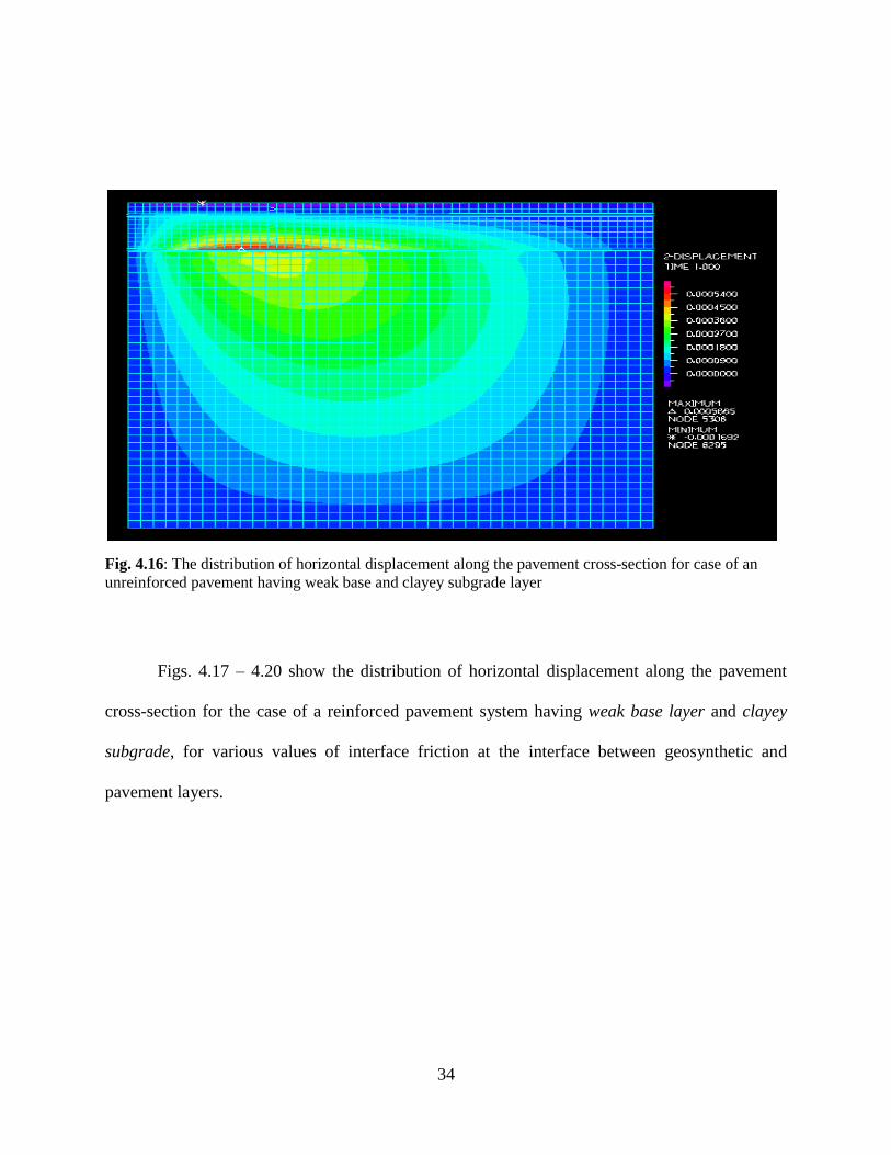
Fig. 4.16: The distribution of horizontal displacement along the pavement cross-section for case of an
unreinforced pavement having weak base and clayey subgrade layer
Figs. 4.17 – 4.20 show the distribution of horizontal displacement along the pavement
cross-section for the case of a reinforced pavement system having weak base layer and clayey
subgrade, for various values of interface friction at the interface between geosynthetic and
pavement layers.

35
Fig. 4.17: The distribution of horizontal displacement along the pavement cross-section for case of a
reinforced pavement µ1=0; and µ2=0 having weak base and clayey subgrade layer
Fig. 4.18: the distribution of horizontal displacement along the pavement cross-section for case of a
reinforced pavement µ1=0.392; and µ2=0.294 having weak base and clayey subgrade layer
36
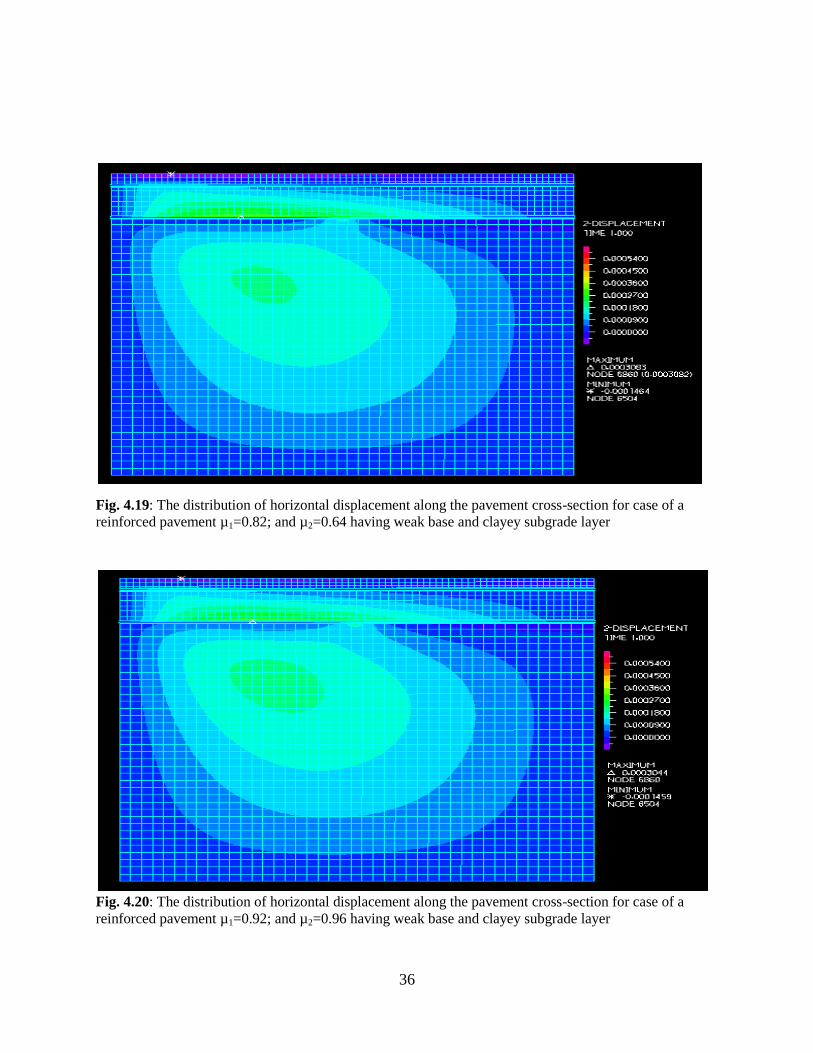
Fig. 4.19: The distribution of horizontal displacement along the pavement cross-section for case of a
reinforced pavement µ1=0.82; and µ2=0.64 having weak base and clayey subgrade layer
Fig. 4.20: The distribution of horizontal displacement along the pavement cross-section for case of a
reinforced pavement µ1=0.92; and µ2=0.96 having weak base and clayey subgrade layer

37
Fig. 4.21 shows the distribution of horizontal displacement along the pavement cross-
section for the case of an unreinforced pavement system having strong base layer and clayey
subgrade layer.
Fig. 4.21: The distribution of horizontal displacement along the pavement cross-section for case of an
unreinforced pavement having strong base and clayey subgrade layer
Figs. 4.21 and 4.22 show the distribution of horizontal displacement along the pavement
cross-section for the case of a reinforced pavement system having strong base layer and clayey
subgrade layer for various values of interface friction.

38
Fig. 4.22: The distribution of horizontal displacement along the pavement cross-section for case of a
reinforced pavement µ1=0; and µ2=0 having strong base and clayey subgrade layer
Fig. 4.23: The distribution of horizontal displacement along the pavement cross-section for case of a
reinforced pavement µ1=0.92; and µ2=0.96 having strong base and clayey subgrade layer

39
Fig. 4.24 shows the distribution of horizontal displacement along the pavement cross-
section for the case of an unreinforced pavement system having weak base layer and silty
subgrade layer.
Fig. 4.24: The distribution of horizontal displacement along the pavement cross-section for case of an
unreinforced pavement having weak base and silty sand subgrade layer
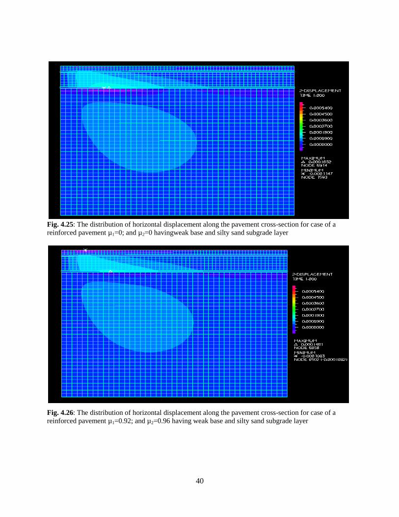
Figs. 4.25 and 4.26 show the distribution of horizontal displacement along the pavement
cross-section for case of a reinforced pavement system having weak base layer and silty sand
subgrade layer for various values of interface friction.
40
Fig. 4.25: The distribution of horizontal displacement along the pavement cross-section for case of a
reinforced pavement µ1=0; and µ2=0 havingweak base and silty sand subgrade layer
Fig. 4.26: The distribution of horizontal displacement along the pavement cross-section for case of a
reinforced pavement µ1=0.92; and µ2=0.96 having weak base and silty sand subgrade layer

41
Fig. 4.27 shows the distribution of horizontal displacement along the pavement cross-
section for the case of an unreinforced pavement system having strong base layer and silty
subgrade layer.
Fig. 4.27: The distribution of horizontal displacement along the pavement cross-section for case of an
unreinforced pavement having strong base and silty sand subgrade layer
Figs. 4.28 and 4.29 show the distribution of horizontal displacement along the pavement
cross-section for case of a reinforced pavement system having strong base layer and silty sand
subgrade layer for various values of interface friction.

42
Fig. 4.28: The distribution of horizontal displacement along the pavement cross-section for case of a
reinforced pavement µ1=0; and µ2=0 having strong base and silty sand subgrade layer
Fig. 4.29: The distribution of horizontal displacement along the pavement cross-section for case of a
reinforced pavement µ1=0.92; and µ2=0.96 having strong base and silty sand subgrade layer

43
It can be concluded from observations of Figs 4.16 to 4.29, that the maximum reduction
in the horizontal displacement occurs when the friction coefficients equal µ1= 0.92; µ2 = 0.96
between the geosynthetic and the foundation layer, and between the geosynthetic and the
subgrade respectively. The influence of the geosynthetic is found to decrease when the strength
of base layer increases.
4.4 Variation of Vertical Surface Deflection
From the variations of the vertical deflection of the surface (1-2) (Figs. 4.2 to 4.15), the
maximum deflections were determined for the various cases and are reported in Table (4.1).
The variation of the maximum vertical surface deflection along surface (1-2) (Fig. 4.1) is shown
in Figs. 4.30, 4.31, 4.32, and 4.33. It is seen from these figures that the highest reduction of
vertical surface deflection in the pavement with weak base layer and weak subgrade layer is
about 17% (Table 4.1). This reduction is reached in the case of full bonding between the
geosynthetic and the granular base, and between the geosynthetic and the subgrade. In addition,
Table (4.1) shows that when the friction coefficient µ between the geosynthetic and the granular
base, and between the geosynthetic and subgrade increases the amount of reduction of the
vertical surface deflection increases up to 14.54% for µ1= 0.92 for contact surface between the
geosynthetic and the foundation layer; and µ2= 0.96 for contact between the geosynthetic and
cohesive soil. Fig (4.30) shows the amount of reduction in vertical surface deflection for
different interface friction values for pavement system of weak base layer and weak subgrade
layer.

44
Table (4.1): Maximum vertical surface deflection (mm)
Max surface deflection (mm)
Weak SG & Weak GB
EFF% Weak SG & Strong GB
EFF% Strong SG &
Weak GB EFF%
Strong SG & Strong GB
EFF%
Unreinforced soil 4.249 0.00 2.600 0.00 1.686 0.00 1.036 0.00
Reinforced; µ1=0, µ2=0
3.700 12.92 2.422 6.85 1.688 -0.12 1.049 -1.25
µ1=0.392, µ2=0.294 3.668 13.67 2.411 7.27 1.674 0.71 1.043 -0.68
µ1=0.82, µ2=0.64 3.645 14.22 2.402 7.62 1.662 1.42 1.037 -0.10
µ1=0.92, µ2=0.96 3.631 14.54 2.397 7.81 1.653 1.96 1.032 0.39
Reinforced; Full Bonding
3.542 16.64 2.357 9.35 1.549 8.13 0.96 7.34

45
0
0.5
1
1.5
2
2.5
3
0 500 1000 1500 2000 2500 3000 3500
surf
ace
def
lect
ion
(m
m)
Horizontal distance from the load centerline (mm)
Unreinforced soil
Reinforced; µ1=0, µ2=0
Reinforced;µ1=0.392,µ2=0.294
Reinforced;µ1=0.92, µ2=0.96
Reinforced;Full-Bonding
0
0.5
1
1.5
2
2.5
3
3.5
4
4.5
0 500 1000 1500 2000 2500 3000 3500
surf
ace
def
lect
ion
(m
m)
Horizontal distance from the load centerline (mm)
Unreinforced
Reinforced;µ1=0, µ2=0
Reinforced;µ1=0.392,µ2=0.294
Reinforced;µ1=0.82,µ2=0.64
Reinforced;µ1=0.92,µ2=0.96
Reinforced;µ1=0.92,µ2=0.96
Reinforced; Full Bonding
Fig. 4.30: The vertical surface deflection along edge (1-2) for pavement system having weak
base layer and weak subgrade layer
Fig. 4.31: The vertical surface deflection along edge (1-2) for pavement system having strong
base layer and weak subgrade layer

46
-0.2
0
0.2
0.4
0.6
0.8
1
1.2
1.4
1.6
1.8
0 1000 2000 3000 4000
Axi
s su
rfac
e d
efle
ctio
n (
mm
)
Horizontal distance from the load centerline (mm)
Unreinforced
Reinforced;µ1=0, µ2=0
Reinforced;µ1=0.392,µ2=0.294
Reinforced;µ1=0.82, µ2=0.64
Reinforced;µ1=0.92, µ2=0.96
Reinforced; Full Bonding
0
0.2
0.4
0.6
0.8
1
1.2
0 500 1000 1500 2000 2500 3000 3500
surf
ace
de
fle
ctio
n (
mm
)
Horizontal distance from the load centerline (mm)
Unreinforced
Reinforced;µ1=0, µ2=0
Reinforced;µ1=0.392,µ2=0.294
Reinforced;µ1=0.82, µ2=0.64
Reinforced;µ1=0.92, µ2=0.96
Reinforced; Full Bonding
Fig. 4.32: The vertical surface deflection along edge (1-2) for pavement system having weak
base layer and silty sand subgrade layer
Fig. 4.33: The vertical surface deflection along edge (1-2) for pavement system having strong
base layer and silty sand subgrade layer

47
It is seen from results reported for the pavement of strong foundation layer and weak
subgrade layer that the amount of vertical surface deflection is 2.6 (mm) for unreinforced
pavement. This amount is decreased when the geosynthetics is placed between foundation layer
and subgrade with the highest reduction reaching 9.4% in the case of full bonding at the contact
surfaces between the geosynthetic and other pavement layers (granular base, subgrade). In
addition, when the friction coefficients of contact surfaces between the geosynthetics and the
foundation layer, and between the geosynthetic and the cohesive soil increase, the amount of
reduction increases to 7.8% for µ1= 0.92 at the contact surface between the geosynthetic and the
foundation layer; and µ2= 0.96 for contact surface between the geosynthetic and the cohesive
soil.
On the other hand, the influence of interface friction coefficients at the contact surfaces
between geosynthetics and the pavement layers (base, and subgrade) on pavement performance
decreases for the pavement of weak foundation layer and strong subgrade layer, with the highest
reduction reaching only 2%. This amount decreases to 0.4% in the pavement with strong
foundation layer and strong subgrade for µ1= 0.92 at the contact surface between the
geosynthetic and the foundation layer; and µ2= 0.96 for contact surface between the geosynthetic
and the cohesive soil.
It can be concluded from these observations that the highest reduction of the vertical
surface deflection occurs when the friction coefficients equal µ1= 0.92; µ2 = 0.96 between the
geosynthetic and the foundation layer, and between the geosynthetic and the subgrade
respectively. Additionally, the influence of the geosynthetic is found to decrease when the
strength of subgrade layer increases.

48
4.5 Variation of Horizontal Displacement
The maximum horizontal displacement along the interface between geosynthetic and
pavement layers is reported in Table (4.2) for the various sections analyzed. The variation of the
maximum horizontal displacement along the interface between geosynthetics and pavement
layers is shown in Figs. 4.34, 4.35, 4.36, and 4.37. Table (4.2) shows that the highest reduction
of horizontal displacement in the pavement of weak base layer and weak subgrade layer is
49.74%. This reduction is reached in the case of full bonding between the geosynthetic and the
granular base layer, and between the geosynthetic and the subgrade layer. In addition, (Table 4.2)
shows that when the friction coefficients µ between the geosynthetic and the granular base and
between the geosynthetic and subgrade increase, the amount of reduction of the horizontal
displacement increases until it reaches 46.4 % for µ1= 0.92 at the contact surface between the
geosynthetic and the foundation layer and µ2= 0.96 for contact surface between the geosynthetic
and cohesive soil layer. The distribution of maximum horizontal displacement along the contact
surfaces between the geosynthetic layer and the pavement layers (base and subgrade layers) is
shown in Fig.4.34 for the pavement system having weak base layer and weak subgrade layer.

49
Table (4.2): Maximum horizontal displacement (mm)
Horizontal displacement (mm)
Weak SG & Weak GB
EFF% Weak SG, Strong GB
EFF% Strong SG &
Weak GB EFF%
Strong SG & Strong GB
EFF%
Unreinforced soil 0.567 0.00 0.265 0.00 0.225 0.00 0.140 0.00
Reinforced; µ1=0, µ2=0
0.323 43.03 0.214 19.25 0.165 26.67 0.132 5.71
µ1=0.392, µ2=0.294
0.315 44.44 0.211 20.38 0.16 28.89 0.129 7.86
µ1=0.82, µ2=0.64 0.308 45.68 0.209 21.13 0.153 32.00 0.127 9.29
µ1=0.92, µ2=0.96 0.304 46.38 0.207 21.89 0.148 34.22 0.125 10.71
Reinforced; Full Bonding
0.285 49.74 0.197 25.66 0.11 51.11 0.103 26.43

0
0.1
0.2
0.3
0.4
0.5
0.6
0 1000 2000 3000 4000
Ho
rizo
nta
l dis
pla
cem
ent
(mm
)
Horizontal distance from the load centerline (mm)
Unreinforced
Reinforced; µ1=0,µ2=0Reinforced;µ1=0.392,µ2=0.294Reinforced;µ1=0.82,µ2=0.64Reinforced;µ1=0.92,µ2=0.96Reinforced; Fullbonding
0
0.05
0.1
0.15
0.2
0.25
0.3
0 1000 2000 3000 4000
Ho
rizo
nta
l dis
pla
cem
ent
(mm
)
Horizontal distance from the load centerline (mm)
Unreinforced
Reinforced;µ1=0, µ2=0
Reinforced;µ1=0.392,µ2=0.294
Reinforced;µ1=0.82,µ2=0.64
Reinforced;µ1=0.92,µ2=0.96
Reinforced; Full Bonding
Fig. 4.34: The horizontal displacement along edge (3-4) for pavement system having weak base
layer and clayey subgrade layer
Fig. 4.35: The horizontal displacement along edge (3-4) for pavement system having strong base
layer and clayey subgrade layer

51
-0.05
0
0.05
0.1
0.15
0.2
0.25
0 1000 2000 3000 4000
Ho
rizo
nta
l dis
pla
cem
ent
(mm
)
Horizontal distance from the load centerline (mm)
Unreinforced
Reinforced;µ1=0,µ2=0
Reinforced;µ1=0.392, µ2=0.294
Reinforced;µ1=0.82, µ2=0.64
Reinforced;µ1=0.92, µ2=0.96
Reinforced; FullBonding
-0.02
0
0.02
0.04
0.06
0.08
0.1
0.12
0.14
0 1000 2000 3000 4000
Ho
rizo
nta
l dis
pla
cem
ent
(mm
)
Horizontal distance from the load centerline (mm)
Unreinforced
Reinforced;µ1=0, µ2=0
Reinforced; µ1=0.392,µ2=0.294
Reinforced; µ1=0.82,µ2=0.64
Reinforced; µ1=0.92,µ2=0.96
Reinforced; FullBonding
Fig. 4.36: The horizontal displacement along edge (3-4) for pavement system having weak base
layer and silty sand subgrade layer
Fig. 4.37: The horizontal displacement along edge (3-4) for pavement system having strong base
layer and silty sand subgrade layer

52
It is also observed that for the pavement of strong foundation layer and weak subgrade
layer that the amount of horizontal displacement decreases when the geosynthetic is placed
between the base and subgrade layers. The amount of decrease is dependent on the amount of
friction coefficients between the geosynthetic layer and the pavement layers (base and subgrade).
For example, when µ= 0 between two contact surfaces of geosynthetics and pavement layers
(base and subgrade) the amount of horizontal displacement reached 0.214 (mm), while it reaches
0.207 (mm) when µ1= 0.92, and µ2= 0.96; between the geosynthetic and the foundation layer,
and between the geosynthetic and subgrade respectively as shown in Table (4.2).
On the other hand, the influence of geosynthetic on the pavement performance increases
for pavements with weak foundation layer and strong subgrade layer, with the highest reduction
reaching 51.1% .This reduction is reached for the case of full bonding between the geosynthetic
and the granular base layer, and between the geosynthetic and the subgrade layer. In addition,
Table (4.2) shows that when the friction coefficient µ between the geosynthetics and the granular
base and between the geosynthetics and subgrade increases the amount of horizontal
displacement reduction increases to 34.2% for µ1= 0.92 at the contact surface between the
geosynthetic and the foundation layer; and µ2= 0.96 for contact surface between the geosynthetic
and cohesive soil Fig (4.34). In contrast, the amount of reduction of the horizontal displacement
decreases for the pavement of strong foundation layer and strong subgrade layer to 0.125 (mm)
for µ1= 0.92; µ2= 0.96, while reaches 0.14 (mm) for unreinforced pavement Fig. 4.35. These
observations show that the maximum horizontal displacement occurs at the contact surface
between foundation layer and cohesive soil layer in the unreinforced pavement and the
geosynthetic reinforced pavement.

53
In addition, the maximum reduction in the horizontal displacement occurs when the
friction coefficients equal µ1= 0.92; µ2 = 0.96 between the geosynthetic and the foundation layer,
and between the geosynthetic and the subgrade respectively. Also, the influence interface friction
coefficients at the contact surfaces between the geosynthetics and the pavement layers decreases
when the strength of base layer increases.
4.6 Comparison of Results
The results obtained in this study are compared with the results of past studies. The
comparison shows that good agreement is obtained concerning the following observations: 1) the
strength of subgrade has a significant effect on the performance of the reinforcement pavement.
The influence of geosynthetics as a reinforcement material is beneficial for weak subgrade
foundation (Nazzal et al. 2006, Wathugala et al. 1996 and Saad et al. 2006); 2) the reduction of
vertical surface deflection is also dependent on the strength of subgrade layer and the strength of
foundation layer, geosynthetic stiffness, and the thickness of the foundation layer Nazzal et al.
(2006). In this study, the effect of subgrade stiffness and the foundation layer stiffness have been
investigated. It was found that the reduction of vertical surface deflection reaches to (16%), this
is close to the other studies’ results, refer to Saad et al. (2006), Wathugala et al. (1996), and
Dondi (1994) which found the reduction of vertical surface deflection will be in range (14% -
34%).

54
CHAPTER FIVE
CONCLUSIONS AND RECOMMENDATIONS
5.1 Conclusions
A series of finite element simulations were conducted to investigate the benefits of using
geosynthetics in pavement sub layers for different cases of base course and subgrade; weak
versus strong. The results of these simulations have provided insights into the effects of the
interface friction coefficient between geosynthetic and base courses on vertical surface deflection
and horizontal displacement of layers, as summarized below:
1) The highest reduction of the vertical surface deflection is observed for pavement with
weak base and weak subgrade layer. This reduction, which reaches nearly 14.5% is
achieved when the friction coefficients of the interface reach to µ1 = 0.92 and µ2 = 0.96,
respectively. Note that these values were recommended by Koerner (1994). In addition,
the amount of reduction on the vertical surface deflection for a reinforced pavement
structure is found to decrease when the strength of subgrade increases to reach 2% for the
pavement system having strong subgrade and weak granular base.
2) The strength of the base layer has a significant effect on horizontal displacement. The
highest reduction of the horizontal displacement is reached for the pavement with weak
granular base and weak subgrade. This reduction, which reaches 46%, is achieved when
the friction coefficients of the interface reach to µ1 = 0.92 and µ2 = 0.96, respectively.
Such influence is found to reduce when the stiffness of the granular base increased.

55
It is evident from these studies that the interface friction between the geosynthetics and
the pavement layers (base and subgrade) affected the performance of the pavement structure
the most. The best results can be achieved when the friction coefficients of the interface
equal µ1 = 0.92 and µ2 = 0.96, confirming the observations made by Koerner (1994).
5.2 Recommendations
The numerical analyses here were conducted to study the performance of reinforced and
unreinforced pavement cross-section under monotonic loadings. It is recommended to extend
the study to cyclic loadings. While the effects of interface friction between the geosynthetic
and soil layers on reinforced pavement performance is highlighted by this study using
parametric studies, it would be of use to quantify the actual values in the future for the
various geosynthetics and soils. It is also recommended to use the concept of interface
interlocking and shear strength towards the purpose.

56
References
Adina R&D Inc. (Adina R&D). (2001). “Finite element computer program, theory and modeling guide.”
Rep. ARD 01-7, Vol. 1, Adina R&D Inc., Watertown, Mass.
Barksdale, R. D., Brown, S. F., and Chan, F., (1989). "Potential benefits of geosynthetics in flexible
pavement systems." National cooperative highway research report No.315, TRB national
Research Council, Washington, DC, 1-53.
BOSTD Geosynthetics., (2007). “Soil-geogrid friction coefficients.” pp 2.1-2.5
http://www.newgrids.com/userImages/00000126_Design%20Factors%20Section%202%20Fricti
on.pdf
Brocklehurst, J.C., (1993). “Finite element studies of reinforced and unreinforced two-layer soil system.”
A Thesis Ssubmitted for the Degree of Doctor of Philosophy at the University of Oxford.
Brown, S.F., Brunton, J.M., Hughes, D.A.B., and Brodrick, B.V., (1985). “Polymer grid reinforcement of
asphalt.” Proc., Assoc. of Asphalt Paving Technologists, 54, 18-41.
Chen, W, F., and Baladi, G, Y., (1985). “Soil plasticity; Theory and implementation.” Elsevier Science
Cho, Y., McCullough, B. F., and Weissmann, J., (2000). "Consideration on finite-element method
application in pavement structural analysis." Transportation Research Record 1539, TRB
national Research Council, Washington, DC , 96-101.
Collins, I, F., (2005). “The concept of stored plastic work or frozen elastic energy in soil mechanics.”
Geotechnique, 55. 373-382
Davies, M.C.R. and Bridle, R.J., 1990, “Predicting the Permanent Deformation of Reinforced Flexible
Pavement Subject to Repeated Loading.” Performance of Reinforced Soil Structures, 421-425.
Desai, C, S., and Siriwardane, H, A., (1984). "Constitutive laws for engineering material." Prentice-
Hall,Englewood cliffs, N. J.
Desai, C, S., Somasundaram, S., Frantziskonis, G, N., and Hierarchical, A., (1986). "Approach for
constitutive modeling of Geologic materials." International Journal for Numerical and Analytical
Methods in Geomechanics, 10. 225-257
Diambra, A., Ibraim, E., Muir Wood, D., and Russell, A, R., (2010). "Fibre reinforced sands: Experiments
and modeling." Geotextiles and geomembranes, 28, 238-250.
Dondi, G., (1994). “Three-dimensional finite element analysis of a reinforced paved road." Fifth
international conference on geotextiles, geomembranes and related products Singapore, 1, 95-
100.

57
Haas, R., Walls, J., and Carroll, R.G., (1988). "Geogrid reinforcement of granular bases in flexible
pavements." Transportation Research Record 1188, 19-27.
Hausmann, M, R., (1990). “Engineering principles of ground modification.” McGraw-Hill.
Holtz, R, D., Christopher, B, R., and Berg, R, R., (1998). "Geosynthetic design and construction
guidelines." Federal highway administration, Washington DC, FHWA/HI-98/038. 460p
Howard, I., and Warren, K., (2006). "Finite element approach for flexible pavements with geosynthetics."
GeoCongress 2006-ASCE. 187-192
Juran, I., Guermazi, A., Chen, C.L., and Ider, M.H., (1988). "Modelling and simulation of load transfer in
reinforced soils: part 1." International Journal for Numerical and Analytical Methods in
Geomechanics, 12, 141-155.
Juran, I., Ider, M, H., Chen, C.L., and Guermazi, A., (1988). "Numerical analysis of the response of
reinforced soils to direct shearing: Part 2." International Journal for Numerical and Analytical
Methods in Geomechanics, 12, 157-171.
Koerner, R, M., (1994). “Designing with geosynthetics; Third edition.” Prentice-Hall, Inc.
Ling, H, I., and Liu, K., (2003). "Finite element studies of asphalt concrete pavement reinforced with
geogrid ." Engineering mechanics-ASCE, 129. 801-811
Ling, H, I., and Liu, Z., (2001). "Performance of geosynthetic-reinforced asphalt pavements."
Geotechnical and geoenviromental engineering. 177-184
Nazzal, M, D., Abu-Farsakh, M, Y., and Mohammad, L, N., (2006). "Numerical analysis of geogrid
reinforcement of flexible pavements." GeoCongress 2006-ASCE. 1-6
Penner, R., Haas, R., Walls, J., and Kennepohi, G., (1985). "Geogrid reinforcement of granular bases."
Paper presented at the Transportation Association of Canada Annual Conference, Vancouver,
British Columbia, Canda.
Perkins, S.W., (1999). “Mechanical response of geosynthetic-reinforced flexible pavements: Technical
paper.” Geosynthetics international, 6. 347-381
Perkins, S.W., (2001). “Numerical modeling of geosynthetic reinforced flexible pavement: Final report.”
Rep. No. FHWA/MT-01/003/99160-2, Montana Department of Transportation, Helena, Mont.
Perkins, S.W., and Ismeik, M., (1997). “A synthesis and evaluation of geosynthetic-reinforced base layers
in flexible pavements: part 2.” Geosynthetics International. 4, 605-621.
Rowe, R, K., and Skinner, D, G., (2001). "Numerical analysis of geosynthetic reinforced retaining wall
constructed on a layered soil foundation." Geotextiles and geomembranes , 19. 387-412

58
Saad, B., Mitri, H., and Poorooshasb, H., (2006). "3D FE analysis of flexible pavement with geosynthetic
reinforcement." J. Transportation Engineering 132, 402-415.
Wang, J., Dove, J, E., and Gutierrez, M, S., (2007). "Anisotropy-base failure criterion for interface
systems." Geotechnical and geoenviromental engineering, 133. 599-608
Wathugala, G, W., and Desai, C, S., (1993). "Constitutive model for cyclic behavior of clay I: Theory."
Geotechnical engineering, 119. 714-729
Wathugala, G.W., Huang, B., and Pal, S., (1996). "Numerical simulation of geosynthetic reinforced
flexible pavement." Transportation Research Record 1534, TRB national Research Council,
Washington, DC , 12, 58-65.
Yan, Q., Mei, Y., Li, C., and Deng, W., (2010). "Study on the characteristics of geogrids / soil interface."
Mechanic Automation and Control Engineering (MACE), 2010 International Conference, 1241 -
1248.
Zornberg, J.G. (2011). “Advances in the use of geosynthetics in pavement design." Geosynthetics India,
11, 3-21.


