Buyer-Seller Relationships in International Trade: Do Your Neighbors Matter?1

Fariha Kamal2 Center for Economic Studies

U.S. Census Bureau 4600 Silver Hill Road

Washington, DC 20233, U.S.A fariha.kamal@census.gov

+1 (301) 763 4575

Asha Sundaram School of Economics

University of Cape Town Rondebosch, Cape Town 7701

South Africa assundar.wk@gmail.com

+27 (1) 72 781 1813

August 15, 2013

Abstract

An exporter needs to locate an importer in order to conduct an international trade transaction. In this paper, we investigate if the presence of other exporters in the neighborhood of a firm, selling to a particular foreign buyer, facilitates a match between the firm and this buyer. In particular, we search for evidence of importer-specific spillovers in the decision of Bangladeshi textile manufacturers to sell to a U.S. importer using the universe of U.S. import transactions with Bangladesh in textile products. We find that the presence of neighboring exporters selling to a U.S. importer increases the likelihood of exporting to that U.S. importer. Results suggest that importer-specific spillovers account for a significant portion of destination-specific export spillovers previously documented in the literature. We also find that these spillovers vary by both importer and exporter characteristics. Our study highlights the significance of spillovers from exporting, whose scope extends beyond the level of the export destination, to that of the importing firm. This suggests that knowledge and information gains are potentially realized at a disaggregated level, where the individual importer and exporter interact. JEL Classification: F1, R12, L25 Keywords: importer-specific spillovers, export decision, trading pairs

1 Any opinions and conclusions expressed herein are those of the authors and do not necessarily represent the views of the U.S. Census Bureau. All results have been reviewed to ensure that no confidential information is disclosed. We thank Emin Dinlersoz and participants at the Center for Economic Studies seminar series for helpful comments. 2 Corresponding author.

2

1. Introduction

International trade involves numerous transactions between buyers and suppliers across

borders. A foreign transaction is the result of a firm in one country trading with another firm

located in a foreign country. Therefore, it is important to understand the factors influencing

buyer and seller relationships in international trade. A large literature looks at the determinants

of exporter status and highlights the role of export spillovers that improve the likelihood of firms

exporting to foreign destinations (Koenig, 2009; Koenig, Mayneris, and Poncet, 2010; Bernard

and Jensen, 2004). These studies find that greater presence of exporters to a specific foreign

destination close to a firm can increase the likelihood that the firm exports to the same

destination.3 However, to the best of our knowledge, there is no existing empirical evidence on

importer-specific spillovers.

We fill this gap by looking at how the presence of exporters neighboring a firm and

exporting to a particular foreign buyer, impacts the likelihood that the firm will export to the

same buyer. Hence, our focus is on the match between the importing and exporting firm, the

micro units at which international trade occurs. Our study differs from earlier studies in this area

in a crucial way. Previous analyses focus on spillovers from information sharing or cost sharing

while exporting to a destination country. The idea here is that the presence of exporters nearby

exporting to the same destination can facilitate knowledge of business norms and culture, of

setting up foreign exchange accounts or service centers abroad, or of retaining customs agents,

and hence lower the costs of exporting. In our paper, we ask if these spillovers are specific to the

3 Bernard and Jensen (2004) consider the role of both geographic and sectoral spillovers in the export decision of a U.S. plant and find no role for spillovers in determining a plant’s export status. Therefore, it differs in two main ways from Koenig (2009) and Koenig, Mayneris, and Poncet (2010) who consider the role of export spillovers on the decision of French firms to export to a particular country - the spillovers considered are not destination specific and geography is at the state level that is much more aggregated than the employment areas in France.

3

buyer. Thus, our paper is a step further in the direction of isolating the nature of export

spillovers and the channels through which they operate. By looking at the formation of buyer –

supplier matches across borders, our paper also relates to the nascent body of work exploring

buyer-seller matches in international trade (Eaton, Eslava, Jinkins, Krizan, Tybout, 2013 and

Monarch, 2013).

Importer-specific spillovers can operate through various channels. The presence of

exporting firms in the neighborhood selling to the same buyer can facilitate information sharing

about exporting to that particular buyer. This might include knowledge of any needs of the

importer that require customization such as the buyer’s product specifications, custom packaging

requirements, and its clienteles’ tastes and preferences. Additionally, there may be cost sharing,

where costs might include search costs of locating a buyer, investing in activities that promote an

exporter’s product to a potential buyer such as advertising or participating in trade shows etc.

The ability to obtain tacit knowledge and share in costs is likely to lower the fixed and/or

variable costs of exporting.

Numerous studies in the literature look at destination-specific export spillovers. Koenig

(2009) and Koenig et al (2010) use data on French exporters to find that greater presence of

exporters nearby affects the decision to start exporting, but not the volume of exports. Hence,

the authors infer that export spillovers affect the fixed, but not the variable cost of exporting.

Koenig et al (2010) also find that spillovers exhibit spatial decay. Fernandes and Tang (2012)

find that for Chinese exporters, new exporters’ first-year sales and probability of survival are

higher in cities where there are existing exporters selling to the same export destination–industry.

They also find that spillovers are heterogeneous across firm types. Spillovers from processing

4

exporters are weaker compared to those engaged in ordinary exports and foreign exporting firms

located in China benefit less than their domestic counterparts.

In addition to contributing to the international trade literature, we also shed light on a

specific mechanism of urban agglomeration economies. The theoretical literature explaining the

existence of urban agglomeration economies posits that larger markets allow for a better match

between buyers and suppliers (Duranton and Puga, 2004), however, empirical evidence is scant.

Most of the empirical work examining the matching mechanism has focused on matches between

employers and employees and Puga (2010) concludes that “[o]n the empirical side, evidence of

matching as a source of agglomeration is perhaps most needed” (p. 216). In light of this, our

work can be considered as taking a significant step towards establishing the empirical association

between agglomeration economies and better matches between buyers and suppliers, albeit

across national borders.

By looking at the match between a buyer and a seller, we highlight the scope of spillovers

beyond information sharing on country-specific transaction costs, or cost sharing in exporting to

the destination country, to information and cost sharing to export to a particular buyer. Thus, we

relate the presence of exporters neighboring exporter , selling to an importer , on the decision

of exporter to start exporting to importer , as well as the continuing trading status of an

exporter-importer pair. We use transaction level data on U.S. imports in textile products from

Bangladeshi exporters, sourced from the U.S. Census Bureau. Focusing on trade transactions in

textile products between the U.S. and Bangladesh is motivated by the need to construct our

analysis dataset fairly easily while focusing on an important bilateral trade relationship.4

4 See Section 3 for further detail on data construction.

5

Bangladesh is the fourth largest apparel exporter in the U.S.5 Over three quarters of Bangladeshi

exports are in textile and apparel products with U.S. being the second largest export destination

(Tables 4 and 5, Trade Policy Review, 2012). Exporters in our sample are Bangladeshi textile

manufacturing firms, while importers are U.S. firms operating in all sectors of the economy

including manufacturing, wholesale, and retail.

We estimate a linear probability model with exporter-year and importer fixed effects as

well as time-varying importer controls. The results indicate that a one percent increase in the

number of exporters in the city selling to the same importer results in a 0.34% increase in the

likelihood of matching with the same buyer for the first time; and a 0.19% increase in the

likelihood of a match with the same buyer at any point in time. We also find that spillover

effects differ by both exporter and importer characteristics. Spillovers are strongest for smaller

exporters compared to those that have higher average export sales. This suggests that smaller

exporters may not have the internal resources of larger exporters that facilitate buyer-seller

relationships and therefore importer-specific spillovers are associated with higher likelihood of

matching with U.S. buyers that transact with neighboring exporters. We further find that

spillovers are stronger when the importer is small relative to when the importer is large. This

suggests that U.S. importers vary in their behavior to procure and maintain supplier relationships.

The rest of the paper is organized as follows. Section 2 presents our empirical model and

identification strategy. Section 3 describes the data and measurement of key variables. Section

4 discusses the empirical findings and the final section concludes.

2. Empirical model and strategy

5 See http://www.bdembassyusa.org/uploads/US%20-%20BD%20trade.pdf.

6

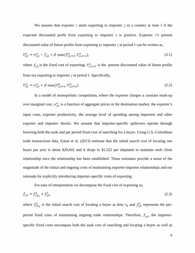
We assume that exporter starts exporting to importer in a country at time if the

expected discounted profit from exporting to importer is positive. Exporter ’s present

discounted value of future profits from exporting to importer at period can be written as,

, (2.1)

where is the fixed cost of exporting; is the present discounted value of future profits

from not exporting to importer at period . Specifically,

. (2.2)

In a model of monopolistic competition, where the exporter charges a constant mark-up

over marginal cost, is a function of aggregate prices in the destination market, the exporter’s

input costs, exporter productivity, the average level of spending among importers and other

exporter and importer shocks. We assume that importer-specific spillovers operate through

lowering both the sunk and per period fixed cost of searching for a buyer. Using U.S.-Colombian

trade transactions data, Eaton et al. (2013) estimate that the initial search cost of locating one

buyer per year is about $20,642 and it drops to $1,522 per shipment to maintain each client

relationship once the relationship has been established. These estimates provide a sense of the

magnitude of the initial and ongoing costs of maintaining exporter-importer relationships and our

rationale for explicitly introducing importer-specific costs of exporting.

For ease of interpretation we decompose the fixed cost of exporting as,

, (2.3)

where is the initial search cost of locating a buyer at time and represents the per-

period fixed costs of maintaining ongoing trade relationships. Therefore, , the importer-

specific fixed costs encompass both the sunk cost of searching and locating a buyer as well as

7

per period fixed costs of investing in activities that promote an exporter’s product to a potential

buyer such as advertising or participating in trade shows, learning about customized packaging

requirements and the importer’s clientele and tastes. We think of these importer-specific costs as

a subset of destination-specific fixed costs that more broadly include learning about local

business norms and culture, retaining a customs agent and lawyers, creating and maintaining a

foreign sales office, establishing foreign currency accounts, etc.

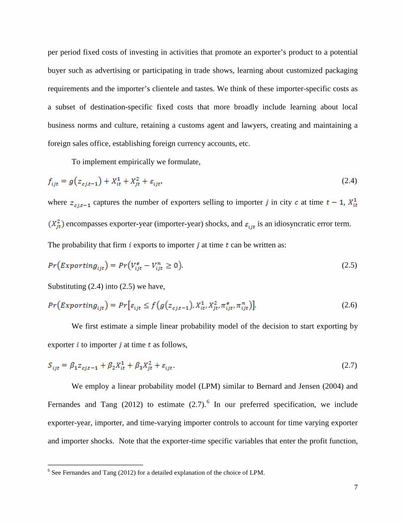
To implement empirically we formulate,

, (2.4)

where captures the number of exporters selling to importer in city at time ,

encompasses exporter-year (importer-year) shocks, and is an idiosyncratic error term.

The probability that firm exports to importer at time can be written as:

. (2.5)

Substituting (2.4) into (2.5) we have,

. (2.6)

We first estimate a simple linear probability model of the decision to start exporting by

exporter to importer at time as follows,

. (2.7)

We employ a linear probability model (LPM) similar to Bernard and Jensen (2004) and

Fernandes and Tang (2012) to estimate (2.7).6 In our preferred specification, we include

exporter-year, importer, and time-varying importer controls to account for time varying exporter

and importer shocks. Note that the exporter-time specific variables that enter the profit function,

6 See Fernandes and Tang (2012) for a detailed explanation of the choice of LPM.

8

like exporter productivity, are absorbed by the exporter–time specific effect. The exporter–time

fixed effects also account for unobserved exporter–specific shocks that determine exporter

status.7 The variable captures spillovers from the presence of exporters to the same buyer

in exporter ’s area . As discussed earlier, these spillovers operate through the sunk and per-

period fixed-costs of exporting. We hypothesize that for first-time matches, importer-specific

spillovers lower the initial sunk cost of locating a buyer and initiating the first-time matches.

is an idiosyncratic error term.

We next estimate a simple linear probability model of the exporting status of exporter to

importer at time as a function of other exporters selling to importer in an area at time

as follows,

. (2.8)

Here, we posit that spillovers operate by further lowering the per-period fixed cost of

maintaining each client relationship in every period. In both (2.7) and (2.8) we expect to be

positive. A priori, we also expect that spillovers will be larger for all matches compared to first-

time matches only since (2.8) includes first-time matches as well. However, we can compare

in (2.7) and (2.8) to get a sense of the relative importance of the channels via which spillovers

operate.

In both specifications (2.7) and (2.8), importer fixed effects control for time-invariant

importer characteristics that may influence the decision to buy from a particular Bangladeshi

7 Since we are using U.S. import transaction records, we only observe the product and value associated with the exporter’s transaction with a U.S. importer. We do not observe exporter characteristics that may influence the decision to export to a U.S. importer such as total factor productivity, total wages, total employment, etc. Therefore, exporter-year fixed effects control for all time varying exporter characteristics that may influence export behavior.

9

exporter.8 This may include factors like firm ownership or state level programs aimed at

increasing exports of local firms by providing matching services with foreign buyers, as long as

these programs do not change over the time period of our analysis.

After controlling for exporter-year and importer fixed effects, we still leave out the

determinants of export behavior that vary across city-importer and time. For instance, if there are

efforts by local governments or trade associations to promote textile exports to particular U.S.

importers within a city, or if particular U.S. importers have preferences for trade with exporters

in particular Bangladeshi cities due to reasons that cannot be observed, then the coefficient on

our own-city spillover variable may not be consistently estimated. To a certain extent, this

endogeneity problem is mitigated since we use a lagged measure of exporter spillovers, thus

circumventing spurious correlation with any contemporaneous city-importer-specific unobserved

factors. Standard errors in all our specifications are clustered at the importer-city level.

3. Data

3.1. Source

The data for this study are drawn from the Linked/Longitudinal Foreign Trade

Transactions Database (LFTTD). The LFTTD is a transaction-firm linked database linking

individual trade transactions, both export and imports, to the U.S. firms that make them.9 The

dataset contains information on the value, quantity, and date of transaction of a ten-digit

Harmonized Commodity Description and Coding system (commonly called Harmonized System

or HS) products. The Harmonized System is an internationally standardized system of names

and numbers for classifying traded products. The LFTTD also contains information about the

8 All our results remain qualitatively unchanged with the inclusion of importer-year fixed effects. 9 See http://www.census.gov/ces/dataproducts/datasets/lfttd.html for more information.

10

trading parties. We focus on the universe of all U.S. import transactions (LFTTD-IMP) that

occurred between 2002 and 2009. In particular, we consider all import transactions of textile

products from Bangladesh aggregated at the exporter-importer and year level. Although, the

LFTTD-IMP spans the years 1992 through 2009, we have chosen to focus on the most recent

eight-year period for ease of constructing the analysis dataset.10

We focus on U.S. textile imports because we want to investigate the export behavior of

goods producers and not trade intermediaries. In the case of trade intermediaries, we are worried

that the actual match might potentially have occurred between the producer, who we cannot

observe, and the U.S. importer, while the intermediary observed by us as shipping the data has

no role in the matching process. The identifier for the exporter in the U.S. import transactions

database is the manufacturer in case of textile products (see details below), and we exploit this

useful feature of the data to circumvent this issue. In addition, we selected Bangladesh for two

main reasons. First, textile exports account for close to 80% of total Bangladeshi exports over the

sample period and this allows us to capture a significant portion of economic activity of this U.S.

trading partner. Second, we wanted to choose a trading partner that is a major player within the

textile sector but still allows us to construct our dataset with ease as explained in the following

section.

3.2. Dataset Construction

We utilize two sets of firm identifiers in the LFTTD-IMP. The first identifies the U.S.

firm (importer) and the second identifies the Bangladeshi textile manufacturer (exporter). The

exporter is uniquely identified by the “Manufacturer ID” (MID), a required field on Form

7501.11 The MID identifies the manufacturer or shipper of the merchandise by an alpha-numeric

10 At the time we began the study, 2009 was the latest available year. 2010 and 2011 have since become available. 11 See form http://forms.cbp.gov/pdf/cbp_form_7501.pdf.

11

code that is constructed using a pre-specified algorithm with a maximum length of 15 characters

(see Appendix for stylized examples).12 For textile shipments, the MID represents the

manufacturer only in accordance with Title 19 Code of Federal Regulations.13 Therefore, our

data captures Bangladeshi textile manufacturers who export directly to the U.S., rather than

intermediaries who may or may not engage in production activities. The particular algorithm

required to construct the MID also circumvents concerns about capturing multi versus single

plant exporters since it is crucial to identify the establishment where the export originates in the

analysis of local exporting spillovers. The last three characters in the MID designate the city

where the manufacturer is located. Therefore, each manufacturer is assigned a MID that uniquely

identifies its location.

We perform several basic data checks. First, we exclude transactions between related

parties.14 Over the sample period, only about 2% of the total value of imports of textile products

between the U.S. and Bangladesh occurs between related parties. Since we are interested in

exploring the role of agglomeration on an exporter’s decision to begin and continue selling to an

importer, we do not want to include trade transactions between the headquarters and subsidiaries

of multinational firms. Next, we exclude transactions where the importer or exporter identifiers

are missing or where the MID does not conform to the algorithm outlined in the CBP Form 7501

Instructions. Examples include a MID that begins or ends with numeric characters or the MID is

a series of numbers.

12 See Block 13 (pg. 7) for description of MID and Appendix 2 (pg. 30) for instructions on constructing MID at http://forms.cbp.gov/pdf/7501_instructions.pdf. 13 See http://www.gpo.gov/fdsys/pkg/CFR-2011-title19-vol1/pdf/CFR-2011-title19-vol1-sec102-23.pdf. 14 “Related party” trade refers to trade between U.S. companies and their foreign subsidiaries as well as trade between U.S. subsidiaries of foreign companies and their foreign affiliates. For imports, firms are related if either owns, controls, or holds voting power equivalent to 6 percent of the outstanding voting stock or shares of the other organization (see Section 402[e] of the Tariff Act of 1930).

12

Once the basic data checks are complete, we construct firm trading pairs using the

importer and exporter firm identifiers for each year in the sample. There are 2,329 and 8,104

unique number of importers and exporters, respectively, over the sample period that results in

18,874,216 possible trading pairs in any single year.15 The final analysis dataset consists of

observations at the importer-exporter pair and year level.

In order to explore heterogeneity in spillovers by importer characteristics, we further

categorize U.S. importers into two size bins – firms that employ less than 250 workers and firms

that employ 250 workers or more. There are 2,329 U.S. importers in our sample and we link

2,306 of these to the Longitudinal Business Database (LBD) to obtain information on firm

employment, age, sector, and multi or single-unit status. The LBD consists of data on all private,

non-farm U.S. establishments in existence that have at least one paid employee, including non-

manufacturing establishments (Jarmin and Miranda, 2002). For multi-units or firms with

multiple plants, age is calculated as the difference between the year of interest and the year of

establishment of its oldest plant. Since multi-unit firms may operate in several sectors of the

economy, the firm is considered to be operating in the sector where the largest share of its

employment is housed.16 Since the LBD is an establishment level dataset, employment is first

aggregated up to the firm level by sector. The firm is then assigned its “predominant” sector and

its employment is aggregated to the firm level.17

3.3. Variables

We consider two independent variables. The first is , a dummy variable that takes on

a value of 1 for the first year that exporter starts selling to importer and 0 otherwise. For

15 This illustrates why we focus on a particular sector and trading partner. The need to construct all possible trading pairs precludes considering all U.S. import transactions. 16 If instead payroll information is used to assign sectors, the categorization remains qualitatively unchanged. 17 Sales data are not readily available for all firms in the sample. Therefore, employment is used to assign a sector.

13

instance, if we observe ABC Garments Company in Bangladesh exporting to XYZ Corporation

in the U.S. from 2003 through 2007, takes on value of 1 in 2003 and all other observations in

the subsequent years are dropped from the data. The second independent variable of interest is

, a dummy variable that takes on a value of 1 if exporter exports to importer in year and

0 otherwise. captures the status of a trading pair in a given year. For instance, in the

preceding example, takes on a value of 1 for 2003 through 2007 and 0 in all other years in

the sample.

The spillover variables, our main dependent variables of interest, refer to other exporters

selling to importer located in the same area as exporter . The geographic area we consider is

the city. The last three characters of the MID designates the city the manufacturer operates in.

We verified the list of cities in our analysis sample against a list of all cities in Bangladesh.

Bangladesh is divided into seven administrative divisions that are further divided into 64 districts

(zila) and within districts, there are 1,009 sub-districts (upazila).18 The city information extracted

from the MID approximately conform to sub-districts.

Sub-districts are analogous to counties in the U.S. and are the second lowest tier of

regional administration. Bangladesh is a small country with an area of about 57,000 square

miles, roughly the size of the state of Iowa, therefore average area of a sub-district is about 56

square miles.19 Figure A1 shows a map of the sub-districts of Bangladesh. There are 282 cities in

our analysis sample. Our main variable of interest is measured as the number of other exporters

selling to importer in the same city as exporter . The spillover variable is lagged one year in

18 See list of geo codes at http://www.bbs.gov.bd/WebTestApplication/userfiles/Image/geocodeweb.pdf. 19 The spillover measures in Koenig (2009) and Koenig et al (2010) are measured at the level of the French employment area that is on average 937 square miles. Therefore, our geographic unit is much smaller and we can expect to capture very localized effects.

14

our econometric specifications and will be referred to as “# exporters-importer j, same city” in

the tables.

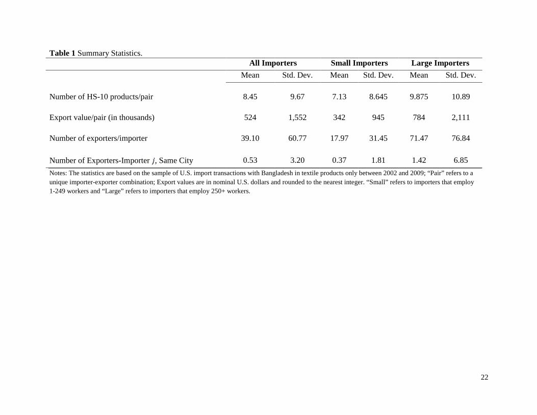
Table 1 presents summary statistics for the entire sample as well as differentiated by

small and large U.S. importers. We find that the total number of HS ten-digit products

transacted, the average export value, number of sellers per buyer and our spillover variable of

interest are larger for exporters selling to large U.S. importers relative to those selling to smaller

U.S. importers. For instance, a trading pair transacts an average of 8 HS ten-digit products over

the sample period and this number increases to about 10 with large importers and is about 7 with

small importers.

4. Results

4.1 Spillover effects on matching between importers and exporters

Table 2 presents results for equation (2.7). We look at the impact of the presence firms

exporting to the same buyer in the neighborhood, defined by a city, of the exporter on the

probability of a first-time match between the importer and the exporter, successively adding

exhaustive fixed effects in each column. Column (1) includes year fixed effects only; column (2)

includes exporter-year and importer fixed effects; and column (3) additionally includes time-

varying importer controls of age and employment. We focus on results from column (3) in our

discussion below as it contains the most exhaustive set of controls, although results are very

similar across the three specifications.

We find that, controlling for exporter–time and importer specific factors that might

determine matches as well as importer age and employment, spillovers are positively associated

with the likelihood of a first–time match. Particularly, we find that an additional exporter in the

15

city selling to the same importer is associated with an increase of 0.00007 in the likelihood of a

first-time match between a Bangladeshi exporter and a U.S. importer. Our coefficient is

statistically significant at the one percent level. In elasticity terms, our results in column (2)

indicate that a one percent increase in the number of exporters in a city selling to a buyer results

in a 0.51% increase in the likelihood of a match with the same buyer for the first time.20 This

figure drops to 0.19% after we account for buyer fixed effects and controls.

Next, we estimate equation (2.8) and present results in Table 3. We ask if spillovers from

neighboring exporters selling to a particular importer are associated with a greater likelihood of

exporting to the same importer. As before, in column (1) we include year fixed effects only;

column (2) includes exporter-year and importer fixed effects; and column (3) additionally

includes time-varying importer controls of age and employment. Under all specifications, we

find that greater presence of firms exporting to an importer in the same city is positively

associated with a higher likelihood of exporting to the same importer. The effect is highly

statistically significant. Focusing on column (3), we find that an additional exporter in the city

exporting to a U.S. importer increases the likelihood of exporting to the same importer by

0.0002. In elasticity terms, our results in column (2) indicate that a one percent increase in the

number of exporters in a city selling to a buyer results in a 0.68% increase in the likelihood of a

match with the same buyer. This figure drops to 0.34% once we account for buyer fixed effects

and controls.

As discussed in Section 2, comparing the coefficients on our spillover coefficient in

Tables 2 and 3 gives us a sense of the relative importance of the channels via which spillovers

operate. Roughly, the coefficient on importer-specific spillovers for first-time matches only is

about half of the coefficient on importer-specific spillovers for all matches. This suggests that 20 Elasticities are calculated using the “margins” command in STATA.

16

importer-specific spillovers are especially beneficial in lowering the initial search costs that can

be more than thirteen times higher than per period fixed costs as indicated by estimates in Eaton

et al (2013).

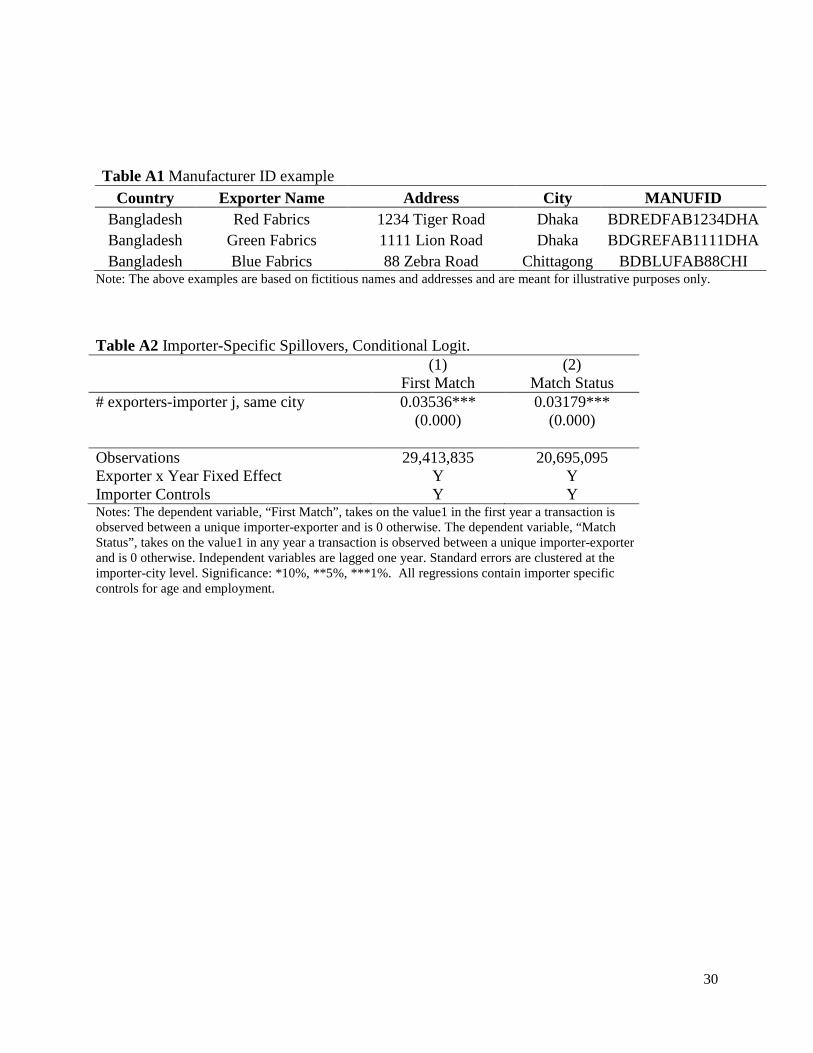
In order to compare our results to that in the existing literature, we implement a

conditional logit model as in Koenig et al (2010) with exporter-year fixed effects and time-

varying importer controls and report the results in Table A2. Koenig et al (2010) search for

destination-product specific spillovers on a French exporter’s decision to start exporting.

Implementing a conditional logit model with year and firm-product-country fixed effects, they

find that an additional exporter in the neighborhood increases the likelihood of exporting to the

same destination within a product category by 1.07 percentage points.

Our conditional logit estimation results imply that an additional exporter in the

neighborhood increases the likelihood of exporting to the same buyer for the first time by 0.70

percentage points and overall by 0.80 percentage points.21 Positing that the decision to export to

a country is comprised of the total sum of the decisions to export to a buyer within the country,

we can reasonably argue that destination-specific spillovers, estimated in the existing literature,

subsume importer-specific spillovers. Following this line of reasoning, the above results suggest

that importer-specific spillovers account for about 65% (75%) of destination-specific spillovers

for first time (ongoing) trade pair relationships. This is economically significant and indicates the

importance of isolating export spillovers that are buyer-specific.

4.2 Heterogeneous spillover effects

In Tables 4 and 5, we estimate equations (2.7) and (2.8) separately for small, medium,

and large exporters. Exporters are designated into three size categories based on their average

export sales in each year – large exporters have sales in the first quantile, medium exporters have 21 Marginal effects are calculated using the “margins” command in STATA.

17

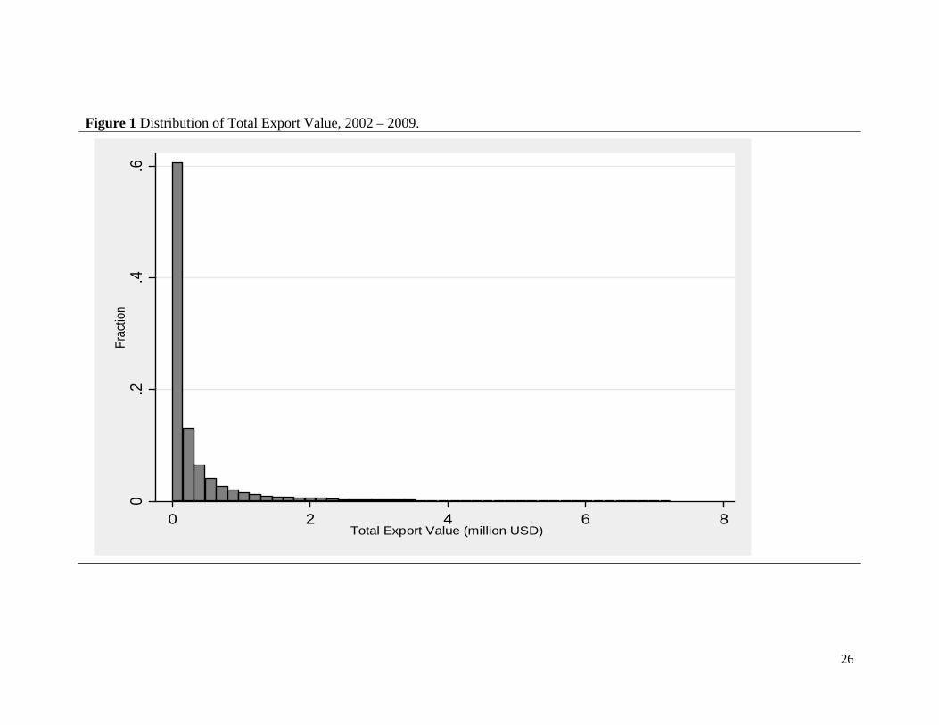
sales in the second quantile, and small exporters have sales in the third quantile. Figure 1 shows

the distribution of export value over our sample period. We see that about three-quarters of

annual Bangladeshi textile export transactions are valued at less than $500,000.

In addition to establishing the heterogeneity of the spillover effects based on exporter

characteristics, this exercise addresses and alleviates concerns about results predominantly being

driven by the presence of multi-plant firms. The concern about multi-plant firms is that although

our spillover variable correctly assigns manufacturers to the cities they are located in, it is

possible that the headquarter, rather than the manufacturing location of a multi-plant firm, is the

unit responsible for developing and maintaining trade relationships. Since we do not have firm

level information for the Bangladeshi manufacturers in our sample, we offer two reasons why we

believe our results are not disproportionately being driven by the presence of multi-plant firms.

First, the export-oriented Bangladeshi textile sector is characterized by a large number of

small firms rather than a few large firms that are also likely to have multiple plants (Yamagata,

2007). Second, we re-run our regressions on three separate samples that are divided according to

exporters’ average sales. It is reasonable to assume that manufacturing units of multi-plant firms

will tend to be larger in terms of total export value and therefore if the presence of such exporters

in our sample are disproportionately driving our results we would expect the spillovers to be

more pronounced for large exporters. However, we find the opposite result – spillovers are

strongest for small exporters. Intuitively, this makes sense because we would expect smaller

exporters to benefit more from the presence of neighboring exporters selling to the same buyer

since large exporters are more likely to have well-established, internal networks that facilitate

fostering and maintaining buyer-seller relationships.

18

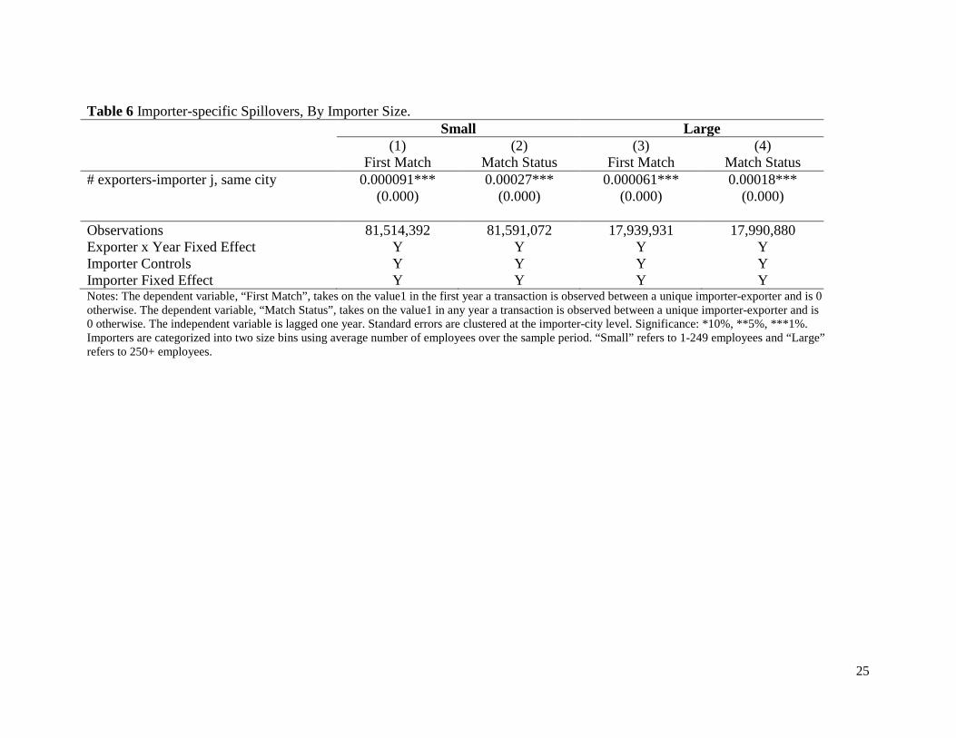
In Table 6, we estimate equations (2.7) and (2.8) separately for small and large U.S.

importers. This is motivated by evidence that there is substantial heterogeneity within U.S.

trading firms in terms of size and this could mask interesting patterns in the spillover variable of

interest as discussed below. Bernard, Jensen, and Schott (2010) document that pure wholesalers

and retailers (defined as importers with 100% of their employment in either of those two sectors)

are smaller in terms of employment, trade value and domestic sales, operate fewer U.S.

establishments and are present in fewer U.S. states. Meanwhile “mixed” firms (defined as firms

with less than 100% employment in retailing and/or wholesaling) are substantially larger, trade

more products, trade with more countries, and are more likely to engage in related-party trade. In

our sample, more than half of U.S. importers are wholesalers while a third are manufacturing and

retail firms.

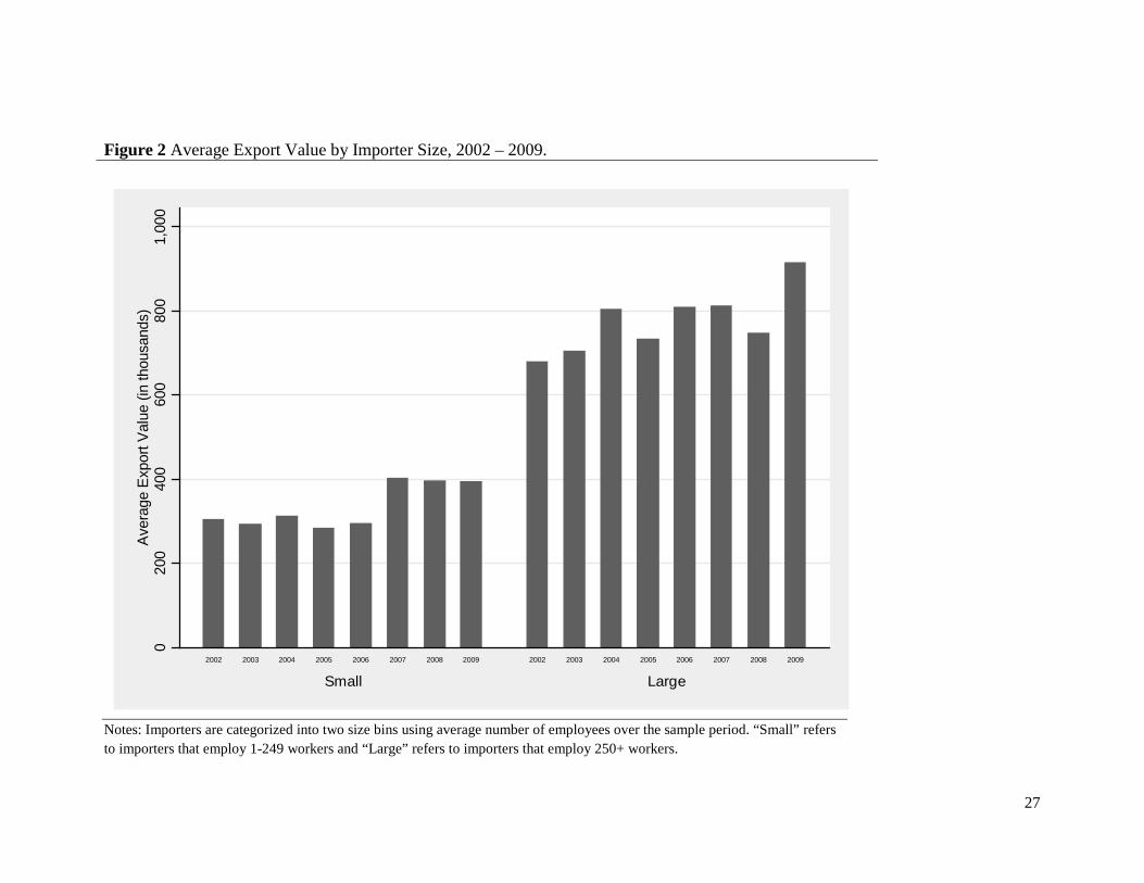
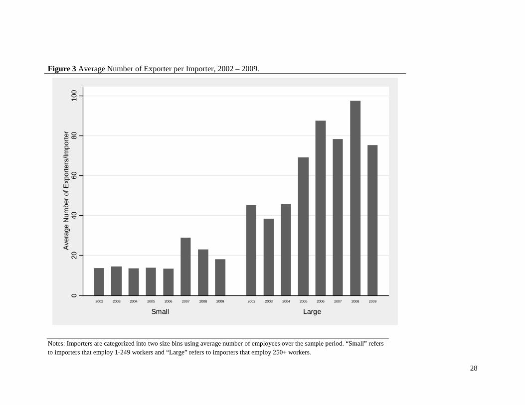
Figures 2 and 3 show that the average export value and number of exporters per importer

differ vastly by importer size in each of the sample years. The average import value of small

importers are less than half that of large importers. Large importers also transact with almost

double the number of Bangladeshi exporters compared to small importers, on average. Large

firms in the U.S. importing textiles from Bangladesh are likely to behave differently in procuring

suppliers and trading with them and so we expect spillover effects to differ across size

categories. For instance, small U.S. importers might be more reliant on their existing suppliers

for information on potential future suppliers than large U.S. wholesalers and retailers, who might

have alternative means of search. Similarly, on the Bangladeshi side, exporters might find it

more difficult to search and match with smaller U.S. buyers.

Indeed, we do find support for the hypothesis that spillovers play a larger role in buyer-

seller matches when the buyer is small. The results are presented in Table 6. We divide the

19

sample by importer size – small and large. Columns (1) and (2) present results for the sample of

small importers and columns (3) and (4) for the sample of large importers. Looking at columns

(1) and (3) where the dependent variable is the probability of a first match, we find that spillover

effects for large firms are smaller than that for small firms, though both effects are positive and

statistically significant. Results in columns (2) and (4), where the dependent variable is the

match status between pairs in general, exhibit a similar pattern. The spillover effects are larger

when the Bangladeshi textile manufacturer exports to a small U.S. importer.

5. Conclusion

This paper finds a statistically positive and economically significant role for spillovers

that are specific to the buyer in the decision to begin and continue trade relationships between an

exporter and importer, thus, building on the existing empirical body of evidence that finds

evidence for export spillovers that are specific to destinations and products. It also adds to the

nascent investigations on matches between buyers and sellers in both the international trade and

urban agglomeration economies literatures. Specifically, we investigate if the presence of other

exporters in the neighborhood of a firm, selling to a particular foreign buyer, facilitates a match

between the firm and this buyer.

Our results suggest that a one percent increase in the number of exporters in a city selling

to a buyer results in a 0.19% (0.34%) increase in the likelihood of a match with the same buyer

for the first time (ongoing). Comparison with existing evidence suggests that this effect is

economically significant – importer-specific spillovers account for about three-quarters of

destination-product specific spillovers. We also document evidence of positive importer-specific

export spillovers that vary with both exporter and importer characteristics. In particular,

20

spillovers are stronger for small exporters and small importers. Together, these results establish

the importance of isolating the buyer-specific component of export spillovers and recognizing

that there may be further variation in spillovers depending on exporter and importer

characteristics, namely size. Our study underscores the importance of linking firm-trade

transactions data between country pairs to shed further light on the determinants of buyer-seller

relationships.

21

References

Bernard, A. B., Jensen, J. B., 2004. Why some firms export? Review of Economics and Statistics 86(2), 561-569. Bernard, A. B., Jensen, J. B. Schott, P. K., 2010. Wholesalers and retailers in U.S. trade. American Economic Review Papers and Proceedings 408-413. Duranton, G., Puga, D., 2004. Micro-Foundations of Urban Agglomeration Economies, in V. Henderson and J.-F. Thisse (eds.), Handbook of Regional and Urban Economics, Vol. 4. Amsterdam: North-Holland, pp. 2063–2117. Eaton, J., Eslava, M., Jinkins, D., Krizan, C.J., Tybout, J., 2013. A search and learning model of export dynamics. mimeo. Jarmin, R. S., Miranda, J., 2002. The longitudinal business database. Working paper 02-17, Center for Economic Studies, U.S. Census Bureau. Koenig, P., 2009. Agglomeration and the export decisions of French firms. Journal of Urban Economics 66, 186-195. Koenig, P., Mayneris, F., Poncet, S., 2010. Local export spillovers in France. European Economic Review 54, 622-641. Monarch, R., 2013. “It’s not you, it’s me”: Breakups in U.S.-China trade relationships. mimeo. Puga, D., 2010. The magnitude and causes of agglomeration economies. Journal of Regional Science 50(1), 203-219. Trade Policy Review, 2012. World Trade Organization, WT/TPR/G/270. Yamagata, T., 2007. Prospects for development of the garment industry in developing countries: What has happened since the MFA phase-out? IDE Discussion Paper No. 101.

22

Table 1 Summary Statistics. All Importers Small Importers Large Importers Mean Std. Dev. Mean Std. Dev. Mean Std. Dev. Number of HS-10 products/pair 8.45 9.67 7.13 8.645 9.875 10.89

Export value/pair (in thousands) 524 1,552 342 945 784 2,111

Number of exporters/importer 39.10 60.77 17.97 31.45 71.47 76.84

Number of Exporters-Importer , Same City 0.53 3.20 0.37 1.81 1.42 6.85 Notes: The statistics are based on the sample of U.S. import transactions with Bangladesh in textile products only between 2002 and 2009; “Pair” refers to a unique importer-exporter combination; Export values are in nominal U.S. dollars and rounded to the nearest integer. “Small” refers to importers that employ 1-249 workers and “Large” refers to importers that employ 250+ workers.

23

Table 2 First Match, Importer-Specific Spillovers. (1) (2) (2) First Match First Match First Match # exporters-importer j, same city 0.00013*** 0.00013*** 0.000069*** (0.000) (0.000) (0.000) Observations 131,965,095 99,454,323 99,454,323 Year Fixed Effect Y - - Exporter x Year Fixed Effect - Y Y Importer Controls - Y Y Importer Fixed Effect - - Y Notes: The dependent variable, “First Match”, takes on the value1 in the first year a transaction is observed between a unique importer-exporter and is 0 otherwise. The independent variable is lagged one year. Standard errors are clustered at the importer-city level. Significance: *10%, **5%, ***1%.

Table 3 Match Status, Importer-Specific Spillovers. (1) (2) (3) Match Status Match Status Match Status # exporters-importer j, same city 0.00030*** 0.00030*** 0.00021*** (0.000) (0.000) (0.000) Observations 132,119,512 99,581,952 99,581,952 Year Fixed Effect Y - - Exporter x Year Fixed Effect - Y Y Importer Controls - Y Y Importer Fixed Effect - - Y Notes: The dependent variable, “Match Status”, takes on the value1 in any year a transaction is observed between a unique importer-exporter and is 0 otherwise. The independent variable is lagged one year. Standard errors are clustered at the importer-city level. Significance: *10%, **5%, ***1%.

24

Table 4 First Match, By Exporter Size. Large Medium Small First Match First Match First Match # exporters-importer j, same city 0.00005*** 0.00004*** 0.00012*** (0.000) (0.000) (0.000) Observations 32,004,507 31,985,128 31,927,890 Exporter x Year Fixed Effect Y Y Y Importer Controls Y Y Y Importer Fixed Effect Y Y Y Notes: The dependent variable, “First Match”, takes on the value1 in the first year a transaction is observed between a unique importer-exporter and is 0 otherwise. The independent variable is lagged one year. Standard errors are clustered at the importer-city level. Significance: *10%, **5%, ***1%. Exporters are designated as small, medium, large based on three size quantiles using average value of export sales each year in the sample period.

Table 5 Match Status, By Exporter Size. Large Medium Small Match Status Match Status Match Status # exporters-importer j, same city 0.00009*** 0.00007*** 0.00047*** (0.000) (0.000) (0.000) Observations 32,022,528 32,010,240 32,010,240 Exporter x Year Fixed Effect Y Y Y Importer Controls Y Y Y Importer Fixed Effect Y Y Y Notes: The dependent variable, “Match Status”, takes on the value1 in any year a transaction is observed between a unique importer-exporter and is 0 otherwise. The independent variable is lagged one year. Standard errors are clustered at the importer-city level. Significance: *10%, **5%, ***1%. Exporters are designated as small, medium, large based on three size quantiles using average value of export sales each year in the sample period.

25

Table 6 Importer-specific Spillovers, By Importer Size. Small Large (1) (2) (3) (4) First Match Match Status First Match Match Status # exporters-importer j, same city 0.000091*** 0.00027*** 0.000061*** 0.00018*** (0.000) (0.000) (0.000) (0.000) Observations 81,514,392 81,591,072 17,939,931 17,990,880 Exporter x Year Fixed Effect Y Y Y Y Importer Controls Y Y Y Y Importer Fixed Effect Y Y Y Y Notes: The dependent variable, “First Match”, takes on the value1 in the first year a transaction is observed between a unique importer-exporter and is 0 otherwise. The dependent variable, “Match Status”, takes on the value1 in any year a transaction is observed between a unique importer-exporter and is 0 otherwise. The independent variable is lagged one year. Standard errors are clustered at the importer-city level. Significance: *10%, **5%, ***1%. Importers are categorized into two size bins using average number of employees over the sample period. “Small” refers to 1-249 employees and “Large” refers to 250+ employees.

26

Figure 1 Distribution of Total Export Value, 2002 – 2009. 0

.2.4

.6Fr

actio

n

0 2 4 6 8Total Export Value (million USD)

27

Figure 2 Average Export Value by Importer Size, 2002 – 2009.

020

040

060

080

01,

000

Aver

age

Expo

rt Va

lue

(in th

ousa

nds)

Small Large2002 2003 2004 2005 2006 2007 2008 2009 2002 2003 2004 2005 2006 2007 2008 2009

Notes: Importers are categorized into two size bins using average number of employees over the sample period. “Small” refers to importers that employ 1-249 workers and “Large” refers to importers that employ 250+ workers.

28

Figure 3 Average Number of Exporter per Importer, 2002 – 2009. 0

2040

6080

100

Ave

rage

Num

ber o

f Exp

orte

rs/Im

porte

r

Small Large2002 2003 2004 2005 2006 2007 2008 2009 2002 2003 2004 2005 2006 2007 2008 2009

Notes: Importers are categorized into two size bins using average number of employees over the sample period. “Small” refers to importers that employ 1-249 workers and “Large” refers to importers that employ 250+ workers.

29

APPENDIX

Figure A1 Administrative Unit Map, Bangladesh

Source: http://www.fao.org/fileadmin/templates/faobd/img/Administrative_Unit_Map.jpg

30

Table A1 Manufacturer ID example Country Exporter Name Address City MANUFID

Bangladesh Red Fabrics 1234 Tiger Road Dhaka BDREDFAB1234DHA Bangladesh Green Fabrics 1111 Lion Road Dhaka BDGREFAB1111DHA Bangladesh Blue Fabrics 88 Zebra Road Chittagong BDBLUFAB88CHI

Note: The above examples are based on fictitious names and addresses and are meant for illustrative purposes only.

Table A2 Importer-Specific Spillovers, Conditional Logit. (1) (2) First Match Match Status # exporters-importer j, same city 0.03536***

(0.000) 0.03179***

(0.000) Observations 29,413,835 20,695,095 Exporter x Year Fixed Effect Y Y Importer Controls Y Y Notes: The dependent variable, “First Match”, takes on the value1 in the first year a transaction is observed between a unique importer-exporter and is 0 otherwise. The dependent variable, “Match Status”, takes on the value1 in any year a transaction is observed between a unique importer-exporter and is 0 otherwise. Independent variables are lagged one year. Standard errors are clustered at the importer-city level. Significance: *10%, **5%, ***1%. All regressions contain importer specific controls for age and employment.