Business CyclesBusiness Cyclesyy.... in data.... in data

All data within are from the Bureau of Economic Analysis, unless otherwise indicated.

© 2011-2014 Gary R. Evans. May be used only for non-profit educational purposes without permission of the author. All other uses are prohibited.

Topical issue: the rapid devaluation of Topical issue: the rapid devaluation of emerging market currencies in 2014emerging market currencies in 2014

What is a business cycle?What is a business cycle?The business cycle is an economic phenomenon measured by, in terms of the real GDP growth rate, the movement from a peak to a trough (recession) back to a peak (expansion). A recession is loosely defined to be two or more consecutive quarters when the real GDP growth rate is negative.

Business cycles are investigated by a private research organization calledBusiness cycles are investigated by a private research organization called The National Bureau of Economic Research (see http://www.nber.org). The NBER has a more subtle definition of recessions:

"A i i i ifi d li i i i i d h"A recession is a significant decline in economic activity spread across the economy, lasting more than a few months, normally visible in real GDP, real income, employment, industrial production, and wholesale-retail sales. A recession begins just after the economy reaches a peak of activity andA recession begins just after the economy reaches a peak of activity and ends as the economy reaches its trough. Between trough and peak, the economy is in an expansion."

For a detailed explanation of how the NBER determines the turning points of cycles, seehttp://www.nber.org/cycles/recessions.html

Post WWII business cyclesPost WWII business cycles

Contraction: Expansion:Duration in Months

Contraction: Expansion:Duration in Months

Peak Trough

Contraction: Peak to Trough

Expansion: Trough to Peak (pre)

April 1960-2 February 1961-1 10Peak Trough

Contraction: Peak to Trough

Expansion: Trough to Peak (pre)

April 1960-2 February 1961-1 10p yDecember 1969-4 November 1970-4 11 106November 1973-4 March 1975-1 16 36January 1980-1 July 1980-3 6 58

p yDecember 1969-4 November 1970-4 11 106November 1973-4 March 1975-1 16 36January 1980-1 July 1980-3 6 58July 1981-3 November 1982-4 16 12July 1990-3 March 1991-1 8 92March 2001-1 November 2001-4 8 120

July 1981-3 November 1982-4 16 12July 1990-3 March 1991-1 8 92March 2001-1 November 2001-4 8 120

Note the relative duration of contractions relative to expansions.

December 2007-4 June 2009-2 18 73December 2007-4 June 2009-2 18 73

Note the relative duration of contractions relative to expansions.Source: National Bureau of Economic Research, current to February 1, 2014

Historical average of all cyclesHistorical average of all cyclesg yg y

Duration in MonthsDuration in Months

Average all cycles:

Contraction: Peak to Trough

Expansion: Trough to

PeakAverage all cycles:

Contraction: Peak to Trough

Expansion: Trough to

PeakAverage, all cycles: Trough Peak1854-1919 (16 cycles) 22 271919-1945 (6 cycles) 18 351945 2009 (11 l ) 11 58

Average, all cycles: Trough Peak1854-1919 (16 cycles) 22 271919-1945 (6 cycles) 18 351945 2009 (11 l ) 11 58

Note how much milder business cycles have become in the

1945-2009 (11 cycles) 11 581945-2009 (11 cycles) 11 58

Note how much milder business cycles have become in the modern (post WWII) era.

Source: Same as previous slide. Data are current to February 1, 2014.

Real GDP Growth: Real GDP Growth: 19601960--201320138 How do the components compare?

Average:

4

6 3.13%

2

0

Green lines: BC troughs

4

-2

Simpler definition: Below 0.0% for 2 consecutive quarters is a recession.

BC troughs

-41960 1965 1970 1975 1980 1985 1990 1995 2000 2005 2010

Source: Bureau of Economic Analysis, National Income and Product Accounts, Table 1.1.

Consumption Consumption 19601960--20132013

15

20

10

0

5

-5

0

-101960 1965 1970 1975 1980 1985 1990 1995 2000 2005 2010

D bl d N d bl d S iDurable goods Nondurable goods Services

Note the relative volatility of durables and the stability of services.

Wh t d i ti ?Wh t d i ti ?What drives consumption?What drives consumption?(to be covered in more detail in theory section)(to be covered in more detail in theory section)

• Personal income• Access to creditAccess to credit• Interest rates (real estate and durables)

P i d l h• Perceived wealth– home equity– financial investments

• Expectations of the above

Investment Investment 19601960--20132013Compare this to consumption ranges!

40

50

Remember that

p g

20

30these are sensitive to interest rates.

0

10

20

-10

0

-30

-20

1960 1965 1970 1975 1980 1985 1990 1995 2000 2005 2010

Nonresidential RE Equipment Residential RE IP Products

Note the peaks and troughs (magnitude) of residential construction.

Government Purchases, Government Purchases, 19601960--20132013

8

10

12

4

6

8

0

2

-6

-4

-2

Why is this falling

-8

-6

1960 1965 1970 1975 1980 1985 1990 1995 2000 2005 2010

through here?

Federal State and local

"Automatic stabilizer?"

Elementary Macroeconomic AnalysisElementary Macroeconomic Analysisy yy y

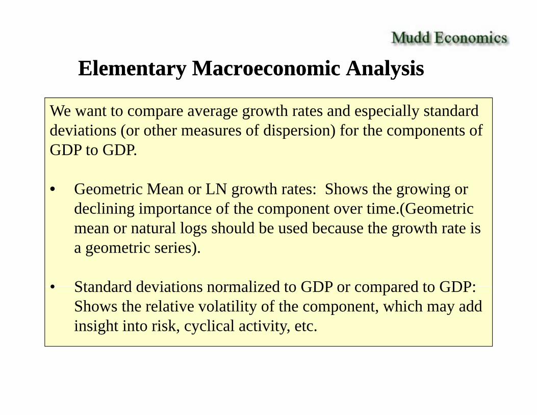
We want to compare average growth rates and especially standard deviations (or other measures of dispersion) for the components ofdeviations (or other measures of dispersion) for the components of GDP to GDP.

• Geometric Mean or LN growth rates: Shows the growing or declining importance of the component over time.(Geometric mean or natural logs should be used because the growth rate is g ga geometric series).

• Standard deviations normalized to GDP or compared to GDP:• Standard deviations normalized to GDP or compared to GDP: Shows the relative volatility of the component, which may add insight into risk, cyclical activity, etc.

A good proxy for cycle candidatesA good proxy for cycle candidatesA good proxy for cycle candidatesA good proxy for cycle candidatesWhen compared to GDP as a whole, if a component has a Real GDP geometric , pwider standard deviation it contributes to cycles, if smaller, it dampens cycles.

Real GDP geometric mean growth rate was 0.0304 1960-2010, smaller, it dampens cycles.geometric standard deviation is 0.0211

3.04%

Three alternative growth ratesDWBH: I am not going to ask you this!DWBH: I am not going to ask you this!

(point by point estimation from time-series data) Example from 1st 2 observations on left

Discrete: 0.15111

t

t

t

tt

XX

XXX

Geometric 1 15Working with raw time- tX 1

Discrete: 1.15raw timeseries data, we have to transform it

tX

Continuous(log): 0.13976to growth

rates, but which?

ttt

t XXX

X lnlnln 11

... calculating geometric mean and geometric ... calculating geometric mean and geometric DWBH: I am not going to ask you this!DWBH: I am not going to ask you this!

standard deviation standard deviation ((from from discretediscrete--converted data)converted data)

Geometric Mean value of Geometric standard deviation ofGeometric Mean value of growth rate:

Geometric standard deviation of the growth rate:

n n 1

gx ii

n n

x

1or

xi

n

1ln Typically used to calculate the mean and

gxne

ii1 dispersion of a log-normal distribution, here

we are stating that this must be used to the same for time-series data transformed to discrete rather than continuous growth rates

Remember – the growth rate will be expressed as 1.15 rather than 0.15.

discrete rather than continuous growth rates.

Real GDP component growth and standard Real GDP component growth and standard deviation , 1960deviation , 1960--2010 2010

Note: Very important slide to understand for exam.

How to interpret the previous slide ...How to interpret the previous slide ...GDP is an aggregate and all of the other categories are components of

the aggregate. Their weights vary from Services, which constitute 47% of GDP, to Residential Construction, which constitutes only 2.3%. The

l ili f GDP hi h h b d d d i i f i hvolatility of GDP, which we here represent by standard deviation of its growth rate, will obviously be impacted by the volatility of its components, which we represent by the individual standard deviations of their growth rates, derived from their variancesfrom their variances.

Generally, the higher the volatility of the component relative to the volatility of GDP, the more that component is raising the volatility of GDP. The net impact is also determined by the weight of the component The higherThe net impact is also determined by the weight of the component. The higher the weight, the more the impact. Maybe you can see it in the math.

(You are not accountable for the material below):

The sum of variances formula is below. In this context, the variance of GDP can be thought of as the extreme left term, and the individual Xs are the components. If the components are independent, the covariance term disappears. SD is the

i j jijii

ii

iii XXCovXVXV ,22

square root of Variance. Clearly the higher the weight, the higher the effect.

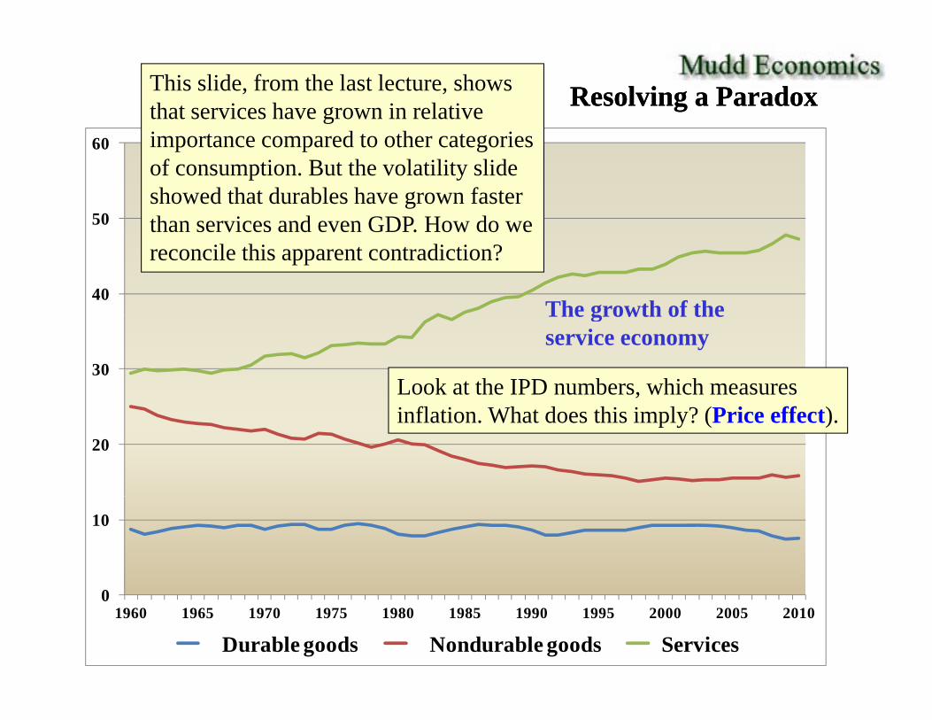
Resolving a ParadoxResolving a ParadoxThis slide, from the last lecture, shows that services have grown in relative i t d t th t i

50

60 importance compared to other categories of consumption. But the volatility slide showed that durables have grown faster than services and even GDP How do we

40

50

The growth of the

than services and even GDP. How do we reconcile this apparent contradiction?

30

The growth of the service economy

Look at the IPD numbers, which measures

20inflation. What does this imply? (Price effect).

10

01960 1965 1970 1975 1980 1985 1990 1995 2000 2005 2010

Durable goods Nondurable goods Services

Certain conclusions ...Certain conclusions ...• This has become a “service” economy

– and that has stabilized the cycle because the volatility f i d b l ti t d d d i tiof services, as measured by relative standard deviation,

is very low

• All classes of investment contribute to the cycleAll classes of investment contribute to the cycle• The two largest business cycle contributors are

typicallytypically– Durables (consumer)– Residential structures

• This is especially apparent when comparing component standard deviations to GDP (the aggregate)

Memo items ..Memo items ..

• Productivity gains are robust in services and durables– which combats inflationwhich combats inflation

• Importing manufactured goods also combats inflation unless the $$ is weakening

• The volatile categories are “interest sensitive”• Federal government purchases are not the same as

expendituresexpenditures– transfer payments are the difference

• Federal and state and local government purchases,Federal and state and local government purchases, especially the latter, do not necessarily counter-balance a recession.

Inflation and interest ratesInflation and interest ratesand the business cycle... and the business cycle

Source: All CPI numbers areSource: All CPI numbers are from The Bureau of Labor Statistics

Inflation: why a problem?Inflation: why a problem?

• Reallocates income and wealth unfairly– from lender to borrowerfrom lender to borrower– from salaried– from elderly (unless prepared)from elderly (unless prepared)– to speculators

• Injects tremendous uncertainty• Injects tremendous uncertainty– curbs investment

Inflation: Inflation: (continued)(continued)

• Seriously threatens financial marketsSeriously threatens financial markets– especially stocks

• Invites a policy response• Invites a policy response– the modern FRS crunch

A i fl i i• As goes inflation, so go interest rates

CPI Inflation Rate: CPI Inflation Rate: 19601960--20132013Average: 4%

14.00

16.00Annual % change

Double-digitAcceptable

10.00

12.00Double-digit hyperinflation

Acceptable level (about 2.5%)

G li

6.00

8.00Green lines: BC troughs

2.00

4.00

-2.00

0.00

1960 1965 1970 1975 1980 1985 1990 1995 2000 2005 2010

CPI for urban consumers, U.S. city average, all items,NSA. Source: Bureau of Labor Statistics

CPI and Mortgage and 10CPI and Mortgage and 10--year Treasury year Treasury

16

18

Bond Rates: Bond Rates: 19721972--20132013

12

14

16What story is found here?

As goes inflation, so will go mortgage rates and other

8

10

mortgage rates and other key rates.

4

6

0

2

-21972 1975 1978 1981 1984 1987 1990 1993 1996 1999 2002 2005 2008 2011

CPI 30 Yr FRM 10 Yr T-Bond

Source for interest rates: Federal Reserve Board data download program, H-15 series

Domestic NonDomestic Non--financial Debt / National Incomefinancial Debt / National Income

3.5

19621962--20122012

This is the total net indebtedness of all

3.0

This is the total net indebtedness of all parties in the U.S. economy (non-financial eliminates double counting) divided by National Income. This is a national proxy for

2.5our debt divided by our capacity to pay it.

Millennium i

2.0The 80s discover

dit

craziness

1.5

This is at the root of why we are in trouble.

Stabilitycredit

1.01962 1966 1970 1974 1978 1982 1986 1990 1994 1998 2002 2006 2010

Source (debt): Federal Reserve Flow of Funds Accounts, Z1 statistical release

© 2011-2014 Gary R. Evans. May be used for and only for non-profit educational purposes without permission of the author. All other uses are expressly prohibited.

Business Cycle MechanicsBusiness Cycle Mechanics... the pathology of the business cycle... the pathology of the business cycle

Sammy the ySeagull, consultant

The point here is to examine some general features of all business cycles.

... at the trough

Low interest ratesd i l• ... and a monetary stimulus

Pent up consumer demand• ... average auto age an example

Businesses lean and mean

... the expansion

Consumer-led (durables)Sometimes 5+% growth very earlySometimes 5+% growth very earlyReal estate often lagsP d i i i b i ll iProductivity gains can substantially increase

the time period and the rate of gain

... near the peakBottlenecks in s ppl ariseBottlenecks in supply ariseInflation/interest rates rising

d FRS li i• ... produces an FRS policy reactionRates of profit are squeezed

• ... which sometimes impacts the stock market• ... which can engender a negative “wealth

effect”effectSometimes speculative excess

Unemployment

... rises sharply during the recession... sometimes continues to rise into the

recovery

.. this is sometimes a long lag variable

Unemployment Unemployment RateRate19601960--2012, 2012, annual, % of civilian workforceannual, % of civilian workforce

12 Specifically, all wage earners above age 16, seasonally adjuisted.

8

10

Mean: 6.096.09%

6

8

4

Red represents the trough of business

2

Red represents the trough of business cycles. In recent cycles, unemployment lags the cycle by a few months.

01960 1965 1970 1975 1980 1985 1990 1995 2000 2005 2010

How this expansion, though, is not typicalHow this expansion, though, is not typical

Private employment is very slow to respond ...

From Caryn N Bruyere Guy L Podgornik and James R Spletzer “EmploymentFrom Caryn N. Bruyere, Guy L. Podgornik, and James R. Spletzer, Employment Dynamics Over the Last Decade, Monthly Labor Review Online, August 2011, Vol. 134, No. 8.

Why no bad recession in the earlyWhy no bad recession in the early 2000s?

• 1995-2000: Wealth effect of rising stock market

• 2000-2004: Wealth effect of rising home equityequity

• Easy monetary policy … record low interest ratesrates

• Generous fiscal policy … heavy tax cuts

Why a slow recovery now?Why a slow recovery now?y yy y• Bad mortgages/credit crisis still

hammering housinghammering housing.• Credit crisis spread past

financial sectorfinancial sector• Negative wealth effects of

declining home equity valuesdec g o e equ y v ues• Negative wealth effects of

declining stock and corporate g pbond markets

• Unemployment remains stubbornly high This graph is now old, but the

effect is still current ...

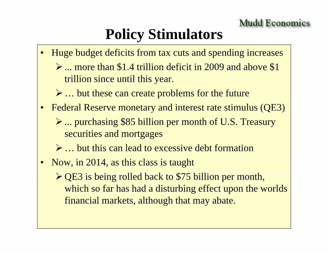
Policy Stimulators• Huge budget deficits from tax cuts and spending increases ... more than $1.4 trillion deficit in 2009 and above $1

trillion since until this yeartrillion since until this year.… but these can create problems for the future

• Federal Reserve monetary and interest rate stimulus (QE3)ede a ese ve o eta y a d te est ate st u us (Q 3) ... purchasing $85 billion per month of U.S. Treasury

securities and mortgages… but this can lead to excessive debt formation

• Now, in 2014, as this class is taughtQE3 i b i ll d b k t $75 billi thQE3 is being rolled back to $75 billion per month,

which so far has had a disturbing effect upon the worlds financial markets, although that may abate.