Business Cycle Accounting analysis of MonetaryPolicy Transmission in India

Kshitiz Mishra ∗ †

Shiv Nadar University

Date: November 25, 2019

This work is under progress. Please do not cite.

Abstract

We study the monetary policy transmission (MPT) or lack of it in Indian context using a BusinessCycle Accounting (BCA) framework. In the standard BCA setup we introduce a simple bankingsector motivated by Lahiri and Patel [9] where we capture MPT as transmission from change inTreasury bill rate to lending rates. We show using Bayesian MCMC methods that 1) MPT in Indiais weak, 2) labor wedges are responsible for up to 30% of the fluctuations in MPT, with share ofother real wedges varying from 17-25% and no role for nominal wedges. We then further augmentthe model to include a statutory liquidity ratio, and show that it does not affect transmission fromlending rate to real variables, and changes in SLR only affect the nominal interest rate.

1 Introduction

India adopted inflation targeting in the later half of 2016 with the intent to improve price andfiscal stability and reducing output and exchange rate volatility. In emerging market economies(EMEs) however there is considerable debate whether monetary policy transmission is adequate forenough for the central banks to be able to affect aggregate demand. Lahiri and Patel [9] note thatspecific institutional constraints, persistent shocks, legacy structures, multiple and conflicting policy

∗Corresponding Author. Email ID: kshitiz.mishra@snu.edu.in†This work was done under the supervision of Partha Chatterjee, Associate Professor, Shiv Nadar University.

1

objectives and poor financial integration can be a impeding factor in achieving monetary policygoals in EMEs.

Studies done on data prior to 2016 (Das [7], Mishra et al. [10]) look at the bank lending channel(from monetary policy to bank lending rates) and show that MPT in India is while in theoreticallyexpected direction, is incomplete. The latter paper also finds no evidence of changes in output andinflation from changes in monetary policy, and also finds no evidence of exchange rate channel beingimportant for the Indian economy. In recent work by Banerjee et al. [1], they use a DSGE frameworkto find that monetary transmission may not be weak if we use change in monetary base as indicatorof monetary policy, but is much weaker if we focus only on the policy rate as the instrument. In thispaper we attempt to use Business Cycle Accounting methodology developed by Chari et al. [6] tostudy MPT in the Indian economy.

Business Cycle Accounting models (BCA), introduced by [6] introduce multiple time varyingwedges in a stochastic optimal growth model, which capture deviations of the model from the data.There are four wedges in their model: efficiency, investment, labor and a government consumptionwedge, which account for the entire variation in output, hours worked, investment and consumption.Variations in these wedges capture propagation of primitive shocks through frictions and distortionsin a detailed structural macroeconomic model ([13]). Sustek builds a extended monetary businesscycle accounting model (MBCA), with a central bank where they include two additional nominalwedges: an asset market wedge and a Taylors rule wedge. They then apply the model to explainmovements in inflation and nominal interest rate.

Chari et al. [6] and Brinca et al. [3] show that detailed economies with primitive shocks andfrictions distorting the first order equilibrium conditions can be mapped via equivalence resultsinto the above defined wedges distorting the first order conditions in a BCA model (also referredas the prototype economy). The four real wedges distort the following equilibrium conditionsin the prototype economy respectively: the production function, the inter-temporal consumptioninvestment trade-off equation, the labor-leisure intra-temporal choice equation, and the aggregateresource constraint. Of the nominal wedges, the asset market wedge distorts the inter-temporalequation for bonds and the Taylors Rule wedge distorts the Taylors Rule followed by the Centralbank.

The business cycle accounting exercise has two components, first being the equivalence results,which are described in next section. Accounting of the business cycles makes up the secondcomponent, where we ascertain the role of each wedge in explaining macroeconomic fluctuationsvia a decomposition exercise. By definition of the model prototype economy, all wedges combined

2

should explain the entire variation in each of the observables, in the decomposition exercise westudy how the wedges impact each aggregate variable individually, by feeding in only one wedge ata time (and also feeding all but one wedge a time), generating simulated data of the observables andcomparing it to the actual series observed in the data.

The banking sector we introduce in the BCA setup is simple: the representative bank takesdeposits from household, uses those deposits to invest in government bonds or lends to firms. In thefirst model we dont have any frictions, thus MPT is perfect. In the second model we add a StatutoryLiquidity Ratio requirement, which makes MPT imperfect.

Our results point out to efficiency wedge as a prime factor in explaining fluctuations in outputupto 68%. These results are similar for to an earlier exercise where we estimated the MonetaryBusiness Cycle Accounting model for the Indian economy. Labor wedges in the first model areresponsible for accounting up to 30% of monetary policy transmission, while other real wedgesexplain it from 17-25%. Some of our preliminary results are in sync with Banerjee et al. [1], wherethey also find that TFP shocks explain up to 50% of output with no more than 20% contributionby monetary policy shocks. We do not however find any role for nominal wedges in accountingfor MPT. In the second model, similarly to Banerjee et al. [1] we dont find any impact of SLR onhindering MPT from nominal interest rate to lending rates. Also SLR does not affect transmissionfrom lending rates to output or hours worked. We also intend to expand the model to look at the rolenon-performing assets MPT in India.

2 Equivalence Results

Business Cycle Accounting models (or the prototype economy) are useful to understand businesscycle fluctuations because they nest several models of detailed economies, which thus providestheoretical foundations for each of the wedges. Efficiency wedge represents frictions at firm levelwhich cause inefficient allocation of inputs. Chari et al. [6] show that a prototype model withefficiency wedges is equivalent to a detailed economy with input-financing restrictions (say forsmaller firms), or a detailed economy with variable capital utilization. A prototype economy withonly labor wedge is similarly shown equivalent to a detailed economy with sticky wages.A prototype model with only investment wedge is shown to be equivalent to a detailed economy withfluctuations in investment specific technological change in Brinca et al. [3]. They also show thatcertain financial frictions like collateral constraints show up in a prototype economy as investmentwedge. Sustek [13] shows that a detailed economy with sticky prices is equivalent to labor and

3

capital wedges, where capital wedges imply a tax on capital unlike on investment as done theprototype BCA model. These authors however show that a tax (or wedge) on capital or investmentare same in theory and practice, at least in the case of US economy.Sustek also shows that bond and labor wedge in the prototype model are equivalent to a detailedeconomy with limited participation in asset markets with a variable working capital requirementssetup. Monetary policy wedge according to Sustek is equivalent to a economy with varying inflationtargets, which thus creates uncertainty in the implementation of a dedicated monetary policy rule bythe central bank.

3 The Model

In this section we describe the BCA model augmented with a simple banking sector. It is aneoclassical growth model which consists of a) a representative household, b) a representative firm,c) government and a representative bank, with 6 exogenous wedges. The household maximizes itslifetime utility by maximizing consumption, leisure and investment. The firm maximizes profits byselecting optimal labor and capital in each time period. The government collects distortionary taxesin order to finance its exogenous expenditure. The bank invests in government securities and alsoloans to firms, and collects deposits from households and also pays a return on those deposits. Thewedges are efficiency wedge 0C , investment wedge 1/(1 + gGC), labor wedge (1 − g;C), governmentwedge 6C , deposit wedge 1/(1 + g3C) and Taylor’s Rule wedge 'C . We add an extra wedge in the SLRmodel.

Note that we have replaced the bond wedge in the standard Monetary Business Cycle Accountingmodel Sustek [13] with a deposit wedge, however they both are equivalent, except here the householddeposits savings in bank which then invests in Treasury bills and lends to firms.

3.1 Model Description (with Perfect Monetary Policy transmission)

The representative household maximizes expected lifetime utility by optimizing consumption 2C ,labor ;C , investment GC and nominal deposits �C in banks:

max{2C ,GC ,;C ,1C ,�C }

�C

∞∑C=0

VC* (2C , 1 − ;C) (1)

where* (2, 1 − ;) = (2(1 − ;)k) (1−f))/(1 − f) (2)

4

s.t.2C + (1 + gGC)GC + (1 + g3C) (

�C

?C (1 + 83C )− �C−1

?C) = AC:C + (1 − g;C)FC ;C + CAC (3)

where 83 is the interest rate paid by the banks on deposits by households. and the capital accumulationequation

(1 + WI) (1 + W0):C+1 = (1 − X):C + GC − q(GC

:C) (4)

where GC is the investment, CAC is the government transfer, FC is the wage rate, AC is the rental rate oncapital, V is the subjective discount factor, :C is the capital stock, X is the depreciation rate, (1 + WI)is the growth rate of population and (1 + W0) is the growth rate of labor augmenting technology.q(.) is the investment adjustment cost given by common specification:

q( G:) = 0

2( G:− 1)2 (5)

where b = (1 + W0) (1 + WI) − 1 + X. The representative firm solves the following problem:

max{:C ,;C }

� (:C , 0C ;C) − AC:C − FC ;C (1 + F28 5C ) (6)

where 8 5 is the lending rate from banks to firms, and

� (:, 0;) = :\ (0(1 − ;))1−\ (7)

The central bank manages the nominal interest rate on bonds via the following rule:

'C = (1 − dA) [' + lH (ln HC − ln H) + lc (cC − c)] + dA'C−1 + 'C (8)

where dA ∈ [0, 1], and cC = ln ?C − ln ?C−1, where p is the price level.The government sets taxes (g;C and gGC) and transfers each period to satisfy its budget constraint:

6C + CAC = g;CFC ;C + gGCGC (9)

Banks take deposits as given, and choose loans !C and government bonds /C by solving thefollowing problem:

max!C ,/C

�C

∞∑C=0(1 + 8 5

C−1)!C−1 + (1 + 'C−1)/C−1 + (1 + 83C−1)�C−1 + �C − /C − !C (10)

subject to the following constraints:

�C = /C + !C + "C (11)

where "C are the mandated amount of reserves (as a fraction XA of deposits) with the Central bank,at return at 8A .

The variables y, x, c, k, w, tr are in de-trended per-capita terms (say with a aggregate variable +C ,EC =

+C#C (1+WC0)

, where #C is the population at time t).

5

3.2 Model Description (with Statutory Liquidity Ratio)

In the augmented model with a exogenous SLR requirement imposed by the government, weneed to change the banking problem slightly:

max!C ,/C

�C

∞∑C=0(1 + 8 5

C−1)!C−1 + (1 + 'C−1)/C−1 + (1 + 83C−1)�C−1 + �C − /C − !C (12)

subject to the following constraints:

�C = /C + !C + "C (13)

and/C = U�C (14)

where U is the statutory liquidity ratio.Now since we have only one identifying equation for 8 5C and 'C , we define a additional wedge

�C = 'C − 8 5C . This is a wedge because if the transmission was perfect as in the first model, then �Cwould always equal zero.

3.3 Solving the Model

F.O.C. with respect to �C :−_C?C+ _C+1?C+1

Vℎ (1 + 83C ) = 0 (15)

From consumption F.O.C. we know that

*′2C= _C = 2C

−f (1 − ;C)k(1−f) (16)

substituting which into the above equation gives us:2C−f (1 − ;C)k(1−f) ?C+1

?C+ ˆ2C+1−f (1 − ;C+1)k(1−f)

?C+1V(1 + 83C ) = 0 (17)

Solving Bank’s optimization problem with respect to !C and 'C we get two equations:

83C = (1 − X)'C + X8A (18)

and85C = 'C (19)

Substituting the second in first equation we get 83C = 85C − X'C + X8A . We define LR Diff = 8

5C − X'C as

our key variable to capture monetary policy transmission.In the second model with a SLR requirement, our FOC is

83C = U'C + (1 − U − XA)8 5C + XA8A (20)

6

From equations (19) and (20) in perfect MPT case and the case with SLR resp., we can seewhy having a mandatory SLR requirement can reduce monetary policy transmission. In the firstequation changes in nominal interest rate are transmitted immediately to deposit rate and lendingrates (one-to-one), but in case of SLR, for every rupee of deposits, the bank has to invest a fractionXA in government securities, and then the leftover amount can be used for lending to firms. Thus ifnominal interest rate changes, it is possible that only deposit or lending rate may change [9].

3.4 Equilibrium Analysis

The four real wedges are thus defined in such a away that an increase in them leads to a increase inoutput (Chakraborty and Otsu [4]). If efficiency wedge 0C increases, production efficiency increases.If labor wedge (1 − g;C) increases, it leads to higher returns from labor for the representativehousehold, thus incentivizing a greater supply of labor leading to higher output. Similarly, withinvestment wedge 1/(1 + gGC), a higher value of the investment wedge increases investment, thusincreasing production, and a similar argument holds for the deposit wedge 1/(1+g3C). An increase ingovernment wedge also increases total output via increasing aggregate demand, but also crowds outconsumption and investment via increasing interest rates, so it cant be considered as a ’improvement’.

An increase in 'C cannot be construed as an improvement either, as it represents shocks to theTaylor’s rule, representing frictions in the central bank’s design and implementation of the Taylor’smonetary policy rule. Tien et al. [14] call shocks to Taylors rule as the shocks that cause a differencebetween a targeted federal funds rate based on Taylors rule with perfect foresight and a Taylors rulewith federal funds rate actually set by using forecasts of output and inflation.

The Competitive Equilibrium is thus defined as a sequence of prices [AC , FC , 'C , ?C]∞C=0, andquantities [HC , 2C , GC , 1C , 6C , ;C , :C+1, CAC]∞C=0 and 6 exogenous wedges efficiency wedge 0C , investmentwedge 1/(1 + gGC), labor wedge (1 − g;C), government wedge 6C , deposit wedge 1/(1 + g3C), andTaylor’s rule wedge 'C such that:

1. The household maximizes its expected lifetime utility assuming[AC , FC , ?C , g;C , gGC , g1C]∞C=0 and the initial value of capital :0 as given;

2. The firm maximizes its profit every time period assuming [AC , FC , 0C]∞C=0 to be given;3. Capital and labor markets clear every time period;4. Central bank sets the nominal interest rate on bonds in accordance with the Taylor’s rule;5. The resource and government budget constraint hold every time period;6. The stochastic process BC = (ln 0C , g;C , gGC , ln 6C , g1C , 'C)′ follows the VAR(1) process: BC+1 =

%0 + %BC + &nB,C+1, n ∼ # (0, +) where n follows a standard normal distribution with mean

7

zero and positive-semidefinite variance-covariance matrix V. %0 is a 6x1 column vector, P is a6x6 transition matrix. We thus have total of 63 parameters to estimate.

Note that this is the description for a competitive equilibrium for theModel with perfect Monetarypolicy transmission. In the case with SLR, we have seven wedges, hence the modified stochasticprocess will be BC = (ln 0C , g;C , gGC , ln 6C , g1C , 'C , �C)′, and we need to estimate 84 parameters.

The first order conditions that characterize the competitive equilibrium (besides Taylors Rule)are as follows:

2C + 6C + (1 + W0) (1 + WI) ˆ:C+1 − (1 − X) :C = HC = :C\ (0C ;C)\−1 (21)

k2C (1 + F2 (8 5C − 1))1 − ;C

= (1 − g;C) (1 − \) :C ;−\C I1−\C (22)

The labor FOC is the same as in the standard BCA model except the working capital term.

(1 + gGC)2C−f (1− ;C)k(1−f) = V�C ˆ2C+1−f (1− ;C+1)k(1−f) [\ ˆ:C+1\−1(0C+1;C+1)1−\ + (1− X) (1 + gGC+1)]

(23)

(1 + g3C)?C (1 + 'C)

2C−f (1 − ;C)k(1−f) = V�C ˆ2C+1−f (1 − ;C+1)k(1−f)

(1 + g3C+1)?C+1

(24)

The efficiency wedge is thus equivalent to a labor-augmenting technical shock. The labor wedgedraws a friction in the intra-temporal marginal rate of substitution between the marginal product ofconsumption and labor. The investment wedge (bond wedge) draws a friction in the Euler equationfor capital (bonds), between the inter-temporal marginal rate of substitution between marginalproduct of consumption today against the marginal product of investment (bond holdings) in thenext time period.

3.5 Data

We apply the Business Cycle Accounting procedure to Indian quarterly data from 1996.Q1-2017.Q4. The source of data is RBI Quarterly National Accounts, with base year 2011-12. Hoursworked are calculated by assuming 14 working hours in a day, multiplied by number of daysfactories worked in each year (data from Annual Survey of Industries). Capital stock is calculated

8

via perpetual inventory method, using the investment data and assuming a initial value of capitalstock (Chari et al. [5]). Data on lending rates is from SBI Prime Lending Rate.

Figure 1 shows the deseasonalized macroeconomic aggregates.

3.6 Empirical Methodology

We first calibrate parameter values based on the data and existing literature. In the second stepwe solve the log-linearized model using the Gensys method by (Sims [12]) and then estimate thelinearized decision rules for the wedges using Bayesian MCMC methods (Herbst and Schorfheide[8]). In the last step, we explain the role of wedges in business cycle fluctuations by carrying out thedecomposition exercise: we hold all but one wedge constant to isolate the marginal impact of thatwedge on observables.

3.6.1 Calibration

We borrow the CKM values for the following parameters: (quarterly) subjective discount rate,time allocation parameter k and capital share. WI is the growth rate of population calculated fromthe data. W0 is the growth rate of labor augmenting technology (labor productivity) calculated fromthe data such that the detrended log output has a zero mean. b is the adjustment cost parameter setequal to W0 + WI + X, and the adjustment cost parameter a is calculated such that the elasticity, [ ofthe price of capital with respect to the investment-capital ratio is 0.25. At the steady state, [ = ab, soknowing [ and b can allow us to calculate a.

Table 1 lists the parameter values.

3.6.2 Solution and Estimation of the Model

We solve the log-linearized model using Gensys (Brinca et al. [2]), and then estimate it using alinearized state space model:

-C+1 = �-C + �nC+1 (25)

.C = �-C + lC (26)

9

Table 1: Parameters

Parameter Description Value

X Depreciation rate 10%

W0 Growth rate of labor productivity .0138

WI Growth rate of population .0037

k Leisure Preference 2.5

\ Capital share 1/3

V Subjective discount rate .99

XA Fraction of Deposits as Reserves 5%

8A Interest rate on Reserves 1%

F2 Working Capital 0.5

lC = �lC−1 + [C (27)

where

-C = [;>6(:C), ;>6(0C), g;C , gGC , ;>6(6C), g3C , 'C , 1]′

and.C = [;>6(HC), ;>6(GC), ;>6(;C), ;>6(6C), 8 5C − XA'C , cC]

and matrices A and B are calculated from Gensys.We estimate the variable 8 5C − XA'C because with perfect monetary policy transmission, it should

equal 83C − XA8A . Since this equality does not hold in data, the discrepancies will be captured in thewedges.

Our aim here is to estimate the stochastic process BC for the wedges

BC+1 = %0 + %BC +&nB,C+1, n ∼ # (0, +)

whereBC = (;>6(0C), g;C , gGC , ;>6(6C), g3C , 'C)

and n is i.i.d. and follows standard normal distribution with mean zero and variance-covariancematrix V.

In the second model with a SLR requirement, -C and .C are changed as follows:

-C = [;>6(:C), ;>6(0C), g;C , gGC , ;>6(6C), g3C , 'C , �C , 1]′

10

and.C = [;>6(HC), ;>6(GC), ;>6(;C), ;>6(6C), 'C , cC , 8 5C ]

It is important to note that estimating this stochastic process is necessary only because of theinvestment and deposit wedges. The efficiency wedge can be directly calculated using the firm’s FOC.The labor wedge similarly can be calculated from the households FOC. The government wedge is justthe government expenditure plus net exports taken directly from the data. Estimating investment/bondwedge is necessary because in equations (23) and (24), the RHS contains expectations over thefuture values of capital stock, consumption and wedges.

We estimate the model using Bayesian RWMH-MCMC method 1. The reason why we usedBayesian methods is because our data is considerably short: we have 88 observations to estimate 63parameters (6 in %0, 36 in P and 21 in V). When applying Bayesian methods, the prior informationspecified acts as extra information, and thus Bayesian methods are useful in cases of low samplesize. The estimated scale potential reduction factor was 1.07.

The priors for %0, P and Q matrices are given in Table 2.For the SLR case with 84 parameters (7 in %0, 49 in P and 27 in V), the priors are in Table 3.

4 Results

We plot the normalized (by base year values) output and wedges in Figure 2 for the Perfect MPTcase, and Figure 3 and Figure 4 for SLR=0.15 and 0.25 resp. (note that the output and the wedgesare de-trended).

First thing we see is that output and efficiency wedges follow each other very closely. A fall inefficiency wedge directly implies below trend growth in labor productivity. In our data we face threesuch major declines, first around 1999-02, then 2008-09, and lastly during 2011-12. All these threeperiods correspond to recessions in India ([11]).

We also see that labor wedges seem to follow a pattern opposite to output from 1999-2008,suggesting some improvements in labor wedge (reductions in labor market frictions), and but thenfall consistently from 2008 onwards. Investment wedges however seem to rise, and from 2004-2001seem to be associated with rise seen in output. Thus improvements in investment wedges possiblyled to lower decline in de-trended output than otherwise.

1We borrow the MATLAB codes for Bayesian analysis from Herbst and Schorfheide [8].

11

4.1 Decomposition

Next we discuss the results of our experiment to isolate marginal impact of wedges, whichanswers the following question: how much of variation in an observable is attributable to theindividual wedges. That is, say for output, we ask how much would output fluctuate if only theefficiency wedge fluctuated while others were held constant.

We now feed each of the wedges into the model while holding the other wedges constant. Forexample, we hold all except efficiency wedges constant, and then generate efficiency-wedge alonecomponents of output, consumption, investment and hours. An easy way to capture the variationthus in an observable because of single wedge is the following 5 8

.statistic:

5 8.=

1/(∑C (HC−H8C )2)∑

9

∑C ((1/(HC−H 9C )2))

where 8, 9 = 0, g; , gG , 6, g1, '. .C is the actual data, and . 9 C is the data component due wedge j.We show the results of the decomposition exercise in ??.

As mentioned earlier, the results in this modified model are similar in some aspects to ourprevious exercise of applying BCA model to Indian data. We can see from Table 13 (with perfectMPT) that up to 68% variation in output is explained by the efficiency wedge, and it also explainsup to 50% of investment, 25% of hours worked.

The surprising result though is the our variable to capture monetary policy transmission (LRDiff) is explained almost equally by all except any role from nominal wedges. It implies that frictionsembodied in real wedges play a important role in hindering monetary policy transmission.

Next when we introduce SLR in the model, we get that SLR by itself is not very important inunderstanding dynamics of MPT in India. The results from Table 14 almost same as in Table 15,except that our MPT wedge explains 55% of nominal interest rates when SLR=0.25, vs 67% whenSLR=0.15. Changes in SLR thus only affect nominal interest rates. Since lending rates and nominalinterest rates are accounted for very differently by the wedges, it shows considerable gap betweenthem, which is another indicator of poor monetary policy transmission.

Conclusion

In this paper we apply the Montary Business Cycle Accounting model with an added simplebanking sector to look at monetary policy transmission in India. We do so using two models,one where MPT should be perfect, and then we show that the four real wedges are almost equally

12

responsible for lack of MPT in India. Next we add an exogenous SLR requirement to above, whichby itself impedes MPT. We then show that SLR does not affect the transmission, but only the nominalinterest rates.

13

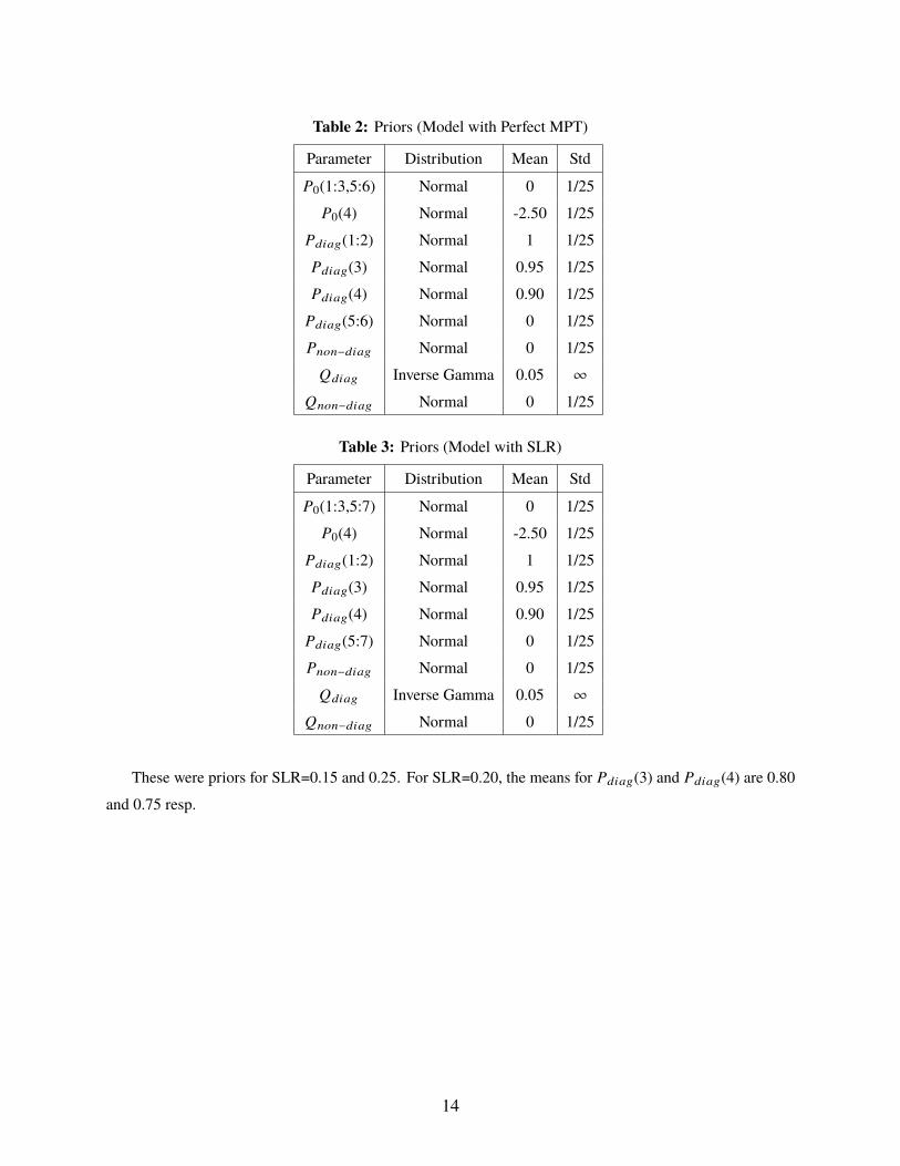
Table 2: Priors (Model with Perfect MPT)

Parameter Distribution Mean Std

%0(1:3,5:6) Normal 0 1/25

%0(4) Normal -2.50 1/25

%3806(1:2) Normal 1 1/25

%3806(3) Normal 0.95 1/25

%3806(4) Normal 0.90 1/25

%3806(5:6) Normal 0 1/25

%=>=−3806 Normal 0 1/25

&3806 Inverse Gamma 0.05 ∞&=>=−3806 Normal 0 1/25

Table 3: Priors (Model with SLR)

Parameter Distribution Mean Std

%0(1:3,5:7) Normal 0 1/25

%0(4) Normal -2.50 1/25

%3806(1:2) Normal 1 1/25

%3806(3) Normal 0.95 1/25

%3806(4) Normal 0.90 1/25

%3806(5:7) Normal 0 1/25

%=>=−3806 Normal 0 1/25

&3806 Inverse Gamma 0.05 ∞&=>=−3806 Normal 0 1/25

These were priors for SLR=0.15 and 0.25. For SLR=0.20, the means for %3806(3) and %3806(4) are 0.80

and 0.75 resp.

14

References[1] Banerjee, Shesadri, Parantap Basu, Chetan Ghate, Pawan Gopalakrishnan, and Sargam Gupta, “A mone-

tary business cycle model for India.,” 2018.[2] Brinca, Pedro, Nikolay Iskrev, and Francesca Loria, “On Identification Issues in Business Cycle Accounting

Models,” MPRA Paper 90250, University Library of Munich, Germany November 2018.[3] , V. V. Chari, Patrick J. Kehoe, and Ellen R. McGrattan, “Accounting for Business Cycles,” Staff Report

531, Federal Reserve Bank of Minneapolis June 2016.[4] Chakraborty, Suparna and Keisuke Otsu, “Business cycle accounting of the BRIC economies,” The BE Journal

of Macroeconomics, 2013, 13 (1), 381–413.[5] Chari, V. V., Patrick J. Kehoe, and Ellen R. McGrattan, “Appendices: Business cycle accounting,” Technical

Report 2006.[6] Chari, Varadarajan V, Patrick J Kehoe, and Ellen R McGrattan, “Business cycle accounting,” Econometrica,

2007, 75 (3), 781–836.[7] Das, Mr Sonali, Monetary policy in India: Transmission to bank interest rates number 15-129, International

Monetary Fund, 2015.[8] Herbst, Edward P and Frank Schorfheide, Bayesian estimation of DSGE models, Princeton University Press,

2015.[9] Lahiri, Amartya and Urjit R Patel, “Challenges of effective monetary policy in emerging economies,” in

“Monetary Policy in India,” Springer, 2016, pp. 31–58.[10] Mishra, Prachi, Peter Montiel, and Rajeswari Sengupta, “Monetary transmission in developing countries:

Evidence from India,” in “Monetary Policy in India,” Springer, 2016, pp. 59–110.[11] Pandey, Radhika, Ila Patnaik, and Ajay Shah, “Dating business cycles in India,” Indian Growth and Develop-

ment Review, 2017, 10 (1), 32–61.[12] Sims, Christopher A, “Solving linear rational expectations models,” Computational economics, 2002, 20 (1),

1–20.[13] Sustek, Roman, “Monetary Business Cycle Accounting,” Review of Economic Dynamics, October 2011, 14 (4),

592–612.[14] Tien, Pao-Lin, Tara M Sinclair, and Edward Gamber, “Do Fed forecast errors matter?,” 2016.

15

A Appendix

A.1 Log-linearized Equations

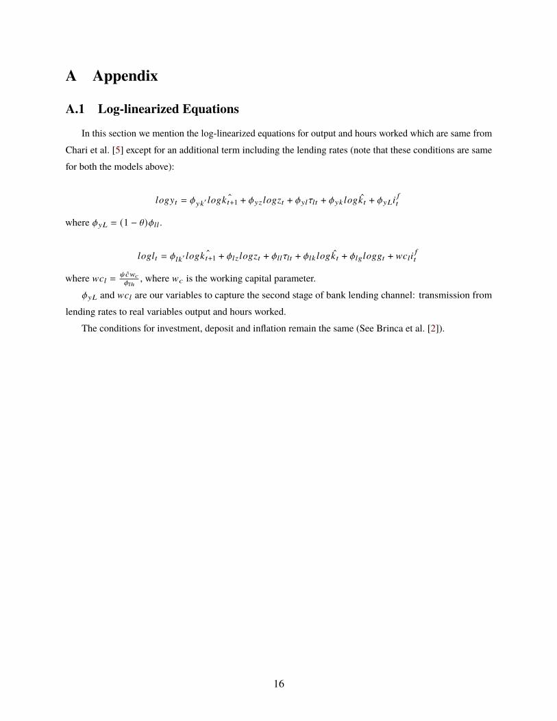
In this section we mention the log-linearized equations for output and hours worked which are same from

Chari et al. [5] except for an additional term including the lending rates (note that these conditions are same

for both the models above):

;>6HC = qH:′ ;>6ˆ:C+1 + qHI ;>6IC + qH;g;C + qH: ;>6:C + qH!8 5C

where qH! = (1 − \)q;;.

;>6;C = q;:′ ;>6ˆ:C+1 + q;I ;>6IC + q;;g;C + q;: ;>6:C + q;6;>66C + F2;8 5C

where F2; = k2F2q;ℎ

, where F2 is the working capital parameter.

qH! and F2; are our variables to capture the second stage of bank lending channel: transmission from

lending rates to real variables output and hours worked.

The conditions for investment, deposit and inflation remain the same (See Brinca et al. [2]).

16

A.2 MLE estimates - Perfect MPT

Table 4: P

0.9748 0.0126 0.0402 0.0009 -0.0039 0.0054

-0.0234 0.9632 0.0218 -0.0054 -0.0029 -0.0390

-0.0120 0.0166 0.9267 0.0002 -0.0045 -0.0087

0.0056 -0.0302 0.0357 0.8215 -0.0035 0.0169

0.0006 0.0033 -0.0029 0.0004 0.1849 0.1442

-0.0118 0.0077 -0.0158 0.0050 0.0188 -0.0333

Table 5: P0

0.0235 -0.0754 0.0826 -0.4565 -0.0002 0.0540

Table 6: Q

0.0266 0.0108 -0.0142 -0.0297 -0.0045 0.0178

0.0108 0.0341 -0.0438 0.1368 -0.0027 -0.0122

-0.0142 -0.0438 0.0134 0.0110 0.0041 -0.0092

-0.0297 0.1368 0.0110 0.3755 0.0006 0.0170

-0.0045 -0.0027 0.0041 0.0006 1.8484 0.1400

0.0178 -0.0122 -0.0092 0.0170 0.1400 0.1084

17

A.3 MLE estimates - SLR (=0.25)

Table 7: P

0.9753 0.0173 0.0433 0.0060 0.0060 0.0208 0.0392

-0.0288 0.9724 0.0159 0.0009 0.0017 -0.0396 -0.0088

-0.0086 0.0248 0.9185 0.0038 0.0005 0.0083 0.0671

0.0050 -0.0306 0.0368 0.8249 0.0024 0.0217 0.0137

0.0016 0.0041 -0.0033 0.0051 0.1926 0.1232 -0.0146

-0.0164 0.0021 -0.0106 0.0018 0.0283 -0.0207 0.0319

-0.0248 -0.0317 0.0307 -0.0030 -0.0006 -0.0258 0.1346

Table 8: P0

0.0215 -0.0796 0.0862 -0.4479 0.0042 0.0524 -0.0010

Table 9: Q

0.0259 0.0102 -0.0121 -0.0287 -0.0026 0.0245 0.0146

0.0102 0.0359 -0.0446 0.1338 0.0069 -0.0075 -0.0061

-0.0121 -0.0446 0.0136 0.0143 0.0061 -0.0095 -0.0011

-0.0287 0.1338 0.0143 0.3730 0.0080 0.0147 0.0080

-0.0026 0.0069 0.0061 0.0080 1.5780 0.1977 0.0453

0.0245 -0.0075 -0.0095 0.0147 0.1977 0.1218 0.0483

0.0146 -0.0061 -0.0011 0.0080 0.0453 0.0483 0.1359

18

A.4 MLE estimates - SLR (=0.15)

Table 10: P

0.9773 0.0193 0.0408 0.0002 0.0095 0.0239 0.0373

-0.0284 0.9715 0.0169 -0.0026 -0.0061 -0.0413 -0.0113

-0.0059 0.0248 0.9236 0.0055 0.0052 0.0065 0.0665

0.0057 -0.0308 0.0370 0.8275 -0.0018 0.0244 0.0193

0.0019 0.0037 -0.0029 0.0030 0.1908 0.1273 -0.0219

-0.0174 0.0031 -0.0108 0.0030 0.0386 -0.0328 0.0413

-0.0235 -0.0312 0.0284 0.0018 -0.0067 -0.0309 0.1499

Table 11: P0

0.0236 -0.0795 0.0860 -0.4401 -0.0095 0.0605 0.0452

Table 12: Q

0.0259 0.0097 -0.0120 -0.0245 0.0044 0.0266 0.0131

0.0097 0.0352 -0.0454 0.1362 0.0079 -0.0092 -0.0099

-0.0120 -0.0454 0.0137 0.0025 0.0102 -0.0084 0.0006

-0.0245 0.1362 0.0025 0.3819 0.0025 0.0163 0.0077

0.0044 0.0079 0.0102 0.0025 1.5715 0.1816 0.0256

0.0266 -0.0092 -0.0084 0.0163 0.1816 0.1256 0.0656

0.0131 -0.0099 0.0006 0.0077 0.0256 0.0656 0.1351

19

Table 13: Decomposition - Perfect MPT

Observable(O) 5$�

5$g; 5$gG 5$�

5$g3 5$'

Output 70.10 5.30 6.70 5.80 6.20 5.90

Hours 25.70 13.10 8.90 19.30 17.00 15.90

Investment 45.30 9.70 13.60 11.10 10.00 10.40

Consumption 21.10 19.70 8.90 17.40 16.10 16.70

Inflation 16.20 16.70 16.70 16.70 17.20 16.40

LR Diff 19.10 28.00 27.40 25.20 0.20 0.30

20

Table 14: Decomposition SLR=0.15

Observable(O) 5$�

5$g; 5$gG 5$�

5$g3 5$'

5$�

Output 66.20 5.10 6.20 5.50 5.80 5.70 5.60

Hours 22.60 11.50 7.80 16.80 14.20 13.90 13.20

Investment 43.20 9.00 11.00 9.80 8.90 9.20 8.90

Consumption 9.50 16.20 13.40 17.60 14.60 14.80 13.90

Inflation 13.60 14.00 14.00 14.00 13.00 13.70 17.50

NIR 6.40 7.30 7.30 7.20 3.20 1.80 66.80

Lending Rate 17.20 20.40 20.20 19.30 1.40 20.60 0.90

Table 15: Decomposition SLR=0.25

Observable(O) 5$�

5$g; 5$gG 5$�

5$g3 5$'

5$�

Output 66.20 5.00 6.30 5.50 5.80 5.70 5.50

Hours 22.90 11.40 7.80 16.70 14.20 13.80 13.10

Investment 42.80 8.90 11.30 9.90 8.90 9.20 9.00

Consumption 9.40 16.30 13.40 17.50 14.60 14.70 14.00

Inflation 13.60 14.00 14.00 14.00 13.30 13.80 17.10

NIR 8.50 9.70 9.80 9.70 4.80 2.30 55.20

Lending Rate 17.20 20.50 20.40 19.40 1.30 20.50 0.80

21

(a) Output per capita (b) Hours

(c) Investment per capita (d) LR Diff

(e) Inflation (f) Lending Rate

Figure 1: Plots of Observables

22

(a) Efficiency Wedge (b) Labor Wedge

(c) Investment Wedge (d) Deposit Wedge

(e) Taylors Rule Wedge

Figure 2: Plots of Wedges

23

(a) Efficiency Wedge (b) Labor Wedge

(c) Investment Wedge (d) Deposit Wedge

(e) Taylors Rule Wedge (f) MPT Wedge

Figure 3: Plots of Wedges - SLR=0.15

24

(a) Efficiency Wedge (b) Labor Wedge

(c) Investment Wedge (d) Deposit Wedge

(e) Taylors Rule Wedge (f) MPT Wedge

Figure 4: Plots of Wedges - SLR=0.25

25