Bus Signal Priority Based on GPS and Wireless Communications

Phase I - Simulation Study

Final Report

Prepared by

Chen-Fu Liao Intelligent Transportation Systems Institute

Center for Transportation Studies University of Minnesota

Gary A. Davis Department of Civil Engineering

University of Minnesota

CTS 06-07

HUMAN CENTERED TECHNOLOGY TO ENHANCE SAFETY AND TECHNOLOGY

Technical Report Documentation Page 1. Report No. 2. 3. Recipients Accession No. CTS 06-07 4. Title and Subtitle 5. Report Date

July 2006 6.

Bus Signal Priority Based on GPS and Wireless Communications Phase I – Simulation Study

7. Author(s) 8. Performing Organization Report No. Chen-Fu Liao and Gary A. Davis 9. Performing Organization Name and Address 10. Project/Task/Work Unit No.

11. Contract (C) or Grant (G) No.

Department of Civil Engineering University of Minnesota 500 Pillsbury Drive SE Minneapolis, MN 55455

CTS Project Number 2005038

12. Sponsoring Organization Name and Address 13. Type of Report and Period Covered Final Report 14. Sponsoring Agency Code

Intelligent Transportation Systems Institute Center for Transportation Studies University of Minnesota 511 Washington Ave. SE #200 Minneapolis, MN 55455

15. Supplementary Notes http://www.cts.umn.edu/pdf/CTS-06-07.pdf 16. Abstract (Limit: 200 words) The Minneapolis-St. Paul metropolitan transit agency has installed Global Positioning System (GPS) equipment in transit vehicles for the purpose of monitoring vehicle locations and schedules in order to provide more reliable transit services. This research project evaluates the potential use of vehicle-mounted GPS to develop a Transit Signal Priority system that improves the efficiency of transit.

Transit Signal Priority (TSP) for transit has been proposed as an efficient way to improve transit travel & operation. Bus signal priority has been implemented in several US cities to provide more reliable travel and improve customer ride quality. Current signal priority strategies implemented in various US cities mostly utilized sensors to detect buses at a fixed or at a preset distance away from the intersection. Signal priority is usually granted after a preprogrammed time offset after detection. The proposed study would take advantage of the GPS system on the buses in Minneapolis and develop a signal priority strategy which could consider the bus’ timeliness with respect to its schedule, its number of passengers, location and speed.

17. Document Analysis/Descriptors 18. Availability Statement Global positioning system, transit, bus priority, traffic signal preemption, wireless communication systems

No restrictions. Document available from: National Technical Information Services, Springfield, Virginia 22161

19. Security Class (this report) 20. Security Class (this page) 21. No. of Pages 22. Price Unclassified Unclassified 86

BUS SIGNAL PRIORITY BASED ON GPS

AND WIRELESS COMMUNICATIONS PHASE I - SIMULATION STUDY

Final Report

Prepared by:

Chen-Fu Liao Senior Systems Engineer

Intelligent Transportation Systems Laboratory Intelligent Transportation Systems Institute and the

Center for Transportation Studies University of Minnesota

Gary A. Davis Professor

Department of Civil Engineering University of Minnesota

July 2006

Intelligent Transportation Systems Institute Center for Transportation Studies

University of Minnesota

CTS 06-07

This report represents the results of research conducted by the authors and does not necessarily reflect the official views or policy of the Center for Transportation Studies or the University of Minnesota.

ACKNOWLEDGEMENTS We would like to thank the Intelligent Transportation Systems (ITS) Institute and Center for Transportation Studies, University of Minnesota, for supporting this project. The ITS Institute is a federally funded program administrated through the United States Department of Transportation (USDOT) Research & Innovative Technology Administration (RITA). We also would like to recognize the following people and organizations for their invaluable assistance in making this research possible.

• Scott Tacheny at City of Minneapolis Public Works Department – for providing traffic data, signal timing plan and numerous discussions and responses to our questions.

• Aaron Isaac, Gary Nyberg, Erin Mitchell at Metro Transit – for providing bus GPS data, schedule and passenger counts information.

• Hun-Wen Tao at the Department of Civil Engineering – for helping us collect traffic data on un-signalized intersections, travel time data and entering traffic data into the simulation model.

• Wu-Ping Xin and John Hourdos at the Department of Civil Engineering – for providing arterial the balancing tool and documentation.

• Ted Morris at the ITS Institute Laboratory – for supporting lab equipments for data collection and traffic simulation tools.

• Pi-Ming Cheng at ITS Institute Intelligent Vehicles Lab – for providing GPS receiver information and geospatial data conversion tool.

• Tony Juettner at Brown Traffic Products, Inc. – for providing information on EPAC traffic controller.

Table of Contents 1. Introduction ……………………………………………………………………………………... 1

1.1 Problem Statement ………………………………………..…………………………... 1 1.2 Background ………………………………………..………………………………...... 1 1.3 Objective ………………………………………..………………………….…………. 2 1.4 Literature Research ………………………………………..…………………………... 2

2. Development of Traffic Simulation Model ….………………………………………………….. 5

2.1 Study Site Selection …………………………………………………………………... 5 2.2 Intersection Capacity Analysis ………………………………………………………... 5

2.3 Data Collection and Calculation ….…………………………………………………… 6 Intersection Signal Timing ……………………………………………………...... 6 Traffic Volume and Turning Movements ………………………………………... 6 Bus Stop Locations ……………………………………………………………….. 7 General Traffic Travel Time ….………………………………………………….. 7 Bus Travel Time ………………………………………………………………….. 8 Bus Delay at Intersection ……………………………………………………….... 9 Bus Dwell Time …………………………………………………………………... 10 2.4 Microscopic Traffic Simulator ….…………………………………………………….. 12

2.5 Network Modeling …………………………………………………………………….. 12 Balancing Arterial Traffic Volumes …………………………………………….... 13 2.6 Network Calibration …………………………………………………………………... 15 Capacity Calibration ….…………………………………………………………... 15 Average Travel Time Validation …………………………………………………. 19 Average Bus Travel Time Validation …………………………………………..... 20 3. Adaptive Bus Signal Priority Strategy ...………………………………………………………... 21 3.1 Bus Signal Priority Request …………………………………………………………... 21 Nearside Bus Stop ………………………………………………………………... 21 Far-side Bus Stop …………………………………………………………………. 22 3.2 Bus Dwell Time Estimation …………………………………………………………... 23 Passenger Arrival Rate at Bus Stop ….…………………………………………… 23

Bus Dwell Time at Bus Stop ……………...…………………………………….... 23 3.3 Bus Signal Priority Acknowledgement ……………………………………………...... 24

Priority Acknowledge Rules ……………………………………………………... 24 Green Extension and Red Truncation …………………………………………….. 25 Signal Recovery/Resynchronization Consideration …………………………….... 25 Current Signal Preemption Settings in Minneapolis ……………………………... 25

3.4 Bus Signal Priority Modeling in the Simulator ……………………………………….. 26 Bus Stop Priority Request ……………………………………………………….... 26 Signal Control Model ….…………………………………………………………. 27

4. Simulation Results Analysis …………………………………………………………………….. 30 4.1 Bus Measures of Effectiveness (MOE) Analysis …………………………………….. 30 AM Peak ….………………………………………………………………………. 31 PM Peak …………………………………………………………………………... 32 4.2 MOE Analysis of Major Intersections ……………………………………………….... 34 Hennepin + Franklin …………………………………………………………….... 34

Lyndale + Franklin …………………………………………………………….…. 34

Nicollet + Franklin …………………………………………………………….…. 34 Chicago + Franklin ……………………………………………………………..... 35 11th + Franklin …………………………………………………………….…….... 35

Cedar + Franklin ……………………………………………………………..…… 36 4.3 Non-Transit Vehicle MOE Analysis ……………………………………………..…… 36

AM Peak …………………………………………………….………………….... 36 PM Peak ………………………………………………………………..……….... 37 4.4 Overall Network System MOE Analysis ……………………………………...…….... 38 AM Peak ………………………………………………………………..……….... 38 PM Peak …………………………………………………………………………... 39 4.5 Potential Saving of Bus Operation …………………………………………………..... 39

5. Future Work …………………………………………………………….……………………….. 40 6. Summary ……………………………………………………………..………………………….. 41 References …………………………………………………………….………………………….... 42 Appendix A: Intersection Signal Timing Plans Appendix B: Bus GPS Data and Conversion Appendix C: Bus Passenger Count and Dwell Time Statistics Appendix D: Arterial Network Balancing Program Appendix E: Traffic Volume Calibration Results

List of Figures Figure 1. Bus Signal Priority Study Site – Franklin Ave From Dupont to 27th Ave …….... 5 Figure 2. Synchro5 Simulation Model of Franklin Avenue ………………………………. 5 Figure 3. Signal Priority Strategy Interface With AIMSUN Simulator ……………….….. 12 Figure 4. Franklin Avenue Network Geometry on Overlaid Aerial Image ……………….. 13 Figure 5. Bus Stops and Detectors Assignment …………………………………………... 13

Figure 6. Traffic Volume Conservation Example ……………………………..………….. 14 Figure 7. AIMSUN Simulation Model of Franklin Avenue …………………..………….. 15 Figure 8. Traffic Volume Calibration – Franklin Ave Eastbound ……………………….... 17

Figure 9. Traffic Volume Calibration – Franklin Ave Westbound ……………………….. 17 Figure 10. An East-West Corridor Example for Signal Priority ………………………….. 21 Figure 11. Poisson Distribution ……….…………………………………………………... 24 Figure 12. Bus Signal Priority Acknowledgement ……….……………………………….. 25

Figure 13. Control Diagram of Bus Signal Priority Strategy ……….…………………….. 26 Figure 14. Flowchart of Bus Signal Priority Control ………………………………….….. 27

Figure 15. Signal Priority Control – Green Extension at Priority Phase ……….……….... 28 Figure 16. Signal Priority Control – Early Green/Red Truncation ……….…………….... 28 Figure 17. Signal Priority Control – Priority Phase Insertion ………………………...….. 29 Figure 18. Overall Network Measures – AM Peak vs. PM Peak ……….………………... 30 Figure 19. AM Peak Bus Speed and Travel Time – Priority vs. No Priority (EXT=10)….. 31 Figure 20. AM Peak Bus Speed and Travel Time – Priority vs. No Priority (EXT=15)….. 32 Figure 21. PM Peak Bus Speed and Travel Time – Priority vs. No Priority (EXT=15)…... 33

List of Tables Table 1. TSP Implementation Experiences in US ………………………………………. 4 Table 2. Intersection LOS ……………………………………………………………..….. 6 Table 3. Intersection capacity utilization (ICU) …………………………………………... 6 Table 4. Intersection Delay ……………………………………………………….……….. 6 Table 5. Observed Travel Time Along Franklin Avenue ……………………………...….. 7 Table 6. Bus Travel Time Extracted From GPS data ……………………………………... 8 Table 7(a). Bus Travel Time From Field Observation – AM Peak ……………………….. 8 Table 7(b). Bus Travel Time From Field Observation – PM Peak ……………………….. 9

Table 8. Bus Delay at Signalized Intersection …………………………………………….. 10 Table 9. Passenger Service Times with Single-Channel Passenger Movement ……….….. 11 Table 10. Passenger Service Times with Multiple-Channel Passenger Movement …...….. 12 Table 11. Capacity Calibration Statistics – AM Peak …………………………………….. 18 Table 12. Capacity Calibration Statistics – PM Peak ……………………………………... 18 Table 13. Capacity Calibration Statistics – Theil’s Coefficients (AM Peak) ………….….. 19 Table 14. Capacity Calibration Statistics – Theil’s Coefficients (PM Peak) ……….…….. 19 Table 15. Average Travel Time Comparisons ……….………………………………….... 20 Table 16. Average Bus Travel Time Comparisons …………………………………....….. 20 Table 17. Franklin Corridor Average Traffic Volume ………………………………...….. 20

Table 18. Network System Statistics – AM Peak vs. PM Peak ……………………….….. 30 Table 19. AM Peak Bus Statistics – Priority vs. No Priority (EXT=10) ……….……….... 31 Table 20. AM Peak Bus Statistics – Priority vs. No Priority (EXT=15) ……….………… 32 Table 21. PM Peak Bus Statistics – Priority vs. No Priority (EXT=15)..……………..…. 33 Table 22. Intersection Statistics –Franklin & Hennepin AM Peak ………………….....…. 34 Table 23. Intersection Statistics –Franklin & Hennepin PM Peak ………………….....…. 34 Table 24. Intersection Statistics –Franklin & Lyndale AM Peak …………………..….…. 34 Table 25. Intersection Statistics –Franklin & Nicollet AM Peak …………………...….…. 35 Table 26. Intersection Statistics –Franklin & Nicollet PM Peak …………………..…..…. 35 Table 27. Intersection Statistics –Franklin & Chicago PM Peak …………………...….…. 35 Table 28. Intersection Statistics –Franklin & 11th PM Peak ………………………......…. 36 Table 29. Intersection Statistics –Franklin & Cedar PM Peak ………………….....……... 36 Table 30. Non-Transit Vehicle AM Statistics – Priority vs. No Priority (EXT=10) ……... 37 Table 31. Non-Transit Vehicle AM Statistics – Priority vs. No Priority (EXT=15) ……... 37 Table 32. Non-Transit Vehicle PM Statistics – Priority vs. No Priority (EXT=15) ……... 38 Table 33. Overall Network AM Statistics – Priority vs. No Priority (EXT=10) ………..... 38 Table 34. Overall Network AM Statistics – Priority vs. No Priority (EXT=15) ………….. 39 Table 35. Overall Network PM Statistics – Priority vs. No Priority (EXT=15) ……...…... 39

Executive Summary Bus operations are influenced by many factors such as traffic congestion, intersection signal delay, and ridership. Providing signal priority for buses has been proposed as an inexpensive way to improve transit efficiency, productivity and reduce operation costs [1]. Bus signal priority has been implemented in several US cities to improve schedule adherence, reduce transit operation costs, and improve customer ride quality [1, 2]. Metro Transit previously performed tests using the 3M™ Opticom™ systems [3] for bus priority on Lake Street. There were significant problems, including triggering timing, and inability to handle nearside bus stops. With the recent installation of GPS/AVL (Automatic Vehicle Location) systems, Metro Transit is monitoring bus locations and schedules in order to provide more reliable transit services and improve service quality. Metro Transit is planning the Northwest Corridor (Bottineau Corridor) project so as to include a bus way that will offer high-quality transit service from downtown Minneapolis through Crystal, Brooklyn Park, Maple Grove and Rogers (http://www.metrotransit.org/improvingTransit/northwestCorridor.asp). In this project, bus signal priority will be considered in order to improve bus travel time and reduce bus delay at signalized intersections. Transit Signal Priority (TSP) conceptual design along Bottineau Corridor is currently being investigated by SEH Inc. As another way to provide transit traveler information, Metro Transit recently initiated a pilot study to investigate customer satisfaction by installing two real-time bus arrival information signs at the Upton Transit Center.

Current signal priority strategies implemented in various US cities mostly utilize sensors to detect buses at a fixed or preset distance away from an intersection. Traditional presence detection systems, ideally designed for emergency vehicles, usually send signal priority request after a preprogrammed time offset as soon as transit vehicles are detected without the consideration of bus readiness. The objective of this study is to take advantage of the already equipped GPS/AVL system on the buses in Minneapolis and develop an adaptive signal priority strategy that could consider the bus schedule adherence, its number of passengers, location and speed. Buses will communicate with intersection signal controllers using wireless technology to request signal priority. Communication with the roadside unit (e.g., traffic controller) for signal priority may be established using the readily available 802.11x WLAN or the DSRC (Dedicated Short Range Communication) 802.11p protocol currently under development for wireless access to and from the vehicular environment.

Bus route #2 in Minneapolis was identified and investigated for providing bus signal priority. A simulation model of traffic conditions along the Franklin Corridor from Dupont to 27th Avenue (about three miles in distance with total of 22 signalized intersections) was created using AIMSUN micro-simulation package (http://www.aimsun.com/). Signalized intersection traffic data and timing plans were obtained from the City of Minneapolis. Traffic volumes and turning movements at un-signalized intersections were collected manually using JAMAR (http://www.jamartech.com/) hand-held traffic counter. Bus schedule and passenger arrivals were modeled using data collected by Metro Transit. The arterial network was then balanced and calibrated to provide a baseline model for priority strategy analysis. The signal priority strategy was developed, implemented using C++ programming language and integrated with the simulator through the AIMSUN API interface. At each simulation step, bus location and its distance corresponding to the next bus stop and signalized intersection were calculated to determine nearside or farside bus stop scenario. Passenger arrival rate was modeled for bus stop dwell time estimation and incorporated into the priority strategy. Signal priority request time was calculated and submitted to controller when bus was ready. Either green signal extension or red light truncation was considered in providing priority for buses.

This phase one study primarily focused on efforts to develop a simulation model in order to investigate the benefit and impact. Simulation results indicate a 12-15% reduction in bus travel time during AM peak hours (7AM-9AM) and 4-11% reduction in PM peak hours (4PM-6PM) could be achieved by providing signal priority for buses. Average bus delay time was reduced in the range of 16-20% and 5-14% during AM and PM peak periods, respectively. The signal priority strategy caused increases of travel time for non-transit vehicles of about 6 seconds per vehicle during AM peak and 22 seconds in PM peak periods in average. The average number of non-transit vehicle stops increased from 1.6 stop/veh to 1.7 stop/veh during AM peak hours and from 2.0 stop/veh to 2.4 stop/veh during PM peak period. Phase II study, submitted to Center for Transportation Studies (CTS) RFP FY-07, is to develop a wireless communication prototype system to verify and validate the signal priority strategy using the GPS/AVL information. The long-term vision of this project is to develop an effective TSP system using wireless communication that Metro Transit can deploy throughout the Twin Cities metro area. Our streets and highways are getting more and more congested as population grows and more cars enter the transportation system. We hope that providing signal priority to buses can help improve quality of transit services, attract more travelers riding public transit and free up space on streets. Furthermore, transit vehicles can potentially be used as probes for determining traffic speeds and travel time along freeways and major arterials [4]. Traffic information can also be integrated and provided to traffic operations or the traveling public.

1

1. INTRODUCTION Transit Signal Priority (TSP) for transit has been studied and proposed as an efficient way to improve transit travel & operation. Bus signal priority has been implemented in several US cities to improve schedule adherence, reduce transit operation costs, and improve customer ride quality. Signal priority strategies have helped reduce the transit travel time delay, as discussed in the literature [1], but the transit travel time reduction varies considerably across studies [2]. Signal priority and preemption are often used synonymously, however, they are different processes. Signal preemption is traditionally used for emergency vehicles (EV) or at railroad crossing. Preemption interrupts normal intersection signal process to provide high priority for special events. Signal priority modifies the normal signal operation in order to accommodate better service for transit vehicles [23]. 1.1 Problem Statement Metro Transit in Twin Cities Metro area (http://www.metrotransit.org/) previously performed an evaluation of providing signal priority for buses on Lake Street in Minneapolis, using 3M™ Opticom™ systems [3]. There were approximately 60 buses equipped with Opticom™ emitters. A special software modification was made to provide transit priority using green extension and red truncation strategies. However, the Opticom™ system, ideally designed for emergency vehicle preemption (EVP), was not able to adjust the triggering timing for buses approaching near-side bus stops and buses often missed the priority green when they were ready to depart. Several intersections along Lake Street were already operating at their capacity, so that there was not much green time available from side streets for bus signal priority. There were also issues of buses traveling across different municipalities that were unwilling to provide signal priority for buses. Results from the previous evaluation study were not promising.

Based on the previous experience, selection of a study site should be considered carefully. In addition, this study would like to take advantage of the already installed GPS/AVL system on the buses operating in Minneapolis, and develop a signal priority strategy that could consider the bus schedule, number of passengers on board, bus location and speed. The first phase of this study will use a simulation model in order to investigate the potential benefits and impacts of a bus priority strategy. 1.2 Background With the recent installation of GPS system on its fleet, Metro Transit is constantly monitoring buses locations in relation to their schedules, in order to provide more reliable transit services and enhance transit operation and management. Bus location, travel time information and other traffic information can also be integrated and provided for traffic operations or to the traveling public.

Transit Signal Priority (TSP) for transit has been proposed as an efficient way to improve transit travel & operation. Bus signal priority has been implemented in several US cities (Seattle, Portland, Los Angeles, Chicago) as well as in Europe. Various technologies have been deployed for bus priority including Opticom™ (St. Cloud) [5], Loopcom (Los Angeles), and RF tag (Seattle, King County) [6]. Recently, Crout [47] at Tri-County Metropolitan Transportation District of Oregon (TriMet) proposed two types of analyses (corridor and intersection level) to evaluate the effectiveness of the TSP effort on transit operations over 300 signals implemented with signal priority.

Metro Transit would prefer to use the already installed GPS/AVL system as the basis of a TSP system. In 2003, 3M unveiled a GPS-based Opticom™ [7] system at the ITS America conference. The system utilized a 2.4GHz frequency-hopping proprietary wireless technology to detect emergency vehicles when they were approaching within about 2,500-ft of an intersection. A Signal preemption request was then sent to the signal controller, based on the vehicle’s heading, position and speed.

2

Current signal priority strategies implemented in various US cities mostly utilized sensors to detect buses at a fixed or at a preset distance away from the intersection. Signal priority is usually granted after a preprogrammed time-offset, after detection. Engineers have to adjust the detector location, receiver line of sight and timing offset for each intersection in order to ensure its effectiveness. These TSP strategies do not consider the bus’s speed and its distance from intersection when determining the appropriate time to request signal priority. The proposed study would like to incorporate the GPS/AVL system on the buses in Minneapolis and develop a signal priority strategy based on the bus’s timeliness with respect to its schedule, number of passengers, location and speed of a bus.

Wireless communications systems have made rapid progress and are commercially available. Bus information (e.g. speed, location, number of passengers, bus ID) can be transmitted wirelessly to a traffic controller or to a regional Traffic Management Center (TMC) in making decisions for signal priority. There are several wireless communication systems installed on each bus under the current Metro Transit setup. An 800-MHz Motorola digital voice radio is used for communication between bus driver and Transit Control Center (TCC). Another 800-MHz analog data radio is used to poll bus location and passenger count data every minute. A Wireless Local Area Network (WLAN) 802.11x is also installed on the bus. This is used to upload/download files between the bus and the TCC central server, when the bus is within the proximity of the transit garage.

With this equipment, transit vehicles could potentially be used as probes for determining traffic speeds and travel times along freeways and major arterials [4]. Real-time traffic data could therefore be transmitted wirelessly to a regional TMC, to adjust the intersection signal or ramp metering timing accordingly. 1.3 Objective With GPS/AVL on the bus, we believe we can provide signal priority to buses with minimal impact on other traffic because GPS offers better information regarding bus trajectory information than other sensors used previously to provide traffic signal priority. Our objective is to investigate the performance of GPS and a wireless-based adaptive signal priority strategy to provide reliable and efficient bus transit services with minimal impact on the other traffic flow. The improved service will hopefully make the transit system more attractive to the public and increase ridership. Simulation studies and field measurements will be used to ensure that the signal priority strategies have no serious negative effect on other traffic. Bus travel time, bus signal delay and cross street traffic delay will be measured and analyzed. 1.4 Literature Research A research group at California PATH (Partners for Advanced Transit and Highways) is pursuing a study titled “Adaptive Bus Signal Priority” (ABSP) to apply an active priority strategy for buses, by including bus GPS information, traffic detector data, and a travel-time predictor to an adaptive model [9]. Yin et al proposed a heuristic TSP algorithm to provide signal priority to buses as well as limit negative impact on cross-street traffic [44]. Traditional TSP strategies implemented in other cities are fixed-location detection systems and implemented with time-of-delay signal control systems. TSP systems using fixed-location detection mostly do not work well with nearside bus stops, due to the uncertainty in bus dwell time. Kim and Rilett [10] proposed a weighted least squares regression model in simulation to estimate bus dwell time in order to overcome nearside bus stop challenges. The ABSP project proposed using GPS for bus detection, a well-defined priority algorithm for priority decision-making, existing loop detectors for real-time traffic data, and microscopic traffic simulation as an evaluation tool. Our proposed strategy will include the estimation of bus arrival time based on the schedule, headway and current location. Nearside or far-side bus stops will also be considered when providing priority to

3

buses. Signal priority strategies, such as green extension or red-truncation, will then be considered based on traffic conditions and the location and speed of the bus.

A bus priority algorithm could also be integrated into an adaptive intersection signal control model. Research based on the bus priority facilities available within the Split Cycle Offset Optimization Technique (SCOOT) [8] traffic signal control system was conducted by Bretherton et al in 1996 [11]. Traffic signal priorities can be controlled by a central SCOOT computer or by a local traffic signal controller. A local controller can achieve faster TSP response to buses than a centralized control. Different strategy options for providing bus priority at signals are compared by McLeod & Hounsell [12] using the simulation model called Selective Priority to Late buses Implemented at Traffic signals (SPLIT). McLeod suggested that differential (conditional) priority strategies (e.g. granting priority for lateness) give the best results, as these provide a good balance between travel time and passengers waiting time. Furth and Mueller [13] conducted a field study with three priority conditions (no priority, absolute priority, conditional priority) at a transit route in the Netherlands. The study found absolute priority caused large delays to other traffic while conditional priority caused little, if any additional delay. Dion and Rakha [46] developed a simulation approach to integrate TSP within an adaptive traffic control system. They evaluate three different signal control scenarios and found adaptive signal control reduced negative impacts on general traffic while providing signal priority to buses. Recently, Mirchandani & Lucas [14] developed a Categorized Arrival-based Phase Reoptimization at Intersection (CAPRI) strategy that integrates transit signal priority within a real-time traffic adaptive signal control system, called RHODES (Real-time Hierarchical Optimized Distributed Effective System) [15]. “Weighted bus” and “phase constrained” approaches were developed for providing transit priority through the RHODES-CAPRI framework. Mirchandani et al [45] proposed a hierarchical optimization approach where traffic signals are determined by considering delays of all vehicles on the network as well as bus passenger counts and schedule while providing transit priority (RHODES/BUSBAND).

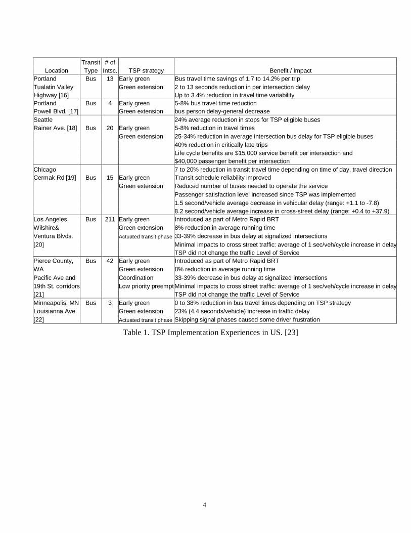
According to the benefit and impact from the implementation results (Table 1) of signal priority for transit vehicles in other cities, overall delay time is reduced and bus on-time performance is improved. In some cases, bus signal priority was associated with an increase in delay for cross street traffic.

As indicated above, we propose to combine GPS information on bus location and speeds, models of bus dwell time based on field observations, and differential consideration of near and far-side bus stops in order to develop an effective bus priority strategy. In its first phase, this strategy will be developed and evaluated using microscopic traffic simulation.

4

Transit # of

Location Type Intsc. TSP strategy Benefit / Impact Portland Bus 13 Early green Bus travel time savings of 1.7 to 14.2% per trip Tualatin Valley Green extension 2 to 13 seconds reduction in per intersection delay Highway [16] Up to 3.4% reduction in travel time variability Portland Bus 4 Early green 5-8% bus travel time reduction Powell Blvd. [17] Green extension bus person delay-general decrease Seattle 24% average reduction in stops for TSP eligible buses Rainer Ave. [18] Bus 20 Early green 5-8% reduction in travel times Green extension 25-34% reduction in average intersection bus delay for TSP eligible buses 40% reduction in critically late trips Life cycle benefits are $15,000 service benefit per intersection and $40,000 passenger benefit per intersection Chicago 7 to 20% reduction in transit travel time depending on time of day, travel direction Cermak Rd [19] Bus 15 Early green Transit schedule reliability improved Green extension Reduced number of buses needed to operate the service Passenger satisfaction level increased since TSP was implemented 1.5 second/vehicle average decrease in vehicular delay (range: +1.1 to -7.8) 8.2 second/vehicle average increase in cross-street delay (range: +0.4 to +37.9) Los Angeles Bus 211 Early green Introduced as part of Metro Rapid BRT Wilshire& Green extension 8% reduction in average running time Ventura Blvds. Actuated transit phase 33-39% decrease in bus delay at signalized intersections [20] Minimal impacts to cross street traffic: average of 1 sec/veh/cycle increase in delay TSP did not change the traffic Level of Service Pierce County, Bus 42 Early green Introduced as part of Metro Rapid BRT WA Green extension 8% reduction in average running time Pacific Ave and Coordination 33-39% decrease in bus delay at signalized intersections 19th St. corridors Low priority preempt Minimal impacts to cross street traffic: average of 1 sec/veh/cycle increase in delay [21] TSP did not change the traffic Level of Service Minneapolis, MN Bus 3 Early green 0 to 38% reduction in bus travel times depending on TSP strategy Louisianna Ave. Green extension 23% (4.4 seconds/vehicle) increase in traffic delay [22] Actuated transit phase Skipping signal phases caused some driver frustration

Table 1. TSP Implementation Experiences in US. [23]

5

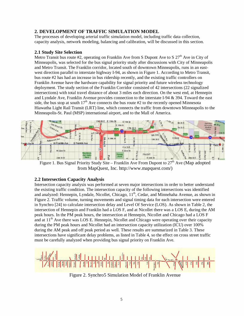
2. DEVELOPMENT OF TRAFFIC SIMULATION MODEL The processes of developing arterial traffic simulation model, including traffic data collection, capacity analysis, network modeling, balancing and calibration, will be discussed in this section. 2.1 Study Site Selection Metro Transit bus route #2, operating on Franklin Ave from S Dupont Ave to S 27th Ave in City of Minneapolis, was selected for the bus signal priority study after discussions with City of Minneapolis and Metro Transit. The Franklin corridor, located south of downtown Minneapolis, runs in an east-west direction parallel to interstate highway I-94, as shown in Figure 1. According to Metro Transit, bus route #2 has had an increase in bus ridership recently, and the existing traffic controllers on Franklin Avenue have the hardware capability for signal priority and future wireless technology deployment. The study section of the Franklin Corridor consisted of 42 intersections (22 signalized intersections) with total travel distance of about 3 miles each direction. On the west end, at Hennepin and Lyndale Ave, Franklin Avenue provides connection to the interstate I-94 & 394. Toward the east side, the bus stop at south 17th Ave connects the bus route #2 to the recently opened Minnesota Hiawatha Light Rail Transit (LRT) line, which connects the traffic from downtown Minneapolis to the Minneapolis-St. Paul (MSP) international airport, and to the Mall of America.

Figure 1. Bus Signal Priority Study Site – Franklin Ave From Dupont to 27th Ave (Map adopted

from MapQuest, Inc. http://www.mapquest.com/) 2.2 Intersection Capacity Analysis Intersection capacity analysis was performed at seven major intersections in order to better understand the existing traffic condition. The intersection capacity of the following intersections was identified and analyzed: Hennepin, Lyndale, Nicollet, Chicago, 11th, Cedar, and Minnehaha Avenue, as shown in Figure 2. Traffic volume, turning movements and signal timing data for each intersection were entered in Synchro [24] to calculate intersection delay and Level Of Service (LOS). As shown in Table 2, the intersection of Hennepin and Franklin had a LOS F, and at Nicollet there was a LOS E, during the AM peak hours. In the PM peak hours, the intersection at Hennepin, Nicollet and Chicago had a LOS F and at 11th Ave there was LOS E. Hennepin, Nicollet and Chicago were operating over their capacity during the PM peak hours and Nicollet had an intersection capacity utilization (ICU) over 100% during the AM peak and off peak period as well. These results are summarized in Table 3. These intersections have significant delay problems, as listed in Table 4, so the effect on cross street traffic must be carefully analyzed when providing bus signal priority on Franklin Ave.

Figure 2. Synchro5 Simulation Model of Franklin Avenue

6

Franklin Avenue - Intersection LOS Intersection AM Peak Off Peak PM Peak Hennepin F C F Lyndale D C C Nicollet E B F Chicago C D F 11th B D E Cedar C B D Minnehaha B B B

Table 2. Intersection LOS

Franklin Avenue - Intersection Capacity Utilization Intersection AM Peak Off Peak PM Peak Hennepin 94.9% 69.4% 116.0% Lyndale 96.7% 72.1% 88.5% Nicollet 117.9% 113.6% 162.7% Chicago 77.9% 86.8% 121.3% 11th 64.0% 62.8% 99.2% Cedar 57.3% 47.0% 83.7% Minnehaha 47.4% 46.3% 68.6%

Table 3. Intersection capacity utilization (ICU)

Franklin Avenue - Intersection Delay (sec) Intersection AM Peak Off Peak PM Peak Hennepin 183.4 27.6 148.0 Lyndale 47.2 39.0 39.4 Nicollet 86.8 25.0 676.2 Chicago 33.8 49.5 202.5 11th 23.1 51.8 84.3 Cedar 25.9 19.1 64.3 Minnehaha 14.3 11.3 16.9

Table 4. Intersection Delay

2.3 Data Collection and Calculation Intersection Signal Timing Signal timing plans for the signalized intersections were provided by the City of Minneapolis, Public Works department. The signal timing plans included AM-peak (6:00-8:45), PM-peak (15:00-18:30) and off-peak hours, and are listed in Appendix A. Traffic Volume and Turning Movements Traffic volume and turning movements per 15-minute period at the signalized intersections were obtained from the City of Minneapolis. At the time of the study, Minneapolis did not have traffic data for the un-signalized intersections. The 15-minute traffic volume and turning movements at the un-signalized intersections were manually collected using a JAMAR [25] handheld traffic counter, during

7

the morning (7:00-9:00) and afternoon (16:00-18:00) peak periods. Vehicle hourly volume and turning proportions in percentage were then calculated and entered into the AIMSUN simulation model. Bus Stop Locations Metro Transit provided bus stop location data in GPS latitude-longitude format (See Appendix B.1). The North American Datum of 1983 (NAD 1983) was used to convert the GPS data into the Minnesota south state plane coordinate system (SPCS), MN-S 2203. The MnCON [26] software tool, developed by MnDOT to perform conversions between mapping projections and coordinate systems used in the state of Minnesota, was used to convert the bus GPS data into state plane XY coordinates. MnCON also has the capability of converting between projections based on different datums using the National Geodetic Survey’s NADCON algorithm [27]. Converted bus stop coordinates were then placed accordingly in the simulation network geometry (Figure 4). General Traffic Travel Time Franklin Avenue travel time: A floating vehicle, making 3 round trips during both the AM and PM peak hours, was used to measure average travel time along Franklin Avenue. The average travel time, as listed in Table 5, was collected with 1-minute resolution. The morning traffic along Franklin was lighter as compared to that in the afternoon. The average travel time during the AM peak hours was about 3 minutes shorter than that of PM peak hours. Travel time data will later be used to adjust the baseline model travel time in the simulation.

Franklin Ave Travel Times - Observed Start Time End Time Duration Direction hh:mm hh:mm minute Eastbound 7:14 7:24 10 Westbound 7:27 7:34 7

A.M. Eastbound 7:44 7:52 8 Westbound 7:55 8:04 9 Eastbound 8:14 8:23 9 Westbound 8:25 8:34 9 Eastbound Average 9.00 Westbound Average 8.33 Start Time End Time Duration Direction hh:mm hh:mm minute Westbound 4:14 4:26 12 Eastbound 4:28 4:38 10

P.M. Westbound 4:41 4:54 13 Eastbound 5:02 5:16 14 Westbound 5:20 5:33 13 Eastbound 5:34 5:44 10 Eastbound Average 11.33 Westbound Average 12.67

Table 5. Observed Travel Time Along Franklin Ave.

8

Bus Travel Time Based on the collected data, a substantial portion of bus travel time was spent decelerating for bus stops, waiting for passenger boarding and alighting, waiting to re-enter the traffic stream, and accelerating. Buses usually do not reach their maximum attainable cruise speeds between stops when operating on city streets because of traffic congestion, intersection interference, or traffic signal control. Bus travel time extracted from GPS data: The average travel time for buses was computed using the per-minute bus GPS data. The data set from Metro Transit included 5 days of bus GPS data of route #2. A Java program was developed to extract the data collected on Franklin Ave. during the AM and PM peak hours. A listing of the program is included in Appendix B.2. Listings of bus travel times calculated from the GPS data are tabulated in Appendix B.3. The average bus travel time for both east and westbound is shown in Table 6.

Average Bus From Bus GPS data Travel Time EB WB AM Peak (sec) 1177 1048

(mm:ss) 19:37 17:28 PM Peak (sec) 1204 1206

(mm:ss) 20:04 20:06 Table 6. Bus Travel Time Extracted From GPS data

Bus travel time from field observation: In addition to the estimates of the bus travel times from the GPS data, field observations were performed by taking several bus trips during both peak hours, along Franklin Ave. The collected data are shown in Table 7, from which average travel times were calculated. Measured bus travel times will be compared to that from the simulation model in order to verify the accuracy of the public transit model used in the simulator.

Start Time End Time Duration Direction hh:mm hh:mm minute Eastbound 7:46 8:08 22 Eastbound 8:47 9:06 19 Eastbound 7:03 7:22 19 Eastbound 7:51 8:15 24 Eastbound 8:23 8:43 20 Eastbound 8:47 9:06 19

AM Eastbound 9:34 9:55 21 PEAK Eastbound Average 20.57

Westbound 7:14 7:31 17 Westbound 8:13 8:30 17 Westbound 7:40 7:57 17 Westbound 8:06 8:27 21 Westbound 8:21 8:39 18 Westbound 8:44 9:02 18 Westbound 9:15 9:34 19 Westbound Average 18.14

Table 7(a). Bus Travel Time From Field Observation – AM Peak

9

Start Time End Time Duration Direction hh:mm hh:mm minute Eastbound 4:56 5:18 22 Eastbound 3:54 4:13 19 Eastbound 4:11 4:32 21 Eastbound 4:33 4:51 18 Eastbound 5:09 5:31 22 Eastbound 5:39 5:59 20

PM Eastbound Average 20.33 PEAK Westbound 4:26 4:47 21

Westbound 5:34 5:52 18 Westbound 3:49 4:08 19 Westbound 4:11 4:32 21 Westbound 4:43 5:04 21 Westbound 5:09 5:32 23 Westbound 5:27 5:45 18 Westbound 5:42 6:02 20 Westbound 6:25 6:42 17 Westbound 6:45 7:05 20 Westbound Average 19.80

Table 7(b). Bus Travel Time From Field Observation – PM Peak Bus Delay at Intersection The purpose of providing signal priority to transit a vehicle is to minimize its waiting time at intersections. It is important to know how much time buses spend waiting at red lights as compared to their total travel times. Collecting the bus delay times at red signals will provide information on the degree of improvement that bus signal priority could provide to the existing bus operation. Based on the collected data shown in Table 8, buses traveling westbound take, on average, about 18 minutes with approximately 210 seconds of delay at red signals. Buses traveling in the eastbound direction average about 20 minutes, including about 260 seconds of signal delay per trip. By comparing the average intersection delay to the average bus travel time, a bus generally spent on average around 18% to 23% of its travel time (3.3~4.8 minutes) waiting for green lights at intersection along Franklin Avenue.

10

Franklin Ave Bus Signal Delay - Observed

Travel Time Signal Delay Signal Delay Direction minute second % Westbound 17 221 21.67% Eastbound 22 347 26.29%

A.M. Westbound 17 173 16.96% Eastbound 19 278 24.39% Westbound 19 204 17.89% Eastbound 21 232 18.41% Westbound Average 17.67 199.33 18.84% Eastbound Average 20.67 285.67 23.03% Travel Time Signal Delay Signal Delay Direction minute second % Westbound 21 241 19.13% Eastbound 22 290 21.97%

P.M. Westbound 18 172 15.93% Eastbound 18 257 23.80% Westbound 15 245 27.22% Eastbound 18 170 15.74% Westbound Average 18.00 219.33 20.76% Eastbound Average 19.33 239.00 20.50%

Table 8. Bus Delay at Signalized Intersection Bus Dwell Time Bus dwell time at each bus stop includes the boarding/alighting of passengers, door opening/closing and clearance time. The per-minute bus GPS data provided by Metro Transit does not provide sufficient resolution for us to calculate and estimate the bus dwell time at each bus stop. Also, Metro Transit was not able to provide passenger counts at the time of this study using the APC (automatic passenger count) unit integrated with the bus GPS/AVL data collection system along Franklin Avenue. However, Metro Transit conducted passenger boarding/alighting counts at every bus stop along bus route #2 from 6AM to 12AM during 2000 and 2001. Bus dwell time at each stop can therefore be calculated using the recommended formulas from Transit Capacity and Quality of Service Manual [28].

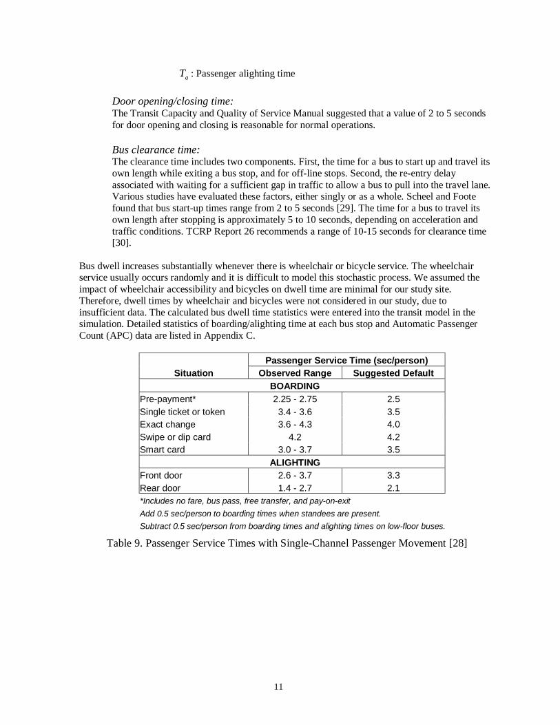
Boarding/alighting time: This time can be estimated using values given in Table 9 for typical operating conditions: single-door loading, pay on bus, or Table 10 for multiple channel passenger movement:

alightingboardingT / = bC bT + aC aT (1) Where,

alightingboardingT / : Passenger boarding/alighting time

bC : Boarding passenger counts

bT : Passenger boarding time

aC : Alighting passenger counts

11

aT : Passenger alighting time

Door opening/closing time: The Transit Capacity and Quality of Service Manual suggested that a value of 2 to 5 seconds for door opening and closing is reasonable for normal operations.

Bus clearance time: The clearance time includes two components. First, the time for a bus to start up and travel its own length while exiting a bus stop, and for off-line stops. Second, the re-entry delay associated with waiting for a sufficient gap in traffic to allow a bus to pull into the travel lane. Various studies have evaluated these factors, either singly or as a whole. Scheel and Foote found that bus start-up times range from 2 to 5 seconds [29]. The time for a bus to travel its own length after stopping is approximately 5 to 10 seconds, depending on acceleration and traffic conditions. TCRP Report 26 recommends a range of 10-15 seconds for clearance time [30].

Bus dwell increases substantially whenever there is wheelchair or bicycle service. The wheelchair service usually occurs randomly and it is difficult to model this stochastic process. We assumed the impact of wheelchair accessibility and bicycles on dwell time are minimal for our study site. Therefore, dwell times by wheelchair and bicycles were not considered in our study, due to insufficient data. The calculated bus dwell time statistics were entered into the transit model in the simulation. Detailed statistics of boarding/alighting time at each bus stop and Automatic Passenger Count (APC) data are listed in Appendix C.

Passenger Service Time (sec/person)

Situation Observed Range Suggested Default BOARDING Pre-payment* 2.25 - 2.75 2.5 Single ticket or token 3.4 - 3.6 3.5 Exact change 3.6 - 4.3 4.0 Swipe or dip card 4.2 4.2 Smart card 3.0 - 3.7 3.5 ALIGHTING Front door 2.6 - 3.7 3.3 Rear door 1.4 - 2.7 2.1 *Includes no fare, bus pass, free transfer, and pay-on-exit Add 0.5 sec/person to boarding times when standees are present. Subtract 0.5 sec/person from boarding times and alighting times on low-floor buses.

Table 9. Passenger Service Times with Single-Channel Passenger Movement [28]

12

Available Default Passenger Service Time (sec/person)

Door Channels Boarding* Front Alighting Rear Alighting 1 2.5 3.3 2.1 2 1.5 1.8 1.2 3 1.1 1.5 0.9 4 0.9 1.1 0.7 6 0.6 0.7 0.5

*Assumes no on-board fare payment required *Increase boarding times by 20% when standees are present. *For low-floor buses, reduce boarding times by 20%, front alighting times by 15%, and rear alighting times by 25%.

Table 10. Passenger Service Times with Multiple-Channel Passenger Movement [28] 2.4 Microscopic Traffic Simulator A microscopic traffic simulation package, AIMSUN (Advanced Interactive Microscopic Simulator for Urban and Non-urban Networks, http://www.aimsun.com) [31] was selected for this study. AIMSUN is embedded in GETRAM (Generic Environment for TRaffic Analysis and Modeling), a simulation environment inspired by modern trends in the design of graphical user interfaces adapted to traffic modeling requirements [31]. GETRAM comprises a traffic network graphical editor (TEDI), a network database, a module for storing results, and an Application Programming Interface (API) to allow interfacing to other simulation or assignment models. An additional library of DLL (Dynamic Link Library) functions (GETRAM Extensions) enables the system to communicate with external applications [31, 32]. AIMSUN has been used successfully for numerous large-scale traffic modeling research projects within the ITS lab [33] and provides a well-documented API to access and modify all elements of the simulation state (signal control, sensing, vehicle characteristics and state) while the simulation is running. A C++ program was developed to interface with the microsimulator through the GETRAM API. As shown in Figure 3, bus location, speed, and bus stop information can be sent to the external bus signal priority application, and a priority request can be sent back to the simulator, in real-time.

Figure 3. Signal Priority Strategy Interface With AIMSUN Simulator

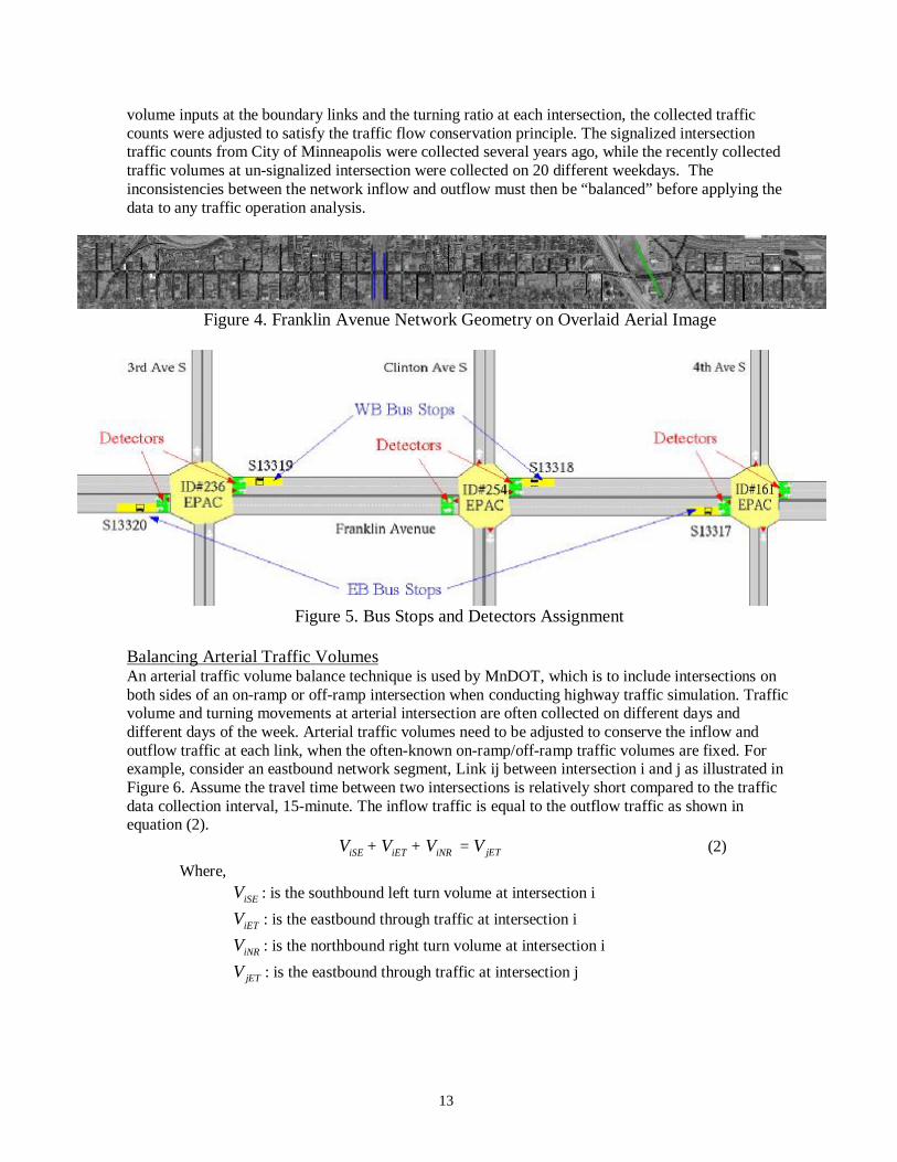
2.5 Network Modeling Digital Orthophotos Quad aerial images (DOQs) around Franklin Avenue were acquired from Twin Cities Metropolitan Council (http://www.datafinder.org/metadata/orthos2000.htm). The aerial images were then used to create the arterial network geometry for the AIMSUN simulation model, as shown in Figure 4. Bus route and bus stop locations were selected and specified in the network geometry (Figure 5) and bus dwell time statistics were entered in the transit model. Intersection signal timing and phase assignments were specified in the signal control model. Three different vehicle types, passenger car, light truck, and bus, were included in the simulation model. The 15-minute traffic volume and turning proportions collected at each intersection were entered. Before entering the traffic

13

volume inputs at the boundary links and the turning ratio at each intersection, the collected traffic counts were adjusted to satisfy the traffic flow conservation principle. The signalized intersection traffic counts from City of Minneapolis were collected several years ago, while the recently collected traffic volumes at un-signalized intersection were collected on 20 different weekdays. The inconsistencies between the network inflow and outflow must then be “balanced” before applying the data to any traffic operation analysis.

Figure 4. Franklin Avenue Network Geometry on Overlaid Aerial Image

Figure 5. Bus Stops and Detectors Assignment

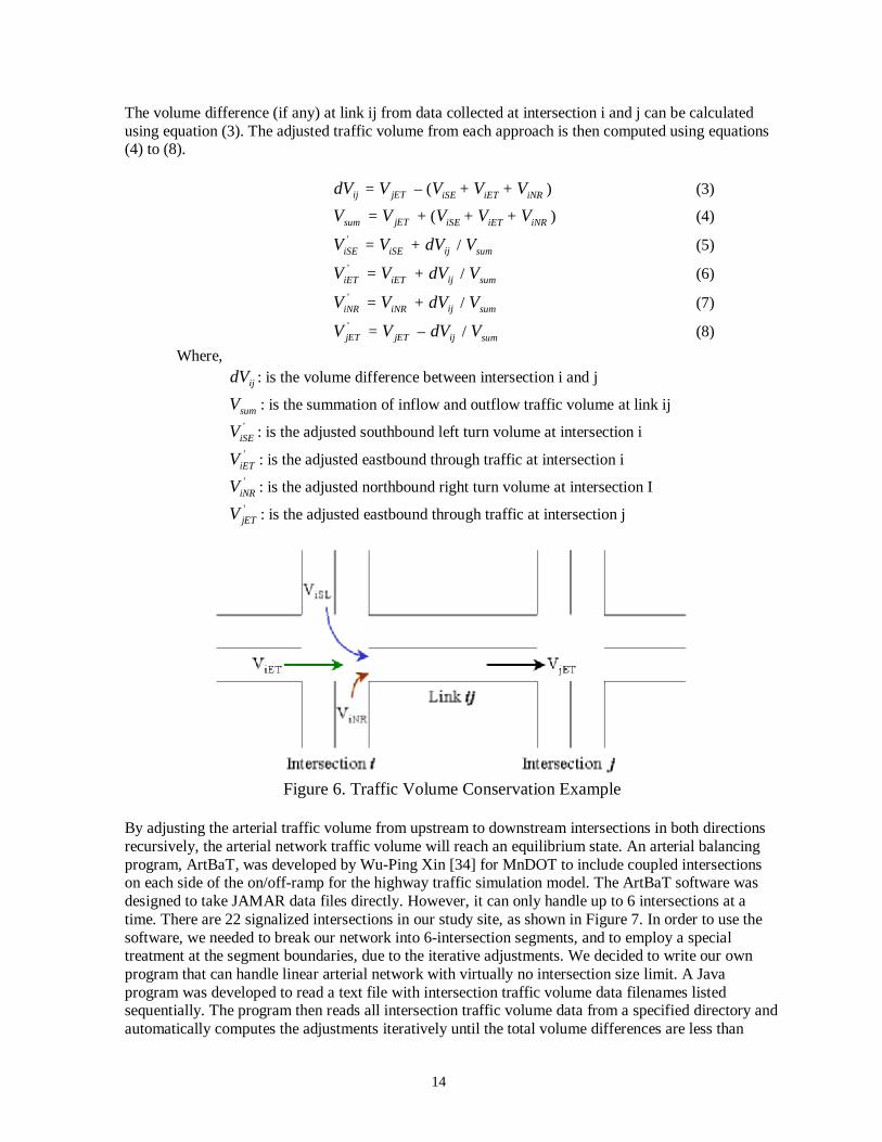
Balancing Arterial Traffic Volumes An arterial traffic volume balance technique is used by MnDOT, which is to include intersections on both sides of an on-ramp or off-ramp intersection when conducting highway traffic simulation. Traffic volume and turning movements at arterial intersection are often collected on different days and different days of the week. Arterial traffic volumes need to be adjusted to conserve the inflow and outflow traffic at each link, when the often-known on-ramp/off-ramp traffic volumes are fixed. For example, consider an eastbound network segment, Link ij between intersection i and j as illustrated in Figure 6. Assume the travel time between two intersections is relatively short compared to the traffic data collection interval, 15-minute. The inflow traffic is equal to the outflow traffic as shown in equation (2). iSEV + iETV + iNRV = jETV (2) Where, iSEV : is the southbound left turn volume at intersection i iETV : is the eastbound through traffic at intersection i iNRV : is the northbound right turn volume at intersection i jETV : is the eastbound through traffic at intersection j

14

The volume difference (if any) at link ij from data collected at intersection i and j can be calculated using equation (3). The adjusted traffic volume from each approach is then computed using equations (4) to (8). ijVδ = jETV – ( iSEV + iETV + iNRV ) (3)

sumV = jETV + ( iSEV + iETV + iNRV ) (4)

'iSEV = iSEV + ijVδ / sumV (5)

'iETV = iETV + ijVδ / sumV (6)

'iNRV = iNRV + ijVδ / sumV (7)

'jETV = jETV – ijVδ / sumV (8)

Where, ijVδ : is the volume difference between intersection i and j

sumV : is the summation of inflow and outflow traffic volume at link ij

'iSEV : is the adjusted southbound left turn volume at intersection i

'iETV : is the adjusted eastbound through traffic at intersection i

'iNRV : is the adjusted northbound right turn volume at intersection I

'jETV : is the adjusted eastbound through traffic at intersection j

Figure 6. Traffic Volume Conservation Example

By adjusting the arterial traffic volume from upstream to downstream intersections in both directions recursively, the arterial network traffic volume will reach an equilibrium state. An arterial balancing program, ArtBaT, was developed by Wu-Ping Xin [34] for MnDOT to include coupled intersections on each side of the on/off-ramp for the highway traffic simulation model. The ArtBaT software was designed to take JAMAR data files directly. However, it can only handle up to 6 intersections at a time. There are 22 signalized intersections in our study site, as shown in Figure 7. In order to use the software, we needed to break our network into 6-intersection segments, and to employ a special treatment at the segment boundaries, due to the iterative adjustments. We decided to write our own program that can handle linear arterial network with virtually no intersection size limit. A Java program was developed to read a text file with intersection traffic volume data filenames listed sequentially. The program then reads all intersection traffic volume data from a specified directory and automatically computes the adjustments iteratively until the total volume differences are less than

15

0.01. The balanced traffic volume for each intersection is then stored in the specified directory with .csv (comma separated value) file format. The results of the raw versus balanced traffic volume are plotted in Appendix D.1 and D.2 for AM and PM peak periods, respectively. The Java program and a sample input text file are included in Appendix D. 2.6 Network Calibration When the intersection traffic data were balanced and entered in the AIMSUN simulation model for each 15-minute interval, an error-checking task was performed by running a trial simulation run in order to visually identify any unusual traffic condition. For example, incorrect intersection signal phasing or offset may cause unusual queue buildup. A working model of Franklin Avenue is available for calibration upon the completion of the error-checking tasks. The traffic simulation model can only include a portion of all parameters that affect the real-world traffic conditions. The calibration process helps improve the ability of traffic model to accurately reproduce the local traffic conditions [35].

Figure 7. AIMSUN Simulation Model of Franklin Avenue

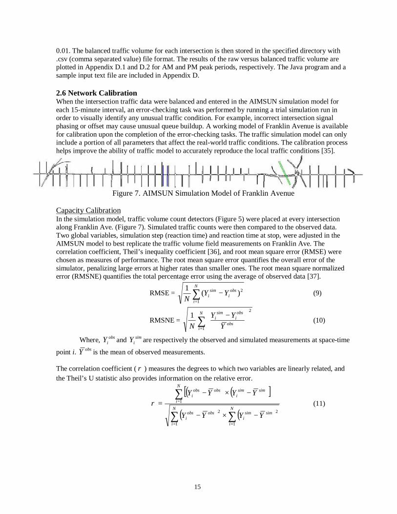
Capacity Calibration In the simulation model, traffic volume count detectors (Figure 5) were placed at every intersection along Franklin Ave. (Figure 7). Simulated traffic counts were then compared to the observed data. Two global variables, simulation step (reaction time) and reaction time at stop, were adjusted in the AIMSUN model to best replicate the traffic volume field measurements on Franklin Ave. The correlation coefficient, Theil’s inequality coefficient [36], and root mean square error (RMSE) were chosen as measures of performance. The root mean square error quantifies the overall error of the simulator, penalizing large errors at higher rates than smaller ones. The root mean square normalized error (RMSNE) quantifies the total percentage error using the average of observed data [37].

RMSE = ∑=

−N

i

obsi

simi YY

N 1

2)(1 (9)

RMSNE = ∑=

−N

iobs

obsi

simi

YYY

N 1

21

(10)

Where, obsiY and sim

iY are respectively the observed and simulated measurements at space-time

point i. obsY is the mean of observed measurements. The correlation coefficient ( ρ ) measures the degrees to which two variables are linearly related, and the Theil’s U statistic also provides information on the relative error.

( ) ( )[ ]

( ) ( )∑ ∑

∑

= =

=

−×−

−×−=

N

i

N

i

simsimi

obsobsi

N

i

simsimi

obsobsi

YYYY

YYYY

1 1

22

1ρ (11)

16

( )

( ) ( )∑∑

∑

==

=

+

−=

N

i

obsi

N

i

simi

N

i

obsi

simi

YN

YN

YYNU

1

2

1

2

1

2

11

1

(12)

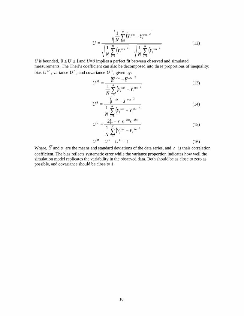
U is bounded, 10 ≤≤ U and U=0 implies a perfect fit between observed and simulated measurements. The Theil’s coefficient can also be decomposed into three proportions of inequality: bias MU , variance SU , and covariance CU , given by:

( )

( )∑=

−

−= N

i

obsi

simi

obssimM

YYN

YYU

1

2

2

1 (13)

( )

( )∑=

−

−= N

i

obsi

simi

obssimS

YYN

U

1

2

2

1σσ

(14)

( )

( )∑=

−

−= N

i

obsi

simi

obssimC

YYN

U

1

2112 σσρ

(15)

1=++ CSM UUU (16) Where, Y and σ are the means and standard deviations of the data series, and ρ is their correlation coefficient. The bias reflects systematic error while the variance proportion indicates how well the simulation model replicates the variability in the observed data. Both should be as close to zero as possible, and covariance should be close to 1.

17

08:00 ~ 08:15AM EBReaction Time = 0.75s, Reaction Time at Stop = 0.8s

0

50

100

150

200

250

1 3 5 7 9 11 13 15 17 19 21 23 25 27 29 31 33 35 37 39 41

Detector Station (42 intersections)

15-m

in V

olum

e

EB SIM EB BAL

Figure 8. Traffic Volume Calibration – Franklin Ave Eastbound

08:00 ~ 08:15AM WBReaction Time = 0.75s, Reaction Time at Stop = 0.8s

0

20

40

60

80

100

120

140

160

1 3 5 7 9 11 13 15 17 19 21 23 25 27 29 31 33 35 37 39 41

Detector Station (42 intersections)

15-m

in V

olum

e

WB SIM WB BAL

Figure 9. Traffic Volume Calibration – Franklin Ave Westbound

18

Sample simulated and observed traffic volumes for the 42 intersections, from 8:00AM to 8:15AM are plotted in Figure 8 and 9. The calibration statistics are listed in Table 11, 12, 13 and 14. Lists of detector stations and further traffic volume calibration results are included in Appendix E.

Correlation, ρ Theil's coefficient, U RMSE RMSNE AM Peak EB WB EB WB EB WB EB WB 7:15 AM 0.9835 0.9366 0.0520 0.0813 7.6306 8.7460 11.97% 18.06% 7:30 AM 0.9877 0.9094 0.0338 0.0658 6.5422 9.0776 7.32% 12.93% 7:45 AM 0.9826 0.9862 0.0430 0.0469 9.7262 9.4233 9.21% 10.08% 8:00 AM 0.9850 0.9346 0.0324 0.0454 8.8377 10.4287 7.00% 9.33% 8:15 AM 0.9569 0.9089 0.0502 0.0548 12.5094 11.6682 10.50% 11.49% 8:30 AM 0.9842 0.9638 0.0470 0.0847 11.7012 18.6164 10.26% 18.98% 8:45 AM 0.9905 0.9422 0.0351 0.0513 8.1470 10.5897 7.39% 10.49% 9:00 AM 0.9730 0.9285 0.0632 0.0500 13.8079 9.9312 12.84% 10.49%

Average 0.9804 0.9388 0.0446 0.0600 9.8628 11.0601 9.56% 12.73% STD DEV 0.0108 0.0261 0.0107 0.0155 2.5626 3.1921 2.21% 3.74%

Table 11. Capacity Calibration Statistics – AM Peak

Correlation, ρ Theil's coefficient, U RMSE RMSNE

PM Peak EB WB EB WB EB WB EB WB 4:15 PM 0.9663 0.9856 0.0394 0.0363 11.4076 12.7511 8.18% 7.64% 4:30 PM 0.9854 0.9675 0.0370 0.0409 11.3274 15.4853 7.48% 8.62% 4:45 PM 0.9699 0.9429 0.0585 0.0502 18.7050 18.9980 11.77% 10.05% 5:00 PM 0.9707 0.9645 0.0382 0.0301 13.3188 12.3484 8.07% 6.07% 5:15 PM 0.9890 0.9772 0.0597 0.0283 20.2412 11.9268 11.86% 5.68% 5:30 PM 0.9543 0.9826 0.0448 0.0341 16.0244 14.2796 9.28% 6.73% 5:45 PM 0.9648 0.8945 0.0578 0.0349 20.0140 13.6602 12.55% 7.09% 6:00 PM 0.9648 0.9571 0.0738 0.0518 23.7536 19.4253 16.16% 11.02%

Average 0.9707 0.9590 0.0511 0.0383 16.8490 14.8593 10.67% 7.86% STD DEV 0.0114 0.0296 0.0133 0.0087 4.5651 2.9153 2.96% 1.90%

Table 12. Capacity Calibration Statistics – PM Peak

19

Theil's bias, Um Theil's variance, Us Theil's covariance, Uc

AM Peak EB WB EB WB EB WB 7:15 AM 0.4392 0.5299 0.0013 0.0967 0.5732 0.3847 7:30 AM 0.0441 0.3457 0.0441 0.2405 0.8767 0.4907 7:45 AM 0.0923 0.6468 0.1889 0.1546 0.7321 0.2090 8:00 AM 0.0739 0.0004 0.0309 0.1967 0.8953 0.9161 8:15 AM 0.0266 0.0920 0.0923 0.0040 0.8788 1.0205 8:30 AM 0.0406 0.7308 0.5063 0.1208 0.5180 0.1924 8:45 AM 0.0223 0.0741 0.5690 0.1493 0.4097 0.8374 9:00 AM 0.4557 0.0974 0.1640 0.0014 0.3749 0.9972

Average 0.1493 0.3146 0.1996 0.1205 0.6573 0.6310 STD DEV 0.1855 0.2889 0.2189 0.0850 0.2161 0.3506

Table 13. Capacity Calibration Statistics – Theil’s Coefficients (AM Peak)

Theil's bias, Um Theil's variance, Us Theil's covariance, Uc PM Peak EB WB EB WB EB WB 4:15 PM 0.0147 0.7947 0.0805 0.0117 0.9048 0.2162 4:30 PM 0.5835 0.6005 0.0060 0.0134 0.4234 0.4352 4:45 PM 0.3727 0.2258 0.2702 0.2549 0.3663 0.6107 5:00 PM 0.2118 0.1188 0.0921 0.1792 0.7273 0.8166 5:15 PM 0.7869 0.4330 0.0700 0.0006 0.1427 0.6313 5:30 PM 0.0141 0.6900 0.0678 0.0460 0.9099 0.2504 5:45 PM 0.5453 0.0186 0.0980 0.0039 0.3881 1.1163 6:00 PM 0.4815 0.7751 0.2985 0.0139 0.2174 0.2401

Average 0.3763 0.4571 0.1229 0.0654 0.5100 0.5396 STD DEV 0.2778 0.3049 0.1038 0.0967 0.2992 0.3188

Table 14. Capacity Calibration Statistics – Theil’s Coefficients (PM Peak) Average Travel Time Validation Average travel time was collected by using a floating vehicle traveling from Dupont Ave to 26th Avenue, for eastbound traffic, and from 27th Ave to Hennepin Ave for westbound traffic, during the AM and PM peak periods. Collected data were then compared with the travel time from simulation, as tabulated in Table 15. The traffic along Franklin Corridor in the simulation model took 43 seconds longer traveling in eastbound and 94 seconds longer traveling in westbound than the observed travel time during AM peak hours. In the PM peak hours, traffic in the simulation model took 24 seconds longer traveling in eastbound direction, but the westbound travel time in the simulation was 27 seconds shorter than the travel time collected from the field. Because the travel time from field observation were collected and recorded in minutes, the travel time differences between the simulator and observation data were within the +/- 1-minute accuracy.

20

Average Travel Time (mm:ss) AM Peak Observed Simulated Difference

EB 09:00 09:43 00:43 WB 08:20 09:54 01:34

Average Travel Time (mm:ss)

PM Peak Observed Simulated Difference EB 11:20 11:44 00:24 WB 12:40 12:13 00:27

Table 15. Average Travel Time Comparisons Average Bus Travel Time Validation Bus dwell times at stops, delays at intersections, and traffic congestion contribute significant variation to bus travel time. The average bus travel times extracted from the GPS data, from field observations, and from the traffic simulation are listed in Table 16. The observed bus travel times were mostly longer than the times extracted from bus GPS data, except in the westbound direction during the PM peak hours. Bus travel time from the AIMSUN simulator during the AM peak hours in the eastbound direction was about 41 seconds shorter (westbound about 53 seconds longer) than the field observation. However, buses in the simulation model took slightly longer time (about 1.5 minutes) in the PM peak period to travel along the Franklin Avenue as compared to the observed data.

Average Bus Travel Time (mm:ss) AM Peak Observed Simulated

EB 20:34 19:53 WB 18:09 19:02

Average Bus Travel Time (mm:ss)

PM Peak Observed Simulated EB 20:20 21:43 WB 19:48 21:17

Table 16. Average Bus Travel Time Comparisons

As shown in Table 17, the average traffic volumes during the PM peak hours were significantly higher than that the AM peak hours (50% and 110% increase). Due to the significant increase of traffic volume in PM peak hours, excess bus travel time was mostly caused by: (1) the re-entry delay associated with waiting for a sufficient gap in traffic to allow a bus to pull back to the travel lane, and (2) queue delay associated with waiting for a stopped queue to clear and allow a bus to enter the bus bay.

Average Traffic Volume veh/h EB WB A.M. 418 362 P.M. 627 759

Table 17. Franklin Corridor Average Traffic Volume

21

3. ADAPTIVE BUS SIGNAL PRIORITY STRATEGY 3.1 Bus Signal Priority Request To illustrate our priority strategy, consider a simple eastbound/westbound corridor as shown in Figure 10. For a bus approaching a bus stop or signalized intersection, there are basically two scenarios, a nearside bus stop or a far-side bus stop. For the nearside bus stop, a bus will stop for boarding/alighting before passing the signalized intersection, as illustrated in Figure 10 eastbound bus approaching stop j and intersection i. Estimated bus dwell time at the nearside bus stop needs to be considered for the signal controller to provide signal priority to the bus in a timely manner. For the far-side bus stop, a bus has to pass through the intersection first before its arrival at the stop (see Figure 10 westbound bus approaching intersection i and bus stop k). Bus travel time to the intersection needs to be considered when providing priority.

Figure 10. An East-West Corridor Example for Signal Priority

Nearside Bus Stop Consider the bus traveling in the eastbound as shown in Figure 10. Expected bus dwell time, djT , at

bus stop j can be forecasted using historical dwell time statistics. Average bus travel time, ajT , from its current location to bus stop can be calculated via,

delaybrb

jeaj TT

vd

T ++×

=467.1

, (17)

Where, bv : is bus speed, in MPH, jed , : is the distance from the current bus location to bus stop j, in feet,

brT : is bus braking/stopping time. Typical values are around 6 ~ 7 seconds, assuming a bus speed of 35 MPH, bus deceleration of 10 ft/s/s, with 1 to 2 seconds of recognition and reaction time,

delayT : is the traffic delay on bus route. The average bus travel time ( jiT ) from bus stop j to intersection i can also be calculated as follows, assuming the distance from the nearside bus stop to the intersection is relatively short compared to the distance needed to accelerate to running speed.

22

bcjeie

ji Ta

ddT +

−=

)(2 ,, (18)

Where, ied , : is the distance from eastbound bus to intersection i (ft),

jed , : is the distance from eastbound bus to bus stop j (ft), a : is the bus acceleration in ft/s/s.

bcT : is the bus clearance time. (Bus waiting time to find sufficient gap to enter to the travel lane.)

Therefore the predicted time for the eastbound bus passing intersection i can be calculated as follows. jidjajei TTTtt +++=ˆ (19) Where,

t : is the current time, sec.

And estimated time for the bus leaving stop j is, djajlj TTtt ++=ˆ (20)

The desired signal priority request should be sent at nδ seconds prior to the bus departure time at stop

j. That is, at time nljt δ−ˆ .

constcommcpn ttt ++=δ (21) Where, cpt : is the controller processing time,

commt : is the communication latency time, constt : is a time constant.

The signal priority service can therefore be ended at xiei Tt +ˆ , where xiT is the time for the bus to cross

intersection i. If both beginning ( nljt δ−ˆ ) and ending ( xiei Tt +ˆ ) of the estimated priority service fall

within the green split, no action needs to be taken at the controller. If nljt δ−ˆ falls in the green split

and xiei Tt +ˆ falls in the red split, extended green time is needed to ensure that bus could pass the

intersection. However, if the estimated beginning of priority service time ( nljt δ−ˆ ) falls within the red light period, red signal truncation or early green light treatment is needed to provide bus signal priority. Far-side Bus Stop For a bus approaching an intersection prior to its arrival at next bus stop, for example, the bus traveling in westbound as shown in Figure 10, signal priority should be provided based on bus traveling speed. The estimated time ( aiT ) to arrive at intersection i can be calculated as,

delayb

iwai T

vd

T +×

=467.1

, (22)

Where, iwd , : is the distance from westbound bus to intersection i (ft),

23

bv : is bus speed in MPH,

delayT : is the traffic delay on bus route. Therefore the estimated time for westbound bus passing intersection i can be calculated as follows. aiwi Ttt +=ˆ (23) Where,

t : is the current time, sec.

The desired signal priority would need to begin at nδ seconds prior to the bus arriving intersection i

( nwit δ−ˆ ), where nδ is defined as equation (21). The signal priority service can be ended at xiwi Tt +ˆ ,

where xiT is the time for bus to cross intersection i. If both beginning ( nwit δ−ˆ ) and ending ( xiwi Tt +ˆ ) of the estimated priority service fall within the green split, no action needs to be taken by the controller. If nwit δ−ˆ falls in the green split and xiwi Tt +ˆ falls in the red split, extended green time is need to ensure bus could pass the intersection. However, if the estimated beginning of priority service time ( nwit δ−ˆ ) falls within the red light period, red signal truncation or early green light treatment is needed to offer bus priority. 3.2 Bus Dwell Time Estimation In order to provide information to riders on expected bus arrival times, many researchers have developed models for bus travel time prediction. Reinhoudt and Velastin [38] proposed a dynamic algorithm to predict bus travel time using the Kalman filter. Dailey, Wall, Maclean and Cathey [39] created a prediction algorithm that uses historical statistics in an optimal filtering framework (Kalman filter) to predict bus arrivals. Shalaby and Farhan [40] developed a passenger arrival rate prediction model using the Kalman filter. Predicted bus dwell time can simply be obtained by multiplying the predicted passenger arrival rate by the predicted bus headway and by the passenger boarding time. Discussion of estimation of bus travel time, arrival time, or departure time is outside the scope of this study. However, the prediction model of bus dwell time is discussed.

Passenger Arrival Rate at Bus Stop Based on the collected data, we assume the passenger arrivals at each stop follow a Poisson distribution as shown in Figure 11 with an arrival rate, λ , calculated from the mean of the collected passenger arrival rate. A Poisson process subroutine was developed to generate numbers of passengers boarding and alighting at each stop during the simulation.

Bus Dwell Time at Bus Stop Bus dwell time at a bus stop for boarding can be estimated using the following equation.

[ ] boardingkkjB

dj TjtjttT ×−×= − )()()( 1λ (24) Where, B

djT is the bus dwell time for boarding at stop j,

)(tjλ is the passenger arrival rate for stop j,

)( jtk is the arrival time of bus k at stop j, )(1 jtk− is the arrival time of bus k-1 at stop j, boardingT is the average boarding time per passenger.

24

Poisson Distribution(Lambda=3)

0.000

0.050

0.100

0.150

0.200

0.250

1 3 5 7 9 11 13 15

Number of Passenger

Prob

abili

ty

Figure 11. Poisson Distribution

3.3 Bus Signal Priority Acknowledgement After receiving a signal priority request from a bus, the signal controller has to determine whether or not to grant the request. Only one bus will get the priority service if there are multiple requests at the same intersection from buses in different approaches. The signal controller will ignore all bus priority requests if there is an emergency vehicle preemption request.

Priority Acknowledgement Rules The signal controller will consider the following three components when determining which bus will receive the priority service. For example, consider two buses A and B, requesting for priority within the same cycle, as shown in Figure 12.

I. Priority request time, TF (Time Factor)

( )

>==<==

=BAT

BAT

ttWBAttBWA

BATF,1

1,,

Bus A wins if it requests earlier than bus B does, where TW is the request time weighting factor ( 1≥TW ).

II. Bus schedule adherence, LF (Lateness Factor)

LateL TWLF ×= Where LW is the bus late time weighting factor ( 1≥LW ) and LateT is the number of minute the bus was late. 0=LF when bus is ahead of its schedule.

III. Number of passengers on the bus, PF (Passenger Factor)

passengerP NWPF ×=

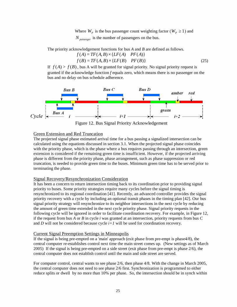
25

Where PW is the bus passenger count weighting factor ( 1≥PW ) and

passengerN is the number of passengers on the bus. The priority acknowledgement functions for bus A and B are defined as follows.

)}()({),()( APFALFBATFAf +×= )}()({),()( BPFBLFBATFBf +×= (25)

If )()( BfAf > , bus A will be granted for signal priority. No signal priority request is granted if the acknowledge function f equals zero, which means there is no passenger on the bus and no delay on bus schedule adherence.

Figure 12. Bus Signal Priority Acknowledgement

Green Extension and Red Truncation The projected signal phase estimated arrival time for a bus passing a signalized intersection can be calculated using the equations discussed in section 3.1. When the projected signal phase coincides with the priority phase, which is the phase where a bus requires passing through an intersection, green extension is considered if the remaining green time is insufficient. However, if the projected arriving phase is different from the priority phase, phase arrangement, such as phase suppression or red truncation, is needed to provide green time to the buses. Minimum green time has to be served prior to terminating the phase. Signal Recovery/Resynchronization Consideration It has been a concern to return intersection timing back to its coordination prior to providing signal priority to buses. Some priority strategies require many cycles before the signal timing is resynchronized to its regional coordination [41]. Recently, an advanced controller provides the signal priority recovery with a cycle by including an optional transit phases in the timing plan [42]. Our bus signal priority strategy will resynchronize to its neighbor intersections in the next cycle by reducing the amount of green time extended in the next cycle priority phase. Signal priority requests in the following cycle will be ignored in order to facilitate coordination recovery. For example, in Figure 12, if the request from bus A or B in cycle i was granted at an intersection, priority requests from bus C and D will not be considered because cycle i+1 will be used for coordination recovery. Current Signal Preemption Settings in Minneapolis If the signal is being pre-empted on a 'main' approach (exit phase from pre-empt is phase4/8), the central computer re-establishes control next time the main street comes up. (New settings as of March 2005) If the signal is being pre-empted on a side street (exit phase from pre-empt is phase 2/6), the central computer does not establish control until the main and side street are served.

For computer control, central wants to see phase 2/6, then phase 4/8. With the change in March 2005, the central computer does not need to see phase 2/6 first. Synchronization is programmed to either reduce splits or dwell by no more than 10% per phase. So, the intersection should be in synch within

26

5 cycles, and it is observed that it is usually within 3 cycles. The maximum time for all emergency vehicle preemptions is 90-second in Minneapolis. Currently City of Minneapolis does not provide signal priority for buses. 3.4 Bus Signal Priority Modeling in the Simulator The priority strategy was implemented using the C++ programming language and integrated with the simulator through the AIMSUN API interface. At each simulation step, the bus location and its distance corresponding to the next bus stop and signalized intersection were calculated to determine nearside or far side bus stop scenario. The control diagram for the priority strategy is shown in Figure 13. Bus dwell time at each stop was computed based on the passenger arrival using the Poisson distribution. Bus travel time to the intersection and bus stop was calculated to determine when to submit priority request prior to its arrival at the signalized intersection.

Figure 13. Control Diagram of Bus Signal Priority Strategy

Bus Stop Priority Requests For the far side bus stop scenario, priority request time was determined by subtracting the estimated bus arrival time at the intersection from a predefined look-ahead time (system response time). For nearside bus stop situations, the priority request was triggered when a bus is within a predefined distance (system response distance). Calculated bus arrival time and dwell time at the bus stop were sent to the priority controller to determine when to submit the priority request. When a priority request is granted, the controller in the simulator calculates the current signal timing and phasing and determines the exit and re-entry phases using green extension or red truncation methodologies. The flowchart of the signal priority control logic was shown in Figure 14.

27

Figure 14. Flowchart of Bus Signal Priority Control Signal Control Model External signal control logic was programmed to emulate the green extension and red truncation functionality. In order to ensure that the intersection returns back to its timing plan prior to the priority request and remains coordinated with the neighboring intersections, signal timing recovery and resynchronization were also considered. Several strategies were discussed as follows.

1. Extend green and maintain coordination: For example, consider a scenario as shown in Figure 15, where priority request occurred during phase 1. Because the current signal phase is the priority phase for buses, the control will simply extend additional green time for the current phase and reduce the same amount of green time from the following phase. In this case, the priority phase (1) stole green time from its next phase and the signal timing remained coordinated with other intersections.

Read intersectionand bus stop data

Acquire bus(k) location,compare its distance to

next stop(j) and intersection(i)

dist2NextStop>dist2NextIntsc ?

Far side bus stop Nearside bus stop

Estimate time when buswill pass next signalized

intersection

t_estimate - sim_time<= system response time ?

No

Estimate bus dwell, arrivaltime at bus stop and travel

time to next intersection

dist2BusStop <=system response distance ?

Submit priority requestusing green extensionor red truncation for

intersection (i)

No

NoYes

Yes Yes

Exit extension phase and return back to phasep+1, where p is the phase before extension

Resynchronize signaltiming at next cycle

GETRAM APIInterface

TrafficSimulator

Is intersection (i)priority enabled ?

Yes

No Wait for next signalizedintersection with enabled

signal priority strategy

Read intersectionand bus stop data

Acquire bus(k) location,compare its distance to

next stop(j) and intersection(i)

dist2NextStop>dist2NextIntsc ?

Far side bus stop Nearside bus stop

Estimate time when buswill pass next signalized

intersection

t_estimate - sim_time<= system response time ?

No

Estimate bus dwell, arrivaltime at bus stop and travel

time to next intersection

dist2BusStop <=system response distance ?

Submit priority requestusing green extensionor red truncation for

intersection (i)

No

NoYes

Yes Yes

Exit extension phase and return back to phasep+1, where p is the phase before extension

Resynchronize signaltiming at next cycle

GETRAM APIInterface

TrafficSimulator

Is intersection (i)priority enabled ?

Yes

No Wait for next signalizedintersection with enabled

signal priority strategy

28

Figure 15. Signal Priority Control – Green Extension at Priority Phase

2. Early green or red truncation:

When the priority request occurred during the phase (4) prior to the priority phase (1), as depicted in Figure 16, the controller will cause an early termination of the current phase and introduce the priority phase earlier. The current phase gave up its remaining green time to the priority phase. The timing plan remains synchronized with other intersections.

Figure 16. Signal Priority Control – Early Green/Red Truncation

3. Phase insertion and coordination recovery in next cycle:

When the priority request occurred after the priority phase was recently serviced, a phase insertion was introduced to the control in order to provide signal priority to the buses as shown in Figure 17. The inserted phase will cause disruption of the signal coordination with the neighboring controllers. A green time reduction from the priority in the next cycle is performed to bring the timing plan back to synchronization.

29

Figure 17. Signal Priority Control – Priority Phase Insertion

The control logic for signal timing resynchronization can be described in computer language as follows.

delta_time = remaining_time – extension_time ; if (delta_time>0) { if (priority request occurred at transition phase) { update priority phase duration d to d+delta_time ; } else if (current_phase != priority phase) { update duration of phase requested priority p to p+delta_time ;

} } else if (delta_time<0) {

update priority phase duration d to d+delta_time ; }

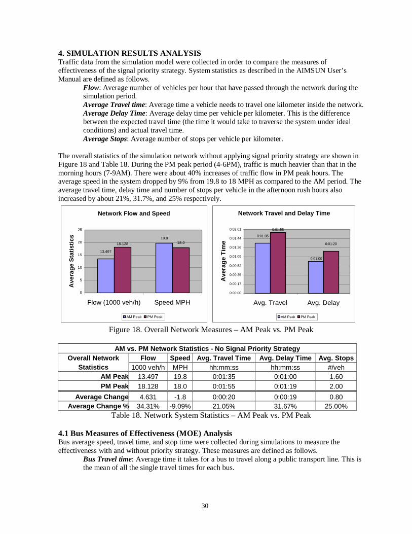
30

4. SIMULATION RESULTS ANALYSIS Traffic data from the simulation model were collected in order to compare the measures of effectiveness of the signal priority strategy. System statistics as described in the AIMSUN User’s Manual are defined as follows.

Flow: Average number of vehicles per hour that have passed through the network during the simulation period. Average Travel time: Average time a vehicle needs to travel one kilometer inside the network. Average Delay Time: Average delay time per vehicle per kilometer. This is the difference between the expected travel time (the time it would take to traverse the system under ideal conditions) and actual travel time. Average Stops: Average number of stops per vehicle per kilometer.

The overall statistics of the simulation network without applying signal priority strategy are shown in Figure 18 and Table 18. During the PM peak period (4-6PM), traffic is much heavier than that in the morning hours (7-9AM). There were about 40% increases of traffic flow in PM peak hours. The average speed in the system dropped by 9% from 19.8 to 18 MPH as compared to the AM period. The average travel time, delay time and number of stops per vehicle in the afternoon rush hours also increased by about 21%, 31.7%, and 25% respectively.

Network Flow and Speed

19.818.0

13.497

18.128

0

5

10

15

20

25

Flow (1000 veh/h) Speed MPH

Ave

rage

Sta

tistic

s

AM Peak PM Peak

Network Travel and Delay Time

0:01:35

0:01:00

0:01:55

0:01:20

0:00:00

0:00:17

0:00:35

0:00:52

0:01:09

0:01:26

0:01:44

0:02:01

Avg. Travel Avg. Delay

Ave

rage

Tim

e

AM Peak PM Peak

Figure 18. Overall Network Measures – AM Peak vs. PM Peak

AM vs. PM Network Statistics - No Signal Priority Strategy

Overall Network Flow Speed Avg. Travel Time Avg. Delay Time Avg. Stops Statistics 1000 veh/h MPH hh:mm:ss hh:mm:ss #/veh

AM Peak 13.497 19.8 0:01:35 0:01:00 1.60 PM Peak 18.128 18.0 0:01:55 0:01:19 2.00

Average Change 4.631 -1.8 0:00:20 0:00:19 0.80 Average Change % 34.31% -9.09% 21.05% 31.67% 25.00%

Table 18. Network System Statistics – AM Peak vs. PM Peak 4.1 Bus Measures of Effectiveness (MOE) Analysis Bus average speed, travel time, and stop time were collected during simulations to measure the effectiveness with and without priority strategy. These measures are defined as follows.

Bus Travel time: Average time it takes for a bus to travel along a public transport line. This is the mean of all the single travel times for each bus.

31

Bus Delay Time: Average delay time per bus to make the trip. This is the difference between the expected travel time (time it takes to go from the origin to the destination under ideal conditions) and the actual travel time. Bus Stop Time: Average time spent at a stop per bus during the trip.

AM Peak Bus statistics from the simulation with and without signal priority strategy are listed in Tables 19 & 20 for AM peak hours. Bus travel time and speed are also plotted in Figure 19 & 20. Two cases were studied in the AM peak period. A maximum green time extension of 15 seconds and 10 seconds were respectively studied to compare the bus travel time reduction and traffic delay. It took about 20(19) minutes for a EB (WB) bus to travel between Hennepin Ave and 27th Ave on Franklin Ave without applying signal priority. By applying the signal priority strategy with maximum green extension of 10 seconds for the buses, the bus travel time was reduced by about 2 minutes in EB and 1.5 minutes in WB direction, or 10% in EB and 8.5% in WB, respectively. Bus delay time was reduced by about 11%~13% and the stop time was reduced around 14%~15% as well.

Priority Extension Time = 10 sec

AM PEAK Speed Bus Travel Time Bus Delay Time Bus Stop Time Bus Statistics MPH hh:mm:ss hh:mm:ss hh:mm:ss

No EB 9.1 0:19:53 0:14:49 0:10:05 Priority WB 9.2 0:19:08 0:14:08 0:09:30

With EB 10.2 0:17:54 0:12:50 0:08:34 Priority WB 10.1 0:17:30 0:12:29 0:08:08 Average EB 1.10 - 0:01:59 - 0:01:59 - 0:01:31 Change WB 0.90 - 0:01:38 - 0:01:39 - 0:01:22 Average EB 12.09% -9.97% -13.39% -15.04%

Change % WB 9.78% -8.54% -11.67% -14.39% Table 19. AM Peak Bus Statistics– Priority vs. No Priority (EXT=10)

AM Peak Bus Speed

9.1

10.2

9.2

10.1

8.4

8.6

8.8

9

9.2

9.4

9.6

9.8

10

10.2

10.4

No Priority With Priority

Ave

rage

Spe

ed M

PH

EB WB

AM Peak Bus Travel Time

0:17:540:17:30

0:19:53

0:19:02

0:14:24

0:15:07

0:15:50

0:16:34

0:17:17

0:18:00

0:18:43

0:19:26

0:20:10

No Priority With Priority

Trav

el T

ime

EB WB

Figure 19. AM Peak Bus Speed and Travel Time – Priority vs. No Priority (EXT=10)

A 15-second maximum green time extension scenario was examined to further investigate the potential of bus travel time reduction. The bus travel time was reduced by about 2.5 minutes in both directions, i.e., 12% in EB and 13.6% in WB. There was on average an additional 1-minute (0.5-

32

minute) travel time reduction for EB (WB) buses from the 10-second scenario discussed previously. By applying the signal priority strategy with a maximum green extension of 15 seconds for the buses, the bus travel time was reduced by about 12% in EB and 14% in WB, respectively. Bus delay time was reduced by about 16%~19% and the stop time was reduced around 18% as well.

Public Transit, Priority Extension Time = 15 sec AM PEAK Speed Bus Travel Time Bus Delay Time Bus Stop Time

Bus Statistics MPH hh:mm:ss hh:mm:ss hh:mm:ss No EB 9.1 0:19:53 0:14:49 0:10:05

Priority WB 9.2 0:19:08 0:14:08 0:09:30 With EB 10.4 0:17:30 0:12:26 0:08:17

Priority WB 10.7 0:16:27 0:11:27 0:07:50 Average EB 1.30 - 0:02:23 - 0:02:23 - 0:01:48 Change WB 1.50 - 0:02:41 - 0:02:41 - 0:01:40 Average EB 14.29% -11.99% -16.09% -17.85%

Change % WB 16.30% -14.02% -18.99% -17.54% Table 20. AM Peak Bus Statistics – Priority vs. No Priority (EXT=15)

AM Peak Bus Speed

9.1

10.4

9.2

10.7

8

8.5

9

9.5

10

10.5

11

No Priority With Priority

Ave

rage

Spe

ed M

PH

EB WB

AM Peak Bus Travel Time

0:16:27

0:19:53

0:17:30

0:19:02

0:14:24

0:15:07

0:15:50

0:16:34

0:17:17

0:18:00

0:18:43

0:19:26

0:20:10

No Priority With Priority

Trav

el T

ime

EB WB

Figure 20. AM Peak Bus Speed and Travel Time – Priority vs. No Priority (EXT=15)

A 20-second maximum green time extension scenario was also investigated. However, it did not yield an additional bus travel time reduction, but did cause more traffic delay and stops. Impacts for general traffic resulting from providing bus signal priority will be discussed in section 4.2. PM Peak As discussed previously, there was about a 40% increase in traffic flow during the PM peak hours. Bus statistics from the simulation with and without signal priority strategy are listed in Table 21 for PM peak hours. Bus travel time and speed are also plotted in Figure 21. A maximum green time extension of 15 seconds was studied to compare the effectiveness of the signal priority strategy with heavier traffic condition, as compared to the AM peak period. In the PM peak hours, it took about 22(23) minutes for a EB (WB) bus to travel between Hennepin Ave and 27th Ave on Franklin Ave without signal priority. By applying the signal priority strategy for the buses, the bus travel time was reduced by about 2 minutes in EB and 1.5 minutes in WB direction, or 10.5% in EB and 7% in WB,

33

respectively. Bus delay time was reduced by about 9%~14% and the stop time was reduced around 10%~14% as well.

As the simulation results shown, the signal priority strategy during the PM peak hours provided relatively less travel time reduction in WB (about 1-minute less) as compared to the AM scenario. There were mostly nearside bus stops at our study site. During the PM peak hours, there were longer queues at intersections from 11th Ave to Cedar Avenue, so that a bus was not able to get in to its service bay when it approached a queue at the intersection. The bus stuck behind the queue had to wait until the queue cleared at the next green in order to provide service. Also, when there was a queue built up during the bus service period at a nearside bus stop, the bus had to wait to find an acceptable gap in order to join the traffic. The priority request will help clear the queue to reduce bus clearance time. However, if knowledge of the queue length could be obtained and processed to submit priority request earlier, the bus waiting time can be reduced during the busier PM period. Future enhancements to the priority strategy can include consideration of queue detection at the intersection.

Public Transit, Priority Extension Time = 15 sec PM PEAK Speed Bus Travel Time Bus Delay Time Bus Stop Time

Bus Statistics MPH hh:mm:ss hh:mm:ss hh:mm:ss No EB 8.3 0:21:58 0:16:55 0:10:14

Priority WB 7.7 0:22:41 0:17:41 0:10:10 With EB 9.2 0:19:39 0:14:35 0:09:15

Priority WB 8.3 0:21:03 0:16:02 0:08:47 Average EB 0.90 - 0:02:19 - 0:02:20 - 0:00:59 Change WB 0.60 - 0:01:38 - 0:01:39 - 0:01:23 Average EB 10.84% -10.55% -13.79% -9.61%

Change % WB 7.79% -7.20% -9.33% -13.61% Table 21. PM Peak Bus Statistics– Priority vs. No Priority (EXT=15)

PM Peak Bus Speed

9.2

7.7

8.38.3

6.5

7

7.5

8

8.5

9

9.5

No Priority With Priority

Ave

rage

Spe

ed M

PH

EB WB

PM Peak Bus Travel Time

0:21:580:22:41

0:19:39

0:21:03

0:14:24

0:15:50

0:17:17

0:18:43

0:20:10

0:21:36

0:23:02

0:24:29

No Priority With Priority

Trav

el T

ime

EB WB

Figure 21. PM Peak Bus Speed and Travel Time – Priority vs. No Priority (EXT=15)

34

4.2 MOE Analysis of Major Intersections Major intersection measures of effectiveness were analyzed and discussed. From Table 2, there were 5 intersections having LOS D or higher during AM and PM peak hours. Hennepin & Franklin The intersection of Franklin and Hennepin previously had LOS F during both AM and PM peak hours. The average vehicle travel time and delay time did not change during AM peak hours with the priority strategy as listed in Table 22 & 23. The average number stops per vehicle decreased by 0.03 stops/veh. During the PM peak hours, there were 1.5 sec and 1.0 sec decreases in average travel time and vehicle delay, respectively. Average stops per vehicle increased slightly by 0.01.

AM Peak - Franklin & Hennepin Intersection Flow Speed Travel Time Delay Time Avg. Stops

Statistics veh/h MPH mm:ss mm:ss #/veh No Priority 606.50 24.59 00:57.5 01:20.0 0.33

With Priority 605.00 24.86 00:57.5 01:20.0 0.30 Average Change -1.50 0.28 00:00.0 00:00.0 -0.03

Average Change % -0.25% 1.12% 0.00% 0.00% -7.69% Table 22. Intersection Statistics –Franklin & Hennepin AM Peak

PM Peak - Franklin & Hennepin

Intersection Flow Speed Travel Time Delay Time Avg. Stops Statistics veh/h MPH mm:ss mm:ss #/veh

No Priority 675.00 25.78 01:01.0 01:26.0 0.28 With Priority 673.13 25.66 00:59.5 01:25.0 0.29

Average Change -1.875 -0.11 - 00:01.5 - 00:01.0 0.01 Average Change % -0.28% -0.44% -2.46% -1.16% 4.55%

Table 23. Intersection Statistics –Franklin & Hennepin PM Peak

Lyndale & Franklin During the AM peak hours at the Franklin and Lyndale intersection (LOS D in AM peak without signal priority), average vehicle travel time and delay decreased respectively by 8.5 sec and 16 sec when applying signal priority strategy. The average number stops per vehicle decreased by 0.06 stops/veh, as shown in Table 24.

AM Peak - Franklin & Lyndale Intersection Flow Speed Travel Time Delay Time Avg. Stops

Statistics veh/h MPH mm:ss mm:ss #/veh No Priority 669.63 22.40 01:36.0 02:24.0 0.51

With Priority 667.63 23.18 01:27.5 02:08.0 0.45 Average Change -2.000 0.78 - 00:08.5 - 00:16.0 -0.06

Average Change % -0.30% 3.46% -8.85% -11.11% -12.20% Table 24. Intersection Statistics –Franklin & Lyndale AM Peak

Nicollet & Franklin As listed in Table 25 & 26, at the Franklin and Nicollet intersection (LOS E in the AM peak and LOS F in the PM peak with no signal priority), the signal priority caused an increase of 28 seconds in

35

average vehicle travel time and 54 seconds in delay during AM peak hours. Average number stops per vehicle increased by 0.11 stops/veh. During the PM peak hours, there were 31 sec and 60 sec of increases in average travel time and vehicle delay, respectively. Average stops per vehicle increased by 0.14 when applying signal priority strategy.

AM Peak - Franklin & Nicollet Intersection Flow Speed Travel Time Delay Time Avg. Stops

Statistics veh/h MPH mm:ss mm:ss #/veh No Priority 518.50 24.88 01:29.0 01:55.0 0.41

With Priority 510.38 22.36 01:57.0 02:49.0 0.53 Average Change -8.13 -2.51 00:28.0 00:54.0 0.11

Table 25. Intersection Statistics –Franklin & Nicollet AM Peak

PM Peak - Franklin & Nicollet Intersection Flow Speed Travel Time Delay Time Avg. Stops

Statistics veh/h MPH mm:ss mm:ss #/veh No Priority 689.00 21.71 02:56.0 04:49.0 0.81

With Priority 676.25 19.06 03:27.0 05:49.0 0.95 Average Change -12.750 -2.65 00:31.0 01:00.0 0.14

Table 26. Intersection Statistics –Franklin & Nicollet PM Peak Chicago & Franklin The intersection of Franklin and Chicago Avenue had intersection LOS F during the PM peak hours prior to applying signal priority for buses. Providing signal priority caused a decrease of 11 sec and 23 sec in average vehicle travel time and delay time, respectively. However, the average number stops per vehicle increased by 0.05 stops/veh, as shown in Table 27.

PM Peak - Franklin & Chicago Intersection Flow Speed Travel Time Delay Time Avg. Stops

Statistics veh/h MPH mm:ss mm:ss #/veh No Priority 535.63 20.84 03:58.0 07:04.0 0.80

With Priority 493.38 20.19 03:47.0 06:41.0 0.85 Average Change -42.250 -0.65 - 00:11.0 - 00:23.0 0.05

Average Change % -7.89% -3.12% -4.62% -5.42% 6.25% Table 27. Intersection Statistics –Franklin & Chicago PM Peak

11th & Franklin During the PM peak hours at the intersection of Franklin and 11th Avenue (intersection LOS E in PM peak with no priority strategy), providing signal priority caused an increase of 45 sec and 92 sec in average vehicle travel time and delay time, respectively. The average number stops per vehicle also increased by 0.08 stops/veh, as shown in Table 28.

36

PM Peak - Franklin & 11th

Intersection Flow Speed Travel Time Delay Time Avg. Stops Statistics veh/h MPH mm:ss mm:ss #/veh

No Priority 499.75 22.34 01:26.5 02:06.0 0.50 With Priority 439.50 21.55 02:11.5 03:38.0 0.58

Average Change -60.250 -0.79 00:45.0 01:32.0 0.08 Table 28. Intersection Statistics –Franklin & 11th PM Peak

Cedar & Franklin During the PM peak hours at the intersection of Franklin and Cedar Avenue (intersection LOS D in PM peak with no priority strategy), providing signal priority caused an increase of 23.5 sec and 46 sec in average vehicle travel time and delay time, respectively. The average number stops per vehicle also increased by 0.19 stops/veh, as shown in Table 29.

PM Peak - Franklin & Cedar Intersection Flow Speed Travel Time Delay Time Avg. Stops

Statistics veh/h MPH mm:ss mm:ss #/veh No Priority 709.75 20.89 01:38.0 02:44.0 0.58

With Priority 665.63 18.19 02:01.5 03:33.0 0.76 Average Change -44.13 -2.70 00:23.5 00:49.0 0.19

Table 29. Intersection Statistics –Franklin & Cedar PM Peak The results from the major intersection MOE analysis discussed above indicates that providing signal priority for buses reduced average vehicle travel time and delay at the Hennepin, Lyndale, and Chicago intersections. However, the signal priority strategy caused increases in travel time and delay at the intersections of Nicollet, 11th Ave. and Chicago. 4.3 Non-Transit Vehicle MOE Analysis The benefit of bus travel time reduction is obvious when providing green time to buses. However, the delay and increased travel time for the general traffic within the network needs to be examined to access the impact by bus signal priority. Definitions for the general traffic MOEs were defined as follows.

Average Travel Time: Average time a vehicle needs to travel through the main street or a side street. Average Delay Time: Average delay time per vehicle. It is the difference between the expected travel time and the actual time in each section. Average Stop: Average time at a standstill per vehicle in each section.

AM Peak The general traffic statistics during the AM peak period for both 10-second and 15-second cases are listed in Table 30 & 31. In this study, Franklin Avenue is the “Main” street. By applying signal priority with the maximum 10-second extension, there was a total 56 seconds of increase in average travel time on Franklin Ave, or 19 seconds/mile. The average travel time for a side street increased by about 6 seconds on average. The average delay and stop time on the main Street increased by 0.5 second per vehicle and 0.4 second per vehicle, respectively. For the a side street, the average delay and stop time increased by 2.7 second per vehicle and 1.7 seconds per vehicle, respectively.

37

Priority Extension Time = 10 sec AM PEAK Speed Avg. Travel Time Average Delay Average Stop

Average Statistics MPH hh:mm:ss sec/veh sec/veh No Main 29.37 0:19:35 5.6 4.0

Priority Side 25.84 0:00:44 11.0 10.0 With Main 29.06 0:20:31 6.1 4.4

Priority Side 25.81 0:00:50 13.7 11.7 Average Main -0.31 0:00:56 0.5 0.4 Change Side -0.03 0:00:06 2.7 1.7 Table 30. Non-Transit Vehicle AM Statistics – Priority vs. No Priority (EXT=10)

In the 15-second extension scenario, there was a total of 69 seconds increase in average travel time on Franklin Ave, or 23 seconds/mile. The average travel time for a side street increased by about 7 seconds on average. The average delay and stop time on Main Street increased by 0.6 seconds per vehicle and 0.5 seconds per vehicle, respectively. For side streets, the average delay and stop time increased by 2.6 second per vehicle and 2.5 seconds per vehicle, respectively.

The travel time increase on “main” street was partially caused by introducing an additional priority phase other than green extension or red truncation. There were 10 signalized intersections operating with more than 2 phases. Priority phase insertion was required when the request was submitted at the following phase of the priority phase. Whenever a priority phase was inserted into the timing plans additional interruption and lost time (transition time 5.5 seconds, equivalent to yellow plus all red time) was incurred. In order to maintain the signal coordination, green time for the priority phase was reduced accordingly in the next signal cycle.

General Traffic, Priority Extension Time = 15 sec AM PEAK Speed Avg. Travel Time Average Delay Average Stop

Average Statistics MPH hh:mm:ss sec/veh sec/veh No Main 29.37 0:19:35 5.6 4.0

Priority Side 25.84 0:00:44 11.5 9.6 With Main 29.09 0:20:44 6.2 4.5

Priority Side 25.57 0:00:51 14.1 12.1 Average Main -0.28 0:01:09 0.6 0.5 Change Side -0.27 0:00:07 2.6 2.5 Table 31. Non-Transit Vehicle AM Statistics – Priority vs. No Priority (EXT=15)

PM Peak The general traffic statistics during the PM peak period for the 15-second cases are listed in Table 32. During the PM hours, there was a total of 6 minutes increase in average travel time on Franklin Ave. The average travel time for a side street increased by about 17 seconds on average. The average delay and stop time on Main Street increased by 3.5 second per vehicle and 3.1 second per vehicle, respectively. For side streets, the average delay and stop time increased by 6.3 seconds per vehicle and 5.9 seconds per vehicle, respectively.

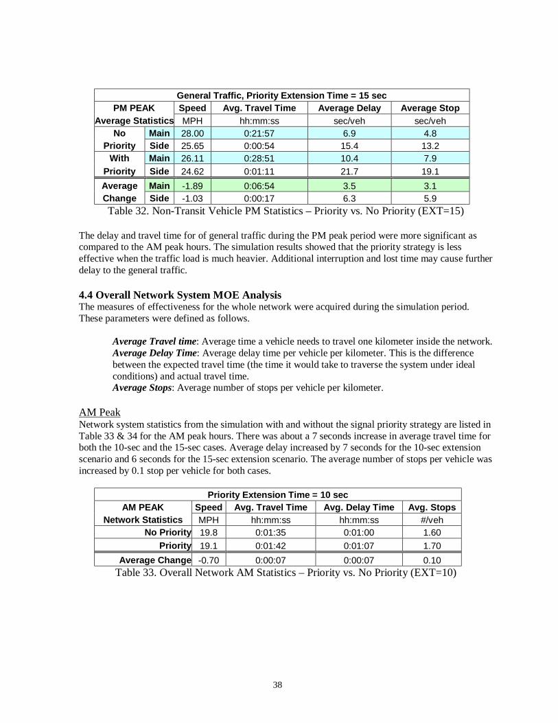
38

General Traffic, Priority Extension Time = 15 sec PM PEAK Speed Avg. Travel Time Average Delay Average Stop

Average Statistics MPH hh:mm:ss sec/veh sec/veh No Main 28.00 0:21:57 6.9 4.8

Priority Side 25.65 0:00:54 15.4 13.2 With Main 26.11 0:28:51 10.4 7.9

Priority Side 24.62 0:01:11 21.7 19.1 Average Main -1.89 0:06:54 3.5 3.1 Change Side -1.03 0:00:17 6.3 5.9 Table 32. Non-Transit Vehicle PM Statistics – Priority vs. No Priority (EXT=15)

The delay and travel time for of general traffic during the PM peak period were more significant as compared to the AM peak hours. The simulation results showed that the priority strategy is less effective when the traffic load is much heavier. Additional interruption and lost time may cause further delay to the general traffic. 4.4 Overall Network System MOE Analysis The measures of effectiveness for the whole network were acquired during the simulation period. These parameters were defined as follows.

Average Travel time: Average time a vehicle needs to travel one kilometer inside the network. Average Delay Time: Average delay time per vehicle per kilometer. This is the difference between the expected travel time (the time it would take to traverse the system under ideal conditions) and actual travel time. Average Stops: Average number of stops per vehicle per kilometer.

AM Peak Network system statistics from the simulation with and without the signal priority strategy are listed in Table 33 & 34 for the AM peak hours. There was about a 7 seconds increase in average travel time for both the 10-sec and the 15-sec cases. Average delay increased by 7 seconds for the 10-sec extension scenario and 6 seconds for the 15-sec extension scenario. The average number of stops per vehicle was increased by 0.1 stop per vehicle for both cases.

Priority Extension Time = 10 sec

AM PEAK Speed Avg. Travel Time Avg. Delay Time Avg. Stops Network Statistics MPH hh:mm:ss hh:mm:ss #/veh

No Priority 19.8 0:01:35 0:01:00 1.60 Priority 19.1 0:01:42 0:01:07 1.70

Average Change -0.70 0:00:07 0:00:07 0.10 Table 33. Overall Network AM Statistics – Priority vs. No Priority (EXT=10)

39

Overall Network System, Priority Extension Time = 15 sec

AM PEAK Speed Avg. Travel Time Avg. Delay Time Avg. Stops Network Statistics MPH hh:mm:ss hh:mm:ss #/veh

No Priority 19.8 0:01:35 0:01:00 1.60 Priority 19.1 0:01:42 0:01:06 1.70

Average Change -0.70 0:00:07 0:00:06 0.10 Table 34. Overall Network AM Statistics – Priority vs. No Priority (EXT=15)

PM Peak As a result of heavier traffic flow during the PM peak hours, the overall network statistics from the simulation with and without signal priority strategy generated longer delay and more vehicle stops. As listed in Table 35, the travel time during the PM period was increased by 22 seconds per kilometer when providing signal priority. Average delay was increased by 23 seconds while average stops increased by 0.6 stop per vehicle with the priority strategy.

Overall Network System, Priority Extension Time = 15 sec PM PEAK Speed Avg. Travel Time Avg. Delay Time Avg. Stops

Network Statistics MPH hh:mm:ss hh:mm:ss #/veh No Priority 18.1 0:01:55 0:01:19 2.00

Priority 16.0 0:02:17 0:01:42 2.60 Average Change -2.10 0:00:22 0:00:23 0.60

Table 35. Overall Network PM Statistics – Priority vs. No Priority (EXT=15) 4.5 Potential Saving of Bus Operation Bus cycle time is the number of minutes needed to make a round trip on the route, including layover or recovery time. Minimum layover or recovery time, recommended by Transit Cooperative Research Program (TCRP) Report 30, Transit Scheduling: Basic and Advanced Manuals [43], is 10% of the bus round trip time. Based on collected bus delay time at intersections (Table 8), we assume the following condition for bus route #2 as an example.

Bus route round trip time is 35 minutes per trip x 2 = 70 minutes, Average bus headway is about 15 minutes, and Excess layover time is 10 minutes (driver breaks etc.)

The total bus operation cycle time can be calculated as 70 x 1.10 + 10 = 87 minutes, and using the formula, Cycle time / Desired Headway = # Vehicles, 87 / 15 = 5.8 vehicles were needed for bus operation without signal priority. If we offer signal priority strategy that provides on average a 10% bus travel time saving, the total bus operation cycle time can be calculated as 70 x 90% x 1.10 + 10 = 79.3 minutes. Therefore, 79.3 / 15 = 5.3 vehicles would be required for bus operation using the signal priority strategy. Comparing the number of buses required for operation with and without signal priority, we could potentially save 0.5 buses of operation cost per bus route with signal priority.

40

5. FUTURE WORK We would like to investigate the 800 MHz radios and WLAN (Wireless Local Area Networks) systems already equipped on the bus. A voice radio on the bus is linked to a regional 800MHz digital voice communication system. Metro Transit Control Center uses another analog 800 MHz radio to poll bus GPS data every minute. In addition, each bus has a wireless communication system that is used to download/upload files between the central server and the bus computer when the bus is within proximity of the bus garage. We would like to investigate the possibility of integrating a signal priority strategy using one of the existing communication systems on the bus with the traffic controller. We also plan to develop a prototype system to validate the bus signal priority algorithm using wireless communication technology in a second phase of this study. We also would like to work with Metro Transit and City of Minneapolis to discuss the potential opportunity of bus signal priority deployment. Metro Transit is planning the Northwest Corridor (Bottineau Corridor) project so as to include a bus way that will offer high-quality transit service from downtown Minneapolis through Crystal, Brooklyn Park, Maple Grove and Rogers (http://www.metrotransit.org/improvingTransit/northwestCorridor.asp). In this project, bus signal priority will be considered in order to improve bus travel time and reduce bus delay at signalized intersections. Transit Signal Priority conceptual design along Bottineau Corridor is currently being investigated by SEH Inc. (http://www.sehinc.com/). The vision of the VII (Vehicle Infrastructure Integration, http://www.its.dot.gov/vii/index.htm) is to deploy a nationwide network that enables communications between vehicles and roadside infrastructure for various transportation operations and applications. Signal priority requests for transit or emergency vehicles can potentially be sent to the signal controller through the vehicle-to-infrastructure communication architecture described in VII. Communication with the roadside unit (e.g., traffic controller) for signal priority may be established using the existing 802.11x WLAN on the bus or the DSRC (Dedicated Short Range Communication) 802.11p protocol currently under development for wireless access to and from the vehicular environment. Work in next phase will concentrate first on the more readily available protocols. However the system will be designed so that it can be ported to the new 802.11p protocol when it becomes more readily available.

A Technical Advisory Panel (TAP) meeting was held at Metro Transit on April 20, 2006. Based on feedback from TAP review, we will further investigate any impact on transit vehicles by disabling signal priority at intersections (e.g. Nicollet and Cedar) that resulted in increase of intersection travel time and delay with signal priority strategy.

Finally as mentioned earlier, transit vehicles could potentially be used as probes for determining traffic speeds and travel times along freeways and major arterials [4]. Real-time traffic data could then be transmitted wirelessly to a regional TMC to adjust the intersection signal or ramp metering timing accordingly.

41

6. SUMMARY Transit Signal Priority (TSP) for transit has been proposed as an efficient way to improve transit travel & operation. Bus signal priority has been implemented in several US cities as well as in Europe. Various technologies have been deployed for bus signal priority using Opticom™ (St. Cloud) [5], Loopcom (Los Angeles), and RF tag (Seattle, King County) [6]. Current signal priority strategies implemented in various US cities mainly utilize sensors to detector buses at fixed or preset distances from intersections. Signal priority is usually granted after a preprogrammed time offset after detection. Engineers have to adjust the detector location, sensor line of sight or timing offset for each intersection to improve its effectiveness. These TSP strategies do not consider bus speed and its distance from intersection when determining the appropriate timing to provide signal priority.

A GPS/AVL-based adaptive signal priority strategy was developed to test the effectiveness on an arterial corridor through traffic simulation. This study took advantage of the GPS/AVL system already equipped on the buses in Minneapolis and developed an adaptive signal priority strategy that could consider the bus’s timeliness with respect to its schedule, its number of passengers, location and speed. Buses communicate with intersection signal controllers using wireless technology to request signal priority. Bus route #2 in Minneapolis was identified and investigated for providing bus signal priority. A simulation model of traffic conditions along the Franklin Corridor from Dupont to 27th Avenue (total of 22 signalized intersections) was created using the AIMSUN micro-simulation package (http://www.aimsun.com/). Signalized intersection traffic data and timing plans were obtained from City of Minneapolis. Traffic volumes and turning movements at un-signalized intersections were collected manually using JAMAR (http://www.jamartech.com/) hand-held traffic counter. Bus schedule and passenger arrivals were modeled using data collected by Metro Transit. The arterial network was then balanced and calibrated to provide a baseline model for priority strategy analysis.

The priority strategy was developed, implemented using C++ programming language and integrated with the simulator through the AIMSUN API interface. At each simulation step, bus location and its distance corresponding to the next bus stop and signalized intersection were calculated to determine nearside or far side bus stop scenario.

Simulation results indicated a 12%-15% reduction in bus travel time during AM peak hours (7AM-9AM) and 4-11% reduction during PM peak hours (4PM-6PM) could be achieved by providing signal priority for buses. Average bus delay time was reduced in the range of 16%-20% and 5%-14% during AM and PM peak periods, respectively. The signal priority strategy caused increases of travel time for non-transit vehicles of about 6 seconds per vehicle during AM peak and 22 seconds in the PM peak periods. The average number of non-transit vehicle stops increased from 1.6 stop/veh to 1.7 stop/veh during AM peak hours and from 2.0 stop/veh to 2.4 stop/veh during PM peak period.

42

REFERENCES [1] An Overview of Transit Signal Priority, (Advanced Traffic Management Systems Committee and

Advanced Public Transportation Systems Committee of the ITS America, 2002).

[2] Collura, J., Rakha, H., and Gifford, J., Guidelines for the Planning and Development of Emergency Vehicle Preemption and Transit Priority Strategies, (Virginia Tech Transportation Institute and George Mason University School of Public Policy, 2003).

[3] 3M™ Opticom™ Priority Control System, (Internet) http://www.3m.com/its (cited January 2005)

[4] F.W. Cathey and D.J. Dailey, “Transit Vehicles as Traffic Probe Sensors”, Transportation Research Record 1804, #02-2228

[5] St. Cloud Metropolitan Transit Commission Transit Priority Evaluation Report, Final Report, (St. Cloud, MN, Nov. 2000).

[6] An Evaluation of Transit Signal Priority on Aurora Avenue North, (Transit Speed and Reliability Program, King County Department of Transportation, Sep. 2002).

[7] 3M™ Opticom™ GPS Priority Control System, (Internet) http://www.3m.com/us/safety/tcm/ (cited January 2005)

[8] Split Cycle Offset Optimisation Technique (Internet) www.scoot-utc.com/SCOOTFacilities/busprior.htm, (cited September 2004)

[9] Liu, H., Skabardonis, A., Zhang, W.B., “A Dynamic Model For Adaptive Bus Signal Priority”, Transportation Research Board 82nd Annual Meeting, (Washington DC, January 2003).

[10] Kim, W. and Rilett, L.R., “An Improved Transit Signal Priority System for Networks With Nearside Bus Stops”, Transportation Research Board 84th Annual Meeting, (Washington, DC, January 2005).

[11] Bretherton, R.D., Hounsell, N.B., and Radia, B., “Public Transport Priority in SCOOT”, Proceedings of the 3rd Annual World Congress on ITS Systems, (Orlando, FL, Oct. 14-18, 1996).

[12] McLeod, F. and Hounsell, N., “Bus Priority at Traffic Signals – Evaluating Strategy Options”, Journal of Public Transportation, V6, No.3, (2003).

[13] Furth, P.G. and Mueller, T., “Conditional Bus Priority at Signalized Intersections”, 79th Annual Meeting of the Transportation Research Board, (Washington DC, 2000).

[14] Mirchandani, P.B. & Lucas, D.E., “Integrated Transit Priority and Rail/Emergency Preemption in Real-Time Traffic Adaptive Signal Control”, Journal of Intelligent Transportation Systems, Vol. 8 Issue 2, p101-115, (April 2004).

[15] Mirchandani, P.B. & Head, K.L., “A real-time traffic signal control system: Architecture, algorithms and analysis”, Transportation Research Record Part C, 9, 415-432, (2001).

[16] Lewis, V., Bus Priority Study, (Tualatin Valley Highway, Tri-Met, Portland, OR, 1996).

[17] Kloos, W.C., Danaher, A.R. and Hunter-Zaworski, K.M., “Bus Priority at Traffic Signals in Portland: The Powell Boulevard Pilot Project”, ITE Compendium of Technical Papers, (1994).

[18] King County Department of Transportation and City of Seattle Transportation, Transit Signal Priority System Assessment Study: Rainier Avenue South Field Evaluation Draft Report, (Seattle, WA, 2000).

[19] Illinois Department of Transportation and Civiltech Engineering, Inc., The Cermak Road Bus Priority Project Final Report, (Chicago, IL, 1998).

[20] Skehan, S., “Transit Signal Priority For Metro Rapid Bus in Los Angeles”, ITS America Transit Signal Priority Workshop, (Tuscon, AZ, April 2003).

[21] Pierce Transit. TSP Implementation Report. Prepared by DKS Associates. (Takoma, WA), (Internet) http://www.piercetransit.org/tsp.htm, (cited April 2003).

43

[22] Boje, B.F. and Nookala, M. “Signal Priority for Buses: An Operational Test at Louisiana Avenue, Minneapolis.” Compendium of Technical Papers for the 66th ITE Annual Meeting, (Washington, DC, 1996, pp. 309-313).

[23] An Overview of Transit Signal Priority, (Advanced Traffic Management Systems Committee and Advanced Public Transportation Systems Committee of the ITS America, revised and updated 2004).

[24] Synchro, traffic signal coordination software by Trafficware Corporation, (Albany, CA). (Internet) http://www.trafficware.com/ (cited January 2005).

[25] JAMAR Hand-held traffic data collector, DB-400, (Horsham, PA). (Internet) http://www.trafficcounter.com/ (cited June 2005).

[26] Minnesota Department of Transportation, MnCON, (Internet) http://rocky.dot.state.mn.us/Inside_LM/LIS/MnCON/mncon.html, version 2.4.1, (cited July 19, 2004).

[27] Ericksen, D.E., “NAD83: What is it and Why You Should Care”, 1994 SBE National Convention and World Media Expo, (Los Angeles, CA 1994).

[28] Transit Cooperative Research Program (TCRP) Report 100: Transit Capacity and Quality Service Manual, 2nd Edition – Part 4: Bus Transit Capacity, Chapter 1, Bus Capacity Fundamentals, pp. 4-3 ~ 4-9. (Internet) http://trb.org/news/blurb_detail.asp?id=2326 (cited June 2005).

[29] Scheel, W. and J.E. Foote, “Bus Operation in Single Lane Platoons and Their Ventilation Needs for Operation in Tunnels,” Research Publication GMR-808, General Motors Research Laboratories, (Warren, MI, 1962).

[30] St. Jacques, Kevin and Herbert S. Levinson, "Operational Analysis of Bus Lanes on Arterials," TCRP Report 26, Transportation Research Board, (Washington, DC, 1997).

[31] Transport Simulation Systems (TSS), AIMSUN Version 4.1 User’s Manual, (Barcelona, Spain, Mar. 2002).

[32] Transport Simulation Systems (TSS), GETRAM Extensions Version 4.1 User’s Manual, (Barcelona, Spain, Mar. 2002).

[33] Hourdakis, J., Michalopoulos, P. and J. Kottommannil. “Practical procedure for calibrating microscopic traffic simulation models” Transportation Research Record 1852: pp. 130-139, (Washington DC, 2003).

[34] Xin, W.P., “User Manual for Arterial Intersection Data Balancing Tool, ArtBaT”, (Department of Civil Engineering, University of Minnesota, 2005).

[35] Federal Highway Administration, Traffic Analysis Toolbox Volume III: Guidelines for Applying Traffic Microsimulation Modeling Software, FHWA-HRT-04-040, (McLean, VA, July 2004).

[36] Theil, H., Applied Economic Forecasting, North-Holland Publishers, (Amsterdam, 1966).

[37] Pindyck R.S. and Rubinfeld D.L., “Econometric models and economic forecasts”, 4th edition, Irwin McGraw-Hill, (Boston MA, 1997).

[38] Reinhoudt, Edwin M., and S. A. Velastin, “A dynamic predicting algorithm for estimating bus arrival time”, Proceedings of the 8th IFAC/IFIP/IFORS Symposium, Vol. 3., pp.1295-8, (Chania, Greece, 16-18 June 1997).

[39] D.J. Dailey, Z.R. Wall, S.D. Maclean and F.W. Cathey, “An Algorithm and Implementation to Predict the Arrival of Transit Vehicles”, ITSC, (2000), (Internet) http://www.its.washington.edu/pubs/itsc_2000.pdf (cited May 2005).

[40] Shalaby A. and Farhan A., “Prediction Model of Bus Arrival and Departure Times Using AVL and APC Data”, Journal of Public Transportation, Vol. 7, No. 1, (2004).

[41] Eagle Traffic Control Systems, SEPAC Actuated Signal Control Software, User’s manual, (Feb. 2002).

[42] Eagle EPAC M50 Traffic Control Unit, (Internet) http://www.itssiemens.com/en/t_nav282.html (cited July 2005).

44

[43] Pine, R., Niemeyer, J. and Chisholm, R., “TCRP Report 30, Transit Scheduling: Basic and Advanced Manuals”, TRB National Research Council, National Academy Press, (Washington, DC 1998), pp.18-21.

[44] Li, M., Yin, Y., Zhou, K., Zhang, W.B., Liu, H., and Tan, C.W., “Adaptive Transit Signal Priority on Actuated Signalized Corridors”, Transportation Research Board 84nd Annual Meeting, (Washington DC, January 2005).

[45] P B. Mirchandani, A. Knyazyan, K.L. Head, and W. Wu, “An Approach Towards the Integration of Bus Priority, Traffic Adaptive Signal Control, and Bus Information/Scheduling Systems,” Computer-Aided Scheduling of Public Transport, (Springer-Verlag, Germany, 2001) , 319-334,

[46] Dion F. and Rakha H., “Integration of Transit Signal Priority Within Adaptive Traffic Control Systems”, Transportation Research Board 84nd Annual Meeting, (Washington DC, January 2005).

[47] Crout D.T., “Evaluation of Transit Signal Priority at the Tri-County Metropolitan Transportation District of Oregon (TriMet)”, Proceedings of the 12th Annual World Congress on ITS Systems, (San Francisco, CA, Nov. 6-10, 2005).

APPENDIX A

Intersection Signal Timing Plans

A-1

The splits and offset in the original signal timing obtained from the City of Minneapolis

Public Works department was expressed in percentage of cycle length. They were converted in seconds as listed below for the timing plan in the simulation model. The phase numbers were assigned using the NEMA phasing convention as shown in Figure A.1.

Figure A.1 NEMA Phasing Assignment [22]

A.1. AM Peak Signal Timing Plan: AM-PEAK (06:00-08:45)

ID Intersection Name Cycle Split (sec) Offset (sec) 1 2 3 4 5 6 7 8 (sec)

298 Dupont Ave S & W Franklin Ave 90 63.0 27.0 0.0 0.0 0.0 0.0 0.0 0.0 78.30 297 W Franklin Ave & Hennepin Ave 90 0.0 36.0 16.2 37.8 0.0 36.0 16.2 37.8 48.60 381 W Franklin Ave & Lyndale Ave S 90 34.2 39.6 16.2 0.0 0.0 0.0 0.0 0.0 36.00 49 Blaisdell Ave & W Franklin Ave 90 0.0 54.9 0.0 35.1 0.0 0.0 0.0 0.0 14.40 98 Franklin Ave & Nicollet Ave 90 0.0 32.4 0.0 57.6 0.0 0.0 0.0 0.0 77.40 833 E Franklin Ave & 1st Ave S 90 0.0 51.3 0.0 38.7 0.0 0.0 0.0 0.0 23.40 236 E Franklin Ave & 3rd Ave S 90 65.7 24.3 0.0 0.0 0.0 0.0 0.0 0.0 43.20 254 Clinton Ave & E Franklin 90 0.0 60.3 0.0 29.7 0.0 0.0 0.0 0.0 43.20 161 E Franklin Ave & 4th Ave S 90 67.5 22.5 0.0 0.0 0.0 0.0 0.0 0.0 48.60 347 E Franklin Ave & 5th Ave S 90 13.5 49.5 0.0 27.0 0.0 0.0 0.0 0.0 47.70 187 E Franklin Ave & Portland Ave 90 54.0 36.0 0.0 0.0 0.0 0.0 0.0 0.0 39.60 256 E Franklin Ave & Park Ave 90 28.8 61.2 0.0 0.0 0.0 0.0 0.0 0.0 36.00 489 Chicago Ave & E Franklin Ave 90 13.5 47.7 0.0 28.8 13.5 47.7 0.0 28.8 39.60 491 E Franklin Ave & 11th Ave S 90 13.5 46.8 0.0 29.7 13.5 46.8 0.0 29.7 89.10 492 E Franklin Ave & 13th Ave S 90 13.5 48.6 0.0 27.9 0.0 0.0 0.0 0.0 87.30 869 E Franklin Ave & 15th Ave S 90 13.5 49.5 0.0 27.0 0.0 0.0 0.0 0.0 24.30 845 Bloomington Ave & E Franklin Ave 90 13.5 50.4 0.0 26.1 0.0 0.0 0.0 0.0 37.80 210 E Franklin Ave & 17 Ave S 110 13.2 27.5 19.8 49.5 0.0 40.7 0.0 69.3 0.00 203 Cedar Ave & E Franklin Ave 90 36.0 11.7 42.3 0.0 0.0 0.0 0.0 0.0 57.60 206 E Franklin Ave & Minnehaha Ave 90 45.0 45.0 0.0 0.0 0.0 0.0 0.0 0.0 55.80 938 E Franklin Ave & 22nd Ave S 90 54.0 36.0 0.0 0.0 0.0 0.0 0.0 0.0 62.10 44 E Franklin Ave & 26th Ave S 90 54.0 36.0 0.0 0.0 0.0 0.0 0.0 0.0 33.30

A-2

A.2. PM Peak Signal Timing Plan: PM-PEAK (15:00-18:30)

ID Intersection Name Cycle Split (sec) Offset (sec) 1 2 3 4 5 6 7 8 (sec)

298 Dupont Ave S & W Franklin Ave 120 92.4 27.6 0.0 0.0 0.0 0.0 0.0 0.0 61.20 297 W Franklin Ave & Hennepin Ave 120 0.0 66.0 16.8 37.2 0.0 66.0 16.8 37.2 61.20 381 W Franklin Ave & Lyndale Ave S 90 34.2 39.6 16.2 0.0 0.0 0.0 0.0 0.0 63.90 49 Blaisdell Ave & W Franklin Ave 90 0.0 43.2 0.0 46.8 0.0 0.0 0.0 0.0 84.60 98 Franklin Ave & Nicollet Ave 90 0.0 26.1 0.0 63.9 0.0 0.0 0.0 0.0 55.80 833 E Franklin Ave & 1st Ave S 90 0.0 63.0 0.0 27.0 0.0 0.0 0.0 0.0 81.90 236 E Franklin Ave & 3rd Ave S 90 61.2 28.8 0.0 0.0 0.0 0.0 0.0 0.0 10.80 254 Clinton Ave & E Franklin 90 0.0 60.3 0.0 29.7 0.0 0.0 0.0 0.0 14.40 161 E Franklin Ave & 4th Ave S 90 67.5 22.5 0.0 0.0 0.0 0.0 0.0 0.0 9.90 347 E Franklin Ave & 5th Ave S 90 18.0 41.4 0.0 30.6 0.0 0.0 0.0 0.0 25.20 187 E Franklin Ave & Portland Ave 90 45.9 44.1 0.0 0.0 0.0 0.0 0.0 0.0 15.30 256 E Franklin Ave & Park Ave 90 36.0 54.0 0.0 0.0 0.0 0.0 0.0 0.0 8.10 489 Chicago Ave & E Franklin Ave 90 13.5 47.7 0.0 28.8 13.5 47.7 0.0 28.8 12.60 491 E Franklin Ave & 11th Ave S 90 13.5 46.8 0.0 29.7 13.5 46.8 0.0 29.7 44.10 492 E Franklin Ave & 13th Ave S 90 13.5 48.6 0.0 27.9 0.0 0.0 0.0 0.0 45.00 869 E Franklin Ave & 15th Ave S 90 13.5 49.5 0.0 27.0 0.0 0.0 0.0 0.0 61.20 845 Bloomington Ave & E Franklin Ave 90 13.5 50.4 0.0 26.1 0.0 0.0 0.0 0.0 49.50 210 E Franklin Ave & 17 Ave S 110 13.2 27.5 19.8 49.5 0.0 40.7 0.0 69.3 0.00 203 Cedar Ave & E Franklin Ave 90 42.3 11.7 36.0 0.0 0.0 0.0 0.0 0.0 21.60 206 E Franklin Ave & Minnehaha Ave 90 45.0 45.0 0.0 0.0 0.0 0.0 0.0 0.0 18.90 938 E Franklin Ave & 22nd Ave S 90 54.0 36.0 0.0 0.0 0.0 0.0 0.0 0.0 18.90 44 E Franklin Ave & 26th Ave S 90 54.0 36.0 0.0 0.0 0.0 0.0 0.0 0.0 60.30

A-3

A.3. Off Peak Signal Timing Plan:

OFF-PEAK ID Intersection Name Cycle Split (sec) Offset (sec) 1 2 3 4 5 6 7 8 (sec)

298 Dupont Ave S & W Franklin Ave 90 50.4 39.6 0.0 0.0 0.0 0.0 0.0 0.0 24.30 297 W Franklin Ave & Hennepin Ave 65 0.0 26.0 11.7 27.3 0.0 26.0 11.7 27.3 41.60 381 W Franklin Ave & Lyndale Ave S 90 34.2 39.6 16.2 0.0 0.0 0.0 0.0 0.0 39.60 49 Blaisdell Ave & W Franklin Ave 70 0.0 35.7 0.0 34.3 0.0 0.0 0.0 0.0 21.00 98 Franklin Ave & Nicollet Ave 70 0.0 32.9 0.0 37.1 0.0 0.0 0.0 0.0 58.10 833 E Franklin Ave & 1st Ave S 70 0.0 42.0 0.0 28.0 0.0 0.0 0.0 0.0 18.20 236 E Franklin Ave & 3rd Ave S 70 42.7 27.3 0.0 0.0 0.0 0.0 0.0 0.0 56.70 254 Clinton Ave & E Franklin 70 0.0 40.6 0.0 29.4 0.0 0.0 0.0 0.0 53.20 161 E Franklin Ave & 4th Ave S 70 47.6 22.4 0.0 0.0 0.0 0.0 0.0 0.0 51.80 347 E Franklin Ave & 5th Ave S 70 13.3 29.4 0.0 27.3 0.0 0.0 0.0 0.0 32.20 187 E Franklin Ave & Portland Ave 70 35.0 35.0 0.0 0.0 0.0 0.0 0.0 0.0 25.20 256 E Franklin Ave & Park Ave 70 35.0 35.0 0.0 0.0 0.0 0.0 0.0 0.0 21.70 489 Chicago Ave & E Franklin Ave 70 13.3 28.7 0.0 28.0 13.3 28.7 0.0 28.0 1.40 491 E Franklin Ave & 11th Ave S 70 13.3 27.3 0.0 29.4 13.3 27.3 0.0 29.4 32.90 492 E Franklin Ave & 13th Ave S 70 13.3 29.4 0.0 27.3 0.0 0.0 0.0 0.0 32.20 869 E Franklin Ave & 15th Ave S 70 13.3 29.4 0.0 27.3 0.0 0.0 0.0 0.0 65.10 845 Bloomington Ave & E Franklin Ave 70 13.3 30.1 0.0 26.6 0.0 0.0 0.0 0.0 58.10 210 E Franklin Ave & 17 Ave S 110 13.2 27.5 19.8 49.5 0.0 40.7 0.0 69.3 0.00 203 Cedar Ave & E Franklin Ave 70 30.8 11.2 28.0 0.0 0.0 0.0 0.0 0.0 6.30 206 E Franklin Ave & Minnehaha Ave 70 35.0 35.0 0.0 0.0 0.0 0.0 0.0 0.0 4.20 938 E Franklin Ave & 22nd Ave S 70 35.0 35.0 0.0 0.0 0.0 0.0 0.0 0.0 44.80 44 E Franklin Ave & 26th Ave S 70 37.8 32.2 0.0 0.0 0.0 0.0 0.0 0.0 4.20

APPENDIX B

Bus GPS Data and Conversion

B-1

B.1 Bus Stop Location Bus stop location data were obtained from Metro Transit in latitude/longitude format. Both east and westbound bus stops are listed as follows.

Rte Dir Stop Name Stop ID Lat Long M-2 E HENNEPIN AV & 22 ST W 1099 449610605 -932927756M-2 E DUPONT AV & FRANKLIN AV W 13340 449625591 -932930243M-2 E FRANKLIN AV W & HENNEPIN AV S 13337 449626554 -932911021M-2 E FRANKLIN AV W & LYNDALE AV S 13334 449626285 -932882723M-2 E FRANKLIN AV W & HARRIET AV 13333 449626531 -932856366M-2 E FRANKLIN AV W & PLEASANT AV 13330 449626576 -932830738M-2 E FRANKLIN AV W & BLAISDELL AV 13326 449626595 -932797746M-2 E FRANKLIN AV W & NICOLLET AV 13325 449626526 -932782031M-2 E FRANKLIN AV E & 1 AV S 40560 449626508 -932760666M-2 E FRANKLIN AV E & 3 AV S 13320 449626473 -932729708M-2 E FRANKLIN AV E & 4 AV S 13317 449626714 -932705195M-2 E FRANKLIN AV E & PORTLAND AV 13316 449626496 -932672270M-2 E FRANKLIN AV E & PARK AV 13313 449626513 -932645798M-2 E FRANKLIN AV E & CHICAGO AV 13312 449626519 -932627721M-2 E FRANKLIN AV E & 10 AV S 13310 449626496 -932598066M-2 E FRANKLIN AV E & 11 AV S 13306 449626628 -932576848M-2 E FRANKLIN AV E & 13 AV / 14 AV S 15664 449626600 -932565263M-2 E FRANKLIN AV E & BLOOMINGTON AV S 15668 449626823 -932525226M-2 E FRANKLIN AV E & 16 AV S 13283 449626841 -932512386M-2 E FRANKLIN AV E & FRANKLIN STATION 51532 449624086 -932471827M-2 E FRANKLIN AV E & CEDAR AV 13277 449625306 -932454093M-2 E FRANKLIN AV E & MINNEHAHA AV 13275 449626456 -932445561M-2 E FRANKLIN AV E & 22 AV S 13269 449627064 -932411081M-2 E FRANKLIN AV E & 24 AV S 13261 449627196 -932379281M-2 E FRANKLIN AV E & 25 AV S 13257 449627116 -932363388M-2 E 26 AV S & FRANKLIN AV E 13249 449630501 -932345173Table B.1 Route #2 Eastbound – Franklin Ave. Bus Stop coordinate (x107 degree)

B-2

Rte Dir Stop Name Stop ID Lat Long M-2 W 27 AV S & FRANKLIN AV E 13247 449629065 -932330571M-2 W FRANKLIN AV E & 26 AV S 13253 449627470 -932345810M-2 W FRANKLIN AV E & 24 AV S 13259 449627480 -932377470M-2 W FRANKLIN AV E & 23 AV S 13263 449627490 -932393410M-2 W FRANKLIN AV E & 22 AV S 13267 449627480 -932409300M-2 W FRANKLIN AV E & MINNEHAHA / CEDAR AV 13279 449627620 -932447080M-2 W FRANKLIN AV E & FRANKLIN STATION 51533 449627161 -932468556M-2 W FRANKLIN AV E & 16 AV S 41156 449628110 -932510850M-2 W FRANKLIN AV E & BLOOMINGTON AV S 15630 449628352 -932528271M-2 W FRANKLIN AV E & 13 AV S 13297 449628696 -932566078M-2 W FRANKLIN AV E & 11 AV S 13303 449628562 -932579165M-2 W FRANKLIN AV E & 10 AV S 13309 449628583 -932595206M-2 W FRANKLIN AV E & CHICAGO AV 13311 449628513 -932632386M-2 W FRANKLIN AV E & PARK AV 13314 449628348 -932649064M-2 W FRANKLIN AV E & PORTLAND AV 13315 449628268 -932674383M-2 W FRANKLIN AV E & CLINTON AV 13318 449628228 -932713373M-2 W FRANKLIN AV E & 3 AV S 13319 449628170 -932725743M-2 W FRANKLIN AV E & 1 AV S 13322 449628251 -932764023M-2 W FRANKLIN AV W & NICOLLET AV 13324 449628176 -932782483M-2 W FRANKLIN AV W & PILLSBURY AV 13328 449628164 -932807098M-2 W FRANKLIN AV W & HARRIET AV 13332 449628198 -932852636M-2 W FRANKLIN AV W & LYNDALE AV S 13335 449628176 -932886441M-2 W HENNEPIN AV & FRANKLIN AV W 1096 449624199 -932918338M-2 W HENNEPIN AV & FRANKLIN AV / 22 ST W 42883 449618940 -932920865M-2 W HENNEPIN AV & FRANKLIN / 22 ST 51581 449618998 -932921246Table B.2 Route #2 Westbound – Franklin Ave. Bus Stop coordinate (x107 degree)

B.2 Convert GPS Data to State Plane Coordinate System (SPCS) A Java program, as listed below, was developed to identify the per-minute bus GPS data collected while traveling on Franklin Ave and convert the lat-long projections into MN-S state plane coordinate.

/* * latlong2xy.java * * Read in Metro Transit bus GPS data/report file and convert lat-long data format * to NAD83 Minnesota South 2203 SPCS XY coordinate * * Created on August 18, 2005, 3:49 PM */ /* * @author Chen-Fu Liao */ import java.awt.geom.* ; import java.io.* ; public class latlong2xy { /** Creates a new instance of latlong2xy */ public latlong2xy() { }

public static void main(String[] args) { // TODO code application logic here String data_filename = args[0] ; String filepath = "" ; String out_filename = "" ; int num_rpts = 0 ; // num of report files String[] data_files = null ; System.out.println(data_filename) ; // read intersection filenames try { BufferedReader in = new BufferedReader(new FileReader(data_filename)) ; String str ; filepath = in.readLine() ; num_rpts = Integer.valueOf(in.readLine()).intValue() ; System.out.println(filepath + ", num_rpts = " + num_rpts ) ; data_files = new String[num_rpts] ; /* while ((str = in.readLine()) != null) { System.out.println(str) ; } */

B-3

for (int i=0; i<num_rpts; i++) { data_files[i] = in.readLine() ; //System.out.println(data_files[i]) ; } in.close() ; } catch (IOException e) { System.out.println("Error: " + e.toString()) ; } for (int i = 0; i<num_rpts; i++) { //num_rpts // read & process each gpa data file try { BufferedReader in = new BufferedReader(new FileReader(filepath+data_files[i])) ; out_filename = filepath + data_files[i] + ".csv" ; boolean exists = (new File(out_filename)).exists() ; if (exists) { // delete file boolean sucess = (new File(out_filename)).delete() ; } BufferedWriter out = new BufferedWriter(new FileWriter(out_filename, true)) ; out.write("latitude,longtitude,date,time,SPCS_X,SPCS_Y\n") ; String str ; String str_lat, str_long, str_date, str_time ; int line = 0, str_len = 0 ; double _lat, _long ; double _X, _Y ; while ((str = in.readLine()) != null) { line ++ ; str_len = str.length() ; if (line >=12 && str_len >515) { // string processing //System.out.println(str) ; //System.out.println(str.length()) ; str_lat = str.substring(112, 123) ; str_lat = str_lat.trim() ; str_long = str.substring(124, 135) ; str_long = str_long.trim() ; if (str_lat.length()>=9 && str_long.length()>=9) { _lat = Double.valueOf(str_lat).doubleValue()/10000000 ; _long = Double.valueOf(str_long).doubleValue()/10000000 ; //System.out.println(_lat + "," + _long) ; str_date = str.substring(490, 500) ; str_date = str_date.trim() ; str_time = str.substring(515, str_len) ; str_time = str_time.trim() ;

Point2D.Double lat_long = new Point2D.Double(_lat, _long) ; Point2D.Double spcs_xy = new Point2D.Double() ; spcs_xy = convert2XY(lat_long) ; _X = spcs_xy.getX() ; _Y = spcs_xy.getY() ; if ( (_X<860560) && (_X>855775) && (_Y<318388) && (_Y>318235)) { //System.out.println(str_lat + "," + str_long+","+ str_date + "," + str_time+","+_X+","+_Y) ; out.write(_lat + "," + _long+","+ str_date + "," + str_time+","+_X+","+_Y+"\n") ; } // if _X _Y } // if _length >=9 } // if line } // while out.close() ; in.close() ; } catch (IOException e) { System.out.println("Error: [" + data_files[i] + "]"+ e.toString()) ; } System.out.println( data_files[i] + " Done!") ; } // i System.out.println("Finished!") ; // System.out.println("X=" + spcs_xy.getX()+", Y="+spcs_xy.getY()) ; } public static Point2D.Double convert2XY(Point2D.Double myLatLong) { double sin_phi0, sin_phi ; double gamma, Ln1, Ln2, R, Q ; double DEG_2_RAD = Math.PI / 180.0 ; coord_const constants = new coord_const(2203) ; // NAD83 MN South zone Point2D.Double mySPCSxy = new Point2D.Double() ; sin_phi0 = Math.sin((constants.phi_zero*DEG_2_RAD)) ; gamma = (constants.lambda_zero+myLatLong.y)*sin_phi0 *DEG_2_RAD ; sin_phi = Math.sin(myLatLong.x*DEG_2_RAD) ; Ln1 = Math.log((1.0+sin_phi)/(1.0-sin_phi)) ; Ln2 = Math.log((1.0+constants.E*sin_phi)/(1.0-constants.E*sin_phi)) ; Q = 0.5*(Ln1-constants.E*Ln2) ; R = constants.K/Math.exp(Q*sin_phi0) ; mySPCSxy.x = (constants.E_zero+R*Math.sin(gamma)) ; mySPCSxy.y = (constants.Rb+constants.Nb-R*Math.cos(gamma)) ; return mySPCSxy ; } }

B-4

B.3 Bus Travel Time From Per-Minute GPS Data

Bus Travel Time (mm:ss) 8/23/2005 Bus ID 508 675 681 926 934

AM EB 21:32 17:10 17:26 19:41 17:00 PEAK WB 16:38 17:46 18:36 16:30 18:00

PM EB 16:47 18:15 n/a 21:45 18:44 PEAK WB 18:14 23:00 21:22 18:01 19:34

Table B.3 Bus Travel Time Calculated From GPS Data (8/23/05)

Bus Travel Time (mm:ss) 8/24/2005 Bus ID 507 508 622 675 843 846 849 926 934

AM EB 18:47 21:32 19:30 19:59 20:40 20:11 20:21 21:49 19:00 PEAK WB 17:07 17:44 17:17 17:46 16:50 17:04 18:44 16:30 18:00

PM EB 21:23 21:54 19:10 18:15 19:46 27:17 17:27 20:42 19:34 PEAK WB 18:15 19:14 21:45 23:00 23:44 18:29 n/a 18:03 18:44

Table B.4 Bus Travel Time Calculated From GPS Data (8/24/05)

APPENDIX C

Bus Passenger Count and Dwell Time Statistics

C-1

C.1 Passenger Boarding/Alighting Statistics Following data were average calculated from a 9-day passenger count data collection study during 2000 and 2001 by Metro Transit (4/20, 4/24, 4/25, 4/26, 4/27, 5/1, 5/2, 5/9 of year 2000, and 2/19/2001).

ROUTE 2 - Franklin Ave

EASTBOUND Passenger Boarding/Alighting Counts WEEKDAY AM Peak Boarding PM Peak Boarding AM Peak Alighting PM Peak Alighting Bus Stop AVG STDEV AVG STDEV AVG STDEV AVG STDEV

Dupont Ave. 2.00 1.73 0.00 0.00 0.00 0.00 0.00 0.00 Bryant Ave. S. 1.80 1.03 2.50 0.71 0.00 0.00 0.00 0.00 Aldrich Ave. S. 0.00 0.00 0.00 0.00 0.00 0.00 0.00 0.00 Lyndale Ave. S. 1.89 1.45 3.67 2.42 0.00 0.00 0.00 0.00 Harriet Ave. 1.67 1.21 1.00 0.00 0.00 0.00 0.00 0.00 Pleasant Ave. 1.50 0.76 0.00 0.00 0.00 0.00 1.00 0.00 Pillsbury Ave. 1.50 0.58 1.00 0.00 0.00 0.00 0.00 0.00 Blaisdell Ave. 1.00 0.00 0.00 0.00 0.00 0.00 0.00 0.00 Nicollet Ave. 4.55 2.11 8.50 5.18 1.25 0.50 1.33 0.52 1 Ave. S. 2.91 2.47 3.50 2.38 1.00 0.00 1.50 0.71 3 Ave. S. 4.22 2.28 2.67 1.51 1.25 0.50 1.00 0.00 Clinton Ave. S. 1.60 1.34 1.00 0.00 0.00 0.00 1.00 0.00 4 Ave. S. 1.33 0.58 3.33 4.04 0.00 0.00 1.33 0.58 Portland Ave. 1.88 1.46 1.33 0.58 1.00 0.00 3.33 4.04 Park Ave. 1.60 0.89 2.00 0.00 2.00 1.41 1.00 0.00 Chicago Ave. 2.67 1.03 2.86 2.41 2.55 1.57 2.86 2.41 10 Ave. S. 1.40 0.55 1.00 0.00 1.00 0.00 1.00 0.00 11 Ave. S. 1.43 0.79 2.33 2.31 1.00 0.00 3.67 3.79 14 Ave. S. 1.50 0.84 2.00 0.71 1.67 1.15 3.67 1.51 15 Ave. S. 1.50 0.71 2.00 0.00 1.00 0.00 2.00 0.00 Bloomington Ave 1.43 0.79 1.67 0.52 1.67 0.71 1.60 0.89 16 Ave. S. 1.00 0.00 1.00 0.00 1.00 0.00 1.67 0.58 Cedar Ave. 0.00 0.00 1.00 0.00 2.83 1.17 2.00 0.82 Minnehaha Ave. 1.33 0.58 1.67 0.58 1.00 0.00 2.33 1.53 21 Ave. S. 1.67 0.58 0.00 0.00 1.00 0.00 1.33 0.58 22 Ave. S. 1.67 0.82 8.00 0.00 2.00 0.00 3.00 2.16 23 Ave. S. 1.00 0.00 0.00 0.00 0.00 0.00 2.00 0.00 24 Ave. S. 2.50 1.73 1.00 0.00 1.00 0.00 0.00 0.00 25 Ave. S. 2.00 1.41 3.00 0.00 1.00 0.00 5.00 0.00 26 Ave. S. 3.25 2.22 1.20 0.45 3.38 0.74 1.86 1.07

Table C.1 Eastbound AM & PM Peak Bus Passenger Counts

C-2

ROUTE 2 - Franklin Ave

WESTBOUND Passenger Boarding/Alighting Counts WEEKDAY AM Peak Boarding PM Peak Boarding AM Peak Alighting PM Peak Alighting Bus Stop AVG STDEV AVG STDEV AVG STDEV AVG STDEV

26 Ave. S. 3.67 2.34 3.00 1.73 1.00 0.00 1.00 0.00 25 Ave. S. 1.33 0.58 1.00 0.00 0.00 0.00 1.00 0.00 24 Ave. S. 1.17 0.41 1.33 0.58 4.00 0.00 1.75 1.50 23 Ave. S. 1.60 0.55 1.00 0.00 1.00 0.00 1.50 1.00 22 Ave. S. 3.00 1.83 2.00 1.00 1.00 0.00 1.00 0.00 21 Ave. S. 2.00 1.41 1.00 0.00 1.00 0.00 1.29 0.76 Minnehaha 1.75 1.16 4.38 3.70 2.00 1.00 1.00 0.00 Bloomington Ave 1.50 0.58 1.00 0.00 2.25 1.58 1.40 0.55 15 Ave. S. 2.40 1.52 1.50 0.71 2.00 1.41 1.50 0.58 14 Ave. S. 1.56 1.33 2.86 2.04 1.00 0.00 2.00 1.55 11 Ave. S. 2.00 1.41 2.00 1.41 1.25 0.50 1.60 1.34 10 Ave. S. 4.00 0.00 1.00 0.00 1.00 0.00 1.33 0.58 Chicago Ave. 1.75 1.16 3.25 2.38 3.10 1.85 5.33 3.87 Park Ave. 1.75 0.96 3.00 2.12 1.33 0.58 1.25 0.50 Portland Ave. 1.00 0.00 1.50 0.71 2.00 1.41 1.67 0.58 Clinton Ave. 1.17 0.41 2.67 2.89 2.00 0.00 4.40 2.30 3 Ave. S. 1.75 0.96 1.00 0.00 1.67 0.82 3.38 2.26 Stevens Ave. 1.25 0.50 0.00 0.00 1.00 0.00 1.50 1.00 1 Ave. S. 0.00 0.00 1.00 0.00 2.00 1.00 2.20 1.10 Nicollet Ave. 1.33 0.58 1.33 0.58 6.70 5.79 8.44 4.50 LaSalle Ave. 0.00 0.00 1.00 0.00 1.50 0.71 1.50 0.71 Pillsbury Ave. 0.00 0.00 0.00 0.00 1.33 0.58 1.67 1.15 Pleasant Ave. 1.00 0.00 0.00 0.00 1.00 0.00 1.50 0.53 Harriet Ave. 0.00 0.00 0.00 0.00 0.00 0.00 1.00 0.00 Lyndale Ave. S. 0.00 0.00 0.00 0.00 1.83 0.75 3.13 1.81 Aldrich Ave. S. 0.00 0.00 0.00 0.00 1.00 0.00 1.00 0.00 Hennepin Ave. E. 0.00 0.00 0.00 0.00 3.22 1.48 2.00 0.93

Table C.2 Westbound AM & PM Peak Bus Passenger Counts

C-3

C.2 Bus Dwell Time Statistics Based on Passenger Counts

Eastbound AM PM Bus Stop Bus Dwell Time (s) Bus Dwell Time (s)

ID Name DWELL STDEV DWELL STDEV 1006 Franklin Ave. W. 3.10 1.91 2.50 0.00 3337 Bryant Ave. S. 4.30 1.14 3.00 0.78 3334 Lyndale Ave. S. 4.20 1.60 4.70 2.66 3333 Harriet Ave. 3.50 1.33 2.60 0.00 3330 Pleasant Ave. 3.70 0.83 2.59 0.00 1004 Pillsbury Ave. 3.10 0.64 2.70 0.00 3326 Blaisdell Ave. 2.80 0.00 2.50 0.00 3325 Nicollet Ave. 7.91 2.78 10.02 6.17 560 1 Ave. S. 5.78 2.71 4.17 3.25 3320 3 Ave. S. 6.71 2.96 4.19 1.66 3317 4 Ave. S. 2.90 0.64 3.86 4.97 3316 Portland Ave. 4.16 1.60 3.80 4.27 3313 Park Ave. 3.95 2.26 2.79 0.00 3312 Chicago Ave. 6.39 2.55 6.30 4.82 3310 10 Ave. S. 3.53 0.60 2.69 0.00 3306 11 Ave. S. 3.58 0.87 4.19 5.95 5664 14 Ave. S. 3.81 1.96 5.48 2.13 1008 15 Ave. S. 2.96 0.78 3.06 0.00 5668 Bloomington Ave 4.73 1.50 4.22 1.37 3283 16 Ave. S. 2.88 0.00 3.05 0.52 1532 17 Ave. S.* 2.00 1.00 2.00 1.00 1002 LRT Cedar/Riverside* 4.00 1.00 4.00 1.00 3277 Cedar Ave. 3.89 1.05 3.42 0.73 3275 Minnehaha Ave. 3.31 0.64 3.63 2.01 3269 22 Ave. S. 3.66 0.90 4.38 1.94 3261 24 Ave. S. 3.66 1.91 2.70 0.00 3257 25 Ave. S. 2.98 1.56 3.25 0.00 3249 Franklin Ave. E. 6.01 3.11 4.27 1.45

*Insufficient data. Use average value. Table C.3 Eastbound AM & PM Peak Bus Dwell Time

C-4

Westbound AM PM Bus Stop Bus Dwell Time (s) Bus Dwell Time (s)

ID Name DWELL STDEV DWELL STDEV 3253 26 Ave. S. 5.01 2.57 5.17 1.91 3259 24 Ave. S. 3.63 0.45 3.57 1.99 3263 23 Ave. S. 3.47 0.60 3.26 0.90 3267 22 Ave. S. 3.91 2.01 4.58 1.10 3279 Minnehaha 4.58 2.18 6.44 4.07 1001 LRT Cedar/Riverside* 4.00 1.00 4.00 1.00 1533 17 Ave. S.* 2.00 1.00 2.00 1.00 1156 Bloomington Ave 4.78 2.06 3.46 0.49 5630 15 Ave. S. 4.18 2.94 3.37 1.30 3297 14 Ave. S. 4.22 1.47 5.78 3.63 3303 11 Ave. S. 3.83 2.01 4.10 2.76 3309 10 Ave. S. 3.12 0.00 3.08 0.52 3311 Chicago Ave. 6.83 2.95 9.68 6.10 3314 Park Ave. 3.63 1.57 4.60 2.78 3315 Portland Ave. 3.55 1.27 3.28 1.30 3318 Clinton Ave. 3.45 0.45 5.36 5.25 3319 3 Ave. S. 4.17 1.79 5.04 2.04 1003 Stevens Ave. 3.14 0.55 3.04 0.90 3322 1 Ave. S. 3.04 0.90 3.71 0.99 3324 Nicollet Ave. 8.97 5.85 9.78 4.69 3328 Pillsbury Ave. 2.86 0.52 2.95 1.04 3332 Harriet Ave. 2.50 0.00 2.86 0.00 3335 Lyndale Ave. S. 3.49 0.68 4.75 1.63 1096 Franklin Ave. W. 5.11 1.33 3.94 0.83

*Insufficient data. Use average value. Table C.4 Westbound AM & PM Peak Bus Dwell Time

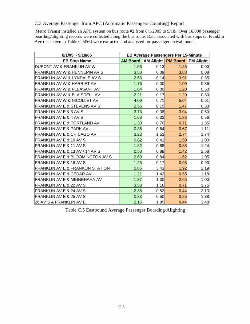
C-5

C.3 Average Passenger from APC (Automatic Passengers Counting) Report Metro Transit installed an APC system on bus route #2 from 8/1/2005 to 9/18/. Over 16,000 passenger boarding/alighting records were collected along the bus route. Data associated with bus stops on Franklin Ave (as shown in Table C.5&6) were extracted and analyzed for passenger arrival model.

8/1/05 ~ 9/18/05 EB Average Passengers Per 15-Minute EB Stop Name AM Board AM Alight PM Board PM Alight

DUPONT AV & FRANKLIN AV W 1.56 0.13 1.25 0.00 FRANKLIN AV W & HENNEPIN AV S 3.50 0.09 3.83 0.08 FRANKLIN AV W & LYNDALE AV S 2.66 0.14 3.91 0.35 FRANKLIN AV W & HARRIET AV 1.76 0.00 1.00 0.36 FRANKLIN AV W & PLEASANT AV 1.64 0.00 1.20 0.50 FRANKLIN AV W & BLAISDELL AV 2.21 0.17 1.20 0.30 FRANKLIN AV W & NICOLLET AV 4.09 0.71 5.04 0.61 FRANKLIN AV E & STEVENS AV S 2.56 0.15 1.47 0.33 FRANKLIN AV E & 3 AV S 3.73 0.38 3.04 0.50 FRANKLIN AV E & 4 AV S 1.63 0.32 1.83 0.56 FRANKLIN AV E & PORTLAND AV 1.30 0.70 0.71 1.35 FRANKLIN AV E & PARK AV 0.86 0.64 0.67 1.11 FRANKLIN AV E & CHICAGO AV 3.23 1.53 2.74 1.74 FRANKLIN AV E & 10 AV S 0.82 0.41 1.50 1.00 FRANKLIN AV E & 11 AV S 1.82 0.85 0.88 1.24 FRANKLIN AV E & 13 AV / 14 AV S 0.58 0.88 1.42 2.58 FRANKLIN AV E & BLOOMINGTON AV S 2.60 0.84 1.62 1.05 FRANKLIN AV E & 16 AV S 1.25 0.17 0.93 0.93 FRANKLIN AV E & FRANKLIN STATION 0.86 3.43 1.92 2.19 FRANKLIN AV E & CEDAR AV 1.21 1.42 0.55 1.18 FRANKLIN AV E & MINNEHAHA AV 1.37 1.30 2.65 1.00 FRANKLIN AV E & 22 AV S 3.53 1.16 0.71 1.75 FRANKLIN AV E & 24 AV S 2.35 0.52 0.44 2.13 FRANKLIN AV E & 25 AV S 0.83 0.50 0.25 1.38 26 AV S & FRANKLIN AV E 2.15 1.85 0.44 3.48

Table C.5 Eastbound Average Passenger Boarding/Alighting

C-6

8/1/05 ~ 9/18/05 WB Average Passengers Per 15-Minute WB Stop Name AM Board AM Alight PM Board PM Alight

FRANKLIN AV E & 26 AV S 2.27 0.04 1.88 0.79 FRANKLIN AV E & 24 AV S 1.40 0.25 0.48 1.59 FRANKLIN AV E & 23 AV S 1.25 0.13 1.48 1.00 FRANKLIN AV E & 22 AV S 1.91 0.00 0.96 1.85 FRANKLIN AV E & MINNEHAHA / CEDAR AV 1.29 0.42 2.38 1.13 FRANKLIN AV E & FRANKLIN STATION 1.05 2.79 3.65 2.08 FRANKLIN AV E & 16 AV S 1.15 0.92 0.39 1.22 FRANKLIN AV E & BLOOMINGTON AV S 1.08 0.92 1.17 1.54 FRANKLIN AV E & 13 AV S 1.40 0.27 2.50 1.93 FRANKLIN AV E & 11 AV S 1.05 0.79 0.70 1.52 FRANKLIN AV E & 10 AV S 1.00 1.00 0.47 1.68 FRANKLIN AV E & CHICAGO AV 0.91 1.31 3.00 4.06 FRANKLIN AV E & PARK AV 1.24 0.47 0.75 0.95 FRANKLIN AV E & PORTLAND AV 1.05 0.63 0.90 1.40 FRANKLIN AV E & CLINTON AV 0.88 0.50 0.54 2.32 FRANKLIN AV E & 3 AV S 0.67 1.13 0.54 2.27 FRANKLIN AV E & 1 AV S 0.38 0.75 0.12 3.50 FRANKLIN AV W & NICOLLET AV 0.56 2.70 0.56 5.73 FRANKLIN AV W & PILLSBURY AV 0.43 1.21 0.05 1.60 FRANKLIN AV W & HARRIET AV 0.00 1.25 0.00 1.61 FRANKLIN AV W & LYNDALE AV S 0.00 1.85 0.17 3.57 HENNEPIN AV S & FRANKLIN AV W 0.00 2.00 0.00 3.17

Table C.6 Westbound Average Passenger Boarding/Alighting

APPENDIX D Arterial Network Balancing Program

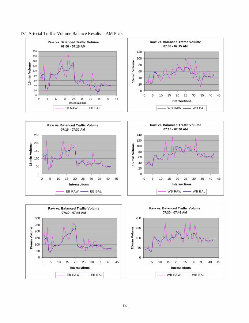
D-1

D.1 Arterial Traffic Volume Balance Results – AM Peak

Raw vs. Balanced Traffic Volume07:00 - 07:15 AM

0

20

40

60

80

100

120

140

160

180

0 5 10 15 20 25 30 35 40 45

Interse ctions

15-m

in V

olum

e

EB RAW EB BAL

Raw vs. Balanced Traffic Volume07:00 - 07:15 AM

0

20

40

60

80

100

120

0 5 10 15 20 25 30 35 40 45

Intersections

15-m

in V

olum

e

WB RAW WB BAL

Raw vs. Balanced Traffic Volume07:15 - 07:30 AM

0

50

100

150

200

250

0 5 10 15 20 25 30 35 40 45

Intersections

15-m

in V

olum

e

EB RAW EB BAL

Raw vs. Balanced Traffic Volume07:15 - 07:30 AM

0

20

40

60

80

100

120

140

0 5 10 15 20 25 30 35 40 45

Intersections

15-m

in V

olum

e

WB RAW WB BAL

Raw vs. Balanced Traffic Volume07:30 - 07:45 AM

0

50

100

150

200

250

300

0 5 10 15 20 25 30 35 40 45

Intersections

15-m

in V

olum

e

EB RAW EB BAL

Raw vs. Balanced Traffic Volume07:30 - 07:45 AM

0

50

100

150

200

0 5 10 15 20 25 30 35 40 45

Intersections

15-m

in V

olum

e

WB RAW WB BAL

D-2

Raw vs. Balanced Traffic Volume07:45 - 08:00 AM

0

50

100

150

200

250

300

0 5 10 15 20 25 30 35 40 45

Intersections

15-m

in V

olum

e

EB RAW EB BAL

Raw vs. Balanced Traffic Volume07:45 - 08:00 AM

0

50

100

150

200

250

300

350

0 5 10 15 20 25 30 35 40 45

Intersections

15-m

in V

olum

e

WB RAW WB BAL

Raw vs. Balanced Traffic Volume08:00 - 08:15 AM

0

50

100

150

200

250

0 5 10 15 20 25 30 35 40 45

Intersections

15-m

in V

olum

e

EB RAW EB BAL

Raw vs. Balanced Traffic Volume08:00 - 08:15 AM

0

50

100

150

200

250

300

0 5 10 15 20 25 30 35 40 45

Intersections

15-m

in V

olum

e

WB RAW WB BAL

Raw vs. Balanced Traffic Volume08:15 - 08:30 AM

0

50

100

150

200

250

0 5 10 15 20 25 30 35 40 45

Intersections

15-m

in V

olum

e

EB RAW EB BAL

Raw vs. Balanced Traffic Volume08:15 - 08:30 AM

0

50

100

150

200

250

0 5 10 15 20 25 30 35 40 45

Intersections

15-m

in V

olum

e

WB RAW WB BAL

D-3

Raw vs. Balanced Traffic Volume08:30 - 08:45 AM

0

50

100

150

200

250

300

0 5 10 15 20 25 30 35 40 45

Intersections

15-m

in V

olum

e

EB RAW EB BAL

Raw vs. Balanced Traffic Volume08:30 - 08:45 AM

0

50

100

150

200

250

300

0 5 10 15 20 25 30 35 40 45

Intersections

15-m

in V

olum

e

WB RAW WB BAL

Raw vs. Balanced Traffic Volume08:45 - 09:00 AM

0

50

100

150

200

250

0 5 10 15 20 25 30 35 40 45

Intersections

15-m

in V

olum

e

EB RAW EB BAL

Raw vs. Balanced Traffic Volume08:45 - 09:00 AM

0

50

100

150

200

250

0 5 10 15 20 25 30 35 40 45

Intersections

15-m

in V

olum

e

WB RAW WB BAL

D-4

D.2 Arterial Traffic Volume Balance Results – PM Peak

Raw vs. Balanced Traffic Volume04:00 - 04:15 PM

050

100150200250300350400

0 5 10 15 20 25 30 35 40 45

Intersections

15-m

in V

olum

e

EB RAW EB BAL

Raw vs. Balanced Traffic Volume04:00 - 04:15 PM

050

100150200250300350400

0 5 10 15 20 25 30 35 40 45

Intersections

15-m

in V

olum

e

WB RAW WB BAL

Raw vs. Balanced Traffic Volume04:15 - 04:30 PM

050

100150200250300350400

0 5 10 15 20 25 30 35 40 45

Intersections

15-m

in V

olum

e

EB RAW EB BAL

Raw vs. Balanced Traffic Volume04:15 - 04:30 PM

0

50

100

150

200

250

300

350

0 5 10 15 20 25 30 35 40 45

Intersections

15-m

in V

olum

e

WB RAW WB BAL

Raw vs. Balanced Traffic Volume04:30 - 04:45 PM

050

100150200250300350400450

0 5 10 15 20 25 30 35 40 45

Intersections

15-m

in V

olum

e

EB RAW EB BAL

Raw vs. Balanced Traffic Volume04:30 - 04:45 PM

050

100150200250300350400450500

0 5 10 15 20 25 30 35 40 45

Intersections

15-m

in V

olum

e

WB RAW WB BAL

D-5

Raw vs. Balanced Traffic Volume04:45 - 05:00 PM

050

100150200250300350400450500

0 5 10 15 20 25 30 35 40 45

Intersections

15-m

in V

olum

e

EB RAW EB BAL

Raw vs. Balanced Traffic Volume04:45 - 05:00 PM

050

100150200250300350400450500

0 5 10 15 20 25 30 35 40 45

Intersections

15-m

in V

olum

e

WB RAW WB BAL

Raw vs. Balanced Traffic Volume05:00 - 05:15 PM

050

100150200250300350400450

0 5 10 15 20 25 30 35 40 45

Intersections

15-m

in V

olum

e

EB RAW EB BAL

Raw vs. Balanced Traffic Volume05:00 - 05:15 PM

0

100

200

300

400

500

600

0 5 10 15 20 25 30 35 40 45

Intersections

15-m

in V

olum

e

WB RAW WB BAL

Raw vs. Balanced Traffic Volume05:15 - 05:30 PM

050

100150200

250300350400

0 5 10 15 20 25 30 35 40 45

Intersections

15-m

in V

olum

e

EB RAW EB BAL

Raw vs. Balanced Traffic Volume05:15 - 05:30 PM

050

100150200250300350400450500

0 5 10 15 20 25 30 35 40 45

Intersections

15-m

in V

olum

e

WB RAW WB BAL

D-6

Raw vs. Balanced Traffic Volume05:30 - 05:45 PM

0

50

100

150

200

250

300

350

0 5 10 15 20 25 30 35 40 45

Intersections

15-m

in V

olum

e

EB RAW EB BAL

Raw vs. Balanced Traffic Volume05:30 - 05:45 PM

050

100150200

250300

350400

0 5 10 15 20 25 30 35 40 45

Intersections

15-m

in V

olum

e

WB RAW WB BAL

Raw vs. Balanced Traffic Volume05:45 - 06:00 PM

0

50

100

150

200

250

300

0 5 10 15 20 25 30 35 40 45

Intersections

15-m

in V

olum

e

EB RAW EB BAL

Raw vs. Balanced Traffic Volume05:45 - 06:00 PM

050

100150200250300350400450

0 5 10 15 20 25 30 35 40 45

Intersections

15-m

in V

olum

e

WB RAW WB BAL

D-7

D.3 Java Program for Arterial Traffic Volume Balance /* * artbal.java * * Arterial traffic volume balance * Created on August 4, 2005, 9:42 AM */ /** * * @author Chen-Fu Liao */ import java.io.* ; public class artbal { /** Creates a new instance of artbal */ public artbal() { } /** * @param args the command line arguments */ public static void main(String[] args) { // TODO code application logic here String intsc_filename = args[0] ; String filepath = "" ; int num_states = 0 ; int num_intscs = 0 ; String[] data_files = null ; StateVol[][] traffic_vol = null ; StateVol[] tmpState = null ; System.out.println(intsc_filename) ; // read intersection filenames try { BufferedReader in = new BufferedReader(new FileReader(intsc_filename)) ; String str ; filepath = in.readLine() ; num_intscs = Integer.valueOf(in.readLine()).intValue() ; num_states = Integer.valueOf(in.readLine()).intValue() ; System.out.println(filepath + ", num_intscs = " + num_intscs + ", num_states = " + num_states) ; data_files = new String[num_intscs] ; /* while ((str = in.readLine()) != null) { System.out.println(str) ; } */ for (int i=0; i<num_intscs; i++) { data_files[i] = in.readLine() ; //System.out.println(data_files[i]) ; } in.close() ; } catch (IOException e) { System.out.println("Error: " + e.toString()) ; } // read all data files traffic_vol = new StateVol[num_states][num_intscs] ; tmpState = new StateVol[num_intscs] ; for (int i = 0; i<num_intscs; i++) { //num_intscs try { String str = filepath + data_files[i] ; // System.out.println(str) ; BufferedReader in = new BufferedReader(new FileReader(str)) ; // while ((str = in.readLine()) != null) { // System.out.println(str) ; // } // JAMAR headers for (int k=0; k<10; k++) { str = in.readLine() ; //System.out.println(str) ; } for (int k=0; k<num_states; k++) { str = in.readLine() ; int stidx = str.indexOf(",") ; //System.out.println(str.substring(0, stidx)) ; // initialize traffic_vol[k][i] traffic_vol[k][i] = new StateVol() ; traffic_vol[k][i].timestamp = str.substring(0, stidx) ; int[] sVolume = new int[16] ; str = str.substring(stidx+1) ; // System.out.println(str) ; int j=0, startidx = 0, endidx = 0 ;

for (j=0; j<15; j++) { endidx = str.indexOf(",", startidx) ; sVolume[j] = Integer.valueOf(str.substring(startidx, endidx)).intValue() ; startidx = endidx+1 ; } sVolume[j] = Integer.valueOf(str.substring(startidx)).intValue() ; //System.out.println(str) ; /* for (j=0; j<16; j++) { System.out.print(sVolume[j]+"-") ; } */ traffic_vol[k][i].setSB(sVolume[0], sVolume[1], sVolume[2], sVolume[3]) ; traffic_vol[k][i].setWB(sVolume[4], sVolume[5], sVolume[6], sVolume[7]) ; traffic_vol[k][i].setNB(sVolume[8], sVolume[9], sVolume[10], sVolume[11]) ; traffic_vol[k][i].setEB(sVolume[12], sVolume[13], sVolume[14], sVolume[15]) ; //printState(traffic_vol[k][i]) ; } // for k states in.close() ; } catch (IOException e) { System.out.println("Error: " +data_files[i] +", " + e.toString()) ; } } // for i intersection System.out.println("Data Files Loaded !") ; for (int k=0; k<num_states; k++) { // num_states // balance EB traffic // save a copy of current state for (int i=0; i<num_intscs; i++) { tmpState[i] = new StateVol() ; //printState(traffic_vol[k][i]) ; tmpState[i].setState(traffic_vol[k][i]) ; } // i num of intscs double error =0f ; int iter = 0 ; do { error = 0 ; for (int i=0; i<num_intscs-1; i++) { // num_intscs-1 float sum_inp, sum_out, diff, sum ; float SBL, EBT, NBR ; float oEBR, oEBT, oEBL ; SBL = traffic_vol[k][i].getSB().getLT() ; EBT = traffic_vol[k][i].getEB().getThru() ; NBR = traffic_vol[k][i].getNB().getRT() ; sum_inp = SBL + EBT + NBR ; oEBR = traffic_vol[k][i+1].getEB().getRT() ; oEBT = traffic_vol[k][i+1].getEB().getThru() ; oEBL = traffic_vol[k][i+1].getEB().getLT() ; sum_out = oEBR + oEBT + oEBL ; sum = sum_inp+sum_out ; diff = sum_out - sum_inp ; SBL += diff*SBL/sum ; EBT += diff*EBT/sum ; NBR += diff*NBR/sum ; oEBR -= diff*oEBR/sum ; oEBT -= diff*oEBT/sum ; oEBL -= diff*oEBL/sum ; traffic_vol[k][i].setSBL(SBL) ; traffic_vol[k][i].setEBT(EBT) ; traffic_vol[k][i].setNBR(NBR) ; traffic_vol[k][i+1].setEBL(oEBL) ; traffic_vol[k][i+1].setEBT(oEBT) ; traffic_vol[k][i+1].setEBR(oEBR) ; // printState(traffic_vol[k][i]) ; //printState(traffic_vol[k][i+1]) ; error += compareState(tmpState[i], traffic_vol[k][i]) ; } // i System.out.println("EB converge error:" + error) ; // save a copy for later comparison for (int i=0; i<num_intscs; i++) {

D-8

tmpState[i].setState(traffic_vol[k][i]) ; } // i num of intscs iter++ ; //System.out.println("----- iter = " + iter ) ; } while (error > 0.01 && iter < 100) ; // while System.out.println("EB balancing iter = " + iter ) ; // balance WB traffic iter = 0 ; do { error = 0 ; for (int i=num_intscs-1; i>0; i--) { // num_intscs-1 float sum_inp, sum_out, diff, sum ; float SBR, WBT, NBL ; float oWBR, oWBT, oWBL ; SBR = traffic_vol[k][i].getSB().getRT() ; WBT = traffic_vol[k][i].getWB().getThru() ; NBL = traffic_vol[k][i].getNB().getLT() ; sum_inp = SBR + WBT + NBL ; oWBR = traffic_vol[k][i-1].getWB().getRT() ; oWBT = traffic_vol[k][i-1].getWB().getThru() ; oWBL = traffic_vol[k][i-1].getWB().getLT() ; sum_out = oWBR + oWBT + oWBL ; sum = sum_inp+sum_out ; diff = sum_out - sum_inp ; SBR += diff*SBR/sum ; WBT += diff*WBT/sum ; NBL += diff*NBL/sum ; oWBR -= diff*oWBR/sum ; oWBT -= diff*oWBT/sum ; oWBL -= diff*oWBL/sum ; traffic_vol[k][i].setSBR(SBR) ; traffic_vol[k][i].setWBT(WBT) ; traffic_vol[k][i].setNBL(NBL) ; traffic_vol[k][i-1].setWBL(oWBL) ; traffic_vol[k][i-1].setWBT(oWBT) ; traffic_vol[k][i-1].setWBR(oWBR) ; // printState(traffic_vol[k][i]) ; //printState(traffic_vol[k][i+1]) ; error += compareState(tmpState[i], traffic_vol[k][i]) ; } // i System.out.println("WB converge error:" + error) ; // save a copy for later comparison for (int i=0; i<num_intscs; i++) { tmpState[i].setState(traffic_vol[k][i]) ; } // i num of intscs iter++ ; //System.out.println("----- iter = " + iter ) ; } while (error > 0.01 && iter < 100) ; // while System.out.println("WB balancing iter = " + iter ) ; } // num of states String out_filename = "" ; // save to output files in orginal time interval for (int id=0; id<num_intscs; id++) { try { out_filename = filepath + "balanced/" + data_files[id] + ".csv" ; BufferedWriter out = new BufferedWriter(new FileWriter(out_filename)) ; // System.out.println("out="+out_filename) ; out.write("Time, SBR, SBT, SBL, SB_tot, WBR, WBT, WBL, WB_tot, " + "NBR, NBT, NBL, NB_tot, EBR, EBT, EBL, EB_tot\n") ; for (int is=0; is<num_states; is++) { // num_states out.write(traffic_vol[is][id].toDataString()+"\n") ; } // for is state index out.close() ; } catch (IOException e) { System.out.println("Error write to file: " + out_filename + ": " + e.toString()) ; } } // for id // save to output files in veh per hour for (int id=0; id<num_intscs; id++) { try {

out_filename = filepath + "balanced/hourly/" + data_files[id] + "T.csv" ; BufferedWriter out = new BufferedWriter(new FileWriter(out_filename)) ; // System.out.println("out="+out_filename) ; out.write("Time, SBR, SBT, SBL, SB_tot, WBR, WBT, WBL, WB_tot, " + "NBR, NBT, NBL, NB_tot, EBR, EBT, EBL, EB_tot\n") ; for (int is=0; is<num_states; is++) { // num_states out.write(traffic_vol[is][id].toHrDataString()+"\n") ; } // for is state index out.close() ; } catch (IOException e) { System.out.println("Error write to file: (veh/h) " + out_filename + ": " + e.toString()) ; } } // for id // save to output files in percentage for (int id=0; id<num_intscs; id++) { try { out_filename = filepath + "balanced/percent/" + data_files[id] + "P.csv" ; BufferedWriter out = new BufferedWriter(new FileWriter(out_filename)) ; // System.out.println("out="+out_filename) ; out.write("Time, SBR%, SBT%, SBL%, SB_tot%, WBR%, WBT%, WBL%, WB_tot%, " + "NBR%, NBT%, NBL%, NB_tot%, EBR%, EBT%, EBL%, EB_tot%\n") ; for (int is=0; is<num_states; is++) { // num_states out.write(traffic_vol[is][id].toPercentDataString()+"\n") ; } // for is state index out.close() ; } catch (IOException e) { System.out.println("Error write to file: (%) " + out_filename + ": " + e.toString()) ; } } // for id System.out.println("Intersection Traffic Data Balanced!") ; } // main public static double compareState(StateVol sLast, StateVol sCur) { double diff = 0f ; double diff_sq_sum =0f ; double RMS ; diff = sLast.getSB().getLT() - sCur.getSB().getLT() ; diff_sq_sum += diff*diff ; // System.out.println("diff="+diff) ; diff = sLast.getSB().getThru() - sCur.getSB().getThru() ; diff_sq_sum += diff*diff ; // System.out.println("diff="+diff) ; diff = sLast.getSB().getRT() - sCur.getSB().getRT() ; diff_sq_sum += diff*diff ; // System.out.println("diff="+diff) ; // System.out.println("diff_sum="+diff_sq_sum) ; diff = sLast.getWB().getLT() - sCur.getWB().getLT() ; diff_sq_sum += diff*diff ; diff = sLast.getWB().getThru() - sCur.getWB().getThru() ; diff_sq_sum += diff*diff ; diff = sLast.getWB().getRT() - sCur.getWB().getRT() ; diff_sq_sum += diff*diff ; // System.out.println("diff_sum="+diff_sq_sum) ; diff = sLast.getNB().getLT() - sCur.getNB().getLT() ; diff_sq_sum += diff*diff ; diff = sLast.getNB().getThru() - sCur.getNB().getThru() ; diff_sq_sum += diff*diff ; diff = sLast.getNB().getRT() - sCur.getNB().getRT() ; diff_sq_sum += diff*diff ; // System.out.println("diff_sum="+diff_sq_sum) ; diff = sLast.getEB().getLT() - sCur.getEB().getLT() ; diff_sq_sum += diff*diff ; // System.out.println("diff="+diff) ; diff = sLast.getEB().getThru() - sCur.getEB().getThru() ; diff_sq_sum += diff*diff ; // System.out.println("diff="+diff) ; diff = sLast.getEB().getRT() - sCur.getEB().getRT() ; diff_sq_sum += diff*diff ; // System.out.println("diff="+diff) ;

D-9

// System.out.println("diff_sum="+diff_sq_sum) ; RMS = Math.sqrt(diff_sq_sum/12.0) ; // System.out.println("RMS = "+RMS) ; return RMS ; } public static void printState(StateVol traffic) { String delim = "," ; System.out.print(traffic.getSB().getRT()+delim) ; System.out.print(traffic.getSB().getThru()+delim) ; System.out.print(traffic.getSB().getLT()+delim) ; System.out.print(traffic.getSB().getOther()+delim) ; System.out.print(traffic.getWB().getRT()+delim) ; System.out.print(traffic.getWB().getThru()+delim) ; System.out.print(traffic.getWB().getLT()+delim) ; System.out.print(traffic.getWB().getOther()+delim) ; System.out.print(traffic.getNB().getRT()+delim) ; System.out.print(traffic.getNB().getThru()+delim) ;

System.out.print(traffic.getNB().getLT()+delim) ; System.out.print(traffic.getNB().getOther()+delim) ; System.out.print(traffic.getEB().getRT()+delim) ; System.out.print(traffic.getEB().getThru()+delim) ; System.out.print(traffic.getEB().getLT()+delim) ; System.out.print(traffic.getEB().getOther()+delim+"\n") ; } public static int[] parseVol(String str) { int[] data = new int[16] ; int startidx = 0, endidx = 0 ; for (int i=0; i<16; i++) { endidx = str.indexOf(",") ; data[i] = Integer.valueOf(str.substring(startidx, endidx-1)).intValue() ; startidx = endidx+1 ; } return data ; } } // class

D.4 Sample Input File – intersections.txt /home/cliao/franklin/ 42 16 Dupont_I298.txt Colfax_070805.txt Hennepin_I297.txt Bryant_070605.txt Aldrich_070705.txt Lyndale_I381.txt Garfield_071205.txt Harriet_071105.txt Grand_070505.txt Pleasant_070105.txt Pillsbury_063005.txt Blaisdell_I49.txt Nicollet_I98.txt 1st_I833.txt Stevens_062905.txt 2nd_062805.txt 3rd_I236.txt Clinton_I254.txt 4th_I161.txt 5th_I347.txt

Portland_I187.txt Oakland_062705.txt Park_I256.txt Columbus_062405.txt Chicago_I489.txt Elliot_062305.txt 10th_062205.txt 11th_I491.txt 13thm_I492.txt 14th_062105.txt 15thm_I869.txt Bloomington_I845.txt 16th_062005.txt 17th_061705.txt Cedar_I203.txt Minnehaha_I206.txt 21st_061605.txt 22nd_I938.txt 23rd_061505.txt 24th_061405.txt 25th_061305.txt 26th_I44.txt

D.5 Traffic Volume Data Format – JAMAR Style Data File "Franklin" "00000000" "07/01/2005" "07:00" "Franklin Lyndale" "REF.PT.: 45.255" "JAMAR#631 re" "TURN MOVEMENT COUNT" "Movement 1= AUTO & TRUCK" "Key #", 1, 2, 3, 4, 5, 6, 7, 8, 9, 10, 11, 12, 13, 14, 15, 16 7:00,2,111,68,0,38,17,4,0,11,211,3,0,4,34,21,0 7:15,4,136,84,0,39,18,5,0,11,312,6,0,7,53,55,0 7:30,3,142,84,0,88,20,2,0,6,328,2,0,1,57,104,0

7:45,1,169,83,0,86,34,8,0,7,344,5,0,7,92,91,0 8:00,5,130,65,0,53,45,7,0,12,273,5,0,12,63,58,0 8:15,1,132,85,0,61,27,7,0,16,272,12,0,7,71,48,0 8:30,4,140,73,0,61,27,12,0,16,266,5,0,2,62,45,0 8:45,4,142,71,0,59,30,6,0,13,299,12,0,5,46,34,0 16:00,8,203,68,0,77,61,13,0,13,241,7,0,13,28,17,0 16:15,8,206,58,0,73,66,18,0,16,241,12,0,10,39,14,0 16:30,7,160,53,0,58,71,13,2,3,249,7,0,10,29,17,0 16:45,3,224,85,0,55,87,20,0,23,241,15,0,11,30,18,6 17:00,5,215,70,0,81,81,21,0,16,228,8,0,18,34,14,0 17:15,13,279,76,0,64,158,27,0,13,243,14,0,17,38,24,0 17:30,12,226,70,0,60,68,25,6,17,243,15,0,11,35,24,0 17:45,10,225,75,0,63,63,17,0,17,272,16,0,14,51,25,0

APPENDIX E

Traffic Volume Calibration Results

E-1

E.1 Detector Station ID assignment

The detector stations in the simulation were assigned as follows. Detector Intersection Detector Intersection Detector Intersection

Station ID Name Station ID Name Station ID Name 1 Dupont 15 Stevens 29 13th 2 Colfax 16 2nd 30 14th 3 Hennepin 17 3rd 31 15th 4 Bryant 18 Clinton 32 Bloomington 5 Aldrich 19 4th 33 16th 6 Lyndale 20 5th 34 17th 7 Garfield 21 Portland 35 Cedar 8 Harriet 22 Oakland 36 Minnehaha 9 Grand 23 Park 37 21st 10 Pleasant 24 Columbus 38 22nd 11 Pillsbury 25 Chicago 39 23rd 12 Blaisdell 26 Elliot 40 24th 13 Nicollet 27 10th 41 25th 14 1st 28 11th 42 26th

Table E.1 Detector Station ID Assignment E.2 Capacity Calibration Results – AM Peak

The capacity calibration results for each 15-minute interval were plotted as follows where the reaction time (simulation step) was 0.75 sec and reaction time at stop in the simulation model was 0.80 sec.

E-2

07:00 ~ 07:15 AM EB

0

20

40

60

80

100

120

140

1601 3 5 7 9 11 13 15 17 19 21 23 25 27 29 31 33 35 37 39 41

Detector Station

15-m

in V

olum

e

EB SIM EB BAL

07:00 ~ 07:15AM WB

0102030405060708090

100

1 3 5 7 9 11 13 15 17 19 21 23 25 27 29 31 33 35 37 39 41

Detector Station

15-m

in V

olum

e

WB SIM WB BAL

07:15 ~ 07:30AM EB

020406080

100120140160180200

1 3 5 7 9 11 13 15 17 19 21 23 25 27 29 31 33 35 37 39 41

Detector Station

15-m

in V

olum

e

EB SIM EB BAL

07:15 ~ 07:30AM WB

0

20

40

60

80

100

120

1 3 5 7 9 11 13 15 17 19 21 23 25 27 29 31 33 35 37 39 41

Detector Station

15-m

in V

olum

e

WB SIM WB BAL

07:30 ~ 07:45AM EB

0

50

100

150

200

250

1 3 5 7 9 11 13 15 17 19 21 23 25 27 29 31 33 35 37 39 41

Detector Station

15-m

in V

olum

e

EB SIM EB BAL

07:30 ~ 07:45AM WB

0

20

40

60

80

100

120

140

160

1 3 5 7 9 11 13 15 17 19 21 23 25 27 29 31 33 35 37 39 41

Detector Station

15-m

in V

olum

e

WB SIM WB BAL

07:45 ~ 08:00AM EB

0

50

100

150

200

250

300

1 3 5 7 9 11 13 15 17 19 21 23 25 27 29 31 33 35 37 39 41

Detector Station

15-m

in V

olum

e

EB SIM EB BAL

07:45 ~ 08:00AM WB

0

20

40

60

80

100

120

140

160

1 3 5 7 9 11 13 15 17 19 21 23 25 27 29 31 33 35 37 39 41

Detector Station

15-m

in V

olum

e

WB SIM WB BAL

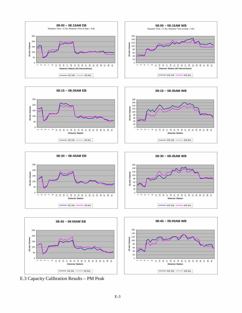
E-3

08:00 ~ 08:15AM EBReaction Time = 0.75s, Reaction Time at Stop = 0.8s

0

50

100

150

200

2501 3 5 7 9 11 13 15 17 19 21 23 25 27 29 31 33 35 37 39 41

Detector Station (42 intersections)

15-m

in V

olum

e

EB SIM EB BAL

08:00 ~ 08:15AM WBReaction Time = 0.75s, Reaction Time at Stop = 0.8s

0

20

40

60

80

100

120

140

160

1 3 5 7 9 11 13 15 17 19 21 23 25 27 29 31 33 35 37 39 41

Detector Station (42 intersections)

15-m

in V

olum

e

WB SIM WB BAL

08:15 ~ 08:30AM EB

0

50

100

150

200

250

1 3 5 7 9 11 13 15 17 19 21 23 25 27 29 31 33 35 37 39 41

Detector Station

15-m

in V

olum

e

EB SIM EB BAL

08:15 ~ 08:30AM WB

020406080

100120140160180

1 3 5 7 9 11 13 15 17 19 21 23 25 27 29 31 33 35 37 39 41

Detector Station

15-m

in V

olum

e

WB SIM WB BAL

08:30 ~ 08:45AM EB

0

50

100

150

200

250

1 3 5 7 9 11 13 15 17 19 21 23 25 27 29 31 33 35 37 39 41

Detector Station

15-m

in V

olum

e

EB SIM EB BAL

08:30 ~ 08:45AM WB

0

20

40

60

80

100

120

140

160

1 3 5 7 9 11 13 15 17 19 21 23 25 27 29 31 33 35 37 39 41

Detector Station

15-m

in V

olum

e

WB SIM WB BAL

08:45 ~ 09:00AM EB

0

50

100

150

200

250

1 3 5 7 9 11 13 15 17 19 21 23 25 27 29 31 33 35 37 39 41

Detector Statioin

15-m

in V

olum

e

EB SIM EB BAL

08:45 ~ 09:00AM WB

0

20

40

60

80

100

120

140

160

1 3 5 7 9 11 13 15 17 19 21 23 25 27 29 31 33 35 37 39 41

Detector Station

15-m

in V

olum

e

WB SIM WB BAL

E.3 Capacity Calibration Results – PM Peak

E-4

04:00 ~ 04:15PM EB

0

50

100

150

200

250

1 3 5 7 9 11 13 15 17 19 21 23 25 27 29 31 33 35 37 39 41

Detector Station

15-m

in V

olum

e

EB SIM EB BAL

04:00 ~ 04:15PM WB

0

50

100

150

200

250

1 3 5 7 9 11 13 15 17 19 21 23 25 27 29 31 33 35 37 39 41

Detector Station

15-m

in V

olum

e

WB SIM WB BAL

04:15 ~ 04:30PM EB

0

50

100

150

200

250

1 3 5 7 9 11 13 15 17 19 21 23 25 27 29 31 33 35 37 39 41

Detector Station

15-m

in V

olum

e

EB SIM EB BAL

04:15 ~ 04:30PM WB

0

50

100

150

200

250

300

1 3 5 7 9 11 13 15 17 19 21 23 25 27 29 31 33 35 37 39 41

Detector Station

15-m

in V

olum

e

WB SIM WB BAL

04:30 ~ 04:45PM EB

0

50

100

150

200

250

300

1 3 5 7 9 11 13 15 17 19 21 23 25 27 29 31 33 35 37 39 41

Detector Station

15-m

in V

olum

e

EB SIM EB BAL

04:30 ~ 04:45PM WB

0

50

100

150

200

250

300

1 3 5 7 9 11 13 15 17 19 21 23 25 27 29 31 33 35 37 39 41

Detector Station

15-m

in V

olum

e

WB SIM WB BAL

04:45 ~ 05:00PM EB

0

50

100

150

200

250

300

1 3 5 7 9 11 13 15 17 19 21 23 25 27 29 31 33 35 37 39 41

Detector Station

15-m

in V

olum

e

EB SIM EB BAL

04:45 ~ 05:00PM WB

0

50

100

150

200

250

300

1 3 5 7 9 11 13 15 17 19 21 23 25 27 29 31 33 35 37 39 41

Detector Station

15-m

in V

olum

e

WB SIM WB BAL

E-5

05:00 ~ 05:15PM EB

0

50

100

150

200

250

300

1 3 5 7 9 11 13 15 17 19 21 23 25 27 29 31 33 35 37 39 41

Detector Station

15-m

in V

olum

e

EB SIM EB BAL

05:00 ~ 05:15PM WB

0

50

100

150

200

250

300

350

1 3 5 7 9 11 13 15 17 19 21 23 25 27 29 31 33 35 37 39 41

Detector Station

15-m

in V

olum

e

WB SIM WB BAL

05:15 ~ 05:30PM EB

0

50

100

150

200

250

300

1 3 5 7 9 11 13 15 17 19 21 23 25 27 29 31 33 35 37 39 41

Detector Station

15-m

in V

olum

e

EB SIM EB BAL

05:15 ~ 05:30PM WB

0

50

100

150

200

250

300

350

1 3 5 7 9 11 13 15 17 19 21 23 25 27 29 31 33 35 37 39 41

Detector Station

15-m

in V

olum

e

WB SIM WB BAL

05:30 ~ 05:45PM EB

0

50

100

150

200

250

300

1 3 5 7 9 11 13 15 17 19 21 23 25 27 29 31 33 35 37 39 41

Detector Station

15-m

in V

olum

e

EB SIM EB BAL

05:30 ~ 05:45PM WB

0

50

100

150

200

250

300

1 3 5 7 9 11 13 15 17 19 21 23 25 27 29 31 33 35 37 39 41

Detector Station

15-m

in V

olum

e

WB SIM WB BAL

05:45 ~ 06:00PM EB

0

50

100

150

200

250

300

1 3 5 7 9 11 13 15 17 19 21 23 25 27 29 31 33 35 37 39 41

Detector Station

15-m

in V

olum

e

EB SIM EB BAL

05:45 ~ 06:00PM WB

0

50

100

150

200

250

300

1 3 5 7 9 11 13 15 17 19 21 23 25 27 29 31 33 35 37 39 41

Detector Station

15-m

in V

olum

e

WB SIM WB BAL

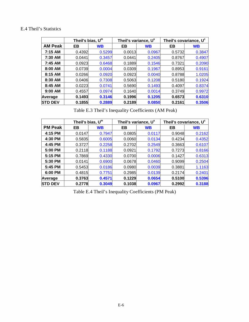
E-6

E.4 Theil’s Statistics

Theil's bias, Um Theil's variance, Us Theil's covariance, Uc

AM Peak EB WB EB WB EB WB 7:15 AM 0.4392 0.5299 0.0013 0.0967 0.5732 0.3847 7:30 AM 0.0441 0.3457 0.0441 0.2405 0.8767 0.4907 7:45 AM 0.0923 0.6468 0.1889 0.1546 0.7321 0.2090 8:00 AM 0.0739 0.0004 0.0309 0.1967 0.8953 0.9161 8:15 AM 0.0266 0.0920 0.0923 0.0040 0.8788 1.0205 8:30 AM 0.0406 0.7308 0.5063 0.1208 0.5180 0.1924 8:45 AM 0.0223 0.0741 0.5690 0.1493 0.4097 0.8374 9:00 AM 0.4557 0.0974 0.1640 0.0014 0.3749 0.9972

Average 0.1493 0.3146 0.1996 0.1205 0.6573 0.6310 STD DEV 0.1855 0.2889 0.2189 0.0850 0.2161 0.3506

Table E.3 Theil’s Inequality Coefficients (AM Peak)

Theil's bias, Um Theil's variance, Us Theil's covariance, Uc PM Peak EB WB EB WB EB WB 4:15 PM 0.0147 0.7947 0.0805 0.0117 0.9048 0.2162 4:30 PM 0.5835 0.6005 0.0060 0.0134 0.4234 0.4352 4:45 PM 0.3727 0.2258 0.2702 0.2549 0.3663 0.6107 5:00 PM 0.2118 0.1188 0.0921 0.1792 0.7273 0.8166 5:15 PM 0.7869 0.4330 0.0700 0.0006 0.1427 0.6313 5:30 PM 0.0141 0.6900 0.0678 0.0460 0.9099 0.2504 5:45 PM 0.5453 0.0186 0.0980 0.0039 0.3881 1.1163 6:00 PM 0.4815 0.7751 0.2985 0.0139 0.2174 0.2401

Average 0.3763 0.4571 0.1229 0.0654 0.5100 0.5396 STD DEV 0.2778 0.3049 0.1038 0.0967 0.2992 0.3188

Table E.4 Theil’s Inequality Coefficients (PM Peak)