Bundle Adjustment and System Calibration with Points at ... · Bundle Adjustment and System...
13
PFG 2013 / 4, 0309 – 0321 Stuttgart, August 2013 Article Bundle Adjustment and System Calibration with Points at Infinity for Omnidirectional Camera Systems J OHANNES SCHNEIDER &WOLFGANG F¨ ORSTNER, Keywords: bundle adjustment, omnidirectional camera systems, multi-view cameras, calibration Summary: We present a calibration method for multi-view cameras that provides a rigorous maxi- mum likelihood estimation of the mutual orientation of the cameras within a rigid multi-camera system. No calibration targets are needed, just a movement of the multi-camera system taking synchronized images of a highly textured and static scene. Multi-camera systems with non-overlapping views have to be ro- tated within the scene so that corresponding points are visible in different cameras at different times of exposure. By using an extended version of the pro- jective collinearity equation all estimates can be opti- mized in one bundle adjustment where we constrain the relative poses of the cameras to be fixed. For sta- bilizing camera orientations – especially rotations – one should generally use points at the horizon within the bundle adjustment, which classical bundle adjust- ment programs are not capable of. We use a minimal representation of homogeneous coordinates for im- age and scene points which allows us to use images of omnidirectional cameras with single viewpoint like fisheye cameras and scene points at a large distance from the camera or even at infinity. We show results of our calibration method on (1) the omnidirectional multi-camera system Ladybug 3 from Point Grey, (2) a camera-rig with five cameras used for the acquisition of complex 3D structures and (3) a camera-rig mounted on a UAV consisting of four fisheye cameras which provide a large field of view and which is used for visual odometry and obsta- cle detection in the project MoD (DFG-Project FOR 1505 “Mapping on Demand”). Zusammenfassung: B¨ undelausgleichung und Sys- temkalibrierung mit Punkten im Unendlichen f¨ ur omnidirektionale Kamerasysteme. In diesem Artikel stellen wir eine Kalibrierungsmethode f¨ ur Multika- merasysteme vor, welche eine strenge Maximum- Likelihood-Sch¨ atzung der gegenseitigen Orientierun- gen der Kameras innerhalb eines starren Multika- merasystems erm¨ oglicht. Zielmarken werden nicht ben¨ otigt. Das synchronisiert Bilder aufnehmende Ka- merasystem muss lediglich in einer stark texturier- ten statischen Szene bewegt werden. Multikamera- systeme, deren Bilder sich nicht ¨ uberlappen, wer- den innerhalb der Szene rotiert, so dass korrespon- dierende Punkte in jeder Kamera zu unterschiedli- chen Aufnahmezeitpunkten sichtbar sind. Unter Ver- wendung einer erweiterten projektiven Kollinearit¨ ats- gleichung k¨ onnen alle zu sch¨ atzenden Gr¨ oßen in ei- ner B¨ undelausgleichung optimiert werden. Zur Sta- bilisierung der Kameraorientierungen – besonders der Rotationen – sollten Punkte am Horizont in der B¨ undelausgleichung verwendet werden, wozu klas- sische B¨ undelausgleichungsprogramme nicht in der Lage sind. Wir benutzen eine minimale Repr¨ asentati- on f¨ ur homogene Koordinaten f¨ ur Bild- und Objekt- punkte, welche es uns erm¨ oglicht, mit Bildern omni- direktionaler Kameras wie Fisheye-Kameras und mit Objektpunkten, welche weit entfernt oder im Unend- lichen liegen, umzugehen. Wir zeigen Ergebnisse unserer Kalibrierungsme- thode f¨ ur (1) das omnidirektionale Multikamerasys- tem Ladybug3 von Point Grey, (2) ein Kamerasys- tem mit f¨ unf Kameras zur Aufnahme komplexer 3D- Strukturen und (3) ein auf eine Drohne montiertes Kamerasystem mit vier Fisheye-Kameras, welches ein großes Sichtfeld besitzt und zur visuellen Odo- metrie und zur Hinderniserkennung im Projekt MoD (DFG-Projekt FOR 1505 ” Mapping on Demand“) verwendet wird. c 2013 E. Schweizerbart’sche Verlagsbuchhandlung, Stuttgart, Germany DOI: 10.1127/1432-8364/2013/0179 www.schweizerbart.de 1432-8364/13/0179 $ 3.25 B Bonn
Transcript of Bundle Adjustment and System Calibration with Points at ... · Bundle Adjustment and System...
PFG 2013 / 4, 0309 –0321Stuttgart, August 2013
Article
Bundle Adjustment and System Calibration withPoints at Infinity for Omnidirectional Camera Systems
JOHANNES SCHNEIDER & WOLFGANG FORSTNER,
Keywords: bundle adjustment, omnidirectional camera systems, multi-view cameras, calibration
Summary: We present a calibration method for
multi-view cameras that provides a rigorous maxi-
mum likelihood estimation of the mutual orientation
of the cameras within a rigid multi-camera system.
No calibration targets are needed, just a movement of
the multi-camera system taking synchronized images
of a highly textured and static scene. Multi-camera
systems with non-overlapping views have to be ro-
tated within the scene so that corresponding points
are visible in different cameras at different times of
exposure. By using an extended version of the pro-
jective collinearity equation all estimates can be opti-
mized in one bundle adjustment where we constrain
the relative poses of the cameras to be fixed. For sta-
bilizing camera orientations – especially rotations –
one should generally use points at the horizon within
the bundle adjustment, which classical bundle adjust-
ment programs are not capable of. We use a minimal
representation of homogeneous coordinates for im-
age and scene points which allows us to use images of
omnidirectional cameras with single viewpoint like
fisheye cameras and scene points at a large distance
from the camera or even at infinity.
We show results of our calibration method on (1)
the omnidirectional multi-camera system Ladybug 3
from Point Grey, (2) a camera-rig with five cameras
used for the acquisition of complex 3D structures and
(3) a camera-rig mounted on a UAV consisting of four
fisheye cameras which provide a large field of view
and which is used for visual odometry and obsta-
cle detection in the project MoD (DFG-Project FOR
1505 “Mapping on Demand”).
Zusammenfassung: Bundelausgleichung und Sys-temkalibrierung mit Punkten im Unendlichen furomnidirektionale Kamerasysteme. In diesem Artikel
stellen wir eine Kalibrierungsmethode fur Multika-
merasysteme vor, welche eine strenge Maximum-
Likelihood-Schatzung der gegenseitigen Orientierun-
gen der Kameras innerhalb eines starren Multika-
merasystems ermoglicht. Zielmarken werden nicht
benotigt. Das synchronisiert Bilder aufnehmende Ka-
merasystem muss lediglich in einer stark texturier-
ten statischen Szene bewegt werden. Multikamera-
systeme, deren Bilder sich nicht uberlappen, wer-
den innerhalb der Szene rotiert, so dass korrespon-
dierende Punkte in jeder Kamera zu unterschiedli-
chen Aufnahmezeitpunkten sichtbar sind. Unter Ver-
wendung einer erweiterten projektiven Kollinearitats-
gleichung konnen alle zu schatzenden Großen in ei-
ner Bundelausgleichung optimiert werden. Zur Sta-
bilisierung der Kameraorientierungen – besonders
der Rotationen – sollten Punkte am Horizont in der
Bundelausgleichung verwendet werden, wozu klas-
sische Bundelausgleichungsprogramme nicht in der
Lage sind. Wir benutzen eine minimale Reprasentati-
on fur homogene Koordinaten fur Bild- und Objekt-
punkte, welche es uns ermoglicht, mit Bildern omni-
direktionaler Kameras wie Fisheye-Kameras und mit
Objektpunkten, welche weit entfernt oder im Unend-
lichen liegen, umzugehen.
Wir zeigen Ergebnisse unserer Kalibrierungsme-
thode fur (1) das omnidirektionale Multikamerasys-
tem Ladybug 3 von Point Grey, (2) ein Kamerasys-
tem mit funf Kameras zur Aufnahme komplexer 3D-
Strukturen und (3) ein auf eine Drohne montiertes
Kamerasystem mit vier Fisheye-Kameras, welches
ein großes Sichtfeld besitzt und zur visuellen Odo-
metrie und zur Hinderniserkennung im Projekt MoD
(DFG-Projekt FOR 1505”Mapping on Demand“)
verwendet wird.
c© 2013 E. Schweizerbart’sche Verlagsbuchhandlung, Stuttgart, Germany
DOI: 10.1127/1432-8364/2013/0179www.schweizerbart.de
1432-8364/13/0179 $ 3.25
BBonn
310 Photogrammetrie • Fernerkundung • Geoinformation 4/2013
1 Introduction
1.1 Motivation
The paper presents a rigorous bundle adjust-
ment for the estimation of the mutual camera
orientations in a rigid multi-camera system. It is
based on an extended version of the projective
collinearity equation which constrains the rela-
tive poses of the cameras to be fixed, whereby
all estimates can be optimized in one bundle
adjustment. Further it enables the use of im-
age and scene points at infinity like the bundle
adjustment “BACS” (Bundle Adjustment for
Camera Systems) presented in SCHNEIDER et
al. (2012).
Bundle adjustment is the work horse for ori-
enting cameras and determining 3D points. It
has a number of favourable properties: It is sta-
tistically optimal in case all statistical tools are
exploited, highly efficient in case sparse matrix
operations are used, useful for test field free self
calibration, and can be parallelized to a high de-
gree. In this paper we want to extend bundle
adjustment with the estimation of the parame-
ters of the mutual camera orientation in a multi-
camera system.
Multi-camera systems are used to increase
the resolution, to combine cameras with dif-
ferent spectral sensitivities (Z/I DMC, Vexcel
Ultracam) or – like omnidirectional cameras –
to augment the effective aperture angle (Blom
Pictometry, Rollei Panoscan Mark III). Fol-
lowing SCARAMUZZA (2008), omnidirectional
cameras have a viewing range of more than
a half-sphere, such as multi-cameras systems,
catadioptric cameras including mirrors, or also
special fisheye lenses, such as the Lensagon
BF2M15520. Additionally, multi-camera sys-
tems gain importance for the acquisition of
complex 3D structures.
Far or even ideal points, i.e. points at infinity,
e.g. points at the horizon or luminous stars are
effective in stabilizing the orientation of cam-
eras, especially their rotations.
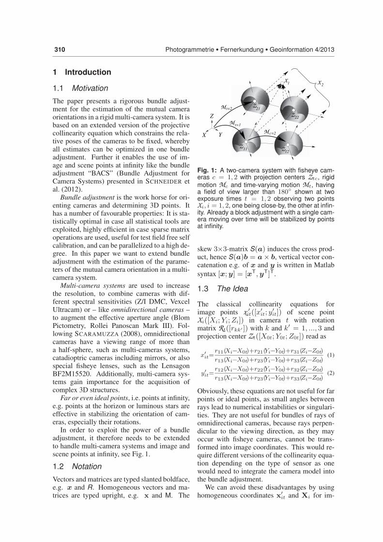
In order to exploit the power of a bundle
adjustment, it therefore needs to be extended
to handle multi-camera systems and image and
scene points at infinity, see Fig. 1.
1.2 Notation
Vectors and matrices are typed slanted boldface,
e.g. x and R. Homogeneous vectors and ma-
trices are typed upright, e.g. x and M. The
Fig. 1: A two-camera system with fisheye cam-eras c = 1, 2 with projection centers Ztc, rigidmotion Mc and time-varying motion Mt, havinga field of view larger than 180◦ shown at twoexposure times t = 1, 2 observing two pointsXi, i = 1, 2, one being close-by, the other at infin-ity. Already a block adjustment with a single cam-era moving over time will be stabilized by pointsat infinity.
skew 3×3-matrix S(a) induces the cross prod-
uct, hence S(a)b = a× b, vertical vector con-
catenation e.g. of x and y is written in Matlab
syntax [x;y] = [xT,yT]T.
1.3 The Idea
The classical collinearity equations for
image points x ′it([x
′it; y
′it]) of scene point
Xi([Xi;Yi;Zi]) in camera t with rotation
matrix Rt([rkk′ ]) with k and k′ = 1, ..., 3 and
projection center Zt([X0t;Y0t;Z0t]) read as
x′it=r11(Xi−X0t)+r21(Yi−Y0t)+r31(Zi−Z0t)
r13(Xi−X0t)+r23(Yi−Y0t)+r33(Zi−Z0t)(1)
y′it=r12(Xi−X0t)+r22(Yi−Y0t)+r32(Zi−Z0t)
r13(Xi−X0t)+r23(Yi−Y0t)+r33(Zi−Z0t)(2)
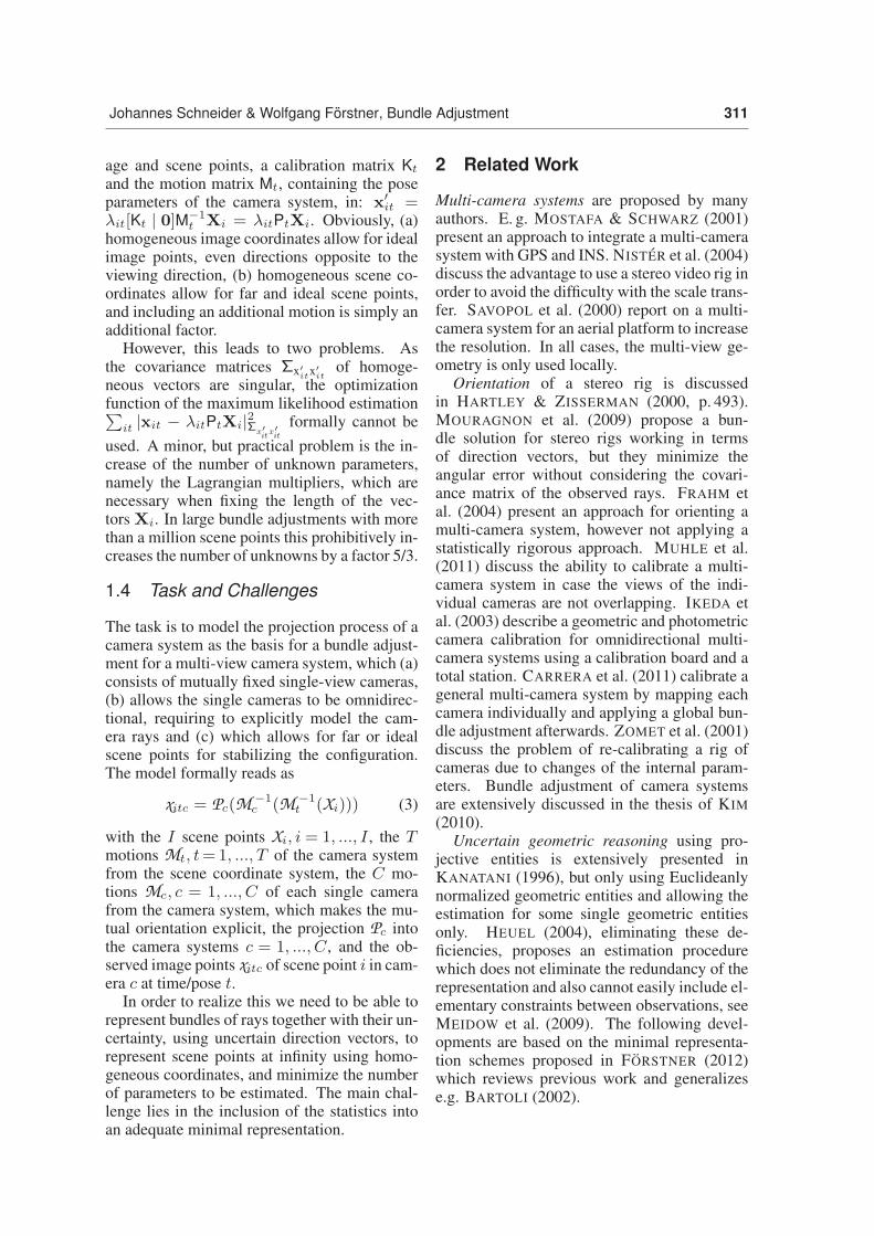
Obviously, these equations are not useful for far
points or ideal points, as small angles between
rays lead to numerical instabilities or singulari-
ties. They are not useful for bundles of rays of
omnidirectional cameras, because rays perpen-
dicular to the viewing direction, as they may
occur with fisheye cameras, cannot be trans-
formed into image coordinates. This would re-
quire different versions of the collinearity equa-
tion depending on the type of sensor as one
would need to integrate the camera model into
the bundle adjustment.
We can avoid these disadvantages by using
homogeneous coordinates x′it and Xi for im-
Johannes Schneider & Wolfgang Forstner, Bundle Adjustment 311
age and scene points, a calibration matrix Kt
and the motion matrix Mt, containing the pose
parameters of the camera system, in: x′it =
λit[Kt | 0]M−1t Xi = λitPtXi. Obviously, (a)
homogeneous image coordinates allow for ideal
image points, even directions opposite to the
viewing direction, (b) homogeneous scene co-
ordinates allow for far and ideal scene points,
and including an additional motion is simply an
additional factor.
However, this leads to two problems. As
the covariance matrices Σx′itx′
itof homoge-
neous vectors are singular, the optimization
function of the maximum likelihood estimation∑it |xit − λitPtXi|2Σx′
itx′it
formally cannot be
used. A minor, but practical problem is the in-
crease of the number of unknown parameters,
namely the Lagrangian multipliers, which are
necessary when fixing the length of the vec-
tors Xi. In large bundle adjustments with more
than a million scene points this prohibitively in-
creases the number of unknowns by a factor 5/3.
1.4 Task and Challenges
The task is to model the projection process of a
camera system as the basis for a bundle adjust-
ment for a multi-view camera system, which (a)
consists of mutually fixed single-view cameras,
(b) allows the single cameras to be omnidirec-
tional, requiring to explicitly model the cam-
era rays and (c) which allows for far or ideal
scene points for stabilizing the configuration.
The model formally reads as
xitc = Pc(M −1c (M −1
t (Xi))) (3)
with the I scene points Xi, i = 1, ..., I , the Tmotions Mt, t=1, ..., T of the camera system
from the scene coordinate system, the C mo-
tions Mc, c = 1, ..., C of each single camera
from the camera system, which makes the mu-
tual orientation explicit, the projection Pc into
the camera systems c = 1, ..., C, and the ob-
served image points xitc of scene point i in cam-
era c at time/pose t.In order to realize this we need to be able to
represent bundles of rays together with their un-
certainty, using uncertain direction vectors, to
represent scene points at infinity using homo-
geneous coordinates, and minimize the number
of parameters to be estimated. The main chal-
lenge lies in the inclusion of the statistics into
an adequate minimal representation.
2 Related Work
Multi-camera systems are proposed by many
authors. E. g. MOSTAFA & SCHWARZ (2001)
present an approach to integrate a multi-camera
system with GPS and INS. NISTER et al. (2004)
discuss the advantage to use a stereo video rig in
order to avoid the difficulty with the scale trans-
fer. SAVOPOL et al. (2000) report on a multi-
camera system for an aerial platform to increase
the resolution. In all cases, the multi-view ge-
ometry is only used locally.
Orientation of a stereo rig is discussed
in HARTLEY & ZISSERMAN (2000, p. 493).
MOURAGNON et al. (2009) propose a bun-
dle solution for stereo rigs working in terms
of direction vectors, but they minimize the
angular error without considering the covari-
ance matrix of the observed rays. FRAHM et
al. (2004) present an approach for orienting a
multi-camera system, however not applying a
statistically rigorous approach. MUHLE et al.
(2011) discuss the ability to calibrate a multi-
camera system in case the views of the indi-
vidual cameras are not overlapping. IKEDA et
al. (2003) describe a geometric and photometric
camera calibration for omnidirectional multi-
camera systems using a calibration board and a
total station. CARRERA et al. (2011) calibrate a
general multi-camera system by mapping each
camera individually and applying a global bun-
dle adjustment afterwards. ZOMET et al. (2001)
discuss the problem of re-calibrating a rig of
cameras due to changes of the internal param-
eters. Bundle adjustment of camera systems
are extensively discussed in the thesis of KIM
(2010).
Uncertain geometric reasoning using pro-
jective entities is extensively presented in
KANATANI (1996), but only using Euclideanly
normalized geometric entities and allowing the
estimation for some single geometric entities
only. HEUEL (2004), eliminating these de-
ficiencies, proposes an estimation procedure
which does not eliminate the redundancy of the
representation and also cannot easily include el-
ementary constraints between observations, see
MEIDOW et al. (2009). The following devel-
opments are based on the minimal representa-
tion schemes proposed in FORSTNER (2012)
which reviews previous work and generalizes
e.g. BARTOLI (2002).
312 Photogrammetrie • Fernerkundung • Geoinformation 4/2013
3 Concept
3.1 Model for a moving single-viewCamera
3.1.1 Image coordinates as observations
Using homogeneous coordinates
x′it = λitPtXi = λitKtR
Tt [I3 | −Zt]Xi (4)
with a projection matrix
Pt = [Kt | 03×1]M−1t , Mt =
[Rt Zt
0T 1
]makes the motion of the camera explicit. It
contains for each pose t: the projection center
Zt and the rotation matrix Rt, describing the
translation and rotation between the scene co-
ordinate system and the camera system, and the
calibration matrix Kt, containing parameters for
the principal point, the principal distance, the
affinity, and possibly lens distortion, see MC-
GLONE et al. (2004, 3.149 ff.) and (10). In
case of an ideal camera with principal distance
c, thus Kt = Diag([c, c, 1]), and Euclidean nor-
malization of the homogeneous image coordi-
nates with the k-th row ATt,k of the projection
matrix Pt
x′eit =
PtXi
ATt,3Xi
=
⎡⎣ ATt,1Xi/A
Tt,3Xi
ATt,2Xi/A
Tt,3Xi
1
⎤⎦ (5)
we obtain (1) and (2), e. g.
x′it = AT
t,1Xi/ATt,3Xi.
Observe the transposition of the rotation ma-
trix in (4), which differs from HARTLEY &
ZISSERMAN (2000, (6.7)), but makes the mo-
tion of the camera from the scene coordinate
system into the current camera system explicit,
see KRAUS (1997).
3.1.2 Ray directions as observations
Using the directions from the cameras to the
scene points we obtain the collinearity equa-
tions
kx′it = λit
kPtXi = λitRTt (Xi −Zt)
= λit[I3 | 0]M−1t Xi . (6)
Instead of Euclidean normalization, we now
perform spherical normalization xs = N(x) =
x/|x|, where |x| is the length of x, yielding the
collinearity equations for camera bundles
kx′sit = N(kPtXi) . (7)
We thus assume the camera bundles to be given
as T sets {kxit, i ∈ It} of normalized direc-
tions for each time t of exposure. The unknown
parameters are the six parameters of the motion
in kPt and the three parameters of each scene
point. Care has to be taken with the sign: We
assume the negative Z-coordinate of the cam-
era system to be the viewing direction. The
scene points then need to have non-negative
homogeneous coordinate Xi,4, which in case
they are derived from Euclidean coordinates via
Xi = [Xi; 1] always is fulfilled. In case of
ideal points, we therefore need to distinguish
between the scene points [Xi; 0] and [−Xi; 0]which are points at infinity in opposite direc-
tions.
As a first result we observe: The difference
between the classical collinearity equations and
the collinearity equations for camera bundles
is twofold. 1.) The unknown scale factor is
eliminated differently: Euclidean normalization
leads to the classical form in (5), spherical nor-
malization leads to the bundle form in (7). 2.)
The calibration is handled differently: In the
classical form it is made explicit, here we as-
sume the image data to be transformed into
camera rays taking the calibration into account.
This will make a difference in modelling the in-
dividual cameras during self-calibration, a topic
we will not discuss in this paper.
3.1.3 Handling far and ideal scene points
Handling far and ideal scene points can easily
be realized by also using spherically normal-
ized coordinates Xsi for the scene points lead-
ing to
kx′sit = N(kPtX
si ) . (8)
Again care has to be taken with points at infin-
ity.
The confidence ellipsoid of 3D points can
be used to visualize the achieved precision, in
case the points are not too far. For a simul-
taneous visualization of confidence ellipsoids
of 3D points which are close and far w.r.t. the
origin one could perform a stereographic pro-
jection of the 3D-space into a unit sphere, i.e.
Johannes Schneider & Wolfgang Forstner, Bundle Adjustment 313
X �→ X/(1+ |X|) together with the transfor-
mation of the confidence ellipsoids. The rel-
ative poses of points close to the origin then
will be preserved, far points will sit close to
the boundary of the sphere. Their uncertainty
in distance to the origin then can be inferred us-
ing their distance to the boundary of the sphere.
3.2 Model for Sets of CameraSystems
With an additional motion Mc(Rc,Zc) for each
camera of the camera system we obtain the gen-
eral model for camera bundles
kx′sitc = N
([I3 |03×1] M−1
c M−1t Xs
i
)(9)
which makes all elements explicit: The ob-
served directions x ′itc(
kx′itc) represented by
normalized 3-vectors, having two degrees of
freedom, unknown or known scene point coor-
dinates Xi(Xsi ), represented by spherically nor-
malized homogeneous 4-vectors, having 3 de-
grees of freedom, unknown pose Mt of camera
system, having 6 parameters for each time a set
of images was taken and unknown calibration
Mc containing the relative pose of the cameras
which are assumed to be rigid over time, hav-
ing 6 parameters per camera. We refer relative
poses to the first camera as reference camera
with R = I3 and Z = 0.
3.3 Generating Camera Directionsfrom observed Image Coordi-nates
In most cases the observations are made using
a digital camera whose sensor is approximately
planar. The transition to the directions of the
camera rays needs to be performed before start-
ing the bundle adjustment. As mentioned be-
fore, this requires the internal camera geom-
etry to be known. Moreover, in order to ar-
rive at a statistically optimal solution, one needs
to transfer the uncertainty of the observed im-
age coordinates to the uncertainty of the camera
rays. As an example we discuss two cases.
3.3.1 Perspective cameras
In case of perspective cameras with small image
distortions, we can use the camera-specific and
x’
Yk
kX
kZy’
y’k
kX
Ykx’
Zk
k
X
Z
X
c < 0
Z
c > 0
’x
x’
’x
x’
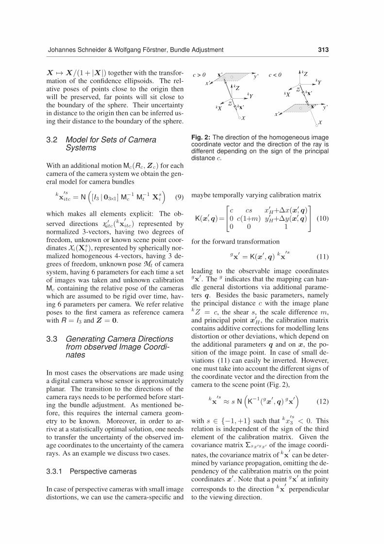
Fig. 2: The direction of the homogeneous imagecoordinate vector and the direction of the ray isdifferent depending on the sign of the principaldistance c.
maybe temporally varying calibration matrix
K(x′, q)=
⎡⎣c cs x′H+Δx(x′, q)
0 c(1+m) y′H+Δy(x′, q)0 0 1
⎤⎦ (10)
for the forward transformation
gx′= K(x′, q) kx
′s(11)
leading to the observable image coordinatesgx′
. The g indicates that the mapping can han-
dle general distortions via additional parame-
ters q. Besides the basic parameters, namely
the principal distance c with the image planekZ = c, the shear s, the scale difference m,
and principal point x′H , the calibration matrix
contains additive corrections for modelling lens
distortion or other deviations, which depend on
the additional parameters q and on x, the po-
sition of the image point. In case of small de-
viations (11) can easily be inverted. However,
one must take into account the different signs of
the coordinate vector and the direction from the
camera to the scene point (Fig. 2),
kx′s ≈ s N
(K−1(gx
′, q) gx
′)(12)
with s ∈ {−1,+1} such that kx′s3 < 0. This
relation is independent of the sign of the third
element of the calibration matrix. Given the
covariance matrix Σgx′gx′ of the image coordi-
nates, the covariance matrix of kx′can be deter-
mined by variance propagation, omitting the de-
pendency of the calibration matrix on the point
coordinates x′. Note that a point gx′at infinity
corresponds to the direction kx′
perpendicular
to the viewing direction.
314 Photogrammetrie • Fernerkundung • Geoinformation 4/2013
xk ’
xe xgr
- ’kx s
s
H
O
O
gφ
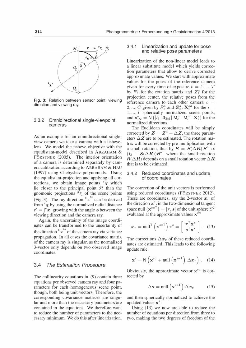
Fig. 3: Relation between sensor point, viewingdirection and viewing ray.
3.3.2 Omnidirectional single-viewpointcameras
As an example for an omnidirectional single-
view camera we take a camera with a fisheye-
lens. We model the fisheye objective with the
equidistant-model described in ABRAHAM &
FORSTNER (2005). The interior orientation
of a camera is determined separately by cam-
era calibration according to ABRAHAM & HAU
(1997) using Chebyshev polynomials. Using
the equidistant-projection and applying all cor-
rections, we obtain image points ex which
lie closer to the principal point H than the
gnomonic projections gx of the scene points
(Fig. 3). The ray direction kx′s
can be derived
from ex by using the normalized radial distance
r′ = |ex| growing with the angle φ between the
viewing direction and the camera ray.
Again, the uncertainty of the image coordi-
nates can be transformed to the uncertainty of
the direction kx′s
of the camera ray via variance
propagation. In all cases the covariance matrix
of the camera ray is singular, as the normalized
3-vector only depends on two observed image
coordinates.
3.4 The Estimation Procedure
The collinearity equations in (9) contain three
equations per observed camera ray and four pa-
rameters for each homogeneous scene point,
though, both being unit vectors. Therefore, the
corresponding covariance matrices are singu-
lar and more than the necessary parameters are
contained in the equations. We therefore want
to reduce the number of parameters to the nec-
essary minimum. We do this after linearization.
3.4.1 Linearization and update for poseand relative pose parameters
Linearization of the non-linear model leads to
a linear substitute model which yields correc-
tion parameters that allow to derive corrected
approximate values. We start with approximate
values for the poses of the reference camera
given for every time of exposure t = 1, ..., Tby Ra
t for the rotation matrix and Zat for the
projection center, the relative poses from the
reference camera to each other camera c =2, ..., C given by Ra
c and Zac , Xsa
i for the i =1, ..., I spherically normalized scene points,
and xaitc = N
([I3 |03×1] M−1
c M−1t Xs
i
)for the
normalized directions.
The Euclidean coordinates will be simply
corrected by Z = Za +ΔZ, the three param-
eters ΔZ are to be estimated. The rotation ma-
trix will be corrected by pre-multiplication with
a small rotation, thus by R = R(ΔR)Ra ≈(I3 + S(ΔR))Ra, where the small rotation
R(ΔR) depends on a small rotation vector ΔRthat is to be estimated.
3.4.2 Reduced coordinates and updateof coordinates
The correction of the unit vectors is performed
using reduced coordinates (FORSTNER 2012).
These are coordinates, say the 2-vector xr of
the direction xs, in the two-dimensional tangent
space null(xsaT
)= [r, s] of the unit sphere S2
evaluated at the approximate values xsa
xr = nullT(xsaT
)xs =
[rTxs
sTxs
]. (13)
The corrections Δxr of these reduced coordi-
nates are estimated. This leads to the following
update rule
xs = N(xsa + null
(xsaT
)Δxr
). (14)
Obviously, the approximate vector xsa is cor-
rected by
Δx = null
(xsaT
)Δxr (15)
and then spherically normalized to achieve the
updated values xs.
Using (13) we now are able to reduce the
number of equations per direction from three to
two, making the two degrees of freedom of the
Johannes Schneider & Wolfgang Forstner, Bundle Adjustment 315
observed direction explicit. This results in pre-
multiplication of all observation equations on
(9) with nullT(kx
saTitc
). Following (15) we use
the substitution ΔXsi = null
(XsaT
i
)ΔXr,i
when linearizing the scene coordinates. Then
we obtain the linearized model
kxr,itc + vxr,itc (16)
= JTRaTc RaT
t S(Xai0)ΔRt
−XaihJTRaT
c RaTt ΔZt
+ JTRaTc S
(RaT
t (Xai0−Xa
ihZat ))ΔRc
−XaihJT RaT
c ΔZt
+ JT[I3 |03](Mac )
−1(Mat )
−1null
(XaT
i
)ΔXri
with
J =1
|x|
(I3−
xxT
xTx
)null(xT)
∣∣∣∣x=kx
a
itc
(17)
and the partitioned homogeneous vector Xs =
[X0;Xh] depending on ΔRt, ΔZt, ΔRc,
ΔZc and ΔXr,i.
We now arrive at a well-defined optimization
problem: find ΔXr,i, ΔRt, ΔZt, ΔRc, ΔZc
minimizing
Ω(ΔXr,i, ΔRt, ΔZt, ΔRc, ΔZc
)(18)
=∑itc
vTr,itcΣ
−1xr,itcxr,itc
vr,itc
with the regular 2×2-covariance matrices
Σxr,itcxr,itc (19)
= kJT
s (kx
a
itc)
[Σxitcxitc 0
0T 0
]kJs(
kxa
itc) .
4 Experiments
4.1 Implementation Details
We have implemented the bundle adjustment as
a Gauss-Markov model in Matlab. Observa-
tions are bundles of rays, the interior orienta-
tions of all cameras of the camera system are
assumed to be known. To overcome the rank
deficiency we define the gauge by introducing
seven centroid constraints on the approximate
values of the scene points. This results in a free
bundle adjustment, where the trace of the co-
variance matrix of the estimated scene points
is minimal. We can robustify the cost function
by down-weighting measurements whose resid-
ual errors are too large by minimizing the robust
Huber cost function HUBER (1981).
For the initialization sufficiently accurate ap-
proximate values for the scene point coordi-
nates Xai and for the translation and the rota-
tion of the relative poses Mac of each camera in
the camera system of the reference camera as
well as for the poses Mat of the reference cam-
era in the scene coordinate system at the times
of synchronized exposure are needed. Firstly,
we determine the pose of each camera without
considering the cameras as a rigid multi-camera
rig using the bundle adjustment program Au-
relo provided by LABE & FORSTNER (2006).
With the first camera as the reference camera
we then determine approximate values for all
c = 2, ..., C relative poses Mac robustly using
the median quaternion and median translation
over all t = 1, ..., T unconstrained estimated
relative poses. Scene points are triangulated by
using all corresponding image points that are
consistent with the approximated relative poses
and the poses of the reference camera in the
scene coordinate system. Ray directions with
large residuals are discarded.
4.2 Test on Correctness andAdvantage
We first check the correctness of the imple-
mented model and then show the advantage of
including far points or points with glancing in-
tersections within the bundle adjustment based
on a simulated scenario.
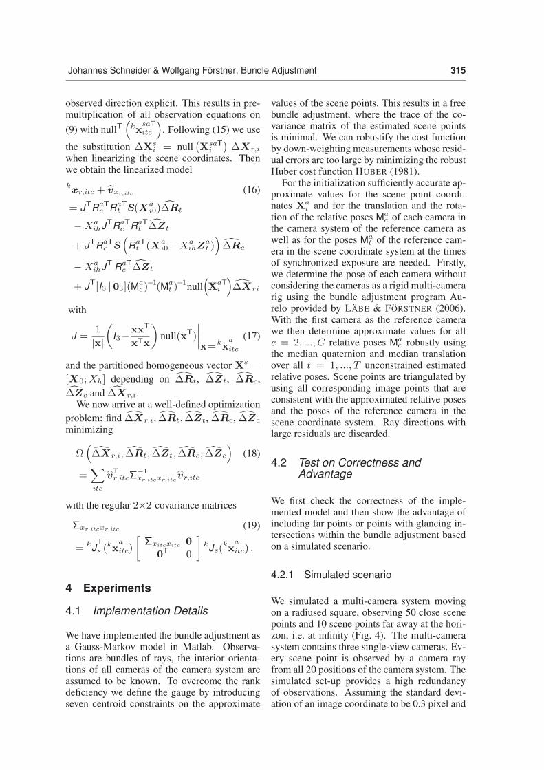
4.2.1 Simulated Scenario
We simulated a multi-camera system moving
on a radiused square, observing 50 close scene
points and 10 scene points far away at the hori-
zon, i.e. at infinity (Fig. 4). The multi-camera
system contains three single-view cameras. Ev-
ery scene point is observed by a camera ray
from all 20 positions of the camera system. The
simulated set-up provides a high redundancy
of observations. Assuming the standard devi-
ation of an image coordinate to be 0.3 pixel and
316 Photogrammetrie • Fernerkundung • Geoinformation 4/2013
−2 −1 0 1 2−2
−1.5
−1
−0.5
0
0.5
1
1.5
2
x−axis in meters
y−ax
is in
met
ers
Fig. 4: Simulation of a moving multi-camera sys-tem (poses of reference camera shown as boldtripods) with loop closing. Scene points nearby(crossed dots) and at the horizon (empty dots)being numerically at infinity are observed.
a principal distance of 500 pixel, we add nor-
mally distributed noise with σl = 0.3/500 ra-
diant on the spherically normalized camera rays
to simulate the observation process (Fig. 4). As
initial values for the bundle adjustment we ran-
domly disturb both the generated spherical nor-
malized homogeneous scene points Xsi , which
are directions, by 6◦, the generated motion pa-
rameters of the reference camera Rt and Zt of
Mt by 3◦ and 2 cm, and the relative pose pa-
rameters of the remaining cameras Rc and Zc
of Mc by 3◦ and 10 % of the relative distances
between the projection centres.
The iterative estimation procedure stops after
eight iterations, when the maximum normalized
observation update is less than 10−6. The resid-
uals of the observed image rays in the tangent
space of the adjusted camera rays, which are
approximate angles between the rays in radi-
ants, do not show any deviation from the normal
distribution. The estimated a posteriori vari-
ance factor σ20 = 0.99252 approves the a pri-
ori stochastic model with the variance factor
σ20 = 1. In order to test if the estimated ori-
entation parameters and scene point coordinates
represent the maximum likelihood estimates for
normally distributed noise of the observations,
we have generated the same simulation 2000
times with different random noise. The mean
of the estimated variance factors is not signif-
icantly different from one, indicating an unbi-
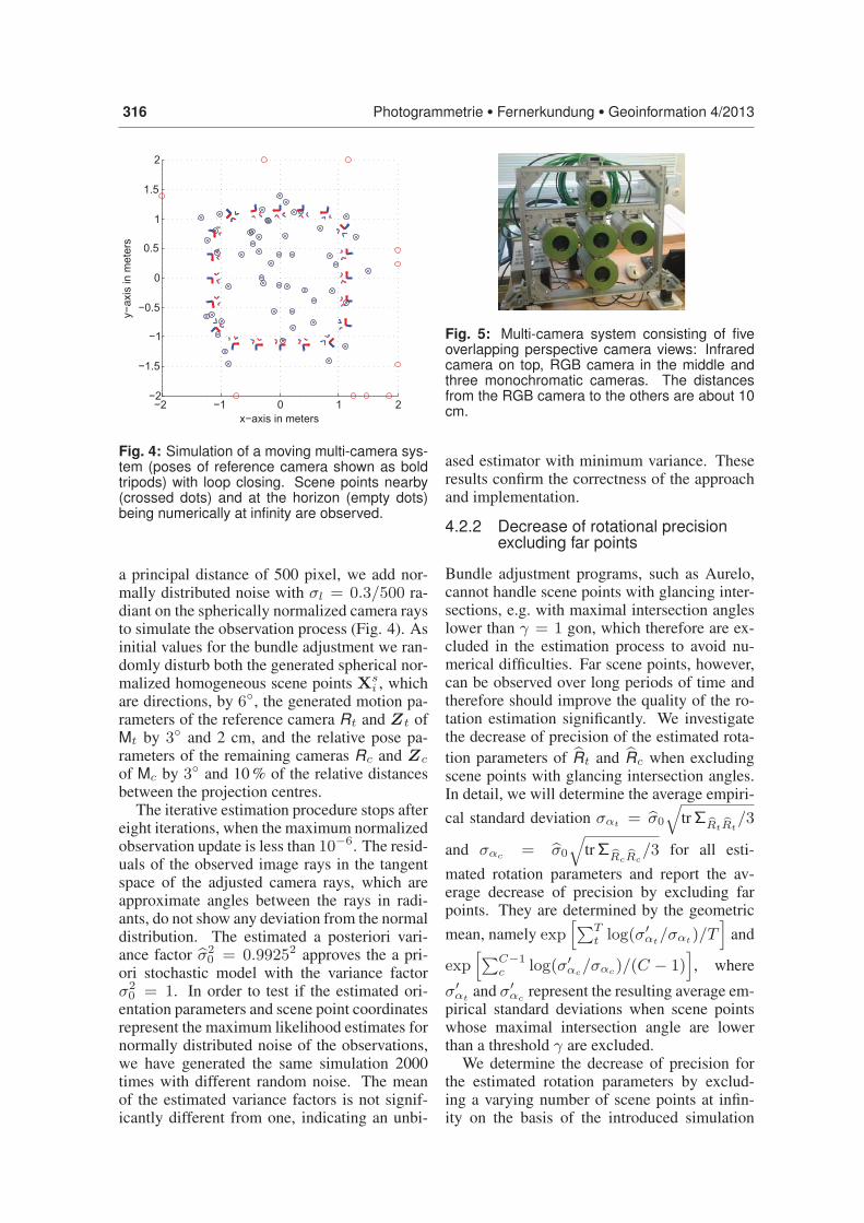
Fig. 5: Multi-camera system consisting of fiveoverlapping perspective camera views: Infraredcamera on top, RGB camera in the middle andthree monochromatic cameras. The distancesfrom the RGB camera to the others are about 10cm.
ased estimator with minimum variance. These
results confirm the correctness of the approach
and implementation.
4.2.2 Decrease of rotational precisionexcluding far points
Bundle adjustment programs, such as Aurelo,
cannot handle scene points with glancing inter-
sections, e.g. with maximal intersection angles
lower than γ = 1 gon, which therefore are ex-
cluded in the estimation process to avoid nu-
merical difficulties. Far scene points, however,
can be observed over long periods of time and
therefore should improve the quality of the ro-
tation estimation significantly. We investigate
the decrease of precision of the estimated rota-
tion parameters of Rt and Rc when excluding
scene points with glancing intersection angles.
In detail, we will determine the average empiri-
cal standard deviation σαt = σ0
√trΣ
RtRt/3
and σαc = σ0
√trΣ
RcRc/3 for all esti-
mated rotation parameters and report the av-
erage decrease of precision by excluding far
points. They are determined by the geometric
mean, namely exp[∑T
t log(σ′αt/σαt)/T
]and
exp[∑C−1
c log(σ′αc/σαc)/(C − 1)
], where
σ′αt
and σ′αc
represent the resulting average em-
pirical standard deviations when scene points
whose maximal intersection angle are lower
than a threshold γ are excluded.
We determine the decrease of precision for
the estimated rotation parameters by exclud-
ing a varying number of scene points at infin-
ity on the basis of the introduced simulation

Johannes Schneider & Wolfgang Forstner, Bundle Adjustment 317
Fig. 6: Left: Illustration of the estimated scene points and poses of the reference camera. The redline denotes the known length on a poster for scale definition. Right: The estimated relative poses.
of a moving multi-camera system. Again we
generate 50 scene points close to the multi-
camera positions and vary the number of scene
points at infinity to be 5, 10, 20, 50 and
100. The resulting average decrease in preci-
sion of the estimated rotations in Mc is 6.21 %,
8.98 %, 19.90 %, 42.29 % and 75.60 % and in
Mt 7.15 %, 11.77 %, 27.67 %, 54.56 % and
91.28 %, respectively. This strongly proves the
points at infinity to have a highly relevant posi-
tive influence on the rotational precision.
4.3 Calibration of Multi-CameraSystems
4.3.1 Calibration with overlapping views
We now describe the calibration of the camera
system shown in Fig. 5 with highly overlapping
views, which is used for 3D reconstruction of
vines. In order to determine the relative poses
of the multi-camera system we apply the bun-
dle adjustment to 100 images of a wall draped
with highly textured posters. The images were
taken at 20 stations in a synchronized way. We
use Aurelo without considering the known rel-
ative orientation between the cameras to ob-
tain an initial solution for each camera and the
scene points. The dataset contains 593,412 im-
age points and 63,140 observed scene points.
Starting from an a priori standard deviation
of the image coordinates of σl = 1 pixel, the
a posteriori variance factor is estimated with
σ20 = 0.112 indicating the automatically ex-
tracted Lowe points to have an average preci-
sion of approximately 0.1 pixel. This high pre-
cision of the point detection results mainly from
the good images and the calibration quality of
the camera used. Fig. 6 illustrates the estimated
scene points and poses as well as the estimated
relative poses.
The estimated uncertainty of the estimated
rotations of the cameras with regard to the ref-
erence camera is 0.1 mgrad – 0.2 mgrad around
the viewing direction axis and 0.4 mgrad –
0.8 mgrad orthogonal to it. We scale the pho-
togrammetric model by using a measured dis-
tance of 1.105 m with an error of about 0.1 %.
The uncertainty of the estimated relative trans-
lations is 0.02 mm – 0.04 mm in viewing direc-
tion and 0.1 mm – 0.2 mm orthogonal to it.
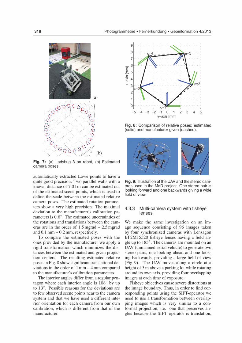
4.3.2 Multi-camera system Ladybug 3
The omnidirectional multi-camera system La-
dybug 3 consists of six cameras, five of which
are mounted in a circular manner, one show-
ing upwards, together covering 80 % of the
full viewing sphere. Neighbouring images only
have a very small overlap, which is too weak
for system calibration without additional in-
formation. We have mounted the omnidirec-
tional multi-camera system Ladybug 3 on a
robot (Fig. 7a), which executes a circular move-
ment with a radius of 50 cm in a highly textured
room while the Ladybug is taking synchronized
images. This ensures overlapping images of
different cameras at different times of the ex-
posure. Approximate values for this image se-
quence consisting of 150 images taken by the
five horizontal cameras at 30 exposure times
are obtained with Aurelo that provides 135,012
image points of 24,078 observed scene points.
The resulting 150 camera poses are shown in
Fig. 7b.
After applying our bundle adjustment the es-
timated a posteriori variance factor amounts to
σ20 = 0.252 using a priori stochastic model with
σl = 1 pixel for the image points, indicating the
318 Photogrammetrie • Fernerkundung • Geoinformation 4/2013
(a)
(b)
Fig. 7: (a) Ladybug 3 on robot, (b) Estimatedcamera poses.
automatically extracted Lowe points to have a
quite good precision. Two parallel walls with a
known distance of 7.01 m can be estimated out
of the estimated scene points, which is used to
define the scale between the estimated relative
camera poses. The estimated rotation parame-
ters show a very high precision. The maximal
deviation to the manufacturer’s calibration pa-
rameters is 0.6◦. The estimated uncertainties of
the rotations and translations between the cam-
eras are in the order of 1.5 mgrad – 2.5 mgrad
and 0.1 mm – 0.2 mm, respectively.
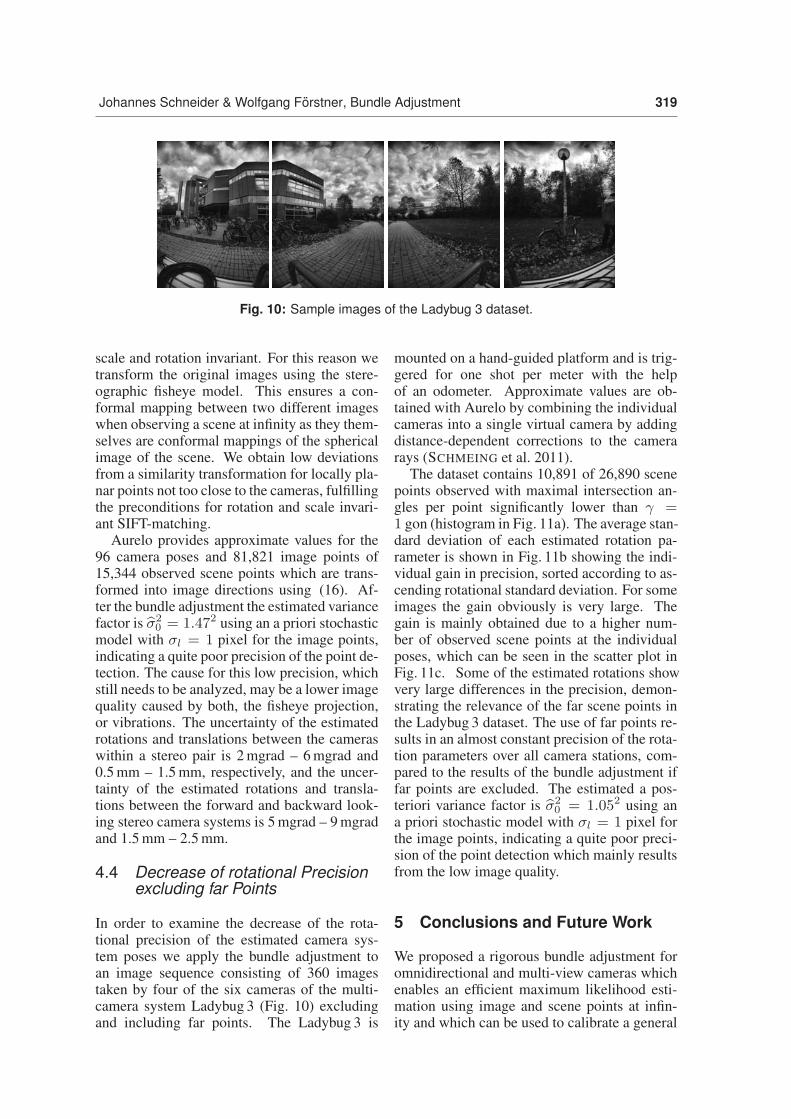
To compare the estimated poses with the
ones provided by the manufacturer we apply a
rigid transformation which minimizes the dis-
tances between the estimated and given projec-
tion centers. The resulting estimated relative
poses in Fig. 8 show significant translational de-
viations in the order of 1 mm – 4 mm compared
to the manufacturer’s calibration parameters.
The interior angles differ from a regular pen-
tagon where each interior angle is 108◦ by up
to 13◦. Possible reasons for the deviations are
to few observed scene points near to the camera
system and that we have used a different inte-
rior orientation for each camera from our own
calibration, which is different from that of the
manufacturer.
−5 −4 −3 −2 −1 0 1 2 3 4 5
0
1
2
3
4
5
6
7
8
9
y−axis [mm]
z−ax
is [m
m]
c=5c=2
c=3
c=1
c=4
Fig. 8: Comparison of relative poses: estimated(solid) and manufacturer given (dashed).
Fig. 9: Illustration of the UAV and the stereo cam-eras used in the MoD-project. One stereo pair islooking forward and one backwards giving a widefield of view.
4.3.3 Multi-camera system with fisheyelenses
We make the same investigation on an im-
age sequence consisting of 96 images taken
by four synchronized cameras with Lensagon
BF2M15520 fisheye lenses having a field an-
gle up to 185◦. The cameras are mounted on an
UAV (unmanned aerial vehicle) to generate two
stereo pairs, one looking ahead and one look-
ing backwards, providing a large field of view
(Fig. 9). The UAV moves along a circle at a
height of 5 m above a parking lot while rotating
around its own axis, providing four overlapping
images at each time of exposure.
Fisheye objectives cause severe distortions at
the image boundary. Thus, in order to find cor-
responding points using the SIFT-operator we
need to use a transformation between overlap-
ping images which is very similar to a con-
formal projection, i.e. one that preserves an-
gles because the SIFT operator is translation,
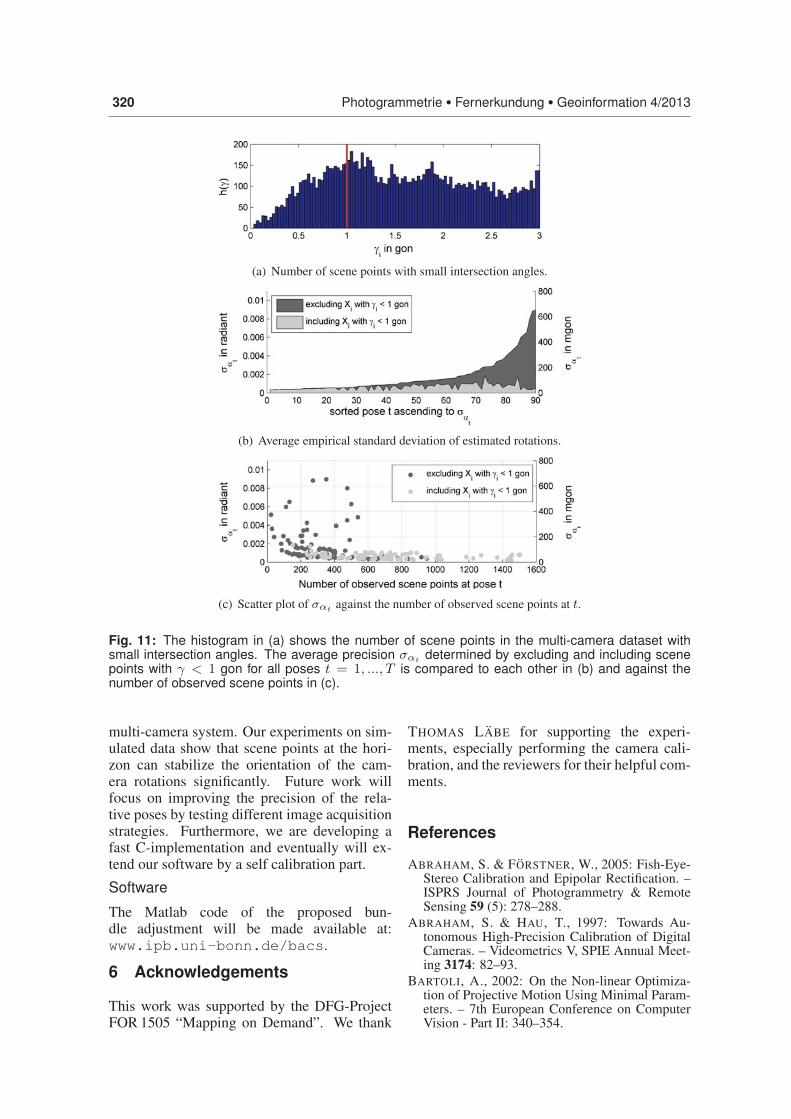
Johannes Schneider & Wolfgang Forstner, Bundle Adjustment 319
Fig. 10: Sample images of the Ladybug 3 dataset.
scale and rotation invariant. For this reason we
transform the original images using the stere-
ographic fisheye model. This ensures a con-
formal mapping between two different images
when observing a scene at infinity as they them-
selves are conformal mappings of the spherical
image of the scene. We obtain low deviations
from a similarity transformation for locally pla-
nar points not too close to the cameras, fulfilling
the preconditions for rotation and scale invari-
ant SIFT-matching.
Aurelo provides approximate values for the
96 camera poses and 81,821 image points of
15,344 observed scene points which are trans-
formed into image directions using (16). Af-
ter the bundle adjustment the estimated variance
factor is σ20 = 1.472 using an a priori stochastic
model with σl = 1 pixel for the image points,
indicating a quite poor precision of the point de-
tection. The cause for this low precision, which
still needs to be analyzed, may be a lower image
quality caused by both, the fisheye projection,
or vibrations. The uncertainty of the estimated
rotations and translations between the cameras
within a stereo pair is 2 mgrad – 6 mgrad and
0.5 mm – 1.5 mm, respectively, and the uncer-
tainty of the estimated rotations and transla-
tions between the forward and backward look-
ing stereo camera systems is 5 mgrad – 9 mgrad
and 1.5 mm – 2.5 mm.
4.4 Decrease of rotational Precisionexcluding far Points
In order to examine the decrease of the rota-
tional precision of the estimated camera sys-
tem poses we apply the bundle adjustment to
an image sequence consisting of 360 images
taken by four of the six cameras of the multi-
camera system Ladybug 3 (Fig. 10) excluding
and including far points. The Ladybug 3 is
mounted on a hand-guided platform and is trig-
gered for one shot per meter with the help
of an odometer. Approximate values are ob-
tained with Aurelo by combining the individual
cameras into a single virtual camera by adding
distance-dependent corrections to the camera
rays (SCHMEING et al. 2011).
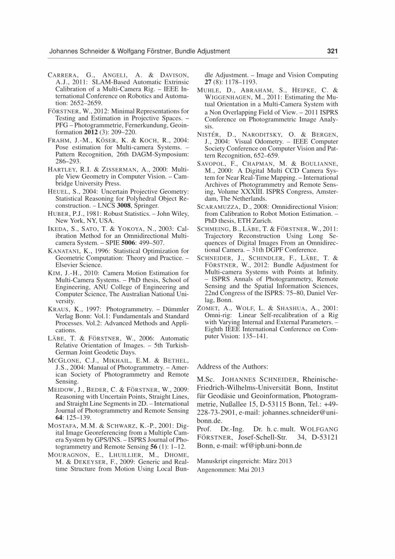
The dataset contains 10,891 of 26,890 scene
points observed with maximal intersection an-
gles per point significantly lower than γ =1 gon (histogram in Fig. 11a�. The average stan-
dard deviation of each estimated rotation pa-
rameter is shown in Fig. 11b showing the indi-
vidual gain in precision, sorted according to as-
cending rotational standard deviation. For some
images the gain obviously is very large. The
gain is mainly obtained due to a higher num-
ber of observed scene points at the individual
poses, which can be seen in the scatter plot in
Fig. 11c. Some of the estimated rotations show
very large differences in the precision, demon-
strating the relevance of the far scene points in
the Ladybug 3 dataset. The use of far points re-
sults in an almost constant precision of the rota-
tion parameters over all camera stations, com-
pared to the results of the bundle adjustment if
far points are excluded. The estimated a pos-
teriori variance factor is σ20 = 1.052 using an
a priori stochastic model with σl = 1 pixel for
the image points, indicating a quite poor preci-
sion of the point detection which mainly results
from the low image quality.
5 Conclusions and Future Work
We proposed a rigorous bundle adjustment for
omnidirectional and multi-view cameras which
enables an efficient maximum likelihood esti-
mation using image and scene points at infin-
ity and which can be used to calibrate a general
320 Photogrammetrie • Fernerkundung • Geoinformation 4/2013
(a) Number of scene points with small intersection angles.
(b) Average empirical standard deviation of estimated rotations.
(c) Scatter plot of σαt against the number of observed scene points at t.
Fig. 11: The histogram in (a) shows the number of scene points in the multi-camera dataset withsmall intersection angles. The average precision σαt determined by excluding and including scenepoints with γ < 1 gon for all poses t = 1, ..., T is compared to each other in (b) and against thenumber of observed scene points in (c).
multi-camera system. Our experiments on sim-
ulated data show that scene points at the hori-
zon can stabilize the orientation of the cam-
era rotations significantly. Future work will
focus on improving the precision of the rela-
tive poses by testing different image acquisition
strategies. Furthermore, we are developing a
fast C-implementation and eventually will ex-
tend our software by a self calibration part.
Software
The Matlab code of the proposed bun-
dle adjustment will be made available at:
www.ipb.uni-bonn.de/bacs.
6 Acknowledgements
This work was supported by the DFG-Project
FOR 1505 “Mapping on Demand”. We thank
THOMAS LABE for supporting the experi-
ments, especially performing the camera cali-
bration, and the reviewers for their helpful com-
ments.
References
ABRAHAM, S. & FORSTNER, W., 2005: Fish-Eye-Stereo Calibration and Epipolar Rectification. –ISPRS Journal of Photogrammetry & RemoteSensing 59 (5): 278–288.
ABRAHAM, S. & HAU, T., 1997: Towards Au-tonomous High-Precision Calibration of DigitalCameras. – Videometrics V, SPIE Annual Meet-ing 3174: 82–93.
BARTOLI, A., 2002: On the Non-linear Optimiza-tion of Projective Motion Using Minimal Param-eters. – 7th European Conference on ComputerVision - Part II: 340–354.
Johannes Schneider & Wolfgang Forstner, Bundle Adjustment 321
CARRERA, G., ANGELI, A. & DAVISON,A.J., 2011: SLAM-Based Automatic ExtrinsicCalibration of a Multi-Camera Rig. – IEEE In-ternational Conference on Robotics and Automa-tion: 2652–2659.
FORSTNER, W., 2012: Minimal Representations forTesting and Estimation in Projective Spaces. –PFG – Photogrammetrie, Fernerkundung, Geoin-formation 2012 (3): 209–220.
FRAHM, J.-M., KOSER, K. & KOCH, R., 2004:Pose estimation for Multi-camera Systems. –Pattern Recognition, 26th DAGM-Symposium:286–293.
HARTLEY, R.I. & ZISSERMAN, A., 2000: Multi-ple View Geometry in Computer Vision. – Cam-bridge University Press.
HEUEL, S., 2004: Uncertain Projective Geometry:Statistical Reasoning for Polyhedral Object Re-construction. – LNCS 3008, Springer.
HUBER, P.J., 1981: Robust Statistics. – John Wiley,New York, NY, USA.
IKEDA, S., SATO, T. & YOKOYA, N., 2003: Cal-ibration Method for an Omnidirectional Multi-camera System. – SPIE 5006: 499–507.
KANATANI, K., 1996: Statistical Optimization forGeometric Computation: Theory and Practice. –Elsevier Science.
KIM, J.-H., 2010: Camera Motion Estimation forMulti-Camera Systems. – PhD thesis, School ofEngineering, ANU College of Engineering andComputer Science, The Australian National Uni-versity.
KRAUS, K., 1997: Photogrammetry. – DummlerVerlag Bonn: Vol.1: Fundamentals and StandardProcesses. Vol.2: Advanced Methods and Appli-cations.
LABE, T. & FORSTNER, W., 2006: AutomaticRelative Orientation of Images. – 5th Turkish-German Joint Geodetic Days.
MCGLONE, C.J., MIKHAIL, E.M. & BETHEL,J.S., 2004: Manual of Photogrammetry. – Amer-ican Society of Photogrammetry and RemoteSensing.
MEIDOW, J., BEDER, C. & FORSTNER, W., 2009:Reasoning with Uncertain Points, Straight Lines,and Straight Line Segments in 2D. – InternationalJournal of Photogrammetry and Remote Sensing64: 125–139.
MOSTAFA, M.M. & SCHWARZ, K.-P., 2001: Dig-ital Image Georeferencing from a Multiple Cam-era System by GPS/INS. – ISPRS Journal of Pho-togrammetry and Remote Sensing 56 (1): 1–12.
MOURAGNON, E., LHUILLIER, M., DHOME,M. & DEKEYSER, F., 2009: Generic and Real-time Structure from Motion Using Local Bun-
dle Adjustment. – Image and Vision Computing27 (8): 1178–1193.
MUHLE, D., ABRAHAM, S., HEIPKE, C. &WIGGENHAGEN, M., 2011: Estimating the Mu-tual Orientation in a Multi-Camera System with
a Non Overlapping Field of View. – 2011 ISPRSConference on Photogrammetric Image Analy-sis.
NISTER, D., NARODITSKY, O. & BERGEN,J., 2004: Visual Odometry. – IEEE ComputerSociety Conference on Computer Vision and Pat-tern Recognition, 652–659.
SAVOPOL, F., CHAPMAN, M. & BOULIANNE,M., 2000: A Digital Multi CCD Camera Sys-tem for Near Real-Time Mapping. – InternationalArchives of Photogrammetry and Remote Sens-ing, Volume XXXIII. ISPRS Congress, Amster-dam, The Netherlands.
SCARAMUZZA, D., 2008: Omnidirectional Vision:from Calibration to Robot Motion Estimation. –PhD thesis, ETH Zurich.
SCHMEING, B., LABE, T. & FORSTNER, W., 2011:Trajectory Reconstruction Using Long Se-quences of Digital Images From an Omnidirec-tional Camera. – 31th DGPF Conference.
SCHNEIDER, J., SCHINDLER, F., LABE, T. &FORSTNER, W., 2012: Bundle Adjustment forMulti-camera Systems with Points at Infinity.– ISPRS Annals of Photogrammetry, RemoteSensing and the Spatial Information Sciences,22nd Congress of the ISPRS: 75–80, Daniel Ver-lag, Bonn.
ZOMET, A., WOLF, L. & SHASHUA, A., 2001:Omni-rig: Linear Self-recalibration of a Rigwith Varying Internal and External Parameters. –Eighth IEEE International Conference on Com-puter Vision: 135–141.
Address of the Authors:
M.Sc. JOHANNES SCHNEIDER, Rheinische-
Friedrich-Wilhelms-Universitat Bonn, Institut
fur Geodasie und Geoinformation, Photogram-
metrie, Nußallee 15, D-53115 Bonn, Tel.: +49-
228-73-2901, e-mail: johannes.schneider@uni-
bonn.de.
Prof. Dr.-Ing. Dr. h. c. mult. WOLFGANG
FORSTNER, Josef-Schell-Str. 34, D-53121
Bonn, e-mail: [email protected]
Manuskript eingereicht: Marz 2013
Angenommen: Mai 2013