
BULLETIN OF MONETARY ECONOMICS AND BANKING · Early Warning System and Currency Volatility...
133
Transcript of BULLETIN OF MONETARY ECONOMICS AND BANKING · Early Warning System and Currency Volatility...

BULLETIN OF MONETARY ECONOMICS AND BANKINGCentral Banking Research Department
Bank Indonesia
PatronBoard of Governors
Board of Editor
Prof. Dr. Anwar NasutionProf. Dr. Miranda S. Goeltom
Prof. Dr. InsukindroProf. Dr. Iwan Jaya Azis
Prof. Iftekhar HasanProf. Dr. Masaaki Komatsu
Dr. M. SyamsuddinDr. Perry Warjiyo
Dr. Iskandar Simorangkir Dr. Solikin M. JuhroDr. Haris Munandar
Dr. M. Edhie PurnawanDr. Burhanuddin Abdullah
Dr. Andi M. Alfian Parewangi
Editorial ChairmanDr. Perry Warjiyo
Managing EditorDr. Darsono
Dr. Siti AstiyahDr. Andi M. Alfian Parewangi
SecretariatIr. Triatmo Doriyanto, M.S
Nurhemi, S.E., M.ATri Subandoro, S.E
This bulletin is published by Bank Indonesia, Central Banking Research Department. Contents and results research in the writings in this bulletin entirely the responsibility of the authors and not an official view of Bank Indonesia.
We invite all parties to write in this bulletin paper delivered in the form files to Central Banking Research Department, Bank Indonesia, Tower Sjafruddin Prawiranegara Floor 21; Jl. M.H. Thamrin No. 2, Central Jakarta, email: [email protected].
The Bulletin is published quarterly in April, July, October and January,

Quarterly Outlook On Monetary, Banking, And Payment System In Indonesia:
Quarter III, 2016
TM. Arief Machmud, Syachman Perdymer, Muslimin Anwar,
Nurkholisoh Ibnu Aman, Tri Kurnia Ayu K,
Anggita Cinditya Mutiara K, Illinia Ayudhia Riyadi
Early Warning System and Currency Volatility Management In Emerging Market
Natasia Engeline S, Salomo Posmauli Matondang
The Impact of Geothermal Energy Sector Development on Electricity Sector
In Indonesia Economy
Nayasari Aissa, Djoni Hartono
Red Flags and Fraud Prevention on Rural Banks
Ni Wayan Rustiarini, Ni Nyoman Ayu Suryandari, I Kadek Satria Nova
Impact of Redenomination on Price, Volume, and Value of Transaction:
An Experimental Economic Approach
Danti Astrini, Bambang Juanda, Noer Azam Achsani
Volume 19, Number 2, October 2016
123
171
103
147
199
BULLETIN of moNETary EcoNomIcsaNd BaNkINg

This page intentionally left blank
103Quarterly Outlook On Monetary, Banking, and Payment System In Indonesia: Quarter III, 2016
TM. Arief Machmud, Syachman Perdymer, Muslimin Anwar, Nurkholisoh Ibnu Aman, Tri Kurnia Ayu K,
Anggita Cinditya Mutiara K, Illinia Ayudhia Riyadi1
1 Authors are researcher on Monetary and Economic Policy Department (DKEM). TM_Arief Machmud ([email protected]); Syachman Perdymer ([email protected]); Muslimin AAnwar ([email protected]); Nurkholisoh Ibnu Aman ([email protected]); Tri Kurnia Ayu K ([email protected]); Anggita Cinditya Mutiara K ([email protected]); Illinia Ayudhia Riyadi ([email protected]).
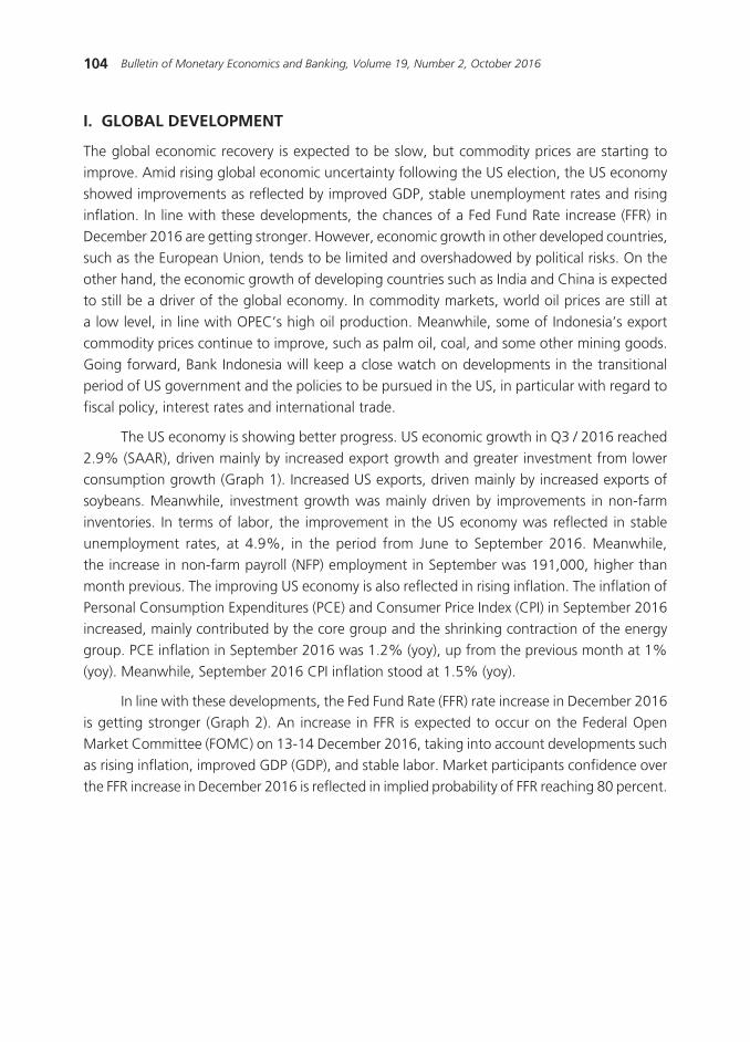
The growth of Indonesian economy on Quarter III, 2016 recorded positive growth with a well-
maintained financial system and macroeconomic stability. The economy grew moderately supported
by remaining strong domestic demand amidst the slow recovery of the global economy. The economic
stability is also good reflected on the low inflation, decreasing current account deficit, and relatively
stable exchange rate. An increase of domestic economy and lower global financial risk enable monetary
ease on Quarter III, 2016. Furthermore, the reduction of interest rate policy is well transmitted and is
expected to strengthen the growth momentum of the economy. Looking forward, Bank Indonesia will
keep strengthening his policy mix and macroprudential, and his coordination with the government to
ensure the inflation control, greater stimulus for growth, and the implementation of structural reform
run on the right track, and hence preserve the sustainable economic development.
Abstract
Keywords: Macroeconomy, Monetary, Economic Outlook
JEL Classification: C53, E66, F01, F41
QUARTERLY OUTLOOK ON MONETARY,BANKING, AND PAYMENT SYSTEM IN INDONESIA:
QUARTER III, 2016
104 Bulletin of Monetary Economics and Banking, Volume 19, Number 2, October 2016
I. GLOBAL DEVELOPMENT
The global economic recovery is expected to be slow, but commodity prices are starting to improve. Amid rising global economic uncertainty following the US election, the US economy showed improvements as reflected by improved GDP, stable unemployment rates and rising inflation. In line with these developments, the chances of a Fed Fund Rate increase (FFR) in December 2016 are getting stronger. However, economic growth in other developed countries, such as the European Union, tends to be limited and overshadowed by political risks. On the other hand, the economic growth of developing countries such as India and China is expected to still be a driver of the global economy. In commodity markets, world oil prices are still at a low level, in line with OPEC’s high oil production. Meanwhile, some of Indonesia’s export commodity prices continue to improve, such as palm oil, coal, and some other mining goods. Going forward, Bank Indonesia will keep a close watch on developments in the transitional period of US government and the policies to be pursued in the US, in particular with regard to fiscal policy, interest rates and international trade.
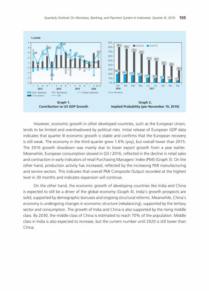
The US economy is showing better progress. US economic growth in Q3 / 2016 reached 2.9% (SAAR), driven mainly by increased export growth and greater investment from lower consumption growth (Graph 1). Increased US exports, driven mainly by increased exports of soybeans. Meanwhile, investment growth was mainly driven by improvements in non-farm inventories. In terms of labor, the improvement in the US economy was reflected in stable unemployment rates, at 4.9%, in the period from June to September 2016. Meanwhile, the increase in non-farm payroll (NFP) employment in September was 191,000, higher than month previous. The improving US economy is also reflected in rising inflation. The inflation of Personal Consumption Expenditures (PCE) and Consumer Price Index (CPI) in September 2016 increased, mainly contributed by the core group and the shrinking contraction of the energy group. PCE inflation in September 2016 was 1.2% (yoy), up from the previous month at 1% (yoy). Meanwhile, September 2016 CPI inflation stood at 1.5% (yoy).
In line with these developments, the Fed Fund Rate (FFR) rate increase in December 2016 is getting stronger (Graph 2). An increase in FFR is expected to occur on the Federal Open Market Committee (FOMC) on 13-14 December 2016, taking into account developments such as rising inflation, improved GDP (GDP), and stable labor. Market participants confidence over the FFR increase in December 2016 is reflected in implied probability of FFR reaching 80 percent.
105Quarterly Outlook On Monetary, Banking, and Payment System In Indonesia: Quarter III, 2016
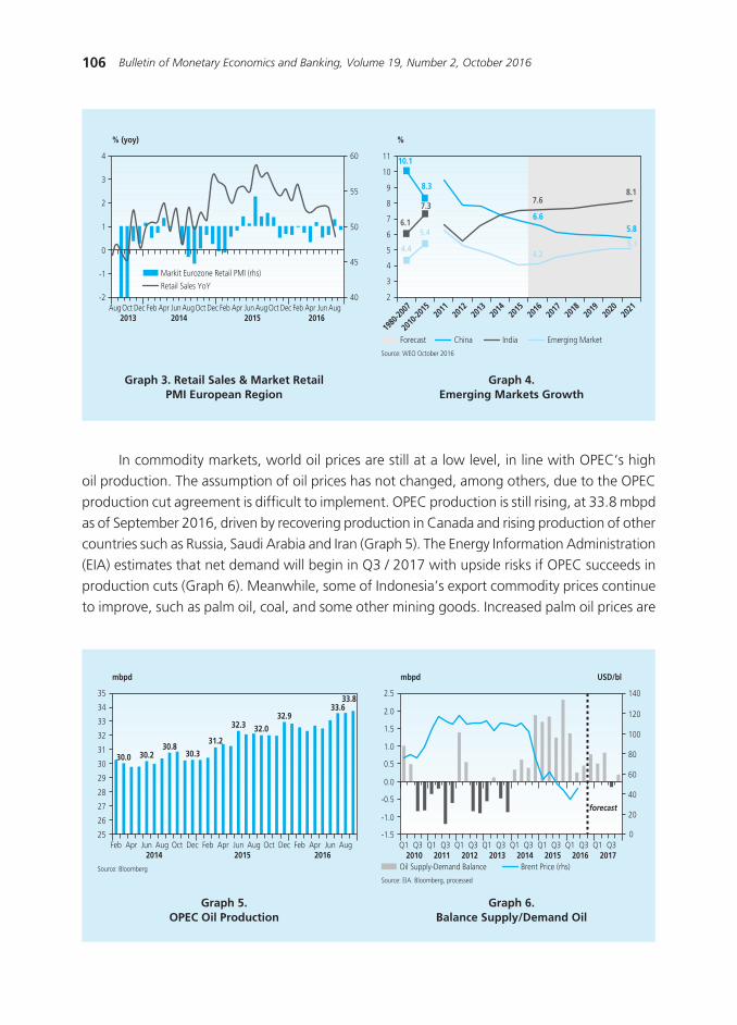
However, economic growth in other developed countries, such as the European Union, tends to be limited and overshadowed by political risks. Initial release of European GDP data indicates that quarter III economic growth is stable and confirms that the European recovery is still weak. The economy in the third quarter grew 1.6% (yoy), but overall lower than 2015. The 2016 growth slowdown was mainly due to lower export growth from a year earlier. Meanwhile, European consumption slowed in Q3 / 2016, reflected in the decline in retail sales and contraction in early indicators of retail Purchasing Managers’ Index (PMI) (Graph 3). On the other hand, production activity has increased, reflected by the increasing PMI manufacturing and service sectors. This indicates that overall PMI Composite Output recorded at the highest level in 30 months and indicates expansion will continue.
On the other hand, the economic growth of developing countries like India and China is expected to still be a driver of the global economy (Graph 4). India’s growth prospects are solid, supported by demographic bonuses and ongoing structural reforms. Meanwhile, China’s economy is undergoing changes in economic structure (rebalancing), supported by the tertiary sector and consumption. The growth of India and China is also supported by the rising middle class. By 2030, the middle class of China is estimated to reach 70% of the population. Middle class in India is also expected to increase, but the current number until 2020 is still lower than China.
Graph 1.Contribution to US GDP Growth
Graph 2.Implied Probability (per November 10, 2016)
2.8
0.8
3.1
-1.2
4.0 4.0
2.1
2.0
2.6
2.0
0.9
0.8
1.4
2.9
5.0
Govt. SpendingConsumption
Net ExportsGDP
Private Investment
��
���
���
���
���
���
���
���
���
���
��� ��� �� ��� � �� ��� ��� ������� ����
�������� ��������
������ ��� ���
��� ��� �� ����
������
������
��� ���
��� ���
���
�� ����������� �
106 Bulletin of Monetary Economics and Banking, Volume 19, Number 2, October 2016
In commodity markets, world oil prices are still at a low level, in line with OPEC’s high oil production. The assumption of oil prices has not changed, among others, due to the OPEC production cut agreement is difficult to implement. OPEC production is still rising, at 33.8 mbpd as of September 2016, driven by recovering production in Canada and rising production of other countries such as Russia, Saudi Arabia and Iran (Graph 5). The Energy Information Administration (EIA) estimates that net demand will begin in Q3 / 2017 with upside risks if OPEC succeeds in production cuts (Graph 6). Meanwhile, some of Indonesia’s export commodity prices continue to improve, such as palm oil, coal, and some other mining goods. Increased palm oil prices are
Graph 3. Retail Sales & Market RetailPMI European Region
Graph 5.OPEC Oil Production
Graph 4.Emerging Markets Growth
Graph 6.Balance Supply/Demand Oil
�������
��
��
�
�
�
�
� ��
��
��
��
�������� ��� ��� � � �������� ��� ��� � � �������� ��� ��� � � �����
���� ���� ���� ����
���������������������������� ���������������
�������
��
�������
������
����
����
����
����
����
����
����
����
����
����
�
�
�
�
�
�
�
�
�
��
�� ����
���
���
������
���
���
���
���
���
���
���
�������� ��� ��� ��������������
������������������������
����
��
��
��
��
��
��
��
��
��
��
��
���� ��������
��������
���� ��������
��������
��� ��� �� ��� � �� ��� ��� �� ��� � �� ��� ��� �� ������� ���� ����
����������������
���
���
���
���
���
���
����
����
����
���� ������
�
���
���
���
��
��
��
��
�� �� �� �� �� �� �� �� �� �� �� �� �� �� �� ������ ���� ���� ���� ���� ���� ���� ����
��������
��������� ����������� �����������������
��������� ���������������������
107Quarterly Outlook On Monetary, Banking, and Payment System In Indonesia: Quarter III, 2016
driven by production still disturbed due to El Nino (dry drought) and La Nina (wet drought). On the other hand, coal prices also increased due to increased demand for Chinese coal as steel production increased.
II. MACRO ECONOMIC DYNAMICS OF INDONESIA
2.1. Economic Growth
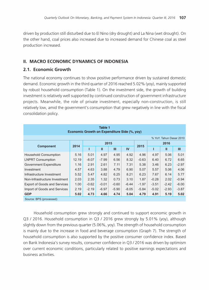
The national economy continues to show positive performance driven by sustained domestic demand. Economic growth in the third quarter of 2016 reached 5.02% (yoy), mainly supported by robust household consumption (Table 1). On the investment side, the growth of building investment is relatively well supported by continued construction of government infrastructure projects. Meanwhile, the role of private investment, especially non-construction, is still relatively low, amid the government’s consumption that grew negatively in line with the fiscal consolidation policy.
��������������������������� ���������������������
����
�����������������������
�������� ����
� �� ��� �� � �� ������������
���������� �������������� ����������������������������������������������������������������������������������������������������������������������������������������
�� �� � � ������������ ����� �� ��
��� �������� ������������������ �� ��
����������� �������� ������� ����� ��
�������� ��������������������� ��
����������� ������ �� ����������� ��
������������������ ���� ��������� �
�������������������������� ������ �
������������� ���������������� �
��� ����������������������������� ��
��������������������� �
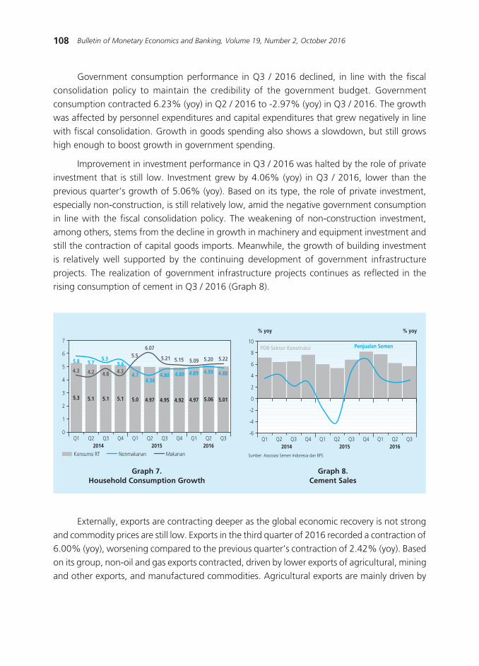
Household consumption grew strongly and continued to support economic growth in Q3 / 2016. Household consumption in Q3 / 2016 grew strongly by 5.01% (yoy), although slightly down from the previous quarter (5.06%, yoy). The strength of household consumption is mainly due to the increase in food and beverage consumption (Graph 7). The strength of household consumption is also supported by the positive consumer confidence index. Based on Bank Indonesia’s survey results, consumer confidence in Q3 / 2016 was driven by optimism over current economic conditions, particularly related to positive earnings expectations and business activities.
108 Bulletin of Monetary Economics and Banking, Volume 19, Number 2, October 2016
Graph 7.Household Consumption Growth
Graph 8.Cement Sales
Government consumption performance in Q3 / 2016 declined, in line with the fiscal consolidation policy to maintain the credibility of the government budget. Government consumption contracted 6.23% (yoy) in Q2 / 2016 to -2.97% (yoy) in Q3 / 2016. The growth was affected by personnel expenditures and capital expenditures that grew negatively in line with fiscal consolidation. Growth in goods spending also shows a slowdown, but still grows high enough to boost growth in government spending.
Improvement in investment performance in Q3 / 2016 was halted by the role of private investment that is still low. Investment grew by 4.06% (yoy) in Q3 / 2016, lower than the previous quarter’s growth of 5.06% (yoy). Based on its type, the role of private investment, especially non-construction, is still relatively low, amid the negative government consumption in line with the fiscal consolidation policy. The weakening of non-construction investment, among others, stems from the decline in growth in machinery and equipment investment and still the contraction of capital goods imports. Meanwhile, the growth of building investment is relatively well supported by the continuing development of government infrastructure projects. The realization of government infrastructure projects continues as reflected in the rising consumption of cement in Q3 / 2016 (Graph 8).
��� ������
���
�������
���� ���� ���� ���� ������� ��� ��� ���
�������
���� ���� ���� ���� ����
��� ��� ��� ��� ��� ���� ���� ���� ���� ���� ����
�
�
�
�
�
�
�
��� �� ���� �� �� �� �� �� �� ��
���� ���� �������������� ��������� �����
��������������������� ������������ ��
����� �����
��
�
�
�
�
�
��
��
���� �� �� �� �� �� �� �� �� �� ��
�� �� ��
��������� � � ����������� �������
Externally, exports are contracting deeper as the global economic recovery is not strong and commodity prices are still low. Exports in the third quarter of 2016 recorded a contraction of 6.00% (yoy), worsening compared to the previous quarter’s contraction of 2.42% (yoy). Based on its group, non-oil and gas exports contracted, driven by lower exports of agricultural, mining and other exports, and manufactured commodities. Agricultural exports are mainly driven by
109Quarterly Outlook On Monetary, Banking, and Payment System In Indonesia: Quarter III, 2016
contraction in food exports, especially CPO. Meanwhile, manufacturing exports also contracted due to sharp contraction in clothing exports along with declining exports to America. From the oil and gas group, export contraction is influenced by the policy to meet domestic gas needs.
In line with weakening exports and domestic demand, imports also contracted in Q3 / 2016. Imports contracted by 3.87% (yoy) in Q3 / 2016, larger than the previous quarter which contracted 2.93% (yoy). The import contraction was mainly due to the contraction of non-oil and gas imports. Based on the group, the weakening performance of non-oil and gas imports was mainly driven by the contraction in imports of capital goods, especially in the capital goods category, except for transportation equipment.
From the sectoral side, the industrial, agricultural and trade sectors are still growing positively. The industrial sector is still growing positively as reflected by the PMI indicator that is still at expansion level. The positive industrial sector is sourced from food and beverages sub-sector which is performing better performance driven by increasing number of tourists. Meanwhile, the mining sector grew positively for the first time since 2015 with an increase in the performance of the metal ore subsector as an improvement motor. The transportation and communications information sector also grew better than the previous quarter driven by the air transport subsector, along with the addition of new domestic and international flight routes.
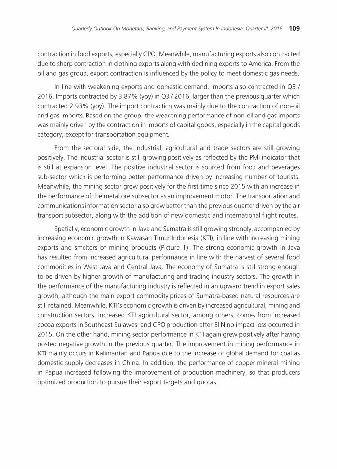
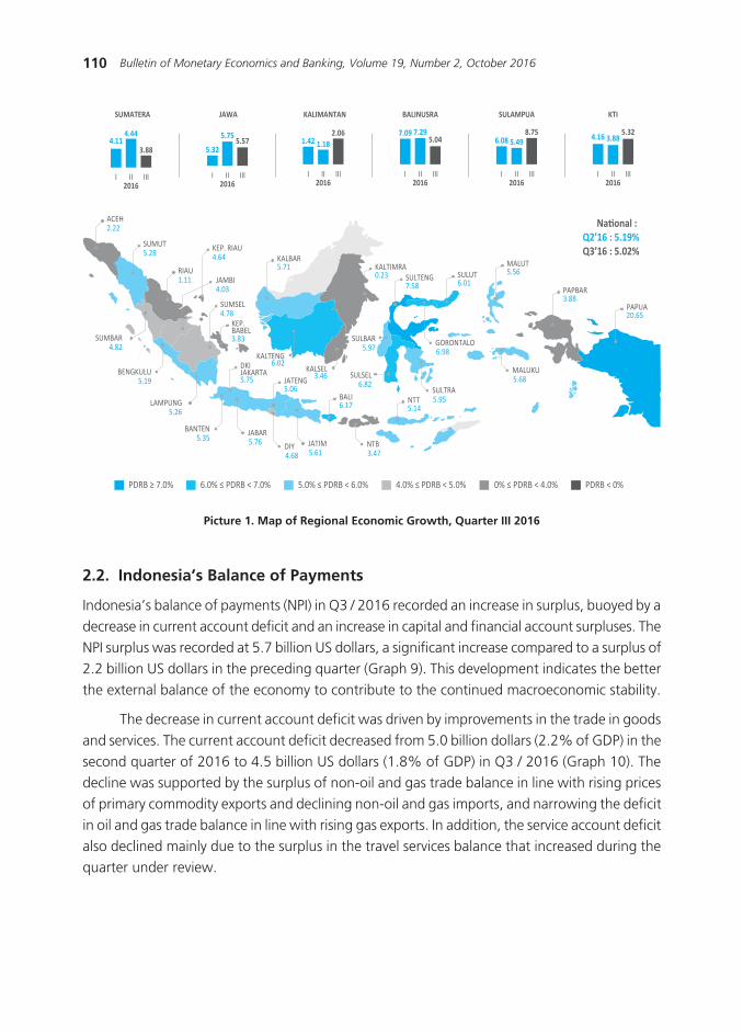
Spatially, economic growth in Java and Sumatra is still growing strongly, accompanied by increasing economic growth in Kawasan Timur Indonesia (KTI), in line with increasing mining exports and smelters of mining products (Picture 1). The strong economic growth in Java has resulted from increased agricultural performance in line with the harvest of several food commodities in West Java and Central Java. The economy of Sumatra is still strong enough to be driven by higher growth of manufacturing and trading industry sectors. The growth in the performance of the manufacturing industry is reflected in an upward trend in export sales growth, although the main export commodity prices of Sumatra-based natural resources are still retained. Meanwhile, KTI’s economic growth is driven by increased agricultural, mining and construction sectors. Increased KTI agricultural sector, among others, comes from increased cocoa exports in Southeast Sulawesi and CPO production after El Nino impact loss occurred in 2015. On the other hand, mining sector performance in KTI again grew positively after having posted negative growth in the previous quarter. The improvement in mining performance in KTI mainly occurs in Kalimantan and Papua due to the increase of global demand for coal as domestic supply decreases in China. In addition, the performance of copper mineral mining in Papua increased following the improvement of production machinery, so that producers optimized production to pursue their export targets and quotas.
110 Bulletin of Monetary Economics and Banking, Volume 19, Number 2, October 2016
2.2. Indonesia’s Balance of Payments
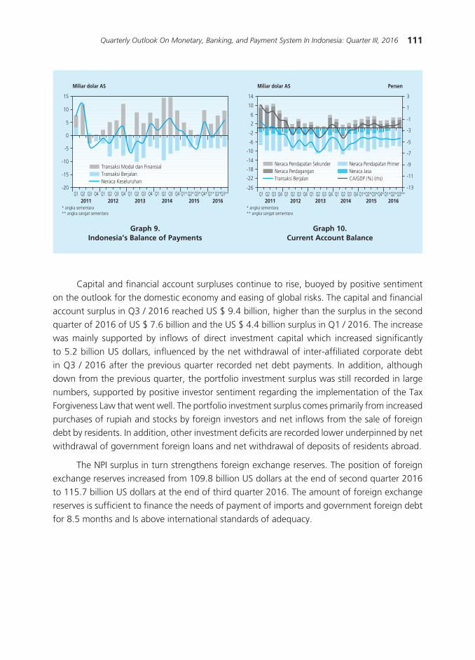
Indonesia’s balance of payments (NPI) in Q3 / 2016 recorded an increase in surplus, buoyed by a decrease in current account deficit and an increase in capital and financial account surpluses. The NPI surplus was recorded at 5.7 billion US dollars, a significant increase compared to a surplus of 2.2 billion US dollars in the preceding quarter (Graph 9). This development indicates the better the external balance of the economy to contribute to the continued macroeconomic stability.
The decrease in current account deficit was driven by improvements in the trade in goods and services. The current account deficit decreased from 5.0 billion dollars (2.2% of GDP) in the second quarter of 2016 to 4.5 billion US dollars (1.8% of GDP) in Q3 / 2016 (Graph 10). The decline was supported by the surplus of non-oil and gas trade balance in line with rising prices of primary commodity exports and declining non-oil and gas imports, and narrowing the deficit in oil and gas trade balance in line with rising gas exports. In addition, the service account deficit also declined mainly due to the surplus in the travel services balance that increased during the quarter under review.
Picture 1. Map of Regional Economic Growth, Quarter III 2016
PDRB ≥ 7.0% 5.0% ≤ PDRB < 6.0% 4.0% ≤ PDRB < 5.0% PDRB < 0%6.0% ≤ PDRB < 7.0% 0% ≤ PDRB < 4.0%
ACEH2.22
SUMUT5.28
RIAU1.11
KEP. BABEL3.83
DKI JAKARTA5.75 JATENG
5.06
SULTENG7.58
KALTIMRA0.23
KALBAR5.71
SULUT6.01
MALUT5.56
PAPBAR3.88
PAPUA20.65
BALI6.17 NTT
5.14
KEP. RIAU4.64
LAMPUNG5.26
BENGKULU5.19
BANTEN5.35
SULSEL6.82
SULBAR5.97
JABAR5.76 JATIM
5.61NTB3.47
KALTENG6.02
KALSEL3.46
GORONTALO6.98
MALUKU5.68
SULTRA5.95
SUMSEL4.78
JAMBI4.03
National : Q2’16 : 5.19%Q3’16 : 5.02%
DIY4.68
SUMBAR4.82
KALIMANTAN
I II III2016
1.42 1.182.06
BALINUSRA
I II III2016
7.09 7.295.04
SULAMPUA
I II III2016
6.08 5.498.75
KTI
I II III2016
4.16 3.885.32
JAWA
I II III2016
5.32
5.75 5.57
SUMATERA
I II III2016
4.114.44
3.88
111Quarterly Outlook On Monetary, Banking, and Payment System In Indonesia: Quarter III, 2016
Graph 9.Indonesia’s Balance of Payments
Graph 10.Current Account Balance
Capital and financial account surpluses continue to rise, buoyed by positive sentiment on the outlook for the domestic economy and easing of global risks. The capital and financial account surplus in Q3 / 2016 reached US $ 9.4 billion, higher than the surplus in the second quarter of 2016 of US $ 7.6 billion and the US $ 4.4 billion surplus in Q1 / 2016. The increase was mainly supported by inflows of direct investment capital which increased significantly to 5.2 billion US dollars, influenced by the net withdrawal of inter-affiliated corporate debt in Q3 / 2016 after the previous quarter recorded net debt payments. In addition, although down from the previous quarter, the portfolio investment surplus was still recorded in large numbers, supported by positive investor sentiment regarding the implementation of the Tax Forgiveness Law that went well. The portfolio investment surplus comes primarily from increased purchases of rupiah and stocks by foreign investors and net inflows from the sale of foreign debt by residents. In addition, other investment deficits are recorded lower underpinned by net withdrawal of government foreign loans and net withdrawal of deposits of residents abroad.
The NPI surplus in turn strengthens foreign exchange reserves. The position of foreign exchange reserves increased from 109.8 billion US dollars at the end of second quarter 2016 to 115.7 billion US dollars at the end of third quarter 2016. The amount of foreign exchange reserves is sufficient to finance the needs of payment of imports and government foreign debt for 8.5 months and Is above international standards of adequacy.
���
���
���
��
�
�
��
��
�� �� �� �� �� �� �� �� �� �� �� �� �� �� �� �� ��� ������������ ����������� ���� ���� ���� ���� ����
����������� ���������������������������������������������������
���������������
������������������������������������������
�� �� �� �� �� �� �� �� �� �� �� �� �� �� �� �� �������������������������� ���� ���� ���� ���� ����
��
��
�
�
��
��
���
���
���
���
���
�
�
��
��
��
��
��
���
���
��������������� � �� �
������ �������� ������������� ������������������� ��������
������ �������� ������������ ����� ��� ��� �����
� ����� ����������� ����� ������ ���������
112 Bulletin of Monetary Economics and Banking, Volume 19, Number 2, October 2016
2.3. Rupiah Exchange Rate
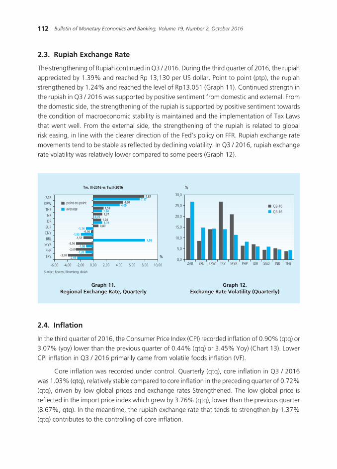
The strengthening of Rupiah continued in Q3 / 2016. During the third quarter of 2016, the rupiah appreciated by 1.39% and reached Rp 13,130 per US dollar. Point to point (ptp), the rupiah strengthened by 1.24% and reached the level of Rp13.051 (Graph 11). Continued strength in the rupiah in Q3 / 2016 was supported by positive sentiment from domestic and external. From the domestic side, the strengthening of the rupiah is supported by positive sentiment towards the condition of macroeconomic stability is maintained and the implementation of Tax Laws that went well. From the external side, the strengthening of the rupiah is related to global risk easing, in line with the clearer direction of the Fed’s policy on FFR. Rupiah exchange rate movements tend to be stable as reflected by declining volatility. In Q3 / 2016, rupiah exchange rate volatility was relatively lower compared to some peers (Graph 12).
Graph 11.Regional Exchange Rate, Quarterly
Graph 12.Exchange Rate Volatility (Quarterly)
����
����
����
����
����
����
����
����
����
����
����
����
����������
����������
����������
����������
����������
��������������
�������
������
�� ���������� ��
���������
����� ����� ����� ���� ���� ���� ���� ���� �����
�
� ������� ������ ���������������
������������� ������������
����
����
����
����
����
���
���
�
����������
��� ��� ��� ��� �� ��� � �� �� ���
2.4. Inflation
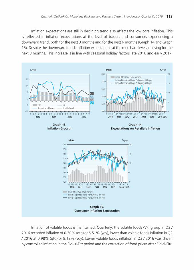
In the third quarter of 2016, the Consumer Price Index (CPI) recorded inflation of 0.90% (qtq) or 3.07% (yoy) lower than the previous quarter of 0.44% (qtq) or 3.45% Yoy) (Chart 13). Lower CPI inflation in Q3 / 2016 primarily came from volatile foods inflation (VF).
Core inflation was recorded under control. Quarterly (qtq), core inflation in Q3 / 2016 was 1.03% (qtq), relatively stable compared to core inflation in the preceding quarter of 0.72% (qtq), driven by low global prices and exchange rates Strengthened. The low global price is reflected in the import price index which grew by 3.76% (qtq), lower than the previous quarter (8.67%, qtq). In the meantime, the rupiah exchange rate that tends to strengthen by 1.37% (qtq) contributes to the controlling of core inflation.
113Quarterly Outlook On Monetary, Banking, and Payment System In Indonesia: Quarter III, 2016
Inflation expectations are still in declining trend also affects the low core inflation. This is reflected in inflation expectations at the level of traders and consumers experiencing a downward trend, both for the next 3 months and for the next 6 months (Graph 14 and Graph 15). Despite the downward trend, inflation expectations at the merchant level are rising for the next 3 months. This increase is in line with seasonal holiday factors late 2016 and early 2017.
Graph 13.Inflation Growth
Graph 14.Expectations on Retailers Inflation
Graph 15.Consumer Inflation Expectation
� � � � � �� � � � � � �� � � � � � �� � � � � ����� ���� ���� ����
���
��
�
�
��
��
�����
��� ������ ������������� ������������
����
����
����
�����
���
���
���
���
���
���
������
��
��
��
�
�
�����
� � � � ���� � � � ���� � � � ���� � � � ���� � � � ���� � � � ���� � � � �������� ���� ���� ���� ���� ���� ���� ����
��������� ������������������������������������� ���������������������������������������� �����������������������
���
���
���
���
���
���
���
���
���
��
��
��
�
�� � � � ���� � � � ���� � � � ���� � � � ���� � � � ���� � � � ���� � � � ���� �
���� ���� ���� ���� ���� ���� ���� ����
��������� ������������������������������������� ��������������������������������������� ����������������������
������ �����
Inflation of volatile foods is maintained. Quarterly, the volatile foods (VF) group in Q3 / 2016 recorded inflation of 0.30% (qtq) or 6.51% (yoy), lower than volatile foods inflation in Q2 / 2016 at 0.98% (qtq) or 8.12% (yoy). Lower volatile foods inflation in Q3 / 2016 was driven by controlled inflation in the Eid-ul-Fitr period and the correction of food prices after Eid al-Fitr.
114 Bulletin of Monetary Economics and Banking, Volume 19, Number 2, October 2016
Administered Prices Group (AP) in Q3 / 2016 recorded inflation, after two previous quarterly deflation. AP inflation was recorded at 0.93% (qtq) or an annual deflation of 0.38% (yoy), higher than the second quarter of 2016 which recorded a deflation of 0.73% (qtq) or 0.50% (yoy). Inflation in the AP group was mainly driven by the rise in electricity, cigarette and drinking water tariffs. Meanwhile, deflation occurred in inter-city transportation tariff and sea freight driven by post-Eid al-Fitr correction.
III. MONETARY DEVELOPMENT, BANKING AND PAYMENT SYSTEM
3.1. Monetary
Transmission of monetary policy easing through the interest rate channel continued in Q3 / 2016. Bank Indonesia lowered the BI 7-day Reverse Repo Rate (BI 7-day RR Rate) in September 2016 by 25 bps to 5.00%, followed by lower interest rates Deposit Facility (DF) to 4.25% and Lending Facility (LF) to 5.75%. The decline was followed by a decrease in the overnight interbank rate in both the O / N tenor and the longer tenor.
Liquidity conditions in the money market remain intact, despite pressure. The overnight interbank rates in Q3 / 2016 fell from 4.88% in Q2 / 2016 to 4.76% in Q3 / 2016. BI 7-day RR Rate Implementation replaced the BI Rate on August 19, 2016 and the policy of interest rate reduction The September 2016 policy also helped to push down the short tenor interest rate. However, the decline was not followed by the tenor of PUAB over 1 month which tended to increase. The condition of liquidity slightly under pressure in Q3 / 2016 was reflected in the average volume of overnight interbank money market and Deposit Facility (DF) which fell to Rp7.56 trillion and Rp63.7 trillion from the previous quarter Rp8.06 trillion and Rp64, 01 trillion. On the other hand, the average spread on overnight inter-market P / A interest rates increased from 23 bps in Q2 / 2016 to 32 bps in Q3 / 2016. The increase in the overnight interbank spread was influenced by the government’s lack of optimum spending, while the contraction of the Government continued to increase Related to tax revenue in line with the deadline for the implementation of the Phase I Amnesty program on September 30, 2016.
In line with the stance of monetary policy easing, bank deposit rates fell. Compared to second quarter of 2016, the weighted average (RRT) of deposit rates in Q3 / 2016 fell by 8 bps to 6.86%. Thus, on a year-to-date basis (ytd), the weighted average of time deposit rates in Q3 / 2016 had dropped by 108 bps. The decline in deposit rates occurred in all tenors. The biggest decline occurred in the 24-month tenor, which decreased by 148 bps (qtq) to 7.68% followed by the 6-month tenor, which fell by 43 bps (qtq) to 7.31%. The smallest decline occurred in short tenor 3 and 12 months which only decreased by 16 bps (qtq) to 6.84% and 7.60% respectively.
In line with the deposit interest rate, bank lending rates in Q3 / 2016 also fell. Compared to second quarter 2016, lending rates in quarter III 2016 fell by 15 bps to 12.23%. Year to date
115Quarterly Outlook On Monetary, Banking, and Payment System In Indonesia: Quarter III, 2016
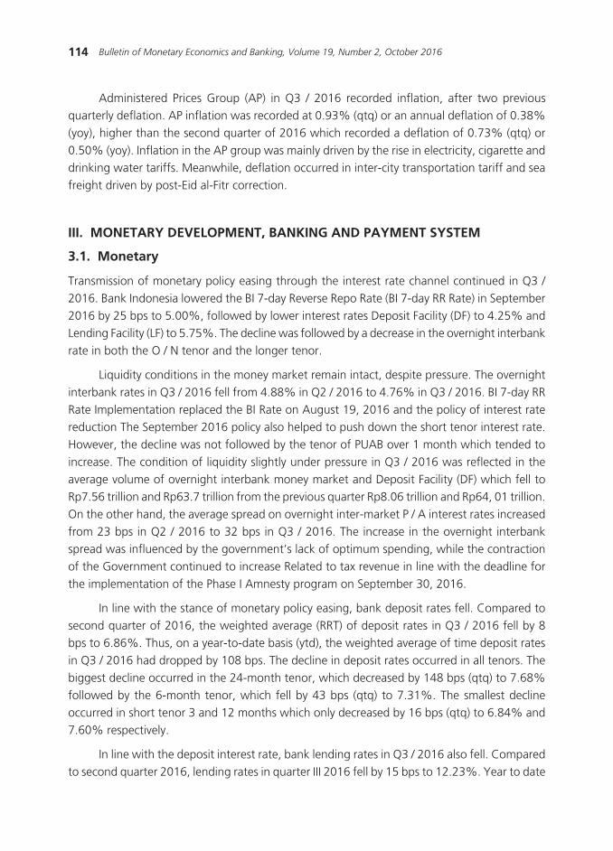
(ytd), lending rates in Q3 / 2016 fell by 60 bps, slower than the decline in RRT deposit rates. The decline in loan interest rates occurred in all types of loans, primarily in productive loans, with the largest decrease in interest rates on working capital credit (KMK), which fell 23 bps (qtq) to 11.59%, followed by a decrease in interest rates on Investment Credit (KI) By 13 bps (qtq) to 11.36% (Graph 16). In ytd, KMK and KI fell by 87 bps and 76 bps greater than KK which fell by 16 bps. The spread between deposit rates and lending rates in Q3 / 2016 increased 13 bps from the previous quarter to 537 bps (Graph 17).
Graph 16.Loan Interest Rate: KMK, KI dan KK
Graph 17.Spread of Interest Rate of Banking
����
����
����
����
����
����
����
����
�
�����
�����
����������
��� ������ ��� ��� �� ��� ������ ��� ��� �� ��� ������ ��� ��� �� ��� ������ ��� ������� ���� ���� ����
���������
����� ����
���� �����������
����
����
����
����
���
���
���
���
���
� �
���
���
���
���
���
���
���
������ ������ � � ���� ��� ������ � � ���� ��� ������ � � ���� ��� ������ � � ��
�������� ���� ����
�������������� ��������������
�����
����
����������������������
��� ���
�� ���
��������
����������� �������
� ��������
Economic liquidity (M2) growth slows. In Q3 / 2016, M2 was recorded at 5.1% (yoy), slower than the 8.7% (yoy) growth in the preceding quarter. The slowing growth of M2 is sourced from M1, quasi money and securities other than shares. M1 growth in the third quarter of 2016 was recorded at 5.94% (yoy), lower than the second quarter of 2016 of 13.94% (yoy). The slowing growth in M1 in Q3 / 2016 was driven by lower currency currency growth after Eid al-Fitr. Based on the factors that influence, M2 growth slowdown is influenced by the slowing of NDA growth. The slowing growth in the NDA is influenced by slowing credit growth and contraction in central government financial operations.
3.2. Banking Industry
The condition of the financial system remains stable with the resilience of the banking system being maintained. Financial System Stability (SSK) in Q3 / 2016 was supported by high capital banking. Future SSK conditions are still maintained to support the intermediation process which is expected to grow higher.
116 Bulletin of Monetary Economics and Banking, Volume 19, Number 2, October 2016
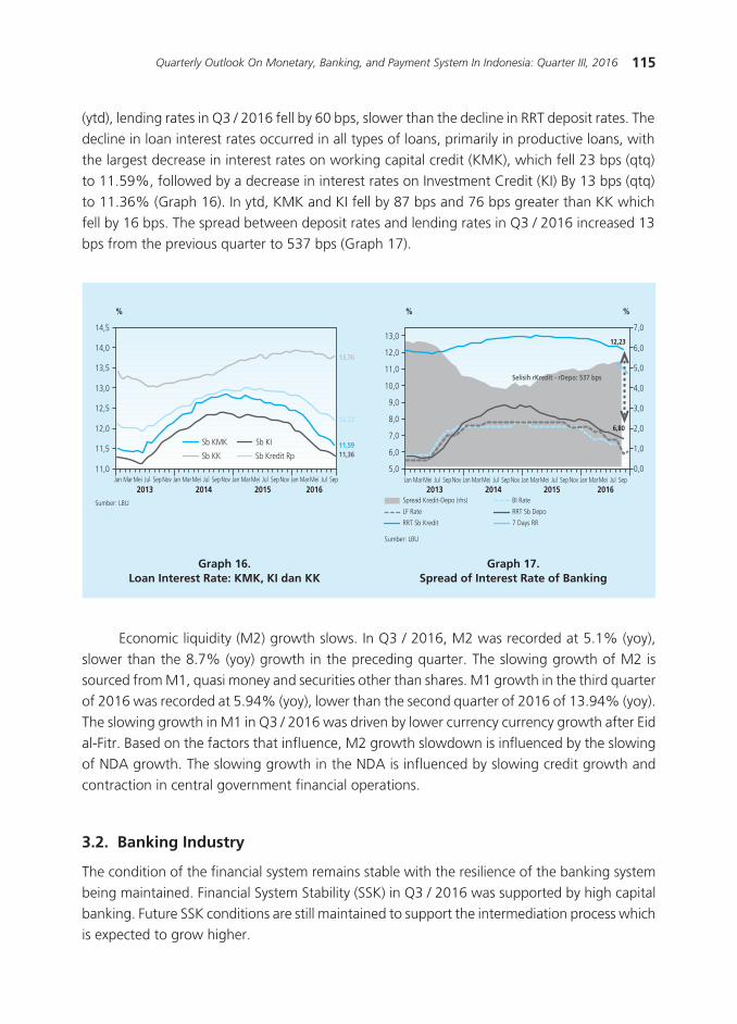
Transmission through credit lines has not been optimal, as evidenced by the limited loan growth in line with weak demand, including for investment needs from corporations. Credit growth was recorded at 6.5% (yoy), lower than the previous quarter’s growth of 7.9% (yoy). Lower credit growth in Q3 / 2016 was driven by lower growth in working capital credit (KMK) and investment credit (KI). Meanwhile, consumption credit (KK) growth remained relatively stable despite a slowing in Q3 / 2016 (Graph 18). By sector, credit growth in Q3 / 2016 in the majority of economic sectors was able to grow positively except for mining, industrial and freight sectors due to weak demand side in those sectors.
Third Party Funds Growth (DPK) in Q3 / 2016 slowed. DPK was recorded at 3.2% (yoy), slower than the previous quarter’s growth of 5.9% (yoy) (Graph 19). The slowing growth in DPK at the end of the third quarter of 2016, among others, occurred due to ransom payment by customers related to tax amnesty sourced from bank deposits. Based on its type, the slowing growth in DPK in Q3 / 2016 primarily came from the slowing growth in deposits and current accounts. The slowing growth in deposits is indicated by the income of the people as well as the transfer to other instruments. Meanwhile, the decrease in Giro growth is more related to fiscal behavior (NCG), especially the activity of transfer of funds to the account of the Regional Government. Meanwhile, savings growth is still in an increasing trend, increasing the ratio of Current Account, Saving Account (CASA) to 53.9%.
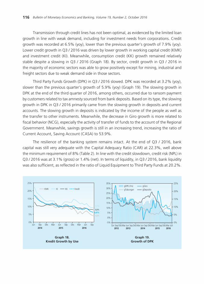
The resilience of the banking system remains intact. At the end of Q3 / 2016, bank capital was still very adequate with the Capital Adequacy Ratio (CAR) at 22.3%, well above the minimum requirement of 8% (Table 2). In line with the credit slowdown, credit risk (NPL) in Q3 / 2016 was at 3.1% (gross) or 1.4% (net). In terms of liquidity, in Q3 / 2016, bank liquidity was also sufficient, as reflected in the ratio of Liquid Equipment to Third Party Funds at 20.2%.
Graph 18.Kredit Growth by Use
Graph 19.Growth of DPK
��� ��� ��� ��� ��� ��� ��� ��� ��� ������� ���� ����
��
��
���
���
���
���
���� ��������
����
���������
����
���
���
���
���
���
���
��
��
������ ��� ��� ��� ��� ������ ��� ��� ������ ��� ��� ������ ������
���� ���� ���� ���� ����
���
���
���
��
��
���
��� ���� �� ������ ���������
117Quarterly Outlook On Monetary, Banking, and Payment System In Indonesia: Quarter III, 2016
3.3. Stock Market and State Securities Market
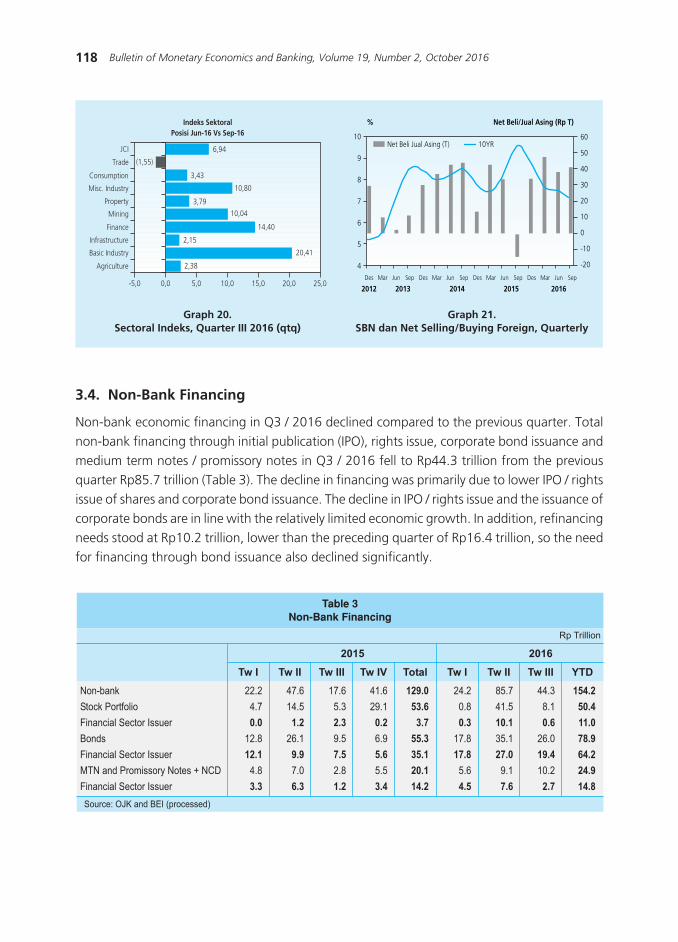
The development of the domestic stock market during Q3 / 2016 showed an increase, driven in part by various domestic and global positive factors. On September 30, 2016, the JCI reached 5,364.8 points or rose 348 points (6.94%, qtq) (Graph 20). On the domestic side, the JCI was boosted by better-than-expected quarterly economic data releases in Q3 / 2016, including a surplus in trade balance, second quarter economic growth in 2016 that was higher than in the previous quarter, rising foreign exchange reserves and relatively stable inflation. In addition, the tax amnesty program also encourages positive sentiment in the stock market. Meanwhile, from the global side, rising stock market performance was generally influenced by expectations of a declining FFR rise following the release of unreliable US economic data.
In line with the stock market, the SBN market showed a positive performance. Improved SBN market conditions are characterized by declining yield on government securities across all tenors. Overall yield fell 48 bps to 6.98% in Q3 / 2016 from 7.46% in Q2 2016. Short, medium and long term yields decreased by 56 bps, 46 bps and 44 bps to 6.56%, 7.01% and 7.45% respectively. Meanwhile, the benchmark 10-year tenor yield fell by 39 bps to 7.06% from 7.45%. The improvement is driven by global and domestic positive factors, which are relatively similar to the positive factors driving the improvement of the JCI. Amid declining yield on government securities, nonresident investors posted a net buy of Rp40.8 trillion in Q3 / 2016, up from the preceding quarter of Rp37.9 trillion (Graph 21).
����
�������������������
����������������������������������
����
���������
������������ ��� �� �� � ��� ��� ��� �� ���
�����������
� ������� ��������
����
���������������������������
� ������������ ������������������
���������������������������
�� �������������� �����
�������������������
������
������
������
���
���
���
���
���
��������
��������
��������
�����
����
�����
����
����
��������
��������
��������
�����
����
�����
����
����
��������
��������
��������
�����
����
�����
����
����
��������
��������
��������
�����
����
�����
����
����
��������
��������
��������
�����
����
�����
����
����
��������
��������
��������
�����
����
�����
����
����
��������
��������
��������
�����
����
�����
����
����
��������
��������
��������
�����
����
�����
����
����
��������
��������
��������
�����
����
�����
����
����
�����
��������
��������
�����
����
�����
����
����
118 Bulletin of Monetary Economics and Banking, Volume 19, Number 2, October 2016
Graph 20.Sectoral Indeks, Quarter III 2016 (qtq)
Graph 21.SBN dan Net Selling/Buying Foreign, Quarterly
3.4. Non-Bank Financing
Non-bank economic financing in Q3 / 2016 declined compared to the previous quarter. Total non-bank financing through initial publication (IPO), rights issue, corporate bond issuance and medium term notes / promissory notes in Q3 / 2016 fell to Rp44.3 trillion from the previous quarter Rp85.7 trillion (Table 3). The decline in financing was primarily due to lower IPO / rights issue of shares and corporate bond issuance. The decline in IPO / rights issue and the issuance of corporate bonds are in line with the relatively limited economic growth. In addition, refinancing needs stood at Rp10.2 trillion, lower than the preceding quarter of Rp16.4 trillion, so the need for financing through bond issuance also declined significantly.
���
�����
�����������
���� ���������
�������
�����
�������
��������������
��������������
����������
����
����
�����
���������
�����
��
����
���
����
��� ��� �� ���� ��� ��� ��
�������������������������� �������� �
�������������������������
����
��������������������� ���������
����
����
�����
�����������
���������
����������
�����������������
������������������
������������
����������������
������
������������
����������������������
��������
�����������
�����������������������������
�������������� ������������������������������������������������������������������ ��������������������������������������������
����� ������ ����� ��� � ���� ����� ������ ��
� ���������
Net Beli/Jual Asing (Rp T)
2012 2013 2014 2015 2016Des Mar Jun Sep Des Mar Jun Sep Des Mar Jun Sep Des Mar Jun Sep
%
10
9
8
7
6
5
4
60
50
40
30
20
10
0
-10
-20
10YRNet Beli Jual Asing (T)
119Quarterly Outlook On Monetary, Banking, and Payment System In Indonesia: Quarter III, 2016
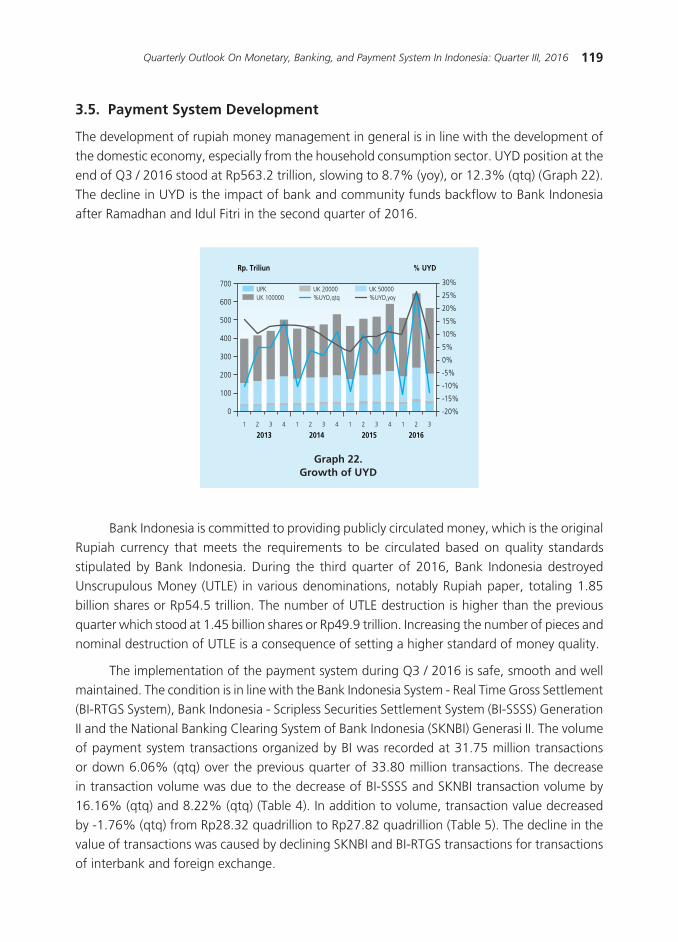
Graph 22.Growth of UYD
3.5. Payment System Development
The development of rupiah money management in general is in line with the development of the domestic economy, especially from the household consumption sector. UYD position at the end of Q3 / 2016 stood at Rp563.2 trillion, slowing to 8.7% (yoy), or 12.3% (qtq) (Graph 22). The decline in UYD is the impact of bank and community funds backflow to Bank Indonesia after Ramadhan and Idul Fitri in the second quarter of 2016.
Rp. Triliun % UYD
2013 2014 2015 2016
30%
25%
20%
15%
10%
5%
0%
-5%
-10%
-15%
-20%
1 2 3 4 1 2 3 4 1 2 3 4 1 2 3
700
600
500
400
300
200
100
0
UPKUK 100000
UK 20000 UK 50000%UYD,qtq %UYD,yoy
Bank Indonesia is committed to providing publicly circulated money, which is the original Rupiah currency that meets the requirements to be circulated based on quality standards stipulated by Bank Indonesia. During the third quarter of 2016, Bank Indonesia destroyed Unscrupulous Money (UTLE) in various denominations, notably Rupiah paper, totaling 1.85 billion shares or Rp54.5 trillion. The number of UTLE destruction is higher than the previous quarter which stood at 1.45 billion shares or Rp49.9 trillion. Increasing the number of pieces and nominal destruction of UTLE is a consequence of setting a higher standard of money quality.
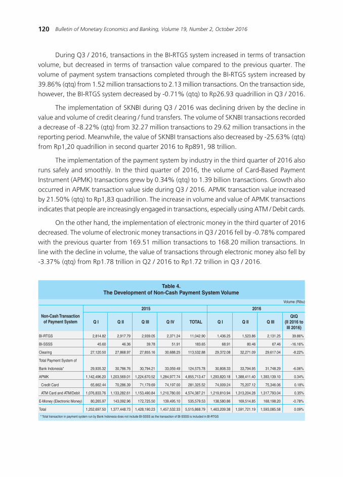
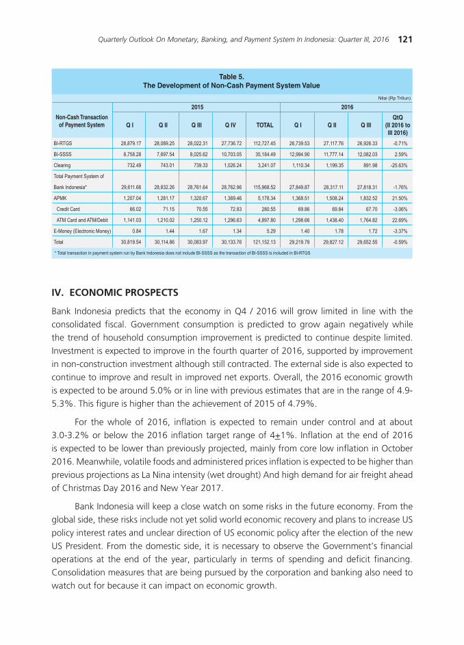
The implementation of the payment system during Q3 / 2016 is safe, smooth and well maintained. The condition is in line with the Bank Indonesia System - Real Time Gross Settlement (BI-RTGS System), Bank Indonesia - Scripless Securities Settlement System (BI-SSSS) Generation II and the National Banking Clearing System of Bank Indonesia (SKNBI) Generasi II. The volume of payment system transactions organized by BI was recorded at 31.75 million transactions or down 6.06% (qtq) over the previous quarter of 33.80 million transactions. The decrease in transaction volume was due to the decrease of BI-SSSS and SKNBI transaction volume by 16.16% (qtq) and 8.22% (qtq) (Table 4). In addition to volume, transaction value decreased by -1.76% (qtq) from Rp28.32 quadrillion to Rp27.82 quadrillion (Table 5). The decline in the value of transactions was caused by declining SKNBI and BI-RTGS transactions for transactions of interbank and foreign exchange.
120 Bulletin of Monetary Economics and Banking, Volume 19, Number 2, October 2016
During Q3 / 2016, transactions in the BI-RTGS system increased in terms of transaction volume, but decreased in terms of transaction value compared to the previous quarter. The volume of payment system transactions completed through the BI-RTGS system increased by 39.86% (qtq) from 1.52 million transactions to 2.13 million transactions. On the transaction side, however, the BI-RTGS system decreased by -0.71% (qtq) to Rp26.93 quadrillion in Q3 / 2016.
The implementation of SKNBI during Q3 / 2016 was declining driven by the decline in value and volume of credit clearing / fund transfers. The volume of SKNBI transactions recorded a decrease of -8.22% (qtq) from 32.27 million transactions to 29.62 million transactions in the reporting period. Meanwhile, the value of SKNBI transactions also decreased by -25.63% (qtq) from Rp1,20 quadrillion in second quarter 2016 to Rp891, 98 trillion.
The implementation of the payment system by industry in the third quarter of 2016 also runs safely and smoothly. In the third quarter of 2016, the volume of Card-Based Payment Instrument (APMK) transactions grew by 0.34% (qtq) to 1.39 billion transactions. Growth also occurred in APMK transaction value side during Q3 / 2016. APMK transaction value increased by 21.50% (qtq) to Rp1,83 quadrillion. The increase in volume and value of APMK transactions indicates that people are increasingly engaged in transactions, especially using ATM / Debit cards.
On the other hand, the implementation of electronic money in the third quarter of 2016 decreased. The volume of electronic money transactions in Q3 / 2016 fell by -0.78% compared with the previous quarter from 169.51 million transactions to 168.20 million transactions. In line with the decline in volume, the value of transactions through electronic money also fell by -3.37% (qtq) from Rp1.78 trillion in Q2 / 2016 to Rp1.72 trillion in Q3 / 2016.
Q I Q II Q III Q IV TOTAL Q I Q II Q IIIQtQ
(II 2016 toIII 2016)
BI-RTGS 2,814.82 2,917.79 2,939.05 2,371.24 11,042.90 1,436.25 1,523.86 2,131.25 39.86%
BI-SSSS 45.60 46.36 39.78 51.91 183.65 68.91 80.46 67.46 -16.16%
Clearing 27,120.50 27,868.97 27,855.16 30,688.25 113,532.88 29,372.08 32,271.09 29,617.04 -8.22%
Total Payment System of
Bank Indonesia* 29,935.32 30,786.76 30,794.21 33,059.49 124,575.78 30,808.33 33,794.95 31,748.29 -6.06%
APMK 1,142,496.20 1,203,569.01 1,224,670.52 1,284,977.74 4,855,713.47 1,293,820.18 1,388,411.40 1,393,139.10 0.34%
Credit Card 65,662.44 70,286.39 71,179.69 74,197.00 281,325.52 74,009.24 75,207.12 75,346.06 0.18%
ATM Card and ATM/Debit 1,076,833.76 1,133,282.61 1,153,490.84 1,210,780.00 4,574,387.21 1,219,810.94 1,313,204.28 1,317,793.04 0.35%
E-Money (Electronic Money) 80,265.97 143,092.96 172,725.50 139,495.10 535,579.53 138,580.86 169,514.85 168,198.20 -0.78%
Total 1,252,697.50 1,377,448.73 1,428,190.23 1,457,532.33 5,515,868.79 1,463,209.38 1,591,721.19 1,593,085.58 0.09%
* Total transaction in payment system run by Bank Indonesia does not include BI-SSSS as the transaction of BI-SSSS is included in BI-RTGS
Non-Cash Transactionof Payment System
2015 2016
Table 4.The Development of Non-Cash Payment System Volume
Volume (Ribu)
121Quarterly Outlook On Monetary, Banking, and Payment System In Indonesia: Quarter III, 2016
IV. ECONOMIC PROSPECTS
Bank Indonesia predicts that the economy in Q4 / 2016 will grow limited in line with the consolidated fiscal. Government consumption is predicted to grow again negatively while the trend of household consumption improvement is predicted to continue despite limited. Investment is expected to improve in the fourth quarter of 2016, supported by improvement in non-construction investment although still contracted. The external side is also expected to continue to improve and result in improved net exports. Overall, the 2016 economic growth is expected to be around 5.0% or in line with previous estimates that are in the range of 4.9- 5.3%. This figure is higher than the achievement of 2015 of 4.79%.
For the whole of 2016, inflation is expected to remain under control and at about 3.0-3.2% or below the 2016 inflation target range of 4+1%. Inflation at the end of 2016 is expected to be lower than previously projected, mainly from core low inflation in October 2016. Meanwhile, volatile foods and administered prices inflation is expected to be higher than previous projections as La Nina intensity (wet drought) And high demand for air freight ahead of Christmas Day 2016 and New Year 2017.
Bank Indonesia will keep a close watch on some risks in the future economy. From the global side, these risks include not yet solid world economic recovery and plans to increase US policy interest rates and unclear direction of US economic policy after the election of the new US President. From the domestic side, it is necessary to observe the Government’s financial operations at the end of the year, particularly in terms of spending and deficit financing. Consolidation measures that are being pursued by the corporation and banking also need to watch out for because it can impact on economic growth.
Q I Q II Q III Q IV TOTAL Q I Q II Q IIIQtQ
(II 2016 toIII 2016)
* Total transaction in payment system run by Bank Indonesia does not include BI-SSSS as the transaction of BI-SSSS is included in BI-RTGS
Non-Cash Transactionof Payment System
2015 2016
Table 5.The Development of Non-Cash Payment System Value
Nilai (Rp Triliun)
BI-RTGS
BI-SSSS
Clearing
Total Payment System of
Bank Indonesia*
APMK
Credit Card
ATM Card and ATM/Debit
E-Money (Electronic Money)
Total
28,879.17
8,758.28
732.49
29,611.66
1,207.04
66.02
1,141.03
0.84
30,819.54
28,089.25
7,697.54
743.01
28,832.26
1,281.17
71.15
1,210.02
1.44
30,114.86
28,022.31
8,025.62
739.33
28,761.64
1,320.67
70.55
1,250.12
1.67
30,083.97
27,736.72
10,703.05
1,026.24
28,762.96
1,369.46
72.83
1,296.63
1.34
30,133.76
112,727.45
35,184.49
3,241.07
115,968.52
5,178.34
280.55
4,897.80
5.29
121,152.13
26,739.53
12,994.90
1,110.34
27,849.87
1,368.51
69.86
1,298.66
1.40
29,219.79
27,117.76
11,777.14
1,199.35
28,317.11
1,508.24
69.84
1,438.40
1.78
29,827.12
26,926.33
12,082.03
891.98
27,818.31
1,832.52
67.70
1,764.82
1.72
29,652.55
-0.71%
2.59%
-25.63%
-1.76%
21.50%
-3.06%
22.69%
-3.37%
-0.59%

122 Bulletin of Monetary Economics and Banking, Volume 19, Number 2, October 2016
This page intentionally left blank
123Early Warning System and Currency Volatility Management In Emerging Market
EARLY WARNING SYSTEM AND CURRENCY VOLATILITY MANAGEMENT IN EMERGING MARKET
Natasia Engeline S1
Salomo Posmauli Matondang2
This paper adopts theoretical models from Candelon, Dumitrescu, and Hurlin and empirical model
from Commerzbank to devise a set of indicators that can serve as an early warning system (EWS) on
exchange rate. In light of the appreciation of emerging countries’ currencies during the Fed quantitative
easing period, it is important to understand on how The Fed normalization would put pressure on managing
volatility for central banks, especially for countries with large trade and fiscal deficit such as Indonesia.
All in all, using both EWS models, central banks could discern potential exchange rate depreciation for
intervention purpose.
Abstract
Keywords: Dynamic Logit Model, Foreign Exchange, Early Warning System, Emerging Countries,
Foreign Exchange Intervention
JEL Classification: C32, E58, F31, F37
1 Financial Analyst, Reserve Management Department of Bank Indonesia ([email protected])2 Financial Analyst, Reserve Management Department of Bank Indonesia ([email protected])
124 Bulletin of Monetary Economics and Banking, Volume 19, Number 2, October 2016
I. INTRODUCTION
Research on emerging countries’ exchange rate dynamics has been the subject of interest by academia, market participants, and financial regulators; considering their high volatility. Central banks especially those in emerging market economies are taking special interest in exchange rate dynamics due to their role in stabilizing exchange rate movement through intervention. Gracia et al. (2011) argued that the role of central bank intervention in exchange rate movement is desirable, especially in vulnerable emerging economies. Alder and Tovar (2011), Basu and Varoudakis (2013), and Neely (2008), identified several motives of the central bank’s intervention such as moderate exchange rate volatility, reducing exchange rate misalignment, accumulate reserves, and supply foreign exchange to the market.
More recently, following the unconventional policies of major advanced economies from 2008, emerging countries’ currencies have experienced appreciation due to massive capital inflow. Looking forward, it is important to understand on how The Federal Reserve normalization would put pressure for central banks on managing volatility, especially those with large trade and fiscal deficit such as Indonesia. In retrospect, initial reports that The Federal Reserve might begin “tapering” its quantitative easing on May 2013, caused a rush to exit from emerging countries including Indonesia, with exchange rate declines of as much as 20% in the following four months.
Considering the importance of intervention in managing emerging currencies, central banks in emerging market economies should devise a set of indicators that can serve as an early warning system (EWS); which could identify an impending depreciation before it occurs. EWS could help central banks implement optimal policies including the strategies of intervention to prevent or smooth the impact of currency depreciation.
Kaminsky, Lizondo, and Reinhart (1998) pioneered a comprehensive survey regarding EWS by proposing several case studies of devaluation episodes using structural model of balance of payment crises, signaling model for currency crises, as well as empirical study using macroeconomic and financial data for emerging countries. Berg and Patillo (1999) proposed a static panel probit model as an alternative to the signaling approach. Bussiere and Fratzcher (2006) proposed a multinominal logit EWS that consider the crisis as a ternary variable instead of binary.
Unfortunately, in previous studies, EWS have remained silent at the recent financial crisis. The difficulty to detect potential currency depreciation lies in the specificity of EWS that aimed at accurately detecting the occurrence of a currency depreciation which is translated into a binary variable that takes the value of one when depreciation occurs and the value of zero otherwise. In this context, it is not possible to directly implement the method proposed in times series econometrics such as vector autoregression. Furthermore, most previous EWS are static and assume that the depreciation probability depends only on a set of macroeconomic variables.
125Early Warning System and Currency Volatility Management In Emerging Market
3 Detail explanation on constrained maximum likelihood is available on appendix.
Candelon, Dumitrescu, and Hurlin (2010) proposed a new generation of EWS which reconcile the limited dependent property of the depreciation variable and the dynamic dimension of this phenomenon. In particular, Candelon et al. (2010) considered not only the exogenous source of depreciation persistence from macroeconomic data, but also endogenous persistence of depreciation which are lagged binary depreciation variable and past index associated to the probability of being in depreciation period. Thus, the EWS relies an autoregressive (AR) model, where the endogenous variable summarizes all the past information of the system. Given all these different specifications, an exact maximum likelihood estimation by Kauppi and Saikonnen (2008) is used to estimate the models.3
In contrast from academic EWS model, Commerzbank (2013) proposed a simple currency depreciation index that requires a shorter forecast period and does not require regular recalibration. Commerzbank used several macroeconomics indicators such as current account and industrial production as well as market indicators such as real effective exchange rate and equity market performance that translated into risk measures with equal weighting.
Perhaps the most interesting feature of our research is on how we adopt both models from Candelon et al. (2010) and Commerzbank (2013) to give a better understanding toward potential currency depreciation. All in all, using both EWS model, central banks could discern potential exchange rate depreciation for intervention purpose.
This paper is structured as follows. Section 2 describes the structure of early warning signal (EWS) by Candelon et al. (2010) and Commerzbank as well as several assumptions for the EWS index. Section 3 describes the data and construction of the EWS index. Section 4 reports the forecast evaluation and intervention strategies, while section 5 concludes.
II. THEORY
The first model is a dynamic EWS based on Candelon et al. (2010) that exploits the persistence property of the currency depreciation captured by lagged endogenous indicators. The second model is based on Commerzbank that use macroeconomics and market indicators to construct a depreciation warning index.
2.1. Dating Currency Depreciation
Before elaborating further into the EWS model, we define currency depreciation as large market movement adjusted for interest rate differentials rather that looking at composite indices of exchange rate pressure as elaborated by Kumar et al. (2002). Thus, if et is the exchange rate vis-à-vis the US dollar and rt and rt
* are domestic and foreign (US) interest rates of maturity D,
we supposed that depreciation takes place if
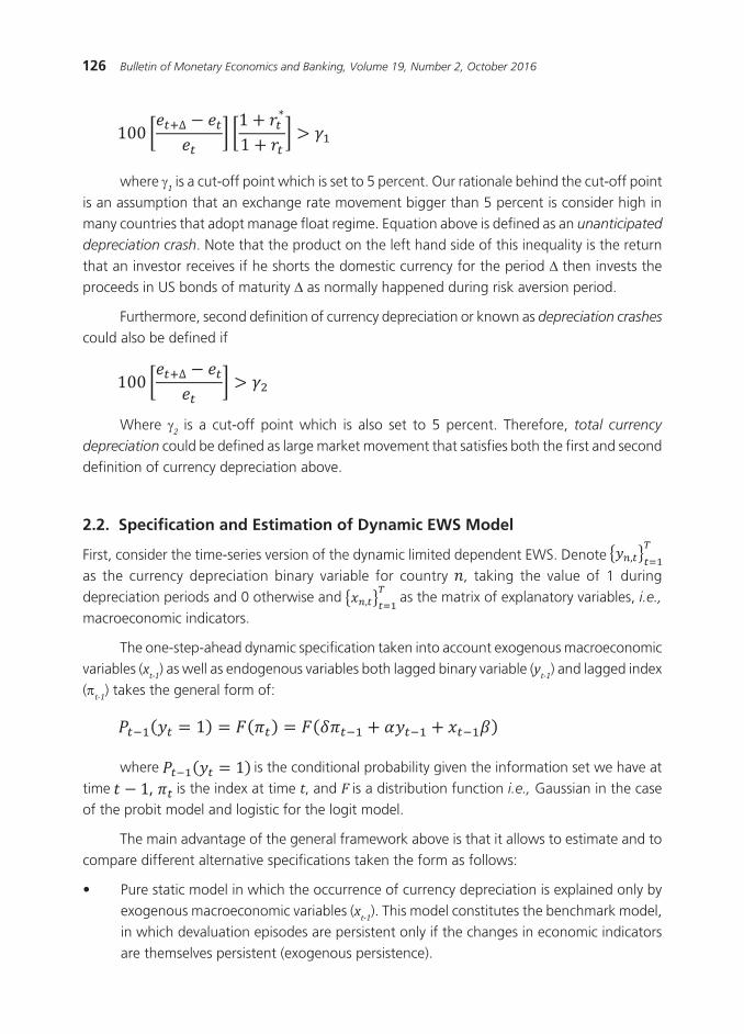
126 Bulletin of Monetary Economics and Banking, Volume 19, Number 2, October 2016
where g1 is a cut-off point which is set to 5 percent. Our rationale behind the cut-off point is an assumption that an exchange rate movement bigger than 5 percent is consider high in many countries that adopt manage float regime. Equation above is defined as an unanticipated
depreciation crash. Note that the product on the left hand side of this inequality is the return that an investor receives if he shorts the domestic currency for the period D then invests the proceeds in US bonds of maturity D as normally happened during risk aversion period.
Furthermore, second definition of currency depreciation or known as depreciation crashes could also be defined if
Where g2 is a cut-off point which is also set to 5 percent. Therefore, total currency
depreciation could be defined as large market movement that satisfies both the first and second definition of currency depreciation above.
2.2. Specification and Estimation of Dynamic EWS Model
First, consider the time-series version of the dynamic limited dependent EWS. Denote as the currency depreciation binary variable for country , taking the value of 1 during depreciation periods and 0 otherwise and as the matrix of explanatory variables, i.e., macroeconomic indicators.
The one-step-ahead dynamic specification taken into account exogenous macroeconomic variables (xt-1) as well as endogenous variables both lagged binary variable (yt-1) and lagged index (pt-1) takes the general form of:
where is the conditional probability given the information set we have at time is the index at time t, and F is a distribution function i.e., Gaussian in the case of the probit model and logistic for the logit model.
The main advantage of the general framework above is that it allows to estimate and to compare different alternative specifications taken the form as follows:
• Purestaticmodelinwhichtheoccurrenceofcurrencydepreciationisexplainedonlybyexogenous macroeconomic variables (xt-1). This model constitutes the benchmark model, in which devaluation episodes are persistent only if the changes in economic indicators are themselves persistent (exogenous persistence).
127Early Warning System and Currency Volatility Management In Emerging Market
• Dynamicmodelinwhichtheoccurrenceofcurrencydepreciationisexplainedbyexogenousmacroeconomic variables and lagged value of the binary dependent variable (yt-1). In this case, probability of currency depreciation is affected by the regime prevailing in the previous period on the depreciation probability.
• Dynamicmodelinwhichtheoccurrenceofcurrencydepreciationisexplainedbyexogenousmacroeconomic variables and lagged index (pt-1). In this case, probability of currency depreciation increases linearly with the rise of index.
• Finally,themostcomplexdynamicmodel,includingboththelaggeddependentvariable(yt-1) and the lagged index (pt-1). In this case, probability of currency depreciation is affected by the regime prevailing in the previous period and increases linearly with the rise of index.
Furthermore, since the last two models have d as an autoregressive parameter, it has to satisfy the usual stationarity condition. Otherwise, the depreciation becomes perpetual, which is counterintuitive. In order to overcome this problem, a constrained maximum likelihood estimation is implemented which general form of the log-likelihood function could be described as follows
where q is the vector parameters. Given the maximum-likelihood framework, dynamic time-series models are easy to implement.
2.3. Specification and Estimation of Commerzbank Model
Commerzbank (2013) developed a simple and intuitive EWS model, using both macroeconomic indicator and market indicator, that requires shorter forecast period, does not require regular recalibration, and makes clear contribution of individual inputs to the overall risk signal.
128 Bulletin of Monetary Economics and Banking, Volume 19, Number 2, October 2016
Macroeconomics indicators that are being used to construct the index are as follows
• Currentaccount: This gives an indication of the degree to which a country relies on foreign funding. Higher current account surplus may translate into lower volatility in the currency.
• Moneysupply: Excessive money creation may lead to higher inflation and consequently a weaker currency.
• Inflation: Excessive inflation will typically lead to depreciation of the currency.
• Industrial production: Falling industrial production may signal that the economy is weakening. Lower interest rate and/or a weaker currency may be required to stimulate a recovery thus triggering currency depreciation.
• Tradedata (exports): A sharp fall in exports will lessen demand for the currency. A weaker currency may in any case be necessary to increase the competitiveness of the export market.
• Shorttermdebt: High level of short term debt increases the risk of a funding crisis should debt become difficult to roll over.
• Non-performingloans: An elevated ratio of non-performing loans could lead to weaker economic growth if not a banking crisis.
• Domesticcredit: Very high level or credit to the domestic private sector may indicate excesses in the banking system.
• Economicsurprises: Worse than expected economic data may result from deterioration in the economy that could lead to the withdrawal of capital from local assets and consequent weakening of the currency.
Market indicators that are being used to construct the index are as follows
• Realeffectiveexchangerate: The trade-weighted average exchange rate, adjusted for differing price levels in home and foreign markets, provides a gauge of a country’s external competitiveness. If a country’s REER increases too strongly, it may signal that the currency needs to depreciate.
• FXimpliedvolatility: The level of FX implied volatility acts as a proxy for option prices and hence the approximate cost of hedging. An increased level of hedging activity may be indicative of concern over a weakening of the currency.
• Equitymarketperformance: Weaker asset markets can lead to withdrawal of foreign capital. If investors repatriate the realized funds there will be selling pressure on the local currency.
129Early Warning System and Currency Volatility Management In Emerging Market
• Globalrisksentiment: The global risk environment can influence currency markets through the home bias effect – investors in developed markets are more likely to withdraw funds from emerging markets when risk is perceived as being high.
Commerzbank model use simple steps to generate a warning index as follows :
• Rankeachdatapointwithrespecttoitsownhistory.
• Convertpercentilerankings intoriskmeasures.Wherea lowervalueismorelikelytocause for concern, i.e., industrial production, the risk level is given by one hundred minus the percentile ranking, otherwise the risk measure is simply given by the rank.
• Risk rankings for allmacroeconomic andmarket indicators for an individual countryare simply averaged to generate an overall risk rating on a scale from 0 to 100 for the currency in question.
• Riskindexiscalculatedusingequalweighting
2.4. Optimal Cut-Off
In order to compare the depreciation probabilities obtained from EWS model with the actual currency depreciation, we have to shift these probabilities to depreciation forecasts by defying an optimal threshold or cut-off that determine between potential currency depreciation and calm periods. If the probability of a depreciation is greater than the cut-off, the model issues a signal of a forthcoming depreciation. The lower the threshold is, the more signals the model will send, but at the same time, the number of wrong signals rises. On the other hand, higher threshold level reduces the number of wrong signals, but increases the number of missing signals. Thus, an indicator variable of predicting potential depreciation in currency for could be defined as follows, where C represents a fixed cut-off:
We address this trade-off by using the sensitivity and specificity methods to define an optimal cut-off of an index. For given value of the cut-off C, where , there are four conditions which are true positive, false positive, true negative, and false negative, as describe in the following matrix:
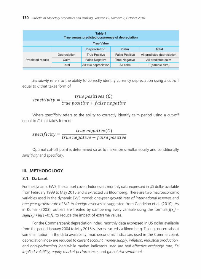
130 Bulletin of Monetary Economics and Banking, Volume 19, Number 2, October 2016
������������
������������
����
�����
������������� ���
�� ����������
������������
������ ��������������
��������������
�� ��������
��������
��������������������������
������������������
���������������
����������������������������������������� �������������
���� �����
����������
Sensitivity refers to the ability to correctly identify currency depreciation using a cut-off equal to C that takes form of
Where specificity refers to the ability to correctly identify calm period using a cut-off equal to C that takes form of
Optimal cut-off point is determined so as to maximize simultaneously and conditionally sensitivity and specificity.
III. METHODOLOGY
3.1. Dataset
For the dynamic EWS, the dataset covers Indonesia’s monthly data expressed in US dollar available from February 1999 to May 2015 and is extracted via Bloomberg. There are two macroeconomic variables used in the dynamic EWS model: one-yeargrowthrateofinternationalreserves and one-yeargrowthrateofM2toforeignreserves as suggested from Candelon et al. (2010). As in Kumar (2003), outliers are treated by dampening every variable using the formula f(xt) = sign(xt) * ln(1+|xt|), to reduce the impact of extreme values.
For the Commerzbank depreciation index, monthly data expressed in US dollar available from the period January 2004 to May 2015 is also extracted via Bloomberg. Taking concern about some limitation in the data availability, macroeconomic indicators used in the Commerzbank depreciation index are reduced to current account, money supply, inflation, industrial production, and non-performing loan while market indicators used are realeffectiveexchangerate,FXimplied volatility, equity market performance, and global risk sentiment.
131Early Warning System and Currency Volatility Management In Emerging Market
3.2. Model Evaluation and Robustness Test
In order to show the usefulness of the model, we implement the EWS evaluation by Candelon et al. (2011), especially to test their forecasting abilities (out-of-sample exercises). The main advantage of this framework is that it can be applied to any EWS outputting depreciation probabilities, both in-sample and out-of-sample. To be more precise, first, we rely on different evaluation criteria and comparison tests to identify the outperforming model. Second, we gauge the optimal model’s ability to discriminate between depreciation and calm periods by identifying the optimal cut-off for each model.
Accordingly, we consider both classic EWS evaluation measures such as the QPS criterion and newer one for the EWS literature, which take the cut-off into account in the evaluation and thus lead to a more refined diagnostic, i.e. the AreaUndertheROCcriterion(AUC). The QPS criterion is a mean-squared-error measure that compares the depreciation probabilities (the forecasts issued by the EWS, Pt-1 (yt = 1)) with the depreciation occurrence indicator yt:
At the same time, AUC is a credit-scoring criteria, that reveals the predictive abilities of an EWS by relying on all the values of the gut-off, i.e. the threshold used to compute depreciation forecasts :
Where represents the sensitivity, i.e. the proportion of depreciation correctly identified by the EWS for a given cut-off c and is the specificity, i.e. the proportion of calm periods correctly identified by the model for a cut-off equal to c.
Next, the optimal cut-offis identified by maximizing the Youden index ( ) which is an accuracy measure arbitrating between type I and type II errors (misidentified depreciation and false alarms):
where . A model’s ability to correctly discriminate between depreciation and calm periods is the given by sensitivity and specificity. For more details on the evaluation method, see Candelon et al. (2011).

132 Bulletin of Monetary Economics and Banking, Volume 19, Number 2, October 2016
IV. RESULT AND ANALYSIS
4.1. Estimation Results for Dynamic EWS
General form of dynamic EWS elaborated above has main advantage that it allows to estimate and compare different EWS specification. First, we estimate the three types of dynamic EWS as well as the benchmark which is the static EWS model under analysis in the time-series framework. Furthermore, the static model is labeled as Model 1, a dynamic one which includes the lagged binary dependent variable is labeled as Model 2, a dynamic one including the lagged index is labeled as Model 3, and finally, a dynamic model which includes both the lagged binary dependent variable and the lagged index is labeled as Model 4.
Second, we find the best goodness of fit from the four models by relying on Schwarz Information Criterion (SBC). SBC reveals that the right-hand-side variables have important explanatory power. Based on the lowest values of the SCB criterion, Model 2 that includes the lagged binary dependent variable seems to be the most adequate model to predict potential currency depreciation. Thus, SCB gives a clear indication that dynamic model generally outperform the static one.
Third, we analyze the signs of the estimated parameters for the Model 2. The result shows a negative coefficient of growth of international reserves, indicating a decline in the probability of currency depreciation is presumed with an increase in a country’s growth of international
reserves. Intuitively, an increase in growth of international reserves indicates currency non-vulnerability. For the growthofM2toreservescoefficient, it is assumed that if the growth of the amount of money in circulation overruns the growth of international reserves, the currency is perceived as unstable and a speculative attack is foreseeable. Thus, a positive coefficient of the growthofM2reserves is expected. Nonetheless, a negative coefficient that appears on growthofM2toreservesmight be due to the fact that the two macroeconomic variables capture mainly the information not filtered by the lagged binary variable. Most importantly, the coefficient of the lagged binary dependent variable is significant and has a positive sign. It means that the probability of being in a deprecation episode increases if a depreciation period prevailed in the previous period. This clearly indicates that depreciation’ persistence should be accounted for in order to improve accuracy of currency EWS.
��������� ������ ������ ������ ������
��������������������������������� �����������������������
������� ������� ������� ������� �������
��� ��� ��� ���
�� ������������ ���� � ��������� ��������������������� ��������������������������������� ��� �� ������ ��������������� ������
133Early Warning System and Currency Volatility Management In Emerging Market
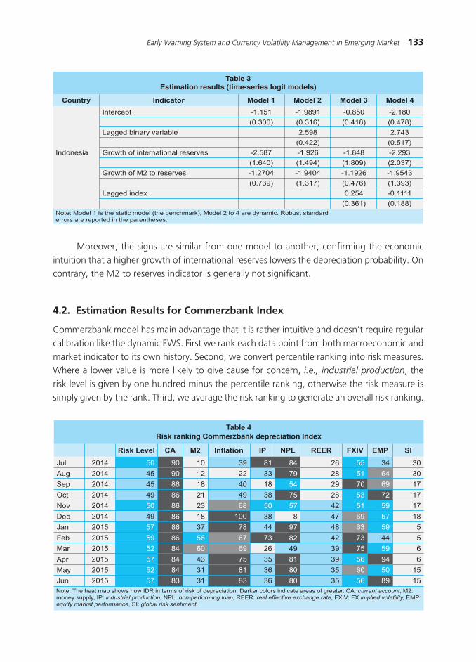
Moreover, the signs are similar from one model to another, confirming the economic intuition that a higher growth of international reserves lowers the depreciation probability. On contrary, the M2 to reserves indicator is generally not significant.
4.2. Estimation Results for Commerzbank Index
Commerzbank model has main advantage that it is rather intuitive and doesn’t require regular calibration like the dynamic EWS. First we rank each data point from both macroeconomic and market indicator to its own history. Second, we convert percentile ranking into risk measures. Where a lower value is more likely to give cause for concern, i.e., industrial production, the risk level is given by one hundred minus the percentile ranking, otherwise the risk measure is simply given by the rank. Third, we average the risk ranking to generate an overall risk ranking.
�������
���������
����������������������������������������� ����������
���������
�������������������� �
�������������������� ���������
����������������������
������������
�������������
���������� �������� ������
������������������� ����������� ���� � �������
��������� ���
���� ���������������� ������� �������
��������� ������ ������������������������ ���������������������
��������� ������� ������� ������ �������
���������� �������������������� �������������������� ������ ������������������������������������������������������������������
����������
�������������������������������� ������������ ��
���
���
������
���
���
���
�� ���
�����
�������������������������������������������������������������������������������������������������������������������������������� ������������ ������������������������� ������������������������ ������������������ ��������������� ����������������� �������� ��������������������������� ��������������������������
���������
���
���
������
���
������
���
���
�� �� ������� � �� ��� �� ��� �� ��
����
��
��
����
�
��
�
����
������
��
��
����
��
����
��
��
�����
�
�
����
��
����
��
��
��
��
��
�����
��
����
��
����
������
��
��
����
��
���
��
��
������
��
��
���
�
����
��
��
���
�
�
����
�
����
��
��
������
��
��
����
��
����
��
��
����
��
��
����
��
���
��
���
������
�
��
����
��
����
��
��
134 Bulletin of Monetary Economics and Banking, Volume 19, Number 2, October 2016
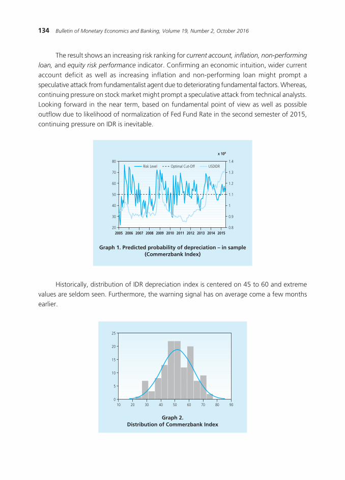
The result shows an increasing risk ranking for currentaccount,inflation,non-performingloan, and equity risk performance indicator. Confirming an economic intuition, wider current account deficit as well as increasing inflation and non-performing loan might prompt a speculative attack from fundamentalist agent due to deteriorating fundamental factors. Whereas, continuing pressure on stock market might prompt a speculative attack from technical analysts. Looking forward in the near term, based on fundamental point of view as well as possible outflow due to likelihood of normalization of Fed Fund Rate in the second semester of 2015, continuing pressure on IDR is inevitable.
Graph 1. Predicted probability of depreciation – in sample (Commerzbank Index)
��
��
��
��
��
��
������ ���� ���� ���� ���� ���� ���� ���� ���� ���� ����
���
���
���
���
�
���
���
�����
������� �� ������������ ������
Historically, distribution of IDR depreciation index is centered on 45 to 60 and extreme values are seldom seen. Furthermore, the warning signal has on average come a few months earlier.
Graph 2.Distribution of Commerzbank Index
��
��
��
��
�
��� �� �� �� �� �� �� �� ��
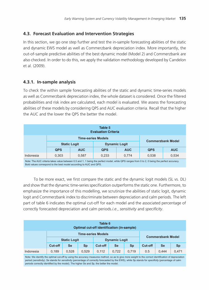
135Early Warning System and Currency Volatility Management In Emerging Market
4.3. Forecast Evaluation and Intervention Strategies
In this section, we go one step further and test the in-sample forecasting abilities of the static and dynamic EWS model as well as Commerzbank depreciation index. More importantly, the out-of-sample predictive abilities of the best dynamic model (Model 2) and Commerzbank are also checked. In order to do this, we apply the validation methodology developed by Candelon et al. (2009).
4.3.1. In-sample analysis
To check the within sample forecasting abilities of the static and dynamic time-series models as well as Commerzbank depreciation index, the whole dataset is considered. Once the filtered probabilities and risk index are calculated, each model is evaluated. We assess the forecasting abilities of these models by considering QPS and AUC evaluation criteria. Recall that the higher the AUC and the lower the QPS the better the model.
���
��������� ����� ����� ����� ����� ����� �����
��������������������������
��� ��� ��� ��� ���
������������ �������������
�����������������������������
���� ������������������������������������������������������������� �������������������������� ������������������������� ����������������������������������������������������������������������������
To be more exact, we first compare the static and the dynamic logit models (SL vs. DL) and show that the dynamic time-series specification outperforms the static one. Furthermore, to emphasize the importance of this modelling, we scrutinize the abilities of static logit, dynamic logit and Commerzbank index to discriminate between depreciation and calm periods. The left part of table 6 indicates the optimal cut-off for each model and the associated percentage of correctly forecasted depreciation and calm periods.i.e., sensitivity and specificity.
�������
��������� ����� ����� ����� ����� ����� ����� ��� ����� �����
�������������������������� ��������� ��� �������
������������ �������������
��� �� �� ��� ������ �������� �
��������������������������������������������������������������������������������������������������������������������������������� ���������������������������������� ������������������������������������������������������������������ ����������������������������������������������������������������������������������������
� �� ������� � �� ������� � ��
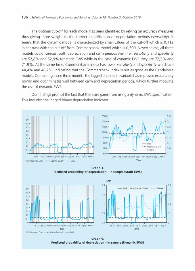
136 Bulletin of Monetary Economics and Banking, Volume 19, Number 2, October 2016
The optimal cut-off for each model has been identified by relying on accuracy measures thus giving more weight to the correct identification of depreciation periods (sensitivity). It seems that the dynamic model is characterized by small values of the cut-off which is 0,112 in contrast with the cut-off from Commerzbank model which is 0,500. Nevertheless, all three models could forecast both depreciation and calm periods well. i.e., sensitivity and specificity are 52,8% and 52,9% for static EWS while in the case of dynamic EWS they are 72,2% and 71,9%. At the same time, Commerzbank index has lower sensitivity and specificity which are 44,4% and 46,2%, indicating that the Commerzbank index is not as good as the Candelon’s models. Comparing those three models, the lagged dependent variable has improved explanatory power and discriminates well between calm and depreciation periods, which further motivate the use of dynamic EWS.
Our findings prompt the fact that there are gains from using a dynamic EWS specification. This includes the lagged binary depreciation indicator.
Graph 3.Predicted probability of depreciation – in sample (Static EWS)
Graph 4.Predicted probability of depreciation – in sample (Dynamic EWS)
�
���
���
���
���
���
���
���
���
���
�
������ ������ ����� ������ ������ ����� ������ ������ �����
����������� ��������������� � �
������ ������ ������������ ������ ������ ������ ������ ����������
����
����
����
�����
�����
�����
�����
�
� ��
� �
� ��
� �
� ��
� �
� ��
���������������������
����
���������� ������ ������ ������ ������ ������ ������ ������ ������
�
���
���
���
���
��
���
���
���
���
�
����������� ��������������� � �
�����
���������� ������ ������ ������ ������ ������ ������ ������ ������
���
���
�
���
���
�
���
���
���
������ ��������������� �����
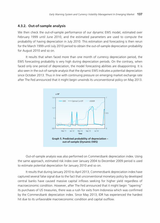
137Early Warning System and Currency Volatility Management In Emerging Market
4.3.2. Out-of-sample analysis
We then check the out-of-sample performance of our dynamic EWS model, estimated over February 1999 until June 2010, and the estimated parameters are used to compute the probability of having depreciation in July 2010. This estimation and forecasting is then rerun for the March 1999 until July 2010 period to obtain the out-of-sample depreciation probability for August 2010 and so on.
It results that when faced more than one month of currency depreciation period, the EWS forecasting probability is very high during depreciation periods. On the contrary, when faced only one period of depreciation, the model forecasting abilities are disappointing. It is also seen in the out-of-sample analysis that the dynamic EWS indicates a potential depreciation since October 2013. Thus in line with continuing pressure on emerging market exchange rate after The Fed announced that it might begin unwinds its unconventional policy on May 2013.
Graph 5. Predicted probability of depreciation –out-of-sample (Dynamic EWS)
�����
���������� ������ ������ ������ ������
��
�
���
���
�
�
�� ��������������� ������
Out-of-sample analysis was also performed on Commerzbank depreciation index. Using the same approach, estimated risk index over January 2004 to December 2009 period is used to estimate potential depreciation for January 2010 and so on.
It results that during January 2010 to April 2013, Commerzbank depreciation index have captured several false signal due to the fact that unconventional monetary policy by developed central banks have caused massive capital inflows seeking for higher yield regardless of macroeconomic condition. However, after The Fed announced that it might begin “tapering” its purchases of US treasuries, there was a rush for exits from Indonesia which was confirmed by the Commerzbank depreciation index. Since May 2013, IDR has experienced the hardest hit due to its unfavorable macroeconomic condition and capital outflow.
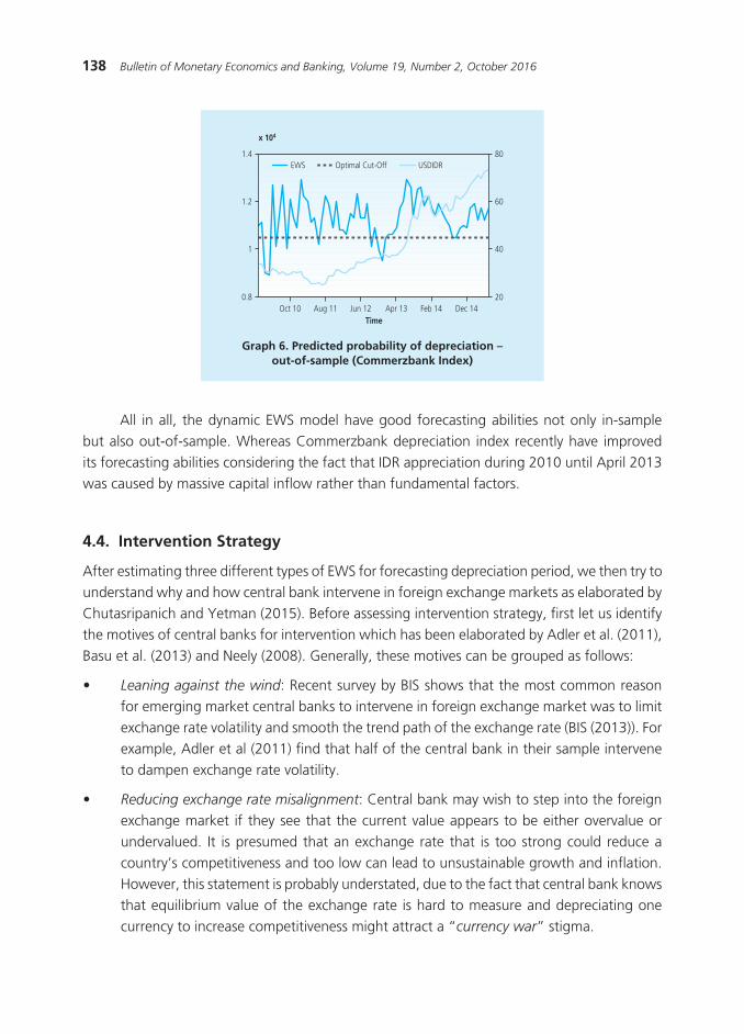
138 Bulletin of Monetary Economics and Banking, Volume 19, Number 2, October 2016
All in all, the dynamic EWS model have good forecasting abilities not only in-sample but also out-of-sample. Whereas Commerzbank depreciation index recently have improved its forecasting abilities considering the fact that IDR appreciation during 2010 until April 2013 was caused by massive capital inflow rather than fundamental factors.
4.4. Intervention Strategy
After estimating three different types of EWS for forecasting depreciation period, we then try to understand why and how central bank intervene in foreign exchange markets as elaborated by Chutasripanich and Yetman (2015). Before assessing intervention strategy, first let us identify the motives of central banks for intervention which has been elaborated by Adler et al. (2011), Basu et al. (2013) and Neely (2008). Generally, these motives can be grouped as follows:
• Leaningagainstthewind: Recent survey by BIS shows that the most common reason for emerging market central banks to intervene in foreign exchange market was to limit exchange rate volatility and smooth the trend path of the exchange rate (BIS (2013)). For example, Adler et al (2011) find that half of the central bank in their sample intervene to dampen exchange rate volatility.
• Reducingexchangeratemisalignment: Central bank may wish to step into the foreign exchange market if they see that the current value appears to be either overvalue or undervalued. It is presumed that an exchange rate that is too strong could reduce a country’s competitiveness and too low can lead to unsustainable growth and inflation. However, this statement is probably understated, due to the fact that central bank knows that equilibrium value of the exchange rate is hard to measure and depreciating one currency to increase competitiveness might attract a “currency war” stigma.
Graph 6. Predicted probability of depreciation –out-of-sample (Commerzbank Index)
�����
����
���
�
���
���
��
��
��
��
������ ������ ������ ����� ����� �����
��� ��������������� ����
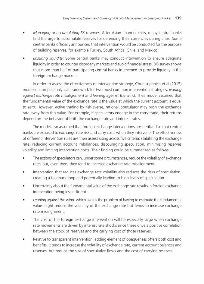
139Early Warning System and Currency Volatility Management In Emerging Market
• ManagingoraccumulatingFXreserves: After Asian financial crisis, many central banks find the urge to accumulate reserves for defending their currencies during crisis. Some central banks officially announced that intervention would be conducted for the purpose of building reserves, for example Turkey, South Africa, Chile, and Mexico.
• Ensuring liquidity: Some central banks may conduct intervention to ensure adequate liquidity in order to counter disorderly markets and avoid financial stress. BIS survey shows that more than half of participating central banks intervened to provide liquidity in the foreign exchange market.
In order to assess the effectiveness of intervention strategy, Chutasripanich et al (2015) modeled a simple analytical framework for two most common intervention strategies: leaning
against exchange rate misalignment and leaning against the wind. Their model assumed that the fundamental value of the exchange rate is the value at which the current account is equal to zero. However, active trading by risk-averse, rational, speculator may push the exchange rate away from this value. For example, if speculators engage in the carry trade, their returns depend on the behavior of both the exchange rate and interest rates.
The model also assumed that foreign exchange interventions are sterilized so that central banks are exposed to exchange rate risk and carry costs when they intervene. The effectiveness of different intervention rules are then assess using across five criteria: stabilizing the exchange rate, reducing current account imbalances, discouraging speculation, minimizing reserves volatility and limiting intervention costs. Their finding could be summarized as follows:
• Theactionsofspeculatorscan,undersomecircumstances,reducethevolatilityofexchangerates but, even then, they tend to increase exchange rate misalignment.
• Interventionthatreducesexchangeratevolatilityalsoreducestherisksofspeculation,creating a feedback loop and potentially leading to high levels of speculation.
• Uncertaintyaboutthefundamentalvalueoftheexchangerateresultsinforeignexchangeintervention being less efficient.
• Leaningagainstthewind,which avoids the problem of having to estimate the fundamental value might reduce the volatility of the exchange rate but tends to increase exchange rate misalignment.
• Thecostoftheforeignexchangeinterventionwillbeespeciallylargewhenexchangerate movements are driven by interest rate shocks since these drive a positive correlation between the stock of reserves and the carrying cost of those reserves.
• Relativetotransparentintervention,addingelementofopaquenessoffersbothcostandbenefits. It tends to increase the volatility of exchange rate, current account balances and reserves, but reduce the size of speculative flows and the cost of carrying reserves.
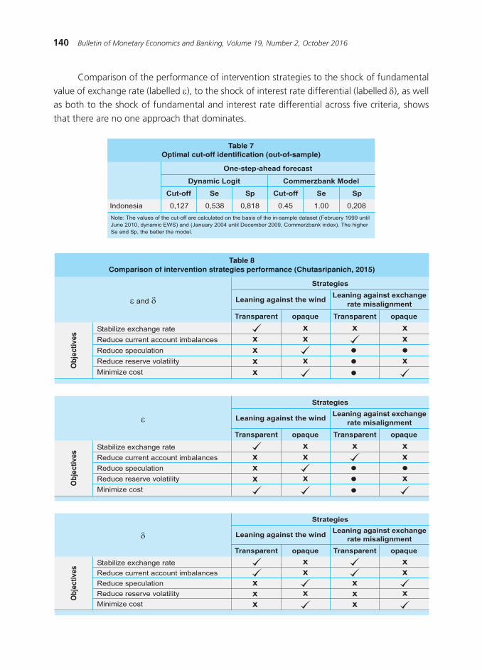
140 Bulletin of Monetary Economics and Banking, Volume 19, Number 2, October 2016
Comparison of the performance of intervention strategies to the shock of fundamental value of exchange rate (labelled ε), to the shock of interest rate differential (labelled d), as well as both to the shock of fundamental and interest rate differential across five criteria, shows that there are no one approach that dominates.
�������
��������� ����� ����� ����� ���� ���� �����
�������������������������� ��������� ���������������
������������� ������ ��������
����������������������
������������������������������������������������������������������������������ ������������������������������������������������������ �����������������������������������������������������
�� �� ������� �� ��
����������������������������������������� ����������������������������� ��������������� ������������������ ��
���������������������������������������� �����������������������������������
����������
������������������������������������������������
�����������������
���������� ���� ���������� ����
���
�����
��
�������
����
��
�
� ��
�
�����������������������
������������������ ��������������
��������������� �
�������������� ������������������ ��
����������
������������������������������������������������
�����������������
���������� ���� ���������� ����
���
�����
��
�
���
��
�
� ��
�
�����������������������
������������������ ��������������
��������������� �
�������������� ��������
���������� ��
����������
������������������������������������������������
�����������������
���������� ���� ���������� ����
���
�����
��
�
��
��
�
��
��
���
141Early Warning System and Currency Volatility Management In Emerging Market
V. CONCLUSION
Considering the importance of intervention in managing emerging currencies, this paper provides two EWS models that could be used to discern potential exchange rate depreciation for intervention purpose. In addition, this paper also outline several intervention strategies and their effectiveness in order to prepare for The Fed normalization that would put pressure on managing volatility for central banks, especially those with large trade and fiscal deficit such as Indonesia.
Several conclusions can be drawn from using both the dynamic EWS and Commerzbank index as well as incorporating them into intervention strategies. First, we show that in the in-sample test, dynamic logit models (sensitivity and specificity 72,2% and 71,9%) outperform static one (sensitivity and specificity 52,8% and 52,9%) as well as Commerzbank depreciation index (sensitivity and specificity 44,4% and 46,2%). Second, by combining both EWS, we could have a better predictive ability of potential currency depreciation. Since the dynamic EWS give better predictive ability both within in-sample an out-sample analysis, it is easier to assume that dynamic EWS alone would deliver adequate signals to discern potential currency depreciation. However, Commerzbank depreciation index could give us a better understanding of individual risk ranking for both macroeconomics and market indicators. Third, assessing the intervention strategy to lean against the wind to the shock of fundamental value of exchange rate (considering deteriorating fundamental condition in Indonesia) as well as to the shock of interest rate differential (normalization of Fed Fund Rate), it is suggested that some degree of opaqueness might help to limit speculation and minimize cost. However, if the main objective is to stabilize exchange rate, leaning against the wind transparently might be optimal. Furthermore, it is also suggested that cost of the foreign exchange intervention will be especially large when exchange rate movements are driven by interest rate shocks (Fed normalization)
Looking ahead, continuing pressures on IDR is inevitable. Nonetheless, there is no doubt that using both EWS model, central bank could implement optimal policies including the strategies of intervention to prevent or smooth the impact of currency depreciation.
142 Bulletin of Monetary Economics and Banking, Volume 19, Number 2, October 2016
REFERENCES
Adler, G., and Tovar, C.E., (2011). Foreign Exchange Intervention: A Shield Against Appreciation Winds?, IMF Working Paper 11/165.
Bank for International Settlements, (2005). Foreign Exchange Market Intervention in Emerging Markets: Motives, Techniques and Implication, BIS Papers 24.
Bank for International Settlements, (2013). Market Volatility and Foreign Exchange Intervention in EMEs: What has Changed?, BIS Papers 73.
Basu, K., and Varoudakis, A., (2013). How to Move the Exchange Rate if You Must: The Diverse Practice of Foreign Exchange Intervention by Central Banks and a Proposal for Doing it Better, World Bank Policy Research Working Paper 6460.
Berg, A., and Pattillo, C., (1999). Predicting Currency Crises: The Indicators Approach and an Alternative, Journal of International Money and Finance, 18, 561-586.
Bussiere, M., and Fratzscher, M., (2006). Towards a New Early System of Financial Crises, Journal of International Money and Finance, 25(6), 953-973.
Candelon, B., Dumitrecu, E.I., Hurlin, C., (2009). How to evaluate an Early Warning System? Towards a Unified Statistical Framework for Assessing Financial Crises Forecasting Methods, Working Paper.
Candelon, B., Dumitrecu, E.I., Hurlin, C., (2010). Currency Crises Early Warning System: why they should be Dynamic, Working Paper.
Commerzbank, (2013). Emerging Market Currency Exposure: How to Hedge and Manage Exposures to High Yield, Volatile Currencies, Commerzbank.
Falcetti, E., Tudela, M., (2006). Modelling Currency Crises in Emerging Markets: A Dynamic Probit Model with Unobserved Heterogeneity and Autocorrelated Errors, Oxford Bulletin of Economics and Statistics, 68(4), pages 445-471.
Frankel, J.A., Yetman, J., (1990). Chartists, Fundamentalist and Trading in The Foreign Exchange Market, American Economic Review, 80(2), pages 181-185.
Fuertes, A.M., Kalotychou, E., (2007). Optimal Design of Early Warning Systems for Sovereign Debt Crises, International Journal of Forecasting, 23(1), 85-100
Gallant, A.R., (1987). Nonlinear Statistical Models, John Wiley and Sons, New York.
Gracia, C.J., Restrepo, J.E., and Roger, S., (2011). How Much Should Inflation Targeters Care About the Exchange Rate?, Journal of International Money and Finance 30(7), 1590-1617.
143Early Warning System and Currency Volatility Management In Emerging Market
Harding, D., and Pagan A., (2009). An Econometric Analysis of Some Models for Constructed Binary Time Series, NCER Working Paper 39.
Kaminsky, G., Lizondo, S., Reinhart, C., (1998). Leading Indicators of Currency Crises, IMF Staff papers, 45 (1), 1-48.
Kauppi, H., Saikkonen, P., (2008), Predicting U.S. Recession with Dynamic Binary Response Models, The Review of Economics and Statistics, 90 (4), 777-791.
Kumar, M., Moorthy, U., and Perraudin, W., (2003) Predicting Emerging Market Currency Crashes, Journal of Empirical Finance, 10, 427-454.
Neely, C.J., (2001), The Practice of Central Bank Intervention: Looking Under the Hood, Federal Reserve Bank of St. Louis Review May/June, 1-10.
Neely, C.J., (2001), Central Bank Authorities’ Believe about Foreign Exchange Intervention, Journal of International money and Finance, 27(1), pages 1-25.
144 Bulletin of Monetary Economics and Banking, Volume 19, Number 2, October 2016
Recall the general form of the model in the case of a logistic distribution function. Following Kauppi and Saikkonen, the
initial value p0 is set to , being the sample mean of exogenous variables. The initial condition for the β vector of parameters is given by an OLS estimation, while the initial d is set to 0. Moreover, since d is an autoregressive parameter, a constrained maximum likelihood estimation must be implemented. Nevertheless, the same results can be reached in a faster and easier way, by using a transformation of the d parameter in the classical maximum likelihood process. Thus, to solve this problem, denote the new maximization parameter by ψ, identified so that d is equal to , i.e., d takes value in the interval [0,1].
Hence, the log-likelihood function takes the form of:
AppENDIx: CONSTRAINED MAxIMUM LIKELIhOOD ESTIMATION (KAUppI AND SAIKKKONEN, 2008)
where q is the vector of parameters q = [ , a, β].
It is noticed that in view of the parameter transformation from d to ψ, the maximization variance-covariance matrix corresponds to the parameters [ψ,a,β], and not to the initial parameters [d,a,β]. Thus, we must proceed to a change of the variance-covariance matrix from the first space to the second one. To this end, we use Taylor’s theorem to calculate the approximation of the transformation function around the point ψ0. To be more exact, since the estimated parameter , where , the approximation becomes:
Nevertheless, we aim at finding the variance of d, and thus, using the formula Var(a^’ X)=a^’ Var(X)a, we obtain:
Since , can be replace with the estimator
145Early Warning System and Currency Volatility Management In Emerging Market
Last but not least, the first derivative of the transformation function f( ) with respect to ( ) can be computed through finite differences. Consequently, the standard error obtained as the square root of the elements laying on the first diagonal of the variance-covariance matrix are consistent with the [ψ,a,β] vector of parameters. More exactly, a Gallant correction base on Parzen kernel (Gallant,1987) is used for the variance-covariance matrix. Kauppi et al. (2008) argue that robust standard errors can be obtained as the diagonal elements of the matrix , where
,
and where .
On top of that, consider that the robust variance-covariance matrix should be used not only for h-periods-afterhead forecasts, h>1 (as in Kauppi and Saikonnen, 2008) but also for one period-ahead forecasts, since the logistic distributional hypothesis imposed to the error term might not always hold and most importantly, since this variance-covariance matrix specification is robust to autocorrelation, automatically introduced when considering an EWS (Breg and Coke, 2004).

146 Bulletin of Monetary Economics and Banking, Volume 19, Number 2, October 2016
This page intentionally left blank
147The Impact of Geothermal Energy Sector Development on Electricity Sector In Indonesia Economy
THE IMPACT OF GEOTHERMAL ENERGY SECTOR DEVELOPMENT ON ELECTRICITY SECTOR
IN INDONESIA ECONOMY
Nayasari Aissa1 Djoni Hartono
Energy is one of the most important inputs that supports Indonesia’s economy. The government
utilises coal and oil as the main sources for power plants energy mix. However, the utilization of fossil fuel
energy has been proven to pose negative impacts on the environment such as, increasing carbon dioxide
emission which leads to global warming. This study analyses investment policy on increasing electricity
production of geothermal power plants as well as substitution of fossil energy to geothermal energy
using Computable General Equilibrium (CGE) Model and Indonesia’s data of Social Accounting Matrix
2008. The result shows that when investment on the substitution of energy from fossil to renewable
energy takes place, economic growth will increase and carbon dioxide emission will reduce significantly.
Abstract
Keywords: CGE, Electricity, CO2 Emission, Fossil Energy, Geothermal, Growth
JEL Classification: C68, O44, O21, Q4
1 Lecturer at Department of Economics–University of Indonesia ([email protected] and [email protected]).
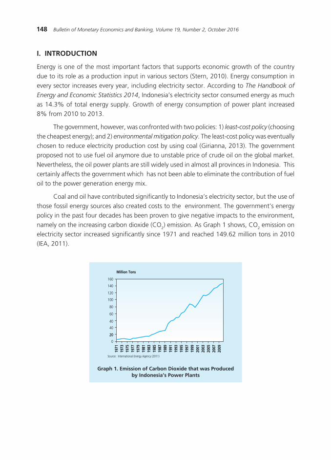
148 Bulletin of Monetary Economics and Banking, Volume 19, Number 2, October 2016
I. INTRODUCTION
Energy is one of the most important factors that supports economic growth of the country due to its role as a production input in various sectors (Stern, 2010). Energy consumption in every sector increases every year, including electricity sector. According to The Handbook of
Energy and Economic Statistics 2014, Indonesia’s electricity sector consumed energy as much as 14.3% of total energy supply. Growth of energy consumption of power plant increased 8% from 2010 to 2013.
The government, however, was confronted with two policies: 1) least-cost policy (choosing the cheapest energy); and 2) environmental mitigation policy. The least-cost policy was eventually chosen to reduce electricity production cost by using coal (Girianna, 2013). The government proposed not to use fuel oil anymore due to unstable price of crude oil on the global market. Nevertheless, the oil power plants are still widely used in almost all provinces in Indonesia. This certainly affects the government which has not been able to eliminate the contribution of fuel oil to the power generation energy mix.
Coal and oil have contributed significantly to Indonesia’s electricity sector, but the use of those fossil energy sources also created costs to the environment. The government’s energy policy in the past four decades has been proven to give negative impacts to the environment, namely on the increasing carbon dioxide (CO2) emission. As Graph 1 shows, CO2 emission on electricity sector increased significantly since 1971 and reached 149.62 million tons in 2010 (IEA, 2011).
Graph 1. Emission of Carbon Dioxide that was Producedby Indonesia’s Power Plants
Source: International Energy Agency (2011)
0
20
40
60
80
100
120
140
160
40
20
1971
1973
1975
1977
1979
1981
1983
1985
1987
1989
1991
1993
1995
1997
1999
2001
2003
2005
2007
2009
Million Tons
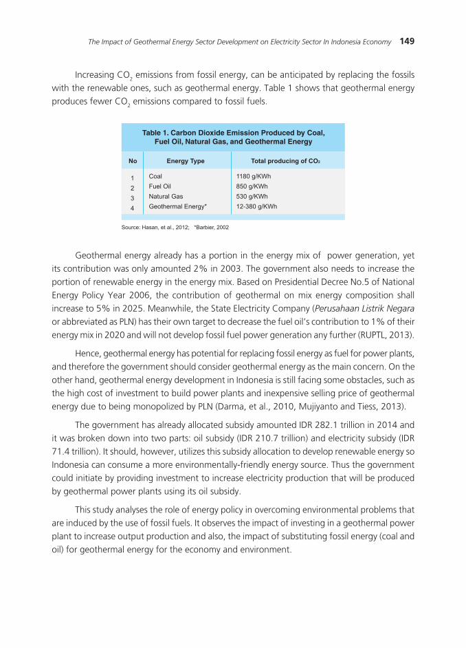
149The Impact of Geothermal Energy Sector Development on Electricity Sector In Indonesia Economy
Table 1. Carbon Dioxide Emission Produced by Coal,Fuel Oil, Natural Gas, and Geothermal Energy
No
1234
CoalFuel Oil Natural GasGeothermal Energy*
Source: Hasan, et al., 2012; *Barbier, 2002
1180 g/KWh850 g/KWh530 g/KWh12-380 g/KWh
Energy Type Total producing of CO2
Increasing CO2 emissions from fossil energy, can be anticipated by replacing the fossils with the renewable ones, such as geothermal energy. Table 1 shows that geothermal energy produces fewer CO2 emissions compared to fossil fuels.
Geothermal energy already has a portion in the energy mix of power generation, yet its contribution was only amounted 2% in 2003. The government also needs to increase the portion of renewable energy in the energy mix. Based on Presidential Decree No.5 of National Energy Policy Year 2006, the contribution of geothermal on mix energy composition shall increase to 5% in 2025. Meanwhile, the State Electricity Company (Perusahaan Listrik Negara or abbreviated as PLN) has their own target to decrease the fuel oil’s contribution to 1% of their energy mix in 2020 and will not develop fossil fuel power generation any further (RUPTL, 2013).
Hence, geothermal energy has potential for replacing fossil energy as fuel for power plants, and therefore the government should consider geothermal energy as the main concern. On the other hand, geothermal energy development in Indonesia is still facing some obstacles, such as the high cost of investment to build power plants and inexpensive selling price of geothermal energy due to being monopolized by PLN (Darma, et al., 2010, Mujiyanto and Tiess, 2013).
The government has already allocated subsidy amounted IDR 282.1 trillion in 2014 and it was broken down into two parts: oil subsidy (IDR 210.7 trillion) and electricity subsidy (IDR 71.4 trillion). It should, however, utilizes this subsidy allocation to develop renewable energy so Indonesia can consume a more environmentally-friendly energy source. Thus the government could initiate by providing investment to increase electricity production that will be produced by geothermal power plants using its oil subsidy.
This study analyses the role of energy policy in overcoming environmental problems that are induced by the use of fossil fuels. It observes the impact of investing in a geothermal power plant to increase output production and also, the impact of substituting fossil energy (coal and oil) for geothermal energy for the economy and environment.
150 Bulletin of Monetary Economics and Banking, Volume 19, Number 2, October 2016
II. THEORY
2.1. Theoretical Review
This research uses Computable General Equilibrium (CGE) model that is functioned for analysing impact of policy. CGE model uses general equilibrium basic theory that was first developed by Leon Walras in 1874. The general equilibrium theory explains the interaction of inter-market that reached equilibrium in economy simultaneously, given a change in the market, then it will affect other market in the economy.
This study analyses the impact of a whole economy when electricity sector is given more investment and fossil fuels are substituted for geothermal energy. According to Walras (1874), when there was a change on one sector,it would thus affect another sector and also affect the whole economy. The economic condition could reach equilibrium condition, if amount n -market in economy and amount n-1 -market have already reached their equilibrium condition.
2.1.1. Economic Growth and Energy
Stern (2010) modified the Solow Growth Theory (1) to observe the impact of economic growth when there was a substitution between energy and capital,
(1)
Y(t) represents output, K(t) represents capital, A(t) represents technology and L(t) represents labour, whereas A (t) L (t) represents effective labour.
The result shows that substituting capital to energy will increase employment opportunities and rising of income, thus it will affect to the increase of economic growth. The production function is,
(2)
Q is output (factory goods and services); X is input (capital and labour); E is several energy inputs (coal and fuel oil); and A shows indicator of total factor productivity (TFP).
2.1.2. Economic Growth and Investment in Infrastructure
According to Mankiw (2007), investment is divided into three types: a) business fixed investment (BFI), the elimination of goods and services that was done by the company, such as buying machine; (b) residential investment (RI), the investment that was done by household through buying property; and c) inventory investment (II), the changing on production factor, such as input that was used by company in the production process.
151The Impact of Geothermal Energy Sector Development on Electricity Sector In Indonesia Economy
An investment discussed in this study is the business fixed investment by investing in infrastructure, power generation for increasing output production. The main function of investing for investor is, to get recompensation of capital production factor.
Fedderke et al. (2008) argued that investment on infrastructure will give a positive impact on economic growth. The relationship between infrastructure and economic growth could be observed in two ways, directly or indirectly -related: 1) on directly related, infrastructure is observed as contributing sector to Gross Domestic Product (GDP) and as a production input to another sector, and 2) on indirectly related, when infrastructure was considered as complementary input on sector, thus it could increase productivity of other input factors.
2.2. Empirical Overview
There are numerous studies which explain the negative impact of the use of fossil energy on the environment. Aravena, et al. (2012) did a study on external cost that was caused by using fossil energy in a power plant. They suggested shifting to renewable energy to decrease carbon dioxide emission, and thus it would affect the external costs. Zou (2012) conducted a research to observe the negative impact of using fossil energy on power plant, thus there is a need to substitute fossil energy for hydroelectricity. Bravi and Basosi (2013), however, analysed that the used of renewable energy could in fact, increase CO2 emission.
Krozer (2011), Kose (2007) and Moreno et al (2012) used econometric methods to observe the impact of substituting fossil fuel energy for renewable energy on power plant, thus it could reduce electricity cost and make electricity cost cheaper for consumers. Ortega et al (2013) did approximation on cost and profit while using renewable energy for power plant.
Lu, et al. (2009) discussed the impact of investing in energy sector for increasing economic growth in one of provinces in China. Rose (1995) also analysed the positive impact on economic growth using the dynamic linear programming to get results from substituting fossil energy for renewable energy. Halkso and Tzeremes (2013) obtained a rather different result, though, that, utilization of renewable energy as input for power plant in the long term will only give positive impact for developed countries, and not for developing country. Ohler and Fetters (2014) also revealed that utilization geothermal energy to produce electricity will give small impact on GDP growth.
There are studies with CGE model which come up with different results. Aydin (2010), for instance, developed a dynamic CGE model for Turkey, called TurGEM-D, by simulating the increasing quantity of hydroelectricity to substitute the role of fossil energy that Turkey currently does not have. The result is that investment in renewable energy influences the rising of economic growth and reduces CO2 emission. Engida et al (2011) used static CGE model to show that investment in power plant gave positive results in economic growth. Dissou and Didic (2011) used recursive-dynamic CGE model to observe the impact of investing in infrastructure,
152 Bulletin of Monetary Economics and Banking, Volume 19, Number 2, October 2016
including power plant, that give positive effect on economic growth. Borojo (2012) obtained a specific result by using recursive-dynamic CGE model that investing in power plant using foreign direct investment s increases economic growth.
There are several studies that used CGE model for modelling energy policy: 1) the impact of the energy pricing policy on the increase of electricity consumer price (Isdinarmiarti, 2011); 2) the impact of energy policy to replace the use of fossil fuels with other energy (natural gas, coal, and other renewable energy) (Sugiyono, 2009); and 3) the impact of energy price changes in output of industrial sector (Nikensari (2001). However, the research on investment policy on the geothermal sector and its substitution with a static CGE model is something new for economics science in Indonesian context.
The author sees that the use of fossil energy has given a negative impact on the Indonesia’s air quality. Thus the government should begin to take action to start replacing fossil energy to renewable energy, namely geothermal energy, as an input source for the production of electricity generation.
III. METHODOLOGY AND DATA
3.1. Computable General Equilibrium Model
Computable General Equilibrium (CGE) Model uses basic foundation General Equilibrium Theory as mentioned above. This model is functioned to analyse interactions between consumers, producers, and market equilibrium conditions in the economy. A market equilibrium condition is a market-clearing condition that is occurred when consumers can consume all of the output produced by producers (Lewis, 1991).
The CGE model used is the standard model for Indonesia (see Appendix 1). Similar models can be seen on the Inter-Regional Model System of Analysis for Indonesia in 5 Regions (IRSA-INDONESIA 5). The model developed by Resosudarmo et al. (2009) for regional analysis. This CGE Model assumed Indonesia as an open economy whose was a price taker that did not contribute impact for global price.
Graph 2 shows the standard model of CGE related to the linkage across blocks on the model. The diagram flow is described the followings:
• CapitalandLandareaggregatedusingConstantElasticitySubstitutionfunctiontoformthe composite input;
• Compositeinputiscombinedwithintermediateinputs(energy&non-energy)toproducedomestic gross output, using the Leontief function;
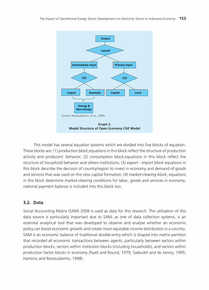
153The Impact of Geothermal Energy Sector Development on Electricity Sector In Indonesia Economy
This model has several equation systems which are divided into five blocks of equation. These blocks are: (1) production block,equations in this block reflect the structure of production activity and producers’ behavior; (2) consumption block,equations in this block reflect the structure of household behavior and others institutions; (3) export - import block equations in this block describe the decision of country/region to invest in economy and demand of goods and services that was used on the new capital formation; (4) market-clearing block, equations in this block determine market-clearing conditions for labor, goods and services in economy, national payment balance is included into this block too.
3.2. Data
Social Accounting Matrix (SAM) 2008 is used as data for this research. The utilisation of this data source is particularly important due to SAM, as one of data collection systems, is an essential analytical tool that was developed to observe and analyse whether an economic policy can boost economic growth and create more equitable income distribution in a country. SAM is an economic balance of traditional double-entry which is shaped into matrix partition that recorded all economic transactions between agents, particularly between sectors within production blocks, sectors within institution blocks (including households), and sectors within production factor blocks in economy (Pyatt and Round, 1979; Sadoulet and de Janvry, 1995; Hartono and Resosudarmo, 1998).
Graph 2.Model Structure of Open Economy CGE Model
Output
Leontif
CES
Intermediate input
Energy &Non-energy
CES
Primary Input
Import Domestic Capital Land
Source: Resosudarmo, et al., 2009
154 Bulletin of Monetary Economics and Banking, Volume 19, Number 2, October 2016
Furthermore, SAM is a useful data collection system due to: (1) SAM summarizes all of economic transaction that was occurred in economy system for a certain period. Thus, SAM could provide a general overview of economic system in the region; and (2) SAM describes social-economic structure. Thus, SAM is reliable to provide poverty and income distribution issue in economy (Hartono and Resosudarmo, 1998).
SAM is also an important analysis tools, because: (1) It could show substantial impact of economic policy towards household income. Thus, it could discover impact of economic policy towards poverty and income distribution issue. (2) It is relatively simple. Thus, the application could be easily done in various countries (Hartono and Resosudarmo, 1998).
In this study, we modified Indonesian SAM that is published by Central Agency on Statistics of Indonesia in 2008. There are two main differences between published Indonesian SAM and our modified Indonesian SAM: (i) It modifies ten household groups into two groups of households (decile groups of urban and rural households); (ii) It disaggregates sectors and commodities, hence generating more detailed sectors related to the energy, namely geothermal, natural gas, coal, gasoline, kerosene, high speed diesel oil (HSDO) and diesel oil. There are fourty four sector that are used in this study.
To conduct disaggregation of Indonesia SAM 2008 (published by BPS), this study used several information and supporting data, such as Input-Output tables and statistics of energy. The information about the structure of output and input follow the assumptions contained in those data.
IV. RESULT AND ANALYSIS
4.1. Empirical Review
Based on energy mix data of power plant in 2008, this research applies simulation scenarios. The main scenario is increasing the amount of investment for developing geothermal power generations and substituting a portion of fossil energy (coal and oil) for geothermal energy as an energy source for power plants, so that the electricity production will increase. There will be four scenarios which will be used for observing the impact of investing and substituting in geothermal sector for economic growth.
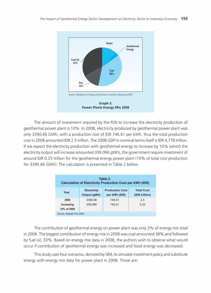
155The Impact of Geothermal Energy Sector Development on Electricity Sector In Indonesia Economy
Graph 3.Power Plants Energy Mix 2008
WaterGeothermalEnergy
Fuel Oil 33%
Gas 14%
Coal38%
Source: Handbook of Energy and Economics Statistics Indonesia (2009)
The amount of investment required by the PLN to increase the electricity production of geothermal power plant is 10%. In 2008, electricity produced by geothermal power plant was only 3390.66 GWh, with a production cost of IDR 746.61 per kWh, thus the total production cost in 2008 amounted IDR 2.5 trillion. The 2008 GDP in nominal terms itself is IDR 4,778 trillion. If we expect the electricity production with geothermal energy to increase by 10% (which the electricity output will increase amounted 339.066 gWh), the government require investment of around IDR 0.25 trillion for the geothermal energy power plant (10% of total cost production for 3390.66 GWh). The calculation is presented in Table 2 below.
Table 2. Calculation of Electricity Production Cost per kWh (IDR)
2008Increasing
10% of 2008
ElectricityOutput (gWh)
Production Costper kWh (IDR)
Total Cost(IDR trillion)
Year
3390.66339,066
746.61746.61
2.50.25
Source: Statistik PLN 2008
The contribution of geothermal energy on power plant was only 3% of energy mix total in 2008. The biggest contribution of energy mix in 2008 was coal amounted 38% and followed by fuel oil, 33%. Based on energy mix data in 2008, the authors wish to observe what would occur if contribution of geothermal energy was increased and fossil energy was decreased.
This study uses four scenarios, denoted by SIM, to simulate investment policy and substitute energy with energy mix data for power plant in 2008. Those are:
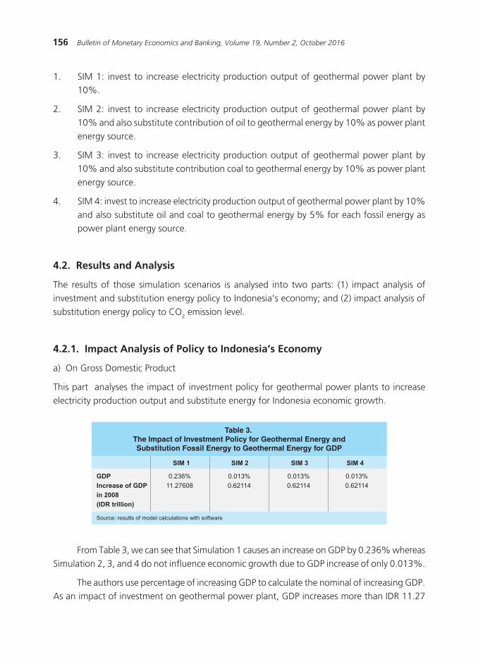
156 Bulletin of Monetary Economics and Banking, Volume 19, Number 2, October 2016
1. SIM 1: invest to increase electricity production output of geothermal power plant by 10%.
2. SIM 2: invest to increase electricity production output of geothermal power plant by 10% and also substitute contribution of oil to geothermal energy by 10% as power plant energy source.
3. SIM 3: invest to increase electricity production output of geothermal power plant by 10% and also substitute contribution coal to geothermal energy by 10% as power plant energy source.
4. SIM 4: invest to increase electricity production output of geothermal power plant by 10% and also substitute oil and coal to geothermal energy by 5% for each fossil energy as power plant energy source.
4.2. Results and Analysis
The results of those simulation scenarios is analysed into two parts: (1) impact analysis of investment and substitution energy policy to Indonesia’s economy; and (2) impact analysis of substitution energy policy to CO2 emission level.
4.2.1. Impact Analysis of Policy to Indonesia’s Economy
a) On Gross Domestic Product
This part analyses the impact of investment policy for geothermal power plants to increase electricity production output and substitute energy for Indonesia economic growth.
Table 3. The Impact of Investment Policy for Geothermal Energy andSubstitution Fossil Energy to Geothermal Energy for GDP
SIM 1 SIM 2 SIM 3 SIM 4
GDPIncrease of GDPin 2008(IDR trillion)
Source: results of model calculations with software
0.236%11.27608
0.013%0.62114
0.013%0.62114
0.013%0.62114
From Table 3, we can see that Simulation 1 causes an increase on GDP by 0.236% whereas Simulation 2, 3, and 4 do not influence economic growth due to GDP increase of only 0.013%.
The authors use percentage of increasing GDP to calculate the nominal of increasing GDP. As an impact of investment on geothermal power plant, GDP increases more than IDR 11.27

157The Impact of Geothermal Energy Sector Development on Electricity Sector In Indonesia Economy
trillion, meaning that investment in geothermal power plants amounted IDR 0.25 trillion will give profit as much as IDR 11.02 trillion for GDP in 2008. In the case of substitution of fossil energy for geothermal energy, nominal of GDP increases to IDR 0.37 trillion.
b) On Sectoral Output
SIM1 brings result that rail transport sector is the most affected by investment policy and substitution fossil energy to geothermal energy, the GDP increase is amounted 2.012%. The impacts are also happened in city-gas sector and non-subsidized energy sector with amount of increasing 1.894% and 0.781%, respectively. While, SIM 2, SIM 3, and SIM4 does not show significant impact for output sectoral, due to increasing portion geothermal energy in power plants energy mix of only 10%.
c) On Household Income
The household income that is mostly affected by increasing investment in a geothermal power plant, is the household within the category of urban-not poor, which increases by 0.528%. Meanwhile, the impacts on household income caused by substitution energy are felt by poor people in the village category, or increases by 0.020%. Poor households are defined as those with incomes below 20% (in decile 1 to decile 2), while the non-poor households is the rest.
4.2.2. Analysis Impact of Policy for Carbon Dioxide Emission
This part explains the impact of investment and substitution policy on power plants towards total of CO2 emission produced. Table 4 shows result of CO2 emission caused by energy substitution.
Substitution energy from coal to geothermal as an energy source for power plants by 10% affects decreasing of carbon dioxide emission by 5.92%. Whereas, energy substitution from oil to geothermal only decreases carbon dioxide emission by 1.56%. Substitution between a combination of coal and oil for geothermal energy as an energy source for power plants, though, decreases carbon dioxide emission by 3.74%.
SIM 2 SIM 3 SIM 4
Table 4. The Impact of Geothermal Energy Investment Policy andSubstitutions Fossil Energy for Geothermal Energy on
Reducing Carbon Dioxide Emission
Amount of Carbon DioxideEmission 2008
(million tons CO2)
102 -1.56% -5.92% -3.74%
The figure from SIM 3 indicates that replacing coal to geothermal energy will give significant impact for the decrease of CO2. It is due to the fact that coal is the biggest producer of CO2 when was used as the source of power plants in comparison with fuel oil.
158 Bulletin of Monetary Economics and Banking, Volume 19, Number 2, October 2016
V. CONCLUSIONS
This study aims to explain the electricity sector’s problems in Indonesia, especially environmental problem—increasing CO2 emission—that was produced by fossil energy power plants. Using a CGE model, we develop model to analyse the impact of policy towards economic condition and the amount of CO2 emission created, to support the development of geothermal energy as a source for power plants.
The simulation provides us several findings, first, the investment policy to increase geothermal power plant production increases GDP amounted IDR 11.02 trillion. The result is similar with Aydin (2010), Engida et al, (2011), Dissou and Didic (2011), and Borojo (2012) that investment in energy sector will give impact towards positive economic growth. Substitution from fossil energy to geothermal energy has insignificant effect, but still increases nominal of GDP amounted IDR 0.37 trillion.
Second finding from simulation is each sector increases when there is investment in geothermal power plants, the highest increase occurrs in transportation sector, which is the rail transport. Third, the household income affected the most by this investment policy is the household in urban-not poor category. Nonetheless, the substitution of fossil energy for geothermal energy does not affect significantly. Lastly, the substitutions energy from coal to geothermal energy affects more than that of oil to geothermal energy in the case of decreasing CO2 emission.
Investment and substitution policy to increase electricity production that is produced by geothermal energy has proven to give positive impact for economic growth and output sectoral. Substitution from fossil energy to geothermal energy is also confirmed to decrease total CO2 emission. This result could be the basis for the government to develop geothermal energy sector.
abcdefghijklmopqrstuvwxyzABCDEFGHIJKLMOPQRSTUVWXYZ
159The Impact of Geothermal Energy Sector Development on Electricity Sector In Indonesia Economy
abcdefghijklmopqrstuvwxyzABCDEFGHIJKLMOPQRSTUVWXYZ
REFERENCES
Aravena, C., et al. (2012). Environmental pricing of externalities from different sources of
electricity generation in Chile. Energy Economics 34, 1214-1225. Natural Resources, 1, 69-79.
Aydin, L. (2010). The Economic and Environmental Impacts of Constructing Hydro Power Plants
in Turkey: A Dynamic CGE Analysis (2004-2020). Natural Resources, 2010, 1, 69-79.
Barbier, E. (2002). Geothermal energy technology and current status: an overview. Renewable and Sustainable Energy Reviews 6, 3-65.
Borojo, D. G. (2012). The Economy Wide Impact of Investment on Infrastructure for Electricity
in Ethiopia: A Recursive Dynamic Computable General Equilibrium Approach. A Thesis Submitted to The School of Economics. Addis Ababa University.
Barron, J. M., et al. (2006). Understanding macroeconomic theory.Taylor&Francis.
Bravi,M.,&Basosi,R.(2014).Environmental impact of electricity from selected geothermal
power plants in Italy. Journal of Cleaner Production 66, 301-308.
Darma, S., et al. (2010). Geothermal Energy Update: Geothermal Energy Development and
Utilization in Indonesia. Proceedings World Geothermal Congress, Bali, Indonesia.
Dissou,Y.&Didic,S.(2011).Does Electricity Supply Strategy Matter? Shortage and Investment:
Reflections based on CGE Analysis. Research Project on the Distributive Impacts of Growth
Strategy. Department of Economics, University of Ottawa.
Engida, E. (2011). Does Electricity Supply Strategy Matter? Shortage and Investment: Reflections
based on CGE Analysis. EDRI Working Paper 006.
Fedderke,J.&Garlick,R.(2008).Infrastructure Development and Economic Growth in South
Africa: A Review of the Accumulated Evidence. Policy Paper Number 12.
Girianna, M., et al. (2013). New Development of Geothermal (Renewable) Energy in Indonesia. Indonesian Regional Science Association Conference 2013.
Halkos,G.&Tzeremes,N.(2013).The effect of electricity consumption from renewable sources
on countries’ economic growth levels: Evidence from advanced, emerging and developing
economies. MPRA Paper No. 50630, online at http://mpra.ub.uni-muenchen.de/50630/
Hartono,D.&Resosudarmo,B,P. (1998).Eksistensi Matriks Pengganda dan Dekkomposisi
Matriks Pengganda Pyatt dan Round dari Sistem Neraca Sosial Ekonomi. Ekonomi dan
Keuangan Indonesia. Vol XLVI, No. 4, hal 473-496.
160 Bulletin of Monetary Economics and Banking, Volume 19, Number 2, October 2016
Hasan, M. H., et al. (2012). A review on the pattern of electricity generation and emission in
Indonesia 1987 to 2009. Renewable and Sustaibale Energy Reviews 16, 3206 – 3219.
International Energy Agency. (2011). CO2 Emissions From Fuel Combustion Highlights 2011,
International Energy Agency of the OECD, Paris.
International Energy Agency. (2007). Energy Policy Review of Indonesia, IEA: Paris.
Isdinarmiati, T. (2011). Kenaikan Tarif Dasar Listrik dan Respon Kebijakan Untuk Meminimisasi
Dampak Negatif Terhadap Perekonomian. Tesis, Program Pascasarjana, Universitas Indonesia, Jakarta.
Kementrian Energi dan Sumber Daya Mineral. (2014). Handbook of Energy and Economics
Statistic of Indonesia.
Kementrian Energi dan Sumber Daya Mineral. (2009). Handbook of Energy and Economics
Statistic of Indonesia.
Kose, R. (2007). Geothermal Energy Potential for Power Generation in Turkey: A Case Study in
Simav, Kutahya. Renewable and Sustainable Energy Reviews 11, 497 -511.
Krozer, Y. (2011). Cost and Benefit of Renewable Energy in Europe. World Renewable Energy Congress, Swedia.
Lewis, J. D. (1991). A Computable General Equilibrium (CGE) Model of Indonesia. Development Discussion Paper No. 378. Harvard Institute for International Development, Harvard University.
Lu, C., et al. (2009). A CGE analysis to study the impacts on economic growth and carbon
dioxide emissions: A case of Shaanxi Province in western China. Energy 35, 4319-4327.
Mankiw, N. G. (2007). Brief Principles of Macroeconomics (5th ed). Cengage Learning, Inc.
Moreno, B., et al. (2012). The electricity prices in the European Union. The role of renewable
energies and regulatory electric market reforms. Energy 48, 307-313.
Mujiyanto,S.&Tiess,T.(2013).Secure energy supply in 2025 : Indonesia’s need for an energy
policy strategy. Energy Policy 61, 31-41.
Nikensari, S. I. (2001). Pengaruh Perubahan Kebijakan Harga Energi Terhadap Produk Domestik
Bruto (PDB) Sektor Industri di Indonesia: Suatu Model Analisa Keseimbangan Umum. Tesis, Program Pascasarjana Universitas Indonesia, Jakarta.
Ohler,A.&Fetters,I.(2014).The Causal Relationship Between Reneable Electricity Generation
and GDP Growth: A Study of Energy Sources. Energy Economics 43, 125-139.
Ortega, M., et al. (2013). Assessing the benefits and costs of renewable electricity: The Spanish
case. Renewable and Sustainable Energy Reviews 27, 294- 304.
161The Impact of Geothermal Energy Sector Development on Electricity Sector In Indonesia Economy
PLN. (2013). Rencana Usaha Penyediaan Tenaga Listrik PT PLN (persero) 2013-2022, URL: www.
pln.co.id/.../RUPTL%202013-2022.pdf.
PLN. (2008). Statistik PLN 2008, URL : http://www.pln.co.id/stat/
PLN. (2011). Statistik PLN 2011, URL : http://www.pln.co.id/stat/
Pyatt,G.&Round,R.(1979).Accounting and Fixed Price Multipliers in a Social Accounting
Matrix Framework. Economic Journal 89: 850–873.
Resosudarmo, B. P., et al. (2009). Regional Economic Modelling for Indonesia of the IRSA-
INDONESIA5. Working Papers in Trade and Development. The Arndt-Corden Division of Economics, ANU College of Asia and the Pacific. URL : http://rspas.anu.edu.au/economics/publications.php.
Rose, A., et al. (1996). Global Warming Policy, Energy, and The Chinese Economy. Resource and Energy Economics 18, 31-63.
Sadoulet,E.&deJanvry,A.(1995).Quantitative Development Policy Analysis. Johns Hopkins University Press, Baltimore. Chapter 10, p: 273-301.
Stern, D. I. (2010). The Role of Energy in Economic Growth. CCEP Working paper 3.10.
Sugiyono, A. (2009). Dampak Kebijakan Energi Terhadap Perekonomian di Indonesia: Model
Komputasi Keseimbangan Umum. Kolokium Nasional Program Doktor.
Zou, G. L. (2012). The long-term relationships among China’s energy consumption sources and
adjustments to its renewable energy policy. Energy Policy, 456-467.
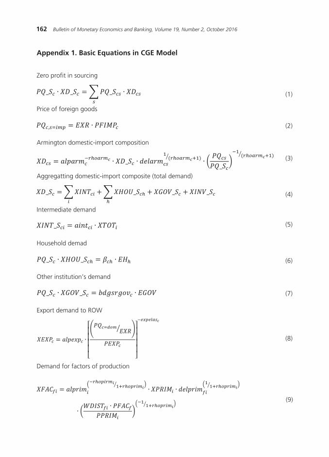
162 Bulletin of Monetary Economics and Banking, Volume 19, Number 2, October 2016
Appendix 1. Basic Equations in CGE Model
Zero profit in sourcing
Price of foreign goods
Armington domestic-import composition
Aggregatting domestic-import composite (total demand)
Intermediate demand
Household demad
Other institution’s demand
Export demand to ROW
Demand for factors of production
(1)
(2)
(3)
(4)
(5)
(6)
(7)
(8)
(9)
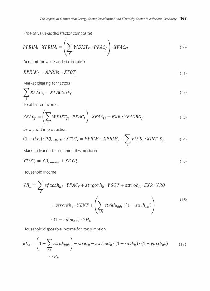
163The Impact of Geothermal Energy Sector Development on Electricity Sector In Indonesia Economy
Price of value-added (factor composite)
Demand for value-added (Leontief)
Market clearing for factors
Total factor income
Zero profit in production
Market clearing for commodities produced
Household income
Household disposable income for consumption
(10)
(11)
(12)
(13)
(14)
(15)
(16)
(17)
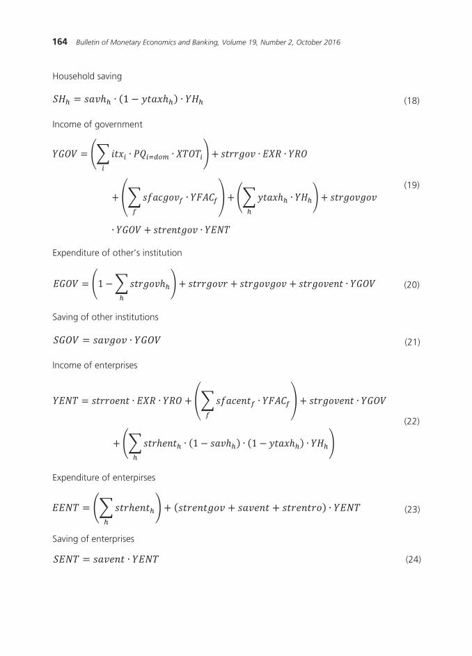
164 Bulletin of Monetary Economics and Banking, Volume 19, Number 2, October 2016
Household saving
Income of government
Expenditure of other’s institution
Saving of other institutions
Income of enterprises
Expenditure of enterpirses
Saving of enterprises
(18)
(19)
(20)
(21)
(22)
(23)
(24)

165The Impact of Geothermal Energy Sector Development on Electricity Sector In Indonesia Economy
Income of rest of the world (in ROW currency)
Expenditure of rest of the world (in ROW currency)
Aggregate saving
Aggregate investment
Investment demand
Consumer’s price index
(25)
(26)
1
1 1
1
(27)
(28)
(29)
(30)

166 Bulletin of Monetary Economics and Banking, Volume 19, Number 2, October 2016
Appendix 2. Equations for CO2 Emission in CGE Model
CO2 Emissions by industry
CO2 Emissions by household
National CO2 emissions
(31)
(32)
(33)
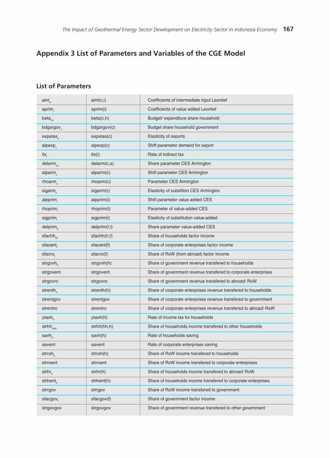
167The Impact of Geothermal Energy Sector Development on Electricity Sector In Indonesia Economy
aintci aint(c,i)
aprimi aprim(i)
betach beta(c,h)
bdgsrgovc bdgsrgov(c)
expelasc expelas(c)
alpexpc alpexp(c)
itxi itx(i)
delarmcs delarm(c,s)
alparmc alparm(c)
rhoarmc rhoarm(c)
sigarmc sigarm(c)
alpprimi alpprim(i)
rhoprimi rhoprim(i)
sigprimi sigprim(i)
delprimfi delprim(f,i)
sfachhhf sfachh(h,f)
sfacentf sfacent(f)
sfacrof sfacro(f)
strgovhh strgovh(h)
strgovent strgovent
strgovro strgovro
strenthh strenth(h)
strentgov strentgov
strentro strentro
ytaxhh ytaxh(h)
strhhhhh strhh(hh,h)
savhh savh(h)
savent savent
strrohh strroh(h)
strroent strroent
strhrh strhr(h)
strhenth strhent(h)
strrgov strrgov
sfacgovf sfacgov(f)
strgovgov strgovgov
Coefficients of intermediate input Leontief
Coefficients of value added Leontief
Budget/ expenditure share household
Budget share household government
Elasticity of exports
Shift parameter demand for export
Rate of indirect tax
Share parameter CES Armington
Shift parameter CES Armington
Parameter CES Armington
Elasticity of substition CES Armington
Shift parameter value added CES
Parameter of value-added CES
Elasticity of substitution value-added
Share parameter value-added CES
Share of households factor income
Share of corporate enterprises factor income
Share of RoW (from abroad) factor income
Share of government revenue transfered to households
Share of government revenue transfered to corporate enterprises
Share of government revenue transfered to abroad/ RoW
Share of corporate enterprises revenue transfered to households
Share of corporate enterprises revenue transfered to government
Share of corporate enterprises revenue transfered to abroad/ RoW
Rate of income tax for households
Share of households income transfered to other households
Rate of households saving
Rate of corporate enterprises saving
Share of RoW income transfered to households
Share of RoW income transfered to corporate enterprises
Share of households income transfered to abroad/ RoW
Share of households income transfered to corporate enterprises
Share of RoW income transfered to government
Share of government factor income
Share of government revenue transfered to other government
Appendix 3 List of Parameters and Variables of the CGE Model
List of Parameters
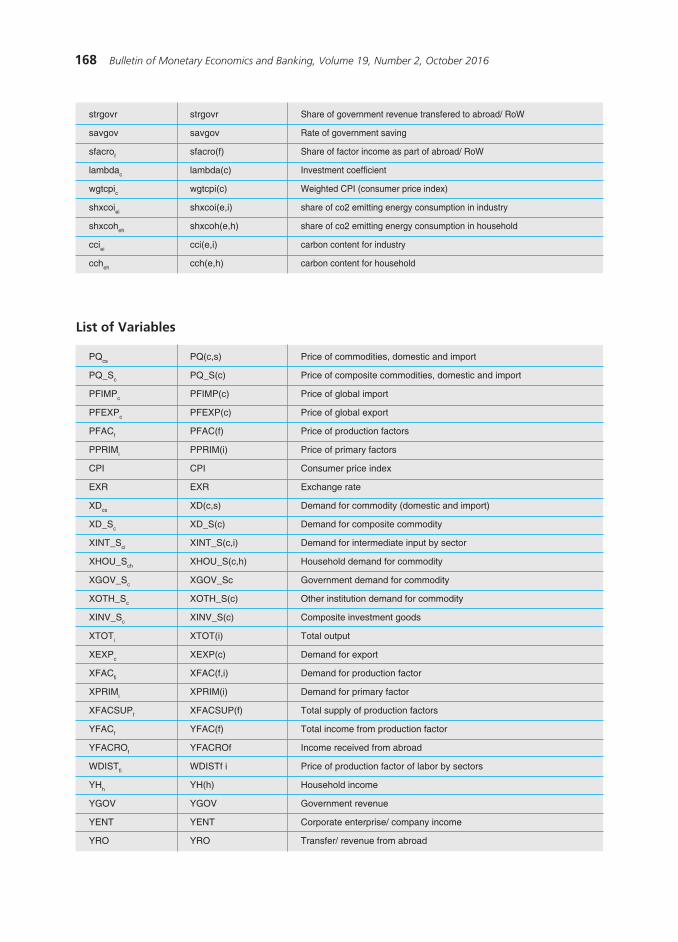
168 Bulletin of Monetary Economics and Banking, Volume 19, Number 2, October 2016
strgovr strgovr
savgov savgov
sfacrof sfacro(f)
lambdac lambda(c)
wgtcpic wgtcpi(c)
shxcoiei shxcoi(e,i)
shxcoheh shxcoh(e,h)
cciei cci(e,i)
ccheh cch(e,h)
PQcs PQ(c,s)
PQ_Sc PQ_S(c)
PFIMPc PFIMP(c)
PFEXPc PFEXP(c)
PFACf PFAC(f)
PPRIMi PPRIM(i)
CPI CPI
EXR EXR
XDcs XD(c,s)
XD_Sc XD_S(c)
XINT_Sci XINT_S(c,i)
XHOU_Sch XHOU_S(c,h)
XGOV_Sc XGOV_Sc
XOTH_Sc XOTH_S(c)
XINV_Sc XINV_S(c)
XTOTi XTOT(i)
XEXPc XEXP(c)
XFACfi XFAC(f,i)
XPRIMi XPRIM(i)
XFACSUPf XFACSUP(f)
YFACf YFAC(f)
YFACROf YFACROf
WDISTfi WDISTf i
YHh YH(h)
YGOV YGOV
YENT YENT
YRO YRO
Price of commodities, domestic and import
Price of composite commodities, domestic and import
Price of global import
Price of global export
Price of production factors
Price of primary factors
Consumer price index
Exchange rate
Demand for commodity (domestic and import)
Demand for composite commodity
Demand for intermediate input by sector
Household demand for commodity
Government demand for commodity
Other institution demand for commodity
Composite investment goods
Total output
Demand for export
Demand for production factor
Demand for primary factor
Total supply of production factors
Total income from production factor
Income received from abroad
Price of production factor of labor by sectors
Household income
Government revenue
Corporate enterprise/ company income
Transfer/ revenue from abroad
List of Variables
Share of government revenue transfered to abroad/ RoW
Rate of government saving
Share of factor income as part of abroad/ RoW
Investment coefficient
Weighted CPI (consumer price index)
share of co2 emitting energy consumption in industry
share of co2 emitting energy consumption in household
carbon content for industry
carbon content for household
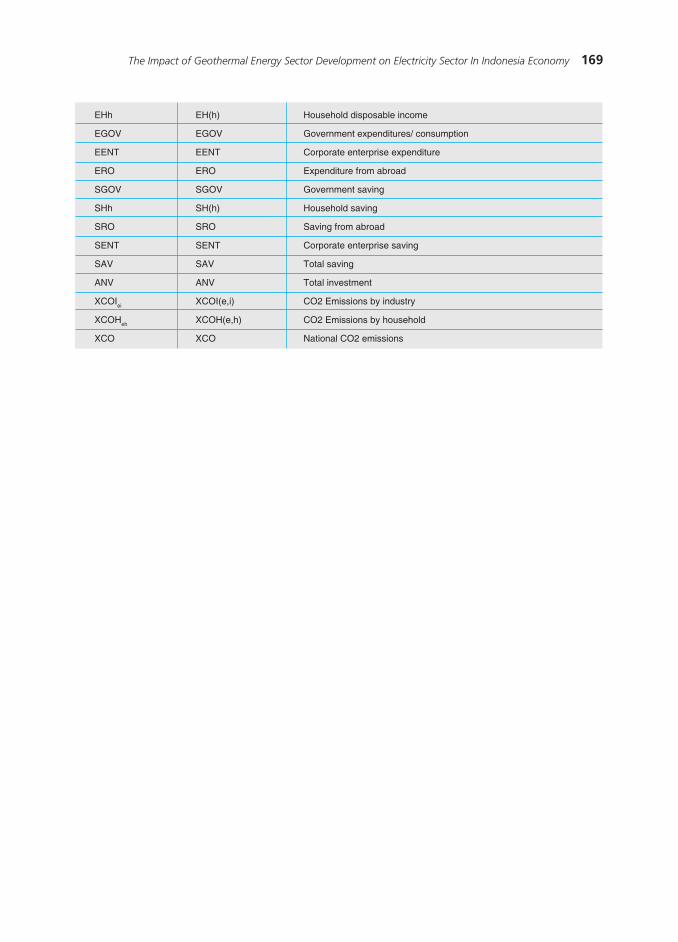
169The Impact of Geothermal Energy Sector Development on Electricity Sector In Indonesia Economy
EHh EH(h)
EGOV EGOV
EENT EENT
ERO ERO
SGOV SGOV
SHh SH(h)
SRO SRO
SENT SENT
SAV SAV
ANV ANV
XCOIei XCOI(e,i)
XCOHeh XCOH(e,h)
XCO XCO
Household disposable income
Government expenditures/ consumption
Corporate enterprise expenditure
Expenditure from abroad
Government saving
Household saving
Saving from abroad
Corporate enterprise saving
Total saving
Total investment
CO2 Emissions by industry
CO2 Emissions by household
National CO2 emissions

170 Bulletin of Monetary Economics and Banking, Volume 19, Number 2, October 2016
This page intentionally left blank
171Red Flags and Fraud Prevention on Rural Banks
RED FLAGS AND FRAUD PREVENTION ON RURAL BANKS
Ni Wayan Rustiarini 1 Ni Nyoman Ayu Suryandari 2
I Kadek Satria Nova 3
This paper identifies the effectiveness of the red flags in detecting fraudulent financial statements,
as well as preventive measures in appropriate to implement Rural Credit Banks (RCB). We use Field surveys
were used for RCBs in Bali Province, covering 60 indicators involving 101 internal auditors from 86 RCBs.
The result showed that capability is the most likely aspect (dimension) within the Fraud Diamond model to
influence fraudulent behavior. Efforts to prevent the fraud include cultivating a culture of honesty and high
ethics, evaluating the anti-fraud processes and control, and developing an appropriate oversight process.
Abstract
Keywords: Financial Risk, Liquidation, Corporate Governance, Audit
JEL Classification: G32, G33, G34, M420
1 Lecturer at Mahasaraswati Denpasar University ([email protected])2 Lecturer at Mahasaraswati Denpasar University ([email protected])3 Asisstant Lecturer at Mahasaraswati Denpasar University ([email protected])
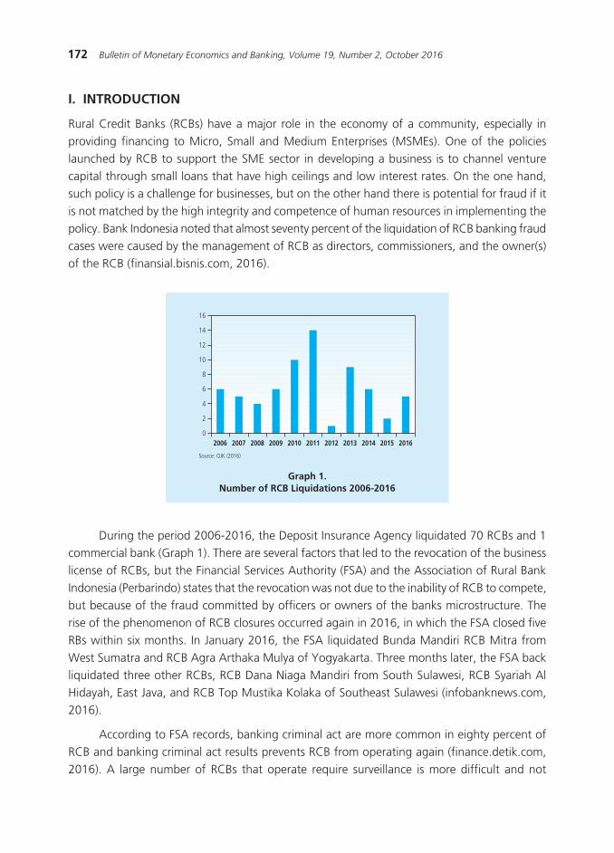
172 Bulletin of Monetary Economics and Banking, Volume 19, Number 2, October 2016
I. INTRODUCTION
Rural Credit Banks (RCBs) have a major role in the economy of a community, especially in providing financing to Micro, Small and Medium Enterprises (MSMEs). One of the policies launched by RCB to support the SME sector in developing a business is to channel venture capital through small loans that have high ceilings and low interest rates. On the one hand, such policy is a challenge for businesses, but on the other hand there is potential for fraud if it is not matched by the high integrity and competence of human resources in implementing the policy. Bank Indonesia noted that almost seventy percent of the liquidation of RCB banking fraud cases were caused by the management of RCB as directors, commissioners, and the owner(s) of the RCB (finansial.bisnis.com, 2016).
Graph 1. Number of RCB Liquidations 2006-2016
������������������
���� ���� ���� ���� ���� ���� ���� ���� ���� ���� �����
�
�
�
��
��
��
��
During the period 2006-2016, the Deposit Insurance Agency liquidated 70 RCBs and 1 commercial bank (Graph 1). There are several factors that led to the revocation of the business license of RCBs, but the Financial Services Authority (FSA) and the Association of Rural Bank Indonesia (Perbarindo) states that the revocation was not due to the inability of RCB to compete, but because of the fraud committed by officers or owners of the banks microstructure. The rise of the phenomenon of RCB closures occurred again in 2016, in which the FSA closed five RBs within six months. In January 2016, the FSA liquidated Bunda Mandiri RCB Mitra from West Sumatra and RCB Agra Arthaka Mulya of Yogyakarta. Three months later, the FSA back liquidated three other RCBs, RCB Dana Niaga Mandiri from South Sulawesi, RCB Syariah Al Hidayah, East Java, and RCB Top Mustika Kolaka of Southeast Sulawesi (infobanknews.com, 2016).
According to FSA records, banking criminal act are more common in eighty percent of RCB and banking criminal act results prevents RCB from operating again (finance.detik.com, 2016). A large number of RCBs that operate require surveillance is more difficult and not
173Red Flags and Fraud Prevention on Rural Banks
4 Henceforth, called EO Internal Audit
simultaneous as applied to commercial banks. Not surprisingly, the potential for fraud in RCBs is higher than commercial banks. A tight banking monitoring system can lead to detection of fraud so that it can be resolved internally and not be detrimental to the customer. Reflecting on this phenomenon, RCBs need to have an internal reliable monitoring system.
Although cases of fraud occurring in the RCBs are far more than the commercial banks, until now the government has not issued regulations requiring RCBs to have anti-fraud strategy. To reduce the chances of irregularities of alleged banking fraud provisions, the FSA issued Regulation No. 4 / POJK.03 / 2015 on the Application of Governance for RCB which came in effect March 31, 2015. The Regulation confirms the obligation to implement RCB governance principles in all business activities at all levels of the organization. One form of implementation of good governance is to streamline the internal audit function as part of the RCB Internal Control System (ICS). FSA Circular Letter No. 7 / SEOJK.03 / 2016 of the RCB Internal Audit Standards stated that in conducting surveillance operations that include planning, implementation, and monitoring of audit results, Chief Executive Officer and the Board of Commissioners is to be assisted by the Internal Audit Unit (IAU) or Executive officers (EO) of the Internal Audit4.
Fraud detection task is not an easy task. The IAU or EO Internal Audit require indicators or signs (red flags) that can assist in focusing performance when scanning the financial statements. Red flags are potential symptoms that indicate a higher risk of an intentional misstatement in the financial statements. Despite the red flags being regarded as an early warning alarm (early
warning signal) which can reduce the risk of detecting fraud, further in depth audit investigation is required to obtain accurate results. Based on the concept of The Fraud Triangle, Statement
on Auditing Standard No. 99 requires the external auditor to use 42 red flags when detecting fraudulent financial statements. Several previous studies have been conducted to identify the effectiveness of the use of red flags based The Fraud Triangle in detecting fraud (Albrecht and Romney, 1986; Pincus, 1989; Heiman-Hoffman et al., 1996; Moyes et al., 2006; Omar, 2011; Rustiarini and Novitasari, 2014). This study intends to develop the results of previous studies using the new concept of The Fraud Diamond.
The purpose of this study to identify the effectiveness of red flags in the financial statements of banking fraud detection, especially RCB. The IAU or EO Internal Audit also identified fraud prevention measures that are believed to be appropriate to implement with RCBs. RCB banking sector fraud is systemic, and its impact can extend to other similar banks or even to the banking system as a whole. Fraud in some rural banks certainly has a negative impact across the industry, and if not addressed, could reduce public confidence in the bank. Thus it is a necessary proactive measure of the Internal Audit Unit or EO Internal Audit to determine the indicators, as well as the prevention and detection of accounting fraud.
174 Bulletin of Monetary Economics and Banking, Volume 19, Number 2, October 2016
This study uses a questionnaire survey of the IAU or EO as a function of the Internal Audit responsible for internal controls at the internal control system of the RCB. This study provides a theoretical contribution to supplement the results of previous studies which use the concept of The Fraud Triangle. The cornerstone of the different theories used in this research is The Fraud
Diamond which considers all the individual factors on individuals as perpetrators of fraud. Results of this research are expected to provide input when formulating policy or anti-fraud strategy on RCB, as has been applied to commercial banks. Previous Bank Indonesia issued Circular No. 13/28 / DPNP of 2011 on Anti-Fraud Strategy Implementation for Commercial Banks requiring any commercial banks to have an anti-fraud strategy that is comprehensive and detailed to reinforce the bank statistics (Indonesian Banking Statistics, IBS). But until now there has been no similar regulation issued by the government for RCBs particularly where cases of fraud are more common with RCBs than commercial banks. Thus, the study is important and interesting to do to be able to formulate indicators of fraud detection and the steps needed to prevent fraud.
The first part of this paper is an introduction outlining the background and purpose of the study. The second part to reviews the theories related to the model, i.e. The Fraud Diamond as the foundation for the development of indicators of fraud detection. The third part reviews the methodology, and the fourth part of this paper presents the results and analysis. Conclusions and suggestions are presented in the last section.
II. THEORY
2.1. The Fraud Diamond
The theory used as the basis of this research is Theory of Fraud Diamond. Before this concept was widely introduced, the Association of Certified Fraud Examiners use The Fraud Triangle model proposed by Cressey (1950, 1953) as an initial foundation in various studies on cheating. The concept of the fraud triangle emphasized three elements of the causes of fraud, i.e. pressure or incentive, chance (opportunity), and rationalization. The Fraud Diamond introduced by Wolfe and Hermanson (2004) adds the ability (capability) as the fourth element. The rationale underlying this concept is that cheating does not happen without the right people, the right position, and would have to have the right skills.
The first element, pressure, is a condition where a person accepts the demands, both financial and non-financial, making it more vulnerable to cheating (Choo and Tan, 2007). In financial terms, stress occurs when management needs money to meet personal needs such as an economic stress in the family or lifestyle (Rustendi, 2009). Non-financial pressure occurs when financial targets beyond the ability of management, compensation, incentives, or career paths in line with expectations, as well as the failure of the working relationship between the employee and the employer (Moeller, 2009) so as to change behavior to be more inclined to cheating.
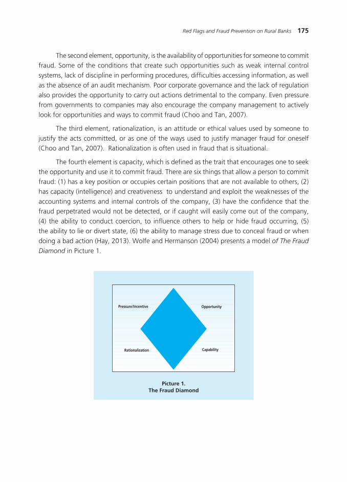
175Red Flags and Fraud Prevention on Rural Banks
The second element, opportunity, is the availability of opportunities for someone to commit fraud. Some of the conditions that create such opportunities such as weak internal control systems, lack of discipline in performing procedures, difficulties accessing information, as well as the absence of an audit mechanism. Poor corporate governance and the lack of regulation also provides the opportunity to carry out actions detrimental to the company. Even pressure from governments to companies may also encourage the company management to actively look for opportunities and ways to commit fraud (Choo and Tan, 2007).
The third element, rationalization, is an attitude or ethical values used by someone to justify the acts committed, or as one of the ways used to justify manager fraud for oneself (Choo and Tan, 2007). Rationalization is often used in fraud that is situational.
The fourth element is capacity, which is defined as the trait that encourages one to seek the opportunity and use it to commit fraud. There are six things that allow a person to commit fraud: (1) has a key position or occupies certain positions that are not available to others, (2) has capacity (intelligence) and creativeness to understand and exploit the weaknesses of the accounting systems and internal controls of the company, (3) have the confidence that the fraud perpetrated would not be detected, or if caught will easily come out of the company, (4) the ability to conduct coercion, to influence others to help or hide fraud occurring, (5) the ability to lie or divert state, (6) the ability to manage stress due to conceal fraud or when doing a bad action (Hay, 2013). Wolfe and Hermanson (2004) presents a model of The Fraud
Diamond in Picture 1.
Picture 1.The Fraud Diamond
������������������
����������
����������
��������������
176 Bulletin of Monetary Economics and Banking, Volume 19, Number 2, October 2016
2.2. Fraud
The term fraud is inseparable from the development of the business world. The issues of bribery, embezzlement, money laundering, and theft of product are just a few examples of a number of cases that have occurred. Statement of Auditing Standards # 99 defines fraud as an intentional act to produce a material misstatement in the financial statements. Tuanakotta (2010) suggests fraud as a deliberate action to do or not do something properly so that enterprises can publish the financial statements materially misleading users. Cheating can be grouped in three forms, namely misappropriation of assets (asset misappropriation) accounting fraud or fraudulent financial statements (statement of financial fraud), and corruption.
In the world of banking provisions, the definition of fraud was stipulated in Circular No. 13/28 / DPNP 2011 the Anti-Fraud Strategy Implementation for Commercial Banks. Fraud is said to be an act of irregularities or omissions deliberately done to deceive, cheat, or manipulate the bank, customers or other parties that happen in the Bank and / or by means of the Bank resulting in losses suffered by the bank, customers or other parties, either directly or indirectly. Three groups of acts of fraud are common in the banking world, i.e. distortion associated with the provision of credit (43%), manipulation (19.6%), and forgery (18.6%). Other unethical actions that can be categorized as fraud is embezzlement, abuse of authority, abuse of ATM and PIN, as well as the misuse of customer funds (FSA, 2016). The number of offenders who allegedly commit bank crime (banking criminal acts) involved shareholders as one group, where as many as seven directors, executive officers, as many as ten people, and one bank employee.
The economic crisis also increased the chances of fraud in some countries. One of three companies worldwide reported themselves as victims of fraud during the past 12 months (Gillentine, 2009), similar to the results of a survey conducted by PricewaterhouseCoopers (PwC 2009) where it was reported that 30% of respondents claimed to have experienced fraud. KPMG (2009) also found that 65% of the companies’ executives said that cheating is a risk that often occurs in their company. In connection with the perpetrators of fraud, a study conducted by Wolfe and Hermanson (2004) revealed that most of the fraud committed by a company. This fact reinforces the Ernst and Young survey, which concluded that 82% of respondents said their employees were involved in the fraud, and 28% were involved in management (Wolfe and Hermanson, 2004).
This condition is not much different from the case of banking fraud that occurs in Indonesia. LPS had liquidated five RCBs during the first five months of 2016. This number continues to increase the possibility of up to seven or eight RCBs to the end of the year (business keuangan.kompas.com, 2016). Although there are several factors that cause revocation of RCBs, the main cause of the closure was due internal conditions such as unhealthy RCB fraudulent practices. RCB administrators often seem to forget the prudential banking provisions to the extent there is the irresponsible public funds. Abuse of authority by a RCB manager triggers other problems such as poor financial performance. This phenomenon is emphasized as most
177Red Flags and Fraud Prevention on Rural Banks
of the fraud is committed by internal party managers such as directors, commissioners, and the owner(s) of RCBs. Although there are customers who commit fraud, certainly it cannot be separated often there is from some form of support from a person within the company. Hence, there is a need for a reliable and adequate internal control system.
2.3. Fraud Indicators (Red Flags)
Detecting fraud is not an easy thing for an auditor. Although cases of cheating is not a foreign thing in the business world, often the internal and external auditors are not able to disclose a case. Often cheating is packaged such that the auditor would have difficulty to detect misstatements. The Association of Certified Fraud Examiners (ACFE 2010) stated that internal auditors can detect only 13.7% of cases of fraud occurring, while the external auditors have a lower number that is equal to 4.2% of the total cases reported. This condition contradicts the results of a survey conducted by two large public accounting firms, i.e., KPMG and PricewaterhouseCoopers in Malaysia in 2009, which showed that in fact before financial fraud cases occurred, the auditor may detect fraud through indicators (red flags). However, the auditor often ignore the presence of red flags or even them “pushed under the carpet” on-demand from a company that is a victim of fraud. Various reasons are used to ignore such indicators such as maintaining the company’s reputation, market potential, and employee motivation. The company also used the excuse of “the amount is too small to affect the company” (Omar and Din, 2010). Thus, the auditor deliberately did not reveal the fraud indicators in the audit report, or did not discuss it with the company’s management.
Groveman (1995) in an article that focuses on the detection of misstatements of financial statements reveals that often the cause of failure of the audit is the audit team’s imprecise reaction to various warning signals. Auditors should understand this signal and act correctly according to the instructions given by such signals. Indicators of misstated financial statements include the existence of overstatements in recording inventory, an aggressive application of accounting principles, inaccurate revenue recognition, inadequate loss reserves, understatement in recording costs and fees, and the existence of unusual transactions with related parties. A major signal can be a complicated organizational structure, partnership or joint venture that is unusual, and the change of auditor (Friedman, 1995). Other signs of fraud can be dishonesty of managers to auditors, frequent disputes between managers and auditors, the desire of managers to achieve the target or benefit from existing projects, as well as the wishes of the client for approval (Opinion shopping) (Heiman-Hoffman et al., 1996) ,
If the indicators are visible when the client’s financial statements audited, the auditor should be skeptical and investigate further to ensure there is no fraud, so as not to cause a material misstatement in the financial records. If there is something suspicious, these indicators help auditors to focus on performance in conducting fraud risk assessment.
178 Bulletin of Monetary Economics and Banking, Volume 19, Number 2, October 2016
2.4. Cheating Effectiveness Indicators (Red Flags)
Statement on Auditing Standard No. 99 requires the external auditor to use 42 red flags in detecting fraudulent financial reporting (Moyes et al., 2006). Indeed, any red flags have different levels of effectiveness in detecting fraud. Differences in the assessment is due to differences in perception (Apostolou et al., 2001; Moyes, 2007), personal characteristics that assess (Robbins and Judge, 2008), incentives (Messier et al., 2005), or differences in the activities and responsibilities associated with work (Gullkvist and Jokipii, 2013). Even individuals who are in the same profession, internal auditors and external auditors also have different perceptions of the effectiveness of red flags.
Internal auditors are usually motivated to identify the causes of fraud and ensure effective internal control in the company to prevent fraud (Norman et al., 2011). Management must decide whether to develop additional control systems for a number of conditions that have not been resolved. In this case the management needs to do a cost-benefit analysis of risk versus the cost of controlling or reducing the risk mitigation benefits of the (PwC 2004). Internal auditors are trying to prevent adverse outcomes of the company so they tend to account for a favorable cost benefit analysis of the company. One important thing to keep in mind is that the internal control system will not be effective for fraud made by top management because they will not allow internal auditors to investigate fraud committed. In this condition, it is necessary involve the board of directors, audit committee and external auditors.
The external auditor role is to reveal the fraud that occurs due to low system of internal control and fraud committed by top management. In determining the effectiveness of red flags, the auditor has a different view of the materiality because it is determined by the different incentives (Messier et al., 2005), although there are no standard guidelines regarding the amount threshold cut off of materiality (Blokdijk et al., 2003). The external auditor is to report any differences or material deviation, or decide whether an item is material or not, which will depend on the assessment of the risk of fraud.
Research on the perception of the external auditors and internal auditors on the effectiveness of red flags has been tested using the concept of The Fraud Triangle (Albrecht and Romney, 1986; Pincus, 1989; Kaplan and Reckers, 1995; Heiman-Hoffman et al., 1996; Weiseborn and Norris, 1997; Moyes et al., 2006; Hegazy and Kassem, 2010; Omar, 2011; Yang et al., 2009; Moyes and Baker, 2009; Moyes et al., 2013; Gullkvist and Jokipii, 2013; Rustiarini and Novitasari, 2014), as well as indicators of fraud risk management (Coram et al., 2008; Liou, 2008). The findings demonstrate the various outcomes related to the importance of indicators in assessing the risk of fraud.
Prior to the Enron case, the use of red flags in carrying out the audit was not an important, as can be seen from some of the earlier studies. Albrecht and Romney (1986) revealed that the red flags are only used when there is cheating, and when fraud does occur then the red flags would not be helpful. Pincus (1989) also revealed that these indicators only serve to complement
179Red Flags and Fraud Prevention on Rural Banks
and uniform audit methods, but it does not help in predicting and assessing the risk of fraud, and only effects the reporting of a limited number of cases (Kaplan and Reckers, 1995). Similar results were disclosed by Weiseborn and Norris (1997) that highlighted the use of red flags were not valid for detecting fraud caused by management, but is more appropriately used to detect non-management fraud.
The study results where contradictions began to emerge from the Enron case further revealed the importance of red flags in detecting fraud. American Institute of Certified Public
Accountant (2002) reported that indeed there are 16 red flags were clearly visible before the fall of Enron. This statement is a reminder to the auditor profession to keep using a list of red flags in performing their duties. This statement has the support of the majority of respondents in the study done by Koornhof and Plessis (2000) which states that red flags are helpful in assessing the risk of fraud and provide early information about potential fraud. Several other researchers (Hegazy and Kassem, 2010; Moyes et al., 2006) also claimed that the red flags are effective for use in detecting fraud. Consistent with previous research results, the findings of Jokipii and Gullkvist (2013) also showed that internal auditors felt the importance of detecting red flags associated with the misuse of the assets of those associated with fraudulent financial reporting.
Over time, regulators and academics that focus on methods of detection and prevention of fraud have developed a new indicator of fraud. Referring to the progress of science, the research developed the results of previous studies using the new concept of The Fraud Diamond. This concept is used because it characterizes actual fraudulent behavior - it is not enough if only based on pressure, opportunity or rationalization. The most important thing that must be owned by the actor of cheating is sufficient ability to combine these three factors into a real action.
2.5. RB Internal Control System
FSA Circular Letter No. 7 / SEOJK.03 / 2016 of the Internal Audit Standards RB stated that the system of internal control is a control mechanism that is built to safeguard and secure the assets of RCBs, reduce the impact of losses including fraud, enhance organizational effectiveness, and is expected to increase cost efficiency. Internal audit function is part of the internal control system and is any activity related to auditing and reporting of audit results regarding the implementation of the control system in a coordinated manner within each level of management. The scope of internal control of the RCB includes aspects that are able to ensure the safety of the funds held by the public and other third parties. To achieve transparency and clarity, an internal audit is required to support the creation of an effective internal control system.
Implementing an internal audit is the role of the IAU or EO Internal Audit in assisting the Director and the Board of Commissioners to supervise RCB operations that includes planning, implementation, and monitoring of the audit results. The IAU or EO Internal Audit analyses and assesses the areas of finance, accounting, operations, and other activities at least by way
180 Bulletin of Monetary Economics and Banking, Volume 19, Number 2, October 2016
of direct examination and analysis of documents, as well as to provide recommendations for improvements and information on the activities examined at all levels of management. The IAU or EO Internal Audit should also be able to identify all possibilities to improve and increase the efficient use of resources and funds.
The organizational structure of the internal audit function is formed in accordance with the amount of core capital referred to in Article 59 of the FSA Rules Governing RCB that include:
1. A RCB with core capital of at least USD 50,000,000,000.00 (fifty billion rupiah) shall establish an Internal Audit Unit (IAU); or
2. A RCB with a core capital of less than Rp. 50,000,000,000.00 (fifty billion rupiah) shall appoint one (1) person Executive Internal Audit.
In addition to the various regulations, in the first quarter of 2016, a study was published on the RCB Based Surveillance of Risk (Risk Based Supervision -RBS). This study was made to develop RCB monitoring methods effective and efficient so that it grows well and contribute to the economy of the people, especially in the region where the RCB is located. In order to improve the Capacity Building Supervisor RCB, socialization was conducted the first quarter of 2016 regarding changes in the RCB system of supervision based on RCB compliance (compliance-
based supervision), and based on risk (risk based supervision). This activity is the first step to introduce risk-based supervision of rural banks to the supervisor RCBs, noting that this change requires a paradigm shift from compliance-based supervision to risk based supervision, and while introducing stages that will require supervisors to implementing a risk based supervision cycle (FSA, 2016).
III. METHODOLOGY
This study is a survey of the all RCBs in Bali Province. There are several considerations that underlie the research locations. First, the FSA Regional VIII Bali -Nusa Southeast general noted that RCBs in Bali province have good performance, especially for the period December 2014 to October 2015, but no doubt there are still some weaknesses that should be corrected as RCB capital reinforcement, improvement of quality sustainable human resource, and the implementation of RCB good governance (bali.bisnis com, 2016). Secondly, the Economic Studies and Regional Financial Quarter 2016 reports published by Bank Indonesia show an increase in the ratio of Non Performing Loan (NPL) or bad loans for RCBs in Bali province at 4.75%, which increased to 5.75% by September 2016 (Radar Bali, 2016). This Graph exceeds the limit specified by NPL FSA at 5%. This condition was caused by rapid price increases in the sectors of construction, trade, accommodation, and real estate in Bali that resulted in saturated rates. The expectation
gap caused investors to do business using bank credit which delays payment of credit (bali.tribunnews.com, 2016). Not infrequently, the case of bad credit is a source of the banking criminal acts. FSA data shows that of 26 cases of banking criminal acts that occurred, 55% were caused by the case of credit (finance.detik.com, 2016).

181Red Flags and Fraud Prevention on Rural Banks
Third, the performance of RCBs in Bali Province is closely related to the presence of Village Credit Institutions (VCIs) as microfinance institutions located in all customary villages in Bali. In this case, the number of VCIs reached 1,466 to become competitors with RCBs in lending. Moreover, VCI credit terms are easier, with faster disbursement of funds, and have an unsecured credit facility of certain values with communities in traditional villages where the VCI is operational. This high level of competition caused RCB employees to tend to ignore the procedures and conditions of lending in order to chase their target alone (beritadewata.com, 2016). Some of the acts of fraud committed a bank officer include over finance credit, record keeping supporting documents fake of credit proposals, and other fraud carried out by the debtor, the third party, as well as the bank itself (Radar Bali, 2016). Helping redress these events is the basis for the research on RCB in Bali Province.
Collecting data used a questionnaire to determine the employees’ perception of the Internal Audit or EO Internal Audit on the effectiveness of red flags in the financial RCB statements for detecting fraud, and to identify the necessary efforts in the prevention of fraud. Given the role mandated to employees of the IAU or EO Internal Audit have the same functionality as the internal auditor, this study will use the term internal auditor to replace the term “employees of the IAU or EO Internal Audit. Based on data obtained from Perbarindo Bali to 2016, there were 138 rural banks spread over 9 (nine) regencies and municipalities in Bali. A total of 44 RCBs does not have an internal auditor, but there are also some banks that have an internal auditor with more than one person. There are eight RCBs that did not participate in this study by reason of routine business, FSA checks, a change of leadership, building renovation, and leadership barring participating in the study (Graph 2). In all, 86 rural banks that participated in this study. The survey period ranged from June 2016 to September 2016. The number of internal auditors willing to fill in the questionnaire totaled 101 people from 86 RCBs.
Graph 2.RCB Participation Rate
�����������
������������������������������� ���������� ��������������������������� ���������� ������������������������������� ����

182 Bulletin of Monetary Economics and Banking, Volume 19, Number 2, October 2016
The questionnaire used in this study consists of three parts. The first part contains questions about respondents’ demographic information, the second part contains a list of fraud indicators (red flags) by the auditor, and the third section contains the necessary steps in order to prevent fraud. The indicators used are in accordance with Statement of Auditing Standard 99, were adapted from the research of Moyes (2006) and Omar (2011). It was further adapted to the conditions in Indonesia. Fraud indicators are grouped in four dimensions that correspond with The Diamond Fraud namely: (1) the pressure as represented by 13 indicators, (2) an opportunity as represented by 27 indicators, (3) rationalization / attitude as represented by 15 indicators, and (4) ability as represented by 5 indicators. A total of 60 indicators were used. Respondents were asked to give an opinion on the effectiveness of red flags to detect fraud using a four-point scale: 1 = Very Ineffective, 2 = Not Effective, 3 = Effective, and 4 = Very Effective.
The fourth section lists the fraud prevention measures in accordance with SAS 99 Exhibit “Management Anti-Fraud Programs and Controls Guidance to Help Prevent, Deter, and Detect
Fraud “. There are 14 types of actions that are grouped into three main categories, namely creating a culture of honesty and high ethics, evaluating the process and control strategy of anti- fraud, and developing appropriate monitoring processes. Respondents were asked to identify the effectiveness of the preventive measures using a four-point scale: 1 = Very Ineffective, 2 = Not Effective, 3 = Effective, and 4 = Very Effective. Researchers compared the effectiveness of each group of red flags that are categorized by the Fraud Diamond. This study uses average values (mean) totals for each group of red flags assessed based on the perception of the internal auditor. Furthermore, each group indicators will be ranked and presented based on Five Big Red Flags of “Highly Effective” categories for Pressure / Incentive, Opportunity, Rationalization, and Capability.
In addition, this study also analyzes the influence of the demographic characteristics of the external auditor on the perception of the effectiveness of red flags in detecting fraud. Data were analyzed using multiple linear regression, which had previously tested the classical assumption of the normality test, multicollinearity, and heteroscedasticity test. Furthermore, the feasibility test models includes a test of determination (R 2), F test and t test. The determination test is used to measure the ability of the model to explain variations in the dependent variable. F test is used to determine the effect of simultaneous independent variables on the dependent variable, while the t-test is used to determine the effect of partially independent variables on the dependent variable (Ghozali 2011). The independent variables are the demographic characteristics of respondents as measured by gender, age, education level, and years of experience in detecting fraud, as well as training or seminar experience in the fraud detection. The independent variable is the effectiveness of red flags in detecting fraud.

183Red Flags and Fraud Prevention on Rural Banks
IV. RESULTS AND ANALYSIS
4.1. Detailed Results of the Questionnaire
This study uses primary data obtained directly by visiting each RCB where questionnaires were provided equal to the number of internal auditors in the RCBs. The time period given to complete and return the questionnaires was a maximum of 60 days from the date the questionnaire was given to each respondent. Number of questionnaires distributed totaled 101 questionnaires, and the rate of return (response rate) was 100%. Of the 101 questionnaires returned, there are two questionnaires that couldn’t be used in the analysis because not all items of the questionnaire were completed. Thus, a number 99 questionnaires were processed (see Table 1)
�������������������������������������������������������������������������������������������� �������������� ������������������������������������������� ��������
�������������������������������������� ����
�������� �����
��������������������� ���������
����
�������
���
4.2. Characteristics of Respondents
The first step in analyzing the questionnaire is to identify the characteristics of the internal auditors on the basis of gender, age, education level, years of experience in detecting fraud, as well as the internal auditor’s participation in training or seminars on the detection of fraud (see Table 2).
�������� ������ ����������� ���� ����� ������ ���� ����� ����� ���� ���������������������� ������������ �� ����� ��� ��� ������������������ ������������� ������ ����� ����� ������������� ������ ��������������������������� ����� �������� �����������������������������������������������������������
������������������������������� �� ��
�����������
������������ ������� ��������
�
��
��
�
��
��
��������
������������������������
�������������������������
�
�����������������
����������
������������
������������
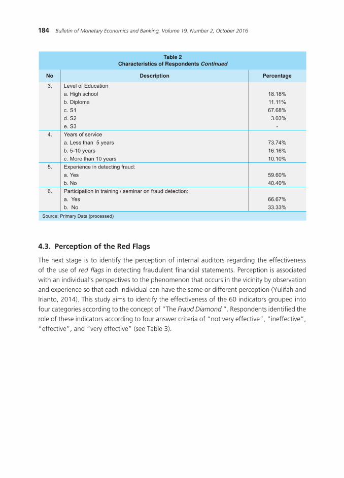
184 Bulletin of Monetary Economics and Banking, Volume 19, Number 2, October 2016
4.3. Perception of the Red Flags
The next stage is to identify the perception of internal auditors regarding the effectiveness of the use of red flags in detecting fraudulent financial statements. Perception is associated with an individual’s perspectives to the phenomenon that occurs in the vicinity by observation and experience so that each individual can have the same or different perception (Yulifah and Irianto, 2014). This study aims to identify the effectiveness of the 60 indicators grouped into four categories according to the concept of “The Fraud Diamond “. Respondents identified the role of these indicators according to four answer criteria of “not very effective”, “ineffective”, “effective”, and “very effective” (see Table 3).
�������� ������ ����������� ���� ����� ������ ���� ����� ����� ���� ���������������������� ������������ �� ����� ��� ��� ������������������ ������������� ������ ����� ����� ������������� ������ ��������������������������� ����� �������� �����������������������������������������������������������
������������������������������� �� ��
�����������
������������ ������� ��������
�
��
��
�
��
��
��������
������������������������
�������������������������
�
�����������������
����������
������������
������������
������������������������������� �� ������������
����������� ������������
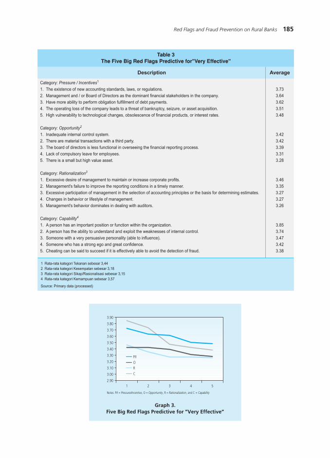
185Red Flags and Fraud Prevention on Rural Banks
��������������������������������
�� ����������� ���������� �������������������������������������� ������������������������������� ������������������������� ����������������������� ��������� ������������������������������������������������������������������� � �������������������������� ���������������������������������� �������������������� ����������� ����������������������� ������� ��� ��������������� �� ���������� ������� ����������������������
����������������������
�� ������������������ ���������������� ������������������������� �������������������������� ��������������� ��������������� ������������������������������ ����������������� ���� � �� ����� ������������������������������� ������������������������������������
���������� �������������
�� �� �������������������������������������������� ������ ������������������� ��������������������������������������������� ������������������������������ �� ������������ ��������������������������������� ��������� ����������� �������������������������������������������� � ������������������������������������������������� �����������������������������������������������������
���������������������
�� ���������������������������������������� ������������������������������ �������������������������������������������������������������������������� ��������� ��������������������������������������������������������� ��� � �������������������������������������� ������ ���� ��������� �������������� ���������������� ��������������������������� ������������
����������������������������������� ���������������� ����
�����������
��� ������������������� �����
������� ���������� �
�� ��� �������������
�� �����������������
������� �� ��� �����
�������
���������������������������������������� ��������������������������������������������������������������������������������������������������� ������������������������������������������
Graph 3.Five Big Red Flags Predictive for ”Very Effective”
����
����
����
����
����
����
����
����
����
����
����
� � � � �
������
� ��������������������������������������������������������� ���������������������� ���
186 Bulletin of Monetary Economics and Banking, Volume 19, Number 2, October 2016
With regard to the average level for the score of effectiveness, it can be concluded that the fraud indicators (red flags) meet the effective criteria for use in detecting fraud. Analysis of respondents’ answers indicate that the dimension of the Fraud Diamond that has the highest average value is the ability (capability) (Graph 3). The results of this study reinforce the Theory of Fraud Diamond which stresses that the ability of a person plays an important role when in the occurrence of fraud. Even though a person has the motivation, opportunity, and rationalization, but if the person does not have the ability to carry out or conceal the fraud then cheating is not possible. It is likened to a door, an opportunity is a way to open the door, then the pressure (incentive) and rationalization of guiding one toward the door, but only capability allows one to recognize the open door as an opportunity. Another important point is that only people who have a high capacity would understand well the internal control system, identify weaknesses, and how to use it for a fraud. Someone must have the skills and abilities when it comes cheating. Respondents in this study support the argument of Wolfe and Hermanson (2004) that although a person feels pressure, opportunity and rationalization, fraud is not possible without the presence capability.
When compared with the results of previous studies conducted by Moyes et al. (2006) to determine the perception of internal auditors, the results showed that the category of opportunity and rationalizations were more effective in detecting fraudulent financial reporting compared to the category of pressures / incentives. Subsequent research by Yang et al. (2009) on the external auditors and internal auditors revealed that the indicators for categories of pressures and opportunity were more effective than the category of rationalization, while research by Moyes et al. (2013) saw the category of opportunity as most effective compared to two other indicators.
Perception of internal auditors in determining the effectiveness of red flags must not be separated from the influence of the demographic characteristics of the internal auditor. Demographic characteristics such as gender, age, education, years of experience of detecting fraud in an audit, as well as training or seminars related to the detection of fraud, would establish the competence of internal auditors so that they can carry out tasks with precise detection. The association has been demonstrated by the results of tests performed using multiple linear regression analysis as presented in Table 4. Previous research met the classical assumption that it can be continued on multiple linear regression test.
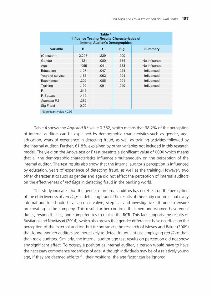
187Red Flags and Fraud Prevention on Rural Banks
Table 4 shows the Adjusted R 2 value 0.382, which means that 38.2% of the perception of internal auditors can be explained by demographic characteristics such as gender, age, education, years of experience in detecting fraud, as well as training activities followed by the internal auditor. Further, 61.8% explained by other variables not included in this research model. The yield on the Anova test or F test presents a significant value of 0000 which means that all the demographic characteristics influence simultaneously on the perception of the internal auditor. The test results also show that the internal auditor’s perception is influenced by education, years of experience of detecting fraud, as well as the training. However, two other characteristics such as gender and age did not affect the perception of internal auditors on the effectiveness of red flags in detecting fraud in the banking world.
This study indicates that the gender of internal auditors has no effect on the perception of the effectiveness of red flags in detecting fraud. The results of this study confirms that every internal auditor should have a conservative, skeptical and investigative attitude to ensure no cheating in the company. This result further confirms that men and women have equal duties, responsibilities, and competencies to realize the RCB. This fact supports the results of Rustiarini and Novitasari (2014), which also proves that gender differences have no effect on the perception of the external auditor, but it contradicts the research of Moyes and Baker (2009) that found women auditors are more likely to detect fraudulent use employing red flags than than male auditors. Similarly, the internal auditor age test results on perception did not show any significant effect. To occupy a position as internal auditor, a person would have to have the necessary competence regardless of age. Although individuals may be of a relatively young age, if they are deemed able to fill their positions, the age factor can be ignored.
���������������������������������� ����������������
������������������������� ���
������������������������
��������������������������������������������������������������������������������������
�������� � � ��� �������
����� �� �������������������������������
��������������������������
�������������������������
����������������������������������������������������������������
188 Bulletin of Monetary Economics and Banking, Volume 19, Number 2, October 2016
The demographic characteristics of the tenure of the internal auditor affects the perception of the effectiveness of red flags , which supports the research of Hegazy and Kassem (2010) that found the auditor’s tenure affected the fraud detection using red flags. The longer the time a person holds office as an internal auditor, of course, will increase the knowledge and expertise. Longer working lives will also provide an opportunity for internal auditors to deeply explore their capabilities and excel, including enhancing their capabilities associated with the detection of fraud. Long working lives will also enable internal auditors develop their potential. When linked with the auditor’s perception of the effectiveness of red flags in detecting fraud, the longer the internal auditor’s tenure, the more effective s/he would be in identifying red
flags that can be used in detecting fraud.
Often the level of formal education of a person is used as a measure of the level of knowledge of the person. To be able to work as an internal auditor, a person would need specialized education, especially in the field of accounting. The higher the education the more extensive the auditor’s knowledge so as to positively affect decision-making abilities, one of which relates to the determination of the effectiveness of red flags in detecting fraud. Auditors who have a master degree in accounting or business would likely increase the use of red flags to detect fraud, compared to an auditor who does not have a degree at all (Moyes and Baker, 2009). The results support the results of research of Yang et al. (2009) and Rustiarini and Novitasari (2014), which indicates that the education of the external auditor has an effect on the effectiveness of fraud detection.
The purpose of this research is to detect fraud from previous assignment experiences. In connection with the demographic characteristics of experience in detecting fraud, the results of this study suggest that the experience is the most significant variable that has an effect on the perception of internal auditors on the effectiveness of red flags. Experienced internal auditors will be able to recognize items in the financial statements that are often abused, and have an accurate argument for the findings (Libby and Frederick, 1990). Experience would help auditors choose the appropriate detection methods as an attempt to create an adequate system of internal control. The findings support the results of research by Rustiarini and Novitasari (2014), as well as Moyes and Baker (2009) that found experience in detecting fraud affects the perception of auditors on the effectiveness of red flags.
Results of final testing for internal auditor’s demographic factors indicate that participation in training effect on the perception of auditors on the effectiveness of red flags. Cheating is something that does not happen often in the company so that the internal auditor will rarely detect fraud in the financial statements. To increase knowledge, internal auditors who participated in formal training were are considered to have similar qualities with knowledge from previous experiences (of fraud). The purpose of training is to increase fraud awareness on the potential for fraud in the company. If internal auditors have sufficient knowledge and fraud
awareness is high, sensitivity to the emergence of symptoms of fraud will help internal auditors
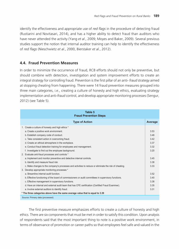
189Red Flags and Fraud Prevention on Rural Banks
identify the effectiveness and appropriate use of red flags in the procedure of detecting fraud (Rustiarini and Novitasari, 2014), and has a higher ability to detect fraud than auditors who have never attended the activity (Yang et al., 2009; Moyes and Baker, 2009). Several previous studies support the notion that internal auditor training can help to identify the effectiveness of red flags (Nieschwietz et al., 2000, Bierstaker et al., 2012).
4.4. Fraud Prevention Measures
In order to minimize the occurrence of fraud, RCB efforts should not only be preventive, but should combine with detection, investigation and system improvement efforts to create an integral strategy for controlling fraud. Prevention is the first pillar of an anti- fraud strategy aimed at stopping cheating from happening. There were 14 fraud prevention measures grouped into three main categories, i.e., creating a culture of honesty and high ethics, evaluating strategy implementation and anti-fraud control, and develop appropriate monitoring processes (Sengur, 2012) (see Table 5).
�� ��������������������������������� ������ ����
�� ����������� � ��������� ��������
�� ������ ��������������������������
�� ��������� ��������� ��� �������� ���������
�� ������������� �������������� ���������������
�� �������������������� ������ � �������������������������������
�� ����� ��������� ������������������������������
�� ����������� ������������������������������
�� ���������������� ��������� ������������ �� �����������������
�� ����� ���������������������� ���
�� ��������������������������������������������� � ������������������ � ���������� ����������� ���
�� ���������� ������� ��� �������������
�� ������� ��� ����������� ������� ���
�� ������ ������� �� ����������������������� �� ������������ ������ ������ ������ ���������� ����
�� ������ ������������� ������ ���������� ����
�� ������ ����������������������� ������������������������ � ��� �������� � ������������ �����
�� ����������������� �������� ���� ���������
������������������������������������������������������������������ ����������
��������������������������� �
�������������
���������� ��������������������
����
����
����
����
����
����
����
����
����
����
����
����
����
����
�������
The first preventive measure emphasizes efforts to create a culture of honesty and high ethics. There are six components that must be met in order to satisfy this condition. Upon analysis of respondents said that the most important thing to note is a positive work environment, in terms of observance of promotion or career paths so that employees feel safe and valued in the
190 Bulletin of Monetary Economics and Banking, Volume 19, Number 2, October 2016
job. Leaders should also consistently communicate the importance of compliance with this code in the company to reduce unethical behavior, and consequences should be consistent for acts of fraud committed. This condition is realized if the leadership of the company can create an ethical atmosphere in the workplace. If the leader has integrity and uphold the ethical values, the employee also would uphold the same values, and vice versa. Board of commissioners and board of directors of RCBs are also required to foster a culture and awareness of anti-fraud at all levels of the RCB organization.
All forms of ethical and unethical behavior are socialized through training. This activity aims to raise awareness and the ability of employees to identify fraud occurring, including taking appropriate action when knowing someone commits acts of fraud. Another important thing is, companies must have effective policies to minimize the possibility of employing or promoting employees who have a low level of honesty, especially for vital positions within the company.
Prevention efforts need to be implemented is to evaluate the implementation of both anti-fraud processes and control strategy. Given fraud occurs largely in the RCBs carried out by a company official, RCB need to have a reliable internal control system to detect possible fraud. Internal auditors need to monitor the internal control system, identify processes, controls, and other necessary procedures to mitigate the risks identified. A preventive and detective internal control system can run effectively if management has the ability to identify and quantify aspects of fraud risk assessment. The assessment process should consider the vulnerability of the company on fraud activity and whether it causes a material misstatement in the financial statements or material losses for the company. Other activities that may be done to reduce or eliminate the risk of fraud is making changes to processes and activities of the company. This step is necessary to reduce the chances of certain parties from studying the existing systems and preventing the use of the same type of fraud in the future.
The successful implementation of fraud prevention measures is highly dependent on policy support and some internal party decision-maker. In order to strengthen the internal control system, the RCB is required to activate the role of internal auditors or IBS. This role would function to be in charge of and responsible for (1) assisting the board of directors and board of commissioners in operational control of the RCB; (2) analysis and assessment in the areas of finance, accounting and operations, and other activities by means of direct examination and analysis of documents; (3) identify all possibilities to improve and increase the efficient use of resources and funds; and (4) provide recommendations for improvements and information on the activities examined at all levels of management. If this role is functioning properly, it can minimize the potential risks.
The role of supervision is also performed by the Board of Directors and Audit Committee. The Audit Committee helps the Board of Commissioners fulfill its oversight responsibilities in the financial reporting process and internal control systems of banking. The Board of Directors
191Red Flags and Fraud Prevention on Rural Banks
as the management of the RCB should monitor the activities of internal control because it has a responsibility to present the financial statements as reasonable. Management should follow-up on audit findings and recommendations from the working unit or official responsible for the implementation of RCB internal audit, external auditor, the results of the Supervisory Board of Directors, the FSA, and / or other authorities. Thus, management is responsible to take steps to prevent and detect fraud. To be able to apply the principles of accountability and transparency, the RCB may involve the external auditor of a public accounting firm to identify fraud. Do not rule out the leadership role of the RCB to facilitate internal auditors to follow a certification relating to the CFE (Certified Fraud Examiner). CFE certified auditors who may be part of a team of internal auditors or external auditors so as to assist the Board of Commissioners and Board of Directors in aspects of monitoring.
V. CONCLUSION
Banking fraud requires more serious attention. Not infrequently this condition ends with the liquidation of the bank, and certainly has a negative impact on the image of the RCB industry. The decline in public trust in RCBs can also be extended to other banks. Internal auditors as part of the internal control system of RCB into endeavor to reveal the occurrences of fraud. The function of internal audit must be able to ensure a healthy RCB, for it develop as it should, and to be able to provide optimum service to the community.
Results from this study suggest that the fraud indicators (red flags) can be effectively used in the detection of fraud. The dimensions of the Fraud Diamond that has the highest average value is ability (capability). This means that fraud can occur when there is a pressure, opportunity, rationalization, and the ability of perpetrators to commit fraud. Theoretically, this study complements previous research limitations that still used the concept of The Fraud Triangle.
The test results on the demographic characteristics of the internal auditor is influenced by education, years of experience in detecting fraud, as well as the relevant training, while gender and age did not affect the perception of internal auditors on the effectiveness of red
flags in detecting fraud in the banking world.
In addition to identifying the effectiveness of red flags in detecting fraud, RCBs also made attempts at fraud prevention. The efforts can be characterized in three groups, i.e., create a culture of honesty and high ethics, evaluate anti-fraud implementation and control strategy, and develop appropriate monitoring process.
So that preventive measures can be run effectively, the top leadership in management of the bank has to understand and recognize the risks in carrying out its business activities so that all aspects of the risks involved can anticipated early. It is important to understand the types of preventive factors necessary in an environment where fraud is done.

192 Bulletin of Monetary Economics and Banking, Volume 19, Number 2, October 2016
A good understanding of the various parties would be to optimize the prevention of fraud in RCB. In addition to using red flags as indicators of fraud, the RCB management should combine these indicators with other analytical methods such as predictive failure of the company, creative accounting practices, and models that can predict the behavior of employees. This is to ensure the continuity of operations at the RCB in the long term, ensuring the availability of financial services to SMEs and communities in remote areas, as well as to improve the reputation and public confidence in the RCB.
193Red Flags and Fraud Prevention on Rural Banks
REFERENCES
American Institute of Certified Public Accountant’s. (2002). Consideration of Fraud in A Financial
Statement Audit. Statement on Auditing Standards. No. 99. New York.
Association of Certified Fraud Examiners. (2010). Report to The Nation on Occupational Fraud. https://acfe.com/ documents/2010RttN.pdf, accessed in 5 October 2016.
Albrecht , S., K. Howe and M. Romney. (1986). Red-Flagging Management: a Validation. Advances in Accounting: 323-333.
Apostolou B, Hassell J, Webber S, and Sumners G. (2001). The Relative Importance of Management Fraud Risk Factors. Behavioral Research in Accounting, 13: 1-24.
Bank Indonesia. (2016). Kajian Ekonomi dan Keuangan Regional Triwulan II 2016. http://
www.bi.go.id/id/publikasi/kajian-ekonomi-regional/bali/Pages/Kajian Ekonomi-dan-
KeuanganRegional-Provinsi-Bali-Agustus-2016.aspx accessed in 1 December 2016.
Bank Indonesia. (2016). Surat Edaran Bank Indonesia No.13/28/DPNP tentang Penerapan Strategi
Anti Fraud bagi Bank Umum.
Bierstaker, J.L., J. E. Huntn, and J. C Thibodeau. (2012). Does Fraud Training Help Auditors Identify Fraud Risk Factors? Advances in Accounting Behavioral Research, 15: 85–100.
Blokdijk H., Drieenhuizen F, Simunic DA, and Stein MT. (2003). Factors Affecting Auditors’ Assessments of Planning Materiality. Auditing: A Journal of Practice & Theory, 22 (2): 297–307.
Choo, F. and Tan, K. (2007). An “American Dream” Theory of Corporate Executive Fraud. Accounting Forum, 31 (2): 203-215.
oram P, Ferguson C, and Moroney R. (2008). Internal Audit, Alternative Internal Audit Structures and the Level of Misappropriation of Assets Fraud. Accounting & Finance, 4: 543–59.
Cressey, D. R. (1950). The Criminal Violation of Financial Trust. American Sociological Review, 15 (6): 738–743.
Cressey, D. R. (1953). Other People’s Money; A Study of the Social Psychology of Embezzlement. New York, NY: Free Press.
Friedman, S. (1995). Case Study: Pay Attention to Warning Signals. Journal of Accountancy: 65-80.
Ghozali, Imam. (2011). Aplikasi Analisis Multivariate Dengan Program IBM. SPSS 19 (Fifth Edition) Semarang: Universitas Diponegoro.
194 Bulletin of Monetary Economics and Banking, Volume 19, Number 2, October 2016
Gillentine, A. (2009). Business Fraud on the Rise During Recession. The Colorado Springs Business Journal. http://csbj.com/2009/12/17/business-fraud-on-the-rise-during-recession accessed in 5 October 2016.
Gulllkvist, B and A. Jokippi. (2013). Perceived Importance of Red Flags Across Fraud Types. Critical Perspectives on Accounting, 24: 44–61.
Groveman, H. (1995). How Auditors can Detect Financial Statements Misstatement. Journal
of Accountancy: 83-86.
Hay, L. (2013). The Changing Profile of Fraud. http://www.ohioscpa.com/mobile/current-
news/2013/03/13/the-changing-profile-offraud?c=1 accessed in 5 October 2016
Hegazy, Mohamed and Kassem, Rasha. (2010). Fraudulent Financial Reporting: Do Red Flags Really Help? International Journal of Academic Research: Economics and
Engineering, 4: 69 – 79.
Heiman-Hoffman, Vicky B, Kimberly P. Morgan and James M Patton, (1996). The Warning Signs of Fraudulent Financial Reporting. Journal of Accountancy, 182 (4).
Kaplan, S. and Reckers, P. M. J. (1995). Auditors’ Reporting Decisions for Accounting Estimates: The Effect of Assessments of The Risk of Fraudulent Financial Reporting, Managerial
Auditing Journal, 10 (5): 27-36.
KPMG. (2009). Fraud Survey 2009. http://www.kpmg.com/ZA/en/IssuesandInsights/
ArticlesPublications/Risk-Compliance/Pages/Fraud-Survey-2009.aspx. Accessed in 5 October 2016.
Koornhof, C. and Plessis, D Du. (2000). Red Flagging as an Indicator of Financial Statement Fraud: The Perspective of Investors and Lenders. Meditari Accountancy
Research, 8: 69-93.
Libby, R. and D.M. Frederick. (1990). Experience and the Ability to Explain Audit Findings. Journal of Accounting Research, 28 (2): 348-367.
Liou F-M. (2008). Fraudulent Financial Reporting Detection and Business Failure Prediction Models: A Comparison. Managerial Auditing Journal, 7: 650–62.
Messier Jr WF, Martinov-Bennie N, and Eilifsen A. A (2005). Review and Investigation of Empirical Research on Materiality: Two Decades Later. Auditing: A Journal of
Practice & Theory, 2:153–87.
Moeller. (2009). Brink’s Modern Internal Auditing, 7th Edition. New Jersey: John Wiley & Sons.
Moyes, Glen D., Ping Lin, Raymond M. Landry, and Handan Vicdan. (2006). Red Flags Detecting Fraud. Journal of Accounting, Ethics & Public Policy, 6 (1): 1-28.
195Red Flags and Fraud Prevention on Rural Banks
Moyes, Glen D. (2007). The Differences in Perceived Level of Fraud-Detecting Effectiveness of SAS No. 99 Red Flags Between External and Auditor Internals. Journal of Business &
Economics Research. 6: 9-25.
Moyes, G.D. and C. R. Baker. (2009). Factors Influencing The Use of Red Flags to Detect Fraudulent Financial Reporting, Internal Auditing, 24 (3): 33-40.
Moyes, Glen D., Mohamed Din, and Hesri Faizal. (2013). Malaysian Internal and External Auditor Perceptions of the Effectiveness of Red Flags for Detecting Fraud. International Journal of Auditing Technology, 1 (1): 91-106.
Nieschwietz, R. J., Schultz, J. J., and Zimbelman, M. F. (2000). Empirical Research on External Auditors’ Detection of Financial Statement Fraud. Journal of Accounting Literature, 19: 190-246.
Norman C, Rose J, and Suh I. (2011) The Effects of Disclosure Type and Audit Committee Expertise on Chief Audit Executives’ Tolerance for Financial Misstatements. Accounting, Organizations and Society, 36:102–8.
Omar, Normah Binti. (2011). Fraud Diamond Risk Indicator: an Assessment of Its Importance and Usage. http://www.researhgate.net/publication accessed in 5 October 2016.
Omar, Normah Binti Omar, and H. F. Mohamad Din. (2010). Fraud Diamond Risk Indicator: An Assessment of Its Importance and Usage. http://ieeexplore.ieee.org/ document/5773853/ accessed in 5 October 2016.
Otoritas Jasa Keuangan. (2015). Peraturan Otoritas Jasa Keuangan No 4/POJK.03/2015 tentang Penerapan Tata Kelola bagi Bank Perkreditan Rakyat.
Otoritas Jasa Keuangan. (2016). Surat Edaran Otoritas Jasa Keuangan No 7/SEOJK.03/2016
tentang Standar Pelaksanaan Fungsi Audit Intern Bank Perkreditan Rakyat.
Otoritas Jasa Keuangan. (2016). Laporan Profil Industri Perbankan Triwulan I-2016.
Pincus, Karen V. (1989). The Efficacy of A Red Flags Questionnaire for Assessing The Possibility of Fraud. Accounting, Organizations and Society, 12 (1-2): 153-163.
PriceWater House Coopers. (2009). The Global Economic Crime Survey: Economic Crime in A
Downturn
PriceWater House Coopers (2004). The Emerging Role of Internal Audit in Mitigating Fraud
and Reputation Risk.
Radar Bali Jawa Pos. (2016). Kondisi Tak Pasti, Kecurangan Belum Berhenti. 27th Edition November 2016, page 21.
Robbins, Stephen A., and Judge, Timothy. (2008). Perilaku Organisasi 2. 12th Edition. Jakarta: Salemba Empat.
196 Bulletin of Monetary Economics and Banking, Volume 19, Number 2, October 2016
Rustiarini, Ni Wayan and Ni Luh Gde Novitasari. (2014). Persepsi Auditor atas Efektivitas Red Flags untuk Mendeteksi Kecurangan Pelaporan Keuangan. Journal of Accounting
Multiparadigma, 05 (3): 345-354.
Rustendi, T. (2009). Analisis terhadap Faktor Pemicu Terjadinya Fraud (Suatu Kajian Teoritis bagi Kepentingan Audit Internal). Journal of Accounting, 9 (2): 705-714.
Sengur, Evren Dilek. (2012). Auditors’ Perception of Fraud Prevention Measures: Evidence from Turkey. Annales Universitatis Apulensis Series Oeconomica, 14 (1): 128-138.
Tuanakotta, Theodorus M. (2010). Akuntansi Forensik dan Audit Investigatif. 2nd Edition. Jakarta: Salemba Empat.
Wolfe, David T. and D. R. Hermanson. (2004). The Fraud Diamond: Considering The Four Elements of Fraud. The Certified Public Accountants (CPA) Journal. December: 38-42.
Weisenborn, D. and Norris, D.M. (1997). Red Flags of Management Fraud, National Public Accountant, 42 (2): 29-33.
Yang, Weifang, Moyes, Glen D., Hamedian, Hamed, and Rahradian, Azar. (2010). P ro fess iona l Demograph ic Fac tor s That In f luence I ran ian Aud i to r s ’ Perceptions of the Fraud-Detecting Effectiveness of Red Flags. International Business &
Economics Research Journal, 9 (1): 83-102.
Yulifah, Anna and Gugus Irianto. (2014). Persepsi Auditor Eksternal tentang Determinan Pencegahan Kecurangan Laporan Keuangan. Jurnal Ilmiah Mahasiswa FEB Universitas Brawijaya, 2 (2) http://portalgaruda.org accessed in 5 October 2016.
http://beritadewata.com/Ekonomi-dan-Bisnis/Badung/OJK-Gelar-Diskusi-Ditengah-Ketatnya-
Persaingan-BPR.html accessed in 17 November 2016
http://bali.bisnis.com/read/20151215/14/56043/kinerja-bpr-di-bali-kredit-tumbuh-125 accessed in 17 November 2016
http://bisniskeuangan.kompas.com/read/2016/06/09/204422226/tahun.2005.sampai.2016.
lps.likuidasi.71.bank accessed in 22 September 2016.
http://bali.tribunnews.com/2016/05/11/kredit-macet-bpr-di-bali-capai-427-persen-ini-saran-ojk accessed in 17 November 2016
http://finansial.bisnis.com/read/20110513/90/30259/hampir-70-percent-bpr-tutup-karena-fraud
accessed in 22 September 2016.
https://finance.detik.com/moneter/d-3344651/bpr-paling-banyak-lakukan-pidana perbankan-
ini-sebabnya accessed in 17 November 2016
http://infobanknews.com/bpr-ditutup-lagi-lagi-karena-fraud/ accessed in 22 September 2016.
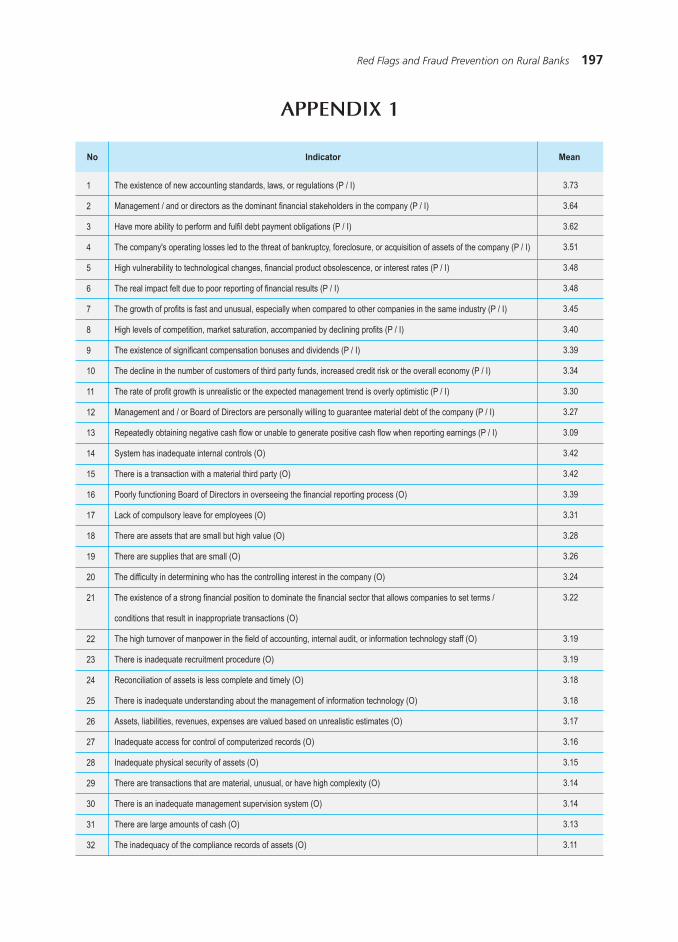
197Red Flags and Fraud Prevention on Rural Banks
APPENDIx 1
1
2
3
4
5
6
7
8
9
10
11
12
13
14
15
16
17
18
19
20
21
22
23
24
25
26
27
28
29
30
31
32
33
34
35
36
37
38
39
40
41
42
43
44
45
46
47
48
49
50
51
52
53
54
55
56
57
58
59
60
The existence of new accounting standards, laws, or regulations (P / I)
Management / and or directors as the dominant financial stakeholders in the company (P / I)
Have more ability to perform and fulfil debt payment obligations (P / I)
The company's operating losses led to the threat of bankruptcy, foreclosure, or acquisition of assets of the company (P / I)
High vulnerability to technological changes, financial product obsolescence, or interest rates (P / I)
The real impact felt due to poor reporting of financial results (P / I)
The growth of profits is fast and unusual, especially when compared to other companies in the same industry (P / I)
High levels of competition, market saturation, accompanied by declining profits (P / I)
The existence of significant compensation bonuses and dividends (P / I)
The decline in the number of customers of third party funds, increased credit risk or the overall economy (P / I)
The rate of profit growth is unrealistic or the expected management trend is overly optimistic (P / I)
Management and / or Board of Directors are personally willing to guarantee material debt of the company (P / I)
Repeatedly obtaining negative cash flow or unable to generate positive cash flow when reporting earnings (P / I)
System has inadequate internal controls (O)
There is a transaction with a material third party (O)
Poorly functioning Board of Directors in overseeing the financial reporting process (O)
Lack of compulsory leave for employees (O)
There are assets that are small but high value (O)
There are supplies that are small (O)
The difficulty in determining who has the controlling interest in the company (O)
The existence of a strong financial position to dominate the financial sector that allows companies to set terms /
conditions that result in inappropriate transactions (O)
The high turnover of manpower in the field of accounting, internal audit, or information technology staff (O)
There is inadequate recruitment procedure (O)
Reconciliation of assets is less complete and timely (O)
There is inadequate understanding about the management of information technology (O)
Assets, liabilities, revenues, expenses are valued based on unrealistic estimates (O)
Inadequate access for control of computerized records (O)
Inadequate physical security of assets (O)
There are transactions that are material, unusual, or have high complexity (O)
There is an inadequate management supervision system (O)
There are large amounts of cash (O)
The inadequacy of the compliance records of assets (O)
The inadequacy of the division of tasks and independent audit procedures (O)
The inadequacy of the system of authorization and approval of transactions (O)
High turnover of board of directors (O)
The organizational structure is too cumbersome (O)
There is no adequate accounting and information system (O)
Transactions are not recorded in a timely and not well documented (O)
There are portable assets (gold, computer chips) (O)
Management is dominated by a single person or a small group within the company without clear control (O)
Excessive management's desire to maintain or increase its profit (R)
Failure of management to improve timely reporting conditions (R)
Excessive participation in the selection of management accounting principles or the basis for determining the estimate (R)
Changes in behavior or lifestyle of management (R)
Management behavior dominates in dealing with the auditor (R)
Management commitment to a third party to achieve unrealistic estimation (R)
Management conducts formal or informal restrictions on the auditor (R)
Management shows the behavior of displeasure or dissatisfaction with the performance of the company (R)
Frequent disputes with previous external auditors related to accounting, auditing or financial reporting issue (R)
Management seeks to justify the difference or use of inappropriate accounting standards for the basis of materiality (R)
Management ignores the need for monitoring or reducing risks (R)
Has a history of violations of the law or engaged in fraud or irregularities, (R)
Management places unreasonable demands on the auditors to complete the audit or issue the auditor's
report in a short time (R)
Management ignores internal control over the misappropriation of assets (R)
Management uses unlawful means to minimize reported earnings by reason of reducing tax payments (R)
Someone has an important position in the organization or function (C)
Someone has the ability to understand and exploit the weaknesses of the internal control systems (C)
Someone with a very persuasive personality (capable of influencing) (C)
Someone with a strong ego and a big confidence (C)
A fraud can be said to be successful if it is effectively able to avoid detection (C)
3.73
3.64
3.62
3.51
3.48
3.48
3.45
3.40
3.39
3.34
3.30
3.27
3.09
3.42
3.42
3.39
3.31
3.28
3.26
3.24
3.22
3.19
3.19
3.18
3.18
3.17
3.16
3.15
3.14
3.14
3.13
3.11
3.10
3.09
3.07
3.05
3.05
3.05
3.03
2.97
3.46
3.35
3.27
3.27
3.26
3.25
3.14
3.12
3.07
3.03
3.02
3.01
3.00
3.00
2.99
3.85
3.74
3.47
3.42
3.38
No Indicator Mean
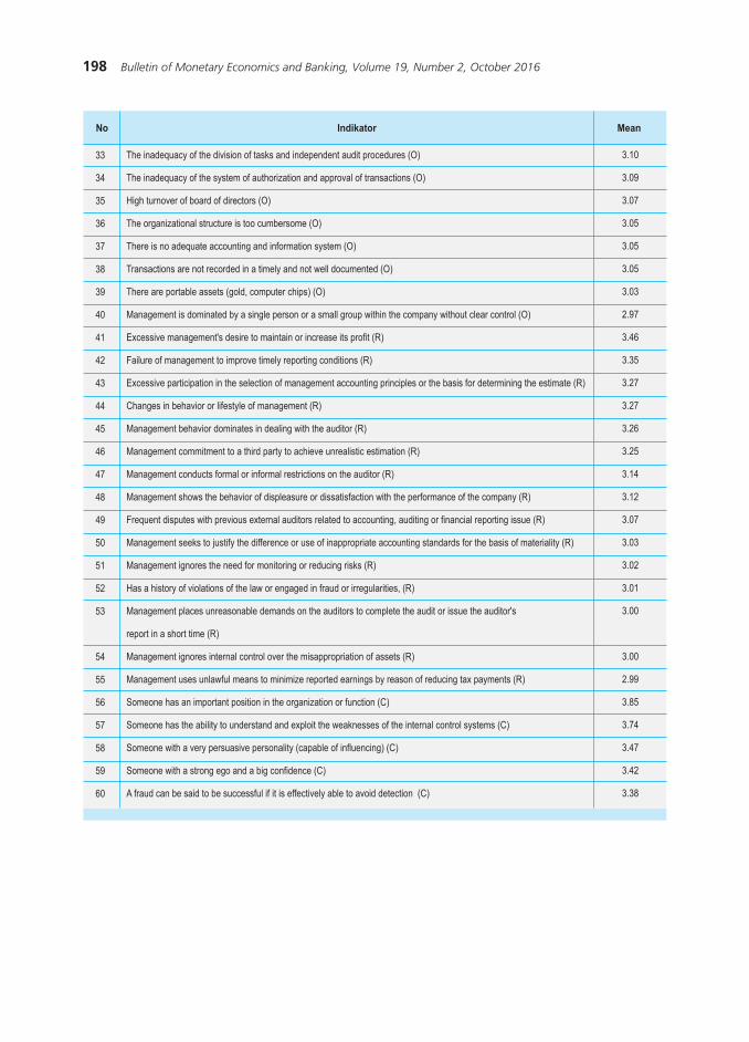
198 Bulletin of Monetary Economics and Banking, Volume 19, Number 2, October 2016
1
2
3
4
5
6
7
8
9
10
11
12
13
14
15
16
17
18
19
20
21
22
23
24
25
26
27
28
29
30
31
32
33
34
35
36
37
38
39
40
41
42
43
44
45
46
47
48
49
50
51
52
53
54
55
56
57
58
59
60
Adanya standar akuntansi, undang-undang, atau peraturan baru (P/I)
Manajemen/dan atau direksi sebagai pemangku kepentingan keuangan yang dominan dalam perusahaan (P/I)
Memiliki kemampuan lebih untuk melakukan kewajiban pemenuhan pembayaran utang (P/I)
Kerugian operasi perusahaan menyebabkan ancaman kebangkrutan, penyitaan, atau pengambilalihan aset
perusahaan (P/I)
Kerentanan tinggi terhadap perubahan teknologi, keusangan produk keuangan, atau tingkat bunga (P/I)
Dampak nyata yang dirasakan akibat pelaporan hasil keuangan yang buruk (P/I)
Pertumbuhan laba cepat dan tidak biasa, terutama bila dibandingkan dengan perusahaan lain dalam industri
yang sama (P/I)
Tingkat kompetisi tinggi, adanya kejenuhan pasar, disertai dengan penurunan laba (P/I)
Adanya bagian signifikan dari kompensasi bonus dan dividen (P/I)
Penurunan jumlah nasabah dana pihak ketiga, meningkatnya risiko kredit atau perekonomian secara
keseluruhan (P/I)
Tingkat pertumbuhan laba tidak realistis atau tren ekspektasi manajemen yang disampaikan terlalu optimis (P/I)
Manajemen dan/atau dewan direksi secara pribadi bersedia menjamin hutang perusahaan yang material (P/I)
Berulang kali memperoleh arus kas negatif atau tidak mampu menghasilkan arus kas positif ketika
melaporkan laba (P/I)
Sistem pengendalian internal tidak memadai (O)
Terdapat transaksi dengan pihak ketiga yang material (O)
Dewan direksi kurang berfungsi dalam mengawasi proses pelaporan keuangan (O)
Kurangnya cuti wajib bagi karyawan (O)
Terdapat aktiva yang berukuran kecil tetapi bernilai tinggi (O)
Terdapat persediaan yang berukuran kecil (O)
Kesulitan menentukan individu yang memiliki hak pengendalian dalam perusahaan (O)
Adanya posisi keuangan yang kuat untuk mendominasi sektor keuangan yang memungkinkan perusahaan
mengatur syarat/ ketentuan sehingga mengakibatkan transaksi yang tidak pantas (O)
Tingginya perputaran tenaga kerja bidang akuntansi, internal audit, atau staf teknologi informasi (O)
Tidak memadainya prosedur perekrutan tenaga kerja (O)
Rekonsiliasi aset kurang lengkap dan tepat waktu (O)
Tidak memadainya pemahaman manajemen tentang teknologi informasi (O)
Aset, kewajiban, pendapatan, beban dinilai berdasarkan estimasi yang tidak realistis (O)
Tidak memadainya akses pengendalian atas catatan terkomputerisasi (O)
Tidak memadainya keamanan fisik atas aset (O)
Terdapat transaksi yang material, tidak biasa, atau memiliki kompleksitas tinggi (O)
Tidak memadainya sistem pengawasan manajemen (O)
Tersedia kas dalam jumlah besar (O)
Tidak memadainya kepatuhan pencatatan atas aset (O)
Tidak memadainya pembagian tugas dan prosedur pemeriksaan yang independen (O)
Tidak memadainya sistem otorisasi dan persetujuan transaksi (O)
Tingginya pergantian dewan direksi (O)
Struktur organisasi terlalu rumit (O)
Tidak terdapat sistem akuntansi dan informasi yang memadai (O)
Transaksi tidak dicatat tepat waktu dan tidak terdokumentasi dengan baik (O)
Terdapat aset yang mudah dibawa (emas, chip komputer) (O)
Manajemen didominasi oleh satu orang atau satu kelompok kecil dalam perusahaan tanpa kontrol yang jelas (O)
Keinginan manajemen yang berlebihan untuk mempertahankan atau meningkatkan laba perusahaan (R)
Kegagalan manajemen untuk memperbaiki kondisi pelaporan secara tepat waktu (R)
Partisipasi berlebihan manajemen dalam pemilihan prinsip akuntansi atau dasar penentuan estimasi (R)
Perubahan perilaku atau gaya hidup manajemen (R)
Perilaku manajemen mendominasi dalam berurusan dengan auditor (R)
Komitmen manajemen kepada pihak ketiga untuk mencapai estimasi yang tidak realistis (R)
Manajemen melakukan pembatasan formal atau informal pada auditor (R)
Manajemen menunjukkan perilaku ketidaksenangan atau ketidakpuasan atas kinerja perusahaan (R)
Sering terjadi perselisihan dengan auditor eksternal terdahulu terkait dengan akuntansi, audit, atau masalah
pelaporan keuangan (R)
Manajemen berupaya membenarkan selisih atau menggunakan standar akuntansi yang tidak pantas untuk
dasar materialitas (R)
Manajemen mengabaikan kebutuhan untuk memantau atau mengurangi risiko (R)
Memiliki sejarah pelanggaran hukum atau terlibat dalam kecurangan atau pelanggaran hukum (R)
Manajemen memberikan tuntutan tidak masuk akal pada auditor untuk menyelesaikan audit atau menerbitkan
laporan auditor dalam waktu yang singkat (R)
Manajemen mengabaikan pengendalian internal atas penyalahgunaan aset (R)
Manajemen menggunakan cara tidak legal untuk meminimalkan laba yang dilaporkan dengan alasan
mengurangi pembayaran pajak (R)
Seseorang memiliki posisi atau fungsi penting dalam organisasi (C)
Seseorang memiliki kemampuan untuk memahami dan mengeksploitasi kelemahan pengendalian internal (C)
Seseorang dengan kepribadian yang sangat persuasif (mampu mempengaruhi) (C)
Seseorang memiliki ego yang kuat dan keyakinan besar (C)
Suatu kecurangan dapat dikatakan berhasil apabila secara efektif mampu menghindari pendeteksian
kecurangan (C)
3,73
3,64
3,62
3,51
3,48
3,48
3,45
3,40
3,39
3,34
3,30
3,27
3,09
3,42
3,42
3,39
3,31
3,28
3,26
3,24
3,22
3,19
3,19
3,18
3,18
3,17
3,16
3,15
3,14
3,14
3,13
3,11
3,10
3,09
3,07
3,05
3,05
3,05
3,03
2,97
3,46
3,35
3,27
3,27
3,26
3,25
3,14
3,12
3,07
3,03
3,02
3,01
3,00
3,00
2,99
3,85
3,74
3,47
3,42
3,38
No Indikator Mean
1
2
3
4
5
6
7
8
9
10
11
12
13
14
15
16
17
18
19
20
21
22
23
24
25
26
27
28
29
30
31
32
33
34
35
36
37
38
39
40
41
42
43
44
45
46
47
48
49
50
51
52
53
54
55
56
57
58
59
60
The existence of new accounting standards, laws, or regulations (P / I)
Management / and or directors as the dominant financial stakeholders in the company (P / I)
Have more ability to perform and fulfil debt payment obligations (P / I)
The company's operating losses led to the threat of bankruptcy, foreclosure, or acquisition of assets of the company (P / I)
High vulnerability to technological changes, financial product obsolescence, or interest rates (P / I)
The real impact felt due to poor reporting of financial results (P / I)
The growth of profits is fast and unusual, especially when compared to other companies in the same industry (P / I)
High levels of competition, market saturation, accompanied by declining profits (P / I)
The existence of significant compensation bonuses and dividends (P / I)
The decline in the number of customers of third party funds, increased credit risk or the overall economy (P / I)
The rate of profit growth is unrealistic or the expected management trend is overly optimistic (P / I)
Management and / or Board of Directors are personally willing to guarantee material debt of the company (P / I)
Repeatedly obtaining negative cash flow or unable to generate positive cash flow when reporting earnings (P / I)
System has inadequate internal controls (O)
There is a transaction with a material third party (O)
Poorly functioning Board of Directors in overseeing the financial reporting process (O)
Lack of compulsory leave for employees (O)
There are assets that are small but high value (O)
There are supplies that are small (O)
The difficulty in determining who has the controlling interest in the company (O)
The existence of a strong financial position to dominate the financial sector that allows companies to set terms /
conditions that result in inappropriate transactions (O)
The high turnover of manpower in the field of accounting, internal audit, or information technology staff (O)
There is inadequate recruitment procedure (O)
Reconciliation of assets is less complete and timely (O)
There is inadequate understanding about the management of information technology (O)
Assets, liabilities, revenues, expenses are valued based on unrealistic estimates (O)
Inadequate access for control of computerized records (O)
Inadequate physical security of assets (O)
There are transactions that are material, unusual, or have high complexity (O)
There is an inadequate management supervision system (O)
There are large amounts of cash (O)
The inadequacy of the compliance records of assets (O)
The inadequacy of the division of tasks and independent audit procedures (O)
The inadequacy of the system of authorization and approval of transactions (O)
High turnover of board of directors (O)
The organizational structure is too cumbersome (O)
There is no adequate accounting and information system (O)
Transactions are not recorded in a timely and not well documented (O)
There are portable assets (gold, computer chips) (O)
Management is dominated by a single person or a small group within the company without clear control (O)
Excessive management's desire to maintain or increase its profit (R)
Failure of management to improve timely reporting conditions (R)
Excessive participation in the selection of management accounting principles or the basis for determining the estimate (R)
Changes in behavior or lifestyle of management (R)
Management behavior dominates in dealing with the auditor (R)
Management commitment to a third party to achieve unrealistic estimation (R)
Management conducts formal or informal restrictions on the auditor (R)
Management shows the behavior of displeasure or dissatisfaction with the performance of the company (R)
Frequent disputes with previous external auditors related to accounting, auditing or financial reporting issue (R)
Management seeks to justify the difference or use of inappropriate accounting standards for the basis of materiality (R)
Management ignores the need for monitoring or reducing risks (R)
Has a history of violations of the law or engaged in fraud or irregularities, (R)
Management places unreasonable demands on the auditors to complete the audit or issue the auditor's
report in a short time (R)
Management ignores internal control over the misappropriation of assets (R)
Management uses unlawful means to minimize reported earnings by reason of reducing tax payments (R)
Someone has an important position in the organization or function (C)
Someone has the ability to understand and exploit the weaknesses of the internal control systems (C)
Someone with a very persuasive personality (capable of influencing) (C)
Someone with a strong ego and a big confidence (C)
A fraud can be said to be successful if it is effectively able to avoid detection (C)
3.73
3.64
3.62
3.51
3.48
3.48
3.45
3.40
3.39
3.34
3.30
3.27
3.09
3.42
3.42
3.39
3.31
3.28
3.26
3.24
3.22
3.19
3.19
3.18
3.18
3.17
3.16
3.15
3.14
3.14
3.13
3.11
3.10
3.09
3.07
3.05
3.05
3.05
3.03
2.97
3.46
3.35
3.27
3.27
3.26
3.25
3.14
3.12
3.07
3.03
3.02
3.01
3.00
3.00
2.99
3.85
3.74
3.47
3.42
3.38
No Indicator Mean
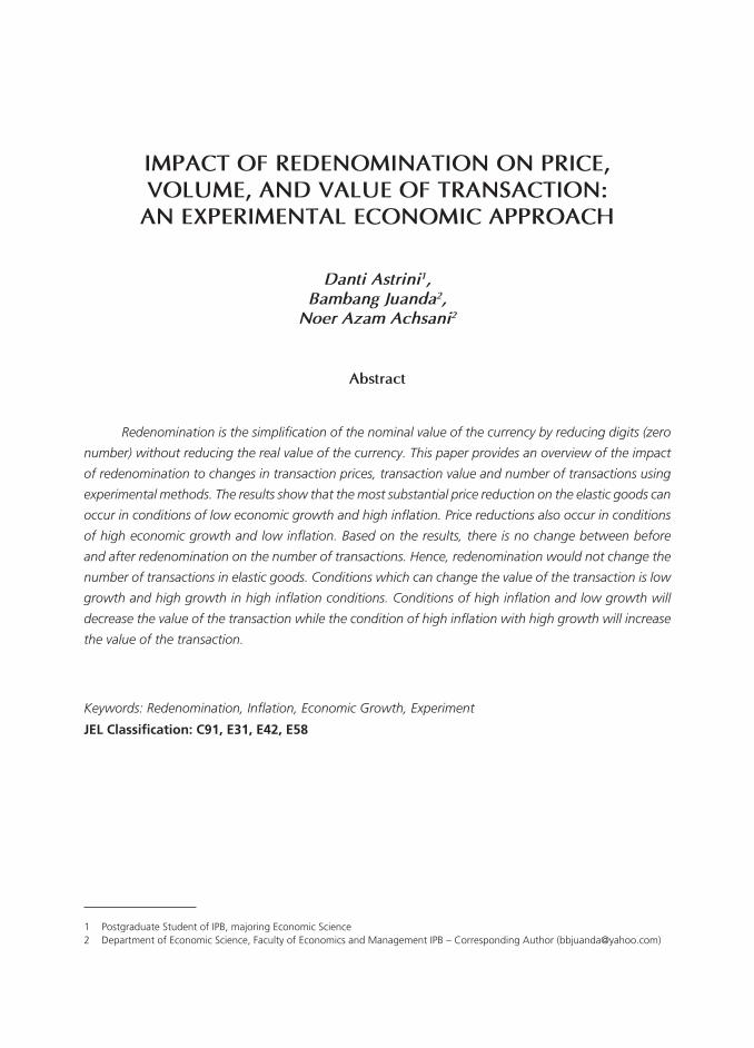
199Impact of Redenomination on Price, Volume, and Value of Transaction:
An Experimental Economic Approach
IMPACT OF REDENOMINATION ON PRICE,VOLUME, AND VALUE OF TRANSACTION: AN EXPERIMENTAL ECONOMIC APPROACH
Danti Astrini1,Bambang Juanda2,
Noer Azam Achsani2
Redenomination is the simplification of the nominal value of the currency by reducing digits (zero
number) without reducing the real value of the currency. This paper provides an overview of the impact
of redenomination to changes in transaction prices, transaction value and number of transactions using
experimental methods. The results show that the most substantial price reduction on the elastic goods can
occur in conditions of low economic growth and high inflation. Price reductions also occur in conditions
of high economic growth and low inflation. Based on the results, there is no change between before
and after redenomination on the number of transactions. Hence, redenomination would not change the
number of transactions in elastic goods. Conditions which can change the value of the transaction is low
growth and high growth in high inflation conditions. Conditions of high inflation and low growth will
decrease the value of the transaction while the condition of high inflation with high growth will increase
the value of the transaction.
Abstract
Keywords: Redenomination, Inflation, Economic Growth, Experiment
JEL Classification: C91, E31, E42, E58
1 Postgraduate Student of IPB, majoring Economic Science2 Department of Economic Science, Faculty of Economics and Management IPB – Corresponding Author ([email protected])
200 Bulletin of Monetary Economics and Banking, Volume 19, Number 2, October 2016
I. INTRODUCTION
Bank Indonesia plans to do redenomination of its currency has generated a lot of pros and cons among economic actors. Rupiah redenomination is a simplification of the number of digits on the denomination or fractional amount without reducing rupiah purchasing power, price and against the price of goods and / or services. Redenomination is different from Sanering, but there are still many Indonesian people who misunderstand the difference between the two terms. Sanering is a cut against the value of money, but the price of the goods does not change. The rationale for this redenomination of Rupiah currency is in order to face the challenges ahead in the form of regional economic integration3.
Another reason for the Rupiah to be simplified is that Indonesia’s relatively high economic growth will increase the velocity of money with increasing value. This increase affects the recording of more and more digits in every transaction that occurs, making it difficult for some parties in their financial records. The more digits in the currency, the higher the technical constraints in cash and non-cash payment transactions. Compared to other currencies, the Rupiah is included into 10 garbage money or has the third highest exchange rate against the US Dollar (US $) in the world, this can be seen in Table 1.
A too big nominal value seems to reflect in the past of a country that experienced a high rate of inflation or experienced a fundamental condition of a poor economy (Kesumajaya, 2011). If a country experiences such a thing, then the public will be less confident to hold the domestic currency and there would low credibility of both government fiscal and monetary policies. Aside from being a means of payment, the currency is also believed to be one of the symbols of the sovereignty of a nation and state. Therefore, currencies need to be respected nationally and internationally. Currently the highest denominations of the Rupiah is Rp100,000, which is the second highest currency denomination after the Vietnamese 500,000 Dong. If Indonesia continues to experience high inflation every year then it is estimated it will need a denominations of Rp200,000 even Rp1,000,000. If it happens, then the value of money on goods will be lower (Amir, 2011).
3 Press Release of Bank Indonesia No. 12/38 / PSHM / PR
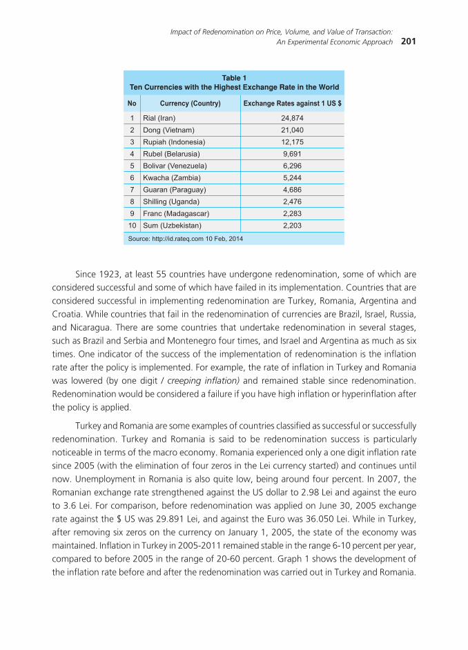
201Impact of Redenomination on Price, Volume, and Value of Transaction:
An Experimental Economic Approach
Since 1923, at least 55 countries have undergone redenomination, some of which are considered successful and some of which have failed in its implementation. Countries that are considered successful in implementing redenomination are Turkey, Romania, Argentina and Croatia. While countries that fail in the redenomination of currencies are Brazil, Israel, Russia, and Nicaragua. There are some countries that undertake redenomination in several stages, such as Brazil and Serbia and Montenegro four times, and Israel and Argentina as much as six times. One indicator of the success of the implementation of redenomination is the inflation rate after the policy is implemented. For example, the rate of inflation in Turkey and Romania was lowered (by one digit / creeping inflation) and remained stable since redenomination. Redenomination would be considered a failure if you have high inflation or hyperinflation after the policy is applied.
Turkey and Romania are some examples of countries classified as successful or successfully redenomination. Turkey and Romania is said to be redenomination success is particularly noticeable in terms of the macro economy. Romania experienced only a one digit inflation rate since 2005 (with the elimination of four zeros in the Lei currency started) and continues until now. Unemployment in Romania is also quite low, being around four percent. In 2007, the Romanian exchange rate strengthened against the US dollar to 2.98 Lei and against the euro to 3.6 Lei. For comparison, before redenomination was applied on June 30, 2005 exchange rate against the $ US was 29.891 Lei, and against the Euro was 36.050 Lei. While in Turkey, after removing six zeros on the currency on January 1, 2005, the state of the economy was maintained. Inflation in Turkey in 2005-2011 remained stable in the range 6-10 percent per year, compared to before 2005 in the range of 20-60 percent. Graph 1 shows the development of the inflation rate before and after the redenomination was carried out in Turkey and Romania.
��
�
�
�
�
�
�
�
�
�
��
��������� �
� ������ ���
��������� � �����
�����������������
���������� �������
� ������������
����� ����������
������ ���� ���
��� �����������
�������������� �
��������������������������������� ����������� �����������������
������������������ ��������� �����������������
������
������
������
�����
�����
�����
�����
�����
�����
�����
������������������������������������
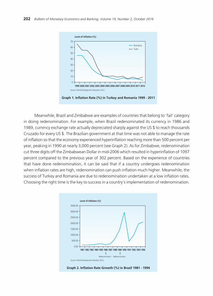
202 Bulletin of Monetary Economics and Banking, Volume 19, Number 2, October 2016
Meanwhile, Brazil and Zimbabwe are examples of countries that belong to ‘fail’ category in doing redenomination. For example, when Brazil redenominated its currency in 1986 and 1989, currency exchange rate actually depreciated sharply against the US $ to reach thousands Cruzado for every US $. The Brazilian government at that time was not able to manage the rate of inflation so that the economy experienced hyperinflation reaching more than 500 percent per year, peaking in 1990 at nearly 3,000 percent (see Graph 2). As for Zimbabwe, redenomination cut three digits off the Zimbabwean Dollar in mid-2006 which resulted in hyperinflation of 1097 percent compared to the previous year of 302 percent. Based on the experience of countries that have done redenomination, it can be said that if a country undergoes redenomination when inflation rates are high, redenomination can push inflation much higher. Meanwhile, the success of Turkey and Romania are due to redenomination undertaken at a low inflation rates. Choosing the right time is the key to success in a country’s implementation of redenomination.
Graph 1. Inflation Rate (%) in Turkey and Romania 1999 - 2011
Graph 2. Inflation Rate Growth (%) in Brazil 1981 - 1994
���� ���� ���� ���� ���� ���� ���� ���� ���� ���� ���� ���� ���� �����
��
��
��
��
��
��
��
���������� ����� ���
������������
� ����� �������� ������������ ������
����
������
�������
�������
�������
�������
�������
�������
���� ���� ���� ���� ���� ���� ���� ���� ���� ���� ���� ���� ���� ����
���������� ����� ���
�������������� ��������������
���� ���������������������� ����������
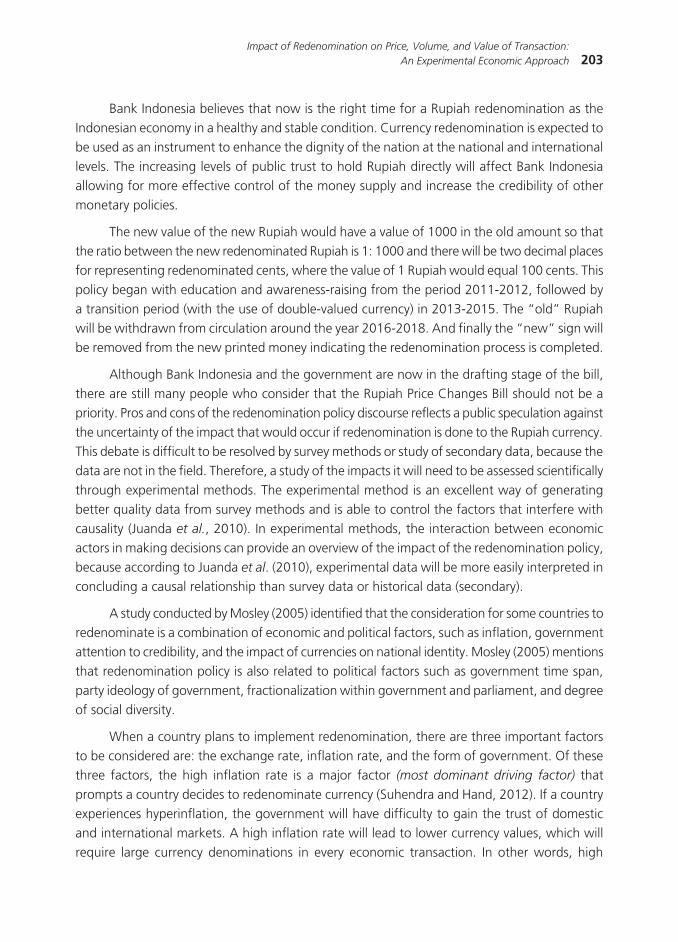
203Impact of Redenomination on Price, Volume, and Value of Transaction:
An Experimental Economic Approach
Bank Indonesia believes that now is the right time for a Rupiah redenomination as the Indonesian economy in a healthy and stable condition. Currency redenomination is expected to be used as an instrument to enhance the dignity of the nation at the national and international levels. The increasing levels of public trust to hold Rupiah directly will affect Bank Indonesia allowing for more effective control of the money supply and increase the credibility of other monetary policies.
The new value of the new Rupiah would have a value of 1000 in the old amount so that the ratio between the new redenominated Rupiah is 1: 1000 and there will be two decimal places for representing redenominated cents, where the value of 1 Rupiah would equal 100 cents. This policy began with education and awareness-raising from the period 2011-2012, followed by a transition period (with the use of double-valued currency) in 2013-2015. The “old” Rupiah will be withdrawn from circulation around the year 2016-2018. And finally the “new” sign will be removed from the new printed money indicating the redenomination process is completed.
Although Bank Indonesia and the government are now in the drafting stage of the bill, there are still many people who consider that the Rupiah Price Changes Bill should not be a priority. Pros and cons of the redenomination policy discourse reflects a public speculation against the uncertainty of the impact that would occur if redenomination is done to the Rupiah currency. This debate is difficult to be resolved by survey methods or study of secondary data, because the data are not in the field. Therefore, a study of the impacts it will need to be assessed scientifically through experimental methods. The experimental method is an excellent way of generating better quality data from survey methods and is able to control the factors that interfere with causality (Juanda et al., 2010). In experimental methods, the interaction between economic actors in making decisions can provide an overview of the impact of the redenomination policy, because according to Juanda et al. (2010), experimental data will be more easily interpreted in concluding a causal relationship than survey data or historical data (secondary).
A study conducted by Mosley (2005) identified that the consideration for some countries to redenominate is a combination of economic and political factors, such as inflation, government attention to credibility, and the impact of currencies on national identity. Mosley (2005) mentions that redenomination policy is also related to political factors such as government time span, party ideology of government, fractionalization within government and parliament, and degree of social diversity.
When a country plans to implement redenomination, there are three important factors to be considered are: the exchange rate, inflation rate, and the form of government. Of these three factors, the high inflation rate is a major factor (most dominant driving factor) that prompts a country decides to redenominate currency (Suhendra and Hand, 2012). If a country experiences hyperinflation, the government will have difficulty to gain the trust of domestic and international markets. A high inflation rate will lead to lower currency values, which will require large currency denominations in every economic transaction. In other words, high
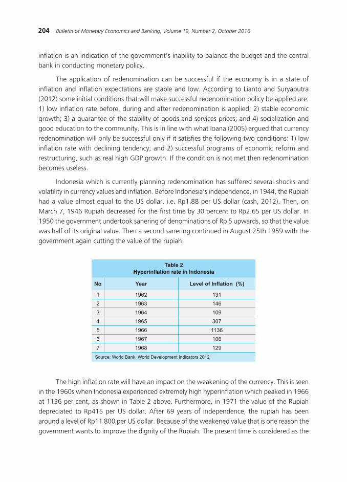
204 Bulletin of Monetary Economics and Banking, Volume 19, Number 2, October 2016
inflation is an indication of the government’s inability to balance the budget and the central bank in conducting monetary policy.
The application of redenomination can be successful if the economy is in a state of inflation and inflation expectations are stable and low. According to Lianto and Suryaputra (2012) some initial conditions that will make successful redenomination policy be applied are: 1) low inflation rate before, during and after redenomination is applied; 2) stable economic growth; 3) a guarantee of the stability of goods and services prices; and 4) socialization and good education to the community. This is in line with what Ioana (2005) argued that currency redenomination will only be successful only if it satisfies the following two conditions: 1) low inflation rate with declining tendency; and 2) successful programs of economic reform and restructuring, such as real high GDP growth. If the condition is not met then redenomination becomes useless.
Indonesia which is currently planning redenomination has suffered several shocks and volatility in currency values and inflation. Before Indonesia’s independence, in 1944, the Rupiah had a value almost equal to the US dollar, i.e. Rp1.88 per US dollar (cash, 2012). Then, on March 7, 1946 Rupiah decreased for the first time by 30 percent to Rp2.65 per US dollar. In 1950 the government undertook sanering of denominations of Rp 5 upwards, so that the value was half of its original value. Then a second sanering continued in August 25th 1959 with the government again cutting the value of the rupiah.
��
�
�
�
�
�
�
�
����
����
����
����
����
����
����
������������������������������������ ��
���� �����������������������
���
���
���
���
����
���
���
�������� ��������� �������������������������������
The high inflation rate will have an impact on the weakening of the currency. This is seen in the 1960s when Indonesia experienced extremely high hyperinflation which peaked in 1966 at 1136 per cent, as shown in Table 2 above. Furthermore, in 1971 the value of the Rupiah depreciated to Rp415 per US dollar. After 69 years of independence, the rupiah has been around a level of Rp11 800 per US dollar. Because of the weakened value that is one reason the government wants to improve the dignity of the Rupiah. The present time is considered as the
205Impact of Redenomination on Price, Volume, and Value of Transaction:
An Experimental Economic Approach
proper time for redenomination because the inflation rate in Indonesia has seen relative stability in recent years, and said to be of type of creeping inflation around one digit every year. Stable inflation reflects the stability of prices on some items that make up the consumer price level.
In addition to indicators of inflation, economic stability in a country is the policy maker’s main goal in guiding fiscal and monetary instruments. Economic stability is a prerequisite for the achievement of improvements in public welfare and certainty in providing investment guarantees in a country. Thus the stability of economic growth can boost economic activity in the form of trade in goods / services and financial transactions. Indonesia’s economic growth in recent years can be said to be stable to be around 5-6 per cent per year and with a tendency to increase.
In addition to the positive impacts of redenomination such as the increased credibility of the Rupiah as the government’s goal, there are also negative impacts that will occur if redenomination policies are applied. One is the possibility of misperception by thinking that redenomination is sanering. Sanering is the policy of eliminating the zeros in the currency, but the cut is not done on the price of goods, so the purchasing power of people decreases. An incorrect understanding of redenomination in society can cause panic that can give rise to a situation of economic turmoil.
In addition, with the redenomination there will be no increase in operational costs of companies and banks for changing information systems and technology that takes time for accounting adjustments to apply technology to adjust to the nominal simplification. Bank Indonesia will also incur huge costs to print new currency redenomination and public dissemination, besides other social impacts such public mistrust of the Rupiah (Kesumajaya, 2011).
Based on the statement by Wibowo (2013), the impact of which will arise because of changes in the nominal currency is the emergence of a psychological bias called money illusion. Most people would perceive that the price of goods become cheaper because of the removal of zeros from the currency value in the past. For example, suppose an increase in the price of goods amounting to Rp7,000, it is felt heavily by the consumer. But when after the redenomination hike lighter Rp7 perceived by the public. Whereas this an increase have the same value, consumers pay less attention to the process of re-scaling of the old nominal amount to the new nominal amount. Money Illusion will increasingly give an effect when consumers will see the real value of the goods they purchase due to changes in nominal prices simultaneously. If the price increase does not occur uniformly after the redenomination, the consumer will try to recalculate the real value of the goods they buy in the new nominal Rupiah, in process called re-learning.
Redenomination encourages greater consumption behavior. New prices are felt cheaper because of the occurrence of money illusion which increases consumers’ willingness to pay. Seeing a change of behavior in the society, manufacturers of goods will increase the price up to a limit which is still tolerated by consumers. Manufacturers as a rational individuals would consider rounding up the price of these goods. But on the other hand, redenomination can
206 Bulletin of Monetary Economics and Banking, Volume 19, Number 2, October 2016
reduce consumption because of the fear of inflation, causing people to switch to hold onto goods, especially those whose value is resistant to inflation. This can lead to a decrease in the currency exchange in the value of the Rupiah against other stronger currencies.
The scope of this study will examine the impact of redenomination policy to price changes, the number of transactions and the value of transactions. The data used will be obtained from the primary data of the results of experimental methods of economics. This includes the amount of the transactions, the transaction value and the price changes that occur in the goods - goods elasticity in this study uses car commodities. Redenomination is referred to in this research is the policy of elimination of three zeros in the value of Rupiah currency, unit price, wage units and everything owned by the nominal Rupiah.
The second part of this paper presents a study of the relevant literature on redenomination. Part three describes the data and methodology, especially on experimental techniques used in this paper. The fourth section presents the results of experiments and analysis, while the fifth section presents the conclusions.
II. THEORY
2.1. The Linkage of Redenomination to the Behavior of Economic Actors
The most frequent impact that occurs in the application of redenomination is the emergence of a psychological bias called money illusion (Wibowo, 2013). This illusion can arise because of the nominal price change of goods due to redenomination. Most people will perceive that the price of goods becomes cheaper because of the removal of the zero value of the previous currency. Hobijn, et al. (2006) also showed that there was money illusion in European countries that have made currency changes into the Euro. Euro is nominally fewer than previous currencies and perceived to be cheaper by the public. Hobijn, et al. (2006) argue that price increases after redenomination can be explained by the general model of the cost of menu prices, by incorporating company decisions when they adopt a new currency.
Consumers will then reevaluate their money strategy management to adapt to new currencies especially when new currencies are introduced, particularly when new currencies and old currencies are used together, when waiting for time to eliminate the old currency. Marques and Dehaene (2004) suggest that there are two main processes that can occur when a country
207Impact of Redenomination on Price, Volume, and Value of Transaction:
An Experimental Economic Approach
adopts a new currency: rescaling (converting all prices in the old currency to a value in a new currency at the same time) and re-learning (considering the new price of consumer goods one by one). The first process is predicted to experience a simple adjustment in the new currency, while the second process will undergo a longer and more complex adjustment.
Meanwhile Money / Euro Illusion shows a perception of prices in the new smaller denominations and lower currencies than when expressed in the form of the old currency if it has a higher nominal value. (Gamble et al.2002). This shows that individuals adjust to the new currency with a smaller nominal value, and at least, they have some difficulty in understanding the true value of goods and services. Money Illusion effects can also occur on goods that are cheap or can increase the price by a few cents. If the availability of cents is insufficient for the government, the consumer will tend to allow the price increase without requiring a return of change from the seller, called trivialization
Trivialization cases can be seen in Ghana where the inflation rate increased by five percent one year after redenomination. One of the contributing factors to the failure of redenomination in Ghana was that 70 per cent of the money in Ghana was outside the banking system. Cash transactions in Ghana were more dominant than transactions through banks. This condition was exacerbated by the government that has not been able to replace the old currency with a new currency after two years of redenomination. Mehdi and Motiee (2012) also revealed that the reduction in the nominal value of currencies will have psychological and social effects. When the currency has a low nominal value, then the public will feel the currency worth is strong.
Lianto and Suryaputra (2012) conducted a study to determine the impact of the implementation of redenomination in Indonesia based on the perspective of the people of Indonesia. From the data obtained by the method of the survey of 100 people who understand the redenomination and analyzed using Structural Equation Modeling, it shows that the biggest impact of redenomination is to enhance the credibility of Indonesia in the eyes of other countries. Other findings are Indonesian Muslims believe the redenomination will be in their favor. If redenomination is successfully implemented, the Rupiah currency will become stronger and increase people’s confidence in its currency. Table 3 represents some previous literature related to redenomination.
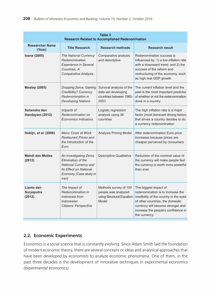
208 Bulletin of Monetary Economics and Banking, Volume 19, Number 2, October 2016
���������������������
���������� �
���������� �
��������������������������
���������������������
����������������������
������������������������
���������������������������������� ������������ ��� ��
�������������� ���������������� ���������������
��������������������������� ���������������������������������������� �����������������
������������������������������������������������ ���������������������������
� ������������� ��������������� ��������������
�����������������������������������������������������������������
������������������������� �������������������������������������������������������������� ���������������������
����� ������������ ����������������������� ������������������������������
�����������������������������������
��������������������� ���������������������������������������������
���������������������������������������������
����������������������
�����������������������
��� ����������������������������������������� ����������������������
��������������������������������������������������������������� ������������������������� ������������� ������������������������������ �������������� ��� �� ��������������
� ������������������������������� ���������� ����������������������������� �� ����������� ���������������������������������
� �� �� ���������������������������������������������������������������� ����������������������������������������������������������
���������������������������������������������������������� ���������������������������
�������������� ������������������� �������������������������������� ����������������� �������������� �������
� ������������������������������������������������� ���������������� �������������� ����������� ��������������� ��������������������������������������������������� ������������������������� �����������
2.2. Economic Experiments
Economics is a social science that is constantly evolving. Since Adam Smith laid the foundation of modern economic theory, there are several concepts or ideas and analytical approaches that have been developed by economists to analyze economic phenomena. One of them, in the past three decades is the development of innovative techniques in experimental economics (experimental economics).
209Impact of Redenomination on Price, Volume, and Value of Transaction:
An Experimental Economic Approach
In the development of experimental methods of economy, appears a theory called induced-
value theory developed by economists VL Smith in 1976 (Juanda, 2009). The basic idea of this theory is that the use of appropriate reward media allows the experimenter or researcher to elicit certain characteristics of economic actors and their innate characteristics would have no effect anymore (irrelevant). If the basic characteristics of economic actors (experimental units) are the same or homogeneous, then the researchers can experiment because the basic principle of a “controlled environment“ is maintained.
Three terms enough to bring up the above characteristics are as follows:
1. Monotonicity is the experimenter would always like the larger reward.
2. Salience is the reward received by the actor depending on their actions in the experiment according to the rules they understand.
3. Dominance: dominance of stakeholder interest in the experiment, where they prefer the reward and ignore other things.
Friedman and Sunder (1994) suggested that an economic experiment carried out in a controlled environment. The economic environment consists of economic actors along with the applicable rules or the institution as a place of interaction among economic actors. Economic actors may be buyers and sellers, and the institution may be the type of a particular market.
In economic experiments, experimental instruction consists of a description of the provisions of the experiment, the choices, and the actions that the research subject (experimenter) must perform, and the rules for awarding the reward to the subject, depending on their actions (Friedman and Sunder, 1994). The experimental instruction sheet is given to the subject of the experiment at the time the experiment will be carried out so that the subject of the study clearly understands the experimental procedure and the applicable rules. In this experimental instruction can also be equipped with a simple illustration example that will further clarify the problem for the experimental subject.
In the economic field studies with experimental methods, community groups that are often the subject of research are derived from student groups (Friedman and Sunder, 1994). Reasons for the use of students as research sources that is:
1. This group is considered the most ready to enter into the experimental group.
2. The background of this group comes from the campus, where the majority researchers appear
3. The opportunity costs is low
4. It is one way to reduce the external influences that can be a confounding variable in the study.
210 Bulletin of Monetary Economics and Banking, Volume 19, Number 2, October 2016
Economics itself only recently began to be regarded as an experimental science. This is especially true after the 1994 Nobel Prize in economics awarded to economists whose work is related to experimental economics, namely John Nash and Reinhard Selten. They provide inspiration that experimental methods can also be done in the economic field, after which the development of experimental economics grew more rapidly. Even in the wider scope (macro) some economists have tried it. Various macroeconomic or monetary policies can also be tested in the experiment.
Experimental research is interested in determining whether certain variables cause changes in behavior, thought, or emotion. In this study, researchers manipulate or change one variable (called independent variable) to see whether changes in behavior (bound variables) arise as a result. If behavioral changes arise when the independent variable is manipulated, then the researcher can conclude that the independent variable causes a change in the dependent variable (under certain conditions).
2.3. Economic Experiments in the Study of Economic Policy
In addition to testing the theories of economics, experimental economics can also be used for the assessment of economic policy. One illustration is the study conducted by Juanda et
al (2010) in reviewing and comparing the systemic effects arising from Bank Century bailout policy and the policy of closing the Bank Century by the government. The results showed that the closure of Century Bank caused a relatively low systemic impact. Significant systemic effects will be generated if bank closures are problematic in the event of a crisis in a large, troubled bank. Under normal conditions (no crisis fluctuations), the shutting down of small problem banks such as Century Bank will not have a systemic impact. Pressure and potential bank failure is very low because economic stability in normal condition is still maintained so that customer confidence in banking does not decrease.
Other research in assessing a policy with experimental method is the study of the level of tax compliance in self-assessment tax system in force in Indonesia (Juanda et al, 2010). This study examined the influence of examination opportunities, penalties and level of education on tax compliance in reporting Tax (SPT), by controlling other factors cultivated equally (ceteris
paribus). Factors that affect the level of tax compliance are difficult if using a survey design for any environmental influences or objects. The results showed that the higher probability of tax audits and greater the penalty will have positive influence on tax compliance in implementing tax obligations. Additionally, Juanda et al (2010) also stated the level of compliance to pay taxes for the “experimenter” of one strata of students was higher than the level of compliance of graduate students who have relatively high knowledge. Furthermore, the higher income taxpayer, then the lower the level of compliance.
In research to be carried out, an economic experiment is used to assess the rupiah currency redenomination policy. The procedure of the economic experiment will be done in the form of
211Impact of Redenomination on Price, Volume, and Value of Transaction:
An Experimental Economic Approach
sale and purchase transactions of consumer goods with the transaction system Posted Offer. The Posted Offer transaction system is a transaction system commonly used in the field of retail and industrial business where the price is installed by the seller then offered to the buyer (posted-offer price), and buyers then choose the desired goods in accordance with their budget.
In everyday life there are various transaction systems which include the decentralization system (DT), Double Auction (DA), and the Posted-Offer (PO). In a decentralized system, buyers and sellers freely and actively look for a partner to haggle over the price of a commodity. This transaction system is somewhat closed, because information about the seller offer (offers), the buyer’s request (bids) and the agreed price (contract price) is not recognized by all market participants or the public. While the system of double auction is a two-way paneled system, that all sellers and buyers alike haggle for a good price so that all information known to the public or all sellers and buyers in the auction (Juanda, 2009).
2.4. Experimental Simulation Procedure
The experimental simulation procedure conducted in this study is as follows:
1. Respondents who as the subject of the experimenter were first randomized with the draw to assign sellers and buyers. At low growth conditions total of respondents were numbered 10 people, divided into 5 sellers and 5 buyers. In the high growth conditions, the total respondents numbered 14 people, and further divided into 7 buyers and 7 sellers.
2. The participants were first read the experiment instructions so they would understand to their respective roles. Researchers explained detailed instructions to help the participants in experiment.
3. Participants were given a decision sheets in accordance with reviews of their respective roles. Each participant was required to record every transaction made during the experiment on the each decision sheet.
4. Buyers and sellers got the respective unit value and unit cost of each.
5. After buyers and sellers got the respective unit cost and unit value, each were then separated according to their group. Sellers, were placed be in a room, for sellers, were placed in a room, while the buyers were outside the room. Transactions were done when the buyer entered the room.
6. Prior to the transaction, the seller must specify the sale price above the unit cost given for the condition before redenomination, after which the seller directly determines the selling price for the condition after redenomination where the selling price may be fixed, more or less than the price before redenomination. The fixed price the seller has set cannot be changed when the first buyer enters the room. The market system is used in the posted
offer where there are no bargains made by the buyer in the transaction.
212 Bulletin of Monetary Economics and Banking, Volume 19, Number 2, October 2016
7. Buyers are drawn in order of purchase and then they go one by one to the seller’s room to buy goods. It continues until the last order. The first transaction is completed before the redenomination policy. After of all buying transactions are completed before redenomination, the first set of buyers re-enter the room to conduct transactions with price conditions after the redenomination policy. The buyer must buy goods at a price below the unit value.
8. Each buyer and seller must record the results of the transactions in the decision sheet.
9. Each participant performed the same procedure each time, but the initial condition (of redenomination) is determined randomly by researchers at the beginning of the month.
10. At the end of the experiment (repetition), the participants forward the decision sheets to the researchers to see the results of the profits obtained.
11. The profit gained by each test participant is calculated in accordance with the transactions attached to the experiment decision sheet.
III. RESEARCH METHODS
The type of the data that will be used in this study is primary data. The collection of primary data collection is obtained through simulations of economic experiments, where the primary data is a picture of the responses of research subjects (simulated actors) as economic actors in experiments that can be seen from decisions made by the experimental actors. The results of economic experiments were analyzed using Minitab 16 software.
3.1. Sampling Methods of Experimental Economics
Research with this economic experiment used respondents totaling 48 students from the Faculty of Economics and Management S1 IPB as the treatment subject. The sampling technique employed a multi-stage approach where the first stage uses convenience sampling to select respondents in four treatment combination involving the following groups, 10 people with low economic growth in conditions of low inflation, the 10 people with low economic growth in conditions of high inflation, 14 people with high growth in conditions of low inflation, and 14 people with high growth in conditions of high inflation.
The economic experimental method uses respondents to be rewarded according to the decisions they make. Researchers should be able streamline the use of respondents in accordance with the budget that has been made available. In this study researchers used 10 respondents for low growth and 14 respondents for high growth. The number of respondents is obtained by looking at the conditions of economic growth. Low growth is assumed by lower buying and selling activities that occur (fewer number of economic actors). While for high growth it is assumed with higher buying and selling activity that occur (large number of economic actors).
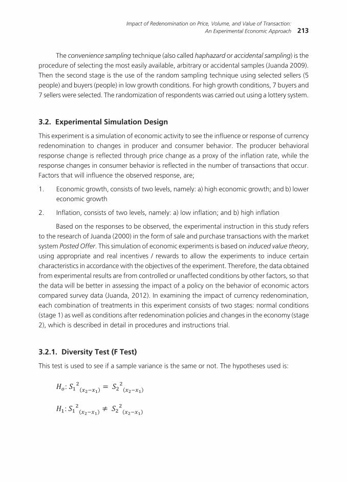
213Impact of Redenomination on Price, Volume, and Value of Transaction:
An Experimental Economic Approach
The convenience sampling technique (also called haphazard or accidental sampling) is the procedure of selecting the most easily available, arbitrary or accidental samples (Juanda 2009). Then the second stage is the use of the random sampling technique using selected sellers (5 people) and buyers (people) in low growth conditions. For high growth conditions, 7 buyers and 7 sellers were selected. The randomization of respondents was carried out using a lottery system.
3.2. Experimental Simulation Design
This experiment is a simulation of economic activity to see the influence or response of currency redenomination to changes in producer and consumer behavior. The producer behavioral response change is reflected through price change as a proxy of the inflation rate, while the response changes in consumer behavior is reflected in the number of transactions that occur. Factors that will influence the observed response, are;
1. Economic growth, consists of two levels, namely: a) high economic growth; and b) lower economic growth
2. Inflation, consists of two levels, namely: a) low inflation; and b) high inflation
Based on the responses to be observed, the experimental instruction in this study refers to the research of Juanda (2000) in the form of sale and purchase transactions with the market system Posted Offer. This simulation of economic experiments is based on induced value theory, using appropriate and real incentives / rewards to allow the experiments to induce certain characteristics in accordance with the objectives of the experiment. Therefore, the data obtained from experimental results are from controlled or unaffected conditions by other factors, so that the data will be better in assessing the impact of a policy on the behavior of economic actors compared survey data (Juanda, 2012). In examining the impact of currency redenomination, each combination of treatments in this experiment consists of two stages: normal conditions (stage 1) as well as conditions after redenomination policies and changes in the economy (stage 2), which is described in detail in procedures and instructions trial.
3.2.1. Diversity Test (F Test)
This test is used to see if a sample variance is the same or not. The hypotheses used is:

214 Bulletin of Monetary Economics and Banking, Volume 19, Number 2, October 2016
3.3. Two different tests of Population Means
Primary data generated through economic experimental design will be analyzed using the intermediate test of the middle values of two independent populations. Where the two populations in question are two different combinations of treatment groups or economic conditions. Two groups are said to be independent when the selection of the first sample units is independent of how the second sample units are selected and vice versa. Before comparing the two populations, the condition of data diversity must first be considered.
The condition of data diversity of two population can be divided into two, the same diversity (homogeneous) or σ 1
2 = σ 2 2 = σ 2 and diversity that are not the same (heterogeneous)
or σ 1 2 ≠ σ 2
2 ≠ σ 2. Both conditions will greatly determine the accuracy of the conclusions obtained. Therefore, appropriate testing methods are required for each condition. The form of hypothesis for both conditions is the same, that is:
1. H0 : μ1 – μ2 ≥ 0
H1 : μ1 – μ2 < 0 ; or
2. H0 : μ1 – μ2 ≤ 0
H1 : μ1 – μ2 > 0
Although the hypothetical form for both conditions of diversity are the same, the standard error used in the test statistic calculation is different. This can be demonstrated as follows:
If it proved to be the same variance (σ12 = σ2
2 = σ2), then the test statistic is:
(1)
where
(2)
With a degree of freedom of n1 + n2 – 2. In this case Sg is expressed as a combination of a wide variance of example 1 with a range of example 2. Whereas if the variance is not the same (σ1
2 ≠ σ22 ≠ σ2), then the test statistic is as follows:
(3)
Where 1 is the middle value of the first sample units; 2 is the middle value of the units of second instance; μ1 is the middle value the first population; μ2 is the middle value of the second population; s2
1 is the variance of the first instance; s22 is the variance of the second instance; n1
is the number of units of the first instance; an n2 is the number of units of the second instance.
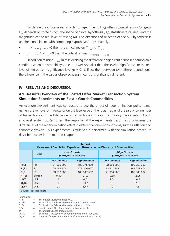
215Impact of Redenomination on Price, Volume, and Value of Transaction:
An Experimental Economic Approach
To define the critical areas in order to reject the null hypothesis (critical region to reject/ H0) depends on three things: the shape of a rival hypothesis (H1), statistical tests used, and the magnitude of the real level of testing (α). The directions of rejection of the null hypothesis is unidirectional in line with competing hypotheses items, namely:
• IfH1 : μ 1 - μ 2 <0 then the critical region T count <- T α, db
• IfH1 : μ 1 - μ 2 > 0 then the critical region T arithmetic > T α, db
In addition to using Tcount rules in deciding the difference is significant or not in a comparable condition when the probability value (p-value) is smaller than the level of significance or the real level of ten percent significance level (α = 0.1). If so, then between two different conditions, the difference in the values observed is significant or significantly different.
IV. RESULTS AND DISCUSSION
4.1. Results Overview of the Posted Offer Market Transaction System Simulation Experiments on Elastic Goods Commodities
An economic experiment was conducted to see the effect of redenomination policy items, namely the removal of three zeros on the face value of the rupiah, against the sale price, number of transactions and the total value of transactions in the car commodity market (elastic) with a buy-sell system posted offer. The response of the experimental results also compares the differences of the redenomination effect in different economic conditions, such as inflation and economic growth. This experimental simulation is performed with the simulation procedure described earlier in the method chapter.
����
���������������������������� �������� ���������� ������������������������������
�������������������������������
��������������������������������
������������� �������������� ������������� ��������������
��
�������
����������
������������
������������
�����������
���������� ��������� �
����
��
��
���� ������
�� ��������
����������������������
����
�������������������������� ������
���������
��
������������� �������������������
���������������
���������������������
Information:HKT = Theoretical Equilibrium Price (USD) P e Sb = Empirical Price Balance before the redenomination (USD) P e Sr. = Empirical Price Balance after redenomination (USD)ΔPSr = Price Changes After the redenomination (percent) JKT = Theoretical balance amount (units) Q e Sb = Empirical Transaction Amount before redenomination (units) Q e Sr. = Number of Empirical Transactions after redenomination (units)
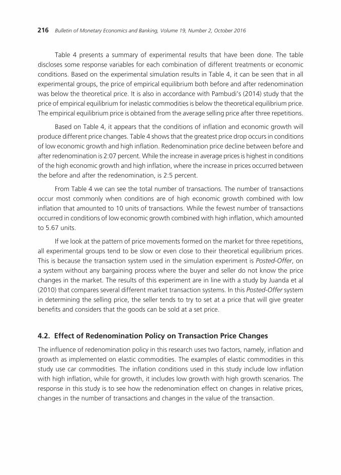
216 Bulletin of Monetary Economics and Banking, Volume 19, Number 2, October 2016
Table 4 presents a summary of experimental results that have been done. The table discloses some response variables for each combination of different treatments or economic conditions. Based on the experimental simulation results in Table 4, it can be seen that in all experimental groups, the price of empirical equilibrium both before and after redenomination was below the theoretical price. It is also in accordance with Pambudi’s (2014) study that the price of empirical equilibrium for inelastic commodities is below the theoretical equilibrium price. The empirical equilibrium price is obtained from the average selling price after three repetitions.
Based on Table 4, it appears that the conditions of inflation and economic growth will produce different price changes. Table 4 shows that the greatest price drop occurs in conditions of low economic growth and high inflation. Redenomination price decline between before and after redenomination is 2:07 percent. While the increase in average prices is highest in conditions of the high economic growth and high inflation, where the increase in prices occurred between the before and after the redenomination, is 2:5 percent.
From Table 4 we can see the total number of transactions. The number of transactions occur most commonly when conditions are of high economic growth combined with low inflation that amounted to 10 units of transactions. While the fewest number of transactions occurred in conditions of low economic growth combined with high inflation, which amounted to 5.67 units.
If we look at the pattern of price movements formed on the market for three repetitions, all experimental groups tend to be slow or even close to their theoretical equilibrium prices. This is because the transaction system used in the simulation experiment is Posted-Offer, on a system without any bargaining process where the buyer and seller do not know the price changes in the market. The results of this experiment are in line with a study by Juanda et al (2010) that compares several different market transaction systems. In this Posted-Offer system in determining the selling price, the seller tends to try to set at a price that will give greater benefits and considers that the goods can be sold at a set price.
4.2. Effect of Redenomination Policy on Transaction Price Changes
The influence of redenomination policy in this research uses two factors, namely, inflation and growth as implemented on elastic commodities. The examples of elastic commodities in this study use car commodities. The inflation conditions used in this study include low inflation with high inflation, while for growth, it includes low growth with high growth scenarios. The response in this study is to see how the redenomination effect on changes in relative prices, changes in the number of transactions and changes in the value of the transaction.
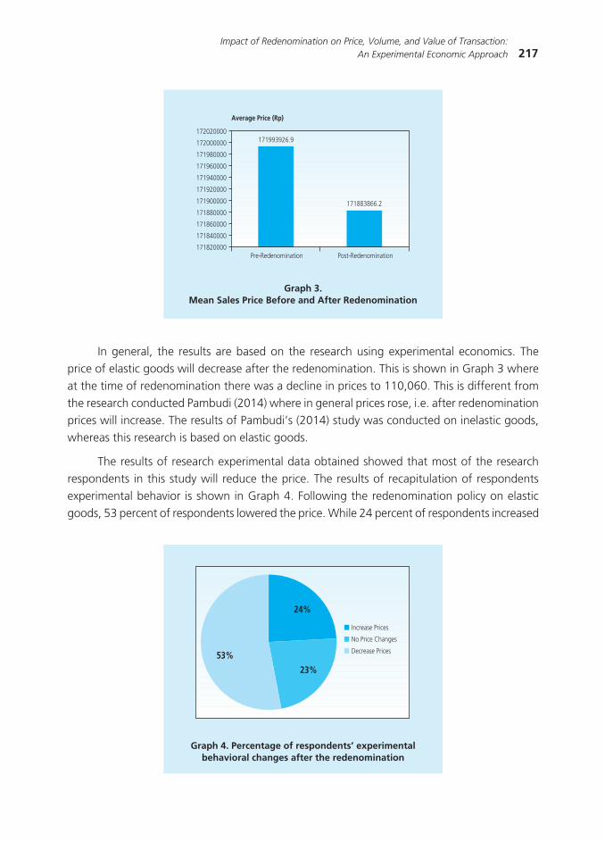
217Impact of Redenomination on Price, Volume, and Value of Transaction:
An Experimental Economic Approach
In general, the results are based on the research using experimental economics. The price of elastic goods will decrease after the redenomination. This is shown in Graph 3 where at the time of redenomination there was a decline in prices to 110,060. This is different from the research conducted Pambudi (2014) where in general prices rose, i.e. after redenomination prices will increase. The results of Pambudi’s (2014) study was conducted on inelastic goods, whereas this research is based on elastic goods.
The results of research experimental data obtained showed that most of the research respondents in this study will reduce the price. The results of recapitulation of respondents experimental behavior is shown in Graph 4. Following the redenomination policy on elastic goods, 53 percent of respondents lowered the price. While 24 percent of respondents increased
Graph 3.Mean Sales Price Before and After Redenomination
���������
���������
���������
���������
���������
���������
���������
���������
���������
���������
���������
������������������
������������� ���� �������������� ����
���������
���������
Graph 4. Percentage of respondents’ experimentalbehavioral changes after the redenomination
���
���
���
���������������
����������������
���������������
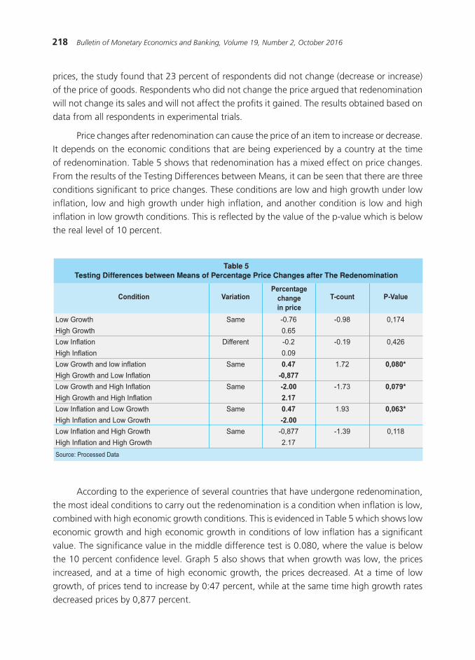
218 Bulletin of Monetary Economics and Banking, Volume 19, Number 2, October 2016
prices, the study found that 23 percent of respondents did not change (decrease or increase) of the price of goods. Respondents who did not change the price argued that redenomination will not change its sales and will not affect the profits it gained. The results obtained based on data from all respondents in experimental trials.
Price changes after redenomination can cause the price of an item to increase or decrease. It depends on the economic conditions that are being experienced by a country at the time of redenomination. Table 5 shows that redenomination has a mixed effect on price changes. From the results of the Testing Differences between Means, it can be seen that there are three conditions significant to price changes. These conditions are low and high growth under low inflation, low and high growth under high inflation, and another condition is low and high inflation in low growth conditions. This is reflected by the value of the p-value which is below the real level of 10 percent.
���������
����������������������������������������� ��������������������������������������� ������ �
����������������������������������������������������������������������������������������������������������������������������������������������������������������������������������������������������������������������������������������������������������������������������������������
�� �����������������
����
���������
����
����
����
����
���������������������
����������������������������������
�����
�����
����
����
���
��� �
����
����
������
������
���� �
�����
����������������
�������������
������� ������
According to the experience of several countries that have undergone redenomination, the most ideal conditions to carry out the redenomination is a condition when inflation is low, combined with high economic growth conditions. This is evidenced in Table 5 which shows low economic growth and high economic growth in conditions of low inflation has a significant value. The significance value in the middle difference test is 0.080, where the value is below the 10 percent confidence level. Graph 5 also shows that when growth was low, the prices increased, and at a time of high economic growth, the prices decreased. At a time of low growth, of prices tend to increase by 0:47 percent, while at the same time high growth rates decreased prices by 0,877 percent.
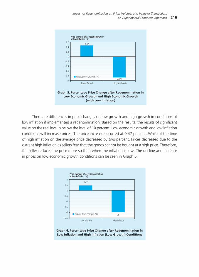
219Impact of Redenomination on Price, Volume, and Value of Transaction:
An Experimental Economic Approach
There are differences in price changes on low growth and high growth in conditions of low inflation if implemented a redenomination. Based on the results, the results of significant value on the real level is below the level of 10 percent. Low economic growth and low inflation conditions will increase prices. The price increase occurred at 0.47 percent. While at the time of high inflation on the average price decreased by two percent. Prices decreased due to the current high inflation as sellers fear that the goods cannot be bought at a high price. Therefore, the seller reduces the price more so than when the inflation is low. The decline and increase in prices on low economic growth conditions can be seen in Graph 6.
Graph 5. Percentage Price Change after Redenomination in Low Economic Growth and High Economic Growth
(with Low Inflation)
������������ �������������
����
������ �����������������������
��������������������������������������������������� ��
��
����
����
����
����
�
���
���
���
Graph 6. Percentage Price Change after Redenomination in Low Inflation and High Inflation (Low Growth) Conditions
�
���
�
����
��
����
��
����������������� �� �����������
���
�������������������� ������
��������������������������������������������������� ��
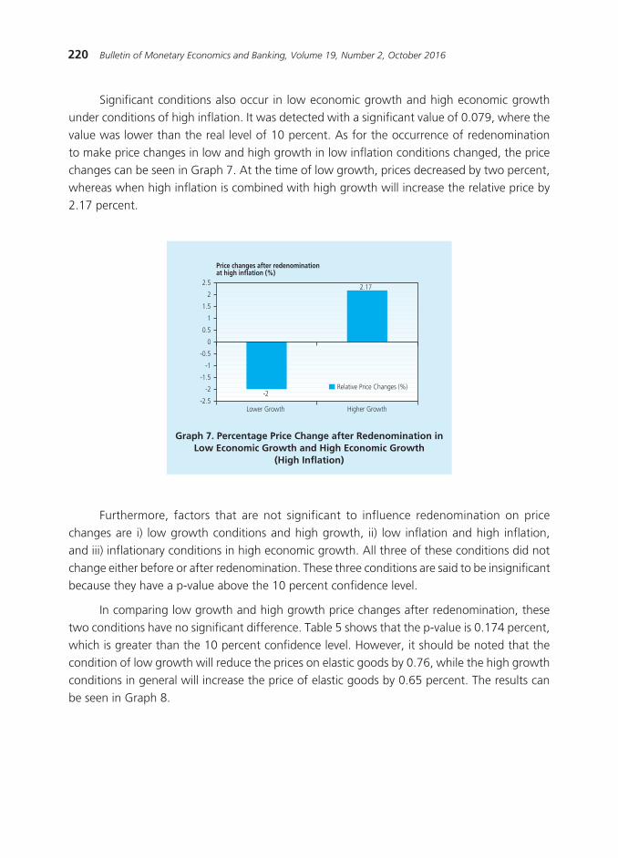
220 Bulletin of Monetary Economics and Banking, Volume 19, Number 2, October 2016
Significant conditions also occur in low economic growth and high economic growth under conditions of high inflation. It was detected with a significant value of 0.079, where the value was lower than the real level of 10 percent. As for the occurrence of redenomination to make price changes in low and high growth in low inflation conditions changed, the price changes can be seen in Graph 7. At the time of low growth, prices decreased by two percent, whereas when high inflation is combined with high growth will increase the relative price by 2.17 percent.
Graph 7. Percentage Price Change after Redenomination in Low Economic Growth and High Economic Growth
(High Inflation)
��
����
������������ �������������
�� ���������������������
����
��
����
��
����
�
���
�
���
�
���
����������������������������������������������������� �
Furthermore, factors that are not significant to influence redenomination on price changes are i) low growth conditions and high growth, ii) low inflation and high inflation, and iii) inflationary conditions in high economic growth. All three of these conditions did not change either before or after redenomination. These three conditions are said to be insignificant because they have a p-value above the 10 percent confidence level.
In comparing low growth and high growth price changes after redenomination, these two conditions have no significant difference. Table 5 shows that the p-value is 0.174 percent, which is greater than the 10 percent confidence level. However, it should be noted that the condition of low growth will reduce the prices on elastic goods by 0.76, while the high growth conditions in general will increase the price of elastic goods by 0.65 percent. The results can be seen in Graph 8.
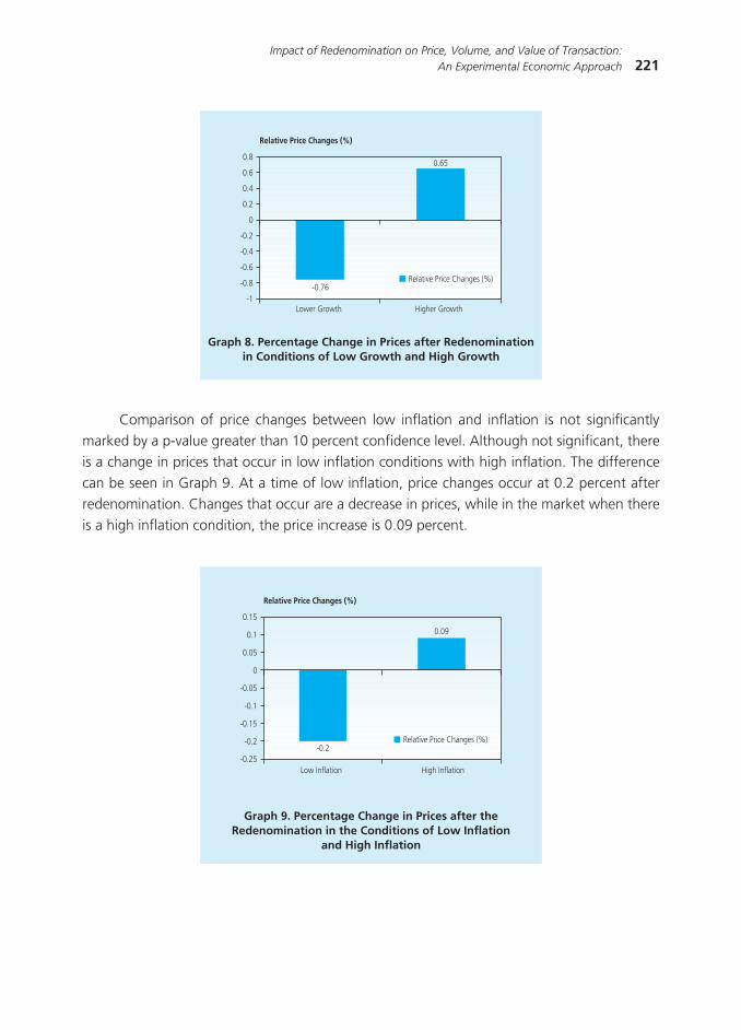
221Impact of Redenomination on Price, Volume, and Value of Transaction:
An Experimental Economic Approach
Comparison of price changes between low inflation and inflation is not significantly marked by a p-value greater than 10 percent confidence level. Although not significant, there is a change in prices that occur in low inflation conditions with high inflation. The difference can be seen in Graph 9. At a time of low inflation, price changes occur at 0.2 percent after redenomination. Changes that occur are a decrease in prices, while in the market when there is a high inflation condition, the price increase is 0.09 percent.
Graph 8. Percentage Change in Prices after Redenominationin Conditions of Low Growth and High Growth
Graph 9. Percentage Change in Prices after the Redenomination in the Conditions of Low Inflation
and High Inflation
�����
����
������������ ��������������
����
����
����
���
�
��
���
���
���
�������������������������
�������������������������
����
����
�����
����
�����
����
�����
�
����
���
����
������������� �������������
�������������������������
���������������������
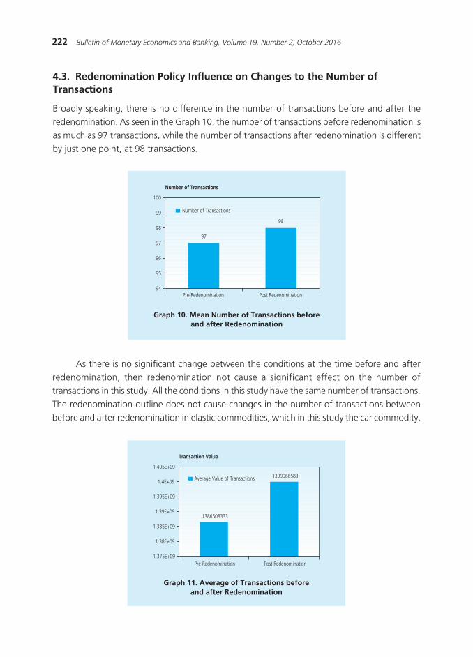
222 Bulletin of Monetary Economics and Banking, Volume 19, Number 2, October 2016
4.3. Redenomination Policy Influence on Changes to the Number of Transactions
Broadly speaking, there is no difference in the number of transactions before and after the redenomination. As seen in the Graph 10, the number of transactions before redenomination is as much as 97 transactions, while the number of transactions after redenomination is different by just one point, at 98 transactions.
Graph 10. Mean Number of Transactions beforeand after Redenomination
��
��
������������������ ���
��������� ��� �� ���������� ��� ����
��
��
��
��
��
���
����������������������
As there is no significant change between the conditions at the time before and after redenomination, then redenomination not cause a significant effect on the number of transactions in this study. All the conditions in this study have the same number of transactions. The redenomination outline does not cause changes in the number of transactions between before and after redenomination in elastic commodities, which in this study the car commodity.
Graph 11. Average of Transactions beforeand after Redenomination
����������
����������
�������������� ��� ��� ����������� ���
���������������������� ����
���������
��������
���������
��������
���������
�������
���������
�����������������

223Impact of Redenomination on Price, Volume, and Value of Transaction:
An Experimental Economic Approach
Overall this research found that the transaction value will increase after redenomination. In the beginning, the transaction value before redenomination had a value of 1,386,508,333 for elastic commodities. Meanwhile, after redenomination, the value increased to 1,399,966,583. The average result of the transaction value can be seen in Graph 11.
������
����������������������������������������������� ������������������������ �����������������������
������������������������
����������������������������������������������������������������������������������������������������������������������������������������������������������������������������������������������������������������������������������������������������������������������������������������
�� �����������������
����
����
���������
����
����
����
��������������������
�������
��������
������ ���
�� �
����
�� �
�����
����
�����
�����
�� ��
�����
������
�����
�����
������������� ���������
������������
������� �������
The value of transactions in the experimental studies increased in elastic commodities, which in this study are cars. The variance value of transactions in this study has mixed results, where there are significant conditions and insignificant conditions. Of the six treatment combinations, for significance value, there was only one condition of growth under high inflation conditions that showed significance. The combination of other conditions did not show a significant value below 10 percent.
The value of transactions in low growth and high growth did not differ significantly. It is seen from the p- value of 0406, where the value is above the 10 percent confidence value. The results are shown in Table 6. The redenomination can cause an increase in the value of the transaction in a state of low growth and high growth. Only at the time of low growth conditions, the increase of the transaction value is higher than at a time of high growth. At the time of high growth there is an increase of 0.65 per cent of the transaction value, while at the time of low growth conditions transactions increases amounted to 1.35 percent. This can be seen in Graph 12.
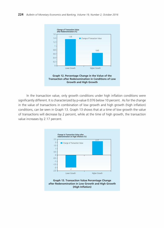
224 Bulletin of Monetary Economics and Banking, Volume 19, Number 2, October 2016
In the transaction value, only growth conditions under high inflation conditions were significantly different. It is characterized by p-value 0.076 below 10 percent. As for the change in the value of transactions in combination of low growth and high growth (high inflation) conditions, can be seen in Graph 13. Graph 13 shows that at a time of low growth the value of transactions will decrease by 2 percent, while at the time of high growth, the transaction value increases by 2.17 percent.
Graph 12. Percentage Change in the Value of theTransaction after Redenomination in Conditions of Low
Growth and High Growth
����
����
������������ ��������������
��
���
���
���
�
��
���
���
����������������������
��������������������������������� ���������������
Graph 13. Transaction Value Percentage Changeafter Redenomination in Low Growth and High Growth
(High Inflation)
��
��������������������� �������
����
��
����
��
����
�
���
�
���
�
���
���������� � ����������� �
����������������������������������� �������������������������������
225Impact of Redenomination on Price, Volume, and Value of Transaction:
An Experimental Economic Approach
V. CONCLUSIONS
Redenomination has a diverse impact if the policy is implemented by the government. The economic experiments conducted in this study examined the effects of redenominate on changes in the number of transactions, changes in transaction prices and changes in transaction value. Based on the research results, redenominate can significantly change the transaction price. The greatest decline in transaction prices for most elastic goods occurs when low growth conditions are combined with high inflation, and when high growth conditions are combined with low inflation.
Change in the number of transactions is not significant in this study. There is no change in the number of transactions before and after the redenomination on elastic goods. With regards to transaction values, there is a significant change if it is done under conditions of high growth combined with high inflation.
Judging from the results, the prevailing economic conditions of a country at the time of currency redenomination policy implementation is important. Redenomination is better applied when the economy is in good and stable condition, such as the low inflation and high economic growth rate. The dissemination redenomination policy to the public needs to be done before consistently and with intensity to provide clear information to the public related to the policy.
It is expected that in further research that will be done next, researchers can add responses to economic experiments and perform other transaction systems. This could include added responses such as interest rates and socialization to the community. While a transaction system can also be added, if in this study is implemented Posted Offer, then further research can use a decentralized system or bargain (double auction) system.
226 Bulletin of Monetary Economics and Banking, Volume 19, Number 2, October 2016
REFERENCES
Amir, Amir. “Redenominasi Rupiah dan Sistim Keuangan”, Journal of Paradigma Ekonomika, October 2011, Vol.1, No.4.
Friedman. D and Sunder, (1994), Experimental Methods : A Premier for Economist. Cambridge University Press, Melbourne.
Gamble. A, Garling. T, Charlton. J, & Ranyard. R, Euro Illusion, European Psychologist 7, (2002), 4: 302-311.
Hobijn. Bart, F. Ravena, and A. Tambalotti, “Menu Costs at Work: Restaurant Prices and the Introduction of the Euro”, The Quarterly Journal of Economics, 2006, 121 (3): 1103-1131.
Ioana. D, (2005), The National Currency Re-denomination Experience in Several Countries: A
Comparative Analysis, International Multidisciplinary Symposium Universitaria Simpro.
Juanda. B, (2009), Metodologi Penelitian Ekonomi dan Bisnis, IPB Press, Bogor.
Juanda. B, (2010), Ekonomi Eksperimental untuk Pengembangan Teori Ekonomi dan Pengkajian
Suatu Kebijakan: Speech of The Board of Professors IPB, 25 September 2010.
Juanda. B, (2012), Experimental Economics in Indonesia: Lesson Learned and Best Practices, Workshop on Experimental Economics, Bogor 6 September 2012.
Juanda. B, N. Fitri, F. Fardilah, and M.P.D. Manik, (2010), Analisis Perbandingan Dampak
Kebijakan Menyelamatkan Bank Century dengan kebijakan Menutup Bank Century dengan
Metode Eksperimen, Department of Economic Science, FEM-IPB, Bogor.
Kesumajaya. IWW, (2011) “Redenominasi Mata Uang Rupiah Merupakan Bagian dari Tugas Bank
Indonesia untuk Mengatur dan Menjaga Kelancaran Sistim Pembayaran di Indonesia”,
February 2011, GaneC Swara Vol 5 No.1.
Lianto. J and Suryaputra. R, (2012), The Impact of Redenomination in Indonesia from Indonesian
Citizens’ Perspective. Proceeding - Social and Behavioral Sciences 40 (2012): pp. 1 – 6.
Marques. JF and Dehaene. S, (2004), “Developing Intuition for Price in Euros”, Journal of Experimental Psychology, 2004, 10, 3: 148-155.
Mehdi. S and Motiee. R, (2012) “An investigating Zeros Elimination of the National Currency
and Its Effect on National Economy (Case study in Iran”). European Journal of Experimental Biology, 2012, 2 (4):1137-1143.

227Impact of Redenomination on Price, Volume, and Value of Transaction:
An Experimental Economic Approach
Mosley. L, (2005), Dropping Zeros, Gaining Credibility? Currency Redenomination in Developing
Nations, Annual Meeting of The American Political Science Association, 2005, Washington DC.
Pambudi. Andika, (2014), Faktor-faktor yang Memengaruhi Keberhasilan Redenominasi Mata Uang: Pendekatan Historis dan Eksperimental, Thesis, Postgraduate School of IPB.
Press Release of Bank Indonesia No. 12/38/PSHM/Humas.
Suhendra. E dan S.W. Handayani, (2012), Impacts of Redenomiantion on Economics Indicators, International Conference on Eurasian Economies 2012.
Wibowo. B, (2013), “Ilusi Nilai Uang Redenominasi”, Business Daily Kontan, Thursday 21 February 2013.

228 Bulletin of Monetary Economics and Banking, Volume 19, Number 2, October 2016
This page intentionally left blank

MANUSCRIPT TERMS OF DELIVERY
1. The manuscript must be an original work of the author (individuals, groups or institutions) that do not infringe copyright. The submitted manuscript has never been published and is not being sent to other publishers at the same time. The copyright of the received manuscript is the author’s.
2. Each approved manuscript will receive Rp 5.000.000,- financial compensation.
3. The manuscript template can be downloaded at www.journalbankindonesia.org/index.php/BEMP
4. Manuscripts can be submitted in softcopy (file). We strongly suggest to send your softcopy to:
[email protected] (Cc. to: [email protected].)
5. Manuscripts can also be sent via www.journalbankindonesia.org
6. Mathematical equations and symbols are written using Microsoft Equation.
7. Each manuscript should include abstract, a maximum of one (1) page size A4. For Indonesian manuscript, the abstract should be in English and vice versa.
8. The manuscript must include keywords and two-digit classification numbers of the Journal of Economic Literature (JEL). Please refer to JEL classification, http://www.aeaweb.org/journal/jel_class_system.html.
9. The manuscript must include author’s bio (address, phone number, bank account and e-mail). It is suggested to write the biographical data in the form of a complete CV (curriculum vitae).

230 Bulletin of Monetary Economics and Banking, Volume 19, Number 2, October 2016
This page intentionally left blank