BUCKLING OF PIPELINES DUE TO INTERNAL PRESSURE · the deflected pipeline (one half-wave buckling...
20
CILAMCE 2016 Proceedings of the XXXVII Iberian Latin-American Congress on Computational Methods in Engineering Suzana Moreira Ávila (Editor), ABMEC, Brasília, DF, Brazil, November 6-9, 2016 BUCKLING OF PIPELINES DUE TO INTERNAL PRESSURE Marina V. Craveiro Alfredo Gay Neto [email protected] [email protected] Department of Structural and Geotechnical Engineering, Polytechnic School at University of São Paulo Av. Prof. Almeida Prado, trav. 02, nº 83. São Paulo, SP, Brazil Abstract. The pipelines used to transport oil and gas tend to expand due to high temperature and pressure conditions. If this expansion is inhibited, a compressive axial force arises. The pipeline can relieve the stresses by lateral or upheaval buckling. The objective of the present work is to analyze the instability of pipelines due to internal pressure, experiencing different boundary conditions and imperfection magnitudes. It aims at discussing the equivalence between approaches that involve the application of the load as the internal pressure and as an equivalent compression with follower and non-follower characteristics, besides discussing the influence of using static or dynamic analysis for such approaches. The methodology involves the development of geometrically-simple Timoshenko beam structural models. To perform the simulations, Giraffe finite element software is used for nonlinear analysis. The study presents comparisons between critical forces and post-buckling configurations for the different boundary conditions, imperfections, load types and analysis methods considered, as well as comparisons between numerical and analytical solutions. Through the study, it is concluded that the equivalence in results between the distinct approaches depends on the nature of boundary conditions. Keywords: Buckling, Effective axial force, Internal pressure, Nonlinear analysis, Pipeline
Transcript of BUCKLING OF PIPELINES DUE TO INTERNAL PRESSURE · the deflected pipeline (one half-wave buckling...

CILAMCE 2016 Proceedings of the XXXVII Iberian Latin-American Congress on Computational Methods in Engineering
Suzana Moreira Ávila (Editor), ABMEC, Brasília, DF, Brazil, November 6-9, 2016
BUCKLING OF PIPELINES DUE TO INTERNAL PRESSURE
Marina V. Craveiro
Alfredo Gay Neto
Department of Structural and Geotechnical Engineering, Polytechnic School at University of
São Paulo
Av. Prof. Almeida Prado, trav. 02, nº 83. São Paulo, SP, Brazil
Abstract. The pipelines used to transport oil and gas tend to expand due to high temperature
and pressure conditions. If this expansion is inhibited, a compressive axial force arises. The
pipeline can relieve the stresses by lateral or upheaval buckling. The objective of the present
work is to analyze the instability of pipelines due to internal pressure, experiencing different
boundary conditions and imperfection magnitudes. It aims at discussing the equivalence
between approaches that involve the application of the load as the internal pressure and as an
equivalent compression with follower and non-follower characteristics, besides discussing the
influence of using static or dynamic analysis for such approaches. The methodology involves
the development of geometrically-simple Timoshenko beam structural models. To perform the
simulations, Giraffe finite element software is used for nonlinear analysis. The study presents
comparisons between critical forces and post-buckling configurations for the different
boundary conditions, imperfections, load types and analysis methods considered, as well as
comparisons between numerical and analytical solutions. Through the study, it is concluded
that the equivalence in results between the distinct approaches depends on the nature of
boundary conditions.
Keywords: Buckling, Effective axial force, Internal pressure, Nonlinear analysis, Pipeline

Buckling of pipelines due to internal pressure
CILAMCE 2016 Proceedings of the XXXVII Iberian Latin-American Congress on Computational Methods in Engineering
Suzana Moreira Ávila (Editor), ABMEC, Brasília, DF, Brazil, November 6-9, 2016
1 INTRODUCTION
This section presents the motivation, the literature review, the objectives and the
methodology of the work.
1.1 Motivation
In the productive chain of oil and gas, providing from onshore and offshore fields, once
performed the extraction, it is necessary to transport the fluid to the points of distribution and
refining. Such transportation is made predominantly by pipelines. Specifically in the case of
subsea pipelines, according to Bai and Bai (2014), the term of subsea flowlines is used to
describe subsea pipelines that transport oil and gas from the wellhead to the riser base. The
riser, in its turn, is connected to the processing facilities. Finally, the transportation from there
to shore is performed by export pipelines.
Since the oil and gas fields have high pressure and high temperature, the fluids usually
leave the reservoir still keeping such thermodynamic state during the transportation. If it
changes, wax and hydrate may be formed as the fluid cools along the pipeline, which is not
desired. Therefore, in order to make the transportation described previously more efficient, it is
necessary that the pipelines operate at high pressure and temperature conditions, reaching levels
above 150 oC and 70 MPa. Such conditions are becoming more and more severe since the oil
and gas industries are advancing and discovering new reserves, especially in deep water regions
away from the continent. The pipelines under the conditions commented are called high
pressure and high temperature pipelines (HPHT pipelines).
Among other implications of HPHT operation in pipelines, the tendency of longitudinal
expansion can be cited. This expansion may generate a compressive axial force, since it is
partially or totally inhibited by existing restrictions to movement at the pipe ends and along the
contact with the ground. When the compressive axial force reaches a certain critical level of
magnitude, the pipeline may relieve the stresses by means of two types of buckling: lateral
buckling and upheaval buckling. The first type is more common in pipelines which are just laid
on the seabed. The second type, in its turn, is more common in buried pipelines, since the lateral
resistance generated by the soil becomes larger in this case.
Both aforementioned cases consist in global phenomena and, by themselves, do not
correspond to failure modes. However, the buckling of pipelines can propitiate, by excessive
bending, the occurrence of failures like local buckling, fracture and fatigue. The local buckling
occurs due to the combination of longitudinal forces, pressure and bending. It can occur by
yielding of the cross section or buckling on the compressive side of the pipe. The fracture is
caused by excessive tensile strains and can include brittle fracture and plastic collapse. Finally,
the fatigue occurs due to cyclic loads like the generated by the vortex induced vibration (VIV),
pressures, thermal and hydrodynamic loads (Fan, 2013). Such failure modes may cause serious
accidents since the fluid that is transported may leak and contaminate the environment. In 2000,
for example, in Guanabara Bay (Brazil), the lateral buckling caused local buckling and fracture
in the wall of the Petrobras’ pipeline PE-II, leaking 1300 cubic meters of oil. This accident
occurred due to an erosion that uncovered the pipeline, allowing it to move laterally (Cardoso,
2005).
In this context, studies related to buckling of pipelines are justified, because this
phenomenon may lead to structural damages that may cause accidents. Accidents have
disastrous consequences for the economy and the environment. Thus, their probability of
occurrence has to be minimized.

Marina V. Craveiro, Alfredo Gay Neto
CILAMCE 2016 Proceedings of the XXXVII Iberian Latin-American Congress on Computational Methods in Engineering
Suzana Moreira Ávila (Editor), ABMEC, Brasília, DF, Brazil, November 6-9, 2016
1.2 Literature review
There are many lines of research about buckling of pipelines that have been developed in
the last decades. Among these lines of research are those concerning the buckling description,
those concerning the influence of imperfections on buckling and those concerning the
alternatives to minimize the effects of buckling. Such works include both analytical and
numerical analyses. In this section, some researches will be summarized in order to
contextualize the objectives of the present work.
Hobbs (1984) was one of the first researchers to deal with buckling specifically in
pipelines. His work involves studies about upheaval buckling and lateral buckling. For the
upheaval buckling, Hobbs (1984) assumes the pipeline as a Bernoulli-Euler beam that is
subjected to an axial force and to its self-weight and considers that the problem is elastic linear
with small slopes. Besides this, Hobbs (1984) considers that the contact with the soil is rigid
and the friction is fully mobilized. The analysis consists in solve the differential equation for
the deflected pipeline (one half-wave buckling mode). Considering that the term of buckle
refers to the deformed configuration of the pipeline, the results are the expressions for: critical
buckling load, axial load in the buckle, buckle length, slipping length, maximum amplitude of
the buckle, maximum bending moment and maximum slope. The same procedure is performed
for lateral buckling and the same kind of results is obtained. The difference between the two
cases is in the fact that the author, to simplify the study, adopts a buckling mode with infinite
series of half waves to derive the aforementioned expressions for lateral buckling, since the
contact of the pipeline with the soil cannot be considered rigid in this case.
With the mathematical formulations of the two cases presented, Hobbs (1984) also presents
numerical examples experiencing several friction coefficients between the pipe and the soil.
The results are graphics that relate buckle amplitudes and buckle lengths to the corresponding
temperature rise in the pipeline. The author concludes that lateral buckling occurs with smaller
compressive forces than upheaval buckling. These results are inverted if the pipeline is buried.
It is worth mentioning that Hobbs (1984) does not consider imperfections in his models,
although the author highlights its importance since perfect pipelines do not buckle and actual
pipelines have imperfections.
Considering the need for researches in the field pointed by Hobbs (1984), Taylor and Gan
(1986) perform similar analyses to the work of the previous author. They study both upheaval
buckling and lateral buckling for some buckling modes and assume small deflections and elastic
linear behavior for the material. In their work, however, there is the consideration of structural
imperfections. These imperfections can be, for example, irregularities of seabed or initial out-
of-straightness providing from laying operations. It is worth mentioning that the imperfection
that is considered is totally in contact with the pipeline. Beyond the consideration of such
imperfections, to become the model more realistic, the authors consider a deformation-
dependent axial friction, that is, the friction is not fully mobilized.
After showing the mathematical expressions to determine critical buckling load, axial load
in the buckle, maximum amplitude of the buckle, maximum bending moment and maximum
compressive stress for lateral and upheaval buckling, Taylor and Gan (1986) perform numerical
assessments for a range of imperfection amplitudes, generating, as well as Hobbs (1984),
graphics that relate buckle amplitudes and buckle lengths to the corresponding temperature rise
in the pipeline. The work concludes that the cases with small imperfections have larger critical
loads than the cases with large imperfections, but small imperfections cause abrupt
displacements when the critical load is reached. As the imperfections increase, the critical loads
decrease and the equilibrium paths become more stable.
Buckling of pipelines due to internal pressure
CILAMCE 2016 Proceedings of the XXXVII Iberian Latin-American Congress on Computational Methods in Engineering
Suzana Moreira Ávila (Editor), ABMEC, Brasília, DF, Brazil, November 6-9, 2016
Taylor and Tran (1996) also discuss imperfections in their work, focusing on the upheaval
buckling. The authors divide the isolated imperfections in three different types. The first
imperfection is that in which the pipeline is totally in contact with the ground. The second type,
on the other hand, is an imperfection that is not totally in contact with the ground. Thus, there
are voids between the pipe and the seabed. Finally, the third type consists in the second type of
imperfection, but, in this case, the voids become filled by sand or other marine materials. Taylor
and Tran (1996) focus on the second type of imperfection, presenting a mathematical
formulation that considers the following assumptions: the imperfections are symmetrical, the
soil is rigid, the deflections are small, the material is elastic linear and the initially deformed
pipeline does not have stresses (since these stresses cannot be determined with accuracy). The
mathematical model proposed by the authors also can be used for buried pipelines. According
to Taylor and Tran (1996), who have also performed numerical case studies, the results are
similar to existing experimental data and, as proposed by Taylor and Gan (1986), the
imperfections have great influence on critical load, making it smaller. To make the discussions,
graphics of temperature rise versus buckle amplitudes/lengths are presented.
Ballet and Hobbs (1992) study upheaval buckling in pipelines that find a point of
irregularity in the seabed. Firstly, the authors analyze the approximations performed by
Richards and Andonicou (1986 apud Ballet; Hobbs, 1992) in the symmetrical upheaval
buckling of pipelines over ground imperfections. These approximations consist in: do not
consider concentrated forces at the points in which the pipeline loses its contact with the soil in
the calculus of the boundary displacement strain and consider a sinusoidal deformed
configuration in the calculus of the arclength strain instead of integrating the general expression
of the slope in the buckle to calculate such strain. According to Ballet and Hobbs (1992), these
approximations underestimate the critical load. Besides presenting the revised formulation
without approximations, Ballet and Hobbs (1992) presents the possibility of asymmetrical
buckling. The results indicate that critical loads are smaller in the asymmetrical case. Again,
the analysis is based on graphics of temperature rise versus buckle amplitudes.
Recent studies, besides analytical analysis, propose numerical analysis with finite element
method (FEM). With the analysis by FEM, it is possible to simulate more complex and more
realistic models of pipelines that could not be solved by analytical methods. The contact
between the pipe and the soil, for example, can be simulated using arbitrary seabed profiles.
Furthermore, it is possible to simulate nonlinear material properties and use large deflection
theory (physical and geometrical nonlinearities, respectively).
For the first case proposed by Taylor and Tran (1996), for example, Liu, Wang and Yan
(2013), besides analytical formulation, develop an elastoplastic analysis for the pipeline
buckling using FEM. The authors apply such methods in a practical case in China. The study is
made based on temperature rises that play the role of temperature and pressure increases,
jointly. The conclusions of the work are similar to those reached by the other researches: the
critical load depends on the imperfection amplitude. Furthermore, for equal imperfection
amplitudes, the critical load is larger when the covered depth and the soil strength are larger.
The work of Zeng, Duan and Che (2014), in its turn, simulates, using FEM, the upheaval
buckling of pipelines for three different groups of imperfection. It is worth mentioning that the
research considers parameters as the imperfection amplitude, the imperfection length and the
imperfection shape to define the groups. Based on comparisons between the three groups of
imperfection, the authors conclude that when the rate between the imperfection amplitude and
the imperfection length increases, buckling occurs with smaller critical loads and less abruptly.
The same occurs for compacted imperfections. The authors also propose approximated
formulas to determine the critical loads for the analyzed imperfections.

Marina V. Craveiro, Alfredo Gay Neto
CILAMCE 2016 Proceedings of the XXXVII Iberian Latin-American Congress on Computational Methods in Engineering
Suzana Moreira Ávila (Editor), ABMEC, Brasília, DF, Brazil, November 6-9, 2016
An aspect that is worth to be discussed is that all works exposed previously do not analyze
the effects of internal pressure specifically. Although they have comments about pressure,
Hobbs (1984), Taylor and Gan (1986), Taylor and Tran (1996), Ballet and Hobbs (1992), Liu,
Wang and Yan (2013), and Zeng, Duan and Che (2014) analyze the critical load just in terms
of critical temperature rise. Liu, Wang and Yan (2013), by the way, consider that part of the
temperature rise refers to pressure. It can be said that such works are concerned about the critical
load as a whole. In other words, the objective is not to distinguish the effects of temperature
and pressure, but to have some kind of practical measure for the critical load. Thus, the previous
studies could also be made in terms of pressure. Other researches, however, simulate practical
cases of pipelines, applying both temperature and pressure load. In such cases, the objective is
usually to know if certain pipelines are or not likely to buckle. Isaac (2013), for example,
analyzes a specific case study with pipe-soil contact and temperature and pressure loads. The
objective is to know if the pipeline buckles and what is the better lay configuration that would
allow controlling the pipeline buckling. Therefore, one more time, the effects of pressure are
not analyzed separately.
To finalize this literature review, it is important to show one of the few works that deal
mainly with the pressure in pipes. Dvorkin and Toscano (2001) analyze the global buckling in
pipelines that are subjected to internal and external pressures, besides compressive axial forces
(it can be associated with temperature, for example). According to Dvorkin and Toscano (2001),
imperfect pipelines have a resultant force providing from pressure loads that has a tendency to
modify the pipe curvature. When internal pressure is larger than external pressure, it results in
a destabilizing load pointing from the center of curvature and the critical load is smaller than
the critical load in perfect pipelines. The inverse situation, in its turn, generates a stabilizing
load and the critical load is larger than the critical load in perfect pipelines. Considering these
aspects, Dvorkin and Toscano (2001) propose analytical expressions for cylindrical pipes
without imperfections and finite element models for elastoplastic imperfect pipes. The
conclusion is that smaller imperfections cause critical loads closer to critical loads of perfect
pipelines than larger imperfections.
1.3 Objectives and methodology
From Section 1.2, it can be noted that the advanced techniques of numerical simulations
allow more realistic analyses of buckling of pipelines. The several lines of research that were
shown in that section are still being improved and new aspects are being included (soil-pipe
interaction, elastoplastic material behavior and alternatives to mitigate buckling, for instance).
Therefore, buckling of pipelines is an important phenomenon in which researches still have
field of work. However, it can also be highlighted, about everything, the lower amounts of
studies that just analyze the effects of internal pressure in the buckling of pipelines.
Motivated by this context, the objective of the present work is to analyze the instability of
pipelines due to internal pressure, experiencing different boundary conditions and imperfection
magnitudes. It aims at discussing the equivalencies between approaches that involve the
application of the load as the internal pressure and as an equivalent compression with follower
and non-follower characteristics, besides discussing the influence of using static or dynamic
analysis for such approaches. The study presents comparisons between critical forces and post-
buckling configurations for the different boundary conditions, imperfections, load types and
analysis methods considered, as well as comparisons of the results obtained by numerical
simulations with existing analytical solutions. For that, the study involves the development of
geometrically-simple models using Timoshenko beam structural model. Therefore, the
intention of this work is not to simulate complex models, but to understand the phenomenon of

Buckling of pipelines due to internal pressure
CILAMCE 2016 Proceedings of the XXXVII Iberian Latin-American Congress on Computational Methods in Engineering
Suzana Moreira Ávila (Editor), ABMEC, Brasília, DF, Brazil, November 6-9, 2016
buckling due to internal pressure for several simple cases, real or hypothetical.
To perform simulations, it is used the finite element software for nonlinear analysis Giraffe
(Generic Interface Readily Accessible for Finite Elements), under continuous development at
the University of São Paulo. This software has an own formulation for the application of the
internal pressure load in the beam elements. It applies such pressure load as an equivalent
distributed load, implying in less computational cost and more easiness to perform the
simulations. The detailed formulation can be found in the paper accepted by Journal of
Engineering Mechanics (Gay Neto; Martins; Pimenta, 2016).
2 THEORETICAL DISCUSSIONS
To understand more easily the role of pressure in buckling and to relate the axial critical
force to pressure, it is necessary to understand the effective axial force concept. It is exposed
with more details in this section since it will be largely used in this work. In this section,
theoretical aspects and some cases of structural stability will be also summarized in order to
have a better understanding of the results obtained in this work.
2.1 Effective axial force
It is important to have in mind that the effects of internal and external pressures in pipelines
can be analyzed by their integration on the internal and external wall sections of the pipeline,
respectively. However, this procedure requires a lot of algebraic work depending on the pipe
geometry, such as dealing with curved pipe configurations. Thus, another way for considering
the pressure effects in the pipeline buckling is analyzing an equivalent force in the axial
direction related to pressure loads. This approach, although easier, has to be used with caution
since its physical interpretation is non-direct. For example, pipelines without end caps and just
subject to internal pressure have the tendency of contraction in the axial direction. It happens
because the existing tensile hoop strain generates, by Poisson effect, a compressive strain in the
axial direction, if there is no restriction in the pipe. However, when the axial movement of the
pipe is restricted in practical situations, a tensile stress arises in the pipe. In this way, sometimes
it is difficult to understand why pipelines buckle due to internal pressure. Actually, the force
that governs the buckling of pipelines is not the real force given by the integration of the stresses
on the cross section. This phenomenon is governed by the called effective axial force, which
becomes compressive due to internal pressure. Therefore, there are other pressure effects in the
pipeline axial direction besides the contribution of the Poisson effect.
Sparks (1984) introduces the term of effective axial force. Fyrileiv and Collberg (2005), in
their turns, summarize the knowledge about the topic. For the next discussions, based on the
studies of the previous authors, consider the pipe segment shown in Fig. 1 and the following
notation: δL is the pipe segment length, Wt is the pipe segment true weight per unit length, pe is
the external pressure, pi is the internal pressure, Ttw is the true axial force in the pipe wall (as a
result of the stresses integration on a pipe cross section), Se is the external cross section at the
pipe ends, Si is the internal cross section at the pipe ends, ρi is the specific mass of the internal
fluid, ρe is the specific mass of the external fluid, Di is the internal diameter of the cross section
and De is the external diameter of the cross section.

Marina V. Craveiro, Alfredo Gay Neto
CILAMCE 2016 Proceedings of the XXXVII Iberian Latin-American Congress on Computational Methods in Engineering
Suzana Moreira Ávila (Editor), ABMEC, Brasília, DF, Brazil, November 6-9, 2016
Figure 1. Equivalent systems for pipelines subjected to internal and external pressures
A pipe segment without end caps and subjected to internal and external pressures is not a
closed pressure field. Therefore, the Archimedes’ principle cannot be applied. To apply such
principle is necessary to transform the original pipe physical system in an equivalent sum of
three different pipe physical systems. The first of the three physical systems is a closed pipe on
which acts the external pressure. By the Archimedes’ principle, the action of the external
pressure is equivalent to an upward-directed force. The magnitude of this force is the weight of
the external fluid displaced by the pipe segment (the buoyancy of the pipe). The second system
is a closed pipe on which acts the internal pressure. The action of the internal pressure is
equivalent to a downward-directed force. The magnitude of this force is the weight of the
internal fluid. Finally, the last physical system is a closed pipe on which act, besides the pipe
true weight and the true axial force, pressures at the pipe ends. These pressures have the
opposite sign to those applied in the first and in the second physical systems. Thus, these
pressures compensate the additional terms included in the first and in the second physical
systems. The paper accepted by Journal of Engineering Mechanics (Gay Neto; Martins;
Pimenta, 2016) discusses the three systems commented performing the integration of the
pressures on the internal and external wall sections of the pipeline.
The effective axial force (Te) is the resultant axial force at the pipe segment ends, with (+)
for tension and (-) for compression:
𝑇𝑒 = 𝑇𝑡𝑤 + 𝑝𝑒𝑆𝑒 − 𝑝𝑖𝑆𝑖 (1)
In practical cases, the term called true axial force (Ttw) can be composed, for example, by
the contributions of the axial effect of temperature, the axial effect of soil friction and the axial
effect of pressure (the Poisson effect and the end cap effect – if there are end caps in the pipes
indeed). The present work has the objective to analyze just the internal pressure effects in the
pipeline buckling. Thus, the term peSe will be disregarded. Furthermore, Timoshenko beam
models will be used to represent the pipelines. These beams have the assumption that the cross
sections are rigid and the Poisson effect is not considered for the pressure load. Besides this,
the pipelines considered do not have end caps. Therefore, the term Ttw could appear only due to
the action of other external loads, such as axial external forces, which would generate non-null
true wall tension in the pipe. Simplifying the Eq. (1), it results in:
𝑇𝑒 = 𝑇𝑡𝑤 − 𝑝𝑖𝑆𝑖 (2)

Buckling of pipelines due to internal pressure
CILAMCE 2016 Proceedings of the XXXVII Iberian Latin-American Congress on Computational Methods in Engineering
Suzana Moreira Ávila (Editor), ABMEC, Brasília, DF, Brazil, November 6-9, 2016
2.2 Stability of structures
General discussions. Once determined the internal pressure or the equivalent axial force
acting on the pipe, it is necessary to know if the pipeline buckles when subjected to these loads.
Moreover, if the pipe buckles, it is necessary to know what is the magnitude of its displacements
after the buckling. Clearly, this scenario consists in a stability problem, because the focus is on
the load for which the pipe loses the stability of its initial configuration and tries to find another
stable configuration. For this reason, some aspects of stability of structures will be presented in
this section. The intention of this section, however, is not to discuss stability of structures
deeply, but to discuss simple ideas that will be the basis of comparison between analytical and
numerical solutions in Section 3. Basically, the present work is concerned about critical loads
and post-buckling configurations.
There are several methods to analyze stability problems. Ziegler (1968), for instance,
discusses four methods to deal with such problems. According to the author, the first method is
called imperfection method and consists in analyzing the behavior of imperfect structures. The
main idea of this method is to determine the load for which the static displacements become
excessive or infinite (in the linear case). The equilibrium method, the second of the four
methods presented by Ziegler (1968), consists in analyzing the equilibrium of perfect structures.
When the trivial equilibrium position loses its stability, a nontrivial equilibrium position
appears. Therefore, the equilibrium method looks for the loads for which such perfect structures
admit nontrivial equilibrium configurations. The third method, in its turn, is based on the
potential energy of the system. The transition from stability to instability may occur when the
potential energy ceases to be positive definite (or ceases to be a point of minimum). According
to Bazant and Cedolin (2010), the second method represents a part of the third method,
however, the second method does not answer the question of stability: it gives only equilibrium
states, which may be stable or not. It is also worth mentioning that all such methods have a
static-assumption nature for the structure equilibrium. The last method presented by Ziegler
(1968), however, is kinetic. The called vibration method establishes that, in stable systems,
small perturbations result in bounded motions in the vicinity of the equilibrium position. Thus,
the idea of this method is to find the load for which such motions become unbounded.
Ziegler (1968) also shows that both static and dynamic methods provide the same critical
loads for the Euler’s column buckling problems. However, this conclusion cannot be
generalized for all systems. The author, by the way, discusses some cases in which such
conclusion is not true. A question that arises is when the static and dynamic methods should be
used. Besides Ziegler (1968), Bazant and Cedolin (2010) and Gay Neto and Martins (2013) also
address the question. To understand the topic, it is fundamental to list what are the types of
force that can act on a physical system. In general, the forces can be divided into active forces
(loads) and reactive forces (reactions). The reactions, in systems whose constraints do not
depend on time, can be either nonworking or dissipative. The loads, in their turns, can be
divided into non-stationary and stationary loads. The stationary loads can be subdivided into
loads which depend on velocity (gyroscopic and dissipative loads) and loads which do not
depend on velocity (circulatory and non-circulatory loads). Some of the forces described can
be classified as conservative: the nonworking reactions, the gyroscopic loads and the non-
circulatory loads. According to Ziegler (1968), the work of conservative forces depends
exclusively on the initial and final configurations of the system.
Based on such classification and on the works cited previously, it is possible to outline the
situations in which static and dynamic analyses are valid. Some aspects can be summarized as
follows: conservative and non-gyroscopic systems (in which act conservative forces but do not

Marina V. Craveiro, Alfredo Gay Neto
CILAMCE 2016 Proceedings of the XXXVII Iberian Latin-American Congress on Computational Methods in Engineering
Suzana Moreira Ávila (Editor), ABMEC, Brasília, DF, Brazil, November 6-9, 2016
act gyroscopic forces) can be analyzed by both static and dynamic methods; purely dissipative
systems (in which act only conservative and dissipative forces) can be analyzed by both static
and dynamic methods; usually circulatory systems (in which act circulatory forces) and non-
stationary systems (with non-stationary forces) cannot be analyzed by static methods. Bazant
and Cedolin (2010) state that the dynamic analysis consists in the fundamental test of stability,
but the static analysis brings useful simplifications and should be used whenever possible and
convenient.
Examples. To illustrate the aforementioned discussions, two examples, based on Ziegler
(1968), are discussed in this section (Fig. 2). They consist in prismatic cantilever columns with
flexural rigidity EI and elastic linear material behavior. There is also an assumption of small
strains and small deflections. The first case has a non-follower load P at the free end and will
be discussed by equilibrium method. The second case has a follower load P at the free end and
will be discussed by equilibrium and vibration methods. The notation (…)’ stands for the
derivative with respect to x coordinate.
Figure 2. Cantilever columns with non-follower and follower load, respectively (ZIEGLER, 1968)
Starting by the first case and assuming that the eccentricity e is zero (since the equilibrium
method deals with perfect systems), the linearized equation of the deflection curve and the
boundary conditions, with f being the deflection at the free end x = l, are:
𝐸𝐼𝑦" = 𝑃(𝑓 − 𝑦) (3)
𝑦 (0) = 𝑦′(0) = 0; 𝑦 (𝑙) = 𝑓 (4)
The general solution of Eq. (3) is:
𝑦 = 𝐴𝑐𝑜𝑠((𝑃/𝐸𝐼)0.5𝑥) + 𝐵𝑠𝑖𝑛((𝑃/𝐸𝐼)0.5𝑥) + 𝑓 (5)
The boundary conditions, in their turns, require that:
𝐴𝑐𝑜𝑠((𝑃/𝐸𝐼)0.5𝑙) = 0 (6)
Thus, the loads for which the column admits nontrivial equilibrium positions are:
𝑃𝑚 = 𝑚2𝜋2𝐸𝐼/4𝑙2 (7)
The same procedure can be done for other boundary conditions in the first case. The results
are summarized in Table 1.

Buckling of pipelines due to internal pressure
CILAMCE 2016 Proceedings of the XXXVII Iberian Latin-American Congress on Computational Methods in Engineering
Suzana Moreira Ávila (Editor), ABMEC, Brasília, DF, Brazil, November 6-9, 2016
Table 1. Critical loads (Euler’s problems)
Case Boundary conditions First critical load
(m=1) First end Second end
1 pinned roller 𝑃1 = 𝜋2𝐸𝐼/𝑙2 2 fixed fixed 𝑃1 = 𝜋2𝐸𝐼/(0.5𝑙)2 3 fixed roller 𝑃1 = 𝜋2𝐸𝐼/(0.7𝑙)2 4 fixed free 𝑃1 = 𝜋2𝐸𝐼/4𝑙2
Using the equilibrium method for the second case, the linearized equation of the deflection
curve and the boundary conditions are:
𝐸𝐼𝑦" = 𝑃(𝑦𝑙 − 𝑦) − P𝑦𝑙 ′(𝑙 − 𝑥) (8)
𝑦 (0) = 𝑦′(0) = 0; 𝑦 (𝑙) = 𝑦𝑙; 𝑦′(𝑙) = 𝑦𝑙′ (9)
The general solution of Eq. (8) is:
𝑦 = 𝐴𝑐𝑜𝑠((𝑃/𝐸𝐼)0.5𝑥) + 𝐵𝑠𝑖𝑛((𝑃/𝐸𝐼)0.5𝑥) − 𝑦𝑙′(𝑙 − 𝑥) + 𝑦𝑙 (10)
The boundary conditions can be substitute into Eq. (10), generating a linear and
homogeneous system that yields to the following nontrivial condition:
(𝑃/𝐸𝐼)0.5(𝑐𝑜𝑠2((𝑃/𝐸𝐼)0.5𝑙) + 𝑠𝑒𝑛2((𝑃/𝐸𝐼)0.5𝑙)) = (𝑃/𝐸𝐼)0.5 = 0 (11)
The Eq. (11) indicates that do not exist nontrivial equilibrium configurations when P is
nonzero and, therefore, the column should not buckle. Of course, it is an unexpected (and non-
coherent) result. It occurs because the system analyzed is not conservative. It is a circulatory
system in which the force direction depends on the column deflection. The column cannot be
analyzed by static methods, thus the vibration method has to be used.
According to Ziegler (1968), in the kinetic approach, the flexural oscillations of the column
are investigated. Considering that the inertia force (dT) is given by Eq. (12) and that 𝜇 is the
mass per unit length, the differential equation of the deflection curve can be written by Eq. (13).
The notation (… )̇ stands for the derivative with respect to time.
𝑑𝑇 = 𝜇�̈�(𝜉, 𝑡)𝑑𝜉 (12)
𝐸𝐼𝑦′′(𝑥, 𝑡) = 𝑃[𝑦(𝑙, 𝑡) − 𝑦(𝑥, 𝑡)] − 𝑃𝑦′(𝑙, 𝑡)(𝑙 − 𝑥) − 𝜇 ∫ �̈�(𝜉, 𝑡)(𝜉 − 𝑥)𝑑𝜉𝑙
𝑥 (13)
Differentiating Eq. (13) twice with respect to x, it leads to:
𝐸𝐼𝑦′′′′ + 𝑃𝑦′′ + 𝜇�̈� = 0 (14)
The boundary conditions are:
𝑦(0, 𝑡) = 𝑦′(0, 𝑡) = 0; 𝑦′′(𝑙, 𝑡) = 𝑦′′′(𝑙, 𝑡) = 0 (15)
A solution can be given by the Eq. (16) and Eq. (17) as follows:
𝑦(𝑥, 𝑡) = 𝑓(𝑥)(𝐴𝑐𝑜𝑠𝜔𝑡 + 𝐵𝑠𝑖𝑛𝜔𝑡) (16)

Marina V. Craveiro, Alfredo Gay Neto
CILAMCE 2016 Proceedings of the XXXVII Iberian Latin-American Congress on Computational Methods in Engineering
Suzana Moreira Ávila (Editor), ABMEC, Brasília, DF, Brazil, November 6-9, 2016
𝑓(𝑥) = 𝐶𝑒𝑖𝜆𝑥 (17)
Substituting Eq. (16) into Eq. (14), the characteristic equation results in:
𝐸𝐼𝜆4 − 𝑃𝜆2 − 𝜇𝜔2 = 0 (18)
With the roots of Eq. (18), the Eq. (17) can be rewritten:
𝑓(𝑥) = ∑ 𝐶𝑘𝑒𝑖𝜆𝑘𝑥4𝑘=1 (19)
Substituting Eq. (19) into the boundary conditions of Eq. (14), a second characteristic
equation is found (𝜔 is the unknown constant):
𝑔(𝜔2, (𝑃 𝐸𝐼)⁄ ) = (2 (𝜇 𝐸𝐼)𝜔2 + (𝑃 𝐸𝐼)⁄ 2) + 2⁄ (𝜇 𝐸𝐼)⁄ 𝜔2 cosh(𝜆1𝑙) 𝑐𝑜𝑠(𝜆3𝑙) +
𝑖(𝑃 𝐸𝐼)⁄ √(𝜇 𝐸𝐼)𝜔2⁄ 𝑠𝑖𝑛ℎ(𝜆1𝑙)𝑠𝑖𝑛(𝜆3𝑙) = 0 (20)
The Eq. (20) can be represented by a curve in a ((𝜇 𝐸𝐼)⁄ 𝜔2, (𝑃 𝐸𝐼)𝑙2)⁄ -plane and consists
in an infinity of branches. If P increases, the curve can stop to intersect the first branch and ω12
and ω22 become complex, implying in crescent oscillation amplitudes. It can be demonstrated
that it occurs when the critical load P1 is approximately eight times the Euler’s load for the case
4 of the Table 1:
𝑃1 = 2.031𝜋2𝐸𝐼
𝑙2 (21)
The two examples were discussed using the assumption of small deflections. The Section
3, however, will present numerical examples of pipelines using the software Giraffe, which
performs analyses with geometrical nonlinearities.
3 NUMERICAL ANALYSIS
In this section, pipelines with the boundary conditions shown in Table 1 are simulated in
the software Giraffe. These pipelines are represented in the software by a straight line composed
by 3-node beam elements that allow the application of internal pressure and do not have end
caps. The boundary conditions of Table 1 are imposed at the first and the last nodes of the
straight line. The software uses a geometrically-exact 3D beam theory, which admits large
displacements and finite rotations. The only assumption that is made considers that all the cross
sections are rigid. More details about the formulation used in static analyses can be found in
Gay Neto, Martins and Pimenta (2014). For the formulation used in dynamic analyses, it can
be found in Gay Neto, Pimenta and Wriggers (2015) and in Gay Neto (2016). It is important to
highlight that the software uses Timoshenko beam elements, but its internal pressure
formulation was implemented for Bernoulli-Euler beams. Therefore, to make the simulations
coherent, the geometrical properties were chosen to make shear strains negligible. The pipeline
data used to perform the simulations are detailed in Table 2.
Table 2. Pipeline data
E (Pa)
External diameter (m)
Internal diameter (m)
Length (m)
Number of nodes
Number of elements
2x10¹¹ 0.65 0.62 100 101 50

Buckling of pipelines due to internal pressure
CILAMCE 2016 Proceedings of the XXXVII Iberian Latin-American Congress on Computational Methods in Engineering
Suzana Moreira Ávila (Editor), ABMEC, Brasília, DF, Brazil, November 6-9, 2016
In the first stage of numerical analysis, pipelines with the first three boundary conditions
shown in Table 1 are simulated statically. In the simulations, the load is applied three-way:
internal pressure (load type a), axial compression force with follower (load type b) and non-
follower (load type c) characteristics. The magnitude of the load is chosen to be larger than their
critical magnitudes derived in Section 2.2, with the objective of capturing the buckling
phenomenon and the post-buckling deformed configuration. Besides this, four different
imperfection magnitudes are applied as concentrated forces in the pipeline midspan to induce
the instability: 100 N, 500 N, 1000 N and 5000 N. These imperfections act in the direction
perpendicular (y) to the element axis (x).
The load data for the first three cases of Table 1 are shown in Table 3.
Table 3. Load data for static analyses
Case
Critical
compression
force (P1) – Table 1 (N)
Critical internal
pressure (picrit) – Eq.
(2) with Ttw = 0 and Te = P1 (Pa)
Loads applied separately
Load type a
(Pa)
Load type b
– Eq. (2) (N)
Load type c
– Eq. (2) (N)
1 -297882 986668 1.20x10⁶ -362288 -362288
2 -1191528 3946672 3.95x10⁶ -1192533 -1192533
3 -607923 2013608 2.05x10⁶ -618909 -618909
The results obtained from the static application of internal pressure (load type a) in the
pipelines for the various cases of boundary conditions and imperfections are shown below.
Figure 3. Post-buckling configurations – static analysis – load type a – case 1
Figure 4. Equilibrium paths (midspan) – static analysis – load type a – case 1
0
5
10
15
20
0 10 20 30 40 50 60 70 80 90 100
y (m
)
x (m)
Initial Configuration Post-buckling Configuration - 100 N Post-buckling Configuration - 500 N
Post-buckling Configuration - 1000 N Post-buckling Configuration - 5000 N
0.0E+00
5.0E+05
1.0E+06
1.5E+06
0 2 4 6 8 10 12 14 16 18
Inte
rn
al
Press
ure (
Pa
)
y (m)
Imperfection - 100 N Imperfection - 500 N Imperfection - 1000 N Imperfection - 5000 N
Marina V. Craveiro, Alfredo Gay Neto
CILAMCE 2016 Proceedings of the XXXVII Iberian Latin-American Congress on Computational Methods in Engineering
Suzana Moreira Ávila (Editor), ABMEC, Brasília, DF, Brazil, November 6-9, 2016
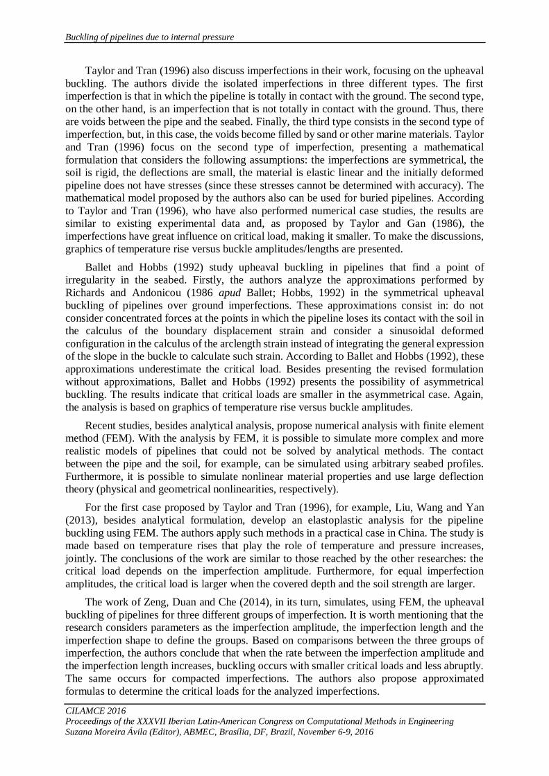
Figure 5. Post-buckling configurations – static analysis – load type a – case 2
Figure 6. Equilibrium paths (midspan) – static analysis –load type a – case 2
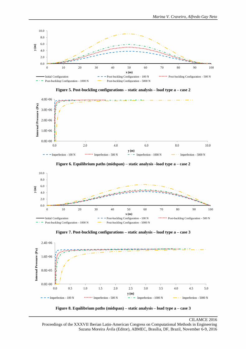
Figure 7. Post-buckling configurations – static analysis – load type a – case 3
Figure 8. Equilibrium paths (midspan) – static analysis – load type a – case 3
0.0
2.0
4.0
6.0
8.0
10.0
0 10 20 30 40 50 60 70 80 90 100
y (m
)
x (m)
Initial Configuration Post-buckling Configuration - 100 N Post-buckling Configuration - 500 N
Post-buckling Configuration - 1000 N Post-buckling Configuration - 5000 N
0.0E+00
1.0E+06
2.0E+06
3.0E+06
4.0E+06
0.0 2.0 4.0 6.0 8.0 10.0
Inte
rn
al
Press
ure (
Pa
)
y (m)
Imperfection - 100 N Imperfection - 500 N Imperfection - 1000 N Imperfection - 5000 N
0.0
2.0
4.0
6.0
8.0
10.0
0 10 20 30 40 50 60 70 80 90 100
y (m
)
x (m)
Initial Configuration Post-buckling Configuration - 100 N Post-buckling Configuration - 500 N
Post-buckling Configuration - 1000 N Post-buckling Configuration - 5000 N
0.0E+00
8.0E+05
1.6E+06
2.4E+06
0.0 0.5 1.0 1.5 2.0 2.5 3.0 3.5 4.0 4.5 5.0
Inte
rn
al
Press
ure (
Pa
)
y (m)
Imperfection - 100 N Imperfection - 500 N Imperfection - 1000 N Imperfection - 5000 N

Buckling of pipelines due to internal pressure
CILAMCE 2016 Proceedings of the XXXVII Iberian Latin-American Congress on Computational Methods in Engineering
Suzana Moreira Ávila (Editor), ABMEC, Brasília, DF, Brazil, November 6-9, 2016
Comparing the post-buckling configurations for the various imperfections (Fig. 3, Fig. 5
and Fig. 7), it can be implied that, for the cases 1 and 3, the post-buckling configuration does
not change significantly with the increase of the magnitude of the imperfections. The difference
starts to appear only for the imperfection of 5000 N in both post-buckling configurations and
equilibrium paths. In the case 2, however, the post-buckling configuration changes with
imperfections. In this case, for instance, the difference between the midspan displacements for
the imperfections of 1000 N and 5000 N almost reaches the value of one hundred percent. It
also can be verified from Fig. 3, Fig. 5 and Fig. 7 the necessity of nonlinear analyses to
determine the correct final shapes of the deflected pipelines since the displacements and
rotations are not small. It is possible to visualize, for instance, the longitudinal displacements
when these degrees of freedom allow the movement.
Analyzing the equilibrium paths (Fig. 4, Fig. 6, Fig. 8), it is important to say that the
horizontal levels that exist when the internal pressure is zero represent the deflections caused
by the imperfections. Also from the equilibrium paths, the results obtained by Taylor and Gan
(1986) can be visualized in terms of internal pressure. For small imperfections, the critical
internal pressures tend to the critical internal pressures obtained for perfect pipelines in the
small deflection theory (Table 1). If the imperfections increase, the critical internal pressures
decrease. The equilibrium paths, however, present a more smooth stiffness change along the
load increasing and the displacements do not change so abruptly.
The next stage of the numerical analysis consists in applying axial compression forces in
the pipelines corresponding to the internal pressures (Table 3). These forces are applied as
follower (load type b) and non-follower (load type c) loads. The results are obtained for the
imperfection of 1000 N and compared with the results obtained for the internal pressure load.
Figure 9. Post-buckling configurations – static analysis – load types – case 1
Figure 10. Equilibrium paths (midspan) – static analysis – load types – case 1
0
10
20
30
40
0 10 20 30 40 50 60 70 80 90 100
y (m
)
x (m)
Internal Pressure (load type a) Follower Axial Compression Force (load type b) Non-follower Axial Compression Force (load type c)
-452862
-377385
-301908
-226431
-150954
-75477
00.0E+00
2.5E+05
5.0E+05
7.5E+05
1.0E+06
1.3E+06
1.5E+06
0 5 10 15 20 25 30 35 Ax
ial C
om
press
ion
Fo
rce (
N)
Inte
rn
al
Press
ure (
Pa
)
y (m)
Internal Pressure (load type a) Follower Axial Compression Force (load type b) Non-follower Axial Compressive Force (load type c)

Marina V. Craveiro, Alfredo Gay Neto
CILAMCE 2016 Proceedings of the XXXVII Iberian Latin-American Congress on Computational Methods in Engineering
Suzana Moreira Ávila (Editor), ABMEC, Brasília, DF, Brazil, November 6-9, 2016
Figure 11. Post-buckling configurations – static analysis – load types – case 2
Figure 12. Equilibrium paths (midspan) – static analysis – load types – case 2
Figure 13. Post-buckling configurations – static analysis – load types – case 3
Figure 14. Equilibrium paths (midspan) – static analysis – load types – case 3
From Fig. 9 to Fig. 14, it is possible to conclude that the three approaches of load
application provide equivalent critical loads. However, the post-buckling configurations do not
coincide for all approaches. Only the analyses with load type a and load type b result in the
same post-buckling configurations and equilibrium paths. It happens because the internal
0
2
4
6
8
0 10 20 30 40 50 60 70 80 90 100
y (m
)
x (m)
Internal Pressure (load type a) Follower Axial Compression Force (load type b) Non-follower Axial Compression Force (load type c)
-1.81E+06
-1.21E+06
-6.04E+05
0.00E+000.0E+00
2.0E+06
4.0E+06
6.0E+06
0.0 1.0 2.0 3.0 4.0 5.0 6.0 7.0 Ax
ial C
om
press
ion
Fo
rce (
N)
Inte
rn
al
Press
ure (
Pa
)
y (m)
Internal Pressure (load type a) Follower Axial Compression Force (load type b) Non-follower Axial Compression Force (load type c)
0
5
10
15
0 10 20 30 40 50 60 70 80 90 100
y (m
)
x (m)
Internal Pressure (load type a) Follower Axial Compression Force (load type b) Non-follower Axial Compression Force (load type c)
-9.1E+05
-6.0E+05
-3.0E+05
0.0E+000.0E+00
1.0E+06
2.0E+06
3.0E+06
0 2 4 6 8 10 12 14 Ax
ial C
om
press
ion
Fo
rce (
N)
Inte
rn
al
Press
ure (
Pa
)
y (m)Internal Pressure (load type a) Follower Axial Compression Force (load type b) Non-follower Axial Compression Force (load type c)

Buckling of pipelines due to internal pressure
CILAMCE 2016 Proceedings of the XXXVII Iberian Latin-American Congress on Computational Methods in Engineering
Suzana Moreira Ávila (Editor), ABMEC, Brasília, DF, Brazil, November 6-9, 2016
pressure has a follower characteristic, depending on the deflections of the pipeline. These
deflections are not small for problems as buckling. Therefore, the direction of the equivalent
compression force has to be updated as the pipe deflects to provide the same results obtained
with the internal pressure. The only exception is the second case in which the three approaches
coincide. It occurs because both pipe ends are prevented to rotate. Thus, the follower load does
not change its direction.
The case 4 of Table 1 has not been commented yet. Trying to capture the buckling, an
internal pressure of 30 MPa is applied. This pressure is equivalent to approximately one
hundred and twenty times the critical load indicated in Table 1. Performing the static analysis,
the results obtained are shown below.
Figure 15. Post-buckling configurations – static analysis – load type a – case 4
Figure 16. Equilibrium paths (free end) – static analysis – load type a – case 4
Analyzing the results, it is possible to see that, initially, the internal pressure has an effect
that is opposite to the imperfection. It is coherent since the load nature (follower), the boundary
conditions and the deflected pipe generate a resultant that acts in the opposite sense of
imperfection. It occurs until the pipe curvature reverses, when the deflections change their
sense. This process should occur cyclically. It can be observed from the results (Fig. 15 and
Fig. 16) that if the static analysis is used to perform the simulations, the critical internal pressure
indicated in Table 1 is not identified. Although the hypothetical internal pressure applied is
much larger than critical internal pressure obtained for a perfect pipeline in the small deflection
theory, the pipe does not buckle. It occurs because the analysis method is not compatible with
the system proposed. The system analyzed is not conservative, but circulatory. Thus, the
discussions presented in Section 2.2 can be applied in this case. The correct way to analyze the
problem is to use a dynamic approach, once the simplification given by the static analysis leads
to erroneous results, as previously predicted by Ziegler (1968). Therefore, the critical load is
not that obtained from the Euler’s problem (Table 1) but that obtained from Eq. (21).
-2
0
2
0 10 20 30 40 50 60 70 80 90 100
y (m
)
x (m)
Initial Configuration Post-buckling Configuration - 100 N Post-buckling Configuration - 500 N
Post-buckling Configuration - 1000 N Post-buckling Configuration - 5000 N
0.0E+00
1.0E+07
2.0E+07
3.0E+07
-1 0 1 2 3 4 5 6
Inte
rn
al
Press
ure (
Pa
)
y (m)
Imperfection - 100 N Imperfection - 500 N Imperfection - 1000 N Imperfection - 5000 N

Marina V. Craveiro, Alfredo Gay Neto
CILAMCE 2016 Proceedings of the XXXVII Iberian Latin-American Congress on Computational Methods in Engineering
Suzana Moreira Ávila (Editor), ABMEC, Brasília, DF, Brazil, November 6-9, 2016
To perform the dynamic analysis, the load is also applied three-way (at the free end):
internal pressure (load type a), axial compression force with follower (load type b) and non-
follower (load type c) characteristics. In order to represent a quasi-static behavior, without
relevant excitation to the natural vibration of the structure, such loads are applied linearly from
zero, at the initial time, to the values indicated in Table 4, at the time that is twenty times the
structure natural period (316 s). Damping is not considered. It is also worth mentioning that
Giraffe uses an implicit method to integrate the equations of motion: the Newmark’s method.
Table 4. Load data for dynamic analyses
Case
Critical
compression force (P1) –
Eq. (21) (N)
Critical internal
pressure (picrit) – Eq. (2) with Ttw = 0 and Te
= P1 (Pa)
Loads applied separately – at time 316 s
Load type a
(Pa)
Load type b – Eq. (2)
(N)
Load type c –
Eq. (2) (N)
4 -604998 2003923 2.20x10⁶ -664196 -664196
Performing the same simulations that were made for the first three cases, the results
obtained from the dynamic analysis are shown below for the three load types. It is important to
explain that Fig. 20 has two axes of ordinates in order to separate the results obtained for load
types a and b from the results obtained for load type c, since such results are significantly
different.
Figure 17. Post-buckling configurations at time 316 s – dynamic analysis – load type a – case 4
Figure 18. Time-series of displacement (free end) – dynamic analysis – load type a – case 4
-5
-3
0
0 10 20 30 40 50 60 70 80 90 100
y (m
)
x (m)
Initial Configuration Post-buckling Configuration - 100 N Post-buckling Configuration - 500 N
Post-buckling Configuration - 1000 N Post-buckling Configuration - 5000 N
-15
-5
5
15
25
0 70 140 210 280 350
y (m
)
Time (s)
Imperfection - 100 N Imperfection - 500 N Imperfection - 1000 N Imperfection - 5000 N

Buckling of pipelines due to internal pressure
CILAMCE 2016 Proceedings of the XXXVII Iberian Latin-American Congress on Computational Methods in Engineering
Suzana Moreira Ávila (Editor), ABMEC, Brasília, DF, Brazil, November 6-9, 2016
Figure 19. Post-buckling configurations at time 316 s – dynamic analysis – load types – case 4
Figure 20. Time-series of displacement (free end) – dynamic analysis – load types – case 4
It is possible to observe from Fig. 17 and Fig. 18 that the post-buckling configurations
present significant differences for the distinct imperfections. Besides this, it can be noted that
the instability of the system is represented by crescent oscillation amplitudes (called flutter) and
the same analysis that was made for cases 1, 2 and 3 may be made again for case 4: the critical
load (obtained from the equivalent critical time of Fig. 18) for pipelines with small
imperfections tends to the critical load for perfect pipelines (Table 4). One aspect that differs
the case 4 to the other cases is the instability type. In the cases 1, 2 and 3, the instability is
characterized by the divergence whereas the instability of case 4 is characterized by the flutter.
A more accurate analysis of this difference can be done by the extraction of the eigenvalues of
the system’s state variable matrix and by the Lyapunov’s first method.
From Fig. 19 and Fig. 20, again it is observed an equivalence between the analyses
performed with internal pressure and follower axial compression force. The problem with non-
follower axial compression force presents results totally different since it represents another
phenomenon which does not characterize the internal pressure effects and could be analyzed
statically, since it represents a conservative system.
4 CONCLUSIONS
Through the literature review it was found that there are few researches about instability of
pipelines that deal exclusively with the effects of internal pressure. Based on this motivation,
the present work has discussed some theoretical aspects about effective axial force, which is
-10
0
10
20
30
40
50
-80 -60 -40 -20 0 20 40 60 80 100
y (m
)
x (m)
Internal Pressure (load type a) Follower Axial Compression Force (load type b) Non-follower Axial Compression Force (load type c)
-5
10
25
40
55
70
85
-5
5
15
0 70 140 210 280 350
y (
m)
for
loa
d t
yp
e c
y (
m)
for
loa
d t
yp
es a
an
d b
Time (s)
Internal Pressure (load type a) Follower Axial Compression Force (load type b) Non-follower Axial Compression Force (load type c)

Marina V. Craveiro, Alfredo Gay Neto
CILAMCE 2016 Proceedings of the XXXVII Iberian Latin-American Congress on Computational Methods in Engineering
Suzana Moreira Ávila (Editor), ABMEC, Brasília, DF, Brazil, November 6-9, 2016
responsible for buckling of pipelines, and about stability of structures, discussing the
applicability of static and dynamic analyses in geometrically-simple columns problems. The
concepts discussed were applied in pipelines by the performance of numerical analyses in the
software Giraffe. Three approaches were used to apply the internal pressure and to analyze its
effects: the internal pressure properly speaking and equivalent compression loads, with follower
and non-follower characteristics. Moreover, two analysis methods were employed depending
on boundary conditions and load approaches: static and dynamic analyses.
Firstly, the effect of imperfections in the instability of pipelines subjected to internal
pressure was analyzed in terms of post-buckling configurations and equilibrium paths/time-
series of displacement. In general, the conclusion, corroborating the results of previous
researches, is that, for small imperfections, the critical internal pressures tend to the critical
internal pressures obtained analytically for perfect pipelines. If the imperfections increase, the
critical internal pressures decrease. From static results, when it was applicable, it could be
observed that large imperfections, although decrease the critical load, make the equilibrium
paths more stable.
Another discussion performed was related to the equivalence between the three approaches
of application of internal pressure. The conclusion is that, applying the internal pressure as
internal pressure properly speaking or applying the internal pressure as an equivalent
compression follower axial force, the results generated are the same both for post-buckling
configurations and equilibrium paths/time-series of displacement. In the case 2, in which the
boundary conditions do not allow the rotation of the application point of the axial compression
force, the results provided by the non-follower axial force also coincide with the other two
approaches. It is worth mentioning that it is not a general result, but it is applicable for a specific
case. Further studies will address a possible generalization.
All the conclusions aforementioned discussed apply both for the results obtained from
static and dynamic analyses, if such analysis methods are employed properly. In other words,
if the analysis methods are compatible with the physical systems analyzed. In general, the static
analysis can be employed for conservative systems while the dynamic analysis can also be
employed for non-conservative systems as, for instance, circulatory systems (case 4). To
finalize, the system nature depends on the boundary conditions and the load approaches.
Acknowledgements
The first author acknowledges CNPq (Conselho Nacional de Desenvolvimento Científico
e Tecnológico) under the grant 308190/2015-7.
REFERENCES
Bai, Q., Bai, Y., 2014. Subsea pipeline design, analysis, and installation. Elsevier.
Ballet, J. P., Hobbs, R. E., 1992. Asymmetric effects of prop imperfections on the upheaval
buckling of pipelines. Thin-walled Structures, vol. 13, n. 5, pp. 355-373.
Bazant, Z. P., Cedolin, L., 2010. Stability of structures: elastic, inelastic, fracture and
damage theories. World Scientific Publishing Company.
Cardoso, C. de O., 2005. Metodologia para análise e projeto de dutos submarinos submetidos
a altas pressões e temperaturas via aplicação do método dos elementos finitos. Tese
(Doutorado), Universidade Federal do Rio de Janeiro.
Buckling of pipelines due to internal pressure
CILAMCE 2016 Proceedings of the XXXVII Iberian Latin-American Congress on Computational Methods in Engineering
Suzana Moreira Ávila (Editor), ABMEC, Brasília, DF, Brazil, November 6-9, 2016
Dvorkin, E. N., Toscano, R. G., 2001. Effects of internal/external pressure on the global
buckling of pipelines. In: First MIT Conference on Computational Fluid and Solid
Mechanics, pp. 159-164.
Fan, S., 2013. Upheaval buckling of offshore pipelines. Master thesis, Norwegian University of
Science and Technology.
Fyrileiv, O., Coolberg, L., 2005. Influence of pressure in pipeline design: effective axial force.
In: 24th International Conference on Offshore Mechanics and Arctic Engineering, pp. 1-
8.
Gay Neto, A., 2016. Dynamics of offshore risers using a geometrically-exact beam model with
hydrodynamic loads and contact with the seabed. Engineering Structures, vol. 125, pp.
438-454.
Gay Neto, A., Martins, C. de A., 2013. Structural stability of flexible lines in catenary
configuration under torsion. Marine Structures, vol. 34, pp. 16-40.
Gay Neto, A., Martins, C. de A., Pimenta, P. de M., 2016. Hydrostatic pressure load in pipes
modeled using beam finite elements: theoretical discussions and applications. Accepted by
Journal of Engineering Mechanics.
Gay Neto, A., Martins, C. de A., Pimenta, P. de M., 2014. Static analysis of offshore risers with
a geometrically-exact 3D beam model subjected to unilateral contact. Comp Mechanics,
vol. 53, pp. 125-145.
Gay Neto, A., Pimenta, P. de M., Wriggers, P., 2015. Self-contact modeling on beams
experiencing loop formation. Comp Mechanics, vol. 55, pp. 193-208.
Hobbs, R. E., 1984. In-service buckling of heated pipelines. Journal of Transportation
Engineering, vol. 110, n. 2, pp. 175-189.
Isaac, O. I., 2013. Lateral buckling and axial walking of surface laid subsea pipeline. Master
thesis, University of Stavanger.
Liu, R., Wang, W., Yan, S., 2013. Finite element analysis on thermal upheaval buckling of
submarine burial pipelines with initial imperfection. Journal of Central South University,
vol. 20, n. 1, pp. 236-245.
Sparks, C. P., 1984. The influence of tension, pressure and weight on pipe and riser
deformations and stresses. Journal of Energy Resources Technology, vol. 106, n. 1, pp. 46-
54.
Taylor, N., Gan, A. B., 1986. Submarine pipeline buckling: imperfection studies. Thin-walled
Structures, vol. 4, n. 4, pp. 295-323.
Taylor, N., Tran, V., 1996. Experimental and theoretical studies in subsea pipeline
buckling. Marine Structures, vol. 9, n. 2, pp. 211-257.
Zeng, X., Duan, M., Che, X., 2014. Critical upheaval buckling forces of imperfect
pipelines. Applied Ocean Research, vol. 45, pp. 33-39.
Ziegler, H., 1968. Principles of structural stability. Blaisdell Publishing Company.