BTRY 4090 / STSCI 4090, Spring 2010 - Rutgers...
311
Cornell University, BTRY 4090 / STSCI 4090 Spring 2010 Instructor: Ping Li 1 BTRY 4090 / STSCI 4090, Spring 2010 Theory of Statistics Instructor: Ping Li Department of Statistical Science Cornell University
Transcript of BTRY 4090 / STSCI 4090, Spring 2010 - Rutgers...

Cornell University, BTRY 4090 / STSCI 4090 Spring 2010 Instructor: Ping Li 1
BTRY 4090 / STSCI 4090, Spring 2010
Theory of Statistics
Instructor: Ping Li
Department of Statistical Science
Cornell University

Cornell University, BTRY 4090 / STSCI 4090 Spring 2010 Instructor: Ping Li 2
General Information
• Lectures: Tue, Thu 10:10-11:25 am, Stimson Hall G01
• Section: Mon 2:55 - 4:10 pm, Warren Hall 131
• Instructor: Ping Li, [email protected],
Office Hours: Tue, Thu 11:25 am -12 pm, 1192, Comstock Hall
• TA: Xiao Luo, [email protected]. Office hours: TBD
(1) Mon, 4:10 - 5:10pm Warren Hall 131;
(2) Wed, 2:30 - 3:30pm, Comstock Hall 1181.
• Prerequisites: BTRY 4080 or equivalent
• Textbook: Rice, Mathematical Statistics and Data Analysis, 3rd edition

Cornell University, BTRY 4090 / STSCI 4090 Spring 2010 Instructor: Ping Li 3
• Exams:
– Prelim 1: In Class, Feb. 25, 2010
– Prelim 2: In Class, April 8, 2010
– Final Exam: Warren Hall 145, 2pm - 4:30pm, May 13, 2010
– Policy: Close book, close notes
• Programming: Some programming assignments. You can either use Matlab
or R. For practice, please download the Matlab examples in 4080 lecture
notes.

Cornell University, BTRY 4090 / STSCI 4090 Spring 2010 Instructor: Ping Li 4
• Homework: Weekly
– Please turn in your homework either in class or to BSCB front desk
(Comstock Hall, 1198).
– No late homework will be accepted.
– Before computing your overall homework grade, the assignment with the
lowest grade (if ≥ 25%) will be dropped, the one with the second lowest
grade (if ≥ 50%) will also be dropped.
– It is the students’ responsibility to keep copies of the submitted homework.

Cornell University, BTRY 4090 / STSCI 4090 Spring 2010 Instructor: Ping Li 5
• Grading: Two formulas
1. Homework: 30% + Two Prelims: 35% + Final: 35%
2. Homework: 30% + Two Prelims: 25% + Final: 45%
Your grade is whichever higher.
• Course Letter Grade Assignment
A ≈ 90% (in the absolute scale)
C ≈ 60% (in the absolute scale)
In borderline cases, participation in section and class interactions will be used as
a determining factor.

Cornell University, BTRY 4090 / STSCI 4090 Spring 2010 Instructor: Ping Li 6
Syllabus
Topic Textbook
Random number generation
Probability, Random Variables, Joint Distributions, Expected Values Chapters 1-4
Limit Theorems Chapter 5
Distributions Derived from the Normal Distribution Chapter 6
Estimation of Parameters and Fitting of Probability Distributions Chapter 8
Testing Hypothesis and Assessing Goodness of Fit Chapter 9
Comparing Two Samples Chapter 11
The Analysis of Categorical Data Chapter 13
Linear Least Squares Chapter 14

Cornell University, BTRY 4090 / STSCI 4090 Spring 2010 Instructor: Ping Li 7
Chapters 1 to 4: Mostly Reviews
• Random number generation
• The method of random projections : A real example
of using probability to solve computationally intensive (or infeasible) problems.
• Capture/Recpature method : An example of discrete probability and
the introduction to parameter estimation using maximum likelihood.
• Conditional expectations, bivariate normal, and random pr ojections
• Moment generating function and random projections

Cornell University, BTRY 4090 / STSCI 4090 Spring 2010 Instructor: Ping Li 8
Nonuniform Sampling by Inversion
The goal : Sample X from a distribution F (x).
The inversion transform sampling :
• Sample U ∼ Uniform(0, 1).
• OutputX = F−1(U)
Proof:
Pr (X ≤ x) = Pr(
F−1(U) ≤ x)
= Pr (U ≤ F (x)) = F (x)
Limitation: Need a closed-form F−1, but many common distributions (eg,
normal) do not have closed-form F−1.

Cornell University, BTRY 4090 / STSCI 4090 Spring 2010 Instructor: Ping Li 9
Examples of Inversion Transform Sampling
• X ∼ Exponential(λ), i.e., F (x) = 1 − e−λx, x ≥ 0.
Let U ∼ Uniform(0, 1), thenlog(1−U)
−λ ∼ Exponential(λ)
• X ∼ Pareto(α), i.e., F (x) = 1 − 1xα , x ≥ 1.
Let U ∼ Uniform(0, 1), then 1(1−U)1/α ∼ Pareto(α).
A small trick:
If U ∼ Uniform(0, 1), then 1 − U ∼ Uniform(0, 1).
Thus, we can replace 1 − U by U .

Cornell University, BTRY 4090 / STSCI 4090 Spring 2010 Instructor: Ping Li 10
The Box-Muller Transform
U1 and U2 are i.i.d. samples from Uniform(0, 1). Then
N1 =√
−2 logU1 cos(2πU2)
N2 =√
−2 logU1 sin(2πU2)
are two i.i.d samples from the standard normalN(0, 1).
Q: How to generate non-standard normals?

Cornell University, BTRY 4090 / STSCI 4090 Spring 2010 Instructor: Ping Li 11
An Introduction to Random Projections
Many applications require a data matrix : A ∈ Rn×D
For example, the term-by-document matrix may contain n = 1010 documents
(web pages) andD = 106 single words, orD = 1012 double words (bi-gram
model), or D = 1018 triple words (tri-gram model).
Many matrix operations boil down to computing how close (how far) two rows
(columns) of the matrix are. For example, linear least square (ATA)−1
ATy.
Challenges : The matrix may be too large to store,
or computing ATA is too expensive.

Cornell University, BTRY 4090 / STSCI 4090 Spring 2010 Instructor: Ping Li 12
Random Projections : Replace A by B = A × R
A R = B
R ∈ RD×k: a random matrix, with i.i.d. entries sampled from N(0, 1).
B ∈ Rn×k : projected matrix, also random.
k is very small (eg k = 50 ∼ 100), but n andD are very large.
B approximately preserves the Euclidean distance and dot products between any
two rows of A. In particular,E (BBT) = AAT.

Cornell University, BTRY 4090 / STSCI 4090 Spring 2010 Instructor: Ping Li 13
Consider first two rows in A: u1, u2 ∈ RD .
u1 = u1,1, u1,2, u1,3, ..., u1,i, ..., u1,Du2 = u2,1, u2,2, u2,3, ..., u2,i, ..., u2,D
and first two rows in B: v1, v2 ∈ Rk .
v1 = v1,1, v1,2, v1,3, ..., v1,j, ..., v1,kv2 = v2,1, v2,2, v2,3, ..., v2,j, ..., v2,k
v1 = RTu1, v2 = RTu2.
R = rij, i = 1 to D and j = 1 to k. rij ∼ N(0, 1).

Cornell University, BTRY 4090 / STSCI 4090 Spring 2010 Instructor: Ping Li 14
v1 = RTu1, v2 = RTu2. R = rij, i = 1 to D and j = 1 to k.
v1,j =D∑
i=1
riju1,i, v2,j =D∑
i=1
riju2,i,
v1,j − v2,j =
D∑
i=1
rij [u1,i − u2,i]
The Euclidean norm of u1:∑D
i=1 |u1,i|2.
The Euclidean norm of v1:∑k
j=1 |v1,j |2.
The Euclidean distance between u1 and u2:∑D
i=1 |u1,i − u2,i|2.
The Euclidean distance between v1 and v2:∑k
j=1 |v1,j − v2,j |2.

Cornell University, BTRY 4090 / STSCI 4090 Spring 2010 Instructor: Ping Li 15
What are we hoping for?
•∑k
j=1 |v1,j |2 ≈∑D
i=1 |u1,i|2, as close as possible.
• ∑kj=1 |v1,j − v2,j |2 ≈∑D
i=1 |u1,i − u2,i|2, as close as possible.
• k should be as small as possible, for a specified level of accuracy.

Cornell University, BTRY 4090 / STSCI 4090 Spring 2010 Instructor: Ping Li 16
Unbiased Estimator of d and m1, m2
We need a good estimator, unbiased and has small variance.
Note that the estimation problem is essentially the same for d and for m1 (m2).
Thus, we can focus on estimating m1.
By random projections, we have k i.i..d. samples (why?)
vj =D∑
i=1
riju1,i, j = 1, 2, ...k
Because rij ∼ N(0, 1), we can develop estimators and analyze the properties
using normal and χ2 distributions. But we can also solve the problem without
using normals.

Cornell University, BTRY 4090 / STSCI 4090 Spring 2010 Instructor: Ping Li 17
Unbiased Estimator of m1
v1,j =D∑
i=1
riju1,i, j = 1, 2, ...k, (rij ∼ N(0, 1))
To get started, let’s first look the moments
E(v1,j) = E
(
D∑
i=1
riju1,i
)
=D∑
i=1
E(rij)u1,i = 0

Cornell University, BTRY 4090 / STSCI 4090 Spring 2010 Instructor: Ping Li 18
E(v21,j) =E
[
D∑
i=1
riju1,i
]2
=E
D∑
i=1
r2iju21,i +
∑
i 6=i′
riju1,iri′ju1,i′
=
D∑
i=1
E(r2ij)u21,i +
∑
i 6=i′
E(rijri′j)u1,iu1,i′
=
(
D∑
i=1
u21,i + 0
)
= m1
Great! m1 is exactly what we are after.
Since we have k, i.i.d. samples vj , we can simply average them to estimate m1.

Cornell University, BTRY 4090 / STSCI 4090 Spring 2010 Instructor: Ping Li 19
An unbiased estimator of the Euclidean norm m1 =∑D
i=1 |u1,i|2
m1 =1
k
k∑
j=1
|v1,j |2,
E (m1) =1
k
k∑
j=1
E(
|v1,j |2)
=1
k
k∑
j=1
m1 = m1
We need to analyze its variance to assess its accuracy.
Recall, our goal is to use k (number of projections) as small as possible.

Cornell University, BTRY 4090 / STSCI 4090 Spring 2010 Instructor: Ping Li 20
V ar (m1) =1
k2
k∑
j=1
V ar(
|v1,j |2)
=1
kV ar
(
|v1,j |2)
=1
k
[
E(
|v1,j |4)
−E2(|v1,j |2)]
=1
k
E
(
D∑
i=1
riju1,i
)4
−m21
We can computeE(
∑Di=1 riju1,i
)4
directly, but it would be much easier if we
take advantage of the χ2 distribution.

Cornell University, BTRY 4090 / STSCI 4090 Spring 2010 Instructor: Ping Li 21
χ2 Distribution
If X ∼ N(0, 1), then Y = X2 is a Chi-Square distribution with one degree of
freedom, denoted by χ21.
If Xj , j = 1 to k are i.i.d. normalXi ∼ N(0, 1). Then Y =∑k
j=1X2j follows
a Chi-square distribution with k degrees of freedom, denoted by χ2k.
If Y ∼ χ2k, then
E(Y ) = k, V ar(Y ) = 2k

Cornell University, BTRY 4090 / STSCI 4090 Spring 2010 Instructor: Ping Li 22
Recall, after random projections,
v1,j =D∑
i=1
riju1,i, j = 1, 2, ...k, rij ∼ N(0, 1)
Therefore, vj also has a normal distribution:
v1,j ∼ N
(
0,D∑
i=1
|ui,i|2)
= N (0, m1)
Equivalentlyv1,j√m1
∼ N(0, 1).
Therefore,
[
v1,j√m1
]2
=v21,j
m1∼ χ2
1, V ar
(
v21,j
m1
)
= 2, V ar(
v21,j
)
= 2m21
Now we can figure out the variance formula for random projections.
Cornell University, BTRY 4090 / STSCI 4090 Spring 2010 Instructor: Ping Li 23
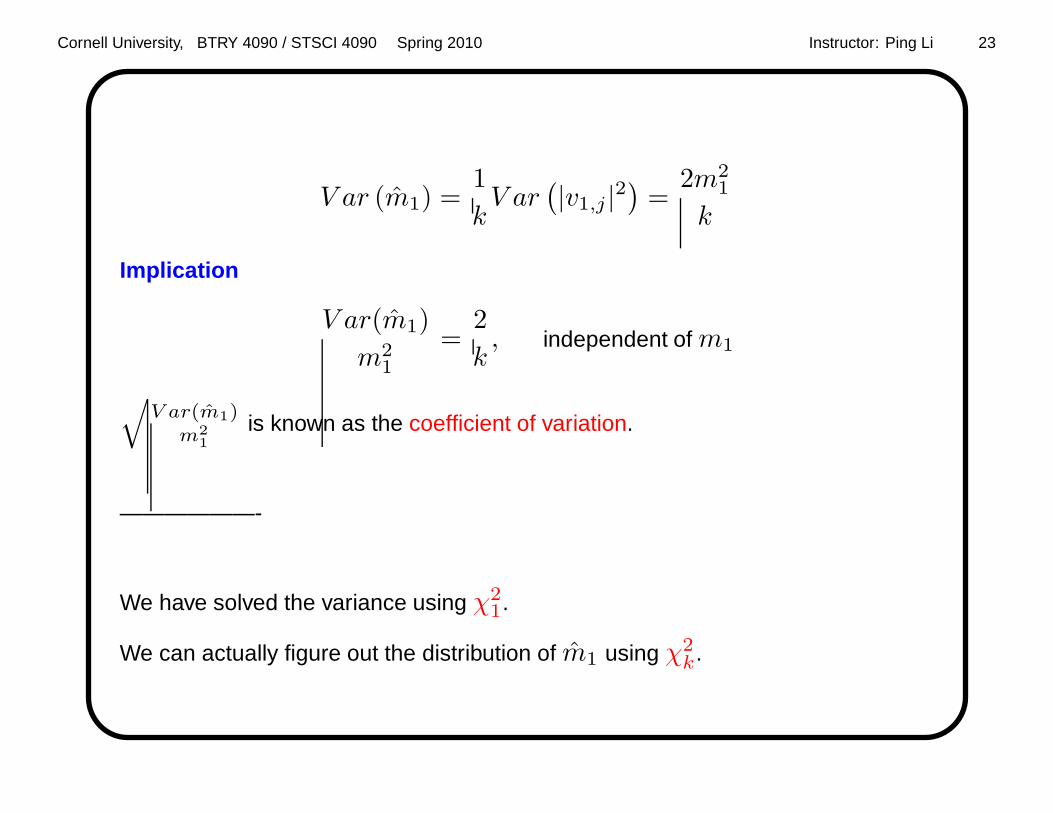
V ar (m1) =1
kV ar
(
|v1,j |2)
=2m2
1
k
Implication
V ar(m1)
m21
=2
k, independent of m1
√
V ar(m1)m2
1is known as the coefficient of variation.
——————-
We have solved the variance using χ21.
We can actually figure out the distribution of m1 using χ2k.

Cornell University, BTRY 4090 / STSCI 4090 Spring 2010 Instructor: Ping Li 24
m1 =1
k
k∑
j=1
|v1,j |2, v1,j ∼ N (0, m1)
Because v1,j ’s are i.i.d, we know
km1
m1=
k∑
j=1
(
v1,j√m1
)2
∼ χ2k (why?)
This will be useful for analyzing the error bound using probability inequalities.
We can also write down the moments of m1 directly using χ2k

Cornell University, BTRY 4090 / STSCI 4090 Spring 2010 Instructor: Ping Li 25
Recall, if Y ∼ χ2k , then E(Y ) = k, and V ar(Y ) = 2k
=⇒
E
(
km1
m1
)
= k, V ar
(
km1
m1
)
= 2k,
=⇒
V ar(m1) = 2km2
1
k2=
2m21
k

Cornell University, BTRY 4090 / STSCI 4090 Spring 2010 Instructor: Ping Li 26
An unbiased estimator of the Euclidean distance d =∑D
i=1 |u1,i − u2,i|2
d =1
k
k∑
j=1
|v1,j − v2,j |2,kd
d∼ χ2
k, V ar(d) =2d2
k.
They can be derived exactly the way as we analyze the estimator of m1.
Note that the coefficient of variation for d
V ar(d)
d2=
2
k, independent of d
meaning that the errors are pre-determined by k, a huge advantage.

Cornell University, BTRY 4090 / STSCI 4090 Spring 2010 Instructor: Ping Li 27
More probability problems
• What is the error probability P(
|d− d| ≥ ǫd)
?
• How large k should be?
• What about the inner (dot) product a =∑D
i=1 u1,iu2,i?
Cornell University, BTRY 4090 / STSCI 4090 Spring 2010 Instructor: Ping Li 28
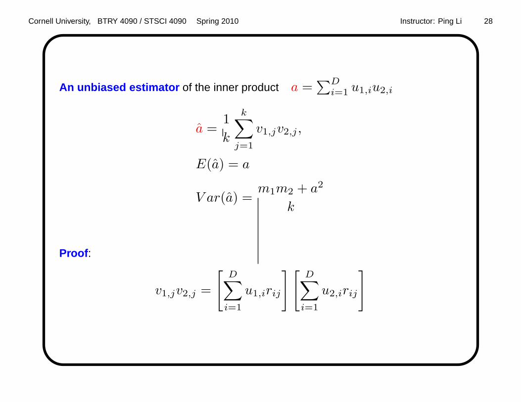
An unbiased estimator of the inner product a =∑D
i=1 u1,iu2,i
a =1
k
k∑
j=1
v1,jv2,j ,
E(a) = a
V ar(a) =m1m2 + a2
k
Proof :
v1,jv2,j =
[
D∑
i=1
u1,irij
][
D∑
i=1
u2,irij
]

Cornell University, BTRY 4090 / STSCI 4090 Spring 2010 Instructor: Ping Li 29
v1,jv2,j =
[
D∑
i=1
u1,irij
][
D∑
i=1
u2,irij
]
=D∑
i=1
u1,iu2,ir2ij +
∑
i 6=i′
u1,iu2,i′rijri′j
=⇒
E(v1,jv2,j) =D∑
i=1
u1,iu2,iE[
r2ij]
+∑
i 6=i′
u1,iu2,i′E [rijri′j ]
=D∑
i=1
u1,iu2,i1 +∑
i 6=i′
u1,iu2,i′0
=
D∑
i=1
u1,iu2,i = a
This proves the unbiasedness.

Cornell University, BTRY 4090 / STSCI 4090 Spring 2010 Instructor: Ping Li 30
We first derive the variance of a using a complicated brute force method, then we
show a much simpler method using conditional expectation.
[v1,jv2,j ]2 =
D∑
i=1
u1,iu2,ir2ij +
∑
i 6=i′
u1,iu2,i′rijri′j
2
=
[
D∑
i=1
u1,iu2,ir2ij
]2
+
∑
i 6=i′
u1,iu2,i′rijri′j
2
+ ...
=D∑
i=1
[u1,iu2,i]2 r4ij + 2
∑
i 6=i′
u1,iu2,iu1,i′u2,i′ [rijri′j ]2
+∑
i 6=i′
[u1,iu2,i′ ]2 [rijri′j ]
2 + ...
Why can we ignore the rest of the terms (after taking expectations)?

Cornell University, BTRY 4090 / STSCI 4090 Spring 2010 Instructor: Ping Li 31
Why can we ignore the rest of the terms (after taking expectations)?
Recall rij ∼ N(0, 1) i.i.d.
E(rij) = 0, E(r2ij) = 1, E(rijri′j) = E(rij)E(ri′j) = 0
E(r3ij) = 0, E(r4ij) = 3, E(r2ijri′j) = E(r2ij)E(ri′j) = 0

Cornell University, BTRY 4090 / STSCI 4090 Spring 2010 Instructor: Ping Li 32
Therefore,
E [v1,jv2,j ]2 =
D∑
i=1
3 [u1,iu2,i]2 + 2
∑
i 6=i′
u1,iu2,iu1,i′u2,i′ +∑
i 6=i′
[u1,iu2,i′ ]2
But
a2 =
[
D∑
i=1
u1,iu2,i
]2
=
D∑
i=1
[u1,iu2,i]2
+∑
i 6=i′
u1,iu2,iu1,i′u2,i′
m1m2 =
[
D∑
i=1
|u1,i|2][
D∑
i=1
|u2,i|2]
=D∑
i=1
[u1,iu2,i]2 +
∑
i 6=i′
[u1,iu2,i′ ]2
Therefore,
E [v1,jv2,j ]2 = m1m2 + 2a2, V ar [v1,jv2,j ] = m1m2 + a2

Cornell University, BTRY 4090 / STSCI 4090 Spring 2010 Instructor: Ping Li 33
An unbiased estimator of the inner product a =∑D
i=1 u1,iu2,i
a =1
k
k∑
j=1
v1,jv2,j , E(a) = a
V ar(a) =m1m2 + a2
k
The coefficient of variation
√
V ar(a)a2 =
√
m1m2+a2
a21k , not independent of a.
When two vectors u1 and u2 are almost orthogonal, a ≈ 0,
=⇒ coefficient of variation ≈ ∞.
=⇒ random projections may not be good for estimating inner products.

Cornell University, BTRY 4090 / STSCI 4090 Spring 2010 Instructor: Ping Li 34
The joint distribution of v1,j =∑D
i=1 u1,irij and v2,j =∑D
i=1 u2,irij .
E(v1,j) = 0, V ar(v1,j) =D∑
i=1
|u1,i|2 = m1
E(v2,j) = 0, V ar(v2,j) =D∑
i=1
|u2,i|2 = m2
Cov(v1,i, v2,j) = E(v1,jv2,j) − E(v1,j)E(v2,j) = a
v1,j and v2,j are jointly normal (bivariate normal).
v1,j
v2,j
∼ N
µ =
0
0
, Σ =
m1 a
a m2
(What if we know m1 and m2 exactly? For example, by one scan of data matrix.)

Cornell University, BTRY 4090 / STSCI 4090 Spring 2010 Instructor: Ping Li 35
Summary of Random Projections
Random Projections : Replace A by B = A × R
A R = B
• An elegant method, interesting probability exercise.
• Suitable for approximating Euclidean distances in massive, dense, and
heavy-tailed (some entries are excessively large) data matrices.
• It does not take advantage of data sparsity.
• We will come back to study its error probability bounds (and other things).

Cornell University, BTRY 4090 / STSCI 4090 Spring 2010 Instructor: Ping Li 36
Capture/Recapture Method: Section 1.4, Example I
The method may be used to estimate the size of a wildlife population. Suppose
that t animals are captured, tagged, and released. On a later occasion,m
animals are captured, and it is found that r of them are tagged.
Assume the total population is N .
Q 1: What is the probability mass function PN = n?
Q 2: How large is the populationN , estimated from m, r, and t ?

Cornell University, BTRY 4090 / STSCI 4090 Spring 2010 Instructor: Ping Li 37
Solution:
PN = n =
(
tr
)(
n−tm−r
)
(
nm
)
To estimate N , we can choose the N = n such that Ln = PN = n is
maximized.
Ln =
t!r!(t−r)!
(n−t)!(m−r)!(n−t−m+r)!
n!m!(n−m)!
∝(n−t)!
(n−t−m+r)!
n!(n−m)!
=(n− t)!(n−m)!
(n− t−m+ r)!n!

Cornell University, BTRY 4090 / STSCI 4090 Spring 2010 Instructor: Ping Li 38
The method of maximum likelihood To find the n such that Ln is
maximized
Ln =(n− t)!(n−m)!
(n− t−m+ r)!n!
If Ln has a global maximum, then it is equivalent to finding the n such that
gn =Ln
Ln−1= 1 =
(n− t)(n−m)
n(n− t−m+ r)
=⇒n =mt
r
Indeed, if n < mtr , then
(n− t)(n−m) − n(n− t−m+ r) = mt− nr < 0
Thus, if n < mtr , then gn is increasing; if n > mt
r , then gn is decreasing.
Cornell University, BTRY 4090 / STSCI 4090 Spring 2010 Instructor: Ping Li 39
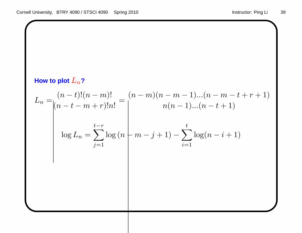
How to plot Ln?
Ln =(n− t)!(n−m)!
(n− t−m+ r)!n!=
(n−m)(n−m− 1)...(n−m− t+ r + 1)
n(n− 1)...(n− t+ 1)
logLn =t−r∑
j=1
log (n−m− j + 1) −t∑
i=1
log(n− i+ 1)

Cornell University, BTRY 4090 / STSCI 4090 Spring 2010 Instructor: Ping Li 40
20 40 60 80 100 120 140 1600
0.2
0.4
0.6
0.8
1
1.2x 10
−8
n
Like
lihoo
d
Likelihood (Ln): t = 10 m = 20 r = 4
20 40 60 80 100 120 140 1600.9
1
1.1
1.2
1.3
1.4
1.5
nLi
kelih
ood
Rat
io
Likelihood ratio (gn): t = 10 m = 20 r = 4

Cornell University, BTRY 4090 / STSCI 4090 Spring 2010 Instructor: Ping Li 41
Matlab code
function cap_recap(t, m, r);
n0 = max(t+m-r, m)+5;
j=1:(t-r); i = 1:t;
for n = n0:5 * n0
L(n-n0+1) = exp( sum(log(n-m+1-j)) - sum(log(n+1-i)));
g(n-n0+1)= (n-t) * (n-m)./n./(n-t-m+r);
end
figure;
plot(n0:5 * n0,L,’r’,’linewidth’,2);grid on;
xlabel(’n’); ylabel(’Likelihood’);
title([’Likelihood (L_n): t = ’ num2str(t) ’ m = ’ num2str(m) ’ r = ’ num2str(r)]);
figure;
plot(n0:5 * n0,g, ’r’,’linewidth’,2);grid on;
xlabel(’n’); ylabel(’Likelihood Ratio’);
title([’Likelihood ratio (g_n): t = ’ num2str(t) ’ m = ’ num2s tr(m) ’ r = ’ num2str(r)]);

Cornell University, BTRY 4090 / STSCI 4090 Spring 2010 Instructor: Ping Li 42
The Bivariate Normal Distribution
The random variables X and Y have a bivariate normal distribution if, for
constants, ux, uy , σx > 0, σy > 0, −1 < ρ < 1, their joint density function is
given, for all −∞ < x, y <∞, by
f(x, y) =1
2πσxσy
√
1 − ρ2e− 1
2(1−ρ2)
[
(x−µx)2
σ2x
+(y−µy)2
σ2y
−2ρ(x−µx)(y−µy)
σxσy
]
If X and Y are independent, then ρ = 0, and
f(x, y) =1
2πσxσye− 1
2
[
(x−µx)2
σ2x
+(y−µy)2
σ2y
]

Cornell University, BTRY 4090 / STSCI 4090 Spring 2010 Instructor: Ping Li 43
Denote that X and Y are jointly normal:
X
Y
∼ N
µ =
µx
µy
, Σ =
σ2x ρσxσy
ρσxσy σ2y
X and Y are marginally normal:
X ∼ N(µx, σ2x), Y ∼ N(µy, σ
2y)
X and Y are also conditionally normal:
X |Y ∼ N
(
µx + ρ(y − µy)σx
σy, (1 − ρ2)σ2
x
)
Y |X ∼ N
(
µy + ρ(x− µx)σy
σx, (1 − ρ2)σ2
y
)

Cornell University, BTRY 4090 / STSCI 4090 Spring 2010 Instructor: Ping Li 44
Bivariate Normal and Random Projections
A R = B
v1 and v2, the first two rows in B, have k entries:
v1,j =∑D
i=1 u1,irij and v2,j =∑D
i=1 u2,irij .
v1,j and v2,j are bivariate normal:
v1,j
v2,j
∼ N
µ =
0
0
, Σ =
m1 a
a m2
m1 =∑D
i=1 |u1,i|2, m2 =∑D
i=1 |u2,i|2, a =∑D
i=1 u1,iu2,i

Cornell University, BTRY 4090 / STSCI 4090 Spring 2010 Instructor: Ping Li 45
Simplify calculations using conditional normality
v1,j |v2,j ∼ N
(
a
m2v2,j ,
m1m2 − a2
m2
)
E (v1,jv2,j)2
=E(
E(
v21,jv
22,j |v2,j
))
= E(
v22,jE
(
v21,j |v2,j
))
=E
(
v22,j
(
m1m2 − a2
m2+
(
a
m2v2,j
)2))
=m2m1m2 − a2
m2+ 3m2
2
a2
m22
=(
m1m2 + 2a2)
.
The unbiased estimator a = 1k
∑Di=1 v1,jv2,j has variance
Var (a) =1
k
(
m1m2 + a2)

Cornell University, BTRY 4090 / STSCI 4090 Spring 2010 Instructor: Ping Li 46
Moment Generating Function (MGF)
Definition: For a random variable X , its moment generating function (MGF),
is defined as
MX(t) = E[
etX]
=
∑
x p(x)etx if X is discrete
∫∞−∞ etxf(x)dx if X is continuous
MGF MX(t) uniquely determines the distribution of X .

Cornell University, BTRY 4090 / STSCI 4090 Spring 2010 Instructor: Ping Li 47
MGF of Normal
SupposeX ∼ N(0, 1), i.e., fX(x) = 1√2πe−
−x2
2 .
MX(t) =
∫ ∞
−∞etx 1√
2πe−
x2
2 dx
=
∫ ∞
−∞
1√2πe−
x2
2 +txdx
=
∫ ∞
−∞
1√2πe−
x2−2tx+t2−t2
2 dx
=et2
2
∫ ∞
−∞
1√2πe−
(x−t)2
2 dx
=et2
2

Cornell University, BTRY 4090 / STSCI 4090 Spring 2010 Instructor: Ping Li 48
Suppose Y ∼ N(µ, σ2).
Write Y = σX + µ, where X ∼ N(0, 1).
MY (t) = E[
etY]
= E[
eµt+σtX]
= eµtE[
eσtX]
We can view σt as another t′.
MY (t) = eµtMX(σt) = eµt × eσ2t2
2 = eµt+ σ2
2 t2

Cornell University, BTRY 4090 / STSCI 4090 Spring 2010 Instructor: Ping Li 49
MGF of Chi-Square
If Xj , j = 1 to k, are i.i.d. N(0, 1), then
Y =∑k
j=1X2j ∼ χ2
k , a Chi-squared distribution with k degrees of freedom.
What is the density function? Well, since the MGF uniquely determines the
distribution, we can analyze MGF first.
By the independence of Xj ,
MY (t) = E[
eY t]
= E[
et∑k
j=1 X2j
]
=k∏
j=1
E[
etX2j
]
=(
E[
etX2j
])k

Cornell University, BTRY 4090 / STSCI 4090 Spring 2010 Instructor: Ping Li 50
E[
etX2j
]
=
∫ ∞
−∞etx2 1√
2πe−
x2
2 dx
=
∫ ∞
−∞
1√2πe−
x2
2 +tx2
dx
=
∫ ∞
−∞
1√2πe−
x2(1−2t)2 dx
=
∫ ∞
−∞
1√2πe−
x2
2σ2 dx,
(
σ2 =1
1 − 2t
)
=σ
∫ ∞
−∞
1√2πσ
e−x2
2σ2 dx = σ
=1
(1 − 2t)1/2
MY (t) =(
E[
etX2j
])k
=1
(1 − 2t)k/2, (t < 1/2)

Cornell University, BTRY 4090 / STSCI 4090 Spring 2010 Instructor: Ping Li 51
MGF for Random Projections
In random projections , the unbiased estimator d = 1k
∑kj=1 |v1,j − v2,j |2
kd
d=
k∑
j=1
|v1,j − v2,j |2d
∼ χ2k
Q: What is the MGF of d.
Solution:
Md(t) = E(
edt)
= E
(
e
[
kdd
]
[ dtk ])
=
(
1 − 2dt
k
)−k/2
where 2dt/k < 1, i.e., t < k/(2d).

Cornell University, BTRY 4090 / STSCI 4090 Spring 2010 Instructor: Ping Li 52
Moments and MGF
MX(t) = E[
etX]
=⇒M ′X(t) = E
[
XetX]
=⇒M(n)X (t) = E
[
XnetX]
Setting t = 0,
E [Xn] = M(n)X (0)

Cornell University, BTRY 4090 / STSCI 4090 Spring 2010 Instructor: Ping Li 53
Example: X ∼ χ2k . MX(t) = 1
(1−2t)k/2 .
M ′(t) =−k2
(1 − 2t)−k/2
(−2) = k (1 − 2t)−k/2−1
M ′′(t) =k
(−k2
− 1
)
(1 − 2t)−k/2−2 (−2)
=k(k + 2) (1 − 2t)−k/2−2
Therefore,
E(X) = M ′(0) = k, E(X2) = M ′′(0) = k2 + 2k
V ar(X) = (k2 + 2k) − k2 = 2k.

Cornell University, BTRY 4090 / STSCI 4090 Spring 2010 Instructor: Ping Li 54
Example: MGF and Moments of a in Random Projections
The unbiased estimator of inner product: a = 1k
∑ki=1 v1,jv2,j .
Using conditional expectation:
v1,j |v2,j ∼ N
(
a
m2v2,j ,
m1m2 − a2
m2
)
v2,j ∼ N(0,m2)
For simplicity, let
x = v1,j , y = v2,j , µ =a
m2v2,j =
a
m2y,
σ2 =m1m2 − a2
m2

Cornell University, BTRY 4090 / STSCI 4090 Spring 2010 Instructor: Ping Li 55
E (exp(v1,jv2,jt)) = E (exp(xyt)) = E (E (exp(xyt)) |y)
Using the MGF of x|y ∼ N(µ, σ2)
E (exp(xyt)|y) = eµyt+ σ2
2 (yt)2
E (E (exp(xyt)|y)) = E(
eµyt+ σ2
2 (yt)2)
µyt+σ2
2(yt)2 = y2
(
a
m2t+
σ2
2t2)
Since y ∼ N(0,m2), we known y2
m2∼ χ2
1.

Cornell University, BTRY 4090 / STSCI 4090 Spring 2010 Instructor: Ping Li 56
Using MGF of χ21, we obtain
E(
eµyt+ σ2
2 (yt)2)
= E
(
ey2
m2m2
(
am2
t+ σ2
2 t2))
=
(
1 − 2m2
(
a
m2t+
σ2
2t2))−1/2
=(
1 − 2at−(
m1m2 − a2)
t2)− 1
2 .
By independence,
Ma(t) =
(
1 − 2at
k−(
m1m2 − a2) t2
k2
)− k2
.
Now, we can use this MGF to calculate moments of a.

Cornell University, BTRY 4090 / STSCI 4090 Spring 2010 Instructor: Ping Li 57
Ma(t) =
(
1 − 2at
k−(
m1m2 − a2) t2
k2
)− k2
,
Ma(1)(t) =(−k/2)
[
(
1 − 2at
k−(
m1m2 − a2) t2
k2
)− k2−1]
×(
−2a/k −(
m1m2 − a2) 2t
k2
)
The term in [...] will not matter after letting t = 0.
Therefore,
E(a) =(
MGFa(1)(0)
)
= (−k/2)(−2a/k) = a

Cornell University, BTRY 4090 / STSCI 4090 Spring 2010 Instructor: Ping Li 58
Following a similar procedure, we can obtain
Var (a) =m1m2 + a2
k
E (a− a)3
=2a
k2
(
3m1m2 + a2)
The centered third moment measures the skewness of the distribution and can be
quite useful, for example, testing the normality.

Cornell University, BTRY 4090 / STSCI 4090 Spring 2010 Instructor: Ping Li 59
Tail Probabilities
The tail probability P (X > t) is extremely important.
For example, in random projections,
P(
|d− d| ≥ ǫd)
tells what is the probability that the difference (error) between the estimated
Euclidian distance d and the true distance d exceeds an ǫ fraction of the true
distance d.
Q: Is it just the cumulative probability function (CDF)?
Cornell University, BTRY 4090 / STSCI 4090 Spring 2010 Instructor: Ping Li 60
Tail Probability Inequalities (Bounds)
P (X > t) ≤ ???
Reasons to study tail probability bounds:
• Even if the distribution of X is known, evaluating P (X > t) often requires
numerical methods.
• Often the exact distribution of X is unknown. Instead, we may know the
moments (mean, variance, MGF, etc).
• Theoretical reasons. For example, studying how fast the error decreases.

Cornell University, BTRY 4090 / STSCI 4090 Spring 2010 Instructor: Ping Li 61
Several Tail Probability Inequalities (Bounds)
• Markov’s Inequality .
Only use the first moment. Most basic.
• Chebyshev’s Inequality .
Only use the second moment.
• Chernoff’s Inequality .
Use the MGF. Most accurate and popular among theorists.

Cornell University, BTRY 4090 / STSCI 4090 Spring 2010 Instructor: Ping Li 62
Markov’s Inequality: Theorem A in Section 4.1
If X is a random variable with P (X ≥ 0) = 1, and for which E(X) exists, then
P (X ≥ t) ≤ E(X)
t
Proof: AssumeX is continuous with probability density f(x).
E(X) =
∫ ∞
0
xf(x)dx ≥∫ ∞
t
xf(x)dx ≥∫ ∞
t
tf(x)dx = tP (X ≥ t)
See the textbook for the proof by assumingX is discrete.
Many extremely useful bounds can be obtained from Markov’s inequality.

Cornell University, BTRY 4090 / STSCI 4090 Spring 2010 Instructor: Ping Li 63
Markov’s inequality P (X ≥ t) ≤ E(X)t . If t = kE(X), then
P (X ≥ t) = P (X ≥ kE(X)) ≤ 1
k
The error decreases at the rate of 1k , which is too slow.
The original Markov’s inequality only utilizes the first moment (hence its
inaccuracy).

Cornell University, BTRY 4090 / STSCI 4090 Spring 2010 Instructor: Ping Li 64
Chebyshev’s Inequality: Theorem C in Section 4.1
Let X be a random variable with mean µ and variance σ2. Then for any t > 0,
P (|X − µ| ≥ t) ≤ σ2
t2
Proof: Let Y = (X − µ)2 = |X − µ|2, w = t2, then
P (Y ≥ w) ≤ E(Y )
w=E (X − µ)
2
w=σ2
w
Note that |X − µ|2 ≥ t2 ⇐⇒ |x− µ| ≥ t. Therefore,
P (|X − µ| ≥ t) = P(
|X − µ|2 ≥ t2)
≤ σ2
t2

Cornell University, BTRY 4090 / STSCI 4090 Spring 2010 Instructor: Ping Li 65
Chebyshev’s inequality P (|X − µ| ≥ t) ≤ σ2
t2 . If t = kσ, then
P (|X − µ| ≥ kσ) ≤ 1
k2
The error decreases at the rate of 1k2 , which is faster than 1
k .

Cornell University, BTRY 4090 / STSCI 4090 Spring 2010 Instructor: Ping Li 66
Chernoff Inequality
Ross, Proposition 8.5.2: If X is a random variable with finite MGF MX(t),
then for any ǫ > 0
P X ≥ ǫ ≤ e−tǫMX(t), for all t > 0
P X ≤ ǫ ≤ e−tǫMX(t), for all t < 0
Application: One can choose the t to minimize the upper bounds. This
usually leads to accurate probability bounds, which decrease exponentially fast.

Cornell University, BTRY 4090 / STSCI 4090 Spring 2010 Instructor: Ping Li 67
Proof: Use Markov’s Inequality.
For t > 0, becauseX > ǫ⇐⇒ etX > etǫ (monotone transformation)
P (X > ǫ) =P(
etX ≥ etǫ)
≤E[
etX]
etǫ
=e−tǫMX(t)

Cornell University, BTRY 4090 / STSCI 4090 Spring 2010 Instructor: Ping Li 68
Tail Bounds of Normal Random Variables
X ∼ N(µ, σ2). Assume µ > 0. Need to know P (|X − µ| ≥ ǫµ) ≤ ??
Chebyshev’s inequality :
P (|X − µ| ≥ ǫµ) ≤ σ2
ǫ2µ2=
1
ǫ2
[
σ2
µ2
]
The bound is not good enough, only decreasing at the rate of 1ǫ2 .

Cornell University, BTRY 4090 / STSCI 4090 Spring 2010 Instructor: Ping Li 69
Tail Bounds of Normal Using Chernoff’s Inequality
Right tail bound P (X − µ ≥ ǫµ)
For any t > 0,
P (X − µ ≥ ǫµ)
=P (X ≥ (1 + ǫ)µ)
≤e−t(1+ǫ)µMX(t)
=e−t(1+ǫ)µeµt+σ2t2/2
=e−t(1+ǫ)µ+µt+σ2t2/2
=e−tǫµ+σ2t2/2
What’s next? Since the inequality holds for any t > 0, we can choose the t to
minimize the upper bound.

Cornell University, BTRY 4090 / STSCI 4090 Spring 2010 Instructor: Ping Li 70
Right tail bound P (X − µ ≥ ǫµ)
Choose the t = t∗ to minimize g(t) = −tǫµ+ σ2t2/2.
g′(t) = −ǫµ+ σ2t = 0 =⇒ t∗ =µǫ
σ2=⇒ g(t∗) = − ǫ
2
2
µ2
σ2
Therefore,
P (X − µ ≥ ǫµ) ≤ e−ǫ2
2µ2
σ2
decreasing at the rate of e−ǫ2 .

Cornell University, BTRY 4090 / STSCI 4090 Spring 2010 Instructor: Ping Li 71
Left tail bound P (X − µ ≤ −ǫµ)
For any t < 0,
P (X − µ ≤ −ǫµ) =P (X ≤ (1 − ǫ)µ)
≤e−t(1−ǫ)µMX(t)
=e−t(1−ǫ)µeµt+σ2t2/2
=etǫµ+σ2t2/2
Choose the t = t∗ = − µǫσ2 to minimize tǫµ+ σ2t2/2. Therefore,
P (X − µ ≤ −ǫµ) ≤ e−ǫ2
2µ2
σ2

Cornell University, BTRY 4090 / STSCI 4090 Spring 2010 Instructor: Ping Li 72
Combine left and right tail bounds P (|X − µ| ≥ ǫµ)
P (|X − µ| ≥ ǫµ)
=P (X − µ ≥ ǫµ) + P (X − µ ≤ −ǫµ)
≤2e−ǫ2
2µ2
σ2

Cornell University, BTRY 4090 / STSCI 4090 Spring 2010 Instructor: Ping Li 73
Sample Size Selection Using Tail Bounds
Xi ∼ N(
µ, σ2)
, i.i.d. i = 1 to k.
An unbiased estimator of µ is µ
µ =1
k
k∑
i=1
Xi, µ ∼ N
(
µ,σ2
k
)
Choose k such that
P (|µ− µ| ≥ ǫµ) ≤ δ
———–
We already know P (|µ− µ| ≥ ǫµ) ≤ 2e− ǫ2
2µ2
σ2/k .

Cornell University, BTRY 4090 / STSCI 4090 Spring 2010 Instructor: Ping Li 74
It suffices to select the k such that
2e−ǫ2
2kµ2
σ2 ≤ δ
=⇒e−ǫ2
2kµ2
σ2 ≤ δ
2
=⇒− ǫ2
2
kµ2
σ2≤ log
(
δ
2
)
=⇒ǫ2
2
kµ2
σ2≥ − log
(
δ
2
)
=⇒k ≥[
− log
(
δ
2
)]
2
ǫ2σ2
µ2

Cornell University, BTRY 4090 / STSCI 4090 Spring 2010 Instructor: Ping Li 75
SupposeXi ∼ N(µ, σ2), i = 1 to k, i.i.d. Then µ = 1n
∑ni=1Xi is an
unbiased estimator of µ. If the sample size k satisfies
k ≥[
log
(
2
δ
)]
2
ǫ2σ2
µ2,
then with probability at least 1 − δ, the estimated µ is within a 1 ± ǫ factor of the
true µ, i.e., |µ− µ| ≤ ǫµ.

Cornell University, BTRY 4090 / STSCI 4090 Spring 2010 Instructor: Ping Li 76
What affects sample size k?
k ≥[
log
(
2
δ
)]
2
ǫ2σ2
µ2
• δ: level of significance. Lower δ → more significant → larger k.
• σ2
µ2 : noise/signal ratio. Higher σ2
µ2 → larger k.
• ǫ: accuracy. Lower ǫ→ more accurate → larger k.
• The evaluation criterion. For example, |µ− µ| ≤ ǫµ, or |µ− µ| ≤ ǫ?

Cornell University, BTRY 4090 / STSCI 4090 Spring 2010 Instructor: Ping Li 77
Exercise : In random projections, d is the unbiased estimator of the Euclidian
distance d.
• Prove the exponential tail bound:
P(
|d− d| ≥ ǫd)
≤ e???
• Determine the sample size such that
P(
|d− d| ≥ ǫd)
≤ δ

Cornell University, BTRY 4090 / STSCI 4090 Spring 2010 Instructor: Ping Li 78
Section 4.6: Approximate Methods
Suppose we know E(X) = µX , V ar(X) = σ2X . Suppose Y = g(X).
What about E(Y ), V ar(Y ) ?
In many cases, analytical solutions are not available (or too complicated).
How about Y = aX? Easy!
We knowE(Y ) = aE(X) = aµX , V ar(Y ) = a2σ2X .

Cornell University, BTRY 4090 / STSCI 4090 Spring 2010 Instructor: Ping Li 79
The Delta Method
General idea : Linear expansion of Y = g(X) aboutX = µX .
Y = g(X) = g(µX) + (X − µX)g′(µX) +1
2(X − µX)2g′′(µX) + ...
Taking expectations on both sides:
E(Y ) = g(µX) + E(X − µX)g′(µX) +1
2E(X − µX)2g′′(µX) + ...
=⇒E(Y ) ≈ g(µX) +σ2
X
2g′′(µX)
What about the variance?

Cornell University, BTRY 4090 / STSCI 4090 Spring 2010 Instructor: Ping Li 80
Use the linear approximation only:
Y = g(X) = g(µX) + (X − µX)g′(µX) + ...
V ar(Y ) ≈ [g′(µX)]2σ2
X
How good are these approximates? Depends on the nonlinearity of g(X)
about µX .

Cornell University, BTRY 4090 / STSCI 4090 Spring 2010 Instructor: Ping Li 81
Example B in Section 4.6
X ∼ U(0, 1), Y =√X . ComputeE(Y ) and V ar(Y ).
Exact Method
E(Y ) =
∫ 1
0
√xdx =
1
1/2 + 1x1/2+1
∣
∣
∣
∣
1
0
=2
3.
E(Y 2) =
∫ 1
0
xdx =1
2, V ar(Y ) =
1
2−(
2
3
)2
=1
18= 0.0556

Cornell University, BTRY 4090 / STSCI 4090 Spring 2010 Instructor: Ping Li 82
Delta Method : X ∼ U(0, 1), E(X) = 12 , V ar(X) = 1
12 .
Y = g(X) =√X . g′(X) = 1
2X−1/2,
g′′(X) = − 12
12X
−1/2−1 = − 14X
−3/2.
E(Y ) ≈√
E(X) +V ar(X)
2
[
−1
4E−3/2(X)
]
=√
1/2 +1/12
2
[
−1
4(1/2)−3/2
]
= 0.6776
V ar(Y ) ≈V ar(X)
[
1
2E−1/2(X)
]2
=1
12
[
1
2(1/2)−1/2
]2
= 0.0417

Cornell University, BTRY 4090 / STSCI 4090 Spring 2010 Instructor: Ping Li 83
Delta Method for Sign Random Projections
The projected data v1,j and v2,j are bivariate normal.
v1,j
v2,j
∼ N
µ =
0
0
, Σ =
m1 a
a m2
, j = 1, 2, ..., k
One can use a = 1k
∑kj=1 v1,jv2,j to estimate a without bias. One can also
first estimate the angle θ = cos−1(
a√m1m2
)
using
Pr (sign(v1,j) = sign(v2,j) = 1 − θ
π
then estimate a using cos(
θ)√
m1m2. Delta method can help the analysis.
(Why sign random projections?)

Cornell University, BTRY 4090 / STSCI 4090 Spring 2010 Instructor: Ping Li 84
The Delta Method for Two Variables
Z = g(X,Y ). E(X) = µX , E(Y ) = µY , V ar(X) = σ2X ,
V ar(Y ) = σ2Y , Cov(X,Y ) = σXY .
Taylor expansion of Z = g(X,Y ), about (X = µX , Y = µY ):
Z =(X − µX)∂g(µX , µY )
∂X+
1
2(X − µX)2
∂g2(µX , µY )
∂X2
+(Y − µY )∂g(µX , µY )
∂Y+
1
2(Y − µY )2
∂g2(µY , µY )
∂Y 2
+g(µX , µY ) + (X − µX)(Y − µY )∂g2(µY , µY )
∂X∂Y+ ...

Cornell University, BTRY 4090 / STSCI 4090 Spring 2010 Instructor: Ping Li 85
Taking expectations of both sides of the expansion:
E(Z) ≈g(µX , µY ) +σ2
X
2
∂g2(µX , µY )
∂X2
+σ2
Y
2
∂g2(µX , µY )
∂Y 2+ σXY
∂g2(µY , µY )
∂X∂Y
Only using linear expansion yields
V ar(Z) ≈σ2X
(
∂g(µX , µY )
∂X
)2
+ σ2Y
(
∂g(µX , µY )
∂Y
)2
+ 2σXY
(
∂g(µX , µY )
∂X
)(
∂g(µX , µY )
∂Y
)

Cornell University, BTRY 4090 / STSCI 4090 Spring 2010 Instructor: Ping Li 86
Chapter 5: Limit Theorems
X1, X2, ..., Xn are i.i.d. samples. What Happen if n→ ∞?
• The Law of Large Numbers
• The Central Limit Theorem
• The Normal Approximation

Cornell University, BTRY 4090 / STSCI 4090 Spring 2010 Instructor: Ping Li 87
The Law of Large Numbers
Theorem 5.2.A: Let X1, X2, ..., be a sequence of independent random
variables with E(Xi) = µ and V ar(Xi) = σ2. Then, for any ǫ > 0, as
n→ ∞,
P
(∣
∣
∣
∣
∣
1
n
n∑
i=1
Xi − µ
∣
∣
∣
∣
∣
> ǫ
)
→ 0
The sequence Xn is said to Converge in probability to µ.

Cornell University, BTRY 4090 / STSCI 4090 Spring 2010 Instructor: Ping Li 88
Proof: Using Chebyshev’s Inequality.
BecauseXi’s are i.i.d.,
X =1
n
n∑
i=1
Xi.
E(X) =1
n
n∑
i=1
E(Xi) =1
nnµ = µ
V ar(X) =1
n2
n∑
i=1
V ar(Xi) =1
n2nσ2 =
σ2
n
Thus, by Chebyshev’s Inequality,
P (|X − µ| ≥ ǫ) ≤ V ar(X)
ǫ2=
σ2
nǫ2→ 0

Cornell University, BTRY 4090 / STSCI 4090 Spring 2010 Instructor: Ping Li 89
100
101
102
103
104
105
106
9.2
9.4
9.6
9.8
10
10.2
10.4
10.6
10.8
n
Sam
ple
Mea
n
Normal Distribution

Cornell University, BTRY 4090 / STSCI 4090 Spring 2010 Instructor: Ping Li 90
100
101
102
103
104
105
106
9.8
10
10.2
10.4
10.6
10.8
11
n
Sam
ple
Mea
n
Gamma Distribution

Cornell University, BTRY 4090 / STSCI 4090 Spring 2010 Instructor: Ping Li 91
100
101
102
103
104
105
106
4
6
8
10
12
14
16
n
Sam
ple
Mea
n
Uniform Distribution

Cornell University, BTRY 4090 / STSCI 4090 Spring 2010 Instructor: Ping Li 92
Matlab Code
function TestLawLargeNumbers(MEAN)
N = 10ˆ6;
figure; c = [’r’,’k’,’b’];
for repeat = 1:3
X = normrnd(MEAN, 1, 1, N); % var = 1
semilogx(cumsum(X)./(1:N),c(repeat),’linewidth’,2);
grid on; hold on;
end;
xlabel(’n’); ylabel(’Sample Mean’);
title(’Normal Distribution’);
figure;
for repeat = 1:3
X = gamrnd(MEAN.ˆ2, 1./MEAN, 1, N); % var = 1
semilogx(cumsum(X)./(1:N),c(repeat),’linewidth’,2);

Cornell University, BTRY 4090 / STSCI 4090 Spring 2010 Instructor: Ping Li 93
grid on; hold on;
end;
xlabel(’n’); ylabel(’Sample Mean’);
title(’Gamma Distribution’);
figure;
for repeat = 1:3
X = rand(1, N) * MEAN* 2;
semilogx(cumsum(X)./(1:N),c(repeat),’linewidth’,2);
grid on; hold on;
end;
xlabel(’n’); ylabel(’Sample Mean’);
title(’Uniform Distribution’);

Cornell University, BTRY 4090 / STSCI 4090 Spring 2010 Instructor: Ping Li 94
Monte Carlo Integration
To calculate
I(f) =
∫ 1
0
f(x)dx, for example f(x) = e−x2/2
Numerical integration can be difficult, especially in high-dimensions.

Cornell University, BTRY 4090 / STSCI 4090 Spring 2010 Instructor: Ping Li 95
Monte Carlo integration:
Generate n i.i.d. samplesXi ∼ U(0, 1). Then by LLN
1
n
∑
f(Xi) → E(f(Xi)) =
∫ 1
0
f(x)1dx
as n→ ∞.
Advantages
• Very flexible. The interval does not have to be [0,1]. The function f(x) can
be complicated. The function can be decomposed in various ways, e.g.,
f(x) = g(x) ∗ h(x), and one can sample from other distributions.
• Straightforward in high-dimensions, double integrals, triple integrals, etc.

Cornell University, BTRY 4090 / STSCI 4090 Spring 2010 Instructor: Ping Li 96
Major disadvantage of Monte Carlo integration
LLN converges at the rate of 1√n
, from the Central Limit theorem.
Numerical integrations converges at the rate of 1n .
However, in high-dimensions, the difference becomes smaller.
Also, there are more advanced Monte Carlo techniques to achieve better rates.

Cornell University, BTRY 4090 / STSCI 4090 Spring 2010 Instructor: Ping Li 97
Examples for Monte Carlo Numerical Integration
Treat∫ 1
0cosxdx as an expectation:
∫ 1
0
cosxdx =
∫ 1
0
1 × cosxdx = E(cos(x)), x ∼ Uniform U(0, 1)
Monte Carlo integration procedure:
• GenerateN i.i.d. samples xi ∼ Uniform U(0, 1), i = 1 to N .
• Use empirical expectation 1N
∑Ni=1 cos(xi) to approximate E(cos(x)).

Cornell University, BTRY 4090 / STSCI 4090 Spring 2010 Instructor: Ping Li 98
True value:∫ 1
0cosxdx = sin(1) = 0.8415
101
102
103
104
105
106
107
0.8
0.82
0.84
0.86
0.88
N

Cornell University, BTRY 4090 / STSCI 4090 Spring 2010 Instructor: Ping Li 99
∫ 1
0
log2(x+ 0.1)√
sin(x+ 0.1)e−x0.15
dx
101
102
103
104
105
106
107
0.5
1
1.5
2
N

Cornell University, BTRY 4090 / STSCI 4090 Spring 2010 Instructor: Ping Li 100
Section 5.3: Central Limit Theorem and Normal Approximatio n
Central Limit Theorem LetX1, X2, ..., be a sequence of independent and
identically distributed random variables, each having finite meanE(Xi) = µ and
variance σ2. Then as n→ ∞
P
X1 +X2 + ...+Xn − nµ√nσ
≤ y
→∫ y
−∞
1√2πe−
t2
2 dt

Cornell University, BTRY 4090 / STSCI 4090 Spring 2010 Instructor: Ping Li 101
Normal Approximation
X1 +X2 + ...+Xn − nµ√nσ
=X − µ√
σ2/nis approximately N(0, 1)
Non-rigorously, we may say X is approximatelyN(
µ, σ2
n
)
.
But we know E(X) = µ, V ar(X) = σ2
n .

Cornell University, BTRY 4090 / STSCI 4090 Spring 2010 Instructor: Ping Li 102
Normal Distribution Approximates Binomial
SupposeX ∼ Binomial(n, p). For fixed p, as n→ ∞
Binomial(n, p) ≈ N(µ, σ2),
µ = np, σ2 = np(1 − p).

Cornell University, BTRY 4090 / STSCI 4090 Spring 2010 Instructor: Ping Li 103
0 1 2 3 4 5 6 7 8 9 100
0.05
0.1
0.15
0.2
0.25
0.3
0.35
x
Den
sity
(m
ass)
func
tion
n = 10 p = 0.2

Cornell University, BTRY 4090 / STSCI 4090 Spring 2010 Instructor: Ping Li 104
−10 −5 0 5 10 15 20 250
0.05
0.1
0.15
0.2
0.25
x
Den
sity
(m
ass)
func
tion
n = 20 p = 0.2

Cornell University, BTRY 4090 / STSCI 4090 Spring 2010 Instructor: Ping Li 105
−10 −5 0 5 10 15 20 25 300
0.02
0.04
0.06
0.08
0.1
0.12
0.14
0.16
x
Den
sity
(m
ass)
func
tion
n = 50 p = 0.2

Cornell University, BTRY 4090 / STSCI 4090 Spring 2010 Instructor: Ping Li 106
−10 0 10 20 30 40 500
0.01
0.02
0.03
0.04
0.05
0.06
0.07
0.08
0.09
0.1
x
Den
sity
(m
ass)
func
tion
n = 100 p = 0.2

Cornell University, BTRY 4090 / STSCI 4090 Spring 2010 Instructor: Ping Li 107
100 150 200 250 3000
0.005
0.01
0.015
0.02
0.025
0.03
0.035
x
Den
sity
(m
ass)
func
tion
n = 1000 p = 0.2

Cornell University, BTRY 4090 / STSCI 4090 Spring 2010 Instructor: Ping Li 108
Matlab code
function NormalApprBinomial(n,p);
mu = n* p; sigma2 = n * p* (1-p);
figure;
bar((0:n),binopdf(0:n,n,p),’g’);hold on; grid on;
x = mu - 3 * sigma2:0.001:mu+3 * sigma2;
plot(x,normpdf(x,mu,sqrt(sigma2)),’r-’,’linewidth’, 2);
xlabel(’x’);ylabel(’Density (mass) function’);
title([’n = ’ num2str(n) ’ p = ’ num2str(p)]);

Cornell University, BTRY 4090 / STSCI 4090 Spring 2010 Instructor: Ping Li 109
Convergence in Distribution
Definition: Let X1, X2, ..., be a sequence of random variables with
cumulative distributions F1, F2, ..., and let X be a random variable with
distribution function F . We say that Xn converges in distribution to X if
limn→∞
Fn(x) = F (x)
at every point x at which F is continuous.

Cornell University, BTRY 4090 / STSCI 4090 Spring 2010 Instructor: Ping Li 110
Theorem 5.3A: Continuity Theorem
Let Fn be a sequence of cumulative distribution functions with the corresponding
MGF Mn. Let F be a cumulative distribution function with MGF M .
If Mn(t) →M(t) for all t in an open interval containing zero,
then Fn(x) → F (x) at all continuity points of F .

Cornell University, BTRY 4090 / STSCI 4090 Spring 2010 Instructor: Ping Li 111
Approximate Poisson by Normal
If X ∼ Poi(λ) is approximately normal when λ is large.
Recall Poi(λ) approximatesBin(n, p) with λ ≈ np, and large n.
——————————-
Let Xn ∼ Poi(λn). Let λ1, λ2, ... be an increasing sequence with λn → ∞.
Let Zn = Xn−λn√λn
, with CDF Fn.
Let Z ∼ N(0, 1), with CDF F .
To show Fn → F , suffices to show MZn(t) →MZ(t) = et2/2.

Cornell University, BTRY 4090 / STSCI 4090 Spring 2010 Instructor: Ping Li 112
Proof:
If Y ∼ Poi(λ), then MY (t) = eλ(et−1). Then, for Zn = Xn−λn√λn
,
MZn(t) =e− λn√
λnteλn
(
et/√
λn−1)
= exp[
−t√
λn + λn
(
et/√
λn−1)]
= exp[g(t, n)]

Cornell University, BTRY 4090 / STSCI 4090 Spring 2010 Instructor: Ping Li 113
Recall et = 1 + t+ t2
2 + t2
6 + ...
g(t, n) = − t√
λn + λn
(
et/√
λn − 1)
= − t√
λn + λn
(
t√λn
+1
2
t2
λn+
1
6
t3
λ3/2n
+ ...
)
=t2
2+
1
6
t3
λ1/2n
+ ...→ t2
2
Therefore,MZn(t) → et2/2 = MZ(t)

Cornell University, BTRY 4090 / STSCI 4090 Spring 2010 Instructor: Ping Li 114
The Proof of Central Limit Theorem
Theorem 5.3.B: Let X1, X2, ..., be a sequence of independent random
variables having mean µ and variance σ2 and the common probability distribution
function F and MGF M defined in the neighborhood of zero. Then
limn→∞
P
(∑ni=1Xi − nµ
σ√n
≤ x
)
=
∫ x
−∞
1√2πe−z2/2dz, −∞ < x <∞
Proof: Let Sn =∑n
i=1Xi and Zn = Sn−nµσ√
n. It suffices to show
MZn(t) → et2/2, as n→ ∞.

Cornell University, BTRY 4090 / STSCI 4090 Spring 2010 Instructor: Ping Li 115
Note that MSn(t) = Mn(t). Hence
MZn(t) =e− nµ
σ√
ntMSn
(
t
σ√n
)
= e−√
nµσ tMn
(
t
σ√n
)
Taylor expandM(t) about zero
M(t) =1 + tM ′(0) +t2
2M ′′(0) + ...
=1 + tµ+t2
2
(
σ2 + µ2)
+ ...

Cornell University, BTRY 4090 / STSCI 4090 Spring 2010 Instructor: Ping Li 116
Therefore,
MZn(t) =e−√
nµσ tMn
(
t
σ√n
)
=e−√
nµσ t
(
1 +µt
σ√n
+t2
2σ2n
(
σ2 + µ2)
+ ...
)n
=exp
(
−√nµ
σt+ n log
(
1 +µt
σ√n
+t2
2σ2n
(
σ2 + µ2)
+ ...
))

Cornell University, BTRY 4090 / STSCI 4090 Spring 2010 Instructor: Ping Li 117
By Taylor expansion, log(1 + x) = x− x2
2 + .... Therefore,
n log
(
1 +µt
σ√n
+t2
2σ2n
(
σ2 + µ2)
)
=n
[
µt
σ√n
+t2
2σ2n
(
σ2 + µ2)
− 1
2
(
µt
σ√n
)2
+ ...
]
=n
[
µt
σ√n
+t2
2n+ ...
]
Hence
MZn(t) = exp
(
−√nµ
σt+ n log
(
1 +µt
σ√n
+t2
2σ2n
(
σ2 + µ2)
+ ...
))
→et2/2
The textbook assumed µ = 0 to start with, which simplified the algebra.

Cornell University, BTRY 4090 / STSCI 4090 Spring 2010 Instructor: Ping Li 118
Chapter 6: Distributions Derived From Normal
• χ2 distribution If X1, X2, ..., Xn are i.i.d. N(0, 1). Then∑n
i=1X2i ∼ χ2
n, the χ2 distribution with n degrees of freedom.
• t distribution If U ∼ χ2n, Z ∼ N(0, 1), and Z and U are
independent, then Z√U/n
∼ tn, the t distribution with n degrees of freedom.
• F distribution If U ∼ χ2m, V ∼ χ2
n, and U and V are independent,
thenU/mV/n ∼ Fm,n, the F distribution with m and n degrees of freedom.

Cornell University, BTRY 4090 / STSCI 4090 Spring 2010 Instructor: Ping Li 119
χ2 Distribution
If X1, X2, ..., Xn are i.i.d. N(0, 1). Then∑n
i=1X2i ∼ χ2
n, the χ2 distribution
with n degrees of freedom.
• Z ∼ χ2n, then MGF MZ(t) = (1 − 2t)−n/2.
• Z ∼ χ2n, then E(Z) = n, V ar(Z) = 2n.
• Z1 ∼ χ2n, Z2 ∼ χ2
m, Z1 and Z2 are independent. Then
Z = Z1 + Z2 ∼ χ2n+m.
• χ2n = Gamma
(
α = n2 , λ = 1
2
)
.

Cornell University, BTRY 4090 / STSCI 4090 Spring 2010 Instructor: Ping Li 120
If X ∼ Gamma(α, λ), then MX(t) =(
λλ−t
)α
=(
11−t/λ
)α
.
If Z ∼ χ2n, then MZ(t) = (1 − 2t)
−n/2=(
11−2t
)n/2
Therefore, Z ∼ χ2n = Gamma
(
n2 ,
12
)
Therefore, the density function of Z ∼ χ2n
fZ(z) =1
2n/2Γ(n/2)zn/2−1e−z/2, z ≥ 0

Cornell University, BTRY 4090 / STSCI 4090 Spring 2010 Instructor: Ping Li 121
t Distribution
If U ∼ χ2n, Z ∼ N(0, 1), and Z and U are independent, then Z√
U/n∼ tn,
the t distribution with n degrees of freedom.
Theorem 6.2.A : The density function of the Z ∼ tn is
fZ(z) =Γ[(n+ 1)/2]√nπΓ(n/2)
(
1 +z2
n
)−(n+1)/2

Cornell University, BTRY 4090 / STSCI 4090 Spring 2010 Instructor: Ping Li 122
−5 0 50
0.05
0.1
0.15
0.2
0.25
0.3
0.35
0.4
x
dens
ity
1 degree10 degreesnormal

Cornell University, BTRY 4090 / STSCI 4090 Spring 2010 Instructor: Ping Li 123
Matlab Code
function plot_tdensity
figure;
x=-5:0.01:5;
plot(x,tpdf(x,1),’g-’,’linewidth’,2);hold on; grid on;
plot(x,tpdf(x,10),’k-’,’linewidth’,2);hold on; grid on ;
plot(x,normpdf(x),’r’,’linewidth’,2);
for n = 2:9;
plot(x,tpdf(x,n));hold on; grid on;
end;
xlabel(’x’); ylabel(’density’);
legend(’1 degree’,’10 degrees’,’normal’);

Cornell University, BTRY 4090 / STSCI 4090 Spring 2010 Instructor: Ping Li 124
Things to know about tn distributions:
• It is widely used in statistical testing, the t-test.
• It is practically indistinguishable from normal, when n ≥ 45.
• It is a heavy-tailed distribution, only has < nth moments.
• It is the Cauchy distribution when n = 1.

Cornell University, BTRY 4090 / STSCI 4090 Spring 2010 Instructor: Ping Li 125
The F Distribution
If U ∼ χ2m, V ∼ χ2
n, and U and V are independent, then
Z = U/mV/n ∼ Fm,n, the F distribution with m and n degrees of freedom.
Proposition 6.2.B: If Z ∼ Fm,n, then the density
fZ(z) =Γ[(m+ n)/2]
Γ(m/2)Γ(n/2)
(m
n
)m/2
zm/2−1(
1 +m
nz)−(m+n)/2
The F distribution is also widely used in statistical testing, the F -test.

Cornell University, BTRY 4090 / STSCI 4090 Spring 2010 Instructor: Ping Li 126
The Cauchy Distribution
If X ∼ N(0, 1) and Y ∼ N(0, 1), and X and Y are independent. Then
Z = XY has the standard Cauchy distribution, with density
fZ(z) =1
π(z2 + 1), −∞ < z <∞
Cauchy distribution does not have a finite mean,E(Z) = ∞.
It is also the t-distribution with 1 degree of freedom.

Cornell University, BTRY 4090 / STSCI 4090 Spring 2010 Instructor: Ping Li 127
Proof:
FZ(z) = P (Z ≤ z) = P
(
X
Y≤ z
)
=P (X ≤ Y z, Y > 0) + P (X ≥ Y z, Y < 0)
=2P (x ≤ yz, Y > 0)
=2
∫ ∞
0
∫ yz
0
fX,Y (x, y)dxdy
=2
∫ ∞
0
∫ yz
0
1√2πe−
x2
21√2πe−
y2
2 dxdy
=1
π
∫ ∞
0
e−y2
2
∫ yz
0
e−x2
2 dxdy
Now what? It actually appears easier to work the PDF fZ(z).

Cornell University, BTRY 4090 / STSCI 4090 Spring 2010 Instructor: Ping Li 128
Use the fact
∂∫ g(x)
ch(y)dy
∂x= h(g(x))g′(x), for any constant c.
fZ(z) =1
π
∫ ∞
0
e−y2
2
[
ye−y2z2
2
]
dy
=1
π
∫ ∞
0
e−y2(z2+1)
2 d
[
y2
2
]
=1
π
1
z2 + 1.
What’s the problem when working directly with the CDF?

Cornell University, BTRY 4090 / STSCI 4090 Spring 2010 Instructor: Ping Li 129
FZ(z) =1
π
∫ ∞
0
e−y2
2
∫ yz
0
e−x2
2 dxdy
=1
π
∫ ∞
0
∫ yz
0
e−x2+y2
2 dxdy
=1
π
∫ ∞
0
∫ π/2
tan−1(1/z)
e−r2
2 rdθdr
=1
π
∫ ∞
0
e−r2
2 r[π
2− tan−1(1/z)
]
dr
=π/2 − tan−1(1/z)
π
∫ ∞
0
e−r2
2 d
[
r2
2
]
=π/2 − tan−1(1/z)
π
Therefore,
fZ(z) =1
π
1
z2 + 1.

Cornell University, BTRY 4090 / STSCI 4090 Spring 2010 Instructor: Ping Li 130
Section 6.3: Sample Mean and Sample Variance
Let X1, X2, ..., Xn be independent samples from N(µ, σ2).
The sample mean X =1
n
n∑
i=1
Xi
The sample variance S2 =1
n− 1
n∑
i=1
(
Xi − X)2

Cornell University, BTRY 4090 / STSCI 4090 Spring 2010 Instructor: Ping Li 131
Theorem 6.3.A: The random variable X and the vector
(X1 − X, X2 − X, ..., Xn − X) are independent.
Proof: Read the book for a more rigorous proof.
Let’s only prove that X and Xi − X are uncorrelated (homework problem).

Cornell University, BTRY 4090 / STSCI 4090 Spring 2010 Instructor: Ping Li 132
Corollary 6.3.A: X and S2 are independently distributed.
Proof: It follows immediately because S2 is a function of
(X1 − X, X2 − X, ..., Xn − X).

Cornell University, BTRY 4090 / STSCI 4090 Spring 2010 Instructor: Ping Li 133
Joint Distribution of the Sample Mean and Sample Variance
Theorem 6.3.B: (n− 1)S2/σ2 ∼ χ2n−1.
Proof:
X1, X2, ..., Xn, are independent normal variables,Xi ∼ N(µ, σ2).
Intuitively, S2 = 1n−1
∑ni=1
(
Xi − X)2
should be closely related to a
Chi-squared distribution.

Cornell University, BTRY 4090 / STSCI 4090 Spring 2010 Instructor: Ping Li 134
(n− 1)S2 =
n∑
i=1
(
Xi − X)2
=n∑
i=1
(
Xi − µ+ µ− X)2
=n∑
i=1
(Xi − µ)2 − n(
µ− X)2

Cornell University, BTRY 4090 / STSCI 4090 Spring 2010 Instructor: Ping Li 135
n∑
i=1
(
Xi − µ
σ
)2
∼ χ2n
(
µ− X
σ/√n
)2
∼ χ21
Y =(n− 1)S2
σ2=
n∑
i=1
(
Xi − µ
σ
)2
−(
µ− X
σ/√n
)2
Y +
(
µ− X
σ/√n
)2
=n∑
i=1
(
Xi − µ
σ
)2
The MGFs in both sides should be equal.
Also, note that Y and X are independent.

Cornell University, BTRY 4090 / STSCI 4090 Spring 2010 Instructor: Ping Li 136
Y =(n− 1)S2
σ2, Y +
(
µ− X
σ/√n
)2
=
n∑
i=1
(
Xi − µ
σ
)2
Equating the MGFs of both sides (also using independence).
E[
etY]
(1 − 2t)−1/2 = (1 − 2t)−n/2
=⇒E[
etY]
= (1 − 2t)−(n−1)/2
Therefore,
(n− 1)S2
σ2∼ χ2
n−1

Cornell University, BTRY 4090 / STSCI 4090 Spring 2010 Instructor: Ping Li 137
Corollary 6.3.B:
X − µ
S/√n
∼ tn−1.
Proof:
X − µ
S/√n
=
X−µσ/
√n
√
(n− 1)S2/σ2/(n− 1)=
U√V
U ∼ N(0, 1). V ∼ χ2n−1. Therefore, U√
V∼ tn−1 by definition.

Cornell University, BTRY 4090 / STSCI 4090 Spring 2010 Instructor: Ping Li 138
Chapter 8: Parameter Estimation
One of the most important chapters for 4090!
Assume n i.i.d. observationsXi, i = 1 to n. Xi’s has density function with k
parameters θ1, θ2, ... ,θk , written as fX(x; θ1, θ2, ..., θk).
The task is to estimate θ1, θ2, ..., θk , from n samplesX1, X2, ..., Xn.
———————————-
Where did the density function fX come from in the first place?
This is often a chicken-egg problem, but it is not a major concern for this class.

Cornell University, BTRY 4090 / STSCI 4090 Spring 2010 Instructor: Ping Li 139
Two Basic Estimation Methods
SupposeX1, X2, ..., Xn are i.i.d. samples with density fX(x; θ1, θ2).
• The method of moments
Force 1n
∑ni=1Xi = E(X) and 1
n
∑ni=1X
2i = E(X2)
Two equations, two unknowns (θ1, θ2).
• The method of maximum likelihood
Find the θ1 and θ2 that maximizes the joint probability (likelihood)∏n
i=1 fX(xi; θ1, θ2). An optimization problem, maybe convex.

Cornell University, BTRY 4090 / STSCI 4090 Spring 2010 Instructor: Ping Li 140
The Method of Moments
Assume n i.i.d. observationsXi, i = 1 to n. Xi’s has density function with k
parameters θ1, θ2, ... ,θk , written as fX(x; θ1, θ2, ..., θk).
Define the mth theoretical moment of X
µm = E(Xm)
Define the mth empirical moment of X
µm =1
n
n∑
i=1
Xmi
Solve a system of k equations: µm = µm , m = 1 to k.
What could be the difficulties?

Cornell University, BTRY 4090 / STSCI 4090 Spring 2010 Instructor: Ping Li 141
Example 8.4.A: Xi ∼ Poisson(λ), i.i.d. i = 1 to n.
BecauseE(Xi) = λ, the moment estimator would be
λ =1
n
n∑
i=1
Xi = X
—————
Properties of λ
E(λ) =1
n
n∑
i=1
E(Xi) = λ
V ar(λ) =1
nV ar(Xi) =
λ
n

Cornell University, BTRY 4090 / STSCI 4090 Spring 2010 Instructor: Ping Li 142
Xi ∼ Poisson(λ), i.i.d. i = 1 to n.
Because V ar(Xi) = λ, we can also estimate λ by
λ2 =1
n
n∑
i=1
X2i −
(
1
n
n∑
i=1
Xi
)2
This estimator λ2 is no longer unbiased, because
E(λ2) =[
λ+ λ2]
−[
λ
n+ λ2
]
= λ− λ
n
Moment estimators are in general biased .
Q: How to modify λ2 to obtain an unbiased estimator?

Cornell University, BTRY 4090 / STSCI 4090 Spring 2010 Instructor: Ping Li 143
Example 8.4.B: Xi ∼ N(µ, σ2), i.i.d. i = 1 to n.
Solve for µ and σ2 from the equations
µ =1
n
n∑
i=1
Xi, σ2 =1
n
n∑
i=1
X2i −
(
1
n
n∑
i=1
Xi
)2
The moment estimators are
µ = X, σ2 =1
n
n∑
i=1
(Xi − X)2
We have known that µ and σ2 are independent, and
µ ∼ N
(
µ,σ2
n
)
,nσ2
σ2∼ χ2
n−1

Cornell University, BTRY 4090 / STSCI 4090 Spring 2010 Instructor: Ping Li 144
Example 8.4.C: Xi ∼ Gamma(α, λ), i.i.d. i = 1 to n.
The first two moments are
µ1 =α
λ, µ2 =
α(α+ 1)
λ2
Equivalently
α =µ2
1
µ2 − µ21
, λ =µ1
µ2 − µ21
The moment estimators are
α =µ2
1
µ2 − µ21
=X2
σ2,
λ =µ1
µ2 − µ21
=X
σ2

Cornell University, BTRY 4090 / STSCI 4090 Spring 2010 Instructor: Ping Li 145
Example 8.4.D: Assume that the random variable X has density
fX(x) =1 + αx
2, |x| ≤ 1, |α| ≤ 1
Then α can be estimated from the first moment
µ1 =
∫ 1
−1
x1 + αx
2dx =
α
3.
Therefore, the moment estimator would be
α = 3X.

Cornell University, BTRY 4090 / STSCI 4090 Spring 2010 Instructor: Ping Li 146
Consistency of Moment Estimators
Definition: Let θn be an estimator of a parameter θ based on a sample of
size n. Then θn is consistent in probability , if for any ǫ > 0,
P(
|θn − θ| ≥ ǫ)
→ 0, as n→ ∞
Moment estimators are consistent if the conditions for Weak Law of Large
Numbers are satisfied.

Cornell University, BTRY 4090 / STSCI 4090 Spring 2010 Instructor: Ping Li 147
A Simulation Study for Estimating Gamma Parameters
Consider a gamma distribution Gamma(α, λ) with α = 4 and λ = 0.5.
Generate n, for n = 5 to n = 105, samples from Gamma(α = 4, λ = 0.5).
Estimate α and λ by moment estimators for every n.
Repeat the experiment 4 times.

Cornell University, BTRY 4090 / STSCI 4090 Spring 2010 Instructor: Ping Li 148
100
101
102
103
104
105
1
1.5
2
2.5
3
3.5
4
4.5
5
5.5
6Gamma: Moment estimate of α = 4

Cornell University, BTRY 4090 / STSCI 4090 Spring 2010 Instructor: Ping Li 149
100
101
102
103
104
105
0.1
0.2
0.3
0.4
0.5
0.6
0.7
0.8
0.9Gamma: Moment estimate of λ = 0.5

Cornell University, BTRY 4090 / STSCI 4090 Spring 2010 Instructor: Ping Li 150
Matlab Code
function est_gamma
n = 10ˆ5; al =4; lam = 0.5; c = [’b’,’k’,’r’,’g’];
for t = 1:4;
X = gamrnd(al,1/lam,n,1);
mu1 = cumsum(X)./(1:n)’;
mu2 = cumsum(X.ˆ2)./(1:n)’;
est_al = mu1.ˆ2./(mu2-mu1.ˆ2);
est_lam = mu1./(mu2-mu1.ˆ2);
st =5;
figure(1);
semilogx((st:n)’,est_al(st:end),c(t), ’linewidth’,2) ; hold on; grid on;
title([’Gamma: Moment estimate of \alpha = ’ num2str(al)]) ;
figure(2);
semilogx((st:n)’,est_lam(st:end),c(t),’linewidth’,2 ); hold on; grid on;
title([’Gamma: Moment estimate of \lambda = ’ num2str(lam) ]);
end;

Cornell University, BTRY 4090 / STSCI 4090 Spring 2010 Instructor: Ping Li 151
The Method of Maximum Likelihood
Suppose that random variables X1, X2, ..., Xn have a joint density
f(x1, x2, ..., xn|θ). Given observed values Xi = xi, where i = 1 to n, the
likelihood of θ as a function of (x1, x2, .., xn) is defined as
lik(θ) = f(x1, x2, ..., xn|θ)
The method of maximum likelihood seeks the θ that maximizes lik(θ).

Cornell University, BTRY 4090 / STSCI 4090 Spring 2010 Instructor: Ping Li 152
The Log Likelihood in the I.I.D. Case
If Xi’s are i.i.d., then
lik(θ) =n∏
i=1
f(Xi|θ)
It is often more convenient to work with its logarithm, called the Log Likelihood
l(θ) =n∑
i=1
log f(Xi|θ)

Cornell University, BTRY 4090 / STSCI 4090 Spring 2010 Instructor: Ping Li 153
Example 8.5.A: SupposeX1, X2, ..., Xn, are i.i.d. samples of
Poisson(λ). Then the likelihood of λ is
lik(λ) =
n∏
i=1
λXie−λ
Xi!
The log likelihood is
l(λ) =n∑
i=1
[Xi log λ− λ− logXi!]
= log λn∑
i=1
Xi − nλ+
[
−n∑
i=1
logXi!
]
The part in [...] is useless for finding the MLE.

Cornell University, BTRY 4090 / STSCI 4090 Spring 2010 Instructor: Ping Li 154
The log likelihood is
l(λ) = log λn∑
i=1
Xi − nλ−n∑
i=1
logXi!
The MLE is the solution to l′(λ) = 0, where
l′(λ) =1
λ
n∑
i=1
Xi − n
Therefore, the MLE is λ = X , same as the moment estimator.
For verification, check l′′(λ) = − 1λ2
∑ni=1Xi≤ 0, meaning that l(λ) is a
concave function and the solution to l′(λ) = 0 is indeed the maximum.

Cornell University, BTRY 4090 / STSCI 4090 Spring 2010 Instructor: Ping Li 155
Example 8.5.B: Given n i.i.d. samples,Xi ∼ N(µ, σ2), i = 1 to n. The
log likelihood is
l(
µ, σ2)
=n∑
i=1
log fX(Xi;µ, σ2)
= − 1
2σ2
n∑
i=1
(Xi − µ)2 − 1
2n log(2πσ2)
∂l
∂µ=
1
2σ22
n∑
i=1
(Xi − µ) = 0 =⇒ µ =1
n
n∑
i=1
Xi
∂l
∂σ2=
1
2σ4
n∑
i=1
(Xi − µ)2 − n
2σ2= 0 =⇒ σ2 =
1
n
n∑
i=1
(Xi − µ)2.
Cornell University, BTRY 4090 / STSCI 4090 Spring 2010 Instructor: Ping Li 156
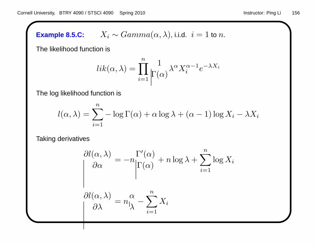
Example 8.5.C: Xi ∼ Gamma(α, λ), i.i.d. i = 1 to n.
The likelihood function is
lik(α, λ) =n∏
i=1
1
Γ(α)λαXα−1
i e−λXi
The log likelihood function is
l(α, λ) =n∑
i=1
− log Γ(α) + α log λ+ (α− 1) logXi − λXi
Taking derivatives
∂l(α, λ)
∂α= −nΓ′(α)
Γ(α)+ n log λ+
n∑
i=1
logXi
∂l(α, λ)
∂λ= n
α
λ−
n∑
i=1
Xi

Cornell University, BTRY 4090 / STSCI 4090 Spring 2010 Instructor: Ping Li 157
The MLE solutions are
λ =α
X
− Γ′(α)
Γ(α)+ log α− log X +
1
n
n∑
i=1
logXi = 0
Need an iterative scheme to solve for α and λ. This is actually a difficult
numerical problems because naive method will not converge, or possibly because
the Matlab implementation of the “psi” functionΓ′(α)Γ(α) is not that accurate.
As the last resort, one can always do exhaustive search or binary search.
Our simulations can show MLE is indeed better than moment estimator.

Cornell University, BTRY 4090 / STSCI 4090 Spring 2010 Instructor: Ping Li 158
10 20 30 40 50 60 70 80 90 1002
3
4
5
6
7
8Gamma: Moment estimate of α = 4
MomentMLE

Cornell University, BTRY 4090 / STSCI 4090 Spring 2010 Instructor: Ping Li 159
10 20 30 40 50 60 70 80 90 100
0.4
0.5
0.6
0.7
0.8
0.9
1Gamma: Moment estimate of λ = 0.5
MomentMLE

Cornell University, BTRY 4090 / STSCI 4090 Spring 2010 Instructor: Ping Li 160
Matlab Codefunction est_gamma_mle
close all; clear all;
n = 10ˆ2; al =4; lam = 0.5; c = [’b’,’k’,’r’,’g’];
for t = 1:3;
X = gamrnd(al,1/lam,n,1);
% Find the moment estimators as starting points.
mu1 = cumsum(X)./(1:n)’;
mu2 = cumsum(X.ˆ2)./(1:n)’;
est_al = mu1.ˆ2./(mu2-mu1.ˆ2);
est_lam = mu1./(mu2-mu1.ˆ2);
% Exhaustive search in the neighbor of the moment estimator.
mu_log = cumsum(log(X))./(1:n)’;
m = 400;
for i = 1:m;
al_m(:,i) = est_al-2+0.01 * (i-1);
ind_neg = find(al_m(:,i)<0);
al_m(ind_neg,i) = eps;
lam_m(:,i)= al_m(:,i)./mu1;
end;
L = log(lam_m). * al_m + (al_m-1). * (mu_log * ones(1,m)) - lam_m. * (mu1* ones(1,m)) - log(gamma(al_m));
[dummy, ind] = max(L,[],2);
for i = 1:n
est_al_mle(i) = al_m(i,ind(i));
est_lam_mle(i) = lam_m(i,ind(i));
end;
st =10;
figure(1);
plot((st:n)’,est_al(st:end),[c(t) ’--’], ’linewidth’, 2); hold on; grid on;

Cornell University, BTRY 4090 / STSCI 4090 Spring 2010 Instructor: Ping Li 161
plot((st:n)’,est_al_mle(st:end),c(t), ’linewidth’,2) ; hold on; grid on;
title([’Gamma: Moment estimate of \alpha = ’ num2str(al)]) ;
legend(’Moment’,’MLE’);
figure(2);
plot((st:n)’,est_lam(st:end),[c(t) ’--’],’linewidth’ ,2); hold on; grid on;
plot((st:n)’,est_lam_mle(st:end),c(t),’linewidth’,2 ); hold on; grid on;
title([’Gamma: Moment estimate of \lambda = ’ num2str(lam) ]);
legend(’Moment’,’MLE’);
end;

Cornell University, BTRY 4090 / STSCI 4090 Spring 2010 Instructor: Ping Li 162
Newton’s Method
To find the maximum or minimum of function f(x) is equivalent to find the x∗
such that f ′(x∗) = 0.
Suppose x is close to x∗. By Taylor expansions
f ′(x∗) = f ′(x) + (x∗ − x)f ′′(x) + ... = 0
we obtain
x∗ ≈ x− f ′(x)
f ′′(x)
This gives an iterative formula.
In multi-dimensions, need invert a Hessian matrix (not just a reciprocal of f ′′(x)).

Cornell University, BTRY 4090 / STSCI 4090 Spring 2010 Instructor: Ping Li 163
MLE Using Newtons’ Method for Estimating Gamma Parameters
Xi ∼ Gamma(α, λ), i.i.d. i = 1 to n.
The log likelihood function
l(α, λ) =n∑
i=1
− log Γ(α) + α log λ+ (α− 1) logXi − λXi
First derivatives
∂l(α, λ)
∂α= −nΓ′(α)
Γ(α)+ n log λ+
n∑
i=1
logXi
∂l(α, λ)
∂λ= n
α
λ−
n∑
i=1
Xi

Cornell University, BTRY 4090 / STSCI 4090 Spring 2010 Instructor: Ping Li 164
Second derivatives
∂2l(α, λ)
∂α2= −nψ′(α), ψ(α) =
Γ′(α)
Γ(α)
∂2l(α, λ)
∂λ2= −n α
λ2
∂2l(α, λ)
∂λα= n
1
λ
We can use Newton’s method (two dimensions), starting with moment estimators.
The problem is actually more complicated because we have a constrained
optimization problem. The constraints: α ≥ 0 and λ ≥ 0 may not be satisfied
during iterations, especially when sample size n is not large.
One the other hand, One-Step Newton’s method usually works well, starting with
an (already pretty good) estimator. Often more iterations do not help much.

Cornell University, BTRY 4090 / STSCI 4090 Spring 2010 Instructor: Ping Li 165
20 40 60 80 100 120 140 160 180 2000
0.5
1
1.5
2
2.5
3
3.5
4
Sample size
MS
E
Gamma: One−step MLE of α = 4
MomentOne−step MLE

Cornell University, BTRY 4090 / STSCI 4090 Spring 2010 Instructor: Ping Li 166
20 40 60 80 100 120 140 160 180 2000
0.01
0.02
0.03
0.04
0.05
0.06
0.07Gamma: One−step MLE of λ = 0.5
Sample size
MS
E
MomentOne−step MLE

Cornell University, BTRY 4090 / STSCI 4090 Spring 2010 Instructor: Ping Li 167
Matlab Code for MLE Using One-Step Newton Updatesfunction est_gamma_mle_onestep
al =4; lam = 0.5;
N=[20:10:50, 80, 100, 150 200]; T = 10ˆ4;
X = gamrnd(al,1/lam,T,max(N));
for i = 1:length(N)
n = N(i);
mu1 = sum(X(:,1:n),2)./n;
mu2 = sum(X(:,1:n).ˆ2,2)./n;
est_al0 = mu1.ˆ2./(mu2-mu1.ˆ2);
est_lam0 = mu1./(mu2-mu1.ˆ2);
est_al0_mu(i) = mean(est_al0);
est_al0_var(i) = var(est_al0);
est_lam0_mu(i) = mean(est_lam0);
est_lam0_var(i) = var(est_lam0);
est_al_mle_s1 = est_al0;
est_lam_mle_s1= est_lam0;
d1_al = log(est_lam_mle_s1)+mean(log(X(:,1:n)),2) - psi (est_al_mle_s1);
d1_lam =est_al_mle_s1./est_lam_mle_s1 - mean(X(:,1:n), 2);
d2_al = - psi(1,est_al_mle_s1);
d12 = 1./est_lam_mle_s1;
d2_lam = -est_al_mle_s1./est_lam_mle_s1.ˆ2;
for j = 1:T;
update(j,:) = (inv([d2_al(j) d12(j); d12(j) d2_lam(j)]) * [d1_al(j);d1_lam(j)])’;
end;
est_al_mle_s1 = est_al_mle_s1 - update(:,1);
est_lam_mle_s1 = est_lam_mle_s1 - update(:,2);
est_lam_mle_s1 = est_al_mle_s1./mean(X(:,1:n),2);

Cornell University, BTRY 4090 / STSCI 4090 Spring 2010 Instructor: Ping Li 168
est_al_mle_s1_mu(i) = mean(est_al_mle_s1);
est_al_mle_s1_var(i) = var(est_al_mle_s1);
est_lam_mle_s1_mu(i) = mean(est_lam_mle_s1);
est_lam_mle_s1_var(i) = var(est_lam_mle_s1);
end;
figure;
plot(N, (est_al0_mu-al).ˆ2+est_al0_var,’k--’,’linewi dth’,2); hold on; grid on;
plot(N, (est_al_mle_s1_mu-al).ˆ2+est_al_mle_s1_var,’ r-’,’linewidth’,2);
xlabel(’Sample size’);ylabel(’MSE’);
title([’Gamma: One-step MLE of \alpha = ’ num2str(al)]);
legend(’Moment’,’One-step MLE’);
figure;
plot(N, (est_lam0_mu-lam).ˆ2+est_lam0_var,’k--’,’lin ewidth’,2); hold on; grid on;
plot(N, (est_lam_mle_s1_mu-lam).ˆ2+est_lam_mle_s1_va r,’r-’,’linewidth’,2);
title([’Gamma: One-step MLE of \lambda = ’ num2str(lam)]);
xlabel(’Sample size’);ylabel(’MSE’);
legend(’Moment’,’One-step MLE’);

Cornell University, BTRY 4090 / STSCI 4090 Spring 2010 Instructor: Ping Li 169
MLE of Multinomial Probabilities
SupposeX1, X2, ..., Xm, which are the counts of cells 1, 2, ..., m, follow a
multinomial distribution with total count of n and cell probabilities p1, p2, ..., pm.
To estimate p1, p2, ..., pm from the observationsX1 = x1, X2 = x2, ...,
Xm = xm, write down the joint likelihood
f(x1, x2, ..., xm| p1, p2, ..., pm) ∝m∏
i=1
pxii
and the log likelihood
L(p1, p2, ..., pm) =m∑
i=1
xi log pi,m∑
i=1
pi = 1
A constrained optimization problem.

Cornell University, BTRY 4090 / STSCI 4090 Spring 2010 Instructor: Ping Li 170
Solution 1: Reduce to m− 1 variables.
L(p2, ..., pm) = x1 log(1 − p2 − p3 − ....− pm) +m∑
i=2
xi log pi,
where
m∑
i=2
pi ≤ 1, pi ≥ 0, pi ≤ 1
We do not have to worry about the inequality constraints unless they are violated.
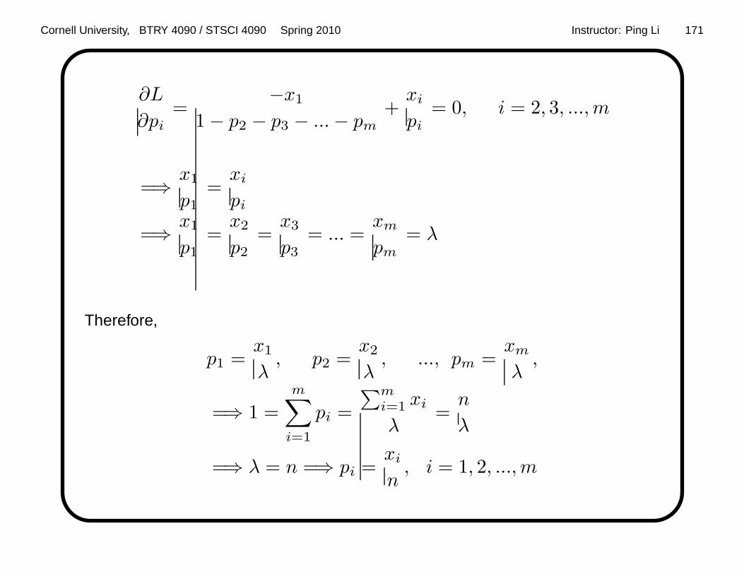
Cornell University, BTRY 4090 / STSCI 4090 Spring 2010 Instructor: Ping Li 171
∂L
∂pi=
−x1
1 − p2 − p3 − ...− pm+xi
pi= 0, i = 2, 3, ...,m
=⇒ x1
p1=xi
pi
=⇒ x1
p1=x2
p2=x3
p3= ... =
xm
pm= λ
Therefore,
p1 =x1
λ, p2 =
x2
λ, ..., pm =
xm
λ,
=⇒ 1 =
m∑
i=1
pi =
∑mi=1 xi
λ=n
λ
=⇒ λ = n =⇒ pi =xi
n, i = 1, 2, ...,m
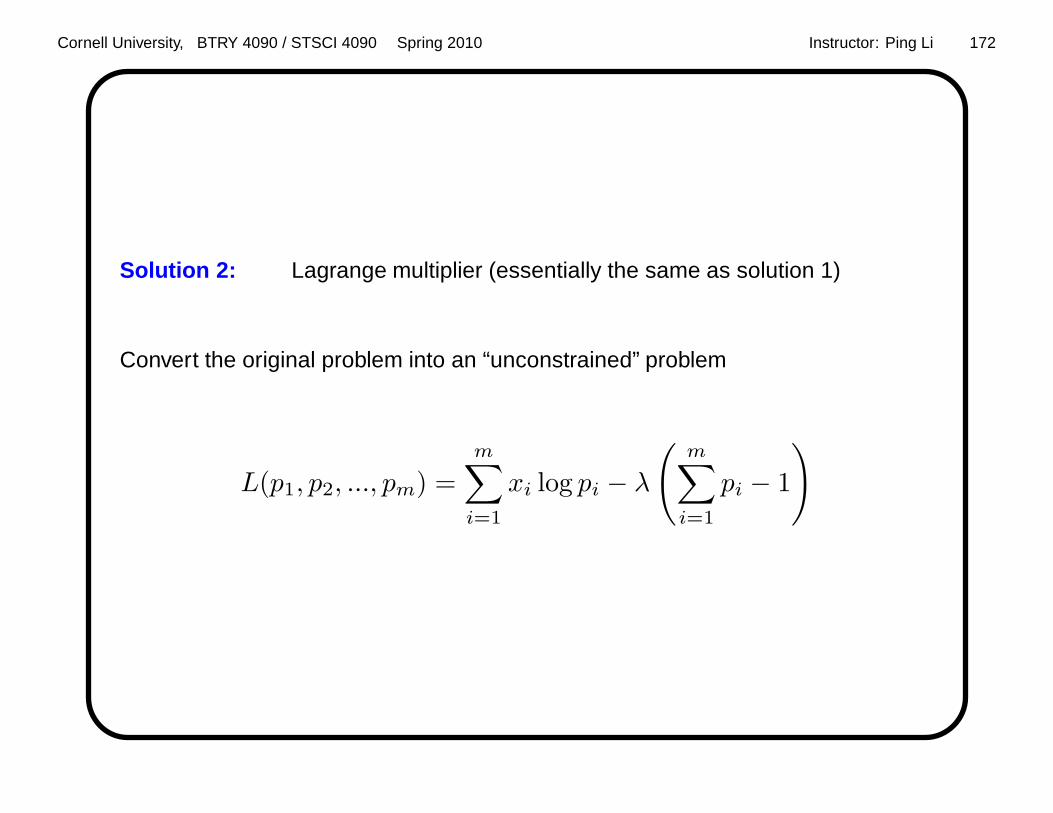
Cornell University, BTRY 4090 / STSCI 4090 Spring 2010 Instructor: Ping Li 172
Solution 2: Lagrange multiplier (essentially the same as solution 1)
Convert the original problem into an “unconstrained” problem
L(p1, p2, ..., pm) =m∑
i=1
xi log pi − λ
(
m∑
i=1
pi − 1
)

Cornell University, BTRY 4090 / STSCI 4090 Spring 2010 Instructor: Ping Li 173
Example A: Hardy-Weinberg Equilibrium
If gene frequencies are in equilibrium, the genotypes AA, Aa, and aa occur in a
population with frequencies
(1 − θ)2, 2θ(1 − θ), θ2,
respectively. Suppose we observe sample counts x1, x2, and x3, with total = n.
Q: Estimate θ using MLE.

Cornell University, BTRY 4090 / STSCI 4090 Spring 2010 Instructor: Ping Li 174
Solution: The log likelihood can be written as
l(θ) =3∑
i=1
xi log pi
=x1 log(1 − θ)2 + x2 log 2θ(1 − θ) + x3 log θ2
∝2x1 log(1 − θ) + x2 log θ + x2 log(1 − θ) + 2x3 log θ
=(2x1 + x2) log(1 − θ) + (x2 + 2x3) log θ
Taking the first derivative
∂l(θ)
∂θ= −2x1 + x2
1 − θ+x2 + 2x3
θ= 0
=⇒ θ =x2 + 2x3
2n
What is V ar(θ)?

Cornell University, BTRY 4090 / STSCI 4090 Spring 2010 Instructor: Ping Li 175
V ar(θ) =1
4n2(V ar(x2) + 4V ar(x3) + 4Cov(x2, x3))
=1
4n2(np2(1 − p2) + 4np3(1 − p3)−4np2p3)
=1
4n
(
p2 + 4p3 − (p2 + 2p3)2)
=θ(1 − θ)
2n
We will soon show the variance of MLE is asymptotically 1I(θ) , where
I(θ) = −E(
∂2l(θ)
∂θ2
)
is the Fisher Information.

Cornell University, BTRY 4090 / STSCI 4090 Spring 2010 Instructor: Ping Li 176
∂2l(θ)
∂θ2= −2x1 + x2
(1 − θ)2− x2 + 2x3
θ2
I(θ) = −E
(
∂2l(θ)
∂θ2
)
=n2(1 − θ)2 + 2θ(1 − θ)
(1 − θ)2+ n
2θ(1 − θ) + 2θ2
θ2
=2n
1 − θ+
2n
θ=
2n
θ(1 − θ)
Therefore, the “asymptotic variance” is V ar(θ) = θ(1−θ)2n ,
which in this case is the exact variance.

Cornell University, BTRY 4090 / STSCI 4090 Spring 2010 Instructor: Ping Li 177
Review Properties of Multinomial Distribution
SupposeX1, X2, ..., Xm, which are the counts of cells 1, 2, ..., m, follow a
multinomial distribution with total count of n and cell probabilities p1, p2, ..., pm.
Marginal and conditional distributions
Xj ∼ Binomial(n, pj)
Xj |Xi ∼ Binomial
(
n−Xi,pj
1 − pi
)
, i 6= j

Cornell University, BTRY 4090 / STSCI 4090 Spring 2010 Instructor: Ping Li 178
Moments
E(Xj) = npj , V ar(Xj) = npj(1 − pj)
E(Xj |Xi) = (n−Xi)pj
1 − pi
E(XiXj) = E(XiE(Xj |Xi)) = E
(
(
nXi −X2i
) pj
1 − pi
)
=pj
1 − pi
(
n2pi − npi(1 − pi) − n2p2i
)
= npipj (n− 1)
Cov(Xi, Xj) = E(XiXj) −E(Xi)E(Xj)
= npipj (n− 1) − n2pipj = −npipj

Cornell University, BTRY 4090 / STSCI 4090 Spring 2010 Instructor: Ping Li 179
Large Sample Theory for MLE
Assume i.i.d. samples of size n, Xi, i = 1 to n, with density f(x|θ).
The MLE of θ, denoted by θ is given by
θ = argmaxθ
n∑
i=1
log f(xi|θ)
Large sample theory says, as n→ ∞, θ is asymptotically unbiased and normal.
θ ∼ N
(
θ,1
nI(θ)
)
, approximately
I(θ) is the Fisher Information of θ: I(θ) = −E[
∂2
∂θ2 log f(X |θ)]
.

Cornell University, BTRY 4090 / STSCI 4090 Spring 2010 Instructor: Ping Li 180
Fisher Information
I(θ) =E
[
∂
∂θlog f(X |θ)
]2
= −E
[
∂2
∂θ2log f(X |θ)
]
How to prove the equivalence of two definitions?

Cornell University, BTRY 4090 / STSCI 4090 Spring 2010 Instructor: Ping Li 181
Proof:
E
[
∂
∂θlog f(X |θ)
]2
=
∫[
∂f
∂θ
]21
f2fdx =
∫[
∂f
∂θ
]21
fdx
−E[
∂2
∂θ2log f(X |θ)
]
= −∫ f ∂2f
∂θ2 −[
∂f∂θ
]2
f2fdx
= −∫
∂2f
∂θ2dx+
∫[
∂f
∂θ
]21
fdx
Therefore, it suffices to show (in fact assume):
∫
∂2f
∂θ2dx =
∂2
∂θ2
[∫
fdx
]
= 0

Cornell University, BTRY 4090 / STSCI 4090 Spring 2010 Instructor: Ping Li 182
Example: Normal Distribution
Given n i.i.d. samples, xi ∼ N(µ, σ2), i = 1 to n.
log fX(x;µ, σ2) = − 1
2σ2(x− µ)2 − 1
2log(2πσ2)
∂2 log fX(x;µ, σ2)
∂µ2= − 1
σ2=⇒ I(µ) =
1
σ2
∂2 log fX(x;µ, σ2)
∂(σ2)2= − (x− µ)2
σ6+
1
2σ4
=⇒ I(σ2) =σ2
σ6− 1
2σ4=
1
2σ4
“Asymptotic” variances of MLE are in fact exact in this case.

Cornell University, BTRY 4090 / STSCI 4090 Spring 2010 Instructor: Ping Li 183
Example: Binomial Distribution
x ∼ Binomial(p, n): Pr (x = k) =(
nk
)
pk(1 − p)n−k
Log likelihood and Fisher Information:
l(p) = k log p+ (n− k) log(1 − p)
l′(p) =k
p− n− k
1 − p=⇒ MLE p =??
l′′(p) = − k
p2− n− k
(1 − p)2
I(p) = −E (l′′(p)) =np
p2+
n− np
(1 − p)2=
n
p(1 − p)
“Asymptotic” variance of MLE is also exact in this case.

Cornell University, BTRY 4090 / STSCI 4090 Spring 2010 Instructor: Ping Li 184
Intuition About the Asymptotic Distributions & Variances o f MLE
The MLE θ is the solution to the MLE equation l′(θ) = 0.
The Taylor expansion around the true θ
l′(θ) ≈ l′(θ) + (θ − θ)l′′(θ)
Let l′(θ) = 0 (because θ is the MLE solution)
(θ − θ) ≈ − l′(θ)
l′′(θ)
What is the mean of l′(θ)? What is the mean of l′′(θ)?

Cornell University, BTRY 4090 / STSCI 4090 Spring 2010 Instructor: Ping Li 185
l′(θ) =n∑
i=1
∂ log f(xi)
∂θ=
n∑
i=1
∂f(xi)∂θ
f(xi)
E (l′(θ)) =n∑
i=1
E
(
∂ log f(xi)
∂θ
)
= nE
(
∂f(x)∂θ
f(x)
)
= 0
because
E
(
∂f(x)∂θ
f(x)
)
=
∫ ∂f(x)∂θ
f(x)f(x)dx =
∫
∂f(x)
∂θdx =
∂
∂θ
∫
f(x)dx = 0

Cornell University, BTRY 4090 / STSCI 4090 Spring 2010 Instructor: Ping Li 186
E(l′(θ)) = 0, and we know −E(l′′(θ)) = nI(θ), the Fisher Information. Thus
(θ − θ) ≈ − l′(θ)
l′′(θ)≈ l′(θ)
nI(θ)
and
E(θ − θ) ≈ E(l′(θ))
nI(θ)= 0
Then, the variance
V ar(θ) ≈ E(l′(θ))2
n2I2(θ)=
nI(θ)
n2I(θ)=
1
nI(θ)

Cornell University, BTRY 4090 / STSCI 4090 Spring 2010 Instructor: Ping Li 187
Sec. 8.7: Efficiency and Cram er-Rao Lower Bound
Definition: Given two unbiased estimates, θ1 and θ2, the efficiency of θ1
relative to θ2 is
eff(
θ1, θ2
)
=V ar(θ2)
V ar(θ1)
For example, if the variance of θ2 is 0.8 times the variance of θ1. Then θ1 is 80%
efficient relative to θ2.
Asymptotic relative efficiency Given two asymptotically unbiased
estimates, θ1 and θ2, the asymptotic relative efficiency of θ1 relative to θ2 is
computed using their asymptotic variances (as sample size goes to infinity).
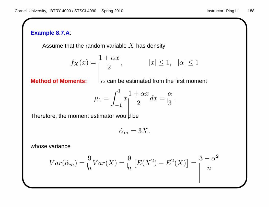
Cornell University, BTRY 4090 / STSCI 4090 Spring 2010 Instructor: Ping Li 188
Example 8.7.A :
Assume that the random variable X has density
fX(x) =1 + αx
2, |x| ≤ 1, |α| ≤ 1
Method of Moments: α can be estimated from the first moment
µ1 =
∫ 1
−1
x1 + αx
2dx =
α
3.
Therefore, the moment estimator would be
αm = 3X.
whose variance
V ar(αm) =9
nV ar(X) =
9
n
[
E(X2) −E2(X)]
=3 − α2
n

Cornell University, BTRY 4090 / STSCI 4090 Spring 2010 Instructor: Ping Li 189
Maximum Likelihood Estimate: The first two derivatives
∂
∂αlog fX(x;α) =
x
1 + αx
∂2
∂α2log fX(x;α) =
−x2
(1 + αx)2
Therefore, the MLE is the solution to
n∑
i=1
Xi
1 + αmleXi= 0.
Can not compute the exact variance. We resort to approximate (asymptotic)
variance
V ar (αmle) ≈1
nI(α)

Cornell University, BTRY 4090 / STSCI 4090 Spring 2010 Instructor: Ping Li 190
Use the second derivatives to compute I(α)
I(α) = − E
[
∂2
∂α2log fX(x|α)
]
=
∫ 1
−1
x2
(1 + αx)21 + αx
2dx
=
∫ 1
−1
x2
2(1 + αx)dx
=log 1+α
1−α − 2α
2α3, α 6= 0
When α = 0, I(α) =∫ 1
−1x2
2 dx = 13 ,
which can also be obtained by taking limit of I(α).

Cornell University, BTRY 4090 / STSCI 4090 Spring 2010 Instructor: Ping Li 191
The asymptotic relative efficiency of αm to αmle is
V ar(αmle)
V ar(αm)=
2α3
3−α2
log 1+α1−α − 2α
−1 −0.5 0 0.5 10
0.1
0.2
0.3
0.4
0.5
0.6
0.7
0.8
0.9
1
α
Effi
cien
cy
Why the efficiency is no larger than 1?

Cornell University, BTRY 4090 / STSCI 4090 Spring 2010 Instructor: Ping Li 192
Cramer-Rao Inequality
Theorem 8.7.A: Let X1, X2, ..., Xn be i.i.d. with density function f(x; θ).
Let T be an unbiased estimate of θ. Then under smoothness assumption on
f(x; θ),
V ar(T ) ≥ 1
nI(θ)
Thus, under reasonable assumptions, MLE is optimal or (asymptotically) optimal.

Cornell University, BTRY 4090 / STSCI 4090 Spring 2010 Instructor: Ping Li 193
Sec. 8.8: Sufficiency
Definition: LetX1, X2, ..., Xn be i.i.d. samples with density f(x; θ). A
statistic T = T (X1, X2, ..., Xn) is said to be sufficient for θ if the conditional
distribution of X1, X2, ..., Xn, given T = t, does not depend on θ for any t.
In other words, given T , we can gain no more knowledge about θ.

Cornell University, BTRY 4090 / STSCI 4090 Spring 2010 Instructor: Ping Li 194
Example 8.8.A: LetX1, X2, ..., Xn be a sequence of independent
Bernoulli random variables with P (Xi = 1) = θ. Let T =∑n
i=1Xi.
P (X1 = x1, ..., Xn = xn|T = t) =P (X1 = x1, ..., Xn = xn, T = t)
P (T = t)
=θt(1 − θ)n−t
(
nt
)
θt(1 − θ)n−t
=1(
nt
) ,
which is independent of θ. Therefore, T =∑n
i=1Xi is a sufficient statistic.

Cornell University, BTRY 4090 / STSCI 4090 Spring 2010 Instructor: Ping Li 195
Theorem 8.8.1.A: Factorization Theorem
A necessary and sufficient condition for T (X1, ..., Xn) to be sufficient for a
parameter θ is that the joint probability density (mass) function factors
f(x1, x2, .., xn; θ) = g [T (x1, x2, ..., xn), θ]h(x1, x2, ..., xn)

Cornell University, BTRY 4090 / STSCI 4090 Spring 2010 Instructor: Ping Li 196
Example 8.8.1.A: X1, X2, ..., Xn are i.i.d. Bernoulli random variables with
success probability θ.
f(x1, x2, ..., xn; θ) =θ∏
i=1
θxi(1 − θ)1−xi
=θ∑n
i=1 xi(1 − θ)n−∑ni=1 xi
=
(
θ
1 − θ
)
∑ni=1 xi
(1 − θ)n
=g (T, θ) × h
h(x1, x2, ..., xn) = 1.
T (x1, x2, ..., xn) =∑n
i=1 xi is the sufficient statistic.
g(T, θ) =(
θ1−θ
)T
(1 − θ)n

Cornell University, BTRY 4090 / STSCI 4090 Spring 2010 Instructor: Ping Li 197
Example 8.8.1.B: X1, X2, ..., Xn are i.i.d. normalN(µ, σ2), both µ and
σ2 are unknown.
f(x1, x2, ..., xn;µ, σ2) =n∏
i=1
1√2πσ
e−(xi−µ)2
2σ2
=1
(2π)n/2σne−
∑ni=1
(xi−µ)2
2σ2
=1
(2π)n/2σne
−1
2σ2 [∑n
i=1 x2i−2µ
∑ni=1 xi+nµ2]
Therefore,∑n
i=1 x2i and
∑ni=1 xi are sufficient statistics.
Equivalently, we say T = (X, S2) is the sufficient statistic for normal with
unknown mean and variance.

Cornell University, BTRY 4090 / STSCI 4090 Spring 2010 Instructor: Ping Li 198
Proof of the Factorization Theorem (Discrete Case)
Theorem: A necessary and sufficient condition for T (X1, ..., Xn) to be
sufficient for a parameter θ is that the joint probability mass function factors
P (X1 = x1, .., Xn = xn; θ) = g [T (x1, ..., xn), θ]h(x1, ..., xn)
Proof of sufficient condition: Assume
P (X1 = x1, .., Xn = xn; θ) = g [T (x1, ..., xn), θ]h(x1, ..., xn)
Then the conditional distribution
P (X1 = x1, ..., Xn = xn|T = t) =P (X1 = x1, ..., Xn = xn, T = t)
P (T = t)

Cornell University, BTRY 4090 / STSCI 4090 Spring 2010 Instructor: Ping Li 199
But we assume P (X1, .., Xn) factors, i.e.,
P (T = t) =∑
T (x1,...,xn)=t
P (X1 = x1, ..., Xn = xn)
=g(t, θ)∑
T (x1,...,xn)=t
h(x1, ..., xn)
Note that t is constant. Thus, the conditional distribution
P (X1 = x1, ..., Xn = xn|T = t) =P (X1 = x1, ..., Xn = xn, T = t)
P (T = t)
=g(t, θ)h(x1, ..., xn)
∑
T (x1,...,xn)=t g(t, θ)h(x1, ..., xn)
=h(x1, ..., xn)
∑
T (x1,...,xn)=t h(x1, ..., xn),
which does not depend on θ.
Therefore, T (X1, ..., Xn) is a sufficient statistic.

Cornell University, BTRY 4090 / STSCI 4090 Spring 2010 Instructor: Ping Li 200
Proof of necessary condition: Assume T (X1, ..., Xn) is sufficient. That
is, the conditional distribution (X1, ..., Xn)|T does not depend on θ. Then
P (X1 = x1, ..., Xn = xn) =P (X1 = x1, ..., Xn = xn|T = t)P (T = t)
=P (T = t)P (X1 = x1, ..., Xn = xn|T = t)
=g(t, θ)h(x1, ..., xn),
where
h(x1, ..., xn) = P (X1 = x1, ..., Xn = xn|T = t)
g(t, θ) = P (T = t)
Therefore, the probability mass function factors.

Cornell University, BTRY 4090 / STSCI 4090 Spring 2010 Instructor: Ping Li 201
Exponential Family
Definition: Members of one parameter (θ) exponential family have density
function (or frequency functions) of the form
f(x; θ) =
exp [c(θ)T (x) + d(θ) + S(x)] if x ∈ A
0 otherwise
Where the setA does not depend on θ.
Many common distributions: normal, binomial, Poisson, gamma, are members of
this family.

Cornell University, BTRY 4090 / STSCI 4090 Spring 2010 Instructor: Ping Li 202
Example 8.8.C : The frequency function of the Bernoulli distribution is
P (X = x) =θx(1 − θ)1−x, x ∈ 0, 1
=exp
[
x logθ
1 − θ+ log(1 − θ)
]
Therefore, this is a member of the exponential family, with
c(θ) = logθ
1 − θ
T (x) = x
d(θ) = log 1 − θ
S(x) = 0.
—————-
f(x; θ) = exp [c(θ)T (x) + d(θ) + S(x)].

Cornell University, BTRY 4090 / STSCI 4090 Spring 2010 Instructor: Ping Li 203
Sufficient statistics of exponential family
Suppose thatX1, X2, ..., Xn is an i.i.d. sample from a member of the
exponential family. Then the joint probability is
n∏
i=1
f(xi|θ) =n∏
i=1
exp [c(θ)T (xi) + d(θ) + S(xi)]
= exp
[
c(θ)n∑
i=1
T (xi) + nd(θ)
]
exp
[
n∑
i=1
S(xi)
]
By the factorization theorem, we know∑n
i=1 T (xi) is a sufficient statistic.
In the Bernoulli example,∑n
i=1 T (xi) =∑n
i=1 xi.

Cornell University, BTRY 4090 / STSCI 4090 Spring 2010 Instructor: Ping Li 204
The MLE of exponential family
If T (x) is a sufficient statistic for θ, then the MLE is a function of T .
Recall: if X ∼ N(µ, σ2), then the MLE
µ =1
n
n∑
i=1
xi
σ2 =1
n
n∑
i=1
(xi − µ)2
We know that (∑n
i=1 xi,∑n
i=1 x2i ) is sufficient statistic.
Note that normal is a member of the two-parameter exponential family.

Cornell University, BTRY 4090 / STSCI 4090 Spring 2010 Instructor: Ping Li 205
k-parameter Exponential Family
Definition: Members of k-parameter (θ) exponential family have density
function (or frequency functions) of the form
f(x; θ) = exp
k∑
j=1
cj(θ)Tj(x) + d(θ) + S(x)

Cornell University, BTRY 4090 / STSCI 4090 Spring 2010 Instructor: Ping Li 206
Normal Distribution and Exponential Family
SupposeX ∼ N(µ, σ2). Then
f(x;µ, σ2) =1√2π
exp
[
−1
2log σ2 − 1
2σ2x2 +
µ
σ2x− µ2
2σ2
]
Does it really belong to a (2-dim) exponential family?
Well, suppose σ2 is known, then it is clear that it does belong to a one-dim
exponential family.
f(x; θ) = exp [c(θ)T (x) + d(θ) + S(x)]
θ = µ, T (x) = x, c(θ) =µ
σ2
d(θ) = − µ2
2σ2, S(x) = − x2
2σ2− 1
2log σ2 − 1
2log 2π

Cornell University, BTRY 4090 / STSCI 4090 Spring 2010 Instructor: Ping Li 207
When σ2 is unknown, then we need to re-parameterize the distribution by letting
θ =( µ
σ2, σ2)
= (θ1, θ2)
Then it belongs to a 2-dim exponential family
f(x; θ) = exp [c1(θ)T1(x) + c2(θ)T2(x) + d(θ) + S(x)]
c1(θ) =µ
σ2= θ1, T1(x) = x
c2(θ) = − 1
2σ2= − 1
2θ2, T2(x) = x2
d(θ) = −1
2log σ2 − µ2
2σ2= −1
2log θ2 −
θ21
2θ2
S(x) = −1
2log 2π

Cornell University, BTRY 4090 / STSCI 4090 Spring 2010 Instructor: Ping Li 208
Another Nice Property of Exponential Family
Suppose
f(x; θ) = exp
k∑
j=1
cj(θ)Tj(x) + d(θ) + S(x)
Then
E (Ti(X)) = − ∂d(θ)
∂ci(θ)
Exercise: What about variances and covariances?

Cornell University, BTRY 4090 / STSCI 4090 Spring 2010 Instructor: Ping Li 209
Proof: Take derivatives on both sides of∫
fdx = 1, i.e.,∂∫
fdx∂ci(θ) = 0.
∂∫
fdx
∂ci(θ)=
∫
∂f
∂ci(θ)dx
=
∫
∂
∂ci(θ)exp
k∑
j=1
cj(θ)Tj(x) + d(θ) + S(x)
dx
=
∫
exp
k∑
j=1
cj(θ)Tj(x) + d(θ) + S(x)
[
Ti(x) +∂d(θ)
∂ci(θ)
]
dx
=
∫
f
[
Ti(x) +∂d(θ)
∂ci(θ)
]
dx
Therefore
E (Ti(X)) =
∫
fTi(x)dx = −∫
f∂d(θ)
∂ci(θ)dx = − ∂d(θ)
∂ci(θ)

Cornell University, BTRY 4090 / STSCI 4090 Spring 2010 Instructor: Ping Li 210
For example,X ∼ N(µ, σ2) belongs to a 2-dim exponential family
θ = (θ1, θ2) =( µ
σ2, σ2)
T1(x) = x, T2(x) = x2
Apply the previous result,
E(T1(x)) = E(x) = −∂d(θ)c1(θ)
= − (−θ1θ2) =µ
σ2σ2 = µ
as expected.
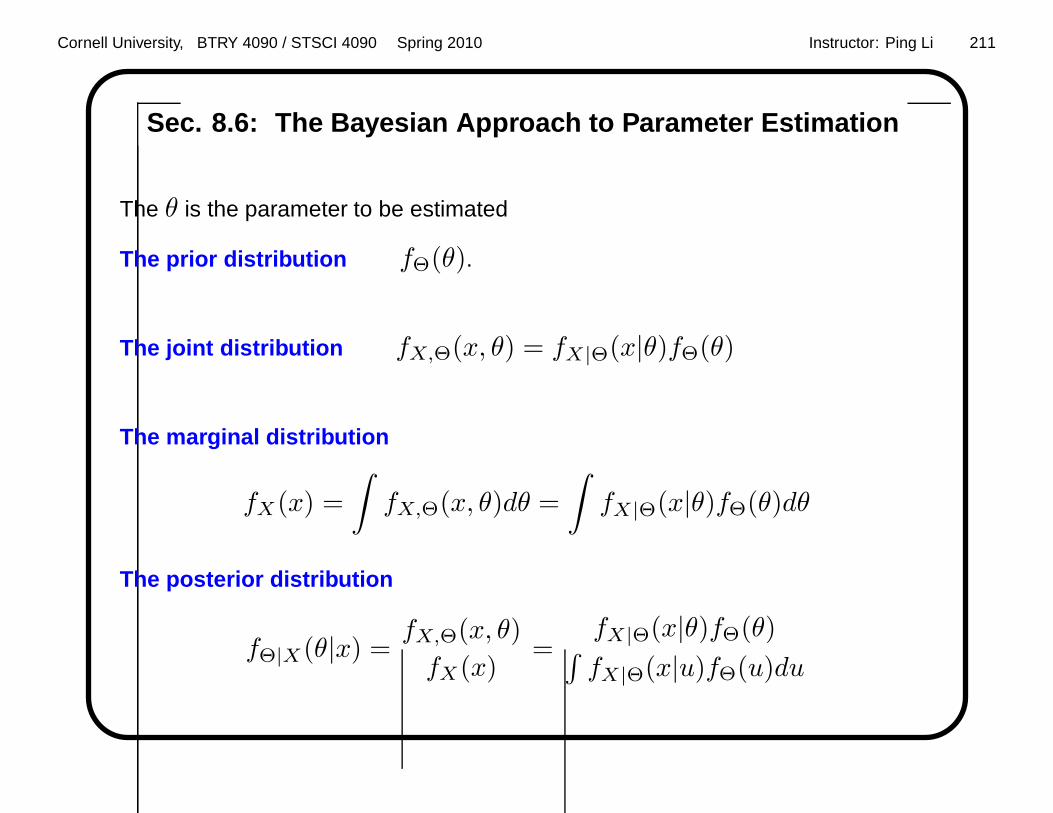
Cornell University, BTRY 4090 / STSCI 4090 Spring 2010 Instructor: Ping Li 211
Sec. 8.6: The Bayesian Approach to Parameter Estimation
The θ is the parameter to be estimated
The prior distribution fΘ(θ).
The joint distribution fX,Θ(x, θ) = fX|Θ(x|θ)fΘ(θ)
The marginal distribution
fX(x) =
∫
fX,Θ(x, θ)dθ =
∫
fX|Θ(x|θ)fΘ(θ)dθ
The posterior distribution
fΘ|X(θ|x) =fX,Θ(x, θ)
fX(x)=
fX|Θ(x|θ)fΘ(θ)∫
fX|Θ(x|u)fΘ(u)du

Cornell University, BTRY 4090 / STSCI 4090 Spring 2010 Instructor: Ping Li 212
Three main issues in Bayesian estimation
• Specify a prior (without looking at the data first).
• Calculate the posterior distribution, maybe computationally intensive.
• Choose appropriate estimators from the posterior distribution:
mean, median, mode, ...

Cornell University, BTRY 4090 / STSCI 4090 Spring 2010 Instructor: Ping Li 213
The Add-one Smoothing
Consider n+m trials having a common probability of success. Suppose,
however, that this success probability is not fixed in advance but is chosen from
U(0, 1).
Q: What is the conditional distribution of this success probability given that the
n+m trials result in n successes?
Solution:
Let X = trial success probability. X ∼ U(0, 1).
Let N = total number of successes. N |X = x ∼ Binomial(n+m,x).

Cornell University, BTRY 4090 / STSCI 4090 Spring 2010 Instructor: Ping Li 214
Solution:
Let X = trial success probability. X ∼ U(0, 1).
Let N = total number of successes. N |X = x ∼ Binomial(n+m,x).
fX|N (x|n) =PN = n|X = xfX(x)
PN = n
=
(
n+mn
)
xn(1 − x)m
PN = n∝ xn(1 − x)m
Therefore,X |N ∼ Beta(n+ 1,m+ 1).
Here X ∼ U(0, 1) is the prior distribution.

Cornell University, BTRY 4090 / STSCI 4090 Spring 2010 Instructor: Ping Li 215
If X |N ∼ Beta(n+ 1,m+ 1), then
E(X |N) =n+ 1
(n+ 1) + (m+ 1)
Suppose we do not have a prior knowledge of the success probability X .
We observe n successes out of n+m trials.
The most intuitive estimate (in fact MLE) of X should be
X =n
n+m
Assuming a uniform prior on X leads to the add-one smoothing .

Cornell University, BTRY 4090 / STSCI 4090 Spring 2010 Instructor: Ping Li 216
0 0.2 0.4 0.6 0.8 10
1
2
3
4
5
6
7
8
9
10Posterior distribution, assuming p ~ U(0,1)
p
PM
F
m = 8, n = 0m = 8, n = 2m = 80, n = 20
Posterior distribution X |N ∼ Beta(n+ 1,m+ 1).
Posterior mean: E(X) = n+1m+1 ,
Posterior mode (peak of density): nm .

Cornell University, BTRY 4090 / STSCI 4090 Spring 2010 Instructor: Ping Li 217
Estimating Binomial Parameter Under Beta Prior
X ∼ Bin(n, p). p ∼ Beta(a, b).
Joint probability
fX,P (x, p) =
[(
n
x
)
px(1 − p)n−x
] [
Γ(a+ b)
Γ(a)Γ(b)pa−1(1 − p)b−1
]
=Γ(a+ b)
Γ(a)Γ(b)
(
n
x
)
[
px+a−1(1 − p)n−x+b−1]
which is also a beta distribution Beta(x+ a, n− x+ b).
Marginal distribution
fX(x) =
∫ 1
0
fX,P (x, p)dp = g(n, x), (very nice, why?)
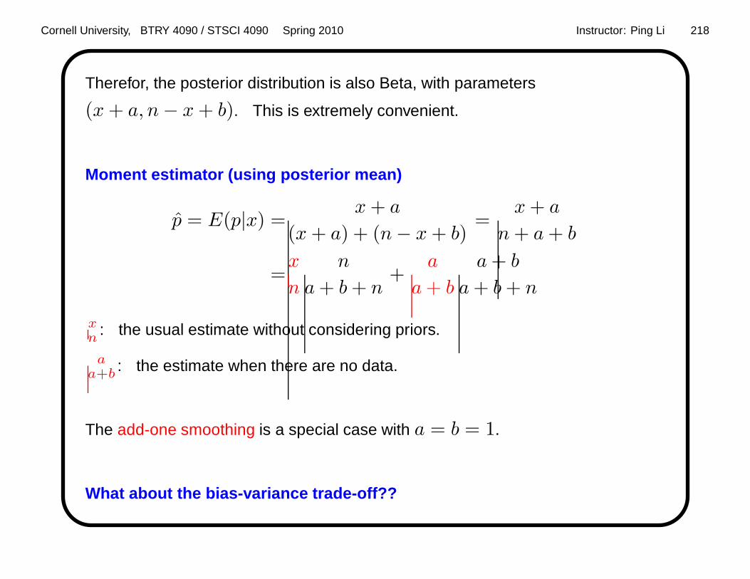
Cornell University, BTRY 4090 / STSCI 4090 Spring 2010 Instructor: Ping Li 218
Therefor, the posterior distribution is also Beta, with parameters
(x+ a, n− x+ b). This is extremely convenient.
Moment estimator (using posterior mean)
p = E(p|x) =x+ a
(x+ a) + (n− x+ b)=
x+ a
n+ a+ b
=x
n
n
a+ b+ n+
a
a+ b
a+ b
a+ b+ n
xn : the usual estimate without considering priors.
aa+b : the estimate when there are no data.
The add-one smoothing is a special case with a = b = 1.
What about the bias-variance trade-off??

Cornell University, BTRY 4090 / STSCI 4090 Spring 2010 Instructor: Ping Li 219
The Bias-Variance Trade-off
Bayesian estimator (using posterior mean)
p =x+ a
n+ a+ b
MLE
pMLE =x
n
Assume p is fixed (conditional on p). Study the MSE ratio
MSE ratio =MSE(p)
MSE(pMLE)
We hope MSE ratio ≤ 1, especially when sample size n is reasonable.

Cornell University, BTRY 4090 / STSCI 4090 Spring 2010 Instructor: Ping Li 220
Asymptotic MSE ratio : when n is not too small
Asymptotic MSE ratio = 1 +A
n+O
(
1
n2
)
.
We hopeA ≤ 0
Exercise : Find A, which is a function of p, a, b.

Cornell University, BTRY 4090 / STSCI 4090 Spring 2010 Instructor: Ping Li 221
0 20 40 60 80 1000
0.1
0.2
0.3
0.4
0.5
0.6
0.7
0.8
0.9
1
n
p = 0.5 , a = 1 , b = 1
MS
E r
atio
s
Exact MSE ratiosAsymptotic MSE ratios

Cornell University, BTRY 4090 / STSCI 4090 Spring 2010 Instructor: Ping Li 222
0 20 40 60 80 1000.5
1
1.5
2
n
MS
E r
atio
s
p = 0.9 , a = 1 , b = 1
Exact MSE ratiosAsymptotic MSE ratios

Cornell University, BTRY 4090 / STSCI 4090 Spring 2010 Instructor: Ping Li 223
Conjugate Priors
The prior distribution fΘ(θ), belongs to family G.
The conditional distribution fX|Θ(x|θ), belongs to family H .
The posterior distribution
fΘ|X(θ|x) =fX,Θ(x, θ)
fX(x)=
fX|Θ(x|θ)fΘ(θ)∫
fX|Θ(x|u)fΘ(u)du
If the posterior distribution also belongs to G, then G is conjugate to H .
Conjugate priors were introduced mainly for the computational convenience.

Cornell University, BTRY 4090 / STSCI 4090 Spring 2010 Instructor: Ping Li 224
Examples of Conjugate priors:
Beta is conjugate to Binomial.
Gamma is conjugate to Poisson.
Dirichlet is conjugate to multinomial.
Gamma is conjugate to exponential.
Normal is conjugate to normal (with known variance).

Cornell University, BTRY 4090 / STSCI 4090 Spring 2010 Instructor: Ping Li 225
Chapter 9: Testing Hypothesis
Suppose you have a coin which is possibly biased. You want to test whether the
coin is indeed biased (i.e., p 6= 0.5), by tossing the coin n = 10 times.
Suppose you observe k = 8 heads (out of n = 10 tosses). It is reasonable to
guess that this coin is indeed biased. But how to make a precise statement?
Are n = 10 tosses enough? How about n = 100? n = 1000? What is the
principled approach?

Cornell University, BTRY 4090 / STSCI 4090 Spring 2010 Instructor: Ping Li 226
Terminologies
Null hypothesis H0 : p = 0.5
Alternative hypothesis HA : p 6= 0.5
Type I error RejectingH0 when it is true
Significance level P (Type I error) = P (RejectH0|H0) = α
Type II error AcceptingH0 when it is false
P (Type II error) = P (AcceptH0|HA) = β
Power 1 − β
Goal: Low α and high 1 − β.

Cornell University, BTRY 4090 / STSCI 4090 Spring 2010 Instructor: Ping Li 227
Example 9.2.A LetX1, X2, ..., Xn be an i.i.d. sample from a normal with
known variance σ2 and unknown mean µ. Consider two simple hypotheses :
H0 : µ = µ0
HA : µ = µ1 (µ1 > µ0)
Under H0, the null distribution likelihood is
f0 ∝n∏
i=1
exp
[
− 1
2σ2(Xi − µ0)
2
]
= exp
[
− 1
2σ2
n∑
i=1
(Xi − µ0)2
]
Under HA, the likelihood is
f1 ∝ exp
[
− 1
2σ2
n∑
i=1
(Xi − µ1)2
]
Which hypothesis is more likely?

Cornell University, BTRY 4090 / STSCI 4090 Spring 2010 Instructor: Ping Li 228
Likelihood Ratio : Small ratios =⇒ rejection. Sounds reasonable, but why?
f0f1
=exp
[
− 12σ2
∑ni=1(Xi − µ0)
2]
exp[
− 12σ2
∑ni=1(Xi − µ1)2
]
= exp
[
− 1
2σ2
n∑
i=1
[
(Xi − µ0)2 − (Xi − µ1)
2]
]
= exp[ n
2σ2
[
2X(µ0 − µ1) + µ21 − µ2
0
]
]
Because µ0 − µ1 < 0 (by assumption), the likelihood is small if X is large.
Suppose the significance level α = 0.05. With how large X can we reject H0?
Neyman-Pearson Lemma provides the answers.

Cornell University, BTRY 4090 / STSCI 4090 Spring 2010 Instructor: Ping Li 229
Neyman-Pearson Lemma
Suppose thatH0 and HA are simple hypotheses and that the test that rejects
H0 whenever the likelihood ratio is less than c has significance level α. Then any
other test for which the significance level is ≤ α has power less than or equal to
that of the likelihood ratio test.
In other words, among all possible tests achieving significance level ≤ α, the test
based on likelihood ratio maximizes the power.

Cornell University, BTRY 4090 / STSCI 4090 Spring 2010 Instructor: Ping Li 230
Proof: Let H0 : f(x) = f0(x), HA : f(x) = fA(x)
Denote two tests
d(x) =
0, if H0 is accepted
1, if H0 is rejectedd∗(x) =
0, if H0 is accepted
1, if H0 is rejected
The test d(x), based on the likelihood ratio, has a significance level α, i.e.,
d(x) = 1, whenever f0(x) < cfA(x), (c > 0)
α = P (d(x) = 1|H0) = E(d(x)|H0) =
∫
d(x)f0(x)dx
Assume the test d∗(x) has smaller significance level, i.e.,
P (d∗(x) = 1|H0) ≤ P (d(x) = 1|H0) = α
=⇒∫
[d(x) − d∗(x)] f0(x)dx ≥ 0

Cornell University, BTRY 4090 / STSCI 4090 Spring 2010 Instructor: Ping Li 231
To show: P (d∗(x) = 1|HA)≤P (d(x) = 1|HA)
Equivalently, we need to show∫
[d(x) − d∗(x)] fA(x)dx≥0
We make use of a key inequality
d∗(x) [cfA(x) − f0(x)] ≤ d(x) [cfA(x) − f0(x)]
which is true because d(x) = 1 whenever cfA(x) − f0(x) > 0, and
d(x), d∗(x) only take values in 0, 1.
More specifically, let M(x) = cfA(x) − f0(x).
If M(x) > 0, then the right-hand-side of the inequality becomesM(x), but the
left-hand-side becomesM(x) (if d∗(x) = 1) or 0 (if d∗(x) = 0). Thus the
inequality holds, becauseM(x) > 0.

Cornell University, BTRY 4090 / STSCI 4090 Spring 2010 Instructor: Ping Li 232
If M(x) < 0, then the right-hand-side of the inequality becomes 0, but the
left-hand-side becomesM(x) (if d∗(x) = 1) or 0 (if d∗(x) = 0). Thus the
inequality also holds, becauseM(x) < 0.
Integrating both sides of the inequality yields∫
d∗(x) [cfA(x) − f0(x)] dx ≤∫
d(x) [cfA(x) − f0(x)] dx
=⇒c
∫
[d(x) − d∗(x)] fAdx ≥∫
[d(x) − d∗(x)] f0dx ≥ 0

Cornell University, BTRY 4090 / STSCI 4090 Spring 2010 Instructor: Ping Li 233
Continue Example 9.2.A : f0
f1≤ c=⇒ RejectH0.
f0f1
= exp[ n
2σ2
[
2X(µ0 − µ1) + µ21 − µ2
0
]
]
≤ c
α = P (rejectH0|H0) = P (f0 ≤ cf1|H0)
Equivalently,
RejectH0 if X ≥ x0, and
P (X ≥ x0|H0) = α.
Under H0: X ∼ N(
µ0, σ2/n)

Cornell University, BTRY 4090 / STSCI 4090 Spring 2010 Instructor: Ping Li 234
α =P (X ≥ x0|H0)
=P
(
X − µ0
σ/√n
>x0 − µ0
σ/√n
)
=1 − Φ
(
x0 − µ0
σ/√n
)
=⇒ x0 = µ0 + zασ√n
zα is the upper α point of the standard normal:
P (Z ≥ zα) = α, where Z ∼ N(0, 1). z0.05 = 1.645, z0.025 = 1.960
Therefore, the test rejects H0 if X ≥ µ0 + zασ√n
.
—————
Q: What is β? What is the power? Can we reduce both α and β when n is fixed?

Cornell University, BTRY 4090 / STSCI 4090 Spring 2010 Instructor: Ping Li 235
Uniformly Most Powerful Test
Neyman-Pearson Lemma requires that both hypotheses be simple. However,
most real-situations require composite hypothesis.
If the alternative H1 is composite, a test that is most powerful for every simple
alternative in H1 is uniformly most powerful (UMP).

Cornell University, BTRY 4090 / STSCI 4090 Spring 2010 Instructor: Ping Li 236
Continuing Example 9.2.A: Consider testing
H0 : µ = µ0
H1 : µ > µ0
For every µ1 > µ0, the likelihood ratio test rejects H0 if X ≥ x0, where
x0 = µ0 + zασ√n
does not depend on µ1.
Therefore, this test is most powerful for every µ1 > µ0 and hence it is UMP.

Cornell University, BTRY 4090 / STSCI 4090 Spring 2010 Instructor: Ping Li 237
Similarly, the test is UMP for testing (one-sided alternative)
H0 : µ < µ0
H1 : µ > µ0
However, the test is not UMP for testing (two-sided alternative)
H0 : µ = µ0
H1 : µ 6= µ0
Unfortunately, in typical composite situations, there is no UMP test.

Cornell University, BTRY 4090 / STSCI 4090 Spring 2010 Instructor: Ping Li 238
P-Value
Definition: The p-value is the smallest significance level at which the null
hypothesis would be rejected.
The smaller the p-value, the stronger the evidence against the null hypothesis.
In a sense, calculating the p-value is more sensible than specifying (often
arbitrarily) the level of significance α.

Cornell University, BTRY 4090 / STSCI 4090 Spring 2010 Instructor: Ping Li 239
Confidence Intervals
Example 9.3 A: LetX1, ... Xn be an i.i.d. sample from a normal distribution
having unknown mean µ and known variance σ2. Consider testing
H0 : µ = µ0
HA : µ 6= µ0
Consider a test that rejects H0: for |X − µ0| ≥ x0 such that
P (|X − µ0| > x0|H0) = α
Solve for x0: x0 = σ√nzα/2.

Cornell University, BTRY 4090 / STSCI 4090 Spring 2010 Instructor: Ping Li 240
The test acceptsH0 if
X − σ√nzα/2 ≤ µ0 ≤ X +
σ√nzα/2
We say a 100(1 − α)% confidence interval for µ0 is
µ0 ∈[
X − σ√nzα/2, X +
σ√nzα/2
]
Duality: µ0 lies in the confidence interval for µ if and only if the hypothesis
test accepts. This result holds more generally.

Cornell University, BTRY 4090 / STSCI 4090 Spring 2010 Instructor: Ping Li 241
Duality of Confidence Intervals and Hypothesis Tests
Let θ be a parameter of a family of probability distributions. θ ∈ Θ. Denote the
random variables constituting the data by X.
Theorem 9.3.A: Suppose that for every value θ0 ∈ Θ there is a test at level
α of the hypothesis: H0 : θ = θ0. Denote that acceptance region of the test by
A(θ0). Then the set
C(X) = θ : X ∈ A(θ)
is a 100(1 − α)% confidence region for θ.

Cornell University, BTRY 4090 / STSCI 4090 Spring 2010 Instructor: Ping Li 242
Proof: Need to show
P [θ0 ∈ C(X)|θ = θ0] = 1 − α
By the definition of C(X), we know
P [θ0 ∈ C(X)|θ = θ0] = P [X ∈ A(θ0)|θ = θ0]
By the definition of level of significance, we know
P [X ∈ A(θ0)|θ = θ0] = 1 − α.
This completes the proof.

Cornell University, BTRY 4090 / STSCI 4090 Spring 2010 Instructor: Ping Li 243
Theorem 9.3.B: Suppose that C(X) is 100(1 − α)% confidence region for
θ; that is, for every θ0,
P [θ0 ∈ C(X)|θ = θ0] = 1 − α
Then an acceptance region for a test at level α of H0 : θ = θ0 is
A(θ0) = X|θ0 ∈ C(X)
Proof:
P [X ∈ A(θ0)|θ = θ0] = P [θ0 ∈ C(X)|θ = θ0] = 1 − α

Cornell University, BTRY 4090 / STSCI 4090 Spring 2010 Instructor: Ping Li 244
Generalized Likelihood Ratio Test
Likelihood ratio test :
A simple hypothesis versus a simple hypothesis. Optimal. Very limited use.
Generalized likelihood ratio test:
Composite hypotheses. Sub-optimal and widely-used.
Play the same role as MLE in parameter estimation.

Cornell University, BTRY 4090 / STSCI 4090 Spring 2010 Instructor: Ping Li 245
Assume a sampleX1, ... ,Xn from a distribution with unknown parameter θ.
H0 : θ ∈ ω0
HA : θ ∈ ω1
Let Ω = ω0 ∪ ω1. The test statistic
Λ =
maxθ∈ω0
lik(θ)
maxθ∈Ω
lik(θ)
RejectH0 if Λ ≤ λ0, such that
P (Λ ≤ λ0|H0) = α

Cornell University, BTRY 4090 / STSCI 4090 Spring 2010 Instructor: Ping Li 246
Example 9.4.A: Testing a Normal Mean Let X1, ..., Xn be i.i.d. and
normally distributed with mean µ and known variance σ2. Test
H0 : µ = µ0
HA : µ 6= µ0
In other words, ω0 = µ0, Ω = −∞ < µ <∞.
maxθ∈ω0
lik(µ) =1
(√2πσ
)n e− 1
2σ2
∑ni=1(Xi−µ0)
2
maxθ∈Ω
lik(µ) =1
(√2πσ
)n e− 1
2σ2
∑ni=1(Xi−X)2

Cornell University, BTRY 4090 / STSCI 4090 Spring 2010 Instructor: Ping Li 247
Λ =
maxθ∈ω0
lik(θ)
maxθ∈Ω
lik(θ)= exp
− 1
2σ2
[
n∑
i=1
(Xi − µ0)2 −
n∑
i=1
(Xi − X)2
]
=exp
− 1
2σ2
[
n∑
i=1
(X − µ0)(2Xi − µ0 − X)
]
=exp
− 1
2σ2
[
n(X − µ0)2]
−2 log Λ =(X − µ0)
2
σ2/n
Because underH0, ∼ N(µ0, σ2/n), we know, underH0,
−2 log Λ|H0 ∼ χ21
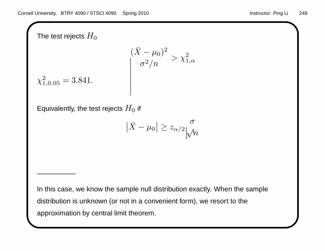
Cornell University, BTRY 4090 / STSCI 4090 Spring 2010 Instructor: Ping Li 248
The test rejects H0
(X − µ0)2
σ2/n> χ2
1,α
χ21,0.05 = 3.841.
Equivalently, the test rejects H0 if
∣
∣X − µ0
∣
∣ ≥ zα/2σ√n
—————–
In this case, we know the sample null distribution exactly. When the sample
distribution is unknown (or not in a convenient form), we resort to the
approximation by central limit theorem.

Cornell University, BTRY 4090 / STSCI 4090 Spring 2010 Instructor: Ping Li 249
Theorem 9.4.A: Under some smoothness conditions on the probability
density of mass functions, the null distribution of −2 log Λ tends to a chi-square
distribution with degrees of freedom equal to dimΩ− dimω0, as the sample size
tends to infinity.
dimΩ = number of free parameters under Ω
dimω0 = number of free parameters under ω0.
In Example 9.4.A, the null hypothesis specifies µ and σ2 and hence there are no
free parameters underH0, i.e., dimω0 = 0.
Under Ω, σ2 is known (fixed) but µ is free, so dimΩ = 1.

Cornell University, BTRY 4090 / STSCI 4090 Spring 2010 Instructor: Ping Li 250
Generalized Likelihood Ratio Tests for Multinomial Distri bution
Goodness of fit : Assume the multinomial probabilities pi are specified by
H0 : p = p(θ), θ ∈ ω0
where θ is a (vector of) parameter(s) to be estimated.
We need to know whether the model p(θ) is good or not, according to the
observed data (cell counts).
We also need an alternative hypothesis. A common choice of Ω would be
Ω = pi, i = 1, 2, ...,m|pi ≥ 0,
m∑
i=1
pi = 1

Cornell University, BTRY 4090 / STSCI 4090 Spring 2010 Instructor: Ping Li 251
Λ =maxp∈ω0
lik(p)
maxp∈Ω
lik(p)
=
(
nx1,x2,...,xm
)
p1(θ)x1 ...pm(θ)xm
(
nx1,x2,...,xm
)
px11 ...pxm
m
=m∏
i=1
(
pi(θ)
pi
)xi
θ: the MLE under ω0 pi = xi
n : the MLE under Ω.
Λ =m∏
i=1
(
pi(θ)
pi
)npi
, −2 log Λ = −2nm∑
i=1
pi log
(
pi(θ)
pi
)

Cornell University, BTRY 4090 / STSCI 4090 Spring 2010 Instructor: Ping Li 252
−2 log Λ = − 2nm∑
i=1
pi log
(
pi(θ)
pi
)
=2
m∑
i=1
npi log
(
npi
npi(θ)
)
=2m∑
i=1
Oi logOi
Ei
Oi = npi = xi : the observed counts,
Ei = npi(θ) : the expected counts
−2 log Λ is asymptotically χ2s .
The degrees of freedom s = dimΩ − dimω0 = (m− 1) − k.
k = length of the vector θ = number of parameters in the model.

Cornell University, BTRY 4090 / STSCI 4090 Spring 2010 Instructor: Ping Li 253
G2 Test Versus X2 Test
Generalized likelihood ratio test
G2 = −2 log Λ =2
m∑
i=1
npi log
(
npi
npi(θ)
)
= 2
m∑
i=1
Oi logOi
Ei
Pearson’s Chi-square test
X2 =m∑
i=1
[
xi − npi(θ)]2
npi(θ)=
m∑
i=1
[Oi −Ei]2
Ei
G2 and X2 are asymptotically equivalent.

Cornell University, BTRY 4090 / STSCI 4090 Spring 2010 Instructor: Ping Li 254
By Taylor expansions, about x ≈ x0,
x logx
x0=x log
x− x0 + x0
x0= x log
(
1 +x− x0
x0
)
=x
(
x− x0
x0− (x− x0)
2
2x20
+ ...
)
= (x− x0 + x0)
(
x− x0
x0− (x− x0)
2
2x20
+ ...
)
=(x− x0) +(x− x0)
2
2x0+ ...

Cornell University, BTRY 4090 / STSCI 4090 Spring 2010 Instructor: Ping Li 255
Under H0, we expect npi = xi ≈ npi(θ). Thus
G2 =2
m∑
i=1
npi log
(
npi
npi(θ)
)
=2m∑
i=1
[
(npi − npi(θ)) +(npi − npi(θ))
2
2npi(θ)+ ...
]
≈m∑
i=1
(npi − npi(θ))2
npi(θ)= X2
It appearsG2 test should be “more accurate,” butX2 is actually more frequently
used.

Cornell University, BTRY 4090 / STSCI 4090 Spring 2010 Instructor: Ping Li 256
Example 9.5.A: The Hardy-Weinberg equilibrium model assumes the cell
probabilities are
(1 − θ)2, 2θ(1 − θ), θ2
The observed counts are 342, 500, and 187, respectively (total n = 1029).
Using MLE, we estimate θ = 2x3+x2
2n = 0.4246842.
The expected (estimated) counts are 340.6, 502.8, and 185.6, respectively.
G2 = 0.032499, X2 = 0.0325041 (slightly different numbers in the Book)
Both G2 andX2 are asymptotically χ2s where
s = (m− 1) − k = (3 − 1) − 1 = 1.
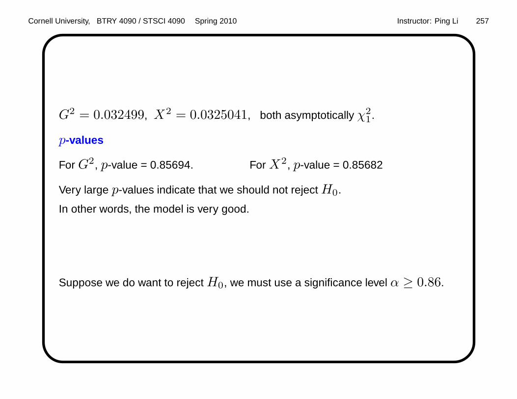
Cornell University, BTRY 4090 / STSCI 4090 Spring 2010 Instructor: Ping Li 257
G2 = 0.032499, X2 = 0.0325041, both asymptotically χ21.
p-values
For G2, p-value = 0.85694. For X2, p-value = 0.85682
Very large p-values indicate that we should not rejectH0.
In other words, the model is very good.
Suppose we do want to reject H0, we must use a significance level α ≥ 0.86.

Cornell University, BTRY 4090 / STSCI 4090 Spring 2010 Instructor: Ping Li 258
The Poisson Dispersion Test
AssumeX ∼ Poi(λ), then E(X) = λ and V ar(X) = λ.
However, for many real data, the variance may considerably exceed the mean.
Over-dispersion is often caused by subject heterogeneity, which may require a
more flexible model to explain the data
Given counts x1, ..., xn, consider
ω0 : xi ∼ Poi(λ), i = 1, 2, ..., n
Ω : xi ∼ Poi(λi), i = 1, 2, ..., n

Cornell University, BTRY 4090 / STSCI 4090 Spring 2010 Instructor: Ping Li 259
Given counts x1, ..., xn, consider
ω0 : xi ∼ Poi(λ), i = 1, 2, ..., n
Ω : xi ∼ Poi(λi), i = 1, 2, ..., n
Under ω0, the MLE is λ = x.
Λ =
maxλ∈ω0
lik(λ)
maxλi∈Ω
lik(λi)=
∏ni=1 λ
xie−λ/xi!∏n
i=1 λxii e
−λi/xi!
=
∏ni=1 x
xie−x/xi!∏n
i=1 xxi
i e−xi/xi!
=n∏
i=1
(
x
xi
)xi
exi−x
−2 log Λ = 2n∑
i=1
xi logxi
x∼ χ2
n−1 (asymptotically)

Cornell University, BTRY 4090 / STSCI 4090 Spring 2010 Instructor: Ping Li 260
Tests for Normality
If X ∼ N(µ, σ2), then
• The density function is symmetric about µ, with coefficient of skewness
b1 = 0, where
b1 =E(X − µ)3
σ3
• The coefficient of kurtosis b2 = 3, where
b2 =E(X − µ)4
σ4
These provide two simple tests for normality (among many tests).

Cornell University, BTRY 4090 / STSCI 4090 Spring 2010 Instructor: Ping Li 261
Two simple tests for normality
• Reject if the empirical coefficient of skewness |b1| is large, where
b1 =1n
∑ni=1(Xi − X)3
[
1n
∑ni=1(Xi − X)2
]3/2
• Reject if the empirical coefficient of kurtosis |b2 − 3| is large, where
b2 =1n
∑ni=1(Xi − X)4
[
1n
∑ni=1(Xi − X)2
]2
Difficulty : The distributions of b1 and b2 have no closed-forms and one must
resort to a numerical procedure.

Cornell University, BTRY 4090 / STSCI 4090 Spring 2010 Instructor: Ping Li 262
Chapter 11: Comparing Two Samples
• Comparing two independent samples
For example, a sample X1, ... , Xn is drawn from N(µX , σ2); and an
independent sample Y1, ..., Ym is drawn from N(µY , σ2).
H0 : µX = µY
HA : µY 6= µY
• Comparing paired samples
For example, we observe pairs (Xi, Yi), i = 1 to n. We would like to test
the differenceX and Y .
Pairing causes samples to be dependent, i.e., Cov(Xi, Yi) = σXY .

Cornell University, BTRY 4090 / STSCI 4090 Spring 2010 Instructor: Ping Li 263
Section 11.2: Comparing Two Independent Samples
Example: In a medical study, a sample of subjects may be assigned to a
particular treatment, and another independent sample may be assigned to a
control treatment.
• Methods based on the normal distribution
• The analysis of power

Cornell University, BTRY 4090 / STSCI 4090 Spring 2010 Instructor: Ping Li 264
Methods Based on the Normal Distribution
A sample X1, ... , Xn is drawn from N(µX , σ2);
An independent sample Y1, ..., Ym is drawn from N(µY , σ2).
The goal is to study the difference µX − µY from the observations.
By the independence assumption,
X − Y ∼ N
[
µX − µY , σ2
(
1
n+
1
m
)]
.
Two scenarios:
• σ2 is known.
• σ2 is unknown.

Cornell University, BTRY 4090 / STSCI 4090 Spring 2010 Instructor: Ping Li 265
Two Independent Normal Samples with Known Variance
X − Y ∼ N
[
µX − µY , σ2
(
1
n+
1
m
)]
.
Assume σ2 is known. Then
Z =(X − Y ) − (µX − µY )
σ√
1n + 1
m
∼ N(0, 1)
The 100(1 − α)% confidence interval of is
(X − Y ) ± zα/2 σ
√
1
n+
1
m
However, σ2 in general must be estimated from the data.

Cornell University, BTRY 4090 / STSCI 4090 Spring 2010 Instructor: Ping Li 266
Two Independent Normal Samples with Unknown Variance
The pooled sample variance
s2p =(n− 1)s2X + (m− 1)s2Y
m+ n− 2
is an estimate of the common variance σ2, where
s2X =1
n− 1
n∑
i=1
(Xi − X)2
s2Y =1
m− 1
m∑
i=1
(Yi − Y )2
are the sample variances of the X ’s and Y ’s.
s2p is the weighted average of s2X and s2Y .

Cornell University, BTRY 4090 / STSCI 4090 Spring 2010 Instructor: Ping Li 267
Theorem 11.2.A: The test statistic
t =(X − Y ) − (µX − µY )
sp
√
1n + 1
m
∼ tm+n−2
a t distribution with m+ n− 2 degrees of freedom.
Proof: Recall in Chapter 6, if V ∼ χ2n, U ∼ N(0, 1), and U and V are
independent, then U√V/n
∼ tn.

Cornell University, BTRY 4090 / STSCI 4090 Spring 2010 Instructor: Ping Li 268
s2p(m+ n− 2)
σ2=
(n− 1)s2X + (m− 1)s2Yσ2
∼ χ2m+n−2
Let
U =(X − Y ) − (µX − µY )
σ√
1n + 1
m
∼ N(0, 1)
Then
U√
s2p/σ2∼ tm+n−2
That is,
U
s2p/σ2
=
(X−Y )−(µX−µY )
σ√
1n + 1
m
sp/σ=
(X − Y ) − (µX − µY )
sp
√
1n + 1
m
∼ tm+n−2

Cornell University, BTRY 4090 / STSCI 4090 Spring 2010 Instructor: Ping Li 269
Three Types of Hypothesis Testing
The null hypothesis:
H0 : µX = µY
Three common alternative hypotheses
H1 : µX 6= µY
H2 : µX > µY
H3 : µX < µY
H1 is a two-sided alternative
H2 andH3 are one-sided alternatives

Cornell University, BTRY 4090 / STSCI 4090 Spring 2010 Instructor: Ping Li 270
Using the test statistic t = X−Y
sp
√1n + 1
m
, the rejection regions are
For H1 : |t| > tn+m−2,α/2
For H2 : t > tn+m−2,α
For H3 : t < −tn+m−2,α
Pay attention to the p-value calculation for H1.

Cornell University, BTRY 4090 / STSCI 4090 Spring 2010 Instructor: Ping Li 271
The Equivalence between t-test and Likelihood Ratio Test
H0 : µX = µY , H1 : µX 6= µY .
Three parameters: θ =(
µX , µY , σ2)
.
Λ =
maxθ∈ω0
lik(µX , µY , σ2)
maxθ∈Ω
lik(µX , µY , σ2)
We can show rejecting small Λ (i.e., rejecting large −2 log Λ) is equivalent to
rejecting large |t| = |X−Y |sp
√1n + 1
m
.

Cornell University, BTRY 4090 / STSCI 4090 Spring 2010 Instructor: Ping Li 272
Three parameters: θ =(
µX , µY , σ2)
.
ω0 = µX = µY = µ0, 0 < σ = σ0 <∞Ω = −∞ < µX , µY <∞, 0 < σ <∞
lik(µX , µY , σ2)
=n∏
i=1
1√2πσ
exp
[
− (Xi − µX)2
2σ2
] m∏
i=1
1√2πσ
exp
[
− (Yi − µY )2
2σ2
]
l(µX , µY , σ2) = − m+ n
2log 2π − m+ n
2log σ2
− 1
2σ2
[
n∑
i=1
(Xi − µX)2 +m∑
i=1
(Yi − µY )2
]

Cornell University, BTRY 4090 / STSCI 4090 Spring 2010 Instructor: Ping Li 273
Under ω0 = µX = µY = µ0, 0 < σ = σ0 <∞
l(µ0, σ20) = − m+ n
2log 2π − m+ n
2log σ2
0
− 1
2σ20
[
n∑
i=1
(Xi − µ0)2 +
m∑
i=1
(Yi − µ0)2
]
In fact, since both Xi ∼ N(µ0, σ20) and Yi ∼ N(µ0, σ
20), Xi and Yi are
independent, we have m+ n samples in N(µ0, σ20).
Therefore, the MLEs are
µ0 =1
m+ n
[
n∑
i=1
Xi +m∑
i=1
Yi
]
=n
m+ nX +
m
m+ nY
σ20 =
1
m+ n
[
n∑
i=1
(Xi − µ0)2 +
m∑
i=1
(Yi − µ0)2
]

Cornell University, BTRY 4090 / STSCI 4090 Spring 2010 Instructor: Ping Li 274
Thus, under the null ω0 = µX = µY = µ0, 0 < σ = σ0 <∞
l(µ0, σ20) = − m+ n
2log 2π − m+ n
2log σ2
0 − m+ n
2
Under Ω = −∞ < µX , µY <∞, 0 < σ <∞. We can show
µX = X, µY = Y
σ2 =1
m+ n
[
n∑
i=1
(Xi − µX)2 +m∑
i=1
(Yi − µY )2
]
l(µX , µY , σ2) = −m+ n
2log 2π − m+ n
2log σ2 − m+ n
2

Cornell University, BTRY 4090 / STSCI 4090 Spring 2010 Instructor: Ping Li 275
The negative log likelihood ratio is
−[
l(µ0, σ20) − l(µX , µY , σ
2)]
=m+ n
2log
σ20
σ2
Therefore, the test rejects for large values ofσ20
σ2 .
σ20
σ2=
∑ni=1(Xi − µ0)
2 +∑n
i=1(Yi − µ0)2
∑ni=1(Xi − X)2 +
∑ni=1(Yi − Y )2
=1 +mn
m+ n
(X − Y )2∑n
i=1(Xi − X)2 +∑n
i=1(Yi − Y )2
Equivalently, the test rejects for large values of
|X − Y |√
∑ni=1(Xi − X)2 +
∑ni=1(Yi − Y )2
which is the t statistic.

Cornell University, BTRY 4090 / STSCI 4090 Spring 2010 Instructor: Ping Li 276
Power Analysis of Two-Sample t Test
Recall power = 1 - Type II error = P (rejectH0|HA).
To compute the power, we must specify a simple alternative hypothesis. We
consider
H0 : µX − µY = 0
H1 : µX − µY = ∆.
For simplicity, we assume σ2 is known and n = m.
The t test rejects if |X − Y | > zα/2σ√
2n .

Cornell University, BTRY 4090 / STSCI 4090 Spring 2010 Instructor: Ping Li 277
power =P
(
|X − Y | > zα/2σ
√
2
n|H1
)
=P
(
X − Y > zα/2σ
√
2
n|H1
)
+ P
(
X − Y < −zα/2σ
√
2
n|H1
)
Note that X − Y |H1 ∼ N(
µX − µY = ∆, 2σ2
n
)
. Therefore,
P
(
X − Y > zα/2σ
√
2
n|H1
)
=P
X − Y − ∆
σ√
2/n>zα/2σ
√
2n − ∆
σ√
2/n|H1
=1 − Φ
[
zα/2 −∆
σ
√
n/2
]

Cornell University, BTRY 4090 / STSCI 4090 Spring 2010 Instructor: Ping Li 278
Therefore, the power can be computed from
power =1 − Φ
[
zα/2 −∆
σ
√
n/2
]
+ Φ
[
−zα/2 −∆
σ
√
n/2
]
=1 − Φ[
zα/2 − ∆′]+ Φ[
−zα/2 − ∆′]
where ∆′ = ∆σ
√
n/2.
Three parameters, α, ∆, and n, affect the power.
• Larger α =⇒ smaller zα/2 =⇒ larger power.
• Larger |∆′| =⇒ larger power.
• Larger |∆| =⇒ larger power.
• Larger n =⇒ larger power.
• Smaller σ =⇒ larger power.
What is the relation between α and power if ∆ = 0?

Cornell University, BTRY 4090 / STSCI 4090 Spring 2010 Instructor: Ping Li 279
Section 11.3: Comparing Paired Samples
In many cases, the samples are paired (and dependent),
for example, measurements before and after medical treatments.
Consider
(Xi, Yi), i = 1, 2, ...n
(Xi, Yi) is independent of (Xj , Yj), if i 6= j
E(Xi) = µX , E(Yi) = µY
V ar(Xi) = σ2X , V ar(Yi) = σ2
Y

Cornell University, BTRY 4090 / STSCI 4090 Spring 2010 Instructor: Ping Li 280
Let Di = Xi − Yi, and D = 1n
∑ni=1Di. Then,
E(D) = µX − µY ,
V ar(D) =1
n
(
σ2X + σ2
Y − 2ρσXσY
)
Therefore, D is still an unbiased estimator of µX − µY , but it has smaller
variance if there exists positive correlation (ρ > 0).

Cornell University, BTRY 4090 / STSCI 4090 Spring 2010 Instructor: Ping Li 281
Paired Test Based on the Normal Distribution
This methods assume that Di = Xi − Yi is i.i.d. normal with
E(Di) = µD, V ar(Di) = σ2D
In general, σ2D needs to be estimated from the data.
Consider a two-sided test
H0 : µD = 0, HA : µD 6= 0
A t-test rejects for large values of |t|, where t = D−µD
sD.
The rejection region is D > tn−1,α/2sD.

Cornell University, BTRY 4090 / STSCI 4090 Spring 2010 Instructor: Ping Li 282
Example 11.3.1.A: Effect of cigarette smoking on platelet aggregation.
Before (X) After (Y ) Difference (D)
25 27 2
25 29 4
27 37 10
44 56 12
30 46 16
67 82 15
53 57 4
53 80 27
52 61 9
60 59 -1
28 43 15

Cornell University, BTRY 4090 / STSCI 4090 Spring 2010 Instructor: Ping Li 283
D = 10.272
sD =
√
63.6182
11= 2.405
ρ = 0.8938
H0 : t =D
sD
=10.272
2.405= 4.271.
Suppose α = 0.01.
tα/2,n−1 = t0.005,10 = 3.169 < t.
Therefore, the test rejects H0 at significance level α = 0.01.
Alternatively, we say the p-value is smaller than 0.01.

Cornell University, BTRY 4090 / STSCI 4090 Spring 2010 Instructor: Ping Li 284
A Heuristic Explanation on GLRT
Why, underH0, the test statistic
Λ =
maxθ∈ω0
lik(θ)
maxθ∈Ω
lik(θ)
satisfies
−2 log Λ → χ2s, as n→ ∞??
The heuristic argument
• Only considers s = 1.
• Utilizes Taylor expansion.
• Uses the fact that the MLE is asymptotically normal.

Cornell University, BTRY 4090 / STSCI 4090 Spring 2010 Instructor: Ping Li 285
Since s = 1, we considerH0 : θ = θ0.
Let l(θ) = log lik(θ) and θ be the MLE of θ ∈ Ω.
−2 log Λ = −2[
l(θ0) − l(θ)]
Applying Taylor expansion
l(θ0) = l(θ) + (θ0 − θ)l′(θ) +(θ0 − θ)2
2l′′(θ) + ...
Because θ is the MLE, we know l′(θ) = 0. Therefore,
−2 log Λ = −2[
l(θ0) − l(θ)]
= −l′′(θ)(θ0 − θ)2 + ...

Cornell University, BTRY 4090 / STSCI 4090 Spring 2010 Instructor: Ping Li 286
The MLE is asymptotically normal, i.e., as n→ ∞,(
θ − θ0
)
√
1nI(θ)
=(
θ − θ0
)
√
nI(θ) → N(0, 1)
Because nI(θ) = −E(l′′(θ)), we can (heuristically) write, as n→ ∞,
−2 log Λ = − l′′(θ)(θ0 − θ)2
≈[(
θ − θ0
)
√
nI(θ)]2
→χ21
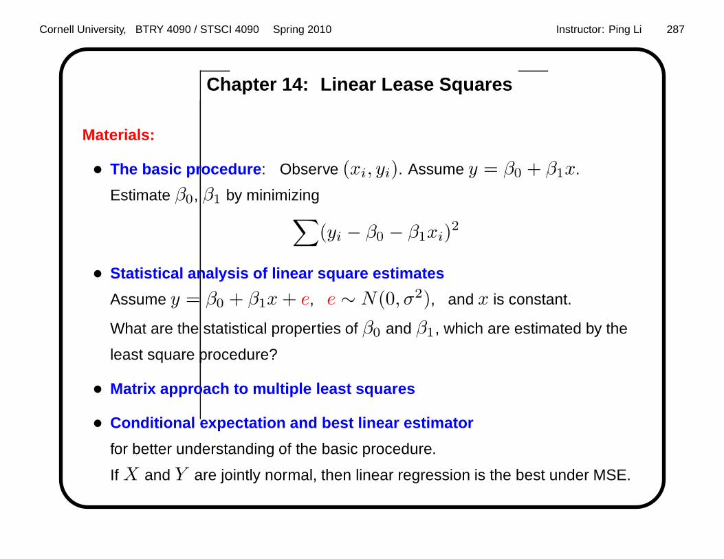
Cornell University, BTRY 4090 / STSCI 4090 Spring 2010 Instructor: Ping Li 287
Chapter 14: Linear Lease Squares
Materials:
• The basic procedure : Observe (xi, yi). Assume y = β0 + β1x.
Estimate β0, β1 by minimizing∑
(yi − β0 − β1xi)2
• Statistical analysis of linear square estimates
Assume y = β0 + β1x+ e, e ∼ N(0, σ2), and x is constant.
What are the statistical properties of β0 and β1, which are estimated by the
least square procedure?
• Matrix approach to multiple least squares
• Conditional expectation and best linear estimator
for better understanding of the basic procedure.
If X and Y are jointly normal, then linear regression is the best under MSE.

Cornell University, BTRY 4090 / STSCI 4090 Spring 2010 Instructor: Ping Li 288
Linear Lease Squares: The Basic Procedure
The basic procedure is to fit a straight line to a plot of points (xi, yi),
y = β0 + β1x
by minimizing
L(β0, β1) =n∑
i=1
(yi − β0 − β1xi)2,
i.e., solving for β0 and β1 from
∂L(β0, β1)
∂β0= 0
∂L(β0, β1)
∂β1= 0

Cornell University, BTRY 4090 / STSCI 4090 Spring 2010 Instructor: Ping Li 289
Taking the first derivatives,
∂L(β0, β1)
∂β0=
n∑
i=1
2(yi − β0 − β1xi)(−1)
∂L(β0, β1)
∂β1=
n∑
i=1
2(yi − β0 − β1xi)(−xi)
Setting them to zero =⇒
β0 =y − xβ1
β1 =
∑ni=1 xiyi − y
∑ni=1 xi
∑ni=1 x
2i − x
∑ni=1 xi

Cornell University, BTRY 4090 / STSCI 4090 Spring 2010 Instructor: Ping Li 290
Statistical Properties of β0 and β1
Model:
yi = β0 + β1xi + ei, i = 1, 2, ..., n
ei ∼ N(0, σ2), i.i.d.
xi’s are constants. The randomness of yi’s is due to ei.
The coefficients β0 and β1 are estimated by least squares.
Q: Under this model, what are E(β0), V ar(β0), E(β1), V ar(β1), etc.?

Cornell University, BTRY 4090 / STSCI 4090 Spring 2010 Instructor: Ping Li 291
According to the model: yi = β0 + β1xi + ei, ei ∼ N(0, σ2),
E(yi) = β0 + β1xi
E(y) = β0 + β1x
V ar(yi) = σ2
Cov(yi, yj) = 0, if i 6= j
Therefore,
E(β0) = E(y − xβ1) = β0 + β1x− xE(β1)
i.e., E(β0) = β0 iff E(β1) = β1

Cornell University, BTRY 4090 / STSCI 4090 Spring 2010 Instructor: Ping Li 292
E(β1) =E
[∑ni=1 xiyi − y
∑ni=1 xi
∑ni=1 x
2i − x
∑ni=1 xi
]
=
∑ni=1 xiE(yi) −E(y)
∑ni=1 xi
∑ni=1 x
2i − x
∑ni=1 xi
=
∑ni=1 xi (β0 + β1xi) − (β0 + β1x)
∑ni=1 xi
∑ni=1 x
2i − x
∑ni=1 xi
=β1
∑ni=1 x
2i − β1x
∑ni=1 xi
∑ni=1 x
2i − x
∑ni=1 xi
=β1
Theorem 14.2.A: Unbiasedness
E(β0) = β0, E(β1) = β1

Cornell University, BTRY 4090 / STSCI 4090 Spring 2010 Instructor: Ping Li 293
Another way to express β1:
β1 =
∑ni=1 xiyi − y
∑ni=1 xi
∑ni=1 x
2i − x
∑ni=1 xi
=
∑ni=1(xi − x)(yi − y)∑n
i=1(xi − x)2
=
∑ni=1(xi − x)yi
∑ni=1(xi − x)2
Note that
n∑
i=1
(xi − x) = 0,n∑
i=1
(yi − y) = 0.
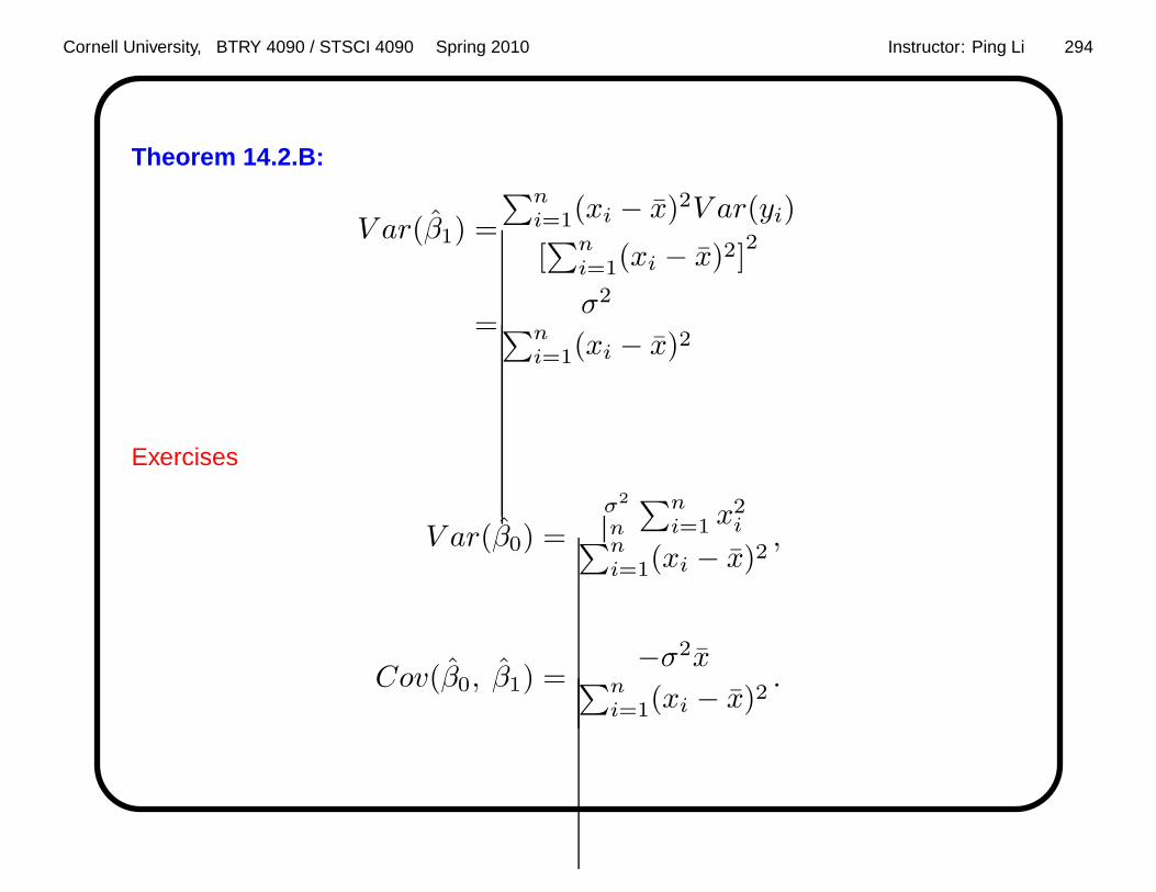
Cornell University, BTRY 4090 / STSCI 4090 Spring 2010 Instructor: Ping Li 294
Theorem 14.2.B:
V ar(β1) =
∑ni=1(xi − x)2V ar(yi)
[∑n
i=1(xi − x)2]2
=σ2
∑ni=1(xi − x)2
Exercises
V ar(β0) =σ2
n
∑ni=1 x
2i
∑ni=1(xi − x)2
,
Cov(β0, β1) =−σ2x
∑ni=1(xi − x)2
.

Cornell University, BTRY 4090 / STSCI 4090 Spring 2010 Instructor: Ping Li 295
Residual Sum of Squares (RSS)
Definition
RSS =n∑
i=1
(yi − β0 − β1xi)2
We can show
E(RSS) = (n− 2)σ2
In other words,
s2 =RSS
n− 2
is an unbiased estimator of σ2.

Cornell University, BTRY 4090 / STSCI 4090 Spring 2010 Instructor: Ping Li 296
E(RSS) = E
[
n∑
i=1
(yi − β0 − β1xi)2
]
=E
[
n∑
i=1
(β0 + β1xi + ei − β0 − β1xi)2
]
=E
[
n∑
i=1
(β0 − β0 + (β1 − β1)xi + ei)2
]
=nV ar(β0) + V ar(β1)n∑
i=1
x2i + nσ2 + 2Cov(β0, β1)
n∑
i=1
xi
+ 2E
[
n∑
i=1
ei
(
β0 − β0 + (β1 − β1)xi
)
]
=(n+ 2)σ2 + 2E
[
n∑
i=1
ei
(
β0 − β0 + (β1 − β1)xi
)
]

Cornell University, BTRY 4090 / STSCI 4090 Spring 2010 Instructor: Ping Li 297
E
[
n∑
i=1
ei
(
β0 − β0 + (β1 − β1)xi
)
]
=E
[
n∑
i=1
ei
(
β0 − y + xβ1 + (β1 − β1)xi
)
]
=E
[
n∑
i=1
ei
(
β0 − β0 − xβ1 − e+ xβ1 + (β1 − β1)xi
)
]
=E
[
n∑
i=1
ei
(
−xβ1 + xβ1 + (β1 − β1)xi
)
]
− σ2
=E
[
β1
n∑
i=1
ei (x− xi)
]
− σ2

Cornell University, BTRY 4090 / STSCI 4090 Spring 2010 Instructor: Ping Li 298
E
[
β1
n∑
i=1
ei (x− xi)
]
=E
[
∑ni=1(xi − x)yi
∑ni=1(xi − x)2
n∑
i=1
ei (x− xi)
]
=E
[
∑ni=1(xi − x)(β0 + β1xi + ei)
∑ni=1(xi − x)2
n∑
i=1
ei (x− xi)
]
=E
[∑ni=1(xi − x)(x− xi)e
2i
∑ni=1(xi − x)2
]
= − σ2
Therefore,
E(RSS) = (n+ 2)σ2 + 2(−2σ2) = (n− 2)σ2

Cornell University, BTRY 4090 / STSCI 4090 Spring 2010 Instructor: Ping Li 299
The Distributions β0 and β1
Model: yi = β0 + β1xi + ei, ei ∼ N(0, σ2),
yi ∼ N(β0 + β1xi, σ2)
β1 =
n∑
i=1
ciyi ∼ N(β1, V ar(β1))
β0 = y − xβ1 ∼ N(β0, V ar(β0))
s2
σ2(n− 2) =
RSS
σ2∼ χ2
n−2
β0 − β0
sβ0
∼ tn−2,β1 − β1
sβ1
∼ tn−2
What if ei is not normal? Central limit theorem and normal approximation.

Cornell University, BTRY 4090 / STSCI 4090 Spring 2010 Instructor: Ping Li 300
Hypothesis Testing
Once we know the distributions
β0 − β0
sβ0
∼ tn−2,β1 − β1
sβ1
∼ tn−2
we can conduct hypothesis test, for example,
H0 : β1 = 0
HA : β1 6= 0

Cornell University, BTRY 4090 / STSCI 4090 Spring 2010 Instructor: Ping Li 301
Multiple Least Squares
Model: yi = β0 + β1xi,1 + ...+ βp−1xi,p−1 + ei, ei ∼ N(0, σ2) i.i.d.
Observations: (xi, yi), i = 1 to n.
Multiple least squares : Estimate βj by minimizing the MSE
L(βj , j = 0, 1, ..., p− 1) =
n∑
i=1
(yi − β0 −p−1∑
j=1
xi,jβj)2

Cornell University, BTRY 4090 / STSCI 4090 Spring 2010 Instructor: Ping Li 302
Matrix Approach to Linear Least Square
X =
1 x1,1 x1,2 . . . x1,p−1
1 x2,1 x2,2 . . . x2,p−1
1 x3,1 x3,2 . . . x3,p−1
......
......
...
1 xn,1 xn,2 . . . xn,p−1
, β =
β0
β1
β2
...
βp−1
L(β) =n∑
i=1
(yi − β0 −p−1∑
j=1
xi,jβj)2 = ‖Y − Xβ‖2

Cornell University, BTRY 4090 / STSCI 4090 Spring 2010 Instructor: Ping Li 303
L(β) =
n∑
i=1
(yi − β0 −p−1∑
j=1
xi,jβj)2 = ‖Y − Xβ‖2
Matrix/vector derivative
∂L(β)
∂β=2(−XT) (Y − Xβ)
= − 2(
XTY − XTXβ)
= 0
=⇒
XTXβ = XTY
=⇒β =[
XTX]−1
XTY

Cornell University, BTRY 4090 / STSCI 4090 Spring 2010 Instructor: Ping Li 304
Statistical Properties of β
Model:
Y = Xβ + e, ei ∼ N(0, σ)2 i.i.d.
Unbiasedness (Theorem 14.4.2.A):
Eβ =E(
[
XTX]−1
XTY)
=E(
[
XTX]−1
XT [Xβ + e])
=E(
[
XTX]−1 [
XTX]
β)
+ E(
[
XTX]−1
XTe)
=β

Cornell University, BTRY 4090 / STSCI 4090 Spring 2010 Instructor: Ping Li 305
Covariance matrix of β (Theorem 14.4.2.B)
V ar(
β)
=V ar(
[
XTX]−1 [
XTX]
β +[
XTX]−1
XTe)
=V ar(
[
XTX]−1
XTe)
=[
XTX]−1
XT V ar(e)[
[
XTX]−1
XT]T
=[
XTX]−1
XT V ar(e) X[
XTX]−1
=σ2[
XTX]−1
XTX[
XTX]−1
=σ2[
XTX]−1
Note that V ar(e) is a diagonal matrix = σ2In×n

Cornell University, BTRY 4090 / STSCI 4090 Spring 2010 Instructor: Ping Li 306
Theorem 14.4.3.A: An unbiased estimator of σ2 is s2, where
s2 =‖Y − Y‖2
n− p
Proof:
Y = Xβ =[
X[
XTX]−1
XT]
Y = PY
Lemma 14.4.3.A :
P2 = P = PT
(I − P)2 = I − P = (I− P)T
Proof of Lemma 14.4.3.A
P2 = X[
XTX]−1
XT X[
XTX]−1
XT = X[
XTX]−1
XT = P

Cornell University, BTRY 4090 / STSCI 4090 Spring 2010 Instructor: Ping Li 307
Therefore,
‖Y − Y‖2 = ‖(I− P)Y‖2 = YT(I− P)T(I− P)Y = YT(I− P)Y
and
E[
YT(I− P)Y]
=E[(
βTXT + eT)
(I− P) (Xβ + e)]
=βTXT(I− P)Xβ +E[
eT(I − P)e]
=E[
eT(I− P)e]
=nσ2 −E[
eTPe]
because
XT(I− P)X = XTX − XT[
X[
XTX]−1
XT]
X = 0

Cornell University, BTRY 4090 / STSCI 4090 Spring 2010 Instructor: Ping Li 308
E[
eT(P)e]
=E
p∑
j=1
[
n∑
i=1
eiPij
]
ej
=E
p∑
j=1
Pjje2j
=σ2
p∑
j=1
Pjj = pσ2
where we skip the proof of the very last step.
Combining the results, we obtain
E(
‖Y − Y‖2)
= (n− p)σ2

Cornell University, BTRY 4090 / STSCI 4090 Spring 2010 Instructor: Ping Li 309
Properties of Residuals
Residuals: e = Y − Y = (I− P)Y.
Covariance matrix of residuals:
V ar(e) =(I− P)Var(Y)(I− P)T
=(I− P)σ2I(I − P)
=σ2(I− P)
=⇒ Residuals are correlated

Cornell University, BTRY 4090 / STSCI 4090 Spring 2010 Instructor: Ping Li 310
Theorem 14.4.A: The residuals are uncorrelated with the fitted values.
Proof:
E(eTY) =E(
YT(I− P)PY)
=E(
YT(P − P2)Y)
=E(
YT(P − P)Y)
=0

Cornell University, BTRY 4090 / STSCI 4090 Spring 2010 Instructor: Ping Li 311
Inference about β
V ar(
β)
= σ2[
XTX]−1
= σ2C.
Using s2 to estimate σ2, we obtain the distribution
βj − βj
sβj
∼ tn−p, where sβj= s
√cii
which allows us to conduct hypothesis test on the significance of the fit.