Interpreting breakeven and profit volume charts - ACCA · PDF fileInterpreting breakeven and profit
description
Bruno Dupire
Bloomberg LP
Lecture 9Volatility

Bruno Dupire 2
Forward Equations (1)
• BWD Equation: price of one option for different
• FWD Equation: price of all options for current
• Advantage of FWD equation:– If local volatilities known, fast computation of implied
volatility surface,– If current implied volatility surface known, extraction of
local volatilities,– Understanding of forward volatilities and how to lock
them.
( )tS ,
( )00 , tS( )TKC ,
( )00 ,TKC

Bruno Dupire 3
Forward Equations (2)
• Several ways to obtain them:– Fokker-Planck equation:
• Integrate twice Kolmogorov Forward Equation– Tanaka formula:
• Expectation of local time– Replication
• Replication portfolio gives a much more financial insight

Bruno Dupire 4
Fokker-Planck
• If• Fokker-Planck Equation:
• Where is the Risk Neutral density. As
• Integrating twice w.r.t. x:
( )dWtxbdx ,= ( )2
22
21
xb
t ∂∂
=∂∂ ϕϕ
2
2
KC
∂∂
=ϕϕ
2
2
222
2
2
2
2
21
xKCb
tKC
xtC
∂
∂∂
∂=
∂
∂∂
∂=
∂
∂∂
∂
2
22
2 KCb
tC
∂∂
=∂∂

Bruno Dupire 5
FWD Equation: dS/S = σ(S,t) dW
TCC
CS TKTTKTTK δ
δδ ,,, Define
−≡ +
TTKC δ+,TKC , ST
K
dT
dT/2
Tat ,T
TKCS δ
ST
K
0→Tδ
ST
K
( )TKKTK,
22
2, δσ
( )2
22
2
2,
KCKTK
TC
∂∂
=∂∂ σEquating prices at t0:

Bruno Dupire 6
FWD Equation: dS/S = r dt + σ(S,t) dW
= Tat ,T
TKCS δ
( )KCrK
KCKTK
TC
∂∂
−∂∂
=∂∂
2
22
2
2,σ
Time Value + Intrinsic Value(Strike Convexity) (Interest on Strike)
Equating prices at t0:
TV IV
TrKe δ− K
rK
ST
TTKC δ+,
TrKe δ− K ST
TKC ,
TV IVTr
T KeS δ−−
KST −
0→TδTKrKDig ,
K ST
( )TKKTK,
22
2, δσ

Bruno Dupire 7
FWD Equation: dS/S = (r-d) dt + σ(S,t) dW
= Tat ,T
TKCS δ
TrdKe δ)( − K( )Kdr −
ST
0→Tδ
TKDigKdr , )( −
( )TKKTK,
22
2, δσ
K ST
TKCd ,⋅− TKCd ,⋅−
TTKC δ+,
( ) TrdKe δ− KST
TKC ,
TVIV
TrTdT KeeS δδ −− −
TrT KeS δ−−
TV + Interests on K – Dividends on S
( ) ( ) CdKCKdr
KCKTK
TC
⋅−∂∂
−−∂∂
=∂∂
2
22
2
2,σEquating prices at t0:

Bruno Dupire 8
Stripping Formula
– If known, quick computation of all today,
– If all known:
Local volatilities extracted from vanilla pricesand used to price exotics.
( )TK ,σ
( ) ( ) CdKCKdr
KCKTK
TC
⋅−∂∂
−−∂∂
=∂∂
2
222
2,σ
( )00, , tSC TK
( )( )
2
22
2,
KCK
dCKCKdr
TC
TK
∂∂
+∂∂
−+∂∂
=σ
( )00, ,tSC TK

Bruno Dupire 9
Smile dynamics: Local Vol Model (1)
• Consider, for one maturity, the smiles associated to 3 initial spot values
Skew case
– ATM short term implied follows the local vols– Similar skews
+S0S−S
Local vols
−S Smile
0 Smile S+S Smile
K

Bruno Dupire 10
Smile dynamics: Local Vol Model (2)
• Pure Smile case
– ATM short term implied follows the local vols– Skew can change sign
K−S 0S +S
Local vols
−S Smile
0 Smile S
+S Smile

Bruno Dupire 11
Summary of LVM Properties
is the initial volatility surface
• compatible with local vol
• compatible with = (local vol)²
• deterministic function of (S,t)
future smile = FWD smile from local vol
( )tS,σ =⇔Σ σ0
Tk,σ̂
( )ωσ [ ]KSE T =⇔Σ 20 σ
⇔
0Σ

Volatility Replication

Bruno Dupire 13
Volatility Replication
dWS
dStσ= Apply Ito to f(S,t).
−−−=⇒
++=
∫ ∫∫T T
ttSttT
T
ttSS
tSStS
dStSfdttSfSfTSfdtStSf
dtSfdtfdSfdf
0 00
2
0
2
2221
),(),()0,(),(2),( σ
σ
European PF ∆-hedge
∫∫== 22 :),(),(
SgfStSftSg SSdttSg t∫ 2),( σTo replicate ,find f :
T
0

Bruno Dupire 14
Examples
Local Time at level K
Absolute Variance Swap
FWD Variance Swap
Corridor Variance Swap
Variance Swap
)(1),( ],[ 21ttSg TT=
)ln(),(0S
StSf −=
)ln(),(0S
StSf −= on [a,b]
+ linear extrapolation
1),( =tSg
)(1),( ],[ tba StSg =
)(1)ln(),( ],[0
21t
SStSf TT×−=
2)(),(
20SStSf −
=2),( StSg =
2
)(),(K
KStSf+−
=)(),( StSg Kδ=

Bruno Dupire 15
Conditional Instantaneous FWD Variance
20
2 ),(2)(K
TKCdtSET
Kt ×=
∫ δσ
[ ] [ ] [ ] ),(2)()( 222 TK
TC
KSEKSESE TKTTTKT ∂
∂×=⋅== δσδσ
From local time:
Differentiating wrt T:
And, as: [ ] ),()( 2
2
TKKCSE TK ∂
∂=δ
[ ] ),(),(
),(2 2
2
222 TK
TKKC
TKTC
KKSE locTT σσ =
∂∂∂∂
×==

Bruno Dupire 16
Deterministic future smiles
S0
K
ϕ
T1 T2t0
It is not possible to prescribe just any future smileIf deterministic, one must have
Not satisfied in general( ) ( ) ( )dSTSCTStStSC TKTK 1,10000, ,,,,,
22 ∫= ϕ

Bruno Dupire 17
Det. Fut. smiles & no jumps => = FWD smile
If
stripped from SmileS.t
Then, there exists a 2 step arbitrage:Define
At t0 : Sell
At t:
gives a premium = PLt at t, no loss at T
Conclusion: independent of from initial smile
( ) ( ) ( ) ( )TTKKTKTKtSVTKtS impTKTK δδσσ
δδ
++≡≠∃→→
,,,lim,,/,,, 2
00
2,
( ) ( )( ) ( )TKtSKCtSVTKPL TKt ,,,,, 2
2
,2
∂∂
−≡ σ
( )tStSt DigDigPL ,, εε +− −⋅S
t0 t T
S0
K
[ ] ( ) TKt TKK
SSS ,2
TK,2 , sell , CS2buy , if δσεε +−∈
( ) ( ) ( )TKtSVtS TK ,,, 200, σ==( )tSV TK ,,

Bruno Dupire 18
Consequence of det. future smiles
• Sticky Strike assumption: Each (K,T) has a fixed independent of (S,t)
• Sticky Delta assumption: depends only on moneyness and residual maturity
• In the absence of jumps,– Sticky Strike is arbitrageable– Sticky ∆ is (even more) arbitrageable
),( TKimplσ
),( TKimplσ

Bruno Dupire 19
Example of arbitrage with Sticky Strike
21CΓ
12CΓ
1tS
ttS δ+
Each CK,T lives in its Black-Scholes ( )world
P&L of Delta hedge position over dt:
If no jump
21,2,1 assume2211
σσ >≡≡ TKTK CCCC
!
( ) ( )( )( ) ( )( )( ) ( )
( )ΘΓ
>−ΓΓ
=Γ−Γ
Γ−=
Γ−=
free , no
02
22
21
2211221
22
22
21
2
12
12
21
1
tSCCPL
tSSCPL
tSSCPL
δσσδ
δσδδ
δσδδ
),( TKimplσ

Bruno Dupire 20
Arbitraging Skew Dynamics
• In the absence of jumps, Sticky-K is arbitrageable and Sticky-∆ even more so.
• However, it seems that quiet trending market (no jumps!) are Sticky-∆.
In trending markets, buy Calls, sell Puts and ∆-hedge.
Example:tS1K
2K12 KK PCPF −≡
21,σσ
Vega > Vega2K 1K
21,σσ
Vega < Vega2K 1K
S
S P
PF
F
∆-hedged PF gains from S induced volatility moves.

Skew from Historical Prices

Bruno Dupire 22
Theoretical Skew from Prices
?
ð
Problem : How to compute option prices on an underlying without options?
For instance : compute 3 month 5% OTM Call from price history only.
1) Discounted average of the historical Intrinsic Values.
Bad : depends on bull/bear, no call/put parity.
2) Generate paths by sampling 1 day return recentered histogram.
Problem : CLT ðconverges quickly to same volatility for all strike/maturity; breaks autocorrelation and vol/spot dependency.

Bruno Dupire 23
Theoretical Skew from Prices (2)
3) Discounted average of the Intrinsic Value from recentered 3 month histogram.
4) ∆-Hedging : compute the implied volatility which makes the ∆-hedging a fair game.

Bruno Dupire 24
Theoretical Skewfrom historical prices
How to get a theoretical Skew just from spot price history?Example: 3 month daily data1 strike – a) price and delta hedge for a given within Black-Scholes
model– b) compute the associated final Profit & Loss: – c) solve for– d) repeat a) b) c) for general time period and average– e) repeat a) b) c) and d) to get the “theorical Skew”
1TSkK =σ
( )σPL( ) ( )( ) 0/ =kPLk σσ
t
S
1TS
1T 2T
K

IV. Volatility Expansion

Bruno Dupire 26
Introduction
• This talk aims at providing a betterunderstanding of:
– How local volatilities contribute to the value ofan option
– How P&L is impacted when volatility ismisspecified
– Link between implied and local volatility– Smile dynamics– Vega/gamma hedging relationship

Bruno Dupire 27
Framework & definitions
• In the following, we specify the dynamicsof the spot in absolute convention (as opposed to proportional in Black-Scholes) and assume no rates:
• : local (instantaneous) volatility(possibly stochastic)
• Implied volatility will be denoted by
dS dWt t t=σσ
$σ

Bruno Dupire 28
P&L of a delta hedged option
P&L
St t+∆
St
Θ
Break-evenpoints
σ ∆t
−σ ∆t
Option Value
St
CtCt t+ ∆
S
Delta hedge

Bruno Dupire 29
P&L of a delta hedged option (2)
P&L P&L
Expected P&L = 0 Expected P&L > 0
Correct Volatility higher than
St t+ ∆StSt t+ ∆St
Ito: When , spot dependency disappears∆t → 0
1st 1st1st 1st

Bruno Dupire 30
Black-Scholes PDE
P&L is a balance between gain from Γ and
From Black-Scholes PDE:( ) P L dtt t dt& , + = +
σ 2
0 02Γ Θ Θ Γ0
02
02= −
σ
=> discrepancy if σ different from
( )gain over dt = −12
202
0σ σ Γ dt
• >• <
σ σσ σ
0
00
::ProfitLoss
Magnified by Γ

Bruno Dupire 31
P&L over a pathTotal P&L over a path
= Sum of P&L over all small time intervals
Spot
Time
GammaP L
dtT
&
( )
=
−∫12
202
00σ σ Γ
No assumption is madeon volatility so far

Bruno Dupire 32
General case
• Terminal wealth on each path is:
( is the initial price of the option)( )X Σ0
( )wealth = T X dtT
Σ Γ02
02
00
12+ −∫ ( )σ σ
• Taking the expectation, we get:
[ ]E X E S dSdtTϕ σ σ ϕwealthT = + −
∞
∫∫( ) [ ( )| ]Σ Γ0 02
02
00
12
• The probability density φ may correspond to the density ofa NON risk-neutral process (with some drift) with volatility σ.

Bruno Dupire 33
Non Risk-Neutral world• In a complete model (like Black-Scholes), the drift doesnot affect option prices but alternative hedging strategieslead to different expectations
L
Profile of a call (L,T) for different vol assumptions
Example: mean reverting processtowards L with high volatility around L
We then want to choose K (close to L) T and σ0 (small) to take advantage of it.
In summary: gamma is a volatilitycollector and it can be shaped by:
• a choice of strike and maturity,• a choice of σ0 , our hedging volatility.

Bruno Dupire 34
Average P&L
• From now on, φ will designate the risk neutral densityassociated with .
•In this case, E[wealthT] is also and we have:
dS dWt t= σ
( )X Σ
X X E S dS dtT
( ) ( ) [ ( )| ]Σ Σ Γ= + −∞
∫∫0 02
02
00
12 σ σ ϕ
• Path dependent option & deterministic vol:
X X E S dS dt( ) ( ) ( ) [ | ]Σ Σ Γ= + −∫∫02
02
012 σ σ ϕ
• European option & stochastic vol:
C C E S dS dt( ) ( ) ( [ | ] )Σ Σ Γ= + −∫∫02
02
012 σ σ ϕ

Bruno Dupire 35
Quiz
• Buy a European option at 20% implied vol
• Realised historical vol is 25%
• Have you made money ?
Not necessarily!
High vol with low gamma, low vol with high gamma

Bruno Dupire 36
Expansion in volatility
• An important case is a European option withdeterministic vol:
C C dS dt( ) ( ) ( )Σ Σ Γ= + −∫∫02
02
012 σ σ ϕ
• The corrective term is a weighted average of the volatilitydifferences
• This double integral can be approximated numerically

Bruno Dupire 37
P&L: Stop Loss Start Gain
• Extreme case: σ δ0 00= ⇒ =Γ K
( ) ( )C S K K t K t dtT
( ) ( ) , ,Σ = − ++ ∫02
0
12 σ ϕ
• This is known as Tanaka’s formula
t
Delta = 100%K
Delta = 0%
S

Bruno Dupire 38
Local / Implied volatility relationship
13
15
17
19
21
23
Implied volatility
strike maturity
11
15
19
23
27
31
Local volatility
spot time
Aggregation
Differentiation
Bruno Dupire 39
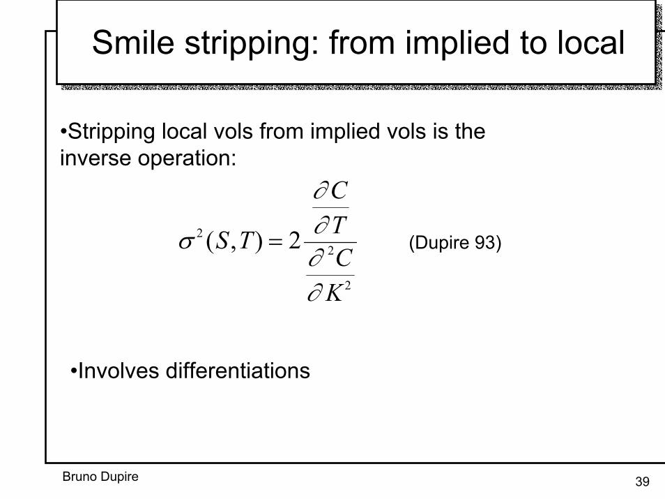
Smile stripping: from implied to local
•Stripping local vols from implied vols is theinverse operation:
σ
∂∂∂∂
22
2
2( , )S T
CTC
K
= (Dupire 93)
•Involves differentiations

Bruno Dupire 40
From local to implied: a simple case
Let us assume that local volatility is a deterministic function of time only:
( )dS t dWt t= σ
In this model, we know how to combine local vols to compute implied vol:
( )( )
$σσ
Tt dt
T
T
=∫ 2
0
Question: can we get a formula with ? ( )σ S t,
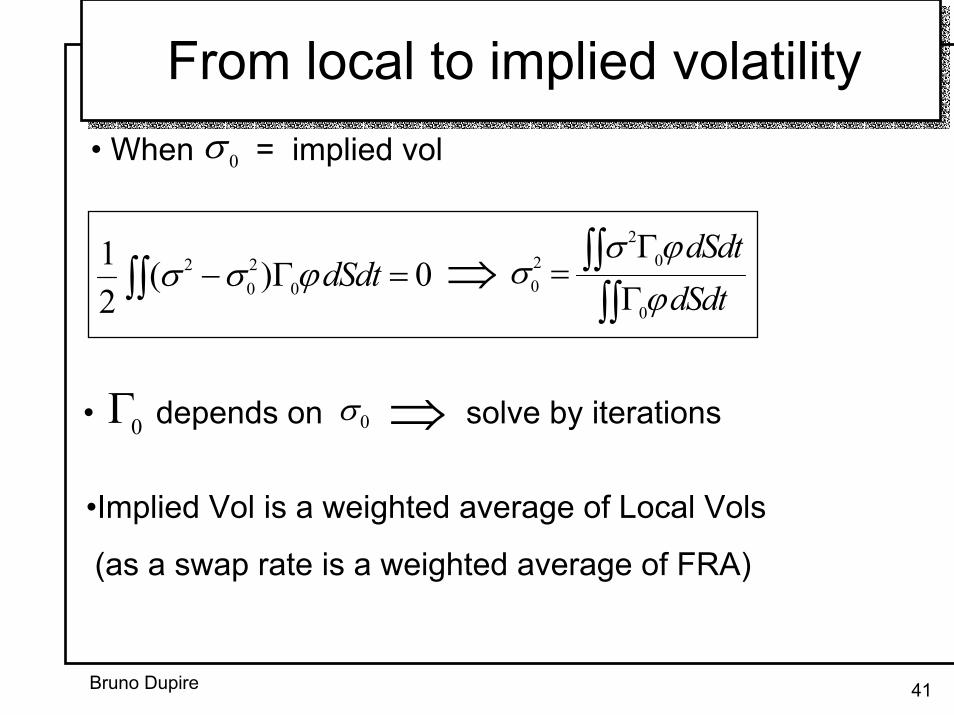
Bruno Dupire 41
From local to implied volatility• When = implied volσ 0
12
0202
0( )σ σ ϕ− =∫∫ Γ dSdt σσ ϕ
ϕ02
20
0
= ∫∫∫∫
Γ
Γ
dSdtdSdt⇒
⇒• depends onΓ0 0σ solve by iterations
•Implied Vol is a weighted average of Local Vols
(as a swap rate is a weighted average of FRA)

Bruno Dupire 42
Weighting scheme•Weighting Scheme: proportional to Γ0 ϕ
Out of themoneycase:
tS
Γ0 ϕ
At themoneycase:
S0=100K=100
S0=100K=110

Bruno Dupire 43
Weighting scheme (2)• Weighting scheme is roughly proportional to the brownian bridge density
Brownian bridge density:
( ) [ ]BB x t P S x S KK T t Tϕ , , = = =

Bruno Dupire 44
Time homogeneous case
S0
S
Kα(S)
TM (K>S0)
( )αϕ
ϕS
dt
dSdt=
∫∫∫
Γ
Γ
0
0
$ ( ) ( )σ α σ2 2= ∫ S S dS
ATM (K=S0) OS0
S
α(S)
σ Tsmall
S0
S
α(S) S0
S
Kα(S)
largeσ T

Bruno Dupire 45
Link with smile
S0
K2
K1
t
and are
averages of the same local
vols with different weighting
schemes
$σ K1$σ K2
=> New approach gives us a direct expression for the smile from the knowledge of local volatilities
But can we say something about its dynamics?

Bruno Dupire 46
Smile dynamics
23.5
24
24.5
25
25.5
26
S0 K
t
S1
Weighting scheme imposes some dynamics of the smile for a move of the spot:For a given strike K,
(we average lower volatilities)S K↑ ⇒ ↓$σ
Smile today (Spot St)
StSt+dt
Smile tomorrow (Spot St+dt)in sticky strike model
Smile tomorrow (Spot St+dt)if σATM=constant
Smile tomorrow (Spot St+dt)in the smile model
&

Bruno Dupire 47
Sticky strike model
A sticky strike model ( ) is arbitrageable.( )$ $σ σK Kt =
Let us consider two strikes K1 < K2
The model assumes constant vols σ1 > σ2 for example
σ1 dt
σ2 dt
1C(K1 )
Γ 1/Γ 2*
C(K 2)
σ1 dt
dt2σ
1C(K1 )
1C(K
2)
By combining K1 and K2 options, we build a position with no gamma andpositive theta (sell 1 K1 call, buy Γ1/Γ2 K2 calls)

Bruno Dupire 48
Vega analysis
•If & are constantσ σ0
C C dSdt( ) ( ) ( )Σ Σ Γ= + − ∫∫02
02
0
12
σ σ ϕ
σ σ ε202= +•
∫∫Γ+=+ dSdtCC ϕεσεσ 020
20 2
1)()({
2
2
∂σ∂ C
∂∂σ
∂∂σ
∂σ∂σ
∂∂σ
σC C C
= ⋅ = ⋅2
2
2 2Vega =

Bruno Dupire 49
Gamma hedging vs Vega hedging
• Hedge in Γ insensitive to realisedhistorical vol
• If Γ=0 everywhere, no sensitivity to historical vol => no need to Vega hedge
• Problem: impossible to cancel Γ now for the future
• Need to roll option hedge• How to lock this future cost?• Answer: by vega hedging
Bruno Dupire 50
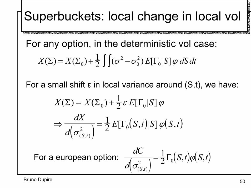
Superbuckets: local change in local vol
X X E S dS dt( ) ( ) ( ) [ | ]Σ Σ Γ= + −∫∫02
02
012 σ σ ϕ
For any option, in the deterministic vol case:
For a small shift ε in local variance around (S,t), we have:
( ) ( ) ( )
X X E S
dXd
E S t S S tS t
( ) ( ) [ | ]
[ , | ] ,( , )
Σ Σ Γ
Γ
= +
⇒ =
0 0
2 0
12
12
ε ϕ
σϕ
( ) ( ) ( )dCd
S t S tS tσ
ϕ( , )
, ,2 0
12= ΓFor a european option:

Bruno Dupire 51
Superbuckets: local change in implied vol
Local change of implied volatility is obtained by combininglocal changes in local volatility according a certain weighting
( ) ( )( )( )
dCd
dCd
dd$ $σ σ
σσ2 2
2
2= ∫
weighting obtainusing stripping
formula
sensitivity in local vol
Thus: cancel sensitivity to any move of implied vol
<=> cancel sensitivity to any move of local vol<=> cancel all future gamma in expectation

Bruno Dupire 52
Conclusion
• This analysis shows that option prices are based on how they capture local volatility
• It reveals the link between local vol andimplied vol
• It sheds some light on the equivalencebetween full Vega hedge (superbuckets) and average future gamma hedge
Bruno Dupire 53
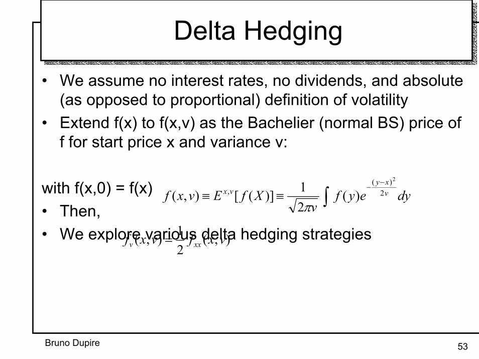
Delta Hedging
• We assume no interest rates, no dividends, and absolute (as opposed to proportional) definition of volatility
• Extend f(x) to f(x,v) as the Bachelier (normal BS) price of f for start price x and variance v:
with f(x,0) = f(x)• Then,• We explore various delta hedging strategies),(1),( vxfvxf =
∫−
−≡≡ dyeyf
vXfEvxf v
xyvx 2
)(,
2
)(21)]([),(π
2 xxv

Bruno Dupire 54
Calendar Time Delta Hedging
• Delta hedging with constant vol: P&L depends on the path of the volatility and on the path of the spot price.
• Calendar time delta hedge: replication cost of
• In particular, for sigma = 0, replication cost of ∫ −+t
uxx dudQVfTXf0
2,0
20 )(
21).,( σσ
)).(,( 2 tTXf t −σ
∫+t
uxxdQVfXf0 ,00 2
1)(
)( tXf

Bruno Dupire 55
Business Time Delta Hedging
• Delta hedging according to the quadratic variation: P&L that depends only on quadratic variation and spot price
• Hence, for
And the replicating cost of isfinances exactly the replication of f until
txtxxtvtxtt dXfdQVfdQVfdXfQVLXdf =+−=− ,0,0,0 21),(
,,0 LQV T ≤
t
t
uuxtt dXQVLXfLXfQVLXf ∫ −+=−0 ,00,0 ),(),(),(
),( ,0 tt QVLXf − ),( 0 LXf
),( 0 LXf LQV =ττ ,0:

Bruno Dupire 56
Daily P&L Variation

Bruno Dupire 57
Tracking Error Comparison

V. Stochastic Volatility Models
Bruno Dupire 59
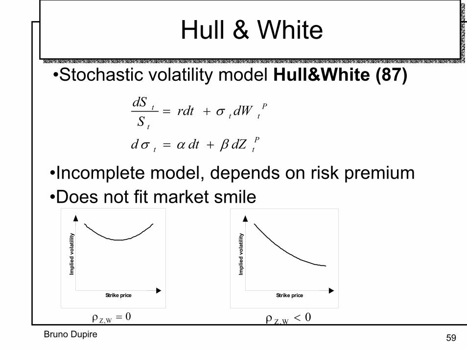
Hull & White•Stochastic volatility model Hull&White (87)
Ptt
Ptt
t
t
dZdtd
dWrdtS
dS
βασ
σ
+=
+=
•Incomplete model, depends on risk premium•Does not fit market smile
Strike price
Impl
ied
vola
tility
Strike price
Impl
ied
vola
tility
ρ Z W, < 0ρZ W, = 0

Bruno Dupire 60
Role of parameters
• Correlation gives the short term skew• Mean reversion level determines the long term
value of volatility• Mean reversion strength
– Determine the term structure of volatility– Dampens the skew for longer maturities
• Volvol gives convexity to implied vol• Functional dependency on S has a similar effect
to correlation

Bruno Dupire 61
Heston Model
( )
=+−=
+=
dtdZdWdZvdtvvdv
dWvdtS
dS
ρηλ
µ
,
Solved by Fourier transform:
( ) ( ) ( )τττ
τ
,,,,,,
ln
01, vxPvxPevxC
tTK
FWDx
xTK −=
−=≡

Bruno Dupire 62
Spot dependency
2 ways to generate skew in a stochastic vol model
-Mostly equivalent: similar (St,σt ) patterns, similar future evolutions-1) more flexible (and arbitrary!) than 2)-For short horizons: stoch vol model local vol model + independent noise on vol.
( ) ( )( ) 0,)2
0,,,)1≠
==ZW
ZWtSfxtt
ρρσ
0S
ST
σ
ST
σ
0S

Bruno Dupire 63
Convexity Bias
[ ]( )
===⇒=
=
0,?| 2
022
ZWKSEdZd
dWdS
ttt
t
ρσσασ
σ
[ ] 20
2only NO! σσ =tE
tσ likely to be high if 00 or SSSS tt <<>>
[ ]KSE tt =| 2σ
0S
20σ
K

Bruno Dupire 64
Impact on Models
• Risk Neutral drift for instantaneous forward variance
• Markov Model:fits initial smile with local vols( ) dWtSf
SdS
tσ,= ( )tS ,σ
( ) ( )]|[
,, 2
2
SSEtStSf
tt ==⇔
σσ

Bruno Dupire 65
Smile dynamics: Stoch Vol Model (1)
Skew case (r<0)
- ATM short term implied still follows the local vols
- Similar skews as local vol model for short horizons- Common mistake when computing the smile for anotherspot: just change S0 forgetting the conditioning on σ :if S : S0 → S+ where is the new σ ?
Local vols
+S0S−S
−S Smile
0 Smile S+S Smile
K
σ
[ ] ( )( )TKKSE TT ,22 σσ ==

Bruno Dupire 66
Smile dynamics: Stoch Vol Model (2)
• Pure smile case (r=0)
• ATM short term implied follows the local vols• Future skews quite flat, different from local vol
model• Again, do not forget conditioning of vol by S
Local vols−S Smile
0 Smile S
+S Smile
−S 0S +S K
σ

Forward Skew

Bruno Dupire 68
Forward Skews
In the absence of jump :
model fits market
This constrains
a) the sensitivity of the ATM short term volatility wrt S;
b) the average level of the volatility conditioned to ST=K.
a) tells that the sensitivity and the hedge ratio of vanillas depend on the calibration to the vanilla, not on local volatility/ stochastic volatility.
To change them, jumps are needed.
But b) does not say anything on the conditional forward skews.
),(][, 22 TKKSETK locTT σσ ==∀⇔

Bruno Dupire 69
Sensitivity of ATM volatility / S
S∂∂ 2σ
At t, short term ATM implied volatility ~ σt.
As σt is random, the sensitivity is defined only in average:
dSS
tStSttSSSSSE loctloctloctttttt ⋅
∂∂
≈−−++=+=−+),()(),(][
22222 σσδδσδσσ δδ
2ATMσIn average, follows .2
locσOptimal hedge of vanilla under calibrated stochastic volatility corresponds to perfect hedge ratio under LVM.