Bruno Deffains, Romain Political Self-Serving Bias ... · Political Self-Serving Bias and...

Discussion Paper No. 2015-

Bruno Deffains, RomainEspinosa, Christian Thoeni

December 2015

Political Self-Serving Biasand Redistribution

CeDEx Discussion Paper SeriesISSN 1749 - 3293

22

The Centre for Decision Research and Experimental Economics was founded in2000, and is based in the School of Economics at the University of Nottingham.

The focus for the Centre is research into individual and strategic decision-makingusing a combination of theoretical and experimental methods. On the theory side,members of the Centre investigate individual choice under uncertainty,cooperative and non-cooperative game theory, as well as theories of psychology,bounded rationality and evolutionary game theory. Members of the Centre haveapplied experimental methods in the fields of public economics, individual choiceunder risk and uncertainty, strategic interaction, and the performance of auctions,markets and other economic institutions. Much of the Centre's research involvescollaborative projects with researchers from other departments in the UK andoverseas.

Please visit http://www.nottingham.ac.uk/cedex for more information aboutthe Centre or contact

Suzanne RobeyCentre for Decision Research and Experimental EconomicsSchool of EconomicsUniversity of NottinghamUniversity ParkNottinghamNG7 2RDTel: +44 (0)115 95 14763Fax: +44 (0) 115 95 [email protected]

The full list of CeDEx Discussion Papers is available at

http://www.nottingham.ac.uk/cedex/publications/discussion-papers/index.aspx

Political Self-Serving Bias and Redistribution

Bruno Deffains, Romain Espinosa, Christian Thoni

November 12, 2015

Abstract

We explore the impact of the self-serving bias on the supply and demand for re-distribution. We present results from an experiment in which participants decide onredistribution after performing a real effort task. Dependent on individual performance,participants are divided into two groups, successful and unsuccessful. Participants’ suc-cess is exogenously determined, because they are randomly assigned to either a hardor easy task. However, because participants are not told which task they were assignedto, there is ambiguity as to whether success or failure should be attributed to internalor external factors. Participants take two redistribution decisions. First, they choose asupply of redistribution in a situation where no personal interests are at stake. Second,they choose a redistributive system behind a veil of ignorance. Our results confirm andexpand previous findings on the self-serving bias: successful participants are more likelyto attribute their success to their effort rather than luck, and they opt for less redis-tribution. Unsuccessful participants tend to attribute their failure to external factorsand opt for more redistribution. We demonstrate that the self-serving bias contributesto a polarization of the views on redistribution.

JEL codes: K10, H3.

Keywords: Redistribution, self-serving bias, experimental, veil of ignorance, polarization

Acknowledgments We thank the editor, Tim Cason, and two anonymous referees for their very

constructive remarks. We are also grateful to the participants of the annual congresses of the European

Association of Law and Economics (2014, Aix-en-Provence, France), the Louis Andre Gerard Varet (2015,

Aix-en-Provence, France) and the Association Francaise de Sciences Economiques (2015, Rennes, France).

We are also indebted to Stefan Voigt, Jerg Gutmann and the members of the Institute for Law and Economics

of Hamburg for their helpful comments.

1 Introduction

Political polarization has been recognized as a challenge for finding political consensus onsocial and economic issues. Keefer & Knack (2002) argue that polarization increases legaluncertainty and thereby hinders growth. Alt & Lassen (2006) provide evidence for higher

1

2

variations in political business cycles in politically more polarized countries. Other studieshave concluded that polarization reduces the likelihood to obtain broad consensus for policychanges and increase collective decision-making costs (Alesina & Drazen (1991), Rodrik(1999)). What makes societies polarized? Sunstein (2011) emphasizes the role of groups inunifying their members’ views with respect to a shared political agenda, which results instronger polarization across groups. In this article we provide evidence that the experienceof success and failure contributes to the polarization in political views.

Our work focuses at a particular domain of social consensus, namely the degree of redis-tribution between rich and poor members of the society. The recent resurgence of inequalitiesin democratic countries has led to a renewed interest in the questions of redistribution.1 Agreat body of research has sought to understand the factors driving the demand and the sup-ply of redistribution.2 Both empirical (Alesina & Angeletos 2005) and experimental works(Frohlich et al. 1987) have documented the heterogeneity of preferences regarding redistri-bution. Our research goes one step further, showing that views on redistributive systemsare not only shaped by individual preferences, but also malleable by economic experience.In an experimental setting we demonstrate that having been successful in a real effort taskmakes participants less likely to redistribute income between two other participants, andless likely to opt for redistributive systems behind a veil of ignorance. Unlike studies usingeliciting views about redistribution in field settings we can randomly assign participants tothe success and failure condition.

Our analysis builds on previous works on the self-serving bias (SSB hereafter). Theoriesabout the SSB postulate that individuals show a tendency to attribute their failure to situ-ational factors, and their success to their own dispositions.3 In other words, the SSB claimsthat, when an individual succeeds at a task, she tends to congratulate herself for her efforts,while she is more prompt to blame the situation when she fails. The SSB predicts thereforea tight relationship between wealth and the perception of the causes of poverty: wealthierindividuals are more likely to believe that they deserve their wealth. Considering the abovediscussion, this might have two effects on the political market. First, the self-serving biasmay affect voters whenever they believe that they are successful in life: because people arenot willing to recognize that their success is due to random events, they are more likely tosupport low tax rates. Second, the SSB might also be at play on the supply side of the po-litical market: when deciding on redistribution, politicians are also influenced by their ownexperience, and, thus, exposed to the SSB. In this work, we investigate both dimensions ofredistribution. On the one hand, we explore how participants are affected by the SSB whenthey decide redistribution for other individuals, having no personal interests at stake (supplyside). On the other hand, we analyze how participants’ preferences toward redistribution are

1Various recent works have documented this phenomenon (World: Atkinson (2003), Piketty & Saez(2006); US: Piketty & Saez (2003); Germany: Dustmann et al. (2009)).

2The literature has investigated egoistic concerns Corneo & Gruner (2002), Milanovic (2000), altruisticmotivations Fong (2001), Boarini & Le Clainche (2009), social considerations and future perspectives Keely& Tan (2008).

3Miller & Ross (1975) describe the SSB as “[. . . ] people indulge both in self-protective attributions underconditions of failure and in self-enhancing attributions under conditions of success”. See also Mezulis et al.(2004) for a recent meta study. For applications in the economic literature see e.g. Babcock et al. (1995), orBabcock & Loewenstein (1997).

3

modified by the SSB when they must decide for a redistribution rule that will affect theirunknown future own payoffs (demand side).

In accordance with the literature on the SSB we find that succeeding or failing in a taskgives rise to systematically different attributions and subsequent redistribution decisions.These findings suggest that increased inequality might have a particularly strong impact onpolarizing views about redistribution. Rich people do not only oppose redistribution becausethey expect to be net payers, but also because the SSB systematically shifts their fairnessprinciples. Likewise, poor people favor redistributive taxation not only because they expectfinancial gains, but also because the SSB leads them to shift the blame for their situation toexternal factors. Taken together this makes it difficult to reach a consensus and is likely toincrease political tensions across different strata of the society.

The rest of the paper is organized as follows. In Section 2 we discuss previous experimentson redistribution and the veil of ignorance. Section 3 describes the experiment and thepredictions. In Section 4 we present the results, and Section 5 concludes.

2 Literature Review

An early contribution to the experimental literature on redistribution is Frohlich et al. (1987),who investigate the choice of redistributive systems behind a veil of ignorance4, focusing onthe democratic process, where participants discuss the options until they reach an unanimousdecision. They find support for a redistribution scheme that maximizes the average incomewith a floor constraint. Later work focuses on individual choices for redistributive systemsand documents heterogeneity in redistributive preferences. Some studies argue that redis-tribution is mainly determined by self-interest (Hoffman & Spitzer (1985), Durante et al.(2014)), while other stress the role of social preferences (Tyran & Sausgruber (2006),Ackertet al. (2007), Schildberg-Hoerisch (2010), Balafoutas et al. (2013)). Klor & Shayo (2010)study the effect of group identity on redistribution and show that subjects tend to opt forredistribution which favors their group. Eisenkopf et al. (2013) analyze redistribution in asetting of unequal opportunities and find preferences for redistribution to be similar as ina setting where only risk affects the outcome. Gerber et al. (2013) conduct an experimentwhere they vary the ‘thickness’ of the veil of ignorance. Participants either (i) know noth-ing, (ii) have a noisy signal about their productivity, or (iii) have full information abouttheir productivity. They show that the level of redistribution is decreasing in the level ofinformation.

While these studies typically measure preferences for redistribution before the realizationof income, Frohlich & Oppenheimer (1990), Cabrales et al. (2012), Cappelen et al. (2007), andGroßer & Reuben (2013) investigate preferences for redistribution contingent on economicexperience. Close to our work is Kataria & Montinari (2012), who report results from anunequal opportunity treatment, where participants earn a payoff which partly depends on

4The experimental literature has made an extensive use of the veil of ignorance to analyze the preferencesfor redistribution net of selfish interests. The political economy literature has distinguished between twoversions of the veil of ignorance. According to Rawls, individuals should ignore everything they now abouttheir position, whereas Buchanan’s version of the veil requires only uncertainty about future outcomes (seee.g. Voigt (2015) for an overview.)

4

luck and partly on effort. After the realization of profit participants votes on tax rates. Inour design we combine the two approaches: we start with the realization of economic profitsand measure the effect of redistribution choices affecting only the allocation of the profits offuture economic activities. Furthermore, as opposed to the previous literature we choose adesign in which there is a high degree of ambiguity as to the causes of success or failure.

All the papers discussed so far focus on the choices of subjects who are directly affectedby the redistributive transfers. In contrast, Konow (2000) studies the behavior of subjectswho are not directly affected by the redistribution. He shows that these ‘disinterested dic-tators’ act according to the accountability principle, i.e. they are more likely to rewardindividuals based on their efforts, and to compensate them for back luck. Our design al-lows to investigate redistributive preferences in situations where the subject is not directlyinvolved (supply of redistribution), and when the subject is directly affected (demand forredistribution). The distinctive feature which distinguishes our experimental design fromthe previous literature is that instead of measuring preferences for redistribution we exoge-nously manipulate the participants’ experience of success or failure and measure the effecton redistributive preferences.

3 The Experiment

Our experiment explores the potential consequences of the self-serving bias on redistribution.Our protocol aims at generating a self-serving bias among participants, and capturing theeffects of this bias on both the supply of and the demand for redistribution.

3.1 Design

The experiment started with subjects earning money in a real effort task. The purpose ofthis task was to allocate the status of either ‘overachiever’ (to the subjects with an abovemedian performance among the subjects in a session), or ‘underachiever’ (to the remainingsubjects). This stage was followed by a manipulation check. After that we elicited ourtwo main measures of interest. First, subjects played the Disinterested Dictator Game(DGG), providing us with a measure of supply of redistribution. Second, we conductedthe Redistribution System Game (RSG) as a measure for the demand for redistribution.All interaction was anonymous and computerized. We used z-tree (Fischbacher 2007) toprogram the interface, and ORSEE (Greiner 2015) for recruitment.5

Real Effort Task. The real effort task consisted of a simple task of counting the onesin lines of binary digits. The screen contained 20 to 25 lines, with four to thirteen digitseach. Subjects had to indicate the number of ones occurring in each line. There were fiveconsecutive screens and there was a time limit of 25 seconds per screen. Correct answerswere rewarded by a certain number of tokens, depending on the condition they were assignedto. Half of the subjects were randomly assigned to the hard condition, the other half to theeasy condition. The maximum number of tokens was identical in both conditions. However,

5See online appendix E for the instructions and screen shots.

5

the tasks were designed such that it was very unlikely that a subject in the hard conditionwould earn more tokens than a subject in the easy condition. After completion of the fivescreens we used the number of tokens earned in the real effort task to perform a median splitof the subjects within a session. Subjects who earned more tokens than the median weretold that they performed above median (in the article we label them as overachievers), theother subjects were told that they performed below median (underachievers). The fact thatthe difficulty of the two tasks was sufficiently different ensured that the allocation of the taskdetermined whether a participant was an over- or underachiever. Any differences betweenover- and underachievers in the DDG or the RSG must then be caused by the allocation ofthe task, and not by self selection of subjects into treatment.6

Subjects were aware of the procedures. In the instructions we informed them that theycould be assigned either to an easy or to a hard task with equal probability. Participantswere also told that the maximum possible earnings were the same in both tasks. However,at no point in the experiment participants were told which task they were assigned to.While the two tasks clearly differed in difficulty, even the easy task was designed such thatnone of the participants managed to solve it perfectly, given the time limit. In addition,participants could not observe other participants’ tasks. Consequently, participants wereunable to deduce which task they were actually assigned to.

After the completion of the real effort task, participants were informed whether their per-formance was above or below the median. This information was followed by a manipulationcheck. Subjects answered six questions as to which extent they believed that their relativeachievement (success or failure) was due the following factors: (i) the task’s difficulty (Diff ),(ii) the introduction of the exercise (Intr), (iii) the clearness of the exercise (Clear), (iv)their effort (Eff ), (v) their will (Will), and (vi) their attention and focus (Focus). The firstthree questions identify situational factor, the last three questions individual factors.

Disinterested Dictator Game. For the DDG two participants (the ‘targets’) were ran-domly selected among all participants of the session.7 The remaining participants (the ‘dis-interested dictators’) were informed about the difference between the two targets’ incomesof the real effort task. The disinterested dictators had then the possibility to redistributetokens from the wealthier to the poorer target. All participants were told that the decisionof one disinterested dictator would be randomly selected and implemented. Participantswere also explicitly told that redistribution would concern only the two targets, and thatall others would not be affected by any redistribution mechanism in this task.8 Prior tothe decision, disinterested dictators were reminded that targets may have faced differenttasks. After every disinterested dictator made her choice, one redistribution proposal was

6In the two first sessions (standard sessions hereafter) four subjects in hard condition managed tobecome overachievers. Results from these sessions might be influenced by selection. In the results sectionwe will show that our results remain the same if we exclude these two sessions. For the remaining sessionswe increased the difference in the difficulty between hard and easy, and we observed a perfect separation.We will refer to the latter as gap-sessions. For a comparison of the two versions see online appendix C.

7In order to ensure comparability among our sessions, the selection process was set as follows. First, werandomly selected the first target. Second, we computed the difference of tokens between the first targetand the remaining participants. We then selected a participant such as to have a difference of tokens equalto twenty (or, if there was no exact match, as close to twenty as possible).

8Figure E1 in the appendix shows a screen shot of this stage.

6

randomly selected, and implemented. Disinterested dictators received their payoff from thereal effort task, while targets received their real effort task payoff corrected for redistribution.Finally the participants were informed about their final payoff. Importantly, the informationparticipants receive did not allow to infer any redistribution decision of other dictators.

We refer to this game as the Disinterested Dictator Game, because the dictator has thepower to redistribute, but–different from the dictator game–does not have his own profitat stake. The game is also different from the so-called third party dictator game (Fehr &Fischbacher (2004)), in which the classic dictator game is enriched by a third party who canpunish the dictator. A game similar to ours is presented by Konow (2000), who studies theaccountability principle. Konow investigates the redistribution choice of a dictator who is ei-ther exterior to the real effort task and has no stake in the redistribution, or who participatesto the game and has direct stakes in the redistribution. Konow refers to the two treatmentsas the Benevolent Dictator Treatment and the Standard Dictator Treatment. In our case,dictators have taken part in the real effort task but have no stake in redistribution. Previousworks in the literature, such as Durante et al. (2014), also used disinterested decision-makersto investigate redistribution decisions net of selfish interests.

Redistribution System Game. For the RSG participants were given new instructions.In these instructions, participants were told that they were going to be matched into groupsof four, and that they were going to perform another series of real effort tasks that weresubstantially different from what they did in the beginning of the experiment. Participantswere also informed that they were going to earn tokens in these real effort tasks, but thattheir payoffs would also be affected by random shocks, which could be either payoff increasingor payoff decreasing. Finally, the instructions said that, after each task and after each shock,redistribution was going to occur within each group according to the group’s redistributionsystem.

Participants were also informed that, prior to the real effort game, they would vote onredistribution systems. We presented three canonical redistribution systems to the par-ticipants. The libertarian system leaves each participant with her after-shock payoff (noredistribution). The egalitarian system sums up all individual after-shock payoffs within thegroup, and redistributes the sum in equal shares to the group members (full redistribution).Finally, the social-liberal system sums up all individual after-shock payoffs within the group,and redistributes the sum proportionally to the individual pre-shock payoffs (effort-basedredistribution). Subjects could indicate their preferences for the three systems in the vote,i.e., apart from the ‘pure’ systems, they could also implement a mixture of the systems. Toaid understanding the instructions contained a table showing how each redistribution systemaffects their final payoffs for given pre-shock and after-shock payoffs. Before turning to thevote, we presented the participants with control questions to ensure that the three redistri-bution principles were well understood. In four of the six sessions the control questions werethree general statements about the redistribution systems and participants had to indicatewhether they were correct or not (baseline sessions, for the instructions see Appendix E.2).In these sessions there are two sources of ambiguity: participants do not know the task theywill have to perform and they receive no specific information about the random shock. Inthe two remaining sessions we eliminated the ambiguity about the random shock and in-

7

formed the participants that the shock would change their income by −5,−4, . . . , 4, 5 tokenswith equal probability (extended sessions, instructions in Appendix E.3). Furthermorewe implemented different control questions, in which participants were asked to computehypothetical after-redistribution payoffs for a given set of pre-redistribution payoffs of thefour group members. The examples comprised four redistribution systems: 100% libertar-ian, 100% egalitarian, 100% social-liberal, and 50% libertarian 50% social-liberal (AppendixFigure E2).9

After the presentation of the redistribution systems, participants were asked to assignweights wi between 0 and 10 to each of the three redistribution systems. Participants weretold that one group member’s set of choices would be randomly chosen and implementedfor the group. Given three weights w1, w2 and w3 we computed a triplet of relative weightsvi = wi

w1+w2+w3, i = 1, 2, 3. For each of the real effort tasks a participant’s final payoff is equal

to v1% (resp. v2% and v3%) of the payoff that she would have earned under the canonicalsystem 1 (resp. 2 and 3).

After the vote and the determination of the redistribution system participants were in-formed about the redistribution system selected for their group. A screen displayed thecomposition in terms of percentages of the three canonical system. After that, participantsproceeded with the real effort tasks. They had to read a short text (approx 140 words) andcount the number of misspelled words. The individual (pre-shock and pre-redistribution)profit of the task was equal to the 20 tokens minus four times the absolute difference be-tween the reported number of mistakes and the real number of mistakes in the text. Aftereach real effort task participants learned their initial profit, their profit after the shock,and their final profit (including redistribution). Then participants were asked (1) whetherthey were satisfied with the implemented redistribution system, and (2) whether they feltreinforced in their original choice. The experiment ended after four real effort tasks.

The RSG is inspired by the experiment reported in Frohlich & Oppenheimer (1990),where subjects choose a redistribution system without knowing the nature of the task theyare about to perform. Once a redistribution system has been selected, subjects are givena series of texts to correct (spelling mistakes). The choice of redistribution systems followsGerber et al. (2013).

3.2 Hypotheses

Our experimental protocol aimed at investigating how the self-serving bias may impact thesupply and the demand of redistribution. We create a situation in which participants areaware of their relative status in the population, but have limited information about whetherthey should attribute the outcome to luck or effort. The real effort task in the beginningof the experiment creates two kinds of participants: those who performed better than themedian participant (overachievers), and those who performed worse than the median par-ticipant (underachievers). We hypothesize that this manipulation induces a self-serving biasamong participants: overachievers tend to attribute the outcome to their efforts, whereasunderachievers tend to attribute the outcome to bad luck. The Disinterested Dictator Game

9Using control questions presumably enhances subjects’ understanding of the mechanisms, but it mighthave the disadvantage that the experimenter has to pick specific actions of the game as examples, whichmight influence subsequent behavior, see Roux & Thoni (2015).

8

measures the impact of this change of the perceptions of causality on the supply of redistribu-tion towards third parties. Indeed, as Konow (2000) showed, people decide on redistributionaccording to the accountability principle, i.e. they reward people proportionally to theirlevel of effort. By affecting the perception of the role played by effort in the final outcome,we expect the self-serving bias to affect the supply of redistribution: overachievers (under-achievers) will be more likely to believe that efforts (random factors) determine success, andwill therefore be less (more) likely to redistribute. Because decision-makers profits are notaffected by redistribution, our protocol allows us to isolate how the redistribution is changedby the perception of the causes of success in the absence of selfish interests.10 Our predictionwith regard to the DDG is:

Prediction 1 Overachievers will redistribute less than underachievers.

In the Redistribution System Game participants are asked to express their preferencesover three redistribution systems. Unlike in the first game, participants’ redistribution deci-sions at the beginning of the second game are designed to affect their own future (unknown)payoff. The ex-ante choice about the redistribution systems ensures that participants expresstheir demand for redistribution behind a veil of ignorance, i.e., not knowing the nature of thereal effort task.11 Following the same argument as for prediction 1, if the self-serving biaschanges one’s perception of the determinants of success, overachievers should be more likelyto believe that their future payoffs will be determined by their efforts than underachievers,and therefore express a lower demand for redistribution.

When taking a decision in the RSG game, participants presumably consider three factorsthat affect their future revenue: their level of effort, their ability in the (unknown) task,and the random shocks. The first factor is obviously endogenous, while the two latter areexogenous. The two exogenous factors result in uncertainty and risk. First, participantsface uncertainty regarding the nature of the task they are about to perform. Second, theyface risk concerning the shocks that they know to happen after each task. The libertariansystem corresponds to a situation without insurance. On the opposite, the egalitarian systeminsures against both risk and uncertainty: if an individual faces a task at which he/she isvery bad, he/she will receive transfers from other participants more capable at this task.Moreover, in the egalitarian system, shocks are fully compensated. However, the egalitariansystem comes at a cost, because it generates incentives to free ride. The social-liberal systemstands in-between: it redistributes according to the pre-shock payoff, which is determined bythe participants’ abilities and effort, but not by the shocks. Consequently, the social-liberalsystem provides an insurance against risk, but not against uncertainty.

Due to the self-serving bias a successful participant is more likely to see the outcomeas resulting from his/her own effort than a less successful participant. The self-serving biasis therefore likely to impact the demand for redistribution in cases where causation is notclearly determined. Thus, the self-serving bias should increase the demand for insurance

10Note that our experimental design minimizes the focus on the own profit at this stage. The onlyinformation participants receive when deciding in the DDG is the difference between the two targets’ payoffs.They have no information about absolute payoffs, not even their own payoff.

11Our protocol is close to Buchanan’s version of the veil of ignorance. (See footnote 4) We get rid ofimmediate egoistic interests by putting uncertainty on future outcomes.

9

against uncertainty for participants who performed relatively worse, because they expectthe nature of the task to play a predominant role in the determination of their payoff. Onthe other hand, random shocks are clearly exogenous. The self-serving should therefore nothave an impact on the demand for insurance against risk.

Three predictions follow from this discussion. First, we expect overachievers to have astronger preference for social-liberalism than underachievers. Conversely, we anticipate thatunderachievers will display a stronger demand for the egalitarian system.

Prediction 2A Overachievers will opt for less egalitarianism than underachievers.

Prediction 2B Overachievers will opt for more social-liberalism than underachievers.

In case of the libertarian system things are less clear. If the social-liberal system wasnot available, then this system would most likely be more preferable to overachievers thanunderachievers, for the reasons discussed above. However, when all three redistributionsystems are available, support for the libertarian system can only be explained if participantsprefer some of the risk to be uninsured, i.e., if they are to some extent risk seeking. We donot see an a priori reason why the status of under- or overachiever should systematicallyaffect risk preferences. Our prediction is therefore

Prediction 2C Overachievers and underachievers will not systematically differ in theirsupport for libertarianism.

4 Results

We ran six sessions with 24 participants each. All sessions were run in Strasbourg (Januaryand February 2014, July 2015). The sessions lasted about 45 minutes, and participantsearned on average 13.66 euro. We present our results in the order in which they wereelicited, starting with real effort task, followed by the Disinterested Dictator Game and theRedistribution System Game.

4.1 Real effort task

The experiment starts with a real effort task, in which subjects are asked to determinethe number of ones in binary sequences. This provides us with a measure for individualperformance. The left panel of Figure 1 shows the results of the real effort task. Subjectsrandomly allocated to the hard task scored on average 19.4 tokens (sd: 4.02), while subjectsin the easy task scored 33.6 (sd: 5.25) tokens. Spikes in the figure are standard errors,indicating that the difference between the hard and easy task is highly significant.

Based on the performance measure we classify our subjects into overachievers (abovemedian performance), and underachievers. In four sessions the hard/easy task was perfectlyseparating the population, i.e., all participants randomly allocated to the easy task turnedout to be overachievers, and vice versa. In the other sessions four participants with the hardtask managed to perform better than the median participant, and became overachiever.

10

Consequently, four participants with the easy task became underachiever. Note that ourprotocol induced the same level of information for both underachievers and overachieversregardless of their original task. It follows that participants were not able to deduce whetherthey were assigned to the hard or the easy task, such that presumably only the labelingas ‘above the median’ or ‘below the median’ affected their attributions. Consequently self-serving bias (SSB) can occur irrespective of the original task a participant was assignedto.

Before looking at the redistribution decisions, we perform a manipulation check to seewhether our protocol effectively induced a self-serving bias among participants. To do so,we compare answers to the six questions as to whether subjects attribute their success (orfailure) to effort or luck. Comparing the average scores of overachievers and underachieversshows that the former gave systematically higher scores to all questions (see Table 1 inthe appendix). To compare the relative weight of situational factors to the factors relatedto effort (individual), we define a measure Fatalism as the ratio between the sum of thescores for the three situational factors and the sum of the scores for the individual factors.The middle panel of Figure 1 shows the results. We find a clear and significant differencein Fatalism between the two groups: With a ratio of 1.30 underachievers put a higherrelative weight on situational factors than overachievers (0.94). The difference is significant atp = .003 (two-sample t-test).12 To conclude, the experience of being an under- or overachieversystematically affects the way participants attribute the outcome to internal and externalfactors. While overachievers tend to emphasize their own contribution, underachievers tendto focus on external factors, i.e., develop a more fatalist attitude. We see this as a clearindication for a self-serving bias. In a next step we investigate whether the differencesbetween over- and underachievers affect redistribution decisions.

4.2 DDG: Supply of Redistribution

Recall that in the disinterested dictator game redistribution affects only targets’ payoffs.Dictators were specifically told that no redistribution would affect their own payoff in thisgame. Since we have some variation in the differences between the two targets’ profitsacross sessions we calculate the percentage of the payoff difference to be redistributed formthe richer to the poorer target. Zero corresponds to leaving the incomes unchanged, whilereallocating 50 percent of the difference means that the two profits are equalized. Overallwe observe a redistribution of 37.4 percent; 17.4 percent of the subjects do not redistributeat all, while 41.7 percent of the subjects implement a solution which equalized payoffs.

Prediction 1 links a person’s status after the real effort task to the supply of redistri-bution. The right panel of Figure 1 shows the average redistribution percentage chosenby underachievers and overachievers (RedSupply). The difference is substantial and signifi-cant: Underachievers redistribute 43.9 percent while overachievers redistribute 30.9 percent(p = .003, two-sample t test).13 In the online appendix we provide additional analyses tocheck the robustness of our results on Fatalism and the redistribution decision. First, we

12The results are very similar if we consider only the gap sessions (1.21 vs. 0.90); and the differenceremains significant (p = .012).

13The effect size is almost identical if we consider only the gap sessions (42.2 percent vs. 29.9 percent);and the difference remains significant (p = .015).

11

010

20

30

40

Easy

Hard

Real effort taskT

oken

s

.5.7

51

1.2

51.5

Over-achiever

Under-achiever

Attribution

Fata

lism

0%

20%

40%

60%

Over-achiever

Under-achiever

DDG

Red

Supply

Figure 1: Left panel: Average number of tokens earned in the hard and easy real effort task.Middle panel: Levels of Fatalism, defined as the ratio between external and internal factors,for over- and underachievers. Right panel: Percentage redistributed in the disinteresteddictator game. Spikes show standard errors.

perform a permutation test (two-sided p = .001 and p = .001, see Figures B1 and B2 inthe online appendix); second we run OLS estimates controlling for individual characteris-tics gender, political orientation, age, and the practice of competitive sport, as well as adummy for the gap sessions (online appendix Table A1).14 The effect of overachiever ishighly significant in all specifications, while none of the other covariates seem to explain theredistribution decision. This leads to our first result:

Result 1 Overachievers redistribute less money from the rich to the poor target thanunderachievers.

4.3 RSG: Demand for redistribution

We now turn to the analysis of the preferences over the redistribution systems in the secondgame. Because participants were told that the real effort tasks of the second game would besubstantially different from the first real effort task, they were a priori not able to predicttheir productivity and their relative abilities and in the task. In this regard, the decisionsmade at the beginning of the second game are taken behind a veil of ignorance. As opposedto the DDG, redistribution now affects the own payoff, which means that decisions can beinterpreted as demand for redistribution.

The choice of a redistribution system is measured by the importance levels indicatedfor each of the three canonical systems. For the following analysis we normalize the scores

14Our results are also robust when we cluster standard errors on the session level. Because of the smallnumber of clusters, we implemented wild bootstrapping to obtain robust p-values such as suggest by Cameron& Miller (2015). See model 5 in Table A2 of the online appendix for the results.

12

0%

20%

40%

60%

Over-achiever

Under-achiever

Over-achiever

Under-achiever

Over-achiever

Under-achiever

Egalitarian Social-liberal Libertarian

Rel

ative

wei

ght

Figure 2: Results from the Redistribution System Game. Bars show average relative weightgiven to the respective redistribution system. Spikes show standard errors.

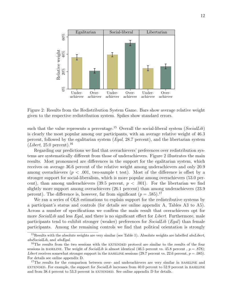
such that the value represents a percentage.15 Overall the social-liberal system (SocialLib)is clearly the most popular among our participants, with an average relative weight of 46.3percent, followed by the egalitarian system (Egal, 28.7 percent), and the libertarian system(Libert, 25.0 percent).16

Regarding our predictions we find that overachievers’ preferences over redistribution sys-tems are systematically different from those of underachievers. Figure 2 illustrates the mainresults. Most pronounced are differences in the support for the egalitarian system, whichreceives on average 36.6 percent of the relative weight among underachievers and only 20.9among overachievers (p < .001, two-sample t test). Most of the difference is offset by astronger support for social-liberalism, which is more popular among overachievers (53.0 per-cent), than among underachievers (39.5 percent, p < .001). For the libertarian we findslightly more support among overachievers (26.1 percent) than among underachievers (23.9percent). The difference is, however, far from significant (p = .585).17

We ran a series of OLS estimations to explain support for the redistributive systems bya participant’s status and controls (for details see online appendix A, Tables A3 to A5).Across a number of specifications we confirm the main result that overachievers opt formore SocialLib and less Egal, and there is no significant effect for Libert. Furthermore, maleparticipants tend to exhibit stronger (weaker) preferences for SocialLib (Egal) than femaleparticipants. Among the remaining controls we find that political orientation is strongly

15Results with the absolute weights are very similar (see Table 1). Absolute weights are labelled absLibert,absSocialLib, and absEgal.

16The results from the two sessions with the extended protocol are similar to the results of the foursessions in baseline. The weight of SocialLib is almost identical (46.5 percent vs. 45.8 percent , p = .878);Libert receives somewhat stronger support in the baseline sessions (29.7 percent vs. 22.6 percent, p = .085).For details see online appendix D.

17The results for the comparison between over- and underachievers are very similar in baseline andextended. For example, the support for SocialLib increases from 40.0 percent to 52.9 percent in baselineand from 38.4 percent to 53.3 percent in extended. See online appendix D for details.

13

related to the support for Libert and Egal. Participants who indicate that they are politicallycloser to the right opt for more Libert and less Egal.18 In the estimates with controls we findthat the sessions where we provided more information about the shock (extended) tendsto increase the support for Libert and decrease the support for Egal.

Taken together the evidence clearly supports our predictions 2A to 2C: The self-servingbias affects the demand of insurance against uncertainty, but not the demand of insuranceagainst risk. Underachievers are more likely to prefer full insurance than overachievers(egalitarianism), while overachievers display a stronger preference for a system that insuresonly against risk.

Result 2 Overachievers have a stronger preference for the social-liberal system than under-achievers, who, in turn, have a stronger preference for egalitarianism. We find no significantdifferences in the support for the libertarian system.

5 Conclusion

Our paper investigates the consequences of the self-serving bias on redistribution choices. Todo so, we run an experiment in which we induce a self-serving bias among participants. Toisolate the effects of the self-serving bias from selfish interests, we make participants chooseon the level of redistribution in a disinterested manner or behind a veil of ignorance. Thisallows us to assess the impact of the self-serving bias on both the supply and the demand ofredistribution.

We conclude on two far-reaching results. We show that participants with a good (resp.bad) relative success status display a lower (higher) supply of redistribution, because theyare on average more (less) likely to believe that their outcome result from their effortscompared to participants with a bad (good) relative success status. Second, we show thatthe self-serving bias also affects the demand of redistribution in the same manner, i.e., byreducing (resp. increasing) the demand for redistribution for relatively successful (resp. lesssuccessful) participants.

Our findings have significant implications for political debates on redistribution, as theself-serving bias polarizes both the supply and the demand of redistribution. The increasein polarization resulting from the self-serving bias rises numerous questions. First of all, itasks a normative question: Is the increased polarization of the political debate necessaryharmful for society? Previous works in the literature presented in the introduction tendto indicate that political polarization has negative effects on economic growth. One could,however, also postulate that the increased polarization might strengthen the competitionon the political market by forcing parties to propose different platforms. Even considering

18In the instructions and on the screen we used the same labels for the three systems as in this article.We cannot therefore rule out the possibility that the preferences for the libertarian system by the rightistparticipants are driven by a (to them) appealing label. However, given the random assignment of theeasy and hard task, political orientation should be identically distributed across groups (overachievers vs.underachievers). Indeed we observe no significant difference between the two groups (two-sample t-test:p = .595). It follows that the lack of significance of the overachiever status cannot be attributed to labellingissues.

14

that the heterogeneity of preferences is not necessary harmful for the system, it is howeverlegitimate to wonder whether the increase of polarization resulting from the self-serving biasis welfare enhancing. This increase of polarization seems indeed to result from partly con-tingent economic experience. In other words, the self-serving bias might generate volatilevariations in the political preferences toward redistribution. Although society might bene-fit from divergence of opinions, collective decision-making may suffer from such variations.Third, considering that the self-serving bias might create unnecessary polarization, a le-gitimate question is whether institutions should seek to unbias citizens. The literature onnudges argues that society might benefit from making use of psychological mechanisms aspolicy tools (Thaler & Sunstein 2008). Two questions follow. First, is it legitimate for thegovernment to unbias citizens regarding redistribution, given that the government has itsown –maybe also biased– view about redistribution? Second, what is the unbiased amountof redistribution one individual would have wanted if she did not experience her economiccondition?

Our experimental approach to induce a SSB with regard to success and failure could beexpanded to study a number of interesting questions. First, our protocol aimed at induc-ing a self-serving bias among participants by creating two groups of individuals: over- andunderachievers. The dichotomous nature of our treatment is an experimental simplification,which is not realistic. Expanding the design to a continuous setting would allow to investi-gate how the SSB and redistributive choices would react to fine-grained changes in relativeperformance. Second, it would be interesting to explore the potential of information to un-bias the participants and reduce the polarization. One of the least controversial means tounbias individuals might be to disseminate scientific evidence about the relative importanceof external and internal factors in the determination of the position in the social hierarchy,such as the degree of intergenerational mobility (Bowles & Gintis 2002, Chetty et al. 2014).

15

6 Appendix: Summary statistics

Variable Source All Participants Underachievers Overachievers p-valueDiff MC 3.903 3.597 4.208 0.052

(1.893) (1.998) (1.744)Intr MC 4.604 4.472 4.736 0.412

(1.922) (2.143) (1.678)Clear MC 3.639 2.125 5.153 0.000

(2.295) (1.695) (1.758)Eff MC 3.951 3.333 4.569 0.000

(1.682) (1.601) (1.537)Will MC 4.042 2.653 5.431 0.000

(2.099) (1.567) (1.582)Focus MC 4.993 3.917 6.069 0.000

(1.83) (1.782) (1.105)Fatalism MC 1.116 1.297 .936 0.003

(.74) (.942) (.387)

RedSupply DDG .374 .439 .309 0.003(.25) (.246) (.24)

absLibert RSG 4.035 3.861 4.208 0.559(3.545) (3.562) (3.544)

absSocialLib RSG 7.021 6.431 7.611 0.026(3.194) (3.223) (3.074)

absEgal RSG 4.556 5.681 3.431 0.000(3.747) (3.626) (3.544)

Libert RSG .25 .239 .261 0.584(.232) (.238) (.226)

SocialLib RSG .463 .395 .53 0.001(.248) (.201) (.272)

Egal RSG .287 .366 .209 0.000(.255) (.261) (.226)

Table 1: Summary Statistics: mean and standard deviation (in parentheses); p-values cor-respond to bilateral two-group mean-comparison tests. MC stands for Manipulation Check,DDG for Disinterested Dictator Game and RSG for Redistribution System Game.

16

References

Ackert, L. F., Martinez-Vazquez, J. & Rider, M. (2007), ‘Social preferences and tax policydesign: Some experimental evidence’, Economic Inquiry 45(3), 487–501.

Alesina, A. & Angeletos, G.-M. (2005), ‘Fairness and redistribution’, American EconomicReview 95(4), 960–980.

Alesina, A. & Drazen, A. (1991), ‘Why are Stabilizations Delayed?’, American EconomicReview 81, 1170–1188.

Alt, J. E. & Lassen, D. D. (2006), ‘Transparency, Political Polarization, and Political BudgetCycles in OECD Countries’, American Journal of Political Science 50(3), 530–550.

Atkinson, A. B. (2003), ‘Income Inequality in OECD Countries: Data and Explanations’,CESifo Economic Studies 49, 479–513.

Babcock, L. & Loewenstein, G. (1997), ‘Explaining bargaining impasse: The role of self-serving biases’, Journal of Economic Perspective 11(1), 109–126.

Babcock, L., Loewenstein, G., Issacharoff, S. & Camerer, C. (1995), ‘Biased judgments offairness in bargaining’, American Economic Review 85(5), 1337–1343.

Balafoutas, L., Kocher, M. G., Putterman, L. & Sutter, M. (2013), ‘Equality, equity andincentives: An experiment’, European Economic Review 60, 32–51.

Boarini, R. & Le Clainche, C. (2009), ‘Social preferences for public intervention: An empiricalinvestigation based on french data’, Journal of Socio-Economics 38, 115–128.

Bowles, S. & Gintis, H. (2002), ‘The inheritance of inequality’, Journal of Economic Per-spectives 16(3), 3–30.

Cabrales, A., Nagel, R. & Rodriguez-Mora, J. V. (2012), ‘It is Hobbes, not Rousseau: Anexperiment on voting and redistribution’, Experimental Economics 15, 278–308.

Cameron, A. C. & Miller, D. L. (2015), ‘A practitioner’s guide to cluster-robust inference’,Journal of Human Resources 50(2), 317–372.

Cappelen, A. W., Hole, A. D., Sørensen, E. Ø. & Tungodden, B. (2007), ‘The pluralism offairness ideals: An experimental approach’, American Economic Review 97(3), 818–827.

Chetty, R., Hendren, N., Kline, P. & Saez, E. (2014), ‘Where is the land of opportunity?The geography of intergenerational mobility in the United States’, Quarterly Journal ofEconomics 129(4), 1553–1623.

Corneo, G. & Gruner, H. P. (2002), ‘Individual preferences for political redistribution’, Jour-nal of Public Economics 83, 83–107.

17

Durante, R., Putterman, L. & van der Weele, J. (2014), ‘Preferences for redistributionand perception of fairness: An experimental study’, Journal of the European EconomicAssociation 12(4), 1059–1086.

Dustmann, C., Ludsteck, J. & Schonberg, U. (2009), ‘Revisiting the German wage structure’,Quarterly Journal of Economics 124(2), 843–881.

Eisenkopf, G., Fischbacher, U. & Follmi-Heusi, F. (2013), ‘Unequal opportunities and dis-tributive justice.’, Journal of Economic Behavior and Organization 93, 51–61.

Fehr, E. & Fischbacher, U. (2004), ‘Third-party punishment and social norms’, Evolutionand Human Behavior 25(2), 63–87.

Fischbacher, U. (2007), ‘z-tree: Zurich toolbox for ready-made economic experiments’, Ex-perimental Economics 10(2), 171–178.

Fong, C. (2001), ‘Social preferences, self-interest, and the demand for redistribution’, Journalof Public Economics 82, 225–46.

Frohlich, N. & Oppenheimer, J. A. (1990), ‘Choosing justice in experimental democracieswith production’, American Political Science Review 84, 461–477.

Frohlich, N., Oppenheimer, J. A. & Eavey, C. L. (1987), ‘Laboratory results on Rawls’distributive justice’, British Journal of Political Science 17, 1–21.

Gerber, A., Nicklisch, A. & Voigt, S. (2013), Strategic choices for redistribution and the veilof ignorance. Working Paper.

Greiner, B. (2015), ‘Subject pool recruitment procedures: Organizing experiments withORSEE’, Journal of the Economic Science Association 1(1), 114–125.

Großer, J. & Reuben, E. (2013), ‘Redistribution and market efficiency: An experimentalstudy’, Journal of Public Economics 101, 39–52.

Hoffman, E. & Spitzer, M. L. (1985), ‘Entitlements, rights, and fairness: An experimen-tal examination of subjects’ concepts of distributive justice’, Journal of Legal Studies14(2), 259–297.

Kataria, M. & Montinari, N. (2012), ‘Risk, entitlement and fairness bias: Explaining prefer-ences for redistribution in multi-person setting’, Working Paper .

Keefer, P. & Knack, S. (2002), ‘Polarization, politics and property rights: Links betweeninequality and growth’, Public choice 111(1-2), 127–154.

Keely, L. C. & Tan, C. M. (2008), ‘Understanding preferences for income redistribution’,Journal of Public Economics 92, 944–961.

Klor, E. F. & Shayo, M. (2010), ‘Social identity and preferences over redistribution’, Journalof Public Economics 94, 269–278.

18

Konow, J. (2000), ‘Fair shares: Accountability and cognitive dissonance in allocation deci-sions’, American Economic Review 90(4), 1072–1091.

Mezulis, A. H., Abramson, L. Y., Hyde, J. S. & Hankin, B. L. (2004), ‘Is there a uni-versal positivity bias in attributions? a meta-analytic review of individual, developmen-tal, and cultural differences in the self-serving attributional bias’, Psychological Bulletin130(5), 711–747.

Milanovic, B. (2000), ‘The median-voter hypothesis, income inequality, and income redistri-bution: An empirical test with the required data’, European Journal of Political Economy16, 367–410.

Miller, D. T. & Ross, M. (1975), ‘Self-serving biases in the attribution of causality: Fact orfiction?’, Psychological Bulletin 82(2), 213–225.

Piketty, T. & Saez, E. (2003), ‘Income inequality in the united states 1913-1998’, QuarterlyJournal of Economics 118, 1–39.

Piketty, T. & Saez, E. (2006), ‘The evolution of top incomes: A historical and internationalperspective’, American Economic Review 96(2), 200–205.

Rodrik, D. (1999), ‘Where did All the Growth Go? External Shocks, Social Conflict, andGrowth Collapses’, Journal of Economic Growth 4(4), 385–412.

Roux, C. & Thoni, C. (2015), ‘Do control questions influence behavior in experiments?’,Experimental Economics 18(2), 185–194.

Schildberg-Hoerisch, H. (2010), ‘Is the veil of ignorance only a concept about risk? Anexperiment’, Journal of Public Economics 94, 1062–1066.

Sunstein, C. R. (2011), Going to Extremes: How Like Minds Unite and Divide, OxfordUniversity Press.

Thaler, R. H. & Sunstein, C. R. (2008), Nudge. Improving Decisions About Health, Wealth,and Happiness, Yale University Press, New Haven & London.

Tyran, J.-R. & Sausgruber, R. (2006), ‘A little fairness may induce a lot of redistribution indemocracy’, European Economic Review 50(2), 469–485.

Voigt, S. (2015), Veilonomics: On the use and utility of veils in constitutional politicaleconomy, in L. M. Imbeau & S. Jacob, eds, ‘Behind a Veil of Ignorance?’, Vol. 32, SpringerInternational Publishing, pp. 9–33.

1

Online Appendix

Political Self-Serving Bias and Redistribution

Bruno Deffains, Romain Espinosa, Christian Thoni

A Additional Analyses

In this section, we present the estimation results of the econometric specifications discussedin the paper. We perform a multivariate analysis of the degree of Fatalism, the redistributiondecision in the first game, and the weights of the three redistribution systems in the secondgame. Our set of explanatory variables includes a gender dummy and the participant’s age.Since redistribution is obviously a very political issue, we control for political orientation(10-point, left-right scale). Finally, we include a measure for whether the subject regularlyparticipates at sports competitions.

We run OLS regressions for eight dependent variables: the degree of fatalism, the supplyof redistribution in the DDG, the normalized importance levels given to each redistributionsystem in the RSG and the associated absolute importance levels. Using the best selectionmethod, we present different specifications, which progressively include additional indepen-dent variables, based on their explanatory power. We impose that our specifications includethe overachiever status and two dummies for the gap sessions (i.e., session 3 to 6) and adummy for extended to control for differences between the two versions of the controlquestions. The best selection method then includes additional variables according to theirexplanatory power. We present the C, the AICC and the BIC statistics. Tables A1 andA2 display the results for the Fatalism and RedSupply variables respectively. Tables A3,A4 and A5 display estimates of the normalized importance scores (Libert, SocialLib, Egal).Tables A6, A7 and A8 show respectively the results for absLibertarian, absSocialLib andabsEgalitarian.

In the main article we take the stand that data analyzed in the paper are independent atthe subject level. When participants make the essential decisions (Fatalism, RedSupply, andthe scores in the RSG), they have had very limited information about other participants’behaviors. In particular, when answering the questions determining the Fatalism score, par-ticipants knew only their relative position in the group. When choosing on the redistributionin the DDG, they learned only the difference of payoffs between the two targets. Finally,when choosing among redistribution systems in the RSG, participants knew only the twoprevious pieces of information plus their own profit at the end of the first game. It is thusnot possible to infer other subjects’ decisions about redistribution from the information re-ceived.19 For the models 1-5 in the Tables A1 to A8 we assume that the observations areindependent.

For model 5 in all these Tables we also cluster the data to check whether our estima-tions are robust to the violation of independence. Since we ran six experimental sessions,

19Note that the two subjects in each session in the role of the target in the DDG might draw some inferenceabout the redistribution choice of their dictator. However, even for them it is very difficult, because theyonly learn their final income, and not the change in the income due to the redistribution. All our resultsfrom the RSG hold if we exclude the targets from the analysis.

2

the clustering of the standard errors can be made on six clusters only. Recent works inthe econometric literature have investigated the properties of estimates with low numbersof clusters, and show that standard corrections underestimate the true standard errors. Inorder to deal with this issue, we use wild cluster bootstrapping to compute a robust p-valuefor our parameter of interest (overachiever). We follow the guidelines given by Cameron andMiler (2015).20 In addition to the OLS results of model 5, we report three statistics derivedfrom the wild-clustering for each regression. On the one hand, we present the Rademacherand Webb p-values associated with the treatment’s effect. These statistics are calculated forthe regressions including all covariates. They must be interpreted similarly the p-values ofthe statistical test associated to the null hypothesis for the overachiever variable (two-sidedtest). In other words, we claim that the overachiever variable has a significant impact whenthese p-values are below 5%. On the other hand, we report the distributions of the Webb andRademacher t-statistics from which we derived the p-values (Figures A1 to A8). Note that,in our case, the wild cluster bootstrap technique yields similar results to the non-clusteredresults.

20Cameron, A. C. & Miller, D. L. (2015), ‘A Practitioner’s Guide to Cluster-Robust Inference’, Journal ofHuman Resources 50(2), 317–372.

3

Model 1 2 3 4 5overachiever -0.361*** -0.368*** -0.377*** -0.380*** -0.387***

(0.119) (0.120) (0.121) (0.122) (0.123)gap -0.195 -0.194 -0.204 -0.214 -0.222*

(0.127) (0.127) (0.128) (0.130) (0.131)male -0.0774 -0.0707 -0.107 -0.101

(0.122) (0.123) (0.131) (0.131)sport 0.0805 0.0817

(0.146) (0.146)polit orient -0.0220 -0.0195

(0.0274) (0.0279)age 0.0104 0.00854

(0.0170) (0.0174)constant 1.427*** 1.553*** 1.319*** 1.459*** 1.250**

(0.119) (0.233) (0.448) (0.464) (0.631)

Observations 144 144 144 144 144R-squared 0.075 0.078 0.081 0.084 0.085

C 1.999 3.544 5.241 7AICC 317.515 319.22 321.11 323.10BIC 328.96 333.45 338.11 342.82

Rademacher p-value 0.035Webb p-value 0.013

Table A1: OLS regression of Fatalism. Standard errors in parentheses. ***p<0.01, **0.01<p<0.05, *0.05<p<0.10

4


(0.0423) (0.0424) (0.0426) (0.0433) (0.0440)gap -0.0409 -0.0372 -0.0324 -0.0312 -0.0311

(0.0448) (0.0454) (0.0461) (0.0465) (0.0467)polit orient 0.00546 0.00634 0.00578 0.00572

(0.00942) (0.00955) (0.00981) (0.00990)sport -0.0312 -0.0325 -0.0313

(0.0488) (0.0492) (0.0524)age -0.00185 -0.00191

(0.00699) (0.00708)male -0.00314

(0.0475)constant 0.466*** 0.438*** 0.532*** 0.579** 0.582**

(0.0423) (0.0644) (0.160) (0.238) (0.244)


C 1.476 3.074 5.004 7AICC 5.915 7.687 9.845 12.107BIC 16.97 21.43 26.24 31.12


Table A2: OLS regression of RedSupply. Standard errors in parentheses. ***p≤0.01, **0.01<p≤0.05, *0.05<p≤0.10

5

Model 1 2 3 4 5overachiever 0.0213 0.0292 0.0326 0.0346 0.0352

(0.0385) (0.0369) (0.0372) (0.0375) (0.0378)gap 0.0414 0.0400 0.0424 0.0413 0.0423

(0.0472) (0.0451) (0.0453) (0.0454) (0.0460)extended 0.0499 0.0830* 0.0850* 0.0865* 0.0866*

(0.0472) (0.0459) (0.0461) (0.0463) (0.0465)polit orient 0.0318*** 0.0307*** 0.0311*** 0.0313***

(0.00845) (0.00858) (0.00864) (0.00875)age -0.00396 -0.00366 -0.00367

(0.00531) (0.00535) (0.00537)male 0.0218 0.0242

(0.0381) (0.0406)sport -0.00799

(0.0450)constant 0.195*** 0.0336 0.124 0.0795 0.100

(0.0385) (0.0566) (0.134) (0.155) (0.194)


C 2.907 4.356 6.032 8AICC -20.70 -19.07 -17.17 -14.93BIC -6.465 -2.076 2.551 7.488Rademacher p-value 0.164Webb p-value 0.146

Table A3: OLS regression of Libert. Standard errors in parentheses. ***p≤0.01, **0.01<p≤0.05, *0.05<p≤0.10

6

Model 1 2 3 4 5overachiever 0.135*** 0.142*** 0.141*** 0.141*** 0.142***

(0.0399) (0.0397) (0.0399) (0.0402) (0.0406)gap -0.0664 -0.0696 -0.0692 -0.0680 -0.0676

(0.0488) (0.0484) (0.0485) (0.0491) (0.0494)extended 0.0265 0.0312 0.0243 0.0243 0.0246

(0.0488) (0.0485) (0.0495) (0.0497) (0.0499)male 0.0757* 0.0735* 0.0763* 0.0759*

(0.0404) (0.0406) (0.0432) (0.0436)polit orient -0.00650 -0.00625 -0.00642

(0.00911) (0.00923) (0.00940)sport -0.00952 -0.00962

(0.0482) (0.0484)age -0.000625

(0.00576)constant 0.431*** 0.307*** 0.344*** 0.368** 0.383*

(0.0399) (0.0769) (0.0925) (0.154) (0.209)


C 2.552 4.051 6.012 8AICC -.412 1.269 3.471 5.735BIC 13.824 18.264 23.193 28.150


Table A4: OLS regression of SocialLib. Standard errors in parentheses. ***p≤0.01, **0.01<p≤0.05, *0.05<p≤0.10

7


(0.0406) (0.0398) (0.0394) (0.0397) (0.0400)gap 0.0251 0.0261 0.0302 0.0276 0.0252

(0.0497) (0.0487) (0.0479) (0.0481) (0.0487)extended -0.0764 -0.101** -0.109** -0.111** -0.111**

(0.0497) (0.0496) (0.0489) (0.0490) (0.0492)polit orient -0.0240*** -0.0257*** -0.0245*** -0.0249***

(0.00913) (0.00899) (0.00915) (0.00926)male -0.0979** -0.0948** -0.100**

(0.0401) (0.0404) (0.0429)age 0.00426 0.00430

(0.00566) (0.00568)sport 0.0176

(0.0476)constant 0.374*** 0.496*** 0.665*** 0.562*** 0.517**

(0.0406) (0.0611) (0.0914) (0.164) (0.206)


C 8.604 4.701 6.137 8AICC 1.480 -2.398 -.749 1.383BIC 15.72 14.60 18.97 23.80


Table A5: OLS regression of Egal. Standard errors in parentheses. ***p≤0.01, **0.01<p≤0.05, *0.05<p≤0.10

8

Model 1 2 3 4 5overachiever 0.347 0.473 0.456 0.445 0.451

(0.593) (0.567) (0.569) (0.576) (0.581)gap 0.771 0.750 0.698 0.697 0.701

(0.727) (0.693) (0.701) (0.703) (0.708)extended -0.0625 0.463 0.470 0.463 0.466

(0.727) (0.706) (0.708) (0.712) (0.715)polit orient 0.504*** 0.497*** 0.494*** 0.492***

(0.130) (0.131) (0.132) (0.135)sport 0.359 0.395 0.393

(0.648) (0.691) (0.693)male -0.0961 -0.101

(0.620) (0.624)age -0.00699

(0.0826)constant 3.368*** 0.805 -0.293 -0.238 -0.0671

(0.593) (0.869) (2.167) (2.204) (2.992)


C 2.333 4.031 6.007 8AICC 766.10 768.00 770.22 772.49BIC 780.34 784.99 789.94 794.90


Table A6: OLS regression of absLibert. Standard errors in parentheses. ***p≤0.01, **0.01<p≤0.05, *0.05<p≤0.10

9

Model 1 2 3 4 5overachiever 1.181** 1.227** 1.175** 1.185** 1.178**

(0.518) (0.521) (0.526) (0.528) (0.532)gap -0.562 -0.582 -0.618 -0.625 -0.638

(0.635) (0.636) (0.638) (0.640) (0.648)extended -0.938 -0.908 -0.951 -0.897 -0.898

(0.635) (0.636) (0.639) (0.652) (0.654)male 0.474 0.510 0.533 0.503

(0.531) (0.533) (0.537) (0.571)age 0.0593 0.0652 0.0654

(0.0739) (0.0753) (0.0756)polit orient 0.0551 0.0525

(0.122) (0.123)sport 0.0999

(0.634)constant 7.118*** 6.345*** 5.016** 4.572** 4.313

(0.518) (1.009) (1.941) (2.180) (2.738)


C 2.863 4.228 6.025 8AICC 741.11 742.65 744.68 746.93BIC 755.35 759.65 764.40 769.34


Table A7: OLS regression of absSocialLib. Standard errors in parentheses. ***p≤0.01, **0.01<p≤0.05, *0.05<p≤0.10

10


(0.590) (0.584) (0.579) (0.580) (0.585)gap 0.0625 0.118 0.134 0.0617 0.0357

(0.723) (0.713) (0.704) (0.704) (0.712)extended -1.521** -1.605** -1.900*** -1.950*** -1.951***

(0.723) (0.713) (0.719) (0.717) (0.719)male -1.342** -1.435** -1.353** -1.411**

(0.595) (0.590) (0.590) (0.628)polit orient -0.278** -0.245* -0.250*

(0.132) (0.134) (0.135)age 0.116 0.116

(0.0828) (0.0831)sport 0.195

(0.697)constant 6.146*** 8.336*** 9.899*** 7.126*** 6.620**

(0.590) (1.132) (1.344) (2.396) (3.009)


C 8.418 6.012 6.078 8AICC 774.09 771.77 771.98 774.18BIC 788.32 788.77 791.71 796.59


Table A8: OLS regression of absEgal. Standard errors in parentheses. ***p≤0.01, **0.01<p≤0.05, *0.05<p≤0.10

11

0.2

.4.6

.81

-5 0 5 10t_stat

Rademacher WebbNote: 6 Clusters. 999 bootstrap replications. Vertical line at main t-statistic.

CDFs of Bootstrapped t-distributions

Figure A1: Distribution of the t-valuesusing wild cluster-bootstrapping for Fa-talism.

0.2

.4.6

.81

-10 -5 0 5 10t_stat



Figure A2: Distribution of the t-valuesusing wild cluster-bootstrapping for Red-Supply.

0.2

.4.6

.81

-4 -2 0 2 4t_stat



Figure A3: Distribution of the t-valuesusing wild cluster-bootstrapping for Lib-ert.

0.2

.4.6

.81

-10 -5 0 5 10 15t_stat



Figure A4: Distribution of the t-valuesusing wild cluster-bootstrapping for So-cialLib.

12

0.2

.4.6

.81

-10 -5 0 5 10t_stat



Figure A5: Distribution of the t-valuesusing wild cluster-bootstrapping for Egal.

0.2

.4.6

.81

-4 -2 0 2 4t_stat



Figure A6: Distribution of the t-valuesusing wild cluster-bootstrapping for ab-sLibert.

0.2

.4.6

.81

-4 -2 0 2 4t_stat



Figure A7: Distribution of the t-valuesusing wild cluster-bootstrapping for ab-sSocialLib.

0.2

.4.6

.81

-5 0 5t_stat



Figure A8: Distribution of the t-valuesusing wild cluster-bootstrapping for absE-gal.

13

B Permutation Tests

0.0

2.0

4.0

6.0

8.1

Den

sity

60 70 80 90 100r(sum)

Densitynormal xActual Data

Figure B1: PDF of the permutation test for Fatalism.

0.1

.2.3

Den

sity

20 22 24 26 28 30r(sum)

Densitynormal xActual Data

Figure B2: PDF of the permutation test for RedSupply.

14

C Comparison of the STANDARD and GAP

Our protocol contained two versions of the first real effort task: standard (first two ses-sions) and the gap (remaining four sessions). The difference between the two versions is thedifference in the difficulty between the real effort tasks (the easy and the hard task). Com-pared to the standard, the gap task contained more simple easy tasks and more complexhard tasks, leading to a better separation of the profits in hard and easy.

As we have mentioned in the main text, in the standard sessions the separation ofsubjects in over- and underachievers was not perfectly exogenous: four participants (three inthe first session, one in the second session) in the hard task succeeded in performing betterthan the median and became overachievers. In gap the task was perfectly separating inall sessions: participants who were assigned to the hard task became underachievers, whilethose who were assigned to the easy task turned out to be overachievers.

In Table C1 we compare overachievers and underachievers across versions of the experi-ment. As one can see, we observe no statistical difference across comparable groups at the95% confidence level, except for the absolute scores of the social-liberal system. Under-achievers are less likely to allocate points to the social-liberal system in the gap sessions.We also observe a similar decrease for overachievers although it is not significant. The re-sulting net effect is however not statistically significant, since the normalized scores are notaffected by this decrease. Indeed, the absolute number of points for the egalitarian systemalso decreases for both groups (although not significant), which counterbalances the effectof the social-liberal system.

Overachievers Underachieversstandard gap p-value standard gap p-value(mean) (mean) (mean) (mean)

RedSupply .329 .299 .64 .474 .422 .419Fatalism 1.017 .895 .213 1.476 1.207 .257Libert .202 .29 .123 .209 .254 .452SocialLib .565 .513 .446 .431 .377 .284Egal .233 .197 .537 .36 .368 .892absLibert 3.292 4.667 .121 3.792 3.896 .908absSocialLib 7.875 7.479 .61 7.542 5.875 .038absEgal 3.792 3.25 .545 6.25 5.396 .35Table C1: Comparison of standard and gap versions of the experiment. P-values corre-spond to the two-group mean comparison tests.

15

D Comparison of BASELINE and EXTENDED

Our protocol contained two versions of instructions: baseline (first four sessions) and theextended (last two sessions). The difference between the two versions is the differencein the instructions given at the beginning of the second game. Compared to the baselineversion, instructions of the extended version of the experiments were more detailed. Partic-ipants had more information about the nature and the magnitude of the random shocks, theexample of the implementation of the redistribution system was more detailed, and the con-trol questions before the vote required calculating various payoffs for different redistributionsystems. Instructions of both versions of the experiment are displayed in Appendix E.

In Table D1 we compare the relative weight for the three redistributive systems foroverachievers and underachievers across the two versions of the experiment (baseline vs.extended). Regarding the normalized scores we observe no significant differences acrossgroups at the 95% confidence level. This implies that the participants’ final decisions regard-ing the implemented redistribution system are not affected by the version of the experiment.Regarding the absolute scores we observe that both under- and overachievers are less fondof the social-liberal system in the extended version of the experiment. The difference is,however, only weakly significant for the overachievers (p = .078). We also find that bothtypes of participants tend to be less in favor of the egalitarian system in the extendedversion of the experiment. The decrease of support is only significant for the underachievers(p = .042).

Overachievers Underachieversbaseline extended p-value baseline extended p-value(mean) (mean) (mean) (mean)

Libert .244 .294 .384 .209 .3 .125SocialLib .529 .533 .957 .401 .384 .735Egal .227 .174 .348 .39 .316 .257absLibert 4.229 4.167 .944 3.625 4.333 .43absSocialLib 8.063 6.708 .078 6.792 5.708 .181absEgal 3.813 2.667 .198 6.292 4.458 .042Table D1: Comparison of baseline and extended versions of the experiment; p-valuesfrom two-group mean comparison tests.

16

E Instructions and Screen Shots

E.1 Real effort task

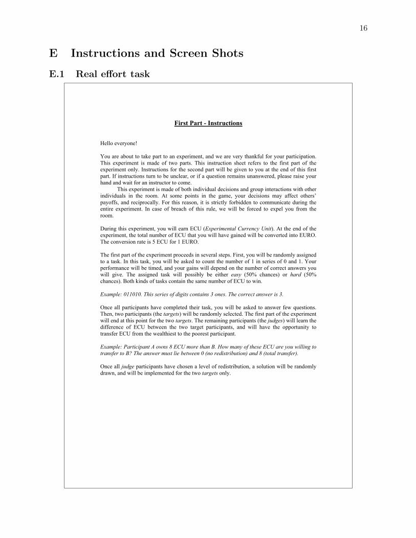
First Part - Instructions Hello everyone! You are about to take part to an experiment, and we are very thankful for your participation. This experiment is made of two parts. This instruction sheet refers to the first part of the experiment only. Instructions for the second part will be given to you at the end of this first part. If instructions turn to be unclear, or if a question remains unanswered, please raise your hand and wait for an instructor to come. This experiment is made of both individual decisions and group interactions with other individuals in the room. At some points in the game, your decisions may affect others’ payoffs, and reciprocally. For this reason, it is strictly forbidden to communicate during the entire experiment. In case of breach of this rule, we will be forced to expel you from the room. During this experiment, you will earn ECU (Experimental Currency Unit). At the end of the experiment, the total number of ECU that you will have gained will be converted into EURO. The conversion rate is 5 ECU for 1 EURO. The first part of the experiment proceeds in several steps. First, you will be randomly assigned to a task. In this task, you will be asked to count the number of 1 in series of 0 and 1. Your performance will be timed, and your gains will depend on the number of correct answers you will give. The assigned task will possibly be either easy (50% chances) or hard (50% chances). Both kinds of tasks contain the same number of ECU to win. Example: 011010. This series of digits contains 3 ones. The correct answer is 3. Once all participants have completed their task, you will be asked to answer few questions. Then, two participants (the targets) will be randomly selected. The first part of the experiment will end at this point for the two targets. The remaining participants (the judges) will learn the difference of ECU between the two target participants, and will have the opportunity to transfer ECU from the wealthiest to the poorest participant. Example: Participant A owns 8 ECU more than B. How many of these ECU are you willing to transfer to B? The answer must lie between 0 (no redistribution) and 8 (total transfer). Once all judge participants have chosen a level of redistribution, a solution will be randomly drawn, and will be implemented for the two targets only.

17

To sum up, the first part of the experiment unfolds as follows: 1) All participants are randomly assigned to a task; 2) All participants do their task; 3) Participants answer few questions; 4) Two participants are randomly selected (target participants); 5) The difference of ECU between the two targets is displayed to the judges who decide

on the allocation these ECU; 6) One redistribution proposal is randomly selected; 7) All participants learn their final payoff. It is equal to their performance to the task for

the judges, and equal to the performance affected by the randomly selected redistribution solution for the targets.

18

E.2 RSG: BASELINE

Second Part – Instructions (BASELINE) The second part of the experiment is about to start. In this part, you will be asked to complete a series of tasks. These tasks are substantially different from what you have done in the first part of this experiment. Your profit for each task will depend on both your effort (the number of ECU received at the task) and a random component (a positive or negative shock). At the beginning of this part, you will be randomly grouped with 3 other participants. Oncethegroupisformed, It will remain identical until the end of the experiment. Before the beginning of the second task, your group will be asked to choose a redistribution rule. The retained redistribution rule will be implemented after each task: it will determine the way to reallocate the sum of all profits made by the group at each period. Note that tasks are played individually. You will be asked to choose among the three following redistribution systems:

1) The libertarian rule corresponds to a situation without redistribution: each participant keeps the ECU he obtained at each task.

2) The egalitarian rule corresponds to a situation with full redistribution: all ECU obtained by the group members are reallocated in equal shares among group members.

3) The social-liberal corresponds to a situation with partial redistribution: all ECU obtained by the group members are reallocated proportionally to individual efforts.

Each participant will be asked to decide on the importance he wants to give to each of the three systems presented above to define the group redistribution system. One solution among the group members will then be randomly selected and implemented for the group until the end of the experiment. Example: One group of four participants obtained the following outcome at the assigned task: participant A, B and C obtained 4 ECU, while participant D, obtained 6 ECU. After a random shock participant A obtains 3 ECU and B, C and D obtain 5 ECU each.

Participant

Number of ECU obtained at the task

Number of ECU after the shock

Payoff if full libertarian redistribution system

Payoff if full social-liberal redistribution system

Payoff if full egalitarian redistribution system

A 4 3 3 4 4.5 B 4 5 5 4 4.5 C 4 5 5 4 4.5 D 6 5 5 6 4.5

19

E.3 RSG: EXTENDED

Second Part - Instructions (EXTENDED)

The second part of the experiment is about to start. In this part, you will be asked to complete a series of tasks. These tasks are substantially different from what you have done in the first part of this experiment. Your profit for each task will depend on both your effort (the number of ECU received at the task) and a random component (a positive or negative choc). Each task can give you individually 0, 4, 8, 12, 16 or 20 ECU. Individual shocks may affect your own payoff by the following amounts: -‐5, -‐4, -‐3, -‐2, -‐1, 0, +1, +2, +3, +4, +5 (all shocks have the same probability of occurrence). Shocks affecting other participants of your group are independent of the shock that affect your own payoff.

At the beginning of this part, you will be randomly grouped with 3 other participants. Once the group is formed, it will remain identical until the end of the experiment. Before the beginning of the second task, your group will be asked to choose a redistribution rule. The retained redistribution rule will be implemented after each task: it will determine the way to reallocate the sum of all profits made by the group at each period. Note that tasks are played individually.

You will be asked to choose among the three following redistribution systems:

1) The libertarian rule corresponds to a situation without redistribution: each participant keeps the ECU he obtained at each task and after the shock affected him.

2) The egalitarian rule corresponds to a situation with full redistribution: all ECU obtained by the group members after the individual shocks are reallocated in equal shares among group members.

3) The social-liberal system corresponds to a situation with partial redistribution: all ECU obtained by the group members after the individual shocks are reallocated proportionally to individual efforts (i.e. according to the individual pre-‐shock payoffs).

Each participant will be asked to decide on the importance he wants to give to each of the three systems presented above to define the group redistribution system. You will be able to give a score ranging from 0 to 10 to each of the three systems. These scores will define a redistribution system. For instance, if you allocate 8 points to each system, the corresponding redistribution rule will be made of 1/3 (one third) of the libertarian system, 1/3 of the egalitarian system, and 1/3 of the social-‐liberal system. If you decide to unequally weight the three systems, the resulting system will be proportional to the allocated scores. For example, if you allocate 8 points to the libertarian system, 4 points to the egalitarian system, and 0 point to the social-‐liberal system, the resulting redistribution system will be made of 2/3 (two thirds) of the libertarian system and 1/3 of the egalitarian system.

Once all group members will have made their choice, one and only one solution among the group members will be randomly drawn and implemented for the group until the end of the experiment. For instance, if one of your group member chose 20% of the libertarian system, 50% of the egalitarian system, and 30% of the social-‐liberal system, and that his/her solution has been selected to be implemented, the redistribution that will occur after each task will be made in the following proportions: 20% of the after-‐shock payoff will not be modified (20% libertarian), 50% will be redistributed equally

20

(50% egalitarian), and 30% will be redistributed proportionally to the pre-‐shock payoff (30% social-‐liberal).

Example: One group of four participants obtained the following outcomes at the assigned task: participant A, B and C obtained 4 ECU each, while participant D obtained 6 ECU (second column in the table below). After a random shock, participant A obtains 3 ECU, B and D obtain 5 ECU each, and C obtains 7 points (third column).

In the libertarian system, each individual keeps his/her own after-shock payoff. Individual A would therefore keep his/her 3 ECU (fourth column). In the egalitarian system, all individuals receive the same share of the total after-shock revenue, i.e. one fourth of 20 ECU. Individual A would therefore receive 5 ECU (fifth column). In the social-liberal system, participants receive a share proportional to their pre-shock payoff. Individual A received 4 ECU prior to the shock and the group totalized 18 ECU. The total revenue after the shock is 20 ECU. Using a rule of three, the payoff of individual A in a social-liberal system would be equal to: (4/18)*20=4.5 (rounded at 0.5) (sixth column).

Participant Number of ECU obtained at the task

Number of ECU after the shock

Payoff if full libertarian redistribution system

Payoff if full egalitarian redistribution system

Payoff if full social-liberal redistribution system

A 4 3 3 5 4.5

B 4 5 5 5 4.5

C 4 7 7 5 4.5

D 6 5 5 5 6.5

Somme 18 20 20 20 20

Imagine that the system that has been randomly selected to be implemented is as described in the above example: 20% libertarian, 50% egalitarian, and 30% social-liberal. The after-redistribution payoffs of individuals A, B, C and D are given in the table below. Participant A’s final payoff is computed by taking 20% of his/her libertarian payoff (0,20*3) (see above table), 50% of his/her egalitarian payoff (0,50*5), and 30% of his/her social-liberal payoff (0,30*4.5).

Participant Number of ECU after redistribution (before rounding)

Final payoff (rounded)

A 20% * 3 + 50%*5 + 30% * 4,5 = 0.6+2.5+1.35 = 4.45 4

B 20% * 5 + 50%*5 + 30% * 4,5 = 1+2.5+1.35 = 4.85 5

C 20% * 7 + 50%*5 + 30% * 4,5 = 1.4+2.5+1,35 = 5.25 5

D 20% * 5 + 50%*5 + 30% * 6,5 = 1+2.5+1.95 = 5.45 5

21

E.4 Screenshots

Figure E1: Screen Shot: Redistribution Decision in the Disinterested Dictator Game

Figure E2: Screen Shot: Control question for the RSG in the extended version. Partici-pants first calculate the payoffs for 100% libertarian, and then continue with the profits ofthe other systems.

Bruno Deffains, Romain Political Self-Serving Bias ... · Political Self-Serving Bias and...

Documents

Transcript of Bruno Deffains, Romain Political Self-Serving Bias ... · Political Self-Serving Bias and...