Brownian motion and gambling:from ratchets to paradoxical games

J.M.R. ParrondoLuis Dinıs

Grupo Interdisciplinar de Sistemas Complejos (GISC) andDept. de Fısica Atomica, Molecular y Nuclear,

Universidad Complutense de Madrid, 28040-Madrid, Spain.

October 26, 2003

Abstract

Two losing gambling games, when alternated in a periodic or randomfashion, can produce a winning game. This paradox has been inspired by cer-tain physical systems capable of rectifying fluctuations: the so-called Brow-nian ratchets. In this paper we review this paradox, from Brownian ratchetsto the most recent studies on collective games, providing some intuitive ex-planations of the unexpected phenomena that we will find along the way.

1 Introduction: A noisy revolution

Imagine two simple gambling games, say A and B, in which I play against you.Each one is a losing game for me, in the sense that my average capital is a de-creasing function of the number of turns we play. Once you are convinced that Ilose in both games, I give you a third proposal: alternate the games following thesequence AABBAABB... If you frown, the proposal can be modified to make itless suspicious: in each run we will randomly chose the game that is played. If youaccept either of these proposals you would have trusted your intuition too much,not realising that random systems may behave in an unexpected way.

The phenomenon we have just described is known as Parrondo’s paradox [1, 2,3]. It was originally inspired by a class of physical systems: the Brownian ratchets[4, 5, 6, 7, 8] and lately has received the attention of scientists working on severalfields, ranging from biology to economics. These are systems capable of rectifyingthermal fluctuations, such as those exhibited by a Brownian particle.

1

Brownian motion was one of the first crucial proofs of the discreteness of mat-ter. First observed by Jan Ingenhousz in 1785, and later rediscovered by Brownin 1828, the phenomenon consists on the erratic or fluctuating motion of a smallparticle when it is embedded in a fluid. In the beginning of the XXth century, Ein-stein realized that these fluctuations were a manifestation of the molecular natureof the fluid1 and devised a method to measure Avogadro’s number by using Brow-nian motion [9]. Since then, the study of fluctuations has been a major topic instatistical mechanics.

The theory of fluctuations helped to understand noise in electrical circuits, acti-vation processes in chemistry, the statistical nature of the second law of thermody-namics, and the origin of critical phenomena and spontaneous symmetry breaking,to cite only a few examples. In most of these cases, the role played by thermal fluc-tuations or thermal noise is either to trigger some process or to act as a disturbance.However, in the past two decades, the study of fluctuations has led to models andphenomena where the effect of noise is more complex and sometimes unexpectedand even counterintuitive.

Noise can enhance the response of a nonlinear system to an external signal,a phenomenon known as stochastic resonance [10]. It can create spatial patternsand ordered states in spatially extended systems [11, 12], and Brownian ratchetsshow that noise can be rectified and used to induce a systematic motion in a Brow-nian particle [4, 5, 6, 7, 8]. In these new phenomena, noise has a very differentrole from that considered in the past: it contributes to the creation of order. Thiscould be relevant in several fields, and specially in biology, since most biologicalsystems manage to keep themselves in ordered states even while surrounded bynoise, both thermal noise at the level of the cell and environmental fluctuations atthe macroscopic level.

However, fluctuations are not only restricted to physics, chemistry or biology.The origin of the theory of probability is closely related to gambling games, so-cial statistics, and even to the efficiency of juries [13]. Statistical mechanics andprobability theory have both contributed to each other and also to fields like eco-nomics. In 1900, five years before Einstein’s theory of the Brownian motion, theFrench mathematician Louis Bachelier worked out a theory for the price of a stockvery similar to Einstein’s [14]. Recently this link between probability, statisticalmechanics, and economics has crystallised in a new field: econophysics [15].

Some of the aforementioned constructive role of noise has been observed incomplex systems beyond physics. Stochastic resonance, for instance, has an in-creasing relevance in the study of perception and other cognitive processes [10, 16].

1The thermal origin of Brownian motion was firstly proposed by Delsaux in 1877 and later on byGouy in 1888 (see [9]).

2

Similarly, we expect that other elementary stochastic phenomena such as rectifica-tion will be observed in many situations not restricted to physics.

With this idea in mind, Parrondo’s paradox came up as a translation to simplegambling games of a Brownian ratchet discovered by Ajdari and Prost [4]. Theratchet was afterwards named by Astumian and Bier the flashing ratchet [6] andit was related to the idea proposed by Magnasco [5] that biological systems couldrectify fluctuations to perform work and systematic motion.

The paradox does not make use of Brownian particles, but only of the simplerfluctuations arising in a gambling game. However, it illustrates the mechanism ofrectification in a very sharp way, and for this reason we think that it could contributeto extend the “noisy revolution”, i.e., the idea that noise can create order, to thosefields where stochastic dynamics is relevant.

The paper is organised as follows. In section 2 we briefly review the flash-ing ratchet and explain how it can rectify fluctuations. Section 3 is devoted to theoriginal Parrondo’s paradox. There we introduce the paradoxical games as a dis-cretisation of the flashing ratchet, discuss an intuitive explanation of the paradoxthat we have called reorganisation of trends, and present an extension of the orig-inal paradox inspired by this idea. In section 4 we introduce several versions ofthe games involving a large number of players. Some interesting effects can beobserved in these collective games: redistribution of capital brings wealth [17],and collective decisions taken by voting or by optimizing the returns in the nextturn can lead to worse performance than purely random choices [18, 19]. Finally,in section 5 we briefly review the literature on the paradox and present our mainconclusions.

2 Ratchets

Here we revisit the flashing ratchet [4, 6], one of the simplest Brownian ratchetsand the most closely related to the paradoxical games. We refer to the exhaustivereview by Reimann on Brownian ratchets [7] or the special issue in Applied PhysicsA, edited by Linke [8], for further information on the subject.

Consider an ensemble of independent one-dimensional Brownian particles inthe asymmetric sawtooth potential depicted in Fig. 1. It is not difficult to show that,if the potential is switched on and off periodically, the particles exhibit an averagemotion to the right. Let us assume that the temperature T is low enough to ensurethat kT is much smaller than the maxima of the potential, and that we start withthe potential switched on and with all the particles around one of its minima, asshown in the upper plot of Fig. 1. When the potential is switched off, the particlesdiffuse freely, and the density of particles spreads as depicted in the central plot of

3

the figure. If the potential is then switched on again, each particle will move backto the initial minimum or to one of the nearest neighboring minima, depending onits position. Particles within the dark region will move to the right hand minimum,those within the small grey region will move to the left hand minimum, and thosewithin the white region will move back to their initial positions. As is apparentfrom the figure and due to the asymmetry of the potential, more particles fall intothe right hand minimum, and thus there is a net motion of particles to the right.For this to occur, the switching can be either random or periodic, but the averageperiod must be of the order of the time to reach the nearest barrier by free diffusion(see [4, 6] for details).

This motion can be seen as a rectification of the thermal noise associated withfree diffusion. The diffusion is symmetric: some particles move to the right andsome to the left, but their average position does not change. However, when thepotential is switched on again, most of the particles that moved to the left are drivenback to the starting position, whereas many particles that moved to the right arepushed to the right hand minimum. The asymmetric potential acts as a rectifier: it“kills” most of the negative fluctuations and “promotes” most of the positive ones.

The effect remains if we add a small force toward the left, i.e., in a directionopposite to the induced motion. In this case, the ratchet still induces a motionagainst the force. Consequently, particles perform work, and the system can beconsidered a Brownian motor. It can be proved that this type of motor is compatiblewith the second law of thermodynamics. In fact, the efficiency of such a motor isfar below the limits imposed by the second law [20, 21]. However, the ratchet witha force exhibits a curious property: when the potential is permanently on or off,the Brownian particles move in the same direction as the force, whereas they movein the opposite direction when the potential is switched on and off. This is theessence of the paradoxical games: we have two dynamics; in each one a quantity,namely the position of the Brownian particle, decreases in average; however, thesame quantity increases in average when the two dynamics are alternated.

3 Games

The flashing ratchet can be discretised in time and space, keeping most of its in-teresting features. The discretised version adopts the form of a pair of simplegambling games, which are the basis of the Parrondo’s paradox.

4

���������������������������������������������������������������������

����������������������������������������������������������������������������������������

� � � � � � � � � � � � � � � � � � � � � � � � � � � � � � � � � � �� � � � � � � � � � � � � � � � � � � � � � � � � � � � � � � � � � �� � � � � � � � � � � � � � � � � � � � � � � � � � � � � � � � � � �� � � � � � � � � � � � � � � � � � � � � � � � � � � � � � � � � � �� � � � � � � � � � � � � � � � � � � � � � � � � � � � � � � � � � �� � � � � � � � � � � � � � � � � � � � � � � � � � � � � � � � � � �� � � � � � � � � � � � � � � � � � � � � � � � � � � � � � � � � � �� � � � � � � � � � � � � � � � � � � � � � � � � � � � � � � � � � �� � � � � � � � � � � � � � � � � � � � � � � � � � � � � � � � � � �� � � � � � � � � � � � � � � � � � � � � � � � � � � � � � � � � � �� � � � � � � � � � � � � � � � � � � � � � � � � � � � � � � � � � �� � � � � � � � � � � � � � � � � � � � � � � � � � � � � � � � � � �� � � � � � � � � � � � � � � � � � � � � � � � � � � � � � � � � � �� � � � � � � � � � � � � � � � � � � � � � � � � � � � � � � � � � �� � � � � � � � � � � � � � � � � � � � � � � � � � � � � � � � � � �� � � � � � � � � � � � � � � � � � � � � � � � � � � � � � � � � � �� � � � � � � � � � � � � � � � � � � � � � � � � � � � � � � � � � �

����������������������������������������������������������������������������������������

� � � � � � � � � � � �� � � � � � � � � � � �� � � � � � � � � � � �� � � � � � � � � � � �� � � � � � � � � � � �� � � � � � � � � � � �� � � � � � � � � � � �� � � � � � � � � � � �� � � � � � � � � � � �� � � � � � � � � � � �� � � � � � � � � � � �� � � � � � � � � � � �� � � � � � � � � � � �� � � � � � � � � � � �� � � � � � � � � � � �� � � � � � � � � � � �� � � � � � � � � � � �� � � � � � � � � � � �� � � � � � � � � � � �� � � � � � � � � � � �� � � � � � � � � � � �

�������������������������������������������������

ON

ON

OFF

Figure 1: The flashing ratchet at work. The figure represent three snapshots ofthe potential and the density of particles. Initially (upper figure), the potentialis on and all the particles are located around one of the minima of the potential.Then the potential is switched off and the particles diffuse freely, as shown in thecentered figure, which is a snapshot of the system immediately before the potentialis switched on again. Once the potential is connected again, the particles in thedarker region move to the right hand minimum whereas those within the smallgrey region move to the left. Due to the asymmetry of the potential, the ensembleof particles move, in average, to the right.

5

No Yes

Game A Game B

win lose

1/2-ε

Is X(t) a multiple of three?

win lose

1/2+ε

win lose

3/4-ε 1/4+ε 1/10-ε 9/10+ε

Figure 2: Rules of the paradoxical games. In game A, the player wins (her capitalincreases by one euro) with a probability 1/2 − ε and loses (her capital decreasesby one euro) with a probability 1/2 + ε, ε being a small positive number. In thefigure, these probabilities are represented by a coin with two possible outcomes. Ingame B, the probability to win and lose depends on the capital X(t) of the player:if X(t) is a multiple of three, then we use a “bad” coin, with a probability to winequal to 1/10 − ε; if X(t) is not a multiple of three, then a “good” coin, with aprobability to win equal to 3/4− ε, is used. In the figure the darkness of the coinsrepresents their “badness” for the player.

3.1 The original paradox

We consider two games, A and B, in which a player can make a bet of 1 euro.X(t) denotes the capital of the player, where t = 0, 1, 2 . . . stands for the numberof turns played. Game A consists of tossing a slightly biased coin so that the playerhas a probability pA of winning which is less than a half. That is, pA = 1/2 − ε,where the bias ε is a small positive number.

The second game, B, is played with two biased coins, a “bad coin” and a “goodcoin”. The player must toss the bad coin if her capital X(t) is a multiple of 3, theprobability of winning being pbad = 1/10 − ε. Otherwise, the good coin is tossedand the probability of winning is pgood = 3/4− ε. The rules of games A and B arerepresented in Fig. 2, in which the darkness represents the “badness” of each coin.

For these choices of pA, pgood and pbad, both games are fair if ε = 0, in thesense that 〈X(t)〉 is constant. This is evident for game A, since the probabilities towin and lose are equal. The analysis of game B is more involved, but we will soonprove that the effect of the good and the bad coins cancel each other for ε = 0.

On the other hand, both games have a tendency to lose if ε > 0, i.e., 〈X(t)〉

6

800 20 40 60 100

-1

0

1

2

Turns played

[3,2]

[2,2]

[4,4]

A

B

random

<X(t)>

Figure 3: Average capital for 5000 players as a function of the number of turnsfor game A, B and their periodic and random combinations. ε = 0.005 and [a, b]stands for periodic sequences where A (B) is played a (b) consecutive turns.

decreases with the number of turns t. Surprisingly enough, if the player randomlychooses the game to play in each turn, or plays them following some predefinedperiodic sequence such as ABBABB..., then her average capital 〈X(t)〉 is an in-creasing function of t, as can be seen in Fig. 3.

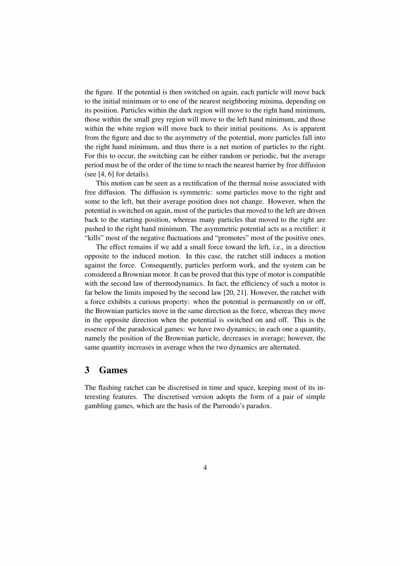
The paradox is closely related to the flashing ratchet. If we visualise the capitalX(t) as the position of a Brownian particle in a one dimensional lattice, game A,for ε = 0, is a discretisation of the free diffusion, whereas game B resembles themotion of the particle under the action of the asymmetric sawtooth potential. Fig.4 shows this spatial representation for game B compared with the ratchet potential.When the particle is on a dark site, the bad coin is used and the probability to winis very low, whereas on the white sites the most likely move is to the right. Thesawtooth potential has a short spatial interval in which the force is negative anda long interval with a positive force. Equivalently, game B uses a bad coin on a“short interval”, i.e., on one site of every three on the lattice, and a good coin ona “long interval” corresponding to two consecutive sites which are not multiple ofthree (see Fig. 4).

As in the flashing ratchet, game B rectifies the fluctuations of game A. Supposethat we play the sequence AABBAABB... and that X(t) is a multiple of threeimmediately after two instances of game B. Then we play game A twice, whichcan drive the capital back to X(t) or to X(t) ± 2. In the latter case, the next turnis for game B with a capital that is not a multiple of three, which means a goodchance of winning. That is, game B rectifies the fluctuations that occurred in the

7

-1 1 2 65430

Figure 4: A random walk picture of game B compared with the ratchet potential.The bad coin (black dots) plays the role of the negative force acting on a shortinterval, whereas the two consecutive good coins (white dots) are the analogous ofthe positive force acting on the long intervals.

two turns of game A. The rectification is not as neat as in the low temperatureflashing ratchet, but enough to cause the paradox.

There is a more rigorous way of associating a potential to a gambling game byusing a master equation [22]. However, it provides a similar picture of game B, asa random walk that is nonsymmetric under inversion of the spatial coordinate andcapable of rectifying fluctuations.

3.2 Reorganisation of trends

Beside the ratchet effect, one can explain the paradox considering another interest-ing mechanism. Recall that game B is played with two coins: a good one, usedwhenever the capital of the player is not a multiple of three, and a bad one which isused when the capital is a multiple of three. Therefore, the “profitability” of gameB crucially depends on how often the bad coin is used, i.e., on the probability π0

that the capital is a multiple of three. It turns out that, when game B is played,this probability is not 1/3, as one could naively expect, but larger. This can bereasoned from figure 4. When the capital is at a white site, its most likely move isto the right, whereas at dark sites the most likely move is to the left. The capitalthus spends more time jumping forth and back between a multiple of three and itsleft hand neighbour than what would do if it moved completely at random. Con-sequently, the probability π0 is larger than 1/3. On the other hand, under game Athe capital does move in a random way. Therefore, playing game A in some turnsshifts π0 towards 1/3, or, equivalently, reduces the number of times the bad coin ofgame B is used. In other words, game A, although losing, boosts the effect of thegood coin in B, giving the overall game a winning tendency. We have named thismechanism reorganization of trends, since game A reinforces the positive trendalready present in game B.

Along this section, we formulate this argument in a quantitative way. Let us

8

first consider game B separately. The probability to win in the t-th turn can becalculated as

pwin(t) = π0(t)pbad + [1− π0(t)] pgood (1)

where π0(t) is the probability of X(t) being a multiple of 3 (i.e. of using the badcoin).

One can calculate the value of π0(t), by using very simple techniques from thetheory of Markov chains. First, we define the random process

Y (t) ≡ X(t) mod 3 (2)

taking on only three possible values or states, Y (t) = 0, 1, 2, depending on whetherthe capital X(t) is a multiple of three, a multiple of three plus one, or a multipleof three plus two, respectively. This variable Y (t) is a Markov process, i.e., thestatistical properties of Y (t+ 1) depend only on the value taken on by Y (t). Thisallows one to derive a master equation for its probability distribution.

Let π0(t), π1(t), π2(t) be the probability that Y (t) is equal to 0, 1, and 2, re-spectively. There are two possibilities for Y (t) = 2 to occur: either Y (t− 1) = 0and we lose in the t-th turn (with probability 1 − pbad), or Y (t − 1) = 1 and wewin in the t-th turn (with probability pgood). Therefore:

π2(t) = (1− pbad)π0(t− 1) + pgoodπ1(t− 1). (3)

Following the same type of argument, one can derive equations for π0(t) andπ1(t), and the three equations can be written in matrix form as:

~π(t) = ΠB~π(t− 1) (4)

where

~π(t) ≡

π0(t)π1(t)π2(t)

(5)

and

ΠB ≡

0 1− pgood pgood

pbad 0 1− pgood

1− pbad pgood 0

. (6)

After a small number of turns of game B, ~π(t) approaches to a stationary value~πst

B , which is invariant under the transformation given by Eq. (4), i.e.:

~πstB = ΠB~π

stB . (7)

9

The third component of the solution of this equation reads:

πst0B =

5

13−440

2197ε+O(ε2) ' 0.38− 0.20 ε (8)

where we have used the values of the original paradox, pbad = 1/10 − ε andpgood = 3/4− ε, and have expanded the solution up to first order of ε, to simplifythe exposition.

Substituting this value in Eq. (1) we obtain the probability of winning for gameB for sufficiently large t

pwin,B =1

2−147

169ε+O(ε2) (9)

which is less than 1/2 for ε > 0. This proves that game B is fair for ε = 0 andlosing for ε > 0, as shown in Fig. 3.

The paradox arises when game A comes into play. Game A is always playedwith the same coin, regardless of the value of the capital X(t), and therefore drivesthe probability distribution ~π(t) to a uniform distribution. Thus, game A makesπ0(t) tend to 1/3. Since 1/3 < πst

0B, the effect of game A is to decrease theprobability of using the bad coin in the turns where B is played.

This can be seen in a more precise way, since the random combination of gamesA and B can be again solved by using the master equation:

~πstAB =

1

2[ΠB +ΠA]~π

stAB (10)

where

ΠA =

0 1− pA pA

pA 0 1− pA

1− pA pA 0

(11)

with pA = 1/2− ε. The probability of using the bad coin decreases to

πst0AB =

245

709−48880

502681ε+O(ε2) ' 0.35− 0.10 ε. (12)

The probability of winning in this randomised combination of games A and B is

pwin,AB = πst0AB

pbad + pA

2+[

1− πst0AB

] pgood + pA

2

=727

1418−486795

502681ε+O(ε2) (13)

which is greater than 1/2 for a sufficiently small ε.

10

This is the mechanism behind the paradox which we have termed “reorgani-sation of trends”: although game A consists itself in a negative trend because ituses a slightly bad coin, it increases the probability of using the good coin of B,i.e., game A reinforces the positive trend already present in B enough to make thecombination win.

Periodic sequences can also be studied as Markov chains and their probabilityof winning in a whole period can be easily computed using different combinationsof the matrices ΠA and ΠB . Finally, the slopes of the curves in Fig. 3 can becalculated as 〈X(t+ 1)〉 − 〈X(t)〉 = 2pwin − 1.

3.3 Capital-independent games

The modulo rule in game B is quite natural in the original representation of thegames as a Brownian ratchet. However, the rule may not suit some applications ofthe paradox to biology, biophysics, population genetics, evolution, and economics.Thus, it would be desirable to devise new paradoxical games based on rules inde-pendent of the capital. Parrondo, Harmer and Abbott introduced such a game inRef. [23], inspired by the reorganisation of trends explained in the last section.

In the new version, game A remains the same as before, but a game B′, whichdepends on the history of wins and losses of the player, is introduced. Game B′ isplayed with four coins B′

1, B′

2, B′

3, B′

4 following history-based rules explained intable 1.

Before last Last Coin Prob. of win Prob. of losst− 2 t− 1 at t at t at tLoss Loss B′

1 p1 1− p1

Loss Win B′

2 p2 1− p2

Win Loss B′

3 p3 1− p3

Win Win B′

4 p4 1− p4

Table 1: History-based rules for game B’

The paradox reappears, for instance, when setting p1 = 9/10 − ε, p2 = p3 =1/4− ε, and p4 = 7/10− ε. With these numbers and for ε small and positive, B′ isa losing game, while either a random or a periodic alternation of A and B′ producesa winning result. Fig. 5 shows a theoretical computation of the average capital forthese history-dependent paradoxical games.

The paradox is reproduced because there are bad coins in game B′ which areplayed more often than in a completely random game, i.e., a quarter of the time.

11

0 20 40 60 80 100-0.8

-0.4

0

0.4

0.6

Turns played

Cap

ital

random

[2,2]

A

B'

Figure 5: Average capital as a function of the number of turns in the capital inde-pendent games. We plot the result for game A and B′, as well as for the randomcombination and the periodic sequence AAB′B′... In all the cases, ε = 0.003.

For the above choices of pi, i = 1, 2, 3, 4, the bad coins are B ′

2 and B′

3. The othertwo coins, B′

1 and B′

4, are good coins.Due to the fact that game B′ rules depend on the history of wins and losses, the

capital X(t) is no longer a Markovian process. However, the random vector

Y (t) =

(

X(t)−X(t− 1)X(t− 1)−X(t− 2)

)

(14)

can take on four different values and is indeed a Markov chain. The transitionprobabilities are again easily obtained from the rules of game B′ and an analyt-ical solution can be obtained following a similar argument as in section 3.2 (seehowever Ref. [23] for details).

We see that the mechanism that we have called reorganisation of trends canbe used to extend the paradox to other gambling games. It is also noteworthy thatthe price we must pay to eliminate the dependence on the capital in the originalparadox is to consider history-dependent rules, i.e., games where the capital is nolonger Markovian.

4 Collective games

In this section we analyse three different versions of paradoxical games played bya large number of individuals. The three share the feature that it can sometimes be

12

better for the players to sacrifice short term benefits for higher returns in the future.

4.1 Capital redistribution brings wealth.

Reorganisation of trends tells us that the essential role of game A in the paradox isto randomise the capital and make its distribution more uniform. Toral has foundthat a redistribution of the capital in an ensemble of players has the same effect[17].

In the new paradoxical games introduced by Toral in [17], there are N playersand one of them is randomly selected in each turn. They can play two games.The first one, game A’, consists of giving a unit of his capital to another randomlychosen player in the ensemble, that is, game A′ is nothing but a redistribution of thetotal capital. The second one, game B, is the same as in the original paradox. Undergame A′ the capital does not change, where game B is, as before, a losing game.The striking result is that the random combination of the two games is winning,i.e., the redistribution of capital performed in the turns where A′ is played turns thelosing game B into a winning one, actually increasing the total capital available.Thus, the redistribution of capital turns out to be beneficial for everybody. Thiseffect is shown in Fig. 6 where the average total capital in a simulation with 10players and 500 realizations is depicted for games B and A′, and for their randomcombination. It is remarkable that the effect is still present when the capital isrequired to flow from richer to poorer players (see [17] for details).

The explanation to this phenomenon follows the same lines as in the originalparadox.

4.2 Dangerous choices I: The voting paradox

Up to now, we have considered sequences of games that are “imposed” to the playeror players. Either they play game A, game B, or a periodic or random sequence,but we never allow the players to choose the game to be played in each turn. Inthe case of a single player this deference is quite generous, since her capital wouldincrease in average under the following trivial choice: she selects game B if hercapital is not a multiple of three and game A otherwise. This is undoubtedly thebest strategy, because the best coin is always used in every turn. Moreover, it isnot difficult to see that this choice strategy performs much better than any otherrandom or periodic combination of games.

However, things change when we consider an ensemble of players. How canthe ensemble choose the game to be played in each turn? There are some pos-sibilities, such as letting them vote for the preferred game or trying to maximisethe winning probability in each turn. Which is then the best choice strategy? We

13

0 1000 2000 3000 4000 5000-10

-6

-2

0

2

6

10

Turns played

Ave

rage

cap

ital

random

A'

B

Figure 6: Average capital per player as a function of the number of turns in gameB, game A′ (redistribution of capital), and the random combination. The data havebeen obtained for ε = 0.01, simulating an ensemble of 10 players and averagingover 500 realizations.

will see that the paradoxical games also yield some surprises in this context: thechoice that prefers the majority of the ensemble turns to be worse than a random orperiodic combination of games. Even if we select the game maximising the profitin every turn, we can end with systematic loses, as shown in the next section.

Consider a set of N players who play game A or B against a casino. In eachturn, all of them play the same game. Therefore, they have to make a collectivedecision, choosing between game A or B in each turn. We will firstly use a majorityrule to select the game, that is, the game which receives more votes is played byall the players simultaneously. The vote of each player will be determined by hercapital, following the strategy that we have explained above for a single player.Players with capital multiple of three will vote for game A, whereas the rest willvote for B.

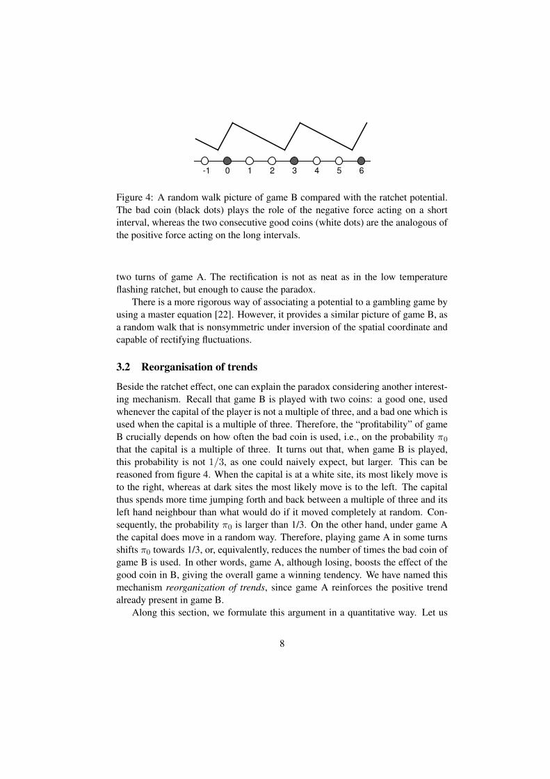
This strategy, which is optimal for a single player, turns to be losing if thenumber of players is large enough [19]. This is shown in figure 7, where we plotthe average capital in an ensemble with an infinite number of players. On the otherhand, if the game is selected at random the capital increases in time.

In order to explain this behaviour, we will focus on the evolution of π0(t), thefraction of players whose capital is a multiple of three. The selection of the gameby voting can be rephrased in terms of π0(t). As mentioned above, every playervotes for the game which offers him the higher probability of winning according

14

to his own state. Then, every player whose capital is a multiple of three will votefor game A in order to avoid the bad coin in B. That accounts for a fraction π0(t)of the votes. The remaining fraction 1− π0(t) of the players will vote for game Bto play with the good coin. Since the majority rule establishes that the game whichreceives more votes is selected, game A will be played if π0(t) > 1/2. Conversely,the whole set of players will play game B when π0(t) is below 1/2.

On the other hand, as we have seen in section 3.2, playing game B makes π0(t)tend to a stationary value given by Eq. (8), namely, πst

0B ' 0.38 − 0.2ε < 1/2for ε > 0, whereas playing game A makes π0 tend to 1/3. This is still valid forthe present model, since the N players only interact when they make the collectivedecision, otherwise they are completely independent.

If π0(t) > 1/2, then the ensemble of players will select game A. The fractionπ0(t) will decrease until it crosses this critical value 1/2. At that turn, B is theselected game and it will remain so as long as π0 does not exceed 1/2. However,this can never happen, since game B drives π0 closer and closer to πst

0B which isbelow 1/2. Hence, after a number of turns, the system gets trapped playing gameB forever with π0 asymptotically approaching πst

0B. Since ε is positive, game B isa losing game (c.f. section 3.2) and, therefore, the majority rule yields systematiclosses, as can be seen in Fig. 7. We have also plotted in Fig. 8 the fraction π0(t), tocheck that, once π0(t) crosses 1/2, game B is always chosen and π0(t) approachesπst

0B, staying far below 1/2.On the other hand, if, instead of using the majority rule, we select the game

at random or following a periodic sequence, game A will be chosen even thoughπ0 < 1/2. This is a bad choice for the majority of the players, since playing Bwould make them toss the good coin. That is, the random or periodic selection willcontradict from time to time the will of the majority. Nevertheless, choosing thegame at random keeps π0 away from πst

0B, as shown in Fig. 8, i.e., in a region wheregame B is winning (π0 < πst

0B). Therefore, the random choice yields systematicgains, as shown in Fig. 7.

It is worth noting that choosing the game at random is exactly the same as ifevery player voted at random. Therefore, the players get a winning tendency whenthey vote at random whereas they lose their capital when they vote according totheir own benefit in each run.

4.3 Dangerous choices II: The risks of short-range optimisation

Yet another “losing now to win later” effect can be observed in the collective para-doxical games with another choice strategy. As in the previous example, we con-sider a large set of players, but we have to add a small ingredient to achieve thedesired effect: now only a randomly selected fraction γ of them play the game in

15

0 10 20 30 40 50 60-0.6

-0.4

-0.2

0

0.2

0.4

0.6

0.8

1

Turns played

Ave

rage

cap

ital

MR

random

Figure 7: Average capital per player in the collective games as a function of thenumber of turns, when the game is selected at random and following the prefer-ence of the majority of the players (MR). Notice that, in the stationary regime,the majority rule (MR) yields systematic loses whereas the random choice winsin average. These are analytical results with ε = 0.005 and an infinite number ofplayers.

each turn. Suppose we know the capital of every player so we can compute whichgame, A or B, will give the larger average payoff in the next turn. Again, and evenmore strikingly, selecting the “most favorable game” results in systematic losseswhereas choosing the game at random or following a periodic sequence steadilyincreases the average capital [18].

The knowledge of the capital of every player allows us to choose the game withthe highest average payoff in the next turn, since this optimal game can easily beobtained from the fraction π0(t) of players whose capital is a multiple of three.These individuals will play the bad coin if game B is chosen and the remainingfraction 1 − π0(t) will play the good coin. Hence, the probability of winning forgame B reads

pwinB = π0pbad + (1− π0)pgood. (15)

In case game A is selected, the probability to win is pwinA = pA = 1/2− ε for alltime t. Therefore, to choose the game with the larger payoff 〈X(t+1)〉−〈X(t)〉 =2pwin − 1 in every turn t, we must

play A if pwinA ≥ pwinB(π0)

play B if pwinA < pwinB(π0) (16)

16

0 10 20 30 40 50

0.1

0.2

0.3

0.4

Turns played

MRRandom

π0Bst

1/2

π0Ast

π (t)0

Figure 8: The fraction of players π0(t) with capital multiple of three as a functionof time when the game is chosen at random and following the majority rule (MR).In both cases, ε = 0.005 and N = ∞. The horizontal lines indicate the thresholdvalue for the majority rule (1/2), and the stationary values for games A and B, πst

0A

and πst0B, respectively. The figure clearly shows that the random strategy keeps

π0(t) small, whereas the majority rule, selecting B most of the time, drives π0(t)to a value where both game A and B are losing.

17

0 20 40 60 80 100-0.5

0

0.5

1

1.5

Turns played

Ave

rage

cap

ital

SR optimalABBABB...Random

Figure 9: Average capital as a function of time for the three different strategiesexplained in the text, with N =∞, γ = 0.5, and ε = 0.005. The short-range (SR)optimal strategy is losing in the stationary regime, whereas the two blind strategies:choosing the game to be played either at random or following the periodic sequence(ABBABB...), yield a systematic gain.

or equivalently

play A if π0(t) ≥ π0c

play B if π0(t) < π0c (17)

with π0c ≡ (pA − pgood)/(pA − pbad) = 5/13. We will call this way of selectingthe game the short-range optimal strategy. We will also consider that the gameis selected following either a random or periodic sequence. These are both blindstrategies, since they do not make any use of the information about the state of thesystem. However, and surprisingly enough, they turn out to be much better thanthe short-range optimal strategy, as shown in Fig. 9.

Notice that (17) is similar to the way the game is selected by the majorityrule considered in the previous section, but replacing 1/2 by the new critical valueπ0c = 5/13. Therefore, the explanation of this model goes quite along the samelines as for the voting paradox, although with some differences. Unlike 1/2, π0c

equals the stationary value of π0(t) for game B when ε = 0. As in the votingparadox, game A drives π0 below π0c because game A makes π0 tend to 1/3. Ifπ0(t) < π0c, then game B is played, but π0(t + 1) will be still below π0c only for

18

20 40 60 80 1000.3

0.32

0.34

0.36

0.38

0.4

0.42

0.44

0.46

Turns played

SR optimalABBABB...Random

A

π0Ast

π0Bst

π (t)0

Figure 10: The fraction π0(t) of players with capital multiple of three as a functionof the number of turns, for ε = 0, N =∞, and γ = 0.5. The horizontal lines showthe stationary values for game A and game B (which coincides with the criticalfraction π0c for the short-range optimal strategy). As we have in figure 8 with themajority rule, the short-range optimal strategy drives π0(t) towards higher valuesthan the other two strategies.

γ sufficiently small. For example, if γ = 1/2 and ε = 0, game B is chosen fortytimes in a row before switching back to game A, making π0 become approximatelyequal to πst

0B at almost every turn. This behaviour is shown in Fig. 10. As long asπ0 is close to πst

0B, the average capital remains approximately constant, as shownin Fig. 11.

In contrast, the periodic and random strategies choose game A with π0 < π0c.Although this does not produce earnings in that turn, it keeps π0 away from πst

0B.When game B is chosen again, it has a large expected payoff since π0 is not closeto πst

0B. By keeping π0 not too close to πst0B, the blind strategies perform better than

the short-range optimal prescription, as can be seen in Fig. 11.The introduction of ε > 0 has two effects. First of all, it makes πst

0B decreaseby a small amount, as indicated in Eq. (8). This makes it even more difficult forthe short-range optimal strategy to choose game A, and after a few runs game Bis always selected. Since game B is now a losing game, the short-range optimalstrategy is also losing whereas periodic and random strategies keep their winningtendency, as can be seen in Fig. 9.

To summarise, the short-range optimal strategy chooses B most of the time,

19

0 20 40 60 80 100-0.5

0

0.5

1

1.5

2

Turns played

Ave

rage

cap

ital

SR optimalABBABB...Random

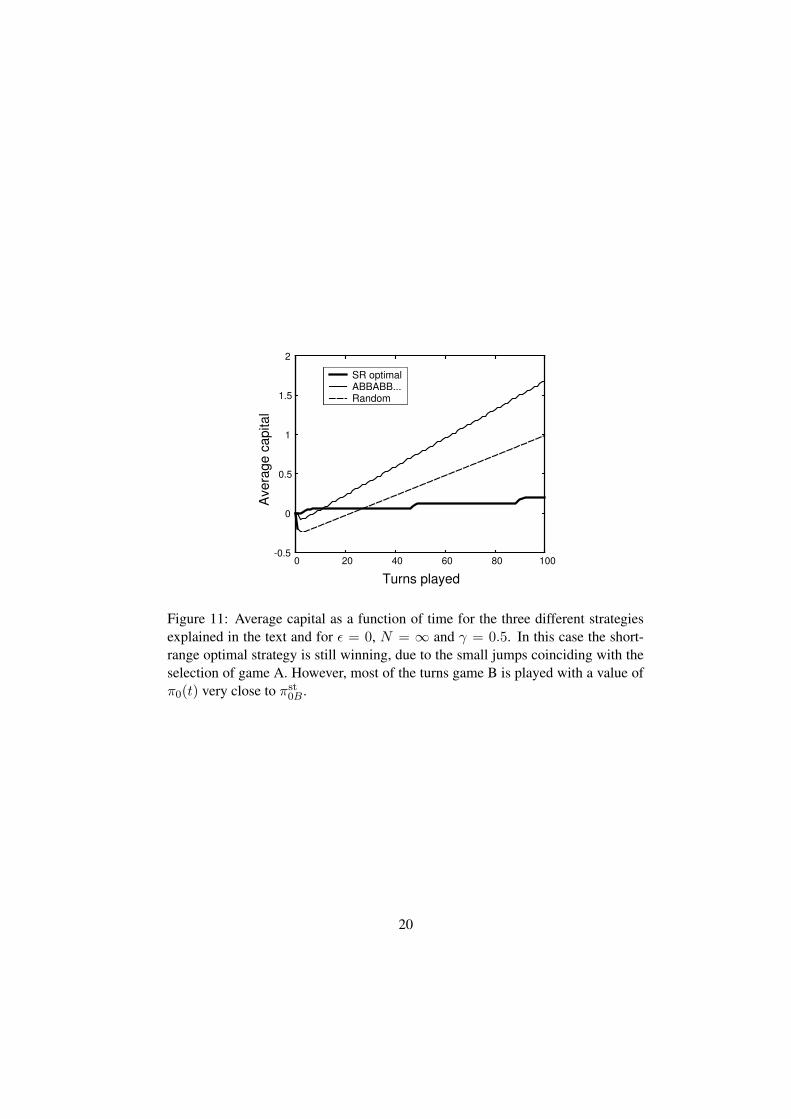
Figure 11: Average capital as a function of time for the three different strategiesexplained in the text and for ε = 0, N = ∞ and γ = 0.5. In this case the short-range optimal strategy is still winning, due to the small jumps coinciding with theselection of game A. However, most of the turns game B is played with a value ofπ0(t) very close to πst

0B.

20

since it is the game which gives the highest returns in each turn. However, thischoice drives π0(t) to a region in which B is no longer a winning game. On theother hand, the random strategy from time to time sacrifices the short term returnsby selecting game A, but this choice keeps the system in a “productive region”. Wecould say that the short-range optimal strategy is “killing the goose that laid thegolden eggs”, an effect that is also present in simple deterministic systems [18].

5 Conclusions

We have presented the original Parrondo’s paradox and several examples showinghow the basic mechanisms underlying the paradox can yield other counter-intuitivephenomena. We finish by reviewing these mechanisms as well as the literaturerelated with the paradox.

The first mechanism, the ratchet effect, occurs when fluctuations can help tosurmount a potential barrier or a “losing streak”. These fluctuation can either comefrom another losing game, such as in the original paradox, from a redistributionof the capital, such as in Toral’s collective games [17], or from a purely diffusivemotion, such as in the flashing ratchet.

A second mechanism is the reorganisation of trends, which occurs when gameA reinforces a positive trend already present in game B. The same mechanism canbe observed in the games with capital independent rules and it helps to understandthe counter-intuitive behaviour of the collective games presented in section 4.2 and4.3, where random choices perform better than the choice preferred by the majorityor the one optimizing short term returns. These models also prompt the questionof how information can be used to design a strategy. It is a relevant question forcontrol theory and also for statistical mechanics, since the paradox is a purely col-lective effect that goes away for a single player, i.e., the choices following theshort-range optimal strategy and the majority rule perform much better than therandom or periodic ones.

There is a third mechanism which we have not addressed along the paper, butimmediately arises if we consider the games as dynamical systems: the outcome ofan alternation of dynamics can always be interpreted as a stabilization of transientstates. This interpretation has allowed some authors to extend the basic messageof the paradox to pattern formation in spatially extended systems [24, 25, 26, 27].In these papers, a new mechanism of pattern formation based on the alternationof dynamics is introduced. They show how the global alternation of two dynam-ics, each of which leads to a homogeneous steady state, can produce stationary oroscillatory patterns upon alternation.

Another interesting application of the stabilization of transient states is pre-

21

sented in Ref. [28]. Two dynamics for the population of a virus are introducedwith the following property: in each dynamics, the population vanishes, whereasthe alternation of the two dynamics, whose origin could be the seasonal variation,induces an outbreak of the virus.

Similar effects can be seen in quantum systems. Lee et al. have devised atoy model in which the alternation of two decoherence dynamics can significantlydecrease the decoherence rate of each separate dynamics [29]. Also in the quantumdomain, the paradox has received some attention: there have been some proposalsof a quantum version of the games [30, 31] closely related with the recent theoryof quantum games [32], and the paradox has been reproduced in the contexts ofquantum lattice gases [33] and quantum algorithms [34].

To finish this partial account of the existing literature on the paradox, we men-tion the work by Arena et al [35], who analyse the performance of the games usingchaotic instead of random sequences of choices; that of Chang and Tsong [36],who study the hidden coupling between the two games in the paradox and presentseveral extensions even for deterministic dynamics; and the paper by Kocarev andTasev [37], relating the paradox with Lyapunov exponents and stochastic synchro-nisation.

In summary, Parrondo’s paradox has drawn the attention of many researchersto non-trivial phenomena associated with switching between two dynamics. Wehave tried to reveal in this paper some of the basic mechanisms that can yieldan unexpected behaviour when switching between two dynamics, and how thesemechanisms work in several versions of the paradox. As mentioned in the intro-duction, we believe that the paradox and its extensions are contributing to a deeperunderstanding of stochastic dynamical systems. In the case of statistical mechan-ics, switching is in fact a source of non-equilibrium which is ubiquitous in nature,due to day-night or seasonal variations [28]. Nevertheless, it has not been studiedin depth until the recent introduction of ratchets and paradoxical games. As theparadox suggests, we will probably see in the future new models and applicationsconfirming that noise and switching, even between equilibrium dynamics, can be apowerful combination to create order and complexity.

Acknowledgements

We thank valuable comments on the original manuscript made by Katja Linden-berg, Javier Buceta, Martin Plenio, and H. Leonardo Martınez. This work wassupported by a grant from the New Del Amo Program (U.C.M.), and by MCYT-Spain Grant BFM 2001-0291.

22

References

[1] G.P. Harmer and D. Abbott, Stat. Sci. 14, 206 (1999).

[2] G.P. Harmer and D. Abbott, Nature 402, 846 (1999).

[3] G.P. Harmer and D. Abbott, Fluct. Noise Lett. 2, R71 (2002).

[4] A. Ajdari and J. Prost, C.R. Acad. Sci. Paris II, 315, 1635 (1993).

[5] MO Magnasco, Phys. Rev. Lett. 71, 1477 (1993).

[6] R.D. Astumian and M. Bier, Phys. Rev. Lett. 72, 1766 (1994).

[7] P. Reimann, Phys. Rep. 361, 57 (2002).

[8] H. Linke, Appl. Phys. A 75, 167 (2002).

[9] A. Einstein, Investigations on the Theory of Brownian Movement (Dover,New York, 1956).

[10] L. Gammaitoni, P. Hanggi, P. Jung, and F. Marchesoni, Rev. Mod. Phys. 70,223–288 (1998).

[11] C. Van den Broeck, J.M.R. Parrondo, and R. Toral, Phys. Rev. Lett. 73, 3395(1994).

[12] J. Garcıa-Ojalvo and J.M. Sancho, Noise in Spatially Extended Systems(Springer-Verlag, New York, 1999).

[13] I. Hacking, The Taming of Chance (Cambridge University Press, Cambridge,1990).

[14] L. Bachelier. Theorie de la Speculation (Thesis) Annales Scientifiques del’Ecole Normale Superieure, I I I -17, 21-86 (1900).

[15] R.N. Mantegna and H.E. Stanley, An Introduction to Econophysics Correla-tions and Complexity in Finance (Cambridge University Press, Cambridge,2000).

[16] T. Mori and S. Kai, Phys. Rev. Lett. 88, 218101(2002).

[17] R. Toral, Fluct. Noise Lett. 2, L305 (2002).

[18] L. Dinis and J.M.R. Parrondo, Europhys. Lett. 63, 319 (2003).

23

[19] L. Dinis and J.M.R Parrondo, Inefficiency of voting in Parrondo games. Sub-mitted.

[20] J.M.R. Parrondo and B.J. Cisneros, Appl. Phys. A 75, 179 (2002).

[21] J.M.R. Parrondo, J.M. Blanco, F.J. Cao, and R. Brito, Europhys. Lett. 43, 248(1998).

[22] R. Toral, P. Amengual, and S. Mangioni, Physica A 327, 105 (2003).

[23] J.M.R. Parrondo, G.P. Harmer, and D. Abbott, Phys. Rev. Lett., 84 5526(2000)

[24] J. Buceta, K. Lindenberg, and J. M. R. Parrondo, Phys. Rev. Lett. 88, 024103(2002).

[25] J. Buceta, K. Lindenberg, and J. M. R. Parrondo, Phys. Rev. E 66, 036216(2002); ibid 069902(E).

[26] J. Buceta, K. Lindenberg, and J. M. R. Parrondo, Fluct. Noise Lett. 2, R139(2002).

[27] J. Buceta and K. Lindenberg, Phys. Rev. E 66, 046202 (2002).

[28] C. Escudero, J. Buceta, F.J. de la Rubia, and K. Lindenberg, Outbreaks ofHantavirus induced by seasonality, cond-mat/0303596.

[29] C.F. Lee, N. F. Johnson, F. Rodrıguez, and L. Quiroga, Fluct. Noise Lett. 2,L293 (2002).

[30] A.P. Flitney, J. Ng, and D. Abbott, Physica A 314, 35 (2002).

[31] D.A. Meyer and H. Blumer, Fluct. Noise Lett. 2, L257 (2002).

[32] J. Eisert, M. Wilkens, and M. Lewenstein, Phys. Rev. Lett. 83, 3077 (1999).

[33] D.A. Meyer and H. Blumer, J. Stat. Phys. 107, 225 (2002).

[34] C.F. Lee and N. F. Johnson. Parrondo Games and Quantum Algorithms,quant-ph/0203043.

[35] P. Arena, S. Fazzino, L. Fortuna, and P. Maniscalco, Chaos Solitons and Frac-tals 17, 545 (2003).

[36] C.H. Chang and T.Y. Tsong, Phys. Rev. E 67 025101 (2003).

[37] L. Kocarev and Z. Tasev Z, Phys. Rev. E 65, 046215 (2002).

24

Biographies

Juan M.R. Parrondo studied in the Universidad Complutense de Madrid (Spain)where he obtained both his Major (1987) and his PhD (1992) in Physics. Heworked as postdoc in the University of California, San Diego (USA) and in theLimburgs Universitair Centrum (Belgium). Since 1996 he is professor in the Uni-versidad Complutense de Madrid. His main research interests are the the study offluctuations in non equilibrium statistical physics and the foundations of statisticalmechanics.

Luis Dinıs obtained his Major in Physics (2000) and his Master in ComplexSystems (2002) in the Universidad Complutense de Madrid. His main researchinterests lie in the area of statistical physics and biophysics.

25