Broadband Wireless Channel Measurementsfor High Speed Trains

Florian Kaltenberger∗, Auguste Byiringiro∗, George Arvanitakis∗, Riadh Ghaddab∗,Dominique Nussbaum∗, Raymond Knopp∗, Marion Bernineau†, Yann Cocheril†,

Henri Philippe‡, Eric Simon§∗EURECOM, Sophia Antipolis, France

†IFSTTAR, COSYS, LEOST, Villeneuve D’Ascq, France‡SNCF, Innovation & Recherche, Paris, France§IEMN laboratory, University of Lille 1, France

Abstract—We describe a channel sounding measurement cam-paign for cellular broadband wireless communications withhigh speed trains that was carried out in the context of theproject CORRIDOR. The campaign combines MIMO and carrieraggregation to achieve very high throughputs. We compare twodifferent scenarios, the first one reflects a cellular deployment,where the base station is about 1km away from the railway line.The second scenario corresponds to a railway deployed network,where the base station is located directly next the railway line.We present the general parameters of the measurement campaignand some results of Power Delay Profiles and Doppler Spectraand their evolution over time. Finally we present a simplechannel model that captures the main effects observed in themeasurements.

Index Terms—MIMO, Carrier Aggregation, Channel Sound-ing, High-speed train

I. INTRODUCTION

Broadband wireless communications has become an ubiq-uitous commodity. However, there are still certain scenarioswhere this commodity is not available or only available inpoor quality. This is certainly true for high speed trainstraveling at 300km/h or more [1, 2]. While the latest broadbandcommunication standard, LTE, has been designed for dataratesof 150Mbps and speeds of up to 500km/h, the practicalachievable rates are significantly lower. A recent experimentcarried out by Ericsson showed that the maximum achievabledatarate was 19Mpbs on a jet plane flying at 700km/h [3].

Two main technologies exist to increase datarates: usingmultiple antennas to form a multiple-input multiple-output(MIMO) system, and using more spectrum by means of carrieraggregation (CA). While MIMO has been already included inthe first versions of the LTE standard (Rel. 8), CA has onlybeen introduced with LTE-Advanced (Rel.10).

To design efficient algorithms that can exploit these twotechnologies in high-speed conditions it is of utmost impor-tance to have a good understanding of the channel conditions.While some measurements exist for SISO channels [4], thereare no reports of MIMO measurements in high-speed trains.There are however a series of MIMO measurements (usinga switched array) available for vehicular communications atspeeds of up to 130km/h [5].

5MHz 10MHz 20MHz

f1 = 771.5MHz f

2 = 2.590GHz f

3 = 2.605GHz

Fig. 1: The sounding signal is composed of 3 componentcarriers, each of which uses 4 transmit antennas

5MHz 10MHz 20MHzSampling rate (Msps) 7.68 15.36 30.72

OFDM symbol duration 66 µsCyclic prefix length 16 µsOFDM symbol size 512 1024 2048

Useful OFDM carriers N ′c 300 600 1200

TABLE I: Sounding signal parameters

To the best of the author’s knowledge the measurementspresented in this paper are the first measurements that com-bine MIMO with carrier aggregation at speeds of 300km/h.Moreover, our MIMO measurement system does not use aswitched array, but records channels in parallel.

The rest of the paper is organized as follows. We firstpresent the measurement equipment and methodology in Sec-tion II, followed by a description of the measurement scenariosin Section III. We present the post-processing in Section IVand the results in Section V. Finally we give conclusions inSection VI.

II. MEASUREMENT EQUIPMENT AND METHODOLOGY

A. Sounding Signal

The sounding signal was designed based on constraintsgiven by the hardware (number of antennas) and the obtainedlicenses for spectrum use (number of carriers). The final designuses 3 carriers as depicted in Figure 1, each of which usesfour transmit antennas. Each carrier is using an OFDM signal,whose parameters are similar to those of the LTE standard.Table I summarizes the signal parameters.

The signal is framed to 10ms, or N ′s = 120 OFDM symbols.The first symbol of each frame contains the LTE primary

A0 A2 A0 A2 A0 A2 A0 A2 A0 A2 A0 A2

A1 A3 A1 A3 A1 A3 A1 A3 A1 A3 A1 A3

A0 A2 A0 A2 A0 A2 A0 A2 A0 A2 A0 A2

A1 A3 A1 A3 A1 A3 A1 A3 A1 A3 A1 A3

A0 A2 A0 A2 A0 A2 A0 A2 A0 A2 A0 A2

A1 A3 A1 A3 A1 A3 A1 A3 A1 A3 A1 A3

OFDM symbols

OFD

M su

bcar

riers

Fig. 2: Allocation of resource elements (RE) to antennas.Empty REs are unused to reduce inter carrier interference(ICI).

synchronization sequence (PSS) and the rest of the signalis filled with OFDM modulated random QPSK symbols. Inorder to minimize inter carrier interference (ICI) in highmobility scenarios, we only use ever second subcarrier. Toobtain individual channel estimates from the different transmitantennas, we use an orthogonal pilot pattern as depicted inFigure 2.

B. Measurement Equipment

The basis for both transmitter and receiver of the channelsounder is the Eurecom ExpressMIMO2 software defined ra-dio card (see Figure 3), which are part of the OpenAirInterfaceplatform [6, 7]. The card features four independent RF chainsthat allow to receive and transmit on carrier frequencies from300 MHz to 3.8 GHz. The digital signals are transfered to andfrom the PCI in real-time via a PCI Express interface. Thesampling rate of the card can be chosen from n · 7.68 Msps,n = 1, 2, 4, corresponding to a channelization of 5, 10, and20 MHz. However, the total throughput of one card may notexceed the equivalent of one 20MHz channel due to the currentthroughput limitation on the PCI Express interface. Thus thefollowing configurations are allowed: 4x5MHz, 2x10MHz, or1x20MHz.

Multiple cards can be synchronized and stacked in a PCIchassis to increase either the bandwidth or the number ofantennas. For the transmitter in this campaign we have used7 ExpressMIMO2 cards to achieve the total aggregated band-width of 20+10+5=35 MHz with 4 transmit antennas each. Aschematic of the transmitter is given in Figure 4.

The output of the ExpressMIMO2 cards is limited toapproximately 0 dBm, therefore additional power amplifiershave been built for bands around 800MHz (including TV whitespaces and E-UTRA band 20) and for bands around 2.6GHz(E-UTRA band 7) to achieve a total output power 40 dBm at800MHz and +36 dBm at 2.6 Ghz (per element).

As antennas we have used two sectorized, dual polarizedHUBER+SUHNER antennas with a 17dBi gain (ref SPA

Fig. 3: Express MIMO 2 board

PC

board 74 x 5MHz771.5MHz

board 62 x 10MHz2.605GHz

board 52 x 10MHz2.605GHz

board 41 x 20MHz

2.59GHzboard 31 x 20MHz

2.59GHzboard 2

1 x 20MHz2.59GHz

board 11 x 20MHz

2.59GHz+

+

+

+

PA 1 800MHz

PA 2 800MHz

PA 3 2.6GHz

PA 4 2.6GHz

TX2

TX3

TX1

TX0

TX1

TX0

TX2

TX3

TX1

TX0

TX2

TX3

TX2

TX3

TX1

TX0

Fig. 4: Schematics of the transmitter.

2500/85/17/0/DS) for the 2.6GHz band and two sectorized,dual polarized Kathrein antennas with a 14.2 dBi gain (ref800 10734V01) for the 800MHz band (see Figure 5).

The receiver is built similarly, but it was decided to use twoseparate systems for the two bands. The 800Mhz receiver isbuilt from one ExpressMIMO2 card, providing three 5MHzchannels for three receive antennas. The 2.6GHz receiver isbuilt from three ExpressMIMO2 cards, providing two 20MHzand two 10MHZ channels in total which are connected to twoantenna ports in a similar way as the transmitter. The 2.6GHzreceiver additionally uses external low-noise-power amplifierswith a 10dB gain to improve receiver sensitivity.

The receiver antennas used are Sencity Rail Antennasfrom HUBER+SUHNER (see Figure 6). For the 800MHzband we have used two SWA 0859/360/4/0/V and one SWA0859/360/4/0/DFRX30 omnidirectional antennas with 6dBigain (the latter one also provides an additional antenna port fora global navigation satellite system (GNSS)). For the 2.6GHzband we have used two SPA 2400/50/12/10/V antennas thatprovide two ports each, one pointing to the front and one tothe back of the train, each with 11dBi gain [8]. However, forthe experiments we have only used one port from each antennathat are pointing in the same direction.

C. Data acquisition

We save the raw IQ data of all antennas in real-time. Thedata of the 5MHz channel at 771.5 MHz is stored continuously

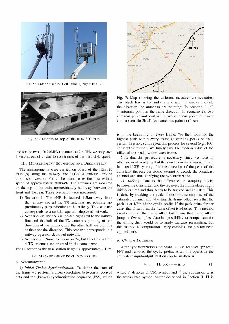
Fig. 5: Antenna setup. Left: trial 1, right: trial 2.

Fig. 6: Antennas on top of the IRIS 320 train.

and for the two (10+20MHz) channels at 2.6 GHz we only save1 second out of 2, due to constraints of the hard disk speed.

III. MEASUREMENT SCENARIOS AND DESCRIPTION

The measurements were carried on board of the IRIS320train [9] along the railway line “LGV Atlantique” around70km southwest of Paris. The train passes the area with aspeed of approximately 300km/h. The antennas are mountedon the top of the train, approximately half way between thefront and the rear. Three scenarios were measured:

1) Scenario 1: The eNB is located 1.5km away fromthe railway and all the TX antennas are pointing ap-proximately perpendicular to the railway. This scenariocorresponds to a cellular operator deployed network.

2) Scenario 2a: The eNB is located right next to the railwayline and the half of the TX antennas pointing at onedirection of the railway, and the other half are pointingat the opposite direction. This scenario corresponds to arailway operator deployed network.

3) Scenario 2b: Same as Scenario 2a, but this time all the4 TX antennas are oriented in the same sense.

For all scenarios the base station height is approximately 12m.

IV. MEASUREMENT POST PROCESSING

A. Synchronization

1) Initial Timing Synchronization: To define the start ofthe frame we perform a cross correlation between a receiveddata and the (known) synchronization sequence (PSS) which

Fig. 7: Map showing the different measurement scenarios.The black line is the railway line and the arrows indicatethe direction the antennas are pointing. In scenario 1, all4 antennas point in the same direction. In scenario 2a, twoantennas point northeast while two antennas point southwestand in scenario 2b all four antennas point northeast.

is in the beginning of every frame. We then look for thehighest peak within every frame (discarding peaks below acertain threshold) and repeat this process for several (e.g., 100)consecutive frames. We finally take the median value of theoffset of the peaks within each frame.

Note that this procedure is necessary, since we have noother mean of verifying that the synchronization was achieved.In a real LTE system, after the detection of the peak of thecorrelator the receiver would attempt to decode the broadcastchannel and thus verifying the synchronization.

2) Tracking: Due to the differences in sampling clocksbetween the transmitter and the receiver, the frame offset mightdrift over time and thus needs to be tracked and adjusted. Thisis done by tracking the peak of the impulse response of theestimated channel and adjusting the frame offset such that thepeak is at 1/8th of the cyclic prefix. If the peak drifts furtheraway than 5 samples, the frame offset is adjusted. This methodavoids jitter of the frame offset but means that frame offsetjumps a few samples. Another possibility to compensate forthe timing drift would be to apply Lanczos resampling, butthis method is computational very complex and has not beenapplied here.

B. Channel Estimation

After synchronization a standard OFDM receiver applies aFFT and removes the cyclic prefix. After this operation theequivalent input-output relation can be written as

yi′,l′ = Hi′,l′xi′,l′ + ni′,l′ , (1)

where i′ denotes OFDM symbol and l′ the subcarrier, x isthe transmitted symbol vector described in Section II, H is

the frequency domain MIMO channel matrix (MIMO transferfunction) and y is the received symbol vector.

Since the transmitted symbols are all QPSK, we can esti-mate the channel matrix as

Hi′,l′ = yi′,l′xHi′,l′ . (2)

Note that due to the orthogonal structure of the transmittedpilots in x (cf. Figure 2), Hi′,l′ will be sparse. For the easeof notation and processing we thus define new indices i =0, . . . , Ns − 1 and l = 0, . . . , Nc − 1 that refer to a block offour subcarriers and two OFDM symbols respectively (theseblocks are also highlighted in Figure 2). Thus Hi,l does notcontain any zero elements, Ns = 60, and Nc = 75, 150, 300depending on the bandwith of the carrier.

For further reference we also compute the MIMO channelimpulse response

hi,k = FFTl{Hi,l}. (3)

C. Delay-Doppler Power Spectrum Estimation

We estimate the Delay-Doppler Power Spectrum (some-times also called the scattering function) by taking the inverseFourier transform of blocks of 100 frames

St,u,k =

∣∣∣∣∣∣ 1√100Ns

100(t+1)Ns−1∑i=100tNs

hi,ke2πjiu100Ns

∣∣∣∣∣∣2

, (4)

where we have introduced the new time variable t whoseresolution depends on the carrier. In the case of the 5MHzcarrier (at 800MHz), it is 100 frames (1s) and in the case ofthe 10+20MHz carrier at 2.6GHz it is 200 frames (2s), sincewe only store the signal for one out of 2 seconds. This methodwill give us a resolution in Doppler frequency u of 1 Hz.

For the presentation in this paper, we will also compute theaverage Delay-Doppler Power profile by averaging over allelements in the MIMO matrix,

St,u,k =1

NTNR

NT−1∑m=0

NR−1∑n=0

[St,u,k]m,n, (5)

Last but not least we will also make use of the marginalDoppler profile by integrating over the delay time k

Dt,u =

Nc−1∑k=0

St,u,k, (6)

V. CHANNEL CHARACTERIZATION RESULTS

A. Path Loss

We estimate the path loss component as the slope (orgradient) of linear interpolation of the received signal strengthin respect to the 10 log (d):

PRX = PTX − α10 log (d) +N (7)

As an example we plot the results from trial 2, run 1 in Figure8. The average estimated path loss component for the 800MHzband is 3.2 and for 2.6GHz is 3.5, which is in line withestablished path loss models for rural areas.

10−2

10−1

100

101

102

−110

−100

−90

−80

−70

−60

−50

−40Run 1

distance [km]

RS

SI [d

Bm

]

UHF

UHF linear fit

2.6GHz

2.6GHz linear fit

Fig. 8: Path loss component

B. Delay and Doppler Spectra

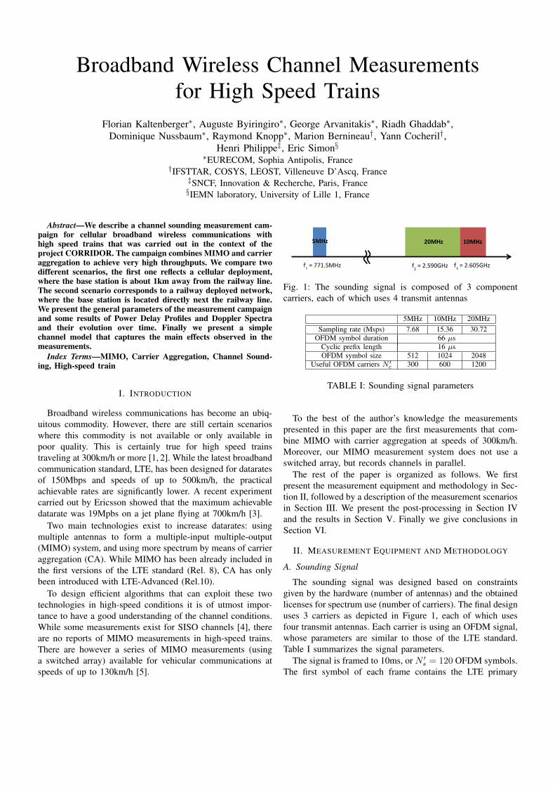
We first show the results for the 800MHz band. In Figure9 we show the Delay-Doppler Power Spectrum St,u,k of trial1, run 1 for three different blocks. At t = 50 the train isapproaching the base station, at t = 90 it is the closest tothe base station and at t = 130 it is departing from the basestation. It can be seen that there is one dominant component inthe spectrum corresponding to the line of sight (LOS), which ismoving from approximately f1 = −625Hz to f2 = −1040Hz.This effect can be seen even better in Figure 11a, where weplot the marginal Doppler Profile Dt,u over the whole run. Thedifference between these two frequencies correspond more orless exactly to Doppler bandwidth BD = 2fc

vmax

c ≈ f2 − f1.The common offset fo = f1+f2

2 correspond to the frequencyoffset in the system, which was (unfortunately) not calibratedbeforehand in the first trial.

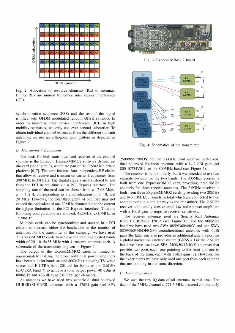
For the 2.6GHz band we show the Delay-Doppler PowerSpectrum St,u,k of trial 2, run 1, carrier A (10MHz) in Figure10 for three different blocks (approaching, close, departing).Moreover, we plot the temporal evolution of the marginalDoppler profile in Figure 11b. It can be seen that the Dopplercomponent at f1 = 1040Hz persists after the train passes thebase station (i.e., southwest of the base station) in addition tothe second Doppler component appearing at f2 = −370Hz.

This phenomenon can be also observed in run 2, where thetrain takes the same route in the other direction. As can beseen in Figure 11c, the two Doppler components are presentwhen the train approaches the base station (i.e., southwest ofthe base station) and vanish when the train has passed the basestation. Moreover this phenomenon can be observed on bothcarriers at 2.6GHz (not shown).

The results can be explained with the geometry of thescattering environment and the antenna patterns as depictedin Figure 12. The near scatterers to the left and the rightof the railway line are the poles of the gantries that supportthe railway electrification system. They are about 30m apartand act as reflectors. Some of the reflected rays arrive at thereceiver on the train at an angle almost opposite to the LOScomponent and thus have the opposite Doppler shift.

Fig. 9: Doppler Delay Power Spectrum for the 800MHz band, trial 1, run 1

Fig. 10: Doppler Delay Power Spectrum for the 2.6GHz band, trial 2, run 1

(a) 800MHz band, trial 1, run 1 (b) 2.6GHz band, trial 2, run 1 (c) 2.6GHz band, trial 2, run 2

Fig. 11: Temporal evolution of Doppler profiles for selected trials, bands, and runs.

The difference in the lengths of the LOS path and the firstreflected path is smaller than the temporal resolution of themeasurement and thus both rays appear to have the same delay.There are however also some reflections coming from gantriesfurther away and thus show a higher delay in the Doppler-delay power spectrum. Moreover, also some far scatterers canbe seen in the results, which might be coming from houses ortowers further away.

The reason why these reflections can only be seen whenthe train is southwest of the base station can be explainedusing the antenna patterns. As indicated in Section II-B, wehave only used one antenna port of the bidirectional antennas,namely the ones that point towards the front of the train (when

heading southwest). This antenna pattern is also indicated inFigure 12. The gain difference between rays arriving from thefront and arrays arriving from the back is more than 10 dB[8]. Since the reflected and the LOS ray seem to have thesame power when the train is southwest of the base station, itmeans that their difference is actually about 10dB. Now whenthe train is northeast of the base station the main lobe of theantenna is pointing at the base station and the reflected rayshave a 20 dB attenuation w.r.t. the LOS path. Therefore theyare much less visible on the Doppler-delay power profile.

The reflections from the near scatterers are also visible inthe 800MHz band, but again much less pronounced due to thefact that the antenna used is omnidirectional.

RX

TX

LOS Near scatterers

v

Far scatterer

Fig. 12: Model of the scattering environment. The antennapattern shown corresponds to one of the antenna ports of the2.6GHz antenna.

C. Power on the null-subcarriers

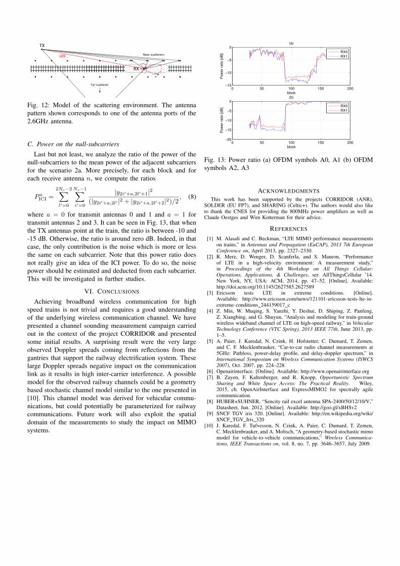
Last but not least, we analyze the ratio of the power of thenull-subcarriers to the mean power of the adjacent subcarriersfor the scenario 2a. More precisely, for each block and foreach receive antenna n, we compute the ratios

P aICI =

2Nc−2∑l′=0

Ns−1∑i′=0

|y2i′+a,2l′+1|2

(|y2i′+a,2l′ |2 + |y2i′+a,2l′+2|2)/2, (8)

where a = 0 for transmit antennas 0 and 1 and a = 1 fortransmit antennas 2 and 3. It can be seen in Fig. 13, that whenthe TX antennas point at the train, the ratio is between -10 and-15 dB. Otherwise, the ratio is around zero dB. Indeed, in thatcase, the only contribution is the noise which is more or lessthe same on each subcarrier. Note that this power ratio doesnot really give an idea of the ICI power. To do so, the noisepower should be estimated and deducted from each subcarrier.This will be investigated in further studies.

VI. CONCLUSIONS

Achieving broadband wireless communication for highspeed trains is not trivial and requires a good understandingof the underlying wireless communication channel. We havepresented a channel sounding measurement campaign carriedout in the context of the project CORRIDOR and presentedsome initial results. A surprising result were the very largeobserved Doppler spreads coming from reflections from thegantries that support the railway electrification system. Theselarge Doppler spreads negative impact on the communicationlink as it results in high inter-carrier interference. A possiblemodel for the observed railway channels could be a geometrybased stochastic channel model similar to the one presented in[10]. This channel model was derived for vehicular commu-nications, but could potentially be parameterized for railwaycommunications. Future work will also exploit the spatialdomain of the measurements to study the impact on MIMOsystems.

0 50 100 150 200−15

−10

−5

0(a)

Po

we

r ra

tio

[d

B]

block

RX0

RX1

0 50 100 150 200−20

−15

−10

−5

0(b)

block

Po

we

r ra

tio

[d

B]

RX0

RX1

Fig. 13: Power ratio (a) OFDM symbols A0, A1 (b) OFDMsymbols A2, A3

ACKNOWLEDGMENTS

This work has been supported by the projects CORRIDOR (ANR),SOLDER (EU FP7), and SHARING (Celtic+). The authors would also liketo thank the CNES for providing the 800MHz power amplifiers as well asClaude Oestges and Wim Kotterman for their advice.

REFERENCES

[1] M. Alasali and C. Beckman, “LTE MIMO performance measurementson trains,” in Antennas and Propagation (EuCAP), 2013 7th EuropeanConference on, April 2013, pp. 2327–2330.

[2] R. Merz, D. Wenger, D. Scanferla, and S. Mauron, “Performanceof LTE in a high-velocity environment: A measurement study,”in Proceedings of the 4th Workshop on All Things Cellular:Operations, Applications, & Challenges, ser. AllThingsCellular ’14.New York, NY, USA: ACM, 2014, pp. 47–52. [Online]. Available:http://doi.acm.org/10.1145/2627585.2627589

[3] Ericsson tests LTE in extreme conditions. [Online].Available: http://www.ericsson.com/news/121101-ericsson-tests-lte-in-extreme-conditions 244159017 c

[4] Z. Min, W. Muqing, S. Yanzhi, Y. Deshui, D. Shiping, Z. Panfeng,Z. Xiangbing, and G. Shuyun, “Analysis and modeling for train-groundwireless wideband channel of LTE on high-speed railway,” in VehicularTechnology Conference (VTC Spring), 2013 IEEE 77th, June 2013, pp.1–5.

[5] A. Paier, J. Karedal, N. Czink, H. Hofstetter, C. Dumard, T. Zemen,and C. F. Mecklenbrauker, “Car-to-car radio channel measurements at5GHz: Pathloss, power-delay profile, and delay-doppler spectrum,” inInternational Symposium on Wireless Communication Systems (ISWCS2007), Oct. 2007, pp. 224–228.

[6] Openairinterface. [Online]. Available: http://www.openairinterface.org[7] B. Zayen, F. Kaltenberger, and R. Knopp, Opportunistic Spectrum

Sharing and White Space Access: The Practical Reality. Wiley,2015, ch. OpenAirInterface and ExpressMIMO2 for spectrally agilecommunication.

[8] HUBER+SUHNER, “Sencity rail excel antenna SPA-2400/50/12/10/V,”Datasheet, Jun. 2012. [Online]. Available: http://goo.gl/xBHSv2

[9] SNCF TGV iris 320. [Online]. Available: http://en.wikipedia.org/wiki/SNCF TGV Iris 320

[10] J. Karedal, F. Tufvesson, N. Czink, A. Paier, C. Dumard, T. Zemen,C. Mecklenbrauker, and A. Molisch, “A geometry-based stochastic mimomodel for vehicle-to-vehicle communications,” Wireless Communica-tions, IEEE Transactions on, vol. 8, no. 7, pp. 3646–3657, July 2009.