British Columbia Institute of Technology Calculus for Business and
69
British Columbia Institute of Technology Calculus for Business and Economics Lecture Notes Kevin Wainwright PhD August 17, 2012 Contents 1 Matrix Algebra 4 1.1 Matrices and Vectors ......................... 4 1.2 Vectors as special matrices ...................... 5 1.2.1 Matrix Operators ....................... 5 1.2.2 National Income Model ................... 8 1.2.3 Division in Matrix Algebra ................. 8 1.3 Linear Dependance .......................... 9 1.4 Commutative, Associative, and Distributive Laws ......... 10 1.4.1 Communicative Law of Addition .............. 10 1.4.2 Similarly Associative Law of Addition ........... 11 1.4.3 Matrix Multiplication .................... 11 1.4.4 Associative Law ....................... 11 1.4.5 Distributive Law ....................... 12 1.5 Identity Matrices and Null Matrices ................ 12 1.5.1 Identity matrix: ........................ 12 1.5.2 Null Matrices ......................... 13 1.6 Idiosyncracies of matrix algebra ................... 13 1.7 Transposes and Inverses ....................... 13 2 Linear Dependence and Determinants 15 2.1 Using Laplace expansion ....................... 17 2.2 Cofactors ............................... 18 2.3 Rank of a Matrix ........................... 19 3 Matrix Inversion 19 4 CramersRule 20 4.1 Example: The Market Model .................... 21 4.2 Example: National Income Model .................. 22 1
Transcript of British Columbia Institute of Technology Calculus for Business and

British Columbia Institute of TechnologyCalculus for Business and Economics
Lecture Notes
Kevin Wainwright PhD
August 17, 2012
Contents
1 Matrix Algebra 41.1 Matrices and Vectors . . . . . . . . . . . . . . . . . . . . . . . . . 41.2 Vectors as special matrices . . . . . . . . . . . . . . . . . . . . . . 5
1.2.1 Matrix Operators . . . . . . . . . . . . . . . . . . . . . . . 51.2.2 National Income Model . . . . . . . . . . . . . . . . . . . 81.2.3 Division in Matrix Algebra . . . . . . . . . . . . . . . . . 8
1.3 Linear Dependance . . . . . . . . . . . . . . . . . . . . . . . . . . 91.4 Commutative, Associative, and Distributive Laws . . . . . . . . . 10
1.4.1 Communicative Law of Addition . . . . . . . . . . . . . . 101.4.2 Similarly Associative Law of Addition . . . . . . . . . . . 111.4.3 Matrix Multiplication . . . . . . . . . . . . . . . . . . . . 111.4.4 Associative Law . . . . . . . . . . . . . . . . . . . . . . . 111.4.5 Distributive Law . . . . . . . . . . . . . . . . . . . . . . . 12
1.5 Identity Matrices and Null Matrices . . . . . . . . . . . . . . . . 121.5.1 Identity matrix: . . . . . . . . . . . . . . . . . . . . . . . . 121.5.2 Null Matrices . . . . . . . . . . . . . . . . . . . . . . . . . 13
1.6 Idiosyncracies of matrix algebra . . . . . . . . . . . . . . . . . . . 131.7 Transposes and Inverses . . . . . . . . . . . . . . . . . . . . . . . 13
2 Linear Dependence and Determinants 152.1 Using Laplace expansion . . . . . . . . . . . . . . . . . . . . . . . 172.2 Cofactors . . . . . . . . . . . . . . . . . . . . . . . . . . . . . . . 182.3 Rank of a Matrix . . . . . . . . . . . . . . . . . . . . . . . . . . . 19
3 Matrix Inversion 19
4 Cramer’s Rule 204.1 Example: The Market Model . . . . . . . . . . . . . . . . . . . . 214.2 Example: National Income Model . . . . . . . . . . . . . . . . . . 22
1

5 Derivatives: The Five Basic Rules 225.1 Nonlinear Functions . . . . . . . . . . . . . . . . . . . . . . . . . 225.2 The Derivative . . . . . . . . . . . . . . . . . . . . . . . . . . . . 235.3 The Five Rules . . . . . . . . . . . . . . . . . . . . . . . . . . . . 24
5.3.1 The Constant Rule . . . . . . . . . . . . . . . . . . . . . . 245.3.2 Power Function Rule . . . . . . . . . . . . . . . . . . . . . 245.3.3 Sum-difference Rule . . . . . . . . . . . . . . . . . . . . . 255.3.4 Product Rule . . . . . . . . . . . . . . . . . . . . . . . . . 255.3.5 Quotient Rule . . . . . . . . . . . . . . . . . . . . . . . . . 26
6 The Chain Rule 266.1 The Rule: . . . . . . . . . . . . . . . . . . . . . . . . . . . . . . . 266.2 Some Examples . . . . . . . . . . . . . . . . . . . . . . . . . . . . 276.3 Combining the Chain Rule with Product and Quotient Rule . . . 27
7 Natural Logarithm and the Exponential e 297.1 Differentials . . . . . . . . . . . . . . . . . . . . . . . . . . . . . . 31
8 Implicit Differentiation 318.1 The difference between dy and ∆y . . . . . . . . . . . . . . . . . 37
9 Partial Derivatives 389.1 Two Variable Case: . . . . . . . . . . . . . . . . . . . . . . . . . . 38
9.2 Rules of Partial Differentiation . . . . . . . . . . . . . . . . . . . 399.3 Further Examples: . . . . . . . . . . . . . . . . . . . . . . . . . . 39
9.4 A Special Function: Cobb-Douglas . . . . . . . . . . . . . . . . . 419.5 Differentials . . . . . . . . . . . . . . . . . . . . . . . . . . . . . . 419.6 The two variable case . . . . . . . . . . . . . . . . . . . . . . . . 42
10 The Implicit Function Theorem 43
11 Using Calculus For Maximization Problems 4511.1 One Variable Case . . . . . . . . . . . . . . . . . . . . . . . . . . 4511.2 Two Variable Case . . . . . . . . . . . . . . . . . . . . . . . . . . 45
11.2.1 Second order Conditions (second derivative Test) . . . . . 4611.3 Rules for two variable Maximums and Minimums . . . . . . . . . 4711.4 Hessian Matrix of Second Partials: . . . . . . . . . . . . . . . . . 4711.5 Example: Two Market Monopoly with Joint Costs . . . . . . . . 4711.6 Example: Profit Max Capital and Labour . . . . . . . . . . . . . 4911.7 Example: Cobb-Douglas production function and a competitive
firm . . . . . . . . . . . . . . . . . . . . . . . . . . . . . . . . . . 5011.8 Cournot Doupoly (Game Theory) . . . . . . . . . . . . . . . . . . 5111.9 Review of Some Derivative Rules . . . . . . . . . . . . . . . . . . 5211.10Finding the MRS from Utility functions . . . . . . . . . . . . . . 53
2

12 The Lagrange Multiplier Method 5512.0.1 Example 1: max xy subject to linear constraint . . . . . . 5512.0.2 Example 2: Utility Maximization . . . . . . . . . . . . . . 5612.0.3 Example 3: Cost minimization . . . . . . . . . . . . . . . 56
12.1 Duality of the consumer choice problem . . . . . . . . . . . . . . 5712.1.1 Example 4: Utility Maximization . . . . . . . . . . . . . . 5712.1.2 Example 5: Minimization Problem . . . . . . . . . . . . . 57
12.2 Application: Intertemporal Utility Maximization . . . . . . . . . 5812.2.1 Method One:Find MRS and Substitute . . . . . . . . . . 58
12.2.2 Method Two: Use the Lagrange Multiplier Method . . . . 5912.3 Problems: . . . . . . . . . . . . . . . . . . . . . . . . . . . . . . 60
13 Kuhn-Tucker: Lagrange with Inequality Constraints 6113.1 Utility Maximization with a simple rationing constraint . . . . . 61
13.1.1 Procedure: . . . . . . . . . . . . . . . . . . . . . . . . . . 61
13.1.2 Solving by Trial and Error . . . . . . . . . . . . . . . . . . 63
13.2 War-Time Rationing . . . . . . . . . . . . . . . . . . . . . . . . . 6413.3 Peak Load Pricing . . . . . . . . . . . . . . . . . . . . . . . . . . 6613.4 Problems . . . . . . . . . . . . . . . . . . . . . . . . . . . . . . . 69
3

1 Matrix Algebra
1. Gives us a shorthand way of writing a large system of equations.
2. Allows us to test for the existance of solutions to simultaneous systems.
3. Allows us to solve a simultaneous system.
DRAWBACK: Only works for linear systems. However, we can often covertnon-linear to linear systems.Example
y = axb
ln y = ln a+ b lnx
1.1 Matrices and Vectors
Giveny = 10− x ⇒ x+ y = 10y = 2 + 3x ⇒ −3x+ y = 2
In matrix formM a t r ix o f
C o e ffi c i e n t s[1 1−3 1
] Ve c t o r o f
U n k n ow n s[xy
]=
Ve c t o r o f
C o n s t a n t s[102
]In general
a11x1 + a12x2 + . . .+ a1nxn = d1
a21x1 + a22x2 + . . .+ a2nxn = d2
..............................am1x1 + am2x2 + . . .+ amnxn = dm
n-unknowns (x1,x2, . . . xn)
Matrix forma11 a12 . . . a1n
a21 a22 . . . a2n
... . . .. . .
...am1 am2 . . . amn
x1
x2
...xn
=
d1
d2
...dm
Matrix shorthand
Ax = d
Where:A= coeffi cient martrix or an arrayx= vector of unknowns or an arrayd= vector of constants or an array
4

Subscript notationaij
is the coeffi cient found in the i-th row (i=1,. . . ,m) and the j-th column(j=1,. . . ,n)
1.2 Vectors as special matrices
The number of rows and the number of columns define the DIMENSION of amatrix.A is m rows and n is columns or ”mxn.”A matrix containing 1 column is called a ”column VECTOR”
x is a n×1 column vectord is a m×1 column vector
If x were arranged in a horizontal array we would have a row vector.Row vectors are denoted by a prime
x′ = [x1, x2, . . . , xn]
A 1×1 vector is known as a scalar.
x = [4] is a scalar
1.2.1 Matrix Operators
If we have two matrices, A and B, then
A = B iff aij = bij
Addition and Subtraction of Matrices Suppose A is an m×n matrix andB is a p×q matrix then A and B is possible only if m=p and n=q. Matricesmust have the same dimensions.[
a11 a12
a21 a22
]+
[b11 b12
b21 b22
]=
[(a11 + b11) (a12 + b12)(a21 + b21) (a22 + b22)
]=
[c11 c12
c21 c22
]Subtraction is identical to addition[
9 43 1
]−[
7 21 6
]=
[(9− 7) (4− 2)(3− 1) (1− 6)
]=
[2 22 −5
]
5

Scalar Multiplication Suppose we want to multiply a matrix by a scalar
k × A1× 1 m× n
We multiply every element in A by the scalar k
kA =
ka11 ka12 . . . ka1n
ka21 ka22 . . . ka2n
...kam1 kam2 . . . kamn
Example
Let k=[3] and A=[
6 24 5
]then kA=
kA =
[3× 6 3× 23× 4 3× 5
]=
[18 612 15
]Multiplication of Matrices To multiply two matrices, A and B, together itmust be true that for
A × B = Cm× n n× q m× q
That A must have the same number of columns (n) as B has rows (n).The product matrix, C, will have the same number of rows as A and the
same number of columns as B.
ExampleA × B = C
(1× 3) (3× 4) (1× 4)1row 3rows 1row3cols 4cols 4cols
In general
A × B × C × D = E(3× 2) (2× 5) (5× 4) (4× 1) (3× 1)
To multiply two matrices:(1) Multiply each element in a given row by each element in a given column(2) Sum up their products
Example 1 [a11 a12
a21 a22
]×[b11 b12
b21 b22
]=
[c11 c12
c21 c22
]
6
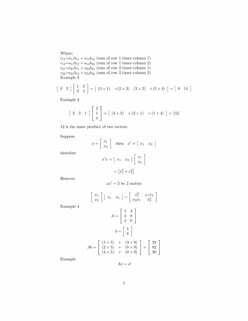
Where:c11=a11b11 + a12b21 (sum of row 1 times column 1)c12=a11b12 + a12b22 (sum of row 1 times column 2)c21=a21b11 + a22b21 (sum of row 2 times column 1)c22=a21b12 + a22b22 (sum of row 2 times column 2)Example 2
[3 2
] [ 1 23 4
]=[
(3× 1) +(2× 3) (3× 2) +(2× 4)]
=[
9 14]
Example 3
[3 2 1
] 214
=[
(3× 2) + (2× 1) + (1× 4)]
= [12]
12 is the inner product of two vectors.
Suppose
x =
[x1
x2
]then x′ =
[x1 x2
]therefore
x′x =[x1 x2
] [ x1
x2
]=[x2
1 + x22
]However
xx′ = 2 by 2 matrix
[x1
x2
] [x1 x2
]=
[x2
1 x1x2
x2x1 x22
]Example 4
A =
1 32 84 0
b =
[59
]
Ab =
(1× 5) + (3× 9)(2× 5) + (8× 9)(4× 5) + (0× 9)
=
328220
Example
Ax = d
7
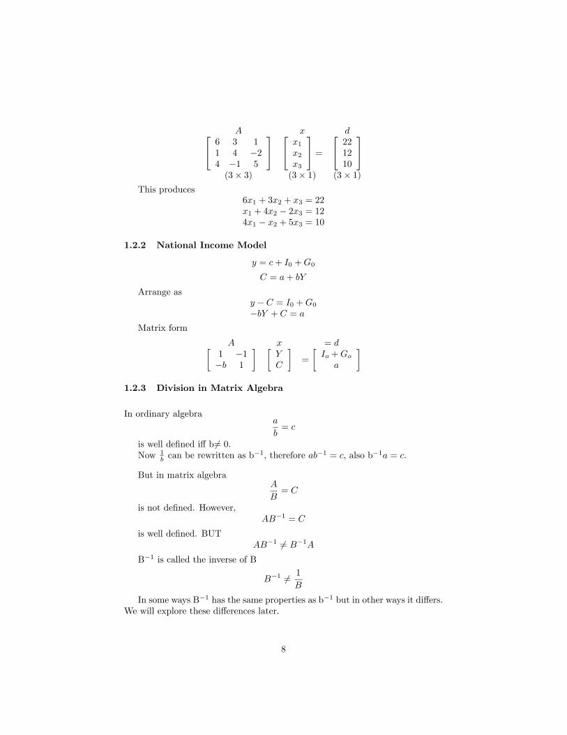
A x d 6 3 11 4 −24 −1 5
x1
x2
x3
=
221210
(3× 3) (3× 1) (3× 1)
This produces6x1 + 3x2 + x3 = 22x1 + 4x2 − 2x3 = 124x1 − x2 + 5x3 = 10
1.2.2 National Income Model
y = c+ I0 +G0
C = a+ bY
Arrange asy − C = I0 +G0
−bY + C = a
Matrix form
A x = d[1 −1−b 1
] [YC
]=
[Io +Go
a
]1.2.3 Division in Matrix Algebra
In ordinary algebraa
b= c
is well defined iff b6= 0.Now 1
b can be rewritten as b−1, therefore ab−1 = c, also b−1a = c.
But in matrix algebraA
B= C
is not defined. However,AB−1 = C
is well defined. BUTAB−1 6= B−1A
B−1 is called the inverse of B
B−1 6= 1
B
In some ways B−1 has the same properties as b−1 but in other ways it differs.We will explore these differences later.
8

1.3 Linear Dependance
Suppose we have two equations
x1 + 2x2 = 13x1 + 6x2 = 3
To solve3 [−2x2 + 1]− 6x2 = 36x2 + 3− 6x2 = 33 = 3
There is no solution. These two equations are linearly dependent. Equation2 is equal to two times equation one.[
1 23 6
] [x1
x2
]=
[13
]Ax = d
where A is a two column vectors U1
13
U2
26
Or A is two row vector
V ′1 = [1 2]
V ′2 = [3 6]
Where column two is twice column one and/or row two is three times rowone
2U1 = U2 or 3V ′1 = V ′2
Linear Dependence Generally:A set of vectors is said to be linearly dependent iff any one of them can be
expressed as a linear combination of the remaining vectors.
Example:Three vectors,
V1 =
[27
]V2 =
[18
]V3 =
[45
]are linearly dependent since
3V1 − 2V2 = V3[621
]−[
216
]=
[45
]
9

or expressed as3V1 − 2V2 − V3 = 0
General RuleA set of vectors, V1,V2,...,Vn are linearly dependent if there exsists a set of
scalars (i=1,. . . ,n). Not all equal to zero, such that
n∑i=1
= kiVi = 0
Noten∑i=1
kiVi = k1V1 + k2V2 + . . .+ knVn
1.4 Commutative, Associative, and Distributive Laws
From Highschool algebra we know commutative law of addition,
a+ b = b+ a
commutative law of multiplication,
ab = ba
Associative law of addition,
(a+ b) + c = a+ (b+ c)
associative law of multiplication,
(ab)c = a(bc)
Distributive lawa(b+ c) = ab+ ac
In matrix algebra most, but not all, of these laws are true.
1.4.1 Communicative Law of Addition
A+B = B +A
Since we are adding individual elements and aij + bij = bij +aij for all i andj.
10

1.4.2 Similarly Associative Law of Addition
A+ (B + C) = (A+B) + C
for the same reasons.
1.4.3 Matrix Multiplication
Matrix multiplication in not communtative
AB 6= BA
Example 1Let A be 2×3 and B be 3×2
A × B = C whereas B × A = C(2× 3) (3× 2) (2× 2) (3× 2) (2× 3) (3× 3)
Example 2
Let A=[
1 23 4
]and B=
[0 −16 7
]
AB =
[(1× 10) + (2× 6) (1×−1) + (2× 7)(3× 0) + (4× 6) (3×−1) + (4× 7)
]=
[12 1324 25
]But
BA =
[(0)(1)− (1)(3) (0)(2)− (1)(4)(6)(1) + (7)(3) (6)(2) + (7)(4)
]=
[−3 −427 40
]Therefore, we realize the distinction of post multiply and pre multiply. In
the caseAB = C
B is pre multiplied by A, A is post multiplied by B.
1.4.4 Associative Law
Matrix multiplication is associative
(AB)C = A(BC) = ABC
as long as their dimensions conform to our earlier rules of multiplication.
A × B × C(m× n) (n× p) (p× q)
11

1.4.5 Distributive Law
Matrix multiplication is distributive
A(B + C) = AB +AC Pre multiplication(B + C)A = BA+ CA Post multiplication
1.5 Identity Matrices and Null Matrices
1.5.1 Identity matrix:
is a square matrix with ones on its principal diagonals and zeros everywhereelse.
I2 =
[1 00 1
]I3 =
1 0 00 1 00 0 1
In =
1 0 . . . n
0 1...
.... . . 0
0 . . . 0 1
Identity Matrix in scalar algebra we know
1× a = a× 1 = a
In matrix algebra the identity matrix plays the same role
IA = AI = A
Example 1
Let A=[
1 32 4
]
IA =
[1 00 1
] [1 32 4
]=
[(1× 1) + (0× 2) (1× 3) + (0× 4)(0× 1) + (1× 2) (0× 3) + (1× 4)
]=
[1 32 4
]
Example 2
Let A=[
1 2 32 0 3
]
IA =
[1 00 1
] [1 2 32 0 3
]=
[1 2 32 0 3
]= A {I2Case}
AI =
[1 2 32 0 3
] 1 0 00 1 00 0 1
=
[1 2 32 0 3
]= A {I3Case}
Furthermore,
AIB = (AI)B = A(IB) = AB(m× n)(n× p) (m× n)(n× p)
12

1.5.2 Null Matrices
A null matrix is simply a matrix where all elements equal zero.
0 =
[0 00 0
]0 =
[0 0 00 0 0
](2× 2) (2× 3)
The rules of scalar algebra apply to matrix algebra in this case.
Examplea+ 0 = a⇒ {scalar}
A+ 0 =
[a11 a12
a21 a22
]+
[0 00 0
]= A {matrix}
A× 0 =
[a11 a12 a13
a21 a22 a23
]=
000
=
[00
]= 0
1.6 Idiosyncracies of matrix algebra
1) We know AB6=BA2)ab=0 implies a or b=0In matrix
AB =
[2 41 2
] [−2 41 −2
]=
[0 00 0
]
1.7 Transposes and Inverses
1) Transpose: is when the rows and columns are interchanged.Transpose of A = A′or AT
Example
If A=[
3 8 −91 0 4
]and B=
[3 41 7
]
A’=
3 18 0−9 4
and B’=[ 3 41 7
]Symmetrix Matrix
If A=
1 0 40 3 74 7 2
then A’= 1 0 4
0 3 74 7 2
A is a symmetric matrix.
13
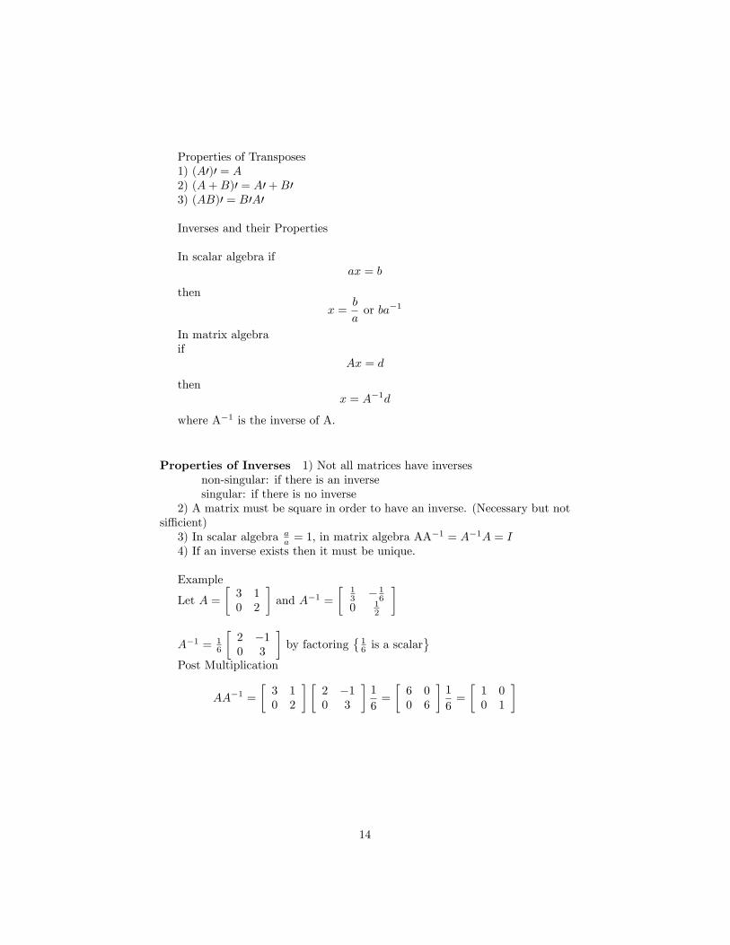
Properties of Transposes1) (A′)′ = A2) (A+B)′ = A′+B′3) (AB)′ = B′A′
Inverses and their Properties
In scalar algebra ifax = b
then
x =b
aor ba−1
In matrix algebraif
Ax = d
thenx = A−1d
where A−1 is the inverse of A.
Properties of Inverses 1) Not all matrices have inversesnon-singular: if there is an inversesingular: if there is no inverse
2) A matrix must be square in order to have an inverse. (Necessary but notsiffi cient)3) In scalar algebra a
a = 1, in matrix algebra AA−1 = A−1A = I4) If an inverse exists then it must be unique.
Example
Let A =
[3 10 2
]and A−1 =
[13 − 1
60 1
2
]
A−1 = 16
[2 −10 3
]by factoring
{16 is a scalar
}Post Multiplication
AA−1 =
[3 10 2
] [2 −10 3
]1
6=
[6 00 6
]1
6=
[1 00 1
]
14

Pre Multiplication
A−1A =1
6
[2 −10 3
] [3 10 2
]=
1
6
[6 00 6
]=
[1 00 1
]Further properties If A and B are square and non-singular then:1) (A−1)−1 = A2) (AB)−1 = B−1A−1
3) (A′)−1 = (A−1)1
Solving a linear system
SupposeA x = d
(3× 3) (3× 1) (3× 1)
thenA−1 A x = A−1 d
(3× 3) (3× 3) (3× 1) (3× 3) (3× 1)
I x = A−1 d(3× 3) (3× 1) (3× 3) (3× 1)
x = A−1d
ExampleAx = d
A =
6 3 11 4 −24 −1 5
x =
x1
x2
x3
d =
221210
A−1 =1
52
18 −16 −10−13 26 13−17 18 21
then x1
x2
x3
=1
52
18 −16 −10−13 26 13−17 18 21
221210
=
231
x∗1 = 2 x∗2 = 3 x∗3 = 1
2 Linear Dependence and Determinants
Suppose we have the following
1. x1 + 2x2 = 12. 2x1 + 4x2 = 2
15

where equation two is twice equation one. Therefore, there is no solution forx1, x2.
In matrix form:Ax = d
A[1 22 4
] x[x1
x2
]=
d[12
]The determinant of the coeffi cient matrix is
|A| = (1)(4)− (2)(2) = 0
a determinant of zero tells us that the equations are linearly dependent.Sometimes called a ”vanishing determinant.”
In general, the determinant of a square matrix, A is written as |A| or detA.
For two by two case
|A| = a11 a12
a21 a22= a11a22 − a12a21 = k
where k is uniqueany k6= 0 implies linear independence
Example 1
A=[
3 21 5
]|A| = (3× 5)− (1× 2) = 13 {Non-singular}
Example 2
B =
[2 68 24
]|B| = (2× 24)− (6× 8) = 0 {Singular}
Three by three case
Given A =
a1 a2 a3
b1 b2 b3c1 c2 c3
then
|A| = (a1b2c3) + (a2b3c1) + (b1c2a3)− (a3b2c1)− (a2b1c3)− (b3c2a1)
Cross-diagonals
16

a1 a3a2
b1 b2
c1
b3
c2 c3
Multiple along the diagonals and add up their products⇒The product along the solid lines are given a positive sign⇒The product of the dashed lines are negative.
2.1 Using Laplace expansion
⇒ The cross diagonal method does not work for matrices greater than three bythree⇒ Laplace expansion evaluates the determinant of a matrix, A, by means of
subdeterminants of A.
Subdeterminants or Minors
Given A =
a1 a2 a3
b1 b2 b3c1 c2 c3
By deleting the first row and first column, we get
|M11| =[b2 b3c2 c3
]The determinant of this matrix is the minor element a1.|Mij | ≡ is the subdeterminant from deleting the i-th row and the j-th column.
Given A=
a1 a2 a3
b1 b2 b3c1 c2 c3
17

then
M21 ≡[a12 a13
a32 a33
]M31≡
[a12 a13
a22 a23
]
2.2 Cofactors
A cofactor is a minor with a specific algebraic sign.
Cij = (−1)i+j |Mij |
thereforeC11 = (−1)2 |M11| = |M11|
C21 = (−1)3 |M21| = − |M21|The determinant by LaplaceExpanding down the first column
A =
a11 a12 a13
a21 a22 a23
a31 a32 a33
|A| = a11 |C11|+ a21 |C21|+ a31 |C31| =3∑i=1
ai1 |Ci1|
|A| = a11
∣∣∣∣ a22 a23
a32 a33
∣∣∣∣− a21
∣∣∣∣ a12 a13
a32 a33
∣∣∣∣+ a31
∣∣∣∣ a12 a13
a22 a23
∣∣∣∣Note: minus sign (−1)(1+2)
|A| = a11 [a22a33 − a23a32]− a21 [a12a33 − a13a32] + a31 [a12a23 − a13a22]
Laplace expansion can be used to expand along any row or any column.
ExampleThird row
|A| = a31
∣∣∣∣ a12 a13
a22 a23
∣∣∣∣− a32
∣∣∣∣ a11 a13
a21 a23
∣∣∣∣+ a33
∣∣∣∣ a11 a12
a21 a22
∣∣∣∣Example
A =
8 1 34 0 16 0 3
(1) Expand the first column
|A| = 8
∣∣∣∣ 0 10 3
∣∣∣∣− 4
∣∣∣∣ 1 30 3
∣∣∣∣+ 6
∣∣∣∣ 1 30 1
∣∣∣∣18

|A| = (8× 0)− (4× 3) + (6× 1) = −6
(2) Expand the second column
|A| = −1
∣∣∣∣ 4 16 3
∣∣∣∣+ 0
∣∣∣∣ 8 36 3
∣∣∣∣− 0
∣∣∣∣ 8 34 1
∣∣∣∣|A| = (−1× 6) + (0)− (0) = −6
Suggestion: Try to choose an easy row or column to expand. (i.e. the oneswith zero’s in it.)
2.3 Rank of a Matrix
DefinitionThe rank of a matrix is the maximum number linearly independent rows in
the matrix.
If A is an m×n matrix, then the rank of A is
r(A) ≤ min [m,n]
Read as: the rank of A is less than or equal to the minimum of m or n.
Using Determinants to Find the Rank(1) If A is n×m and |A|=0(2) Then delete one row and one column, and find the determinant of this
new (n-1)×(n-1) matrix.(3) Continue this process until you have a non-zero determinant.
3 Matrix Inversion
Given an n×n matrix, A, the inverse of A is
A−1 =1
|A| •AdjA
where AdjA is the adjoint matrix of A. AdjA is the transpose of matrix A’scofactor matrix. It is also the adjoint, which is an n×n matrix
Cofactor Matrix (denoted C)The cofactor matrix of A is a matrix who’s elements are the cofactors of the
elements of A
19

If A =
[a11 a12
a21 a22
]then C =
[|C11| |C12||C21| |C22|
]=
[a22 −a21
−a12 a11
]Example
Let A =
[3 21 0
]⇒ |A|=-2
Step 1: Find the cofactor matrix
C =
[|C11| |C12||C21| |C22|
]=
[0 −1−2 3
]Step 2: Transpose the cofactor matrix
CT = AdjA =
[0 −2−1 3
]Step 3: Multiply all the elements of AdjA by 1
|A| to find A−1
A−1 =1
|A| •AdjA =
(−1
2
)[0 −2−1 3
]=
[0 112 − 3
2
]Step 4: Check by AA−1 = I[
3 21 0
] [0 112 − 3
2
]=
[(3)(0) + (2)( 1
2 ) (3)(1) + (2)(− 32 )
(1)(0) + (0)( 12 ) (1)(1) + (0)(− 3
2 )
]=
[1 00 1
]
4 Cramer’s Rule
Suppose:
Equation 1 a1x1 + a2x2 = d1
Equation 2 b1x1 + b2x2 = d2
orA x = d[
a1 a2
b1 b2
] [x1
x2
]=
[d1
d2
]where
A = a1b2 − a2b1 6= 0
Solve for x1 by substitutionFrom equation 1
x2 =d1 − a1x1
a2
20
and equation 2
x2 =d2 − b1x1
b2
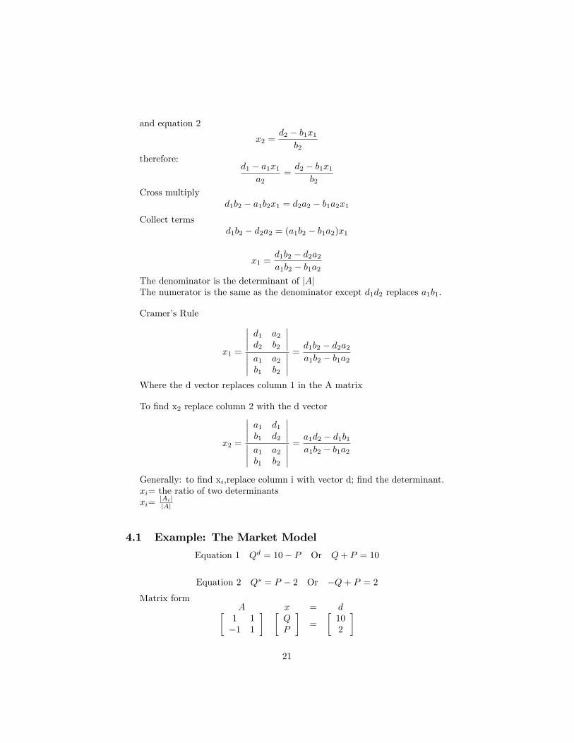
therefore:d1 − a1x1
a2=d2 − b1x1
b2
Cross multiplyd1b2 − a1b2x1 = d2a2 − b1a2x1
Collect termsd1b2 − d2a2 = (a1b2 − b1a2)x1
x1 =d1b2 − d2a2
a1b2 − b1a2
The denominator is the determinant of |A|The numerator is the same as the denominator except d1d2 replaces a1b1.
Cramer’s Rule
x1 =
∣∣∣∣ d1 a2
d2 b2
∣∣∣∣∣∣∣∣ a1 a2
b1 b2
∣∣∣∣ =d1b2 − d2a2
a1b2 − b1a2
Where the d vector replaces column 1 in the A matrix
To find x2 replace column 2 with the d vector
x2 =
∣∣∣∣ a1 d1
b1 d2
∣∣∣∣∣∣∣∣ a1 a2
b1 b2
∣∣∣∣ =a1d2 − d1b1a1b2 − b1a2
Generally: to find xi,replace column i with vector d; find the determinant.xi= the ratio of two determinantsxi=
|Ai||A|
4.1 Example: The Market Model
Equation 1 Qd = 10− P Or Q+ P = 10
Equation 2 Qs = P − 2 Or −Q+ P = 2
Matrix formA x = d[
1 1−1 1
] [QP
]=
[102
]
21

|A| = (1)(1)− (−1)(1) = 2
Find Qe
Qe =
∣∣∣∣ 10 12 1
∣∣∣∣2
=10− 2
2= 4
Find Pe
P e =
∣∣∣∣ 1 10−1 2
∣∣∣∣2
=2− (−10)
2= 6
Substitute P and Q into either equation 1 or equation 2 to verify
Qd = 10− P10− 6 = 4
4.2 Example: National Income Model
Y = C + I0 +G0 Or Y − C = I0 +G0
C = a+ bY Or −bY + c = a
In matrix form[
1 −1−b 1
] [YC
]=
[I0 +G0
a
]Solve for Ye
Y e =
∣∣∣∣ I0 +G0 −1a 1
∣∣∣∣∣∣∣∣ 1 −1−b 1
∣∣∣∣ =I0 +G0 + a
1− b
Solve for Ce
Ce =
∣∣∣∣ 1 I0 +G0
−b a
∣∣∣∣∣∣∣∣ 1 −1−b 1
∣∣∣∣ =a+ b(I0 +G0)
1− b
5 Derivatives: The Five Basic Rules
5.1 Nonlinear Functions
The term derivative means ”slope”or rate of change. The five rules we are aboutto learn allow us to find the slope of about 90% of functions used in economics,business, and social sciences.
22

y y
y
x xY = x2 Y = x1/2
xY = ax2 + bx +c
Examples ofcommon nonlinear
functions
Suppose we have a function
y = f(x) (1)
where f(x) is a non linear function. For example:
1 y = x2
2 y = 3√x = 3x1/2
3 y = ax+ bx2 + c(2)
Each equation is illustrated in Figure 1.
5.2 The Derivative
Given the general functiony = f(x)
the derivative of y is denoted as
dy
dx= f ′(x) (= y′)
23

The symbol dydx is an abbreviation for ”the change in y (dy) FROM a change inx (dx)”; or the ”rise over the run”. In other words, the slope.
5.3 The Five Rules
5.3.1 The Constant Rule
Given y = f(x) = c, where c is an arbitrary constant, then
dy
dx= f ′(x) = 0 (3)
5.3.2 Power Function Rule
Supposey = axn (4)
where a and n are any two constants. The power function rule states that theslope of the function is given by
dy
dx= f ′(x) = anxn−1 (5)
This is probably the most commonly used rule in an introductory calculuscourse. Examples
y = x2 dydx = y′ = 2x
y = 4x3 dydx = y′ = 12x2
y = 5x1/3 dydx = y′ = (5)(1/3)x1/3−1 = 5
3x−2/3
y = x dydx = y′ = (1)x1−1 = (1)x0 = 1
Some functions that do not appear to be ”power functions”can be manipulatedto take the form of equation 4. For example, if
y =1
x
then it can also be written asy = x−1
thusdy
dx= (−1)x−2
Another example,y =√x
which can also be written asy = x1/2
therefore, by equation 5,dy
dx=
1
2x−1/2
24

5.3.3 Sum-difference Rule
If y is a function created by adding or subtracting multiple functions such writtenas
y = f(x)± g(x)
where f(x) and g(x) are each functions similar to equation 4, then the derivativeof y (y′) is given by
y′ = f ′(x)± g′(x)
Example 1:y = 4x3 + 5x2
the derivative isy′ = 12x2 + 10x
Example 2:
y = x5 + 3x1/2 − 4x+ 7
y′ = 5x4 +3
2x−1/2 − 4
In each case we apply the power function rule (or constant rule) term-by-term
5.3.4 Product Rule
Suppose y is a composite function created by multiplying two functions together
y = f(x)g(x)
the derivative is given bydy
dx= f ′g + fg′ (6)
Example:y = (3x2 + 4)(x3 − 5x)
First, break this up into f(x) and g(x):
f(x) = 3x2 + 4 g(x) = x3 − 5x
then find the derivative for each
f ′(x) = 6x g′(x) = 3x2 − 5
Now re-combine the parts according to equation 6
dy
dx= f ′g + fg′ = [6x]
[x3 − 5x
]+[3x2 + 4
] [3x2 − 5
]then you simply collect terms and simplify
25

5.3.5 Quotient Rule
Suppose
y =f(x)
g(x)
thendy
dx=f ′g − fg′
[g]2(7)
Example
y =x2 + 3
2x− 1
therefore f = x2 + 3 and g = 2x− 1. The derivatives are
f ′ = 2xg′ = 2
Subsitute the componants into equation 7
dy
dx=f ′g − fg′
[g]2=
(2x) (2x− 1)−(x2 + 3
)(2)
(2x− 1)2
which (of course) can be further simplified
OPMT 5701 Lecture Notes
6 The Chain Rule
Of all the basic rules of derivatives, the most challenging one is the chain rule.However, like the other rules, if you break it down to simple steps, it too is quitemanageble. There are a couple of approaches to learning the chain rule. Bothare equally good, it just comes down to preference.The good news is that once you have mastered the chain rule —combined
with the first five —you are ready to tackle about 90% of the calculus problemsfound in business courses (including graduate programs like the MBA!)
6.1 The Rule:
Suppose y is a "nested" function of x, where nested mean "a function inside afunction".
y = f [g(x)]
where g(x) is nested inside f . then the derivative is
dy
dx= y′ = f ′ [g(x)]× g′(x) (8)
26
The process is to start with the outside function, taking the derivative of f butleaving g(x) inside unchanged. Then find g′and multiply it by f ′.For example, if
y =(x2 + 1
)3then f = ( )
3 and g = x2 + 1. From the power function rule, we know thatthe derivative of x3 is 3x2. This is true for anything cubed! So
f ′ = 3 ( )2
(and g′ = 2x)Using equation 8, we get
y′ = f ′ [g(x)]× g′(x) = 3(x2 + 1)2 · (2x)
6.2 Some Examples
1. Example: ify = (x3 + x)1/2
where f = ( )1/2
, then
y′ = f ′ [g(x)]× g′(x) =1
2
(x3 + x
)−1/2 (3x2 + 1
)2. Example: suppose
y =1√
3x+ 7
For this one, we need to re-write this to look more like a "power-function"problem. (Remember the basics:
√x = x1/2 and 1
x = x−1) therefore
y = (3x+ 7)−1/2
Here f = ( )−1/2. apply equation 8
y′ = f ′ [g(x)]× g′(x) = −1
2(3x+ 7)
−3/2(3)
6.3 Combining the Chain Rule with Product and Quo-tient Rule
The chain rule, or "function in a function" rule: if y = f(g(x)) then y′ =f ′(g(x))× g′(x)It is usually in the form like this
y =
f(x)︷ ︸︸ ︷[g(x)]
n
27

where the derivative is
y′ =dy
dx=
f ′(x)︷ ︸︸ ︷n [g(x)]
n−1 × g′(x)
Sometimes the inside function can be a bit more complex. For example
y = [h(x)j(x)]n
by breaking it down, we see that
y =
f(x)︷ ︸︸ ︷h(x) · j(x)︸ ︷︷ ︸g(x)
n
In this case the inside function, g(x) is two functions, h(x) and j(x). The stepsare the same as before except, in this case, we need to use the product rule ong(x) (g′ = h′j + hj′)
1. Example: let y be
y =[(2x+ 1)(x1/2 − 4)
]3First, Identify the individual parts:
y =
f︷ ︸︸ ︷ h
(2x+ 1)j
(x1/2 − 4)︸ ︷︷ ︸g
3
The derivative of f (power-function rule) is
f ′ = 3[(2x+ 1)(x1/2 − 4)
]2and the derivative of g (product rule) is
g′ = h′j + hj′ = (2)(x1/2 − 4) + (2x+ 1)(
12x−1/2
)(simplify) = 2x1/2 − 8 + x1/2 + 1
2x−1/2
= x1/2 + 12x−1/2 − 8
28
Now put it all together
y′ = f ′ · g′ = 3[(2x+ 1)(x1/2 − 4)
]2 (x1/2 + 1
2x−1/2 − 8
)2. Example: suppose
y =
(6x+ 1
x3
)2
Here this one is a little more complicated. The outside function (f) is
f = ( )2
but the nested function (g) is
g(x) =6x+ 1
x3
.which will require the quotient rule rule. This one should be done in partsseperately then subsitute into equation 8. First
g′ =(6)(x3)− (2x+ 1)(3x2)
(x3)2
=6x3 − 6x3 − 3x2
x6
=−3x2
x6= −3x−4
remember that f = ( )2 and f ′ = 2 ( ) , we can use equation 8
y′ = f ′ [g(x)]× g′(x) = 2
f ′︷ ︸︸ ︷(6x+ 1
x3
)·
g′︷ ︸︸ ︷(−3x−4
)7 Natural Logarithm and the Exponential e
1. The Number e
if y = ex thendy
dx= ex
if y = ef(x) thendy
dx= ef(x) · f ′(x)
2. Examples
29

1. (a)
y = e3x
dy
dx= e3x(3)
(b)
y = e7x3
dy
dx= e7x3(21x2)
(c)
y = ert
dy
dt= rert
2. Logarithm (Natural log) lnx
(a) Rules of natural log
If Theny = AB ln y = ln(AB) = lnA+ lnBy = A/B ln y = lnA− lnBy = Ab ln y = ln(Ab) = b lnA
NOTE: ln(A+B) 6= lnA+ lnB EVER!!!
(b) derivatives
IF THEN
y = lnx dydx = 1
x
y = ln (f(x)) dydx = 1
f(x) · f′(x)
(c) Examples
i.
y = ln(x2 − 2x)
dy/dx =1
(x2 − 2x)(2x− 2)
ii.
y = ln(x1/2) =1
2lnx
dy/dx =
(1
2
)(1
x
)=
1
2x
30

7.1 Differentials
Given the function
y = f(x)
the derivative is
dy
dx= f ′(x)
However, we can treat dy/dx as a fraction and factor out the dx
dy = f ′(x)dx
where dy and dx are called differentials. If dy/dx can be interpreted as ”theslope of a function”, then dy is the ”rise”and dx is the ”run”. Another way oflooking at it is as follows:
• dy = the change in y
• dx = the change in x
• f ′(x) = how the change in x causes a change in y
Example 1 ify = x2
thendy = 2xdx
Lets suppose x = 2 and dx = 0.01. What is the change in y(dy)?
dy = 2(2)(0.01) = 0.04
Therefore, at x = 2, if x is increased by 0.01 then y will increase by 0.04.
8 Implicit Differentiation
Suppose we have the following:
2y + 3x = 12
we can rewrite it as
2y = 12− 3x
y = 6− 3
2x
31

Now we have y = f(x) and we can take the derivative
dy
dx= −3
2
Lets consider an alternative. We know that y is a function of x or, y = y(x)and the derivative of y is dydx . If we return to our original equation, 2y+3x = 12,we can differentiate it IMPLICITLY in the following manner
2y + 3x = 12
2dy + 3dx = 0
(d(12)
dx= 0
)2dy
dx+ 3
dx
dx= 0
2dy
dx+ 3 = 0
(dx
dx= 1
)rearrange to get dy
dx by itself
2dy
dx= −3
dy
dx= −3
2
which is what we got before!Here is a few more examples:
1.
y2 + x2 = 36
2ydy + 2xdx = d(36)
2ydy
dx+ 2x
dx
dx= 0
(remember
d(36)
dx= 0
)2ydy
dx+ 2x = 0
dy
dx= −2x
2y= −x
y
2.
5y3 + 4x5 = 250
15y2 dy
dx+ 20x4 = 0
15y2 dy
dx+ 20x4 = 0
dy
dx= −20x4
15y2= −4x4
3y2
32

3.
y1/2 − 2x2 + 5y = 151
2y−1/2dy − 4xdx+ 5dy = 0(1
2y−1/2 + 5
)dy
dx− 4x = 0 (÷ by dx)
dy
dx=
4x(12y−1/2 + 5
)When you are using implicit differentiation, there are two things to remem-
ber:
• First: All the rules apply as before
• Second: you are ASSUMING that you can rewrite the equation in theform y = f(x)
Example: Special application of the product rule.Suppose you want to implicitly differentiate
xy = 24
what do we do here?In this case we treat x and y as seperate functions and apply the product
rule
xdy
dx+ y
dx
dx= 0
xdy
dx+ y = 0
dy
dx= −y
x
Alternatively, we could first solve for y, then take the derivative
xy = 24
y =24
x= 24x−1
dy
dx= (−1)24x−2 = −24
x2
which does not look like what we got with implicit differentiation, but, if we usea substitution trick, remembering that originally xy = 24, we will get
dy
dx= −24
x2= −xy
x2
dy
dx= −y
x
33

Lets try it again
48 = x2y3
0 = 3x2y2 dy
dx+ 2xy3 dx
dx(Product rule and power-function rule)
3x2y2 dy
dx= −2xy3
(again
dx
dx= 1
)dy
dx= − 2xy3
3x2y2= −2y
3x
34

Level CurvesIf we have a function like z = xy or u = lnx + ln y, then z and u are both
functions of x and y. IF we fix z and u to be some particular values such as
z = z and u = u
then z and u are now treated as constants and we are evaluating the functionsz = xy and u = lnx+ ln y at a particular level. In other words, we are lookingfor values of x and y that keep z or u constant. This allows us to assume thaty is an implicit function of x, i.e.
yx = z
y =z
x
using implicit differentiation, we can find the slope of the level curve
yx = z
xdy
dx+ y
dx
dx=
d(z)
dx= 0
dy
dx= −y
x
The level curve is illustrated in figure 1In figure 1 we have graphed y as a function of x and a constant, z. This
curve plots all combinations of x and y that keep z at a constant level. Commonexamples of level curves in economics are ”indifference curves”(constant utility)and ”isoquants” (constant levels of output).Lets look at the utility function example
u = lnx+ ln y
where u = u. using implicit differentiation and the rule of logarithm derivatives
d(u)
dx=
(1
x
)+
(1
y
)dy
dx= 0
dy
dx= −
1x1y
= −yx
Alternatively, we could try to first write this function such that we explicitlyhave y as a function of x. However, this would require us to ”unlog”the function,i.e.
u = lnx+ ln y
u = ln(xy)
eu = xy (unlogged)
y =eu
x
The result does not look easier to work with than when we used implicit differen-tiation. This is an example of where implicit differentiation would be preferred.
35

y zx=
y
x
dydx
1
Slope = y x
36
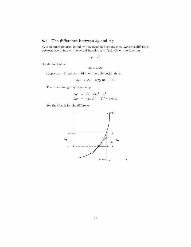
8.1 The difference between dy and ∆y
dy is an approximation found by moving along the tangency. ∆y is the differencebetween two points on the actual function y = f(x). Given the function
y = x2
the differential isdy = 2xdx
suppose x = 2 and dx = .01 then the differential, dy is
dy = 2xdx = 2(2)(.01) = .04
The other change ∆y is given by
∆y = (x+ dx)2 − x2
∆y = (2.01)2 − (2)2 = 0.0401
See the Graph for the difference
A B
C
D
dy
dx2 2.01
4
4.0401
∆y
y = x2
∆y
x
y
37

9 Partial Derivatives
Single variable calculus is really just a ”special case”of multivariable calculus.For the function y = f(x), we assumed that y was the endogenous variable, xwas the exogenous variable and everything else was a parameter. For example,given the equations
y = a+ bx
ory = axn
we automatically treated a, b, and n as constants and took the derivative of ywith respect to x (dy/dx). However, what if we decided to treat x as a constantand take the derivative with respect to one of the other variables? Nothingprecludes us from doing this. Consider the equation
y = ax
wheredy
dx= a
Now suppose we find the derivative of y with respect to a, but TREAT x as theconstant. Then
dy
da= x
Here we just ”reversed”the roles played by a and x in our equation.
9.1 Two Variable Case:
let z = f(x, y), which means ”z is a function of x and y”. In this case zis the endogenous (dependent) variable and both x and y are the exogenous(independent) variables.To measure the the effect of a change in a single independent variable (x
or y) on the dependent variable (z) we use what is known as the PARTIALDERIVATIVE.The partial derivative of z with respect to x measures the instantaneous
change in the function as x changes while HOLDING y constant. Similarly, wewould hold x constant if we wanted to evaluate the effect of a change in y on z.Formally:
• ∂z∂x is the ”partial derivative” of z with respect to x, treating y as aconstant. Sometimes written as fx.
• ∂z∂y is the ”partial derivative” of z with respect to y, treating x as aconstant. Sometimes written as fy.
38

The ”∂” symbol (”bent over” lower case D) is called the ”partial” symbol.It is interpreted in exactly the same way as dy
dx from single variable calculus.The ∂ symbol simply serves to remind us that there are other variables in theequation, but for the purposes of the current exercise, these other variables areheld constant.EXAMPLES:
z = x+ y ∂z/∂x = 1 ∂z/∂y = 1z = xy ∂z/∂x = y ∂z/∂y = xz = x2y2 ∂z/∂x = 2(y2)x ∂z/∂y = 2(x2)yz = x2y3 + 2x+ 4y ∂z/∂x = 2xy3 + 2 ∂z/∂y = 3x2y2 + 4
• REMEMBER: When you are taking a partial derivative you treat theother variables in the equation as constants!
9.2 Rules of Partial Differentiation
Product Rule: given z = g(x, y) · h(x, y)
∂z∂x = g(x, y) · ∂h∂x + h(x, y) · ∂g∂x∂z∂y = g(x, y) · ∂h∂y + h(x, y) · ∂g∂y
Quotient Rule: given z = g(x,y)h(x,y) and h(x, y) 6= 0
∂z∂x =
h(x,y)· ∂g∂x−g(x,y)· ∂h∂x[h(x,y)]2
∂z∂y =
h(x,y)· ∂g∂y−g(x,y)· ∂h∂y[h(x,y)]2
Chain Rule: given z = [g(x, y)]n
∂z∂x = n [g(x, y)]
n−1 · ∂g∂x∂z∂y = n [g(x, y)]
n−1 · ∂g∂y
9.3 Further Examples:
For the function U = U(x, y) find the the partial derivates with respect to xand yfor each of the following examples
Example 2U = −5x3 − 12xy − 6y5
Answer:∂U
∂x= Ux = 15x2 − 12y
∂U
∂y= Uy = −12x− 30y4
39

Example 3U = 7x2y3
Answer:
∂U
∂x= Ux = 14xy3
∂U
∂y= Uy = 21x2y2
Example 4U = 3x2(8x− 7y)
Answer:
∂U
∂x= Ux = 3x2(8) + (8x− 7y)(6x) = 72x2 − 42xy
∂U
∂y= Uy = 3x2(−7) + (8x− 7y)(0) = −21x2
Example 5U = (5x2 + 7y)(2x− 4y3)
Answer:
∂U
∂x= Ux = (5x2 + 7y)(2) + (2x− 4y3)(10x)
∂U
∂y= Uy = (5x2 + 7y)(−12y2) + (2x− 4y3)(7)
Example 6
U =9y3
x− yAnswer:
∂U
∂x= Ux =
(x− y)(0)− 9y3(1)
(x− y)2=−9y3
(x− y)2
∂U
∂y= Uy =
(x− y)(27y2)− 9y3(−1)
(x− y)2=
27xy2 − 18y3
(x− y)2
Example 7U = (x− 3y)3
Answer:
∂U
∂x= Ux = 3(x− 3y)2(1) = 3(x− 3y)2
∂U
∂y= Uy = 3(x− 3y)2(−3) = −9(x− 3y)2
40

9.4 A Special Function: Cobb-Douglas
The Cobb-douglas function is a mathematical function that is very popular ineconomic models. The general form is
z = xayb
and its partial derivatives are
∂z/∂x = axa−1yb and ∂z/∂y = bxayb−1
Furthermore, the absolute value of the slope of the level curve of a Cobb-douglas is given by
∂z/∂x
∂z/∂y= MRS =
a
b
y
x
9.5 Differentials
Given the function
y = f(x)
the derivative is
dy
dx= f ′(x)
However, we can treat dy/dx as a fraction and factor out the dx
dy = f ′(x)dx
where dy and dx are called differentials. If dy/dx can be interpreted as ”theslope of a function”, then dy is the ”rise”and dx is the ”run”. Another way oflooking at it is as follows:
• dy = the change in y
• dx = the change in x
• f ′(x) = how the change in x causes a change in y
Example 8 ify = x2
thendy = 2xdx
Lets suppose x = 2 and dx = 0.01. What is the change in y(dy)?
dy = 2(2)(0.01) = 0.04
Therefore, at x = 2, if x is increased by 0.01 then y will increase by 0.04.
41

9.6 The two variable case
Ifz = f(x, y)
then the change in z is
dz =∂z
∂xdx+
∂z
∂ydy or dz = fxdx+ fydy
which is read as ”the change in z (dz) is due partially to a change in x (dx)plus partially due to a change in y (dy). For example, if
z = xy
then the total differential is
dz = ydx+ xdy
and, if
z = x2y3
thendz = 2xy3dx+ 3x2y2dy
REMEMBER: When you are taking the total differential, you are justtaking all the partial derivatives and adding them up.
Example 9 Find the total differential for the following utility functions
1. U(x1, x2) = ax1 + bx2 (a, b > 0)
2. U(x1, x2) = x21 + x3
2 + x1x2
3. U(x1, x2) = xa1xb2
Answers:
1.
∂U∂x1
= U1 = a∂U∂x2
= U2 = b
dU = U1dx1 + U2dx2 = adx1 + bdx2
2.
∂U∂x1
= U1 = 2x1 + x2∂U∂x2
= U2 = 3x22 + x1
dU = U1dx1 + U2dx2 = (2x1 + x2)dx1 + (3x22 + x1)dx2
3.
∂U∂x1
= U1 = axa−11 xb2 =
axa1xb2
x1∂U∂x2
= U2 = bxa1xb−12 =
bxa1xb2
x2
dU =(axa1x
b2
x1
)dx1 +
(bxa1x
b2
x2
)dx2 =
[adx1x1
+ bdx2x2
]xa1x
b2
42

10 The Implicit Function Theorem
Suppose you have a function of the form
F (y, x1, x2) = 0
where the partial derivatives are ∂F/∂x1 = Fx1 , ∂F/∂x2 = Fx2and ∂F/∂y =Fy. This class of functions are known as implicit functions where F (y, x1, x2) =0 implicity define y = y(x1, x2). What this means is that it is possible (the-oretically) to rewrite to get y isolated and expressed as a function of x1 andx2. While it may not be possible to explicitly solve for y as a function of x, wecan still find the effect on y from a change in x1 or x2 by applying the implicitfunction theorem:
Theorem 10 If a function
F (y, x1, x2) = 0
has well defined continuous partial derivatives
∂F
∂y= Fy
∂F
∂x1= Fx1
∂F
∂x2= Fx2
and if, at the values where F is being evaluated, the condition that
∂F
∂y= Fy 6= 0
holds, then y is implicitly defined as a function of x. The partial derivatives ofy with respect to x1 and x2, are given by the ratio of the partial derivatives ofF, or
∂y
∂xi= −Fxi
Fyi = 1, 2
To apply the implicit function theorem to find the partial derivative of ywith respect to x1 (for example), first take the total differential of F
dF = Fydy + Fx1dx1 + Fx2dx2 = 0
then set all the differentials except the ones in question equal to zero (i.e. setdx2 = 0) which leaves
Fydy + Fx1dx1 = 0
orFydy = −Fx1dx1
43

dividing both sides by Fy and dx1 yields
dy
dx1= −Fx1
Fy
which is equal to ∂y∂x1
from the implicit function theorem.
Example 11 For each f(x, y) = 0, find dy/dx for each of the following:
1.y − 6x+ 7 = 0
Answer:dy
dx= −fx
fy= − (−6)
1= 6
2.3y + 12x+ 17 = 0
Answer:dy
dx= −fx
fy= − (−12)
3= 4
3.x2 + 6x− 13− y = 0
Answer:dy
dx= −fx
fy=−(2x+ 6)
−1= 2x+ 6
4.f(x, y) = 3x2 + 2xy + 4y3
Answer:dy
dx= −fx
fy= − 6x+ 2y
12y2 + 2x
5.f(x, y) = 12x5 − 2y
Answer:dy
dx= −fx
fy= −60x4
−2= 30x4
6.f(x, y) = 7x2 + 2xy2 + 9y4
Answer:dy
dx= −fx
fy= − 14x+ 2y2
36y3 + 4xy
Example 12 For f(x, y, z) use the implicit function theorem to find dy/dx anddy/dz :
44

1.f(x, y, z) = x2y3 + z2 + xyz
Answer:dydx = − fxfy = − 2xy3+yz
3x2y2+xz
dydz = − fzfy = − 2z+xy
3x2y2+xz
2.f(x, y, z) = x3z2 + y3 + 4xyz
Answer:dydx = − fxfy = − 3x2z2+4yz
3y2+4xz
dydz = − fzfy = − 2x3z+4xy
3y2+4xz
3.f(x, y, z) = 3x2y3 + xz2y2 + y3zx4 + y2z
Answer:dydx = − fxfy = − 6xy3+z2y2+4y3zx3
9x2y2+2xz2y+3y2zx4+2yz
dydz = − fzfy = − 2xzy2+y3x4+y2
9x2y2+2xz2y+3y2zx4+2yz
11 Using Calculus For Maximization Problems
11.1 One Variable Case
If we have the following function
y = 10x− x2
we have an example of a dome shaped function. To find the maximum of thedome, we simply need to find the point where the slope of the dome is zero, or
dydx = 10− 2x = 0
10 = 2xx = 5andy = 25
11.2 Two Variable Case
Suppose we want to maximize the following function
z = f(x, y) = 10x+ 10y + xy − x2 − y2
Note that there are two unknowns that must be solved for: x and y. Thisfunction is an example of a three-dimensional dome. (i.e. the roof of BC Place)
45

To solve this maximization problem we use partial derivatives. We take apartial derivative for each of the unknown choice variables and set them equalto zero
∂z∂x = fx = 10 + y − 2x = 0 The slope in the ”x”direction = 0∂z∂y = fy = 10 + x− 2y = 0 The slope in the ”y”direction = 0
This gives us a set of equations, one equation for each of the unknown vari-ables. When you have the same number of independent equations as unknowns,you can solve for each of the unknowns.rewrite each equation as
y = 2x− 10
x = 2y − 10
substitute one into the other
x = 2(2x− 10)− 10
x = 4x− 30
3x = 30
x = 10
similarly,y = 10
REMEMBER: To maximize (minimize) a function of many variablesyou use the technique of partial differentiation. This produces a set of equations,one equation for each of the unknowns. You then solve the set of equationssimulaneously to derive solutions for each of the unknowns.
11.2.1 Second order Conditions (second derivative Test)
To test for a maximum or minimum we need to check the second partial deriv-atives. Since we have two first partial derivative equations (fx,fy) and twovariable in each equation, we will get four second partials ( fxx, fyy, fxy, fyx)Using our original first order equations and taking the partial derivatives for
each of them (a second time) yields:
fx = 10 + y − 2x = 0 fy = 10 + x− 2y = 0
fxx = −2 fyy = −2fxy = 1 fyx = 1
The two partials,fxx, and fyy are the direct effects of of a small change in xand y on the respective slopes in in the x and y direction. The partials, fxy andfyx are the indirect effects, or the cross effects of one variable on the slope inthe other variable’s direction. For both Maximums and Minimums, the directeffects must outweigh the cross effects
46

11.3 Rules for two variable Maximums and Minimums
1. Maximum
fxx < 0
fyy < 0
fyyfxx − fxyfyx > 0
2. Minimum
fxx > 0
fyy > 0
fyyfxx − fxyfyx > 0
3. Otherwise, we have a Saddle Point
From our second order conditions, above,
fxx = −2 < 0 fyy = −2 < 0fxy = 1 fyx = 1
andfyyfxx − fxyfyx = (−2)(−2)− (1)(1) = 3 > 0
therefore we have a maximum.
11.4 Hessian Matrix of Second Partials:
Sometimes the Second Order Conditions are checked in matrix form, using aHession Matrix. The Hessian is written as
H =
[fxx fxyfyx fyy
]where the determinant of the Hessian is
|H| =∣∣∣∣ fxx fxyfyx fyy
∣∣∣∣ = fyyfxx − fxyfyx
which is the measure of the direct versus indirect strengths of the second partials.This is a common setup for checking maximums and minimums, but it is notnecessary to use the Hessian.
11.5 Example: Two Market Monopoly with Joint Costs
A monopolist offers two different products, each having the following marketdemand functions
q1 = 14− 14p1
q2 = 24− 12p2
47

The monopolist’s joint cost function is
C(q1, q2) = q21 + 5q1q2 + q2
2
The monopolist’s profit function can be written as
π = p1q1 + p2q2 − C(q1, q2) = p1q1 + p2q2 − q21 − 5q1q2 − q2
2
which is the function of four variables: p1, p2, q1,and q2. Using the marketdemand functions, we can eliminate p1and p2 leaving us with a two variablemaximization problem. First, rewrite the demand functions to get the inversefunctions
p1 = 56− 4q1
p2 = 48− 2q2
Substitute the inverse functions into the profit function
π = (56− 4q1)q1 + (48− 2q2)q2 − q21 − 5q1q2 − q2
2
The first order conditions for profit maximization are
∂π∂q1
= 56− 10q1 − 5q2 = 0∂π∂q2
= 48− 6q2 − 5q1 = 0
Solve the first order conditions using Cramer’s rule. First, rewrite in matrixform [
10 55 6
] [q1
q2
]=
[5648
]where |A| = 35
q∗1 =
∣∣∣∣ 56 548 6
∣∣∣∣35
= 2.75
q∗2 =
∣∣∣∣ 10 565 48
∣∣∣∣35
= 5.7
Using the inverse demand functions to find the respective prices, we get
p∗1 = 56− 4(2.75) = 45p∗2 = 48− 2(5.7) = 36.6
From the profit function, the maximum profit is
π = 213.94
Next, check the second order conditions to verify that the profit is at amaximum. The various second derivatives can be set up in a matrix called aHessian The Hessian for this problem is
H =
[π11 π12
π21 π22
]=
[−10 −5−5 −6
]
48

The suffi cient conditions are
|H1| = π11 = −10 < 0 (First Principle Minor of Hessian)|H2| = π11π22 − π12π21 = (−10)(−6)− (−5)2 = 35 > 0 (determinant)
Therefore the function is at a maximum. Further, since the signs of |H1| and|H2| are invariant to the values of q1and q2, we know that the profit function isstrictly concave.
11.6 Example: Profit Max Capital and Labour
Suppose we have the following production function
q = Outputq = f(K,L) = L
12 +K
12 L = Labour
K = Capital
Then the profit function for a competitive firm is
π = Pq − wL− rK P = Market Priceor w = Wage Rateπ = PL
12 + PK
12 − wL− rK r = Rental Rate
First order conditions
General Form1. ∂π
∂L = P2 L
−12 − w = 0 PfL − w = 0
2. ∂π∂k = P
2 K−12 − r = 0 PfK − r = 0
Solving (1) and (2), we get
L∗ = ( 2wP )−2 K∗ = ( 2r
P )−2
Second order conditions (Hessian)
πLL = PfLL = −P4 L
−32 < 0
πKK = PfKK = −P4 K
−32 < 0
πLK = πKL = PfLK = PfKL = 0
or, in matrix form
H =
∣∣∣∣ πLL πLKπKL πKK
∣∣∣∣ =
∣∣∣∣∣ −P4 L−32 0
0 −P4 K
−32
∣∣∣∣∣P[fLLfKK − (fLK)2
]=
(−P4L−32
)(−P4K−32
)− 0 > 0
Differentiate first order of conditions with respect to capital (K) and labour(L)
49

=⇒Therefore profit maximization
Example: If P = 1000, w = 20, and r = 10
1. Find the optimal K, L, and π
2. Check second order conditions
11.7 Example: Cobb-Douglas production function and acompetitive firm
Consider a competitive firm with the following profit function
π = TR− TC = PQ− wL− rK
where P is price, Q is output, L is labour and K is capital, and w and rare the input prices for L and K respectively. Since the firm operates in acompetitive market, the exogenous variables are P,w and r. There are threeendogenous variables, K, L and Q. However output, Q, is in turn a function ofK and L via the production function
Q = f(K,L)
which in this case, is the Cobb-Douglas function
Q = LaKb
where a and b are positive parameters. If we further assume decreasingreturns to scale, then a + b < 1. For simplicity, let’s consider the symmetriccase where a = b = 1
4
Q = L14K
14
Substituting Equation 3 into Equation 1 gives us
π(K,L) = PL14K
14 − wL− rK
The first order conditions are
∂π∂L = P
(14
)L−
34K
14 − w = 0
∂π∂K = P
(14
)L
14K−
34 − r = 0
This system of equations define the optimal L and K for profit maximization.But first, we need to check the second order conditions to verify that we have amaximum.
50

The Hessian for this problem is
H =
[πLL πLKπKL πKK
]=
[P (− 3
16 )L−74K
14 P
(14
)2L−
34K−
34
P(
14
)2L−
34K−
34 P
(− 3
16
)L
14K
74
]The suffi cient conditions for a maximum are that |H1| < 0 and |H| > 0.
Therefore, the second order conditions are satisfied.We can now return to the first order conditions to solve for the optimal K
and L. Rewriting the first equation in Equation 5 to isolate K
P(
14
)L−
34K
14 = w
K = ( 4wp L
34 )4
Substituting into the second equation of Equation 5
P4 L
14K−
34 =
(P4
)L
14
[(4wp L
34
)4]− 3
4
= r
= P 4(
14
)4w−3L−2 = r
Re-arranging to get L by itself gives us
L∗ = (P
4w−
34 r−
14 )2
Taking advantage of the symmetry of the model, we can quickly find theoptimal K
K∗ = (P
4r−
34w−
14 )2
L∗ and K∗ are the firm’s factor demand equations.
11.8 Cournot Doupoly (Game Theory)
.
Assumption: Each firm takes the other firms output as exogenous andchooses output to maximize its own profits.Market Demand:
P = a− bqorP = a− b(q1 + q2) (q1 + q2 = q)
Where qi is firm i’s outputi = 1, 2
Each firm faces the same cost function
TC = K + cqi
(i = 1, 2)
51

Each firm’s profit function is
πi = Pqi − cqi −K
Firm 1π1 = Pq1 − cq1 −K
π1 = (a− bq1 − bq2)q1 − cq1 −KMax π1, treating q2 as constant
∂π∂q1
= a− bq2 − 2bq1 − c = 0
2bq1 = a− c− bq2
q1 = a−c2b −
q22 ⇒ ”Best Response Function”
Best Response Function tells Firm 1 the profit maximizing q1 for any levelof q2.
For Firm 2
π2 = (a− bq1 − bq2)q2 − cq2 −KMax π2 Treating q1as constantq2 = a−c
2b −q12 Firm 2’s ”Best Response Function”
The two ”Best Response Functions”
Firm 1 q1 = a−c2b −
q22
Firm 2 q2 = a−c2b −
q12
gives us two equations and two unknowns.The solution to this system of equations is the equilibrium to the ”Cournot
Duopoly Game.”
Using Cramers Rule
1. q∗1 = a−c3b
2. q∗2 = a−c3b
Market Output q∗1 + q∗2 = 2(a−c)3b
11.9 Review of Some Derivative Rules
1. Partial Derivative Rules:
U = xy ∂U/∂x = y ∂U/∂y = xU = xayb ∂U/∂x = axa−1yb ∂U/∂y = bxayb−1
U = xay−b = xa
yb∂U/∂x = axa−1y−b ∂U/∂y = −bxay−b−1
U = ax+ by ∂U/∂x = a ∂U/∂y = bU = ax1/2 + by1/2 ∂U/∂x = a
(12
)x−1/2 ∂U/∂y = b
(12
)y−1/2
2. Logarithm (Natural log) lnx
52

(a) Rules of natural log
If Theny = AB ln y = ln(AB) = lnA+ lnBy = A/B ln y = lnA− lnBy = Ab ln y = ln(Ab) = b lnA
NOTE: ln(A+B) 6= lnA+ lnB
(b) derivatives
IF THEN
y = lnx dydx = 1
x
y = ln (f(x)) dydx = 1
f(x) · f′(x)
(c) Examples
If Theny = ln(x2 − 2x) dy/dx = 1
(x2−2x) (2x− 2)
y = ln(x1/2) = 12 lnx dy/dx =
(12
) (1x
)= 1
2x
3. The Number e
if y = ex thendy
dx= ex
if y = ef(x) thendy
dx= ef(x) · f ′(x)
(a) Examples
y = e3x dydx = e3x(3)
y = e7x3 dydx = e7x3(21x2)
y = ert dydt = rert
11.10 Finding the MRS from Utility functions
EXAMPLE: Find the total differential for the following utility functions
1. U(x1, x2) = ax1 + bx2 where (a, b > 0)
2. U(x1, x2) = x21 + x3
2 + x1x2
3. U(x1, x2) = xa1xb2 where (a, b > 0)
4. U(x1, x2) = α ln c1 + β ln c2 where (α, β > 0)
53

Answers:1. ∂U
∂x1= U1 = a ∂U
∂x2= U2 = b
anddU = U1dx1 + U2dx2 = adx1 + bdx2 = 0
If we rearrange to get dx2/dx1
dx2
dx1= −
∂U∂x1∂U∂x2
= −U1
U2= −a
b
The MRS is the Absolute value of dx2dx1:
MRS =a
b
2. ∂U∂x1
= U1 = 2x1 + x2∂U∂x2
= U2 = 3x22 + x1
and
dU = U1dx1 + U2dx2 = (2x1 + x2)dx1 + (3x22 + x1)dx2 = 0
Find dx2/dx1
dx2
dx1= −U1
U2= − (2x1 + x2)
(3x22 + x1)
The MRS is the Absolute value of dx2dx1:
MRS =(2x1 + x2)
(3x22 + x1)
iii) ∂U∂x1
= U1 = axa−11 xb2
∂U∂x2
= U2 = bxa1xb−12
anddU =
(axa−1
1 xb2)dx1 +
(bxa1x
b−12
)dx2 = 0
Rearrange to get
dx2
dx1= −U1
U2= −ax
a−11 xb2
bxa1xb−12
= −ax2
bx1
The MRS is the Absolute value of dx2dx1:
MRS =ax2
bx1
iv) ∂U∂c1
= U1 = α(
1c1
)dc1 =
(αc1
)dc1
∂U∂x2
= U2 = β(
1c2
)dc2 =
(βc2
)dc2
and
dU =
(α
c1
)dc1 +
(β
c2
)dc2 = 0
54

Rearrange to get
dc2dc1
= −U1
U2=
(αc1
)(βc2
) = −αc2βc1
The MRS is the Absolute value of dc2dc1:
MRS =αc2βc1
12 The Lagrange Multiplier Method
Sometimes we need to to maximize (minimize) a function that is subject tosome sort of constraint. For example
Maximize z = f(x, y)
subject to the constraint x+ y ≤ 100
For this kind of problem there is a technique, or trick, developed for this kindof problem known as the Lagrange Multiplier method. This method involvesadding an extra variable to the problem called the lagrange multiplier, or λ.We then set up the problem as follows:
1. Create a new equation form the original information
L = f(x, y) + λ(100− x− y)or
L = f(x, y) + λ [Zero]
2. Then follow the same steps as used in a regular maximization problem
∂L∂x = fx − λ = 0∂L∂y = fy − λ = 0
∂L∂λ = 100− x− y = 0
3. In most cases the λ will drop out with substitution. Solving these 3equations will give you the constrained maximum solution
12.0.1 Example 1: max xy subject to linear constraint
Suppose z = f(x, y) = xy. and the constraint is the one from above. Theproblem then becomes
L = xy + λ(100− x− y)
Now take partial derivatives, one for each unknown, including λ
55

∂L∂x = y − λ = 0∂L∂y = x− λ = 0
∂L∂λ = 100− x− y = 0
Starting with the first two equations, we see that x = y and λ drops out.From the third equation we can easily find that x = y = 50 and the constrainedmaximum value for z is z = xy = 2500.
12.0.2 Example 2: Utility Maximization
Maximizeu = 4x2 + 3xy + 6y2
subject tox+ y = 56
Set up the Lagrangian Equation:
L = 4x2 + 3xy + 6y2 + λ(56− x− y)
Take the first-order partials and set them to zero
Lx = 8x+ 3y − λ = 0
Ly = 3x+ 12y − λ = 0
Lλ = 56− x− y = 0
From the first two equations we get
8x+ 3y = 3x+ 12y
x = 1.8y
Substitute this result into the third equation
56− 1.8y − y = 0
y = 20
thereforex = 36 λ = 348
12.0.3 Example 3: Cost minimization
A firm produces two goods, x and y. Due to a government quota, the firm mustproduce subject to the constraint x+ y = 42. The firm’s cost functions is
c(x, y) = 8x2 − xy + 12y2
The Lagrangian is
L = 8x2 − xy + 12y2 + λ(42− x− y)
56

The first order conditions are
Lx = 16x− y − λ = 0
Ly = −x+ 24y − λ = 0
Lλ = 42− x− y = 0 (9)
Solving these three equations simultaneously yields
x = 25 y = 17 λ = 383
12.1 Duality of the consumer choice problem
12.1.1 Example 4: Utility Maximization
Consider a consumer with the utility function U = xy, who faces a budgetconstraint of B = Pxx + Pyy, where B, Px and Py are the budget and prices,which are given.The choice problem isMaximize
U = xy (10)
Subject toB = Pxx+ Pyy (11)
The Lagrangian for this problem is
Z = xy + λ(B − Pxx− Pyy) (12)
The first order conditions are
Zx = y − λPx = 0Zy = x− λPy = 0Zλ = B − Pxx− Pyy = 0
(13)
Solving the first order conditions yield the following solutions
xM = B2Px
yM = B2Py
λ = B2PxPy
(14)
where xM and yM are the consumer’s Marshallian demand functions.
12.1.2 Example 5: Minimization Problem
MinimizePxx+ Pyy (15)
Subject toU0 = xy (16)
The Lagrangian for the problem is
Z = Pxx+ Pyy + λ(U0 − xy) (17)
57

The first order conditions are
Zx = Px − λy = 0Zy = Py − λx = 0Zλ = U0 − xy = 0
(18)
Solving the system of equations for x, y and λ
xh =(PyU0Px
) 12
yh =(PxU0Py
) 12
λh =(PxPyU0
) 12
(19)
12.2 Application: Intertemporal Utility Maximization
Consider a simple two period model where a consumer’s utility is a function ofconsumption in both periods. Let the consumer’s utility function be
U(c1, c2) = ln c1 + β ln c2
where c1 is consumption in period one and c2 is consumption in period two.The consumer is also endowments of y1 in period one and y2 in period two.Let r denote a market interest rate with the consumer can choose to borrow
or lend across the two periods. The consumer’s intertemporal budget constraintis
c1 +c2
1 + r= y1 +
y2
1 + r
12.2.1 Method One:Find MRS and Substitute
Differentiate the Utility function
dU =
(1
c1
)dc1 +
(β
c2
)dc2 = 0
Rearrange to getdc2dc1
= − c2βc1
The MRS is the Absolute value of dc2dc1:
MRS =c2βc1
substitute into the budget constraint
58
y1 +y2
1 + r= c1 +
βc1(1 + r)
1 + r= (1 + β)c1
c∗1 =y1 + y2
1+r
(1 + β)
Similarly, solving for c∗2 using the first order conditions
y1 +y2
1 + r=
c2β(1 + r)
+c2
1 + r
(1 + r)y1 + y2 =
(1
β+ 1
)c2
c∗2 =(1 + r)y1 + y2
1β + 1
12.2.2 Method Two: Use the Lagrange Multiplier Method
The Lagrangian for this utility maximization problem is
L = ln c1 + β ln c2 + λ
(y1 +
y2
1 + r− c1 −
c21 + r
)The first order conditions are
∂L∂λ = y1 + y2
1+r − c1 −c2
1+r = 0∂L∂C1
= 1c1− λ = 0
∂L∂C1
= βc2− λ
1+r = 0
Combining the last two first order equations to eliminate λ gives us
1/c1β/c2
=c2βc1
=λλ
1+r
= 1 + r
c2 = βc1(1 + r) and c1 =c2
β(1 + r)
sub into the Budget constraint
y1 +y2
1 + r= c1 +
βc1(1 + r)
1 + r= (1 + β)c1
c∗1 =y1 + y2
1+r
(1 + β)
Similarly, solving for c∗2 using the first order conditions
y1 +y2
1 + r=
c2β(1 + r)
+c2
1 + r
(1 + r)y1 + y2 =
(1
β+ 1
)c2
c∗2 =(1 + r)y1 + y2
1β + 1
59

12.3 Problems:
1. Skippy lives on an island where she produces two goods, x and y, accordingthe the production possibility frontier 200 = x2 + y2, and she consumesall the goods herself. Her utility function is
u = x · y3
FInd her utility maximizing x and y as well as the value of λ
2. A consumer has the following utility function: U(x, y) = x(y + 1), wherex and y are quantities of two consumption goods whose prices are pxand py respectively. The consumer also has a budget of B. Therefore theconsumer’s maximization problem is
x(y + 1) + λ(B − pxx− pyy)
(a) From the first order conditions find expressions for x∗ and y∗. Theseare the consumer’s demand functions. What kind of good is y? Inparticular what happens when py > B/2?
3. This problem could be recast as the following dual problem
Minimize pxx+ pyy subject to U∗ = x(y + 1)
Find the values of x and y that solve this minimization problem.
4. Skippy has the following utility function: u = x12 y
12 and faces the budget
constraint: M = pxx+ pyy.
(a) Suppose M = 120, Py = 1 and Px = 4. Find the optimal x and y
60
13 Kuhn-Tucker: Lagrange with Inequality Con-straints
13.1 Utility Maximization with a simple rationing con-straint
Consider a familiar problem of utility maximization with a budget constraint:
Maximize U = U(x, y)
subject to B = Pxx+ Pyyand x > x
But where a ration on x has been imposed equal to x. We now have two con-straints. The Lagrange method easily allows us to set up this problem by addingthe second constraint in the same manner as the first. The Lagrange becomes
Maxx,y
U(x, y) + λ1(B − Pxx− Pyy) + λ2(x− x)
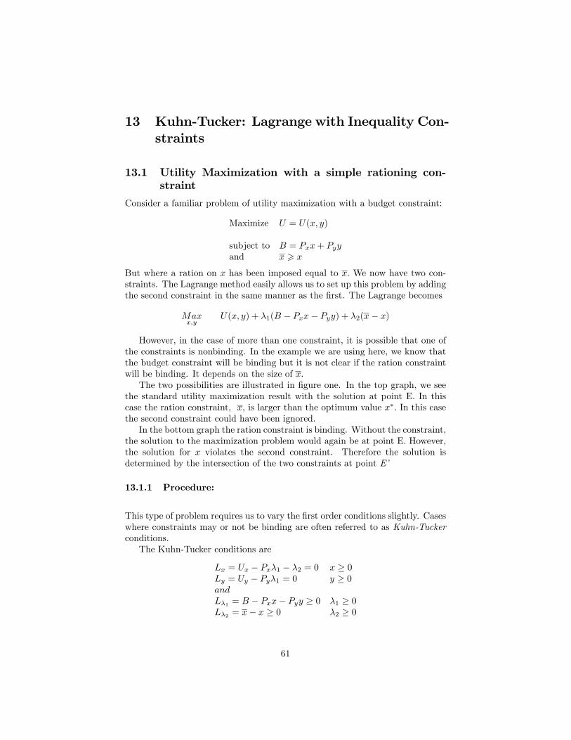
However, in the case of more than one constraint, it is possible that one ofthe constraints is nonbinding. In the example we are using here, we know thatthe budget constraint will be binding but it is not clear if the ration constraintwill be binding. It depends on the size of x.The two possibilities are illustrated in figure one. In the top graph, we see
the standard utility maximization result with the solution at point E. In thiscase the ration constraint, x, is larger than the optimum value x∗. In this casethe second constraint could have been ignored.In the bottom graph the ration constraint is binding. Without the constraint,
the solution to the maximization problem would again be at point E. However,the solution for x violates the second constraint. Therefore the solution isdetermined by the intersection of the two constraints at point E’
13.1.1 Procedure:
This type of problem requires us to vary the first order conditions slightly. Caseswhere constraints may or not be binding are often referred to as Kuhn-Tuckerconditions.The Kuhn-Tucker conditions are
Lx = Ux − Pxλ1 − λ2 = 0 x ≥ 0Ly = Uy − Pyλ1 = 0 y ≥ 0andLλ1 = B − Pxx− Pyy ≥ 0 λ1 ≥ 0Lλ2 = x− x ≥ 0 λ2 ≥ 0
61

y
x
U0
U1
E
BPy
BPx= x*
y*
Case 2: Second constraintis Binding
x
y
U0
U1
Maximize U = U(x,y)
subject to B = Pxx + Pyy
and x < X
E
BPy
B Px
x*
y*
CASE 1: Secondconstraint Not Binding
X
X
E’
Now let us interpret the Kuhn-Tucker conditions for this particular problem.Looking at the Lagrange
U(x, y) + λ1(B − Pxx− Pyy) + λ2(x− x)
We require thatλ1(B − Pxx− Pyy) = 0
therefore eitherλ1 = 0or
B − Pxx− Pyy = 0
If we interpret λ1as the marginal utility of the budget (Income), then ifthe budget constraint is not met the marginal utility of additional B is zero(λ1 = 0).(2) Similarly for the ration constraint, either
x− x = 0or
λ2 = 0
λ2 can be interpreted as the marginal utility of relaxing the ration constraint.
62

13.1.2 Solving by Trial and Error
Solving these types of problems is a bit like detective work. Since there are morethan one possible outcomes, we need to try them all. But before you start, itis important to think about the problem and try to make an educated guess asto which constraint is more likely to be nonbinding. In this example we can besure that the budget constraint will always be binding, therefore we only needto worry about the effects of the ration constraint.
Step one: Assume λ2 = 0, λ1 > 0 (simply ignore the second constraint)the first order conditions become
Lx = Ux − Pxλ1 − λ2 = 0Ly = Uy − Pyλ1 = 0Lλ1 = B − Pxx− Pyy = 0
Find a solution for x∗ and y∗ then check if you have violated the constraint youignored. If you have, go to step two.Step two: Assume λ2 > 0, λ1 > 0 (use both constraints, assume they are
binding)The first order conditions become
Lx = Ux − Pxλ1 − λ2 = 0Ly = Uy − Pyλ1 = 0Lλ1 = B − Pxx− Pyy = 0Lλ2 = x− x = 0
In this case, the solution will simply be where the two constraints intersect.Step three: Assume λ2 > 0, λ1 = 0 (use the second constraint, but ignore
the first constraint)
Numerical exampleMaximize U = xy
subject to:100 ≥ x+ y
andx ≤ 40
The Lagrange is
xy + λ1(100− x− y) + λ2(40− x)
and the Kuhn-Tucker conditions become
Lx = y − λ1 − λ2 = 0 x ≥ 0Ly = x− λ1 = 0 y ≥ 0Lλ1 = 100− x− y ≥ 0 λ1 ≥ 0Lλ2 = 40− x ≥ 0 λ2 ≥ 0
63

Which gives us four equations and four unknowns: x, y, λ1 and λ2.To solve, we typically approach the problem in a stepwise manner. First,
ask if any λi could be zero Try λ2 = 0 (λ1 = 0 does not make sense, given theform of the utility function), then
x− λ1 = y − λ1 or x = y
from the constraint 100−x−y we get x∗ = y∗ = 50 which violates our constraintx ≤ 40. Therefore x∗ = 40 and y∗ = 60, also λ∗1 = 40 and λ∗2 = 20
13.2 War-Time Rationing
Typically during times of war the civilian population is subject to some form ofrationing of basic consumer goods. Usually, the method of rationing is throughthe use of redeemable coupons used by the government. The government willsupply each consumer with an allotment of coupons each month. In turn, theconsumer will have to redeem a certain number of coupons at the time of pur-chase of a rationed good. This effectively means the consumer ”pays” two”prices” at the time of the purchase. He or she pays both the coupon priceand the monetary price of the rationed good. This requires the consumer tohave both suffi cient funds and suffi cient coupons in order to buy a unit of therationed good.Consider the case of a two-good world where both goods, x and y. are
rationed. Let the consumer’s utility function be U = U(x, y). The consumerhas a fixed money budget of B and faces the money prices Px and Py. Further,the consumer has an allotment of coupons, denoted C, which can be used topurchase both x or y at a coupon price of cx and cy. Therefore the consumer’smaximization problem isMaximize
U = U(x, y)
Subject toB ≥ Pxx+ Pyy
andC ≥ cxx+ cyy
in addition, the non-negativity constraint x ≥ 0 and y ≥ 0.The Lagrangian for the problem is
Z = U(x, y) + λ(B − Pxx− Pyy) + λ2(C − cxx+ cyy)
where λ, λ2 are the Lagrange multiplier on the budget and coupon con-straints respectively. The Kuhn-Tucker conditions are
Zx = Ux − λ1Px − λ2cx = 0Zy = Uy − λ1Py − λ2cy = 0Zλ1 = B − Pxx− Pyy ≥ 0 λ1 ≥ 0Zλ2 = C − cxx− cyy ≥ 0 λ2 ≥ 0
64

Numerical ExampleLet’s suppose the utility function is of the form U = x · y2. Further, let
B = 100, Px = Py = 1 while C = 120 and cx = 2, cy = 1.The Lagrangian becomes
Z = xy2 + λ1(100− x− y) + λ2(120− 2x− y)
The Kuhn-Tucker conditions are now
Zx = y2 − λ1 − 2λ2 ≤ 0 x ≥ 0 x · Zx = 0Zy = 2xy − λ1 − λ2 ≤ 0 y ≥ 0 y · Zy = 0Zλ1 = 100− x− y ≥ 0 λ1 ≥ 0 λ1 · Zλ1 = 0Zλ2 = 120− 2x− y ≥ 0 λ2 ≥ 0 λ2 · Zλ2 = 0
Solving the problem:Typically the solution involves a certain amount of trial and error. We first
choose one of the constraints to be non-binding and solve for the x and y. Oncefound, use these values to test if the constraint chosen to be non-binding isviolated. If it is, then redo the procedure choosing another constraint to benon-binding. If violation of the non-binding constraint occurs again, then wecan assume both constraints bind and the solution is determined only by theconstraints.Step one: Assume λ2 = 0, λ1 > 0By ignoring the coupon constraint, the first order conditions become
Zx = y2 − λ1 = 0Zy = 2xy − λ1 = 0Zλ1 = 100− x− y = 0
Solving for x and y yields
x∗ = 33.33 y∗ = 66.67
However, when we substitute these solutions into the coupon constraint wefind that
2(33.33) + 66.67 = 133.67 > 120
The solution violates the coupon constraints.Step two: Assume λ1 = 0, λ2 > 0Now the first order conditions become
Zx = y2 − 2λ2 = 0Zy = 2xy − λ2 = 0Zλ1 = 120− 2x− y = 0
Solving this system of equations yields
x∗ = 20 y∗ = 80
65

When we check our solution against the budget constraint, we find that thebudget constraint is just met. In this case, we have the unusual result that thebudget constraint is met but is not binding due to the particular location of thecoupon constraint. The student is encouraged to carefully graph the solution,paying careful attention to the indifference curve, to understand how this resultarose.
13.3 Peak Load Pricing
Peak and off-peak pricing and planning problems are common place for firmswith capacity constrained production processes. Usually the firm has investedin capacity in order to target a primary market. However there may exist asecondary market in which the firm can often sell its product. Once the capitalhas been purchased to service the firm’s primary market, the capital is freelyavailable (up to capacity) to be used in the secondary market. Typical exam-ples include: schools and universities who build to meet day-time needs (peak),but may offer night-school classes (off-peak); theatres who offer shows in theevening (peak) and matinees (off-peak); or trucking companies who have dedi-cated routes but may choose to enter ”back-haul”markets. Since the capacityprice is a factor in the profit maximizing decision for the peak market and isalready paid, it normally, should not be a factor in calculating optimal price andquantity for the smaller, off-peak market. However, if the secondary market’sdemand is close to the same size as the primary market, capacity constraintsmay be an issue, especially given that it is common practice to price discrim-inate and charge lower prices in off-peak periods. Even though the secondarymarket is smaller than the primary, it is possible at the lower (profit maximiz-ing) price that off-peak demand exceeds capacity. In such cases capacity choicesmaust be made taking both markets into account, makeing the problem a classicapplication of Kuhn-Tucker.Consider a profit maximizing Company who faces two demand curves
P1 = D1(Q1) in the day time (peak period)P2 = D2(Q2) in the night time (off-peak period)
to operate the firm must pay b per unit of output, whether it is day or night.Furthermore, the firm must purchase capacity at a cost of c per unit of output.Let K denote total capacity measured in units of Q. The firm must pay forcapacity, regardless if it operates in the off peak period. Question: Who shouldbe charged for the capacity costs? Peak, off-peak, or both sets of customers?The firm’s maximization problem becomes
MaximizeQ1,Q2,K
P1Q1 + P2Q2 − b(Q1 −Q2)− cK
Subject toK ≥ Q1
K ≥ Q2
66

WhereP1 = D1(Q1)P2 = D2(Q2)
The Lagrangian for this problem is:
Z = D1(Q1)Q1 +D2(Q2)Q2 − b(Q1 +Q2)− cK + λ1(K −Q1) + λ2(K −Q2)
The Kuhn-Tucker conditions are
Z1 = D1 +Q1∂D1
∂Q1− b− λ1 = 0 (MR1 − b− λ1 = 0)
Z2 = D2 +Q2∂D2
∂Q2− b− λ2 = 0 (MR2 − b− λ2 = 0)
ZK = −c+ λ1 + λ2 = 0 (c = λ1 + λ2)Zλ1 = K −Q1 ≥ 0 λ1 ≥ 0Zλ2 = K −Q2 ≥ 0 λ2 ≥ 0
Assuming that Q1, Q2,K > 0 the first-order conditions become
MR1 = b+ λ1 = b+ c− λ2 (λ1 = c− λ2)MR2 = b+ λ2
Finding a solution:Step One: Since D2(Q2) is smaller than D1(Q1) try λ2 = 0Therefore from the Kuhn-Tucker conditions
MR1 = b+ c− λ2 = b+ cMR2 = b+ λ2 = b
which implies that K = Q1. Then we check to see if Q∗2 ≤ K. If true, thenwe have a valid solution. Otherwise the second constraint is violated and theassumption that λ2 = 0 was false. Therefore we proceed to the next step.Step Two: if Q∗2 > K then Q∗1 = Q∗2 = K and
MR1 = b+ λ1
MR2 = b+ λ2
Since c = λ1 + λ2 then λ1 and λ2 represent the share of c each group pays.Both cases are illustrated in figure 13.3
Numerical Example Suppose the demand during peak hours is
P1 = 22− 10−5Q1
and during off-peak hours is
P2 = 18− 10−5Q2
67

MR1MR2
Q1, Q2, K
b
b+c
$
Q1 =KQ2 < K
E1
E2
MR1MR2
Q1, Q2, K
b
b+c
$
Q1 = Q2 = K
E1
E2λ2
λ1
Case 1: Offpeak constraint nonbinding Case 2: Offpeak constraint binding
To produce a unit of output per half-day requires a unit of capacity costing8 cents per day. The cost of a unit of capacity is the same whether it is used atpeak times only or off-peak also. In addition to the costs of capacity, it costs 6cents in operating costs (labour and fuel) to produce 1 unit per half day (bothday and evening)If we assume that the capacity constraint is binding (λ2 = 0), then the
Kuhn-Tucker conditions (above) become
λ1 = c = 8MR︷ ︸︸ ︷
22− 2× 10⁻⁵Q1
MC︷ ︸︸ ︷= b+ c = 14
18− 2× 10⁻⁵Q2 = b = 6
Solving this system gives us
Q1 = 40000
Q2 = 60000
which violates the assumption that the second constraint is non-binding (Q2 >Q1 = K).Therefore, assuming that both constraints are binding, then Q1 = Q2 = Q
and the Kuhn-Tucker conditions become
λ1 + λ2 = 8
22− 2× 10⁻⁵Q = 6 + λ1
18− 2× 10⁻⁵Q = 6 + λ2
which yields the following solutions
Q = K = 50000
λ1 = 6 λ2 = 2
P1 = 17 P2 = 13
Since the capacity constraint is binding in both markets, market one pays λ1 = 6of the capacity cost and market two pays λ2 = 2.
68

13.4 Problems
1. Suppose in the above example a unit of capacity cost only 3 cents per day.
(a) What would be the profit maximizing peak and off-peak prices andquantitites?
(b) What would be the values of the Lagrange multipliers? What inter-pretation do you put on their values?
2. Skippy lives on an island where she produces two goods, x and y, accordingthe the production possibility frontier 200 ≥ x2 + y2, and she consumesall the goods herself. Her utility function is
u = x · y3
Skippy also faces and environmental constraint on her total output of bothgoods. The environmental constraint is given by x+ y ≤ 20
(a) Write down the Kuhn Tucker first order conditions.
(b) Find Skippy’s optimal x and y. Identify which constaints are binding.
3. An electric company is setting up a power plant in a foreign country andit has to plan its capacity. The peak period demand for power is given byp1 = 400− q1 and the off-peak is given by p2 = 380− q2. The variable costto is 20 per unit (paid in both markets) and capacity costs 10 per unitwhich is only paid once and is used in both periods.
(a) write down the lagrangian and Kuhn-Tucker conditions for this prob-lem
(b) Find the optimal outputs and capacity for this problem.
(c) How much of the capacity is paid for by each market (i.e. what arethe values of λ1 and λ2)?
(d) Now suppose capacity cost is 30 per unit (paid only once). Findquantities, capacity and how much of the capacity is paid for by eachmarket (i.e. λ1 and λ2)?
69