Bringing Actuarial Measures of Defined Benefit Pensions into the U.S. National Accounts

Marshall Reinsdorf (International Monetary Fund)

David Lenze (U.S. Bureau of Economic Analysis)

Dylan Rassier (U.S. Bureau of Economic Analysis)

Paper Prepared for the IARIW 33rd

General Conference

Rotterdam, the Netherlands, August 24-30, 2014

Session 8B

Time: Friday, August 29, Afternoon

Bringing Actuarial Measures of Defined Benefit Pensions into the U.S. National Accounts*

Marshall B. Reinsdorf

International Monetary Fund

Washington, DC

mreinsdorf@imf.org

David G. Lenze

U.S. Bureau of Economic Analysis

Washington, DC

david.lenze@bea.gov

Dylan G. Rassier

U.S. Bureau of Economic Analysis

Washington, DC

dylan.rassier@bea.gov

July 2014

Abstract: The 1993 System of National Accounts (SNA93) uses a cash approach to measure household

income from participation in employer-sponsored defined benefit (DB) pension plans. In particular,

SNA93 uses actual employer contributions to pension plans and actual property income earned on

assets held by pension plans to measure household income. In contrast, the 2008 System of National

Accounts (SNA2008) bases its measures of household income from DB plans on actuarial estimates of

the net present value of benefit entitlements. The sources of increase in the actuarial value of benefit

entitlements that count as income to households are credit for additional service to the employer and

interest accruing on accumulated benefit entitlements. As part of the July 2013 comprehensive revision

of the U.S. National Income and Product Accounts, the Bureau of Economic Analysis changed the

accounting for DB pension plans from a cash basis under SNA93 to an accrual basis under SNA2008.

This paper reviews the U.S. experience with the new accrual accounting treatment.

JEL Codes: D24, E01

Keywords: production, measurement, national accounts

* Questions about this paper should be directed to Dylan Rassier. The views expressed in this paper are solely those of the

authors and should not be attributed to the International Monetary Fund or its Executive Board or management, or to the

U.S. Department of Commerce. Marshall Reinsdorf was chief of the national accounts research group at the Bureau of

Economic Analysis when the research for this paper was done.

1

1. Introduction

A defined benefit (DB) pension plan is an employment-related retirement scheme in which the

benefit to be paid in retirement is determined by a formula, such as length of service to the employer

times final salary times an accrual rate. The 1993 System of National Accounts (SNA93) measures

income that households receive from participating in DB pension plans by actual employer

contributions to DB pension plans and property income earned on assets held by DB pension plans.

Thus, SNA93 uses cash measures that treated DB pension plans as property of the household sector.

The 2008 System of National Accounts (SNA2008) takes a different approach, however. A key

innovation in SNA2008 is accounting for the income that households receive as participants in DB

pension plans based on the change in the net present value of future benefit entitlements arising from

credit for additional years of service to the employer and from the shortening of the waiting period

over which future benefits are discounted.2 By using actuarial estimates of these concepts, DB pension

plans can be measured on an accrual basis.

Accrual measures of DB pension transactions have some important advantages over cash

measures. First, cash measures often fail to reflect the timing of when pension-related compensation is

earned. Even though employees usually accrue future benefits in a smooth manner, actual employer

contributions can vary widely over time both because of the impact on required contributions of

swings in market values of equities and because actual contributions can lag behind and be lumpier

than required contributions. Second, the property income earned on pension plan assets can diverge

from the interest accruing on accumulated benefit entitlements because of a gap between the values of

the assets and the benefit entitlements or a gap between the average yield of the assets and the interest

rate assumed in the actuarial calculations. Equity assets typically have low dividend yield rates

2 The change in the present value of a future payment caused by discounting by one year less equals the interest rate times

the original present value of the payment, so in effect, households earn interest on the opening value of their benefit

entitlement.

2

because they generate part of their investment returns from holding gains, but holding gains are not

included in the definition of property income that is appropriate for national accounts purposes. The

exclusion of holding gains reduces the cash measure of DB pension saving of households.

The U.S. Bureau of Economic Analysis (BEA) changed the method of accounting for DB

pension income from a cash basis under SNA93 to an accrual basis under SNA2008 as part of the 2013

comprehensive revision of the U.S. National Income and Product Accounts (NIPAs) (Smith and

Holdren, 2013, and Kornfeld, 2013). In addition to introducing the new accounting treatment, new

tables were introduced showing the transactions of the DB pension plan subsector and a breakout of

this subsector by the type of employer sponsoring the pension plan: business (or private) sector, state

and local government sector, and federal government sector.

This paper provides a comprehensive summary of methods and data sources used to implement

the accrual approach to DB pension plans in the U.S. NIPAs and a review of the U.S. experience with

the new measures. It begins with general background information on DB pension plans. Then it

outlines SNA93 recommendations and SNA2008 recommendations, focusing on some conceptual

questions that arose during implementation in the U.S. NIPAs. Third, it describes the source data and

estimation methods used for each kind of employer. Fourth, it present results and discusses the effects

of the new measurement approach on the estimates of household income, saving, and wealth and on

saving by employer sectors. A summary and overview of topics for future research concludes the

paper.

2. Background on Defined Benefit Pensions

This section reviews DB pension concepts that are relevant to the new accrual accounting

treatment and describes two categories of actuarial methods that could be used to estimate benefit

entitlements. The section also describes the institutional characteristics of DB pensions in the U.S.

3

2.1. Defined Benefit Pension Concepts

From an economic perspective, an employee covered by a DB pension plan accepts lower

compensation for services rendered in the current period in exchange for an employer’s promise to pay

future pension benefits related to the services. Thus, a DB pension is a form of deferred compensation,

and the employer incurs a liability associated with the pension cost. The periodic pension cost is

estimated by applying actuarial methods to data on age, years of service, and other characteristics of

the participants in the DB pension. In business accounting, the periodic pension cost includes

components that reflect income earned in production and also components that reflect revaluations of

assets or other changes in the volume of assets. For national economic accounting purposes, however,

the periodic pension cost only includes the components that reflect income earned in production:

normal cost and interest cost.

The normal cost (or service cost) component reflects the actuarial value of the benefit

entitlements earned through service to the employer in the current period. The normal cost may not be

borne entirely by the employer; often the employees are required to make contributions to the pension

plan. The employer normal cost is then the residual that remains after subtracting employee

contributions from total normal cost.

The interest cost component reflects interest earned in the current period on accumulated

benefit entitlements for services rendered in past periods. If the pension plan is unfunded (meaning

that there is no trust fund holding assets) the accumulated benefit entitlements can be thought of as a

loan from households to employers. As with any loan, an interest cost accrues on the unpaid balance.

The interest cost would equal the interest rate times the opening value of the benefit entitlements.

In principle, an employer ought to be able to avoid the interest cost if the employer pays the

employer normal cost when it is accrued. A pension fund (or pension plan) is a separate institutional

unit that can receive such payments from the employer. In particular, if the employer and employees

4

make timely contributions to a pension fund equal to the normal cost, in principle the pension fund

ought to be able to earn enough property income and investment returns from holding gains to cover

the interest cost. In the United States, almost all DB pension plans are funded. Furthermore, most of

the discussion of DB pensions in the SNA2008 assumes that the pension plan is funded and that it can

be treated as a separate institutional unit that is directly responsible for paying the benefits (albeit with

the ultimate backing of the plan sponsor or “pension manager”). The SNA2008 therefore treats the

interest income of households as an interest expense of the pension plan sector and shows households

as returning their interest income to the pension plan in the form of contribution supplements.

The actuarial liability is a commonly used term for the value of the accumulated benefit

entitlements. If the projections that underlie the actuarial calculations are, in fact, realized, and there

are no changes in actuarial assumptions or plan rules, the change in actuarial liability may be found by

adding the normal cost and interest cost for the period and subtracting the benefit payments and

withdrawals for the period. However, changes in the actuarial liability may result from changes in

actuarial assumptions such as the discount rate, from amendments to the pension contract such as

changes in the benefit formula, or from differences between actual experience and previous actuarial

assumptions (i.e., experience gains and losses). The expression for the change in actuarial liability is:

(2.1) Change in actuarial liability = normal cost + interest cost – benefit payments + / – (actuarial

assumptions, amendments, experience gains and losses).

Assets held by the pension plan, or pension plan assets, reflect the market value of all resources

available to satisfy the actuarial liability. For any given period, the change in pension assets may be

determined by adding contributions from employers and employees and property income earned on

pension assets for the period and subtracting benefit payments and withdrawals and administrative

expenses related to operating the pension plan for the period. In addition, changes in pension assets

5

may result from holding gains and losses or from capital transfers. The change in pension plan assets

is summarized as follows:

(2.2) Change in pension plan assets = employer contributions + employee contributions + property

income – benefit payments – administrative expenses + / – (holding gains and losses, capital

transfers).

The difference between the actuarial liability and pension plan assets is referred to as the

unfunded actuarial liability or simply the UAL. If the actuarial liability exceeds the pension plan’s

assets, the UAL is positive. The expression for the UAL is:

(2.3) UAL = actuarial liability – pension plan assets.

A common measure of funding status for DB pension plans is the funding ratio, which is

calculated as:

(2.4) Funding ratio = pension plan assets

actuarial liability

If the funding ratio is less than one, the plan is underfunded; if it is greater than one, the plan is

overfunded.

2.2. Actuarial Methods

The SNA2008 summarizes two broad categories of actuarial methods from business accounting

that can be used to value the normal cost and the actuarial liability: the projected benefit obligation

(PBO) approach, and accrued benefit obligation (ABO) approach. The ABO approach is more

consistent with the accounting concept of a liability, as it does not include future transactions that

potentially could be avoided by an employer in a situation of financial distress.3 Yet the PBO

3 Brown and Wilcox (2009, p. 540) observe that “One reason for favoring the ABO is that it is the one measure of liability

that puts pension benefits and salaries on the same footing. In financial reports, employers are required to disclose the

aggregate salaries their employees have earned by the close of the reporting period; they are not required to recognize

6

approach also has advantages, and no consensus exists regarding the choice of actuarial method

(Wilcox 2006).

Despite the murky state of the debate over whether to use ABO or PBO, there are some clear

principles that can guide the choice. To understand the practical implications of each approach,

consider a traditional DB pension benefit formula that equates the benefit with final pay, or average

final pay, times the length of the career times a fixed percentage replacement rate. With this kind of

formula, salary increases raise the value of the pension. We can either account for the salary growth

effect on an ex post basis, or make a projection of future salary increases and incorporate them into the

value of the benefits being earned today.

The ABO actuarial liability equals the present value of benefits that would be due to

participants if the pension plan were to be frozen on the valuation date, so ABO methods reflect salary

growth on an ex post basis. The ABO normal cost for a year includes both the effect of credit for an

additional year of service and the effect of pay raises received during the year. If the benefit level

depends on final pay, the effect of a pay raise on the value of the benefit entitlement will be large for

participants who have accumulated credit for many years of service. As a result, ABO methods tend to

yield relatively high estimates of normal cost in the last years of the career and relatively low estimates

of accumulated participant wealth in the early and middle years of the career. The average level of

periodic normal cost over the course of the career must be higher because the back-loading of normal

cost implies that less time is available to accumulate property income. Thus, when applied to a

population that includes employees at all points in their career, ABO methods yield relatively high

estimates of compensation and relatively low estimates of property income for households.

PBO methods project the ultimate level of benefit entitlements including the effects of

projected future salary increases related to general wage inflation and additional years of experience.

salaries that will be earned in future periods even though today’s workers may have a high probability of remaining in their

jobs after the current reporting period is over.”

7

Allowing for projected future pay raises yields higher estimates of normal cost for participants in the

early years of their careers than under ABO methods, and it yields higher estimates of accumulated

wealth for employed participants not at the end of their careers. Thus, PBO methods tend to yield

lower estimates of compensation and higher estimates of property income for households than under

ABO methods. Note that at the time of retirement both approaches yield the same estimate of benefit

entitlements, so they tend to yield the same total pension income of households, differing only in how

they split the total into normal cost and interest cost components.

One criterion for choosing between an ABO method and a PBO method is whether participants

in the pension plan effectively have a secure right to accrue additional benefits and to gain from future

pay raises.4 Private business sector sponsors of DB pension plans in the U.S. are permitted to freeze or

terminate their plans at will, depriving participants of the opportunity to accrue additional benefit

entitlements. (Employers who terminate their DB plan usually replace it with a defined contribution

(DC) plan to which they make contributions, but the value of the DC plan is often less.) Because

neither law nor custom obligates the business sector sponsor to give participants future opportunities to

accrue benefits, ABO methods are appropriate for measuring the DB pension income of private

business sector participants in the U.S.

In general, employees of U.S. state and local governments have a secure right to continue to

accrue benefits in the future years of their careers under the formula in effect when they were hired.

Protections against increases in required employee contributions are weaker, however, and as pension

costs have begun to be a source of financial stress for many state and local governments, a number of

states have raised member contribution rates or reduced the automatic cost of living adjustments

4 As discussed in Reinsdorf and Lenze (2009), models of the option value of pensions in Lazear and Moore (1988) and

Stock and Wise (1990) imply that the right to accrue future benefits is a valuable asset if the probability of a plan freeze or

plan termination is low. In a plan freeze the pension plan continues to exist in order to pay benefits due to retirees, while in

a plan termination the employer pays a life insurance company to take over the responsibility of paying the benefits or pays

a lump sum to plan participants with small benefit entitlements.

8

(COLAs) to the pension benefits paid to current retirees.5 Also, in some cases, benefits have been

reduced as part of a court-approved restructuring of the liabilities of bankrupt local governments.6

Thus, the facts that once favored PBO methods for DB pension plans sponsored by U.S. state and local

governments are now more ambiguous, and ABO methods seem more reasonable.7 Nevertheless,

given the security of rights to accrue future benefits under the same plan rules for employees of the

U.S. federal government, PBO methods are still reasonable for measuring these plans.8

Using the same method for all sectors in the U.S. NIPAs would make compensation estimates

and property income estimates more comparable across sectors, but there are also practical

considerations. In the U.S., source data on actuarial measures of DB pension plans are available, but

they differ between sectors. The source data for the business sector are based on an ABO method

while source data for the government sectors are based on PBO methods. To enforce consistency

would require the conversion of source data for the business sector from ABO to PBO or the

conversion of source data for the government sectors from PBO to ABO. In the end, we decided to

convert from PBO to ABO for the state and local government sector only.9

2.3. Institutional Characteristics of U.S. Defined Benefit Pensions

A challenge in developing a single set of international standards for employment-related

pension schemes in SNA2008 is the diversity of pension institutions that exist in different countries.

To explore the implications of institutional diversity, Durant, Lenze, and Reinsdorf (2010) develop

actuarial measures of DB pensions and social security pensions for two countries that reflect two poles

5 Examples of states reducing COLAs for current retirees include Colorado, Illinois, Minnesota, New Jersey, New Mexico,

Rhode Island, and South Dakota. Examples of states raising member contribution rates include Florida, New Hampshire

and Virginia. The Florida Retirement System, which formerly was a noncontributory pension plan, now requires members

to contribute 3 percent of wages. Some changes are still being litigated in court. 6 Examples of local governments that have or are trying to reduce pension benefits for retirees through bankruptcy

proceedings include Detroit Michigan, San Bernardino California, Central Falls Rhode Island, and Prichard Alabama. 7 See also Gold and Latter (2008) for other grounds favoring the use of ABO methods for state and local governments.

8 Employee contribution rates were recently raised for newly hired federal civilian employees, but not for existing

employees. 9 Gold and Latter (2008) advocate the use of ABO methods for state and local government plans.

9

of institutional diversity—France and the U.S. Employer-sponsored pension plans predominate in the

U.S., whereas in France most DB pensions are government-sponsored. The authors demonstrate the

international comparisons that are made possible by the supplementary pension table in SNA2008,

which includes both employer-sponsored and government-sponsored plans. Here, we focus on the

institutional characteristics of U.S. DB pension plans.

In the U.S., three sectors of employers sponsor DB pension plans: 1) private business, 2) state

and local governments, and 3) the federal government. For purposes of measuring pensions, it is

convenient to include plans sponsored by public corporations with the plans that are sponsored by the

government that owns those public corporations. Each sector of pension plan sponsors has

institutional characteristics that are relevant for designing measurement procedures and for interpreting

the conceptual guidance of SNA2008. Institutional characteristics also matter for understanding the

different patterns of behavior exhibited by the different sectors. In particular, private sector pension

plans and many government sector pension plans are intended as supplements to social security, which

is a government social benefits plan for the broad population. These plans tend to have less generous

benefit formulas than the plans for government employees not covered by social security.

2.3.1. Characteristics of Private Defined Benefit Pensions

DB pension plans sponsored by businesses in the U.S. (i.e., a private plan) are funded at least in

part by contributions from employers, and may be funded by contributions from employees. Private

DB plans also receive property income earned and holding gains generated by actual assets, which

usually consist of a mix of equity assets and interest-bearing assets. Employer contributions are driven

in part by federal funding requirements under the Employee Retirement Income Security Act of 1974

(ERISA) and by follow-on legislation, including the Pension Protection Act of 2006. Under ERISA, a

private DB pension sponsor incurs a penalty if the funding ratio falls below a minimum threshold;

likewise, the deductibility of contributions for income tax purposes is offset by an excise tax if the

10

funding ratio exceeds a maximum threshold. Employer contributions are also driven in part by

accounting rules under U.S. generally accepted accounting principles (GAAP) for nongovernmental

entities. U.S. GAAP requires a private DB pension sponsor to report on financial statements a liability

to reflect any unfunded benefit entitlements. Thus, an employer has incentives to make contributions

in cases of inadequate funding and incentives to limit contributions in cases of excess funding. The

resulting inverse relationship between the funding ratio and employer contributions can generate

volatility in the employers’ actual contributions.

In addition to establishing funding requirements and other regulatory requirements, ERISA

created the Pension Benefit Guaranty Corporation (PBGC), a federal agency that insures benefit

entitlements for participants in almost all private DB pension plans. The PBGC is funded by insurance

premiums paid by private plan sponsors and the investment income from the assets of the plans that

have entered into PBGC trusteeship. As a percentage of assets held by private DB pension plans, over

98 percent of the plans are covered under PBGC insurance in recent years.

Each private plan sponsor subject to ERISA is required to file tax form 5500 with its federal

income tax return for each plan sponsored. Form 5500 is an annual report that contains financial

information and actuarial information on individual plans. Data bases of form 5500 filings are

compiled by the Employee Benefits Security Administration (EBSA) of the U.S. Department of Labor

and by the PBGC. The EBSA tabulates the financial (cash) measures of DB pension plans from form

5500 and publishes the totals. The actuarial measures are included in the PBGC data base. The U.S.

NIPAs use the information published by the EBSA and also the PBGC databases in compiling

estimates of the transactions of private DB plans.

Although pension plan participants have property rights to the benefits that they have already

accrued (and insurance from the PBGC against loss of these benefits in the event that the plan is

underfunded and its sponsor goes bankrupt), private DB plans may be frozen or terminated at the will

11

of the sponsor. Indeed, a longstanding trend among existing businesses has been to replace their DB

pension plan with a DC pension plan. Furthermore, new businesses almost inevitably choose a DC

plan rather than a DB plan as a retirement benefit. As a result of these trends, the number of private

DB plans and the number of participants in these plans have both been on a gradual decline since the

passage of ERISA. The number of private pension plans peaked at 175,143 in 1983 and declined to

45,256 in 2011. The number of active and retired participants covered by private DB plans peaked

more recently at 42.3 million in 2008, but the number of active participants peaked at 30.1 million in

1984 and declined to 16.5 million in 2011. As a percent of private, full-time equivalent employment,

active participants covered by private DB plans peaked at 45.4 percent in 1975 and declined to 16.2

percent in 2011.

2.3.2. Characteristics of State and Local Government Defined Benefit Pensions

Most DB pension plans sponsored by a state or local government are funded by a combination

of contributions from employers and from members (i.e., employees), property income earned on plan

assets, and holding gains on plan assets. Member contributions are set as a percentage of pay. State

and local government plans are not insured by PBGC, nor are they subject to ERISA reporting

requirements (they do not file Form 5500) and requirements mandating minimum employer

contributions. Instead, financial reporting standards for state and local government plans are set by the

Governmental Accounting Standards Board (GASB), and the degree of underfunding of these pension

plans reflects the legal, political, and economic environments of the various state and local

governments. GASB currently prohibits the use of ABO actuarial methods and mandates the use of

one of six variants of PBO methods.10

Although private DB plans are on the decline, for state and local government employees DB

pension plans continue to be the predominant form of retirement plan. Furthermore, many state and

10

Many accounting standards will change when GASB Statement 67, adopted in June 2012, is implemented.

12

local government employees are not covered by federal social security.11

In 2012, there were 227

state-administered and 3,771 locally-administered DB pension plans according to the Survey of Public

Pension Plans conducted by the U.S. Census Bureau. The number of active state and local plan

members was 14.4 million (91 percent of the 15.9 million full-time equivalent employees), and the

number of beneficiaries receiving periodic benefit payments was 9.0 million.

2.3.3. Characteristics of Federal Government Defined Benefit Pensions

The U.S. federal government sponsors approximately 40 DB pension plans, but the two general

plans for civilian personnel and the military plan together comprise over 95 percent of the federal

pension system. The civilian plans receive contributions from the federal government in its role as the

employer and from the employees, but in the main civilian plan, known as the Federal Employee

Retirement System (FERS), the employee contributions are relatively small. The military plan is

funded solely by the employer.

The main federal plans also receive interest income from assets; however, in contrast to private

plans and state and local plans, the assets held by federal plans consist almost entirely of interest-

bearing U.S. Treasury securities, which pay interest and do not generate holding gains.12

The first large federal civilian DB plan, known as the Civil Service Retirement System (CSRS),

was started in 1920. It was an unfunded plan that operated on a pay-as-you-go basis until 1969, when

provisions to begin funding it on an ABO basis were passed by Congress. Similarly the military

pension plan operated as an unfunded plan from 1935 to 1984 (before 1935 it was partially funded).

After 1984 normal costs as estimated using a PBO approach were contributed to the military pension

plan by the employer, and the law that established the military pension trust fund also called for

“catch-up” contributions from the federal government to amortize the UAL inherited from prior years.

11

According to Brainard (2006, p.7), “Approximately one-fourth of all employees of state and local government do not

participate in Social Security, including nearly one-half of all public school teachers and most or substantially all public

employees in Alaska, Colorado, Louisiana, Maine, Massachusetts, Ohio, and Nevada.” 12

The military plan bought some inflation-proteced TIPS bonds that could rise in price if inflation were to accelerate.

13

However, in practice the catch-up contributions have generally been about sufficient to cover the

interest accruing on the UAL, preventing it from growing even larger, but not large enough to bring it

down. Similarly, on the civilian side, the Federal Employees’ Retirement Act of 1986, which created

FERS, calls for the employer contribution rates to be set at a level that will keep the plan fully funded

on a PBO basis and for payments to amortize the ABO UAL of the CSRS plan. However, the

amortization payments have tended to approximately cover the interest accruing on the PBO UAL, but

not large enough to make the PBO UAL fall by any appreciable amount. In particular, the large legacy

of unfunded pension obligations in both CSRS and the military plan from before the reforms of the

mid-1980s are being amortized so slowly that in recent years the federal plans have tended to be

consistently around 40 percent funded on a PBO basis.

FERS benefits are much less generous than CSRS benefits because FERS employees

participate in social security and because FERS employees also have a DC pension plan, known as the

Thrift Savings Plan (TSP), to which the employer contributes of up to 5 percent of pay. After 10 years

of service, for each additional year of service most employees in CSRS earn benefit entitlements equal

to 2 percent of their average pay in the highest paid three years of their career (usually the last three

years). Most employees in FERS get a benefit of 1 percent of their “high-three” average pay per year

of service, or 1.1 percent per year of service if they retire at age 62 or later. Employees in CSRS or the

military plan do not make contributions to social security or receive social security benefits.

Federal DB plans do not file form 5500, but the actuaries at the Office of Personal Management

(a federal agency) prepare an annual report on the two large civilian plans, and actuaries at the

Department of Defense prepare an annual report on the main military plan. These annual reports

include financial information and detailed actuarial information on a PBO basis that we use to

calculate the estimates for the main federal plans.

14

We do not attempt to make precise estimates for the smaller federal plans based on the specifics

of their operations, but rather simply assume that they are a fixed proportion of the main federal plans.

In 1996 to 2011, the total pay of the civilian employees who were not in CRSR or FERS averaged

around 2.8 percent of the total pay of those who were in one of those plans, and the total pay of those

in the smaller military plans averaged about 2 percent of those of in the main plan. To adjust for the

smaller civilian plans, the estimates from the main civilian plans are therefore blown up by 2.8 percent,

and to adjust for the small military plans the estimates for the main plan are blown up by 2 percent.

3. Measurement of Defined Benefit Pensions in National Economic Accounts

In this section, we outline recommendations in SNA93 and in SNA2008 for the measurement of

income and saving attributable to employment-related DB pension plans. In addition to highlighting

changes introduced in SNA2008, we discuss our interpretation of the conceptual intent of SNA2008 and

the modifications of its procedural recommendations that are appropriate for the institutional

environment of the U.S and consistent with this conceptual intent.

3.1. Defined Benefit Pensions in the 1993 System of National Accounts

Annex IV of SNA93 summarizes the treatment of pensions. In SNA93, a pension plan is treated

as a pass-through institutional unit in the financial corporations sector that engages in financial

transactions on behalf of pension participants. Assets held by the pension plan are treated as property

of the participants. Unlike SNA2008, SNA93 does not measure claims to benefits earned by active

participants through service to employers. Thus, household compensation income attributable to DB

pension plans is measured by actual employer contributions to the plans. Likewise, household

property income attributable to DB pension plans is measured by property income earned on actual

assets held by the plans—i.e., interest, dividends, rents. Output of DB pension services is measured by

charges incurred to cover the costs of operating the plans, and households purchase the services as

15

final consumption.13

Based on the transactions summarized here, household saving before

redistributions is measured in SNA93 as follows:

(3.1) Household saving before redistributions = actual employer contributions + property income –

pension service charges.

Here “property income” is the income generated by the assets in the pension fund. Pension saving

before redistributions in SNA93 is zero because the pension plan is a pass-through institutional unit.

Both SNA93 and SNA2008 include redistributive transactions so that income can be recorded

both for households and for pension plans. Household income from employer contributions and

property income is redistributed from households back to the pension plan. In addition, employee

contributions to DB pension plans less pension service charges paid by employees are recognized as

distributions from households to the pension plan. Conversely, benefit payments are recognized as

distributions from the pension plan to households. Given these redistributive transactions, household

disposable income and pension saving, respectively, are measured in SNA93 as follows:

(3.2) Household saving after redistributions but before adjustment for change in net equity in

pension plans = benefit payments – employee contributions

and

(3.3) Pension plan saving after redistributions = actual employer contributions + property income +

(employee contributions – pension service charges) – benefit payments.

In measuring household saving, the expenditure on pension service charges that is included in

household disposable income is subtracted, and an “adjustment for the change in net equity of

households in pension funds” is added. This adjustment exactly equals pension plan saving. In

SNA93, pension plans are owned by the households that benefit from the plans. Once this ownership is

13

The SNA93 specifies that output of a pension plan is a service charge calculated as follows: output = total actual

contributions earned + total imputed contribution supplements – benefits due – change in pension reserves. However, the

change in pension reserves is calculated as follows: ∆ = total actual contributions earned + total imputed contribution

supplements – benefits due – pension service charges. Thus, output of DB pension services is simply reflected in pension

service charges.

16

accounted for, the pension plans have a net worth of zero, and pension plan saving is just a component

of household saving as follows:

(3.4) Household saving after redistributions with adjustment for net equity in pension plans = actual

employer contributions + property income – pension service charges.

Thus, the adjustment for pension plan saving yields the same value for household saving as household

saving before redistributions in equation (3.1) and pension saving before redistributions, which is zero.

In SNA93, pension plans are effectively treated as outside the household sector for disposable income

purposes but as inside the household sector for saving purposes.

3.2. Defined Benefit Pensions in the 2008 System of National Accounts

The treatment of pensions in SNA2008 is summarized in Chapter 17. In SNA2008, pension

plans are a separate subsector within the financial corporations sector. A key innovation in SNA2008

is the treatment of DB benefit entitlements as contractual obligations to participants. As a result,

benefit entitlements are recognized as a liability of the DB pension plan sponsor and as wealth of the

plan participants, regardless of whether the pension plan holds sufficient assets to fulfill its benefit

obligation. To measure the value of the claims to benefits earned by active participants through

service to employers, actuarial methods must be used.

Household compensation income attributable to DB pensions is measured in SNA2008 by the

employer’s portion of the actuarial cost of benefit entitlements earned in the current period for services

rendered in the current period—i.e., the employer normal cost. If actual employer contributions to the

plan equal the employer normal cost, SNA2008 yields the same estimate of household compensation

income attributable to DB pensions as SNA93. However, actual contributions often deviate from

normal cost, so SNA2008 introduces a new concept: imputed employer contributions. Imputed

employer contributions to the plan are measured by the difference between the employer normal cost

17

and actual employer contributions. In other words, the employer normal cost is the sum of actual

employer contributions and imputed employer contributions.

Besides funding to pay benefits to retirees and survivors, the pension plan needs funding to pay

its administrative expenses, which are known as pension service charges in the SNA. In SNA2008, the

employer is assumed to be responsible for all plan expenses that cannot be assumed to be covered by

employee contributions or investment income, so pension service charges are added as part of the

calculation of the employer imputed contribution. Let the definition of normal cost exclude the

administrative expenses of operating the pension plan (which is not always the way that the term is

used.) Then imputed employer contributions are measured in SNA2008 as follows:

(3.5) Imputed employer contributions = employer normal cost + pension service charges – actual

employer contributions.

Negative imputed employer contributions typically occur when employers are making catch-up

contributions to close the funding gaps of underfunded plans, or, in other words, when actual employer

contributions have previously been inadequate. Positive values for imputed employer contributions

mean that actual employer contributions are inadequate to cover benefits earned in the current service

period plus plan administrative expenses.

Household property income attributable to DB pension plans is measured in SNA2008 by

interest earned in the current period on accumulated benefit entitlements for services rendered in past

periods—i.e., the interest cost. The interest cost is determined by simply multiplying the assumed

discount rate by the actuarial liability—i.e., the actuarial interest cost—as follows:

(3.6) Actuarial interest cost = assumed discount rate × actuarial liability.

18

Thus, the interest cost is imputed rather than based on actual experience. In contrast to SNA93,

SNA2008 calculates the difference between property income earned on actual assets held by the plan

and the actuarial interest cost as a measure of pension plan saving before redistributions as follows:

(3.7) Pension plan saving before redistributions = property income from plan assets – actuarial

interest cost.

The difference in equation (3.7) is likely to be negative either if the pension plan is

underfunded or invests in assets that are expected to generate holding gains. The implications of

negative DB pension saving are different if sufficient assets are present but they generate their returns

through holding gains than if assets are not present. In the case of expected holding gains, negative

pension saving arises because asset appreciation is a substitute for property income. Although

appreciated assets must be sold in order to raise cash to fund benefit payments, the pension plan’s

finances are nonetheless expected to be sustainable, and the pension sponsor is considered current on

the obligation to pension participants.

In the case of underfunding, inadequate actual employer contributions have resulted in a

funding gap (i.e., a positive UAL) between the actuarial liability and the pension plan assets, and the

lack of assets has generated a shortfall in the related property income. The party responsible for seeing

that the pension promises are kept is the ultimate guarantor of the solvency of the pension plan, and

this makes the UAL a claim by the pension plan on that party. With this claim added to its explicit

assets the plan’s net worth returns to zero. Furthermore, the property income that the pension plan

would have earned had the actual employer contributions been made on time will eventually need to be

replaced if the pension plan is to have the means to make benefit payments when they come due. To

reflect the obligation of the party responsible for the shortfall in property income due to underfunding,

a transaction of imputed interest on the UAL to the pension plan from the responsible party must be

recognized. With this imputed interest income, the underfunded plan will have the ability to pay the

19

interest cost to the plan participants and the plan’s saving will not be negative. However, SNA2008

omits this transaction.

Like SNA93, DB pension plans produce pension services, which are purchased by households

as final consumption. Household saving before redistributions is measured in SNA2008 as follows:

(3.8) Household saving before redistributions = actual employer contributions + imputed employer

contributions + actuarial interest cost – pension service charges.

Redistributions from the household sector to the pension subsector in SNA2008 include actual

employer contributions, imputed employer contributions, employee contributions less pension service

charges paid by employees, and the actuarial interest cost. Likewise, redistributions from the pension

subsector to the household sector include benefit payments. After redistributions, household saving

and pension saving, respectively, are measured in SNA2008 as follows:

(3.9) Household saving after redistributions but before adjustment for change in pension entitlements

= benefit payments – employee contributions

and

(3.10) Pension plan saving after redistributions = actual employer contributions + imputed employer

contributions + property income + (employee contributions – pension service charges) – benefit

payments.

The adjustment that is added to household saving and subtracted from pension saving is renamed

“adjustment for the change in pension entitlements” in SNA2008 because it now reflects the change in

the actuarial value of future benefits. It is calculated as follows:

(3.11) Adjustment = actual employer contributions + imputed employer contributions + actuarial

interest cost + (employee contributions – pension service charges) – benefit payments.

Thus, adding the adjustment to (3.9) yields household saving before redistributions in equation (3.8)

and subtracting it from (3.10) yields pension plan saving before redistributions in equation (3.7).

20

3.3. Interpretation of SNA2008 in the U.S. National Income and Product Accounts

In the U.S. NIPAs, pension plans are treated as pass-through institutional units within the

financial corporations sector that hold financial assets on behalf of households. This means that the

interest and dividend income received on plan assets are passed through as interest and dividend

income to households. The alternative that is avoided by this pass-through treatment would be to show

the pension plans as paying imputed interest to households equal to the total of the property income

that they receive from their investments. This alternative would distort the measures of the net

amounts of interest and dividends that are paid by the financial corporations sector.

As noted above in the discussion about negative saving of pension plans resulting from

underfunding, the treatment of the interest accruing on the UAL is unclear in SNA2008. This may be

because in the institutional setting of some countries the responsibility for the shortfall in pension

funding may be shared by the plan sponsor, the plan participants, and the government in a way that

makes individual responsibilities hard to indentify. If the party responsible for paying the interest

accruing on the UAL cannot be identified, the best recourse may be to allow underfunded pension

plans to have negative saving, as recommended in SNA2008. However, where a responsible party can

be identified, the growth in the obligation to make additional contributions arising from interest costs

should be recognized. In the U.S., the employer who sponsors a DB pension plan is legally or

contractually responsible for ensuring the payment of benefits due to the participants in that plan. If

the pension plan is underfunded, to keep the employer’s liability to the pension plan to cover the

funding gap from growing, the employer will have to make sufficient contributions to pay the interest

accruing on the UAL. Thus, the U.S. NIPAs record payments of imputed interest on the UAL to the

21

pension subsector by employers who sponsor underfunded pension plans. If the plan is overfunded,

the employer receives an interest credit for pre-paying the pension expense.14

Given the expected holding gains associated with investments in some pension assets, such as

equity assets, including imputed interest on the UAL as an income source for a pension plan may not

be enough to prevent negative pension saving if the actuarial interest cost is used to measure household

property income. If the actuarial interest cost is used to measure household property income, imputed

interest on the UAL that is received by the plan from the employer offsets the actuarial interest cost

paid by the plan on the unfunded portion of the benefit entitlement. Thus, pension plan saving in the

U.S. NIPAs is as follows:

(3.12) Pension plan saving = property income + imputed interest on the UAL – actuarial interest cost.

The actuarial interest cost in equation (3.12) is calculated as the product of the discount rate

and the actuarial liability, as shown in equation (3.6). Likewise, imputed interest on the UAL in

equation (3.12) is calculated simply as the product of the discount rate and the difference between the

actuarial liability and pension assets as follows:

(3.13) Imputed interest on the UAL = discount rate × (actuarial liability – pension plan assets).

As a result, the expression for pension saving can be simplified to the following:

(3.14) Pension plan saving = property income – (discount rate × pension plan assets).

14

To be sure, paragraph 17.165 of SNA2008 does provide for a special treatment of DB pensions where an employer retains

liability for a funding gap. In this case, SNA2008 recommends that a claim of the pension plan on the employer should be

recorded such that the plan has a net worth of zero at all times. The implications closely resemble the approach of the U.S.

NIPAs. The main difference from SNA2008 is that the NIPAs treat the employer as liable for funding shortfalls under a

broader range of circumstances. Indeed, the circumstances may be overly broad, because U.S. employers do sometimes

respond to funding gaps by shifting some of the burden of closing the gaps to their employees via increases in required

employee contribution rates.

22

Multiplying the discount rate assumed in actuarial estimates by the value of the pension plan assets

implies a predicted value for the returns on pension investments. If the pension plan invests in equity

assets and other assets that are expected to provide some returns in the form of holding gains, the

property income earned on assets held by the plan is likely to be lower than the predicted value. The

holding gains needed to make up for the shortfall in property income can then be treated as a measure

of the value of holding gains implied by the discount rate assumption.

If the assumption that pension plan assets will generate holding gains is reasonable, the only

way to estimate correctly both the employer’s expense of sponsoring the pension plan and the

household income earned from participating in the plan is to allow the plan to have negative saving.

However, allowing pension plans to have non-zero saving has at least two important disadvantages.

First, holding gains on assets are not included in measures of household income and saving in national

accounts. Thus, to treat implied holding gains on DB pension assets as household income and saving

would be inconsistent with the treatment of holding gains on other assets. Second, negative saving of

pension plans results in household property income being recorded that is not paid by business or

government. Thus, the decomposition of national income by sector will not add up to the correct total

unless an adjustment is made for DB pension saving. To be consistent with SNA2008, an adjustment

could be made by adding the negative DB pension saving to profits in the financial corporations sector.

However, the adjustment would be hard to follow for most users of the U.S. NIPAs, or even

misleading.

The U.S. NIPAs therefore account for DB pension transactions in a way that makes saving by

pension plans identically zero. We do this by defining household property income attributable to DB

pension plans as the sum of property income earned on actual assets held by pension plans and

imputed interest on the UAL. The claim that an underfunded pension plan has on the employer in the

amount of the UAL is, in effect, an additional financial asset of the pension plan on which it earns

23

interest.15

We exclude from household income the expected holding gains that will be used to fund

benefit payments and treat these holding gains instead as a component of the change in household

wealth attributable to DB pension plans. We call the component “implied funding of benefits from

holding gains on assets”. Our treatment reduces the measure of U.S. household saving attributable to

DB pension plans compared to the household saving that would result from treating the implied

holding gains as negative saving by DB pension plans. It also prevents an overstatement of employers’

pension expense.

Table 1 and figure 1 summarize the transactions of the DB pension plan sector that are recorded

in the U.S. NIPAs. Table 1 includes four sections: 1) current receipts, 2) current expenditures, 3) cash

flow, and 4) effect of participation in DB plans on household income, saving, and wealth. Table 1 also

includes columns labeled SNA93 and Modified SNA2008, so that those treatments can be compared to

the treatment of the U.S. NIPAs. The numbers in table 1 are fictional values based on table 17.8 in

SNA2008 except for the imputed payment of interest by the employer in connection with the pension

plan’s claim on the employer for the UAL. This flow of interest from the employer is a modification

to SNA2008 that changes the value of the pension plan’s income receipts on assets and gives the plan

the means to pay the full amount of the interest accruing to households on their benefit entitlements.

Focus first on the estimates that result from using the approach that was adopted in the U.S.

NIPAs (i.e., the right side column of table 1). For easier comprehension, figure 1 is a flow chart that

merely shows each of the primary line items under current receipts and current expenditures in table 1.

In figure 1, employees provide labor services valued at $14.1 to employers (figure 1, line1).

Employers pay employees in the form of actual contributions of $10.0 and imputed contributions of

$4.1 to DB pension plans; the contributions are included in household compensation income (figure 1,

line 2). Imputed employer contributions are determined here by adding the normal cost of $15.0 (table

15

We limit property income earned on actual assets held by plans to dividends earned on equity assets and interest earned

on interest-bearing assets.

24

1, line 4) to pension service charges of $0.6 (table 1, line 8) and subtracting actual employee

contributions of $1.5 (table 1, line 7) and actual employer contributions of $10.0 (table 1, line 5).

Under “claims to benefits accrued” in figure 1, actual employer contributions and imputed employer

contributions are redistributed by employees to the pension subsector along with the employee

contributions. An adjustment of -$0.6 (figure 1, line 6) is made for pension service charges because

pension service charges are included in imputed employer contributions, but they will not be paid as

future benefits. Output produced by the pension subsector (figure 1, line 7) is included in household

consumption expenditures. The pension subsector receives monetary interest and dividends of $2.2

(figure 1, line 9a) on assets held by pension plans, which are passed through to households (figure 1,

line 9b).

In addition to monetary interest and dividends, the employers pay imputed interest on the UAL

of $1.1 (figure 1, line 10a), which is also passed through to households (figure 1, line 10b).

Households then redistribute the property income to the pension subsector in the form of contributions

supplements (figure 1, line 8). The pension subsector pays benefits to participants of $16.0 (figure 1,

line 11) and purchases administrative services of $0.6 (figure 1, line 13). The net change in benefit

entitlements of $2.3 (figure 1, line 12) reflects the difference between all contributions and

redistributions made by households to the pension subsector and all benefit payments made by the

pension subsector to households.

Each of the flows shown in figure 1 has a corresponding line item in the current receipts and

current expenditures of table 1. The values are shown in the right side column of table 1. Property

income received by pension plans (table 1, line 10) excludes holding gains and losses because we limit

the property income to monetary interest (table 1, line 12), dividends (table 1, line 14), and imputed

interest on the UAL (table 1, line 13). Likewise, property income paid by pension plans to households

(table 1, line 17) and property income redistributed to pension plans by households (table 1, line 9)

25

exclude holding gains and losses. Thus, the net change in benefit entitlements (table 1, line 21) also

excludes holding gains and losses, and current receipts (table 1, line 1) are equal to current

expenditures (table 1, line 15) (i.e., DB pension saving is zero by construction).

In addition to sections for current receipts and current expenditures, table 1 includes sections

for cash flow of the pension subsector and the effect of participation in DB pensions on U.S. household

income, saving, and wealth. Cash flow reflects actual receipts and expenditures, and the net cash flow

on line 22 of table 1 is the same concept as the “adjustment for change in net equity in pension plans”

of SNA93.

The effects of participation in pension plans on household income and saving that appear below

the cash flow section of table 1 exclude holding gains and losses because they are constructed from

current receipts and current expenditures. Implied funding of benefits from holding gains on assets

(table 1, line 30) is constructed from the actuarial interest cost (table 1, line 31) and property income

received by pensions (table 1, line 10). Thus, the change in household wealth (table 1, line 33)

includes holding gains and losses implied by the actuarial interest earned on benefit entitlements.

Likewise, the change in benefit entitlements (table 1, line 36) includes the implied holding gains and

losses.

3.4. Comparing the Results produced by the three Approaches

Table 1 also shows side-by-side the outcomes under SNA93, the modified SNA2008, and the

U.S. NIPAs approaches. Household compensation income attributable to DB pensions in the U.S.

NIPAs and in SNA2008 differs from household compensation income in SNA93 by the value of

imputed employer contributions (table 1, line 6). Similarly, household property income in the U.S.

NIPAs differ from that in SNA93 by the value of the imputed interest on the UAL (table 1, line 13).

Finally, household property income in the U.S. NIPAs differs from the “actual interest cost” concept of

SNA2008 by the value of the implied funding of benefits from holding gains on assets (table 1, line

26

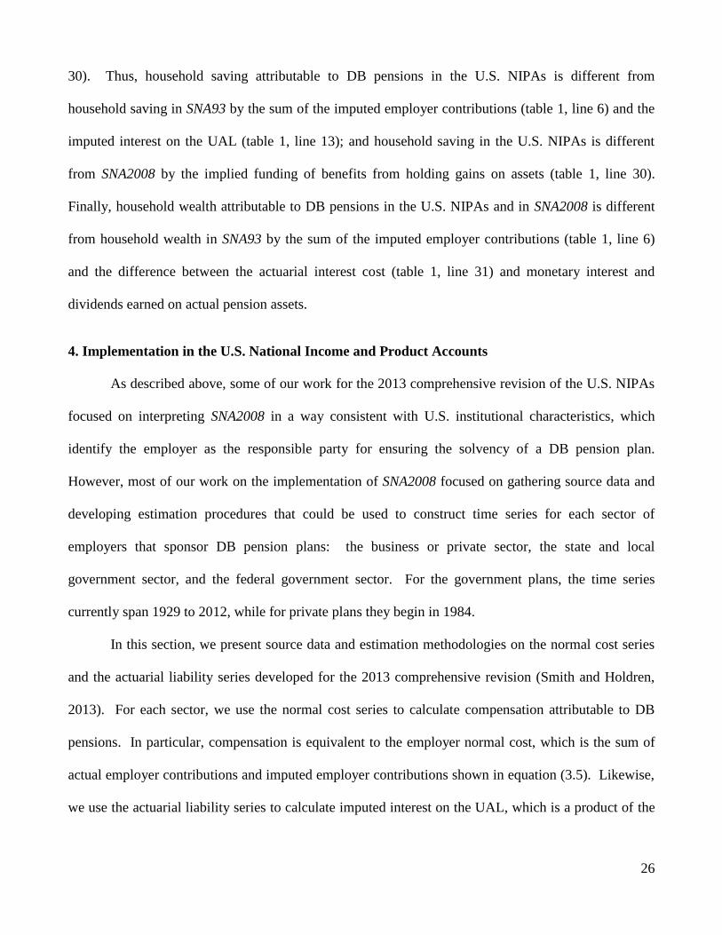
30). Thus, household saving attributable to DB pensions in the U.S. NIPAs is different from

household saving in SNA93 by the sum of the imputed employer contributions (table 1, line 6) and the

imputed interest on the UAL (table 1, line 13); and household saving in the U.S. NIPAs is different

from SNA2008 by the implied funding of benefits from holding gains on assets (table 1, line 30).

Finally, household wealth attributable to DB pensions in the U.S. NIPAs and in SNA2008 is different

from household wealth in SNA93 by the sum of the imputed employer contributions (table 1, line 6)

and the difference between the actuarial interest cost (table 1, line 31) and monetary interest and

dividends earned on actual pension assets.

4. Implementation in the U.S. National Income and Product Accounts

As described above, some of our work for the 2013 comprehensive revision of the U.S. NIPAs

focused on interpreting SNA2008 in a way consistent with U.S. institutional characteristics, which

identify the employer as the responsible party for ensuring the solvency of a DB pension plan.

However, most of our work on the implementation of SNA2008 focused on gathering source data and

developing estimation procedures that could be used to construct time series for each sector of

employers that sponsor DB pension plans: the business or private sector, the state and local

government sector, and the federal government sector. For the government plans, the time series

currently span 1929 to 2012, while for private plans they begin in 1984.

In this section, we present source data and estimation methodologies on the normal cost series

and the actuarial liability series developed for the 2013 comprehensive revision (Smith and Holdren,

2013). For each sector, we use the normal cost series to calculate compensation attributable to DB

pensions. In particular, compensation is equivalent to the employer normal cost, which is the sum of

actual employer contributions and imputed employer contributions shown in equation (3.5). Likewise,

we use the actuarial liability series to calculate imputed interest on the UAL, which is a product of the

27

discount rate and the difference between the actuarial liability and plan assets as shown in equation

(3.13).

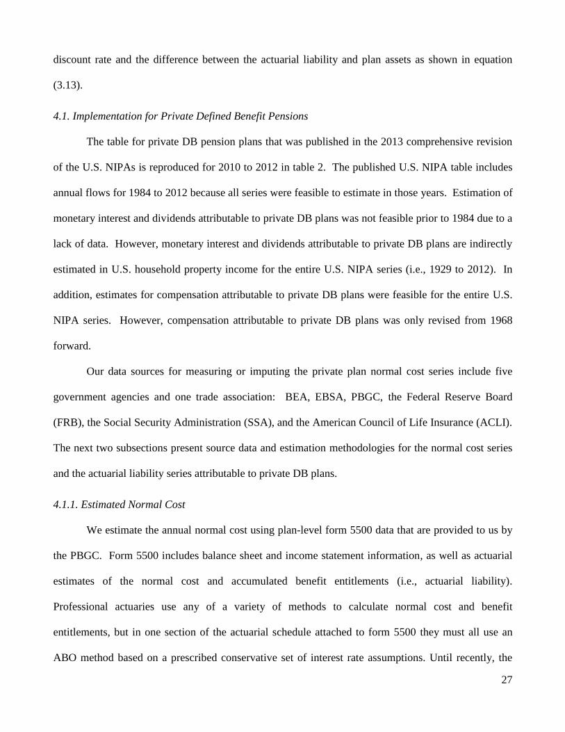
4.1. Implementation for Private Defined Benefit Pensions

The table for private DB pension plans that was published in the 2013 comprehensive revision

of the U.S. NIPAs is reproduced for 2010 to 2012 in table 2. The published U.S. NIPA table includes

annual flows for 1984 to 2012 because all series were feasible to estimate in those years. Estimation of

monetary interest and dividends attributable to private DB plans was not feasible prior to 1984 due to a

lack of data. However, monetary interest and dividends attributable to private DB plans are indirectly

estimated in U.S. household property income for the entire U.S. NIPA series (i.e., 1929 to 2012). In

addition, estimates for compensation attributable to private DB plans were feasible for the entire U.S.

NIPA series. However, compensation attributable to private DB plans was only revised from 1968

forward.

Our data sources for measuring or imputing the private plan normal cost series include five

government agencies and one trade association: BEA, EBSA, PBGC, the Federal Reserve Board

(FRB), the Social Security Administration (SSA), and the American Council of Life Insurance (ACLI).

The next two subsections present source data and estimation methodologies for the normal cost series

and the actuarial liability series attributable to private DB plans.

4.1.1. Estimated Normal Cost

We estimate the annual normal cost using plan-level form 5500 data that are provided to us by

the PBGC. Form 5500 includes balance sheet and income statement information, as well as actuarial

estimates of the normal cost and accumulated benefit entitlements (i.e., actuarial liability).

Professional actuaries use any of a variety of methods to calculate normal cost and benefit

entitlements, but in one section of the actuarial schedule attached to form 5500 they must all use an

ABO method based on a prescribed conservative set of interest rate assumptions. Until recently, the

28

ABO method required of all plans was referred to as the RPA ’94 method, because it was required by

the Retirement Protection Act of 1994. The reporting requirements are now governed by the Pension

Protection Act (PPA) of 2006, but the “funding target” and “target normal cost” concepts of the PPA

are similar to current liability and normal cost concepts used in RPA ’94.16

Because we adjust for

differences interest rate assumptions, the PPA variables can be treated as continuations of the RPA ’94

variables with no break in series.

For 2000 to 2011, we tabulate the RPA ’94 normal cost or target normal cost reported on form

5500. For 2000, 2001, and 2011, we make a coverage adjustment for plans that are missing from the

data set. Prior to 2000, we do not have form 5500 data. However, by assuming that future benefit

payments provide a good indicator of benefits accrued for current service, we can back-cast the rates to

1929 to 1999, using as an indicator the percentage change in the rate at which future benefits are paid.

We back-cast the normal cost rate rather than the normal cost level so that we can capture the effects of

variation in wages and salaries as well as variation in coverage rates. When possible, we use a 20-year

lag between benefits paid and normal cost.17

We also do not have form 5500 data for 2012 because the

data are only available with an 18-month lag. Thus, we extrapolate 2012 using the previous 2-year

average normal cost rate. We limit the average to two years because our assumed discount rate is the

same for 2010 to 2012.

We adjust all years to a discount rate based on AAA corporate bond rates published by the U.S.

FRB. Our adjustments for the interest rate assumption changes are based on standard formulas

provided by PBGC. The formulas apply different discounting for active participants and retirees and

are summarized in appendix A. We construct a discount rate series based on assumptions laid out in

16

One noteworthy difference is that the PPA uses short term interest rates to discount benefit expenses that fall due in the

short term, so the effective average interest rate assumption tends to be a bit lower than under the RPA ‘94. 17

The correlation coefficient between benefits paid and normal cost for 2000 to 2008 is 0.88. A regression of normal cost

on benefits paid for 2000 to 2008 yields an adjusted r-squared of 0.74 and a statistically significant positive coefficient

estimate. We are unable to use a 20-year lag for this analysis because data for benefits paid are not available 20 years into

the future. However, we perform the same analysis for liabilities with a lag, which yields even stronger results (adjusted r-

squared of 0.90 and a statistically significant positive coefficient estimate).

29

appendix B. The resulting U.S. NIPA discount rate series and the related AAA corporate bond rate

series are presented in appendix B in table B1. We use the same discount rate series for private plans

and state and local plans. The top four panels of appendix C table C1 summarize source data and

methodologies by year for the normal cost series of private DB plans.

4.1.2. Estimated Actuarial Liability

The procedure for estimating the annual actuarial liability requires two variables: the funding

ratio and plan assets. Since we do not initially have a complete time series for plan liabilities, we first

calculate funding ratios and then apply the ratios to plan assets to calculate a measure of plan

liabilities.

Funding Ratios: For 1979 to 2008, we calculate annual funding ratios using tabulations

published by PBGC of plan assets and plan liabilities reported on form 5500. Plan assets are reported

at market value. Plan liabilities are adjusted by PBGC to a common discount rate by year (i.e.,

discount rates vary across years but do not vary across plans within a year). For 1950 to 1978, we use

annual funding ratios published by Ippolito (1986). Ippolito (1986) calculates funding ratios based on

the market value of plan assets published by the FRB in the Flow of Funds Accounts (FFAs; since

renamed the Financial Accounts of the United States) and plan liabilities, which are determined by

applying annual aggregate data on number of participants and benefits paid published in Skolnik

(1976) to parameter estimates of the relationship between reported liabilities and reported discount

rates on form 5500 for 1978.18

We adjust liabilities for all years using the relevant rate from the U.S.

NIPA discount rate series. In addition to the estimated funding ratios for 1950 to 2008, we assume a

funding ratio of 15 percent for 1929, which is consistent with the funding ratio cited in Williamson

(1992) and Sass (1997) based on Latimer (1932) of approximately 13 to 16 percent.

18

Ippolito (1986) makes an adjustment to remove assets and liabilities related to DC plans.

30

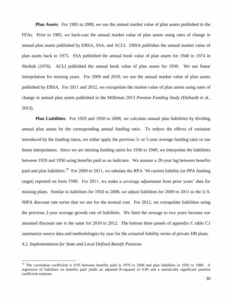
Plan Assets: For 1985 to 2008, we use the annual market value of plan assets published in the

FFAs. Prior to 1985, we back-cast the annual market value of plan assets using rates of change in

annual plan assets published by EBSA, SSA, and ACLI. EBSA publishes the annual market value of

plan assets back to 1975. SSA published the annual book value of plan assets for 1940 to 1974 in

Skolnik (1976). ACLI published the annual book value of plan assets for 1930. We use linear

interpolation for missing years. For 2009 and 2010, we use the annual market value of plan assets

published by EBSA. For 2011 and 2012, we extrapolate the market value of plan assets using rates of

change in annual plan assets published in the Milliman 2013 Pension Funding Study (Ehrhardt et al.,

2013).

Plan Liabilities: For 1929 and 1950 to 2008, we calculate annual plan liabilities by dividing

annual plan assets by the corresponding annual funding ratio. To reduce the effects of variation

introduced by the funding ratios, we either apply the previous 3- or 5-year average funding ratio or use

linear interpolation. Since we are missing funding ratios for 1930 to 1949, we interpolate the liabilities

between 1929 and 1950 using benefits paid as an indicator. We assume a 20-year lag between benefits

paid and plan liabilities.19

For 2009 to 2011, we tabulate the RPA ’94 current liability (or PPA funding

target) reported on form 5500. For 2011, we make a coverage adjustment from prior years’ data for

missing plans. Similar to liabilities for 1950 to 2008, we adjust liabilities for 2009 to 2011 to the U.S.

NIPA discount rate series that we use for the normal cost. For 2012, we extrapolate liabilities using

the previous 2-year average growth rate of liabilities. We limit the average to two years because our

assumed discount rate is the same for 2010 to 2012. The bottom three panels of appendix C table C1

summarize source data and methodologies by year for the actuarial liability series of private DB plans.

4.2. Implementation for State and Local Defined Benefit Pensions

19

The correlation coefficient is 0.95 between benefits paid in 1970 to 2008 and plan liabilities in 1950 to 1988. A

regression of liabilities on benefits paid yields an adjusted R-squared of 0.90 and a statistically significant positive

coefficient estimate.

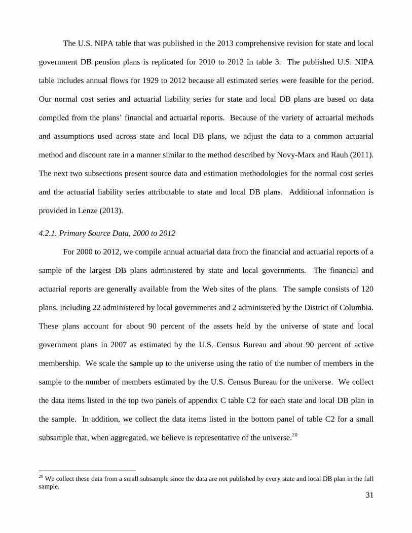
31

The U.S. NIPA table that was published in the 2013 comprehensive revision for state and local

government DB pension plans is replicated for 2010 to 2012 in table 3. The published U.S. NIPA

table includes annual flows for 1929 to 2012 because all estimated series were feasible for the period.

Our normal cost series and actuarial liability series for state and local DB plans are based on data

compiled from the plans’ financial and actuarial reports. Because of the variety of actuarial methods

and assumptions used across state and local DB plans, we adjust the data to a common actuarial

method and discount rate in a manner similar to the method described by Novy-Marx and Rauh (2011).

The next two subsections present source data and estimation methodologies for the normal cost series

and the actuarial liability series attributable to state and local DB plans. Additional information is

provided in Lenze (2013).

4.2.1. Primary Source Data, 2000 to 2012

For 2000 to 2012, we compile annual actuarial data from the financial and actuarial reports of a

sample of the largest DB plans administered by state and local governments. The financial and

actuarial reports are generally available from the Web sites of the plans. The sample consists of 120

plans, including 22 administered by local governments and 2 administered by the District of Columbia.

These plans account for about 90 percent of the assets held by the universe of state and local

government plans in 2007 as estimated by the U.S. Census Bureau and about 90 percent of active

membership. We scale the sample up to the universe using the ratio of the number of members in the

sample to the number of members estimated by the U.S. Census Bureau for the universe. We collect

the data items listed in the top two panels of appendix C table C2 for each state and local DB plan in

the sample. In addition, we collect the data items listed in the bottom panel of table C2 for a small

subsample that, when aggregated, we believe is representative of the universe.20

20

We collect these data from a small subsample since the data are not published by every state and local DB plan in the full

sample.

32

We separate the actuarial liability into (1) an active member liability and (2) a retired member

liability (i.e., the liability to all beneficiaries including disabled and survivor beneficiaries). Although

GASB does not require plans to publish separate liabilities, it is possible to obtain the active and retired

member liabilities for most pension plans. These data can often be obtained from a table called the

Solvency Test, which many pension plans publish in the actuarial section of their Comprehensive

Annual Financial Reports.

4.2.2. Estimated Normal Cost and Actuarial Liability

Given a few basic facts about a worker (such as age, years of service, and salary) and about the

pension plan (such as the salary multiplier and COLAs to retirement benefits), and using standard risk

factors (such as the mortality rates summarized in an annuity table), we can calculate the expected

stream of pension benefits. With the additional assumption of a discount rate, we can discount the

stream to a present value.

In order to standardize the actuarial liability estimates prepared by different DB plans using

different actuarial methods and different discount rates, we perform two sets of calculations. First, we

calculate the liability for a given plan using the plan’s preferred actuarial method and the plan’s

preferred discount rate. Second, we calculate the liability using an ABO method and the discount rate

chosen for the U.S. NIPAs. We then use the ratio of the two estimates to convert the liabilities of all

plans that used the plan’s preferred actuarial method and the plan’s preferred discount rate to the ABO

method and the U.S. NIPA discount rate.

Our liability estimate, calculated using the plan’s actuarial method and discount rate, will differ

from the estimate calculated by the plan because the plan has a richer information set on members and

the provisions of the plan and because the plan will use different assumptions. However, the

differences often have very similar effects on the liabilities calculated by the different actuarial

methods and hence have a negligible effect on their ratio. For example, the liability calculated using a

33

mortality table for males will be different from a liability using a mortality table for females because of

the longer expected lifespan of females. However, the ratio of the ABO liability to the plan’s liability

calculated using the male mortality table will be almost identical to the ratio calculated using the

female mortality table.

The procedure for standardizing the normal cost and the actuarial liability for active members is

summarized in six steps. First, we specify the provisions of a typical pension plan shown in appendix

C, table C3, and the provisions are held constant over time. Second, we select a set of economic and

actuarial assumptions also shown in appendix C, table C3.21

Third, we estimate the normal cost and

the liability for workers of various ages and years of service using the equations in Winklevoss (1993)

for ABO and PBO actuarial methods.22

We calculate weighted averages of the estimates using the

actual distribution of active members by age and years of service as weights. The actual distribution of

active members is based on data collected annually. Fourth, we construct ratios of the weighted

averages as calculated under each actuarial method—the ratios vary annually. Fifth, we multiply the

published normal cost and liability for an individual state and local plan by the relevant ratio to convert

the normal cost and liability to an equivalent based on the ABO method and the discount rate chosen

for the U.S. NIPAs. Finally, we subtract actual member contributions as published by the plan in its

financial statements from the ABO estimate of normal cost to obtain the employer normal cost.

An example of the normal cost for workers of various ages and years of service, calculated

using provisions of the typical pension plan, an 8.0 percent discount rate, and the entry age actuarial

21

Most of the assumptions are held constant over time. However, as indicated in appendix B table B1, the discount rate

assumptions used for U.S. NIPA estimates change over time. Since the real interest rate is held constant at 2.5 percent,

expected inflation falls when the discount rate falls. Since wage growth depends on expected inflation, wage growth also

falls. Although we know the discount rates used by individual state and local DB plans in their actuarial calculations, we

do not know their inflation rates. Therefore, we assume that individual plans use a real rate of approximately 4.5 percent.

Whenever plans change their discount rate, they lower the inflation component, leaving the real rate unchanged. For a

retirement system using an 8 percent discount rate, this assumption implies an inflation rate of 3.5 percent. See the

distribution of inflation rate assumptions in Brainard (2011). 22

The PBO methods include the entry age method and the projected unit credit method. The equations we use are

discussed on pp.118-122 of Winklevoss (1993). In particular, we use equation 8.7 for the ABO method, equation 8.8 for

the constant dollar projected unit credit method, and the constant percent versions of equations 8.10a and 8.10b for the

entry age method.

34

method (i.e., a PBO method) is presented in panel A of appendix C table C4. Normal cost calculated

for the same plan but using a 5.5 percent discount rate and the ABO method (all other assumptions the

same as before) are presented in panel B. The actual distribution of active members by age and years

of service is presented in panel C. Using the data in panel C as weights, the average ABO normal cost

is $6,375 per worker, the average entry age normal cost is $2,927, and their ratio is 2.2. Thus, to

convert the published normal cost of a state and local DB plan that uses the entry age method and an

8.0 percent discount rate to our ABO, 5.5 percent standard, we would multiply it by 2.2.

Since the retired member liability is the same for all actuarial methods it needs only a discount

rate adjustment. Using the source data listed in appendix C table C2 and the plan provisions and

assumptions listed in table C3, we calculate the present value of expected benefits per retiree for a set

of retirees of different ages. We multiply the estimates by the number of retirees in each of the age

intervals and sum to obtain an aggregate retired member liability for the typical pension plan. We

perform the calculations using the discount rates used by the individual pension plans in our sample

and using the discount rates chosen for the U.S. NIPAs. We then calculate a set of adjustment factors

as the ratio of the retired member liability of the typical pension plan based on the U.S. NIPA discount

rate to the liability based on the sample discount rate. Finally, we multiply the published retired

member liabilities of the pension plans in our sample by the relevant adjustment factor to standardize

them to the U.S. NIPA discount rate.

Before 2000, a simpler methodology was used for three reasons: 1) little actuarial data was

readily available for making the estimates, 2) many pension plans, including some of the largest plans

used the so-called aggregate method, which generates a meaningless liability measure for national

income accounting purposes, and 3) financial accounting standards for state and local government

pension plans were in an unsettled state until GASB adopted Statement No. 25 in November 1994 and

made it effective for financial statements for fiscal years beginning after June 15, 1996.

35

Instead of using plan-level data, we calculate a normal cost per active employee, a liability per

active employee, and a liability per beneficiary for representative employees and beneficiaries

participating in a representative pension plan and then multiply the per person amounts by the number

of active employees and the number of beneficiaries to generate a time series of aggregate normal cost

and aggregate liabilities. We have annual estimates back to 1929 of employees and beneficiaries based

on surveys from the U.S. Census Bureau and other agencies. We characterize representative agents

and plans based on a wide variety of data sources for various dates from 1929 to 2000.

4.3. Implementation for Federal Defined Benefit Pension Plans

The estimates of normal cost and interest cost for the federal government DB plans are based

on simulations calibrated to match the normal cost, actuarial liability and benefit expense information

in the annual reports for CSRS, FERS, and the military plan. In the simulations, the sum of the

employer and employee contributions is set equal to normal cost, where normal cost is calculated as

the reported or inferred normal cost rate times the total pay of the employees covered by the plan. The

income that the plan gets from its assets is calculated using the rate of interest assumed in the actuarial

calculations of the normal cost rate. The initial level of assets and the two adjustments to assets were

calibrated so that the simulated assets in 2013 (military plan) or 2014 (civilian plans) equaled the

published estimate of the actuarial liability in that year.23

Starting in any year t, assets in year t+1 were

solved for by the equation:

(4.1) Assets in period t+1 = Assets in period t + contributions + interest income from plan assets –

benefits and administrative expenses + adjustment for inflation or interest rate regime shift.

Equation (4.1) is the same as equation (2.1) above except for the term that adjusts for regime

shifts. In the simulations, just two such adjustments were included, one in 1970, when there was an

23

Estimates of actuarial liabilities are based on projections, so predicting what the actuarial liability will be on a future date

is not so different from estimating its value as of today. Projections of future year actuarial liabilities are published in the

annual reports for the federal plans.

36

upward shift in the inflation regime, and another in 2010, when there was a downward shift in the

interest rate without a corresponding change in the inflation rate. Since contributions always equal the

normal cost and the assets earn the rate of interest used to calculate the normal cost, the value of the

accumulated plan assets at the end of a year can be assumed to equal the actuarial liability at that point

in time. (To estimate interest income from assets more precisely, intra-year variation in plan assets

should be taken into account in fitting equation (4.1).)

The interest rate assumptions are based on the rates assumed by the actuaries in preparing the

annual reports, supplemented by information on Treasury bond yields for the years before the reports

began. However, a cut in the interest rate assumption that was implemented in the reports starting in

2012 was started two years earlier in the simulations. The history of the interest rate assumptions in the

federal plan simulations is shown in appendix B, table B2. Except for in 2010, whenever the interest

rate assumption was changed, the inflation rate and salary growth rate assumptions were assumed to

change too, so that the real rate of interest was unaffected. With the real rate of interest held constant,

the effect on the PBO actuarial liability was small enough to be ignored. (Federal plan benefit

expenses are sensitive to inflation because inflation raises the average salary in the last three years of

the career, which is used to set the initial benefit level, and because during retirement benefits are

escalated by the change in the consumer price index (CPI), or CPI minus 1 percent in the case of

FERS.)

Table 4 replicates the 2010 to 2012 columns of the table for federal government DB pension

plans that was published in the 2013 comprehensive revision of the U.S. NIPAs (the published U.S.

NIPA table goes back to 1929). The annual reports are on a federal fiscal year basis (October to

September ever since 1976), so we convert estimates to a calendar year by dividing by four and adding

the calendar quarters. The next two subsections present source data and estimation methodologies for

the normal cost series and the actuarial liability series attributable to federal DB plans.

37

4.3.1. Estimated Normal Cost

We estimate the annual normal cost for federal civilian plans based on plan-level data from

annual reports issued by the U.S. Office of Personnel Management (OPM). Likewise, we estimate the

annual normal cost for federal military plans based on plan-level data from annual reports issued by

OPM and the U.S. Department of Defense (DOD).

The normal cost is available in annual reports from 1987 to 2012 for CSRS, which started in

1920, and was funded on a pay-as-you-go basis until 1969, when the U.S. government started making

catch-up contributions to the plan. Annual reports are available from 1984 to 2012 for FERS, which

effectively started in 1984 and has been funded through contributions since inception. In addition to

CSRS and FERS, we make a coverage adjustment for much smaller civilian plans that do not make

annual reports readily available. The coverage adjustment is 2.8 percent of CSRS and FERS

combined.24

Annual reports are available from 1985 to 2012 for the large military plan that was on a

pay-as-you-go basis from 1936 to 1984. We make a coverage adjustment to the large military plan to

account for a small plan sponsored by the U.S. Coast Guard, which operates on a pay-as-you-go basis.

Prior to 1979 for civilian plans and prior to 1985 for military plans, we do not have source data

on the normal cost. We back-cast the rate by adjusting for significant changes in federal plan

provisions and the inflation environment. For CSRS, the 1979 normal cost rate was used for the high

inflation years of 1971 to 1979, but the rate from the more normal inflation regime of 1987 was used in

1970. Going backwards in time, the assumed 1970 normal cost rate was adjusted down in 1969, 1956

and 1942 to reflect the lower generosity of the rules in effect before those dates.25

For the years up to

1989 in the military plan simulation, the normal cost rate was assumed to be 47 percent of pay, which

24

The objective of the coverage adjustment is to include plans sponsored by the U.S. Department of State for foreign

service, the Tennessee Valley Authority, the U.S. judicial and legislative branches of government, and the FRB. 25

For the civilian plans, there were changes in key factors in 1930, 1942, 1948, 1956, and 1969. Key factors for the years

include the addition of survivors’ benefits and changes in the benefit formula. For the military plan, we adjust the normal

cost rate from 1985 to 1989 but we otherwise hold the normal cost rate constant. In addition, we include upward

adjustments for the civilian plans and the military plan in 1970 for the inflation surprise and in 2009 and 2010 for the

interest rate decline that was not matched by an inflation decline. We do not adjust for changes in mortality rates over time.

38

is slightly below the normal cost rates in 1985 to 1989 published by the Department of Defense

actuaries. However in 1943 to 1946, the normal cost in dollars was held down at its 1942 level

because a large share of military personnel in 1943 to 1946 did not stay in for long enough to get a

pension. The top panel of appendix C table C5 summarizes source data and methodologies by year for

the normal cost series of federal DB plans.

4.3.2. Estimated Actuarial Liability

Values of the actuarial liability are needed to estimate the interest cost component of the

income that households receive from participation in DB pension plans. Estimates of the actuarial

liability of the main federal plans are available in their annual reports. Yet these estimates do not

extend back into early periods and they can change in an erratic way from one year to the next or

because of experience gains and losses or assumption changes. Also, in some periods of time, the

experience gains and losses tend to be consistently in one direction, which implies that at least on an ex

post basis, there is a bias in the projections that underlie the calculation of the actuarial liability. We

therefore use the published values of the actuarial liability in 2013 or 2014 as benchmarks for setting

the level of the actuarial liability profile over time and use the published values for other years as

indicators of the slope and curvature of this profile. In practice, this means that the goals of the

simulation of the evolution of the plan assets are to hit the end year actuarial liability exactly and to

approximate a smoothed version of the profile of the actuarial liabilities for other years. The simulated

assets as of the beginning of the year are used to estimate the actuarial liability at that time. Of course,

the plan assets change every month as benefits are paid and contributions are received, so the interest

cost was calculated as the interest rate times the opening value of the assets plus 11/24 times the

interest rate times the normal cost during the plan year minus 13/24 times the interest rate times the

benefits paid during the plan year. The factors of 11/24 and 13/24 reflect the fact that the normal costs

are paid at the end of the month, while benefits are paid at the beginning of the month.

39

To verify the robustness and accuracy of the simulations, we also attempted to model the long

run future evolution of the pension plan assets. In the case of CSRS, which has long been closed to

new participants, the estimation objective was to have the trust fund balance hit zero at the time of

death of the last survivor drawing benefits. In the case of FERS and the military plan, which do not

have finite lives, the objective was long run stability of the simulated ratio of assets to benefits. We

were able to achieve this objective in the simulations for the military plan.

For FERS, the actuarial liability is zero in 1984, but the actuarial liability for CSRS and the

military plan are greater than zero in 1929—the first year of our time series. We use our annual

normal cost estimates to estimate the annual actuarial liability assuming the annual change in actuarial

liability is the same as the change in the assets in equation (4.1). We have complete time series from

the U.S. NIPAs on covered payroll and benefit payments to use as inputs into the simulations. We use

the estimates of actuarial liability to infer payments of interest on plans assets. Finally, plan rules that

affect the normal cost estimates are incorporated in the actuarial liability via the normal cost

component of the change in actuarial liability. However, we adjust the actuarial liability of plans

upward in 1970 for the inflation surprise and in 2009 and 2010 for the interest rate decline that was not

matched by an inflation decline. The bottom panel of appendix C table C5 summarizes source data

and methodologies by year for the actuarial liability series of federal DB plans.

5. Effects of Defined Benefit Pensions in the U.S. National Income and Product Accounts

To show the effects of the new treatment of DB pension plans in the U.S. NIPAs, we present

transactions of DB pension plans for the 3-year period 2010 to 2012 as shown in the U.S. NIPAs. We

also compare accrual measures and cash measures of U.S. household income, saving, and change in

wealth attributable to DB pension plans for the 10-year period 2003 to 2012.

5.1. Transactions of Defined Benefit Pension Plans

40

DB pension transactions from the U.S. NIPAs are presented in tables 2, 3, and 4 for plans

sponsored by private business, state and local governments, and the federal government, respectively.

In addition, table 5 presents transactions for plans sponsored by employers in all three sectors. We

focus our discussion on the following series in each table: 1) imputed employer contributions, 2)

actual household contributions, 3) pension service charges, 4) imputed interest on the UAL, 5)

household income, 6) household saving, and 7) changes in household wealth.

Imputed employer contributions are shown on line 6 of each table. In recent years, imputed

employer contributions have generally been negative for private plans because private employers were

making catch-up contributions to close funding gaps resulting from the bursting of the dot-com stock

market bubble and the financial crisis. Imputed employer contributions for federal plans are positive

through 1979 but negative thereafter. Imputed employer contributions for state and local plans are

positive each year 1929 to 2012 with the exception of a few years in the early 1980s. The positive

estimates reflect persistently inadequate actual employer contributions, while the negative ones reflect

extra contributions that mostly covered the interest accruing on the UAL that had arisen during the

years of inadequate contributions.

Actual household contributions and pension service charges are presented on lines 7 and 8,

respectively. Actual household contributions reflect contributions required of employees and are

relatively small for private plans and federal plans, but large for state and local plans. In recent years,

employees have been required to contribute approximately 20 percent of the annual benefit

entitlements earned through service to state and local government employers. In contrast, employees

in private and federal plans contribute approximately 1 percent and 5 percent of annual benefit

entitlements earned, respectively. For all plans, pension service charges are low relative to assets;

however, pension service charges are much higher for private plans and state and local plans than for

federal plans.

41

Imputed interest on the UAL is shown in each table on line 13. Imputed interest on the UAL is

generally positive for all plans, reflecting persistent underfunding. Values in the series for private

plans tend to be relatively small in magnitude, however, because of regulatory funding requirements

for these plans. Values in the series for state and local plans are relatively large after the losses of the

financial crisis, but are small prior to 2009. Values in the series for federal plans are relatively large

over most of the time series, reflecting the federal government’s funding of benefit payments as they

come due.

The effects of DB pensions on U.S. household income, saving, and wealth are reported in each

table on lines 27, 29, and 33, respectively. Based on the new accrual approach, state and local

government plans have been the largest contributor to household income, saving and wealth since the

early 1990s. However, prior to the 1990s, private DB plans contributed more to each measure than the

state and local plans, and federal plans contributed more to each measure than private plans and state

and local plans.

5.2. Comparisons of Accrual and Cash Measures

To facilitate comparisons between the accrual and cash measures of pension plans, tables 6, 7,

8, and 9 present accrual measures of household income, saving, and change in wealth attributable to

DB pensions plans as a percentage of household disposable income followed by cash measures of

household income, saving, and change in wealth. Tables 6, 7, and 8 present plans sponsored by private

business, state and local governments, and the federal government, respectively; table 9 combines the

plans sponsored by employers in all three sectors.

In the tables, household income is broken down into compensation and property income

components. The difference between accrual and cash measures of household income comes from the

imputed elements of these two components, and this difference is in fact equal to the sum of the

imputed employer contributions and the imputed interest paid by the employer on the UAL. In

42

addition, the tables show the contribution of implied funding from holding gains to the accrual measure

of the change in household wealth. The cash measure of change in wealth uses actual holding gains.

State and local government plans generate more income for U.S. households than private plans

or federal plans in the period 2003 to 2012, and compared with private plans, they are more important

both in terms of compensation income and property income. However, household property income

from federal plans is higher than from state and local government plans in recent years because of the

large amounts of imputed interest on the UAL of the federal plans. The higher household income

attributable to state and local plans also yields higher household saving and a higher change in

household wealth attributable to state and local plans over the period.

Although the household income and saving attributable to federal plans is higher than the

income and saving attributable to private plans over all the years shown in tables 6 through 9, the

change in household wealth is consistently higher for private plans than for federal plans because

implied funding from holding gains attributable to federal plans is always zero—the plans do not hold

equities.

For the years shown, accrual measures of household compensation attributable to private plans

in table 6 and federal plans in table 8 are generally lower than cash measures because actual employer

contributions are offset by negative imputed employer contributions caused by employers making

catch-up contributions. In the case of private plans, accrual measures of household property income

are generally close to cash measures because imputed interest on the UAL is relatively low. Thus,

accrual based household income attributable to private plans is generally lower than cash based

household income for the period. In the case of federal plans, accrual measures of household property

income are consistently higher than cash measures because imputed interest on the UAL is almost 1

percent of household disposable income. The difference in property income offsets the difference in

43

compensation income. Thus, accrual based household income attributable to federal plans is generally

higher than cash based household income for the period.

In contrast to private plans and federal plans, the state and local government plans have higher

accrual measures of household compensation than cash measures for the entire period shown in table 7

because actual employer contributions are not enough to cover benefit entitlements earned on each

year’s labor services. In addition, imputed interest on the UAL is consistently positive for state and

local plans during the period because the plans are underfunded in the period shown.

Accrual based household income presented in table 9 for all plans combined is also higher than

cash based household income for all years shown. While accrual based household compensation

attributable to all plans is not higher than cash based household compensation for some years, imputed

interest on the UAL due to underfunding of federal plans and state and local plans is more than enough

to offset the differences in household compensation income for each year. Thus, for the period 2003 to

2012, accrual measures of household income are higher than cash measures by amounts in the range of

1 to 2 percent of household disposable income.

The effects of accrual based measurement on household saving are the same as on household

income. In particular, accrual based household saving attributable to private plans is tends to be

slightly lower than cash based household saving, though the difference in average levels is small, at a

mere 0.1 percent of household disposable income. In contrast, accrual measures of household saving

attributable to state and local government plans and federal plans are consistently higher than the cash

measures. When all plans are combined, the differences attributable to private plans are more than

offset by the differences attributable to the government plans. Thus, for the period 2003 to 2012,

accrual measures of household saving attributable to DB pensions are also 1 to 2 percentage points

higher than cash measures as a percentage of household disposable income.

44

In SNA93, household wealth includes assets held by pension plans, so the cash based change in

household wealth attributable to DB pension plans is calculated by subtracting the market value of plan

assets at the beginning of the period from the market value of plan assets at the end of the period.

Because of the volatility of market values of equity assets held by private plans and by state and local

government plans, the cash based change in household wealth attributable to private plans and state

and local plans tends to be more volatile than the accrual measures. For example, the cash based

change in household wealth attributable to private plans and state and local government plans dips in

2008 in response to the financial crisis. In contrast, the cash based change in wealth attributable to

federal plans is smooth because federal plans do not invest in equities.

In the U.S. NIPAs, the accrual measure of the change in household wealth attributable to DB

pension plans includes the implied funding of benefits from holding gains to accrual based household

saving. The implied funding from holding gains is a residual between the interest that the actual plan

assets would generate if they all earned the interest rate assumed in the actuarial calculations and the

property income actually earned on those assets. (Alternatively, if the interest from the employer on

the UAL is included with the other property income, the implied holding gains equal the difference

between the plan’s property income and the interest cost of the actuarial liability.) If over the long-run

the total return on plan assets is equal to the assumed rate of interest and the return consists of holding

gains plus property income from interest and dividends, the gap between the assumed rate of interest

and property income yield on the plan assets is the part of the return that is implicitly assumed to come

from holding gains.

Differences between accrual measures and cash measures of the change in household wealth

tend to be driven by volatility in the market value of equity assets held by pension plans. For the

period 2003 to 2012, accrual measures of household wealth attributable to DB pensions are generally

higher than cash measures as a percentage of household disposable income. The cash measure of

45

change in wealth is probably held down by a combination of underfunding and poor stock market

returns.

6. Summary

With the 2013 comprehensive revision of the U.S. NIPAs, BEA replaced cash measures of the

transactions of defined benefit pension plans with accrual measures that use actuarial estimates of

benefit entitlements. Accrual measures of DB pension income are designed to match income earned

with the related production. In addition to this more meaningful way of measuring household income

and employer expenses related to pension plans, BEA introduced a new DB pension subsector and

showed a complete picture of its transactions in a new set of tables.

This paper provides a comprehensive summary of the U.S. experience with the new accrual

accounting treatment. The paper outlines DB pension concepts, available actuarial methods, and

relevant U.S. institutional characteristics and then explains how the concepts and methods were

applied in developing the specific measures for the U.S. NIPAs. In particular, it explains an

interpretation of SNA2008’s conceptual objectives that resulted in an additional property income flow

being recorded in the U.S. NIPAs. In addition, it presents the source data and estimation

methodologies that BEA uses to construct time series for each sector of U.S. employers that sponsor

DB pension plans. Finally, it presents results from the 2013 comprehensive revision that show how the

adoption of accrual based measurement of DB pension plans affected measures of household income,

saving, and wealth and of employers’ pension expenses. In particular, the household saving is higher

by between 1 and 2 percent of household disposable income when pensions are measured on an accrual

basis, and the pension expenses of state and local governments are also higher by between 1 and 2

percent of household disposable income.

46

References

Applebaum, Joseph. 1992. “Methods, and Funded Status of Defined Benefit Pension Plans” in Trends

in Pensions 1992. John A. Turner and Daniel J. Beller, eds. U.S. Department of Labor,

Pension and Welfare Benefits Administration: Washington, DC, pp. 509-529.

Brainard, Keith. 2006. Public Fund Survey Summary of Findings for FY 2005. National Association

of State Retirement Administrators.

Brainard, Keith. 2011. Public Fund Survey Summary of Findings for FY 2010. National Association

of State Retirement Administrators.

Brown, Jeffrey R. and David W. Wilcox. 2009. “Discounting State and Local Pension Liabilities.”

American Economic Review: Papers and Proceedings, 99(2), pp. 538-542.

Durant, Dominique, David Lenze, and Marshall Reinsdorf. 2010. “Adding Actuarial Information on

Defined Benefit Pension Plans and Social Security to the National Accounts.” Banque de

France and Bureau of Economic Analysis paper prepared for the CRIW/NBER conference on

Wealth, Financial Intermediation, and the Real Economy.

Ehrhardt, John W., Alan Perry, and Zorast Wadia. 2013. “2013 Pension Funding Study.” Milliman.

Falk, Justin. 2012. “Comparing Benefits and Total Compensation in the Federal Government and the

Private Sector.” Congressional Budget Office Working Paper Series 2012-4.

Gold, Jeremy and Gordon Latter. 2008. “The Case for Marking Public Plan Liabilities to Market.”

Pension Research Council Working Paper WP2008-20.

Ippolito, Richard A. 1986. Pensions, Economics and Public Policy. Pension Research Council. Dow

Jones-Irwin: Homewood, IL.

Kornfeld, Robert. 2013. “Initial Results of the 2013 Comprehensive Revision of the National Income

and Product Accounts.” Survey of Current Business, 93(8), pp. 6-17.

Latimer, Murray W. 1932. Industrial Pension Systems in the United States and Canada. Industrial

Relations Counselors, Inc.: New York.

Lazear, Edward P. and Robert L. Moore. 1988. “Pensions and Turnover” in Pensions in the U.S.

Economy, Z. Bodie, J. Shoven, and D. Wise (eds.), Chicago, IL: The University of Chicago

Press, pp. 163-188.

Lenze, David G. 2013. “State and Local Government Defined Benefit Pension Plans: Estimates of

Liabilities and Employer Normal Costs by State, 2000-2011.” BEA working paper WP2013-

16.

Moody’s Investors Service. 2013. Cross Sector Rating Methodology: Adjustments to US State and

Local Government Reported Pension Data, April 17.

47

Novy-Marx, Robert and Joshua D. Rauh. 2011. “Public Pension Liabilities: How big are they and

what are they worth?” Journal of Finance, 66(4), pp. 1207-1246.

Reinsdorf, Marshall B. and David G. Lenze. 2009. “Defined Benefit Pensions and Household Income

and Wealth.” Survey of Current Business, 89(8), pp. 50-62.

Sass, Steven A. 1997. The Promise of Private Pensions: The First Hundred Years. Pension Research

Council. Harvard University Press: Cambridge and London.

Shiller, Robert J. 2005. Irrational Exuberance. Princeton University Press: Princeton, NJ.

Skolnik, Alfred M. 1976. “Private Pension Plans, 1950-74.” Social Security Bulletin vol. 39, pp. 3-

17.

Smith, Shelly and Alyssa E. Holdren. 2013. “Preview of the 2013 Comprehensive Revision of the

National Income and Product Accounts.” Survey of Current Business, 92(3), pp. 13-39.

Stock, James H. and David A. Wise. 1990. “Pensions, the Option Value of Work, and Retirement.”

Econometrica, 58(5), pp. 1151-1180.

Wilcox, David W. 2006. “Reforming the Defined-Benefit Pension System.” Brookings Papers on

Economic Activity, 1 (Spring), pp. 235-304.

Williamson, Samuel H. 1992. “U.S. and Canadian Pensions before 1930: A Historical Perspective”

in Trends in Pensions 1992. Eds. John A. Turner and Daniel J. Beller, U.S. Department of

Labor, Pension and Welfare Benefits Administration: Washington, DC, pp. 35-57.

Winklevoss, Howard E. 1993. Pension Mathematics with Numerical Illustrations, 2nd

Edition.

University of Pennsylvania Press: Philadelphia, PA.

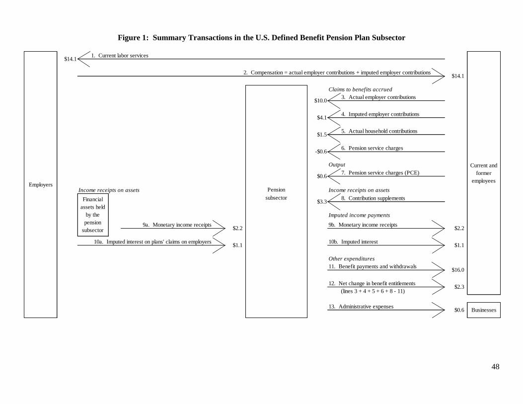
48

Figure 1: Summary Transactions in the U.S. Defined Benefit Pension Plan Subsector

Pension

subsector

$1.1 $1.1

Imputed income payments

Output

7. Pension service charges (PCE)

13. Administrative expenses$0.6 Businesses

Employers

$14.11. Current labor services

Current and

former

employees

2. Compensation = actual employer contributions + imputed employer contributions$14.1

Claims to benefits accrued

$10.03. Actual employer contributions

$4.1

Income receipts on assets Income receipts on assets

4. Imputed employer contributions

$1.55. Actual household contributions

-$0.66. Pension service charges

$0.6

10a. Imputed interest on plans' claims on employers 10b. Imputed interest

Financial

assets held

by the

pension

subsector

$3.38. Contribution supplements

9a. Monetary income receipts$2.2

12. Net change in benefit entitlements$2.3

(lines 3 + 4 + 5 + 6 + 8 - 11)

9b. Monetary income receipts$2.2

Other expenditures

11. Benefit payments and withdrawals$16.0

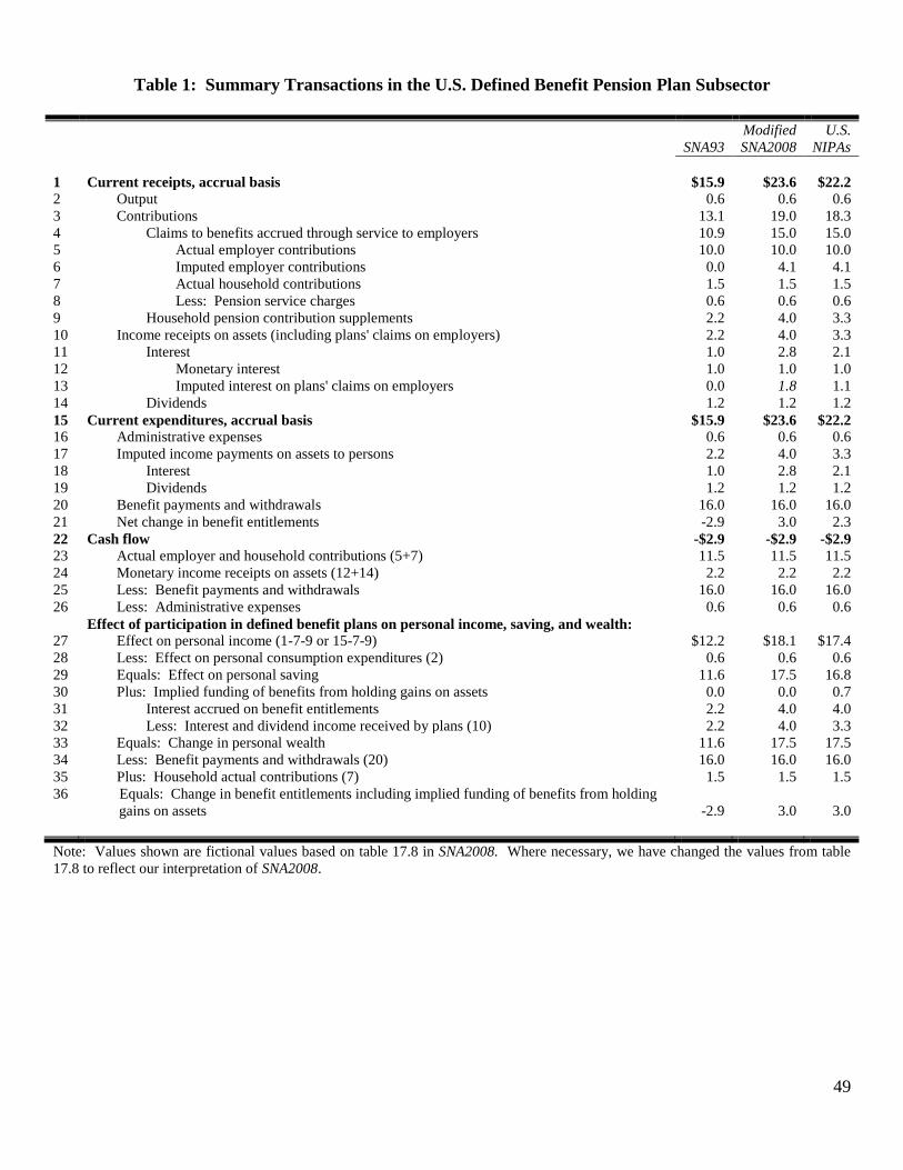
49

Table 1: Summary Transactions in the U.S. Defined Benefit Pension Plan Subsector

SNA93

Modified

SNA2008

U.S.

NIPAs

1 Current receipts, accrual basis $15.9 $23.6 $22.2

2 Output 0.6 0.6 0.6

3 Contributions 13.1 19.0 18.3

4 Claims to benefits accrued through service to employers 10.9 15.0 15.0

5 Actual employer contributions 10.0 10.0 10.0

6 Imputed employer contributions 0.0 4.1 4.1

7 Actual household contributions 1.5 1.5 1.5

8 Less: Pension service charges 0.6 0.6 0.6

9 Household pension contribution supplements 2.2 4.0 3.3

10 Income receipts on assets (including plans' claims on employers) 2.2 4.0 3.3

11 Interest 1.0 2.8 2.1

12 Monetary interest 1.0 1.0 1.0

13 Imputed interest on plans' claims on employers 0.0 1.8 1.1

14 Dividends 1.2 1.2 1.2

15 Current expenditures, accrual basis $15.9 $23.6 $22.2

16 Administrative expenses 0.6 0.6 0.6

17 Imputed income payments on assets to persons 2.2 4.0 3.3

18 Interest 1.0 2.8 2.1

19 Dividends 1.2 1.2 1.2

20 Benefit payments and withdrawals 16.0 16.0 16.0

21 Net change in benefit entitlements -2.9 3.0 2.3

22 Cash flow -$2.9 -$2.9 -$2.9

23 Actual employer and household contributions (5+7) 11.5 11.5 11.5

24 Monetary income receipts on assets (12+14) 2.2 2.2 2.2

25 Less: Benefit payments and withdrawals 16.0 16.0 16.0

26 Less: Administrative expenses 0.6 0.6 0.6

Effect of participation in defined benefit plans on personal income, saving, and wealth: 27 Effect on personal income (1-7-9 or 15-7-9) $12.2 $18.1 $17.4

28 Less: Effect on personal consumption expenditures (2) 0.6 0.6 0.6

29 Equals: Effect on personal saving 11.6 17.5 16.8

30 Plus: Implied funding of benefits from holding gains on assets 0.0 0.0 0.7

31 Interest accrued on benefit entitlements 2.2 4.0 4.0

32 Less: Interest and dividend income received by plans (10) 2.2 4.0 3.3

33 Equals: Change in personal wealth 11.6 17.5 17.5

34 Less: Benefit payments and withdrawals (20) 16.0 16.0 16.0

35 Plus: Household actual contributions (7) 1.5 1.5 1.5

36 Equals: Change in benefit entitlements including implied funding of benefits from holding

gains on assets -2.9 3.0 3.0

Note: Values shown are fictional values based on table 17.8 in SNA2008. Where necessary, we have changed the values from table

17.8 to reflect our interpretation of SNA2008.

50

Table 2: Transactions of Private Defined Benefit Pension Plans in the U.S. NIPAs

2010 2011 2012

1 Current receipts, accrual basis 277.1 270.5 268.1

2 Output /1/ 9.8 9.9 10.1

3 Contributions 173.4 168.6 167.2

4 Claims to benefits accrued through service to employers 79.4 76.6 76.4

5 Actual employer contributions 127.4 132.9 148.0

6 Imputed employer contributions -39.0 -47.3 -62.4

7 Actual household contributions 0.8 0.9 1.0

8 Less: Pension service charges /1/ 9.8 9.9 10.1

9 Household pension contribution supplements /2/ 94.0 92.0 90.8

10 Income receipts on assets (including plans' claims on employers) 94.0 92.0 90.8

11 Interest 66.2 65.6 61.8

12 Monetary interest 42.1 41.3 39.6

13 Imputed interest on plans' claims on employers /3/ 24.1 24.3 22.2

14 Dividends 27.8 26.4 29.0

15 Current expenditures, accrual basis 277.1 270.5 268.1

16 Administrative expenses 9.8 9.9 10.1

17 Imputed income payments on assets to persons 94.0 92.0 90.8

18 Interest 66.2 65.6 61.8

19 Dividends 27.8 26.4 29.0

20 Benefit payments and withdrawals 169.6 173.4 178.4

21 Net change in benefit entitlements /4/ 3.7 -4.8 -11.2

22 Cash flow 18.6 18.1 29.0

23 Actual employer and household contributions (5+7) 128.2 133.8 148.9

24 Monetary income receipts on assets (12+14) 69.8 67.7 68.6

25 Less: Benefit payments and withdrawals 169.6 173.4 178.4

26 Less: Administrative expenses 9.8 9.9 10.1

Effect of participation in defined benefit plans on personal income, saving, and wealth: 27 Effect on personal income (1-7-9 or 15-7-9) 182.4 177.7 176.3

28 Less: Effect on personal consumption expenditures (2) 9.8 9.9 10.1

29 Equals: Effect on personal saving 172.6 167.7 166.2

30 Plus: Implied funding of benefits from holding gains on assets 49.6 55.7 61.9

31 Interest accrued on benefit entitlements 143.6 147.7 152.7

32 Less: Interest and dividend income received by plans (10) 94.0 92.0 90.8

33 Equals: Change in personal wealth /5/ 222.3 223.4 228.1

34 Less: Benefit payments and withdrawals (20) 169.6 173.4 178.4

35 Plus: Household actual contributions (7) 0.8 0.9 1.0

36 Equals: Change in benefit entitlements including implied funding of benefits from holding

gains on assets /5/ 53.4 50.8 50.7

Legend / Footnotes:

1. Included in personal consumption expenditures as part of financial services furnished without payment; the value is equal to

administrative expenses (line 16).

2. Imputed income payments received by persons from the pension plans (line 17) are reinvested as household pension contribution

supplements.

3. Plans' claim on employers is the difference between actuarial liabilities and financial assets held by plans. When actuarial

liabilities exceed plan assets, imputed interest is positive; when plan assets exceed actuarial liabilities, imputed interest is negative.

4. Excludes implied funding of benefits from holding gains on assets and excludes effects on change in the estimated value of benefit

entitlements that come from differences between actual experience and previous actuarial assumptions, changes in actuarial

assumptions, and changes in plan provisions.

5. Excludes effects on change in the estimated value of benefit entitlements that come from differences between actual experience and

previous actuarial assumptions, changes in actuarial assumptions, and changes in plan provisions.

Note: Estimates are as published on August 7, 2013.

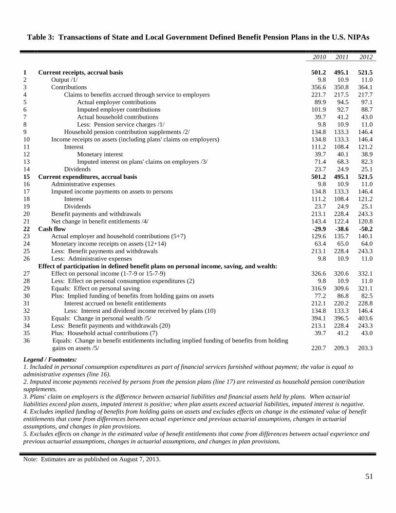
51

Table 3: Transactions of State and Local Government Defined Benefit Pension Plans in the U.S. NIPAs

2010 2011 2012

1 Current receipts, accrual basis 501.2 495.1 521.5

2 Output /1/ 9.8 10.9 11.0

3 Contributions 356.6 350.8 364.1

4 Claims to benefits accrued through service to employers 221.7 217.5 217.7

5 Actual employer contributions 89.9 94.5 97.1

6 Imputed employer contributions 101.9 92.7 88.7

7 Actual household contributions 39.7 41.2 43.0

8 Less: Pension service charges /1/ 9.8 10.9 11.0

9 Household pension contribution supplements /2/ 134.8 133.3 146.4

10 Income receipts on assets (including plans' claims on employers) 134.8 133.3 146.4

11 Interest 111.2 108.4 121.2

12 Monetary interest 39.7 40.1 38.9

13 Imputed interest on plans' claims on employers /3/ 71.4 68.3 82.3

14 Dividends 23.7 24.9 25.1

15 Current expenditures, accrual basis 501.2 495.1 521.5

16 Administrative expenses 9.8 10.9 11.0

17 Imputed income payments on assets to persons 134.8 133.3 146.4

18 Interest 111.2 108.4 121.2

19 Dividends 23.7 24.9 25.1

20 Benefit payments and withdrawals 213.1 228.4 243.3

21 Net change in benefit entitlements /4/ 143.4 122.4 120.8

22 Cash flow -29.9 -38.6 -50.2

23 Actual employer and household contributions (5+7) 129.6 135.7 140.1

24 Monetary income receipts on assets (12+14) 63.4 65.0 64.0

25 Less: Benefit payments and withdrawals 213.1 228.4 243.3

26 Less: Administrative expenses 9.8 10.9 11.0

Effect of participation in defined benefit plans on personal income, saving, and wealth: 27 Effect on personal income (1-7-9 or 15-7-9) 326.6 320.6 332.1

28 Less: Effect on personal consumption expenditures (2) 9.8 10.9 11.0

29 Equals: Effect on personal saving 316.9 309.6 321.1

30 Plus: Implied funding of benefits from holding gains on assets 77.2 86.8 82.5

31 Interest accrued on benefit entitlements 212.1 220.2 228.8

32 Less: Interest and dividend income received by plans (10) 134.8 133.3 146.4

33 Equals: Change in personal wealth /5/ 394.1 396.5 403.6

34 Less: Benefit payments and withdrawals (20) 213.1 228.4 243.3

35 Plus: Household actual contributions (7) 39.7 41.2 43.0

36 Equals: Change in benefit entitlements including implied funding of benefits from holding

gains on assets /5/ 220.7 209.3 203.3

Legend / Footnotes:

1. Included in personal consumption expenditures as part of financial services furnished without payment; the value is equal to

administrative expenses (line 16).

2. Imputed income payments received by persons from the pension plans (line 17) are reinvested as household pension contribution

supplements.

3. Plans' claim on employers is the difference between actuarial liabilities and financial assets held by plans. When actuarial

liabilities exceed plan assets, imputed interest is positive; when plan assets exceed actuarial liabilities, imputed interest is negative.

4. Excludes implied funding of benefits from holding gains on assets and excludes effects on change in the estimated value of benefit

entitlements that come from differences between actual experience and previous actuarial assumptions, changes in actuarial

assumptions, and changes in plan provisions.

5. Excludes effects on change in the estimated value of benefit entitlements that come from differences between actual experience and

previous actuarial assumptions, changes in actuarial assumptions, and changes in plan provisions.

Note: Estimates are as published on August 7, 2013.

52

Table 4: Transactions of Federal Government Defined Benefit Pension Plans in the U.S. NIPAs

2010 2011 2012

1 Current receipts, accrual basis 357.6 367.9 377.7

2 Output /1/ 0.1 0.1 0.1

3 Contributions 209.5 215.2 220.4

4 Claims to benefits accrued through service to employers 61.5 62.7 63.2

5 Actual employer contributions 144.7 149.2 156.1

6 Imputed employer contributions -87.1 -90.4 -96.5

7 Actual household contributions 4.1 4.0 3.7

8 Less: Pension service charges /1/ 0.1 0.1 0.1

9 Household pension contribution supplements /2/ 148.0 152.5 157.2

10 Income receipts on assets (including plans' claims on employers) 148.0 152.5 157.2

11 Interest 148.0 152.5 157.2

12 Monetary interest 48.7 54.9 54.4

13 Imputed interest on plans' claims on employers /3/ 99.3 97.7 102.8

14 Dividends --- --- ---

15 Current expenditures, accrual basis 357.6 367.9 377.7

16 Administrative expenses 0.1 0.1 0.1

17 Imputed income payments on assets to persons 148.0 152.5 157.2

18 Interest 148.0 152.5 157.2

19 Dividends --- --- ---

20 Benefit payments and withdrawals 123.6 125.2 131.7

21 Net change in benefit entitlements /4/ 85.9 90.0 88.6

22 Cash flow 73.7 82.7 82.3

23 Actual employer and household contributions (5+7) 148.8 153.2 159.8

24 Monetary income receipts on assets (12+14) 48.7 54.9 54.4

25 Less: Benefit payments and withdrawals 123.6 125.2 131.7

26 Less: Administrative expenses 0.1 0.1 0.1

Effect of participation in defined benefit plans on personal income, saving, and wealth:

27 Effect on personal income (1-7-9 or 15-7-9) 205.5 211.4 216.8

28 Less: Effect on personal consumption expenditures (2) 0.1 0.1 0.1

29 Equals: Effect on personal saving 205.4 211.2 216.6

30 Plus: Implied funding of benefits from holding gains on assets 0.0 0.0 0.0

31 Interest accrued on benefit entitlements 148.0 152.5 157.2

32 Less: Interest and dividend income received by plans (10) 148.0 152.5 157.2

33 Equals: Change in personal wealth /5/ 205.4 211.2 216.6

34 Less: Benefit payments and withdrawals (20) 123.6 125.2 131.7

35 Plus: Household actual contributions (7) 4.1 4.0 3.7

36 Equals: Change in benefit entitlements including implied funding of benefits from holding

gains on assets /5/ 85.9 90.0 88.6

Legend / Footnotes:

1. Included in personal consumption expenditures as part of financial services furnished without payment; the value is equal to

administrative expenses (line 16).

2. Imputed income payments received by persons from the pension plans (line 17) are reinvested as household pension contribution

supplements.

3. Plans' claim on employers is the difference between actuarial liabilities and financial assets held by plans. When actuarial

liabilities exceed plan assets, imputed interest is positive; when plan assets exceed actuarial liabilities, imputed interest is negative.

4. Excludes implied funding of benefits from holding gains on assets and excludes effects on change in the estimated value of benefit

entitlements that come from differences between actual experience and previous actuarial assumptions, changes in actuarial

assumptions, and changes in plan provisions.

5. Excludes effects on change in the estimated value of benefit entitlements that come from differences between actual experience and

previous actuarial assumptions, changes in actuarial assumptions, and changes in plan provisions.

Note: Estimates are as published on August 7, 2013.

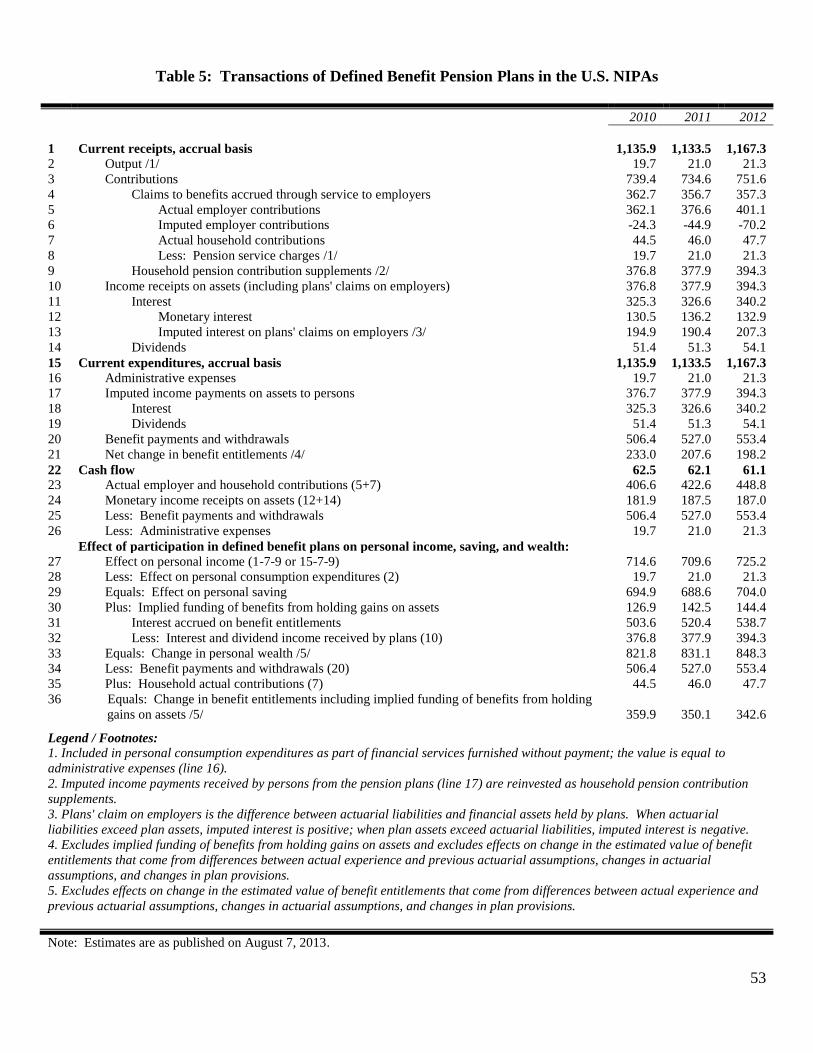
53

Table 5: Transactions of Defined Benefit Pension Plans in the U.S. NIPAs

2010 2011 2012

1 Current receipts, accrual basis 1,135.9 1,133.5 1,167.3

2 Output /1/ 19.7 21.0 21.3

3 Contributions 739.4 734.6 751.6

4 Claims to benefits accrued through service to employers 362.7 356.7 357.3

5 Actual employer contributions 362.1 376.6 401.1

6 Imputed employer contributions -24.3 -44.9 -70.2

7 Actual household contributions 44.5 46.0 47.7

8 Less: Pension service charges /1/ 19.7 21.0 21.3

9 Household pension contribution supplements /2/ 376.8 377.9 394.3

10 Income receipts on assets (including plans' claims on employers) 376.8 377.9 394.3

11 Interest 325.3 326.6 340.2

12 Monetary interest 130.5 136.2 132.9

13 Imputed interest on plans' claims on employers /3/ 194.9 190.4 207.3

14 Dividends 51.4 51.3 54.1

15 Current expenditures, accrual basis 1,135.9 1,133.5 1,167.3

16 Administrative expenses 19.7 21.0 21.3

17 Imputed income payments on assets to persons 376.7 377.9 394.3

18 Interest 325.3 326.6 340.2

19 Dividends 51.4 51.3 54.1

20 Benefit payments and withdrawals 506.4 527.0 553.4

21 Net change in benefit entitlements /4/ 233.0 207.6 198.2

22 Cash flow 62.5 62.1 61.1

23 Actual employer and household contributions (5+7) 406.6 422.6 448.8

24 Monetary income receipts on assets (12+14) 181.9 187.5 187.0

25 Less: Benefit payments and withdrawals 506.4 527.0 553.4

26 Less: Administrative expenses 19.7 21.0 21.3

Effect of participation in defined benefit plans on personal income, saving, and wealth:

27 Effect on personal income (1-7-9 or 15-7-9) 714.6 709.6 725.2

28 Less: Effect on personal consumption expenditures (2) 19.7 21.0 21.3

29 Equals: Effect on personal saving 694.9 688.6 704.0

30 Plus: Implied funding of benefits from holding gains on assets 126.9 142.5 144.4

31 Interest accrued on benefit entitlements 503.6 520.4 538.7

32 Less: Interest and dividend income received by plans (10) 376.8 377.9 394.3

33 Equals: Change in personal wealth /5/ 821.8 831.1 848.3

34 Less: Benefit payments and withdrawals (20) 506.4 527.0 553.4

35 Plus: Household actual contributions (7) 44.5 46.0 47.7

36 Equals: Change in benefit entitlements including implied funding of benefits from holding

gains on assets /5/ 359.9 350.1 342.6

Legend / Footnotes:

1. Included in personal consumption expenditures as part of financial services furnished without payment; the value is equal to

administrative expenses (line 16).

2. Imputed income payments received by persons from the pension plans (line 17) are reinvested as household pension contribution

supplements.

3. Plans' claim on employers is the difference between actuarial liabilities and financial assets held by plans. When actuarial

liabilities exceed plan assets, imputed interest is positive; when plan assets exceed actuarial liabilities, imputed interest is negative.

4. Excludes implied funding of benefits from holding gains on assets and excludes effects on change in the estimated value of benefit

entitlements that come from differences between actual experience and previous actuarial assumptions, changes in actuarial

assumptions, and changes in plan provisions.

5. Excludes effects on change in the estimated value of benefit entitlements that come from differences between actual experience and

previous actuarial assumptions, changes in actuarial assumptions, and changes in plan provisions.

Note: Estimates are as published on August 7, 2013.

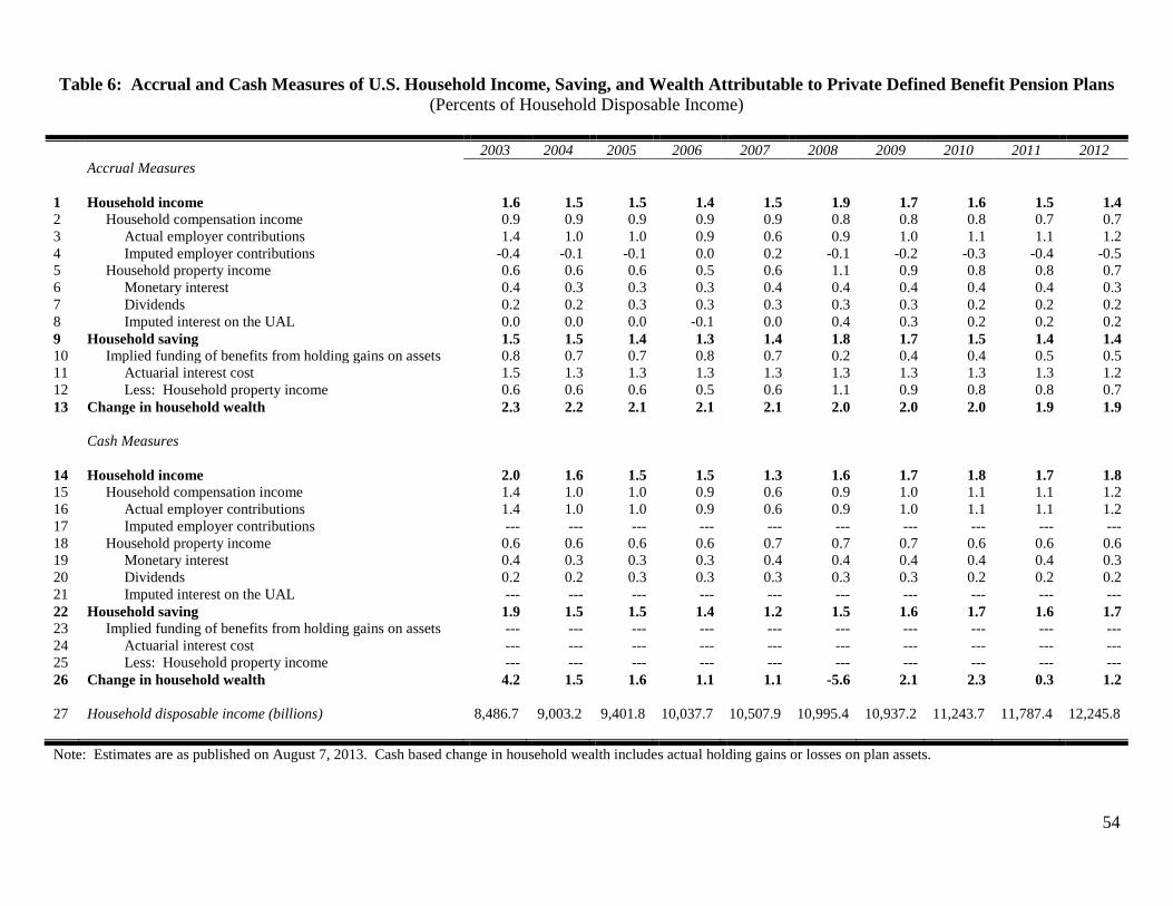
54

Table 6: Accrual and Cash Measures of U.S. Household Income, Saving, and Wealth Attributable to Private Defined Benefit Pension Plans

(Percents of Household Disposable Income)

2003 2004 2005 2006 2007 2008 2009 2010 2011 2012

Accrual Measures

1 Household income 1.6 1.5 1.5 1.4 1.5 1.9 1.7 1.6 1.5 1.4

2 Household compensation income 0.9 0.9 0.9 0.9 0.9 0.8 0.8 0.8 0.7 0.7

3 Actual employer contributions 1.4 1.0 1.0 0.9 0.6 0.9 1.0 1.1 1.1 1.2

4 Imputed employer contributions -0.4 -0.1 -0.1 0.0 0.2 -0.1 -0.2 -0.3 -0.4 -0.5

5 Household property income 0.6 0.6 0.6 0.5 0.6 1.1 0.9 0.8 0.8 0.7

6 Monetary interest 0.4 0.3 0.3 0.3 0.4 0.4 0.4 0.4 0.4 0.3

7 Dividends 0.2 0.2 0.3 0.3 0.3 0.3 0.3 0.2 0.2 0.2

8 Imputed interest on the UAL 0.0 0.0 0.0 -0.1 0.0 0.4 0.3 0.2 0.2 0.2

9 Household saving 1.5 1.5 1.4 1.3 1.4 1.8 1.7 1.5 1.4 1.4

10 Implied funding of benefits from holding gains on assets 0.8 0.7 0.7 0.8 0.7 0.2 0.4 0.4 0.5 0.5

11 Actuarial interest cost 1.5 1.3 1.3 1.3 1.3 1.3 1.3 1.3 1.3 1.2

12 Less: Household property income 0.6 0.6 0.6 0.5 0.6 1.1 0.9 0.8 0.8 0.7

13 Change in household wealth 2.3 2.2 2.1 2.1 2.1 2.0 2.0 2.0 1.9 1.9

Cash Measures

14 Household income 2.0 1.6 1.5 1.5 1.3 1.6 1.7 1.8 1.7 1.8

15 Household compensation income 1.4 1.0 1.0 0.9 0.6 0.9 1.0 1.1 1.1 1.2

16 Actual employer contributions 1.4 1.0 1.0 0.9 0.6 0.9 1.0 1.1 1.1 1.2

17 Imputed employer contributions --- --- --- --- --- --- --- --- --- ---

18 Household property income 0.6 0.6 0.6 0.6 0.7 0.7 0.7 0.6 0.6 0.6

19 Monetary interest 0.4 0.3 0.3 0.3 0.4 0.4 0.4 0.4 0.4 0.3

20 Dividends 0.2 0.2 0.3 0.3 0.3 0.3 0.3 0.2 0.2 0.2

21 Imputed interest on the UAL --- --- --- --- --- --- --- --- --- ---

22 Household saving 1.9 1.5 1.5 1.4 1.2 1.5 1.6 1.7 1.6 1.7

23 Implied funding of benefits from holding gains on assets --- --- --- --- --- --- --- --- --- ---

24 Actuarial interest cost --- --- --- --- --- --- --- --- --- ---

25 Less: Household property income --- --- --- --- --- --- --- --- --- ---

26 Change in household wealth 4.2 1.5 1.6 1.1 1.1 -5.6 2.1 2.3 0.3 1.2

27 Household disposable income (billions) 8,486.7 9,003.2 9,401.8 10,037.7 10,507.9 10,995.4 10,937.2 11,243.7 11,787.4 12,245.8

Note: Estimates are as published on August 7, 2013. Cash based change in household wealth includes actual holding gains or losses on plan assets.

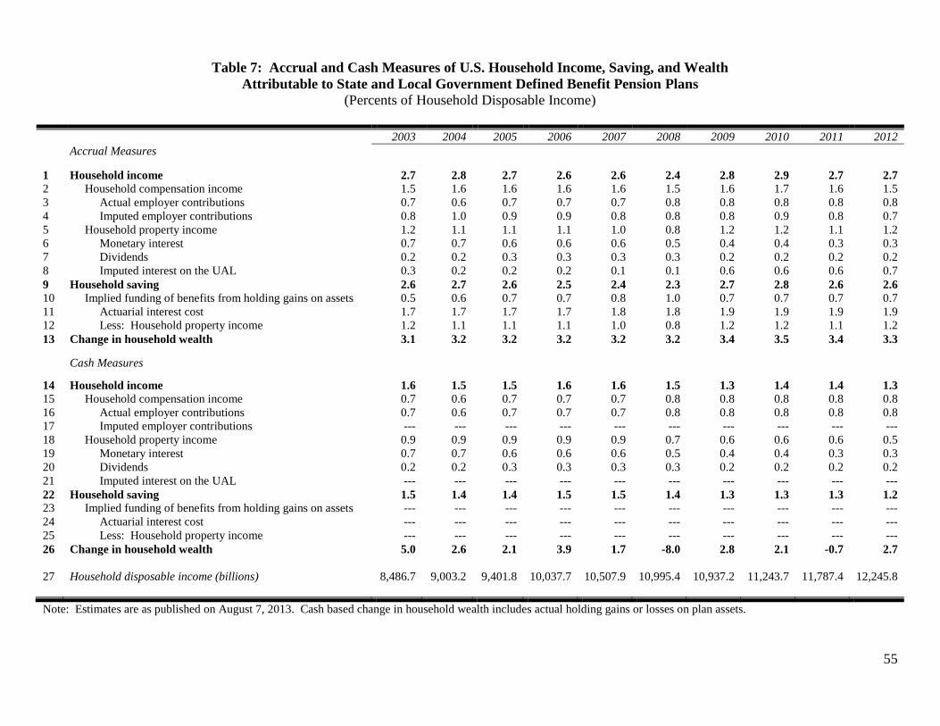
55

Table 7: Accrual and Cash Measures of U.S. Household Income, Saving, and Wealth

Attributable to State and Local Government Defined Benefit Pension Plans

(Percents of Household Disposable Income)

2003 2004 2005 2006 2007 2008 2009 2010 2011 2012

Accrual Measures

1 Household income 2.7 2.8 2.7 2.6 2.6 2.4 2.8 2.9 2.7 2.7

2 Household compensation income 1.5 1.6 1.6 1.6 1.6 1.5 1.6 1.7 1.6 1.5

3 Actual employer contributions 0.7 0.6 0.7 0.7 0.7 0.8 0.8 0.8 0.8 0.8

4 Imputed employer contributions 0.8 1.0 0.9 0.9 0.8 0.8 0.8 0.9 0.8 0.7

5 Household property income 1.2 1.1 1.1 1.1 1.0 0.8 1.2 1.2 1.1 1.2

6 Monetary interest 0.7 0.7 0.6 0.6 0.6 0.5 0.4 0.4 0.3 0.3

7 Dividends 0.2 0.2 0.3 0.3 0.3 0.3 0.2 0.2 0.2 0.2

8 Imputed interest on the UAL 0.3 0.2 0.2 0.2 0.1 0.1 0.6 0.6 0.6 0.7

9 Household saving 2.6 2.7 2.6 2.5 2.4 2.3 2.7 2.8 2.6 2.6

10 Implied funding of benefits from holding gains on assets 0.5 0.6 0.7 0.7 0.8 1.0 0.7 0.7 0.7 0.7

11 Actuarial interest cost 1.7 1.7 1.7 1.7 1.8 1.8 1.9 1.9 1.9 1.9

12 Less: Household property income 1.2 1.1 1.1 1.1 1.0 0.8 1.2 1.2 1.1 1.2

13 Change in household wealth 3.1 3.2 3.2 3.2 3.2 3.2 3.4 3.5 3.4 3.3

Cash Measures

14 Household income 1.6 1.5 1.5 1.6 1.6 1.5 1.3 1.4 1.4 1.3

15 Household compensation income 0.7 0.6 0.7 0.7 0.7 0.8 0.8 0.8 0.8 0.8

16 Actual employer contributions 0.7 0.6 0.7 0.7 0.7 0.8 0.8 0.8 0.8 0.8

17 Imputed employer contributions --- --- --- --- --- --- --- --- --- ---

18 Household property income 0.9 0.9 0.9 0.9 0.9 0.7 0.6 0.6 0.6 0.5

19 Monetary interest 0.7 0.7 0.6 0.6 0.6 0.5 0.4 0.4 0.3 0.3

20 Dividends 0.2 0.2 0.3 0.3 0.3 0.3 0.2 0.2 0.2 0.2

21 Imputed interest on the UAL --- --- --- --- --- --- --- --- --- ---

22 Household saving 1.5 1.4 1.4 1.5 1.5 1.4 1.3 1.3 1.3 1.2

23 Implied funding of benefits from holding gains on assets --- --- --- --- --- --- --- --- --- ---

24 Actuarial interest cost --- --- --- --- --- --- --- --- --- ---

25 Less: Household property income --- --- --- --- --- --- --- --- --- ---

26 Change in household wealth 5.0 2.6 2.1 3.9 1.7 -8.0 2.8 2.1 -0.7 2.7

27 Household disposable income (billions) 8,486.7 9,003.2 9,401.8 10,037.7 10,507.9 10,995.4 10,937.2 11,243.7 11,787.4 12,245.8

Note: Estimates are as published on August 7, 2013. Cash based change in household wealth includes actual holding gains or losses on plan assets.

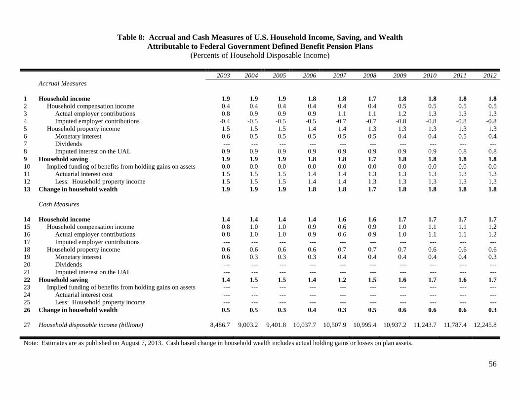
56

Table 8: Accrual and Cash Measures of U.S. Household Income, Saving, and Wealth

Attributable to Federal Government Defined Benefit Pension Plans

(Percents of Household Disposable Income)

2003 2004 2005 2006 2007 2008 2009 2010 2011 2012

Accrual Measures

1 Household income 1.9 1.9 1.9 1.8 1.8 1.7 1.8 1.8 1.8 1.8

2 Household compensation income 0.4 0.4 0.4 0.4 0.4 0.4 0.5 0.5 0.5 0.5

3 Actual employer contributions 0.8 0.9 0.9 0.9 1.1 1.1 1.2 1.3 1.3 1.3

4 Imputed employer contributions -0.4 -0.5 -0.5 -0.5 -0.7 -0.7 -0.8 -0.8 -0.8 -0.8

5 Household property income 1.5 1.5 1.5 1.4 1.4 1.3 1.3 1.3 1.3 1.3

6 Monetary interest 0.6 0.5 0.5 0.5 0.5 0.5 0.4 0.4 0.5 0.4

7 Dividends --- --- --- --- --- --- --- --- --- ---

8 Imputed interest on the UAL 0.9 0.9 0.9 0.9 0.9 0.9 0.9 0.9 0.8 0.8

9 Household saving 1.9 1.9 1.9 1.8 1.8 1.7 1.8 1.8 1.8 1.8

10 Implied funding of benefits from holding gains on assets 0.0 0.0 0.0 0.0 0.0 0.0 0.0 0.0 0.0 0.0

11 Actuarial interest cost 1.5 1.5 1.5 1.4 1.4 1.3 1.3 1.3 1.3 1.3

12 Less: Household property income 1.5 1.5 1.5 1.4 1.4 1.3 1.3 1.3 1.3 1.3

13 Change in household wealth 1.9 1.9 1.9 1.8 1.8 1.7 1.8 1.8 1.8 1.8

Cash Measures

14 Household income 1.4 1.4 1.4 1.4 1.6 1.6 1.7 1.7 1.7 1.7

15 Household compensation income 0.8 1.0 1.0 0.9 0.6 0.9 1.0 1.1 1.1 1.2

16 Actual employer contributions 0.8 1.0 1.0 0.9 0.6 0.9 1.0 1.1 1.1 1.2

17 Imputed employer contributions --- --- --- --- --- --- --- --- --- ---

18 Household property income 0.6 0.6 0.6 0.6 0.7 0.7 0.7 0.6 0.6 0.6

19 Monetary interest 0.6 0.3 0.3 0.3 0.4 0.4 0.4 0.4 0.4 0.3

20 Dividends --- --- --- --- --- --- --- --- --- ---

21 Imputed interest on the UAL --- --- --- --- --- --- --- --- --- ---

22 Household saving 1.4 1.5 1.5 1.4 1.2 1.5 1.6 1.7 1.6 1.7

23 Implied funding of benefits from holding gains on assets --- --- --- --- --- --- --- --- --- ---

24 Actuarial interest cost --- --- --- --- --- --- --- --- --- ---

25 Less: Household property income --- --- --- --- --- --- --- --- --- ---

26 Change in household wealth 0.5 0.5 0.3 0.4 0.3 0.5 0.6 0.6 0.6 0.3

27 Household disposable income (billions) 8,486.7 9,003.2 9,401.8 10,037.7 10,507.9 10,995.4 10,937.2 11,243.7 11,787.4 12,245.8

Note: Estimates are as published on August 7, 2013. Cash based change in household wealth includes actual holding gains or losses on plan assets.

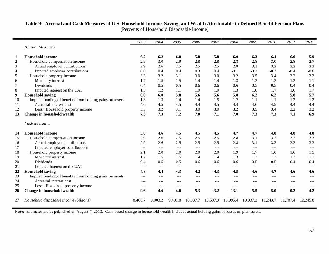
57

Table 9: Accrual and Cash Measures of U.S. Household Income, Saving, and Wealth Attributable to Defined Benefit Pension Plans

(Percents of Household Disposable Income)

2003 2004 2005 2006 2007 2008 2009 2010 2011 2012

Accrual Measures

1 Household income 6.2 6.2 6.0 5.8 5.8 6.0 6.3 6.4 6.0 5.9

2 Household compensation income 2.9 3.0 2.9 2.8 2.8 2.8 2.8 3.0 2.8 2.7

3 Actual employer contributions 2.9 2.6 2.5 2.5 2.5 2.8 3.1 3.2 3.2 3.3

4 Imputed employer contributions 0.0 0.4 0.4 0.3 0.4 -0.1 -0.2 -0.2 -0.4 -0.6

5 Household property income 3.3 3.2 3.1 3.0 3.0 3.2 3.5 3.4 3.2 3.2

6 Monetary interest 1.7 1.5 1.5 1.4 1.4 1.3 1.2 1.2 1.2 1.1

7 Dividends 0.4 0.5 0.5 0.6 0.6 0.6 0.5 0.5 0.4 0.4

8 Imputed interest on the UAL 1.3 1.2 1.1 1.0 1.0 1.3 1.8 1.7 1.6 1.7

9 Household saving 6.0 6.0 5.8 5.6 5.6 5.8 6.2 6.2 5.8 5.7

10 Implied funding of benefits from holding gains on assets 1.3 1.3 1.4 1.4 1.5 1.2 1.1 1.1 1.2 1.2

11 Actuarial interest cost 4.6 4.5 4.5 4.4 4.5 4.4 4.6 4.5 4.4 4.4

12 Less: Household property income 3.3 3.2 3.1 3.0 3.0 3.2 3.5 3.4 3.2 3.2

13 Change in household wealth 7.3 7.3 7.2 7.0 7.1 7.0 7.3 7.3 7.1 6.9

Cash Measures

14 Household income 5.0 4.6 4.5 4.5 4.5 4.7 4.7 4.8 4.8 4.8

15 Household compensation income 2.9 2.6 2.5 2.5 2.5 2.8 3.1 3.2 3.2 3.3

16 Actual employer contributions 2.9 2.6 2.5 2.5 2.5 2.8 3.1 3.2 3.2 3.3

17 Imputed employer contributions --- --- --- --- --- --- --- --- --- ---

18 Household property income 2.1 2.0 2.0 2.0 2.0 1.9 1.7 1.6 1.6 1.5

19 Monetary interest 1.7 1.5 1.5 1.4 1.4 1.3 1.2 1.2 1.2 1.1

20 Dividends 0.4 0.5 0.5 0.6 0.6 0.6 0.5 0.5 0.4 0.4

21 Imputed interest on the UAL --- --- --- --- --- --- --- --- --- ---

22 Household saving 4.8 4.4 4.3 4.2 4.3 4.5 4.6 4.7 4.6 4.6

23 Implied funding of benefits from holding gains on assets --- --- --- --- --- --- --- --- --- ---

24 Actuarial interest cost --- --- --- --- --- --- --- --- --- ---

25 Less: Household property income --- --- --- --- --- --- --- --- --- ---

26 Change in household wealth 9.6 4.6 4.0 5.3 3.2 -13.1 5.5 5.0 0.2 4.2

27 Household disposable income (billions) 8,486.7 9,003.2 9,401.8 10,037.7 10,507.9 10,995.4 10,937.2 11,243.7 11,787.4 12,245.8

Note: Estimates are as published on August 7, 2013. Cash based change in household wealth includes actual holding gains or losses on plan assets.

58

Appendix A. Adjusting Actuarial Estimates to a Common Discount Rate

There are three methods to adjust actuarial estimates to reflect a single discount rate across

multiple pension plans: termination formula, alternative calculation method (ACM) formula, and

uniform distribution formula. Each formula yields a factor by which the actuarial estimate can be

multiplied. Let r denote the discount rate assumed in the actuarial estimate, and let r* denote the

desired single discount rate.

The termination formulas to calculate adjustment factors for retired and non-retired participants

are provided by PBGC as follows:

(A.1) )*()*(38.5Re 00460782.0 rrrrtired eTerm

and

(A.2) )*()*(02.15 0000003.0 rrrrretiredNon eTerm .

The ACM formulas to calculate adjustment factors for retired and non-retired participants are

provided by PBGC as follows, where Age is the average retirement age:

(A.3) )*()*(100Re 00205487.094.0 rrrrtiredACM

and

(A.4) 50)*(100 *)]1/()1[(94.0 AgerrretiredNon rrACM .

If r* > r, equations (A.1) through (A.4) yield factors less than 1. In this case, actuarial

estimates will be adjusted downward to reflect the higher than assumed discount rate.

Termination formulas are used by PBGC to adjust termination liabilities for plans taken over by

PBGC. The ACM formulas are used by PBGC for general purposes. Given the obscurity of the

underlying assumptions for each set of formulas used by PBGC, we use an alternative set of formulas

to adjust actuarial estimates. The alternative set of formulas assumes a uniform distribution of years of

retirement, denoted NYR. The alternative set also assumes a uniform distribution of years until

retirement, denoted NYA, with each cohort receiving an annuity that is paid out over a number of years

59

upon retirement. The formulas to calculate adjustment factors for retired and non-retired participants

under the uniform distribution are as follows:

(A.5)

))1(1()(

)*)1(1(*)(

1

*1

*

2

Re

NYR

NYRtired

rrNYR

rrNYR

r

r

r

rUniform

and

(A.6)

NYA

NYA

NYR

NYRretiredNon

r

r

r

r

r

r

r

rUniform

)1(1

*)1(1

)1(1

*)1(1

1

*1

*

2

.

One use of equation (A.5) is to adjust actuarial estimates of benefits payable to retired

participants. One use of equation (A.6) is to adjust actuarial estimates of normal cost for non-retired

participants. To adjust actuarial estimates of the actuarial liability, which includes amounts for retired

and non-retired participants, equations (A.5) and (A.6) can be combined with weights to distinguish

retired participants from non-retired participants. The following equation in which denotes the

weight for retired participants, shows the adjustment factor for current liability under the uniform

distribution:

(A.7)

r

r

r

rUniformLiability

1

*1

*

2

NYA

NYA

NYR

NYR

NYR

NYR

r

r

r

r

rrNYR

rrNYR

)1(1

*)1(1

)1(1

*)1(1)1(

))1(1()(

)*)1(1(*)( .

We determine the weight in equation (A.7) by dividing the aggregate actuarial liability for retired

participants by the aggregate actuarial liability for active and retired participants. We use the formulas

in equations (A.5) through (A.7) to adjust the normal cost and the actuarial liability across plans to a

common discount rate. Additional information on adjusting actuarial estimates to a common discount

rate can be found in Applebaum (1992) and Ippolito (1986).

60

Appendix B. Discount Rate Assumptions for the U.S. NIPAs

We use the same discount rate series for private plans and state and local plans. For federal

plans, we use different discount rate series for civilian plans and military plans. The discount rate

series for private plans and state and local plans are presented in table B1, and the series for federal

plans are presented in table B2.

Private Plans and State and Local Plans

For private plans and state and local plans, we assume a discount rate series using the AAA

corporate bond yields published by the FRB, table H.15, as a reference series. We apply four decision

criteria. First, in addition to using corporate bond yields as a reference series, we use 5 – 7 percent as a

target range for all long-term trends because the averages of all our references hover around 6 percent

over time. For example, the average AAA corporate bond yield from 1929 to 2008 is 6.0 percent, the

average discount rate used by PBGC from 1979 to 2008 is 6.8 percent, and the median discount rate

reported by plans on form 5500 is approximately 6.0 percent from 2000 to 2009. Second, we do not let

the rate change more than once in a consecutive three-year period. Third, the top rate in our series is

9.5 percent based on PBGC’s published rates for the early 1980s. In the early 1980s, corporate bond

yields were as high as 14 percent in 1981. PBGC’s rate is 11 percent in 1986 but under 10 percent in

all surrounding years. We know now the high rates in the 1980s were not sustainable. Fourth, we

generally do not let the discount rate change more than one percentage point from one year to the next

except immediately preceding the early 1980s when corporate bond rates were at their highest. We

allow the rate to increase two percentage points from 1979 to 1980 in order to meet the second

criterion. A one percentage point increase (decrease) in the discount rate generally decreases

(increases) the normal cost by approximately 12 percentage points. Table B1 presents the series for

private plans and state and local plans.

For state and local plans, GASB sanctions the use of the expected investment rate of return for

61

discounting purposes in defiance of finance theory which states that the appropriate discount rate

reflects the risk of the liability. Until recently, economists often argued that state and local government

pension liabilities were riskless and that a rate such as the rate for U.S. Treasury securities (adjusted

for things such as their exemption from state and local taxes, their liquidity, and their status as safe

havens in times of financial stress) should be used. Advocates of a riskless rate of return cited

historical experience—no state or local government had ever reduced benefits, even on occasions when

losses were incurred by bondholders. Advocates also cited the legal and constitutional protections on

state and local government pensions (Brown and Wilcox 2009).

More recently, states have reduced their pension liabilities by reducing the pension benefits of

current retirees, generally by reducing or eliminating promised automatic COLAs and by requiring

higher employee contributions. As a consequence, recent experience suggests using a discount rate

higher than that used for federal pensions, whose risk remains unaffected by recent events but lower

than that used for private pensions. In practice, since the rate for federal civilian plans has been greater

than or equal to the rate for private plans since 1989 (tables B1 and B2), we decided to use the private

plan discount rate for state and local government pension plans.26

Federal Plans

For federal plans, we assume the same discount rates used by federal actuaries and published in

the annual reports for civilian plans and military plans. While discount rates used by federal actuaries

tend to be high relative to our discount rates for private plans and state and local plans, the rates are

offset by high inflation rate assumptions because of cost of living adjustments and by high wage

growth assumptions because of PBO actuarial methods. Thus, discount rate assumptions by federal

actuaries tend to produce a higher actuarial liability than the assumptions used for private plans and

26

For comparison of federal plans to private plans, the U.S. Congressional Budget Office also uses the same discount rate

across sectors (Falk, 2012). The rate selected is about 1 percent higher than the rate of return on 20-year nominal treasury

securities in 2009. Moody’s Investors Service (2013) also uses a high-grade long-term corporate bond index as the discount

rate to adjust state and local government reported pension data.

62

state and local plans. Discount rate assumptions for federal civilian plans and federal military plans do

not always agree, so table B2 presents the separate series for civilian plans and military plans.

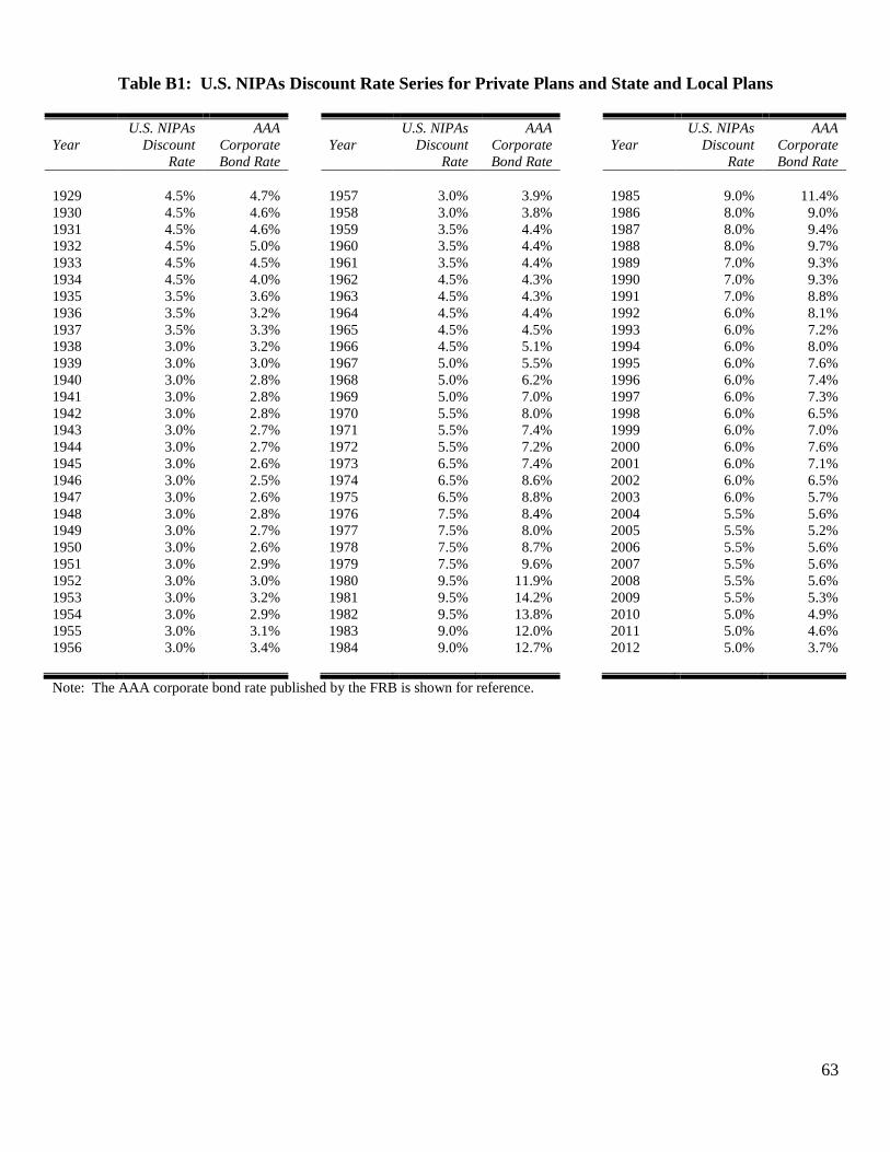
63

Table B1: U.S. NIPAs Discount Rate Series for Private Plans and State and Local Plans

Year

U.S. NIPAs

Discount

Rate

AAA

Corporate

Bond Rate

Year

U.S. NIPAs

Discount

Rate

AAA

Corporate

Bond Rate

Year

U.S. NIPAs

Discount

Rate

AAA

Corporate

Bond Rate

1929 4.5% 4.7% 1957 3.0% 3.9% 1985 9.0% 11.4%

1930 4.5% 4.6% 1958 3.0% 3.8% 1986 8.0% 9.0%

1931 4.5% 4.6% 1959 3.5% 4.4% 1987 8.0% 9.4%

1932 4.5% 5.0% 1960 3.5% 4.4% 1988 8.0% 9.7%

1933 4.5% 4.5% 1961 3.5% 4.4% 1989 7.0% 9.3%

1934 4.5% 4.0% 1962 4.5% 4.3% 1990 7.0% 9.3%

1935 3.5% 3.6% 1963 4.5% 4.3% 1991 7.0% 8.8%

1936 3.5% 3.2% 1964 4.5% 4.4% 1992 6.0% 8.1%

1937 3.5% 3.3% 1965 4.5% 4.5% 1993 6.0% 7.2%

1938 3.0% 3.2% 1966 4.5% 5.1% 1994 6.0% 8.0%

1939 3.0% 3.0% 1967 5.0% 5.5% 1995 6.0% 7.6%

1940 3.0% 2.8% 1968 5.0% 6.2% 1996 6.0% 7.4%

1941 3.0% 2.8% 1969 5.0% 7.0% 1997 6.0% 7.3%

1942 3.0% 2.8% 1970 5.5% 8.0% 1998 6.0% 6.5%

1943 3.0% 2.7% 1971 5.5% 7.4% 1999 6.0% 7.0%

1944 3.0% 2.7% 1972 5.5% 7.2% 2000 6.0% 7.6%

1945 3.0% 2.6% 1973 6.5% 7.4% 2001 6.0% 7.1%

1946 3.0% 2.5% 1974 6.5% 8.6% 2002 6.0% 6.5%

1947 3.0% 2.6% 1975 6.5% 8.8% 2003 6.0% 5.7%

1948 3.0% 2.8% 1976 7.5% 8.4% 2004 5.5% 5.6%

1949 3.0% 2.7% 1977 7.5% 8.0% 2005 5.5% 5.2%

1950 3.0% 2.6% 1978 7.5% 8.7% 2006 5.5% 5.6%

1951 3.0% 2.9% 1979 7.5% 9.6% 2007 5.5% 5.6%

1952 3.0% 3.0% 1980 9.5% 11.9% 2008 5.5% 5.6%

1953 3.0% 3.2% 1981 9.5% 14.2% 2009 5.5% 5.3%

1954 3.0% 2.9% 1982 9.5% 13.8% 2010 5.0% 4.9%

1955 3.0% 3.1% 1983 9.0% 12.0% 2011 5.0% 4.6%

1956 3.0% 3.4% 1984 9.0% 12.7% 2012 5.0% 3.7%

Note: The AAA corporate bond rate published by the FRB is shown for reference.

64

Table B2: U.S. NIPAs Discount Rate Series for Federal Plans

Year Civilian

Plans

Military

Plans Year

Civilian

Plans

Military

Plans

Year

Civilian

Plans

Military

Plans

1929 4.5% 4.5% 1957 4.5% 4.5% 1985 7.0% 7.0%

1930 4.5% 4.5% 1958 4.5% 4.5% 1986 7.0% 7.0%

1931 4.5% 4.5% 1959 4.5% 4.5% 1987 7.0% 7.0%

1932 4.5% 4.5% 1960 4.5% 4.5% 1988 7.0% 7.0%

1933 4.5% 4.5% 1961 4.5% 4.5% 1989 7.0% 7.0%

1934 4.5% 4.5% 1962 4.5% 4.5% 1990 7.0% 7.0%

1935 4.5% 4.5% 1963 4.5% 4.5% 1991 7.0% 7.0%

1936 4.5% 4.5% 1964 4.5% 4.5% 1992 7.0% 7.0%

1937 4.5% 4.5% 1965 4.5% 4.5% 1993 7.0% 7.0%

1938 4.5% 4.5% 1966 4.5% 4.5% 1994 7.0% 6.75%

1939 4.5% 4.5% 1967 4.5% 4.5% 1995 7.0% 6.75%

1940 4.5% 4.5% 1968 4.5% 4.5% 1996 7.0% 6.5%

1941 4.5% 4.5% 1969 4.5% 4.5% 1997 7.0% 6.5%

1942 4.5% 4.5% 1970 4.5% 4.5% 1998 7.0% 6.5%

1943 4.5% 4.5% 1971 6.0% 6.0% 1999 7.0% 6.25%

1944 4.5% 4.5% 1972 6.0% 6.0% 2000 6.75% 6.25% 1945 4.5% 4.5% 1973 6.0% 6.0% 2001 6.75% 6.25% 1946 4.5% 4.5% 1974 6.0% 6.0% 2002 6.25% 6.25% 1947 4.5% 4.5% 1975 6.0% 6.0% 2003 6.25% 6.25% 1948 4.5% 4.5% 1976 6.0% 6.0% 2004 6.25% 6.25% 1949 4.5% 4.5% 1977 6.0% 6.0% 2005 6.25% 6.25% 1950 4.5% 4.5% 1978 7.0% 7.0% 2006 6.25% 6.0%

1951 4.5% 4.5% 1979 7.0% 7.0% 2007 6.25% 6.0%

1952 4.5% 4.5% 1980 7.0% 7.0% 2008 6.25% 5.75%

1953 4.5% 4.5% 1981 7.0% 7.0% 2009 5.75% 5.75%

1954 4.5% 4.5% 1982 7.0% 7.0% 2010 5.25% 5.5%

1955 4.5% 4.5% 1983 7.0% 7.0% 2011 5.25% 5.5%

1956 4.5% 4.5% 1984 7.0% 7.0% 2012 5.25% 5.5%

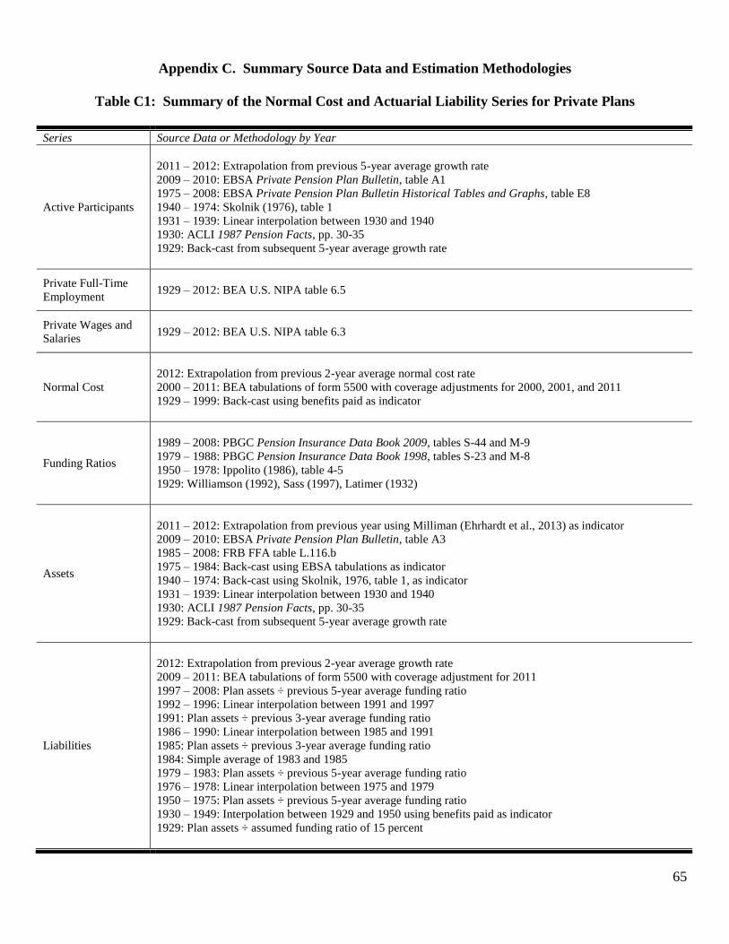
65

Appendix C. Summary Source Data and Estimation Methodologies

Table C1: Summary of the Normal Cost and Actuarial Liability Series for Private Plans

Series Source Data or Methodology by Year

Active Participants

2011 – 2012: Extrapolation from previous 5-year average growth rate

2009 – 2010: EBSA Private Pension Plan Bulletin, table A1

1975 – 2008: EBSA Private Pension Plan Bulletin Historical Tables and Graphs, table E8

1940 – 1974: Skolnik (1976), table 1

1931 – 1939: Linear interpolation between 1930 and 1940

1930: ACLI 1987 Pension Facts, pp. 30-35

1929: Back-cast from subsequent 5-year average growth rate

Private Full-Time

Employment

1929 – 2012: BEA U.S. NIPA table 6.5

Private Wages and

Salaries

1929 – 2012: BEA U.S. NIPA table 6.3

Normal Cost

2012: Extrapolation from previous 2-year average normal cost rate

2000 – 2011: BEA tabulations of form 5500 with coverage adjustments for 2000, 2001, and 2011

1929 – 1999: Back-cast using benefits paid as indicator

Funding Ratios

1989 – 2008: PBGC Pension Insurance Data Book 2009, tables S-44 and M-9

1979 – 1988: PBGC Pension Insurance Data Book 1998, tables S-23 and M-8

1950 – 1978: Ippolito (1986), table 4-5

1929: Williamson (1992), Sass (1997), Latimer (1932)

Assets

2011 – 2012: Extrapolation from previous year using Milliman (Ehrhardt et al., 2013) as indicator

2009 – 2010: EBSA Private Pension Plan Bulletin, table A3

1985 – 2008: FRB FFA table L.116.b

1975 – 1984: Back-cast using EBSA tabulations as indicator

1940 – 1974: Back-cast using Skolnik, 1976, table 1, as indicator

1931 – 1939: Linear interpolation between 1930 and 1940

1930: ACLI 1987 Pension Facts, pp. 30-35

1929: Back-cast from subsequent 5-year average growth rate

Liabilities

2012: Extrapolation from previous 2-year average growth rate

2009 – 2011: BEA tabulations of form 5500 with coverage adjustment for 2011

1997 – 2008: Plan assets ÷ previous 5-year average funding ratio

1992 – 1996: Linear interpolation between 1991 and 1997

1991: Plan assets ÷ previous 3-year average funding ratio

1986 – 1990: Linear interpolation between 1985 and 1991

1985: Plan assets ÷ previous 3-year average funding ratio

1984: Simple average of 1983 and 1985

1979 – 1983: Plan assets ÷ previous 5-year average funding ratio

1976 – 1978: Linear interpolation between 1975 and 1979

1950 – 1975: Plan assets ÷ previous 5-year average funding ratio

1930 – 1949: Interpolation between 1929 and 1950 using benefits paid as indicator

1929: Plan assets ÷ assumed funding ratio of 15 percent

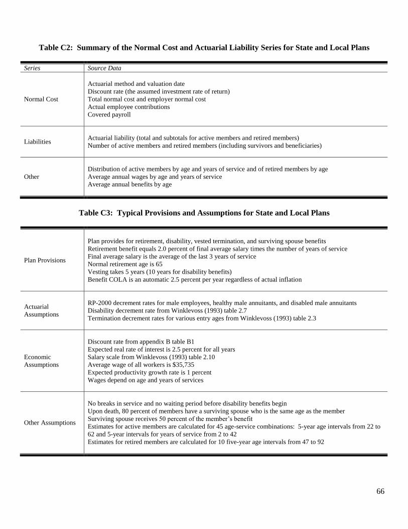
66

Table C2: Summary of the Normal Cost and Actuarial Liability Series for State and Local Plans

Series Source Data

Normal Cost

Actuarial method and valuation date

Discount rate (the assumed investment rate of return)

Total normal cost and employer normal cost

Actual employee contributions

Covered payroll

Liabilities

Actuarial liability (total and subtotals for active members and retired members)

Number of active members and retired members (including survivors and beneficiaries)

Other

Distribution of active members by age and years of service and of retired members by age

Average annual wages by age and years of service

Average annual benefits by age

Table C3: Typical Provisions and Assumptions for State and Local Plans

Plan Provisions

Plan provides for retirement, disability, vested termination, and surviving spouse benefits

Retirement benefit equals 2.0 percent of final average salary times the number of years of service

Final average salary is the average of the last 3 years of service

Normal retirement age is 65

Vesting takes 5 years (10 years for disability benefits)

Benefit COLA is an automatic 2.5 percent per year regardless of actual inflation

Actuarial

Assumptions

RP-2000 decrement rates for male employees, healthy male annuitants, and disabled male annuitants

Disability decrement rate from Winklevoss (1993) table 2.7

Termination decrement rates for various entry ages from Winklevoss (1993) table 2.3

Economic

Assumptions

Discount rate from appendix B table B1

Expected real rate of interest is 2.5 percent for all years

Salary scale from Winklevoss (1993) table 2.10

Average wage of all workers is $35,735

Expected productivity growth rate is 1 percent

Wages depend on age and years of services

Other Assumptions

No breaks in service and no waiting period before disability benefits begin

Upon death, 80 percent of members have a surviving spouse who is the same age as the member

Surviving spouse receives 50 percent of the member’s benefit

Estimates for active members are calculated for 45 age-service combinations: 5-year age intervals from 22 to

62 and 5-year intervals for years of service from 2 to 42

Estimates for retired members are calculated for 10 five-year age intervals from 47 to 92

67

Table C4: Example Normal Cost Estimates for State and Local Plans

A. Entry Age PBO Method

Years of Service

2 7 12 17 22 27 32 37 42

Ag

e

22 581 --- --- --- --- --- --- --- ---

27 1,622 1,141 --- --- --- --- --- --- ---

32 2,221 2,108 1,373 --- --- --- --- --- ---

37 2,578 2,756 2,405 1,540 --- --- --- --- ---

42 2,817 3,126 3,048 2,641 1,620 --- --- --- ---

47 3,124 3,414 3,373 3,285 2,771 1,658 --- --- ---

52 3,382 3,887 3,817 3,792 3,509 2,910 1,842 --- ---

57 3,680 4,206 4,407 4,367 4,157 3,837 3,266 2,035 ---

62 3,370 4,086 4,366 4,737 4,591 4,353 4,005 3,468 2,262

Note: Assumes an 8 percent discount rate.

B. ABO Method

Years of Service

2 7 12 17 22 27 32 37 42

Ag

e

22 232 --- --- --- --- --- --- --- ---

27 641 1,596 --- --- --- --- --- --- ---

32 984 2,355 3,136 --- --- --- --- --- ---

37 1,332 2,979 4,311 5,369 --- --- --- --- ---

42 1,688 3,528 5,192 7,097 8,222 --- --- --- ---

47 2,167 4,185 5,917 8,257 10,687 11,828 --- --- ---

52 2,832 5,265 7,198 9,698 12,518 15,609 17,988 --- ---

57 3,644 6,755 9,132 11,930 15,016 18,956 23,885 26,738 ---

62 4,333 7,685 10,824 14,323 17,867 21,984 27,258 34,498 40,010

Note: Assumes a 5.5 percent discount rate.

C. Distribution of Employment, 2004

Years of Service

2 7 12 17 22 27 32 37 42

Ag

e

22 2.3% --- --- --- --- --- --- --- ---

27 6.5% 1.7% --- --- --- --- --- --- ---

32 5.1% 4.4% 1.2% --- --- --- --- --- ---

37 4.5% 3.7% 3.1% 1.1% --- --- --- --- ---

42 4.0% 3.3% 2.9% 3.0% 1.2% --- --- --- ---

47 3.5% 3.2% 2.8% 2.8% 2.5% 1.1% --- --- ---

52 2.8% 2.7% 2.7% 2.8% 2.2% 2.4% 1.3% --- ---

57 1.8% 1.8% 1.9% 2.1% 1.6% 1.4% 1.6% 0.3% ---

62 1.3% 1.2% 1.2% 1.1% 0.8% 0.7% 0.5% 0.2% 0.1%

68

Table C5: Summary of the Normal Cost and Actuarial Liability Series for Federal Plans

Series Source Data or Methodology by Year

Normal Cost

Civilian Plans

CSRS

1987 – 2012: Actuarial estimates from OPM annual reports plus adjustments for small plans

1929 – 1986: Back-cast using adjusted normal cost rate plus adjustments for small plans when they existed

FERS

1984 – 2012: Actuarial estimates from OPM annual reports plus adjustments for small plans. In recent years

actual contributions are used to estimate the normal cost because the published normal cost rate is the modal

rate, not the average rate, and the actual contributions are extremely close to normal cost.

Military Plans

1985 – 2012: Actuarial estimates from OPM and DOD annual reports plus adjustment for Coast Guard plan

1929 – 1984: Back-cast using adjusted normal cost rate plus adjustment for Coast Guard plan

Liabilities

Civilian Plans

CSRS

1929 – 2012: Simulations that start with initial liability and adjust annually based on equation (4.1)

FERS

1984 – 2012: Simulations that start with zero liability and adjust annually based on equation (4.1)

Military Plans

1929 – 2012: Simulations that start with initial liability and adjust annually based on equation (4.1)