1

Brief Review of the R-Matrix Theory

L. C. Leal

Introduction

Resonance theory deals with the description of the nucleon-nucleus interaction and aims atthe prediction of the experimental structure of cross sections. Resonance theory is basically aninteraction model which treats the nucleus as a black box, whereas nuclear models are concernedwith the description of the nuclear properties based on models of the nuclear forces (nuclearpotential). Any theoretical method of calculating the neutron-nucleus interactions or nuclearproperties cannot fully describe the nuclear effects inside the nucleus because of the complexity ofthe nucleus and because the nuclear forces, acting within the nucleus, are not known in detail.Quantities related to internal properties of the nucleus are taken, in this theory, as parameters whichcan be determined by examining the experimental results.

The general R-matrix theory, introduced by Wigner and Eisenbud in 1947, is a powerfulnuclear interaction model. Despite the generality of the theory, it does not require information aboutthe internal structure of the nucleus; instead, the unknown internal properties, appearing as elementsin the R-matrix, are treated as parameters and can be determined by examining the measured crosssections.

A brief review of the R-matrix theory will be given here and the interaction models whichare specializations of the general R-matrix will be described. The practical aspects of the general R-matrix theory, as well as the relationship between the collision matrix U and the level matrix A withthe R-matrix, will be presented.

Overview of the R-Matrix Theory

The general R-matrix theory has been extensively described by Lane and Thomas. Anoverview is presented here as introduction for the resonance formalisms which will be describedlater.

To understand the basic points of the general R-matrix theory, we will consider a simple caseof neutron collision in which the spin dependence of the constituents of the interactions is neglected.Although the mathematics involved in this special case is over-simplified, it nevertheless containsthe essential elements of the general theory.

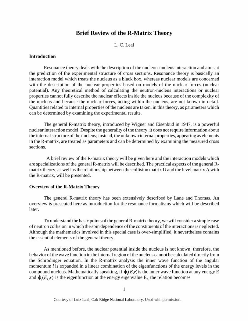
As mentioned before, the nuclear potential inside the nucleus is not known; therefore, thebehavior of the wave function in the internal region of the nucleus cannot be calculated directly fromthe Schrödinger equation. In the R-matrix analysis the inner wave function of the angularmomentum l is expanded in a linear combination of the eigenfunctions of the energy levels in thecompound nucleus. Mathematically speaking, if is the inner wave function at any energy Eand is the eigenfunction at the energy eigenvalue E8, the relation becomes

Courtesy of Luiz Leal, Oak Ridge National Laboratory. Used with permission.

2

(1)

(2)

(3)

(4)

(5)

(6)

Both and are solutions of the radial Schrödinger equations in the internalregion given by

and

Since all terms in this expression must be finite at , both functions vanish at that point.In addition, the logarithmic derivative of the eigenfunction at the nuclear surface, say at , istaken to be constant so that

where is an arbitrary boundary constant.

Since we are dealing with eigenfunctions of a real Hamiltonian, are orthogonal.Assuming that are also normalized, we have

From Eq. (xx-1) and the orthogonality condition, we find the coefficients ,

3

(7)

(8)

(9)

(10)

(11)

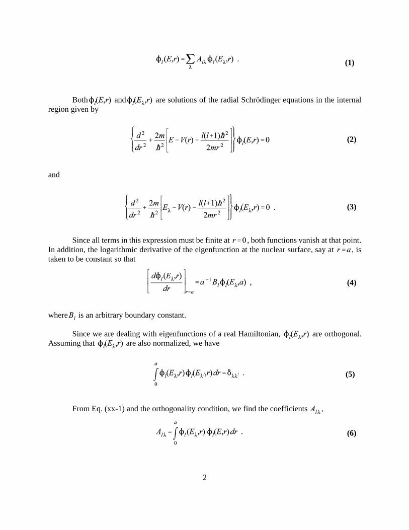
To proceed to the construction of the R-matrix, Eq. (xx-2) is multiplied by and Eq.(xx-3) is multiplied by . Subtracting and integrating the result over the range to (as inEq. (xx-6)) produces the expression for the coefficients :

Inserting into Eq. (xx-1) for r=a at the surface of the nucleus and using Eq. (xx-4), givesthe following expression for the wave function:

Equation (xx-8) relates the value of the inner wave function to its derivative at the surfaceof the nucleus. The R matrix is defined as

or

where , the reduced width amplitude for the level 8 and angular momentum l, is definedas

The reduced width amplitude depends on the value of the inner wave function at the nuclearsurface. Both and are the unknown parameters of the R matrix which can be evaluated byexamining the measured cross sections.

The generalization of Eq. (xx-10) is obtained by including the neutron-nucleus spindependence and several possibilities in which the reaction process can occur. The concept of channelis introduced to designate a possible pair of nucleus and particle and the spin of the pair. Thechannel containing the initial state is called the entrance channel (channel c), whereas, the channel

4

(12)

(13)

(14)

(15)

(16)

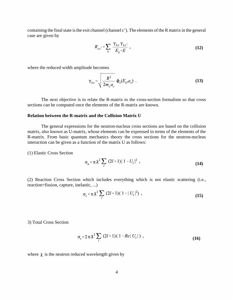
containing the final state is the exit channel (channel c’). The elements of the R matrix in the generalcase are given by

where the reduced width amplitude becomes

The next objective is to relate the R-matrix to the cross-section formalism so that crosssections can be computed once the elements of the R-matrix are known.

Relation between the R-matrix and the Collision Matrix U

The general expressions for the neutron-nucleus cross sections are based on the collisionmatrix, also known as U-matrix, whose elements can be expressed in terms of the elements of theR-matrix. From basic quantum mechanics theory the cross sections for the neutron-nucleusinteraction can be given as a function of the matrix U as follows:

(1) Elastic Cross Section

(2) Reaction Cross Section which includes everything which is not elastic scattering (i.e.,reaction=fission, capture, inelastic, ...)

3) Total Cross Section

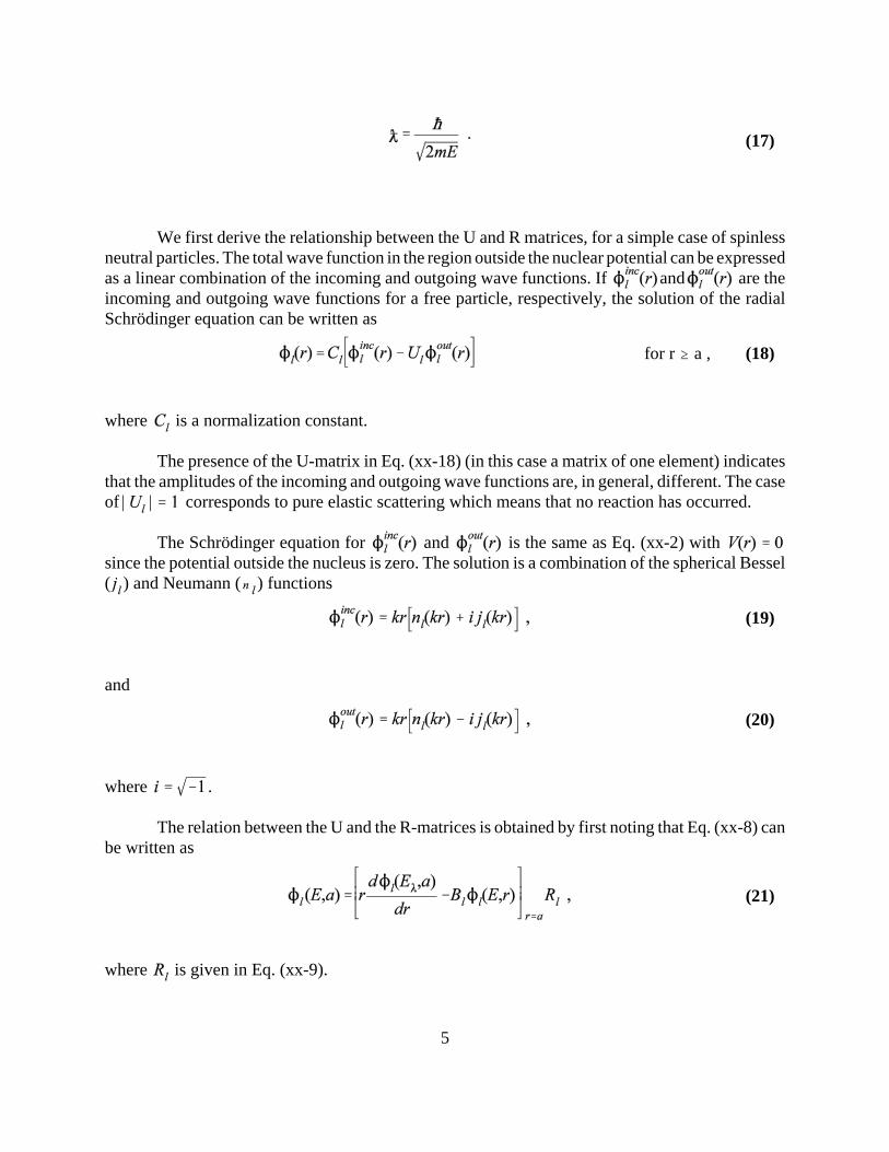
where is the neutron reduced wavelength given by

5

(17)

for r $ a , (18)

(19)

(20)

(21)

We first derive the relationship between the U and R matrices, for a simple case of spinlessneutral particles. The total wave function in the region outside the nuclear potential can be expressedas a linear combination of the incoming and outgoing wave functions. If and are theincoming and outgoing wave functions for a free particle, respectively, the solution of the radialSchrödinger equation can be written as

where is a normalization constant.

The presence of the U-matrix in Eq. (xx-18) (in this case a matrix of one element) indicatesthat the amplitudes of the incoming and outgoing wave functions are, in general, different. The caseof corresponds to pure elastic scattering which means that no reaction has occurred.

The Schrödinger equation for and is the same as Eq. (xx-2) with since the potential outside the nucleus is zero. The solution is a combination of the spherical Bessel( ) and Neumann ( ) functions

and

where .

The relation between the U and the R-matrices is obtained by first noting that Eq. (xx-8) canbe written as

where is given in Eq. (xx-9).

6

(22)

(23)

(24)

(25)

(26)

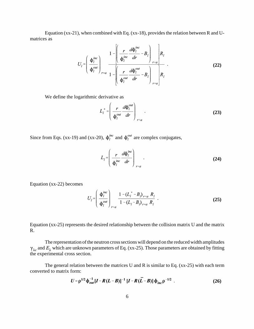
Equation (xx-21), when combined with Eq. (xx-18), provides the relation between R and U-matrices as

We define the logarithmic derivative as

Since from Eqs. (xx-19) and (xx-20), and are complex conjugates,

Equation (xx-22) becomes

Equation (xx-25) represents the desired relationship between the collision matrix U and the matrixR.

The representation of the neutron cross sections will depend on the reduced width amplitudes and which are unknown parameters of Eq. (xx-25). Those parameters are obtained by fitting

the experimental cross section.

The general relation between the matrices U and R is similar to Eq. (xx-25) with each termconverted to matrix form:

7

(27)

(28)

(29)

(30)

All matrices in Eq. (xx-26) are diagonal except the R matrix. The matrix elements of are given by .

It should be noted that no approximation was used in deriving Eq. (xx-26). That equationrepresents an exact expression relating U and R, and leads to the determination of the cross sectionaccording to Eqs. (xx-14, xx-15, and xx-16).

To avoid dealing with matrices of large dimensions, several approximations of the R-matrixtheory have been introduced. We will discuss various of these cross-section formalisms in the pagesto come; we begin by introducing the level matrix A.

Relation between U, R, and A

Another presentation of Eq. (xx-26) may be obtained by introducing the following definitions

and

where S and P are real matrices which contains the shift and the penetration factors, respectivelyand .

From Eqs. (xx-20, xx-23, and xx-27), the penetration factors can be written as, and Eq. (xx-26) becomes

with .

It should be realized that the R-matrix is a channel matrix; i.e. it depends on the entrance andoutgoing channels c and c’. The level matrix concept introduced by Wigner attempts to relate theU matrix to a matrix in which the indices are the energy levels of the compound nucleus, the level

8

(31)

(32)

(33)

(34)

(35)

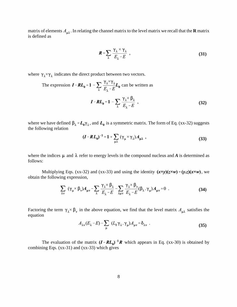
matrix of elements . In relating the channel matrix to the level matrix we recall that the R matrixis defined as

where indicates the direct product between two vectors.

The expression can be written as

where we have defined , and is a symmetric matrix. The form of Eq. (xx-32) suggeststhe following relation

where the indices and refer to energy levels in the compound nucleus and A is determined asfollows:

Multiplying Eqs. (xx-32) and (xx-33) and using the identity , weobtain the following expression,

Factoring the term in the above equation, we find that the level matrix satisfies theequation

The evaluation of the matrix which appears in Eq. (xx-30) is obtained bycombining Eqs. (xx-31) and (xx-33) which gives

9

(36)

(37)

(38)

(39)

(40)

(41)

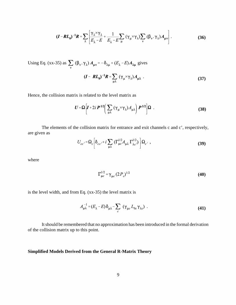
Using Eq. (xx-35) as gives

Hence, the collision matrix is related to the level matrix as

The elements of the collision matrix for entrance and exit channels c and c’, respectively,are given as

where

is the level width, and from Eq. (xx-35) the level matrix is

It should be remembered that no approximation has been introduced in the formal derivationof the collision matrix up to this point.

Simplified Models Derived from the General R-Matrix Theory

10

(42)

(43)

(44)

(45)

(46)

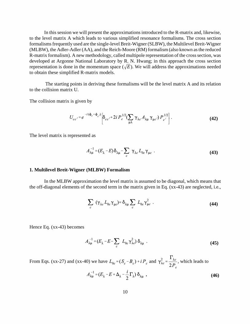
In this session we will present the approximations introduced to the R-matrix and, likewise,to the level matrix A which leads to various simplified resonance formalisms. The cross sectionformalisms frequently used are the single-level Breit-Wigner (SLBW), the Multilevel Breit-Wigner(MLBW), the Adler-Adler (AA), and the Reich-Moore (RM) formalism (also known as the reducedR-matrix formalism). A new methodology, called multipole representation of the cross section, wasdeveloped at Argonne National Laboratory by R. N. Hwang; in this approach the cross sectionrepresentation is done in the momentum space ( ). We will address the approximations neededto obtain these simplified R-matrix models.

The starting points in deriving these formalisms will be the level matrix A and its relationto the collision matrix U.

The collision matrix is given by

The level matrix is represented as

1. Multilevel Breit-Wigner (MLBW) Formalism

In the MLBW approximation the level matrix is assumed to be diagonal, which means thatthe off-diagonal elements of the second term in the matrix given in Eq. (xx-43) are neglected, i.e.,

Hence Eq. (xx-43) becomes

From Eqs. (xx-27) and (xx-40) we have and , which leads to

11

(47)

(48)

(49)

(50)

(51)

where (energy shift factor for the MLBW) and . Redefining

, the level matrix becomes

The collision matrix given by Eq. (xx-42) becomes

From this point, we proceed to the derivation of the cross section formalism in the MLBWrepresentation. For a reaction in which (fission, capture, or inelastic scattering channels) thecollision matrix and the reaction cross section are given respectively by

and

where we have used the identity in Eq. (xx-49). Inserting Eq. (xx-49) into Eq. (xx-50) gives

12

(52)

(53)

(54)

(55)

(56)

(57)

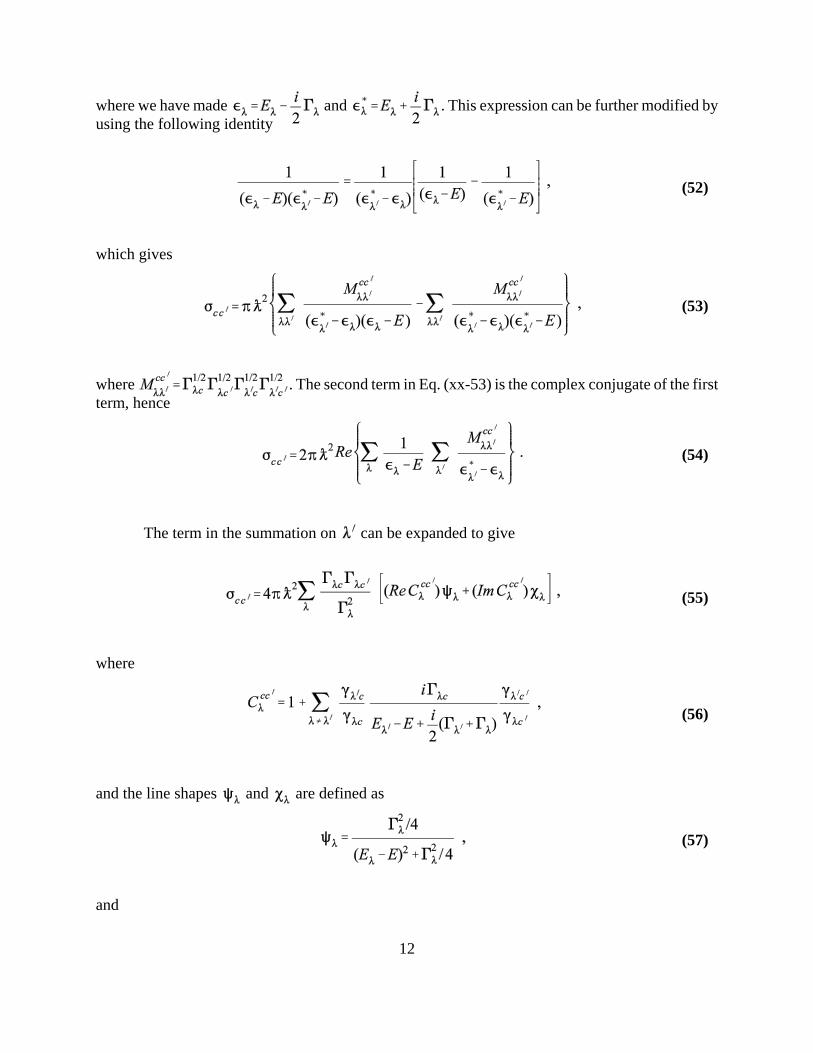
where we have made and . This expression can be further modified byusing the following identity

which gives

where . The second term in Eq. (xx-53) is the complex conjugate of the firstterm, hence

The term in the summation on can be expanded to give

where

and the line shapes and are defined as

and

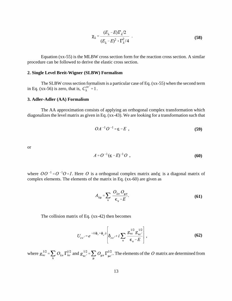
13

(58)

(59)

(60)

(61)

(62)

Equation (xx-55) is the MLBW cross section form for the reaction cross section. A similarprocedure can be followed to derive the elastic cross section.

2. Single Level Breit-Wigner (SLBW) Formalism

The SLBW cross section formalism is a particular case of Eq. (xx-55) when the second termin Eq. (xx-56) is zero, that is, .

3. Adler-Adler (AA) Formalism

The AA approximation consists of applying an orthogonal complex transformation whichdiagonalizes the level matrix as given in Eq. (xx-43). We are looking for a transformation such that

or

where . Here is a orthogonal complex matrix and is a diagonal matrix ofcomplex elements. The elements of the matrix in Eq. (xx-60) are given as

The collision matrix of Eq. (xx-42) then becomes

where and . The elements of the matrix are determined from

14

(63)

(64)

(65)

(66)

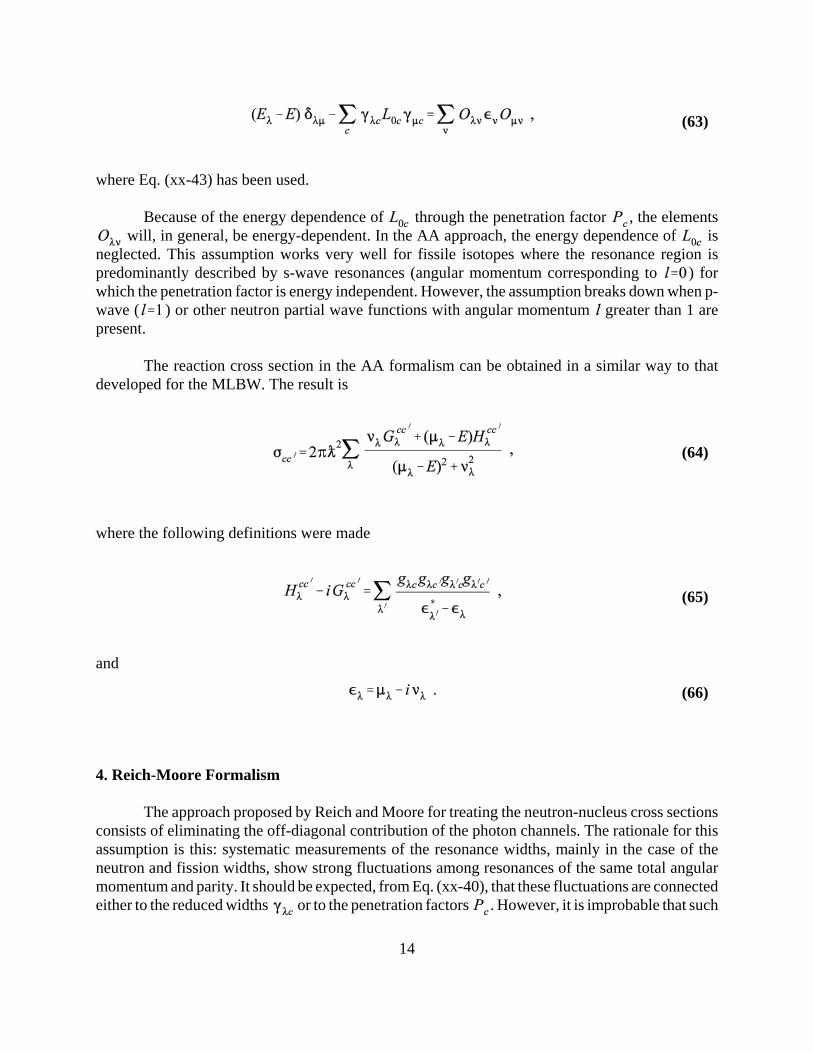
where Eq. (xx-43) has been used.

Because of the energy dependence of through the penetration factor , the elements will, in general, be energy-dependent. In the AA approach, the energy dependence of is

neglected. This assumption works very well for fissile isotopes where the resonance region ispredominantly described by s-wave resonances (angular momentum corresponding to ) forwhich the penetration factor is energy independent. However, the assumption breaks down when p-wave ( ) or other neutron partial wave functions with angular momentum greater than 1 arepresent.

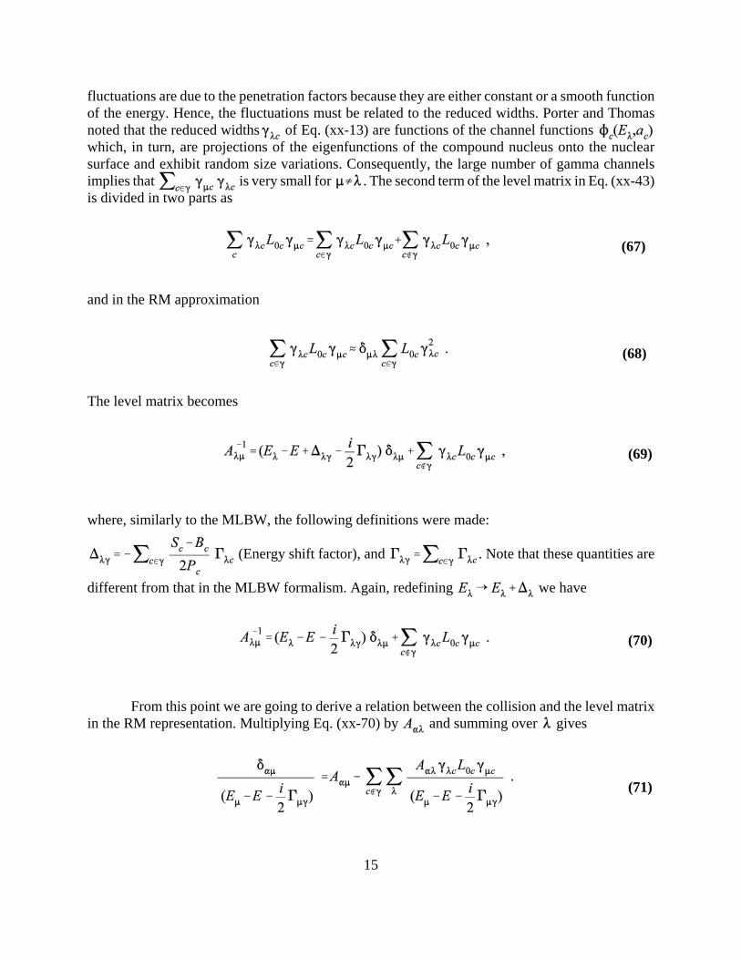
The reaction cross section in the AA formalism can be obtained in a similar way to thatdeveloped for the MLBW. The result is

where the following definitions were made

and

4. Reich-Moore Formalism

The approach proposed by Reich and Moore for treating the neutron-nucleus cross sectionsconsists of eliminating the off-diagonal contribution of the photon channels. The rationale for thisassumption is this: systematic measurements of the resonance widths, mainly in the case of theneutron and fission widths, show strong fluctuations among resonances of the same total angularmomentum and parity. It should be expected, from Eq. (xx-40), that these fluctuations are connectedeither to the reduced widths or to the penetration factors . However, it is improbable that such

15

(67)

(68)

(69)

(70)

(71)

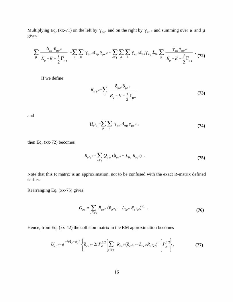
fluctuations are due to the penetration factors because they are either constant or a smooth functionof the energy. Hence, the fluctuations must be related to the reduced widths. Porter and Thomasnoted that the reduced widths of Eq. (xx-13) are functions of the channel functions which, in turn, are projections of the eigenfunctions of the compound nucleus onto the nuclearsurface and exhibit random size variations. Consequently, the large number of gamma channelsimplies that is very small for . The second term of the level matrix in Eq. (xx-43)is divided in two parts as

and in the RM approximation

The level matrix becomes

where, similarly to the MLBW, the following definitions were made:

(Energy shift factor), and . Note that these quantities are

different from that in the MLBW formalism. Again, redefining we have

From this point we are going to derive a relation between the collision and the level matrixin the RM representation. Multiplying Eq. (xx-70) by and summing over gives

16

(72)

(73)

(74)

(75)

(76)

(77)

Multiplying Eq. (xx-71) on the left by and on the right by and summing over and gives

If we define

and

then Eq. (xx-72) becomes

Note that this R matrix is an approximation, not to be confused with the exact R-matrix definedearlier.

Rearranging Eq. (xx-75) gives

Hence, from Eq. (xx-42) the collision matrix in the RM approximation becomes

17

(78)

(79)

(80)

(81)

(82)

(83)

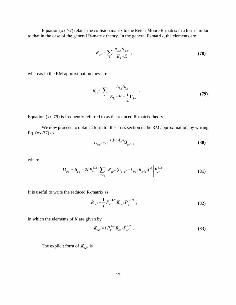
Equation (xx-77) relates the collision matrix to the Reich-Moore R-matrix in a form similarto that in the case of the general R-matrix theory. In the general R-matrix, the elements are

whereas in the RM approximation they are

Equation (xx-79) is frequently referred to as the reduced R-matrix theory.

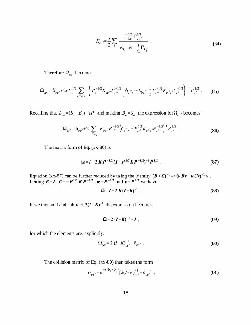
We now proceed to obtain a form for the cross section in the RM approximation, by writingEq. (xx-77) as

where

It is useful to write the reduced R-matrix as

in which the elements of K are given by

The explicit form of is

18

(84)

(85)

(86)

(87)

(88)

(89)

(90)

(91)

Therefore becomes

Recalling that and making , the expression for becomes

The matrix form of Eq. (xx-86) is

Equation (xx-87) can be further reduced by using the identity .Letting , , and we have

If we then add and subtract the expression becomes,

for which the elements are, explicitly,

The collision matrix of Eq. (xx-80) then takes the form

19

(92)

(93)

(94)

(95)

(96)

(97)

(98)

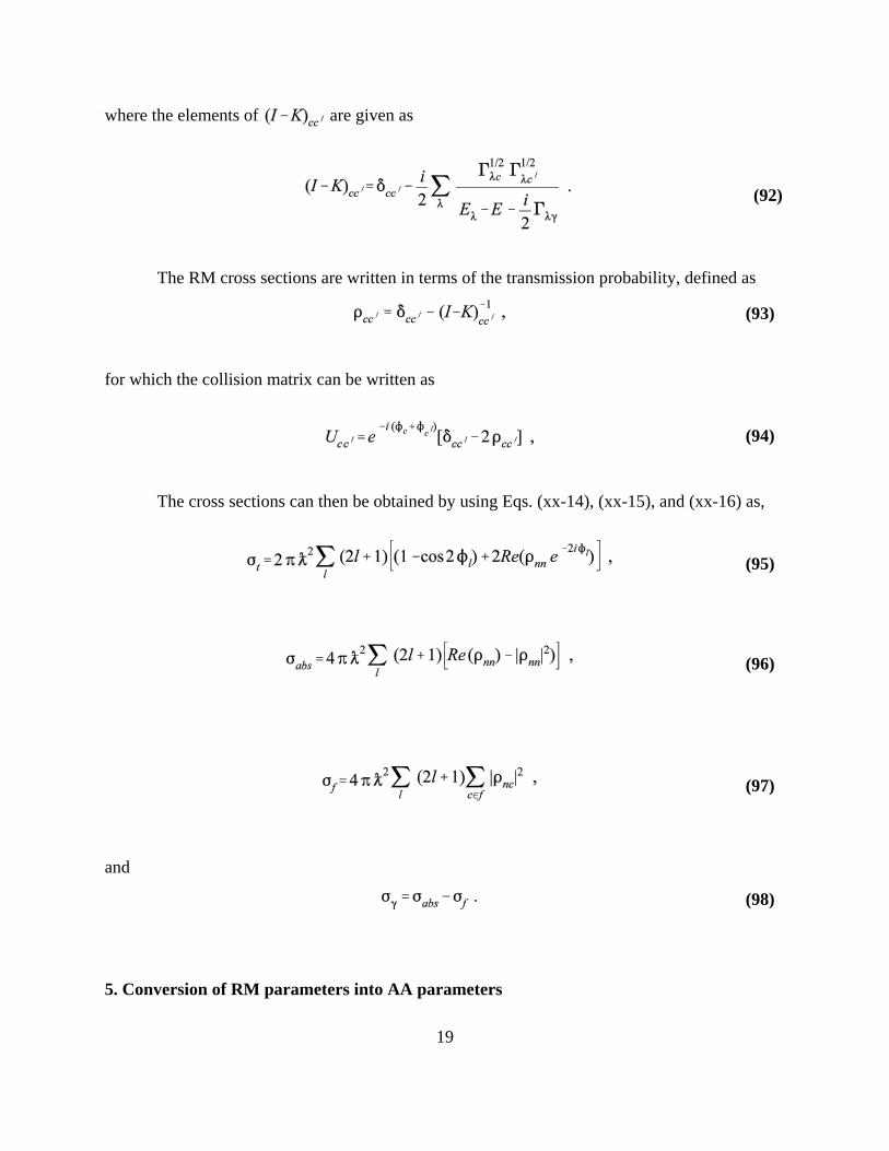
where the elements of are given as

The RM cross sections are written in terms of the transmission probability, defined as

for which the collision matrix can be written as

The cross sections can then be obtained by using Eqs. (xx-14), (xx-15), and (xx-16) as,

and

5. Conversion of RM parameters into AA parameters

20

(99)

(100)

(101)

(102)

(103)

(104)

A procedure to convert RM parameters into an equivalent set of AA parameters wasdeveloped by DeSaussure and Perez. Their approach consisted of writing the RM transmissionprobabilities and as the ratio of polynomials in energy; these polynomials can then beexpressed in terms of partial fraction expansions by matching the AA cross sections as:

and

where

and .

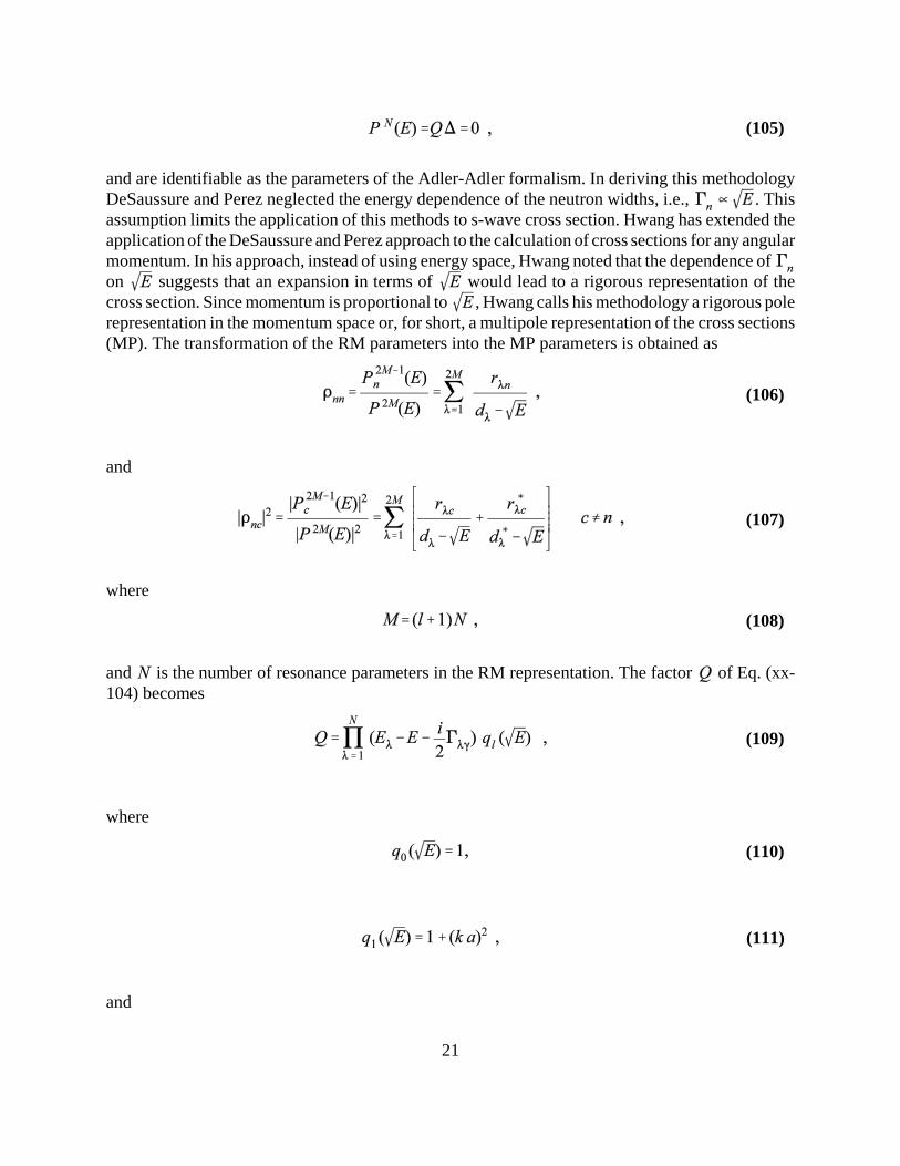
Equations (xx-99) and (xx-100) have poles which are roots of the equation

21

(105)

(106)

(107)

(108)

(109)

(110)

(111)

and are identifiable as the parameters of the Adler-Adler formalism. In deriving this methodologyDeSaussure and Perez neglected the energy dependence of the neutron widths, i.e., . Thisassumption limits the application of this methods to s-wave cross section. Hwang has extended theapplication of the DeSaussure and Perez approach to the calculation of cross sections for any angularmomentum. In his approach, instead of using energy space, Hwang noted that the dependence of on suggests that an expansion in terms of would lead to a rigorous representation of thecross section. Since momentum is proportional to , Hwang calls his methodology a rigorous polerepresentation in the momentum space or, for short, a multipole representation of the cross sections(MP). The transformation of the RM parameters into the MP parameters is obtained as

and

where

and is the number of resonance parameters in the RM representation. The factor of Eq. (xx-104) becomes

where

and

22

(112)

(113)

(114)

(115)

Doppler Broadening and Effective Cross Sections

The Doppler broadening of cross sections is a well-known effect which is caused by the motionof the atoms of the target nuclei. Since the target nuclei are not at rest in the laboratory system,the neutron-nucleus cross section will depend on the relative speed of the neutron and thenucleus. The effective cross section for mono-energetic neutrons of mass m and energy E(laboratory velocity v) is given by the number of neutrons per unit volume, multiplied by thenumber of target nuclei per unit volume, times the probability that a reaction will occur per unittime at an energy equivalent to the relative velocity | v! W |, integrated over all values of W, thevelocity of the nucleus. The relation between the cross section measured in the laboratory andthe effective cross section is

where is the effective or Doppler-broadened cross section for incident particles withspeed v [laboratory energy mv2/2]. The distribution of velocities of the target nuclei is describedby . A major issue is the choice of the appropriate velocity distribution function of thetarget nuclei. Let us now assume that the target nuclei have the same velocity distribution as theatoms of an ideal gas; i.e. the Maxwell-Boltzmann distribution,

where M is the nuclear mass and kT the gas temperature in energy units. Combining Eqs. (xx-113) and (xx-114) gives

Note that, from the above definitions, a 1/v cross section remains unchanged.

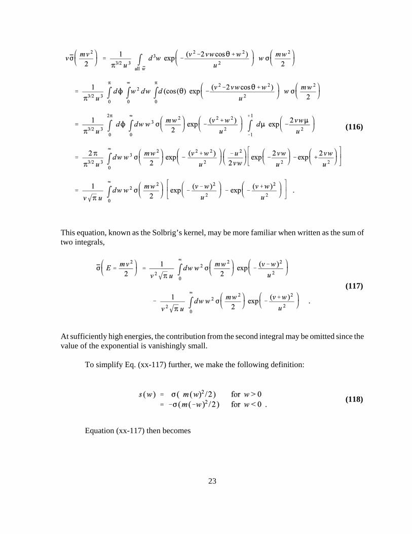
Changing the integration variable from and choosing sphericalcoordinates simplifies the integral to the following:

23

(116)

(117)

(118)

This equation, known as the Solbrig’s kernel, may be more familiar when written as the sum oftwo integrals,

At sufficiently high energies, the contribution from the second integral may be omitted since thevalue of the exponential is vanishingly small.

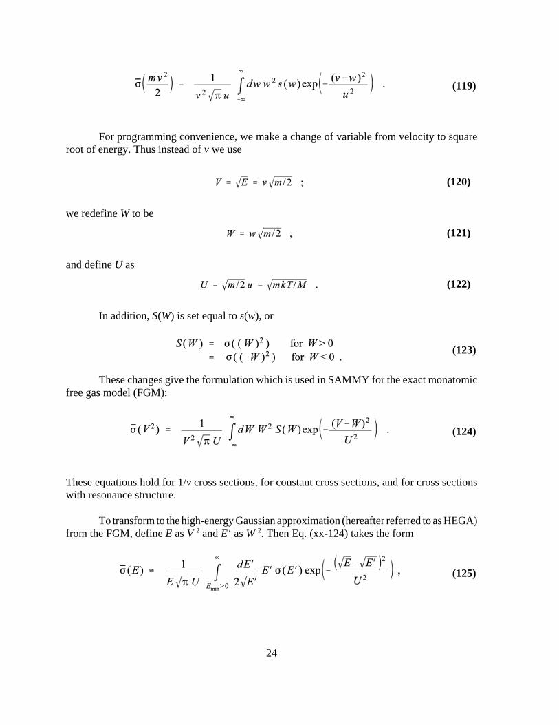
To simplify Eq. (xx-117) further, we make the following definition:

Equation (xx-117) then becomes

24

(119)

(120)

(121)

(122)

(123)

(124)

(125)

For programming convenience, we make a change of variable from velocity to squareroot of energy. Thus instead of v we use

we redefine W to be

and define U as

In addition, S(W) is set equal to s(w), or

These changes give the formulation which is used in SAMMY for the exact monatomicfree gas model (FGM):

These equations hold for 1/v cross sections, for constant cross sections, and for cross sectionswith resonance structure.

To transform to the high-energy Gaussian approximation (hereafter referred to as HEGA)from the FGM, define E as V 2 and EN as W 2. Then Eq. (xx-124) takes the form

25

(126)

(127)

(128)

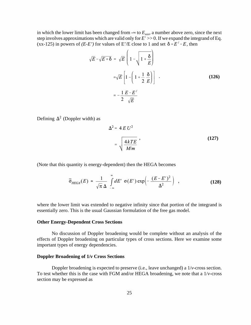
in which the lower limit has been changed from -4 to Emin, a number above zero, since the nextstep involves approximations which are valid only for EN >> 0. If we expand the integrand of Eq.(xx-125) in powers of (E-E’) for values of E’/E close to 1 and set , then

Defining (Doppler width) as

(Note that this quantity is energy-dependent) then the HEGA becomes

where the lower limit was extended to negative infinity since that portion of the integrand isessentially zero. This is the usual Gaussian formulation of the free gas model.

Other Energy-Dependent Cross Sections

No discussion of Doppler broadening would be complete without an analysis of theeffects of Doppler broadening on particular types of cross sections. Here we examine someimportant types of energy dependencies.

Doppler Broadening of 1/v Cross Sections

Doppler broadening is expected to preserve (i.e., leave unchanged) a 1/v-cross section.To test whether this is the case with FGM and/or HEGA broadening, we note that a 1/v-crosssection may be expressed as

26

(129)

(130)

(131)

(132)

where the subscript “0” denotes constants. To evaluate the FGM with this type of cross section,note that our function S of Eq. (xx-123), combined with Eq. (xx-129), gives

From Eq. (xx-11) the FGM-broadened form of the 1/v cross section is therefore

i.e., in the exact same mathematical form as the original of Eq. (xx-129). In other words, a 1/vcross section is conserved under Doppler broadening with the free gas model.

That is not the case for HEGA broadening. With the HEGA from Eq. (xx-128), theDoppler-broadened 1/v cross section takes the form

which is not readily integrable analytically. What is clear is that the result is not 1/v.

Doppler Broadening of a Constant Cross Section

In contrast to the 1/v cross section, a constant cross section is not conserved underDoppler broadening. That it is true experimentally can be seen by examining very low energycapture cross sections, for which the unbroadened cross section is constant (which can be shown

27

(133)

(134)

(135)

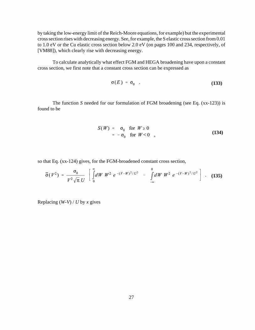
by taking the low-energy limit of the Reich-Moore equations, for example) but the experimentalcross section rises with decreasing energy. See, for example, the S elastic cross section from 0.01to 1.0 eV or the Cu elastic cross section below 2.0 eV (on pages 100 and 234, respectively, of[VM88]), which clearly rise with decreasing energy.

To calculate analytically what effect FGM and HEGA broadening have upon a constantcross section, we first note that a constant cross section can be expressed as

The function S needed for our formulation of FGM broadening (see Eq. (xx-123)) isfound to be

so that Eq. (xx-124) gives, for the FGM-broadened constant cross section,

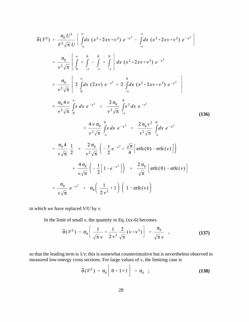
Replacing (W-V) / U by x gives

28

(136)

(137)

(138)

in which we have replaced V/U by v.

In the limit of small v, the quantity in Eq. (xx-6) becomes

so that the leading term is 1/v; this is somewhat counterintuitive but is nevertheless observed inmeasured low-energy cross sections. For large values of v, the limiting case is

29

(139)

(140)

(141)

(142)

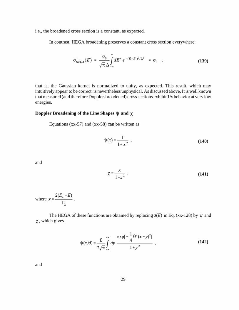
i.e., the broadened cross section is a constant, as expected.

In contrast, HEGA broadening preserves a constant cross section everywhere:

that is, the Gaussian kernel is normalized to unity, as expected. This result, which mayintuitively appear to be correct, is nevertheless unphysical. As discussed above, It is well knownthat measured (and therefore Doppler-broadened) cross sections exhibit 1/v behavior at very lowenergies.

Doppler Broadening of the Line Shapes and

Equations (xx-57) and (xx-58) can be written as

and

where .

The HEGA of these functions are obtained by replacing in Eq. (xx-128) by and, which gives

and

30

(143)

where .

MIT OpenCourseWarehttp://ocw.mit.edu

22.106 Neutron Interactions and Applications Spring 2010

For information about citing these materials or our Terms of Use, visit: http://ocw.mit.edu/terms.