Bridge Girder Drag Coefficients and Wind-related Bracing Recommendations
249
1 BRIDGE GIRDER DRAG COEFFICIENTS AND WIND-RELATED BRACING RECOMMENDATIONS By ZACHARY HARPER A THESIS PRESENTED TO THE GRADUATE SCHOOL OF THE UNIVERSITY OF FLORIDA IN PARTIAL FULFILLMENT OF THE REQUIREMENTS FOR THE DEGREE OF MASTER OF SCIENCE UNIVERSITY OF FLORIDA 2013
-
Upload
pablo-augusto-krahl -
Category
Documents
-
view
239 -
download
1
description
Considerações de açoes de vento em pontes
Transcript of Bridge Girder Drag Coefficients and Wind-related Bracing Recommendations

1
BRIDGE GIRDER DRAG COEFFICIENTS AND WIND-RELATED BRACING
RECOMMENDATIONS
By
ZACHARY HARPER
A THESIS PRESENTED TO THE GRADUATE SCHOOL
OF THE UNIVERSITY OF FLORIDA IN PARTIAL FULFILLMENT
OF THE REQUIREMENTS FOR THE DEGREE OF
MASTER OF SCIENCE
UNIVERSITY OF FLORIDA
2013

2
© 2013 Zachary Harper

3
ACKNOWLEDGMENTS
I would not have been able to complete this thesis and the associated research, without
the continual guidance and support of my advisor, Dr. Gary Consolazio. With his deep
engineering knowledge, attention to detail, and commitment to excellence, he has played a far
larger part than any other individual in making me the engineer and researcher I am today.
Dr. Kurt Gurley’s wind engineering expertise has been invaluable to this research. I
would also like to thank Dr. H.R. (Trey) Hamilton and Dr. Ron Cook for serving on my
supervisory committee.
In addition to the school’s excellent faculty, I would like to acknowledge the support,
advice, and friendship of the fellow engineering graduate students with whom I have shared an
office, including Dr. Michael Davidson, Daniel Getter, Megan Beery, Natassia Brenkus, John
Wilkes, and Sam Edwards. The past few years would have been much more difficult (and much
less fun) without them. In particular, I would like to highlight the contribution of Daniel Getter to
my personal and professional development. Daniel is much too generous with his time, and has
always been willing to offer his vast technical knowledge and sage advice. Additionally, I would
like to thank Megan Beery, for her willingness to discuss the details of her research (upon which
my own is partly based), and Sam Edwards for his assistance with the preparation of this
manuscript.
Finally, and most importantly, I want to thank my parents, Bill and Patricia Harper. None
of what I have accomplished would have been possible without their 26 years of unwavering
patience, love, and support.
4
TABLE OF CONTENTS
page
ACKNOWLEDGMENTS ...............................................................................................................3
LIST OF TABLES ...........................................................................................................................8
LIST OF FIGURES .........................................................................................................................9
ABSTRACT ...................................................................................................................................16
CHAPTER
1 INTRODUCTION ..................................................................................................................18
1.1 Introduction ...................................................................................................................18
1.2 Objectives ......................................................................................................................19 1.3 Scope of Work...............................................................................................................19
2 PHYSICAL DESCRIPTION OF BRIDGES DURING CONSTRUCTION .........................22
2.1 Introduction ...................................................................................................................22 2.2 Geometric Parameters ...................................................................................................22
2.3 Bearing Pads .................................................................................................................23 2.4 Sources of Lateral Instability ........................................................................................23
2.5 Lateral Wind Loads .......................................................................................................25
2.6 Temporary Bracing .......................................................................................................25
2.6.1 Anchor Bracing .................................................................................................25 2.6.2 Girder-to-Girder Bracing ..................................................................................26
3 BACKGROUND ON DRAG COEFFICIENTS ....................................................................34
3.1 Introduction ...................................................................................................................34
3.2 Dimensionless Aerodynamic Coefficients ....................................................................34 3.3 Terminology Related to Aerodynamic Coefficients .....................................................37 3.4 Current Wind Design Practice in Florida ......................................................................38 3.5 Literature Review: Drag Coefficients for Bridge Girders.............................................41
4 WIND TUNNEL TESTING ...................................................................................................49
4.1 Introduction ...................................................................................................................49 4.2 Testing Configurations ..................................................................................................49
4.2.1 Number of Girders ............................................................................................50 4.2.2 Spacing ..............................................................................................................50 4.2.3 Cross-Slope .......................................................................................................51 4.2.4 Wind Angle .......................................................................................................51
4.3 Testing Procedure..........................................................................................................52
5
5 WIND TUNNEL RESULTS AND ANALYSIS ....................................................................57
5.1 Introduction ...................................................................................................................57 5.2 Aerodynamic Coefficients for Individual Girders ........................................................57 5.3 Examination of Shielding Trends .................................................................................59
5.4 Effective Drag Coefficient ............................................................................................61 5.5 Proposed Wind Loads for Design .................................................................................64 5.6 Proposed Procedure for Calculation of Brace Forces ...................................................66
6 BEARING PADS ...................................................................................................................82
6.1 Introduction ...................................................................................................................82
6.2 Behavior of Pads in Compression .................................................................................83 6.3 Behavior of Pads in Roll Rotation ................................................................................85
6.4 Calculation of Shear and Torsion Stiffness ...................................................................86 6.5 Calculation of Axial Stiffness .......................................................................................86
6.5.1 Stiffness of Neoprene Layers ............................................................................87 6.5.2 Model Dimensions and Meshing ......................................................................87
6.5.3 Loading and Boundary Conditions ...................................................................88 6.5.4 Material Model ..................................................................................................88
6.5.5 Experimental Validation ...................................................................................90 6.6 Calculation of Nonlinear Roll Stiffness Curves ............................................................90
6.6.1 Grillage Model ..................................................................................................90
6.6.2 Spring Stiffness Distribution in Grillage Model ...............................................91 6.6.3 Incorporating Girder Slope ...............................................................................92
6.7 Simplified Method for Calculating Axial Stiffness and Instantaneous Roll
Stiffnesses .....................................................................................................................93
6.7.1 Axial Stiffness ...................................................................................................94 6.7.2 Basic Derivation of Instantaneous Roll Stiffness of a Continuous Grillage .....96
6.7.3 Incorporating Girder Slope ...............................................................................97
7 MODEL DEVELOPMENT ..................................................................................................114
7.1 Introduction .................................................................................................................114 7.2 Modeling of Bridge Girders ........................................................................................115 7.3 Modeling of End Supports ..........................................................................................117
7.3.1 Pad Selection ...................................................................................................117 7.3.2 Axial Load Selection .......................................................................................118
7.3.3 Girder Slope Selection ....................................................................................118
7.4 Modeling of Braces and Anchors ................................................................................119
7.5 Loads ...........................................................................................................................121 7.6 Modified Southwell Buckling Analysis ......................................................................122
8 PARAMETRIC STUDY OF INDIVIDUAL BRIDGE GIRDERS .....................................132
8.1 Introduction .................................................................................................................132 8.2 Selection of Parameters ...............................................................................................132
6
8.3 Results .........................................................................................................................134
8.3.1 Wind Capacity of a Single Unanchored Girder ..............................................135 8.3.2 Wind Capacity of a Single Anchored Girder ..................................................136
9 PARAMETRIC STUDY OF BRACED MULTI-GIRDER SYSTEMS ..............................145
9.1 Preliminary Sensitivity Studies ...................................................................................145 9.1.1 Strut Braces .....................................................................................................145 9.1.2 Moment-Resisting Braces ...............................................................................146
9.2 Modeling of Bridge Skew and Wind Load .................................................................147 9.3 Selection of Parameters for Strut Brace Parametric Study .........................................148
9.4 Results of Strut Brace Parametric Study .....................................................................149 9.4.1 System Capacity of Unanchored Two-Girder System in Zero Wind .............151 9.4.2 System Capacity Increase from Inclusion of Anchor .....................................151
9.4.3 System Capacity Reduction from Erection of Additional Girders..................152 9.4.4 System Capacity Reduction from Inclusion of Wind Load ............................153 9.4.5 Consideration of Skew ....................................................................................155
9.5 Stiffness of Moment-Resisting Braces ........................................................................156 9.6 Selection of Parameters for Moment-Resisting Brace Parametric Study ...................158
9.7 Results of Moment-Resisting Brace Parametric Study ...............................................159 9.7.1 System Capacity Increase from Inclusion of Moment-Resisting End
Braces ..............................................................................................................160
9.7.2 System Capacity Increase from Installation of Braces at Interior Points........161 9.7.3 System Capacity Reduction from Inclusion of Wind Load ............................162
9.7.4 Consideration of Skew ....................................................................................164 9.8 Incorporation of Aerodynamic Lift .............................................................................164
10 CONCLUSIONS AND RECOMMENDATIONS ...............................................................186
10.2 Drag Coefficients ........................................................................................................186
10.3 Individual Unbraced Florida-I Beams .........................................................................188 10.4 Braced Systems of Multiple Florida-I Beams .............................................................189
10.5 Future Research ...........................................................................................................190
APPENDIX
A DIMENSIONED DRAWINGS OF WIND TUNNEL TEST CONFIGURATIONS ..........193
B TABULATED RESULTS FROM WIND TUNNEL TESTS ..............................................202
C CROSS-SECTIONAL PROPERTIES OF FLORIDA-I BEAMS ........................................220
D PROPERTIES OF FLORIDA BEARING PADS ................................................................224
E PLOTS OF CAPACITY PREDICTION EQUATIONS ......................................................236
LIST OF REFERENCES .............................................................................................................246

7
BIOGRAPHICAL SKETCH .......................................................................................................249
8
LIST OF TABLES
Table page
3-1 Summary of aerodynamic coefficients ..............................................................................45
3-2 Pressure coefficients in FDOT Structures Design Guide (SDG) .......................................45
3-3 Drag coefficients (CD) of thin-walled I-shapes .................................................................45
4-1 Testing configurations .......................................................................................................54
4-2 Wind tunnel test scaling .....................................................................................................54
5-1 Aerodynamic coefficients of bridge girder cross-sectional shapes ....................................69
5-2 Extreme combinations of tested wind angle and cross-slope ............................................69
8-1 Parameter values used in parametric study for each FIB cross-section ...........................139
8-2 Range of allowable span lengths for FIBs .......................................................................140
9-1 Parameter values used in strut brace parametric study ....................................................168
9-2 Girder offset lengths in model for each skew angle ........................................................168
9-3 Parameter values used in moment-resisting brace parametric study ...............................169
9-4 Empirically-determined values of ω for different numbers of interior braces ................169
9-5 Selfweight (wsw) of each FIB cross-sectional shape (from FDOT, 2012) ......................169
B-1 Meaning of letters in configuration IDs ...........................................................................202
C-1 Definitions of cross-sectional properties required for use of a warping beam element...222
C-2 Cross-sectional properties of Florida-I Beams ................................................................222
D-1 Bearing pad dimensions and computed stiffnesses ..........................................................225
9
LIST OF FIGURES
Figure page
1-1 Prestressed concrete girders braced together for stability..................................................21
2-1 Girder system .....................................................................................................................27
2-2 Definition of grade (side view) ..........................................................................................27
2-3 Definition of cross-slope (section view) ............................................................................27
2-4 Definition of skew (top view) ............................................................................................28
2-5 Definition of camber (elevation view) ...............................................................................28
2-6 Definition of sweep (plan view) ........................................................................................28
2-7 Rollover instability of girder ..............................................................................................28
2-8 Lateral-torsional instability of girder .................................................................................29
2-9 Increase in secondary effects due to higher application of vertical load ...........................29
2-10 Effects of wind on stability of girder. ................................................................................30
2-11 Common anchor types. ......................................................................................................31
2-12 Chain braces on Florida Bulb-Tee during transportation ..................................................32
2-13 Perpendicular brace placement on skewed bridge .............................................................32
2-14 Common brace types..........................................................................................................33
3-1 Two-dimensional bridge girder cross-section with in-plane line loads .............................45
3-2 Definition of CD, CL, CSD, and CSL ................................................................................46
3-3 Center of pressure of a bridge girder .................................................................................46
3-4 Definition of CT and CPT ..................................................................................................46
3-5 Velocity pressure exposure coefficient used by FDOT .....................................................47
3-6 Examples of I-shaped girders (steel plate girders and Florida-I Beams) for which CP
= 2.2 (per FDOT, 2012e) ...................................................................................................47
3-7 Example open top box girder cross-section for which CP = 1.5 (per FDOT, 2012e) .......47
10
3-8 Drag coefficients for rectangular sections with various width-to-depth ratios ..................48
3-9 Drag coefficients for plate girder shapes and rectangles with various width-to-depth
ratios ...................................................................................................................................48
4-1 Girder cross-sections used in study (drawn to scale) .........................................................54
4-2 Girder groupings investigated in study ..............................................................................55
4-3 Parameters definitions for each testing configuration .......................................................55
4-4 Wind angle sign convention...............................................................................................55
4-5 Equivalence between wind angle and cross-slope for box girders ....................................56
5-1 Effect of wind angle on individual girder drag coefficients (CD) .....................................69
5-2 Effect of wind angle on individual girder lift coefficients (CL) ........................................70
5-3 Effect of wind angle on individual torque coefficients (CT) .............................................70
5-4 Drag coefficients of WF Plate girders in 5-girder configurations (0° Wind) ....................71
5-5 Effect of adding additional girders ....................................................................................71
5-6 Effect of wind angle on CD ...............................................................................................72
5-7 Interaction between wind angle and cross-slope. ..............................................................72
5-8 Ten (10) girder models tested at wind angles producing maximum shielding ..................73
5-9 Ten (10) girder models tested at wind angles producing minimum shielding ...................73
5-10 Effect of wind angle on two (2) Box girder system drag coefficients (CD) ......................74
5-11 Lift coefficients on all I-shaped girder test configurations (plate girders and FIBs) .........74
5-12 Torque coefficients on all I-shaped girder test configurations (plate girders and FIBs) ...75
5-13 Transformation of CT to CPT. ...........................................................................................76
5-14 Moment load expressed as equivalent drag force. .............................................................76
5-15 Comparison between maximum CD and maximum CD,eff ..............................................77
5-16 Proposed design loads for plate girders .............................................................................78
5-17 Proposed design loads for FIBs .........................................................................................78
11
5-18 Representation of positive and negative drag loads as a combined compression load ......79
5-19 Proposed brace force design loads for plate girders ..........................................................79
5-20 Proposed brace force design loads for FIBs ......................................................................80
5-21 Simplified brace force analysis. .........................................................................................81
6-1 Location and structure of neoprene bearing pads ............................................................101
6-2 Bulging of neoprene layers under compression. ..............................................................102
6-3 Distribution of reaction force under bearing pad subjected to uniform axial load ..........103
6-4 Behavior of bearing pads during girder rollover. .............................................................104
6-5 Dimensions of a bearing pad ............................................................................................104
6-6 Axial stiffness of pad as individual layer stiffnesses combined in series ........................105
6-7 Finite element model of elastomer layer ..........................................................................105
6-8 Validation of neo-Hookean material model. ....................................................................106
6-9 Simplified grillage model of a bearing pad......................................................................107
6-10 Standard FDOT bearing pads used for experimental verification ...................................108
6-11 Distribution of stiffness to grillage springs. .....................................................................109
6-12 Comparison of experimentally measured bearing pad roll stiffnesses and roll
stiffnesses predicted by the proposed computation method ............................................110
6-13 Bearing pad slope. ............................................................................................................111
6-14 Comparison of experimentally measured bearing pad roll stiffnesses and roll
stiffnesses predicted by the proposed computation method with non-zero slope. ...........112
6-15 Coordinate system of continuous grillage (plan view). ...................................................112
6-16 Continuous grillage with imposed differential angle .......................................................113
6-17 Comparison between Equation 6-28 and the square root approximation ........................113
7-1 Finite element model of a single FIB (isometric view) ...................................................126
7-2 Representation of sweep in FIB model (plan view).........................................................126
7-3 Representation of camber in FIB model (elevation view) ...............................................126
12
7-4 Bearing pad stiffness springs in FIB model (isometric view) ..........................................127
7-5 Representation of brace configurations in FIB system models. ......................................128
7-6 Calculation of rotational stiffness of anchor ....................................................................129
7-7 Longitudinally-inclined anchors on skewed bridges .......................................................129
7-8 Representation of wind load in structural models............................................................129
7-9 Southwell method for determining critical buckling load (β). .........................................130
7-10 Southwell analysis of non-hyperbolic displacement–load data obtained from a large-
displacement structural analysis ......................................................................................131
7-11 Determination of buckling capacity using modified Southwell approach .......................131
8-1 Summary of single-girder wind-load parametric study results ........................................140
8-2 Wind capacities of unanchored FIBs at various span lengths..........................................141
8-3 Wind capacity of an unanchored girder as predicted by Equation 8-2 ............................141
8-4 Wind capacity of an unanchored girder as predicted by simplified Equation 8-3 ...........142
8-5 Comparison of basic and simplified unanchored girder wind capacity equations,
Equations 8-2 and 8-3, respectively .................................................................................142
8-6 Effect of anchor rotational stiffness on wind capacity for 84″ FIB .................................143
8-7 Rejection of artificially-inflated wind capacity data points (84″ FIB) ............................143
8-8 Anchor stiffness coefficient Equation 8-5 compared to parametric study results ...........144
8-9 Comparison of wind capacity results computed using the combination of Equations
8-2 and 8-6 versus corresponding parametric study results .............................................144
9-1 Examples of strut bracing ................................................................................................170
9-2 Collapse mechanism possible with strut bracing .............................................................170
9-3 Examples of moment-resisting braces. ............................................................................170
9-4 Effect of bridge skew on wind loading of braced 3-girder system (plan view). ..............171
9-5 Summary of strut brace parametric study results .............................................................171
9-6 System capacities of unanchored two-girder strut-braced systems in zero wind at
various span lengths .........................................................................................................172
13
9-7 System capacity of an unanchored strut-braced two-girder system in zero wind as
predicted by Equation 9-2 ................................................................................................172
9-8 Effect of anchor stiffness on capacity of 96″ FIB system................................................173
9-10 Relative error of system capacity values predicted by Equation 9-4 ...............................174
9-11 Relative error of system capacity values predicted by Equation 9-6 ...............................174
9-12 Effect of average wind pressure on system capacity of 78″ 2-FIB system with anchor
stiffness of 1600 kip-ft/rad ...............................................................................................175
9-13 Approximate linear relationship between system capacity and square root of average
wind pressure ...................................................................................................................175
9-14 Quadratic surface (Equation 9-9) fitted to wind pressure coefficient values...................176
9-15 Absolute error of system capacity values predicted by Equation 9-10 ............................176
9-16 Absolute error of system capacity values predicted by Equation 9-10 for strut-braced
systems, including systems with non-zero skew angles ..................................................177
9-17 Brace designs in brace inventory (each implemented at three different spacings and
three different FIB depths) ...............................................................................................178
9-18 Model used to compute effective stiffness of brace configurations ................................178
9-19 Reference brace configuration used in parametric studies ..............................................179
9-20 Cross-section of 36″ FIB..................................................................................................179
9-21 Stiffness of every brace in brace inventory......................................................................179
9-22 Stiffness of every X-brace in brace inventory .................................................................180
9-23 Summary of moment-resisting brace parametric study results ........................................180
9-24 Equation 9-12 (β) compared to parametric study results .................................................181
9-25 Equation 9-12 (β) compared to parametric study results .................................................181
9-26 Relative error of system capacity values predicted by Equation 9-13 .............................182
9-27 Relative error of system capacity values predicted by Equation 9-14 .............................182
9-28 Approximate linear relationship between system capacity and square root of average
wind pressure ...................................................................................................................183
14
9-29 Quadratic surface (Equation 9-16) fitted to wind pressure coefficient values and
adjusted to produce conservative results in 95% of cases ...............................................184
9-30 Absolute error of system capacity values predicted by Equation 9-17 for moment-
resisting braced systems ...................................................................................................184
9-31 Absolute error of system capacity values predicted by Equation 9-17 for moment-
resisting braced systems, including systems with non-zero skew angles ........................185
10-1 Girder cross-sectional shapes tested in the wind tunnel ..................................................191
10-2 Recommended design wind loads for systems of adjacent girders ..................................191
10-3 Recommended structural analysis model for use in determining brace forces. ...............192
C-1 Coordinate system used in the calculation of cross-sectional properties .........................223
D-1 Bearing pad dimensions and variables .............................................................................225
E-1 Prediction of system capacity for 2-girder, unanchored strut-braced systems in 0-psf
wind (Equation 9-10) .......................................................................................................236
E-2 Prediction of system capacity for 2-girder, unanchored strut-braced systems in 40-psf
wind (Equation 9-10) .......................................................................................................237
E-3 Prediction of system capacity for 2-girder, unanchored strut-braced systems in 80-psf
wind (Equation 9-10) .......................................................................................................237
E-4 Prediction of system capacity for 2-girder, unanchored strut-braced systems in 120-
psf wind (Equation 9-10) .................................................................................................238
E-5 Prediction of system capacity for 2-girder, unanchored strut-braced systems in 160-
psf wind (Equation 9-10) .................................................................................................238
E-6 Prediction of system capacity for end-braced systems in 0-psf wind with moment-
resisting braces with kbrace = 15,000 kip-ft/rad (Equation 9-17) ...................................239
E-7 Prediction of system capacity for end-braced systems in 0-psf wind with moment-
resisting braces with kbrace = 200,000 kip-ft/rad (Equation 9-17) .................................239
E-8 Prediction of system capacity for end-braced systems in 0-psf wind with moment-
resisting braces with kbrace = 400,000 kip-ft/rad (Equation 9-17) .................................240
E-9 Prediction of system capacity for end-braced systems in 0-psf wind with moment-
resisting braces with kbrace = 600,000 kip-ft/rad (Equation 9-17) .................................240
E-10 Prediction of system capacity for systems in 0-psf wind with moment-resisting
braces (kbrace = 200,000 kip-ft/rad) with no interior brace points (Equation 9-17) .......241
15
E-11 Prediction of system capacity for systems in 0-psf wind with moment-resisting
braces (kbrace = 200,000 kip-ft/rad) with 1 interior brace point (Equation 9-17) ..........241
E-12 Prediction of system capacity for systems in 0-psf wind with moment-resisting
braces (kbrace = 200,000 kip-ft/rad) with 2 interior brace points (Equation 9-17) .........242
E-13 Prediction of system capacity for systems in 0-psf wind with moment-resisting
braces (kbrace = 200,000 kip-ft/rad) with 3 interior brace points (Equation 9-17) .........242
E-14 Prediction of system capacity for systems with moment-resisting braces (kbrace =
200,000 kip-ft/rad) with 1 interior brace point in 0-psf wind (Equation 9-17) ................243
E-15 Prediction of system capacity for systems with moment-resisting braces (kbrace =
200,000 kip-ft/rad) with 1 interior brace point in 40-psf wind (Equation 9-17) ..............243
E-16 Prediction of system capacity for systems with moment-resisting braces (kbrace =
200,000 kip-ft/rad) with 1 interior brace point in 80-psf wind (Equation 9-17) ..............244
E-17 Prediction of system capacity for systems with moment-resisting braces (kbrace =
200,000 kip-ft/rad) with 1 interior brace point in 120-psf wind (Equation 9-17) ............244
E-18 Prediction of system capacity for systems with moment-resisting braces (kbrace =
200,000 kip-ft/rad) with 1 interior brace point in 160-psf wind (Equation 9-17) ............245

16
Abstract of Thesis Presented to the Graduate School
of the University of Florida in Partial Fulfillment of the
Requirements for the Degree of Master of Science
BRIDGE GIRDER DRAG COEFFICIENTS AND WIND-RELATED BRACING
RECOMMENDATIONS
By
Zachary Harper
May 2013
Chair: Gary Consolazio
Major: Civil Engineering
A key objective of this study was to experimentally quantify wind load coefficients (drag,
torque, and lift) for common bridge girder shapes, and to quantify shielding effects arising from
aerodynamic interference between adjacent girders. Wind tunnel tests were performed on
reduced-scale models of Florida-I Beam (FIB), plate girder, and box girder cross-sectional
shapes to measure the aerodynamic properties of individual girders as well as systems of
multiple girders. The focus of this study was on construction-stage structural assessment under
wind loading conditions, therefore, the multiple girder systems that were considered did not have
a bridge deck in place (and therefore air flow between adjacent girders was permitted). Results
from the wind tunnel tests were synthesized into simplified models of wind loading for single
and multiple girder systems, and conservative equations suitable for use in bridge design were
developed. Separate wind load cases were developed for assessing overall system stability and
required brace strength.
Also included in this study was the development of procedures for assessing temporary
bracing requirements to resist wind load during bridge construction. Numerical finite element
models and analysis techniques were developed for evaluating the stability of precast concrete
girders (Florida-I Beams), both individually and in systems of multiple girders braced together.

17
A sub-component of this effort resulted in the development of a new calculation procedure for
estimating bearing pad roll stiffness, which is known to affect girder stability during
construction. After integrating the improved estimates of wind loads and bearing pad stiffnesses
into finite element models of individual and multiple girder braced systems, several large-scale
parametric studies were performed (in total, more than 50,000 separate stability analyses were
conducted). The parametric studies included consideration of different Florida-I Beam cross-
sections, span lengths, wind loads, skew angles, anchor stiffnesses, and brace stiffnesses.
Regression analyses were performed on the parametric study results to develop girder capacity
prediction equations suitable for use in the design of temporary bracing for Florida-I Beams
during construction.
18
CHAPTER 1
INTRODUCTION
1.1 Introduction
Prestressed concrete girders are commonly used in bridge construction because they are
an economical choice for supporting very long spans. For example, the 96-inch-deep Florida-I
Beam (FIB), one of the standard girder designs employed by the Florida Department of
Transportation (FDOT), is able to support spans of 200 ft or more. However, as such girders
increase in span length, they become more susceptible to issues of lateral instability.
The most critical phase of construction, with regard to stability, is after girder placement
(prior to the casting of the deck), when girders are supported only by flexible bearing pads and
can be subject to high lateral wind loads. In many bridge designs, girders may be positioned
(laterally spaced) near enough to one another that a single unstable girder can knock over
adjacent girders, initiating a progressive collapse that can result in severe economic damage and
risk to human life. To prevent such a scenario, it is typical for girders to be temporarily braced
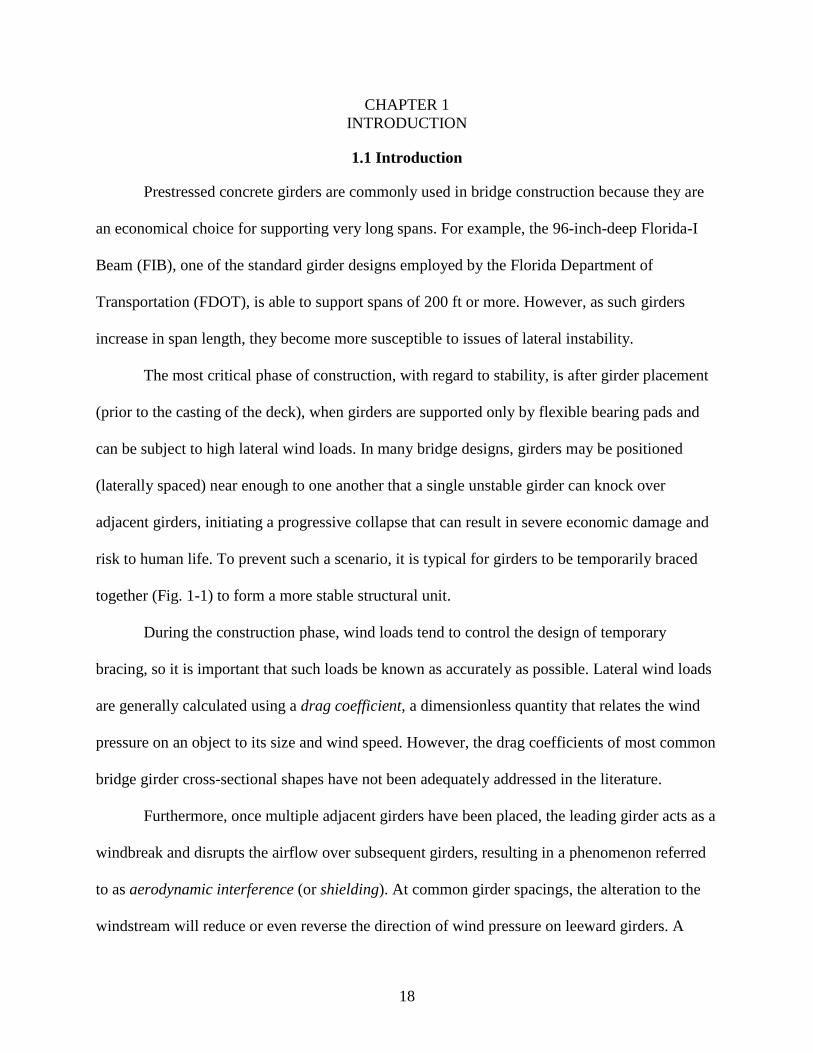
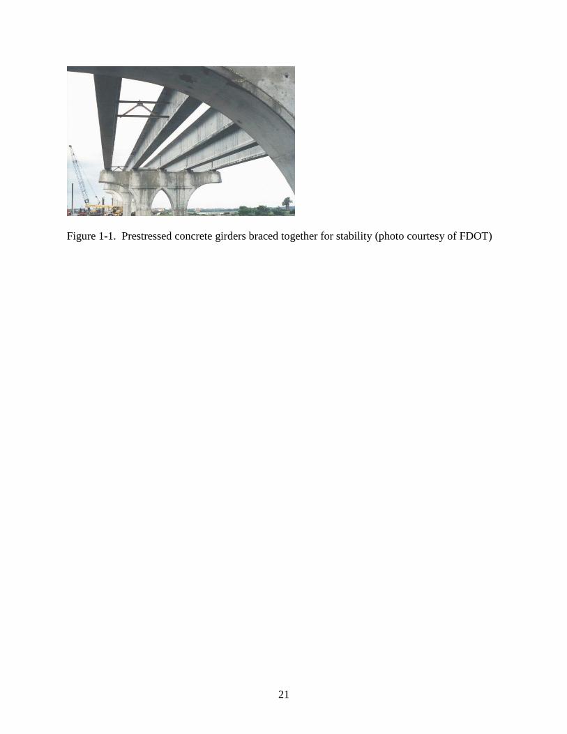
together (Fig. 1-1) to form a more stable structural unit.
During the construction phase, wind loads tend to control the design of temporary
bracing, so it is important that such loads be known as accurately as possible. Lateral wind loads
are generally calculated using a drag coefficient, a dimensionless quantity that relates the wind
pressure on an object to its size and wind speed. However, the drag coefficients of most common
bridge girder cross-sectional shapes have not been adequately addressed in the literature.
Furthermore, once multiple adjacent girders have been placed, the leading girder acts as a
windbreak and disrupts the airflow over subsequent girders, resulting in a phenomenon referred
to as aerodynamic interference (or shielding). At common girder spacings, the alteration to the
windstream will reduce or even reverse the direction of wind pressure on leeward girders. A

19
thorough understanding of this shielding effect is necessary to develop appropriately
conservative bracing design forces. However, this area has also received little attention in the
literature.
1.2 Objectives
The primary objective of this research was to experimentally quantify drag coefficients
for common bridge girder shapes as well as shielding effects arising from the aerodynamic
interference between adjacent girders, and to synthesize the results into a set of conservative
design parameters that can be used to compute lateral wind loads for design and construction
calculations. A secondary objective was to use analytical models of braced girder systems to
develop recommendations for temporary bracing of prestressed concrete girders (FIBs) subjected
to the new design wind loads.
1.3 Scope of Work
Experimental testing: Wind tunnel tests were performed to measure the aerodynamic
coefficients (drag, lift, and torque) of five (5) bridge girder cross-sectional shapes [two
(2) plate girder; two (2) FIB; and one open-top box], chosen to be representative of a
wide range modern Florida bridges. In addition to measuring the aerodynamic
coefficients of the individual girders, tests were performed on groups of adjacent girders
in a variety of common configurations in order to quantify the shielding effects caused by
aerodynamic interference.
Design wind loads: Measurements from the wind tunnel tests were analyzed to identify
common trends and to develop a conservative set of simplified wind load parameters that
are suitable for use in design.
Analysis method for bearing pad stiffnesses: Experimental bearing pad stiffness
measurements from a previous FDOT research project (BDK75 977-03, Consolazio et al.
2012) were used to develop and validate a new analytical method for estimating the
girder support stiffnesses provided by steel-reinforced elastomeric bearing pads.
System-level analytical models: Analytical models were developed that were capable of
evaluating the lateral stability of Florida-I Beams (FIBs). The models incorporated the
estimated support stiffnesses provided by standard FDOT bearing pads and were capable
of capturing system-level behavior of multiple girders braced together with any of several
common brace types.

20
Wind load capacity of individual FIBs: An analytical parametric study was conducted
to determine a simplified equation for estimating the maximum wind pressure that an
individual (unbraced) FIB can resist without becoming unstable.
Recommendations for temporary bracing: Analytical parametric studies were
conducted using the system-level models and the design wind loads to evaluate
temporary bracing requirements for FIB systems in a variety of configurations. In
addition to general recommendations for temporary bracing design, the results of the
parametric study were used to develop simplified equations for estimating the capacity of
braced systems of FIBs.
21
Figure 1-1. Prestressed concrete girders braced together for stability (photo courtesy of FDOT)
22
CHAPTER 2
PHYSICAL DESCRIPTION OF BRIDGES DURING CONSTRUCTION
2.1 Introduction
This study is concerned with the stability of long-span prestressed concrete girders during
the construction process. Specifically, the girders under investigation are Florida-I Beams (FIBs),
a family of standard cross-sectional shapes of varying depths that are commonly employed in
bridge designs in Florida. These beams are typically cast offsite, transported to the construction
site by truck, then lifted into position one-at-a-time by crane, where they are placed on
elastomeric bearing pads and braced together for stability. It is this stage of construction, prior to
the casting of the deck that is primarily of interest. In this chapter, a physical description of the
construction-stage bridge structures under consideration in this study will be provided along with
the definition of relevant terminology.
2.2 Geometric Parameters
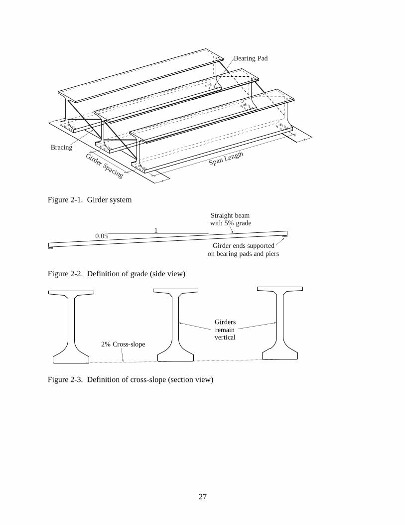
The term girder system will be used to refer to a group of one or more FIBs braced
together in an evenly spaced row (Figure 2-1). In addition to span length and spacing, there are
several geometric parameters that define the shape and placement of the girders within a system.
They are:
Grade: Longitudinal incline of the girders, typically expressed as a percentage of rise per
unit of horizontal length (Figure 2-2).
Cross-slope: The transverse incline (slope) of the deck, expressed as a percentage, which
results in girders that are staggered vertically (Figure 2-3).
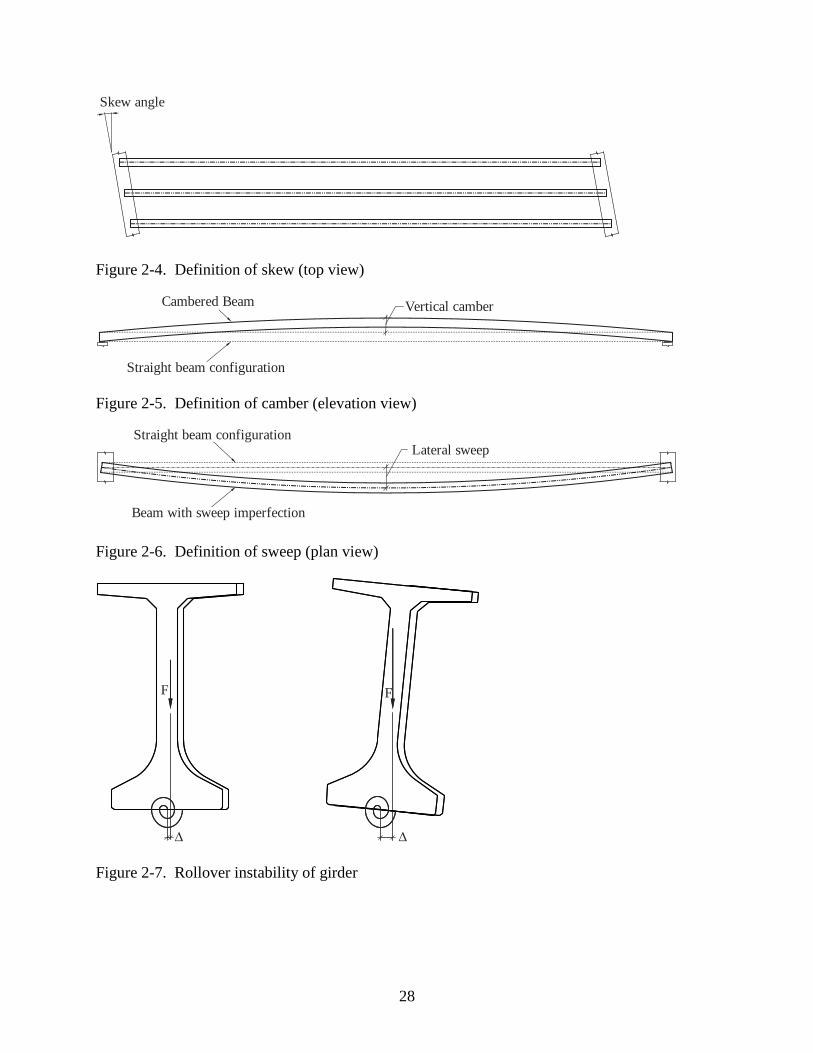
Skew angle: Longitudinal staggering of girders, due to pier caps that are not
perpendicular to the girder axes (Figure 2-4).
Camber: Vertical bowing of the girder (Figure 2-5) due to prestressing in the bottom
flange expressed as the maximum vertical deviation from a perfectly straight line
connecting one end of the girder to the other. Note that the total amount of vertical
camber immediately following girder placement is larger than the camber in the
completed bridge structure because the weight of the deck is not yet present.
23
Sweep: Lateral bowing of the girder (Figure 2-6) due to manufacturing imperfections,
expressed as the maximum horizontal deviation from a perfectly straight line connecting
one end of the girder to the other.
2.3 Bearing Pads
Bridge girders rest directly on steel-reinforced neoprene bearing pads which are the only
points of contact between the girder and the substructure. There is generally sufficient friction
between the pad and other structural components so that any movement of a girder relative to the
substructure (with the exception of vertical uplift) must also move the top surface of the pad
relative to the bottom surface. As a result, the girder support conditions in all six degrees of
freedom can be represented as finite stiffnesses that correspond to the equivalent deformation
modes of the pad. These deformation modes fall into four categories: shear, compression (axial),
rotation (e.g., roll), and torsion. Calculation of these stiffnesses is addressed in Chapter 6.
2.4 Sources of Lateral Instability
Girder instability arises when the structural deformations caused by application of a load
act to increase the moment arm of that load to such an extent that equilibrium cannot be
achieved. The additional moment (often called the secondary effects) causes the structure to
deform further, which increases the moment arm even more. In a stable system, this process
continues until the structure converges on a deformed state in which static equilibrium is
achieved. However, if the load exceeds some critical value (i.e., the buckling load), the system
becomes unstable, in which case the process diverges and the structural deformations increase
without bound (i.e., the structure collapses). Long-span bridge girders are susceptible to two
primary modes of instability: girder rollover and lateral-torsional buckling.
Girder rollover refers to the rigid-body rotation of a girder with sweep imperfections
resting on end supports (i.e., bearing pads) that have a finite roll stiffness. Sweep imperfections
cause the force resultant of the girder self-weight (F) to be offset a small distance (Δ) from the
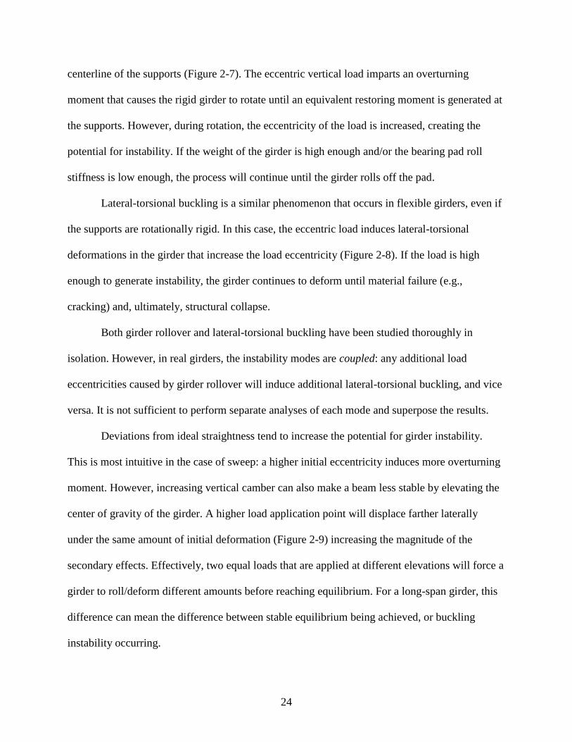
24
centerline of the supports (Figure 2-7). The eccentric vertical load imparts an overturning
moment that causes the rigid girder to rotate until an equivalent restoring moment is generated at
the supports. However, during rotation, the eccentricity of the load is increased, creating the
potential for instability. If the weight of the girder is high enough and/or the bearing pad roll
stiffness is low enough, the process will continue until the girder rolls off the pad.
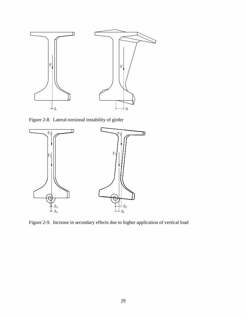
Lateral-torsional buckling is a similar phenomenon that occurs in flexible girders, even if
the supports are rotationally rigid. In this case, the eccentric load induces lateral-torsional
deformations in the girder that increase the load eccentricity (Figure 2-8). If the load is high
enough to generate instability, the girder continues to deform until material failure (e.g.,
cracking) and, ultimately, structural collapse.
Both girder rollover and lateral-torsional buckling have been studied thoroughly in
isolation. However, in real girders, the instability modes are coupled: any additional load
eccentricities caused by girder rollover will induce additional lateral-torsional buckling, and vice
versa. It is not sufficient to perform separate analyses of each mode and superpose the results.
Deviations from ideal straightness tend to increase the potential for girder instability.
This is most intuitive in the case of sweep: a higher initial eccentricity induces more overturning
moment. However, increasing vertical camber can also make a beam less stable by elevating the
center of gravity of the girder. A higher load application point will displace farther laterally
under the same amount of initial deformation (Figure 2-9) increasing the magnitude of the
secondary effects. Effectively, two equal loads that are applied at different elevations will force a
girder to roll/deform different amounts before reaching equilibrium. For a long-span girder, this
difference can mean the difference between stable equilibrium being achieved, or buckling
instability occurring.

25
2.5 Lateral Wind Loads
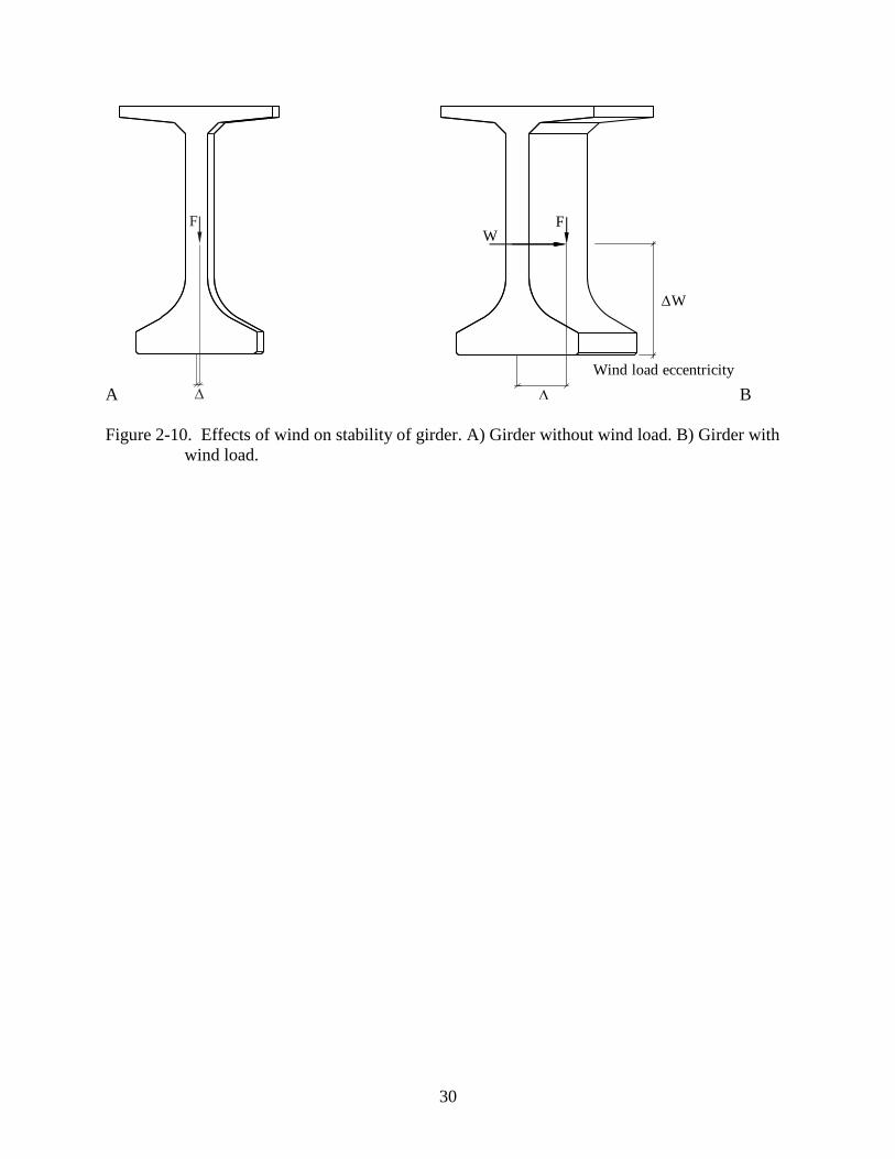
In addition to gravity induced self-weight, girder systems are also subjected to
intermittent lateral wind loads of varying intensity throughout the construction process. Wind
loads are generally modeled as uniform pressure loads applied to girders in the lateral
(transverse) direction. These types of loads can have a severely destabilizing effect on girder
systems. Because the force resultant at the center of pressure (W) is offset from the bearing pad
supports, large overturning moments can be generated that contribute directly to girder rollover.
Furthermore, the wind force causes the girders to bend laterally (about their weak axes). This can
increase the eccentricity of the self-weight, increasing the potential for instability (Figure 2-10).
2.6 Temporary Bracing
During construction, girders are often braced to prevent lateral instability from arising.
Usually, these braces are temporary and are removed after the deck is cast. Bracing is divided
into two basic types: anchor bracing and girder-to-girder bracing.
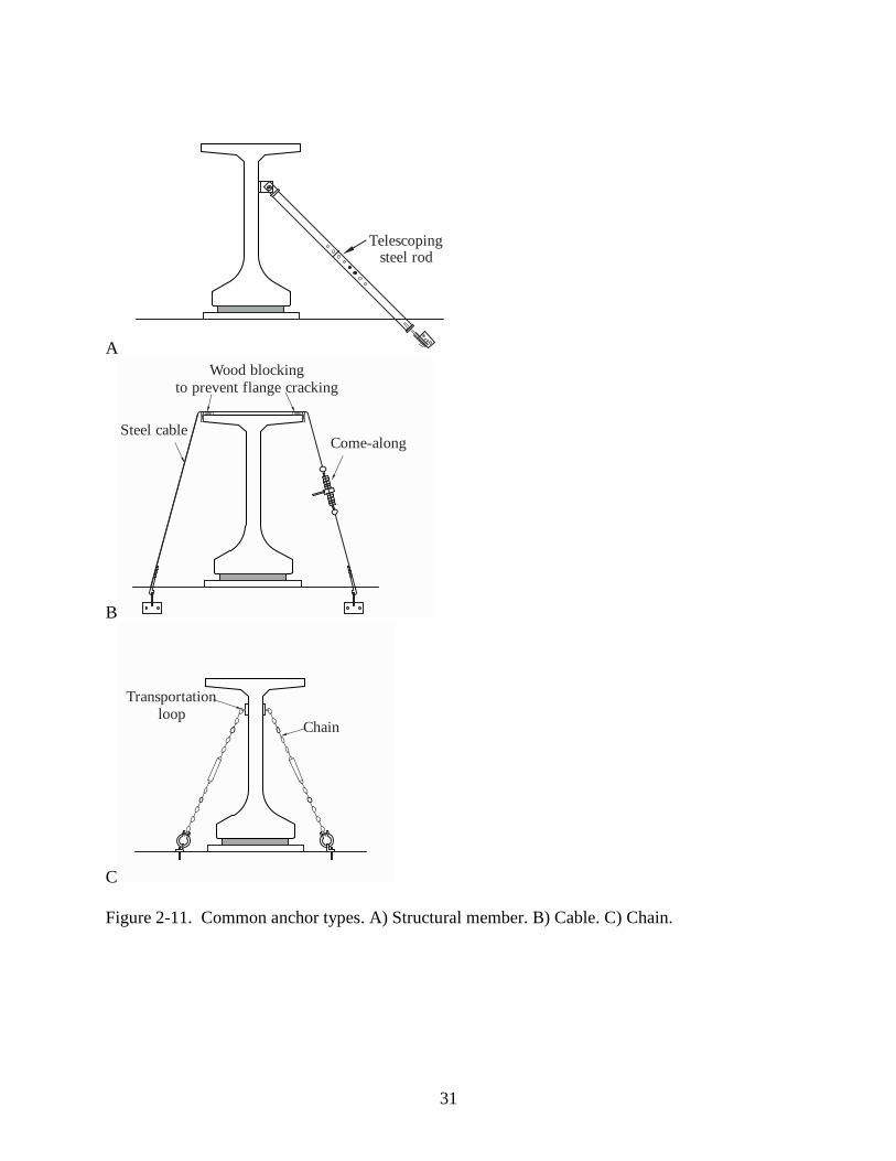
2.6.1 Anchor Bracing
Because the first girder in the erection sequence has no adjacent girders to brace against,
anchors are used to brace the ends of the girder to the pier. Anchors can take the form of inclined
structural members such as telescoping steel rods (Figure 2-11a) or tension-only members such
as cables (Figure 2-11b) or chains (Figure 2-11c). In addition to their lateral incline, it is
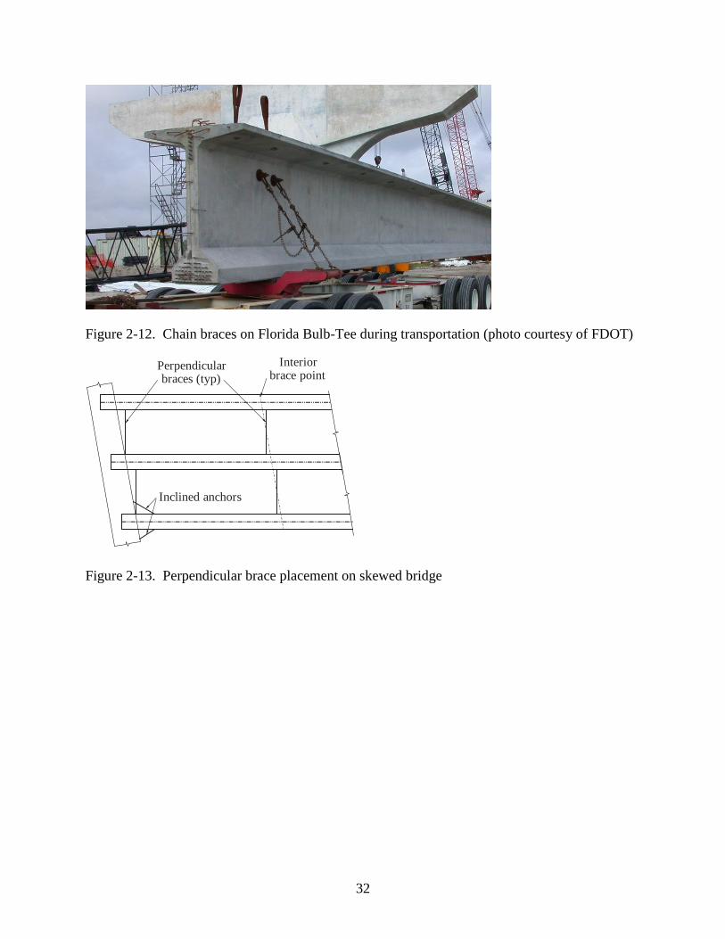
common for anchors to also be inclined inward (towards the center of the span) so that they can
reuse the same precast connections that are used to stabilize girders during transportation
(Figure 2-12).
Anchors are generally not as effective as girder-to-girder bracing; because they can only
restrain the girders at the ends, they can prevent girder rollover but not lateral-torsional buckling.
26
For this reason, anchors are generally only used on the first girder to be erected and are not used
on subsequent girders.
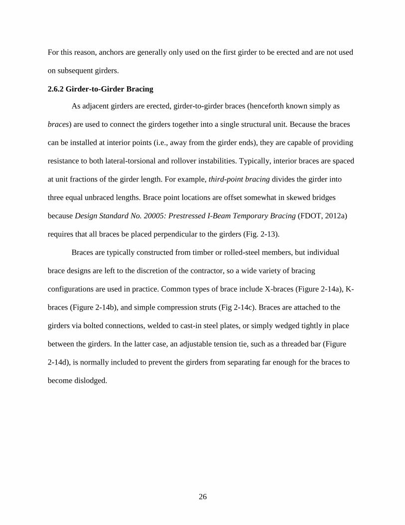
2.6.2 Girder-to-Girder Bracing
As adjacent girders are erected, girder-to-girder braces (henceforth known simply as
braces) are used to connect the girders together into a single structural unit. Because the braces
can be installed at interior points (i.e., away from the girder ends), they are capable of providing
resistance to both lateral-torsional and rollover instabilities. Typically, interior braces are spaced
at unit fractions of the girder length. For example, third-point bracing divides the girder into
three equal unbraced lengths. Brace point locations are offset somewhat in skewed bridges
because Design Standard No. 20005: Prestressed I-Beam Temporary Bracing (FDOT, 2012a)
requires that all braces be placed perpendicular to the girders (Fig. 2-13).
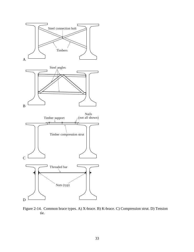
Braces are typically constructed from timber or rolled-steel members, but individual
brace designs are left to the discretion of the contractor, so a wide variety of bracing
configurations are used in practice. Common types of brace include X-braces (Figure 2-14a), K-
braces (Figure 2-14b), and simple compression struts (Fig 2-14c). Braces are attached to the
girders via bolted connections, welded to cast-in steel plates, or simply wedged tightly in place
between the girders. In the latter case, an adjustable tension tie, such as a threaded bar (Figure
2-14d), is normally included to prevent the girders from separating far enough for the braces to
become dislodged.
27
Span LengthGirder Spacing
Bracing
Bearing Pad
Figure 2-1. Girder system
Straight beamwith 5% grade
10.05
Girder ends supported
on bearing pads and piers
Figure 2-2. Definition of grade (side view)
Girders
remain vertical
2% Cross-slope
Figure 2-3. Definition of cross-slope (section view)
28
Skew angle
Figure 2-4. Definition of skew (top view)
Cambered Beam
Straight beam configuration
Vertical camber
Figure 2-5. Definition of camber (elevation view)
Beam with sweep imperfection
Straight beam configurationLateral sweep
Figure 2-6. Definition of sweep (plan view)
F
F
Figure 2-7. Rollover instability of girder
29
F F
Figure 2-8. Lateral-torsional instability of girder
F1
F2
F2
F1
Figure 2-9. Increase in secondary effects due to higher application of vertical load
30
A
F
W
WF
Wind load eccentricity
B
Figure 2-10. Effects of wind on stability of girder. A) Girder without wind load. B) Girder with
wind load.
31
A
Telescopingsteel rod
B
Steel cable
Wood blocking
to prevent flange cracking
Come-along
C
Chain
Transportation
loop
Figure 2-11. Common anchor types. A) Structural member. B) Cable. C) Chain.
32
Figure 2-12. Chain braces on Florida Bulb-Tee during transportation (photo courtesy of FDOT)
Inclined anchors
Interiorbrace point
Perpendicularbraces (typ)
Figure 2-13. Perpendicular brace placement on skewed bridge
33
A
Timbers
Steel connection bolt
B
Steel angles
C
Timber compression strut
Timber support
Nails (not all shown)
D
Threaded bar
Nuts (typ)
Figure 2-14. Common brace types. A) X-brace. B) K-brace. C) Compression strut. D) Tension
tie.
34
CHAPTER 3
BACKGROUND ON DRAG COEFFICIENTS
3.1 Introduction
In order to calculate the wind load on a bridge girder, it is necessary to know the drag
coefficient for the girder cross-sectional shape. The drag coefficient is a type of aerodynamic
coefficient: a dimensionless factor that relates the magnitude of the fluid force on a particular
geometric shape to the approaching wind speed. Drag coefficients are typically a function of the
relative orientation of the object with the direction of the impinging wind.
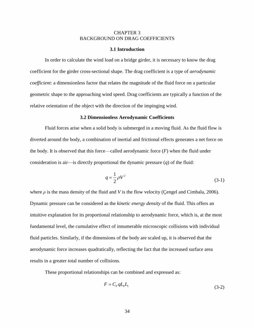
3.2 Dimensionless Aerodynamic Coefficients
Fluid forces arise when a solid body is submerged in a moving fluid. As the fluid flow is
diverted around the body, a combination of inertial and frictional effects generates a net force on
the body. It is observed that this force—called aerodynamic force (F) when the fluid under
consideration is air—is directly proportional the dynamic pressure (q) of the fluid:
21
2q V
(3-1)
where ρ is the mass density of the fluid and V is the flow velocity (Çengel and Cimbala, 2006).
Dynamic pressure can be considered as the kinetic energy density of the fluid. This offers an
intuitive explanation for its proportional relationship to aerodynamic force, which is, at the most
fundamental level, the cumulative effect of innumerable microscopic collisions with individual
fluid particles. Similarly, if the dimensions of the body are scaled up, it is observed that the
aerodynamic force increases quadratically, reflecting the fact that the increased surface area
results in a greater total number of collisions.
These proportional relationships can be combined and expressed as:
0 1FF C qL L (3-2)

35
where L0 and L1 are arbitrary reference lengths and CF is a combined proportionality factor,
called a force coefficient. The selection of L0 and L1 does not affect the validity of Equation 3-2
as long as they both scale with the structure. However, it is important to be consistent; force
coefficients that use different reference lengths are not directly comparable, and a coefficient for
which the reference lengths are not explicitly known is useless for predicting aerodynamic
forces. In structural applications, it is common for the product L0L1 to be expressed in the form
of a reference area, A, which is typically taken as the projected area of the structure in the
direction of wind.
By an analogous process, it is possible to derive a moment coefficient (CM), which
normalizes aerodynamic moment load in the same way that the force coefficient normalizes
aerodynamic force. The only difference is that aerodynamic moment grows cubically with body
size rather than quadratically (because the moment arms of the individual collisions grow along
with the surface area). Therefore, the moment proportionality expression is:
0 1 2MM C qL L L (3-3)
As with the force coefficient, the reference lengths must be known in order to properly interpret
the CM. However, with moment coefficients, it is equally important to know the center of
rotation about which the normalized moment acts. Together, CF and CM are called aerodynamic
coefficients, and they can be used to fully describe the three-dimensional state of aerodynamic
load on a structure (for a particular wind direction).
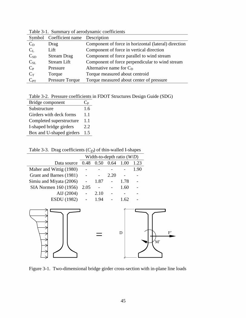
When working with bridge girders, or other straight, slender members, it is often
convenient to assume that the length of the girder is effectively infinite. This simplifies
engineering calculations by reducing the girder to a two-dimensional cross-section subjected to
in-plane aerodynamic line-loads (Figure 3-1). Depending on the direction of wind, out-of-plane

36
forces and moments may exist, but they generally do not contribute to the load cases that control
design and can therefore be considered negligible. In two dimensions, the proportionality
expressions for the aerodynamic coefficients become:
1FF C qL (3-4)
1 2MM C qL L (3-5)
where F′ is a distributed force (force per unit length) and M′ is a distributed torque (moment per
unit length). Note that two-dimensional aerodynamic coefficients can be used interchangeably in
the three-dimensional formulation if one reference length (L0) is taken to be the out-of-plane
length of the girder. All further discussions of aerodynamic coefficients in this report will use the
two-dimensional formulation unless stated otherwise. The remaining reference lengths (L1 and
L2) will always be taken as the girder depth, D, so that the force and moment coefficients are
defined as:
21
2
F
FC
V D
(3-6)
2 21
2
M
MC
V D
(3-7)
Aerodynamic coefficients are sometimes called shape factors because they represent the
contribution of the geometry of an object (i.e., the way airflow is diverted around it),
independent of the scale of the object or the intensity of the flow. Because of the complexity of
the differential equations governing fluid flow, the aerodynamic coefficients of a structure are
not calculated from first principles but can, instead, be measured directly in a wind tunnel using
reduced-scale models.

37
3.3 Terminology Related to Aerodynamic Coefficients
Aerodynamic force on a body is typically resolved into two orthogonal components, drag
and lift. These components have corresponding force coefficients: the drag coefficient (CD) and
lift coefficient (CL). In this report, drag is defined as the lateral component of force and lift is
defined as the vertical component of force, regardless of the angle of the applied wind.
In several subfields of fluid dynamics, it is more conventional to define drag as the
component of force along the direction of the wind stream and lift as the component
perpendicular to the wind stream. However, this is inconvenient when evaluating wind loads on
stationary structures (e.g., bridge girders) because the angle of the wind stream can change over
time. Where necessary in this report, the names stream drag (CSD) and stream lift (CSL) (Figure
3-2) will be used to refer to the force components that are aligned with, and perpendicular to, the
wind stream.
Finally, the term pressure coefficient (CP), is an alternative name for CD, and is often
used in design codes to indicate that it is to be used to calculate a wind pressure load (P) rather
than a total force, as in:
21
2PP C V
(3-8)
This is advantageous because it obviates the need to explicitly specify the characteristic
dimensions that were used to normalize the coefficient. Instead, denormalization occurs
implicitly when the pressure load is applied over the projected surface area of the structure.
Unfortunately, this approach breaks down when working with drag and lift coefficients together.
If drag and lift are both represented as pressure loads, then the areas used to normalize the
coefficients will differ (unless by chance the depth and width of the structure are equal). As a
result, the magnitudes of the coefficients are not directly comparable—that is, equal coefficients
38
will not produce loads of equal magnitude—and they cannot be treated mathematically as
components of a single force vector, which complicates coordinate transformations and other
operations. For this reason, the term pressure coefficient is not used in this report, except when in
reference to design codes that use the term.
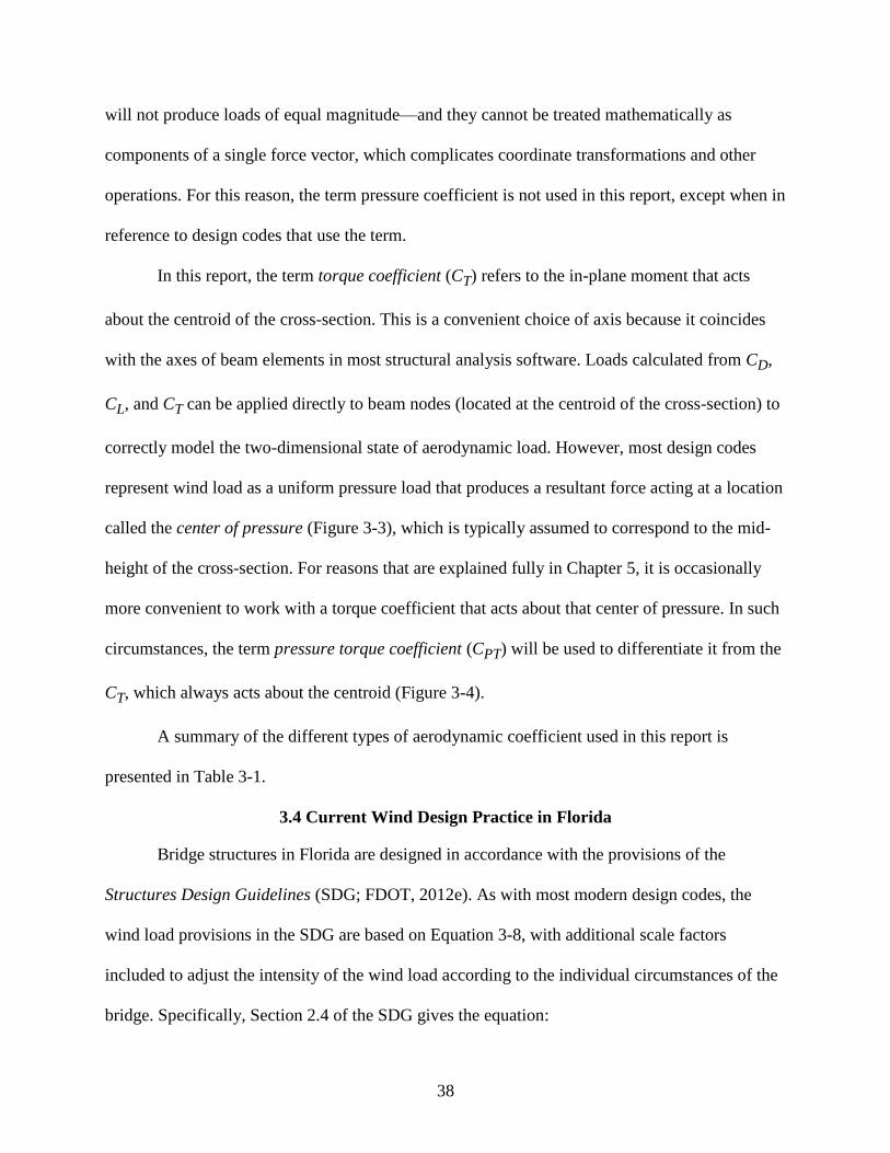
In this report, the term torque coefficient (CT) refers to the in-plane moment that acts
about the centroid of the cross-section. This is a convenient choice of axis because it coincides
with the axes of beam elements in most structural analysis software. Loads calculated from CD,
CL, and CT can be applied directly to beam nodes (located at the centroid of the cross-section) to
correctly model the two-dimensional state of aerodynamic load. However, most design codes
represent wind load as a uniform pressure load that produces a resultant force acting at a location
called the center of pressure (Figure 3-3), which is typically assumed to correspond to the mid-
height of the cross-section. For reasons that are explained fully in Chapter 5, it is occasionally
more convenient to work with a torque coefficient that acts about that center of pressure. In such
circumstances, the term pressure torque coefficient (CPT) will be used to differentiate it from the
CT, which always acts about the centroid (Figure 3-4).
A summary of the different types of aerodynamic coefficient used in this report is
presented in Table 3-1.
3.4 Current Wind Design Practice in Florida
Bridge structures in Florida are designed in accordance with the provisions of the
Structures Design Guidelines (SDG; FDOT, 2012e). As with most modern design codes, the
wind load provisions in the SDG are based on Equation 3-8, with additional scale factors
included to adjust the intensity of the wind load according to the individual circumstances of the
bridge. Specifically, Section 2.4 of the SDG gives the equation:
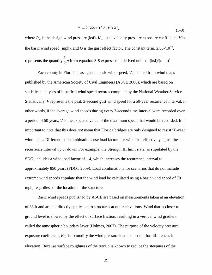
39
6 22.56 10Z Z PP K V GC (3-9)
where PZ is the design wind pressure (ksf), KZ is the velocity pressure exposure coefficient, V is
the basic wind speed (mph), and G is the gust effect factor. The constant term, 2.56×10⁻⁶
,
represents the quantity 1
2 ρ from equation 3-8 expressed in derived units of (ksf)/(mph)
2.
Each county in Florida is assigned a basic wind speed, V, adapted from wind maps
published by the American Society of Civil Engineers (ASCE 2006), which are based on
statistical analyses of historical wind speed records compiled by the National Weather Service.
Statistically, V represents the peak 3-second gust wind speed for a 50-year recurrence interval. In
other words, if the average wind speeds during every 3-second time interval were recorded over
a period of 50 years, V is the expected value of the maximum speed that would be recorded. It is
important to note that this does not mean that Florida bridges are only designed to resist 50-year
wind loads. Different load combinations use load factors for wind that effectively adjust the
recurrence interval up or down. For example, the Strength III limit state, as stipulated by the
SDG, includes a wind load factor of 1.4, which increases the recurrence interval to
approximately 850 years (FDOT 2009). Load combinations for scenarios that do not include
extreme wind speeds stipulate that the wind load be calculated using a basic wind speed of 70
mph, regardless of the location of the structure.
Basic wind speeds published by ASCE are based on measurements taken at an elevation
of 33 ft and are not directly applicable to structures at other elevations. Wind that is closer to
ground level is slowed by the effect of surface friction, resulting in a vertical wind gradient
called the atmospheric boundary layer (Holmes, 2007). The purpose of the velocity pressure
exposure coefficient, KZ, is to modify the wind pressure load to account for differences in
elevation. Because surface roughness of the terrain is known to reduce the steepness of the
40
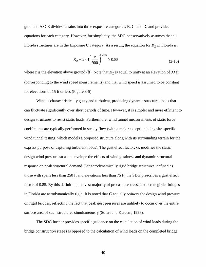
gradient, ASCE divides terrains into three exposure categories, B, C, and D, and provides
equations for each category. However, for simplicity, the SDG conservatively assumes that all
Florida structures are in the Exposure C category. As a result, the equation for KZ in Florida is:
0.2105
2.01 0.85900
Z
zK
(3-10)
where z is the elevation above ground (ft). Note that KZ is equal to unity at an elevation of 33 ft
(corresponding to the wind speed measurements) and that wind speed is assumed to be constant
for elevations of 15 ft or less (Figure 3-5).
Wind is characteristically gusty and turbulent, producing dynamic structural loads that
can fluctuate significantly over short periods of time. However, it is simpler and more efficient to
design structures to resist static loads. Furthermore, wind tunnel measurements of static force
coefficients are typically performed in steady flow (with a major exception being site-specific
wind tunnel testing, which models a proposed structure along with its surrounding terrain for the
express purpose of capturing turbulent loads). The gust effect factor, G, modifies the static
design wind pressure so as to envelope the effects of wind gustiness and dynamic structural
response on peak structural demand. For aerodynamically rigid bridge structures, defined as
those with spans less than 250 ft and elevations less than 75 ft, the SDG prescribes a gust effect
factor of 0.85. By this definition, the vast majority of precast prestressed concrete girder bridges
in Florida are aerodynamically rigid. It is noted that G actually reduces the design wind pressure
on rigid bridges, reflecting the fact that peak gust pressures are unlikely to occur over the entire
surface area of such structures simultaneously (Solari and Kareem, 1998).
The SDG further provides specific guidance on the calculation of wind loads during the
bridge construction stage (as opposed to the calculation of wind loads on the completed bridge
41
structure). If the exposure period of the construction stage is less than one year, a reduction
factor of 0.6 on the basic wind speed is allowed by the SDG. During active construction, the
basic wind speed can be further reduced to a base level of 20 mph. Temporary bracing must be
designed for three load cases: Girder Placement (construction active), Braced Girder
(construction inactive), and Deck Placement (construction active).
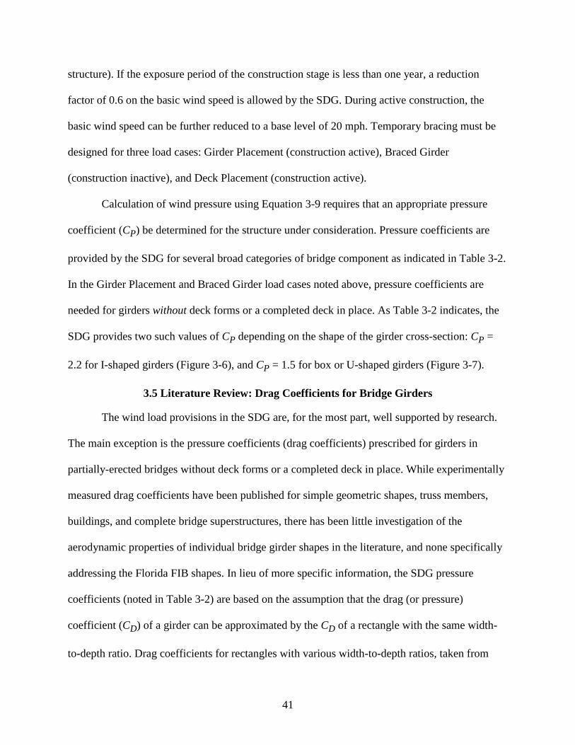
Calculation of wind pressure using Equation 3-9 requires that an appropriate pressure
coefficient (CP) be determined for the structure under consideration. Pressure coefficients are
provided by the SDG for several broad categories of bridge component as indicated in Table 3-2.
In the Girder Placement and Braced Girder load cases noted above, pressure coefficients are
needed for girders without deck forms or a completed deck in place. As Table 3-2 indicates, the
SDG provides two such values of CP depending on the shape of the girder cross-section: CP =
2.2 for I-shaped girders (Figure 3-6), and CP = 1.5 for box or U-shaped girders (Figure 3-7).
3.5 Literature Review: Drag Coefficients for Bridge Girders
The wind load provisions in the SDG are, for the most part, well supported by research.
The main exception is the pressure coefficients (drag coefficients) prescribed for girders in
partially-erected bridges without deck forms or a completed deck in place. While experimentally
measured drag coefficients have been published for simple geometric shapes, truss members,
buildings, and complete bridge superstructures, there has been little investigation of the
aerodynamic properties of individual bridge girder shapes in the literature, and none specifically
addressing the Florida FIB shapes. In lieu of more specific information, the SDG pressure
coefficients (noted in Table 3-2) are based on the assumption that the drag (or pressure)
coefficient (CD) of a girder can be approximated by the CD of a rectangle with the same width-
to-depth ratio. Drag coefficients for rectangles with various width-to-depth ratios, taken from
42
Holmes (2007) and other sources, are shown in Figure 3-8. It is clear that there is significant
variation of CD as the width-to-depth (W/D) ratio changes. Also shown in the figure are W/D
ranges for typical girder types common to the state of Florida. Finally, W/D values for the
specific girder cross-sectional shapes tested (in a wind tunnel) in this study are also indicated
(additional details regarding these shapes will be provided in Chapter 4).
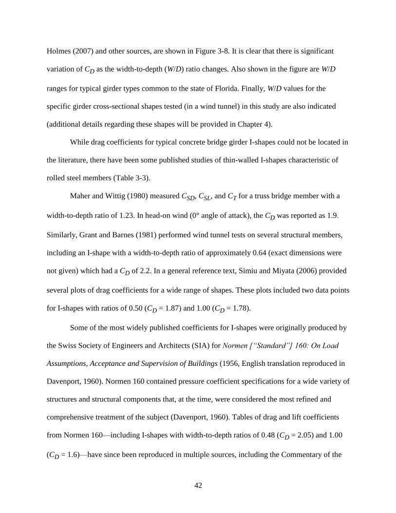
While drag coefficients for typical concrete bridge girder I-shapes could not be located in
the literature, there have been some published studies of thin-walled I-shapes characteristic of
rolled steel members (Table 3-3).
Maher and Wittig (1980) measured CSD, CSL, and CT for a truss bridge member with a
width-to-depth ratio of 1.23. In head-on wind (0° angle of attack), the CD was reported as 1.9.
Similarly, Grant and Barnes (1981) performed wind tunnel tests on several structural members,
including an I-shape with a width-to-depth ratio of approximately 0.64 (exact dimensions were
not given) which had a CD of 2.2. In a general reference text, Simiu and Miyata (2006) provided
several plots of drag coefficients for a wide range of shapes. These plots included two data points
for I-shapes with ratios of 0.50 (CD = 1.87) and 1.00 (CD = 1.78).
Some of the most widely published coefficients for I-shapes were originally produced by
the Swiss Society of Engineers and Architects (SIA) for Normen [“Standard”] 160: On Load
Assumptions, Acceptance and Supervision of Buildings (1956, English translation reproduced in
Davenport, 1960). Normen 160 contained pressure coefficient specifications for a wide variety of
structures and structural components that, at the time, were considered the most refined and
comprehensive treatment of the subject (Davenport, 1960). Tables of drag and lift coefficients
from Normen 160—including I-shapes with width-to-depth ratios of 0.48 (CD = 2.05) and 1.00
(CD = 1.6)—have since been reproduced in multiple sources, including the Commentary of the

43
National Building Code (NBC) of Canada (NRC, 2005; Sachs, 1978; Scruton and Newberry,
1963). The exact origins of the coefficients are unknown, but the NBC commentary states that
they were based on “wind-tunnel experiments”.
Other jurisdictions provide varying levels of guidance regarding drag coefficients for I-
shapes. In Japan, the de facto design code (AIJ, 2004) includes a CD of 2.1 for an I-shape with a
width-to-depth ratio of 0.50. The AIJ commentary cites an unobtainable Japanese-language
paper as the source of this value. Great Britain, like the FDOT, assumes that the girder cross-
sections are aerodynamically similar to rectangles, and provides a plot (reproduced in Figure 3-8)
for selecting the coefficient based on the width-to-depth ratio of the cross-section (BSI, 2006).
The European Union simply recommends a blanket value of 2.0 for all “sharp-edged structural
sections” (CEN 2004).
ESDU, a non-governmental organization that produces engineering reference materials,
has performed its own literature review of drag coefficients for structural members, and it has
published a reference (ESDU, 1982) that synthesizes data from multiple sources, including
several of those discussed above and several foreign language sources. Drag coefficients are
provided for I-shapes with width-to-depth ratios of 0.50 (CD = 1.94) and 1.00 (CD = 1.62), with
an estimated uncertainty of approximately ±15%. Interpolation between the two data points is
encouraged.
All of the I-shapes investigated in the literature are for basic truss or building members
and did not include any width-to-depth ratios less than approximately 1/2. However, most steel I-
shapes used in long-span bridge girders have width-to-depth ratios that range roughly from 1/6 to
1/3. Because CD tends to vary with width-to-depth ratio, there is no reason to believe that the
results of these studies are directly applicable to steel bridge girders. Furthermore, when the data

44
are plotted (Figure 3-9), it becomes clear that the equivalent rectangle is a poor (albeit
conservative) predictor of aerodynamic properties.
Regarding box girders, the SDG provides a value of 1.5, which is a common choice for
box-shaped bridge decks. However, before the deck is cast, the top of the girder is open. A
search of the literature found only one source that discusses the aerodynamic properties of open-
top box girders. Myers and Ghalib (n.d.) used a two-dimensional computational fluid dynamics
analysis to calculate the drag on a pair of such girders. While coefficients for the individual
girders were not provided, they concluded that drag coefficients can be significantly higher on a
girder with an open top.
45
Table 3-1. Summary of aerodynamic coefficients
Symbol Coefficient name Description
CD Drag Component of force in horizontal (lateral) direction
CL Lift Component of force in vertical direction
CSD Stream Drag Component of force parallel to wind stream
CSL Stream Lift Component of force perpendicular to wind stream
CP Pressure Alternative name for CD
CT Torque Torque measured about centroid
CPT Pressure Torque Torque measured about center of pressure
Table 3-2. Pressure coefficients in FDOT Structures Design Guide (SDG)
Bridge component CP
Substructure 1.6
Girders with deck forms 1.1
Completed superstructure 1.1
I-shaped bridge girders 2.2
Box and U-shaped girders 1.5
Table 3-3. Drag coefficients (CD) of thin-walled I-shapes
Width-to-depth ratio (W/D)
Data source 0.48 0.50 0.64 1.00 1.23
Maher and Wittig (1980) - - - - 1.90
Grant and Barnes (1981) - - 2.20 - -
Simiu and Miyata (2006) - 1.87 - 1.78 -
SIA Normen 160 (1956) 2.05 - - 1.60 -
AIJ (2004) - 2.10 - - -
ESDU (1982) - 1.94 - 1.62 -
M′
F′D=
Figure 3-1. Two-dimensional bridge girder cross-section with in-plane line loads
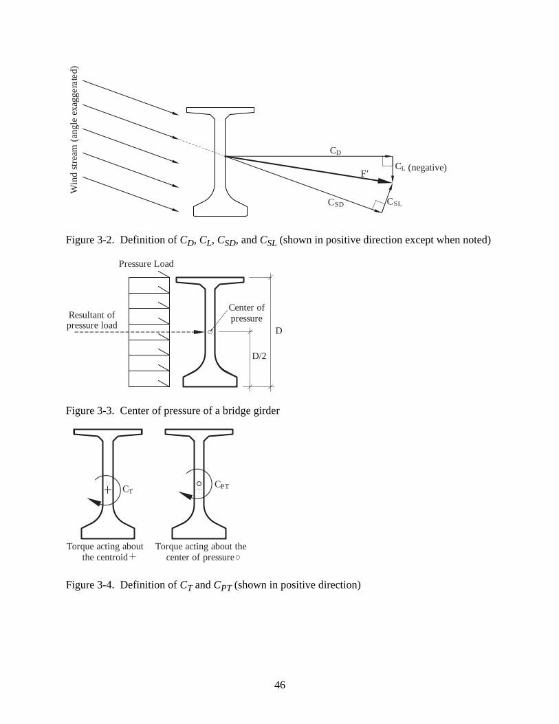
46
Win
d s
trea
m (
angle
exag
ge
rate
d)
CD
CSD
CL
CSL
(negative)F′
Figure 3-2. Definition of CD, CL, CSD, and CSL (shown in positive direction except when noted)
Pressure Load
Resultant of pressure load
Center of
pressure
D
D/2
Figure 3-3. Center of pressure of a bridge girder
CTCPT
Torque acting about the
center of pressure
Torque acting about
the centroid
Figure 3-4. Definition of CT and CPT (shown in positive direction)
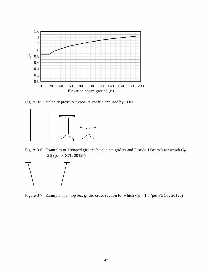
47
Figure 3-5. Velocity pressure exposure coefficient used by FDOT
Figure 3-6. Examples of I-shaped girders (steel plate girders and Florida-I Beams) for which CP
= 2.2 (per FDOT, 2012e)
Figure 3-7. Example open top box girder cross-section for which CP = 1.5 (per FDOT, 2012e)
Elevation above ground (ft)
KZ
0 20 40 60 80 100 120 140 160 180 200
0.0
0.2
0.4
0.6
0.8
1.0
1.2
1.4
1.6
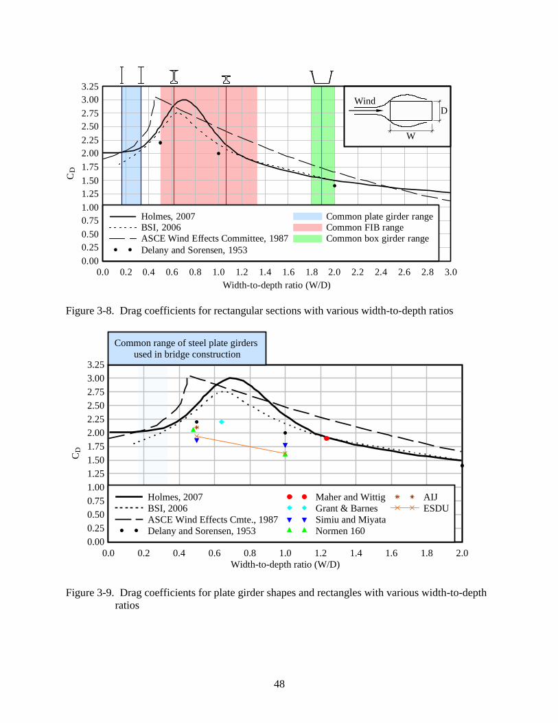
48
Width-to-depth ratio (W/D)
CD
0.0 0.2 0.4 0.6 0.8 1.0 1.2 1.4 1.6 1.8 2.0 2.2 2.4 2.6 2.8 3.0
0.00
0.25
0.50
0.75
1.00
1.25
1.50
1.75
2.00
2.25
2.50
2.75
3.00
3.25
Holmes, 2007
BSI, 2006
ASCE Wind Effects Committee, 1987
Delany and Sorensen, 1953
Common plate girder range
Common FIB range
Common box girder range
W
DWind
Figure 3-8. Drag coefficients for rectangular sections with various width-to-depth ratios
Figure 3-9. Drag coefficients for plate girder shapes and rectangles with various width-to-depth
ratios
Width-to-depth ratio (W/D)
CD
0.0 0.2 0.4 0.6 0.8 1.0 1.2 1.4 1.6 1.8 2.0
0.00
0.25
0.50
0.75
1.00
1.25
1.50
1.75
2.00
2.25
2.50
2.75
3.00
3.25
Common range of steel plate girders
used in bridge construction
Holmes, 2007
BSI, 2006
ASCE Wind Effects Cmte., 1987
Delany and Sorensen, 1953
Maher and Wittig
Grant & Barnes
Simiu and Miyata
Normen 160
AIJ
ESDU
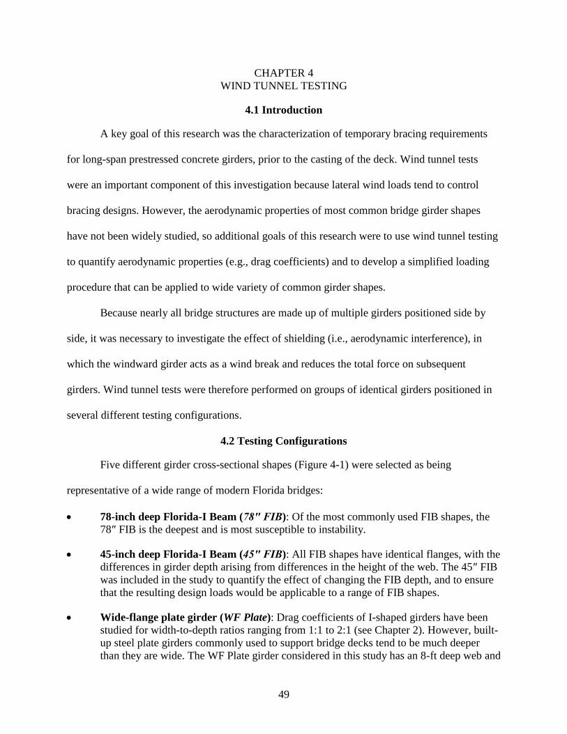
49
CHAPTER 4
WIND TUNNEL TESTING
4.1 Introduction
A key goal of this research was the characterization of temporary bracing requirements
for long-span prestressed concrete girders, prior to the casting of the deck. Wind tunnel tests
were an important component of this investigation because lateral wind loads tend to control
bracing designs. However, the aerodynamic properties of most common bridge girder shapes
have not been widely studied, so additional goals of this research were to use wind tunnel testing
to quantify aerodynamic properties (e.g., drag coefficients) and to develop a simplified loading
procedure that can be applied to wide variety of common girder shapes.
Because nearly all bridge structures are made up of multiple girders positioned side by
side, it was necessary to investigate the effect of shielding (i.e., aerodynamic interference), in
which the windward girder acts as a wind break and reduces the total force on subsequent
girders. Wind tunnel tests were therefore performed on groups of identical girders positioned in
several different testing configurations.
4.2 Testing Configurations
Five different girder cross-sectional shapes (Figure 4-1) were selected as being
representative of a wide range of modern Florida bridges:
78-inch deep Florida-I Beam (78″ FIB): Of the most commonly used FIB shapes, the
78″ FIB is the deepest and is most susceptible to instability.
45-inch deep Florida-I Beam (45″ FIB): All FIB shapes have identical flanges, with the
differences in girder depth arising from differences in the height of the web. The 45″ FIB
was included in the study to quantify the effect of changing the FIB depth, and to ensure
that the resulting design loads would be applicable to a range of FIB shapes.
Wide-flange plate girder (WF Plate): Drag coefficients of I-shaped girders have been
studied for width-to-depth ratios ranging from 1:1 to 2:1 (see Chapter 2). However, built-
up steel plate girders commonly used to support bridge decks tend to be much deeper
than they are wide. The WF Plate girder considered in this study has an 8-ft deep web and
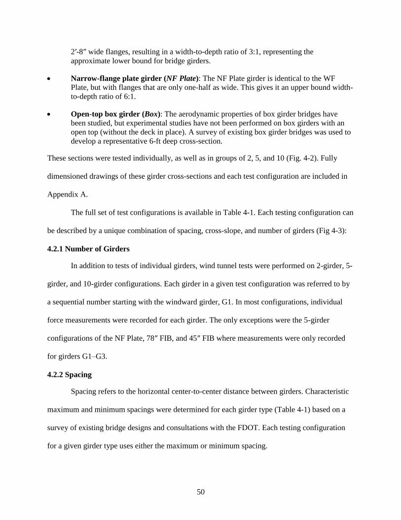
50
2′-8″ wide flanges, resulting in a width-to-depth ratio of 3:1, representing the
approximate lower bound for bridge girders.
Narrow-flange plate girder (NF Plate): The NF Plate girder is identical to the WF
Plate, but with flanges that are only one-half as wide. This gives it an upper bound width-
to-depth ratio of 6:1.
Open-top box girder (Box): The aerodynamic properties of box girder bridges have
been studied, but experimental studies have not been performed on box girders with an
open top (without the deck in place). A survey of existing box girder bridges was used to
develop a representative 6-ft deep cross-section.
These sections were tested individually, as well as in groups of 2, 5, and 10 (Fig. 4-2). Fully
dimensioned drawings of these girder cross-sections and each test configuration are included in
Appendix A.
The full set of test configurations is available in Table 4-1. Each testing configuration can
be described by a unique combination of spacing, cross-slope, and number of girders (Fig 4-3):
4.2.1 Number of Girders
In addition to tests of individual girders, wind tunnel tests were performed on 2-girder, 5-
girder, and 10-girder configurations. Each girder in a given test configuration was referred to by
a sequential number starting with the windward girder, G1. In most configurations, individual
force measurements were recorded for each girder. The only exceptions were the 5-girder
configurations of the NF Plate, 78″ FIB, and 45″ FIB where measurements were only recorded
for girders G1–G3.
4.2.2 Spacing
Spacing refers to the horizontal center-to-center distance between girders. Characteristic
maximum and minimum spacings were determined for each girder type (Table 4-1) based on a
survey of existing bridge designs and consultations with the FDOT. Each testing configuration
for a given girder type uses either the maximum or minimum spacing.
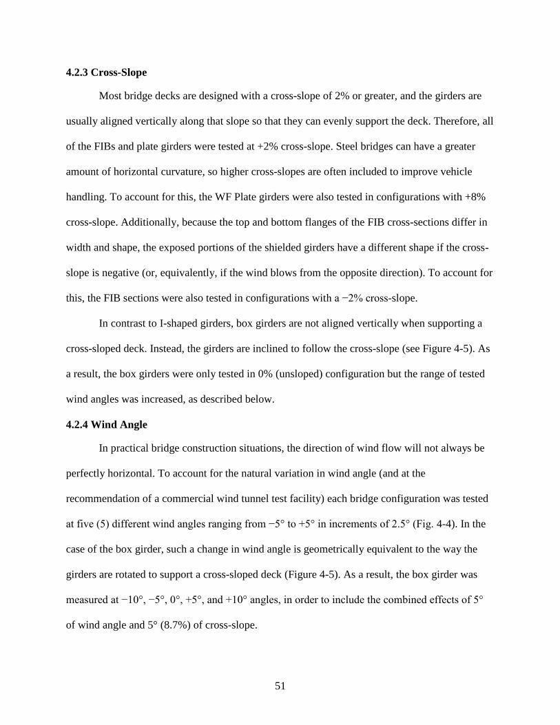
51
4.2.3 Cross-Slope
Most bridge decks are designed with a cross-slope of 2% or greater, and the girders are
usually aligned vertically along that slope so that they can evenly support the deck. Therefore, all
of the FIBs and plate girders were tested at +2% cross-slope. Steel bridges can have a greater
amount of horizontal curvature, so higher cross-slopes are often included to improve vehicle
handling. To account for this, the WF Plate girders were also tested in configurations with +8%
cross-slope. Additionally, because the top and bottom flanges of the FIB cross-sections differ in
width and shape, the exposed portions of the shielded girders have a different shape if the cross-
slope is negative (or, equivalently, if the wind blows from the opposite direction). To account for
this, the FIB sections were also tested in configurations with a −2% cross-slope.
In contrast to I-shaped girders, box girders are not aligned vertically when supporting a
cross-sloped deck. Instead, the girders are inclined to follow the cross-slope (see Figure 4-5). As
a result, the box girders were only tested in 0% (unsloped) configuration but the range of tested
wind angles was increased, as described below.
4.2.4 Wind Angle
In practical bridge construction situations, the direction of wind flow will not always be
perfectly horizontal. To account for the natural variation in wind angle (and at the
recommendation of a commercial wind tunnel test facility) each bridge configuration was tested
at five (5) different wind angles ranging from −5° to +5° in increments of 2.5° (Fig. 4-4). In the
case of the box girder, such a change in wind angle is geometrically equivalent to the way the
girders are rotated to support a cross-sloped deck (Figure 4-5). As a result, the box girder was
measured at −10°, −5°, 0°, +5°, and +10° angles, in order to include the combined effects of 5°
of wind angle and 5° (8.7%) of cross-slope.
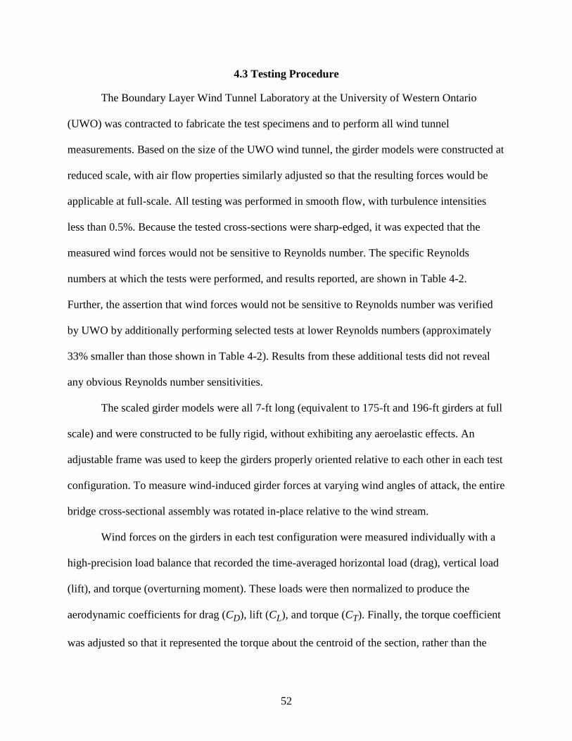
52
4.3 Testing Procedure
The Boundary Layer Wind Tunnel Laboratory at the University of Western Ontario
(UWO) was contracted to fabricate the test specimens and to perform all wind tunnel
measurements. Based on the size of the UWO wind tunnel, the girder models were constructed at
reduced scale, with air flow properties similarly adjusted so that the resulting forces would be
applicable at full-scale. All testing was performed in smooth flow, with turbulence intensities
less than 0.5%. Because the tested cross-sections were sharp-edged, it was expected that the
measured wind forces would not be sensitive to Reynolds number. The specific Reynolds
numbers at which the tests were performed, and results reported, are shown in Table 4-2.
Further, the assertion that wind forces would not be sensitive to Reynolds number was verified
by UWO by additionally performing selected tests at lower Reynolds numbers (approximately
33% smaller than those shown in Table 4-2). Results from these additional tests did not reveal
any obvious Reynolds number sensitivities.
The scaled girder models were all 7-ft long (equivalent to 175-ft and 196-ft girders at full
scale) and were constructed to be fully rigid, without exhibiting any aeroelastic effects. An
adjustable frame was used to keep the girders properly oriented relative to each other in each test
configuration. To measure wind-induced girder forces at varying wind angles of attack, the entire
bridge cross-sectional assembly was rotated in-place relative to the wind stream.
Wind forces on the girders in each test configuration were measured individually with a
high-precision load balance that recorded the time-averaged horizontal load (drag), vertical load
(lift), and torque (overturning moment). These loads were then normalized to produce the
aerodynamic coefficients for drag (CD), lift (CL), and torque (CT). Finally, the torque coefficient
was adjusted so that it represented the torque about the centroid of the section, rather than the

53
torque about the point of measurement (which was at mid-height for the I-shaped girders and at
an arbitrary point for the box girders). For additional details regarding the wind tunnel test
procedures, please see Appendix E.
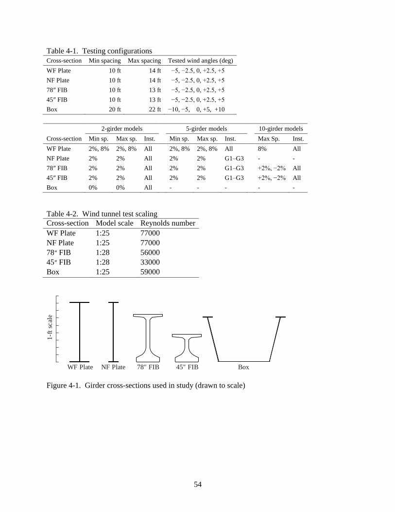
54
Table 4-1. Testing configurations
Cross-section Min spacing Max spacing Tested wind angles (deg)
WF Plate 10 ft 14 ft −5, −2.5, 0, +2.5, +5
NF Plate 10 ft 14 ft −5, −2.5, 0, +2.5, +5
78″ FIB 10 ft 13 ft −5, −2.5, 0, +2.5, +5
45″ FIB 10 ft 13 ft −5, −2.5, 0, +2.5, +5
Box 20 ft 22 ft −10, −5, 0, +5, +10
2-girder models
5-girder models
10-girder models
Cross-section Min sp. Max sp. Inst.
Min sp. Max sp. Inst.
Max Sp. Inst.
WF Plate 2%, 8% 2%, 8% All
2%, 8% 2%, 8% All
8% All
NF Plate 2% 2% All
2% 2% G1–G3
- -
78″ FIB 2% 2% All
2% 2% G1–G3
+2%, −2% All
45″ FIB 2% 2% All
2% 2% G1–G3
+2%, −2% All
Box 0% 0% All
- - -
- -
Table 4-2. Wind tunnel test scaling
Cross-section Model scale Reynolds number
WF Plate 1:25 77000
NF Plate 1:25 77000
78″ FIB 1:28 56000
45″ FIB 1:28 33000
Box 1:25 59000
WF Plate NF Plate 78" FIB 45" FIB Box
1-f
t sc
ale
Figure 4-1. Girder cross-sections used in study (drawn to scale)
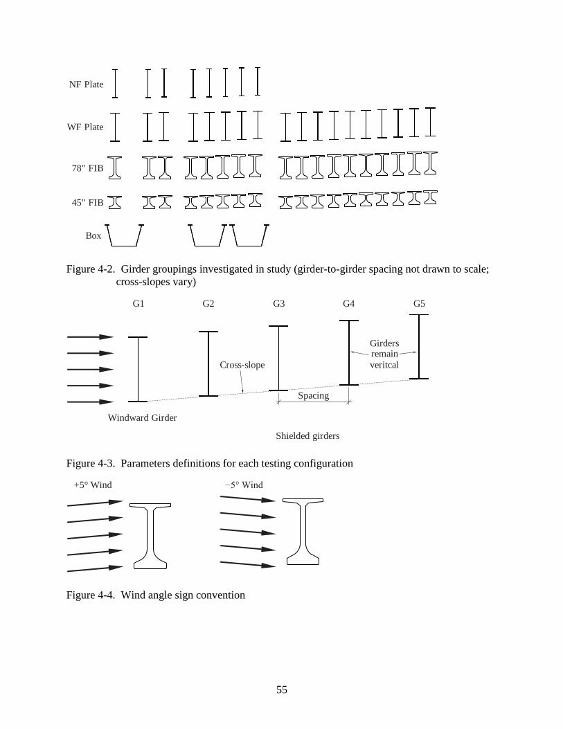
55
WF Plate
NF Plate
78" FIB
45" FIB
Box
Figure 4-2. Girder groupings investigated in study (girder-to-girder spacing not drawn to scale;
cross-slopes vary)
Girders remain
veritcal
Windward Girder
G1 G2 G3 G4 G5
Spacing
Cross-slope
Shielded girders
Figure 4-3. Parameters definitions for each testing configuration
+5° Wind −5° Wind
Figure 4-4. Wind angle sign convention
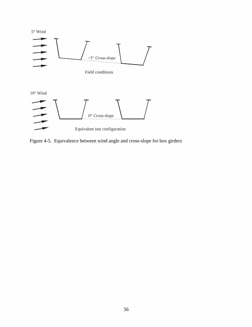
56
5° Wind
−5° Cross-slope
10° Wind
0° Cross-slope
Field conditions
Equivalent test configuration
Figure 4-5. Equivalence between wind angle and cross-slope for box girders
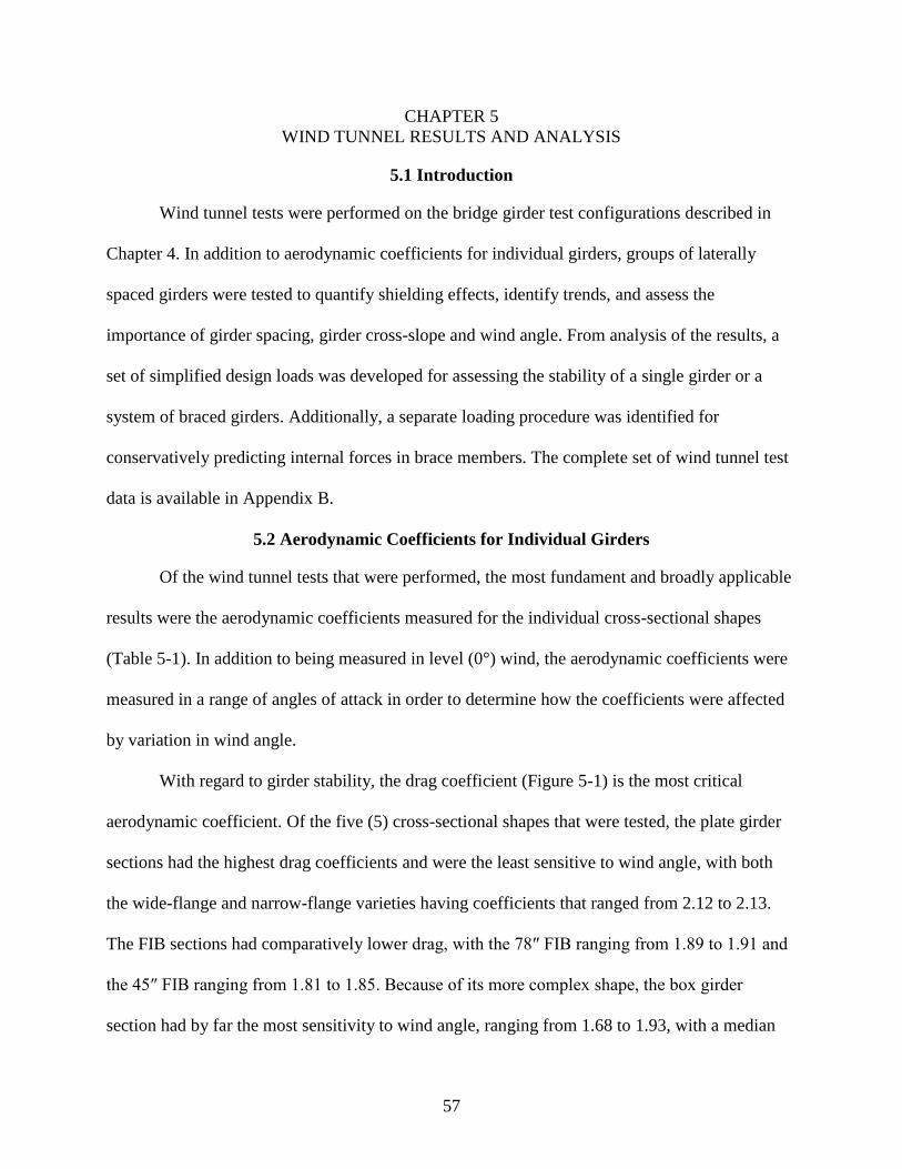
57
CHAPTER 5
WIND TUNNEL RESULTS AND ANALYSIS
5.1 Introduction
Wind tunnel tests were performed on the bridge girder test configurations described in
Chapter 4. In addition to aerodynamic coefficients for individual girders, groups of laterally
spaced girders were tested to quantify shielding effects, identify trends, and assess the
importance of girder spacing, girder cross-slope and wind angle. From analysis of the results, a
set of simplified design loads was developed for assessing the stability of a single girder or a
system of braced girders. Additionally, a separate loading procedure was identified for
conservatively predicting internal forces in brace members. The complete set of wind tunnel test
data is available in Appendix B.
5.2 Aerodynamic Coefficients for Individual Girders
Of the wind tunnel tests that were performed, the most fundament and broadly applicable
results were the aerodynamic coefficients measured for the individual cross-sectional shapes
(Table 5-1). In addition to being measured in level (0°) wind, the aerodynamic coefficients were
measured in a range of angles of attack in order to determine how the coefficients were affected
by variation in wind angle.
With regard to girder stability, the drag coefficient (Figure 5-1) is the most critical
aerodynamic coefficient. Of the five (5) cross-sectional shapes that were tested, the plate girder
sections had the highest drag coefficients and were the least sensitive to wind angle, with both
the wide-flange and narrow-flange varieties having coefficients that ranged from 2.12 to 2.13.
The FIB sections had comparatively lower drag, with the 78″ FIB ranging from 1.89 to 1.91 and
the 45″ FIB ranging from 1.81 to 1.85. Because of its more complex shape, the box girder
section had by far the most sensitivity to wind angle, ranging from 1.68 to 1.93, with a median
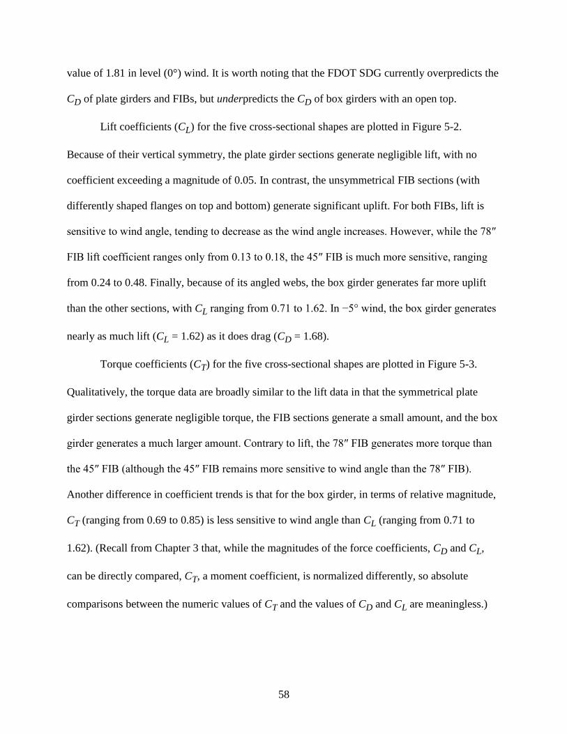
58
value of 1.81 in level (0°) wind. It is worth noting that the FDOT SDG currently overpredicts the
CD of plate girders and FIBs, but underpredicts the CD of box girders with an open top.
Lift coefficients (CL) for the five cross-sectional shapes are plotted in Figure 5-2.
Because of their vertical symmetry, the plate girder sections generate negligible lift, with no
coefficient exceeding a magnitude of 0.05. In contrast, the unsymmetrical FIB sections (with
differently shaped flanges on top and bottom) generate significant uplift. For both FIBs, lift is
sensitive to wind angle, tending to decrease as the wind angle increases. However, while the 78″
FIB lift coefficient ranges only from 0.13 to 0.18, the 45″ FIB is much more sensitive, ranging
from 0.24 to 0.48. Finally, because of its angled webs, the box girder generates far more uplift
than the other sections, with CL ranging from 0.71 to 1.62. In −5° wind, the box girder generates
nearly as much lift (CL = 1.62) as it does drag (CD = 1.68).
Torque coefficients (CT) for the five cross-sectional shapes are plotted in Figure 5-3.
Qualitatively, the torque data are broadly similar to the lift data in that the symmetrical plate
girder sections generate negligible torque, the FIB sections generate a small amount, and the box
girder generates a much larger amount. Contrary to lift, the 78″ FIB generates more torque than
the 45″ FIB (although the 45″ FIB remains more sensitive to wind angle than the 78″ FIB).
Another difference in coefficient trends is that for the box girder, in terms of relative magnitude,
CT (ranging from 0.69 to 0.85) is less sensitive to wind angle than CL (ranging from 0.71 to
1.62). (Recall from Chapter 3 that, while the magnitudes of the force coefficients, CD and CL,
can be directly compared, CT, a moment coefficient, is normalized differently, so absolute
comparisons between the numeric values of CT and the values of CD and CL are meaningless.)
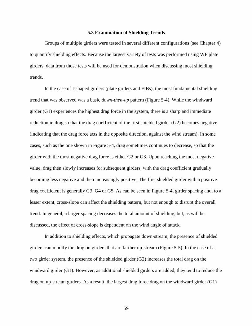
59
5.3 Examination of Shielding Trends
Groups of multiple girders were tested in several different configurations (see Chapter 4)
to quantify shielding effects. Because the largest variety of tests was performed using WF plate
girders, data from those tests will be used for demonstration when discussing most shielding
trends.
In the case of I-shaped girders (plate girders and FIBs), the most fundamental shielding
trend that was observed was a basic down-then-up pattern (Figure 5-4). While the windward
girder (G1) experiences the highest drag force in the system, there is a sharp and immediate
reduction in drag so that the drag coefficient of the first shielded girder (G2) becomes negative
(indicating that the drag force acts in the opposite direction, against the wind stream). In some
cases, such as the one shown in Figure 5-4, drag sometimes continues to decrease, so that the
girder with the most negative drag force is either G2 or G3. Upon reaching the most negative
value, drag then slowly increases for subsequent girders, with the drag coefficient gradually
becoming less negative and then increasingly positive. The first shielded girder with a positive
drag coefficient is generally G3, G4 or G5. As can be seen in Figure 5-4, girder spacing and, to a
lesser extent, cross-slope can affect the shielding pattern, but not enough to disrupt the overall
trend. In general, a larger spacing decreases the total amount of shielding, but, as will be
discussed, the effect of cross-slope is dependent on the wind angle of attack.
In addition to shielding effects, which propagate down-stream, the presence of shielded
girders can modify the drag on girders that are farther up-stream (Figure 5-5). In the case of a
two girder system, the presence of the shielded girder (G2) increases the total drag on the
windward girder (G1). However, as additional shielded girders are added, they tend to reduce the
drag on up-stream girders. As a result, the largest drag force drag on the windward girder (G1)
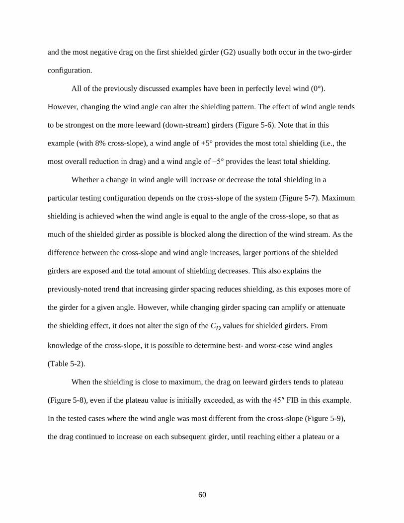
60
and the most negative drag on the first shielded girder (G2) usually both occur in the two-girder
configuration.
All of the previously discussed examples have been in perfectly level wind (0°).
However, changing the wind angle can alter the shielding pattern. The effect of wind angle tends
to be strongest on the more leeward (down-stream) girders (Figure 5-6). Note that in this
example (with 8% cross-slope), a wind angle of +5° provides the most total shielding (i.e., the
most overall reduction in drag) and a wind angle of −5° provides the least total shielding.
Whether a change in wind angle will increase or decrease the total shielding in a
particular testing configuration depends on the cross-slope of the system (Figure 5-7). Maximum
shielding is achieved when the wind angle is equal to the angle of the cross-slope, so that as
much of the shielded girder as possible is blocked along the direction of the wind stream. As the
difference between the cross-slope and wind angle increases, larger portions of the shielded
girders are exposed and the total amount of shielding decreases. This also explains the
previously-noted trend that increasing girder spacing reduces shielding, as this exposes more of
the girder for a given angle. However, while changing girder spacing can amplify or attenuate
the shielding effect, it does not alter the sign of the CD values for shielded girders. From
knowledge of the cross-slope, it is possible to determine best- and worst-case wind angles
(Table 5-2).
When the shielding is close to maximum, the drag on leeward girders tends to plateau
(Figure 5-8), even if the plateau value is initially exceeded, as with the 45″ FIB in this example.
In the tested cases where the wind angle was most different from the cross-slope (Figure 5-9),
the drag continued to increase on each subsequent girder, until reaching either a plateau or a
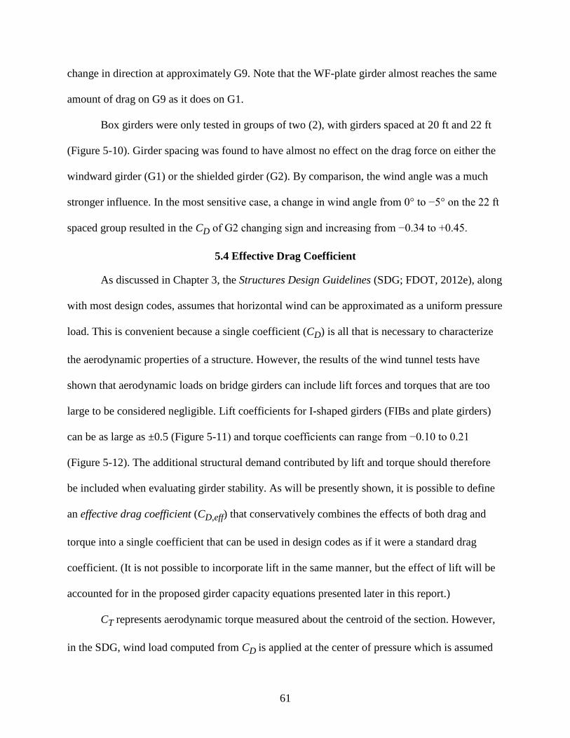
61
change in direction at approximately G9. Note that the WF-plate girder almost reaches the same
amount of drag on G9 as it does on G1.
Box girders were only tested in groups of two (2), with girders spaced at 20 ft and 22 ft
(Figure 5-10). Girder spacing was found to have almost no effect on the drag force on either the
windward girder (G1) or the shielded girder (G2). By comparison, the wind angle was a much
stronger influence. In the most sensitive case, a change in wind angle from 0° to −5° on the 22 ft
spaced group resulted in the CD of G2 changing sign and increasing from −0.34 to +0.45.
5.4 Effective Drag Coefficient
As discussed in Chapter 3, the Structures Design Guidelines (SDG; FDOT, 2012e), along
with most design codes, assumes that horizontal wind can be approximated as a uniform pressure
load. This is convenient because a single coefficient (CD) is all that is necessary to characterize
the aerodynamic properties of a structure. However, the results of the wind tunnel tests have
shown that aerodynamic loads on bridge girders can include lift forces and torques that are too
large to be considered negligible. Lift coefficients for I-shaped girders (FIBs and plate girders)
can be as large as ±0.5 (Figure 5-11) and torque coefficients can range from −0.10 to 0.21
(Figure 5-12). The additional structural demand contributed by lift and torque should therefore
be included when evaluating girder stability. As will be presently shown, it is possible to define
an effective drag coefficient (CD,eff) that conservatively combines the effects of both drag and
torque into a single coefficient that can be used in design codes as if it were a standard drag
coefficient. (It is not possible to incorporate lift in the same manner, but the effect of lift will be
accounted for in the proposed girder capacity equations presented later in this report.)
CT represents aerodynamic torque measured about the centroid of the section. However,
in the SDG, wind load computed from CD is applied at the center of pressure which is assumed
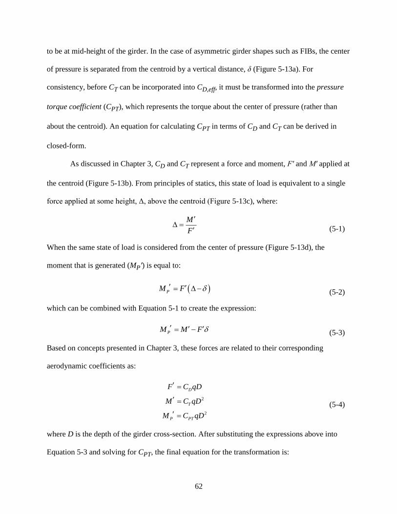
62
to be at mid-height of the girder. In the case of asymmetric girder shapes such as FIBs, the center
of pressure is separated from the centroid by a vertical distance, δ (Figure 5-13a). For
consistency, before CT can be incorporated into CD,eff, it must be transformed into the pressure
torque coefficient (CPT), which represents the torque about the center of pressure (rather than
about the centroid). An equation for calculating CPT in terms of CD and CT can be derived in
closed-form.
As discussed in Chapter 3, CD and CT represent a force and moment, F′ and M′ applied at
the centroid (Figure 5-13b). From principles of statics, this state of load is equivalent to a single
force applied at some height, Δ, above the centroid (Figure 5-13c), where:
M
F
(5-1)
When the same state of load is considered from the center of pressure (Figure 5-13d), the
moment that is generated (MP′) is equal to:
PM F (5-2)
which can be combined with Equation 5-1 to create the expression:
PM M F (5-3)
Based on concepts presented in Chapter 3, these forces are related to their corresponding
aerodynamic coefficients as:
2
2
D
T
P PT
F C qD
M C qD
M C qD
(5-4)
where D is the depth of the girder cross-section. After substituting the expressions above into
Equation 5-3 and solving for CPT, the final equation for the transformation is:
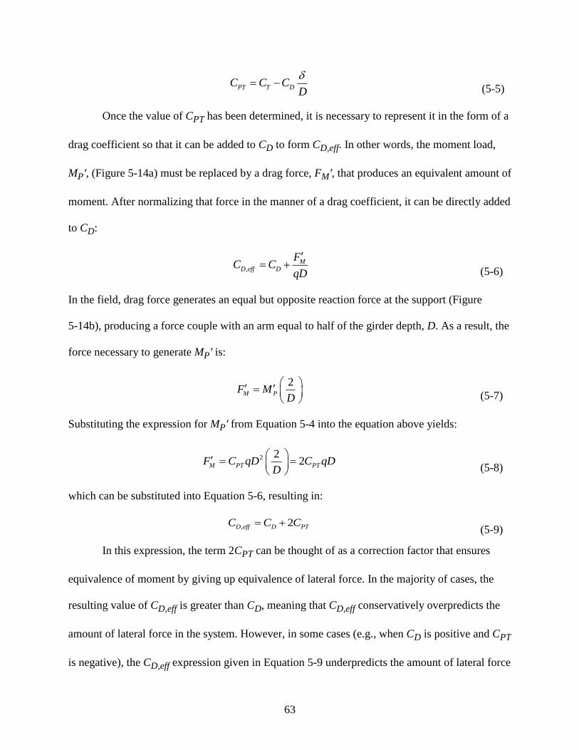
63
PT T DC C CD
(5-5)
Once the value of CPT has been determined, it is necessary to represent it in the form of a
drag coefficient so that it can be added to CD to form CD,eff. In other words, the moment load,
MP′, (Figure 5-14a) must be replaced by a drag force, FM′, that produces an equivalent amount of
moment. After normalizing that force in the manner of a drag coefficient, it can be directly added
to CD:
,M
D eff D
FC C
qD
(5-6)
In the field, drag force generates an equal but opposite reaction force at the support (Figure
5-14b), producing a force couple with an arm equal to half of the girder depth, D. As a result, the
force necessary to generate MP′ is:
2M PF M
D
(5-7)
Substituting the expression for MP′ from Equation 5-4 into the equation above yields:
2 22M PT PTF C qD C qD
D
(5-8)
which can be substituted into Equation 5-6, resulting in:
, 2D eff D PTC C C (5-9)
In this expression, the term 2CPT can be thought of as a correction factor that ensures
equivalence of moment by giving up equivalence of lateral force. In the majority of cases, the
resulting value of CD,eff is greater than CD, meaning that CD,eff conservatively overpredicts the
amount of lateral force in the system. However, in some cases (e.g., when CD is positive and CPT
is negative), the CD,eff expression given in Equation 5-9 underpredicts the amount of lateral force
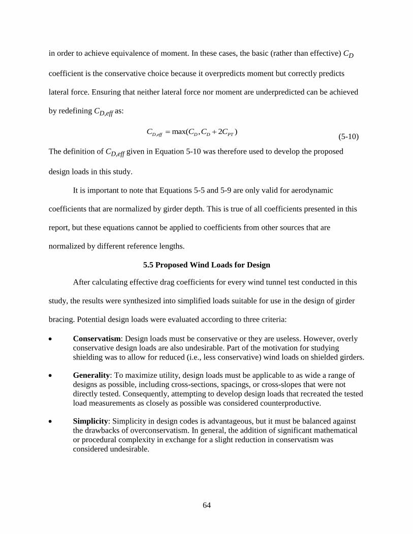
64
in order to achieve equivalence of moment. In these cases, the basic (rather than effective) CD
coefficient is the conservative choice because it overpredicts moment but correctly predicts
lateral force. Ensuring that neither lateral force nor moment are underpredicted can be achieved
by redefining CD,eff as:
, max( , 2 )D eff D D PTC C C C (5-10)
The definition of CD,eff given in Equation 5-10 was therefore used to develop the proposed
design loads in this study.
It is important to note that Equations 5-5 and 5-9 are only valid for aerodynamic
coefficients that are normalized by girder depth. This is true of all coefficients presented in this
report, but these equations cannot be applied to coefficients from other sources that are
normalized by different reference lengths.
5.5 Proposed Wind Loads for Design
After calculating effective drag coefficients for every wind tunnel test conducted in this
study, the results were synthesized into simplified loads suitable for use in the design of girder
bracing. Potential design loads were evaluated according to three criteria:
Conservatism: Design loads must be conservative or they are useless. However, overly
conservative design loads are also undesirable. Part of the motivation for studying
shielding was to allow for reduced (i.e., less conservative) wind loads on shielded girders.
Generality: To maximize utility, design loads must be applicable to as wide a range of
designs as possible, including cross-sections, spacings, or cross-slopes that were not
directly tested. Consequently, attempting to develop design loads that recreated the tested
load measurements as closely as possible was considered counterproductive.
Simplicity: Simplicity in design codes is advantageous, but it must be balanced against
the drawbacks of overconservatism. In general, the addition of significant mathematical
or procedural complexity in exchange for a slight reduction in conservatism was
considered undesirable.
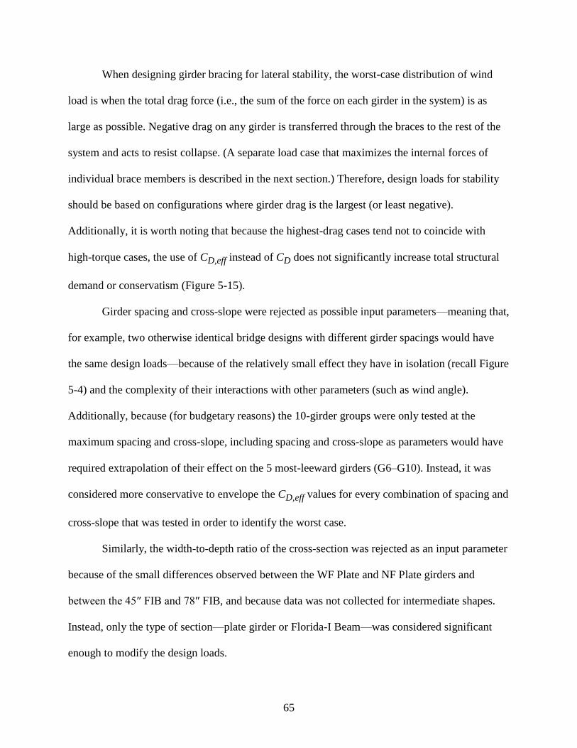
65
When designing girder bracing for lateral stability, the worst-case distribution of wind
load is when the total drag force (i.e., the sum of the force on each girder in the system) is as
large as possible. Negative drag on any girder is transferred through the braces to the rest of the
system and acts to resist collapse. (A separate load case that maximizes the internal forces of
individual brace members is described in the next section.) Therefore, design loads for stability
should be based on configurations where girder drag is the largest (or least negative).
Additionally, it is worth noting that because the highest-drag cases tend not to coincide with
high-torque cases, the use of CD,eff instead of CD does not significantly increase total structural
demand or conservatism (Figure 5-15).
Girder spacing and cross-slope were rejected as possible input parameters—meaning that,
for example, two otherwise identical bridge designs with different girder spacings would have
the same design loads—because of the relatively small effect they have in isolation (recall Figure
5-4) and the complexity of their interactions with other parameters (such as wind angle).
Additionally, because (for budgetary reasons) the 10-girder groups were only tested at the
maximum spacing and cross-slope, including spacing and cross-slope as parameters would have
required extrapolation of their effect on the 5 most-leeward girders (G6–G10). Instead, it was
considered more conservative to envelope the CD,eff values for every combination of spacing and
cross-slope that was tested in order to identify the worst case.
Similarly, the width-to-depth ratio of the cross-section was rejected as an input parameter
because of the small differences observed between the WF Plate and NF Plate girders and
between the 45″ FIB and 78″ FIB, and because data was not collected for intermediate shapes.
Instead, only the type of section—plate girder or Florida-I Beam—was considered significant
enough to modify the design loads.
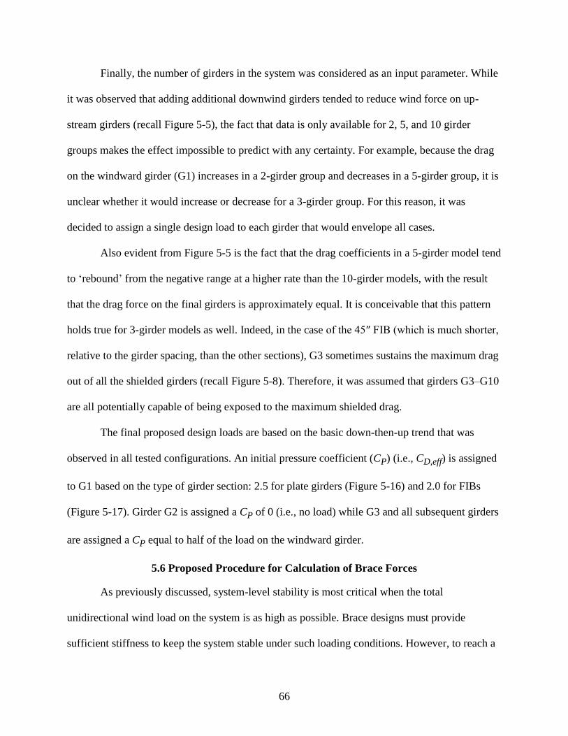
66
Finally, the number of girders in the system was considered as an input parameter. While
it was observed that adding additional downwind girders tended to reduce wind force on up-
stream girders (recall Figure 5-5), the fact that data is only available for 2, 5, and 10 girder
groups makes the effect impossible to predict with any certainty. For example, because the drag
on the windward girder (G1) increases in a 2-girder group and decreases in a 5-girder group, it is
unclear whether it would increase or decrease for a 3-girder group. For this reason, it was
decided to assign a single design load to each girder that would envelope all cases.
Also evident from Figure 5-5 is the fact that the drag coefficients in a 5-girder model tend
to ‘rebound’ from the negative range at a higher rate than the 10-girder models, with the result
that the drag force on the final girders is approximately equal. It is conceivable that this pattern
holds true for 3-girder models as well. Indeed, in the case of the 45″ FIB (which is much shorter,
relative to the girder spacing, than the other sections), G3 sometimes sustains the maximum drag
out of all the shielded girders (recall Figure 5-8). Therefore, it was assumed that girders G3–G10
are all potentially capable of being exposed to the maximum shielded drag.
The final proposed design loads are based on the basic down-then-up trend that was
observed in all tested configurations. An initial pressure coefficient (CP) (i.e., CD,eff) is assigned
to G1 based on the type of girder section: 2.5 for plate girders (Figure 5-16) and 2.0 for FIBs
(Figure 5-17). Girder G2 is assigned a CP of 0 (i.e., no load) while G3 and all subsequent girders
are assigned a CP equal to half of the load on the windward girder.
5.6 Proposed Procedure for Calculation of Brace Forces
As previously discussed, system-level stability is most critical when the total
unidirectional wind load on the system is as high as possible. Brace designs must provide
sufficient stiffness to keep the system stable under such loading conditions. However, to reach a
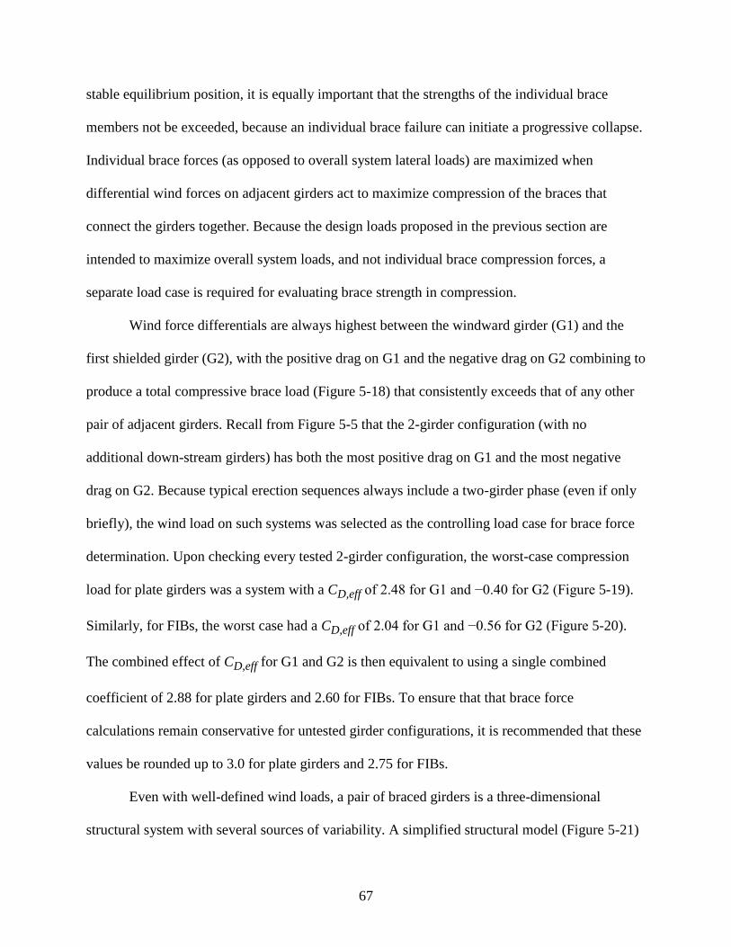
67
stable equilibrium position, it is equally important that the strengths of the individual brace
members not be exceeded, because an individual brace failure can initiate a progressive collapse.
Individual brace forces (as opposed to overall system lateral loads) are maximized when
differential wind forces on adjacent girders act to maximize compression of the braces that
connect the girders together. Because the design loads proposed in the previous section are
intended to maximize overall system loads, and not individual brace compression forces, a
separate load case is required for evaluating brace strength in compression.
Wind force differentials are always highest between the windward girder (G1) and the
first shielded girder (G2), with the positive drag on G1 and the negative drag on G2 combining to
produce a total compressive brace load (Figure 5-18) that consistently exceeds that of any other
pair of adjacent girders. Recall from Figure 5-5 that the 2-girder configuration (with no
additional down-stream girders) has both the most positive drag on G1 and the most negative
drag on G2. Because typical erection sequences always include a two-girder phase (even if only
briefly), the wind load on such systems was selected as the controlling load case for brace force
determination. Upon checking every tested 2-girder configuration, the worst-case compression
load for plate girders was a system with a CD,eff of 2.48 for G1 and −0.40 for G2 (Figure 5-19).
Similarly, for FIBs, the worst case had a CD,eff of 2.04 for G1 and −0.56 for G2 (Figure 5-20).
The combined effect of CD,eff for G1 and G2 is then equivalent to using a single combined
coefficient of 2.88 for plate girders and 2.60 for FIBs. To ensure that that brace force
calculations remain conservative for untested girder configurations, it is recommended that these
values be rounded up to 3.0 for plate girders and 2.75 for FIBs.
Even with well-defined wind loads, a pair of braced girders is a three-dimensional
structural system with several sources of variability. A simplified structural model (Figure 5-21)
68
is therefore proposed for conservative determination of brace forces using the loads described
above. This approach is not restricted to any particular brace configuration: the core of the
approach is a structural model of the brace, the configuration and implementation of which is left
to the judgment of the Engineer of Record. Fixed boundary conditions are applied at every node
where the brace connects to G2, while rigid links are used to link all of the G1 connection nodes
to a pin located at the base of G1. An additional rigid link connects the base pin to the center of
pressure where the total tributary wind load is applied as a single horizontal force.
In the field, the connections between the brace elements and the girders are likely to be
neither perfectly fixed nor perfectly pinned, but rather achieve some intermediate level of
moment transfer. If desired and appropriate, brace elements may include partial end-releases at
the girder connection points. This can lessen the resulting brace forces somewhat. However, it is
important not to underpredict the amount of fixity in the connections or unconservative results
may be obtained. Given the significant amount of uncertainty that is generally involved in such
determinations, it is recommended that full fixity be provided in the model unless reliable
partially-restrained connection information is available.
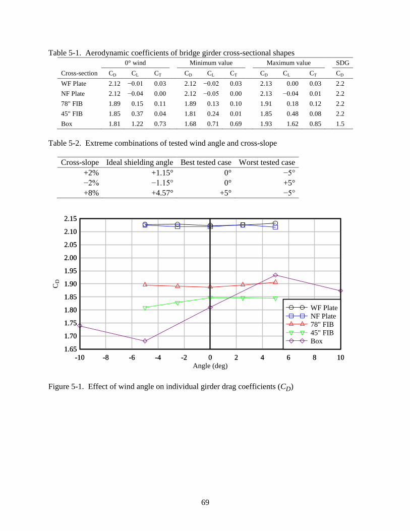
69
Table 5-1. Aerodynamic coefficients of bridge girder cross-sectional shapes
0° wind Minimum value Maximum value SDG
Cross-section +CD +CL +CT +CD +CL +CT +CD +CL +CT CD
WF Plate +2.12 −0.01 +0.03 +2.12 −0.02 +0.03 +2.13 ++0.00 +0.03 2.2
NF Plate +2.12 −0.04 +0.00 +2.12 −0.05 +0.00 +2.13 +−0.04 +0.01 2.2
78" FIB +1.89 +0.15 +0.11 +1.89 +0.13 +0.10 +1.91 ++0.18 +0.12 2.2
45" FIB +1.85 +0.37 +0.04 +1.81 +0.24 +0.01 +1.85 ++0.48 +0.08 2.2
Box +1.81 +1.22 +0.73 +1.68 +0.71 +0.69 +1.93 ++1.62 +0.85 1.5
Table 5-2. Extreme combinations of tested wind angle and cross-slope
Cross-slope Ideal shielding angle Best tested case Worst tested case
+2% +1.15° +0° −5°
−2% −1.15° +0° +5°
+8% +4.57° +5° −5°
Figure 5-1. Effect of wind angle on individual girder drag coefficients (CD)
Angle (deg)
CD
-10 -8 -6 -4 -2 0 2 4 6 8 10
1.65
1.70
1.75
1.80
1.85
1.90
1.95
2.00
2.05
2.10
2.15
-10 -8 -6 -4 -2 0 2 4 6 8 10
1.65
1.70
1.75
1.80
1.85
1.90
1.95
2.00
2.05
2.10
2.15
WF Plate
NF Plate
78" FIB
45" FIB
Box
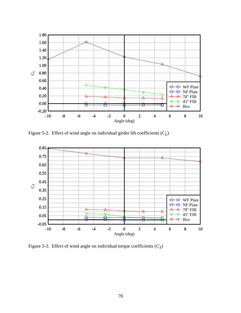
70
Figure 5-2. Effect of wind angle on individual girder lift coefficients (CL)
Figure 5-3. Effect of wind angle on individual torque coefficients (CT)
Angle (deg)
CL
-10 -8 -6 -4 -2 0 2 4 6 8 10
-0.20
0.00
0.20
0.40
0.60
0.80
1.00
1.20
1.40
1.60
1.80
-10 -8 -6 -4 -2 0 2 4 6 8 10
-0.20
0.00
0.20
0.40
0.60
0.80
1.00
1.20
1.40
1.60
1.80
WF Plate
NF Plate
78" FIB
45" FIB
Box
Angle (deg)
CT
-10 -8 -6 -4 -2 0 2 4 6 8 10
-0.05
0.05
0.15
0.25
0.35
0.45
0.55
0.65
0.75
0.85
-10 -8 -6 -4 -2 0 2 4 6 8 10
-0.05
0.05
0.15
0.25
0.35
0.45
0.55
0.65
0.75
0.85
WF Plate
NF Plate
78" FIB
45" FIB
Box
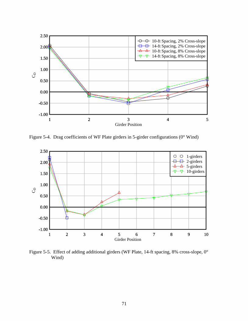
71
Figure 5-4. Drag coefficients of WF Plate girders in 5-girder configurations (0° Wind)
Figure 5-5. Effect of adding additional girders (WF Plate, 14-ft spacing, 8% cross-slope, 0°
Wind)
Girder Position
CD
1 2 3 4 5
-1.00
-0.50
0.00
0.50
1.00
1.50
2.00
2.50
1 2 3 4 5
-1.00
-0.50
0.00
0.50
1.00
1.50
2.00
2.50
10-ft Spacing, 2% Cross-slope
14-ft Spacing, 2% Cross-slope
10-ft Spacing, 8% Cross-slope
14-ft Spacing, 8% Cross-slope
Girder Position
CD
1 2 3 4 5 6 7 8 9 10
-1.00
-0.50
0.00
0.50
1.00
1.50
2.00
2.50
1 2 3 4 5 6 7 8 9 10
-1.00
-0.50
0.00
0.50
1.00
1.50
2.00
2.50
1-girders
2-girders
5-girders
10-girders
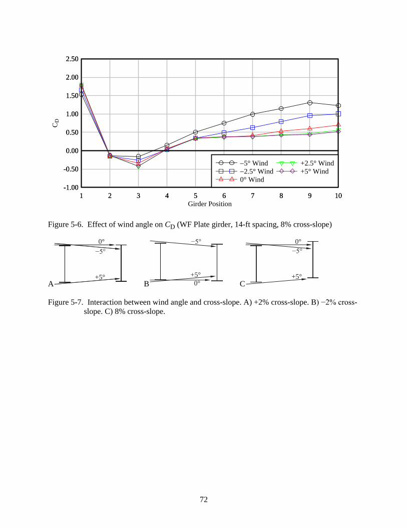
72
Figure 5-6. Effect of wind angle on CD (WF Plate girder, 14-ft spacing, 8% cross-slope)
A
−5°
+5°
0°
B
−5°
0°
+5°
C+5°
−5°
0°
Figure 5-7. Interaction between wind angle and cross-slope. A) +2% cross-slope. B) −2% cross-
slope. C) 8% cross-slope.
Girder Position
CD
1 2 3 4 5 6 7 8 9 10
-1.00
-0.50
0.00
0.50
1.00
1.50
2.00
2.50
1 2 3 4 5 6 7 8 9 10
-1.00
-0.50
0.00
0.50
1.00
1.50
2.00
2.50
5° Wind
2.5° Wind
0° Wind
+2.5° Wind
+5° Wind
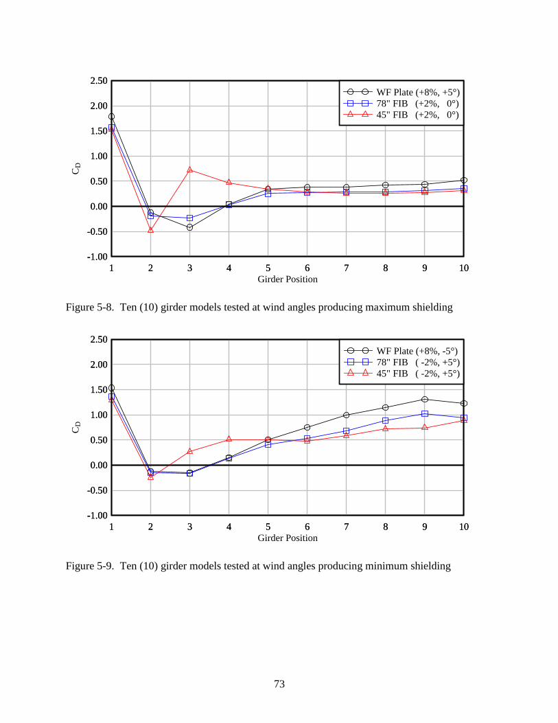
73
Figure 5-8. Ten (10) girder models tested at wind angles producing maximum shielding
Figure 5-9. Ten (10) girder models tested at wind angles producing minimum shielding
Girder Position
CD
1 2 3 4 5 6 7 8 9 10
-1.00
-0.50
0.00
0.50
1.00
1.50
2.00
2.50
1 2 3 4 5 6 7 8 9 10
-1.00
-0.50
0.00
0.50
1.00
1.50
2.00
2.50
WF Plate (+8%, +5°)
78" FIB (+2%, 0°)
45" FIB (+2%, 0°)
Girder Position
CD
1 2 3 4 5 6 7 8 9 10
-1.00
-0.50
0.00
0.50
1.00
1.50
2.00
2.50
1 2 3 4 5 6 7 8 9 10
-1.00
-0.50
0.00
0.50
1.00
1.50
2.00
2.50
WF Plate (+8%, -5°)
78" FIB ( -2%, +5°)
45" FIB ( -2%, +5°)
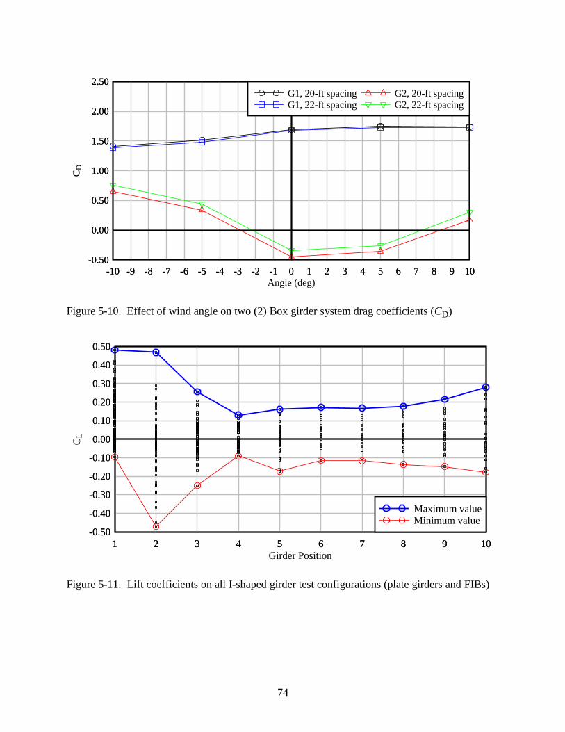
74
Figure 5-10. Effect of wind angle on two (2) Box girder system drag coefficients (CD)
Figure 5-11. Lift coefficients on all I-shaped girder test configurations (plate girders and FIBs)
Angle (deg)
CD
-10 -9 -8 -7 -6 -5 -4 -3 -2 -1 0 1 2 3 4 5 6 7 8 9 10
-0.50
0.00
0.50
1.00
1.50
2.00
2.50
-10 -9 -8 -7 -6 -5 -4 -3 -2 -1 0 1 2 3 4 5 6 7 8 9 10
-0.50
0.00
0.50
1.00
1.50
2.00
2.50
G1, 20-ft spacing
G1, 22-ft spacing
G2, 20-ft spacing
G2, 22-ft spacing
Girder Position
CL
1 2 3 4 5 6 7 8 9 10
-0.50
-0.40
-0.30
-0.20
-0.10
0.00
0.10
0.20
0.30
0.40
0.50
1 2 3 4 5 6 7 8 9 10
-0.50
-0.40
-0.30
-0.20
-0.10
0.00
0.10
0.20
0.30
0.40
0.50
Maximum value
Minimum value
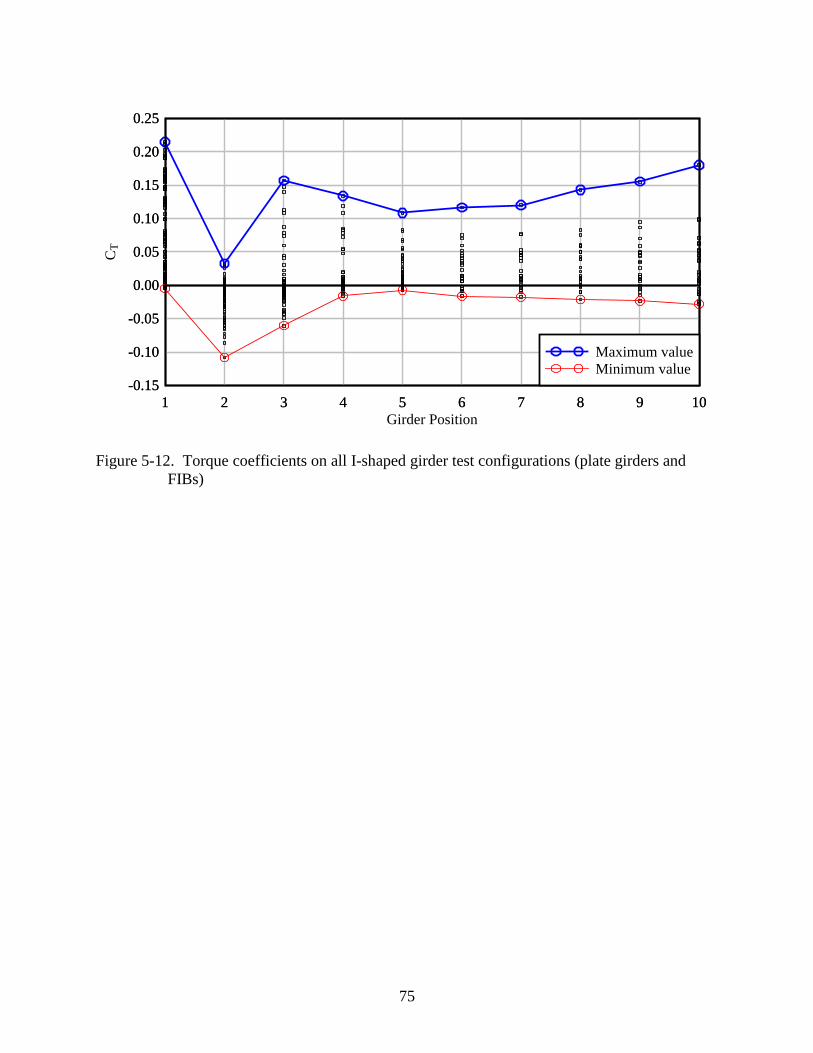
75
Figure 5-12. Torque coefficients on all I-shaped girder test configurations (plate girders and
FIBs)
Girder Position
CT
1 2 3 4 5 6 7 8 9 10
-0.15
-0.10
-0.05
0.00
0.05
0.10
0.15
0.20
0.25
1 2 3 4 5 6 7 8 9 10
-0.15
-0.10
-0.05
0.00
0.05
0.10
0.15
0.20
0.25
Maximum value
Minimum value

76
A
Center of pressure
Centroid
D
F′M′
B
C
F′
M′ =F′
F′MP′
D
Figure 5-13. Transformation of CT to CPT. A) Section dimensions. B) Force/moment pair at
section centroid. C) Equivalent elevated force. D) Force/moment pair at center of
pressure.
A
MP′
FM′
FM′ (reaction)
Bearing Pad D2
D2
B
Figure 5-14. Moment load expressed as equivalent drag force. A) Moment about center of
pressure. B) Equivalent drag force.
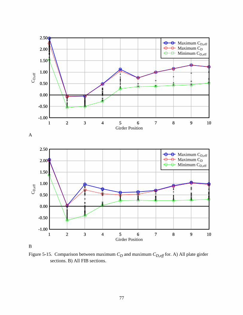
77
A
B
Figure 5-15. Comparison between maximum CD and maximum CD,eff for. A) All plate girder
sections. B) All FIB sections.
Girder Position
CD
,eff
1 2 3 4 5 6 7 8 9 10
-1.00
-0.50
0.00
0.50
1.00
1.50
2.00
2.50
1 2 3 4 5 6 7 8 9 10
-1.00
-0.50
0.00
0.50
1.00
1.50
2.00
2.50
Maximum CD,eff
Maximum CD
Minimum CD,eff
Girder Position
CD
,eff
1 2 3 4 5 6 7 8 9 10
-1.00
-0.50
0.00
0.50
1.00
1.50
2.00
2.50
1 2 3 4 5 6 7 8 9 10
-1.00
-0.50
0.00
0.50
1.00
1.50
2.00
2.50
Maximum CD,eff
Maximum CD
Minimum CD,eff
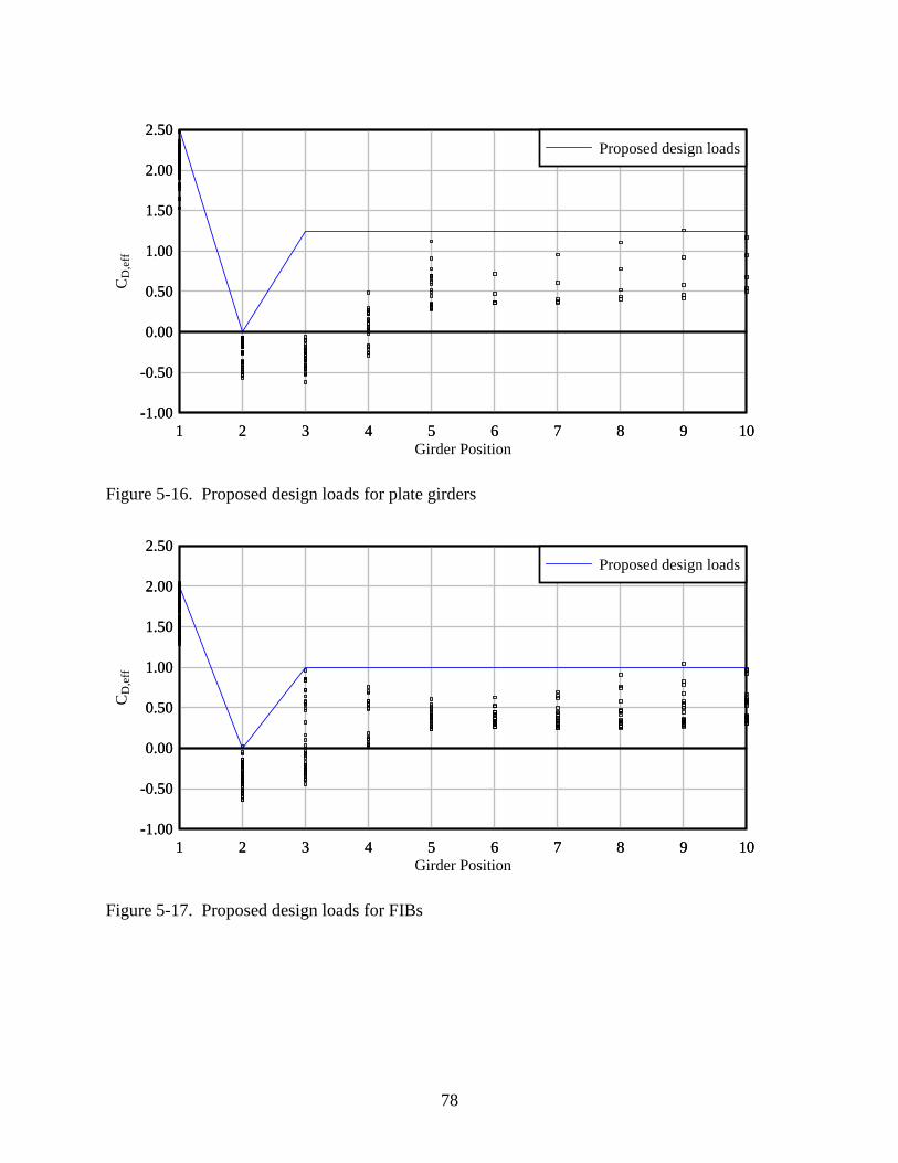
78
Figure 5-16. Proposed design loads for plate girders
Figure 5-17. Proposed design loads for FIBs
Girder Position
CD
,eff
1 2 3 4 5 6 7 8 9 10
-1.00
-0.50
0.00
0.50
1.00
1.50
2.00
2.50
1 2 3 4 5 6 7 8 9 10
-1.00
-0.50
0.00
0.50
1.00
1.50
2.00
2.50
Proposed design loads
Girder Position
CD
,eff
1 2 3 4 5 6 7 8 9 10
-1.00
-0.50
0.00
0.50
1.00
1.50
2.00
2.50
1 2 3 4 5 6 7 8 9 10
-1.00
-0.50
0.00
0.50
1.00
1.50
2.00
2.50
Proposed design loads
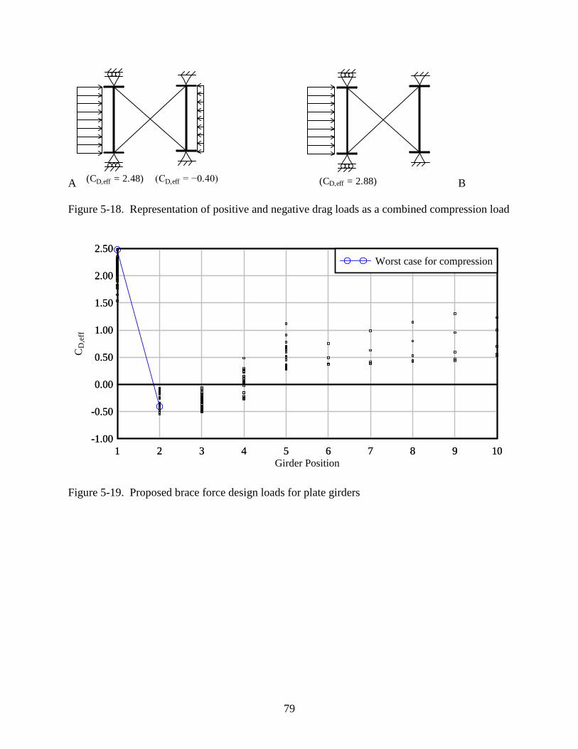
79
A (C = 2.48)D,eff (C = −0.40)D,eff (C = 2.88)D,eff B
Figure 5-18. Representation of positive and negative drag loads as a combined compression load
Figure 5-19. Proposed brace force design loads for plate girders
Girder Position
CD
,eff
1 2 3 4 5 6 7 8 9 10
-1.00
-0.50
0.00
0.50
1.00
1.50
2.00
2.50
1 2 3 4 5 6 7 8 9 10
-1.00
-0.50
0.00
0.50
1.00
1.50
2.00
2.50
Worst case for compression
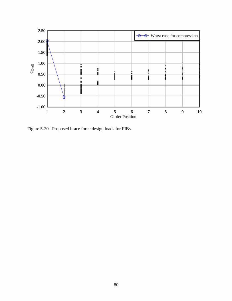
80
Figure 5-20. Proposed brace force design loads for FIBs
Girder Position
CD
,eff
1 2 3 4 5 6 7 8 9 10
-1.00
-0.50
0.00
0.50
1.00
1.50
2.00
2.50
1 2 3 4 5 6 7 8 9 10
-1.00
-0.50
0.00
0.50
1.00
1.50
2.00
2.50
Worst case for compression
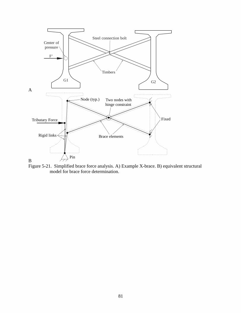
81
A
Timbers
Steel connection bolt
F′
Center of
pressure
G1 G2
BPin
Two nodes with
hinge constraint
Fixed
Brace elementsRigid links
Tributary Force
Node (typ.)
Figure 5-21. Simplified brace force analysis. A) Example X-brace. B) equivalent structural
model for brace force determination.

82
CHAPTER 6
BEARING PADS
6.1 Introduction
When analyzing the stability of girder systems, it is important to consider the support
conditions of the girders. In order to determine the support stiffness in each degree of freedom, it
is necessary to calculate bearing pad stiffness in each of four pad deformation modes: shear,
torsion, compression (axial) and rotation. While relatively simple methods are available for the
calculation of shear and torsional stiffnesses, the calculation of axial and rotational stiffnesses
requires more advanced calculation methods.
Empirical equations for calculating the compressive stiffness of a pad are available in the
literature (Gent, 2001; Stanton et al., 2008; Podolny and Muller, 1982), but they frequently
produce results that differ significantly fromeach other. One proven reliable method for
quantifying compressive pad stiffness is the finite element method, but most bridge engineers
have limited experience in modeling incompressible materials such as elastomer.
In addition to axial deformations, bearing pads are susceptible to roll rotations about two
orthogonal axes; roll about the transverse centerline (bending roll) is typically the result of the
end rotations of the girder as it bends about its major axis, while rotation about the longitudinal
centerline (overturning roll) corresponds to overturning rotations of the girder at the supports.
Estimation of these stiffnesses is often required for construction and design calculations, but
methods for calculating such stiffnesses are not comprehensively addressed in the literature. For
example, overturning roll stiffness at the supports is of particular importance during the
construction (prior to casting of the deck) of long-span prestressed concrete girder bridges, as it
can have a significant influence on the lateral stability of an unbraced girder, and is sometimes
the only source of structural resistance to overturning moments generated by lateral loads (e.g.,

83
wind) or eccentric gravity loads. Recent experimental measurements of bearing pad roll stiffness
(Consolazio et al., 2012), which extended into the nonlinear range, have provided an opportunity
to develop an empirical calculation method capable of approximating roll stiffness while
preserving nonlinear effects.
The types of bearing pads under consideration in this study consist of rectangular steel
plates separated by layers of neoprene rubber (Figure 6-1). An external neoprene cover layer,
typically thinner than the internal layers, surrounds the pad on all sides, sealing the steel
reinforcement against corrosive agents in the environment. During the vulcanization process, the
neoprene becomes fully bonded to the steel. Because the elastic modulus of the steel is so much
greater than that of the neoprene, it can be considered to be effectively rigid.
6.2 Behavior of Pads in Compression
Elastomeric rubbers, such as neoprene, are almost completely incompressible (i.e., with a
Poisson’s ratio ν > 0.49), and when subjected to a uniaxial compressive force, they tend to
expand laterally to preserve their volume. However, in a steel-reinforced bearing pad, the steel
plates are stiff enough to effectively restrain all movement of the neoprene at the steel–neoprene
interfaces. As a result, when a pad is compressed, the neoprene layers respond by bulging
outward at the edges (Figure 6-2). Restraint of this expansion by the steel plates makes the pad
much stiffer in compression than an unreinforced pad with equivalent thickness and volume of
elastomer. At extreme levels of compression, the stiffness becomes nonlinear as the bulging
displaces a significant portion of elastomer outside of the primary load path, reducing the
effective layer thickness and stiffening the pad. However, if the pad has been properly sized
according to the provisions of AASHTO (2010) or similar, then determining just the initial linear
stiffness is sufficient for most relevant bridge engineering calculations.

84
One consequence of the characteristic bulge response is an uneven distribution of
compressive stiffness throughout the pad such that local compressive stiffness at any point is a
function of the distance from the center of the pad. Near the center, there is a large amount of
surrounding rubber that must be displaced laterally in order for the neoprene layers to bulge at
the edges. In contrast, near the edges of the pad, the rubber is less confined and comparatively
little force is required for the rubber to bulge. This confinement effect can be demonstrated by
prescribing a uniform downward displacement on the top surface of a finite element model of a
layer of neoprene and plotting the distribution of the reaction forces (Figure 6-3). Because every
point on the pad is compressed (deformed) vertically the same amount, the reaction force
distribution is proportional to the distribution of local stiffness.
Gent (2001) and others have published correlations between the axial stiffness of a
bearing pad and the shape factor, S, of the internal elastomer layers of the pad. The shape factor
is a dimensionless ratio between the load area (i.e., plan-view area of the pad) and the bulge
area (i.e., the perimeter area). Most shape factor–based methods use the same basic functional
form:
21c aE E B S (6-1)
(where Ba is an empirically-determined constant) to calculate an effective elastic modulus for
compression, Ec, that incorporates the additional restraint provided by the steel reinforcement.
Stanton et al. (2008) have refined this approach, providing a method for determining Ba that
takes into account the bulk compressibility of the elastomer. In contrast, Podolny and Muller
(1982) have provided an empirical formula:
2
3axial
GAak
Ct (6-2)
85
that does not incorporate the shape factor, but does include a constant, C, that changes depending
on the aspect ratio of the pad.
6.3 Behavior of Pads in Roll Rotation
As a girder rolls, the top surface of the pad becomes angled relative to the bottom surface,
lifting upward from one side of the pad and depressing the opposite side. Because the pad is
already compressed by the weight of the girder it supports, the entire width of the pad initially
remains in contact with the girder and the initial roll stiffness of the pad is linear. However, if the
roll angle becomes large enough, the girder will begin to lift off the pad, and the roll stiffness
will become nonlinear (Figure 6-4). The critical roll angle at which this occurs is dependent on
the initial compression load. As more of the pad becomes disengaged, the roll stiffness softens
until the moment vs. rotation (angle) curve becomes horizontal (plateaus) and the girder rolls off
of the pad.
In 2012, an experimental study (Consolazio et al., 2012) demonstrated that an increase in
the initial compression load results in an approximately proportional increase in the plateau value
(while the initial roll stiffness remains essentially unaffected). Also demonstrated in the study
were the effects of the geometric orientation of the girder centerline relative to the longitudinal
centerline of the pad. Specifically, the two types of orientation angle considered were slope
(divergence of the centerlines in elevation view) and skew (divergence in plan view). It was
found that overturning roll stiffness was significantly reduced when skew was present, and that
this effect was exacerbated by the simultaneous inclusion of a non-zero slope angle. These
experimental findings confirmed results from an earlier study (Consolazio et al., 2007) in which
the interaction between skew and slope was examined analytically. The effect of slope alone
(with no skew) was less conclusive in the experimental study due to scatter in the experimental
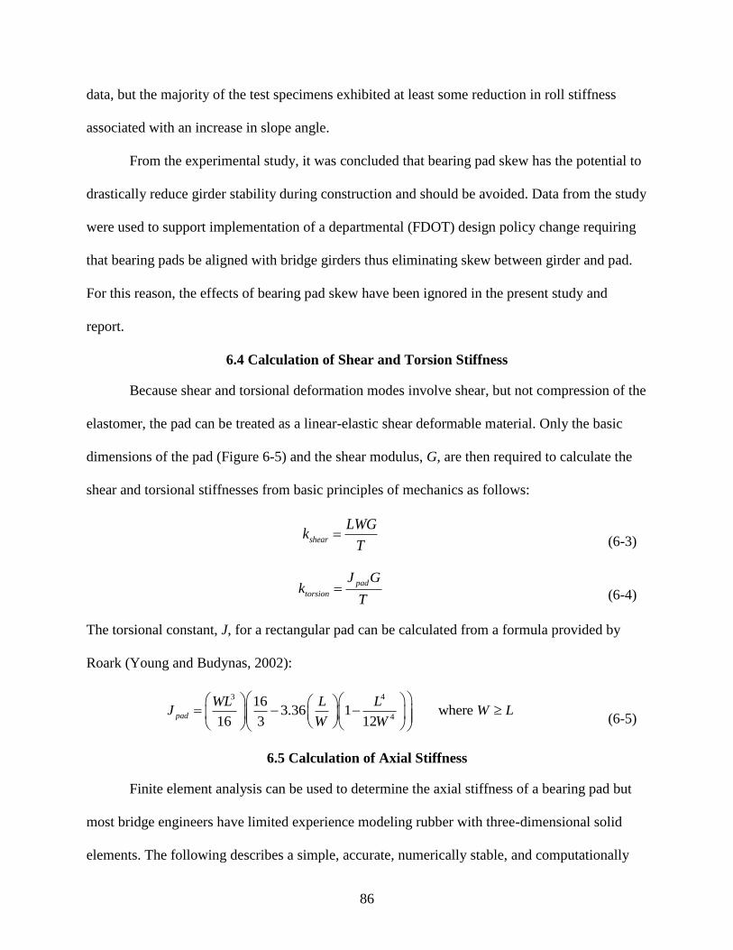
86
data, but the majority of the test specimens exhibited at least some reduction in roll stiffness
associated with an increase in slope angle.
From the experimental study, it was concluded that bearing pad skew has the potential to
drastically reduce girder stability during construction and should be avoided. Data from the study
were used to support implementation of a departmental (FDOT) design policy change requiring
that bearing pads be aligned with bridge girders thus eliminating skew between girder and pad.
For this reason, the effects of bearing pad skew have been ignored in the present study and
report.
6.4 Calculation of Shear and Torsion Stiffness
Because shear and torsional deformation modes involve shear, but not compression of the
elastomer, the pad can be treated as a linear-elastic shear deformable material. Only the basic
dimensions of the pad (Figure 6-5) and the shear modulus, G, are then required to calculate the
shear and torsional stiffnesses from basic principles of mechanics as follows:
shear
LWGk
T
(6-3)
pad
torsion
J Gk
T
(6-4)
The torsional constant, J, for a rectangular pad can be calculated from a formula provided by
Roark (Young and Budynas, 2002):
3 4
4
163.36 1 where
16 3 12pad
WL L LJ W L
W W
(6-5)
6.5 Calculation of Axial Stiffness
Finite element analysis can be used to determine the axial stiffness of a bearing pad but
most bridge engineers have limited experience modeling rubber with three-dimensional solid
elements. The following describes a simple, accurate, numerically stable, and computationally
87
efficient modeling approach for quantifying axial stiffness, without the need for specialized
material testing.
6.5.1 Stiffness of Neoprene Layers
As previously mentioned, steel reinforcing plates are stiff enough, relative to neoprene,
that they can be treated as effectively rigid. As a result, the overall axial stiffness of a pad is
equivalent to the individual stiffnesses of the neoprene layers (including the top and bottom
cover layers) combined in series (Figure 6-6). It is only necessary to model the individual
neoprene layers and then combine the results to determine the axial stiffness of the pad. Because
all internal layers typically have the same thickness, generally it will only be necessary to create
two finite element layer models—an internal layer model and a cover layer model.
6.5.2 Model Dimensions and Meshing
While it is important to include the cover layers at the top and bottom of the pad, the side
layer that surrounds the perimeter of the pad does not contribute significantly to pad stiffness and
does not need to be included in the finite element models. Instead, both layer models (internal
and cover) should have the same plan-view dimensions as the steel reinforcing plates, differing
only in thickness.
The use of tri-quadratic solid elements (e.g., 20-node or 27-node) is highly recommended
to avoid shear locking, as the higher-order shape functions employed by such elements more
naturally approximate the curvature of the elastomeric bulge. A much smaller quantity of solid
elements is then required, significantly reducing the computational burden. A mesh convergence
study has demonstrated that if 27-node solid elements are used, a layer model need only be two
elements thick, and the plan-view dimensions of the elements can be as large as 1 in. on either
side (as long as the model has a minimum subdivision of eight elements in both directions)
(Figure 6-7).

88
6.5.3 Loading and Boundary Conditions
All of the nodes on the bottom surface of each elastomer layer model should be fixed in
place, while the nodes on the top surface are constrained together into a nodal rigid body,
representing the restraint provided by the steel reinforcement (or by friction between the pad and
the girder or substructure). Application of a uniform axial pressure load of 100–200 psi is
sufficient to characterize the initial axial stiffness of typical pads.
6.5.4 Material Model
Rubbers and other incompressible materials are generally modeled as hyperelastic
materials, meaning that the mechanical properties are defined by a strain energy density function,
W(λ1, λ2, λ3), which relates the total strain energy per unit volume to the deformed state of the
material. Each hyperelastic model uses a different form of W, which is nearly always written in
terms of the principal stretch ratios, λ1, λ2, and λ3, which represent the material deformation.
Stretch is defined as the ratio of deformed length to undeformed length, so the principal stretches
can be related to the principal strains as:
1i ii i
i
L L
L
(6-6)
In most hyperelastic materials, the functional form of W is selected empirically, and
requires two or more material parameters which must be determined from experimental testing
of specially-prepared material specimens. Material testing is often not feasible for bridge design
and, in most circumstances, the only available material data for the neoprene in a bearing pad is
the shear modulus, G. In some cases, only a durometer hardness value may be available, which
can be converted into an approximate shear modulus empirically (Podolny and Muller, 1982;
AASHTO, 2010).
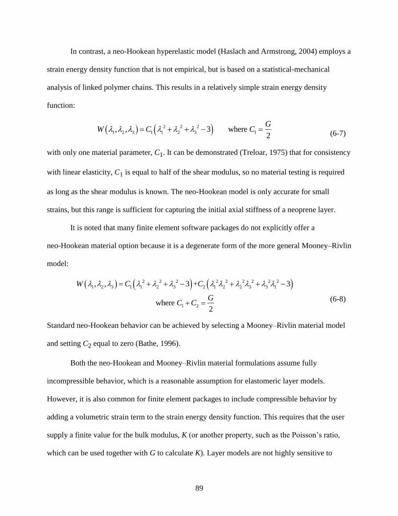
89
In contrast, a neo-Hookean hyperelastic model (Haslach and Armstrong, 2004) employs a
strain energy density function that is not empirical, but is based on a statistical-mechanical
analysis of linked polymer chains. This results in a relatively simple strain energy density
function:
2 2 2
1 2 3 1 1 2 3 1, , 3 where 2
GW C C
(6-7)
with only one material parameter, C1. It can be demonstrated (Treloar, 1975) that for consistency
with linear elasticity, C1 is equal to half of the shear modulus, so no material testing is required
as long as the shear modulus is known. The neo-Hookean model is only accurate for small
strains, but this range is sufficient for capturing the initial axial stiffness of a neoprene layer.
It is noted that many finite element software packages do not explicitly offer a
neo-Hookean material option because it is a degenerate form of the more general Mooney–Rivlin
model:
2 2 2 2 2 2 2 2 2
1 2 3 1 1 2 3 2 1 2 2 3 3 1
1 2
, , 3 + 3
where 2
W C C
GC C
(6-8)
Standard neo-Hookean behavior can be achieved by selecting a Mooney–Rivlin material model
and setting C2 equal to zero (Bathe, 1996).
Both the neo-Hookean and Mooney–Rivlin material formulations assume fully
incompressible behavior, which is a reasonable assumption for elastomeric layer models.
However, it is also common for finite element packages to include compressible behavior by
adding a volumetric strain term to the strain energy density function. This requires that the user
supply a finite value for the bulk modulus, K (or another property, such as the Poisson’s ratio,
which can be used together with G to calculate K). Layer models are not highly sensitive to
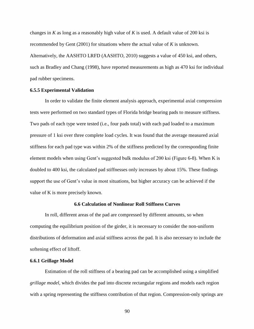
90
changes in K as long as a reasonably high value of K is used. A default value of 200 ksi is
recommended by Gent (2001) for situations where the actual value of K is unknown.
Alternatively, the AASHTO LRFD (AASHTO, 2010) suggests a value of 450 ksi, and others,
such as Bradley and Chang (1998), have reported measurements as high as 470 ksi for individual
pad rubber specimens.
6.5.5 Experimental Validation
In order to validate the finite element analysis approach, experimental axial compression
tests were performed on two standard types of Florida bridge bearing pads to measure stiffness.
Two pads of each type were tested (i.e., four pads total) with each pad loaded to a maximum
pressure of 1 ksi over three complete load cycles. It was found that the average measured axial
stiffness for each pad type was within 2% of the stiffness predicted by the corresponding finite
element models when using Gent’s suggested bulk modulus of 200 ksi (Figure 6-8). When K is
doubled to 400 ksi, the calculated pad stiffnesses only increases by about 15%. These findings
support the use of Gent’s value in most situations, but higher accuracy can be achieved if the
value of K is more precisely known.
6.6 Calculation of Nonlinear Roll Stiffness Curves
In roll, different areas of the pad are compressed by different amounts, so when
computing the equilibrium position of the girder, it is necessary to consider the non-uniform
distributions of deformation and axial stiffness across the pad. It is also necessary to include the
softening effect of liftoff.
6.6.1 Grillage Model
Estimation of the roll stiffness of a bearing pad can be accomplished using a simplified
grillage model, which divides the pad into discrete rectangular regions and models each region
with a spring representing the stiffness contribution of that region. Compression-only springs are
91
used to allow the girder to liftoff from the pad. The upper nodes of the springs are linked
together into a rigid body which represents the top surface of the pad (i.e., the surface in contact
with the girder), while the bottom nodes are fixed in place.
The grillage model must first be compressed by a uniform axial load, representing the
weight of the girder. Then an overturning moment can be applied to the top surface and a
structural analysis can be used to determine the resulting roll angle (Figure 6-9). If the
overturning moment is increased incrementally, a complete stiffness curve can be generated.
6.6.2 Spring Stiffness Distribution in Grillage Model
Several methods of distributing stiffness values to the springs in the grillage model were
considered and the resulting stiffness curves were compared to experimental roll stiffness
measurements (Consolazio et al., 2012) that were obtained for three standard FDOT pad types
(Figure 6-10), designated A, B, and C. Empirically, the best approach was found to involve the
use of a parabolic bubble function (Figure 6-11) to assign stiffnesses to the grillage springs. This
function approximates the shape (but not the magnitude) of the true axial stiffness distribution
within the pad (recall Figure 6-3).
The bubble function must be scaled so that its maximum value (at the center of the pad)
is equal to the full axial stiffness of the pad normalized by the pad area and multiplied by the
tributary area of a single region. The full axial stiffness of the pad can be obtained using the
finite element procedure outlined in the previous section. Note that while the value of the bubble
function is zero at the pad edges, the outermost grillage springs are sampled at the center of their
respective tributary regions, so they will have small non-zero stiffnesses.
The roll stiffness curves obtained from the grillage approach show close agreement to
experimentally measured curves (Figure 6-12) that were obtained for a variety of pad dimensions
and axial load levels. Also, the grillage approach correctly exhibits the proportional relationship
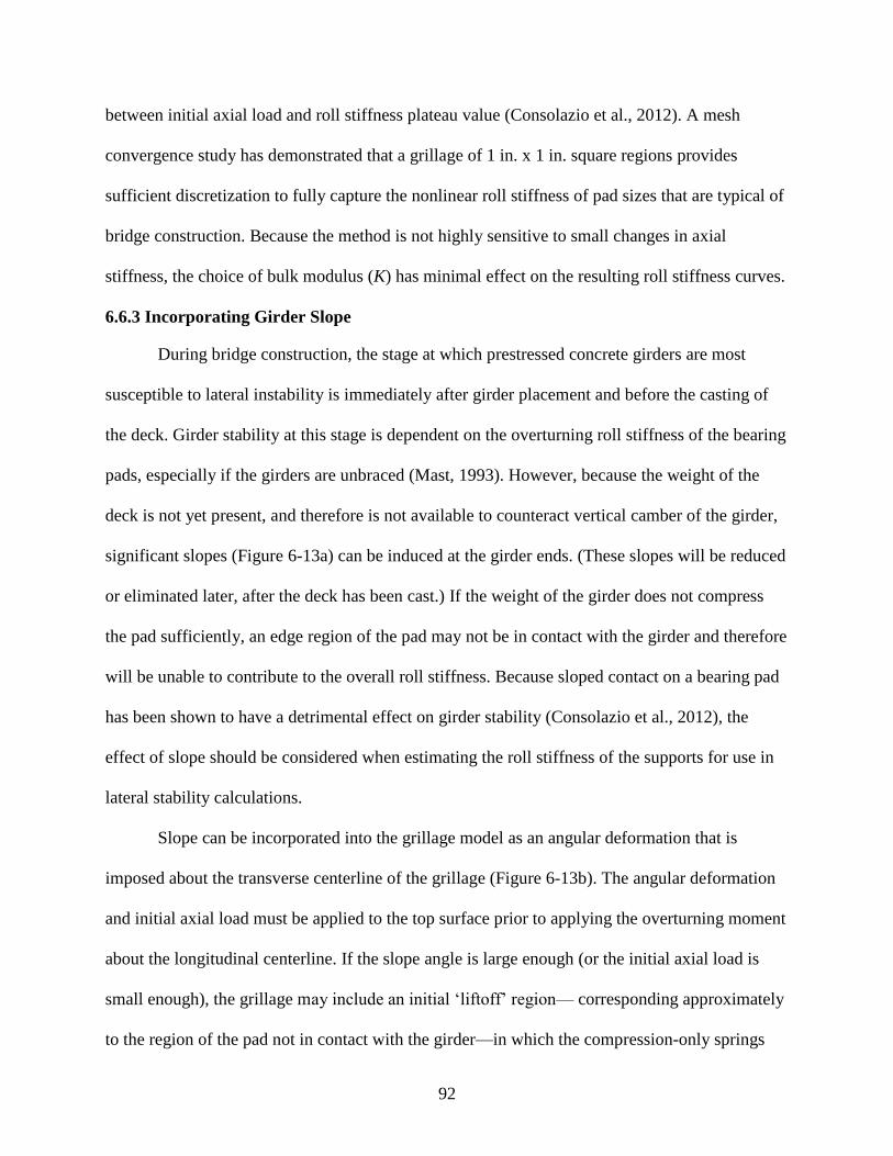
92
between initial axial load and roll stiffness plateau value (Consolazio et al., 2012). A mesh
convergence study has demonstrated that a grillage of 1 in. x 1 in. square regions provides
sufficient discretization to fully capture the nonlinear roll stiffness of pad sizes that are typical of
bridge construction. Because the method is not highly sensitive to small changes in axial
stiffness, the choice of bulk modulus (K) has minimal effect on the resulting roll stiffness curves.
6.6.3 Incorporating Girder Slope
During bridge construction, the stage at which prestressed concrete girders are most
susceptible to lateral instability is immediately after girder placement and before the casting of
the deck. Girder stability at this stage is dependent on the overturning roll stiffness of the bearing
pads, especially if the girders are unbraced (Mast, 1993). However, because the weight of the
deck is not yet present, and therefore is not available to counteract vertical camber of the girder,
significant slopes (Figure 6-13a) can be induced at the girder ends. (These slopes will be reduced
or eliminated later, after the deck has been cast.) If the weight of the girder does not compress
the pad sufficiently, an edge region of the pad may not be in contact with the girder and therefore
will be unable to contribute to the overall roll stiffness. Because sloped contact on a bearing pad
has been shown to have a detrimental effect on girder stability (Consolazio et al., 2012), the
effect of slope should be considered when estimating the roll stiffness of the supports for use in
lateral stability calculations.
Slope can be incorporated into the grillage model as an angular deformation that is
imposed about the transverse centerline of the grillage (Figure 6-13b). The angular deformation
and initial axial load must be applied to the top surface prior to applying the overturning moment
about the longitudinal centerline. If the slope angle is large enough (or the initial axial load is
small enough), the grillage may include an initial ‘liftoff’ region— corresponding approximately
to the region of the pad not in contact with the girder—in which the compression-only springs
93
generate no force. As roll angle increases, the superposition of roll angle and slope angle will
cause the liftoff region to change shape. The resulting roll stiffnesses curves do not match
experimental measurements (Figure 6-14) as closely as in the unsloped cases, however they are
found to be conservatively low. In each case, the initial stiffness predicted by the grillage
approach consistently remains within 40% of the lowest measured stiffness for that case.
6.7 Simplified Method for Calculating Axial Stiffness and Instantaneous Roll Stiffnesses
The calculation methods described in the previous sections produce accurate results, but
require the use of finite element software (to compute kaxial) and structural analysis software (to
compute kroll). For bridge designers, the use of such software may be time consuming and
impractical, particularly if the analyses have to be repeated several times during an iterative
design process. While the grillage method is capable of producing complete nonlinear roll
stiffness curves, some applications require only knowledge of the initial (instantaneous) roll
stiffness. For such cases, it is possible to derive an expression for the initial roll stiffness of the
grillage in closed form, obviating the need to construct and analyze a structural model. This is
accomplished by considering a continuous grillage: a grillage discretized into an infinite number
of springs, each representing an infinitesimal differential area of the pad, dA. Such a grillage can
be treated mathematically as a continuum, and properties (such as roll stiffness) arising from the
aggregated actions of individual springs can be determined in closed-form by integrating over
the area of the pad.
In the sections below, simplified methods for computing axial pad stiffness, kaxial, and
instantaneous pad roll stiffness, kroll, are described.
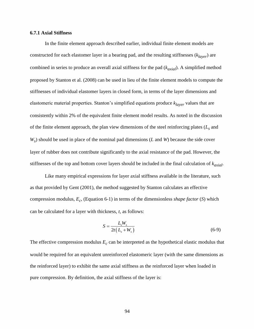
94
6.7.1 Axial Stiffness
In the finite element approach described earlier, individual finite element models are
constructed for each elastomer layer in a bearing pad, and the resulting stiffnesses (klayer) are
combined in series to produce an overall axial stiffness for the pad (kaxial). A simplified method
proposed by Stanton et al. (2008) can be used in lieu of the finite element models to compute the
stiffnesses of individual elastomer layers in closed form, in terms of the layer dimensions and
elastomeric material properties. Stanton’s simplified equations produce klayer values that are
consistently within 2% of the equivalent finite element model results. As noted in the discussion
of the finite element approach, the plan view dimensions of the steel reinforcing plates (Ls and
Ws) should be used in place of the nominal pad dimensions (L and W) because the side cover
layer of rubber does not contribute significantly to the axial resistance of the pad. However, the
stiffnesses of the top and bottom cover layers should be included in the final calculation of kaxial.
Like many empirical expressions for layer axial stiffness available in the literature, such
as that provided by Gent (2001), the method suggested by Stanton calculates an effective
compression modulus, Ec, (Equation 6-1) in terms of the dimensionless shape factor (S) which
can be calculated for a layer with thickness, t, as follows:
2
s s
s s
L WS
t L W
(6-9)
The effective compression modulus Ec can be interpreted as the hypothetical elastic modulus that
would be required for an equivalent unreinforced elastomeric layer (with the same dimensions as
the reinforced layer) to exhibit the same axial stiffness as the reinforced layer when loaded in
pure compression. By definition, the axial stiffness of the layer is:
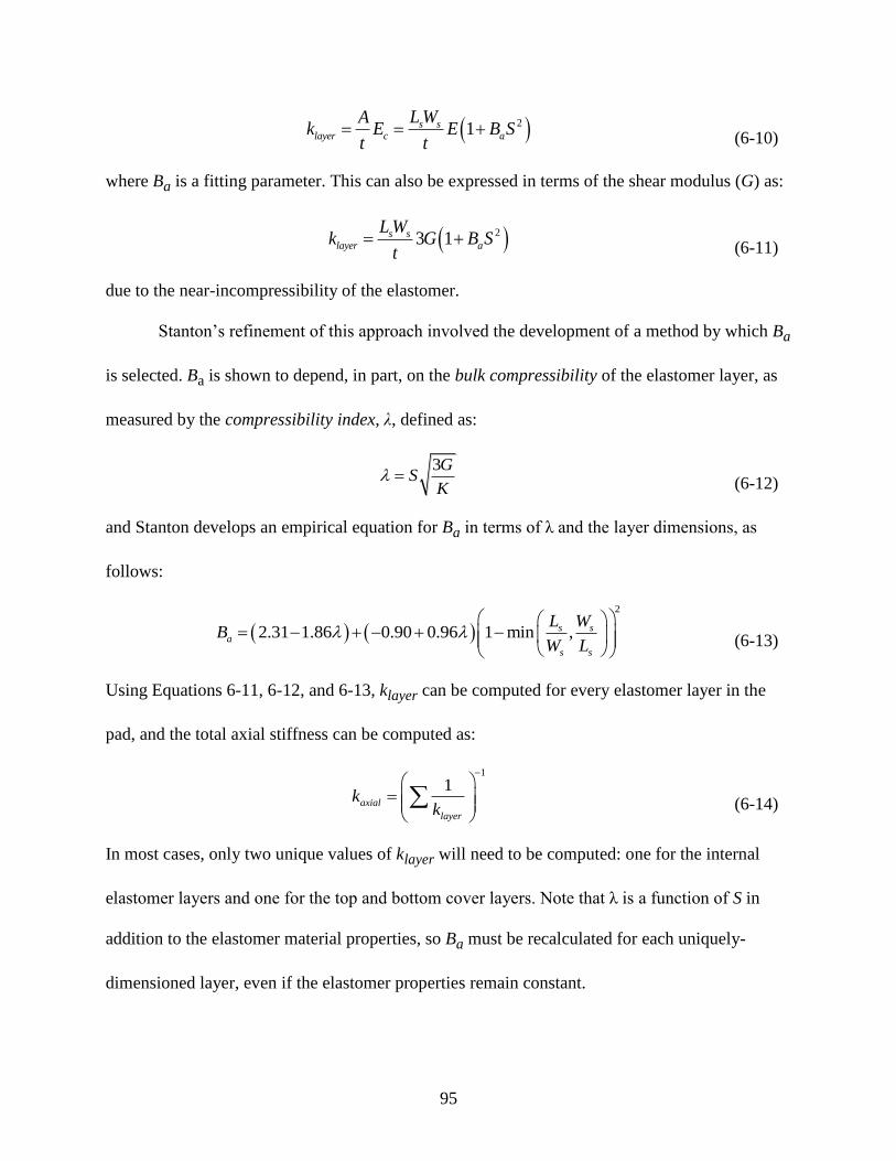
95
21s slayer c a
L WAk E E B S
t t
(6-10)
where Ba is a fitting parameter. This can also be expressed in terms of the shear modulus (G) as:
23 1s slayer a
L Wk G B S
t
(6-11)
due to the near-incompressibility of the elastomer.
Stanton’s refinement of this approach involved the development of a method by which Ba
is selected. Ba is shown to depend, in part, on the bulk compressibility of the elastomer layer, as
measured by the compressibility index, λ, defined as:
3GS
K
(6-12)
and Stanton develops an empirical equation for Ba in terms of λ and the layer dimensions, as
follows:
2
2.31 1.86 0.90 0.96 1 min ,s sa
s s
L WB
W L
(6-13)
Using Equations 6-11, 6-12, and 6-13, klayer can be computed for every elastomer layer in the
pad, and the total axial stiffness can be computed as:
1
1axial
layer
kk
(6-14)
In most cases, only two unique values of klayer will need to be computed: one for the internal
elastomer layers and one for the top and bottom cover layers. Note that λ is a function of S in
addition to the elastomer material properties, so Ba must be recalculated for each uniquely-
dimensioned layer, even if the elastomer properties remain constant.
96
6.7.2 Basic Derivation of Instantaneous Roll Stiffness of a Continuous Grillage
The following derivations employ a principal coordinate system (x,y) in which roll occurs
about the y-axis. In these coordinates, the pad (and, therefore, the grillage) extends ±0.5W in the
x-direction and ±0.5L in the y-direction (Figure 6-15). Stiffness of roll about the x-axis can be
obtained by transposing the values of W and L.
Instantaneous roll stiffness of a continuous grillage is determined by imposing a
differential angular displacement in the direction of roll (dθ) and computing the total restoring
moment (dM) generated by the resulting spring forces. Recall from Figure 6-11 that the stiffness
of each spring varies depending on its location within the grillage according to a scaled bubble
function expressed in normalized coordinates. In principal coordinates, the stiffness at every
point (x,y), is:
2 2
, 1 10.5 0.5
axialspring
pad
k x yk x y dA
A W L
(6-15)
When a differential roll angle (dθ) is imposed about the y-axis, an axial displacement field is
produced, so that every spring displaces a vertical distance of:
,z x y xd (6-16)
depending on its distance from the roll axis. At every point (x,y), the total axial restoring force is
therefore the product of kspring(x,y) and Δz(x,y). Because each spring has a moment arm of x (the
distance from the y-axis), the total restoring moment exerted by the deformed grillage of springs
can be computed with the following integral:
, ,spring
A
dM x z x y k x y (6-17)
97
Substituting Equations 6-15 and 6-16 into Equation 6-17, rewriting Apad as the product
LW, and dividing through by dθ results in an integral expression for the instantaneous roll
stiffness of the grillage:
2 2
2 1 10.5 0.5
axialroll
A
kdM x yk x dA
d LW W L
(6-18)
in terms of L, W, kaxial, and the coordinate variables x and y. To evaluate the surface integral in
closed-form, it is necessary to reformulate it as a double integral in x and y, evaluated over the
plan-view dimensions of the pad:
2 20.5 0.5
2
0.5 0.51 1
0.5 0.5
L Waxial
rollL W
k x yk x dxdy
LW W L
(6-19)
which reduces to a simple closed-form expression:
2
45
axialroll
k Wk
(6-20)
in terms of only the total axial stiffness of the pad (kaxial) and the width of the pad in the
direction perpendicular to the roll axis (W).
6.7.3 Incorporating Girder Slope
By integrating over the entire plan-view area of the bearing pad (i.e., the grillage), the
preceding derivation assumes that the entire surface of the pad is in contact with the girder. This
assumption may not hold if there is a non-zero slope angle (ϕ), as the total axial load exerted on
the pad by the girder may not be sufficient to compress the pad far enough to achieve full contact
(recall Figure 6-13). Such a condition reduces the effective area of the pad that contributes to roll
stiffness. This phenomenon can be accounted for in the calculation by altering the limits of
integration to include only the region of the bearing pad grillage that is in initial contact with the
girder, as follows:
98
2 20.5 0.5
2
0.5 0.51 1
0.5 0.5
L pL Waxial
rollL W
k x yk x dxdy
LW W L
(6-21)
where p is the proportion of the pad area that is in contact (0 ≤ p ≤ 1). Closed-form evaluation of
the modified integral produces the expression:
2
2 3 245
axialroll
k Wk p p
(6-22)
which reduces to Equation 6-20 when p = 1.
For a given configuration, the value of p depends on the total distance that the grillage is
initially compressed, which is a function of both ϕ and the initial axial load resulting from girder
self-weight (Faxial). When Faxial is applied, the sloped upper surface of the grillage deforms
downward (increasing the contact area) until the total restoring force in the compressed springs
achieves equilibrium with Faxial. From statics, the force equilibrium equation for the continuous
grillage is:
, ,axial spring
A
F z x y k x y dA (6-23)
where Δz(x,y) is the displacement field imposed on the bearing pad grillage by the sloped surface
of the girder. Slope-induced displacements, Δz(x,y), do not vary in the x-direction, and can
therefore be expressed as a line in the y-z plane, with slope ϕ and y-intercept p, as follows:
, 0.5z x y y L pL (6-24)
where (−0.5L + pL) is the y-coordinate of p in principal coordinates. Substituting Equations 6-24
and 6-15 into Equation 6-23 and reformulating it as a double integral (which must also include p
in the limits of integration), results in the following equation:
2 2
0.5 0.5
0.5 0.50.5 1 1
0.5 0.5
L pL Waxial
axialL W
k x yF y L pL dxdy
LW W L
(6-25)
99
322
9axial axialF L k p p
(6-26)
in which p is the only unknown. Rearranging the terms of Equation 6-26 yields:
4 3 92 0 where
2
axial
axial
Fp p
L k
(6-27)
revealing p to be the root of a quartic equation.
For polynomials of degree < 5, general solutions for the roots can be expressed as closed-
form equations in terms of the polynomial coefficients. In the case of Equation 6-27, there are
four roots and four corresponding equations (omitted here for brevity). Recall that the quantity p
is only meaningful over the interval 0 ≤ p ≤ 1, and note that if p = 0, η must also be 0; if p = 1, η
must also be 1; and within that interval, η increases monotonically with p. Consequently,
solutions for p need only be defined over the interval, 0 ≤ η ≤ 1. Upon substituting the
polynomial coefficients from Equation 6-27 (quartic in p: 1; cubic in p: −2; quadratic in p:
0; linear in p: 0; and constant: η) into the four root equations, the only one that results in a
positive real root within the intended range for 0 ≤ η ≤ 1 reduces to:
2 4
2 3
3
1 3 4
2 2
1where B and
2 6 4 4 4 3
B B Bp B
B
AA
A
(6-28)
Equation 6-28, which is exact but somewhat cumbersome, can be closely and
conservatively approximated as the much simpler (Figure 6-17). In practice, given the
empirical approximations introduced by the grillage representation of a bearing pad and the
inherent variability in pad construction and behavior, the error introduced by using in place
of Equation 6-28 is insignificant. Substituting in the definition of η from Equation 6-27, the final
expression for the approximate instantaneous roll stiffness of a rectangular bearing pad is:

100
2
2
1.0 if 0
3 2 where 91.0 if 045
2
axialroll axial
axial
k Wk p p p F
L k
(6-29)
where kaxial is the total axial stiffness of the pad, Faxial is the initial axial load (i.e., the reaction
on the pad due to girder weight), ϕ is the girder slope angle, and L and W are the plan-view
dimensions of the pad (perpendicular to and parallel to the roll axis, respectively).
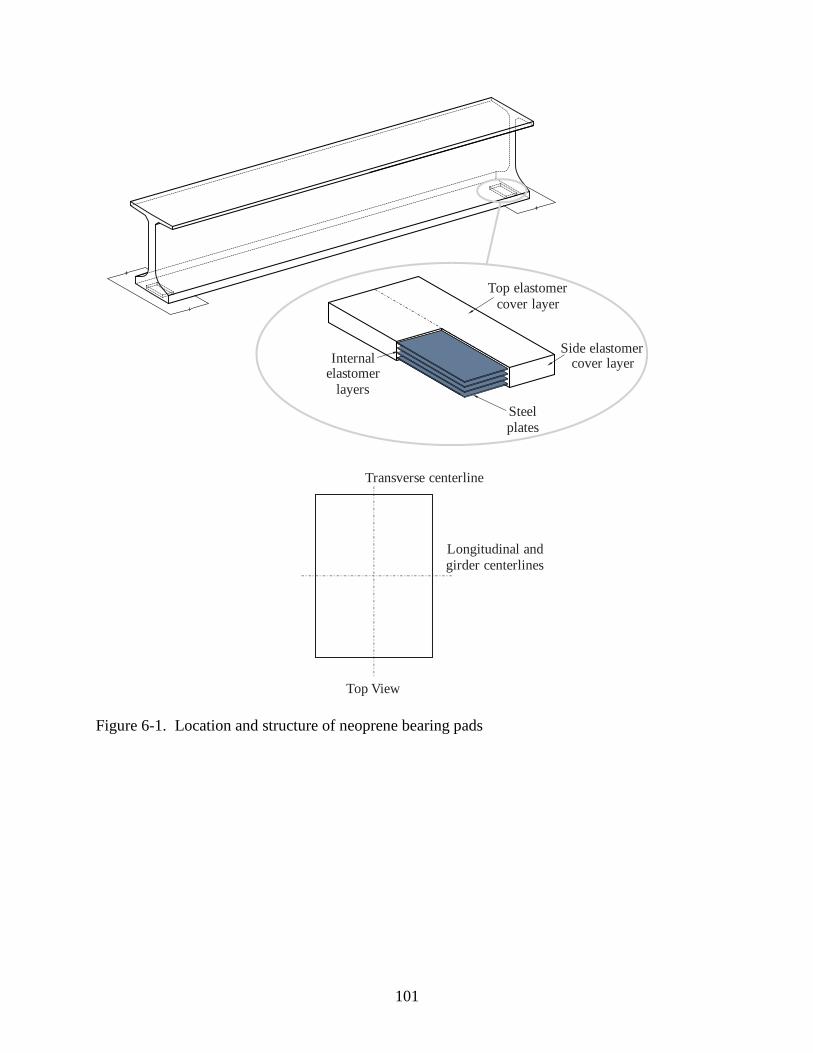
101
Top elastomer
cover layer
Steel
plates
Internal elastomer
layers
Side elastomer cover layer
Longitudinal and
girder centerlines
Transverse centerline
Top View
Figure 6-1. Location and structure of neoprene bearing pads
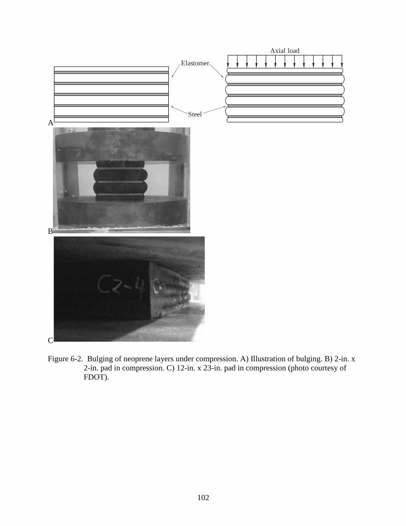
102
A
Axial load
Steel
Elastomer
B
C
Figure 6-2. Bulging of neoprene layers under compression. A) Illustration of bulging. B) 2-in. x
2-in. pad in compression. C) 12-in. x 23-in. pad in compression (photo courtesy of
FDOT).
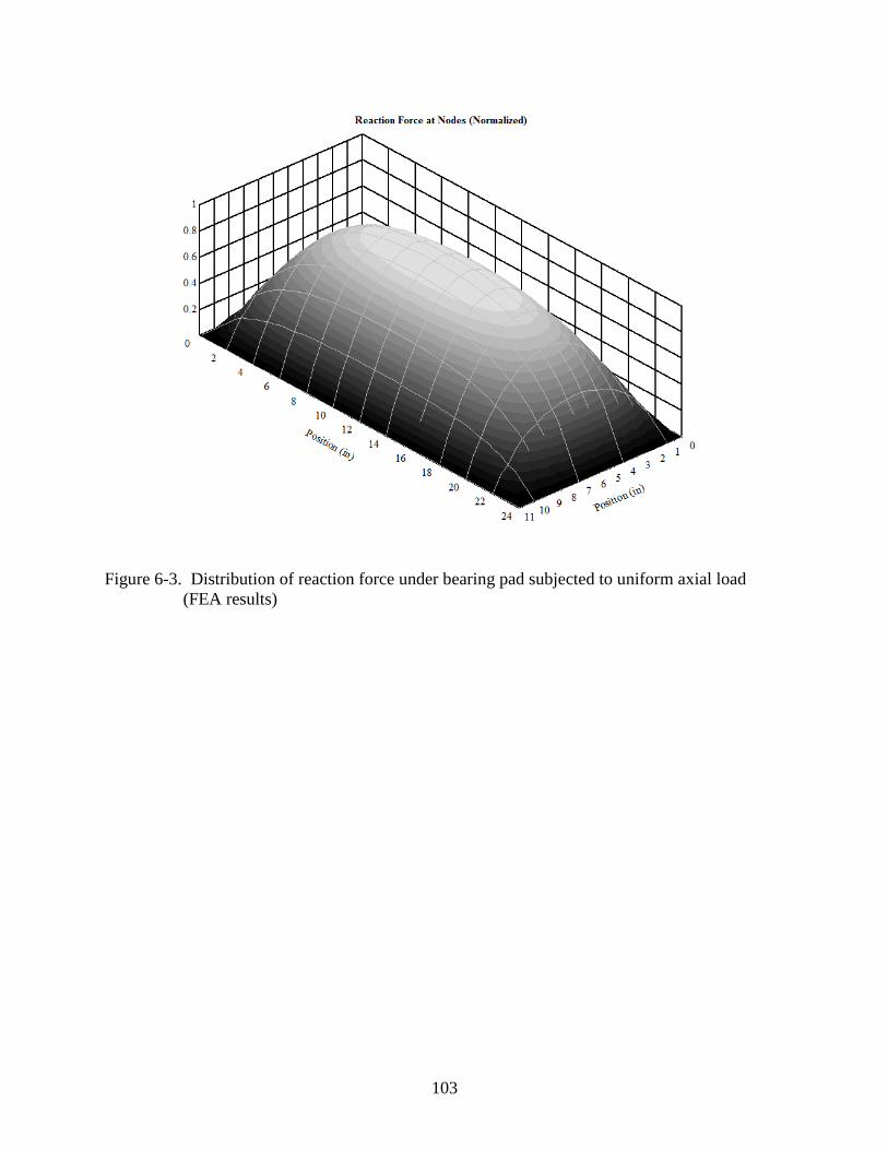
103
Figure 6-3. Distribution of reaction force under bearing pad subjected to uniform axial load
(FEA results)
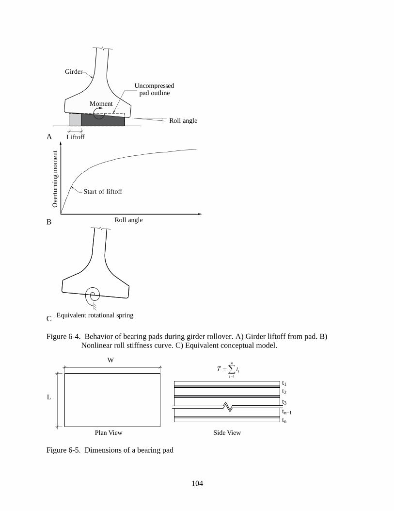
104
A
Roll angle
Girder
Liftoff
Uncompressed pad outline
Moment
B Roll angle
Over
turn
ing
mo
me
nt
Start of liftoff
CEquivalent rotational spring
Figure 6-4. Behavior of bearing pads during girder rollover. A) Girder liftoff from pad. B)
Nonlinear roll stiffness curve. C) Equivalent conceptual model.
t1t2
t3
tn−1
tn
Side ViewPlan View
W
L
Figure 6-5. Dimensions of a bearing pad
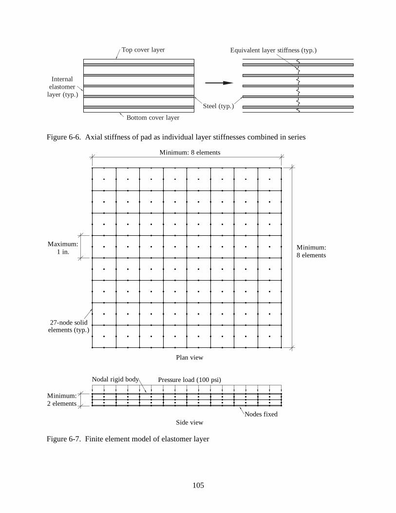
105
Top cover layer
Bottom cover layer
Internal
elastomer
layer (typ.)
Steel (typ.)
Equivalent layer stiffness (typ.)
Figure 6-6. Axial stiffness of pad as individual layer stiffnesses combined in series
Minimum: 8 elements
Minimum:
8 elements
Maximum:
1 in.
Minimum:
2 elements
Pressure load (100 psi)
27-node solid elements (typ.)
Nodal rigid body
Nodes fixed
Plan view
Side view
Figure 6-7. Finite element model of elastomer layer
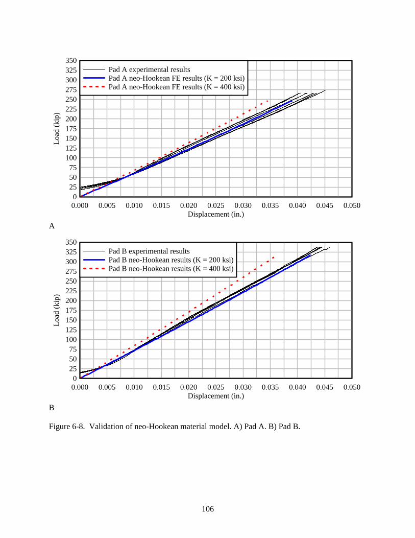
106
A
B
Figure 6-8. Validation of neo-Hookean material model. A) Pad A. B) Pad B.
Displacement (in.)
Lo
ad (
kip
)
0.000 0.005 0.010 0.015 0.020 0.025 0.030 0.035 0.040 0.045 0.050
0
25
50
75
100
125
150
175
200
225
250
275
300
325
350
Pad A experimental results
Pad A neo-Hookean FE results (K = 200 ksi)
Pad A neo-Hookean FE results (K = 400 ksi)
Displacement (in.)
Lo
ad (
kip
)
0.000 0.005 0.010 0.015 0.020 0.025 0.030 0.035 0.040 0.045 0.050
0
25
50
75
100
125
150
175
200
225
250
275
300
325
350
Pad B experimental results
Pad B neo-Hookean results (K = 200 ksi)
Pad B neo-Hookean results (K = 400 ksi)
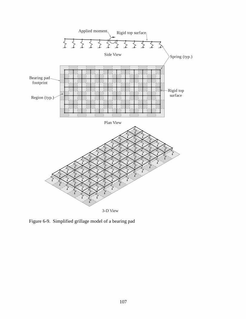
107
Side View
Plan View
Bearing pad
footprint
Region (typ.)
Spring (typ.)
Rigid top surfaceApplied moment
Rigid top
surface
3-D View
Figure 6-9. Simplified grillage model of a bearing pad

108
10 gage steel
plates (typ.)
H
0.25 in. elastomer
cover (typ.)
0.5 in. internal
elastomer layer (typ.)H
L or W
W
L or W
0.25 in. elastomer
cover layer (typ.)
L
Typical section: Bearing pad types B & C
Plan view
Bearing pad types A, B & C
Typical section: Bearing pad type A
Bearing pad type
A B C
Bearing pad length, L (in.) 11 14 12
Bearing pad width, W (in.) 24 24 23
Bearing pad height, H (in.) 1-29/32 2-9/16 2-9/16
Number of internal plates 3 4 4
Figure 6-10. Standard FDOT bearing pads used for experimental verification
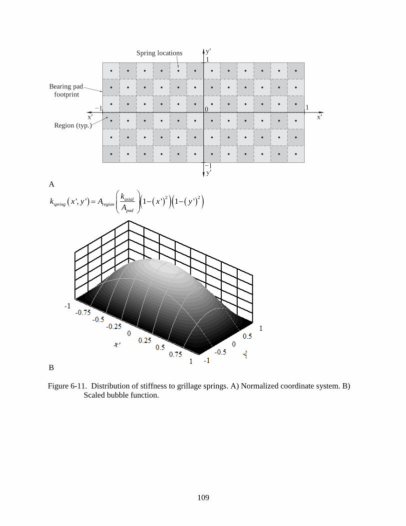
109
Bearing pad
footprint
Region (typ.)
y′
0
1
1−1
−1
x′x′
y′Spring locations
A
2 2', ' 1 ' 1 'axial
spring region
pad
kk x y A x y
A
B
Figure 6-11. Distribution of stiffness to grillage springs. A) Normalized coordinate system. B)
Scaled bubble function.
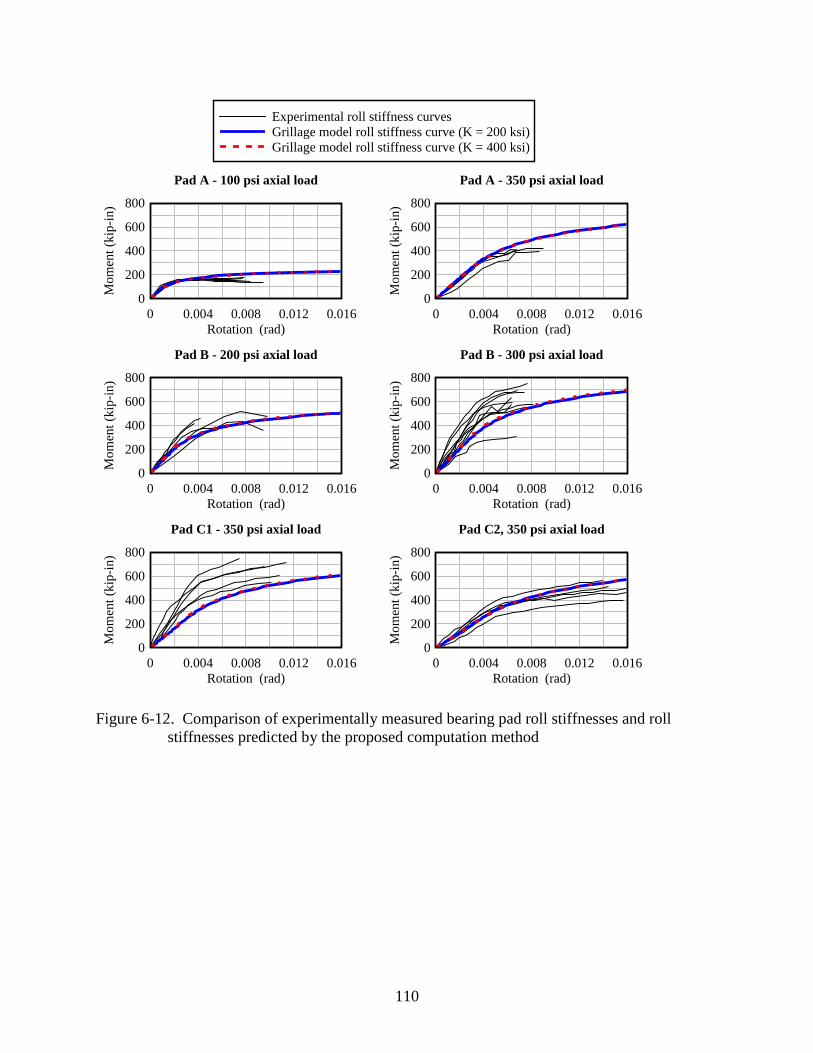
110
Figure 6-12. Comparison of experimentally measured bearing pad roll stiffnesses and roll
stiffnesses predicted by the proposed computation method
Experimental roll stiffness curves
Grillage model roll stiffness curve (K = 200 ksi)
Grillage model roll stiffness curve (K = 400 ksi)
Rotation (rad)
Mom
ent
(kip
-in)
Pad A - 100 psi axial load
0 0.004 0.008 0.012 0.016
0
200
400
600
800
Rotation (rad)
Mom
ent
(kip
-in)
Pad A - 350 psi axial load
0 0.004 0.008 0.012 0.016
0
200
400
600
800
Rotation (rad)
Mom
ent
(kip
-in)
Pad B �- 200 psi axial load
0 0.004 0.008 0.012 0.016
0
200
400
600
800
Rotation (rad)
Mom
ent
(kip
-in)
Pad B - 300 psi axial load
0 0.004 0.008 0.012 0.016
0
200
400
600
800
Rotation (rad)
Mom
ent
(kip
-in)
Pad C1 - 350 psi axial load
0 0.004 0.008 0.012 0.016
0
200
400
600
800
Rotation (rad)
Mom
ent
(kip
-in)
Pad C2, 350 psi axial load
0 0.004 0.008 0.012 0.016
0
200
400
600
800
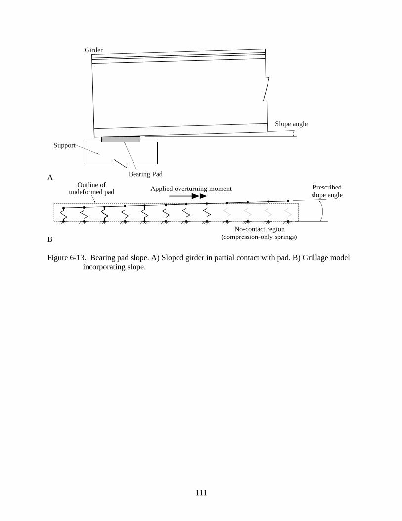
111
A Bearing Pad
Support
Girder
Slope angle
B
Prescribed
slope angleApplied overturning moment
Outline of u ndeformed pad
No-contact region
(compression-only springs)
Figure 6-13. Bearing pad slope. A) Sloped girder in partial contact with pad. B) Grillage model
incorporating slope.
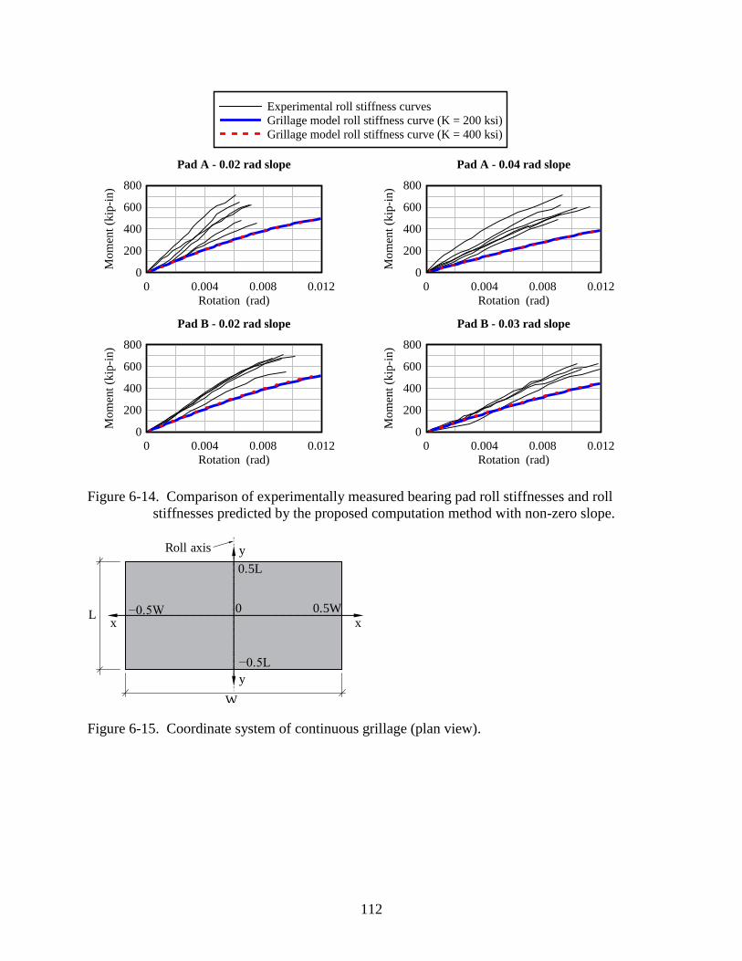
112
Figure 6-14. Comparison of experimentally measured bearing pad roll stiffnesses and roll
stiffnesses predicted by the proposed computation method with non-zero slope.
y
0
xx
y
W
L
0.5L
−0.5L
0.5W−0.5W
Roll axis
Figure 6-15. Coordinate system of continuous grillage (plan view).
Experimental roll stiffness curves
Grillage model roll stiffness curve (K = 200 ksi)
Grillage model roll stiffness curve (K = 400 ksi)
Rotation (rad)
Mom
ent
(kip
-in)
Pad A - 0.02 rad slope
0 0.004 0.008 0.012
0
200
400
600
800
Rotation (rad)
Mom
ent
(kip
-in)
Pad A - 0.04 rad slope
0 0.004 0.008 0.012
0
200
400
600
800
Rotation (rad)
Mom
ent
(kip
-in)
Pad B - 0.02 rad slope
0 0.004 0.008 0.012
0
200
400
600
800
Rotation (rad)
Mom
ent
(kip
-in)
Pad B - 0.03 rad slope
0 0.004 0.008 0.012
0
200
400
600
800
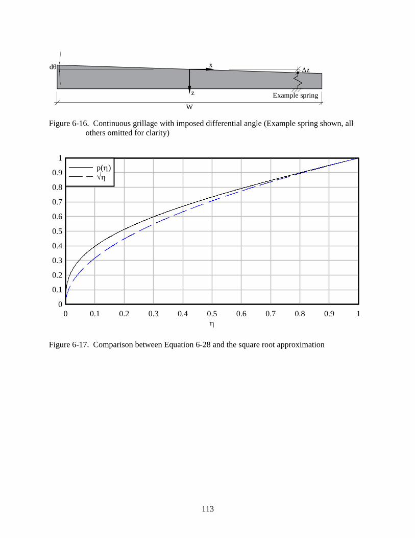
113
z
xΔzdθ
W
Example spring
Figure 6-16. Continuous grillage with imposed differential angle (Example spring shown, all
others omitted for clarity)
Figure 6-17. Comparison between Equation 6-28 and the square root approximation
0 0.1 0.2 0.3 0.4 0.5 0.6 0.7 0.8 0.9 1
0
0.1
0.2
0.3
0.4
0.5
0.6
0.7
0.8
0.9
1
p()
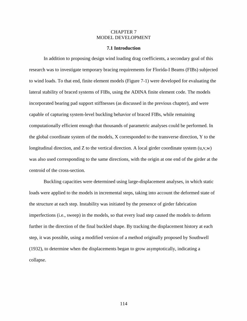
114
CHAPTER 7
MODEL DEVELOPMENT
7.1 Introduction
In addition to proposing design wind loading drag coefficients, a secondary goal of this
research was to investigate temporary bracing requirements for Florida-I Beams (FIBs) subjected
to wind loads. To that end, finite element models (Figure 7-1) were developed for evaluating the
lateral stability of braced systems of FIBs, using the ADINA finite element code. The models
incorporated bearing pad support stiffnesses (as discussed in the previous chapter), and were
capable of capturing system-level buckling behavior of braced FIBs, while remaining
computationally efficient enough that thousands of parametric analyses could be performed. In
the global coordinate system of the models, X corresponded to the transverse direction, Y to the
longitudinal direction, and Z to the vertical direction. A local girder coordinate system (u,v,w)
was also used corresponding to the same directions, with the origin at one end of the girder at the
centroid of the cross-section.
Buckling capacities were determined using large-displacement analyses, in which static
loads were applied to the models in incremental steps, taking into account the deformed state of
the structure at each step. Instability was initiated by the presence of girder fabrication
imperfections (i.e., sweep) in the models, so that every load step caused the models to deform
further in the direction of the final buckled shape. By tracking the displacement history at each
step, it was possible, using a modified version of a method originally proposed by Southwell
(1932), to determine when the displacements began to grow asymptotically, indicating a
collapse.
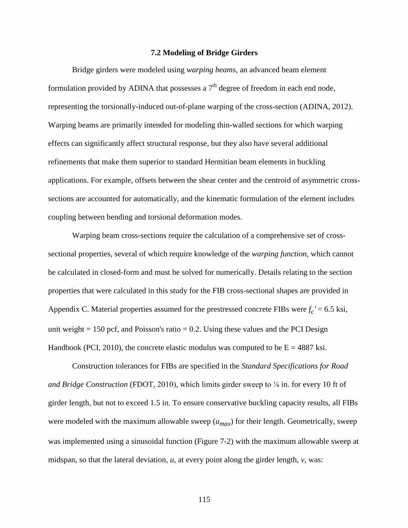
115
7.2 Modeling of Bridge Girders
Bridge girders were modeled using warping beams, an advanced beam element
formulation provided by ADINA that possesses a 7th
degree of freedom in each end node,
representing the torsionally-induced out-of-plane warping of the cross-section (ADINA, 2012).
Warping beams are primarily intended for modeling thin-walled sections for which warping
effects can significantly affect structural response, but they also have several additional
refinements that make them superior to standard Hermitian beam elements in buckling
applications. For example, offsets between the shear center and the centroid of asymmetric cross-
sections are accounted for automatically, and the kinematic formulation of the element includes
coupling between bending and torsional deformation modes.
Warping beam cross-sections require the calculation of a comprehensive set of cross-
sectional properties, several of which require knowledge of the warping function, which cannot
be calculated in closed-form and must be solved for numerically. Details relating to the section
properties that were calculated in this study for the FIB cross-sectional shapes are provided in
Appendix C. Material properties assumed for the prestressed concrete FIBs were fc′ = 6.5 ksi,
unit weight = 150 pcf, and Poisson's ratio = 0.2. Using these values and the PCI Design
Handbook (PCI, 2010), the concrete elastic modulus was computed to be E = 4887 ksi.
Construction tolerances for FIBs are specified in the Standard Specifications for Road
and Bridge Construction (FDOT, 2010), which limits girder sweep to ⅛ in. for every 10 ft of
girder length, but not to exceed 1.5 in. To ensure conservative buckling capacity results, all FIBs
were modeled with the maximum allowable sweep (umax) for their length. Geometrically, sweep
was implemented using a sinusoidal function (Figure 7-2) with the maximum allowable sweep at
midspan, so that the lateral deviation, u, at every point along the girder length, v, was:
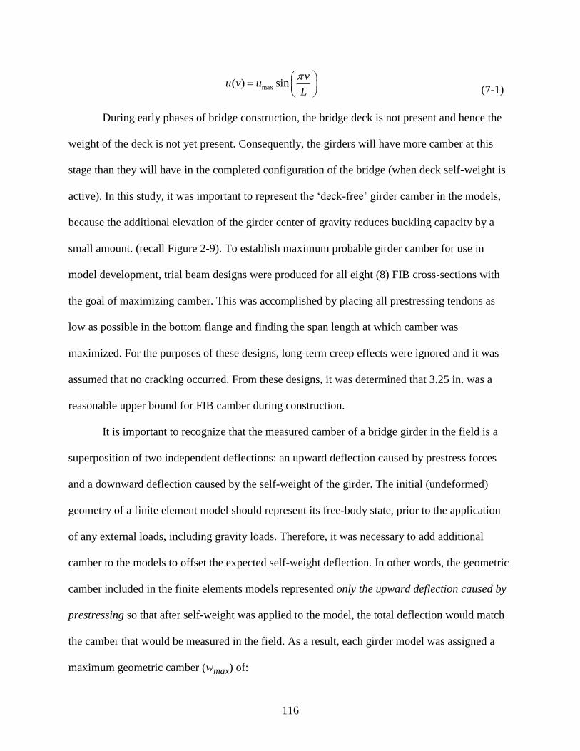
116
max( ) sinv
u v uL
(7-1)
During early phases of bridge construction, the bridge deck is not present and hence the
weight of the deck is not yet present. Consequently, the girders will have more camber at this
stage than they will have in the completed configuration of the bridge (when deck self-weight is
active). In this study, it was important to represent the ‘deck-free’ girder camber in the models,
because the additional elevation of the girder center of gravity reduces buckling capacity by a
small amount. (recall Figure 2-9). To establish maximum probable girder camber for use in
model development, trial beam designs were produced for all eight (8) FIB cross-sections with
the goal of maximizing camber. This was accomplished by placing all prestressing tendons as
low as possible in the bottom flange and finding the span length at which camber was
maximized. For the purposes of these designs, long-term creep effects were ignored and it was
assumed that no cracking occurred. From these designs, it was determined that 3.25 in. was a
reasonable upper bound for FIB camber during construction.
It is important to recognize that the measured camber of a bridge girder in the field is a
superposition of two independent deflections: an upward deflection caused by prestress forces
and a downward deflection caused by the self-weight of the girder. The initial (undeformed)
geometry of a finite element model should represent its free-body state, prior to the application
of any external loads, including gravity loads. Therefore, it was necessary to add additional
camber to the models to offset the expected self-weight deflection. In other words, the geometric
camber included in the finite elements models represented only the upward deflection caused by
prestressing so that after self-weight was applied to the model, the total deflection would match
the camber that would be measured in the field. As a result, each girder model was assigned a
maximum geometric camber (wmax) of:
117
4
max
53.25 in.
384
A Lw
EI
(7-2)
where A is the girder cross-sectional area, γ is the unit weight of the concrete, L is the span
length, E is the elastic modulus, and I is the major-axis moment of inertia.
Because the geometric camber in the models represented upward deflections caused by
straight prestressing tendons (which generate a constant internal moment throughout the length
of the beam), the girder camber was implemented with a parabolic shape (Figure 7-3) so that the
vertical deviation, w, at every point along the girder length, v, was:
2
max( ) 4v v
w v wL L
(7-3)
7.3 Modeling of End Supports
Girder support stiffnesses were modeled with six (6) geometrically linear springs to
represent the stiffness of the bearing pad in each degree of freedom, with each spring
corresponding to one of the four (4) main deformation modes of the pad: shear, axial, torsion,
and roll (Figure 7-4). These stiffnesses were obtained using the calculation methods discussed in
Chapter 6. The roll stiffness springs (in both the overturning and bending directions) were
assigned nonlinear moment-rotation curves that captured the softening effects of partial girder
liftoff from the pad. The remaining pad stiffnesses were treated as linear.
7.3.1 Pad Selection
Seven (7) standard types of elastomeric bearing pad are provided in Design Standard No.
20510: Composite Elastome ric Bearing Pads – Prestressed Florida-I Beams (FDOT, 2012c) for
use with FIBs. During design, selection of the type of pad that will be used in a particular bridge
is based on thermal expansion and live load deflection limit states of the completed bridge,
neither of which can be predicted based solely on girder dimensions (cross-sectional and span
118
length). As such, it is not appropriate to assume that for each FIB type, there is a specific
corresponding type of bearing pad that would be utilized. Hence, in this study, it was
conservatively assumed that the pad type with the lowest roll stiffness (which will produce the
lowest buckling capacity) would be used in conjunction with all FIB types. After calculating the
roll stiffness of every standard FDOT FIB pad type (see Appendix D for details), using the
grillage method that was discussed in Chapter 6, the Type J bearing pad was selected for use in
this study.
7.3.2 Axial Load Selection
In Chapter 6, it was noted that the amount of axial load applied to a pad does not change
the initial linear portion of the roll stiffness curve, but it does affect the moment required to
initiate girder roll-off from the pad. Reducing the compressive axial load on a pad reduces the
moment that is required to cause girder roll-off. Additionally, reducing girder span length
reduces girder self-weight which, in turn, reduces the axial loads on the bearing pads. Therefore,
to be conservative in this study, the minimum length ranges for each FIB shape were determined
from design aids in Instructions for Design Standard No. 20010: Prestressed Florida-I Beams
(IDS 20010; FDOT, 2012b) and the minimum expected axial pad load was calculated for each
FIB shape. (These calculations assumed that the girders were simply supported. Additionally, the
effects of wind uplift forces were conservatively ignored.) Using this process, a single worst-case
(minimized) roll stiffness curve was calculated for each type of FIB, resulting in a total of seven
(7) bearing pad moment-rotation curves.
7.3.3 Girder Slope Selection
In Chapter 6, it was also noted that overturning roll stiffness is reduced by the presence of
girder slope, which can arise from a combination of girder camber and bridge grade. According
to Instructions for Design Standard No. 20510: Composite Elastomeric Bearing Pads –
119
Prestressed Florida-I Beams (IDS 20510; FDOT, 2012d), the maximum expected slope angle in
the completed bridge is 0.0125 rad, because if this angle is exceeded, beveled bearing plates
must be installed to eliminate slope. Therefore, the maximum expected camber prior to the
casting of the deck is the sum of 0.0125 rad and any camber-induced slope that is negated by the
downward deflection under the weight of the deck and other superimposed dead loads (SDL).
After a series of trial beam design calculations was performed, it was determined that a
reasonable upper limit for the SDL-negated slope was 0.01 rad. Additionally, AASHTO LRFD
(2010) recommends an “allowance for uncertainties” of 0.005 rad with regard to bearing pad
slope angle. The maximum completed slope of 0.0125 rad, the SDL-negated slope of 0.01 rad,
and the slope uncertainty of 0.005 rad combined for a total maximum slope angle of 0.0275 rad.
This was conservatively rounded up to a slope angle of 0.03 rad, which was used to compute the
bearing pad overturning roll stiffness curves.
7.4 Modeling of Braces and Anchors
Because the design of bracing has historically been left to the discretion of the contractor,
a wide variety of bracing configurations are used in practice. Consequently, in this study, it was
not possible for every potential brace configuration to be represented in the parametric studies.
After conducting a survey of bracing designs used in the construction of bridges throughout
Florida, four (4) representative brace configurations were identified:
Top strut (Figure 7-5a): a horizontal timber compression strut situated between the
edges of the top flanges. The top strut is typically nailed to the underside of a slightly
longer timber member, creating ‘lips’ that rest on the top of the flanges.
Parallel strut (Figure 7-5b): Two (or more) horizontal timber compression struts
wedged in place between the girder webs.
X-brace (Figure 7-5c): Two diagonal timber members wedged between the webs that
cross in the middle to form an ‘X’ shape. A steel bolt typically passes through both
members at the crossing point to create a hinge.
120
K-brace (Figure 7-5d): Steel members (typically steel angles) welded together into a
‘K’-shaped frame and welded or bolted to steel plates cast into the webs.
The majority of brace designs that were encountered were variations of one of these four basic
configurations.
For analysis purposes, braces were modeled primarily with beam elements, with each
brace member represented by a single element. At the girder connection points, rigid links were
used to connect the braces to the girder elements (i.e., warping beams located at the girder
centroids). It was assumed that the brace–girder connections were ideal pins, which was
conservative with regard to girder stability. Pins and hinges were modeled with beam end-
releases and nodal constraints, respectively.
During the survey of bracing designs, the vast majority of timber braces that were
encountered were composed of 4x4 Southern Pine sawn lumber. According to the National
Design Specification for Wood Construction (AF&PA, 2005), 4x4 Southern Pine has a
3.5″ x 3.5″ square cross-section and an elastic modulus of E = 495 ksi (based on an Emin of
550 ksi for 4-inch-wide “Construction-grade” lumber and a Wet Service Factor of 0.9). These
properties were used to model all timber brace members including the top strut, parallel strut,
and X-brace. Based on a typical bridge bracing design that was acquired during the survey,
K-brace members were modeled as 4″ x 4″ x ⅜″ steel angles, with an elastic modulus of E =
29000 ksi.
In contrast to braces, girder anchors were not modeled with structural elements. Instead,
the additional roll stiffness provided by the anchors (kroll,anchor) was quantified directly and
added to the bearing pad support stiffness (kroll,overturning). It was assumed that only one FIB in
each bridge cross-section was anchored and that anchors at each end of the girder were of equal
stiffness.
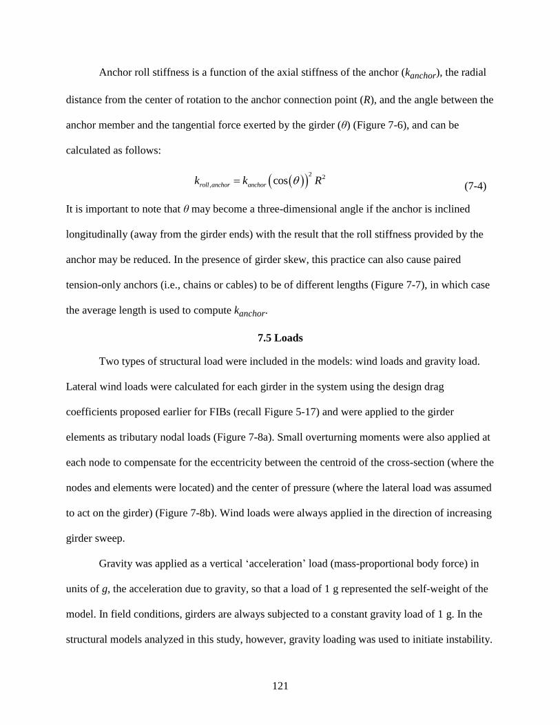
121
Anchor roll stiffness is a function of the axial stiffness of the anchor (kanchor), the radial
distance from the center of rotation to the anchor connection point (R), and the angle between the
anchor member and the tangential force exerted by the girder (θ) (Figure 7-6), and can be
calculated as follows:
2 2
, cosroll anchor anchork k R (7-4)
It is important to note that θ may become a three-dimensional angle if the anchor is inclined
longitudinally (away from the girder ends) with the result that the roll stiffness provided by the
anchor may be reduced. In the presence of girder skew, this practice can also cause paired
tension-only anchors (i.e., chains or cables) to be of different lengths (Figure 7-7), in which case
the average length is used to compute kanchor.
7.5 Loads
Two types of structural load were included in the models: wind loads and gravity load.
Lateral wind loads were calculated for each girder in the system using the design drag
coefficients proposed earlier for FIBs (recall Figure 5-17) and were applied to the girder
elements as tributary nodal loads (Figure 7-8a). Small overturning moments were also applied at
each node to compensate for the eccentricity between the centroid of the cross-section (where the
nodes and elements were located) and the center of pressure (where the lateral load was assumed
to act on the girder) (Figure 7-8b). Wind loads were always applied in the direction of increasing
girder sweep.
Gravity was applied as a vertical ‘acceleration’ load (mass-proportional body force) in
units of g, the acceleration due to gravity, so that a load of 1 g represented the self-weight of the
model. In field conditions, girders are always subjected to a constant gravity load of 1 g. In the
structural models analyzed in this study, however, gravity loading was used to initiate instability.
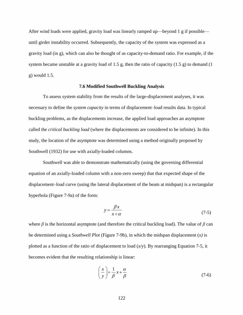
122
After wind loads were applied, gravity load was linearly ramped up—beyond 1 g if possible—
until girder instability occurred. Subsequently, the capacity of the system was expressed as a
gravity load (in g), which can also be thought of as capacity-to-demand ratio. For example, if the
system became unstable at a gravity load of 1.5 g, then the ratio of capacity (1.5 g) to demand (1
g) would 1.5.
7.6 Modified Southwell Buckling Analysis
To assess system stability from the results of the large-displacement analyses, it was
necessary to define the system capacity in terms of displacement–load results data. In typical
buckling problems, as the displacements increase, the applied load approaches an asymptote
called the critical buckling load (where the displacements are considered to be infinite). In this
study, the location of the asymptote was determined using a method originally proposed by
Southwell (1932) for use with axially-loaded columns.
Southwell was able to demonstrate mathematically (using the governing differential
equation of an axially-loaded column with a non-zero sweep) that that expected shape of the
displacement–load curve (using the lateral displacement of the beam at midspan) is a rectangular
hyperbola (Figure 7-9a) of the form:
xy
x
(7-5)
where β is the horizontal asymptote (and therefore the critical buckling load). The value of β can
be determined using a Southwell Plot (Figure 7-9b), in which the midspan displacement (x) is
plotted as a function of the ratio of displacement to load (x/y). By rearranging Equation 7-5, it
becomes evident that the resulting relationship is linear:
1xx
y
(7-6)

123
with the critical buckling load being equal to the inverse slope of the line (Figure 7-9b). The
critical buckling load can therefore be determined by applying linear least-squares regression to
the transformed analysis results (i.e., pairs of x and x/y values). Using this technique, reliable
determination of the critical load can be obtained from displacement–load data, even if only a
portion of the overall displacement–load plot is available. (This aspect of the method is
particularly useful for physical testing, as specimens do not need to be loaded all the way to
failure in order for the buckling capacity to be quantified.)
Theoretically, the mathematical foundation for the Southwell method is only valid for
axial column buckling. For this reason, several authors (Massey, 1963; Trahair, 1969; Meck,
1977) have published alternative methods mathematically formulated for lateral stability
problems (based on the governing differential equation for lateral-torsional buckling of a beam).
However, despite these developments, studies involving experimental test programs have
frequently demonstrated that the Southwell method works well for lateral-torsional buckling
(Mandal and Calladine, 2002), and at least one survey of the different methods on the same set of
experimental data (Kalkan, 2010), found the Southwell method to be superior to the supposedly
more refined alternatives. Mandal and Calladine (2002) have published a discussion of this
apparent contradiction which provides a mathematical explanation for why the Southwell
method produces excellent results even in lateral-torsional buckling applications.
The large-displacement structural analyses performed in this study did not exhibit pure
lateral-torsional buckling, but included several additional components (e.g., flexible bearing-pad
support conditions, lateral wind loads) that significantly complicate the governing differential
equations. Consequently, there was no mathematical justification for using any particular
method. However, when the methods (those of Southwell, Massey, Trahair, and Meck) were
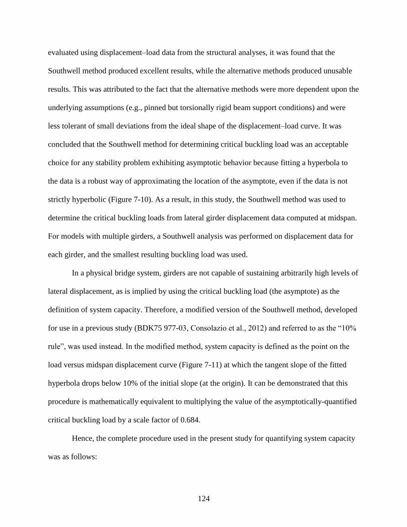
124
evaluated using displacement–load data from the structural analyses, it was found that the
Southwell method produced excellent results, while the alternative methods produced unusable
results. This was attributed to the fact that the alternative methods were more dependent upon the
underlying assumptions (e.g., pinned but torsionally rigid beam support conditions) and were
less tolerant of small deviations from the ideal shape of the displacement–load curve. It was
concluded that the Southwell method for determining critical buckling load was an acceptable
choice for any stability problem exhibiting asymptotic behavior because fitting a hyperbola to
the data is a robust way of approximating the location of the asymptote, even if the data is not
strictly hyperbolic (Figure 7-10). As a result, in this study, the Southwell method was used to
determine the critical buckling loads from lateral girder displacement data computed at midspan.
For models with multiple girders, a Southwell analysis was performed on displacement data for
each girder, and the smallest resulting buckling load was used.
In a physical bridge system, girders are not capable of sustaining arbitrarily high levels of
lateral displacement, as is implied by using the critical buckling load (the asymptote) as the
definition of system capacity. Therefore, a modified version of the Southwell method, developed
for use in a previous study (BDK75 977-03, Consolazio et al., 2012) and referred to as the “10%
rule”, was used instead. In the modified method, system capacity is defined as the point on the
load versus midspan displacement curve (Figure 7-11) at which the tangent slope of the fitted
hyperbola drops below 10% of the initial slope (at the origin). It can be demonstrated that this
procedure is mathematically equivalent to multiplying the value of the asymptotically-quantified
critical buckling load by a scale factor of 0.684.
Hence, the complete procedure used in the present study for quantifying system capacity
was as follows:

125
Wind loads (if any) were applied to the model.
Gravity load was linearly and incrementally increased until the model failed to converge
(i.e., until a system instability occurred).
Displacement vs. load curves were produced for each girder in the system, using the
lateral displacement of the girders at midspan.
Southwell analyses were performed to locate the asymptotes (critical buckling loads) of
the displacement–load curves.
The minimum critical buckling load from among all girders in the model was selected
and multiplied by 0.684 (to apply the 10% rule) to calculate the system capacity.
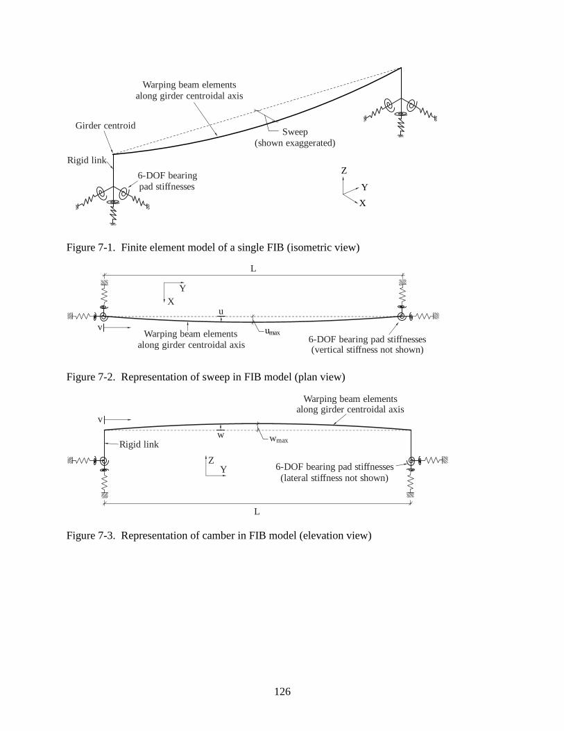
126
Rigid link
Girder centroid
6-DOF bearing
pad stiffnesses
Sweep
(shown exaggerated)
X
Y
Z
Warping beam elements
along girder centroidal axis
Figure 7-1. Finite element model of a single FIB (isometric view)
X
Y
6-DOF bearing pad stiffnesses(vertical stiffness not shown)
v
u
L
Warping beam elements
along girder centroidal axis
umax
Figure 7-2. Representation of sweep in FIB model (plan view)
Rigid link
YZ
wmax
6-DOF bearing pad stiffnesses
(lateral stiffness not shown)
v
L
w
Warping beam elementsalong girder centroidal axis
Figure 7-3. Representation of camber in FIB model (elevation view)
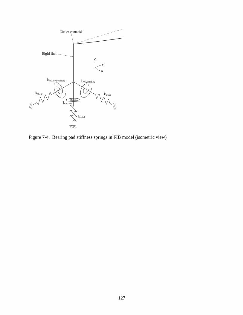
127
Girder centroid
Rigid link
X
Y
Z
kshearkshear
kaxial
ktorsion
kroll,overturning kroll,bending
Figure 7-4. Bearing pad stiffness springs in FIB model (isometric view)
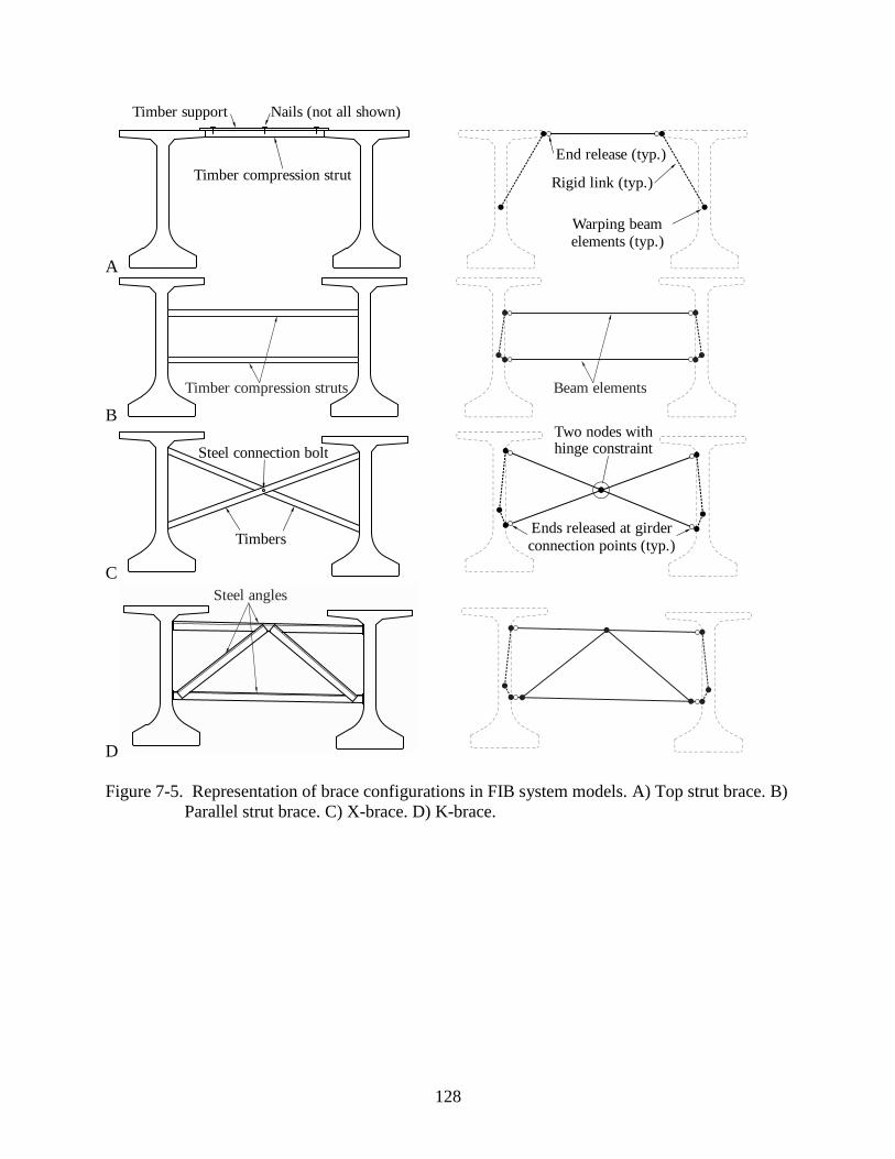
128
A
Timber compression strut
Timber support Nails (not all shown)
Rigid link (typ.)
Warping beam
elements (typ.)
End release (typ.)
B
Timber compression struts Beam elements
C
Timbers
Steel connection bolt
Two nodes with hinge constraint
Ends released at girder
connection points (typ.)
D
Steel angles
Figure 7-5. Representation of brace configurations in FIB system models. A) Top strut brace. B)
Parallel strut brace. C) X-brace. D) K-brace.
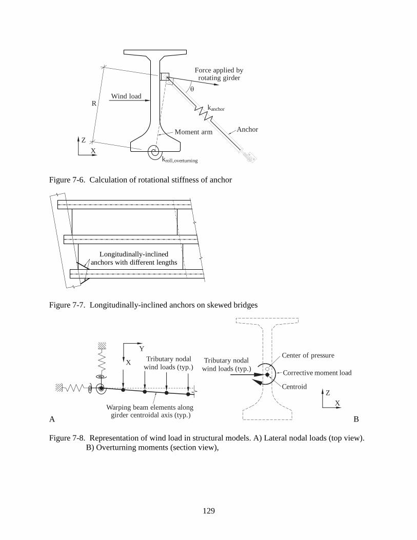
129
Force applied by rotating girder
Wind load
R
kroll,overturning
AnchorMoment arm
kanchor
X
Z
Figure 7-6. Calculation of rotational stiffness of anchor
Longitudinally-inclined
anchors with different lengths
Figure 7-7. Longitudinally-inclined anchors on skewed bridges
A
X
Y
Warping beam elements alonggirder centroidal axis (typ.)
Tributary nodal
wind loads (typ.)
X
Z
Tributary nodal
wind loads (typ.)
Centroid
Center of pressure
Corrective moment load
B
Figure 7-8. Representation of wind load in structural models. A) Lateral nodal loads (top view).
B) Overturning moments (section view),
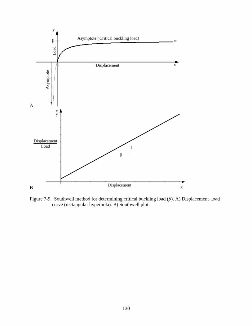
130
A
Displacement
Load
Asymptote (Critical buckling load)
Asy
mp
tote
0
x
y
BDisplacement
Displacement
Load 1
x
yx
Figure 7-9. Southwell method for determining critical buckling load (β). A) Displacement–load
curve (rectangular hyperbola). B) Southwell plot.
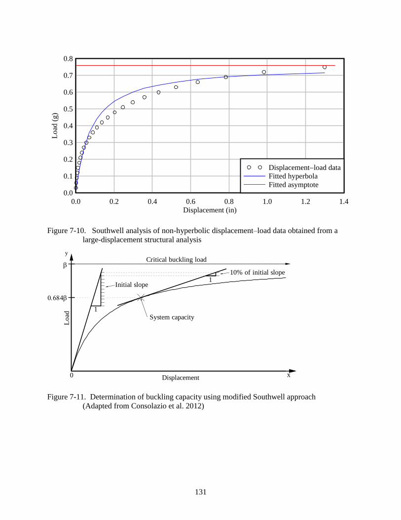
131
Figure 7-10. Southwell analysis of non-hyperbolic displacement–load data obtained from a
large-displacement structural analysis
Displacement
Load
0
Initial slope
System capacity
Critical buckling load
1
110% of initial slope
y
x
Figure 7-11. Determination of buckling capacity using modified Southwell approach
(Adapted from Consolazio et al. 2012)
Displacement (in)
Lo
ad (
g)
0.0 0.2 0.4 0.6 0.8 1.0 1.2 1.4
0.0
0.1
0.2
0.3
0.4
0.5
0.6
0.7
0.8
Displacementload data
Fitted hyperbola
Fitted asymptote
132
CHAPTER 8
PARAMETRIC STUDY OF INDIVIDUAL BRIDGE GIRDERS
8.1 Introduction
During the bridge construction process, the stage at which wind loading is often most
critical is when the first girder is erected. At this stage there are no other girders to brace against,
hence the initial girder cannot be braced at interior points, and can only be anchored to the pier at
the ends. For bridge designs in which girder stability is a primary concern, girder erection can
sometimes be scheduled to minimize the exposure period for the initial girder, so that it is
statistically unlikely that peak wind forces will occur. However, meeting such a schedule is not
always feasible. For example, strong afternoon thunderstorms can form rapidly in Florida during
the summer months. In such situations, it is important to be able to assess, in advance, whether
anchor bracing will be needed to prevent girder collapse under the effects of thunderstorm-force
winds.
To investigate this scenario, a parametric study was performed, using finite element
models of single Florida-I Beams (FIBs) over a range of span lengths, both with and without
anchor bracing in place. For each model, the system capacity was evaluated several times at
different wind pressures, iterating until the capacity was within 1% of 1 g (i.e., the capacity-to-
demand ratio was approximately unity). For each such case, the resulting wind pressure was
termed the wind capacity of that girder, representing the maximum wind load that can be
sustained by the girder without collapsing. Using the results of the parametric study, equations
were developed for predicting the wind capacity of a single FIB.
8.2 Selection of Parameters
The girder parameters that were varied in the parametric study were as follows:
FIB cross-section depth (in)
Span length (ft)
133
Rotational stiffness of anchor bracing (kip-ft/rad)
All eight (8) standard FIB cross-sections were included in the study, with depths ranging from 36
in. to 96 in. For each FIB, wind capacity analyses were performed for every combination of span
length and anchor stiffness, sampled from the values listed in Table 8-1. Bridge grade was also
considered as a potential parameter, but was rejected after preliminary analyses showed that it
had a negligible effect on wind capacity. Therefore, all analyses were performed on girder
models with a level (0%) grade.
Maximum and minimum span lengths used in the parametric study were based on design
aids included in Instructions for Design Standard No. 20010: Prestressed Florida-I Beams (IDS
20010; FDOT, 2012b), which provides estimated span lengths (Table 8-2) for FIBs with
different lateral spacings, based on representative bridge design calculations. Maximum lengths
were based on a spacing of 6 ft and an environment classified as “Moderately Aggressive”, while
minimum lengths assumed a 12-ft spacing and an “Extremely Aggressive” environment. To
ensure that the considered length ranges included all reasonable beam designs, the basic ranges
taken from IDS 20010 were extended by 3 ft on each end, and then extended further so that
range limits were even multiples of 5 ft. The parametric study included span lengths chosen at 5-
ft intervals over the final ranges.
A survey of bracing designs used in girder bridges constructed in Florida revealed
anchors with equivalent rotational stiffnesses ranging from 500 to 50,000 kip-ft/rad. However, it
was found that when large anchor stiffnesses were included in girder models, particularly for
shorter span, shallower girders less prone to instability, the models no longer exhibited a normal
buckling response. In moderate cases, this caused the computed wind capacity to be artificially
inflated, and, in the most extreme cases, the wind capacity could not be computed at all (i.e., the
134
wind pressures required to initiate girder instability under self-weight were so large—well
beyond material strength limits—that the displacement–load results ceased to be
characteristically asymptotic and the modified Southwell analysis method was no longer
applicable). Therefore, a maximum practical anchor stiffness (at which a wind capacity could be
computed) was established for each FIB through trial and error, and the parametric study
included ten (10) evenly-distributed stiffness values up to and including that maximum (in
addition to the unanchored case, with zero anchor stiffness).
In practice, the maximum practical anchor stiffness was smaller for FIBs with shorter
span lengths, but it was not feasible to determine a different maximum stiffness for every FIB at
every span length. Instead, a maximum anchor stiffness was established based on the maximum
span length for each FIB, and the parametric study was carried out with the understanding that
not every combination of parameters would result in a computable wind capacity. At the
minimum span length, it was common to obtain results for only the lowest 4 or 5 stiffness values.
There were also two cases (the 215-ft, 96″ FIB with anchor stiffnesses of 0 and 410 kip-ft/rad)
for which a meaningful wind capacity did not exist because the girder was inherently unstable,
collapsing under less than 1 g in the absence of any wind. In total, 781 wind capacity analyses
were attempted in the parametric study, of which 471 produced results. (The 471 computed wind
capacities included the some of the artificially-inflated values described above. Identification and
rejection of those data points is discussed in more detail later in the chapter.)
8.3 Results
Wind capacities computed from the parametric study are summarized in Figure 8-1.
Visually, the data are divided into eight (8) major groups, each of which corresponds to one of
the tested FIB cross-sections, ranging from the 36″ FIB (cases 1–48) to the 96″ FIB (cases 405–
471). Each group contains several subgroups—visually identifiable as diagonal lines of
135
consecutive data points—that represent the wind capacities computed for a single span length (at
several different anchor stiffnesses). The ‘cloud’ of outlier points, located well above the
subgroups, consists of the artificially-inflated wind-capacities that occurred at higher anchor
stiffnesses.
The results of the parametric study were used to develop an equation for estimating the
wind capacity (Pmax) of any FIB. This was accomplished by first developing an equation for the
wind capacity of an unanchored FIB (Pmax,0), in terms of the section depth (D) and span length
(L) and then determining a linear correction factor that incorporated the effect of the anchor
stiffness (k).
8.3.1 Wind Capacity of a Single Unanchored Girder
The relationship between wind capacity and span length for unanchored FIBs is plotted in
Figure 8-2. It is evident from the plot that span length is the strongest predictor of wind capacity,
which declines sharply as span length increases. Wind capacity is also reduced when the girder
depth increases, which can be attributed to the larger sail area (projected area) over which the
wind pressure is applied. There is no data for the 215-ft 96″ FIB because, as noted earlier, its
capacity-to-demand ratio was less than 1 prior to the application of wind. In the final equation,
this situation will be indicated by producing a negative wind capacity value.
The functional form found to be the closest fit to each of the FIB curves was an
exponential relationship:
bxy ae c (8-1)
where a, b, and c are fitting parameters. For each FIB, a separate exponential curve-fit was
performed to relate wind capacity to span length, L. It was found that the value of b in these
curve-fits was approximately constant, while the variance in the a and c terms had a similar
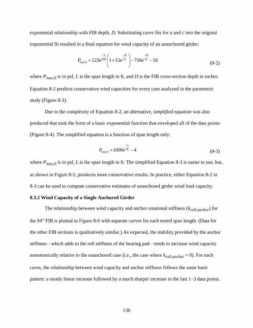
136
exponential relationship with FIB depth, D. Substituting curve fits for a and c into the original
exponential fit resulted in a final equation for wind capacity of an unanchored girder:
100 16220 123 1 15 750 16
L DD
max,P e e e
(8-2)
where Pmax,0 is in psf, L is the span length in ft, and D is the FIB cross-section depth in inches.
Equation 8-2 predicts conservative wind capacities for every case analyzed in the parametric
study (Figure 8-3).
Due to the complexity of Equation 8-2, an alternative, simplified equation was also
produced that took the form of a basic exponential function that enveloped all of the data points
(Figure 8-4). The simplified equation is a function of span length only:
38max,0 1000 4
L
P e
(8-3)
where Pmax,0 is in psf, L is the span length in ft. The simplified Equation 8-3 is easier to use, but,
as shown in Figure 8-5, produces more conservative results. In practice, either Equation 8-2 or
8-3 can be used to compute conservative estimates of unanchored girder wind load capacity.
8.3.2 Wind Capacity of a Single Anchored Girder
The relationship between wind capacity and anchor rotational stiffness (kroll,anchor) for
the 84″ FIB is plotted in Figure 8-6 with separate curves for each tested span length. (Data for
the other FIB sections is qualitatively similar.) As expected, the stability provided by the anchor
stiffness—which adds to the roll stiffness of the bearing pad—tends to increase wind capacity
monotonically relative to the unanchored case (i.e., the case where kroll,anchor = 0). For each
curve, the relationship between wind capacity and anchor stiffness follows the same basic
pattern: a steady linear increase followed by a much sharper increase in the last 1–3 data points.
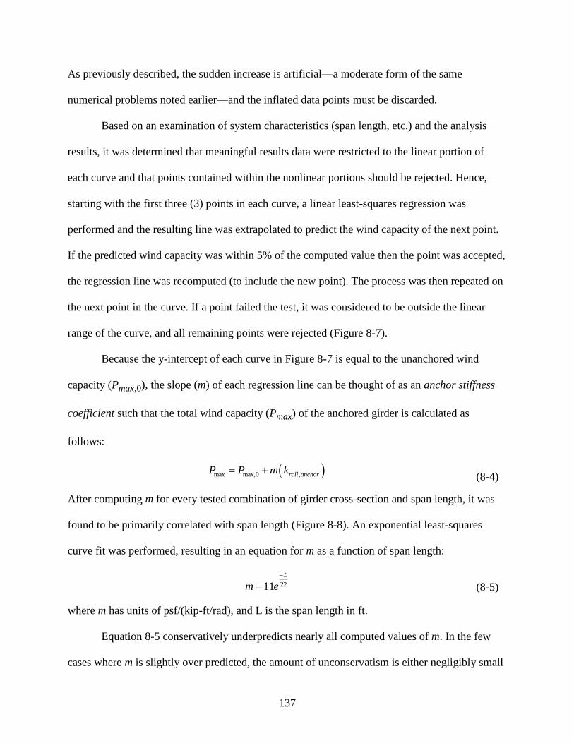
137
As previously described, the sudden increase is artificial—a moderate form of the same
numerical problems noted earlier—and the inflated data points must be discarded.
Based on an examination of system characteristics (span length, etc.) and the analysis
results, it was determined that meaningful results data were restricted to the linear portion of
each curve and that points contained within the nonlinear portions should be rejected. Hence,
starting with the first three (3) points in each curve, a linear least-squares regression was
performed and the resulting line was extrapolated to predict the wind capacity of the next point.
If the predicted wind capacity was within 5% of the computed value then the point was accepted,
the regression line was recomputed (to include the new point). The process was then repeated on
the next point in the curve. If a point failed the test, it was considered to be outside the linear
range of the curve, and all remaining points were rejected (Figure 8-7).
Because the y-intercept of each curve in Figure 8-7 is equal to the unanchored wind
capacity (Pmax,0), the slope (m) of each regression line can be thought of as an anchor stiffness
coefficient such that the total wind capacity (Pmax) of the anchored girder is calculated as
follows:
max max,0 ,roll anchorP P m k (8-4)
After computing m for every tested combination of girder cross-section and span length, it was
found to be primarily correlated with span length (Figure 8-8). An exponential least-squares
curve fit was performed, resulting in an equation for m as a function of span length:
2211L
m e
(8-5)
where m has units of psf/(kip-ft/rad), and L is the span length in ft.
Equation 8-5 conservatively underpredicts nearly all computed values of m. In the few
cases where m is slightly over predicted, the amount of unconservatism is either negligibly small
138
or is compensated for by conservatism in the determination of Pmax,0. As a result, the wind
capacity of a single anchored girder can be predicted as follows:
22max max,0 ,11
L
roll anchorP P e k
(8-6)
where kroll,anchor is in kip-ft/rad, L is the span length in ft, and Pmax,0 is in psf and is calculated
using either Equation 8-2 or 8-3. When Equation 8-2 is used, the majority of wind capacities
predicted by Equation 8-6 fall within 10% (see Figure 8-6) of the corresponding values
computed in the parametric study.
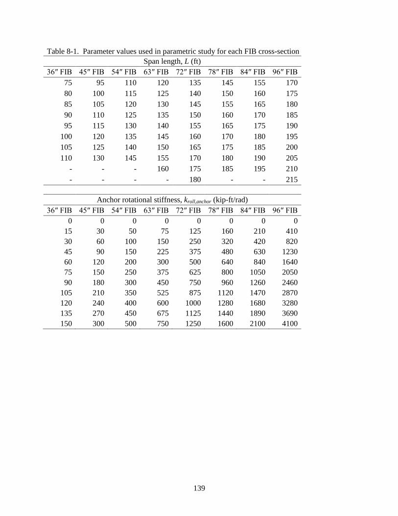
139
Table 8-1. Parameter values used in parametric study for each FIB cross-section
Span length, L (ft)
36″ FIB 45″ FIB 54″ FIB 63″ FIB 72″ FIB 78″ FIB 84″ FIB 96″ FIB
75 95 110 120 135 145 155 170
80 100 115 125 140 150 160 175
85 105 120 130 145 155 165 180
90 110 125 135 150 160 170 185
95 115 130 140 155 165 175 190
100 120 135 145 160 170 180 195
105 125 140 150 165 175 185 200
110 130 145 155 170 180 190 205
- - - 160 175 185 195 210
- - - - 180 - - 215
Anchor rotational stiffness, kroll,anchor (kip-ft/rad)
36″ FIB 45″ FIB 54″ FIB 63″ FIB 72″ FIB 78″ FIB 84″ FIB 96″ FIB
0 0 0 0 0 0 0 0
15 30 50 75 125 160 210 410
30 60 100 150 250 320 420 820
45 90 150 225 375 480 630 1230
60 120 200 300 500 640 840 1640
75 150 250 375 625 800 1050 2050
90 180 300 450 750 960 1260 2460
105 210 350 525 875 1120 1470 2870
120 240 400 600 1000 1280 1680 3280
135 270 450 675 1125 1440 1890 3690
150 300 500 750 1250 1600 2100 4100
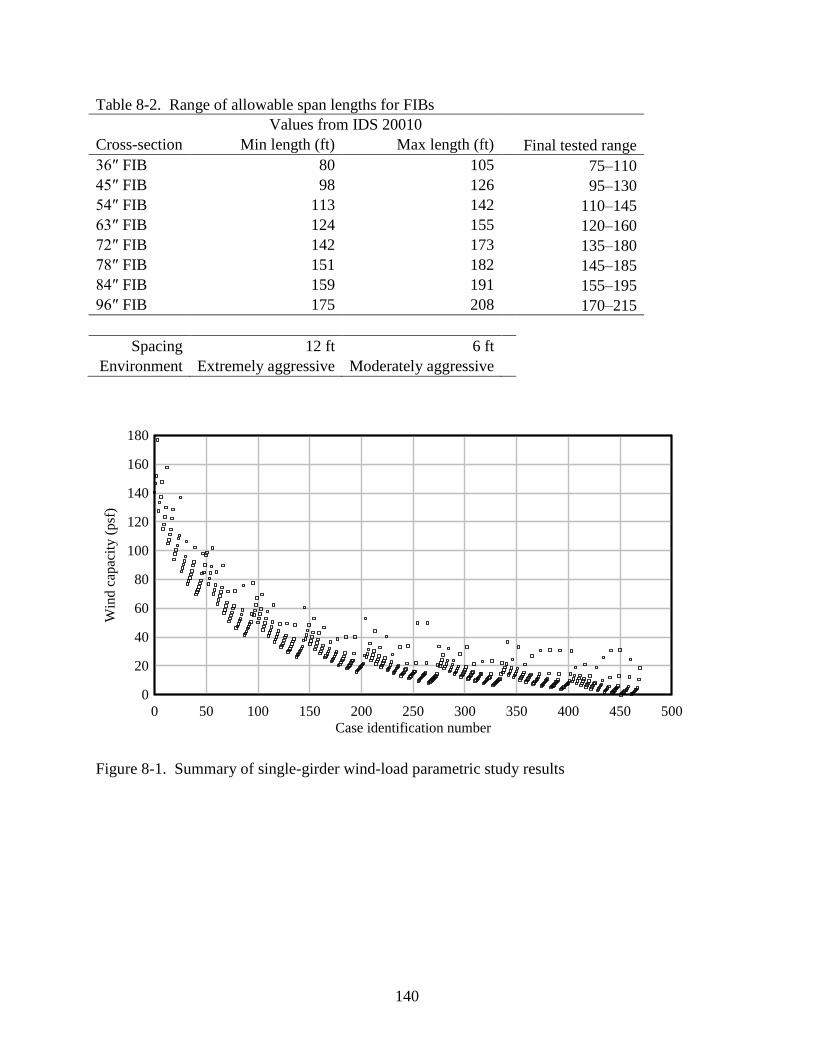
140
Table 8-2. Range of allowable span lengths for FIBs
Values from IDS 20010
Cross-section Min length (ft) Max length (ft)
Final tested range
36″ FIB 80 105
75–110
45″ FIB 98 126
95–130
54″ FIB 113 142
110–145
63″ FIB 124 155
120–160
72″ FIB 142 173
135–180
78″ FIB 151 182
145–185
84″ FIB 159 191
155–195
96″ FIB 175 208
170–215
Spacing 12 ft 6 ft
Environment Extremely aggressive Moderately aggressive
Figure 8-1. Summary of single-girder wind-load parametric study results
Case identification number
Win
d c
apac
ity
(p
sf)
0 50 100 150 200 250 300 350 400 450 500
0
20
40
60
80
100
120
140
160
180
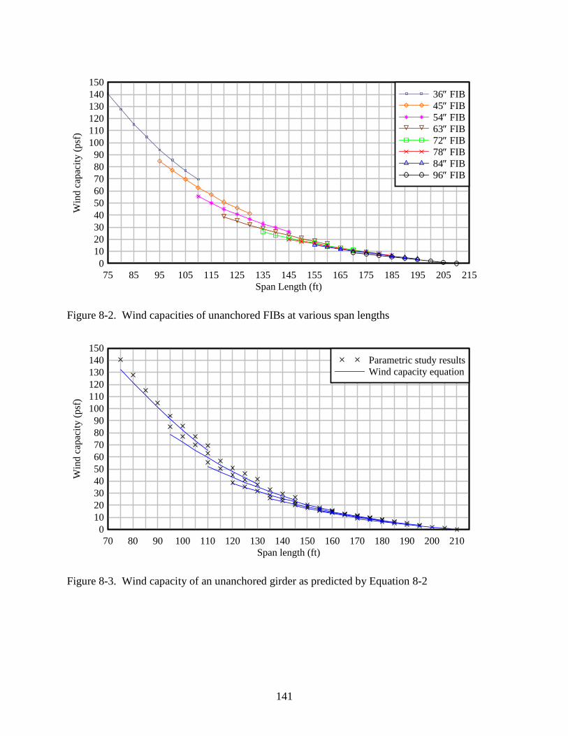
141
Figure 8-2. Wind capacities of unanchored FIBs at various span lengths
Figure 8-3. Wind capacity of an unanchored girder as predicted by Equation 8-2
Span Length (ft)
Win
d c
apac
ity
(p
sf)
75 85 95 105 115 125 135 145 155 165 175 185 195 205 215
0
10
20
30
40
50
60
70
80
90
100
110
120
130
140
150
36 FIB
45 FIB
54 FIB
63 FIB
72 FIB
78 FIB
84 FIB
96 FIB
Span length (ft)
Win
d c
apac
ity
(p
sf)
70 80 90 100 110 120 130 140 150 160 170 180 190 200 210
0
10
20
30
40
50
60
70
80
90
100
110
120
130
140
150
Parametric study results
Wind capacity equation
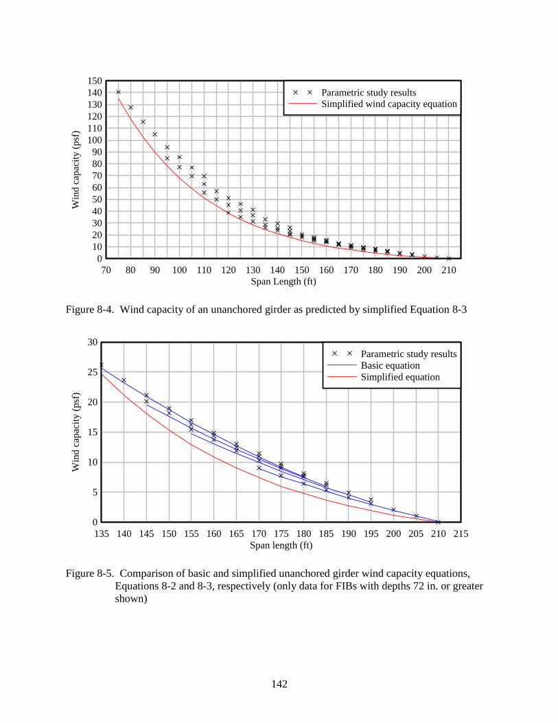
142
Figure 8-4. Wind capacity of an unanchored girder as predicted by simplified Equation 8-3
Figure 8-5. Comparison of basic and simplified unanchored girder wind capacity equations,
Equations 8-2 and 8-3, respectively (only data for FIBs with depths 72 in. or greater
shown)
Span Length (ft)
Win
d c
apac
ity (
psf
)
70 80 90 100 110 120 130 140 150 160 170 180 190 200 210
0
10
20
30
40
50
60
70
80
90
100
110
120
130
140
150
Parametric study results
Simplified wind capacity equation
Span length (ft)
Win
d c
apac
ity
(p
sf)
135 140 145 150 155 160 165 170 175 180 185 190 195 200 205 210 215
0
5
10
15
20
25
30
Parametric study results
Basic equation
Simplified equation
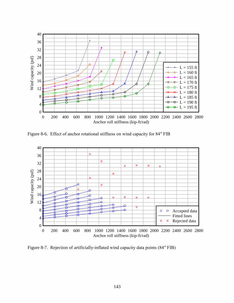
143
Figure 8-6. Effect of anchor rotational stiffness on wind capacity for 84″ FIB
Figure 8-7. Rejection of artificially-inflated wind capacity data points (84″ FIB)
Anchor roll stiffness (kip-ft/rad)
Win
d c
apac
ity (
psf
)
0 200 400 600 800 1000 1200 1400 1600 1800 2000 2200 2400 2600 2800
0
4
8
12
16
20
24
28
32
36
40
L = 155 ft
L = 160 ft
L = 165 ft
L = 170 ft
L = 175 ft
L = 180 ft
L = 185 ft
L = 190 ft
L = 195 ft
Anchor roll stiffness (kip-ft/rad)
Win
d c
apac
ity (
psf
)
0 200 400 600 800 1000 1200 1400 1600 1800 2000 2200 2400 2600 2800
0
4
8
12
16
20
24
28
32
36
40
Accepted data
Fitted lines
Rejected data
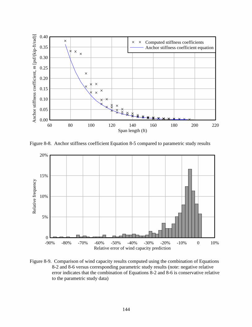
144
Figure 8-8. Anchor stiffness coefficient Equation 8-5 compared to parametric study results
Figure 8-9. Comparison of wind capacity results computed using the combination of Equations
8-2 and 8-6 versus corresponding parametric study results (note: negative relative
error indicates that the combination of Equations 8-2 and 8-6 is conservative relative
to the parametric study data)
Span length (ft)
An
cho
r st
iffn
ess
coef
fici
ent,
m [
psf
/(k
ip-f
t/ra
d)]
60 80 100 120 140 160 180 200 220
0.00
0.05
0.10
0.15
0.20
0.25
0.30
0.35
0.40
Computed stiffness coefficients
Anchor stiffness coefficient equation
Relative error of wind capacity prediction
Rel
ativ
e fr
equen
cy
-90% -80% -70% -60% -50% -40% -30% -20% -10% 0 10%
0
5%
10%
15%
20%
145
CHAPTER 9
PARAMETRIC STUDY OF BRACED MULTI-GIRDER SYSTEMS
9.1 Preliminary Sensitivity Studies
Fully characterizing a braced multi-girder system requires a large number of geometric
parameters. Consequently, conducting parametric studies in which all possible combinations of
these parameters are considered (even if only a few discrete values are selected per parameter)
would require hundreds of thousands of analyses to be performed. To avoid such a situation,
several limited-scope preliminary sensitivity studies were performed to help guide the design of
efficient final parametric studies. As a result of these preliminary investigations—the details of
which will be omitted here for brevity—several system parameters were identified as having
negligible influence on system capacity. Consequently, these parameters were not varied in the
final parametric studies. The parameters were:
Bridge grade: All analyses were performed on girder models with level (0%) grade.
Cross-slope: Multi-girder models had a default −2% cross-slope.
Location of anchored girder in bridge cross-section: In cases where anchors were
included, they were always attached to the most leeward (downwind) girder.
The preliminary studies also revealed that braces were naturally divided into two
categories that had very different effects on system behavior: strut braces and moment-resisting
braces. As a result, separate parametric studies were performed for each brace category.
9.1.1 Strut Braces
Top struts and parallel struts (Figure 9-1) are both examples of strut braces, which
include (but are not limited to) all brace designs consisting solely of horizontal compression
members. Somewhat surprisingly, it was found that all strut brace designs are essentially
interchangeable with regard to lateral stability. That is, a girder system braced with top struts has
the same capacity as an otherwise identical system braced instead with parallel struts (or any
146
other type of strut brace). As a result, the capacity of a strut-braced system is also insensitive to
girder spacing (which only affects the length—and thus the axial stiffness—of the strut
members). Additionally, there is no measurable gain in system capacity that results from the
installation of struts at interior brace points. End bracing alone is sufficient to mobilize all of the
girder buckling capacity that can be provided by strut braces. It is also worth noting that the
capacity of a strut-braced system decreases as additional girders are added.
Strut braces can be defined (or identified) by their lack of resistance to girder
overturning. In a small-displacement (geometrically linear) analysis of a system with zero
bearing pad rotational stiffness, a strut with ideal pin connections forms a collapse mechanism
(Figure 9-2) that allows the connected girders to rotate freely in unison. Therefore, struts can
only provide stability by coupling the girders together, and resistance to collapse is primarily
provided by the roll stiffness of the anchors and, to a lesser extent, the roll stiffness of the
bearing pad supports. This behavior is also the reason that adding girders to a system reduces
stability: each new girder adds additional wind load (and additional bearing pad stiffness) while
the number of anchors remains constant.
9.1.2 Moment-Resisting Braces
X-braces and K-braces (Figure 9-3) are both examples of moment-resisting braces, which
are capable of resisting girder overturning. Unlike struts, the system capacity provided by
different moment-resisting brace designs varies significantly, and capacity can be increased by
the installation of braces at interior brace points. Systems with moment-resisting braces become
more stable as additional girders are added; hence a two-girder system is nearly always the most
unstable bridge cross-section possible. In the presence of moment-resisting bracing, the
additional roll stiffness and stability provided by anchors is typically negligible.
147
9.2 Modeling of Bridge Skew and Wind Load
In a braced system of girders, the introduction of bridge skew causes the girders to
become staggered longitudinally. This affects system capacity in two ways (Figure 9-4):
Brace placement: Because girders are installed perpendicular to the girder axes (per
Design Standard No. 20005: Prestressed I-Beam Temporary Bracing, FDOT, 2012a), the
region within which braces can be placed is smaller (shorter) than the span length of the
girders. As a result, girder stability can increase due to the reduced distance between
brace points.
Incomplete shielding: In a skewed system, none of the girders are completed shielded
with respect to wind load. Rather, an end portion of each girder is exposed to full
(unshielded) wind pressure. The aerodynamic properties of the exposed end region have
not been measured in a wind tunnel, so specific ‘edge effects’ that may result from the
presence of upwind girders are unknown.
The magnitude of both of these effects is a function of the girder offset length (Loffset), (Figure
9-4) which is dependent on both skew angle and girder spacing.
Conducting wind tunnel testing to experimentally quantify the effects of skew on girder-
end shielding was outside the scope of this study. Consequently, the non-uniform wind pressure
distribution shown for leeward girders in Figure 9-4b is an approximation based on engineering
judgment. Lacking wind tunnel confirmation of this approximation, it was deemed unwarranted
to model this distribution in detail in the parametric studies. Instead, a simplified, but statically
similar, representation was used in which the wind load on each girder was modeled as a single,
weighted-average uniform pressure along the entire length of the girder. The uniform wind load
applied to each partially-shielded girder (P) was computed as a weighted average of the shielded
and unshielded wind loads, as follows:
offset offset
U S
L L LP P P
L L
(9-1)
where PU is the unshielded wind load (on the windward girder), PS is the shielded wind load, L
is the girder length, and Loffset is the length of girder offset produced by skew.

148
9.3 Selection of Parameters for Strut Brace Parametric Study
System parameters that were varied in the strut brace parametric study were as follows:
FIB cross-section depth (in)
Span length (ft)
Number of girders
Rotational stiffness of anchor bracing (kip-ft/rad)
Wind pressure (psf)
Skew angle (deg)
All eight (8) standard FIB cross-sections were included in the study, with depths ranging from 36
in. to 96 in. For each FIB, capacity analyses were performed for every combination of span
length, anchor stiffness, wind pressure, skew angle, and number of girders, sampled from the
values listed in Table 9-1, for a total of 37,800 analyses.
Maximum and minimum span lengths were based on the same span length ranges used
for the single girder study (see Chapter 8). However, to reduce the number of analyses to a
feasible level, the study used lengths chosen at 10-ft intervals instead of 5-ft intervals. When
necessary, the upper limit of the range was increased by 5 ft so that the total range was evenly
divisible into 10-ft intervals. Similarly, the maximum anchor stiffnesses were the same that were
used for the single-girder study, but five (5) evenly distributed values were used instead of ten
(10).
As noted earlier, preliminary analyses demonstrated that the capacity of a strut-braced
system continues to decrease as more girders are added. A practical upper bound of nine (9)
girders was selected to be representative of wide bridge cross-sections while simultaneously
limiting the finite element models to a manageable size (number of nodes, elements, and degrees
of freedom).
Wind pressure loads were applied to the girders using the shielding pattern proposed in
Chapter 5, and using the wind pressures listed in Table 9-1. Wind pressures specified in the table
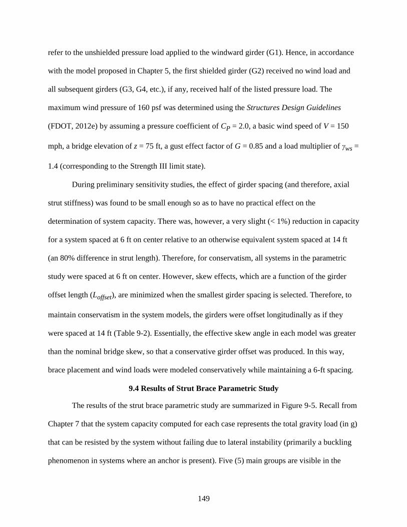
149
refer to the unshielded pressure load applied to the windward girder (G1). Hence, in accordance
with the model proposed in Chapter 5, the first shielded girder (G2) received no wind load and
all subsequent girders (G3, G4, etc.), if any, received half of the listed pressure load. The
maximum wind pressure of 160 psf was determined using the Structures Design Guidelines
(FDOT, 2012e) by assuming a pressure coefficient of CP = 2.0, a basic wind speed of V = 150
mph, a bridge elevation of z = 75 ft, a gust effect factor of G = 0.85 and a load multiplier of γws =
1.4 (corresponding to the Strength III limit state).
During preliminary sensitivity studies, the effect of girder spacing (and therefore, axial
strut stiffness) was found to be small enough so as to have no practical effect on the
determination of system capacity. There was, however, a very slight (< 1%) reduction in capacity
for a system spaced at 6 ft on center relative to an otherwise equivalent system spaced at 14 ft
(an 80% difference in strut length). Therefore, for conservatism, all systems in the parametric
study were spaced at 6 ft on center. However, skew effects, which are a function of the girder
offset length (Loffset), are minimized when the smallest girder spacing is selected. Therefore, to
maintain conservatism in the system models, the girders were offset longitudinally as if they
were spaced at 14 ft (Table 9-2). Essentially, the effective skew angle in each model was greater
than the nominal bridge skew, so that a conservative girder offset was produced. In this way,
brace placement and wind loads were modeled conservatively while maintaining a 6-ft spacing.
9.4 Results of Strut Brace Parametric Study
The results of the strut brace parametric study are summarized in Figure 9-5. Recall from
Chapter 7 that the system capacity computed for each case represents the total gravity load (in g)
that can be resisted by the system without failing due to lateral instability (primarily a buckling
phenomenon in systems where an anchor is present). Five (5) main groups are visible in the

150
summary of results, each of which corresponds to a different wind pressure value (in increasing
order from 0 to 160 psf). Each group contains eight (8) subgroups—corresponding to the tested
FIB cross-sections—each of which is composed of five (5) or six (6) adjacent groups of data
points arranged in a steep diagonal line—corresponding to the tested span lengths. Variation
within the data groups reflects the relatively small effects of anchor stiffness and the number of
girders in the system.
The results were used to develop an equation for capacity (C) of a strut-braced system of
FIBs. This was accomplished by first determining the baseline capacity of an unanchored system
of two girders in zero wind conditions (C0), and then developing correction factors to adjust the
system capacity upward in response to anchor stiffness and downward in response to wind load
and the erection of additional girders. A wide range of FIB system capacities (up to 10 g) were
present in the parametric study results, but under heavy wind, a large number of systems also had
a capacity of 0, which the capacity equations indicate by computing a negative capacity value.
Two techniques were used to simplify interpretation of the parametric study results. The
large number of interacting parameters and the wide range of the capacity values made it
impractical to produce equations with a uniform level of conservatism throughout the data set.
Therefore, capacity prediction equations were considered satisfactory if they conservatively
enveloped 95% of the data points, and as long as none of the unconservative cases were more
than 5% in error with regard to computed capacity. Also, while it was important that the
equations be accurate and not overly conservative for systems where stability was likely to
control design, the same characteristics are less important for extremely stable systems.
Therefore, when appropriate, to simplify the data interpretation process systems with capacities
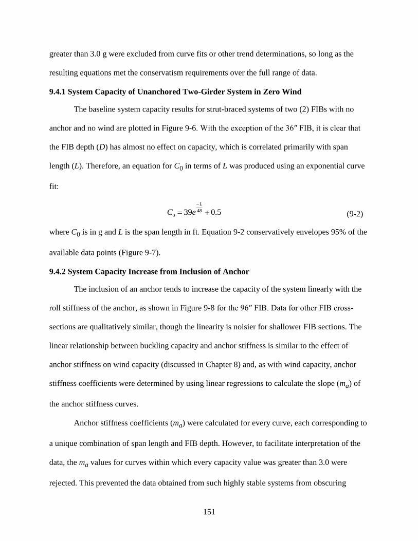
151
greater than 3.0 g were excluded from curve fits or other trend determinations, so long as the
resulting equations met the conservatism requirements over the full range of data.
9.4.1 System Capacity of Unanchored Two-Girder System in Zero Wind
The baseline system capacity results for strut-braced systems of two (2) FIBs with no
anchor and no wind are plotted in Figure 9-6. With the exception of the 36″ FIB, it is clear that
the FIB depth (D) has almost no effect on capacity, which is correlated primarily with span
length (L). Therefore, an equation for C0 in terms of L was produced using an exponential curve
fit:
480 39 0.5
L
C e
(9-2)
where C0 is in g and L is the span length in ft. Equation 9-2 conservatively envelopes 95% of the
available data points (Figure 9-7).
9.4.2 System Capacity Increase from Inclusion of Anchor
The inclusion of an anchor tends to increase the capacity of the system linearly with the
roll stiffness of the anchor, as shown in Figure 9-8 for the 96″ FIB. Data for other FIB cross-
sections are qualitatively similar, though the linearity is noisier for shallower FIB sections. The
linear relationship between buckling capacity and anchor stiffness is similar to the effect of
anchor stiffness on wind capacity (discussed in Chapter 8) and, as with wind capacity, anchor
stiffness coefficients were determined by using linear regressions to calculate the slope (ma) of
the anchor stiffness curves.
Anchor stiffness coefficients (ma) were calculated for every curve, each corresponding to
a unique combination of span length and FIB depth. However, to facilitate interpretation of the
data, the ma values for curves within which every capacity value was greater than 3.0 were
rejected. This prevented the data obtained from such highly stable systems from obscuring
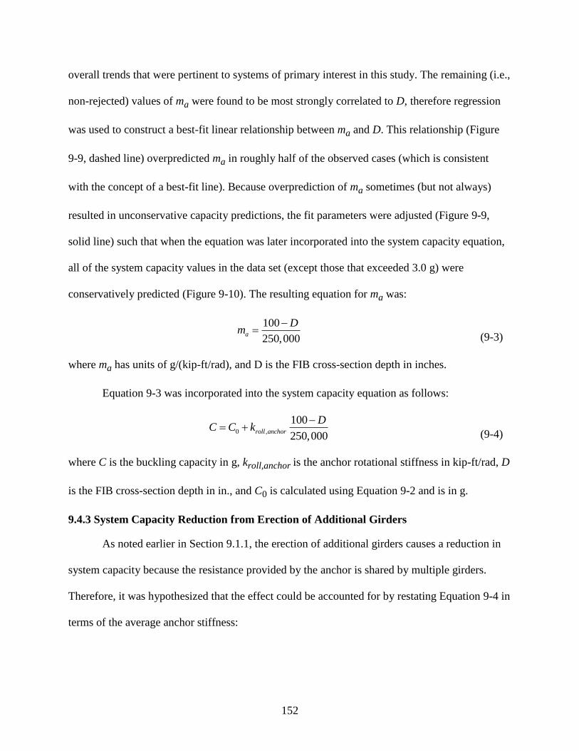
152
overall trends that were pertinent to systems of primary interest in this study. The remaining (i.e.,
non-rejected) values of ma were found to be most strongly correlated to D, therefore regression
was used to construct a best-fit linear relationship between ma and D. This relationship (Figure
9-9, dashed line) overpredicted ma in roughly half of the observed cases (which is consistent
with the concept of a best-fit line). Because overprediction of ma sometimes (but not always)
resulted in unconservative capacity predictions, the fit parameters were adjusted (Figure 9-9,
solid line) such that when the equation was later incorporated into the system capacity equation,
all of the system capacity values in the data set (except those that exceeded 3.0 g) were
conservatively predicted (Figure 9-10). The resulting equation for ma was:
100
250,000a
Dm
(9-3)
where ma has units of g/(kip-ft/rad), and D is the FIB cross-section depth in inches.
Equation 9-3 was incorporated into the system capacity equation as follows:
0 ,
100
250,000roll anchor
DC C k
(9-4)
where C is the buckling capacity in g, kroll,anchor is the anchor rotational stiffness in kip-ft/rad, D
is the FIB cross-section depth in in., and C0 is calculated using Equation 9-2 and is in g.
9.4.3 System Capacity Reduction from Erection of Additional Girders
As noted earlier in Section 9.1.1, the erection of additional girders causes a reduction in
system capacity because the resistance provided by the anchor is shared by multiple girders.
Therefore, it was hypothesized that the effect could be accounted for by restating Equation 9-4 in
terms of the average anchor stiffness:
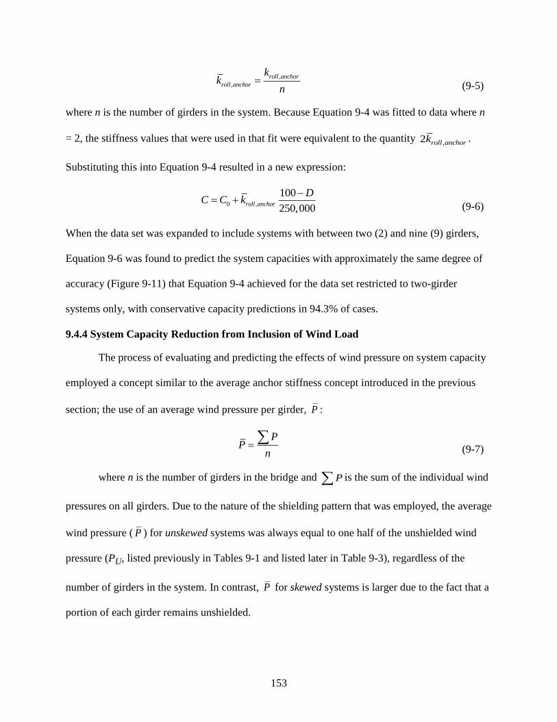
153
,
,
roll anchor
roll anchor
kk
n
(9-5)
where n is the number of girders in the system. Because Equation 9-4 was fitted to data where n
= 2, the stiffness values that were used in that fit were equivalent to the quantity ,2 roll anchork .
Substituting this into Equation 9-4 resulted in a new expression:
0 ,
100
250,000roll anchor
DC C k
(9-6)
When the data set was expanded to include systems with between two (2) and nine (9) girders,
Equation 9-6 was found to predict the system capacities with approximately the same degree of
accuracy (Figure 9-11) that Equation 9-4 achieved for the data set restricted to two-girder
systems only, with conservative capacity predictions in 94.3% of cases.
9.4.4 System Capacity Reduction from Inclusion of Wind Load
The process of evaluating and predicting the effects of wind pressure on system capacity
employed a concept similar to the average anchor stiffness concept introduced in the previous
section; the use of an average wind pressure per girder, P :
PP
n
(9-7)
where n is the number of girders in the bridge and P is the sum of the individual wind
pressures on all girders. Due to the nature of the shielding pattern that was employed, the average
wind pressure ( P ) for unskewed systems was always equal to one half of the unshielded wind
pressure (PU, listed previously in Tables 9-1 and listed later in Table 9-3), regardless of the
number of girders in the system. In contrast, P for skewed systems is larger due to the fact that a
portion of each girder remains unshielded.
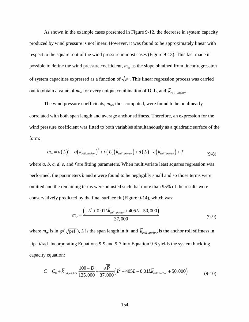
154
As shown in the example cases presented in Figure 9-12, the decrease in system capacity
produced by wind pressure is not linear. However, it was found to be approximately linear with
respect to the square root of the wind pressure in most cases (Figure 9-13). This fact made it
possible to define the wind pressure coefficient, mw as the slope obtained from linear regression
of system capacities expressed as a function of P . This linear regression process was carried
out to obtain a value of mw for every unique combination of D, L, and ,roll anchork .
The wind pressure coefficients, mw, thus computed, were found to be nonlinearly
correlated with both span length and average anchor stiffness. Therefore, an expression for the
wind pressure coefficient was fitted to both variables simultaneously as a quadratic surface of the
form:
22
, , ,w roll anchor roll anchor roll anchorm a L b k c L k d L e k f (9-8)
where a, b, c, d, e, and f are fitting parameters. When multivariate least squares regression was
performed, the parameters b and e were found to be negligibly small and so those terms were
omitted and the remaining terms were adjusted such that more than 95% of the results were
conservatively predicted by the final surface fit (Figure 9-14), which was:
2
,0.01 405 50,000
37,000
roll anchor
w
L Lk Lm
(9-9)
where mw is in g/( psf ), L is the span length in ft, and ,roll anchork is the anchor roll stiffness in
kip-ft/rad. Incorporating Equations 9-9 and 9-7 into Equation 9-6 yields the system buckling
capacity equation:
2
0 , ,
100405 0.01 50,000
125,000 37,000roll anchor roll anchor
D PC C k L L Lk
(9-10)
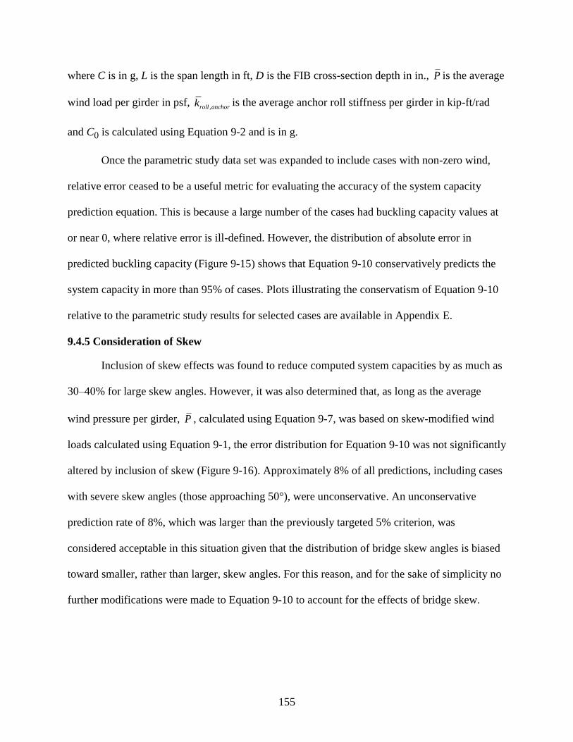
155
where C is in g, L is the span length in ft, D is the FIB cross-section depth in in., P is the average
wind load per girder in psf, ,roll anchork is the average anchor roll stiffness per girder in kip-ft/rad
and C0 is calculated using Equation 9-2 and is in g.
Once the parametric study data set was expanded to include cases with non-zero wind,
relative error ceased to be a useful metric for evaluating the accuracy of the system capacity
prediction equation. This is because a large number of the cases had buckling capacity values at
or near 0, where relative error is ill-defined. However, the distribution of absolute error in
predicted buckling capacity (Figure 9-15) shows that Equation 9-10 conservatively predicts the
system capacity in more than 95% of cases. Plots illustrating the conservatism of Equation 9-10
relative to the parametric study results for selected cases are available in Appendix E.
9.4.5 Consideration of Skew
Inclusion of skew effects was found to reduce computed system capacities by as much as
30–40% for large skew angles. However, it was also determined that, as long as the average
wind pressure per girder, P , calculated using Equation 9-7, was based on skew-modified wind
loads calculated using Equation 9-1, the error distribution for Equation 9-10 was not significantly
altered by inclusion of skew (Figure 9-16). Approximately 8% of all predictions, including cases
with severe skew angles (those approaching 50°), were unconservative. An unconservative
prediction rate of 8%, which was larger than the previously targeted 5% criterion, was
considered acceptable in this situation given that the distribution of bridge skew angles is biased
toward smaller, rather than larger, skew angles. For this reason, and for the sake of simplicity no
further modifications were made to Equation 9-10 to account for the effects of bridge skew.
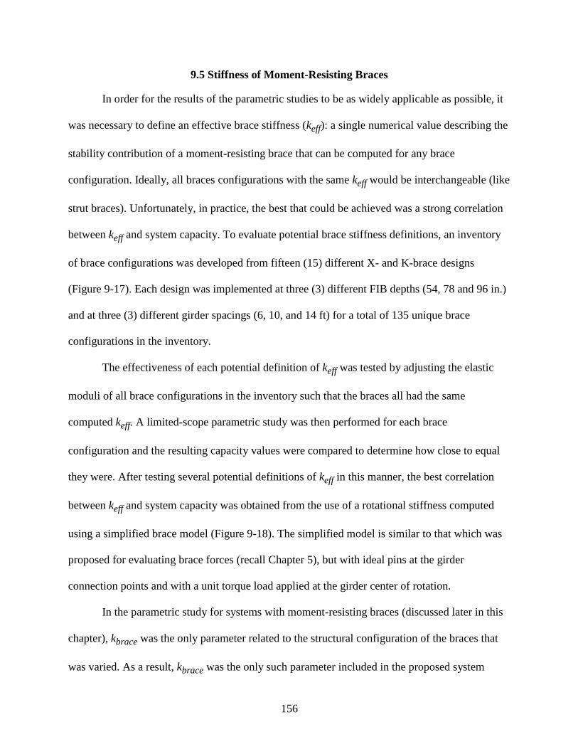
156
9.5 Stiffness of Moment-Resisting Braces
In order for the results of the parametric studies to be as widely applicable as possible, it
was necessary to define an effective brace stiffness (keff): a single numerical value describing the
stability contribution of a moment-resisting brace that can be computed for any brace
configuration. Ideally, all braces configurations with the same keff would be interchangeable (like
strut braces). Unfortunately, in practice, the best that could be achieved was a strong correlation
between keff and system capacity. To evaluate potential brace stiffness definitions, an inventory
of brace configurations was developed from fifteen (15) different X- and K-brace designs
(Figure 9-17). Each design was implemented at three (3) different FIB depths (54, 78 and 96 in.)
and at three (3) different girder spacings (6, 10, and 14 ft) for a total of 135 unique brace
configurations in the inventory.
The effectiveness of each potential definition of keff was tested by adjusting the elastic
moduli of all brace configurations in the inventory such that the braces all had the same
computed keff. A limited-scope parametric study was then performed for each brace
configuration and the resulting capacity values were compared to determine how close to equal
they were. After testing several potential definitions of keff in this manner, the best correlation
between keff and system capacity was obtained from the use of a rotational stiffness computed
using a simplified brace model (Figure 9-18). The simplified model is similar to that which was
proposed for evaluating brace forces (recall Chapter 5), but with ideal pins at the girder
connection points and with a unit torque load applied at the girder center of rotation.
In the parametric study for systems with moment-resisting braces (discussed later in this
chapter), kbrace was the only parameter related to the structural configuration of the braces that
was varied. As a result, kbrace was the only such parameter included in the proposed system
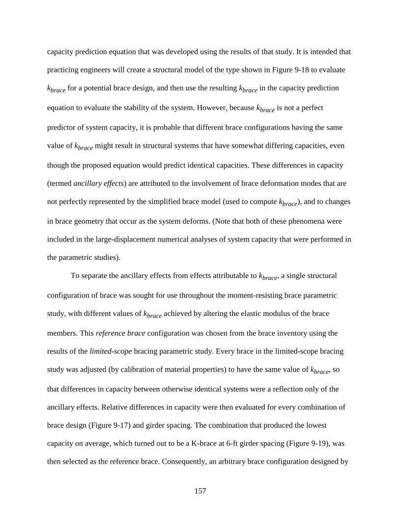
157
capacity prediction equation that was developed using the results of that study. It is intended that
practicing engineers will create a structural model of the type shown in Figure 9-18 to evaluate
kbrace for a potential brace design, and then use the resulting kbrace in the capacity prediction
equation to evaluate the stability of the system. However, because kbrace is not a perfect
predictor of system capacity, it is probable that different brace configurations having the same
value of kbrace might result in structural systems that have somewhat differing capacities, even
though the proposed equation would predict identical capacities. These differences in capacity
(termed ancillary effects) are attributed to the involvement of brace deformation modes that are
not perfectly represented by the simplified brace model (used to compute kbrace), and to changes
in brace geometry that occur as the system deforms. (Note that both of these phenomena were
included in the large-displacement numerical analyses of system capacity that were performed in
the parametric studies).
To separate the ancillary effects from effects attributable to kbrace, a single structural
configuration of brace was sought for use throughout the moment-resisting brace parametric
study, with different values of kbrace achieved by altering the elastic modulus of the brace
members. This reference brace configuration was chosen from the brace inventory using the
results of the limited-scope bracing parametric study. Every brace in the limited-scope bracing
study was adjusted (by calibration of material properties) to have the same value of kbrace, so
that differences in capacity between otherwise identical systems were a reflection only of the
ancillary effects. Relative differences in capacity were then evaluated for every combination of
brace design (Figure 9-17) and girder spacing. The combination that produced the lowest
capacity on average, which turned out to be a K-brace at 6-ft girder spacing (Figure 9-19), was
then selected as the reference brace. Consequently, an arbitrary brace configuration designed by

158
a practicing engineer is likely to have ancillary effects that only increase the capacity of the
system relative to the reference brace used in this study, and the capacity of the system predicted
by the equations developed in this study is therefore likely to be conservatively low. In all
subsequent parametric studies discussed in this chapter, different values of kbrace were achieved
by altering the elastic modulus of the brace members in the reference brace shown in Figure
9-19.
9.6 Selection of Parameters for Moment-Resisting Brace Parametric Study
System parameters that were varied in the moment-resisting brace parametric study were
as follows:
FIB cross-section depth (in)
Span length (ft)
Wind pressure (psf)
Effective brace stiffness (kip-ft/rad)
Number of interior brace points
Skew angle (deg)
Seven (7) of the eight (8) standard FIB cross-sections were included in the study. (The 36″ FIB
was excluded because the cross-section (Figure 9-20) is so shallow that usage of moment-
resisting braces is unwarranted and unfeasible.) For each FIB, capacity analyses were performed
for every combination of span length, wind pressure, effective brace stiffnesses, and number of
interior brace points sampled from the values listed in Table 9-3, for a total of 17,760 analyses.
This study only considered two-girder systems because it was determined from sensitivity
studies that when moment-resisting braces are used, the two-girder system is always the least
stable phase of construction.
Span lengths, skew angles, and wind pressure values were identical to those used in the
strut brace parametric study, while the number of interior brace points varied from 0 (end bracing
only) to 3 (end bracing with quarter-point interior bracing). As in the strut brace study, the
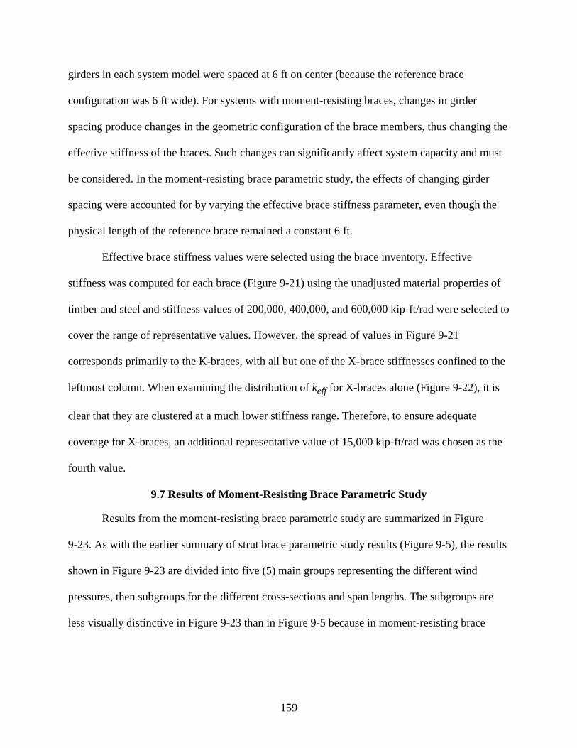
159
girders in each system model were spaced at 6 ft on center (because the reference brace
configuration was 6 ft wide). For systems with moment-resisting braces, changes in girder
spacing produce changes in the geometric configuration of the brace members, thus changing the
effective stiffness of the braces. Such changes can significantly affect system capacity and must
be considered. In the moment-resisting brace parametric study, the effects of changing girder
spacing were accounted for by varying the effective brace stiffness parameter, even though the
physical length of the reference brace remained a constant 6 ft.
Effective brace stiffness values were selected using the brace inventory. Effective
stiffness was computed for each brace (Figure 9-21) using the unadjusted material properties of
timber and steel and stiffness values of 200,000, 400,000, and 600,000 kip-ft/rad were selected to
cover the range of representative values. However, the spread of values in Figure 9-21
corresponds primarily to the K-braces, with all but one of the X-brace stiffnesses confined to the
leftmost column. When examining the distribution of keff for X-braces alone (Figure 9-22), it is
clear that they are clustered at a much lower stiffness range. Therefore, to ensure adequate
coverage for X-braces, an additional representative value of 15,000 kip-ft/rad was chosen as the
fourth value.
9.7 Results of Moment-Resisting Brace Parametric Study
Results from the moment-resisting brace parametric study are summarized in Figure
9-23. As with the earlier summary of strut brace parametric study results (Figure 9-5), the results
shown in Figure 9-23 are divided into five (5) main groups representing the different wind
pressures, then subgroups for the different cross-sections and span lengths. The subgroups are
less visually distinctive in Figure 9-23 than in Figure 9-5 because in moment-resisting brace
160
cases, the effective brace stiffness has a much greater influence on the system capacity than does
the anchor stiffness or the number of girders.
In order to develop a capacity prediction equation for moment-resisting braced systems, it
was useful to establish a baseline capacity (C0) to which correction factors could be added to
account for the effects of bracing stiffness and wind pressure. However, it would have been
illogical to include systems with zero (0) effective brace stiffness in the study, because this
would have been equivalent to simultaneously analyzing two individual (structurally
independent) girders. Instead, a system with zero effective brace stiffness was defined as being
strut-braced, so that the girders were structurally connected but no moment resistance was
provided. Therefore, data points from Figure 9-6 were included in the interpretation of the
moment-resisting brace study results, and Equation 9-2 was used as the baseline of the capacity
prediction equation.
All cases for which the capacity exceeded 10 g were excluded from consideration
because the behavior of such systems did not exhibit meaningful lateral instability. Aside from
this change, the same criteria were used in developing the capacity prediction equation as were
used for the strut-braced study: conservative capacity predictions in 95% of cases, with the
unconservative cases not in error by more than 5%.
9.7.1 System Capacity Increase from Inclusion of Moment-Resisting End Braces
Inclusion of moment-resisting braces at the girder ends increases the capacity of the
system, however, as the effective stiffness of the end braces increases, the additional stability
produced diminishes in magnitude, resulting in capacity vs. effective brace stiffness curves that
tend to plateau (Figure 9-24). It was determined that the functional form that was the closest fit
to this behavior was a rectangular hyperbola:
161
xy
x
(9-11)
where α and β are fitting parameters. To represent the increase in capacity from the baseline
value (C0), each effective brace stiffness curve (corresponding to a unique combination of FIB
depth and span length), was translated vertically so that it passed through the origin. A
rectangular hyperbola was then fitted (using regression) to each translated curve, producing an α
and a β value.
The distribution of α values in the data set exhibited no particular trends, so a constant
value of 1,000,000 (the mean value of α, rounded off) was selected. However, the β term showed
a clear dependence on span length, so an exponential regression fit (Figure 9-25) was performed,
resulting in the expression:
30620L
e
(9-12)
where L is the span length in ft. The constant value of 1,000,000 for α and Equations 9-12 and
9-11 were incorporated together to form the capacity prediction equation:
30
0
620
1,000,000
L
brace
brace
k eC C
k
(9-13)
where C is in g, kbrace is the effective moment-resisting brace stiffness in kip-ft/rad, C0 is
calculated using Equation 9-2 and is in g, and L is in ft. Equation 9-13 meets the 95% criterion
for conservative capacity prediction.
9.7.2 System Capacity Increase from Installation of Braces at Interior Points
If braces are installed at interior points (in addition to braces at the girder ends), the
additional brace stiffness increases the overall system capacity. However, the incremental
increase in system capacity that is achieved by the addition of each new interior brace

162
diminishes. For example, the additional stability provided by a midpoint brace is greater than the
additional stability provided by replacing the midpoint brace with two (2) third-point braces (all
else being equal). However, there were no clearly observable trends between the number of
interior brace points (denoted ni) and the system capacity that could be quantitatively related to
the geometric parameters the system. Therefore the effect of interior braces was accounted for by
introducing an empirically-determined scale factor, ω, into the brace stiffness term in the
capacity prediction equation:
30
0
620
1,000,000
L
brace
brace
k eC C
k
(9-14)
where C and C0 are in g, L is the span length in ft, kbrace is the effective brace stiffness in kip-
ft/rad, and ω is a dimensionless scale factor that is equal to 1 when ni is 0.
To determine appropriate values of ω for ni > 0, three subsets of the parametric study
results data were produced, corresponding to the non-zero values of ni (1, 2, and 3). The subsets
were restricted to cases where C < 3.0 g, to ensure that each subset was representative of the
types of systems pertinent to this study. For each subset, a maximum value of ω was determined
(through trial and error), such that more than 95% the capacity values predicted by Equation 9-14
were conservative. Those values of ω were then reduced by approximately the same proportion
until 95% conservatism was achieved over the full data set (Figure 9-27), including those cases
where C ≥ 3.0 g. Final ω values for use in the capacity prediction equation are listed in Table
9-4.
9.7.3 System Capacity Reduction from Inclusion of Wind Load
The process by which the effect of average wind pressure, P , on system capacity, C, was
interpreted and predicted for moment-resisting braced systems was very similar to that used for
163
the strut-braced systems (recall Section 9.4.4). As in the case of strut-braced systems, a linear
relationship (Figure 9-28) was observed for moment-resisting braced systems between the square
root of average wind pressure ( P ) and system capacity, and the corresponding slope was
defined as the wind pressure coefficient (mw). For moment-resisting braced systems in which the
effective brace stiffness was small, the relationship between C and P was not as linear as it was
in strut-braced systems, but for the sake of consistency, the assumption of linearity was
considered an acceptable approximation.
Linear regressions were performed to determine values of mw for every unique
combination of FIB depth, span length, effective brace stiffness, and number of interior brace
points (ni). The resulting values of mw were observed to vary nonlinearly with both span length
and effective brace stiffness, so a quadratic surface was fitted to both variables simultaneously,
in the form:
2 2
w brace brace bracem a L b k c L k d L e k f (9-15)
where a, b, c, d, e, and f are fitting parameters. In the resulting equation, the b parameter was
found to be negligibly small, so it was discarded and the remaining parameters were adjusted
such that system capacities were predicted conservatively in 95% of cases. The final curve fit
(Figure 9-29) was:
28 0.004 5100 900,000
1,000,000
brace brace
w
L Lk L km
(9-16)
where mw is in g/( psf ), L is the span length in ft, and kbrace is the effective brace stiffness in
kip-ft/rad.
Equation 9-16 was incorporated into Equation 9-14 to produce the final capacity
prediction equation for moment-resisting braced systems:

164
30
0
2
620
1,000,000
8 0.004 5100 900,0001,000,000
L
brace
brace
brace brace
k eC C
k
PL Lk L k
(9-17)
where C is the system capacity in g, L is the span length in ft, D is the FIB cross-section depth in
in., P is the average wind load per girder (calculated using Equation 9-7) in psf, kbrace is the is
the effective brace stiffness in kip-ft/rad, ω is determined from Table 9-4, and C0 (calculated
using Equation 9-2) is in g. As shown in the distribution of absolute prediction error (Figure
9-30), Equation 9-17 conservatively predicts the system capacity of a moment-resisting braced
system in over 95% of cases.
9.7.4 Consideration of Skew
For moment-resisting braced systems, it was found that Equation 9-17 predicted the
capacity of skewed systems with approximately the same accuracy as was achieved for
unskewed systems (Figure 9-31). Conservative capacity predictions were obtained in
approximately 92% of cases (i.e., approximately 8% of cases were unconservative). Therefore,
for the same reasons that were described in earlier in Section 9.4.5 (for strut-braced systems), no
further modifications were made to Equation 9-17 to account for the effects of bridge skew.
9.8 Incorporation of Aerodynamic Lift
In addition to horizontal wind pressure (drag), FIBs subjected to wind flow can also
experience vertical lift forces and torques. As discussed in Chapter 5, the drag coefficient (CD)
can be modified to include the structural demand associated with aerodynamic torque to form an
effective drag coefficient (CD,eff) that represents both drag and torque. However, lift cannot be
accommodated in the same manner and must be accounted for separately. Because lift acts along
the same vertical axis as gravity, it directly affects system capacity by either cancelling out
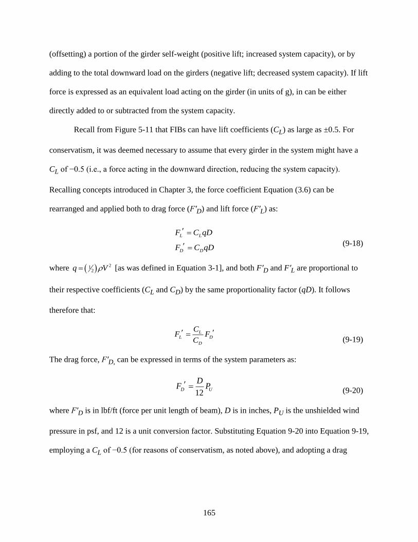
165
(offsetting) a portion of the girder self-weight (positive lift; increased system capacity), or by
adding to the total downward load on the girders (negative lift; decreased system capacity). If lift
force is expressed as an equivalent load acting on the girder (in units of g), in can be either
directly added to or subtracted from the system capacity.
Recall from Figure 5-11 that FIBs can have lift coefficients (CL) as large as ±0.5. For
conservatism, it was deemed necessary to assume that every girder in the system might have a
CL of −0.5 (i.e., a force acting in the downward direction, reducing the system capacity).
Recalling concepts introduced in Chapter 3, the force coefficient Equation (3.6) can be
rearranged and applied both to drag force (F′D) and lift force (F′L) as:
L L
D D
F C qD
F C qD
(9-18)
where 212q V [as was defined in Equation 3-1], and both F′D and F′L are proportional to
their respective coefficients (CL and CD) by the same proportionality factor (qD). It follows
therefore that:
LL D
D
CF F
C
(9-19)
The drag force, F′D, can be expressed in terms of the system parameters as:
12D U
DF P
(9-20)
where F′D is in lbf/ft (force per unit length of beam), D is in inches, PU is the unshielded wind
pressure in psf, and 12 is a unit conversion factor. Substituting Equation 9-20 into Equation 9-19,
employing a CL of −0.5 (for reasons of conservatism, as noted above), and adopting a drag
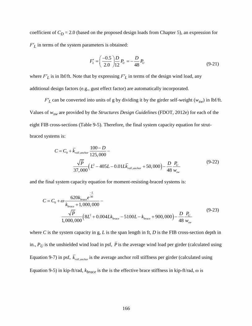
166
coefficient of CD = 2.0 (based on the proposed design loads from Chapter 5), an expression for
F′L in terms of the system parameters is obtained:
0.5
2.0 12 48L U U
D DF P P
(9-21)
where F′L is in lbf/ft. Note that by expressing F′L in terms of the design wind load, any
additional design factors (e.g., gust effect factor) are automatically incorporated.
F′L can be converted into units of g by dividing it by the girder self-weight (wsw) in lbf/ft.
Values of wsw are provided by the Structures Design Guidelines (FDOT, 2012e) for each of the
eight FIB cross-sections (Table 9-5). Therefore, the final system capacity equation for strut-
braced systems is:
0 ,
2
,
100
125,000
405 0.01 50,00037,000 48
roll anchor
Uroll anchor
sw
DC C k
PP DL L Lk
w
(9-22)
and the final system capacity equation for moment-resisting-braced systems is:
30
0
2
620
1,000,000
8 0.004 5100 900,0001,000,000 48
L
brace
brace
Ubrace brace
sw
k eC C
k
PP DL Lk L k
w
(9-23)
where C is the system capacity in g, L is the span length in ft, D is the FIB cross-section depth in
in., PU is the unshielded wind load in psf, P is the average wind load per girder (calculated using
Equation 9-7) in psf, ,roll anchork is the average anchor roll stiffness per girder (calculated using
Equation 9-5) in kip-ft/rad, kbrace is the is the effective brace stiffness in kip-ft/rad, ω is

167
determined from Table 9-4, wsw is the girder self-weight in lbf/ft (from Table 9-5), and C0
(calculated using Equation 9-2) is in g.
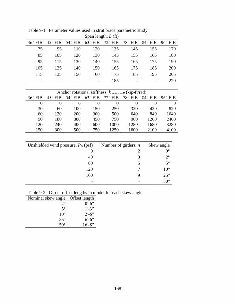
168
Table 9-1. Parameter values used in strut brace parametric study
Span length, L (ft)
36″ FIB 45″ FIB 54″ FIB 63″ FIB 72″ FIB 78″ FIB 84″ FIB 96″ FIB
75 95 110 120 135 145 155 170
85 105 120 130 145 155 165 180
95 115 130 140 155 165 175 190
105 125 140 150 165 175 185 200
115 135 150 160 175 185 195 205
- - - - 185 - - 220
Anchor rotational stiffness, kanchor,roll (kip-ft/rad)
36″ FIB 45″ FIB 54″ FIB 63″ FIB 72″ FIB 78″ FIB 84″ FIB 96″ FIB
0 0 0 0 0 0 0 0
30 60 100 150 250 320 420 820
60 120 200 300 500 640 840 1640
90 180 300 450 750 960 1260 2460
120 240 400 600 1000 1280 1680 3280
150 300 500 750 1250 1600 2100 4100
Unshielded wind pressure, PU (psf)
Number of girders, n Skew angle
0
2 0°
40
3 2°
80
5 5°
120
7 10°
160
9 25°
- - 50°
Table 9-2. Girder offset lengths in model for each skew angle
Nominal skew angle Offset length
2° 0′-6″
5° 1′-3″
10° 2′-6″
25° 6′-6″
50° 16′-8″
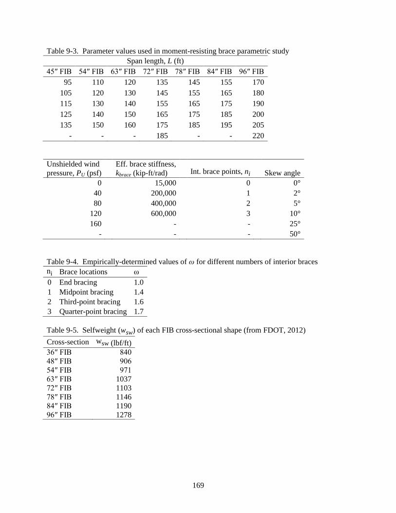
169
Table 9-3. Parameter values used in moment-resisting brace parametric study
Span length, L (ft)
45″ FIB 54″ FIB 63″ FIB 72″ FIB 78″ FIB 84″ FIB 96″ FIB
95 110 120 135 145 155 170
105 120 130 145 155 165 180
115 130 140 155 165 175 190
125 140 150 165 175 185 200
135 150 160 175 185 195 205
- - - 185 - - 220
Unshielded wind
pressure, PU (psf)
Eff. brace stiffness,
kbrace (kip-ft/rad) Int. brace points, ni Skew angle
0 15,000 0 0°
40 200,000 1 2°
80 400,000 2 5°
120 600,000 3 10°
160 - - 25°
- - - 50°
Table 9-4. Empirically-determined values of ω for different numbers of interior braces
ni Brace locations ω
0 End bracing 1.0
1 Midpoint bracing 1.4
2 Third-point bracing 1.6
3 Quarter-point bracing 1.7
Table 9-5. Selfweight (wsw) of each FIB cross-sectional shape (from FDOT, 2012)
Cross-section wsw (lbf/ft)
36″ FIB 840
48″ FIB 906
54″ FIB 971
63″ FIB 1037
72″ FIB 1103
78″ FIB 1146
84″ FIB 1190
96″ FIB 1278
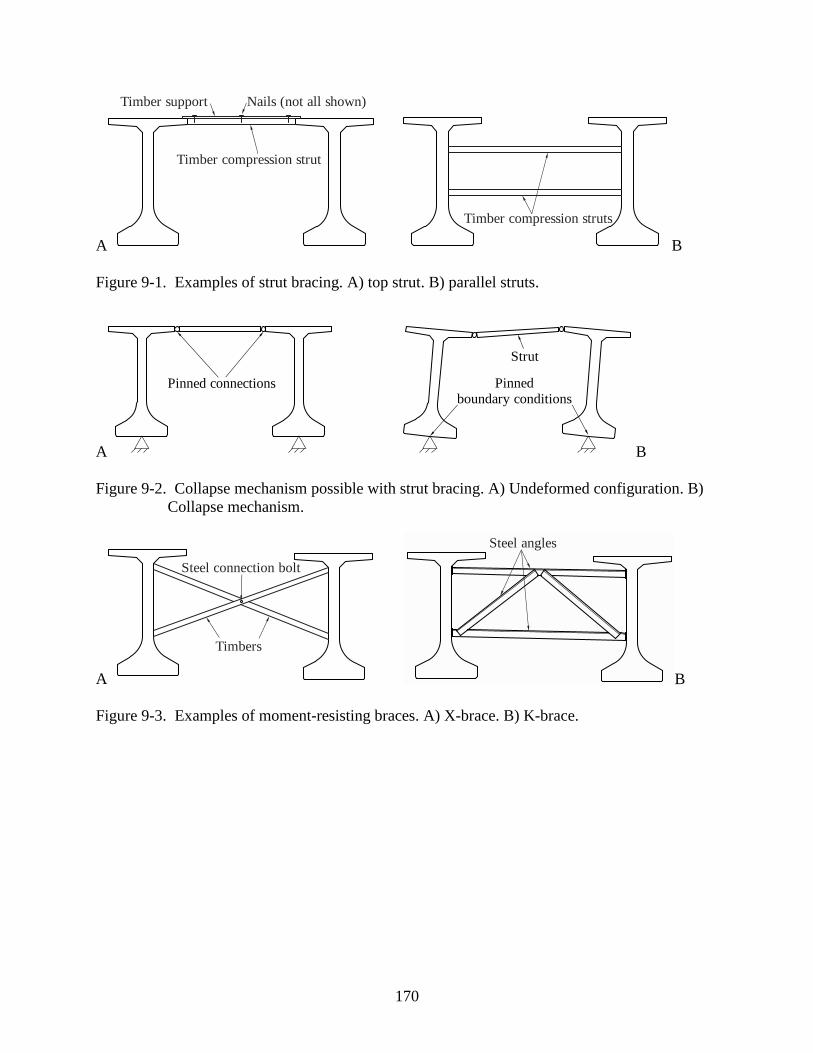
170
A
Timber compression strut
Timber support Nails (not all shown)
Timber compression struts
B
Figure 9-1. Examples of strut bracing. A) top strut. B) parallel struts.
A
Pinned connections
Pinned
boundary conditions
Strut
B
Figure 9-2. Collapse mechanism possible with strut bracing. A) Undeformed configuration. B)
Collapse mechanism.
A
Timbers
Steel connection bolt
Steel angles
B
Figure 9-3. Examples of moment-resisting braces. A) X-brace. B) K-brace.
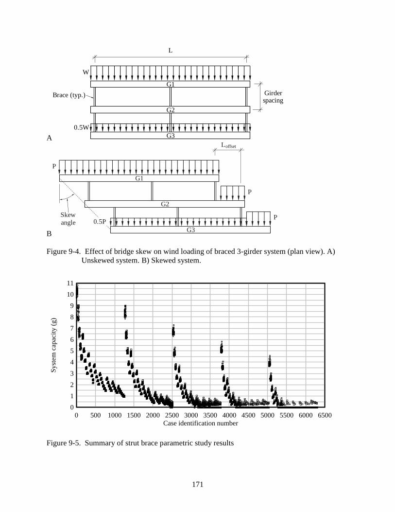
171
A
L
0.5W
W
G1
G2
G3
Brace (typ.) Girderspacing
B
0.5W
G1
G2
G3
P
P
P
Loffset
Skew
angle 0.5P
Figure 9-4. Effect of bridge skew on wind loading of braced 3-girder system (plan view). A)
Unskewed system. B) Skewed system.
Figure 9-5. Summary of strut brace parametric study results
Case identification number
Sy
stem
cap
acit
y (
g)
0 500 1000 1500 2000 2500 3000 3500 4000 4500 5000 5500 6000 6500
0
1
2
3
4
5
6
7
8
9
10
11
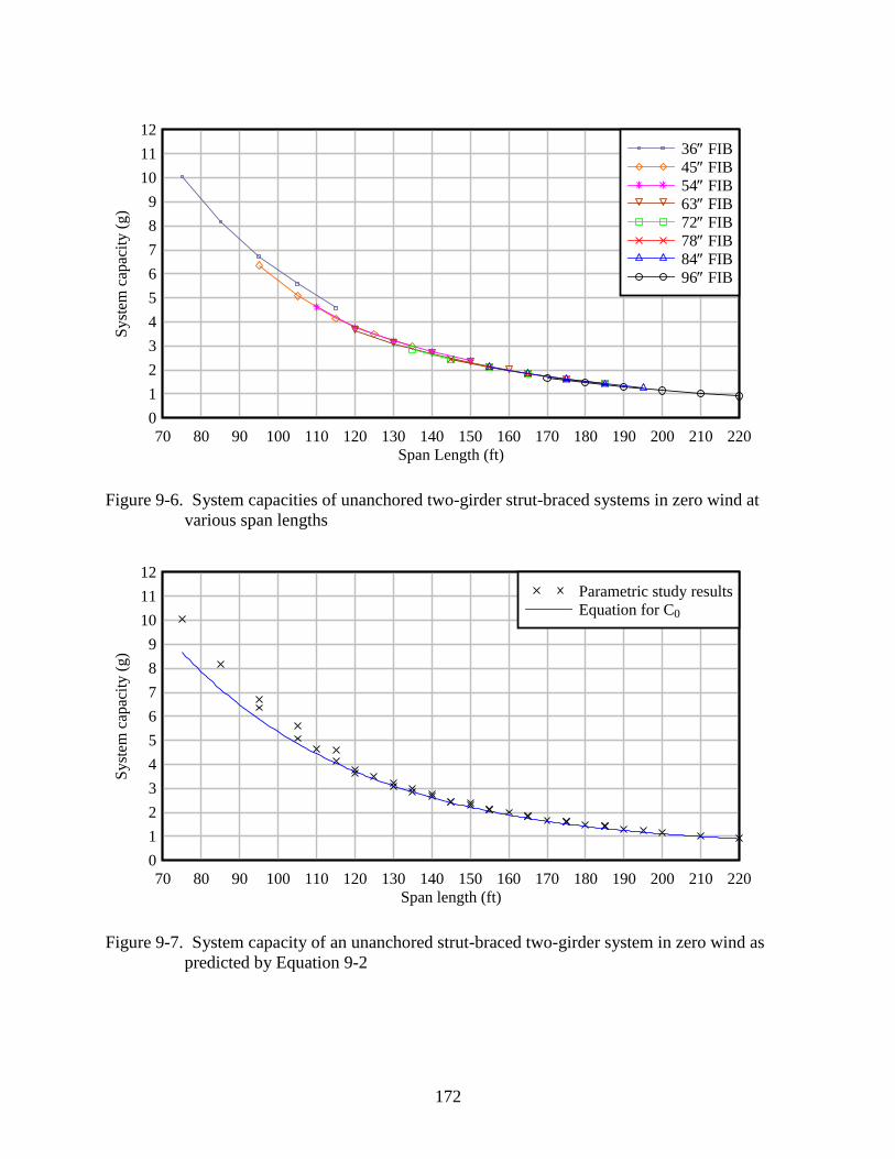
172
Figure 9-6. System capacities of unanchored two-girder strut-braced systems in zero wind at
various span lengths
Figure 9-7. System capacity of an unanchored strut-braced two-girder system in zero wind as
predicted by Equation 9-2
Span Length (ft)
Sy
stem
cap
acit
y (
g)
70 80 90 100 110 120 130 140 150 160 170 180 190 200 210 220
0
1
2
3
4
5
6
7
8
9
10
11
12
36 FIB
45 FIB
54 FIB
63 FIB
72 FIB
78 FIB
84 FIB
96 FIB
Span length (ft)
Sy
stem
cap
acit
y (
g)
70 80 90 100 110 120 130 140 150 160 170 180 190 200 210 220
0
1
2
3
4
5
6
7
8
9
10
11
12
Parametric study results
Equation for C0
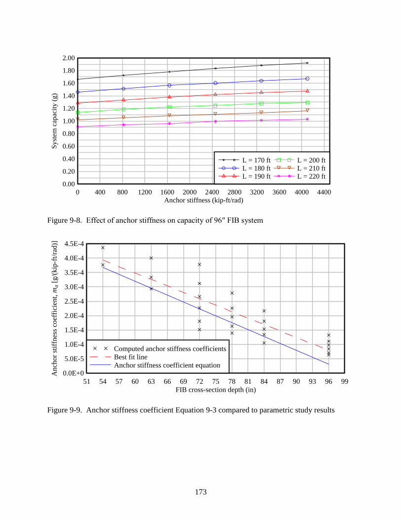
173
Figure 9-8. Effect of anchor stiffness on capacity of 96″ FIB system
Figure 9-9. Anchor stiffness coefficient Equation 9-3 compared to parametric study results
Anchor stiffness (kip-ft/rad)
Sy
stem
cap
acit
y (
g)
0 400 800 1200 1600 2000 2400 2800 3200 3600 4000 4400
0.00
0.20
0.40
0.60
0.80
1.00
1.20
1.40
1.60
1.80
2.00
L = 170 ft
L = 180 ft
L = 190 ft
L = 200 ft
L = 210 ft
L = 220 ft
FIB cross-section depth (in)
Anch
or
stif
fnes
s co
effi
cien
t, m
a [
g/(
kip
-ft/
rad)]
51 54 57 60 63 66 69 72 75 78 81 84 87 90 93 96 99
0.0E+0
5.0E-5
1.0E-4
1.5E-4
2.0E-4
2.5E-4
3.0E-4
3.5E-4
4.0E-4
4.5E-4
Computed anchor stiffness coefficients
Best fit line
Anchor stiffness coefficient equation
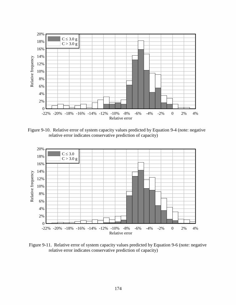
174
Figure 9-10. Relative error of system capacity values predicted by Equation 9-4 (note: negative
relative error indicates conservative prediction of capacity)
Figure 9-11. Relative error of system capacity values predicted by Equation 9-6 (note: negative
relative error indicates conservative prediction of capacity)
Relative error
Rel
ativ
e fr
equ
ency
-22% -20% -18% -16% -14% -12% -10% -8% -6% -4% -2% 0 2% 4%
0
2%
4%
6%
8%
10%
12%
14%
16%
18%
20%
C 3.0 g
C > 3.0 g
Relative error
Rel
ativ
e fr
equ
ency
-22% -20% -18% -16% -14% -12% -10% -8% -6% -4% -2% 0 2% 4%
0
2%
4%
6%
8%
10%
12%
14%
16%
18%
20%
C 3.0
C > 3.0 g
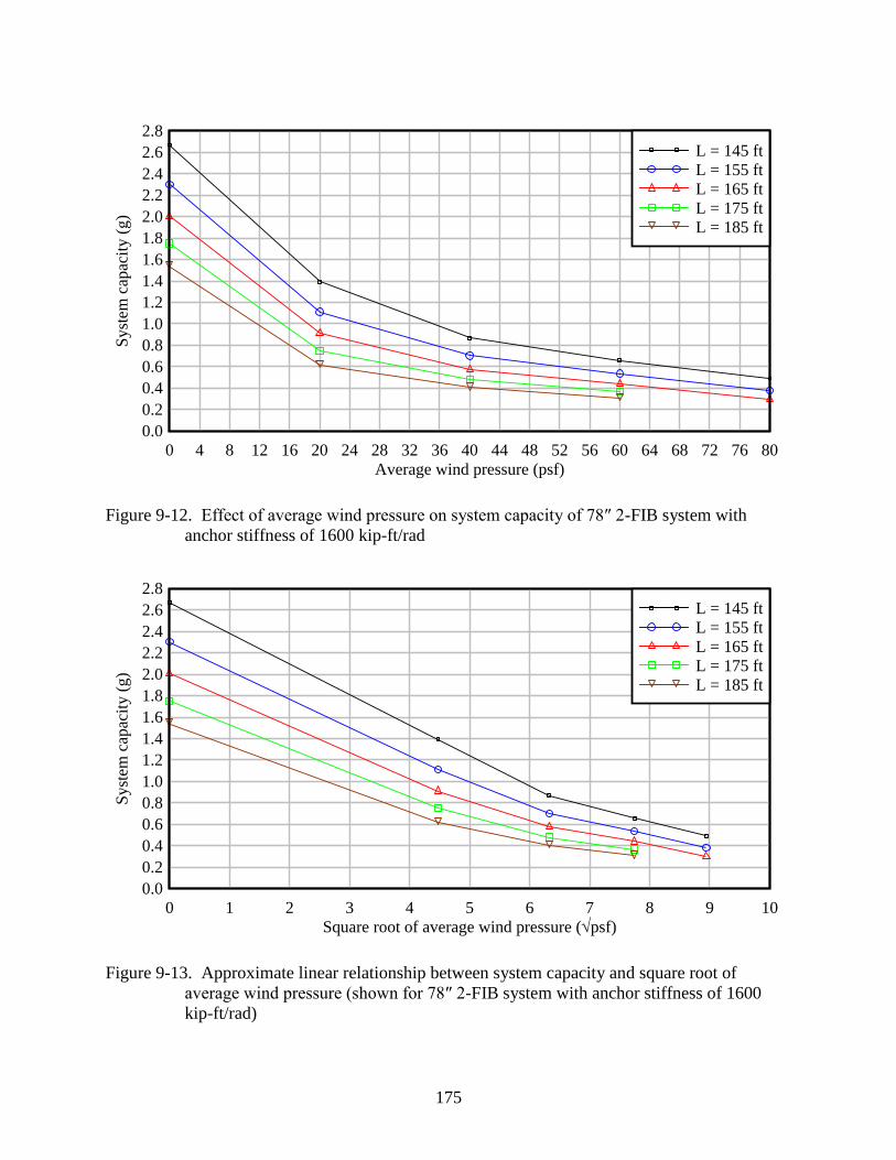
175
Figure 9-12. Effect of average wind pressure on system capacity of 78″ 2-FIB system with
anchor stiffness of 1600 kip-ft/rad
Figure 9-13. Approximate linear relationship between system capacity and square root of
average wind pressure (shown for 78″ 2-FIB system with anchor stiffness of 1600
kip-ft/rad)
Average wind pressure (psf)
Syst
em c
apac
ity (
g)
0 4 8 12 16 20 24 28 32 36 40 44 48 52 56 60 64 68 72 76 80
0.0
0.2
0.4
0.6
0.8
1.0
1.2
1.4
1.6
1.8
2.0
2.2
2.4
2.6
2.8
L = 145 ft
L = 155 ft
L = 165 ft
L = 175 ft
L = 185 ft
Square root of average wind pressure (psf)
Syst
em c
apac
ity (
g)
0 1 2 3 4 5 6 7 8 9 10
0.0
0.2
0.4
0.6
0.8
1.0
1.2
1.4
1.6
1.8
2.0
2.2
2.4
2.6
2.8
L = 145 ft
L = 155 ft
L = 165 ft
L = 175 ft
L = 185 ft
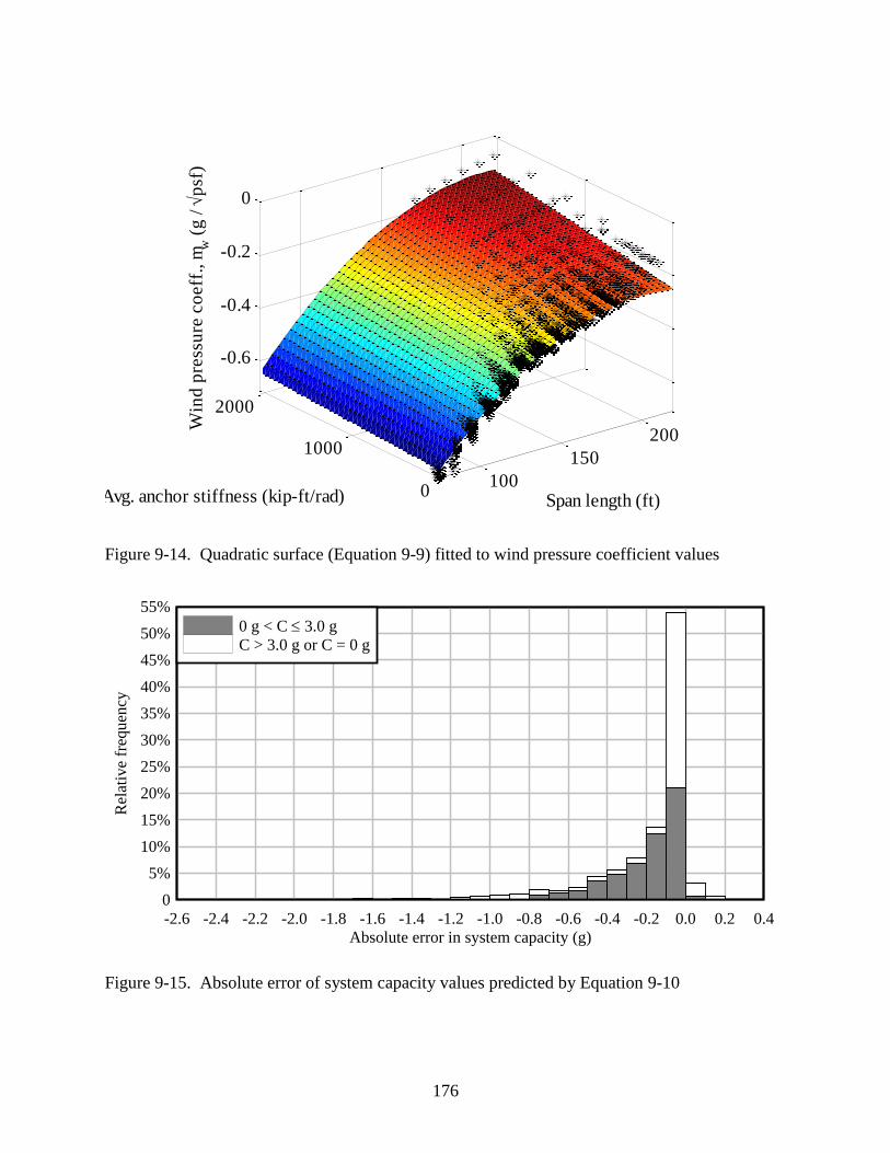
176
Figure 9-14. Quadratic surface (Equation 9-9) fitted to wind pressure coefficient values
Figure 9-15. Absolute error of system capacity values predicted by Equation 9-10
100
150
200
0
1000
2000
-0.6
-0.4
-0.2
0
Span length (ft)Avg. anchor stiffness (kip-ft/rad)
Win
d p
ress
ure
co
eff
., m
w (
g /
p
sf)
Absolute error in system capacity (g)
Rel
ativ
e fr
equ
ency
-2.6 -2.4 -2.2 -2.0 -1.8 -1.6 -1.4 -1.2 -1.0 -0.8 -0.6 -0.4 -0.2 0.0 0.2 0.4
0
5%
10%
15%
20%
25%
30%
35%
40%
45%
50%
55%
0 g < C 3.0 g
C > 3.0 g or C = 0 g
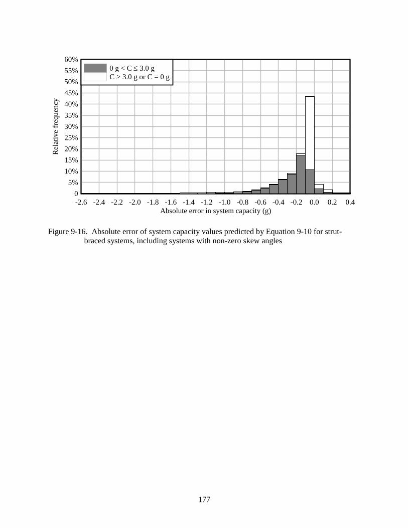
177
Figure 9-16. Absolute error of system capacity values predicted by Equation 9-10 for strut-
braced systems, including systems with non-zero skew angles
Absolute error in system capacity (g)
Rel
ativ
e fr
equ
ency
-2.6 -2.4 -2.2 -2.0 -1.8 -1.6 -1.4 -1.2 -1.0 -0.8 -0.6 -0.4 -0.2 0.0 0.2 0.4
0
5%
10%
15%
20%
25%
30%
35%
40%
45%
50%
55%
60%
0 g < C 3.0 g
C > 3.0 g or C = 0 g
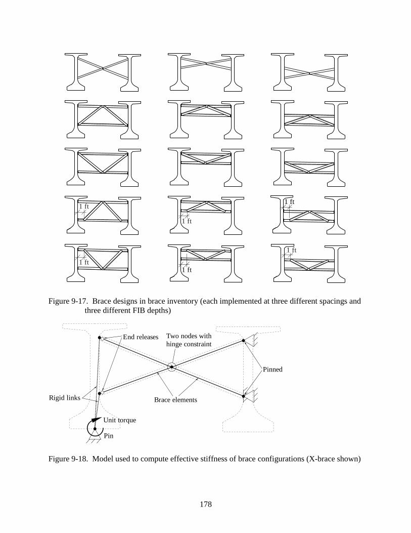
178
1 ft
1 ft
1 ft
1 ft
1 ft
1 ft
Figure 9-17. Brace designs in brace inventory (each implemented at three different spacings and
three different FIB depths)
Pin
Two nodes with
hinge constraint
Pinned
Brace elementsRigid links
End releases
Unit torque
Figure 9-18. Model used to compute effective stiffness of brace configurations (X-brace shown)
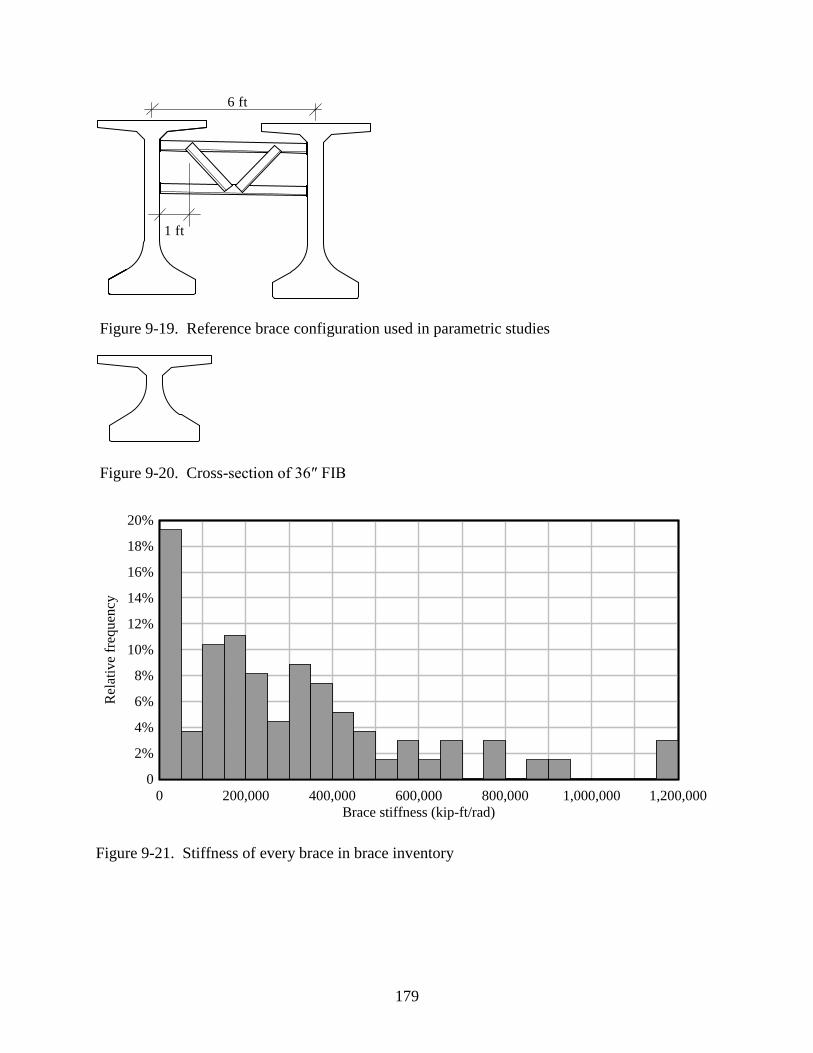
179
1 ft
6 ft
Figure 9-19. Reference brace configuration used in parametric studies
Figure 9-20. Cross-section of 36″ FIB
Figure 9-21. Stiffness of every brace in brace inventory
Brace stiffness (kip-ft/rad)
Rel
ativ
e fr
equen
cy
0 200,000 400,000 600,000 800,000 1,000,000 1,200,000
0
2%
4%
6%
8%
10%
12%
14%
16%
18%
20%
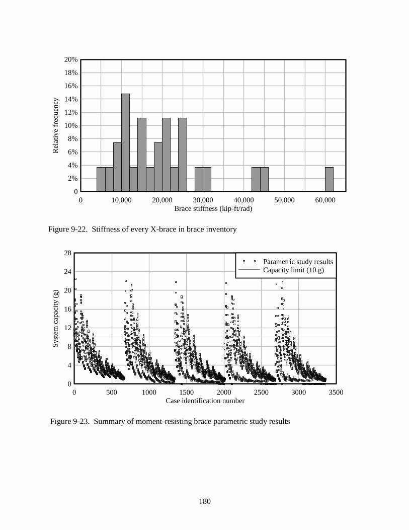
180
Figure 9-22. Stiffness of every X-brace in brace inventory
Figure 9-23. Summary of moment-resisting brace parametric study results
Brace stiffness (kip-ft/rad)
Rel
ativ
e fr
equen
cy
0 10,000 20,000 30,000 40,000 50,000 60,000
0
2%
4%
6%
8%
10%
12%
14%
16%
18%
20%
Case identification number
Sy
stem
cap
acit
y (
g)
0 500 1000 1500 2000 2500 3000 3500
0
4
8
12
16
20
24
28
Parametric study results
Capacity limit (10 g)
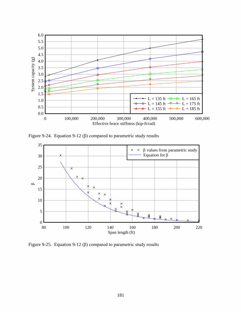
181
Figure 9-24. Equation 9-12 (β) compared to parametric study results
Figure 9-25. Equation 9-12 (β) compared to parametric study results
Effective brace stiffness (kip-ft/rad)
Sy
stem
cap
acit
y (
g)
0 100,000 200,000 300,000 400,000 500,000 600,000
0.0
0.5
1.0
1.5
2.0
2.5
3.0
3.5
4.0
4.5
5.0
5.5
6.0
L = 135 ft
L = 145 ft
L = 155 ft
L = 165 ft
L = 175 ft
L = 185 ft
Span length (ft)
80 100 120 140 160 180 200 220
0
5
10
15
20
25
30
35
values from parametric study
Equation for
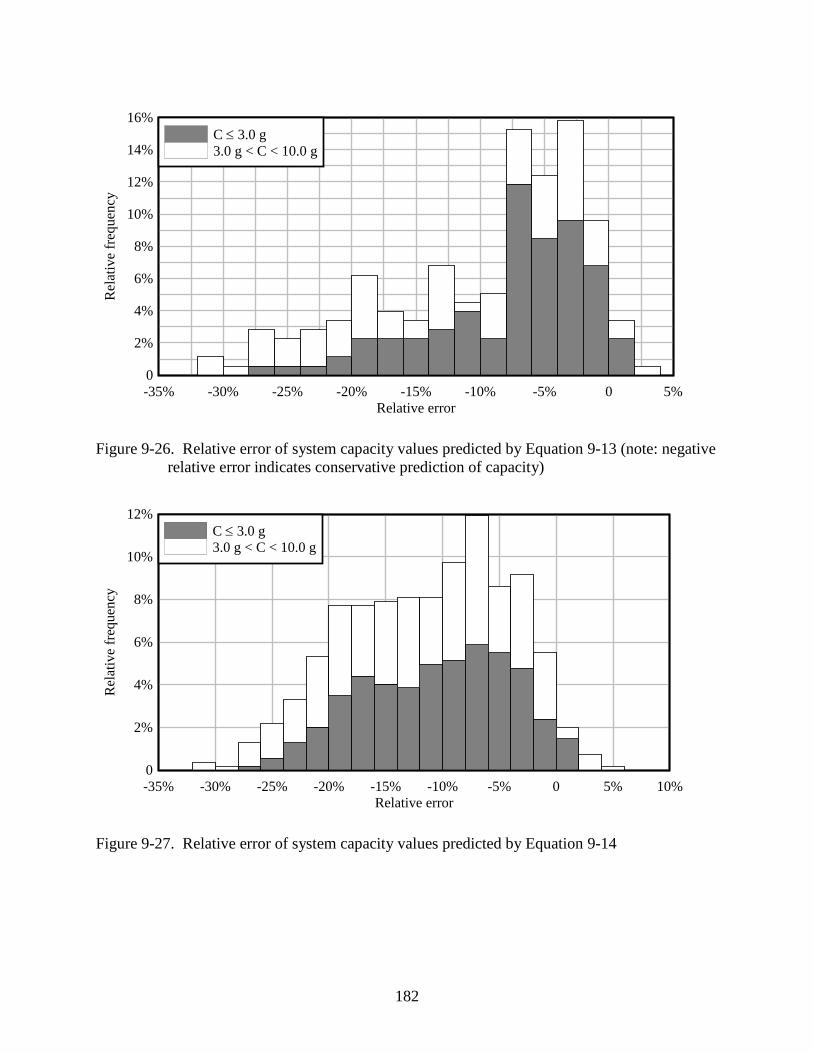
182
Figure 9-26. Relative error of system capacity values predicted by Equation 9-13 (note: negative
relative error indicates conservative prediction of capacity)
Figure 9-27. Relative error of system capacity values predicted by Equation 9-14
Relative error
Rel
ativ
e fr
equ
ency
-35% -30% -25% -20% -15% -10% -5% 0 5%
0
2%
4%
6%
8%
10%
12%
14%
16%
C 3.0 g
3.0 g < C < 10.0 g
Relative error
Rel
ativ
e fr
equ
ency
-35% -30% -25% -20% -15% -10% -5% 0 5% 10%
0
2%
4%
6%
8%
10%
12%
C 3.0 g
3.0 g < C < 10.0 g
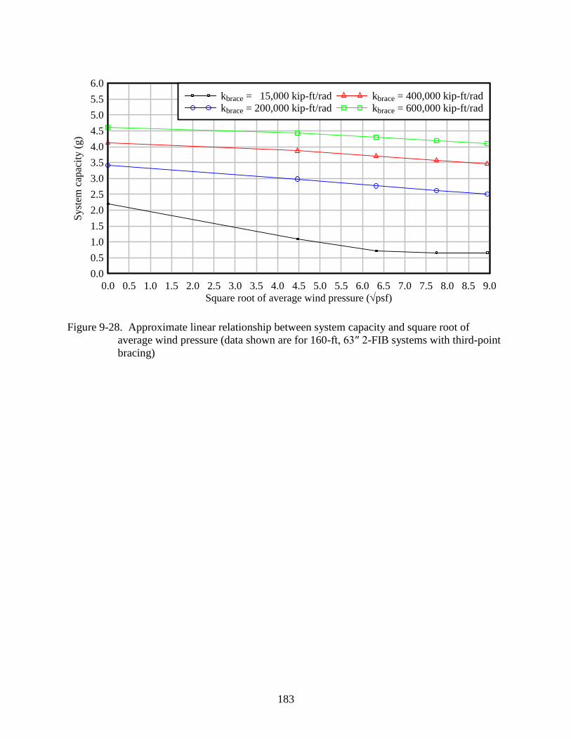
183
Figure 9-28. Approximate linear relationship between system capacity and square root of
average wind pressure (data shown are for 160-ft, 63″ 2-FIB systems with third-point
bracing)
Square root of average wind pressure (psf)
Syst
em c
apac
ity (
g)
0.0 0.5 1.0 1.5 2.0 2.5 3.0 3.5 4.0 4.5 5.0 5.5 6.0 6.5 7.0 7.5 8.0 8.5 9.0
0.0
0.5
1.0
1.5
2.0
2.5
3.0
3.5
4.0
4.5
5.0
5.5
6.0
kbrace = 015,000 kip-ft/rad
kbrace = 200,000 kip-ft/rad
kbrace = 400,000 kip-ft/rad
kbrace = 600,000 kip-ft/rad
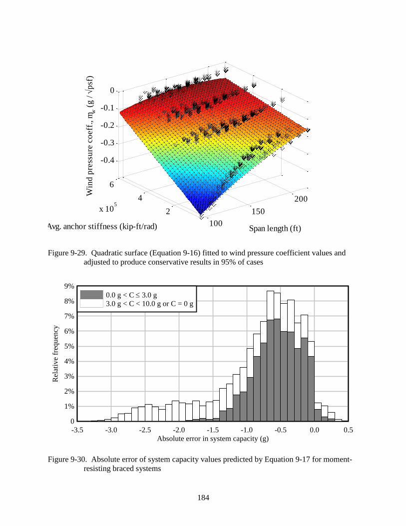
184
Figure 9-29. Quadratic surface (Equation 9-16) fitted to wind pressure coefficient values and
adjusted to produce conservative results in 95% of cases
Figure 9-30. Absolute error of system capacity values predicted by Equation 9-17 for moment-
resisting braced systems
100
150
200
2
4
6
x 105
-0.4
-0.3
-0.2
-0.1
0
Span length (ft)Avg. anchor stiffness (kip-ft/rad)
Win
d p
ress
ure
co
eff
., m
w (
g /
p
sf)
Absolute error in system capacity (g)
Rel
ativ
e fr
equen
cy
-3.5 -3.0 -2.5 -2.0 -1.5 -1.0 -0.5 0.0 0.5
0
1%
2%
3%
4%
5%
6%
7%
8%
9%
0.0 g < C 3.0 g
3.0 g < C < 10.0 g or C = 0 g
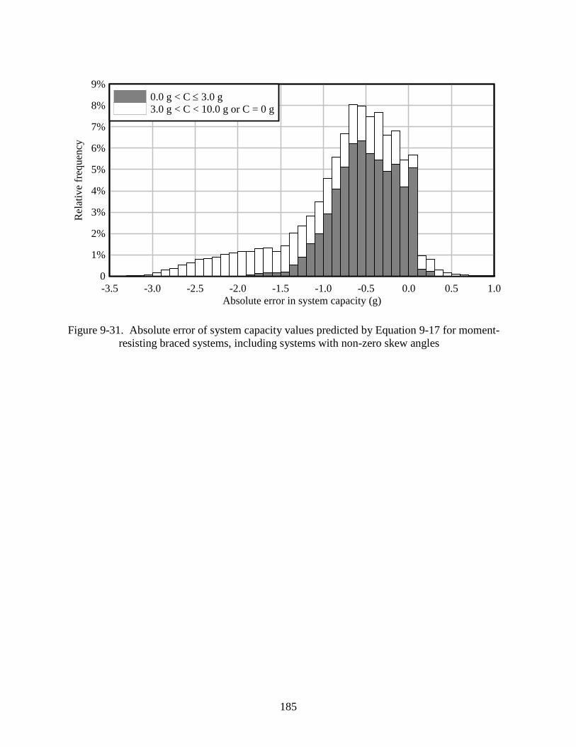
185
Figure 9-31. Absolute error of system capacity values predicted by Equation 9-17 for moment-
resisting braced systems, including systems with non-zero skew angles
Absolute error in system capacity (g)
Rel
ativ
e fr
equen
cy
-3.5 -3.0 -2.5 -2.0 -1.5 -1.0 -0.5 0.0 0.5 1.0
0
1%
2%
3%
4%
5%
6%
7%
8%
9%
0.0 g < C 3.0 g
3.0 g < C < 10.0 g or C = 0 g
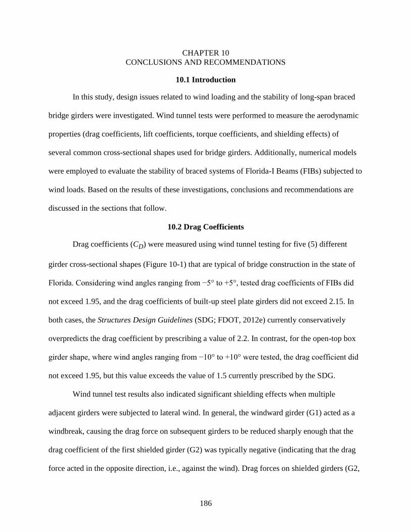
186
CHAPTER 10
CONCLUSIONS AND RECOMMENDATIONS
10.1 Introduction
In this study, design issues related to wind loading and the stability of long-span braced
bridge girders were investigated. Wind tunnel tests were performed to measure the aerodynamic
properties (drag coefficients, lift coefficients, torque coefficients, and shielding effects) of
several common cross-sectional shapes used for bridge girders. Additionally, numerical models
were employed to evaluate the stability of braced systems of Florida-I Beams (FIBs) subjected to
wind loads. Based on the results of these investigations, conclusions and recommendations are
discussed in the sections that follow.
10.2 Drag Coefficients
Drag coefficients (CD) were measured using wind tunnel testing for five (5) different
girder cross-sectional shapes (Figure 10-1) that are typical of bridge construction in the state of
Florida. Considering wind angles ranging from −5° to +5°, tested drag coefficients of FIBs did
not exceed 1.95, and the drag coefficients of built-up steel plate girders did not exceed 2.15. In
both cases, the Structures Design Guidelines (SDG; FDOT, 2012e) currently conservatively
overpredicts the drag coefficient by prescribing a value of 2.2. In contrast, for the open-top box
girder shape, where wind angles ranging from −10° to +10° were tested, the drag coefficient did
not exceed 1.95, but this value exceeds the value of 1.5 currently prescribed by the SDG.
Wind tunnel test results also indicated significant shielding effects when multiple
adjacent girders were subjected to lateral wind. In general, the windward girder (G1) acted as a
windbreak, causing the drag force on subsequent girders to be reduced sharply enough that the
drag coefficient of the first shielded girder (G2) was typically negative (indicating that the drag
force acted in the opposite direction, i.e., against the wind). Drag forces on shielded girders (G2,
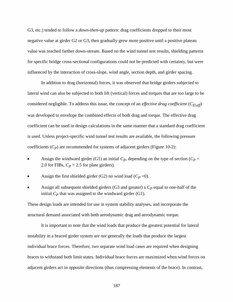
187
G3, etc.) tended to follow a down-then-up pattern: drag coefficients dropped to their most
negative value at girder G2 or G3, then gradually grew more positive until a positive plateau
value was reached farther down-stream. Based on the wind tunnel test results, shielding patterns
for specific bridge cross-sectional configurations could not be predicted with certainty, but were
influenced by the interaction of cross-slope, wind angle, section depth, and girder spacing.
In addition to drag (horizontal) forces, it was observed that bridge girders subjected to
lateral wind can also be subjected to both lift (vertical) forces and torques that are too large to be
considered negligible. To address this issue, the concept of an effective drag coefficient (CD,eff)
was developed to envelope the combined effects of both drag and torque. The effective drag
coefficient can be used in design calculations in the same manner that a standard drag coefficient
is used. Unless project-specific wind tunnel test results are available, the following pressure
coefficients (CP) are recommended for systems of adjacent girders (Figure 10-2):
Assign the windward girder (G1) an initial CP, depending on the type of section (CP =
2.0 for FIBs, CP = 2.5 for plate girders).
Assign the first shielded girder (G2) no wind load (CP =0).
Assign all subsequent shielded girders (G3 and greater) a CP equal to one-half of the
initial CP that was assigned to the windward girder (G1).
These design loads are intended for use in system stability analyses, and incorporate the
structural demand associated with both aerodynamic drag and aerodynamic torque.
It is important to note that the wind loads that produce the greatest potential for lateral
instability in a braced girder system are not generally the loads that produce the largest
individual brace forces. Therefore, two separate wind load cases are required when designing
braces to withstand both limit states. Individual brace forces are maximized when wind forces on
adjacent girders act in opposite directions (thus compressing elements of the brace). In contrast,
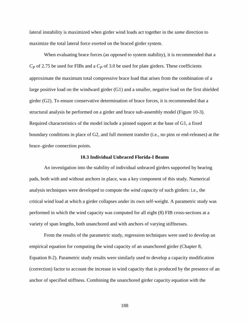
188
lateral instability is maximized when girder wind loads act together in the same direction to
maximize the total lateral force exerted on the braced girder system.
When evaluating brace forces (as opposed to system stability), it is recommended that a
CP of 2.75 be used for FIBs and a CP of 3.0 be used for plate girders. These coefficients
approximate the maximum total compressive brace load that arises from the combination of a
large positive load on the windward girder (G1) and a smaller, negative load on the first shielded
girder (G2). To ensure conservative determination of brace forces, it is recommended that a
structural analysis be performed on a girder and brace sub-assembly model (Figure 10-3).
Required characteristics of the model include a pinned support at the base of G1, a fixed
boundary conditions in place of G2, and full moment transfer (i.e., no pins or end-releases) at the
brace–girder connection points.
10.3 Individual Unbraced Florida-I Beams
An investigation into the stability of individual unbraced girders supported by bearing
pads, both with and without anchors in place, was a key component of this study. Numerical
analysis techniques were developed to compute the wind capacity of such girders: i.e., the
critical wind load at which a girder collapses under its own self-weight. A parametric study was
performed in which the wind capacity was computed for all eight (8) FIB cross-sections at a
variety of span lengths, both unanchored and with anchors of varying stiffnesses.
From the results of the parametric study, regression techniques were used to develop an
empirical equation for computing the wind capacity of an unanchored girder (Chapter 8,
Equation 8-2). Parametric study results were similarly used to develop a capacity modification
(correction) factor to account the increase in wind capacity that is produced by the presence of an
anchor of specified stiffness. Combining the unanchored girder capacity equation with the
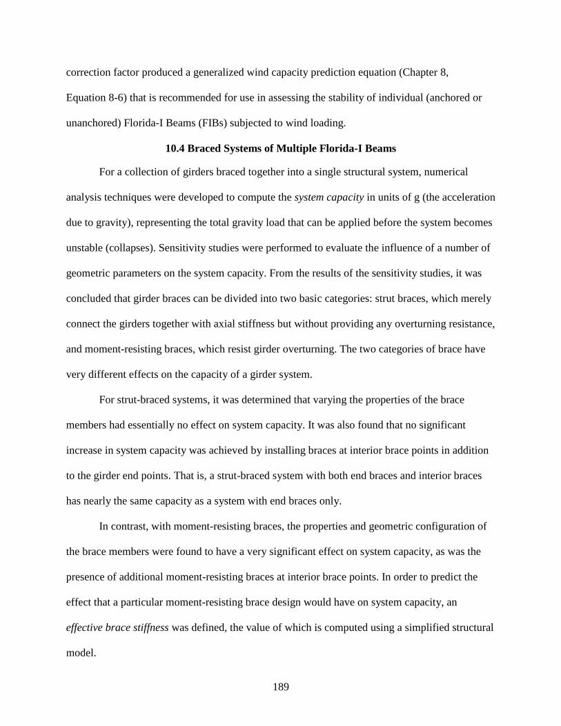
189
correction factor produced a generalized wind capacity prediction equation (Chapter 8,
Equation 8-6) that is recommended for use in assessing the stability of individual (anchored or
unanchored) Florida-I Beams (FIBs) subjected to wind loading.
10.4 Braced Systems of Multiple Florida-I Beams
For a collection of girders braced together into a single structural system, numerical
analysis techniques were developed to compute the system capacity in units of g (the acceleration
due to gravity), representing the total gravity load that can be applied before the system becomes
unstable (collapses). Sensitivity studies were performed to evaluate the influence of a number of
geometric parameters on the system capacity. From the results of the sensitivity studies, it was
concluded that girder braces can be divided into two basic categories: strut braces, which merely
connect the girders together with axial stiffness but without providing any overturning resistance,
and moment-resisting braces, which resist girder overturning. The two categories of brace have
very different effects on the capacity of a girder system.
For strut-braced systems, it was determined that varying the properties of the brace
members had essentially no effect on system capacity. It was also found that no significant
increase in system capacity was achieved by installing braces at interior brace points in addition
to the girder end points. That is, a strut-braced system with both end braces and interior braces
has nearly the same capacity as a system with end braces only.
In contrast, with moment-resisting braces, the properties and geometric configuration of
the brace members were found to have a very significant effect on system capacity, as was the
presence of additional moment-resisting braces at interior brace points. In order to predict the
effect that a particular moment-resisting brace design would have on system capacity, an
effective brace stiffness was defined, the value of which is computed using a simplified structural
model.
190
Two large-scale parametric studies were performed: one for strut-braced systems and one
for systems with moment-resisting braces. Structural parameters that were varied included the
FIB cross-section type, span length, skew angle, anchor stiffness (for strut-braced systems), and
both effective brace stiffness and number of interior brace points (for systems with moment-
resisting braces). Wind loads associated with lateral drag force, torque, and vertical uplift were
all taken into account. From the results of these parametric studies, system capacity prediction
equations were developed and recommended for use in assessing the stability of multi-girder
systems with strut braces (Chapter 9, Equation 9-22) and moment-resisting braces (Chapter 9,
Equation 9-23).
10.5 Future Research
Wind tunnel testing performed in the present study focused on individual girders and
groups of unconnected girders without any additional components present. No consideration was
given to the changes in aerodynamic properties that might occur when stay-in-place deck forms
or overhangs are present. Additionally, it was not within the scope of the wind tunnel testing
conducted in this study to quantify changes in drag force that might occur when an otherwise
shielded girder is partially exposed due to bridge skew. Hence, it may be appropriate to address
these issues with future wind tunnel testing. Alternatively, it may be possible to use a
computational fluid dynamics (CFD) analysis approach to investigate one or both of these
situations. Such an approach could potentially be validated using the wind tunnel measurements
obtained during the present study.
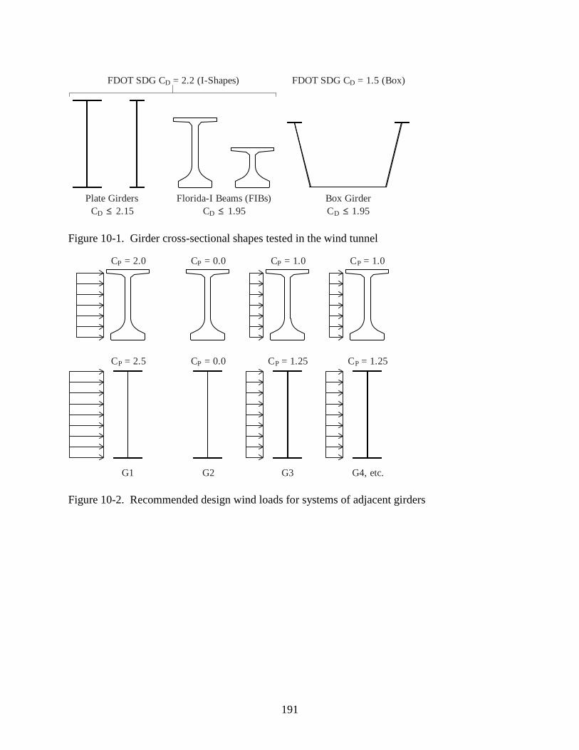
191
Box Girder
C 1.95D ≤Plate Girders
C 2.15D ≤Florida-I Beams (FIBs)
C 1.95D ≤
FDOT SDG C 2.2 (I-Shapes)D = FDOT SDG C 1.5 (Box)D =
Figure 10-1. Girder cross-sectional shapes tested in the wind tunnel
C = 2.5P
C = 2.0P
C = 0.0P
C = 0.0P
C = 1.25P
C = 1.0P
C = 1.25P
C = 1.0P
G1 G2 G3 G4, etc.
Figure 10-2. Recommended design wind loads for systems of adjacent girders
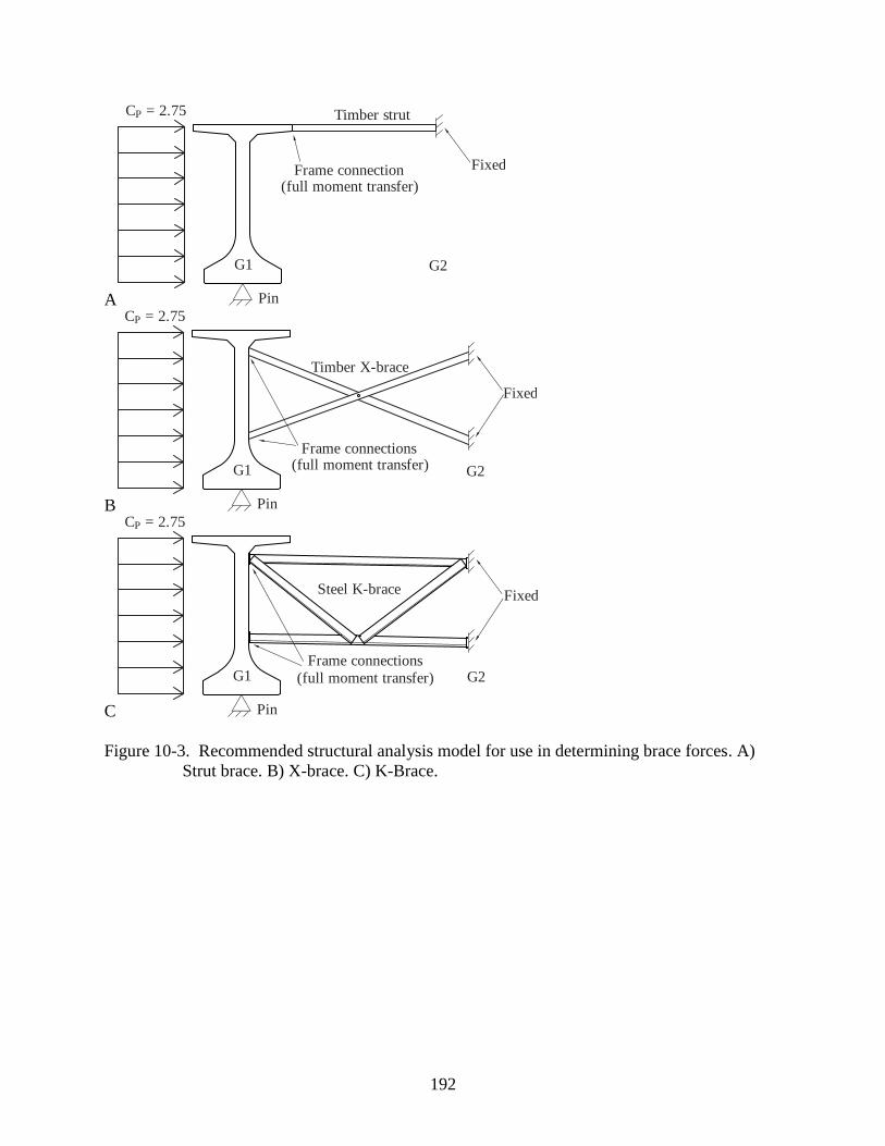
192
A
Fixed
G1 G2
Pin
Frame connection (full moment transfer)
C = 2.75P Timber strut
B
Timber X-brace
Fixed
G1 G2
Pin
Frame connections (full moment transfer)
C = 2.75P
C
G1 G2
Pin
Frame connections
(full moment transfer)
C = 2.75P
FixedSteel K-brace
Figure 10-3. Recommended structural analysis model for use in determining brace forces. A)
Strut brace. B) X-brace. C) K-Brace.

193
APPENDIX A
DIMENSIONED DRAWINGS OF WIND TUNNEL TEST CONFIGURATIONS
This appendix includes dimensioned drawings of every girder configuration that was
subjected to wind tunnel testing.
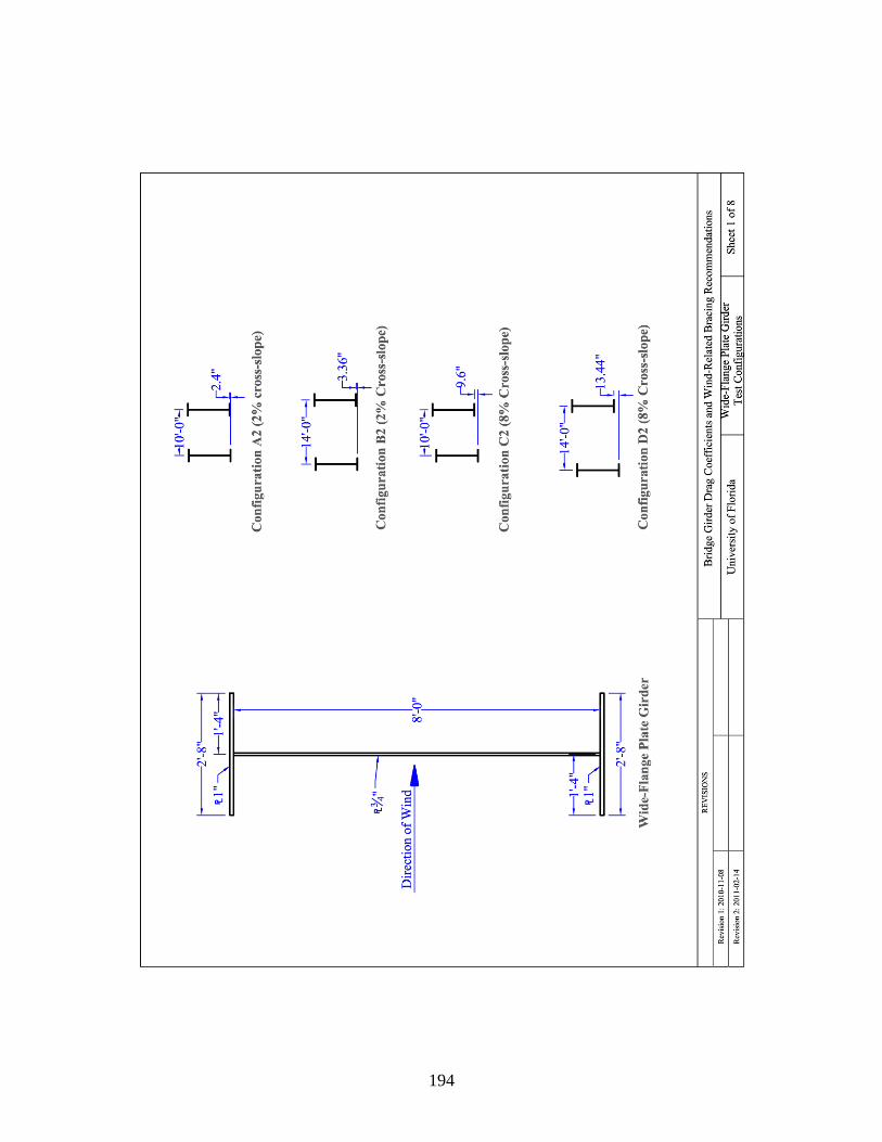
194
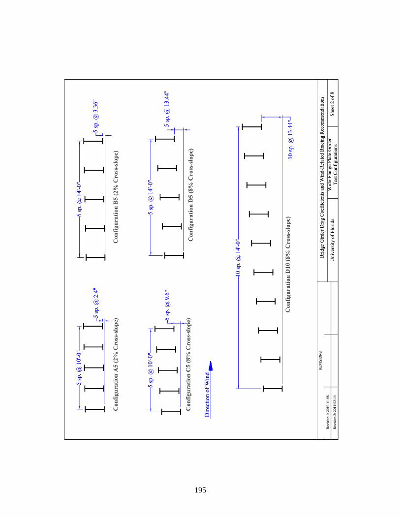
195
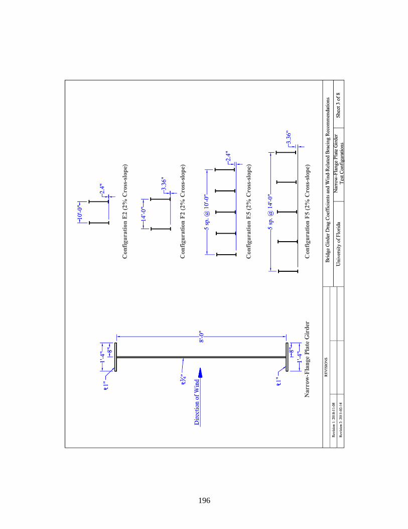
196
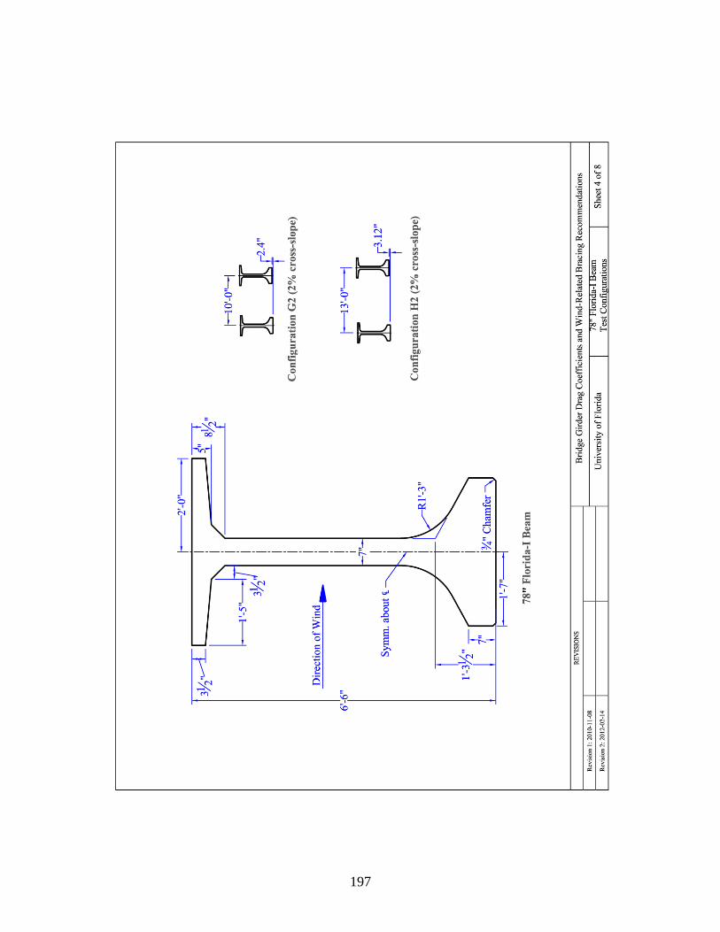
197
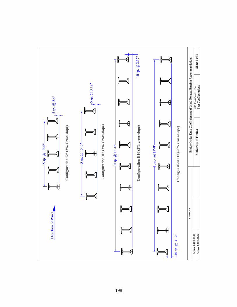
198
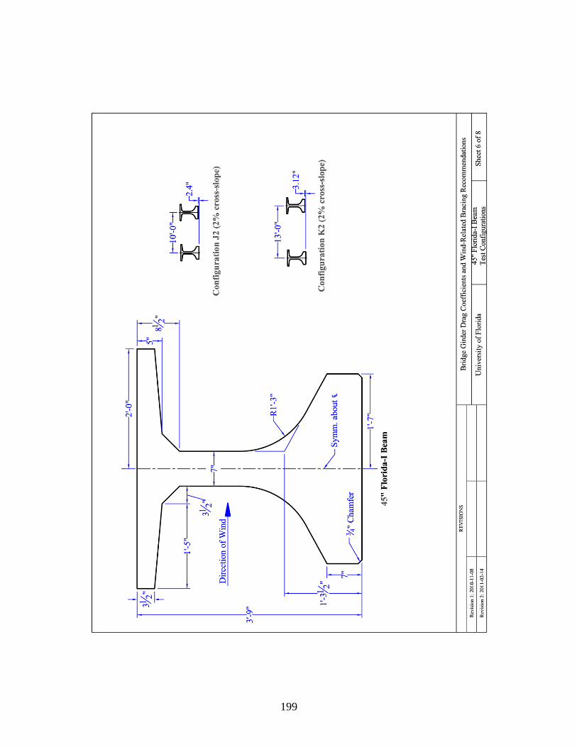
199
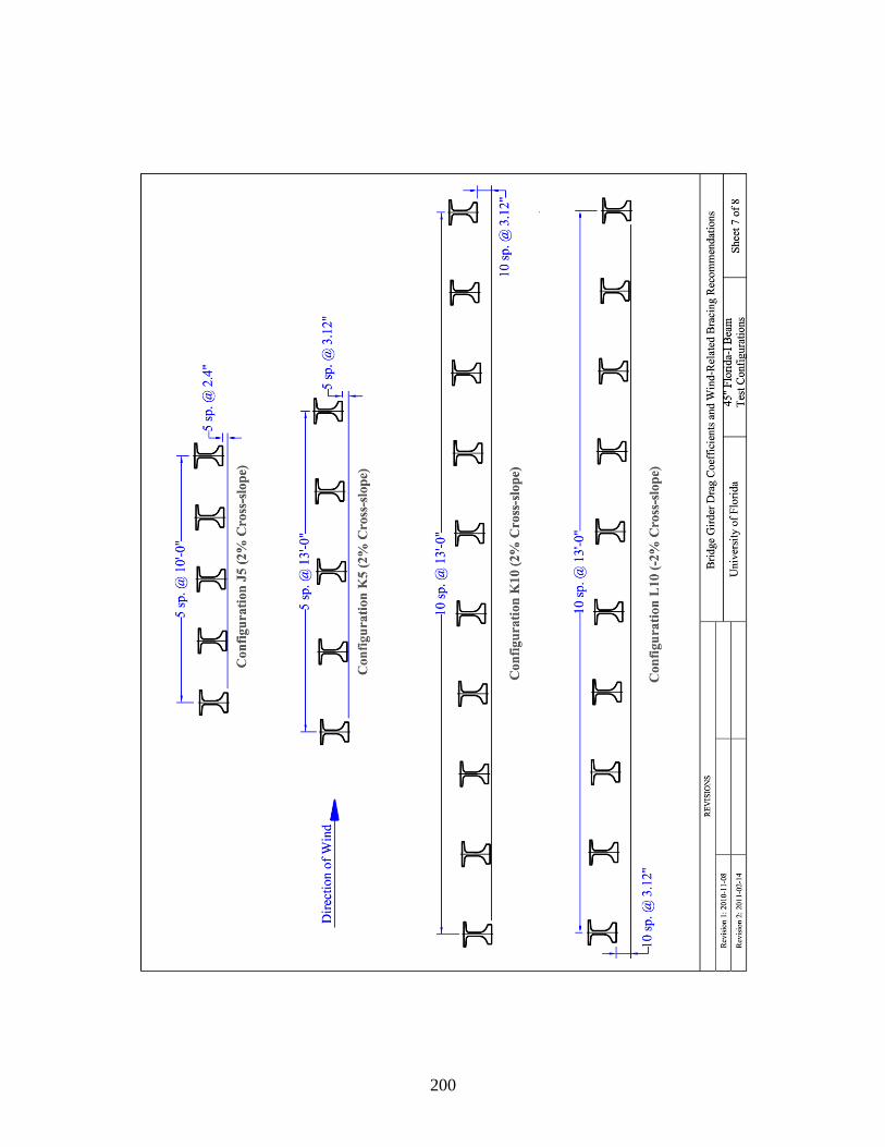
200
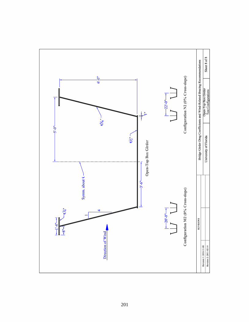
201
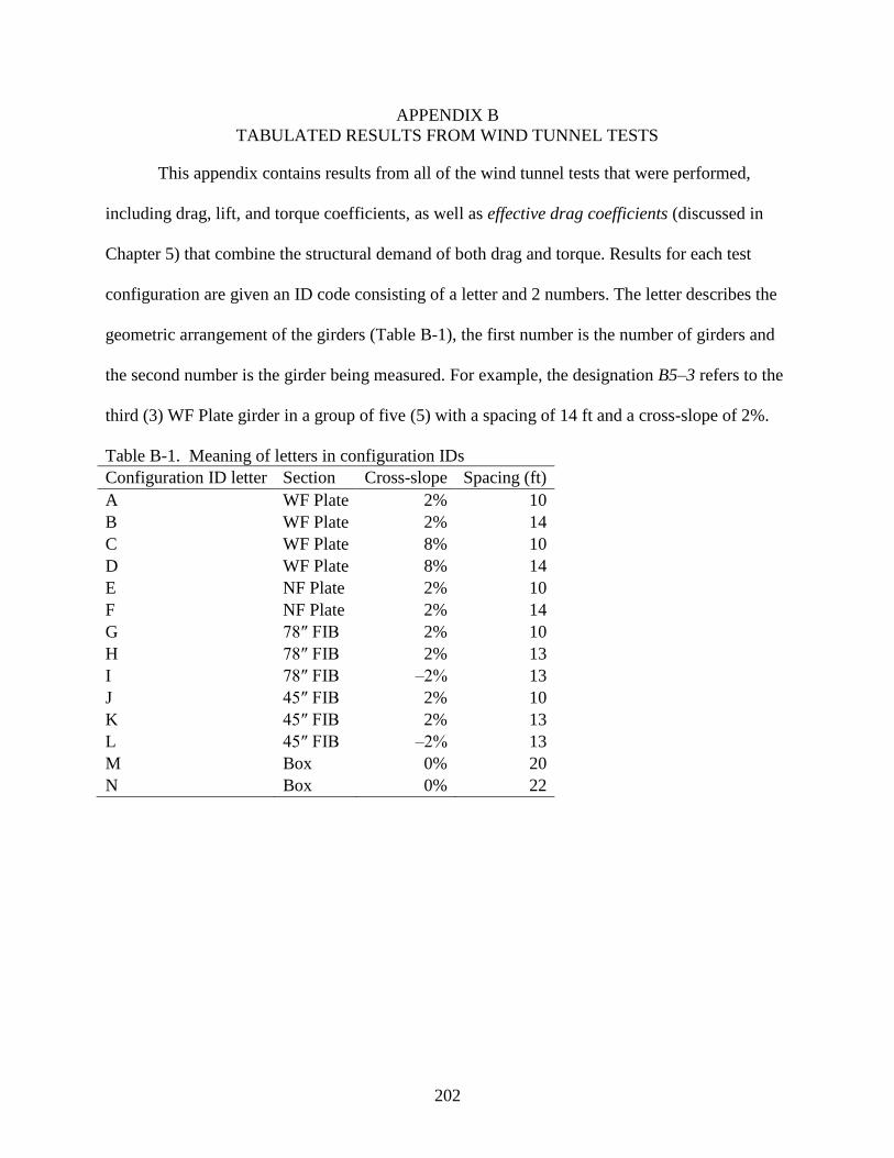
202
APPENDIX B
TABULATED RESULTS FROM WIND TUNNEL TESTS
This appendix contains results from all of the wind tunnel tests that were performed,
including drag, lift, and torque coefficients, as well as effective drag coefficients (discussed in
Chapter 5) that combine the structural demand of both drag and torque. Results for each test
configuration are given an ID code consisting of a letter and 2 numbers. The letter describes the
geometric arrangement of the girders (Table B-1), the first number is the number of girders and
the second number is the girder being measured. For example, the designation B5‒3 refers to the
third (3) WF Plate girder in a group of five (5) with a spacing of 14 ft and a cross-slope of 2%.
Table B-1. Meaning of letters in configuration IDs
Configuration ID letter Section Cross-slope Spacing (ft)
A WF Plate +2% 10
B WF Plate +2% 14
C WF Plate +8% 10
D WF Plate +8% 14
E NF Plate +2% 10
F NF Plate +2% 14
G 78″ FIB +2% 10
H 78″ FIB +2% 13
I 78″ FIB ‒2% 13
J 45″ FIB +2% 10
K 45″ FIB +2% 13
L 45″ FIB ‒2% 13
M Box +0% 20
N Box +0% 22
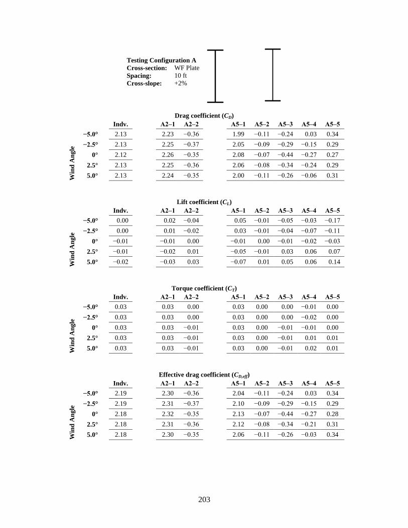
203
Testing Configuration A
Cross-section: WF Plate
Spacing: 10 ft
Cross-slope: +2%
Drag coefficient (CD)
Indv.
A2‒1 A2‒2
A5‒1 A5‒2 A5‒3 A5‒4 A5‒5
Win
d A
ng
le
−5.0°
2.13
2.23 −0.36
1.99 −0.11 −0.24 +0.03 0.34
−2.5°
2.13
2.25 −0.37
2.05 −0.09 −0.29 −0.15 0.29
+0.0°
2.12
2.26 −0.35
2.08 −0.07 −0.44 −0.27 0.27
+2.5°
2.13
2.25 −0.36
2.06 −0.08 −0.34 −0.24 0.29
+5.0°
2.13
2.24 −0.35
2.00 −0.11 −0.26 −0.06 0.31
M0‒0 M0‒0 M0‒0 M0‒0 M0‒0 M0‒0 M0‒0 M0‒0 M0‒0 M0‒0
Lift coefficient (CL)
Indv.
A2‒1 A2‒2
A5‒1 A5‒2 A5‒3 A5‒4 A5‒5
Win
d A
ng
le
−5.0°
+0.00
+0.02 −0.04
+0.05 −0.01 −0.05 −0.03 −0.17
−2.5°
+0.00
+0.01 −0.02
+0.03 −0.01 −0.04 −0.07 −0.11
+0.0°
−0.01
−0.01 +0.00
−0.01 +0.00 −0.01 −0.02 −0.03
+2.5°
−0.01
−0.02 +0.01
−0.05 −0.01 +0.03 +0.06 +0.07
+5.0°
−0.02
−0.03 +0.03
−0.07 +0.01 +0.05 +0.06 +0.14
M0‒0 M0‒0 M0‒0 M0‒0 M0‒0 M0‒0 M0‒0 M0‒0 M0‒0 M0‒0
Torque coefficient (CT)
Indv.
A2‒1 A2‒2
A5‒1 A5‒2 A5‒3 A5‒4 A5‒5
Win
d A
ng
le
−5.0°
0.03
0.03 +0.00
0.03 0.00 +0.00 −0.01 0.00
−2.5°
0.03
0.03 +0.00
0.03 0.00 +0.00 −0.02 0.00
+0.0°
0.03
0.03 −0.01
0.03 0.00 −0.01 −0.01 0.00
+2.5°
0.03
0.03 −0.01
0.03 0.00 −0.01 +0.01 0.01
+5.0°
0.03
0.03 −0.01
0.03 0.00 −0.01 +0.02 0.01
M0‒0 M0‒0 M0‒0 M0‒0 M0‒0 M0‒0 M0‒0 M0‒0 M0‒0 M0‒0
Effective drag coefficient (CD,eff)
Indv.
A2‒1 A2‒2
A5‒1 A5‒2 A5‒3 A5‒4 A5‒5
Win
d A
ng
le
−5.0°
2.19
2.30 −0.36
2.04 −0.11 −0.24 +0.03 0.34
−2.5°
2.19
2.31 −0.37
2.10 −0.09 −0.29 −0.15 0.29
+0.0°
2.18
2.32 −0.35
2.13 −0.07 −0.44 −0.27 0.28
+2.5°
2.18
2.31 −0.36
2.12 −0.08 −0.34 −0.21 0.31
+5.0°
2.18
2.30 −0.35
2.06 −0.11 −0.26 −0.03 0.34
M0‒0 M0‒0 M0‒0 M0‒0 M0‒0 M0‒0 M0‒0 M0‒0 M0‒0 M0‒0
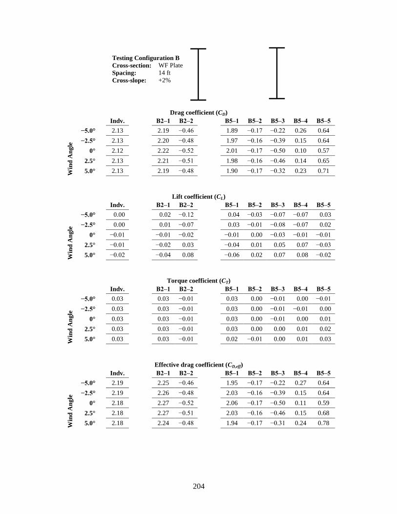
204
Testing Configuration B
Cross-section: WF Plate
Spacing: 14 ft
Cross-slope: +2%
Drag coefficient (CD)
Indv.
B2‒1 B2‒2
B5‒1 B5‒2 B5‒3 B5‒4 B5‒5
Win
d A
ng
le
−5.0°
2.13
2.19 −0.46
1.89 −0.17 −0.22 0.26 0.64
−2.5°
2.13
2.20 −0.48
1.97 −0.16 −0.39 0.15 0.64
+0.0°
2.12
2.22 −0.52
2.01 −0.17 −0.50 0.10 0.57
+2.5°
2.13
2.21 −0.51
1.98 −0.16 −0.46 0.14 0.65
+5.0°
2.13
2.19 −0.48
1.90 −0.17 −0.32 0.23 0.71
M0‒0 M0‒0 M0‒0 M0‒0 M0‒0 M0‒0 M0‒0 M0‒0 M0‒0 M0‒0
Lift coefficient (CL)
Indv.
B2‒1 B2‒2
B5‒1 B5‒2 B5‒3 B5‒4 B5‒5
Win
d A
ng
le
−5.0°
+0.00
+0.02 −0.12
+0.04 −0.03 −0.07 −0.07 +0.03
−2.5°
+0.00
+0.01 −0.07
+0.03 −0.01 −0.08 −0.07 +0.02
+0.0°
−0.01
−0.01 −0.02
−0.01 +0.00 −0.03 −0.01 −0.01
+2.5°
−0.01
−0.02 +0.03
−0.04 +0.01 +0.05 +0.07 −0.03
+5.0°
−0.02
−0.04 +0.08
−0.06 +0.02 +0.07 +0.08 −0.02
M0‒0 M0‒0 M0‒0 M0‒0 M0‒0 M0‒0 M0‒0 M0‒0 M0‒0 M0‒0
Torque coefficient (CT)
Indv.
B2‒1 B2‒2
B5‒1 B5‒2 B5‒3 B5‒4 B5‒5
Win
d A
ng
le
−5.0°
0.03
0.03 −0.01
0.03 +0.00 −0.01 +0.00 −0.01
−2.5°
0.03
0.03 −0.01
0.03 +0.00 −0.01 −0.01 +0.00
+0.0°
0.03
0.03 −0.01
0.03 +0.00 −0.01 +0.00 +0.01
+2.5°
0.03
0.03 −0.01
0.03 +0.00 +0.00 +0.01 +0.02
+5.0°
0.03
0.03 −0.01
0.02 −0.01 +0.00 +0.01 +0.03
M0‒0 M0‒0 M0‒0 M0‒0 M0‒0 M0‒0 M0‒0 M0‒0 M0‒0 M0‒0
Effective drag coefficient (CD,eff)
Indv.
B2‒1 B2‒2
B5‒1 B5‒2 B5‒3 B5‒4 B5‒5
Win
d A
ng
le
−5.0°
2.19
2.25 −0.46
1.95 −0.17 −0.22 0.27 0.64
−2.5°
2.19
2.26 −0.48
2.03 −0.16 −0.39 0.15 0.64
+0.0°
2.18
2.27 −0.52
2.06 −0.17 −0.50 0.11 0.59
+2.5°
2.18
2.27 −0.51
2.03 −0.16 −0.46 0.15 0.68
+5.0°
2.18
2.24 −0.48
1.94 −0.17 −0.31 0.24 0.78
M0‒0 M0‒0 M0‒0 M0‒0 M0‒0 M0‒0 M0‒0 M0‒0 M0‒0 M0‒0
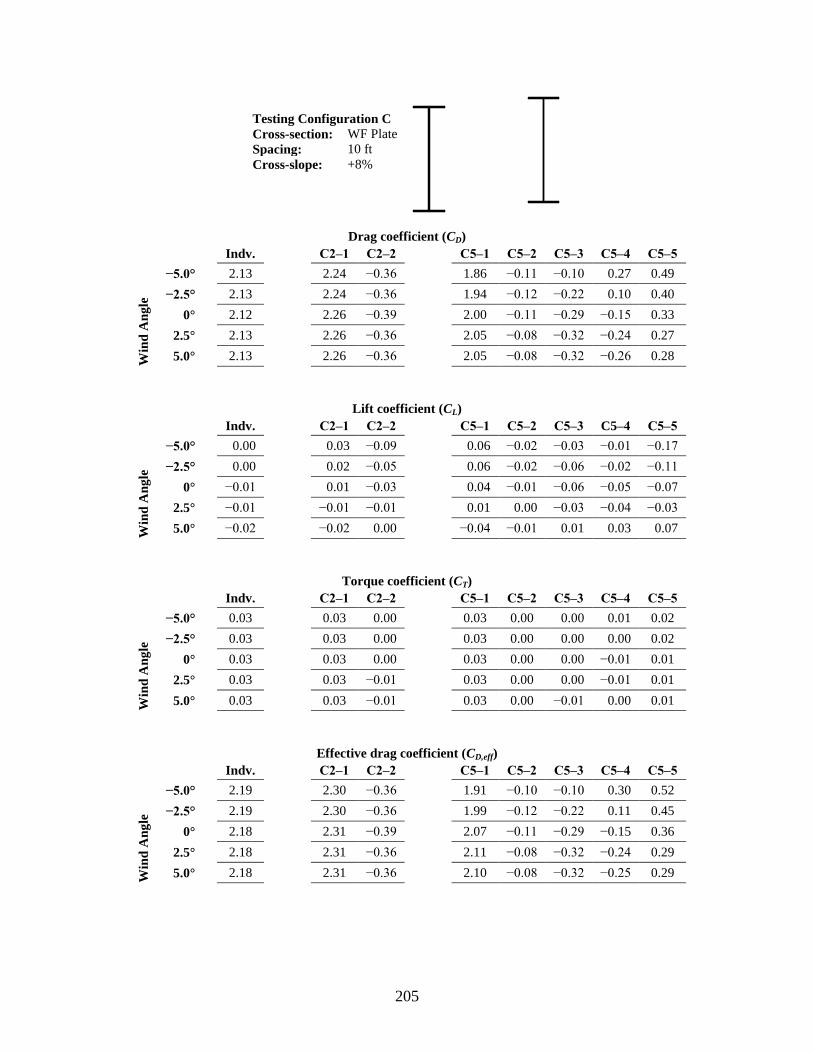
205
Testing Configuration C
Cross-section: WF Plate
Spacing: 10 ft
Cross-slope: +8%
Drag coefficient (CD)
Indv.
C2‒1 C2‒2
C5‒1 C5‒2 C5‒3 C5‒4 C5‒5
Win
d A
ng
le
−5.0°
2.13
2.24 −0.36
1.86 −0.11 −0.10 +0.27 0.49
−2.5°
2.13
2.24 −0.36
1.94 −0.12 −0.22 +0.10 0.40
+0.0°
2.12
2.26 −0.39
2.00 −0.11 −0.29 −0.15 0.33
+2.5°
2.13
2.26 −0.36
2.05 −0.08 −0.32 −0.24 0.27
+5.0°
2.13
2.26 −0.36
2.05 −0.08 −0.32 −0.26 0.28
M0‒0 M0‒0 M0‒0 M0‒0 M0‒0 M0‒0 M0‒0 M0‒0 M0‒0 M0‒0
Lift coefficient (CL)
Indv.
C2‒1 C2‒2
C5‒1 C5‒2 C5‒3 C5‒4 C5‒5
Win
d A
ng
le
−5.0°
+0.00
+0.03 −0.09
+0.06 −0.02 −0.03 −0.01 −0.17
−2.5°
+0.00
+0.02 −0.05
+0.06 −0.02 −0.06 −0.02 −0.11
+0.0°
−0.01
+0.01 −0.03
+0.04 −0.01 −0.06 −0.05 −0.07
+2.5°
−0.01
−0.01 −0.01
+0.01 +0.00 −0.03 −0.04 −0.03
+5.0°
−0.02
−0.02 +0.00
−0.04 −0.01 +0.01 +0.03 +0.07
M0‒0 M0‒0 M0‒0 M0‒0 M0‒0 M0‒0 M0‒0 M0‒0 M0‒0 M0‒0
Torque coefficient (CT)
Indv.
C2‒1 C2‒2
C5‒1 C5‒2 C5‒3 C5‒4 C5‒5
Win
d A
ng
le
−5.0°
0.03
0.03 +0.00
0.03 0.00 +0.00 +0.01 0.02
−2.5°
0.03
0.03 +0.00
0.03 0.00 +0.00 +0.00 0.02
+0.0°
0.03
0.03 +0.00
0.03 0.00 +0.00 −0.01 0.01
+2.5°
0.03
0.03 −0.01
0.03 0.00 +0.00 −0.01 0.01
+5.0°
0.03
0.03 −0.01
0.03 0.00 −0.01 +0.00 0.01
M0‒0 M0‒0 M0‒0 M0‒0 M0‒0 M0‒0 M0‒0 M0‒0 M0‒0 M0‒0
Effective drag coefficient (CD,eff)
Indv.
C2‒1 C2‒2
C5‒1 C5‒2 C5‒3 C5‒4 C5‒5
Win
d A
ng
le
−5.0°
2.19
2.30 −0.36
1.91 −0.10 −0.10 +0.30 0.52
−2.5°
2.19
2.30 −0.36
1.99 −0.12 −0.22 +0.11 0.45
+0.0°
2.18
2.31 −0.39
2.07 −0.11 −0.29 −0.15 0.36
+2.5°
2.18
2.31 −0.36
2.11 −0.08 −0.32 −0.24 0.29
+5.0°
2.18
2.31 −0.36
2.10 −0.08 −0.32 −0.25 0.29
M0‒0 M0‒0 M0‒0 M0‒0 M0‒0 M0‒0 M0‒0 M0‒0 M0‒0 M0‒0
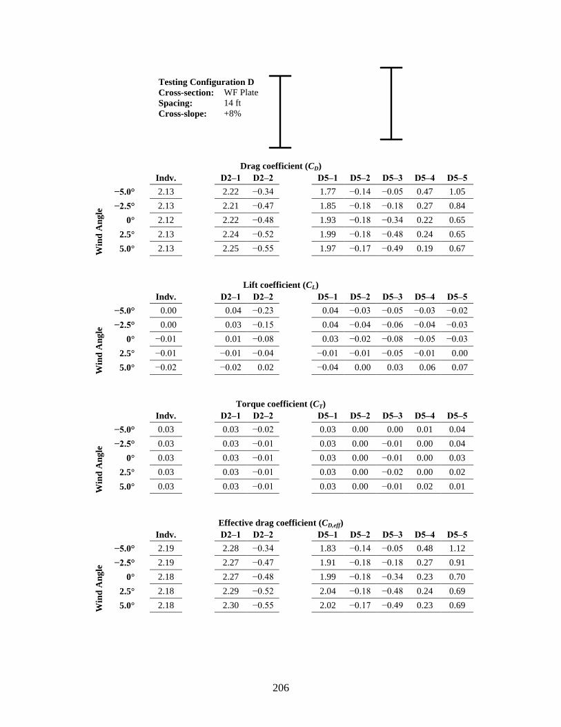
206
Testing Configuration D
Cross-section: WF Plate
Spacing: 14 ft
Cross-slope: +8%
Drag coefficient (CD)
Indv.
D2‒1 D2‒2
D5‒1 D5‒2 D5‒3 D5‒4 D5‒5
Win
d A
ng
le
−5.0°
2.13
2.22 −0.34
1.77 −0.14 −0.05 0.47 1.05
−2.5°
2.13
2.21 −0.47
1.85 −0.18 −0.18 0.27 0.84
+0.0°
2.12
2.22 −0.48
1.93 −0.18 −0.34 0.22 0.65
+2.5°
2.13
2.24 −0.52
1.99 −0.18 −0.48 0.24 0.65
+5.0°
2.13
2.25 −0.55
1.97 −0.17 −0.49 0.19 0.67
M0‒0 M0‒0 M0‒0 M0‒0 M0‒0 M0‒0 M0‒0 M0‒0 M0‒0 M0‒0
Lift coefficient (CL)
Indv.
D2‒1 D2‒2
D5‒1 D5‒2 D5‒3 D5‒4 D5‒5
Win
d A
ng
le
−5.0°
+0.00
+0.04 −0.23
+0.04 −0.03 −0.05 −0.03 −0.02
−2.5°
+0.00
+0.03 −0.15
+0.04 −0.04 −0.06 −0.04 −0.03
+0.0°
−0.01
+0.01 −0.08
+0.03 −0.02 −0.08 −0.05 −0.03
+2.5°
−0.01
−0.01 −0.04
−0.01 −0.01 −0.05 −0.01 +0.00
+5.0°
−0.02
−0.02 +0.02
−0.04 +0.00 +0.03 +0.06 +0.07
M0‒0 M0‒0 M0‒0 M0‒0 M0‒0 M0‒0 M0‒0 M0‒0 M0‒0 M0‒0
Torque coefficient (CT)
Indv.
D2‒1 D2‒2
D5‒1 D5‒2 D5‒3 D5‒4 D5‒5
Win
d A
ng
le
−5.0°
0.03
0.03 −0.02
0.03 0.00 +0.00 0.01 0.04
−2.5°
0.03
0.03 −0.01
0.03 0.00 −0.01 0.00 0.04
+0.0°
0.03
0.03 −0.01
0.03 0.00 −0.01 0.00 0.03
+2.5°
0.03
0.03 −0.01
0.03 0.00 −0.02 0.00 0.02
+5.0°
0.03
0.03 −0.01
0.03 0.00 −0.01 0.02 0.01
M0‒0 M0‒0 M0‒0 M0‒0 M0‒0 M0‒0 M0‒0 M0‒0 M0‒0 M0‒0
Effective drag coefficient (CD,eff)
Indv.
D2‒1 D2‒2
D5‒1 D5‒2 D5‒3 D5‒4 D5‒5
Win
d A
ng
le
−5.0°
2.19
2.28 −0.34
1.83 −0.14 −0.05 0.48 1.12
−2.5°
2.19
2.27 −0.47
1.91 −0.18 −0.18 0.27 0.91
+0.0°
2.18
2.27 −0.48
1.99 −0.18 −0.34 0.23 0.70
+2.5°
2.18
2.29 −0.52
2.04 −0.18 −0.48 0.24 0.69
+5.0°
2.18
2.30 −0.55
2.02 −0.17 −0.49 0.23 0.69
M0‒0 M0‒0 M0‒0 M0‒0 M0‒0 M0‒0 M0‒0 M0‒0 M0‒0 M0‒0
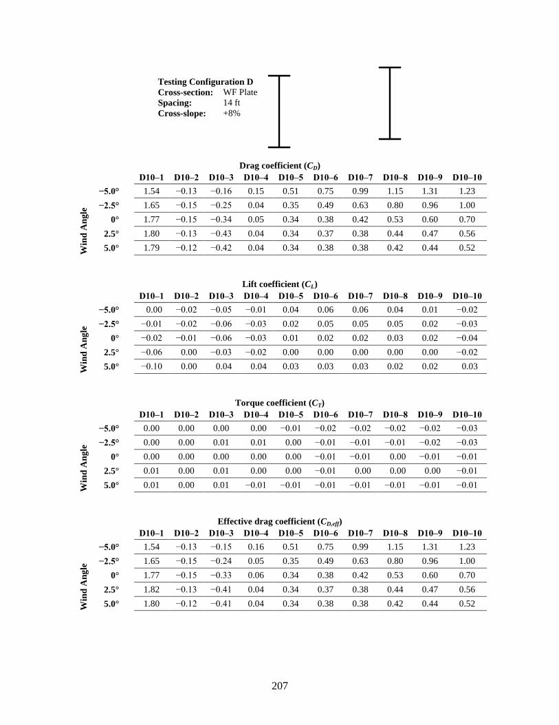
207
Testing Configuration D
Cross-section: WF Plate
Spacing: 14 ft
Cross-slope: +8%
Drag coefficient (CD)
D10‒1 D10‒2 D10‒3 D10‒4 D10‒5 D10‒6 D10‒7 D10‒8 D10‒9 D10‒10
Win
d A
ng
le
−5.0°
1.54 −0.13 −0.16 0.15 0.51 0.75 0.99 1.15 1.31 1.23
−2.5°
1.65 −0.15 −0.25 0.04 0.35 0.49 0.63 0.80 0.96 1.00
+0.0°
1.77 −0.15 −0.34 0.05 0.34 0.38 0.42 0.53 0.60 0.70
+2.5°
1.80 −0.13 −0.43 0.04 0.34 0.37 0.38 0.44 0.47 0.56
+5.0°
1.79 −0.12 −0.42 0.04 0.34 0.38 0.38 0.42 0.44 0.52
M0‒0 M0‒0 M0‒0 M0‒0 M0‒0 M0‒0 M0‒0 M0‒0 M0‒0 M0‒0
Lift coefficient (CL)
D10‒1 D10‒2 D10‒3 D10‒4 D10‒5 D10‒6 D10‒7 D10‒8 D10‒9 D10‒10
Win
d A
ng
le
−5.0°
+0.00 −0.02 −0.05 −0.01 0.04 0.06 0.06 0.04 0.01 −0.02
−2.5°
−0.01 −0.02 −0.06 −0.03 0.02 0.05 0.05 0.05 0.02 −0.03
+0.0°
−0.02 −0.01 −0.06 −0.03 0.01 0.02 0.02 0.03 0.02 −0.04
+2.5°
−0.06 +0.00 −0.03 −0.02 0.00 0.00 0.00 0.00 0.00 −0.02
+5.0°
−0.10 +0.00 +0.04 +0.04 0.03 0.03 0.03 0.02 0.02 +0.03
M0‒0 M0‒0 M0‒0 M0‒0 M0‒0 M0‒0 M0‒0 M0‒0 M0‒0 M0‒0
Torque coefficient (CT)
D10‒1 D10‒2 D10‒3 D10‒4 D10‒5 D10‒6 D10‒7 D10‒8 D10‒9 D10‒10
Win
d A
ng
le
−5.0°
0.00 0.00 0.00 +0.00 −0.01 −0.02 −0.02 −0.02 −0.02 −0.03
−2.5°
0.00 0.00 0.01 +0.01 +0.00 −0.01 −0.01 −0.01 −0.02 −0.03
+0.0°
0.00 0.00 0.00 +0.00 +0.00 −0.01 −0.01 +0.00 −0.01 −0.01
+2.5°
0.01 0.00 0.01 +0.00 +0.00 −0.01 +0.00 +0.00 +0.00 −0.01
+5.0°
0.01 0.00 0.01 −0.01 −0.01 −0.01 −0.01 −0.01 −0.01 −0.01
M0‒0 M0‒0 M0‒0 M0‒0 M0‒0 M0‒0 M0‒0 M0‒0 M0‒0 M0‒0
Effective drag coefficient (CD,eff)
D10‒1 D10‒2 D10‒3 D10‒4 D10‒5 D10‒6 D10‒7 D10‒8 D10‒9 D10‒10
Win
d A
ng
le
−5.0°
1.54 −0.13 −0.15 0.16 0.51 0.75 0.99 1.15 1.31 1.23
−2.5°
1.65 −0.15 −0.24 0.05 0.35 0.49 0.63 0.80 0.96 1.00
+0.0°
1.77 −0.15 −0.33 0.06 0.34 0.38 0.42 0.53 0.60 0.70
+2.5°
1.82 −0.13 −0.41 0.04 0.34 0.37 0.38 0.44 0.47 0.56
+5.0°
1.80 −0.12 −0.41 0.04 0.34 0.38 0.38 0.42 0.44 0.52
M0‒0 M0‒0 M0‒0 M0‒0 M0‒0 M0‒0 M0‒0 M0‒0 M0‒0 M0‒0
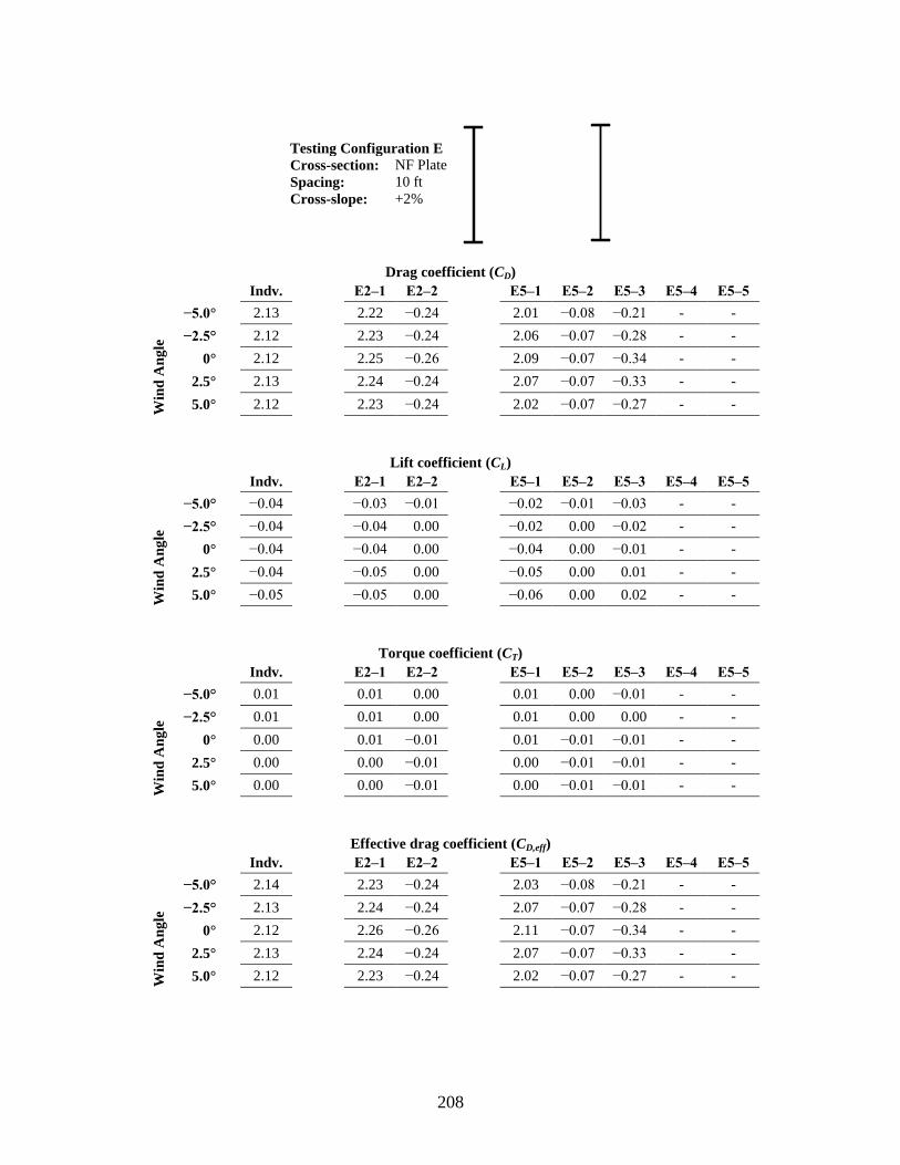
208
Testing Configuration E
Cross-section: NF Plate
Spacing: 10 ft
Cross-slope: +2%
Drag coefficient (CD)
Indv.
E2‒1 E2‒2
E5‒1 E5‒2 E5‒3 E5‒4 E5‒5
Win
d A
ng
le
−5.0°
2.13
2.22 −0.24
2.01 −0.08 −0.21 - -
−2.5°
2.12
2.23 −0.24
2.06 −0.07 −0.28 - -
+0.0°
2.12
2.25 −0.26
2.09 −0.07 −0.34 - -
+2.5°
2.13
2.24 −0.24
2.07 −0.07 −0.33 - -
+5.0°
2.12
2.23 −0.24
2.02 −0.07 −0.27 - -
M0‒0 M0‒0 M0‒0 M0‒0 M0‒0 M0‒0 M0‒0 M0‒0 M0‒0 M0‒0
Lift coefficient (CL)
Indv.
E2‒1 E2‒2
E5‒1 E5‒2 E5‒3 E5‒4 E5‒5
Win
d A
ng
le
−5.0°
−0.04
−0.03 −0.01
−0.02 −0.01 −0.03 - -
−2.5°
−0.04
−0.04 +0.00
−0.02 +0.00 −0.02 - -
+0.0°
−0.04
−0.04 +0.00
−0.04 +0.00 −0.01 - -
+2.5°
−0.04
−0.05 +0.00
−0.05 +0.00 +0.01 - -
+5.0°
−0.05
−0.05 +0.00
−0.06 +0.00 +0.02 - -
M0‒0 M0‒0 M0‒0 M0‒0 M0‒0 M0‒0 M0‒0 M0‒0 M0‒0 M0‒0
Torque coefficient (CT)
Indv.
E2‒1 E2‒2
E5‒1 E5‒2 E5‒3 E5‒4 E5‒5
Win
d A
ng
le
−5.0°
0.01
0.01 +0.00
0.01 +0.00 −0.01 - -
−2.5°
0.01
0.01 +0.00
0.01 +0.00 +0.00 - -
+0.0°
0.00
0.01 −0.01
0.01 −0.01 −0.01 - -
+2.5°
0.00
0.00 −0.01
0.00 −0.01 −0.01 - -
+5.0°
0.00
0.00 −0.01
0.00 −0.01 −0.01 - -
M0‒0 M0‒0 M0‒0 M0‒0 M0‒0 M0‒0 M0‒0 M0‒0 M0‒0 M0‒0
Effective drag coefficient (CD,eff)
Indv.
E2‒1 E2‒2
E5‒1 E5‒2 E5‒3 E5‒4 E5‒5
Win
d A
ng
le
−5.0°
2.14
2.23 −0.24
2.03 −0.08 −0.21 - -
−2.5°
2.13
2.24 −0.24
2.07 −0.07 −0.28 - -
+0.0°
2.12
2.26 −0.26
2.11 −0.07 −0.34 - -
+2.5°
2.13
2.24 −0.24
2.07 −0.07 −0.33 - -
+5.0°
2.12
2.23 −0.24
2.02 −0.07 −0.27 - -
M0‒0 M0‒0 M0‒0 M0‒0 M0‒0 M0‒0 M0‒0 M0‒0 M0‒0 M0‒0
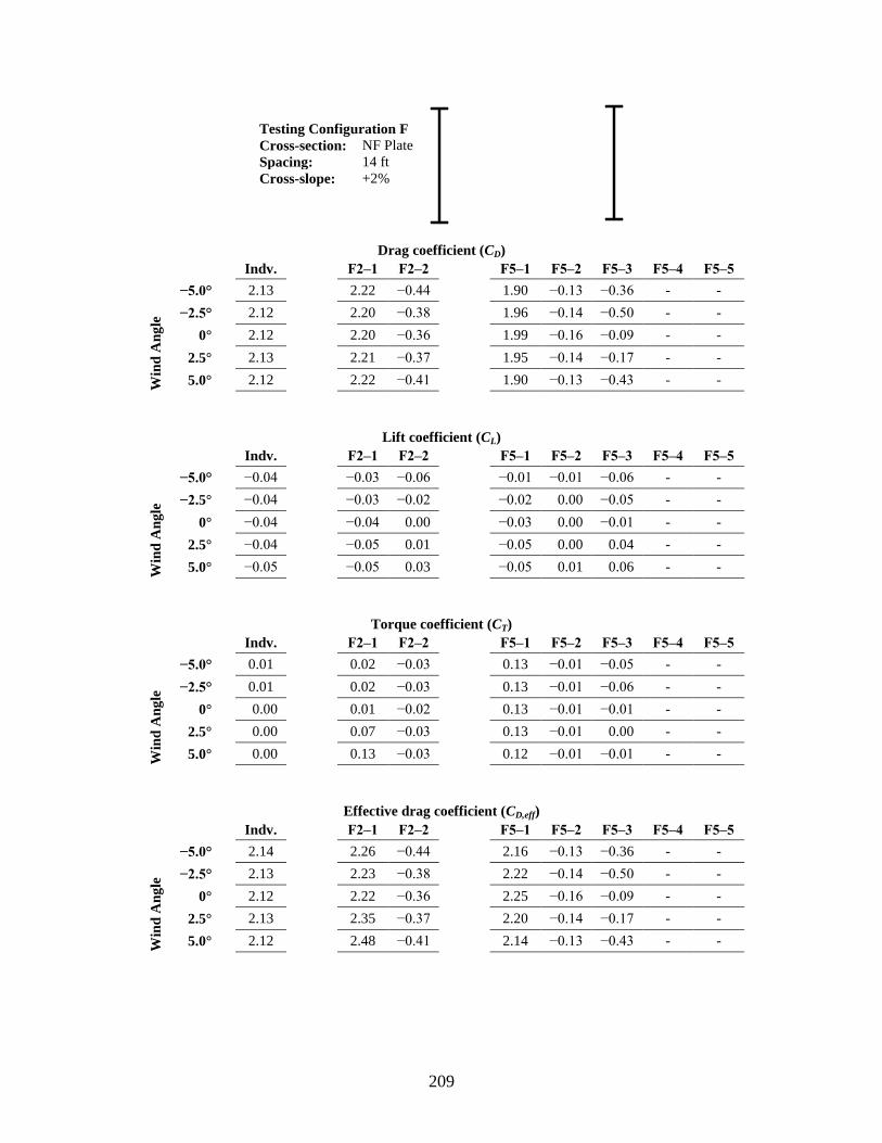
209
Testing Configuration F
Cross-section: NF Plate
Spacing: 14 ft
Cross-slope: +2%
Drag coefficient (CD)
Indv.
F2‒1 F2‒2
F5‒1 F5‒2 F5‒3 F5‒4 F5‒5
Win
d A
ng
le
−5.0°
2.13
2.22 −0.44
1.90 −0.13 −0.36 - -
−2.5°
2.12
2.20 −0.38
1.96 −0.14 −0.50 - -
+0.0°
2.12
2.20 −0.36
1.99 −0.16 −0.09 - -
+2.5°
2.13
2.21 −0.37
1.95 −0.14 −0.17 - -
+5.0°
2.12
2.22 −0.41
1.90 −0.13 −0.43 - -
M0‒0 M0‒0 M0‒0 M0‒0 M0‒0 M0‒0 M0‒0 M0‒0 M0‒0 M0‒0
Lift coefficient (CL)
Indv.
F2‒1 F2‒2
F5‒1 F5‒2 F5‒3 F5‒4 F5‒5
Win
d A
ng
le
−5.0°
−0.04
−0.03 −0.06
−0.01 −0.01 −0.06 - -
−2.5°
−0.04
−0.03 −0.02
−0.02 +0.00 −0.05 - -
+0.0°
−0.04
−0.04 +0.00
−0.03 +0.00 −0.01 - -
+2.5°
−0.04
−0.05 +0.01
−0.05 +0.00 +0.04 - -
+5.0°
−0.05
−0.05 +0.03
−0.05 +0.01 +0.06 - -
M0‒0 M0‒0 M0‒0 M0‒0 M0‒0 M0‒0 M0‒0 M0‒0 M0‒0 M0‒0
Torque coefficient (CT)
Indv.
F2‒1 F2‒2
F5‒1 F5‒2 F5‒3 F5‒4 F5‒5
Win
d A
ng
le
−5.0°
0.01
0.02 −0.03
0.13 −0.01 −0.05 - -
−2.5°
0.01
0.02 −0.03
0.13 −0.01 −0.06 - -
+0.0°
+0.00
0.01 −0.02
0.13 −0.01 −0.01 - -
+2.5°
+0.00
0.07 −0.03
0.13 −0.01 +0.00 - -
+5.0°
+0.00
0.13 −0.03
0.12 −0.01 −0.01 - -
M0‒0 M0‒0 M0‒0 M0‒0 M0‒0 M0‒0 M0‒0 M0‒0 M0‒0 M0‒0
Effective drag coefficient (CD,eff)
Indv.
F2‒1 F2‒2
F5‒1 F5‒2 F5‒3 F5‒4 F5‒5
Win
d A
ng
le
−5.0°
2.14
2.26 −0.44
2.16 −0.13 −0.36 - -
−2.5°
2.13
2.23 −0.38
2.22 −0.14 −0.50 - -
+0.0°
2.12
2.22 −0.36
2.25 −0.16 −0.09 - -
+2.5°
2.13
2.35 −0.37
2.20 −0.14 −0.17 - -
+5.0°
2.12
2.48 −0.41
2.14 −0.13 −0.43 - -
M0‒0 M0‒0 M0‒0 M0‒0 M0‒0 M0‒0 M0‒0 M0‒0 M0‒0 M0‒0

210
Testing Configuration G
Cross-section: 78″ FIB
Spacing: 10 ft
Cross-slope: +2%
Drag coefficient (CD)
Indv.
G2‒1 G2‒2
G5‒1 G5‒2 G5‒3 G5‒4 G5‒5
Win
d A
ng
le
−5.0°
1.90
1.95 −0.37
1.57 −0.17 −0.08 - -
−2.5°
1.89
1.97 −0.50
1.65 −0.22 −0.27 - -
+0.0°
1.89
1.97 −0.55
1.71 −0.30 −0.33 - -
+2.5°
1.90
1.98 −0.56
1.70 −0.28 −0.35 - -
+5.0°
1.91
2.00 −0.55
1.66 −0.20 −0.26 - -
M0‒0 M0‒0 M0‒0 M0‒0 M0‒0 M0‒0 M0‒0 M0‒0 M0‒0 M0‒0
Lift coefficient (CL)
Indv.
G2‒1 G2‒2
G5‒1 G5‒2 G5‒3 G5‒4 G5‒5
Win
d A
ng
le
−5.0°
0.18
0.24 −0.25
0.24 −0.02 −0.05 - -
−2.5°
0.17
0.20 −0.16
0.22 −0.03 −0.10 - -
+0.0°
0.15
0.16 −0.03
0.15 −0.01 −0.05 - -
+2.5°
0.14
0.13 +0.07
0.09 +0.02 +0.06 - -
+5.0°
0.13
0.09 +0.18
0.04 +0.03 +0.07 - -
M0‒0 M0‒0 M0‒0 M0‒0 M0‒0 M0‒0 M0‒0 M0‒0 M0‒0 M0‒0
Torque coefficient (CT)
Indv.
G2‒1 G2‒2
G5‒1 G5‒2 G5‒3 G5‒4 G5‒5
Win
d A
ng
le
−5.0°
0.12
0.14 −0.05
0.17 −0.01 −0.01 - -
−2.5°
0.12
0.12 −0.05
0.17 −0.01 −0.04 - -
+0.0°
0.11
0.12 −0.05
0.16 −0.03 −0.04 - -
+2.5°
0.10
0.10 −0.05
0.16 −0.03 −0.02 - -
+5.0°
0.10
0.12 −0.04
0.15 −0.02 +0.00 - -
M0‒0 M0‒0 M0‒0 M0‒0 M0‒0 M0‒0 M0‒0 M0‒0 M0‒0 M0‒0
Effective drag coefficient (CD,eff)
Indv.
G2‒1 G2‒2
G5‒1 G5‒2 G5‒3 G5‒4 G5‒5
Win
d A
ng
le
−5.0°
1.93
2.01 −0.37
1.74 −0.17 −0.08 - -
−2.5°
1.92
1.99 −0.50
1.80 −0.22 −0.27 - -
+0.0°
1.89
1.98 −0.55
1.85 −0.30 −0.33 - -
+2.5°
1.90
1.98 −0.56
1.82 −0.28 −0.34 - -
+5.0°
1.91
2.02 −0.55
1.78 −0.20 −0.24 - -
M0‒0 M0‒0 M0‒0 M0‒0 M0‒0 M0‒0 M0‒0 M0‒0 M0‒0 M0‒0
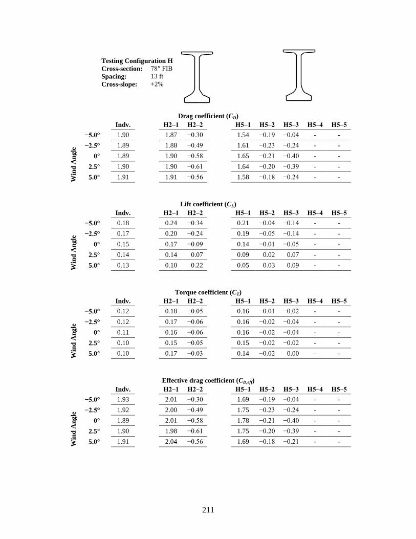
211
Testing Configuration H
Cross-section: 78″ FIB
Spacing: 13 ft
Cross-slope: +2%
Drag coefficient (CD)
Indv.
H2‒1 H2‒2
H5‒1 H5‒2 H5‒3 H5‒4 H5‒5
Win
d A
ng
le
−5.0°
1.90
1.87 −0.30
1.54 −0.19 −0.04 - -
−2.5°
1.89
1.88 −0.49
1.61 −0.23 −0.24 - -
+0.0°
1.89
1.90 −0.58
1.65 −0.21 −0.40 - -
+2.5°
1.90
1.90 −0.61
1.64 −0.20 −0.39 - -
+5.0°
1.91
1.91 −0.56
1.58 −0.18 −0.24 - -
M0‒0 M0‒0 M0‒0 M0‒0 M0‒0 M0‒0 M0‒0 M0‒0 M0‒0 M0‒0
Lift coefficient (CL)
Indv.
H2‒1 H2‒2
H5‒1 H5‒2 H5‒3 H5‒4 H5‒5
Win
d A
ng
le
−5.0°
0.18
0.24 −0.34
0.21 −0.04 −0.14 - -
−2.5°
0.17
0.20 −0.24
0.19 −0.05 −0.14 - -
+0.0°
0.15
0.17 −0.09
0.14 −0.01 −0.05 - -
+2.5°
0.14
0.14 +0.07
0.09 +0.02 +0.07 - -
+5.0°
0.13
0.10 +0.22
0.05 +0.03 +0.09 - -
M0‒0 M0‒0 M0‒0 M0‒0 M0‒0 M0‒0 M0‒0 M0‒0 M0‒0 M0‒0
Torque coefficient (CT)
Indv.
H2‒1 H2‒2
H5‒1 H5‒2 H5‒3 H5‒4 H5‒5
Win
d A
ng
le
−5.0°
0.12
0.18 −0.05
0.16 −0.01 −0.02 - -
−2.5°
0.12
0.17 −0.06
0.16 −0.02 −0.04 - -
+0.0°
0.11
0.16 −0.06
0.16 −0.02 −0.04 - -
+2.5°
0.10
0.15 −0.05
0.15 −0.02 −0.02 - -
+5.0°
0.10
0.17 −0.03
0.14 −0.02 +0.00 - -
M0‒0 M0‒0 M0‒0 M0‒0 M0‒0 M0‒0 M0‒0 M0‒0 M0‒0 M0‒0
Effective drag coefficient (CD,eff)
Indv.
H2‒1 H2‒2
H5‒1 H5‒2 H5‒3 H5‒4 H5‒5
Win
d A
ng
le
−5.0°
1.93
2.01 −0.30
1.69 −0.19 −0.04 - -
−2.5°
1.92
2.00 −0.49
1.75 −0.23 −0.24 - -
+0.0°
1.89
2.01 −0.58
1.78 −0.21 −0.40 - -
+2.5°
1.90
1.98 −0.61
1.75 −0.20 −0.39 - -
+5.0°
1.91
2.04 −0.56
1.69 −0.18 −0.21 - -
M0‒0 M0‒0 M0‒0 M0‒0 M0‒0 M0‒0 M0‒0 M0‒0 M0‒0 M0‒0
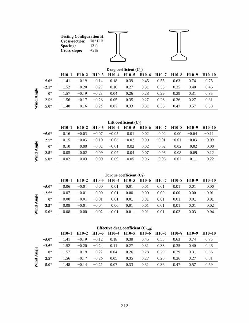
212
Testing Configuration H
Cross-section: 78″ FIB
Spacing: 13 ft
Cross-slope: +2%
Drag coefficient (CD)
H10‒1 H10‒2 H10‒3 H10‒4 H10‒5 H10‒6 H10‒7 H10‒8 H10‒9 H10‒10
Win
d A
ng
le
−5.0°
1.41 −0.19 −0.14 0.18 0.39 0.45 0.55 0.63 0.74 0.75
−2.5°
1.52 −0.20 −0.27 0.10 0.27 0.31 0.33 0.35 0.40 0.46
+0.0°
1.57 −0.19 −0.23 0.04 0.26 0.28 0.29 0.29 0.31 0.35
+2.5°
1.56 −0.17 −0.26 0.05 0.35 0.27 0.26 0.26 0.27 0.31
+5.0°
1.48 −0.16 −0.25 0.07 0.33 0.31 0.36 0.47 0.57 0.58
M0‒0 M0‒0 M0‒0 M0‒0 M0‒0 M0‒0 M0‒0 M0‒0 M0‒0 M0‒0
Lift coefficient (CL)
H10‒1 H10‒2 H10‒3 H10‒4 H10‒5 H10‒6 H10‒7 H10‒8 H10‒9 H10‒10
Win
d A
ng
le
−5.0°
0.16 −0.03 −0.07 −0.05 +0.01 0.02 +0.02 +0.00 −0.04 −0.11
−2.5°
0.15 −0.03 −0.10 −0.06 −0.02 0.00 −0.01 −0.01 −0.03 −0.09
+0.0°
0.10 +0.00 −0.02 −0.01 +0.02 0.02 +0.02 +0.02 +0.02 +0.00
+2.5°
0.05 +0.02 +0.09 +0.07 +0.04 0.07 +0.08 +0.08 +0.09 +0.12
+5.0°
0.02 +0.03 +0.09 +0.09 +0.05 0.06 +0.06 +0.07 +0.11 +0.22
M0‒0 M0‒0 M0‒0 M0‒0 M0‒0 M0‒0 M0‒0 M0‒0 M0‒0 M0‒0
Torque coefficient (CT)
H10‒1 H10‒2 H10‒3 H10‒4 H10‒5 H10‒6 H10‒7 H10‒8 H10‒9 H10‒10
Win
d A
ng
le
−5.0°
0.06 −0.01 +0.00 +0.01 0.01 0.01 0.01 0.01 0.01 +0.00
−2.5°
0.07 −0.01 +0.00 +0.01 0.00 0.00 0.00 0.00 0.00 −0.01
+0.0°
0.08 −0.01 −0.01 +0.01 0.01 0.01 0.01 0.01 0.01 +0.01
+2.5°
0.08 −0.01 −0.04 +0.00 0.01 0.01 0.01 0.01 0.01 +0.02
+5.0°
0.08 +0.00 −0.02 −0.01 0.01 0.01 0.01 0.02 0.03 +0.04
M0‒0 M0‒0 M0‒0 M0‒0 M0‒0 M0‒0 M0‒0 M0‒0 M0‒0 M0‒0
Effective drag coefficient (CD,eff)
H10‒1 H10‒2 H10‒3 H10‒4 H10‒5 H10‒6 H10‒7 H10‒8 H10‒9 H10‒10
Win
d A
ng
le
−5.0°
1.41 −0.19 −0.12 0.18 0.39 0.45 0.55 0.63 0.74 0.75
−2.5°
1.52 −0.20 −0.24 0.11 0.27 0.31 0.33 0.35 0.40 0.46
+0.0°
1.57 −0.19 −0.22 0.04 0.26 0.28 0.29 0.29 0.31 0.35
+2.5°
1.56 −0.17 −0.26 0.05 0.35 0.27 0.26 0.26 0.27 0.31
+5.0°
1.48 −0.14 −0.25 0.07 0.33 0.31 0.36 0.47 0.57 0.59
M0‒0 M0‒0 M0‒0 M0‒0 M0‒0 M0‒0 M0‒0 M0‒0 M0‒0 M0‒0
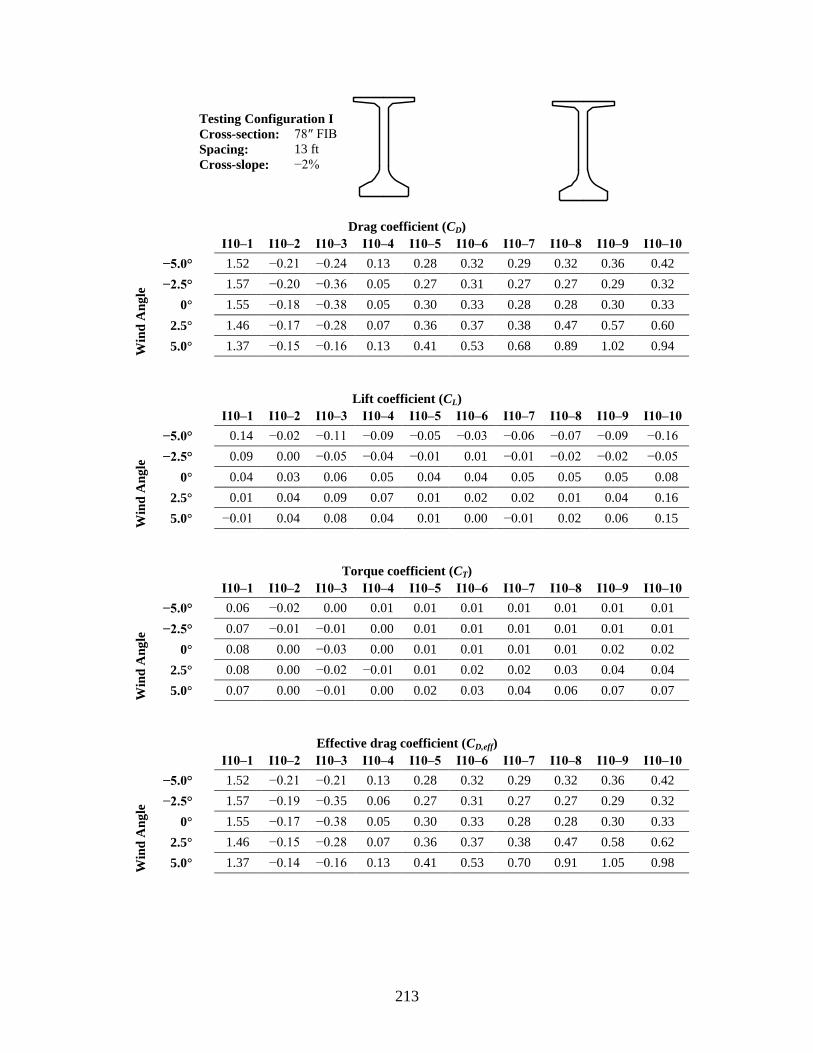
213
Testing Configuration I
Cross-section: 78″ FIB
Spacing: 13 ft
Cross-slope: −2%
Drag coefficient (CD)
I10‒1 I10‒2 I10‒3 I10‒4 I10‒5 I10‒6 I10‒7 I10‒8 I10‒9 I10‒10
Win
d A
ng
le
−5.0°
1.52 −0.21 −0.24 0.13 0.28 0.32 0.29 0.32 0.36 0.42
−2.5°
1.57 −0.20 −0.36 0.05 0.27 0.31 0.27 0.27 0.29 0.32
+0.0°
1.55 −0.18 −0.38 0.05 0.30 0.33 0.28 0.28 0.30 0.33
+2.5°
1.46 −0.17 −0.28 0.07 0.36 0.37 0.38 0.47 0.57 0.60
+5.0°
1.37 −0.15 −0.16 0.13 0.41 0.53 0.68 0.89 1.02 0.94
M0‒0 M0‒0 M0‒0 M0‒0 M0‒0 M0‒0 M0‒0 M0‒0 M0‒0 M0‒0
Lift coefficient (CL)
I10‒1 I10‒2 I10‒3 I10‒4 I10‒5 I10‒6 I10‒7 I10‒8 I10‒9 I10‒10
Win
d A
ng
le
−5.0°
+0.14 −0.02 −0.11 −0.09 −0.05 −0.03 −0.06 −0.07 −0.09 −0.16
−2.5°
+0.09 +0.00 −0.05 −0.04 −0.01 +0.01 −0.01 −0.02 −0.02 −0.05
+0.0°
+0.04 +0.03 +0.06 +0.05 +0.04 +0.04 +0.05 +0.05 +0.05 +0.08
+2.5°
+0.01 +0.04 +0.09 +0.07 +0.01 +0.02 +0.02 +0.01 +0.04 +0.16
+5.0°
−0.01 +0.04 +0.08 +0.04 +0.01 +0.00 −0.01 +0.02 +0.06 +0.15
M0‒0 M0‒0 M0‒0 M0‒0 M0‒0 M0‒0 M0‒0 M0‒0 M0‒0 M0‒0
Torque coefficient (CT)
I10‒1 I10‒2 I10‒3 I10‒4 I10‒5 I10‒6 I10‒7 I10‒8 I10‒9 I10‒10
Win
d A
ng
le
−5.0°
0.06 −0.02 +0.00 +0.01 0.01 0.01 0.01 0.01 0.01 0.01
−2.5°
0.07 −0.01 −0.01 +0.00 0.01 0.01 0.01 0.01 0.01 0.01
+0.0°
0.08 +0.00 −0.03 +0.00 0.01 0.01 0.01 0.01 0.02 0.02
+2.5°
0.08 +0.00 −0.02 −0.01 0.01 0.02 0.02 0.03 0.04 0.04
+5.0°
0.07 +0.00 −0.01 +0.00 0.02 0.03 0.04 0.06 0.07 0.07
M0‒0 M0‒0 M0‒0 M0‒0 M0‒0 M0‒0 M0‒0 M0‒0 M0‒0 M0‒0
Effective drag coefficient (CD,eff)
I10‒1 I10‒2 I10‒3 I10‒4 I10‒5 I10‒6 I10‒7 I10‒8 I10‒9 I10‒10
Win
d A
ng
le
−5.0°
1.52 −0.21 −0.21 0.13 0.28 0.32 0.29 0.32 0.36 0.42
−2.5°
1.57 −0.19 −0.35 0.06 0.27 0.31 0.27 0.27 0.29 0.32
+0.0°
1.55 −0.17 −0.38 0.05 0.30 0.33 0.28 0.28 0.30 0.33
+2.5°
1.46 −0.15 −0.28 0.07 0.36 0.37 0.38 0.47 0.58 0.62
+5.0°
1.37 −0.14 −0.16 0.13 0.41 0.53 0.70 0.91 1.05 0.98
M0‒0 M0‒0 M0‒0 M0‒0 M0‒0 M0‒0 M0‒0 M0‒0 M0‒0 M0‒0
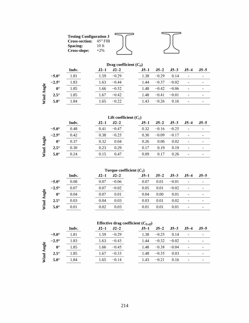
214
Testing Configuration J
Cross-section: 45″ FIB
Spacing: 10 ft
Cross-slope: +2%
Drag coefficient (CD)
Indv.
J2‒1 J2‒2
J5‒1 J5‒2 J5‒3 J5‒4 J5‒5
Win
d A
ng
le
−5.0°
1.81
1.59 −0.29
1.38 −0.29 +0.14 - -
−2.5°
1.83
1.63 −0.44
1.44 −0.37 −0.02 - -
+0.0°
1.85
1.66 −0.52
1.48 −0.42 −0.06 - -
+2.5°
1.85
1.67 −0.42
1.48 −0.41 −0.01 - -
+5.0°
1.84
1.65 −0.22
1.43 −0.26 +0.16 - -
M0‒0 M0‒0 M0‒0 M0‒0 M0‒0 M0‒0 M0‒0 M0‒0 M0‒0 M0‒0
Lift coefficient (CL)
Indv.
J2‒1 J2‒2
J5‒1 J5‒2 J5‒3 J5‒4 J5‒5
Win
d A
ng
le
−5.0°
0.48
0.41 −0.47
0.32 −0.16 −0.25 - -
−2.5°
0.42
0.38 −0.25
0.30 −0.09 −0.17 - -
+0.0°
0.37
0.32 +0.04
0.26 +0.06 +0.02 - -
+2.5°
0.30
0.23 +0.29
0.17 +0.19 +0.19 - -
+5.0°
0.24
0.15 +0.47
0.09 +0.17 +0.26 - -
M0‒0 M0‒0 M0‒0 M0‒0 M0‒0 M0‒0 M0‒0 M0‒0 M0‒0 M0‒0
Torque coefficient (CT)
Indv.
J2‒1 J2‒2
J5‒1 J5‒2 J5‒3 J5‒4 J5‒5
Win
d A
ng
le
−5.0°
0.08
0.07 −0.06
0.07 0.01 −0.01 - -
−2.5°
0.07
0.07 −0.02
0.05 0.01 −0.02 - -
+0.0°
0.04
0.07 +0.01
0.04 0.00 +0.01 - -
+2.5°
0.03
0.04 +0.03
0.03 0.01 +0.02 - -
+5.0°
0.01
0.02 +0.03
0.01 0.01 +0.01 - -
M0‒0 M0‒0 M0‒0 M0‒0 M0‒0 M0‒0 M0‒0 M0‒0 M0‒0 M0‒0
Effective drag coefficient (CD,eff)
Indv.
J2‒1 J2‒2
J5‒1 J5‒2 J5‒3 J5‒4 J5‒5
Win
d A
ng
le
−5.0°
1.81
1.59 −0.29
1.38 −0.25 +0.14 - -
−2.5°
1.83
1.63 −0.43
1.44 −0.32 −0.02 - -
+0.0°
1.85
1.66 −0.45
1.48 −0.38 −0.04 - -
+2.5°
1.85
1.67 −0.33
1.48 −0.35 +0.03 - -
+5.0°
1.84
1.65 −0.14
1.43 −0.21 +0.16 - -
M0‒0 M0‒0 M0‒0 M0‒0 M0‒0 M0‒0 M0‒0 M0‒0 M0‒0 M0‒0
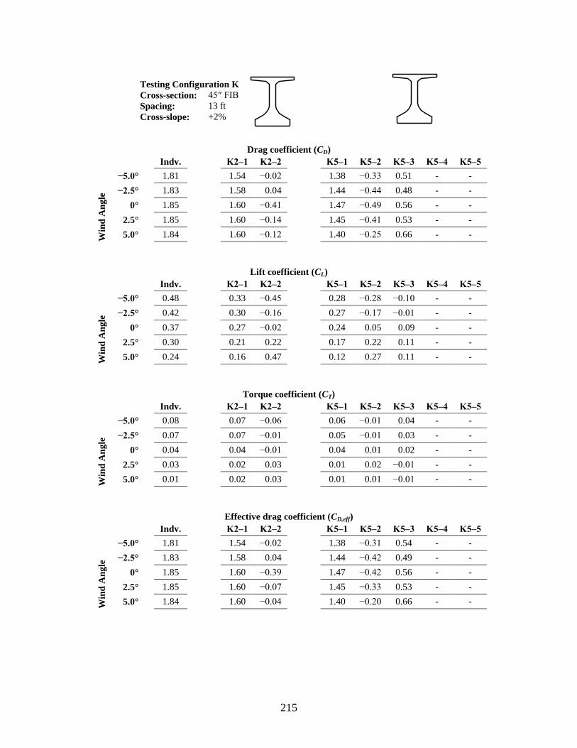
215
Testing Configuration K
Cross-section: 45″ FIB
Spacing: 13 ft
Cross-slope: +2%
Drag coefficient (CD)
Indv.
K2‒1 K2‒2
K5‒1 K5‒2 K5‒3 K5‒4 K5‒5
Win
d A
ng
le
−5.0°
1.81
1.54 −0.02
1.38 −0.33 0.51 - -
−2.5°
1.83
1.58 +0.04
1.44 −0.44 0.48 - -
+0.0°
1.85
1.60 −0.41
1.47 −0.49 0.56 - -
+2.5°
1.85
1.60 −0.14
1.45 −0.41 0.53 - -
+5.0°
1.84
1.60 −0.12
1.40 −0.25 0.66 - -
M0‒0 M0‒0 M0‒0 M0‒0 M0‒0 M0‒0 M0‒0 M0‒0 M0‒0 M0‒0
Lift coefficient (CL)
Indv.
K2‒1 K2‒2
K5‒1 K5‒2 K5‒3 K5‒4 K5‒5
Win
d A
ng
le
−5.0°
0.48
0.33 −0.45
0.28 −0.28 −0.10 - -
−2.5°
0.42
0.30 −0.16
0.27 −0.17 −0.01 - -
+0.0°
0.37
0.27 −0.02
0.24 +0.05 +0.09 - -
+2.5°
0.30
0.21 +0.22
0.17 +0.22 +0.11 - -
+5.0°
0.24
0.16 +0.47
0.12 +0.27 +0.11 - -
M0‒0 M0‒0 M0‒0 M0‒0 M0‒0 M0‒0 M0‒0 M0‒0 M0‒0 M0‒0
Torque coefficient (CT)
Indv.
K2‒1 K2‒2
K5‒1 K5‒2 K5‒3 K5‒4 K5‒5
Win
d A
ng
le
−5.0°
0.08
0.07 −0.06
0.06 −0.01 +0.04 - -
−2.5°
0.07
0.07 −0.01
0.05 −0.01 +0.03 - -
+0.0°
0.04
0.04 −0.01
0.04 +0.01 +0.02 - -
+2.5°
0.03
0.02 +0.03
0.01 +0.02 −0.01 - -
+5.0°
0.01
0.02 +0.03
0.01 +0.01 −0.01 - -
M0‒0 M0‒0 M0‒0 M0‒0 M0‒0 M0‒0 M0‒0 M0‒0 M0‒0 M0‒0
Effective drag coefficient (CD,eff)
Indv.
K2‒1 K2‒2
K5‒1 K5‒2 K5‒3 K5‒4 K5‒5
Win
d A
ng
le
−5.0°
1.81
1.54 −0.02
1.38 −0.31 0.54 - -
−2.5°
1.83
1.58 +0.04
1.44 −0.42 0.49 - -
+0.0°
1.85
1.60 −0.39
1.47 −0.42 0.56 - -
+2.5°
1.85
1.60 −0.07
1.45 −0.33 0.53 - -
+5.0°
1.84
1.60 −0.04
1.40 −0.20 0.66 - -
M0‒0 M0‒0 M0‒0 M0‒0 M0‒0 M0‒0 M0‒0 M0‒0 M0‒0 M0‒0
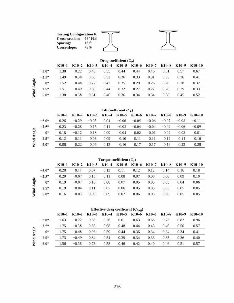
216
Testing Configuration K
Cross-section: 45″ FIB
Spacing: 13 ft
Cross-slope: +2%
Drag coefficient (CD)
K10‒1 K10‒2 K10‒3 K10‒4 K10‒5 K10‒6 K10‒7 K10‒8 K10‒9 K10‒10
Win
d A
ng
le
−5.0°
1.38 −0.22 0.48 0.55 0.44 0.44 0.46 0.51 0.57 0.67
−2.5°
1.49 −0.38 0.63 0.52 0.36 0.33 0.31 0.33 0.36 0.41
+0.0°
1.52 −0.48 0.72 0.47 0.35 0.29 0.26 0.26 0.28 0.32
+2.5°
1.51 −0.49 0.69 0.44 0.32 0.27 0.27 0.28 0.29 0.33
+5.0°
1.38 −0.38 0.61 0.46 0.36 0.34 0.34 0.38 0.45 0.52
M0‒0 M0‒0 M0‒0 M0‒0 M0‒0 M0‒0 M0‒0 M0‒0 M0‒0 M0‒0
Lift coefficient (CL)
K10‒1 K10‒2 K10‒3 K10‒4 K10‒5 K10‒6 K10‒7 K10‒8 K10‒9 K10‒10
Win
d A
ng
le
−5.0°
0.26 −0.29 −0.03 0.04 −0.06 −0.05 −0.06 −0.07 −0.08 −0.11
−2.5°
0.23 −0.28 +0.15 0.11 −0.03 −0.04 −0.04 −0.04 −0.06 −0.09
+0.0°
0.18 −0.12 +0.18 0.09 +0.04 +0.02 +0.01 +0.02 +0.02 +0.01
+2.5°
0.12 +0.11 +0.08 0.09 +0.10 +0.11 +0.11 +0.12 +0.14 +0.16
+5.0°
0.08 +0.22 +0.06 0.13 +0.16 +0.17 +0.17 +0.18 +0.22 +0.28
M0‒0 M0‒0 M0‒0 M0‒0 M0‒0 M0‒0 M0‒0 M0‒0 M0‒0 M0‒0
Torque coefficient (CT)
K10‒1 K10‒2 K10‒3 K10‒4 K10‒5 K10‒6 K10‒7 K10‒8 K10‒9 K10‒10
Win
d A
ng
le
−5.0°
0.20 −0.11 0.07 0.13 0.11 0.12 0.12 0.14 0.16 0.18
−2.5°
0.20 −0.07 0.15 0.11 0.08 0.07 0.08 0.08 0.09 0.10
+0.0°
0.19 −0.07 0.16 0.08 0.07 0.05 0.05 0.05 0.04 0.06
+2.5°
0.19 −0.04 0.11 0.07 0.06 0.05 0.05 0.05 0.05 0.05
+5.0°
0.16 −0.03 0.09 0.09 0.07 0.06 0.05 0.06 0.05 0.05
M0‒0 M0‒0 M0‒0 M0‒0 M0‒0 M0‒0 M0‒0 M0‒0 M0‒0 M0‒0
Effective drag coefficient (CD,eff)
K10‒1 K10‒2 K10‒3 K10‒4 K10‒5 K10‒6 K10‒7 K10‒8 K10‒9 K10‒10
Win
d A
ng
le
−5.0°
1.63 −0.22 0.58 0.76 0.61 0.63 0.65 0.75 0.82 0.96
−2.5°
1.75 −0.38 0.86 0.68 0.48 0.44 0.43 0.46 0.50 0.57
+0.0°
1.75 −0.48 0.96 0.59 0.44 0.36 0.34 0.34 0.34 0.41
+2.5°
1.73 −0.49 0.84 0.54 0.39 0.34 0.33 0.35 0.36 0.40
+5.0°
1.56 −0.38 0.73 0.58 0.46 0.42 0.40 0.46 0.51 0.57
M0‒0 M0‒0 M0‒0 M0‒0 M0‒0 M0‒0 M0‒0 M0‒0 M0‒0 M0‒0
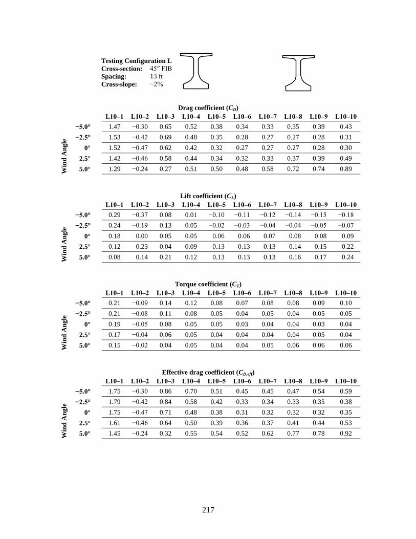
217
Testing Configuration L
Cross-section: 45″ FIB
Spacing: 13 ft
Cross-slope: −2%
Drag coefficient (CD)
L10‒1 L10‒2 L10‒3 L10‒4 L10‒5 L10‒6 L10‒7 L10‒8 L10‒9 L10‒10
Win
d A
ng
le
−5.0°
1.47 −0.30 0.65 0.52 0.38 0.34 0.33 0.35 0.39 0.43
−2.5°
1.53 −0.42 0.69 0.48 0.35 0.28 0.27 0.27 0.28 0.31
+0.0°
1.52 −0.47 0.62 0.42 0.32 0.27 0.27 0.27 0.28 0.30
+2.5°
1.42 −0.46 0.58 0.44 0.34 0.32 0.33 0.37 0.39 0.49
+5.0°
1.29 −0.24 0.27 0.51 0.50 0.48 0.58 0.72 0.74 0.89
M0‒0 M0‒0 M0‒0 M0‒0 M0‒0 M0‒0 M0‒0 M0‒0 M0‒0 M0‒0
Lift coefficient (CL)
L10‒1 L10‒2 L10‒3 L10‒4 L10‒5 L10‒6 L10‒7 L10‒8 L10‒9 L10‒10
Win
d A
ng
le
−5.0°
0.29 −0.37 0.08 0.01 −0.10 −0.11 −0.12 −0.14 −0.15 −0.18
−2.5°
0.24 −0.19 0.13 0.05 −0.02 −0.03 −0.04 −0.04 −0.05 −0.07
+0.0°
0.18 +0.00 0.05 0.05 +0.06 +0.06 +0.07 +0.08 +0.08 +0.09
+2.5°
0.12 +0.23 0.04 0.09 +0.13 +0.13 +0.13 +0.14 +0.15 +0.22
+5.0°
0.08 +0.14 0.21 0.12 +0.13 +0.13 +0.13 +0.16 +0.17 +0.24
M0‒0 M0‒0 M0‒0 M0‒0 M0‒0 M0‒0 M0‒0 M0‒0 M0‒0 M0‒0
Torque coefficient (CT)
L10‒1 L10‒2 L10‒3 L10‒4 L10‒5 L10‒6 L10‒7 L10‒8 L10‒9 L10‒10
Win
d A
ng
le
−5.0°
0.21 −0.09 0.14 0.12 0.08 0.07 0.08 0.08 0.09 0.10
−2.5°
0.21 −0.08 0.11 0.08 0.05 0.04 0.05 0.04 0.05 0.05
+0.0°
0.19 −0.05 0.08 0.05 0.05 0.03 0.04 0.04 0.03 0.04
+2.5°
0.17 −0.04 0.06 0.05 0.04 0.04 0.04 0.04 0.05 0.04
+5.0°
0.15 −0.02 0.04 0.05 0.04 0.04 0.05 0.06 0.06 0.06
M0‒0 M0‒0 M0‒0 M0‒0 M0‒0 M0‒0 M0‒0 M0‒0 M0‒0 M0‒0
Effective drag coefficient (CD,eff)
L10‒1 L10‒2 L10‒3 L10‒4 L10‒5 L10‒6 L10‒7 L10‒8 L10‒9 L10‒10
Win
d A
ng
le
−5.0°
1.75 −0.30 0.86 0.70 0.51 0.45 0.45 0.47 0.54 0.59
−2.5°
1.79 −0.42 0.84 0.58 0.42 0.33 0.34 0.33 0.35 0.38
+0.0°
1.75 −0.47 0.71 0.48 0.38 0.31 0.32 0.32 0.32 0.35
+2.5°
1.61 −0.46 0.64 0.50 0.39 0.36 0.37 0.41 0.44 0.53
+5.0°
1.45 −0.24 0.32 0.55 0.54 0.52 0.62 0.77 0.78 0.92
M0‒0 M0‒0 M0‒0 M0‒0 M0‒0 M0‒0 M0‒0 M0‒0 M0‒0 M0‒0
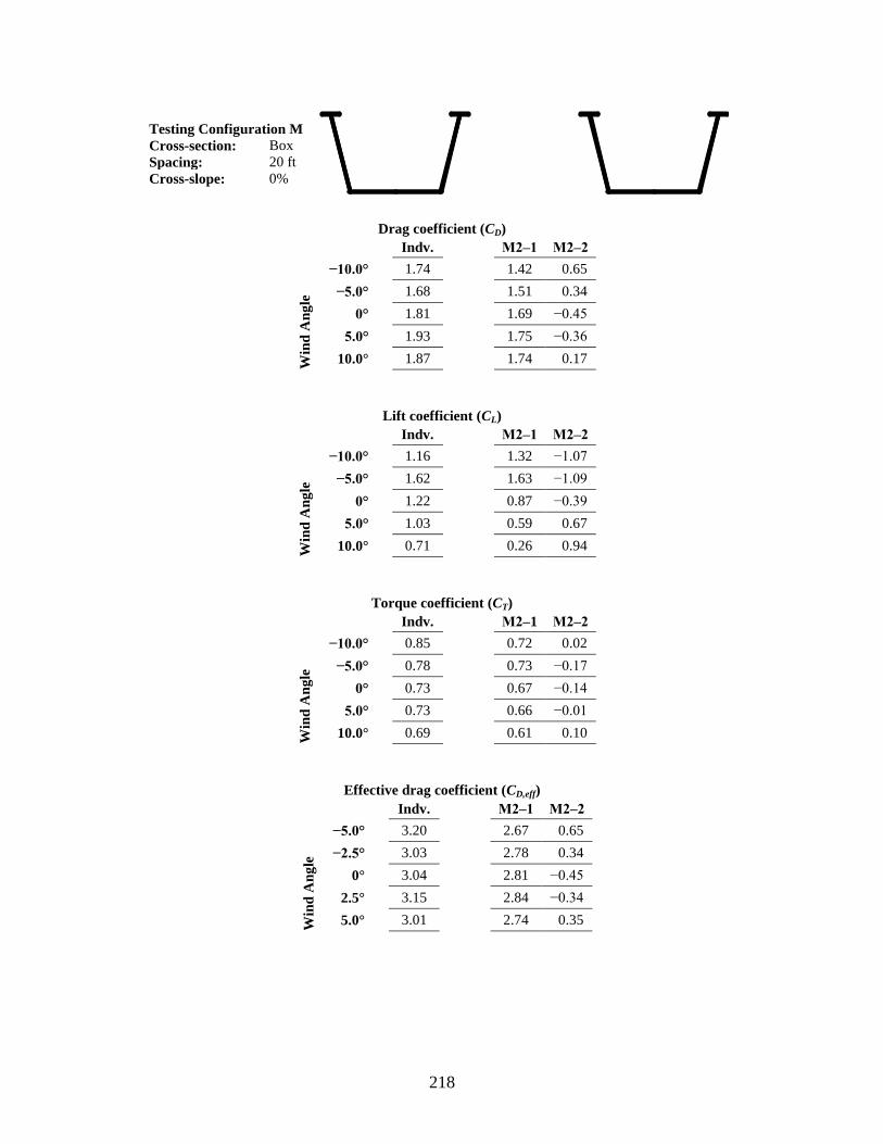
218
Testing Configuration M
Cross-section: Box
Spacing: 20 ft
Cross-slope: 0%
Drag coefficient (CD)
Indv.
M2‒1 M2‒2
Win
d A
ng
le
−10.0°
1.74
1.42 +0.65
−5.0°
1.68
1.51 +0.34
0°
1.81
1.69 −0.45
5.0°
1.93
1.75 −0.36
10.0°
1.87
1.74 +0.17
M0‒0 M0‒0 M0‒0 M0‒0
Lift coefficient (CL)
Indv.
M2‒1 M2‒2
Win
d A
ng
le
−10.0°
1.16
1.32 −1.07
−5.0°
1.62
1.63 −1.09
0°
1.22
0.87 −0.39
5.0°
1.03
0.59 +0.67
10.0°
0.71
0.26 +0.94
M0‒0 M0‒0 M0‒0 M0‒0
Torque coefficient (CT)
Indv.
M2‒1 M2‒2
Win
d A
ng
le
−10.0°
0.85
0.72 +0.02
−5.0°
0.78
0.73 −0.17
0°
0.73
0.67 −0.14
5.0°
0.73
0.66 −0.01
10.0°
0.69
0.61 +0.10
M0‒0 M0‒0 M0‒0 M0‒0
Effective drag coefficient (CD,eff)
Indv.
M2‒1 M2‒2
Win
d A
ng
le
−5.0°
3.20
2.67 +0.65
−2.5°
3.03
2.78 +0.34
+0.0°
3.04
2.81 −0.45
+2.5°
3.15
2.84 −0.34
+5.0°
3.01
2.74 +0.35
M0‒0 M0‒0 M0‒0 M0‒0
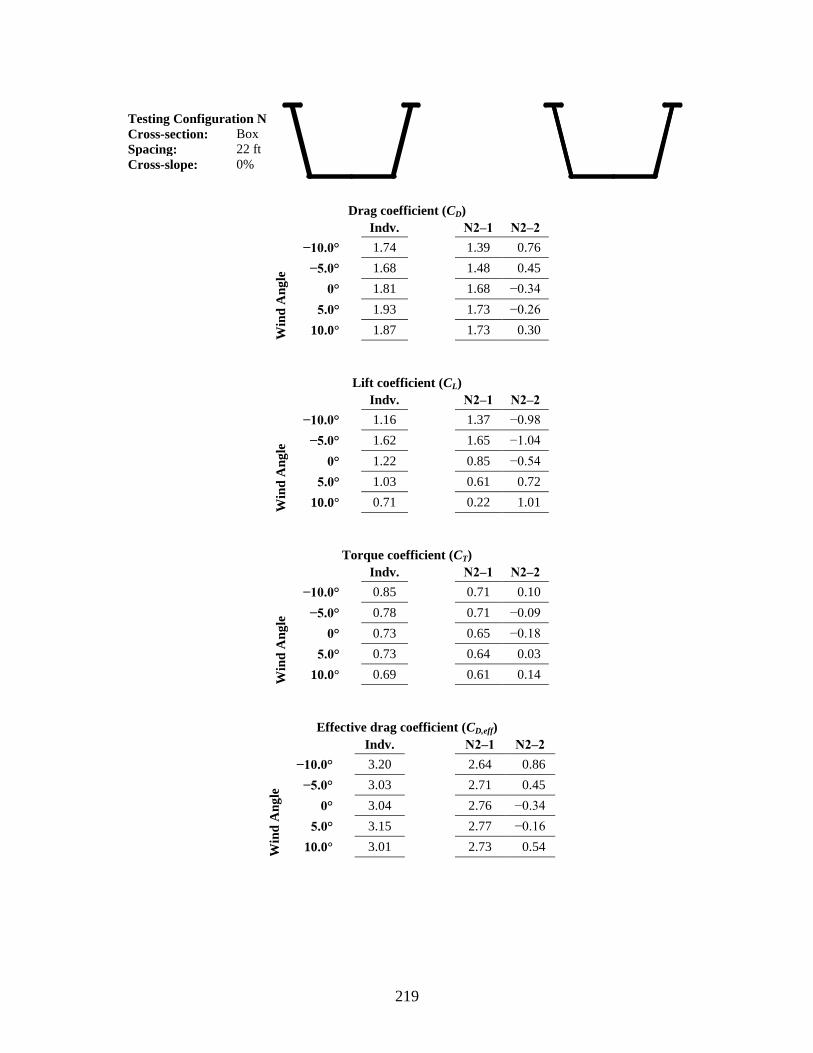
219
Testing Configuration N
Cross-section: Box
Spacing: 22 ft
Cross-slope: 0%
Drag coefficient (CD)
Indv.
N2‒1 N2‒2
Win
d A
ng
le
−10.0°
1.74
1.39 +0.76
−5.0°
1.68
1.48 +0.45
0°
1.81
1.68 −0.34
5.0°
1.93
1.73 −0.26
10.0°
1.87
1.73 +0.30
M0‒0 M0‒0 M0‒0 M0‒0
Lift coefficient (CL)
Indv.
N2‒1 N2‒2
Win
d A
ng
le
−10.0°
1.16
1.37 −0.98
−5.0°
1.62
1.65 −1.04
0°
1.22
0.85 −0.54
5.0°
1.03
0.61 +0.72
10.0°
0.71
0.22 +1.01
M0‒0 M0‒0 M0‒0 M0‒0
Torque coefficient (CT)
Indv.
N2‒1 N2‒2
Win
d A
ng
le
−10.0°
0.85
0.71 +0.10
−5.0°
0.78
0.71 −0.09
0°
0.73
0.65 −0.18
5.0°
0.73
0.64 +0.03
10.0°
0.69
0.61 +0.14
M0‒0 M0‒0 M0‒0 M0‒0
Effective drag coefficient (CD,eff)
Indv.
N2‒1 N2‒2
Win
d A
ng
le
−10.0°
3.20
2.64 +0.86
−5.0°
3.03
2.71 +0.45
0°
3.04
2.76 −0.34
5.0°
3.15
2.77 −0.16
10.0°
3.01
2.73 +0.54
M0‒0 M0‒0 M0‒0 M0‒0
220
APPENDIX C
CROSS-SECTIONAL PROPERTIES OF FLORIDA-I BEAMS
In this study, finite element models were analyzed to evaluate the lateral stability of
Florida-I Beams (FIBs). In each model, the FIBs were modeled using warping beams,
specialized beam elements available in the ADINA finite element code, which require the
calculation of a comprehensive set of cross-sectional properties. This appendix provides
mathematical definitions of all such properties and corresponding numeric values that were
calculated for each FIB cross-sectional shape.
Definitions of the cross-sectional properties that are required to use the warping beam
element in ADINA are listed in Table C-1. Each property requires the evaluation of an integral
over the area of the cross-section, in which the integrands are written in terms of coordinates x
and y, referenced to the geometric centroid of the section (Figure C-1). Some properties also
require knowledge of the warping function, ψ(x,y), which represents the torsionally-induced out-
of-plane warping displacements per rate of twist at every point on the cross-section. (The units of
ψ are therefore in/(rad/in) or in2.)
For general cross-sectional shapes (e.g., an FIB), analytical (closed-form) solutions for
ψ(x,y) do not exist; instead the warping field ψ(x,y) must be solved numerically. In this study, the
calculation of ψ(x,y) for each FIB shape was accomplished by discretizing the cross-sectional
shape into a high-resolution mesh of thousands of two-dimensional triangular elements, and then
employing a finite element approach to solve the governing differential equation.
In general, solutions for ψ(x,y) change depending on the assumed location of the center of
twist. In the literature, the term ‘warping function’ typically refers to a particular solution (ψ in
Table C-1) corresponding to a state of pure torsion, i.e., torsion about the shear center. As a
result, prior knowledge of the location of the shear center is required to compute several of the
221
warping beam properties. However, it is possible to calculate the coordinates of the shear center,
xs and ys (Table C-1), using an alternative solution to the warping function (ψc), where the center
of twist is assumed to be located at the centroid of the section. Therefore, two different warping
functions were computed for each FIB section: first the section centroid was used to compute ψc
and then the location of the shear center, obtained from ψc, was used to compute ψ as well as the
remaining cross-sectional properties.
Because all FIB cross-sections are symmetric about the y-axis, Ixy, xs, Ixr, and Iωr have a
value of zero (0) by definition. The remaining cross-sectional properties calculated for each FIB
shape are summarized in Table C-2.
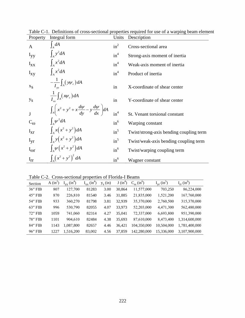
222
Table C-1. Definitions of cross-sectional properties required for use of a warping beam element
Property Integral form Units Description
A AdA
in2 Cross-sectional area
Iyy 2
Ay dA
in4 Strong-axis moment of inertia
Ixx 2
Ax dA
in4 Weak-axis moment of inertia
Ixy 2
Ax dA
in4 Product of inertia
xs
1c
Ayy
y dAI
in
X-coordinate of shear center
ys
1c
Axx
x dAI
in
Y-coordinate of shear center
J
2 2
A
d dx y x y dA
dy dx
in4 St. Venant torsional constant
Cω 2
AdA
in6 Warping constant
Ixr 2 2
Ax x y dA
in5 Twist/strong-axis bending coupling term
Iyr 2 2
Ay x y dA
in5 Twist/weak-axis bending coupling term
Iωr 2 2
Ax y dA
in6 Twist/warping coupling term
Irr 2
2 2
Ax y dA
in6 Wagner constant
Table C-2. Cross-sectional properties of Florida-I Beams
Section ωA (in2) Iyy (in
4) Ixx (in
4) ys (in) ωJ (in
4) Cω (in
6) Iyr (in
5) Irr (in
6)
36″ FIB 807 127,700 81283 3.00 30,864 11,577,000 703,250 86,224,000
45″ FIB 870 226,810 81540 3.46 31,885 21,835,000 1,521,200 167,760,000
54″ FIB 933 360,270 81798 3.81 32,939 35,370,000 2,760,500 315,370,000
63″ FIB 996 530,790 82055 4.07 33,973 52,203,000 4,471,300 562,480,000
72″ FIB 1059 741,060 82314 4.27 35,041 72,337,000 6,693,800 951,390,000
78″ FIB 1101 904,610 82484 4.38 35,693 87,610,000 8,473,400 1,314,600,000
84″ FIB 1143 1,087,800 82657 4.46 36,421 104,350,000 10,504,000 1,781,400,000
96″ FIB 1227 1,516,200 83,002 4.56 37,859 142,280,000 15,336,000 3,107,900,000
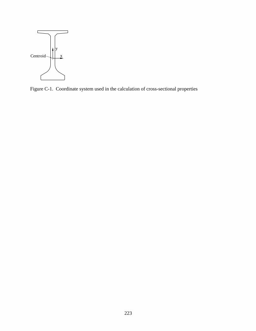
223
Centroid x
y
Figure C-1. Coordinate system used in the calculation of cross-sectional properties

224
APPENDIX D
PROPERTIES OF FLORIDA BEARING PADS
This appendix includes computed stiffnesses (Table D-1) for several standard types of
FDOT bearing pad, produced using the calculation methods discussed in Chapter 6. Pad types D,
E, F, G, H, J, and K are current designs intended for use with Florida-I Beams (FIBs), while pad
types A, B, and C were formerly provided for use with Florida Bulb-Tees (FBTs). While Florida
Bulb-Tee girders are no longer used in new bridge designs, they are still in service in existing
bridges throughout Florida, thus stiffness data for pad types A, B, and C are included here for
completeness. Each pad type is defined by four design parameters (Figure D-1): the plan-view
length and width (L and W), elastomer shear modulus (G), and the number of internal elastomer
layers (n).
Linear stiffnesses corresponding to bearing pad shear, torsion, axial compression,
overturning roll (about the y-axis) for the zero-slope condition, and bending roll (about the x-
axis) are presented in Table D-1. Unlike bending roll, overturning roll stiffness varies depending
on the total axial load (i.e., girder weight) when the slope angle is non-zero. Consequently,
nonlinear overturning roll stiffness curves for several combinations slope angle and axial load
are provided on the following pages.
On the pages that follow, each curve corresponds to a unique combination of pad type,
slope angle, and axial load (the quantities noted in kips). On each curve, Kr is the initial
overturning roll stiffness in kip-ft/rad.
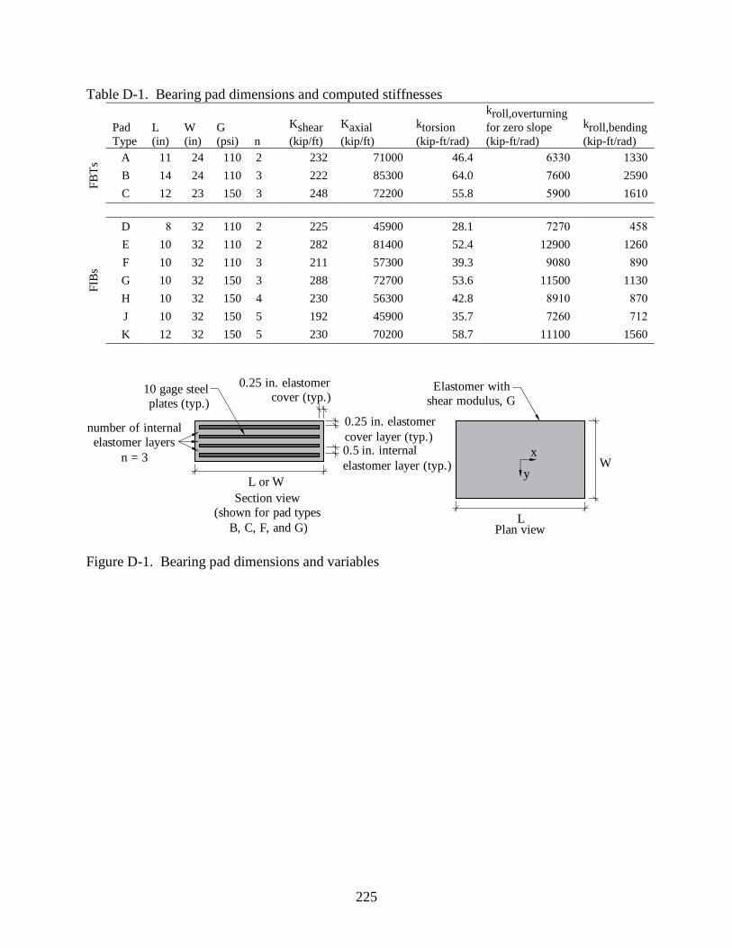
225
Table D-1. Bearing pad dimensions and computed stiffnesses
Pad
Type
L
(in)
W
(in)
G
(psi) n
Kshear
(kip/ft)
Kaxial
(kip/ft)
ktorsion
(kip-ft/rad)
kroll,overturning
for zero slope
(kip-ft/rad)
kroll,bending
(kip-ft/rad)
FB
Ts
A 11 24 110 2 232 71000 46.4 6330 1330
B 14 24 110 3 222 85300 64.0 7600 2590
C 12 23 150 3 248 72200 55.8 5900 1610
FIB
s
D 8 32 110 2 225 45900 28.1 7270 458
E 10 32 110 2 282 81400 52.4 12900 1260
F 10 32 110 3 211 57300 39.3 9080 890
G 10 32 150 3 288 72700 53.6 11500 1130
H 10 32 150 4 230 56300 42.8 8910 870
J 10 32 150 5 192 45900 35.7 7260 712
K 12 32 150 5 230 70200 58.7 11100 1560
W
LPlan view
10 gage steel
plates (typ.)
0.5 in. internal
elastomer layer (typ.)
L or W
0.25 in. elastomer
cover (typ.)
0.25 in. elastomer
cover layer (typ.)
Section view
(shown for pad types
B, C, F, and G)
number of internal
elastomer layers
n = 3
Elastomer with
shear modulus, G
x
y
Figure D-1. Bearing pad dimensions and variables
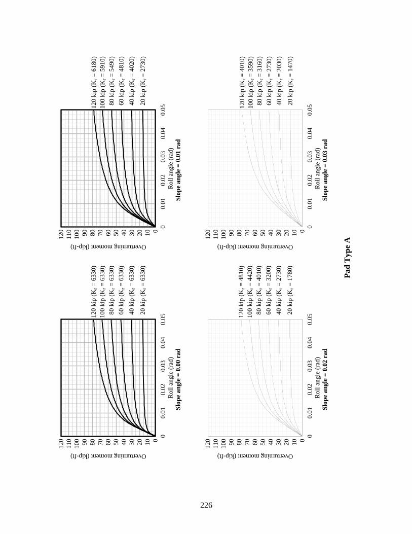
226
Pad
Typ
e A
Roll
an
gle
(ra
d)
Slo
pe
an
gle
= 0
.01 r
ad
Overturning moment (kip-ft)
00.0
10
.02
0.0
30
.04
0.0
5
0
10
20
30
40
50
60
70
80
90
10
0
11
0
12
0
02
0 k
ip (
Kr =
27
30)
04
0 k
ip (
Kr =
40
20)
06
0 k
ip (
Kr =
48
10)
08
0 k
ip (
Kr =
54
90)
10
0 k
ip (
Kr =
59
10)
12
0 k
ip (
Kr =
61
80)
Roll
an
gle
(ra
d)
Slo
pe
an
gle
= 0
.03 r
ad
Overturning moment (kip-ft)
00.0
10
.02
0.0
30
.04
0.0
5
0
10
20
30
40
50
60
70
80
90
10
0
11
0
12
0
02
0 k
ip (
Kr =
14
70)
04
0 k
ip (
Kr =
20
30)
06
0 k
ip (
Kr =
27
30)
08
0 k
ip (
Kr =
31
60)
10
0 k
ip (
Kr =
35
90)
12
0 k
ip (
Kr =
40
10)
Ro
ll a
ng
le (
rad
)
Slo
pe
an
gle
= 0
.00 r
ad
Overturning moment (kip-ft)
00.0
10
.02
0.0
30
.04
0.0
5
0
10
20
30
40
50
60
70
80
90
100
110
120
020
kip
(K
r =
63
30)
040
kip
(K
r =
63
30)
060
kip
(K
r =
63
30)
080
kip
(K
r =
63
30)
100
kip
(K
r =
63
30)
120
kip
(K
r =
63
30)
Ro
ll a
ng
le (
rad
)
Slo
pe
an
gle
= 0
.02 r
ad
Overturning moment (kip-ft)
00.0
10
.02
0.0
30
.04
0.0
5
0
10
20
30
40
50
60
70
80
90
100
110
120
020
kip
(K
r =
17
80)
040
kip
(K
r =
27
30)
060
kip
(K
r =
32
00)
080
kip
(K
r =
40
10)
100
kip
(K
r =
44
20)
120
kip
(K
r =
48
10)
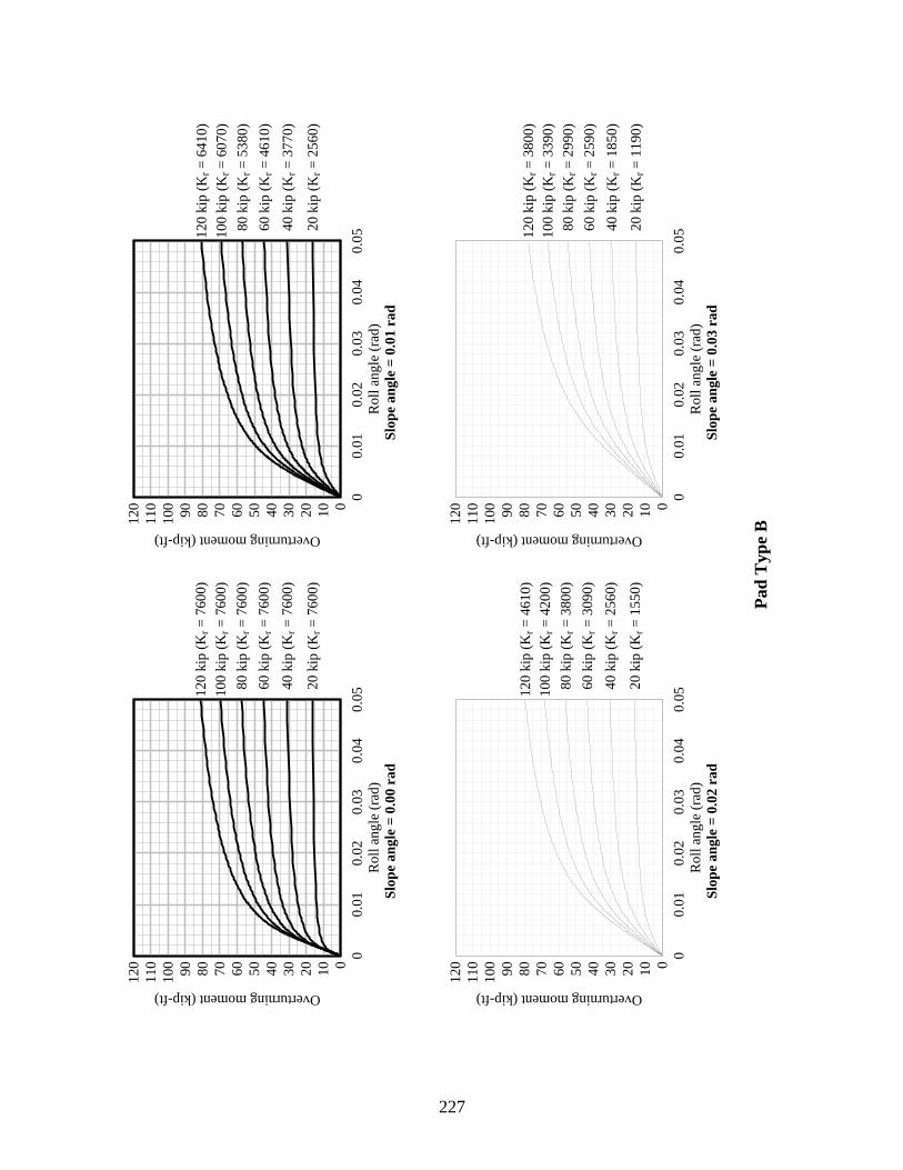
227
Pad
Typ
e B
Roll
an
gle
(ra
d)
Slo
pe
an
gle
= 0
.01 r
ad
Overturning moment (kip-ft)
00.0
10
.02
0.0
30
.04
0.0
5
0
10
20
30
40
50
60
70
80
90
10
0
11
0
12
0
02
0 k
ip (
Kr =
25
60)
04
0 k
ip (
Kr =
37
70)
06
0 k
ip (
Kr =
46
10)
08
0 k
ip (
Kr =
53
80)
10
0 k
ip (
Kr =
60
70)
12
0 k
ip (
Kr =
64
10)
Roll
an
gle
(ra
d)
Slo
pe
an
gle
= 0
.03 r
ad
Overturning moment (kip-ft)
00.0
10
.02
0.0
30
.04
0.0
5
0
10
20
30
40
50
60
70
80
90
10
0
11
0
12
0
02
0 k
ip (
Kr =
11
90)
04
0 k
ip (
Kr =
18
50)
06
0 k
ip (
Kr =
25
90)
08
0 k
ip (
Kr =
29
90)
10
0 k
ip (
Kr =
33
90)
12
0 k
ip (
Kr =
38
00)
Ro
ll a
ng
le (
rad
)
Slo
pe
an
gle
= 0
.00 r
ad
Overturning moment (kip-ft)
00.0
10
.02
0.0
30
.04
0.0
5
0
10
20
30
40
50
60
70
80
90
100
110
120
020
kip
(K
r =
76
00)
040
kip
(K
r =
76
00)
060
kip
(K
r =
76
00)
080
kip
(K
r =
76
00)
100
kip
(K
r =
76
00)
120
kip
(K
r =
76
00)
Ro
ll a
ng
le (
rad
)
Slo
pe
an
gle
= 0
.02 r
ad
Overturning moment (kip-ft)
00.0
10
.02
0.0
30
.04
0.0
5
0
10
20
30
40
50
60
70
80
90
100
110
120
020
kip
(K
r =
15
50)
040
kip
(K
r =
25
60)
060
kip
(K
r =
30
90)
080
kip
(K
r =
38
00)
100
kip
(K
r =
42
00)
120
kip
(K
r =
46
10)

228
Pad
Typ
e C
Roll
an
gle
(ra
d)
Slo
pe
an
gle
= 0
.01 r
ad
Overturning moment (kip-ft)
00.0
10
.02
0.0
30
.04
0.0
5
0
10
20
30
40
50
60
70
80
90
10
0
11
0
12
0
02
0 k
ip (
Kr =
22
70)
04
0 k
ip (
Kr =
33
60)
06
0 k
ip (
Kr =
43
60)
08
0 k
ip (
Kr =
49
40)
10
0 k
ip (
Kr =
52
40)
12
0 k
ip (
Kr =
56
50)
Roll
an
gle
(ra
d)
Slo
pe
an
gle
= 0
.03 r
ad
Overturning moment (kip-ft)
00.0
10
.02
0.0
30
.04
0.0
5
0
10
20
30
40
50
60
70
80
90
10
0
11
0
12
0
02
0 k
ip (
Kr =
12
10)
04
0 k
ip (
Kr =
18
70)
06
0 k
ip (
Kr =
22
20)
08
0 k
ip (
Kr =
26
80)
10
0 k
ip (
Kr =
30
40)
12
0 k
ip (
Kr =
33
30)
Ro
ll a
ng
le (
rad
)
Slo
pe
an
gle
= 0
.00 r
ad
Overturning moment (kip-ft)
00.0
10
.02
0.0
30
.04
0.0
5
0
10
20
30
40
50
60
70
80
90
100
110
120
020
kip
(K
r =
59
00)
040
kip
(K
r =
59
00)
060
kip
(K
r =
59
00)
080
kip
(K
r =
59
00)
100
kip
(K
r =
59
00)
120
kip
(K
r =
59
00)
Ro
ll a
ng
le (
rad
)
Slo
pe
an
gle
= 0
.02 r
ad
Overturning moment (kip-ft)
00.0
10
.02
0.0
30
.04
0.0
5
0
10
20
30
40
50
60
70
80
90
100
110
120
020
kip
(K
r =
15
30)
040
kip
(K
r =
22
20)
060
kip
(K
r =
29
50)
080
kip
(K
r =
33
20)
100
kip
(K
r =
40
10)
120
kip
(K
r =
43
70)
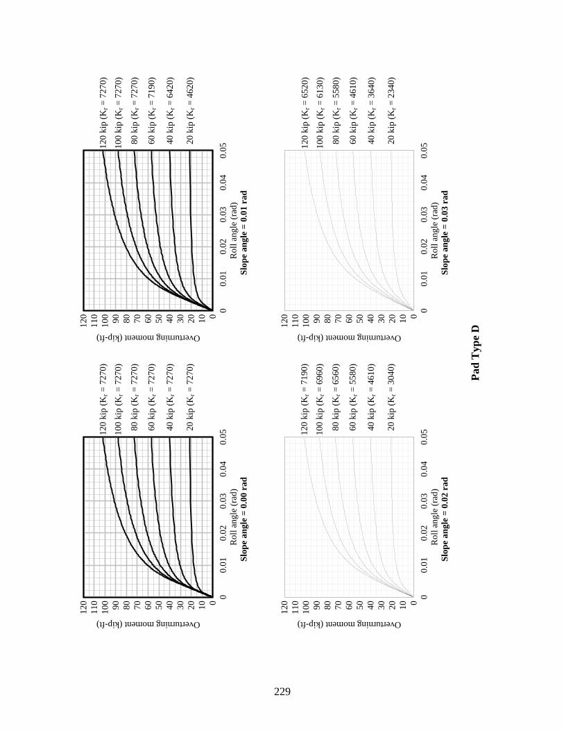
229
Pad
Typ
e D
Roll
an
gle
(ra
d)
Slo
pe
an
gle
= 0
.01 r
ad
Overturning moment (kip-ft)
00.0
10
.02
0.0
30
.04
0.0
5
0
10
20
30
40
50
60
70
80
90
10
0
11
0
12
0
02
0 k
ip (
Kr =
46
20)
04
0 k
ip (
Kr =
64
20)
06
0 k
ip (
Kr =
71
90)
08
0 k
ip (
Kr =
72
70)
10
0 k
ip (
Kr =
72
70)
12
0 k
ip (
Kr =
72
70)
Roll
an
gle
(ra
d)
Slo
pe
an
gle
= 0
.03 r
ad
Overturning moment (kip-ft)
00.0
10
.02
0.0
30
.04
0.0
5
0
10
20
30
40
50
60
70
80
90
10
0
11
0
12
0
02
0 k
ip (
Kr =
23
40)
04
0 k
ip (
Kr =
36
40)
06
0 k
ip (
Kr =
46
10)
08
0 k
ip (
Kr =
55
80)
10
0 k
ip (
Kr =
61
30)
12
0 k
ip (
Kr =
65
20)
Ro
ll a
ng
le (
rad
)
Slo
pe
an
gle
= 0
.00 r
ad
Overturning moment (kip-ft)
00.0
10
.02
0.0
30
.04
0.0
5
0
10
20
30
40
50
60
70
80
90
100
110
120
020
kip
(K
r =
72
70)
040
kip
(K
r =
72
70)
060
kip
(K
r =
72
70)
080
kip
(K
r =
72
70)
100
kip
(K
r =
72
70)
120
kip
(K
r =
72
70)
Ro
ll a
ng
le (
rad
)
Slo
pe
an
gle
= 0
.02 r
ad
Overturning moment (kip-ft)
00.0
10
.02
0.0
30
.04
0.0
5
0
10
20
30
40
50
60
70
80
90
100
110
120
020
kip
(K
r =
30
40)
040
kip
(K
r =
46
10)
060
kip
(K
r =
55
80)
080
kip
(K
r =
65
60)
100
kip
(K
r =
69
60)
120
kip
(K
r =
71
90)
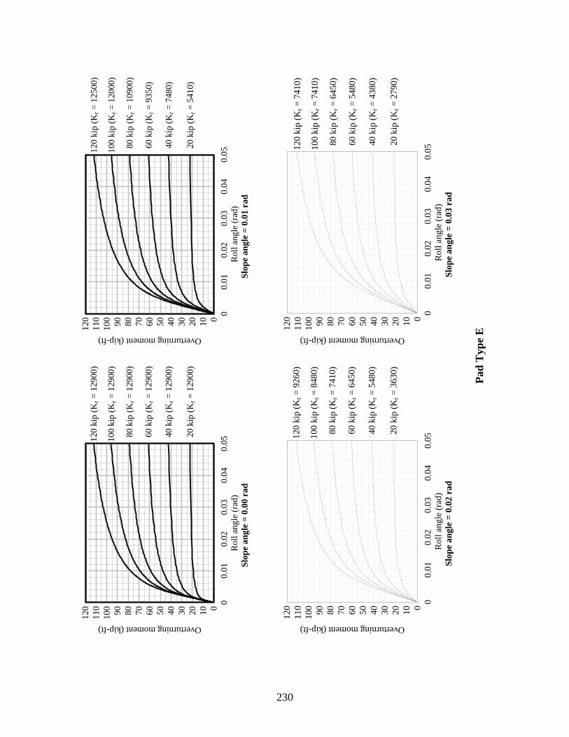
230
Pad
Typ
e E
Roll
angle
(ra
d)
Slo
pe
an
gle
= 0
.01 r
ad
Overturning moment (kip-ft)
00.0
10.0
20.0
30.0
40.0
5
0
10
20
30
40
50
60
70
80
90
100
110
120
020 k
ip (
Kr =
5410)
040 k
ip (
Kr =
7480)
060 k
ip (
Kr =
9350)
080 k
ip (
Kr =
10900)
100 k
ip (
Kr =
12000)
120 k
ip (
Kr =
12500)
Roll
an
gle
(ra
d)
Slo
pe
an
gle
= 0
.03 r
ad
Overturning moment (kip-ft)
00.0
10
.02
0.0
30
.04
0.0
5
0
10
20
30
40
50
60
70
80
90
10
0
11
0
12
0
02
0 k
ip (
Kr =
27
90)
04
0 k
ip (
Kr =
43
80)
06
0 k
ip (
Kr =
54
80)
08
0 k
ip (
Kr =
64
50)
10
0 k
ip (
Kr =
74
10)
12
0 k
ip (
Kr =
74
10)
Roll
angle
(ra
d)
Slo
pe
an
gle
= 0
.00 r
ad
Overturning moment (kip-ft)
00.0
10.0
20.0
30.0
40.0
5
0
10
20
30
40
50
60
70
80
90
100
110
120
020 k
ip (
Kr =
12900)
040 k
ip (
Kr =
12900)
060 k
ip (
Kr =
12900)
080 k
ip (
Kr =
12900)
100 k
ip (
Kr =
12900)
120 k
ip (
Kr =
12900)
Ro
ll a
ng
le (
rad
)
Slo
pe
an
gle
= 0
.02 r
ad
Overturning moment (kip-ft)
00.0
10
.02
0.0
30
.04
0.0
5
0
10
20
30
40
50
60
70
80
90
100
110
120
020
kip
(K
r =
36
30)
040
kip
(K
r =
54
80)
060
kip
(K
r =
64
50)
080
kip
(K
r =
74
10)
100
kip
(K
r =
84
80)
120
kip
(K
r =
92
60)
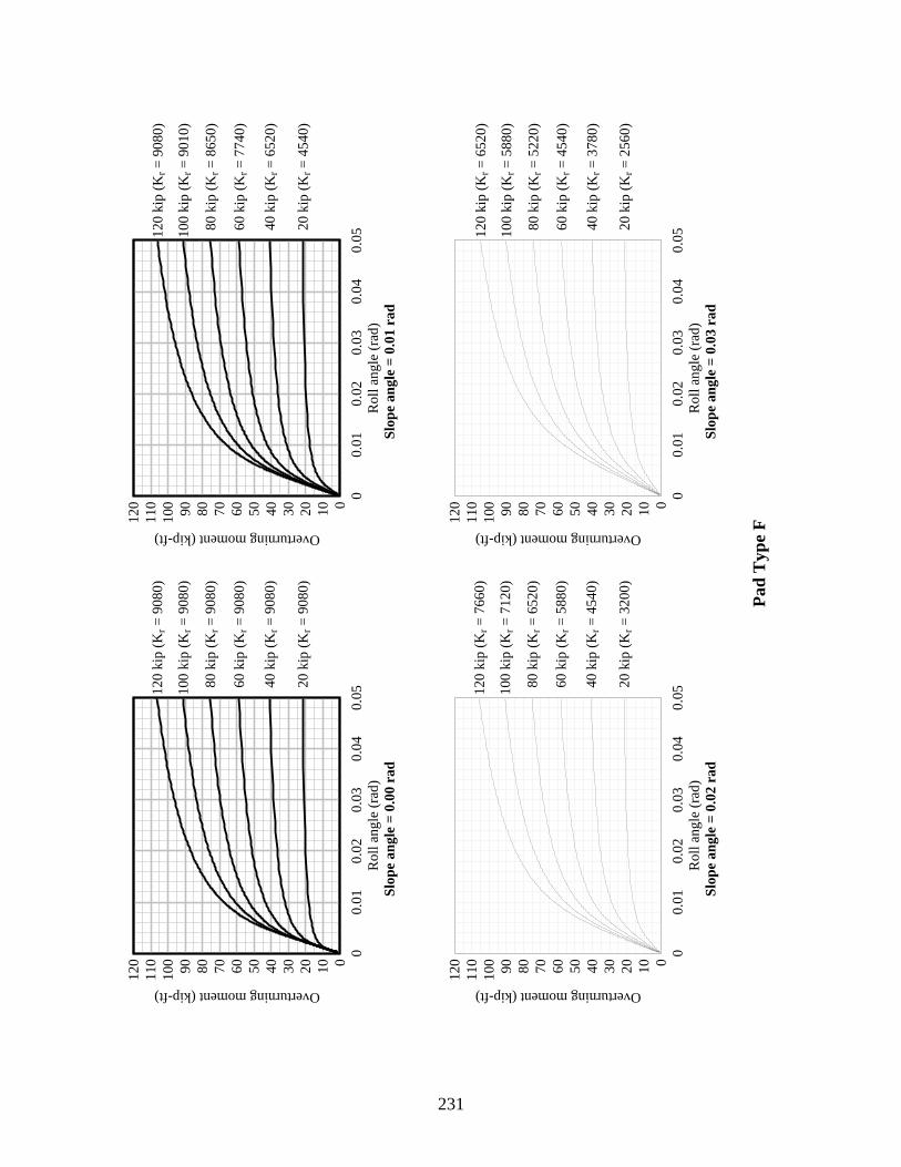
231
Pad
Typ
e F
Roll
an
gle
(ra
d)
Slo
pe
an
gle
= 0
.01 r
ad
Overturning moment (kip-ft)
00.0
10
.02
0.0
30
.04
0.0
5
0
10
20
30
40
50
60
70
80
90
10
0
11
0
12
0
02
0 k
ip (
Kr =
45
40)
04
0 k
ip (
Kr =
65
20)
06
0 k
ip (
Kr =
77
40)
08
0 k
ip (
Kr =
86
50)
10
0 k
ip (
Kr =
90
10)
12
0 k
ip (
Kr =
90
80)
Roll
an
gle
(ra
d)
Slo
pe
an
gle
= 0
.03 r
ad
Overturning moment (kip-ft)
00.0
10
.02
0.0
30
.04
0.0
5
0
10
20
30
40
50
60
70
80
90
10
0
11
0
12
0
02
0 k
ip (
Kr =
25
60)
04
0 k
ip (
Kr =
37
80)
06
0 k
ip (
Kr =
45
40)
08
0 k
ip (
Kr =
52
20)
10
0 k
ip (
Kr =
58
80)
12
0 k
ip (
Kr =
65
20)
Ro
ll a
ng
le (
rad
)
Slo
pe
an
gle
= 0
.00 r
ad
Overturning moment (kip-ft)
00.0
10
.02
0.0
30
.04
0.0
5
0
10
20
30
40
50
60
70
80
90
100
110
120
020
kip
(K
r =
90
80)
040
kip
(K
r =
90
80)
060
kip
(K
r =
90
80)
080
kip
(K
r =
90
80)
100
kip
(K
r =
90
80)
120
kip
(K
r =
90
80)
Ro
ll a
ng
le (
rad
)
Slo
pe
an
gle
= 0
.02 r
ad
Overturning moment (kip-ft)
00.0
10
.02
0.0
30
.04
0.0
5
0
10
20
30
40
50
60
70
80
90
100
110
120
020
kip
(K
r =
32
00)
040
kip
(K
r =
45
40)
060
kip
(K
r =
58
80)
080
kip
(K
r =
65
20)
100
kip
(K
r =
71
20)
120
kip
(K
r =
76
60)
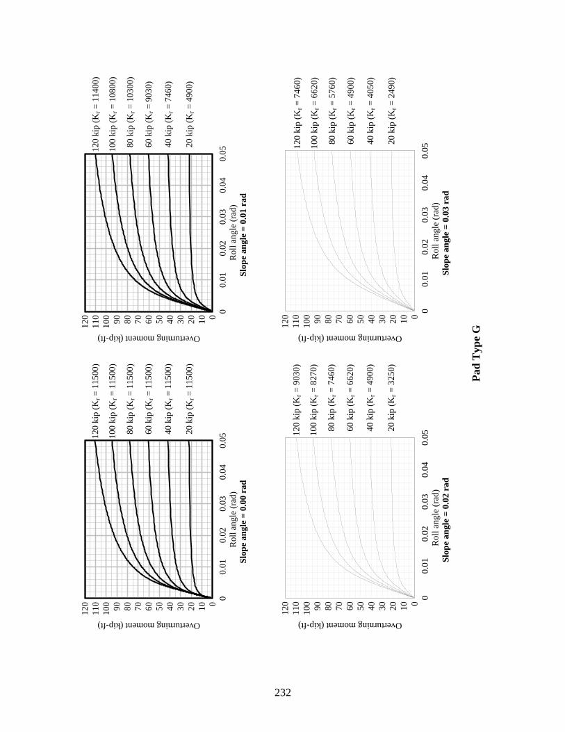
232
Pad
Typ
e G
Roll
angle
(ra
d)
Slo
pe
an
gle
= 0
.01 r
ad
Overturning moment (kip-ft)
00.0
10.0
20.0
30.0
40.0
5
0
10
20
30
40
50
60
70
80
90
100
110
120
020 k
ip (
Kr =
4900)
040 k
ip (
Kr =
7460)
060 k
ip (
Kr =
9030)
080 k
ip (
Kr =
10300)
100 k
ip (
Kr =
10800)
120 k
ip (
Kr =
11400)
Roll
an
gle
(ra
d)
Slo
pe
an
gle
= 0
.03 r
ad
Overturning moment (kip-ft)
00.0
10
.02
0.0
30
.04
0.0
5
0
10
20
30
40
50
60
70
80
90
10
0
11
0
12
0
02
0 k
ip (
Kr =
24
90)
04
0 k
ip (
Kr =
40
50)
06
0 k
ip (
Kr =
49
00)
08
0 k
ip (
Kr =
57
60)
10
0 k
ip (
Kr =
66
20)
12
0 k
ip (
Kr =
74
60)
Roll
angle
(ra
d)
Slo
pe
an
gle
= 0
.00 r
ad
Overturning moment (kip-ft)
00.0
10.0
20.0
30.0
40.0
5
0
10
20
30
40
50
60
70
80
90
100
110
120
020 k
ip (
Kr =
11500)
040 k
ip (
Kr =
11500)
060 k
ip (
Kr =
11500)
080 k
ip (
Kr =
11500)
100 k
ip (
Kr =
11500)
120 k
ip (
Kr =
11500)
Ro
ll a
ng
le (
rad
)
Slo
pe
an
gle
= 0
.02 r
ad
Overturning moment (kip-ft)
00.0
10
.02
0.0
30
.04
0.0
5
0
10
20
30
40
50
60
70
80
90
100
110
120
020
kip
(K
r =
32
50)
040
kip
(K
r =
49
00)
060
kip
(K
r =
66
20)
080
kip
(K
r =
74
60)
100
kip
(K
r =
82
70)
120
kip
(K
r =
90
30)

233
Pad
Typ
e H
Roll
an
gle
(ra
d)
Slo
pe
an
gle
= 0
.01 r
ad
Overturning moment (kip-ft)
00.0
10
.02
0.0
30
.04
0.0
5
0
10
20
30
40
50
60
70
80
90
10
0
11
0
12
0
02
0 k
ip (
Kr =
44
50)
04
0 k
ip (
Kr =
64
00)
06
0 k
ip (
Kr =
78
80)
08
0 k
ip (
Kr =
86
60)
10
0 k
ip (
Kr =
89
00)
12
0 k
ip (
Kr =
89
10)
Roll
an
gle
(ra
d)
Slo
pe
an
gle
= 0
.03 r
ad
Overturning moment (kip-ft)
00.0
10
.02
0.0
30
.04
0.0
5
0
10
20
30
40
50
60
70
80
90
10
0
11
0
12
0
02
0 k
ip (
Kr =
24
90)
04
0 k
ip (
Kr =
37
70)
06
0 k
ip (
Kr =
44
50)
08
0 k
ip (
Kr =
51
20)
10
0 k
ip (
Kr =
57
70)
12
0 k
ip (
Kr =
64
00)
Ro
ll a
ng
le (
rad
)
Slo
pe
an
gle
= 0
.00 r
ad
Overturning moment (kip-ft)
00.0
10
.02
0.0
30
.04
0.0
5
0
10
20
30
40
50
60
70
80
90
100
110
120
020
kip
(K
r =
89
10)
040
kip
(K
r =
89
10)
060
kip
(K
r =
89
10)
080
kip
(K
r =
89
10)
100
kip
(K
r =
89
10)
120
kip
(K
r =
89
10)
Ro
ll a
ng
le (
rad
)
Slo
pe
an
gle
= 0
.02 r
ad
Overturning moment (kip-ft)
00.0
10
.02
0.0
30
.04
0.0
5
0
10
20
30
40
50
60
70
80
90
100
110
120
020
kip
(K
r =
31
20)
040
kip
(K
r =
44
50)
060
kip
(K
r =
57
70)
080
kip
(K
r =
64
00)
100
kip
(K
r =
69
80)
120
kip
(K
r =
79
60)
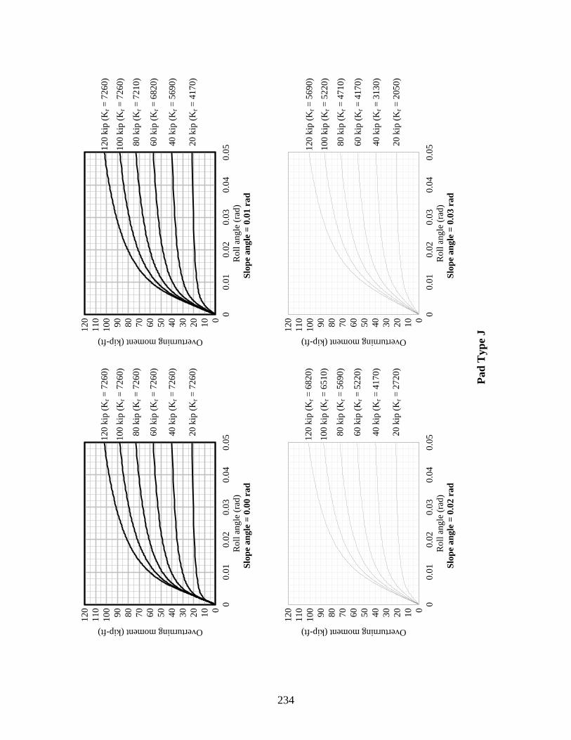
234
Pad
Typ
e J
Roll
an
gle
(ra
d)
Slo
pe
an
gle
= 0
.01 r
ad
Overturning moment (kip-ft)
00.0
10
.02
0.0
30
.04
0.0
5
0
10
20
30
40
50
60
70
80
90
10
0
11
0
12
0
02
0 k
ip (
Kr =
41
70)
04
0 k
ip (
Kr =
56
90)
06
0 k
ip (
Kr =
68
20)
08
0 k
ip (
Kr =
72
10)
10
0 k
ip (
Kr =
72
60)
12
0 k
ip (
Kr =
72
60)
Roll
an
gle
(ra
d)
Slo
pe
an
gle
= 0
.03 r
ad
Overturning moment (kip-ft)
00.0
10
.02
0.0
30
.04
0.0
5
0
10
20
30
40
50
60
70
80
90
10
0
11
0
12
0
02
0 k
ip (
Kr =
20
50)
04
0 k
ip (
Kr =
31
30)
06
0 k
ip (
Kr =
41
70)
08
0 k
ip (
Kr =
47
10)
10
0 k
ip (
Kr =
52
20)
12
0 k
ip (
Kr =
56
90)
Ro
ll a
ng
le (
rad
)
Slo
pe
an
gle
= 0
.00 r
ad
Overturning moment (kip-ft)
00.0
10
.02
0.0
30
.04
0.0
5
0
10
20
30
40
50
60
70
80
90
100
110
120
020
kip
(K
r =
72
60)
040
kip
(K
r =
72
60)
060
kip
(K
r =
72
60)
080
kip
(K
r =
72
60)
100
kip
(K
r =
72
60)
120
kip
(K
r =
72
60)
Ro
ll a
ng
le (
rad
)
Slo
pe
an
gle
= 0
.02 r
ad
Overturning moment (kip-ft)
00.0
10
.02
0.0
30
.04
0.0
5
0
10
20
30
40
50
60
70
80
90
100
110
120
020
kip
(K
r =
27
20)
040
kip
(K
r =
41
70)
060
kip
(K
r =
52
20)
080
kip
(K
r =
56
90)
100
kip
(K
r =
65
10)
120
kip
(K
r =
68
20)
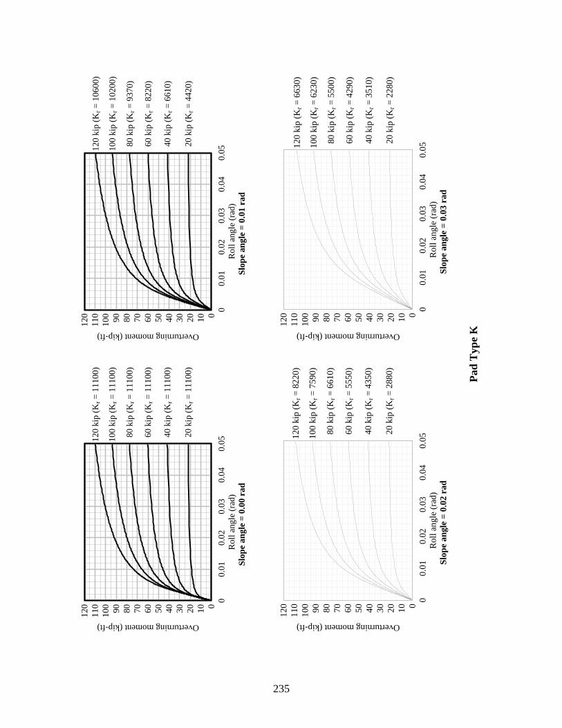
235
Pad
Typ
e K
Roll
angle
(ra
d)
Slo
pe
an
gle
= 0
.01 r
ad
Overturning moment (kip-ft)
00.0
10.0
20.0
30.0
40.0
5
0
10
20
30
40
50
60
70
80
90
100
110
120
020 k
ip (
Kr =
4420)
040 k
ip (
Kr =
6610)
060 k
ip (
Kr =
8220)
080 k
ip (
Kr =
9370)
100 k
ip (
Kr =
10200)
120 k
ip (
Kr =
10600)
Roll
an
gle
(ra
d)
Slo
pe
an
gle
= 0
.03 r
ad
Overturning moment (kip-ft)
00.0
10
.02
0.0
30
.04
0.0
5
0
10
20
30
40
50
60
70
80
90
10
0
11
0
12
0
02
0 k
ip (
Kr =
22
80)
04
0 k
ip (
Kr =
35
10)
06
0 k
ip (
Kr =
42
90)
08
0 k
ip (
Kr =
55
00)
10
0 k
ip (
Kr =
62
30)
12
0 k
ip (
Kr =
66
30)
Roll
angle
(ra
d)
Slo
pe
an
gle
= 0
.00 r
ad
Overturning moment (kip-ft)
00.0
10.0
20.0
30.0
40.0
5
0
10
20
30
40
50
60
70
80
90
100
110
120
020 k
ip (
Kr =
11100)
040 k
ip (
Kr =
11100)
060 k
ip (
Kr =
11100)
080 k
ip (
Kr =
11100)
100 k
ip (
Kr =
11100)
120 k
ip (
Kr =
11100)
Ro
ll a
ng
le (
rad
)
Slo
pe
an
gle
= 0
.02 r
ad
Overturning moment (kip-ft)
00.0
10
.02
0.0
30
.04
0.0
5
0
10
20
30
40
50
60
70
80
90
10
0
11
0
12
0
020
kip
(K
r =
28
80)
040
kip
(K
r =
43
50)
060
kip
(K
r =
55
50)
080
kip
(K
r =
66
10)
100
kip
(K
r =
75
90)
120
kip
(K
r =
82
20)
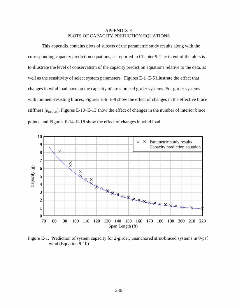
236
APPENDIX E
PLOTS OF CAPACITY PREDICTION EQUATIONS
This appendix contains plots of subsets of the parametric study results along with the
corresponding capacity prediction equations, as reported in Chapter 9. The intent of the plots is
to illustrate the level of conservatism of the capacity prediction equations relative to the data, as
well as the sensitivity of select system parameters. Figures E-1–E-5 illustrate the effect that
changes in wind load have on the capacity of strut-braced girder systems. For girder systems
with moment-resisting braces, Figures E-6–E-9 show the effect of changes in the effective brace
stiffness (kbrace), Figures E-10–E-13 show the effect of changes in the number of interior brace
points, and Figures E-14–E-18 show the effect of changes in wind load.
Figure E-1. Prediction of system capacity for 2-girder, unanchored strut-braced systems in 0-psf
wind (Equation 9-10)
Span Length (ft)
Cap
acit
y (
g)
70 80 90 100 110 120 130 140 150 160 170 180 190 200 210 220
0
1
2
3
4
5
6
7
8
9
10
70 80 90 100 110 120 130 140 150 160 170 180 190 200 210 220
0
1
2
3
4
5
6
7
8
9
10
Parametric study results
Capacity prediction equation
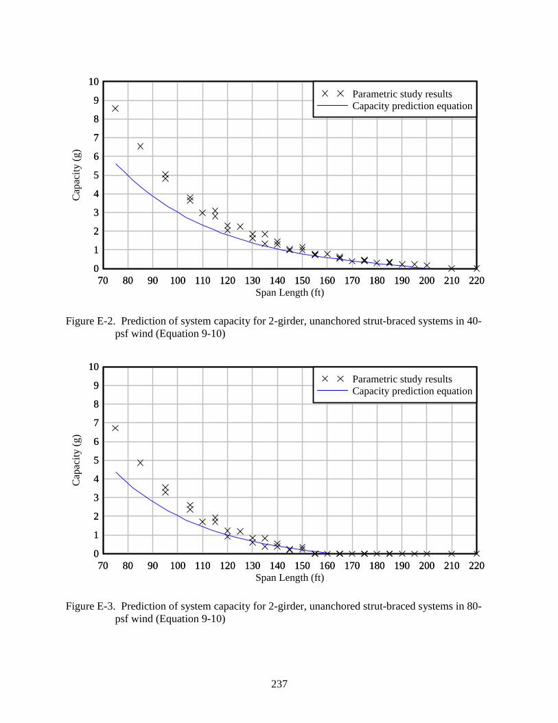
237
Figure E-2. Prediction of system capacity for 2-girder, unanchored strut-braced systems in 40-
psf wind (Equation 9-10)
Figure E-3. Prediction of system capacity for 2-girder, unanchored strut-braced systems in 80-
psf wind (Equation 9-10)
Span Length (ft)
Cap
acit
y (
g)
70 80 90 100 110 120 130 140 150 160 170 180 190 200 210 220
0
1
2
3
4
5
6
7
8
9
10
70 80 90 100 110 120 130 140 150 160 170 180 190 200 210 220
0
1
2
3
4
5
6
7
8
9
10
Parametric study results
Capacity prediction equation
Span Length (ft)
Cap
acit
y (
g)
70 80 90 100 110 120 130 140 150 160 170 180 190 200 210 220
0
1
2
3
4
5
6
7
8
9
10
70 80 90 100 110 120 130 140 150 160 170 180 190 200 210 220
0
1
2
3
4
5
6
7
8
9
10
Parametric study results
Capacity prediction equation
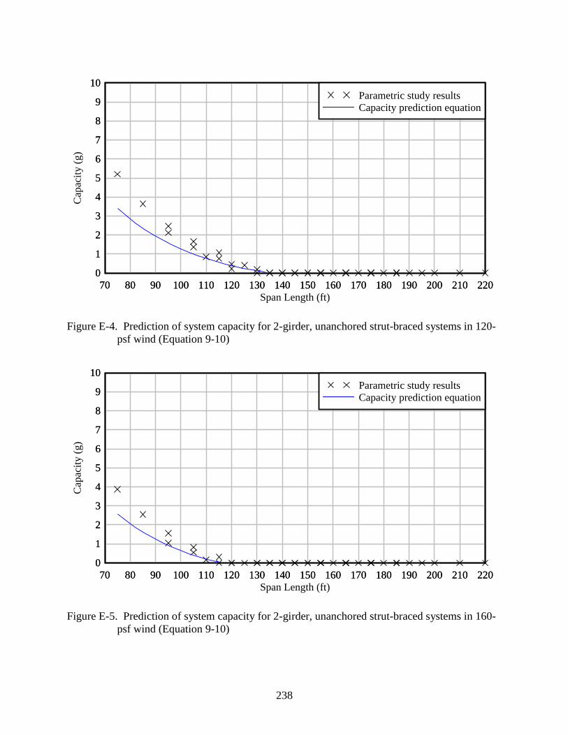
238
Figure E-4. Prediction of system capacity for 2-girder, unanchored strut-braced systems in 120-
psf wind (Equation 9-10)
Figure E-5. Prediction of system capacity for 2-girder, unanchored strut-braced systems in 160-
psf wind (Equation 9-10)
Span Length (ft)
Cap
acit
y (
g)
70 80 90 100 110 120 130 140 150 160 170 180 190 200 210 220
0
1
2
3
4
5
6
7
8
9
10
70 80 90 100 110 120 130 140 150 160 170 180 190 200 210 220
0
1
2
3
4
5
6
7
8
9
10
Parametric study results
Capacity prediction equation
Span Length (ft)
Cap
acit
y (
g)
70 80 90 100 110 120 130 140 150 160 170 180 190 200 210 220
0
1
2
3
4
5
6
7
8
9
10
70 80 90 100 110 120 130 140 150 160 170 180 190 200 210 220
0
1
2
3
4
5
6
7
8
9
10
Parametric study results
Capacity prediction equation
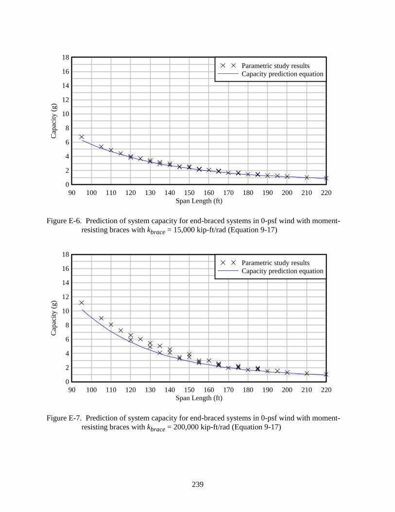
239
Figure E-6. Prediction of system capacity for end-braced systems in 0-psf wind with moment-
resisting braces with kbrace = 15,000 kip-ft/rad (Equation 9-17)
Figure E-7. Prediction of system capacity for end-braced systems in 0-psf wind with moment-
resisting braces with kbrace = 200,000 kip-ft/rad (Equation 9-17)
Span Length (ft)
Cap
acit
y (
g)
90 100 110 120 130 140 150 160 170 180 190 200 210 220
0
2
4
6
8
10
12
14
16
18
Parametric study results
Capacity prediction equation
Span Length (ft)
Cap
acit
y (
g)
90 100 110 120 130 140 150 160 170 180 190 200 210 220
0
2
4
6
8
10
12
14
16
18
Parametric study results
Capacity prediction equation
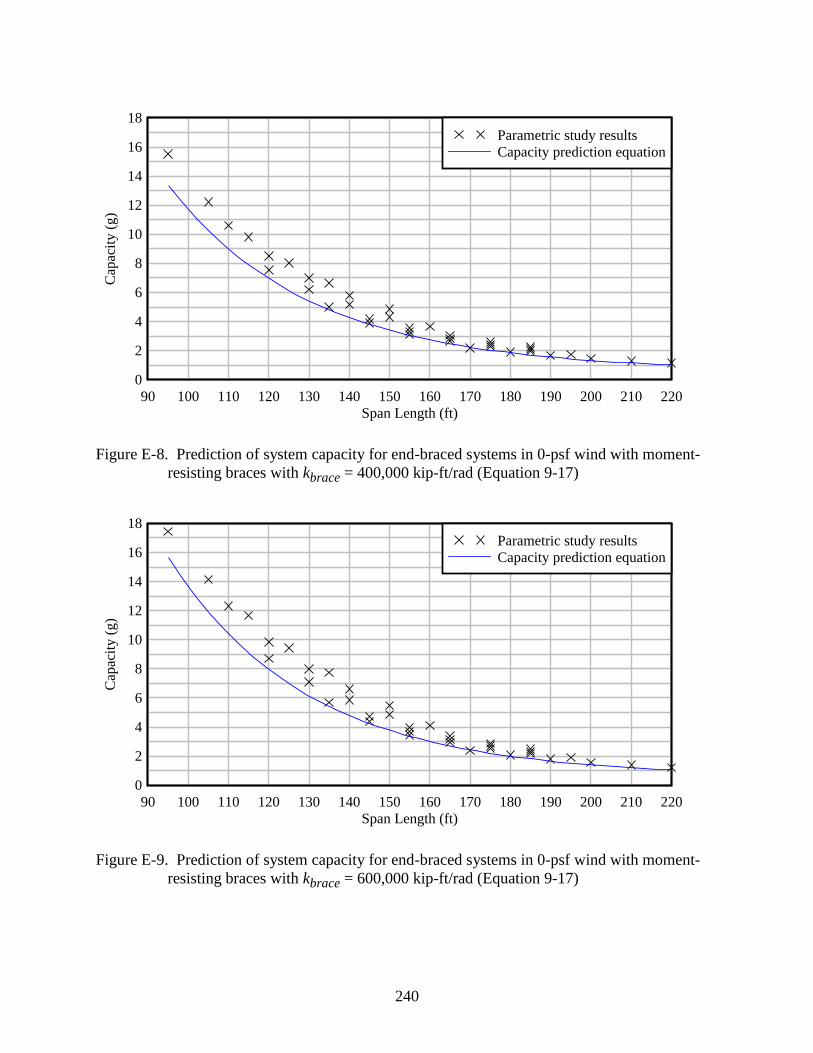
240
Figure E-8. Prediction of system capacity for end-braced systems in 0-psf wind with moment-
resisting braces with kbrace = 400,000 kip-ft/rad (Equation 9-17)
Figure E-9. Prediction of system capacity for end-braced systems in 0-psf wind with moment-
resisting braces with kbrace = 600,000 kip-ft/rad (Equation 9-17)
Span Length (ft)
Cap
acit
y (
g)
90 100 110 120 130 140 150 160 170 180 190 200 210 220
0
2
4
6
8
10
12
14
16
18
Parametric study results
Capacity prediction equation
Span Length (ft)
Cap
acit
y (
g)
90 100 110 120 130 140 150 160 170 180 190 200 210 220
0
2
4
6
8
10
12
14
16
18
Parametric study results
Capacity prediction equation
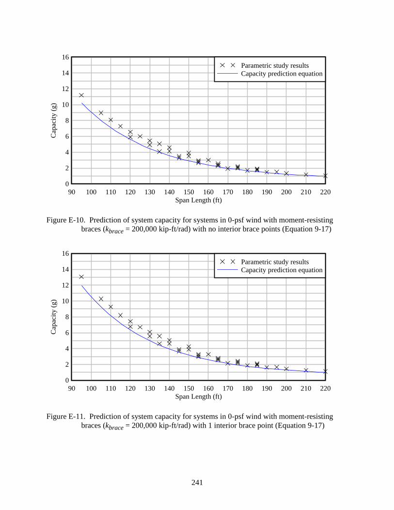
241
Figure E-10. Prediction of system capacity for systems in 0-psf wind with moment-resisting
braces (kbrace = 200,000 kip-ft/rad) with no interior brace points (Equation 9-17)
Figure E-11. Prediction of system capacity for systems in 0-psf wind with moment-resisting
braces (kbrace = 200,000 kip-ft/rad) with 1 interior brace point (Equation 9-17)
Span Length (ft)
Cap
acit
y (
g)
90 100 110 120 130 140 150 160 170 180 190 200 210 220
0
2
4
6
8
10
12
14
16
Parametric study results
Capacity prediction equation
Span Length (ft)
Cap
acit
y (
g)
90 100 110 120 130 140 150 160 170 180 190 200 210 220
0
2
4
6
8
10
12
14
16
Parametric study results
Capacity prediction equation
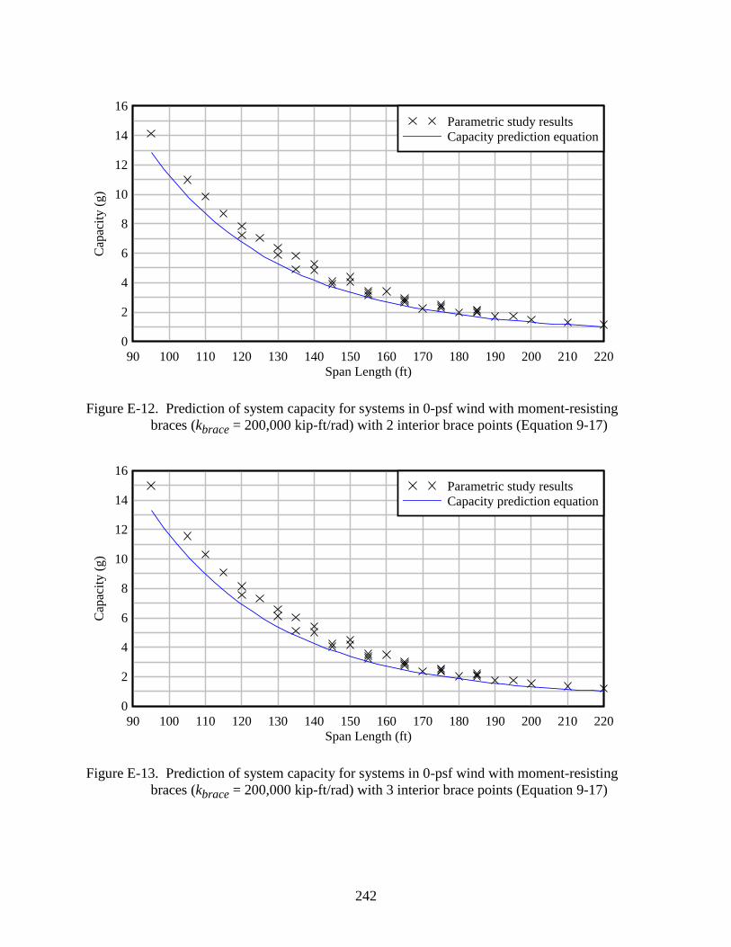
242
Figure E-12. Prediction of system capacity for systems in 0-psf wind with moment-resisting
braces (kbrace = 200,000 kip-ft/rad) with 2 interior brace points (Equation 9-17)
Figure E-13. Prediction of system capacity for systems in 0-psf wind with moment-resisting
braces (kbrace = 200,000 kip-ft/rad) with 3 interior brace points (Equation 9-17)
Span Length (ft)
Cap
acit
y (
g)
90 100 110 120 130 140 150 160 170 180 190 200 210 220
0
2
4
6
8
10
12
14
16
Parametric study results
Capacity prediction equation
Span Length (ft)
Cap
acit
y (
g)
90 100 110 120 130 140 150 160 170 180 190 200 210 220
0
2
4
6
8
10
12
14
16
Parametric study results
Capacity prediction equation
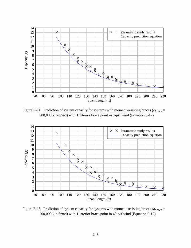
243
Figure E-14. Prediction of system capacity for systems with moment-resisting braces (kbrace =
200,000 kip-ft/rad) with 1 interior brace point in 0-psf wind (Equation 9-17)
Figure E-15. Prediction of system capacity for systems with moment-resisting braces (kbrace =
200,000 kip-ft/rad) with 1 interior brace point in 40-psf wind (Equation 9-17)
Span Length (ft)
Cap
acit
y (
g)
70 80 90 100 110 120 130 140 150 160 170 180 190 200 210 220
0
1
2
3
4
5
6
7
8
9
10
11
12
13
14
70 80 90 100 110 120 130 140 150 160 170 180 190 200 210 220
0
1
2
3
4
5
6
7
8
9
10
11
12
13
14
Parametric study results
Capacity prediction equation
Span Length (ft)
Cap
acit
y (
g)
70 80 90 100 110 120 130 140 150 160 170 180 190 200 210 220
0
1
2
3
4
5
6
7
8
9
10
11
12
13
14
70 80 90 100 110 120 130 140 150 160 170 180 190 200 210 220
0
1
2
3
4
5
6
7
8
9
10
11
12
13
14
Parametric study results
Capacity prediction equation
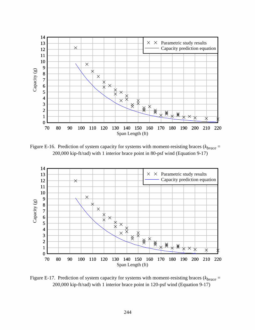
244
Figure E-16. Prediction of system capacity for systems with moment-resisting braces (kbrace =
200,000 kip-ft/rad) with 1 interior brace point in 80-psf wind (Equation 9-17)
Figure E-17. Prediction of system capacity for systems with moment-resisting braces (kbrace =
200,000 kip-ft/rad) with 1 interior brace point in 120-psf wind (Equation 9-17)
Span Length (ft)
Cap
acit
y (
g)
70 80 90 100 110 120 130 140 150 160 170 180 190 200 210 220
0
1
2
3
4
5
6
7
8
9
10
11
12
13
14
70 80 90 100 110 120 130 140 150 160 170 180 190 200 210 220
0
1
2
3
4
5
6
7
8
9
10
11
12
13
14
Parametric study results
Capacity prediction equation
Span Length (ft)
Cap
acit
y (
g)
70 80 90 100 110 120 130 140 150 160 170 180 190 200 210 220
0
1
2
3
4
5
6
7
8
9
10
11
12
13
14
70 80 90 100 110 120 130 140 150 160 170 180 190 200 210 220
0
1
2
3
4
5
6
7
8
9
10
11
12
13
14
Parametric study results
Capacity prediction equation
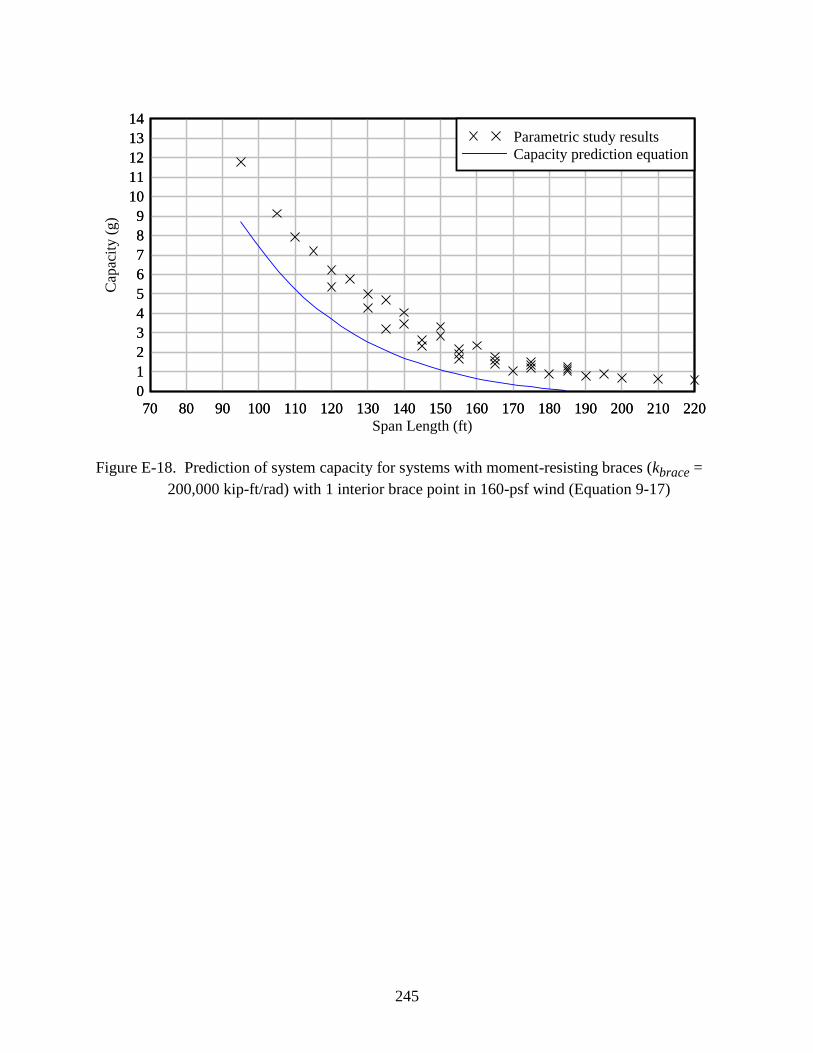
245
Figure E-18. Prediction of system capacity for systems with moment-resisting braces (kbrace =
200,000 kip-ft/rad) with 1 interior brace point in 160-psf wind (Equation 9-17)
Span Length (ft)
Cap
acit
y (
g)
70 80 90 100 110 120 130 140 150 160 170 180 190 200 210 220
0
1
2
3
4
5
6
7
8
9
10
11
12
13
14
70 80 90 100 110 120 130 140 150 160 170 180 190 200 210 220
0
1
2
3
4
5
6
7
8
9
10
11
12
13
14
Parametric study results
Capacity prediction equation

246
LIST OF REFERENCES
AASHTO (American Association of State Highway and Transportation Officials) (2010). LRFD
Bridge Design Specifications: 5th
Edition, AASHTO, Washington, D.C.
ADINA (2012). Theory and Modeling Guide, Volume 1: ADINA Solids & Structures, ADINA
R&D, Inc, Watertown, MA.
AF&PA (American Forest & Paper Association) (2005). National Design Specification for Wood
Construction and Supplement, AF&PA, Washington, D.C.
AIJ (Architectural Institute of Japan) (2004). AIJ Recommendations for Loads on Buildings, AIJ,
Tokyo.
ASCE (American Society of Civil Engineers) (2006). ASCE 7‒05: Minimum Design Loads for
Buildings and Other Structures, ASCE, New York, NY.
ASCE Wind Effects Committee (1987). Wind Loading and Wind-Induced Structural Response,
American Society of Civil Engineers, New York, NY.
Bathe, K. (1996). Finite Element Procedures, Prentice Hall, Englewood Cliffs, NJ.
Bradley, G. and Chang, P. (1998). Determination of the Ultimate Capacity of Elastomeric
Bearings Under Axial Load, NISTIR 6121, Building and Fire Research Laboratory,
Gaithersburg, MD.
BSI (British Standards Institution) (2006). BS 5400: Steel concrete and composite bridges: Part
2: Specification for loads, BSI, London.
CEN (European Committee for Standardization) (2004). Eurocode 1: Actions on Structures –
Part 1‒4: General Actions – Wind Actions (prEN 1991‒1‒4:2004), CEN, Brussels.
Çengel, Y. and Cimbala, J. (2006). Fluid Mechanics: Fundamentals and Applications, McGraw–
Hill Higher Education, Boston, MA.
Consolazio, G., Hamilton, H., and Berry, M. (2012). Experimental Validation Of Bracing
Recommendations For Long-Span Concrete Girders, Structures Research Report No.
2012/72909‒74040, University of Florida, Gainesville, FL.
Consolazio, G., Hamilton, H., Bui, L., and Chung, J. (2007). Lateral Bracing of Long-Span
Florida Bulb-Tee Girders, Structures Research Report No. 2007/52290, University of
Florida, Gainesville, FL.
Davenport, A. (1960). Wind Loads on Structures, Technical Paper No. 88, Division of Building
Research, Ottawa, Canada.
Delany, N. and Sorensen, N. (1953). Low Speed Drag of Cylinders of Various Shapes, Technical
Note 3038, National Advisory Committee for Aeronautics, Washington, D.C.
247
ESDU (1982). ESDU 82007: Structural Members: Mean Fluid Forces on Members of Various
Cross Sections, ESDU, London.
FDOT (Florida Department of Transportation) (2009). Temporary Design Bulletin C09‒07,
FDOT, Tallahassee, FL.
FDOT (Florida Department of Transportation) (2010). Standard Specifications for Road and
Bridge Construction, FDOT, Tallahassee, FL.
FDOT (Florida Department of Transportation) (2012a). Design Standard No. 20005: Prestressed
I-Beam Temporary Bracing, FDOT, Tallahassee, FL.
FDOT (Florida Department of Transportation) (2012b). Instructions for Design Standard No.
20010: Prestressed Florida-I Beams, FDOT, Tallahassee, FL.
FDOT (Florida Department of Transportation) (2012c). Design Standard No. 20510: Composite
Elastomeric Bearing Pads – Prestressed Florida-I Beams, FDOT, Tallahassee, FL.
FDOT (Florida Department of Transportation) (2012d). Instructions for Design Standard No.
20510: Composite Elastomeric Bearing Pads – Prestressed Florida-I Beams, FDOT,
Tallahassee, FL.
FDOT (Florida Department of Transportation) (2012e). Structures Manual Volume I: Structures
Design Guidelines, FDOT, Tallahassee, FL.
Gent, A. (2001). Engineering with Rubber: How to Design Rubber Components 2nd
Edition,
HanserGardner Publications Inc., Cincinnati, OH.
Grant, I. and Barnes, F. (1981). “The Vortex Shedding and Drag Associated with Structural
Elements”, Journal of Wind Engineering and Industrial Aerodynamics, Vol. 8, pp. 115–
122.
Haslach, H. and Armstrong, R. (2004). Deformable Bodies and their Material Behavior, John
Wiley & Sons, New York, NY.
Holmes, J. (2007). Wind Loading of Structures: 2nd
Edition, Taylor & Francis, New York, NY.
Kalkan, İ. (2010). “Application of Southwell Method on the Analysis of Lateral Torsional
Buckling Tests on Reinforced Concrete Beams”, International Journal of Engineering
Research & Development, Vol. 2, No. 1, pp. 58–66.
Mast, R. (1993). “Lateral Stability of Long Prestressed Concrete Beams – Part 2”, PCI Journal,
Vol. 38, No. 1, January–February 1993, pp. 70–88.
Maher, F. and Wittig, L. (1980). “Aerodynamic Response of Long H-Section”, Journal of the
Structural Division, ASCE, Vol. 106, No. ST1, pp. 183–198.

248
Mandal, P. and Calladine, C. (2002). “Lateral–Torsional Buckling of Beams and the Southwell
Plot”, International Journal of Mechanical Sciences, Vol 44, No. 12, pp. 2557–2571.
Massey, C. (1963). “Elastic and Inelastic Lateral Instability of I-Beams”, The Engineer, Vol.
216, No. 5622, pp. 672–674.
Meck, H. (1977). “Experimental Evaluation of Buckling Loads”, Journal of the Engineering
Mechanics Division, ASCE, Vol. 103, No. 2, pp. 331–337.
Myers, G. and Ghalib, A. (n.d.). “Wind Loads on Steel Box Girders During Construction Using
Computational Fluid Dynamic Analysis”, Atkins Technical Journal, Vol 7, No. 110, pp.
83–92.
NRC (National Research Council) (2005). User’s Guide – NBC 2005, Structural Commentaries,
NRC, Ottawa, Canada.
PCI (2010). PCI Design Handbook: 7th
Edition, Precast/Prestressed Concrete Institute, Chicago,
IL.
Podolny, W. and Muller, J. (1982). Construction and Design of Prestressed Concrete Segmental
Bridges, John Wiley & Sons, New York, NY.
Sachs, P. (1978). Wind Forces in Engineering: 2nd
Edition, Pergamon Press, Oxford.
Scruton, C. and Newberry, C. (1963). “On the Estimation of Wind Loads for Building and
Structural Design”, ICE Proceedings, Vol. 25, No. 2, June 1963, pp. 97–126.
Simiu, E. and Miyata, T. (2006). Design of Buildings and Bridges for Wind: A Practical Guide
for ASCE-7 Standard Users and Designers of Special Structures, John Wiley & Sons,
New York, NY.
Solari G. and Kareem A. (1998). “On the Formulation of ASCE 7‒95 Gust Effect Factor”,
Journal of Wind Engineering and Industrial Aerodynamics, Vol. 77, pp. 673–684.
Southwell, R. (1932). “On the Analysis of Experimental Observations in Problems of Elastic
Stability”, Proceedings of the Royal Society of London, Vol. 135, No. 828, pp. 601–616.
Stanton, J., Roeder, C., Mackenzie-Helnwein, P., White, C., Kuester, C., and Craig, B. (2008).
Rotation Limits for Elastomeric Bearings: Appendix F, NCHRP Report 596,
Transporation Research Board, National Research Council, Washington D.C.
Trahair, N. (1969). “Deformations of Geometrically Imperfect Beams”, Journal of the Structural
Division, ASCE, Vol. 95, No. ST7, pp. 1475–1496.
Treloar, L. (1975). The Physics of Rubber Elasticity: 3rd
Edition, Clarendon Press, Oxford.
Young, W. C. and Budynas, R. G. (2002). Roark’s Formulas for Stress and Strain: 7th
Edition,
McGraw–Hill, New York, NY.

249
BIOGRAPHICAL SKETCH
The author was born in Tallahassee, Florida, in 1986. He began attending the University
of Florida in August 2004, where he received the degree of Bachelor of Science in mechanical
engineering in May 2009. He then enrolled in graduate school at the University of Florida where
he received a Master of Science in civil engineering in May 2013, with an emphasis in civil
structures.