BRIDGE DESIGN FOR EARTHQUAKE FAULT CROSSINGS - SYNTHESIS ... · PDF fileBRIDGE DESIGN FOR...
139
BRIDGE DESIGN FOR EARTHQUAKE FAULT CROSSINGS: SYNTHESIS OF DESIGN ISSUES AND STRATEGIES A Thesis Presented to the Faculty of California Polytechnic State University San Luis Obispo In Partial Fulfillment of the Requirements for the Degree of Master of Science in Civil & Environmental Engineering By Osmar Rodriguez March, 2012
Transcript of BRIDGE DESIGN FOR EARTHQUAKE FAULT CROSSINGS - SYNTHESIS ... · PDF fileBRIDGE DESIGN FOR...

BRIDGE DESIGN FOR EARTHQUAKE FAULT CROSSINGS: SYNTHESIS OF DESIGN
ISSUES AND STRATEGIES
A Thesis
Presented to the Faculty of
California Polytechnic State University
San Luis Obispo
In Partial Fulfillment
of the Requirements for the Degree of
Master of Science in Civil & Environmental Engineering
By
Osmar Rodriguez
March, 2012

ii
© 2012
Osmar Rodriguez
ALL RIGHTS RESERVED

iii
COMMITTEE MEMBERSHIP
TITLE: Bridge Design for Earthquake Fault Crossings: Synthesis of
Design Issues and Strategies
AUTHOR: Osmar Rodriguez
DATE SUBMITTED: March, 2012
COMMITTEE CHAIR: Dr. Rakesh Goel, Civil & Environmental Engineering
Department Chair
COMMITTEE MEMBER: Dr. Bing Qu, Civil & Environmental Engineering
Assistant Professor
COMMITTEE MEMBER: Dr. Eric Kasper, Civil & Environmental Engineering
Assistant Professor

iv
ABSTRACT
Bridge Design for Earthquake Fault Crossings: Synthesis of Design Issues and Strategies
By Osmar Rodriguez
This research evaluates the seismic demands for a three-span curved bridge crossing fault rupture
zones. Two approximate procedures which have been proved adequate for ordinary straight
bridges crossing fault-rupture zones, i.e., the fault-rupture response spectrum analysis (FR-RSA)
procedure and the fault-rupture linear static analysis (FR-LSA) procedure, were considered in
this investigation. These two procedures estimate the seismic demands by superposing the peak
values of quasi-static and dynamic bridge responses. The peak quasi-static response in both
methods is computed by nonlinear static analysis of the bridge under the ground displacement
offset associated with fault-rupture. In FR-RSA and FR-LSA, the peak dynamic responses are
respectively estimated from combination of the peak modal responses using the complete-
quadratic-combination rule and the linear static analysis of the bridge under appropriate
equivalent seismic forces. The results from the two approximate procedures were compared to
those obtained from the nonlinear response history analysis (RHA) which is more rigorous but
may be too onerous for seismic demand evaluation. It is shown that the FR-RSA and FR-LSA
procedures which require less modeling and analysis efforts provide reasonable seismic demand
estimates for practical applications.

v
ACKNOWLEDGMENTS
It is a pleasure to thank Dr. Rakesh Goel for his support, supervision, and wisdom
throughout this entire process. Thanks to him and his acceptance onto this project, I have found
my strengths in seismic and structural engineering. I am thoroughly honored to have worked
under such direction and greatly respect your accomplishments and advancements in these fields.
I offer my sincerest gratitude to my assistant thesis advisor, Dr. Bing Qu, who has
supported me throughout this project with his knowledge, patience, and guidance. I attribute the
level of my master’s degree to his encouragement and effort and without him this thesis, too,
would not have been possible, thank you. To Dr. Eric Kasper for taking time out of his schedule
to take part in my thesis review committee and providing important advice on how to refine
certain aspects of my research. Also to all of my professors at Cal Poly who have inspired and
guided me through my college career.
To my colleagues Tòmas Bowdey, Colin Leung, Jacky Ng, and Rachel Goosens for
holding the utmost self-discipline while going through this program together. I look forward to
seeing what each of your careers and future bring. To my close friends who have been with me
from day one, I appreciate your patience and forbearance through all this; I could not have done
it without all of you teasing and pushing me daily to finish already.
To my girlfriend Alyssa who has been with me far before I became an engineering
master, thank you for everything you do and the person you are. Your ability to pretend to care
about or listen to me talk about any of these technical concepts without leaving me amazes me. I
am fortunate to have found someone as beautiful and caring as you.
To God, thank you for giving me strength to continue moving forward every day. Lastly,
to my mother and father for encouraging my sister and me to become anything we wanted and
supporting us whole-heartedly through our path there. For showing us what true hard work is and
how anything is obtainable through it, thank you. This thesis is dedicated to you.

vi
The research reported in this thesis is supported by CALTRANS under Contract No.
65A0379 with Dr. Allaoua Kartoum as the project manager. The support is gratefully
acknowledged. We acknowledge Drs. Tom Shantz and Brian Chiou from the Division of
Research and Innovation of CALTRANS who simulated the ground motions used in this
investigation. We are also grateful to Mark Yashinsky, Foued Zayati, Mark Mahan, and Toorak
Zokaie of CALTRANS for their useful feedback on this research investigation. Moreover, the
original finite element bridge model was developed by Dr. Farzin Zareian from University of
California at Irvine.

vii
TABLE OF CONTENTS
TABLE OF TABLES .................................................................................................................... x
TABLE OF FIGURES ................................................................................................................. xi
CHAPTER 1: STATEMENT OF RESEARCH ......................................................................... 1
1.1 Introduction ........................................................................................................................... 1
1.2 Current Problem .................................................................................................................... 2
1.2.1 Bolu Viaduct, Turkey – November 12th
, 1999 ............................................................... 2
1.2.2 Wenchuan, China – May 18th
, 2008 .............................................................................. 3
1.2.3 Denali, Alaska- November 3rd
, 2002 ............................................................................. 4
1.3 Previous Investigations ......................................................................................................... 5
1.4 Scope of Investigation........................................................................................................... 7
1.4.1 Phase 1: Identification of Bridge Examples................................................................... 7
1.4.2 Phase 2: Selection of Ground Motion Histories and Design Spectrum ......................... 9
1.4.3 Phase 3: Development of Computer Models ............................................................... 10
1.4.4 Phase 4: Evaluation of Previous Procedures ................................................................ 10
1.4.5 Phase 5: Evaluation of Analysis Procedures for Practical Use .................................... 11
CHAPTER 2: REVIEW OF EXISTING ANALYSIS METHODS ....................................... 12
2.1 Introduction ......................................................................................................................... 12
2.2 Existing Analysis Methods for Bridges Crossing Fault-Rupture Zones ............................. 12

viii
2.2.1 Theoretical Background: Linear Analysis ................................................................... 13
2.2.2 Nonlinear Response History Analysis ......................................................................... 15
2.2.3 Fault-Rupture Response Spectrum Analysis ............................................................... 16
2.2.4 Fault-Rupture Linear Static Analysis ........................................................................... 18
2.3 Extension of Previous Study ............................................................................................... 20
CHAPTER 3: GROUND MOTIONS ....................................................................................... 21
3.1 Introduction ......................................................................................................................... 21
3.2 Generation of Ground Motions ........................................................................................... 21
3.2.1 Selected Record Sets .................................................................................................... 22
3.2.2 Modification of Set Components ................................................................................. 23
3.3 Ground Motion Analysis..................................................................................................... 26
3.3.1 Spatially-Uniform Ground Motions ............................................................................. 27
3.3.2 Spatially-Varying Ground Motion Across Fault-Rupture Zones................................. 28
3.4 Development of CALTRANS Target Spectrum ................................................................. 28
CHAPTER 4: DEVELOPMENT OF COMPUTER MODEL .............................................. 31
4.1 Introduction ......................................................................................................................... 31
4.2 Bridge 55-0837S Information ............................................................................................. 32
4.3 Linear and Nonlinear Models of Bridge 55-0837S............................................................. 35
4.4 Model Components ............................................................................................................. 36

ix
4.4.1 Deck System ................................................................................................................ 37
4.4.2 Bent Supports ............................................................................................................... 38
4.4.3 Abutment Model Design .............................................................................................. 39
4.4.6 Zero-Length Members ................................................................................................. 42
4.5 Consideration of Bridge Orientations ................................................................................. 45
CHAPTER 5: RESULTS AND DISCUSSION ....................................................................... 47
5.1 Response Quantities of Interest .......................................................................................... 47
5.2 Results ................................................................................................................................. 48
5.3 Discussion of Results .......................................................................................................... 50
5.3.1 Abutments .................................................................................................................... 50
5.3.2 Bent Supports ............................................................................................................... 53
5.4.3 Accuracy of Procedures ............................................................................................... 55
CHAPTER 6: CONCLUSIONS & RECOMMENDATIONS ................................................ 57
CHAPTER 7: RECOMMENDATIONS FOR SUBSEQUENT STUDY ............................... 62
REFERENCES ............................................................................................................................ 63
APPENDICES ............................................................................................................................. 66
Appendix A: Ground Motion Summary…………………………………………………..…70
Appendix B: Mode Shapes and Periods……………………………………………………..92
Appendix C: Complete Result Comparisons of Bridge 55-0837S…………………………111

x
TABLE OF TABLES
Table 1. Summary of considered base ground motion pairs ......................................................... 22
Table 2. Summary of deck system properties for deck elements 1-30 ......................................... 38
Table 3. Finite Element Model Zero-length member summary ................................................ 44

xi
TABLE OF FIGURES
Figure 1. Damage at western abutment of Bolu Viaduct, deck displacement due to support
failure (Ghasemi 2004) ................................................................................................................... 3
Figure 2. Full bridge collapse due to Wenchuan earthquake (Kawashima et al. 2008) ................. 4
Figure 3. Seismic support system along oil pipeline (Honegger et al. 2004) ................................. 5
Figure 4. Bridge 55-0837S (a) plan view and (b) elevation view ................................................... 9
Figure 5. Sketch of the effective influence vector for a bridge crossing fault rupture zones ....... 19
Figure 6. Example acceleration pulse that was added to Record Set 1 to create a 50 cm fling
step (Shantz and Chiou 2010) ....................................................................................................... 24
Figure 7. Example acceleration pulse that was added to Record Set 1 to create a 50 cm fling step
(Shantz and Chiou 2010) .............................................................................................................. 25
Figure 8. Time histories for (a) Rec1_BN90 and (b) Rec1_BP90 ................................................ 26
Figure 9. CALTRANS design spectrum plotted against 10 record sets (a) and against the
mean of their geometric means (b) ............................................................................................... 30
Figure 10. Plan and elevation views of Bridge 55-0837S ............................................................ 32
Figure 11. Schematic of Bridge 55-0837S .................................................................................... 33
Figure 12. Single box girder typical section for Bridge 55-0837S ............................................... 34
Figure 13. Bent support cross-sections for Bridge 55-0837S ....................................................... 34
Figure 14. Bent support foundation typical section for Bridge 55-0837S .................................... 35
Figure 15. Assignments of nodes and elements in plan view for the FE model of Bridge 55-
0837S ............................................................................................................................................ 37

xii
Figure 16. Assignments of nodes and elements in elevation view for the FE model of Bridge
55-0837S ....................................................................................................................................... 39
Figure 17. Simplification of longitudinal abutment springs ......................................................... 41
Figure 18. Actual bent support cross-section (a) and expected inelastic regions at bent support
(b) .................................................................................................................................................. 43
Figure 19. Location of zero-length member to a beam-column element ...................................... 44
Figure 20. Definition of bridge orientation angle ......................................................................... 46
Figure 21. Bridge orientation limit definitions ............................................................................. 46
Figure 22. Results for = 0 degrees and longitudinal abutment stiffness = 0.10Keff ................... 49
Figure 23. Results for = 0 degrees and longitudinal abutment stiffness = 0.55Keff ................... 49
Figure 24. Results for = 0 degrees and longitudinal abutment stiffness = 1.00Keff ................... 50
Figure 25. Accuracy of FR-RSA for abutments in transverse direction at all orientations using
both GM and DS for longitudinal abutment stiffness = 1.00Keff .................................................. 51
Figure 26. Accuracy of FR-RSA for abutments in longitudinal directions at all orientations
using both GM and DS for longitudinal abutment stiffness = 1.00Keff ........................................ 52
Figure 27. Accuracy of FR-LSA for abutments in transverse directions at all orientations
using both GM and DS for longitudinal abutment stiffness = 1.00Keff ........................................ 52
Figure 28. Accuracy of FR-LSA for abutments in longitudinal directions at all orientations
using both GM and DS for longitudinal abutment stiffness = 1.00Keff ........................................ 53
Figure 29. Accuracy of FR-RSA for bents at all orientations using both GM and DS for
longitudinal abutment stiffness = 1.00Keff .................................................................................... 54

xiii
Figure 30. Accuracy of FR-LSA for bents at all orientations using both GM and DS for
longitudinal abutment stiffness = 1.00Keff` ................................................................................... 54

1
CHAPTER 1: STATEMENT OF RESEARCH
1.1 Introduction
In response to the damage recently sustained by California bridges during recent earthquakes,
the California Department of Transportation (Caltrans) has taken extensive measures to update
seismic design procedures to more efficiently analyze bridges crossing fault lines. Currently
there are over 13,000 bridges in California, including roughly 120 of them crossing fault-rupture
zones or lying in very close proximity to them, therefore developing a more efficient and
convenient procedure to analyze such cases has become crucial. Currently the most arduous yet
most accurate method of analyzing seismic demands of bridges requires nonlinear response
history analysis (RHA) in which dynamic support motions from spatially varying ground
motions due to surface rupture are taken into account.
The investigation proposes to synthesize Caltrans’s current design issues in procedures
analyzing bridge structures near fault-rupture zones and provides measurements to overcome
such issues. This thesis focuses on evaluation of the adequacy of two simplified analysis
procedures developed and validated from by Goel and Chopra (Goel and Chopra 2008a, 2008b,
2009a, 2009b) i.e., (1) Fault-Rupture Linear Static Analysis (FR-LSA), and (2) Fault-Rupture
Response Spectrum Analysis (FR-RSA) methods in estimating the seismic demands of a three-
span curved bridge crossing a fault-rupture zone. Results from the simplified procedures were
compared to the “exact” seismic demands produced from nonlinear RHA. By proving that new,
more simplified methods of analysis are able to provide accurate displacement estimates, current

2
design and analysis measures are able to be updated and provide a faster approach for bridge
engineers to use.
The two presented procedures estimate the seismic demands on a bridge crossing earthquake
fault by superposing the peak values of quasi-static and dynamic bridge responses. The peak
quasi-static response in both methods is computed by nonlinear static analysis of the bridge
under the ground displacement offset associated with fault rupture. In FR-RSA and FR-LSA, the
peak dynamic responses are, respectively, estimated from combination of the peak modal
responses using the complete-quadratic-combination (CQC) rule and linear static analysis of the
bridge under appropriate equivalent seismic forces.
1.2 Current Problem
Although avoiding building bridges across fault lines all-together might be the best approach,
such situations are not always permissible. Regions of high seismicity such as in California leave
engineers without many options in design but instead create a great need for sound design over
such cases. Recent earthquakes have shown the prodigious vulnerability of bridges crossing
fault-rupture zones leaving them either damaged or in some cases fully collapsed. The following
sections briefly review the damages of such bridges observed from previous earthquakes.
1.2.1 Bolu Viaduct, Turkey – November 12th, 1999
For example, spans of the newly-constructed Bolu viaduct along the trans-European
expressway in Turkey were inches away from collapse in 1999 due to the fault movement along
the transverse direction of the bridge. According to seismologists, the rupture on November 12,
1999 was caused by a strike-slip rupture along the secondary Duzce fault with a magnitude of

3
7.2 with an epicenter located very close to the Bolu viaduct (Ghasemi 2004). The viaduct design
included a hybrid isolation system which suffered complete failure and narrowly avoided total
collapse due to excessive superstructure movement. The surface fault-rupture produced major
propagation between segments of the viaducts piers and decks, as shown in Figure 1. The
response of the Bolu Viaduct highlighted the importance of designing for high ground
movement, especially for structures near active fault zones.
Figure 1. Damage at western abutment of Bolu Viaduct, deck displacement due to support failure
(Ghasemi 2004)
1.2.2 Wenchuan, China – May 18th, 2008
Recent earthquakes in Wenchuan, China severely damaged bridges located near active fault
zones. While damage to bridges varied, several cases of full collapse were reported for bridges
on top of the actual fault, as shown in Figure 2. The significant ground offsets caused extensive
movement along the transverse direction of most of the bridges, leading to detachment of lateral
beams from columns at the joints. It was noted that major dislocation of the bridges members

4
occurred for curved bridges due to insufficient seismic design force and lack of ductility capacity
(Kawashima et al. 2008). Other major damages to bridges included; absence of unseating
prevention devices, bridge location crossing fault displacements, slope failures, and unreinforced
stone masonry bridges. The damage done along main roads resulted in navigation obstacles for
rescue teams and local rescue teams while damage done to local ordinary bridges produced
heavy complications for evacuation of local citizens.
Figure 2. Full bridge collapse due to Wenchuan earthquake (Kawashima et al. 2008)
1.2.3 Denali, Alaska- November 3rd, 2002
It has been shown that sound design of bridge structures across active fault lines is not only
possible but critical as well, as evident in the most recent earthquake occurring near the Denali
fault in Alaska in which key segments of the trans-Alaska oil pipeline survived from a right-
lateral strike-slip event. The lines held up against strike-lateral fault displacements caused by a
7.9 magnitude earthquake without any failures or leakage due to having proper seismic damage
prevention systems as shown in Figure 3 (Honegger et al. 2004). Aside from the main shock, the

5
Alaska Earthquake Information Center (AEIC) located over 35,000 aftershocks through the end
of 2004 of which the structure withstood without serious damage. The near-source motions
coupled with soil liquefaction developed significant bending and axial strain in the pipeline. The
structure resisted the ground motions in a manner consistent with the original design premise,
which allowed limited damage to the pipeline, support system (Nyman et al. 2006).
Figure 3. Seismic support system along oil pipeline (Honegger et al. 2004)
1.3 Previous Investigations
Classifications of bridges in California include both “lifeline” routes and “ordinary” bridges,
whose designs are governed by CALTRANS Seismic Design Criteria (SDC)(CALTRANS
2010). While site-specific seismological studies to define spatially varying ground motions and
rigorous nonlinear response history analysis (RHA) are necessary for important bridges on
“lifeline” routes, such investigations may be too onerous for “ordinary” bridges. Seeing how a
large amount of California’s bridges are classified as “ordinary”, the investigation proposes the

6
validity behind simplified procedures to fill the need for providing accurate estimation of seismic
demands and facilitate evaluation and design of such “ordinary” bridge scenarios.
In a previous investigation, Goel and Chopra (2008a) developed simplified procedures to
analyze and compare seismic performance of bridges subjected to fault offset displacement and
ground shaking. However, due to limited scope of the investigation, applicability of these
procedures was demonstrated for idealized straight ordinary bridge models. Based on Goel and
Chopra (2008a), this investigation extends the methods of approximation to actual curved
bridges.
A comprehensive study by Afshin and Amjadian (2010) illustrated that bridges with complex
geometries such as curved bridges are more susceptible to seismic damage than straight highway
bridges with regular geometry. The study showed that coupling of translational and rotational
movements of the deck effectively produce striking effects on the concrete catalyzing for
possible deck or support rupture. Afshin and Amjadian (2010) modeled the deck of the
superstructure as being dynamic in-plane, however with material properties remaining intact and
linear during earthquake excitation, demonstrating normal behaviors unless under an irregularly
large quake. The reinforced-concrete bent supports were modeled with rigid constraints and
nodal mass elements that include the rotary mass of the support in three orthogonal directions
(Ingham et al. 1997).
Tseng and Penzien (1975) produced a study of the coupled inelastic flexural behavior of bent
supports by using a three-dimensional elastoplastic model, and the discontinuous behavior
commonly seen in expansion joints by a nonlinear model used in this study (Chen 2001). In their

7
model, important nonlinear characteristics such as effects of separation, impact, and slippage of
soil-abutment interfaces were all implemented and accounted for. Since then, contributions to the
development of nonlinear models for bridges have advanced greatly. Toki (1980) contributed to
the implementation of nonlinear responses of continuous bridges subjected to traveling seismic
waves, which is fully used in this investigation. Ghusn and Saiidi (1986) used bilinear biaxial
bending elements (a five-spring system) for the interaction between pier columns and soil.
Imbsen and Penzien (1986) considered the evaluation of energy-absorption characteristics of
highway bridges including kinematic hardening features through the design of nonlinear beam-
column elements for pier columns.
1.4 Scope of Investigation
In order to complete the work in a timely and logical manner, the research was broken down
into the following phases:
1.4.1 Phase 1: Identification of Bridge Examples
A total of six existing bridge models crossing fault-rupture zones have been provided by
Caltrans to for research. These bridges have been analyzed by researchers from the University of
California, Irvine for other research purposes. The bridges included:
(1) Bridge 29-0315K – Jacktone SB99 On-Ramp Separation
(2) Bridge 29-0318 – Jacktone Road OH
(3) Bridge 53-2883S – Carson St – N605 Ramp
(4) Bridge 55-0837S - West Street – N5 On-Ramp
(5) Bridge 55-0938 - La Veta Ave. OC

8
(6) Bridge 55-0939G - E22-N55 Connector
All bridges have been reviewed to be suitable to fit parameters needed for evaluation, including
being three or four spans, with single or multi-column bents, and being skewed or curved. After
detailed comparisons of all six bridges, Bridge 55-0837S (4) which is a three-span curved bridge
built in 2000 located in east Anaheim, California (District 12 – Orange County), and serves as
the West Street to Northbound 5 Interstate on-ramp was chosen to serve as the principal structure
for investigation. The West Street Bridge serves greatly as a main on-ramp for large groups of
vehicles leaving Disneyland, one of the world’s most visited attractions. It holds routes both on
the deck of the structure and has a crossing route under the structure. The bridge itself crosses
over eight lanes of high density traffic routes, four heading south, and four heading north on
Interstate-5 with a vertical clearance of 18.5 ft. Figure 4 (a) and (b) provide plan view and
elevation of the selected bridge. Being a three-span, curved bridge, without skew or base
isolation systems, Bridge 55-0837S served naturally as a proper scenario under the scope of this
thesis.
(a)

9
(b)
Figure 4. Bridge 55-0837S (a) plan view and (b) elevation view
1.4.2 Phase 2: Selection of Ground Motion Histories and Design Spectrum
As previously mentioned, nonlinear RHA provides an “exact” approach for dynamic analysis
of a structural model in a seismic design process. Theory rooted in the nonlinear analysis creates
a heightened sensitivity to effects of ground acceleration records being used, making selection of
them critical. Previous research done at University California at Berkeley provided ground
motion time histories from direct simulation using simplified earth structure and rupture history
for each set (Dreger et al. 2007). However for the evaluation at hand, the more desirable
approach was use actual recorded motions, scaled for relative source size, and spectral
characteristics which will be gone into more detail later. In order to provide a more appropriate
scenario of bridges being placed directly atop of fault crossings, ground motions running at a
very close proximity to bridge supports were selected, simulated, and analyzed.
Using the Next Generation Attenuation (NGA) database, Caltrans has provided a set of 10
ground motion record sets at which levels of intensity, severity, time step, and location vary.
Record sets were filtered to match design criteria set by Caltrans bridge engineers. A design

10
spectrum was then produced from the mean of the geometric means of the 10 ground motion
record sets to be used to compare its accuracy in representing the total set during analysis.
1.4.3 Phase 3: Development of Computer Models
The general computational approach of this investigation was to model the structure from the
supporting soils up to the superstructure, apply prescribed earthquake displacements, and solve
the equations of motion using three different methods to calculate the bridge’s structural
response and evaluate the effectiveness of each procedure.
The finite element bridge model developed in Open System for Earthquake Engineering
Simulation (OpenSees) (Mazzoni et al. 2006) by the researches from the University of
California, Irvine was modified into both linear elastic and nonlinear inelastic models for use in
this investigation. Spring systems were assigned to both bent supports and abutments to consider
soil structure interactions. Restraining effects due to presence of shear keys, wing walls, and
back walls at abutments were also considered in defining spring stiffnesses in each direction.
1.4.4 Phase 4: Evaluation of Previous Procedures
The Fault-Rupture Linear Static Analysis (FR-LSA) and Fault-Rupture Response Spectrum
Analysis (FR-RSA) procedures had been previously developed by Goel and Chopra (2008a) and
validated for simple straight bridge models. As explained by Filippou (1992) the dynamically-
induced bending moments, shear forces, torsional moments and axial forces are calculated from
the modal displacements and stiffness properties of each bridge element. From this theory,
computation of vibration member forces is found using vibration displacements, while the
dynamic plus quasi-static displacements are utilized for calculating the total member forces. The

11
peak quasi-static response in both methods is computed by nonlinear static analysis of the bridge
underground displacement offset associated with fault-rupture. In FR-RSA and FR-LSA, the
peak dynamic responses are respectively estimated from combination of the peak modal
responses using the complete-quadratic-combination rule and linear static analysis of the bridge
under appropriate equivalent seismic forces. In the previous investigation by Goel and Chopra
(2008a), the procedures being analyzed primarily focused on fault-parallel components, which
differ from the current analysis where both fault-parallel and fault-normal components are
examined. Both methods were evaluated for accuracy in estimation in comparison to the “exact”
nonlinear RHA.
1.4.5 Phase 5: Evaluation of Analysis Procedures for Practical Use
The investigation focuses on providing valid and efficient procedures for bridge engineers to
implement into design and analysis standards. Ability of methods to adapt to variability in
bridge-to-fault orientation and longitudinal stiffness are appraised. Procedures are evaluated and
determined if suitable for implementation into design standards and structural analysis software.

12
CHAPTER 2: REVIEW OF EXISTING ANALYSIS
METHODS
2.1 Introduction
The general computational approach to the current investigation is to model the selected
three-span curved bridge from the foundation up to the superstructure, apply prescribed
earthquake displacements, and solve the equations of motion to calculate the structures seismic
response. The following sections review past, current, and state-of-the-art investigations
regarding bridges crossing high seismic fault zones. Goel and Chopra (2008a) have developed
and validated simplified analysis procedures for idealized ordinary straight bridges crossing
fault-rupture zones. A main purpose of this research is to extend the theories evaluated in these
prior investigations to actual curved bridges.
2.2 Existing Analysis Methods for Bridges Crossing Fault-Rupture Zones
As presented by the comprehensive research report by Goel and Chopra (2008a), two
simplified analysis methods, i.e., FR-LSA and FR-RSA were developed for bridges crossing
fault lines. As alternatives to the nonlinear RHA approach, the simplified methods provide
predictions of seismic displacement demands. The methods were developed to provide viable
peak responses of linearly-elastic “ordinary” bridges for bridge engineers to use in avoidance of
the more rigorous nonlinear procedure of response history analysis (RHA). The study was
performed with a series of three companion journal papers (Goel and Chopra 2008a, 2008b,
2009a, 2009b) analyzing both linear-elastic and linear-inelastic bridge models. .

13
2.2.1 Theoretical Background: Linear Analysis
Both FR-RSA and FR-LSA procedures use superposition of peak values from quasi-static
( )s
ou and dynamic parts ( )ou , to form a total system response ( )tu for simple straight bridge
models. Both components ( )s
ou and ( )ou , are respectively found through: (1) static analysis of
the nonlinear bridge model with the peak values of all support displacements Equation (2.1) and
(2.2) applied simultaneously; and (2) conducting either the FR-RSA or FR-LSA procedures on
the linear bridge model under the fault-normal and fault-parallel ground motion components.
The presented linear analysis procedures use both general multiple-support excitation and
proportional multiple-support excitation theories to produce a total peak structural response. The
displacement components at support l of a bridge due to fault-rupture motion along the fault-
parallel and fault-normal directions,FP ( )glu t and
FN ( )glu t , may be respectively approximated as:
FP FP FP( ) ( )gl l gu t u t (2.1)
FN FN FN( ) ( )gl l gu t u t
(2.2)
where FP( )gu t and
FN ( )gu t are the fault-parallel and fault-normal displacement histories of
motion at a reference location, and where FPl and FN
l are the proportionality constants for the
thl support. For a bridge crossing strike-slip fault, FPl will be equal to +1 for supports on left
side of the fault and -1 for supports on right side of the fault, and FNl will be equal to +1 for

14
supports on both side of the fault. For bridges crossing other types of faults, i.e., faults with
other dip and rake angles, values of FPl and FN
l may differ from +1 or -1.
For ground excitations defined by Equations (2.1) and (2.2), the equations of motion are
demonstrated in Equation (2.3):
FP FP FN FNeff eff( ) ( )g gu t u t mu + cu + ku m m
(2.3)
where m , c , and k respectively represent the mass, stiffness and damping matrices of the
system; u , u and u respectively represent the acceleration, velocity, and displacement vectors
of the bridge; FPeff is the “effective” influence vector for fault-parallel motion defined as the
vector of displacements at all structural degrees of freedom due to simultaneous static
application of all support displacements with value equal to FPl at the thl support of the elastic
bridge model, FNeff is the “effective” influence vector for fault-normal motion defined as the
vector of displacements at all structural degrees of freedom due to simultaneous static
application of all support displacements with value equal to FNl at the thl support of the elastic
bridge model, and FP ( )gu t and
FN ( )gu t are the accelerations at the reference support in the fault-
parallel and fault-normal directions, respectively.
The total displacements of the bridge are then given by
FP FP FN FNeff eff( ) ( )g gu t u t mu + cu + ku m m (2.4)

15
FP FP FN FN FP FP FN FNeff eff
1 1
( ) ( ) ( ) ( ) ( ) ( ) ( )N N
t sg g n n n n n n
n n
t t t u t u t D t D t
u u u ι ι (2.5)
in which
FPeffFP
Tn
n Tn n
m
m
(2.6)
FNeffFN
Tn
n Tn n
m
m
(2.7)
and where FP( )nD t and FN ( )nD t are the deformation responses of the thn -mode SDF system
subjected to the reference ground motions FP ( )gu t and
FN ( )gu t in the fault-parallel and fault-
normal directions, respectively. The first two terms on right side of Equation (2.5) are the quasi-
static response and the last two terms are the dynamic response due to fault-parallel and fault-
normal support motions.
The following sections review previous procedures and assumptions for nonlinear RHA, FR-
RSA, and FR-LSA.
2.2.2 Nonlinear Response History Analysis
As previously mentioned, the main target of this investigation is to compare the results
produced from FR-RSA and FR-LSA to those calculated by the more rigorous nonlinear RHA.
The parametric study included ten sets of ground motion pairs and a design spectrum proposing
to accurately represent these sets, as described in detail in Chapter 3, being used as structural
excitations while holding the bridge model properties constant per set. RHA is recognized by

16
structural engineers to be the most precise in analyzing seismic demands of a structure and is
used to generate the “exact” seismic response. It is recognized that while the nonlinear RHA
method provides the most accurate results, such an analysis typically requires extensive
modeling and computational efforts, which many times is deemed too onerous for common
“ordinary” bridges crossing fault zones.
2.2.3 Fault-Rupture Response Spectrum Analysis
There are computational advantages in using FR-RSA for prediction of displacement
demands in structural systems. The FR-RSA procedure combines the responses of the bridge
caused by the fault offset and ground motions, which are respectively determined from the
nonlinear static analysis and the response spectrum analysis. The structures displacement caused
from this fault offset is created from longitudinal and/or the transverse vector components of the
fault offset (called the Design Fault Offset) based on the larger of the probabilistic and
deterministic offset.
Proportionality constants FPl and FN
l , and peak displacements at reference support location
of the bridge FPgou and
FNgou are found and applied to bent supports when forming the quasi-static
response of the structure. This quasi-static response is found through static analysis performed on
the nonlinear bridge model with fault offsets FP FPl gou and
FN FNl gou applied at support l in fault-
parallel and fault-normal directions, respectively. Note that FPgou and
FNgou may have both x- and
y-components depending on the angle between the bridge primary axis and the fault.

17
The peak dynamic responses, FPor and FN
or , of the linear elastic bridge due to fault-parallel
and fault-normal ground hazard are computed as follows:
1. Compute the vibration periods ( nT ) and mode shapes ( n ) of the bridge. Compute as
many modes as necessary to capture dynamic response of the bridge. In general, the first
18 to 24 modes were found to be sufficient in the example structures considered in this
study. A complete set of the bridges modes can be found in Appendix B.
2. Compute the fault rupture effective influence vectors, FPeff and FN
eff , as vectors of
displacements at all structural degrees of freedom due to simultaneous static application
of all support displacements with values equal to FPl and FN
l at the thl support.
3. Compute the modal participation factors for fault-parallel and fault-normal analysis as
FP FPeff
T Tn n n n m m and
FN FNeff
T Tn n n n m m . Note that these modal participation
factors differ from those in standard modal analysis to uniform support excitation.
4. Compute the response due to nth mode, FPnr and FN
nr , due to fault-parallel and fault-
normal ground hazards using modal analysis and modal participation factors computed in
last step.
5. Combine the modal responses, FPnr and FN
nr , due to fault-parallel and fault-normal
ground hazards using CQC procedure to obtain peak dynamic responses, FPor and FN
or ,
due to fault-parallel and fault-normal ground hazards, respectively.
This quasi-static responses FPQSr and FN
QSr , and the dynamic responses FPor and FN
or , are then
combined through Equation (2.8) to form a total structural response, t
or .
FP FN FP FNQS QS o o
tor r r r r (2.8)

18
The Complete Quadratic Combination (CQC) rule is used to combine the peak modal
response quantities caused from both fault-normal and fault-parallel ground motion components.
As seen in the procedure, modifications from using the standard RSA procedure were taken into
account to deal with actual fault-ruptured zones. By using both the modal participation factor, n
, and an “effective” influence vector, eff , all of the structures significant modes were able to be
evaluated. A complete set of the bridges mode shapes and periods can be found in Appendix B.
2.2.4 Fault-Rupture Linear Static Analysis
Goel and Chopra (2008a) evaluated the adequacy of FR-LSA to estimate seismic demands of
idealized straight bridges crossing fault-rupture zones. Identical to the FR-RSA procedure, FR-
LSA estimates the bridge peak response by superposing peak values from quasi-static and
dynamic responses. While calculation of the quasi-static response is equal in both procedures
they differ in calculating a dynamic response. As presented in the FR-RSA procedure, the quasi-
static response is found through static analysis performed on the nonlinear bridge model with
fault offsets FP FPl gou and
FN FNl gou applied at support l in fault-parallel and fault-normal
directions, respectively.
FR-LSA was developed through simplifying the FR-RSA procedure by recognizing that the
spectral acceleration associated with the periods of the considered modes may be conservatively
approximated to be a value equal to 2.5 times the peak ground acceleration (Goel and Chopra
2008a). Such a simplification avoids calculation of the bridge’s vibrational period, making it
significantly easier and practical for bridge engineers to use. The following steps have been

19
provided by Goel and Chopra (2008a) and are applied to the bridge structure to compute the
dynamic response, or , in FR-LSA:
(1) Compute effective influence vector eff , as shown in Figure 5, as the vector of
displacements in the structural DOF obtained by static analysis of the bridge due to
support displacements determined from Equation (2.1) and (2.2) applied simultaneously.
Figure 5. Sketch of the effective influence vector for a bridge crossing fault rupture zones
(2) Compute the dynamic response or by static analysis of the bridge due to lateral forces
2.5 eff gom u .
A final peak response is then calculated through which both the quasi-static response ( )QS
or
from the fault offset in the nonlinear model and the ground motion combination response
. .( )FN i FP i
o or r from the fault-normal and fault-parallel ground motions in the linear model are
combined as shown in Equation (2.9):
. .max ( = 1 or 2; = 1 or 2)t QS FN i FP j
o o o or r r r i j (2.9)
where:
(1) .1
_ _ caused by 2.5FN
o eff FN go FNr m u

20
(2) .1
_ _ caused by 2.5FP
o eff FP go FPr m u
(3) .2
_ _ caused by -2.5FN
o eff FN go FNr m u
(4) .2
_ _ caused by -2.5FP
o eff FP go FPr m u
and m represents the mass matrix in the equation of motion; _eff FP and
_eff FP represent the
effective influence vectors for fault-normal and fault-parallel motions; and _go FNu and
_go FPu
respectively represent the peak ground accelerations of the fault-normal and fault-parallel
motions.
2.3 Extension of Previous Study
It must be noted that the structural systems considered in the investigation provided by Goel
and Chopra (2008a) included: (1) a three-span symmetric bridge; (2) a three-span unsymmetric
bridge; (3) a four-span symmetric bridge; and (4) a four-span unsymmetric bridge. Each of the
bridge models were modeled as being “ordinary” straight bridges with the fault crossing between
bent supports and for all bridges, and each of the bent supports modeled as being fixed
(restrained in all six degrees-of-freedom). Results of the parametric study successfully provided
“accurate” estimates of bridge displacements using all three analysis methods with varying levels
of acceptable precision. This thesis will fill the need of extending these procedures and
evaluating them to a real bridge model of an existing curved, three-span bridge with variability in
bridge-fault orientations.

21
CHAPTER 3: GROUND MOTIONS
3.1 Introduction
Theory rooted in all three RHA, FR-RSA, and FR-LSA procedures makes selection of
appropriate ground excitations critical. Several ground motion records were required to prove the
adequacy of the analysis methods in extending to varying excitation levels and motion variables.
The ground motions used in this thesis were generated and provided by Caltrans in both Bridge-
Normal (BN) and Bridge-Parallel (BP) directions in order to simulate fault-rupture occurring
between bents. The following sections describe the generation and analysis of ground motions as
well as the development of the CALTRANS target spectrum.
3.2 Generation of Ground Motions
Ground motion pairs were selected to match the design spectrum provided by CALTRANS
Seismic Design Criteria (CALTRANS 2010). Using the Next Generation Attenuation (NGA)
database, record pairs were filtered to match the following requested CALTRANS criteria:
(1) Records must be from either free-field seismometers or nodes located in the bottom story
of a light frame structure.
(2) The lowest usable frequency of either record must be less than or equal to 0.2 Hz (as
specified in the NGA dataset.
(3) The event magnitude must fall within a range of 6.6 to 7.1.
(4) Records must be from sites no closer than 20 km from the rupturing fault. This
requirement was added so that the records would have minimum directivity effect in their
signal before the addition of the fling step.

22
The record sets chosen were developed from base record pairs that have been amplitude
scaled and modified by acceleration pulse. Once integrated into a displacement waveform, the
acceleration pulse includes a quasi-static displacement step which represents a specific fault
offset also known as a “fling step”. A relative fault offset of 100 cm was found to place bridge
bents into the inelastic range while not dominating the contribution of the dynamic response
(Shantz and Chiou 2010).
3.2.1 Selected Record Sets
Due to the limited number of actual ground motions recorded very close to actual ruptured
faults (less than 100 m) ground motion simulations are the only method to obtain time histories
for structural analysis. These simulated time histories are required to incorporate the near-fault
source radiation pattern, and account for far-and near-field seismic radiation during rupture
process as well as the sudden elastic rebound (Shantz and Chiou 2010). In total, 200 records
were provided by CALTRANS: (10 record sets) x (4 orientations + 1 no fling record) x (2
components) x (left or right side of fault) = 200. The actual final use of the four orientation sets
and left and right components are discussed in detail in the following section. Table 1 lists the
recorded ground motions that were used for generation of fault rupture ground motions and
illustrates the varying levels of intensity, severity, time step, and location.
Table 1. Summary of considered base ground motion pairs*
Set No. Component 1 Component 2 Time step (sec) Number of Points
1 LOMAP-BVC220 LOMAP-BVC310 0.005 5918
2 LOMAP-HSP000 LOMAP-HSP090 0.005 11990
3 LOMAP-HDA165 LOMAP-HDA255 0.005 7928
4 KOBE-FUK000 KOBE-FUK090 0.02 3900
5 NORTHR-SAR000 NORTHR-SAR270 0.01 3600
6 NORTHR-NEE090 NORTHR-NEE180 0.01 4800
7 KOBE-OSA000 KOBE-OSA090 0.02 6000

23
8 KOBE-ABN000 KOBE-ABN090 0.01 14000
9 ITALY-A-TDG000 ITALY-A-TDG270 0.0029 18216
10 SFERN-WND143 SFERN-WND233 0.001 7997 *selected from the NGA database.
Additional selection considerations included choosing record pairs with minimal scale factors
in order to avoid excessive amounts of actual manipulation of amplitudes. The greatest of the 10
record sets scale factors being Record Set No. 4 – Kobe Earthquake with a scaling factor of
13.02.
3.2.2 Modification of Set Components
Problems arose in CALTRANS’ attempt to use a functional form for the slip velocity to
define the fling step (differentiating the function to acceleration) developed in Dreger (2007).
Properties of the functional form resulted in two related and undesirable properties:
(1) A high acceleration spike (approximately 1.5g) at the beginning of the pulse
(2) The acceleration spike resulted in drift when integrated to displacement, presumably due
to round-off error. Furthermore, the drift was difficult to remove, presumably due to
irregularity related to round-off error.
To avoid these problems, CALTRANS used a functional form of a sine wave to allow for
stableness under integration without a drift correction. As represented in Figure 6, the new
functional form was used to add a 50 cm fling step to each of the record sets.

24
Figure 6. Example acceleration pulse that was added to Record Set 1 to create a 50 cm fling step
(Shantz and Chiou 2010)
Rise time for the rate of displacement offset was modeled by CALTRANS as a log-normally
distributed random variable with mean calculated in Dreger (2007) where the rise time was
related to the acceleration pulse period as 0.60rise plseT T (Shantz and Chiou 2010). This
relationship accounted for initial and final portions of the displacement step relative to the stress
drop ( 0.4LN ) varying at a slower pace relative to the middle portion of the step. By doing so
a final relation between the periods and fault offset was able to be defined, as illustrated in
Figure 7.

25
Figure 7. Example acceleration pulse that was added to Record Set 1 to create a 50 cm fling step
(Shantz and Chiou 2010)
Uncertainty in S-wave arrival time in relationship to fault rupture velocity was accounted to
by CALTRANS in determining when to add the fling step. This relation was estimated by
adding a uniformly distributed random variable ranging from 0.65 to 2.8 seconds to the S-wave
arrival time to account for the fact that the faults rupture velocity was seen to be 20% slower than
the S-wave velocity (Shantz and Chiou 2010). The range from 0.65 to 2.8 seconds accounts for
the distance between the hypocenter and the bridge along the fault length not matching up, thus
having a time difference in arrival.
All record sets have been provided in bridge-normal (transverse) and bridge-parallel
(longitudinal) orientations, and further broken down to being on the left side or right side of fault
location, e.g. Rec1_BN90_left, Rec1_BN90_right, Rec1_BP90_left, and Rec1_BP90_right. Since
the fault-parallel component of shaking is of opposite polarity on each side of the fault, the
ground motions, when rotated back to bridge-normal (BN) and bridge-parallel (BP) orientations,
are different depending on whether a location is on the left side or right side of the fault (Shantz
and Chiou 2010). The time histories for both BP and BN components for Set #1 are shown in

26
Figure 8 and a complete set of time histories and pseudo-acceleration responses can be found in
Appendix A.
(a) (b)
Figure 8. Time histories for (a) Rec1_BN90 and (b) Rec1_BP90
3.3 Ground Motion Analysis
The ground motions in which the bridge model was subjected to include seismic demands
from: (1) spatially-uniform ground motions resulting from excitations in bridge-parallel direction
(BP); and (2) spatially-varying ground motions resulting from excitations in bridge-normal
direction (BN). By including both types of ground motion scenarios, model responses were able
to envelope a large spectrum of results, allowing for extension to the remaining bridge scenarios
in further investigations. Situations such as the Loma Prieta (1989) and Kobe (1995) earthquakes
displayed both types of excitations where pull-off and drop collapses of bridge decks were

27
observed due to differential movements between adjacent bridge deck spans (Zanardo et al.
2002). Such scenarios proved that displacements induced by strong ground motions are able to
exceed the superstructures design capacity even with pertinent seismic preventions taken. In
addition, effects of initial base displacements caused by small differential settlements induce
additional further spatial variation acting on the bridge system.
Description of each type of ground motion and application to the bridge model follow.
3.3.1 Spatially-Uniform Ground Motions
Uniform ground motions allow for the assumption of unmodified ground accelerations being
equally dispersed throughout each of the bridge bent supports. Distribution of the wave
propagation is set to be equal for all components of the bridge since the ground motion is taken
pre-surface rupture, thus having relatively the same magnitude to all supports. Spatially-uniform
ground motions are many times used to simulate bridges as elastic systems when subjected to
ground excitations, in contrast to spatially-varying ground motions many times pushing bridge
responses into an inelastic response. For this investigation, motions occurring parallel to the
bridge are applied as being spatially-uniform since there is no actual fault-rupture being
demonstrated between bent supports in this direction. As expected, bridges react in complete
different manners when excited by subsurface motions then by surface rupture motions. As
presented in the case study done by Wang et al. (2009), using only uniform ground motions can
produce 1.07 to 4 times less gap opening in abutments and 0.56 to 20.8 times less at
displacement at span joints for long bridges (Wang et al. 2009).

28
3.3.2 Spatially-Varying Ground Motion Across Fault-Rupture Zones
Since an earthquake excitation consists of superposition of a large number of waves with
different characteristics, unless under sub-surface situations as demonstrated in spatially-uniform
cases, the different positions along a long-span bridge generally are subject to different motions.
For this investigation, motions occurring normal or perpendicular to the bridge are applied as
being spatially-varying since they are located between the bridges bent supports and travel with
opposite directions. This is seen where motions to the left of the fault (Rec1_BN90_left) are
matched with motions occurring in the opposite direction to the right of the fault
(Rec1_BN90_right), thus simulating fault rupture. Such non-synchronous ground motions are
able to induce responses very different than from using uniform ground motions. In particular,
when investigating multi-span systems such as Bridge 550837S, both the varying vibration
properties of adjacent spans and the non-uniform spatial ground excitation at the bridge supports
can induce differential movements of neighboring decks due to the actual surface rupture of the
fault. Such non-synchronization of the super structure can cause a pounding effect between
neighboring components if the initial gap is not enough to avoid collision.
3.4 Development of CALTRANS Target Spectrum
Previous investigations by Hanks and Bakun (2002) which updated Wells and Coppersmith
(1994) equations developed a relation between the mean fault offset and rupture magnitude. The
relation by Hanks and Bakun (1994) provided that a magnitude of 6.8 corresponded to a 100 cm
fault offset. Following procedures outlined in CALTRANS SDC 1.6 Appendix B, a target design
spectrum based on a vertical strike-slip fault rupturing in a Mw 6.8 event at a zero distance to the

29
fault was able to be constructed. As previously described, a near-fault adjustment of 20%
increase in spectral values greater than 1 was also applied to the target spectrum.
As specified by the SDC, the design spectrum (DS) is defined as the greater of the following:
(1) A probabilistic spectrum based on a 5% in 50 years probability of exceedance (or 975-
year return period);
(2) A deterministic spectrum based on the largest median response resulting from the
maximum rupture (corresponding to max M) of any fault in the vicinity of the bridge site;
(3) A statewide minimum spectrum defined as the median spectrum generated by a
magnitude 6.5 earthquake on a strike-slip fault located 12 kilometers from the bridge site.
By taking the mean of the 10 geometric means for all ground motion sets, one can obtain a
smooth target design spectrum compatible to represent the group of 10 record sets. The proposed
design spectrum would allow for approximate representation of the entire set of ground motions
while shortening the analysis time to a single run per analysis instead of 10 to include each set if
needed. Accuracy of using the proposed design spectrum in analysis in comparison to using
actual ground motion sets is discussed in detail in Chapters 5 and 6. Figure 9 displays the both
the 10 ground motion sets and the proposed design spectrum.

30
(a) (b)
Figure 9. CALTRANS design spectrum plotted against 10 record sets (a) and against the mean of
their geometric means (b)

31
CHAPTER 4: DEVELOPMENT OF COMPUTER
MODEL
4.1 Introduction
To further verify the adequacy of the two approximate analysis procedures for bridges
crossing fault-rupture zones presented in Chapter 2, i.e., FR-RSA and FR-LSA, a bridge model
was developed to represent Bridge 55-0837S, and served as the principal bridge being evaluated.
The following sections provide basic information, modeling information, and model components
for Bridge 55-0837S.
In order to accurately model Bridge 55-0837S, elastic beam-column elements
(elasticBeamColumn) and displacement based elements (dispBeamColumn) were used to account
for the elements linear and nonlinear responses respectively. Both deck and bent elements were
designated six parameters defining their structural integrity including: axial stiffness (EA);
bending stiffness about the longitudinal and transverse axes (EIl and EIt); shear stiffness about
the longitudinal and transverse axes (GAl and GAt); and torsional stiffness (GJ) (Ingham et al.
1997). Parallel to the modeling done in Goel and Chopra (2008a) for ordinary straight bridges,
the bridge deck elements were modeled as linearly-elastic beam column elements in order to
capture the distribution of mass along the length of the deck. Each of the elements were
defined by their cross-sectional properties specified based on their fiber section. Element
recorders were used to output element forces and deformations through three recording
components: stress, strain, and tangent.

32
4.2 Bridge 55-0837S Information
As previously mentioned, Bridge 55-0837S is a three-span curved bridge built in 2000 in
East Anaheim, California (District 12 – Orange County), and serves as the West Street to
Northbound Interstate-5 on-ramp. The West Street Bridge serves greatly as a main on-ramp for
large groups of vehicles leaving Disneyland, one of the world’s most visited attractions. It holds
routes both on the deck of the structure and has a crossing route under the structure. The bridge
itself crosses over eight lanes of high density traffic routes, four heading south, and four heading
north on Interstate-5. According to the data collected in 2000, average daily traffic of Bridge 55-
0837S is about 200,000 vehicles a day (City-Data 2010). Plan and elevation views of Bridge 55-
0837S are demonstrated in Figure 10.
Figure 10. Plan and elevation views of Bridge 55-0837S
(Photos adapted from Google Street View)
33
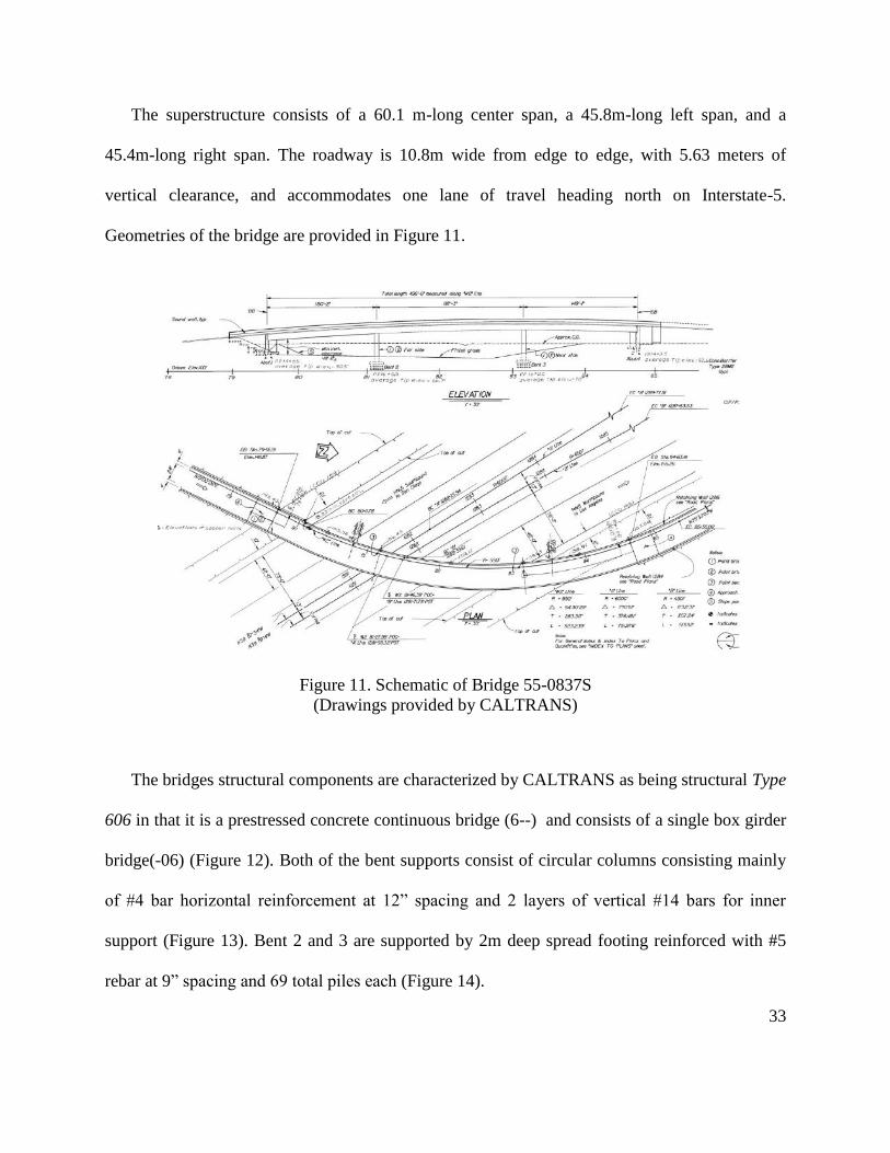
The superstructure consists of a 60.1 m-long center span, a 45.8m-long left span, and a
45.4m-long right span. The roadway is 10.8m wide from edge to edge, with 5.63 meters of
vertical clearance, and accommodates one lane of travel heading north on Interstate-5.
Geometries of the bridge are provided in Figure 11.
Figure 11. Schematic of Bridge 55-0837S
(Drawings provided by CALTRANS)
The bridges structural components are characterized by CALTRANS as being structural Type
606 in that it is a prestressed concrete continuous bridge (6--) and consists of a single box girder
bridge(-06) (Figure 12). Both of the bent supports consist of circular columns consisting mainly
of #4 bar horizontal reinforcement at 12” spacing and 2 layers of vertical #14 bars for inner
support (Figure 13). Bent 2 and 3 are supported by 2m deep spread footing reinforced with #5
rebar at 9” spacing and 69 total piles each (Figure 14).

34
Figure 12. Single box girder typical section for Bridge 55-0837S
(Drawings provided by CALTRANS)
Figure 13. Bent support cross-sections for Bridge 55-0837S
(Drawings provided by CALTRANS)

35
Figure 14. Bent support foundation typical section for Bridge 55-0837S
(Drawings provided by CALTRANS)
4.3 Linear and Nonlinear Models of Bridge 55-0837S
The finite element model of Bridge 55-0837S was originally developed using OpenSees
(Mazzoni et al. 2006) by the researchers from UCI for other research purposes. Both linear and
nonlinear models were developed from the original model for use in FR-RSA and FR-LSA
procedures in this investigation.
Due to the nature of each of the analyses performed on Bridge 55-0837S, both a linear and
nonlinear model were constructed from the original finite element model to satisfy each of the
analytical methods. In both the linear and nonlinear models, the bridge deck was modeled using
elastic beam-column elements (i.e., elasticBeamColumn in OpenSees). The nonlinear model is
identical to the linear model except that the bents were modeled using elastic beam-column

36
elements in the linear model, and as beam-column elements with distributed plasticity and linear
curvature distribution based on the non-iterative (or iterative) force formulation (i.e.,
dispBeamColumn in OpenSees) in the nonlinear model.
Consistent with the procedures described in Chapter 2, both the linear and nonlinear models
are used for different analysis purposes. The linear bridge model is used by both FR-RSA and
FR-LSA in determining the periods, mode shapes, and effective influence vectors of the bridge
through eigenvalue and static analysis respectively. The nonlinear model is used in both the FR-
RSA and FR-LSA procedures to determine the quasi-static response of the bridge. Moreover, the
nonlinear model is used in RHA which although time consuming, provides the base results used
to evaluate the accuracy of FR-RSA and FR-LSA.
4.4 Model Components
The bridge model itself is constructed using a network of nodes and their individual
properties defining a series of geometric, coordinate, and material behaviors. Element
connections are defined as being continuous across nodal points, i.e., the three translations and
three rotations (six degrees of freedom per node), and have stiffness contributions from all
elements in contact to that node (Dameron et al. 1997). The structural model is constructed by
individual property parameters defined for each of the following model components:
(1) Nodes (2) Masses (3) Materials (4) Sections (5) Elements (6) Load Patterns (7) Time
Series (8) Transformations (9) Blocks (10) Constraints

37
The finite element model allowed for individual tagging of cross sectional geometries, material
behaviors, nodal coordinates, nodal masses, element connections and other parameters for
appropriate structural representation. All structural weights were accounted for in the model for
determining the seismic response. The following sections go into detail for the bridge’s
individual components.
4.4.1 Deck System
The deck of Bridge 55-0837S was modeled using 30 elastic beam-column elements (i.e.,
elasticBeamColumn in OpenSees) as shown in Figure 15. The elastic beam-column elements are
used to model deck system to ensure it remains elastic under the applied seismic and gravity
loads. The cross-section properties determined according to CALTRANS SDC are assigned to
each of the deck elements.
Figure 15. Assignments of nodes and elements in plan view for the FE model of Bridge 55-
0837S
The elastic stiffness of the deck was defined by six principle parameters inside of the model
including: axial stiffness (EA); bending stiffness about the longitudinal and transverse axes (EIl

38
and EIt); shear stiffness about the longitudinal and transverse axes (GAl and GAt); and torsional
stiffness (GJ). A summary of the decks property for elements 1-30 is shown in Table 4.1.
Table 2. Summary of deck system properties for deck elements 1-30
Element Starting Node 1(i) i
Element End Node 1(j) j
A (m2) 7.6293
E (MPa) 276062
G (MPa) 23005.2
J (m4) 0.2099
Iz (m4) 0.2099
Iy (m4) 47.157
4.4.2 Bent Supports
Similar to the deck system, each bent was modeled using five elastic beam-column elements
(i.e., elasticBeamColumn in OpenSees) in the linear model and five inelastic beam-column
elements (i.e., dispBeamColumn in OpenSees) in the nonlinear model as shown in Figure 16. As
briefly gone over, the displacement-based beam-column elements in the nonlinear model have a
distributed-plasticity and linear curvature distribution using integration along the element based
on the Gauss-Legendre quadratic rule (Mazzoni et al. 2006).

39
Figure 16. Assignments of nodes and elements in elevation view for the FE model of Bridge 55-
0837S
Soil springs are defined at the bent bases. Consistent with the original UCI bridge model, the
rotational and translational springs were assigned stiffness values of 5.65x10¹⁰
kN-mm and 145
kN/mm respectively; however, the springs along the vertical and torsional directions are assumed
to be rigid.
4.4.3 Abutment Model Design
Previous investigations have proven the significant importance of abutment behavior, soil
structure interaction, and embankment flexibility due to their individual contributions to the total
bridge response under moderate to strong intensity ground motions. Aviram et al. (2008) proved
that embankment mobilization and the inelastic behavior of the soil material under high shear
deformation levels are able to dominate the response of the bridge and the intermediate column
bents. In order to ensure correct representation of the abutments, the systems were modeled using
linear soil-structure interaction techniques to define: (1) the stiffness of the foundation material;
(2) representations of mass and damping of the embedded and enclosed soil; and (3) equivalent
masses for the surrounding and enclosed soils (Dameron et al. 1997). The forces in the three-
dimensional spring-system are obtained from solving three equations of dynamic equilibrium,

40
corresponding to two translational motions and one rotational motion about vertical axis of the
bridge deck. Mass properties and recorded accelerations provide inertia forces for the bridge
deck while stiffness and deformation values of the bents provide their individual forces.
Springs were also assigned at the abutments to consider soil structure interaction and other
restraining effects due to presence of shear keys, wing walls, and back walls at abutments. The
following defines the vertical, transverse, and longitudinal spring definitions at abutments using
CALTRANS SDC recommendations.
Vertical Response:
Consistent with the original UCI model, the vertical component of the bridges abutment was
represented by an elastic spring with stiffness equal to 49,380 kN/mm.
Transverse Response:
According to Caltrans SDC, the stiffness along the abutment transverse direction should be
equal to 50% of the elastic transverse stiffness of the adjacent bent with consideration of the
flexibility of bent foundation. As a result, the linear elastic spring defined along the abutment
transverse direction is equal to 20.93 kN/mm.
Longitudinal Response:
Total bridge displacement in the longitudinal direction is limited by the closure of gaps if the
abutment were to be assumed infinitely stiff and strong. However since this is not the case,
consideration of additional movements at the abutments due to their flexibility and yielding is
important. Both parameters are able to significantly compromise the integrity of the entire bridge
system. In addition, movements at the abutments may be due to elastic deformation of the

41
backfill soil and slide of the entire system when supported on footings. Other source of
movements to be addressed are of that coming from inelastic deformation as a result of yielding
in the soil and flexibility of the foundation effecting force transfer due to the yielding soil. Proper
estimates of capacity/demand ratios for the different elements are calculated in order to have
suitable parameters for soil-structure interactions.
As shown in Figure 17, according to Caltrans SDC (CALTRANS 2010), the stiffness of the
equivalent elastic compression-only springs, effK , is:
/
bw bweff
eff gap bw abut
P PK
P K
where bwP is the passive pressure force resisting movement at the abutment, and where gap and
abutK are the coefficients determined from the elastic-perfectly plastic gap springs defined in the
original UCI model. As a result, effK was determined to be 28.54 kN/mm.
Figure 17. Simplification of longitudinal abutment springs
(Adapted from CALTRANS 2010)

42
CALTRANS SDC uses this bilinear idealization of the force-deformation relation to account
for longitudinal displacements being primarily restrained due to the presence of abutments. This
force-deformation relation deduces that larger longitudinal bridge displacements produce more
severe damages to abutments. As a result, a smaller stiffness should be assigned to the abutment
longitudinal springs to consider the less significant restraining action. The approximation method
provides adjustments for assessment of the abutments contribution to the overall bridges seismic
performance relative to the bent supports. These adjustments suggest varying the longitudinal
abutment spring stiffness from 0.1 to 1.0 effK , which can be further determined from an iterative
process based on the longitudinal displacement of the bridge. To validate the FR-RSA and FR-
LSA procedures for varying abutment contributions to overall systems response, three stiffness
values of 0.10 effK , 0.55 effK , and 1.00 effK were considered for the investigation.
4.4.6 Zero-Length Members
To ensure the structural integrity and the composite behavior between the bridge deck and
bent supports, zero-length members were used to model the connection between joints. In order
to capture the structural response and associated damage to bridge connections, modeling of the
localized inelastic deformation occurring at the member end regions were identified by shaded
areas in Figure 18 (b). Consistent with the OpenSees Command Manual (Mazzoni et al. 2006),
these member end deformations consist of two components: (1) the flexural deformation that
causes inelastic strains in the longitudinal bars and concrete, and (2) the member end rotation,
due to reinforcement slip. This reinforcement slip is the result of strain penetration along a
portion of the fully anchored bars into the adjoining concrete members, e.g., deck-to-bent and

43
bent-to-footing connections for Bridge 55-0837S (Figure 18 (a)), during the elastic and inelastic
response of the structure.
(a) (b)
Figure 18. Actual bent support cross-section (a) and expected inelastic regions at bent support (b)
(Adapted from CALTRANS 2010)
To account for these model strain penetration effects (or fixed end rotations), zero-length
section members were used. Zero-length elements were placed at intersections between the
flexural member and an adjoining member representing a footing or joint and serve as
connection two points at the same coordinate, as demonstrated in Figure 19. A list of zero-length
elements used in the finite element model is demonstrated in Table 3.

44
Table 3. Finite Element Model Zero-length member summary
Location Member # Starting Node End Node
Abutment #1 41 411 41
42 421 42
Abutment #2 43 431 43
44 441 44
Bent #2 201 211 21
Bent #3 301 311 31
The zero-length members allow for a duplicate node (with the same coordinates) to be
between a fiber-based beam-column element and the adjoining concrete element. Since the
translational degrees-of-freedom from these new nodes are constrained to existing nodes, sliding
of the beam-column elements under lateral loads is prevented, due to shear resistance not being
included in the zero-length members.
Figure 19. Location of zero-length member to a beam-column element
(Adapted from CALTRANS 2010)

45
The zero-length members are modeled in OpenSees as having a unit length such that the
element deformations (i.e., elongation and rotation) are equal to the section deformations (i.e.,
axial strain and curvature). The nodes from the zero-length member join the two nodes at a
connection by multiple UniaxialMaterial objects to represent the force-deformation relation for
the element.
4.5 Consideration of Bridge Orientations
To validate the simplified procedures under a wider range of the parameters, it was
determined to rotate the bridge orientation to achieve different bridge-to-fault angles and. As
shown in Figure 20 (b), the initial orientation of the bridge is assumed to be the one with the
chord connecting the two abutments perpendicular to the fault line direction. Moreover, it was
assumed at the initial bridge orientation that the two bents are equally spaced on each side of the
fault as shown in Figure 20 (b). The angle from the initial orientation to the orientation of
interest, , is used to define different bridge orientations from the fault rupture line as
demonstrated in Figure 20 (a). In this investigation, the clockwise and counterclockwise angles
are respectively assigned “+” and “-“ signs. Rotating the bridge about its left abutment, one can
determine that the angle, varies between -38 degrees and 53 degrees as shown in Figure 21. It
was determined to select the bridge along the following orientation angles: - 53, 45, 30, 21, 15,
0, -15, -30, and -38 degrees, for further investigation.

46
Figure 20. Definition of bridge orientation angle
Figure 21. Bridge orientation limit definitions
z
x
L1 L1
Z(z)
X (x)
FAULT LINE
0° ORIENTATION
Z
X
FAULT LINE
DEFINITION OF ORIENTATION ANGLE
Z
X
FAULT LINE
53° ORIENTATION :
UPPER ROTATION LIMIT
z
x
53°
Z
X
FAULT LINE
-38° ORIENTATION :
LOWER ROTATION LIMIT
z
x
38°

47
CHAPTER 5: RESULTS AND DISCUSSION
5.1 Response Quantities of Interest
The response quantities of interest include the displacement demands at the abutments and
bents (see Abutments 1 and 4, and Bents 2 and 3 in Figure 10). The maximum absolute values
of the abutment longitudinal and transverse displacement components were output for
comparison purpose. Abutment displacements in longitudinal and transverse directions were
obtained from the transformation of the displacements along global Z and X axes as
demonstrated in the following equation:
cos sin
sin cos
z Z
x X
where angle represents the angle between global and local axes.
In FR-RSA, the abutment longitudinal and transverse displacement components associated
with each mode were combined using CQC as described in Section 2.2.2. Moreover, as required
in CALTRANS SDC (CALTRANS 2010), the bent rigid body movements caused by foundation
deformations were taken into account when calculating the bent displacement demands. The
maximum resultant bent displacements were obtained from the square root of the maximum
absolute values of the two horizontal bent displacement components and compared in this
investigation.

48
5.2 Results
As discussed in Chapter 4, two parameters, the stiffness of the longitudinal abutment springs
(selected to be 0.10 effK , 0.55 effK , and 1.00 effK ) and the bridge orientation angle ( 53, 45,
30, 21, 15, 0, -15,-30 and -38 degrees), were varied in the investigation to evaluate the robustness
and adequacy of FR-RSA and FR-LSA under the practical ranges of the parameters. Results
from the FR-RSA and FR-LSA procedures are differentiated into two categories: ground motions
(GM) and design spectrum (DS), which respectively represent the results obtained from:
(1) FR-RSA with pseudo-accelerations for a selected mode computed from elastic RHA of
equivalent SDF analysis motion pairs (GM)
(2) FR-RSA with pseudo-acceleration for a selected mode computed from the idealized
CALTRANS SDC design spectrum (DS)
(3) FR-LSA with peak ground accelerations selected from each ground motion (GM)
(4) FR-LSA with 2.5 eff gom u maximum spectral acceleration from CALTRANS elastic
design spectrum (DS)
Moreover, for the results from the GM category, the average values of the bridge responses from
the 10 ground motions pairs are presented.
As consistent observations can be obtained from all considered cases, Figures 22 through 24
only present results from 0 for all three 0.10 effK , 0.55 effK , 1.00 effK stiffness cases. A
complete set of results for all orientations stiffness cases can be found in Appendix C.

49
Figure 22. Results for = 0 degrees and longitudinal abutment stiffness = 0.10Keff
Figure 23. Results for = 0 degrees and longitudinal abutment stiffness = 0.55Keff

50
Figure 24. Results for = 0 degrees and longitudinal abutment stiffness = 1.00Keff
5.3 Discussion of Results
As presented in Figures 22 through 24 for the 0 degree orientation, results consistently
show that the FR-RSA and FR-LSA procedures provide reasonable estimates for the seismic
demands of the bridge. Discrepancies in results range from 0.29 m maximum to 0.01 m
minimum for all three 0.10 effK , 0.55 effK , and 1.00 effK stiffness cases. The following sections
go into discussion of the results for both abutment and bent support values as well as the
accuracy of the procedures in estimating these values:
5.3.1 Abutments
For all cases, abutment longitudinal displacements began slightly smaller than transverse
displacements for orientations closer to 0 and then proportionally grew larger for
orientations moving away from the start position. This was expected since the more skewed the

51
bridge-to-fault orientations became from its original perpendicular position, the more effect the
fault-rupture would have on the bridges longitudinal components, even after being combined
through CQC. This is demonstrated in Appendix C (Figures C.2- C.4 and Figure C.34-C.36)
where the bridge displays higher longitudinal displacements at its rotation limits of = 53 and
= -38. However, regardless of orientation definition or stiffness case, deformations at abutments
from RHA were able to be reasonably estimated using FR-RSA and FR-LSA procedures.
Accuracy of both procedures for both transverse and longitudinal directions at abutments is
presented in Figures 25-28 for all orientation cases.
Figure 25. Accuracy of FR-RSA for abutments in transverse direction at all orientations using
both GM and DS for longitudinal abutment stiffness = 1.00Keff

52
Figure 26. Accuracy of FR-RSA for abutments in longitudinal directions at all orientations using
both GM and DS for longitudinal abutment stiffness = 1.00Keff
Figure 27. Accuracy of FR-LSA for abutments in transverse directions at all orientations using
both GM and DS for longitudinal abutment stiffness = 1.00Keff

53
Figure 28. Accuracy of FR-LSA for abutments in longitudinal directions at all orientations using
both GM and DS for longitudinal abutment stiffness = 1.00Keff
5.3.2 Bent Supports
Deformations provided for bent supports were found to be just as accurately approximated
using the two procedures as to abutment deformations. In many cases such as for = -15, 0, 15
degrees results at both Bent #2 and Bent #3 were found to be considerably accurate, almost
identical, to values received from the “exact” RHA procedure. A couple cases displayed slightly
conservative deformations for Bent #2 and slightly underestimated deformations for Bent #3, as
well as vice versa, within the same orientation set. Divergence in values may be attributed to the
fault-rupture being located between bent supports and actual influence of the rupture fluctuating
between being mostly applied to Bent #2 or Bent #3 while moving through rotations. As
previously mentioned, the influence of the fault to each bent support is simulated and accounted
for through the idealization of spatially-varying excitations as a proportional multiple-support
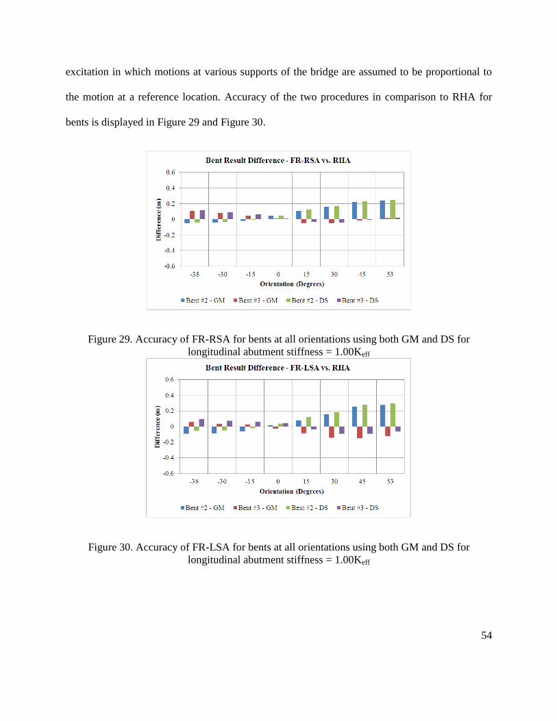
54
excitation in which motions at various supports of the bridge are assumed to be proportional to
the motion at a reference location. Accuracy of the two procedures in comparison to RHA for
bents is displayed in Figure 29 and Figure 30.
Figure 29. Accuracy of FR-RSA for bents at all orientations using both GM and DS for
longitudinal abutment stiffness = 1.00Keff
Figure 30. Accuracy of FR-LSA for bents at all orientations using both GM and DS for
longitudinal abutment stiffness = 1.00Keff

55
5.4.3 Accuracy of Procedures
The accuracy of the total (quasi-static plus dynamic) demands for the three-span curved
bridge were evaluated for both FR-RSA and FR-LSA proposed approximation procedures. As
seen in the results, the proposed FR-RSA procedure is able to consistently show reasonable
estimates for the seismic demands of the bridge. As described in Chapter 2, the FR-RSA
procedure presented is the most general method of analysis and holds no computational
peculiarities related to earthquake engineering analysis (Camata et al. 2007). For all orientations
and three stiffness cases, FR-RSA was able to produce deformations within 0.01 to 0.25 m from
the “exact” RHA procedure. These relatively small discrepancies could be attributed to the
approximation of using modal participation factors n , and the computation of the “effective”
influence vector eff to distinguish all of the bridges significant modes in dynamic analysis. Even
with this divergence, there are several cases where FR-RSA generated essentially identical
results to the more rigorous RHA procedure.
Similar to FR-RSA, FR-LSA provided reasonably accurate deformation results at both abutment
and bent support levels, however doing so while avoiding dynamic analysis. As seen in the
Figures 25 through 28, deformations resulted slightly more conservative than the FR-RSA and
RHA procedures primarily due to the use of the conservative estimate of response spectral
accelerations. This was the same conclusion as in the study provided by Goel and Chopra (Goel
and Chopra 2008a, 2008b, 2009a, 2009b) for ordinary straight bridges. As described in Chapter 2
for FR-LSA procedure, the value of A was conservatively approximated to be 5 times gou , i.e.
2.5 goA u , thus making the peak dynamic response be computed from the application of lateral

56
forces equal to 2.5 eff gom u applied on the structure. Slightly even simpler than FR-RSA, FR-LSA
avoids computation of the vibrational periods of the bridge and the rise-time of the fault-offset.
However it must also be noted that there are a couple cases where FR-LSA underestimates the
structures seismic response at both abutment and bents such as demonstrated in Figure C.35 for
in Appendix C.

57
CHAPTER 6: CONCLUSIONS &
RECOMMENDATIONS
The presented investigation for analysis of the three-span curved Bridge 55-0837S crossing
fault-rupture zones has been implemented through four principal phases: (1) appraisal and
analysis of the proposed approximation procedures (FR-RSA and FR-LSA) crossing fault-
rupture zones in extension to a three-span curved bridge; (2) evaluation of proper ground motion
selection and application; (3) modeling of the three-span curved bridge (Bridge 55-0837S); and
(4) accuracy of results from procedures in comparison to the “exact” but much more rigorous
RHA procedure. Following is the summary of conclusions and recommendations from this
investigation:
One of the principal assumptions in the development of both FR-RSA and FR-LSA
procedures was the computation of a total peak value of the bridges seismic response
through superposition of peak values from the quasi-static and dynamic parts of the
response. As defined in Chapter 2, the peak quasi-static response in both methods is
computed by static analysis of the bridge under all ground displacement offsets
associated with fault rupture applied simultaneously. In FR-RSA and FR-LSA, the peak
dynamic responses are respectively estimated from combination of the peak modal
responses using the complete-quadratic-combination rule and the linear static analysis of
the bridge under appropriate equivalent seismic forces respectively. Both approximation
procedures have great advantages in practicality and application for bridge engineers,
such as FR-RSA using the response spectrum directly to account for all significant modes
in dynamic analysis, and FR-LSA avoiding computation of the structures vibrational

58
periods and estimation of rise time of fault offset through a much simpler static analysis
of the bridge under appropriate applied loads. Both procedures were found to provide
reasonably accurate results for all definitions and stiffness cases, deeming them valid
and practical for use in design and analysis of three-span curved bridges.
The presented procedures use the idealization of spatially-varying excitations as a
proportional multiple-support excitation in which motions at various supports of the
bridge are assumed to be proportional to the motion at a reference location. Identical to
the conclusion construed for the study provided by Goel and Chopra (2008a), this
idealization is judged as being valid for spatially-varying ground motions in close
proximity to faults under the varying definitions.
The finite element nonlinear model of Bridge 55-0837S was able to effectively capture
the behavior of the bridge accounting for the Design Fault Offset. While being identical
to the linear model, the nonlinear model included plastic hinges and beam-column
elements with distributed plasticity and linear curvature distribution based on the non-
iterative force formulation (i.e., dispBeamColumn in OpenSees). Both FR-RSA and FR-
LSA procedures computed their quasi-static response using the nonlinear model by
applying gravity loads and foundation offsets due to the fault-rupture. The foundation
offset was simulated by applying support displacements with values equal to FP FP
l gou and
FN FN
l gou at support l in fault-parallel and fault-normal directions, respectively.

59
The abutment longitudinal and transverse displacement components associated with each
mode were combined using the complete quadratic completion (CQC) rule. Using current
CALTRANS SDC (CALTRANS 2010) recommendations for maximum bent
displacement demands accounting for bent rigid body movements caused by foundation
deformations, a total deformation result was accurately able to be provided through the
combination procedure. Moreover, the resultant maximum bent displacements obtained
from the square root of the maximum absolute values of the two horizontal bent
displacement components were also able to represent the structures final deformation
response.
The fault-rupture “effective” influence vectors at all structural degrees of freedom eff
used in the procedures was able to properly account for simultaneous static application of
all support displacements approximated as FP FP
l gou and FN FN
l gou at support l in fault-
parallel and fault-normal directions, respectively. The dynamic response FP
QSr and FP
QSr , of
the bridge due to fault-parallel and fault-normal ground motions can be conservatively
estimated by the static analysis of the linear structure due to the lateral forced equal to
max
FP FP
effm A in the fault-parallel direction, and max
FN FN
effm A in the fault-normal direction.
While in specific cases, the approximation of the peak values of the spectral acceleration
for ground hazards ( maxA ) resulted in slightly conservative values for the bridges seismic
response, overall it was still able to provide reasonably accurate responses for the bridges
displacements.

60
By taking the mean of the 10 geometric means, for all ground motion sets, CALTRANS
proposed a smooth target design spectrum to represent the group of 10 record sets (Figure
9). The proposed design spectrum would allow for approximate yet valid representation
of the entire set of ground motions while shortening the analysis time to a single run per
analysis instead of 10 to include each set. The CALTRANS design spectrum (DS) was
indeed able to consistently provide an accurate representation of all the ground motions
(GM). This stayed true for both abutments and bents for all orientations and stiffness
cases, making use of the design spectrum not only valid but efficient. Differences (if any)
between results from using GM and DS are seen as negligible for application purposes.
To ensure the structural integrity and the composite behavior between the bridge deck
and bent supports, zero-length members were used to model the connection between
joints. Member end deformations consisted of two components: (1) the flexural
deformation that causes inelastic strains in the longitudinal bars and concrete, and (2) the
member end rotation, due to reinforcement slip. The nodes from the zero-length members
joined two nodes at a connection by multiple UniaxialMaterial objects and effectively
represented and recorded the force-deformation relation for the bridges elements.
Conclusions from the studies performed by Goel and Chopra (2008a, 2008b, 2009a, 2009b)
on idealistic three- and four-span straight bridges perpendicular to faults determined the two
principal analysis methods investigated in this paper. The current investigation furthermore
proved validity of these procedures to estimate peak seismic responses on a slightly more

61
complex three-span curved bridge accurate enough for practical design purposes. Though
logistically demanding for bridge engineers, nonlinear response history analysis (RHA) of
bridges in this investigation is seen and compared to as being the “exact” solution to the
structures dynamic response and is many times needed for bridges on “lifeline” routes, however
this procedure may be too onerous for “ordinary” bridges which form a majority of today’s
infrastructure.
It must be noted that even though the FR-RSA procedure was able to provide valid estimates
for the bridge’s seismic response, FR-LSA did not require full computation of the bridge’s
vibration periods or mode effects as compared to the other methods. By simply performing a
linear static analysis of the bridge due to appropriate lateral forces, FR-LSA indirectly considers
contributions from all vibration modes, ground offset across the fault, and the shape of the
response spectrum due to its close proximity to the fault-ruptured zone. Due to the point of the
investigation being to find the most simple analysis method while providing accurate results, FR-
LSA is recommended for further extension onto more complex bridge designs.

62
CHAPTER 7: RECOMMENDATIONS FOR
SUBSEQUENT STUDY
While the analysis completed in Year 1 of this project provides better insight on applicability
and validity of FR-RSA and FR-LSA in seismic analysis and design of the curved bridges
crossing earthquake faults, it is recognized that the bridge example considered in the analysis
contains only three spans, for which the bridge displacement caused by the earthquake fault
offset is relatively simple due to the absence of interaction of multiple bents on the same side of
the fault. To further promote the use of FR-RSA and FR-LSA in practice, it is necessary to
evaluate their adequacy in the context of other bridge examples in the future. A possible next
focus of work could include analysis of a four-span bridge (Bridge 55-0939G) crossing fault, in
which special considerations are given to the fault locations or to a skewed bridge where the
effect of the actual fault rupture could alter due to the abutment location.
Subsequent studies could also expand on using nonlinear spring models provided by UC
Irvine to represent actual soil-structure interaction systems defining a gap at abutments to serve
as a limit of deformation due to unseating or striking effects from excitations. While the
transverse spring system used in this investigation is consistent with CALTRANS SDC
recommendations, no clear guidelines are provided for modeling of shear keys, effects of
separation, impact, and slippage of soil-abutment interfaces. Such effects exhibit highly
nonlinear behaviors and could be addressed with more detail in following studies.

63
REFERENCES
1. Afshin, K., & Amjadian, M. (2010). An Approximate Method for Dynamic Analysis of
Highway Bridges with Continuous Rigid Deck. Engineering Structures, 32(9), 2850-
2860.
2. Aviram, A., MAckie, K. R., & Stojadinovic, B. (2008). Effect of Abutment Modeling on
the Seismic Response of Bridge Structures. Earthquake Engineering & Structural
Dynamics, 7(4), 395-402.
3. CALTRANS. (2010). Seismic Design Criteria.
4. Camata, G., Sarnia, A., & Spacone, E. (2007). Seismic Risk Assesment of a Existing
Reinforced Concrete Bridge. Pescara, Italy.
5. Chen, Y. (2001). Nonlinear Seismic Analysis of Bridges: Pracitical Approach and
Comperative Study.
6. City-Data. (2010). Retrieved from http://www.city-data.com/bridges/bridges-Anaheim-
California4.html
7. Dameron, R. A., Sobash, V. P., & Lam, I. P. (1997). Nonlinear Seismic Analysis of
Bridge Structures: Foundation-Soil Representation and Ground Motion Input. Computers
& Structures, 64(5-6), 1251-1269.
8. Dreger, H. G., Chopra, A. K., & Larson, S. (2007). Near-Fault Seismic Ground Motions:
Earthquake Engineering Research Center.
9. Filippou, F. C. (1992). Nonlinear Static and Dynamic Analysis of Reinforced Concrete
Subassemblages.
10. Ghasemi, H. (2004). Bolu Viaduct: Damage Assessment and Retrofit Strategy: FHWA.
11. Ghusn, G. E., & Saiidi, M. (1986). Simple Histeretic Element for Biaxial Bending of R/C
Colulumns (Nonlinear Earthquake Analysis of Bridge Systems). Nevada University,
Reno.
12. Goel, R. K., & Chopra, A. K. (2008a). Analysis of Ordinary Bridges Crossing Fault-
Rupture Zones. University of California, Berkeley, CA: Earthquake Engineering
Research Center.

64
13. Goel, R. K., & Chopra, A. K. (2008b). Role of Shear Keys in Seismic Behaior of Bridges
Crossing Fault-Rupture Zones. Journal of Bridge Engineering, 13(4), 398-408.
14. Goel, R. K., & Chopra, A. K. (2009a). Linear Analysis of Ordinary Bridges Crossing
Fault-Rupture Zones. Journal of Bridge Engineering, 13(4), 398-408.
15. Goel, R. K., & Chopra, A. K. (2009b). Nonlinear Analysis of Ordinary Bridges Crossing
Fault-Rupture Zones. Journal of Bridge Engineering, 14(3), 216-224.
16. Hanks, T. C., & Bakun, W. H. (2002). A Bilinear Source-Scaling Model for M-log A
Observations of Continental Earthquakes. Seismological American Society(92), 1841-
1846.
17. Honegger, D., Nyman, D., & Johnson, E. (2004). Trans-Alaska Pipeline System
Performance in 2002 Denali Fault. Earthquake Spectra, 20(3), 707-738.
18. Imbsen, R. A., & Penzien, J. (1986). Evaluation of Energy-Absorption Characteristics of
Highway Bridges under Seismic Conditions (Vol. 1): University of California, Berkeley.
19. Ingham, T. J., Rodriguez, S., & Nader, M. (1997). Nonlinear Analysis of the Vincent
Thomas Bridge for Seismic Retrofit. Computers & Structures, 64(5-6), 1221-1238.
20. Kawashima, K., Takahashi, Y., & Ge, H. (2008). Damage of Bridges in 2008 Wenchuan,
China Earthquake. Tokyo, Japan: Tokyo Institute of Technology.
21. Mazzoni, S., Scott, M. H., & Fenves, G. L. e. a. (2006). OpenSees Command Language
Manual.
22. Nyman, D. J., Johnson, E. R., & Roach, C. H. (2006). Trans-Alask Pipeline Emergency
Response and Recovery. Paper presented at the Sixth U.S. Conference on Lifeline
Earthquake Engineering, Long Beach, CA.
23. Shantz, T., & Chiou, B. (2010). Creation of Record Set for Use in Fault Crossing Study:
California Department of Transportation.
24. Toki, K. (1980). Nonlinear Response of Continuous Bridge Subjected to Traveling
Seismic Wave. Paper presented at the 7th World Conference of Earthquake Engineering,
Istanbul, Turkey.
25. Tseng, W.S., & Penzien, J. (1975). Seismic Analysis of Long Multiple-Span Highway
Bridges. Earthquake Engineering & Structural Dynamics, 4(1), 3-24.

65
26. Wang, J., Carr, A. J., Cooke, N., & Moss, P. J. (2009). Response of a 344 m long bridge
to non-uniform earthquake ground motions. Engineering Structures.
27. Wells, D. L., & Coppersmith, J. J. (1994). New Empirical Relationships Among
Magnitude, Rupture Length, Width, Rupture Area, and Surface Displacement.
Seismological American Society(84), 974-1002.
28. Zanardo, G., Hao, H., & Modena, C. (2002). Seismic Response of Multi-Span Simply
Supported Bridges to a Varying Earthquake Ground Motion. Earthquake Engineering &
Structural Dynamics, 31(6), 1325-1345.

66
APPENDICES

67
Appendix A : Ground Motion Summary

68
The following section provides both time histories and pseudo-acceleration responses for
Bridge-Normal (BN) and Bridge-Parallel (BP) components, left and right of fault. The following
table summarizes the ground motion record sets provided by CALTRANS and used in this
investigation.
Table Summary of considered base ground motion pairs*
Set No. Component 1 Component 2 Time step (sec) Number of Points
1 LOMAP-BVC220 LOMAP-BVC310 0.005 5918
2 LOMAP-HSP000 LOMAP-HSP090 0.005 11990
3 LOMAP-HDA165 LOMAP-HDA255 0.005 7928
4 KOBE-FUK000 KOBE-FUK090 0.02 3900
5 NORTHR-SAR000 NORTHR-SAR270 0.01 3600
6 NORTHR-NEE090 NORTHR-NEE180 0.01 4800
7 KOBE-OSA000 KOBE-OSA090 0.02 6000
8 KOBE-ABN000 KOBE-ABN090 0.01 14000
9 ITALY-A-TDG000 ITALY-A-TDG270 0.0029 18216
10 SFERN-WND143 SFERN-WND233 0.001 7997 *selected from the NGA database.

69
Figure A.1 - Time series summary for Record Set 1 in Bridge-Normal direction
Figure A.2 - Pseudo-Acceleration Response Summary for Record Set 1in Bridge-Normal
direction

70
Figure A.3 - Time series summary for Record Set 1 in Bridge-Parallel direction
Figure A.4 - Pseudo-Acceleration Response Summary for Record Set 1in Bridge-Normal
direction

71
Figure A.5 - Time series summary for Record Set 2 in Bridge-Normal direction
Figure A.6 - Pseudo-Acceleration Response Summary for Record Set 2 in Bridge-Normal
direction

72
Figure A.7 - Time series summary for Record Set 2 in Bridge-Parallel direction
Figure A.8 - Pseudo-Acceleration Response Summary for Record Set 2 in Bridge-Parallel
direction
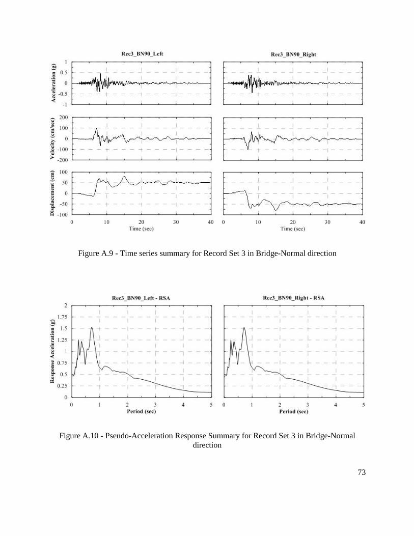
73
Figure A.9 - Time series summary for Record Set 3 in Bridge-Normal direction
Figure A.10 - Pseudo-Acceleration Response Summary for Record Set 3 in Bridge-Normal
direction

74
Figure A.11 - Time series summary for Record Set 3 in Bridge-Parallel direction
Figure A.12 - Pseudo-Acceleration Response Summary for Record Set 3 in Bridge-Parallel
direction

75
Figure A.13 - Time series summary for Record Set 4 in Bridge-Normal direction
Figure A.14 - Pseudo-Acceleration Response Summary for Record Set 4 in Bridge-Normal
direction

76
Figure A.15 - Time series summary for Record Set 4 in Bridge-Parallel direction
Figure A.16 - Pseudo-Acceleration Response Summary for Record Set 4 in Bridge-Parallel
direction

77
Figure A.17 - Time series summary for Record Set 5 in Bridge-Normal direction
Figure A.18 - Pseudo-Acceleration Response Summary for Record Set 5 in Bridge-Normal
direction

78
Figure A.19 - Time series summary for Record Set 5 in Bridge-Parallel direction
Figure A.20 - Pseudo-Acceleration Response Summary for Record Set 5 in Bridge-Parallel
direction

79
Figure A.21 - Time series summary for Record Set 6 in Bridge-Normal direction
Figure A.22 - Pseudo-Acceleration Response Summary for Record Set 6 in Bridge-Normal
direction

80
Figure A.23 - Time series summary for Record Set 6 in Bridge-Parallel direction
Figure A.24 - Pseudo-Acceleration Response Summary for Record Set 6 in Bridge-Parallel
direction

81
Figure A.25 - Time series summary for Record Set 7 in Bridge-Normal direction
Figure A.26 - Pseudo-Acceleration Response Summary for Record Set 7 in Bridge-Normal
direction

82
Figure A.27 - Time series summary for Record Set 7 in Bridge-Parallel direction
Figure A.28 - Pseudo-Acceleration Response Summary for Record Set 7 in Bridge-Parallel
direction

83
Figure A.29 - Time series summary for Record Set 8 in Bridge-Normal direction
Figure A.30 - Pseudo-Acceleration Response Summary for Record Set 8 in Bridge-Normal
direction

84
Figure A.31 - Time series summary for Record Set 8 in Bridge-Parallel direction
Figure A.32 - Pseudo-Acceleration Response Summary for Record Set 8 in Bridge-Parallel
direction

85
Figure A.33 - Time series summary for Record Set 9 in Bridge-Normal direction
Figure A.34 - Pseudo-Acceleration Response Summary for Record Set 9 in Bridge-Normal
direction

86
Figure A.35 - Time series summary for Record Set 9 in Bridge-Parallel direction
Figure A.36 - Pseudo-Acceleration Response Summary for Record Set 9 in Bridge-Parallel
direction

87
Figure A.37 - Time series summary for Record Set 10 in Bridge-Normal direction
Figure A.38 - Pseudo-Acceleration Response Summary for Record Set 10 in Bridge-Normal
direction

88
Figure A.39 - Time series summary for Record Set 10 in Bridge-Parallel direction
Figure A.40 - Pseudo-Acceleration Response Summary for Record Set 10 in Bridge-Parallel
direction

89
Appendix B : Mode Shapes and Periods

90
Z
X
FAULT LINE
z
x
38°
Figure B.1 Sketch of Bridge 55-0837S
when .
Figure B.2 - Mode Shapes and Period summary for
(Longitudinal Abutment Stiffness= 0.10Keff)

91
Figure B.3 - Mode Shapes and Period summary for
(Longitudinal Abutment Stiffness= 0.55Keff)
Figure B.4 - Mode Shapes and Period summary for
(Longitudinal Abutment Stiffness= 1.00Keff)

92
FAULT LINE
z
x
Z
X
30°
Figure B.5 - Sketch of Bridge 55-
0837S when .
Figure B.6 - Mode Shapes and Period summary for
(Longitudinal Abutment Stiffness= 0.10Keff)
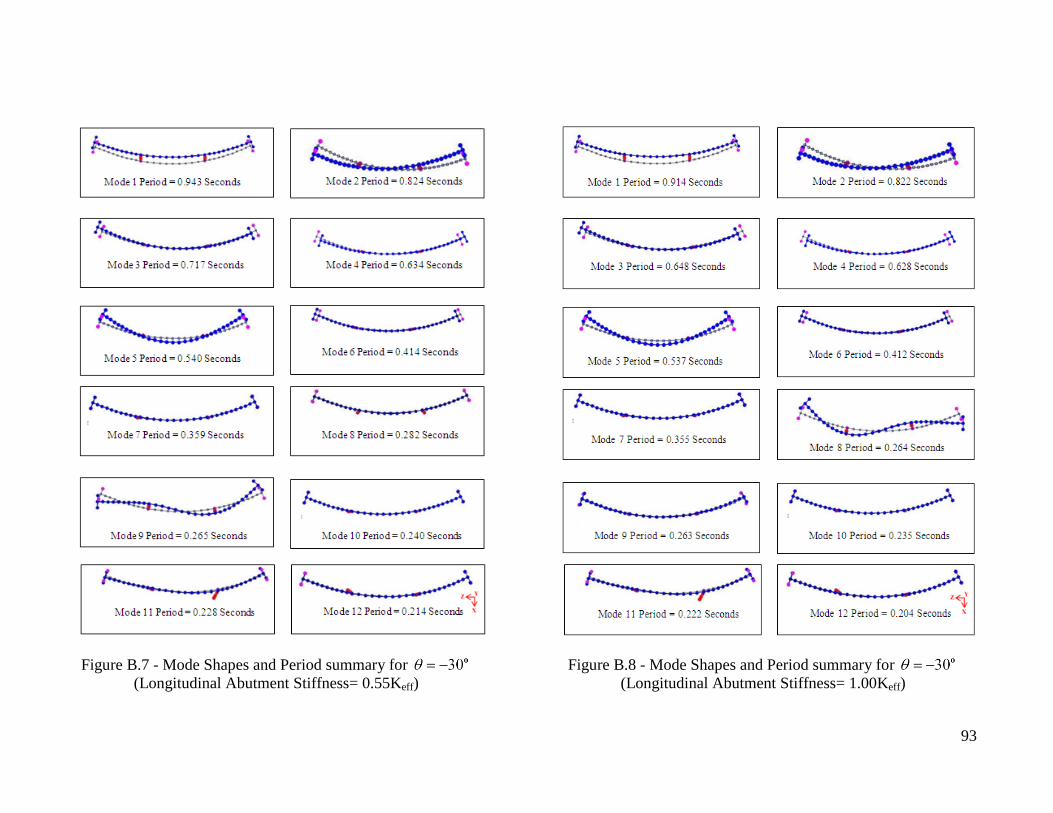
93
Figure B.7 - Mode Shapes and Period summary for
(Longitudinal Abutment Stiffness= 0.55Keff)
Figure B.8 - Mode Shapes and Period summary for
(Longitudinal Abutment Stiffness= 1.00Keff)

94
Z
X
FAULT LINE
z
x
15°
Figure B.9 - Sketch of Bridge 55-0837S when
.
Figure B.10 - Mode Shapes and Period summary for
(Longitudinal Abutment Stiffness= 0.10Keff)

95
Figure B.11 - Mode Shapes and Period summary for
(Longitudinal Abutment Stiffness= 0.55Keff)
Figure B.12 - Mode Shapes and Period summary for
(Longitudinal Abutment Stiffness= 1.00Keff)

96
Z(z)
X (x)
FAULT LINE
Figure B.13- Sketch of Bridge 55-0837S when
Figure B.14 - Mode Shapes and Period summary for
(Longitudinal Abutment Stiffness= 0.10Keff)

97
Figure B.15 - Mode Shapes and Period summary for
(Longitudinal Abutment Stiffness= 0.55Keff)
Figure B.16 - Mode Shapes and Period summary for
(Longitudinal Abutment Stiffness= 1.00Keff)

98
Z
X
FAULT LINE
15°
z
x
Figure B.17 - Sketch of Bridge 55-0837S when
Figure B.18 - Mode Shapes and Period summary for
(Longitudinal Abutment Stiffness= 0.10Keff)

99
Figure B.19 - Mode Shapes and Period summary for
(Longitudinal Abutment Stiffness= 0.55Keff)
Figure B.20 - Mode Shapes and Period summary for
(Longitudinal Abutment Stiffness= 1.00Keff)

100
z
x
Z
X
FAULT LINE
21°
Figure B.21 - Sketch of Bridge 55-0837S when
Figure B.22 - Mode Shapes and Period summary for
(Longitudinal Abutment Stiffness= 0.10Keff)

101
Figure B.23 - Mode Shapes and Period summary for
(Longitudinal Abutment Stiffness= 0.55Keff)
Figure B.24 - Mode Shapes and Period summary for
(Longitudinal Abutment Stiffness= 1.00Keff)

102
z
x
Z
X
FAULT LINE
30°
Figure B.25 - Sketch of Bridge 55-0837S when
Figure B.26 - Mode Shapes and Period summary for
(Longitudinal Abutment Stiffness= 0.10Keff)

103
Figure B.27 Mode Shapes and Period summary for
(Longitudinal Abutment Stiffness= 0.55Keff)
Figure B.28 - Mode Shapes and Period summary for
(Longitudinal Abutment Stiffness= 1.00Keff)

104
Z
X
FAULT LINE
45°
z
x
Figure B.29 - Sketch of Bridge 55-0837S when
Figure B.30 - Mode Shapes and Period summary for
(Longitudinal Abutment Stiffness= 0.10Keff)

105
Figure B.31 - Mode Shapes and Period summary for
(Longitudinal Abutment Stiffness= 0.55Keff)
Figure B.32 - Mode Shapes and Period summary for
(Longitudinal Abutment Stiffness= 1.00Keff)

106
Z
X
FAULT LINE
z
x
53°
Figure B.34 - Mode Shapes and Period summary for
(Longitudinal Abutment Stiffness= 0.10Keff)
Figure B.33 - Sketch of Bridge 55-0837S
when

107
Figure B.35 - Mode Shapes and Period summary for
(Longitudinal Abutment Stiffness= 0.55Keff)
Figure B.36 - Mode Shapes and Period summary for
(Longitudinal Abutment Stiffness= 1.00Keff)

108
Appendix C : Complete Result Comparisons of Bridge 55-0837S

109
Figure C.1 - Sketch of Bridge 55-0837S when 38 o
Figure C.2 - Results of Bridge 55-0837S when 38 o and
longitudinal abutment stiffness = 0.10 effK .
Z
X
FAULT LINE
z
x
38°

110
Figure C.3 - Results of Bridge 55-0837S when 38 o and
longitudinal abutment stiffness = 0.55 effK
Figure C.4 - Results of Bridge 55-0837S when 38 o and
longitudinal abutment stiffness =1.00 effK .

111
Figure C.5 - Sketch of Bridge 55-0837S when 30 o
Figure C.6 - Results of Bridge 55-0837S when 30 o and
longitudinal abutment stiffness = 0.10 effK
FAULT LINE
z
x
Z
X
30°

112
Figure C.7 - Results of Bridge 55-0837S when 30 o and
longitudinal abutment stiffness = 0.55 effK
Figure C.8 - Results of Bridge 55-0837S when 30 o and
longitudinal abutment stiffness =1.00 effK
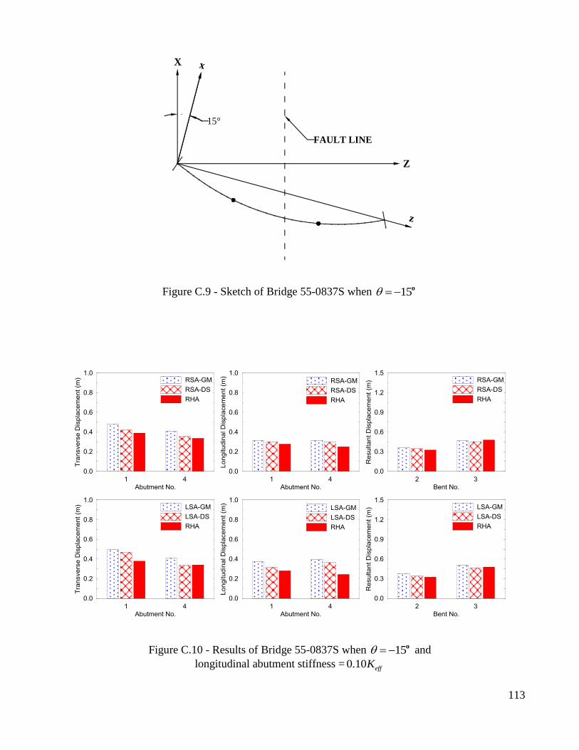
113
Figure C.9 - Sketch of Bridge 55-0837S when 15 o
Figure C.10 - Results of Bridge 55-0837S when 15 o and
longitudinal abutment stiffness = 0.10 effK
Z
X
FAULT LINE
z
x
15°

114
Figure C.11 - Results of Bridge 55-0837S when 15 o and
longitudinal abutment stiffness = 0.55 effK
Figure C.12 - Results of Bridge 55-0837S when 15 o and
longitudinal abutment stiffness =1.00 effK

115
Figure C.13 - Sketch of Bridge 55-0837S when 0 o
Figure C.14 - Results of Bridge 55-0837S when 0 o and
longitudinal abutment stiffness = 0.10 effK
Z(z)
X (x)
FAULT LINE

116
Figure C.15 - Results of Bridge 55-0837S when 0 o and
longitudinal abutment stiffness = 0.55 effK
Figure C.16 - Results of Bridge 55-0837S when 0 o and
longitudinal abutment stiffness =1.00 effK

117
Figure C.17 - Sketch of Bridge 55-0837S when 15 o
Figure C.18 - Results of Bridge 55-0837S when 15 o and
longitudinal abutment stiffness = 0.10 effK
Z
X
FAULT LINE
15°
z
x

118
Figure C.19 - Results of Bridge 55-0837S when 15 o and
longitudinal abutment stiffness = 0.55 effK
Figure C.20 - Results of Bridge 55-0837S when 15 o and
longitudinal abutment stiffness =1.00 effK

119
Figure C.21 - Sketch of Bridge 55-0837S when 21 o
Figure C.22 - Results of Bridge 55-0837S when 21 o and
longitudinal abutment stiffness = 0.10 effK .
z
x
Z
X
FAULT LINE
21°

120
Figure C.23 - Results of Bridge 55-0837S when 21 o and
longitudinal abutment stiffness = 0.55 effK
Figure C.24 - Results of Bridge 55-0837S when 21 o and
longitudinal abutment stiffness =1.00 effK

121
Figure C.25 - Sketch of Bridge 55-0837S when 30 o
Figure C.26 - Results of Bridge 55-0837S when 30 o and
longitudinal abutment stiffness = 0.10 effK
z
x
Z
X
FAULT LINE
30°

122
Figure C.27 - Results of Bridge 55-0837S when 30 o and
longitudinal abutment stiffness = 0.55 effK
Figure C.28 - Results of Bridge 55-0837S when 30 o and
longitudinal abutment stiffness =1.00 effK

123
Figure C.29 - Sketch of Bridge 55-0837S when 45 o
Figure C.30 - Results of Bridge 55-0837S when 30 o and
longitudinal abutment stiffness = 0.10 effK
Z
X
FAULT LINE
45°
z
x

124
Figure C.31 - Results of Bridge 55-0837S when 45 o and
longitudinal abutment stiffness = 0.55 effK
Figure C.32 - Results of Bridge 55-0837S when 45 o and
longitudinal abutment stiffness =1.00 effK
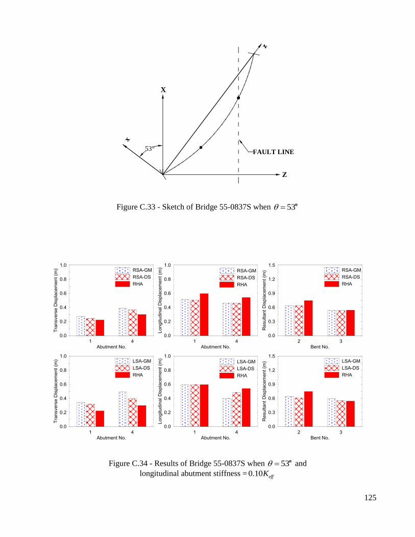
125
Figure C.33 - Sketch of Bridge 55-0837S when 53 o
Figure C.34 - Results of Bridge 55-0837S when 53 o and
longitudinal abutment stiffness = 0.10 effK
Z
X
FAULT LINE
z
x
53°

126
Figure C.35 - Results of Bridge 55-0837S when 53 o and
longitudinal abutment stiffness = 0.55 effK
Figure C.36 - Results of Bridge 55-0837S when 53 o and
longitudinal abutment stiffness =1.00 effK