Brian Reich (NC State) M. Fuentes (VCU), J. Warren (Yale ...

Spatial risk estimation of adverse pregnancy outcomes due to pollution

Brian Reich (NC State)

M. Fuentes (VCU), J. Warren (Yale), A. Herring (UNC), P. Langlois (Texas SHE)

TIES 2016

Scientific Motivation: Why Preterm Birth?

• Preterm birth (delivery before 37 completed weeks of gestation) amajor cause of infant morbidity and mortality

• Cause of roughly 50% of preterm births unknown

• Institute of Medicine (IOM) estimates average first-year medical costsare 10 times greater for a preterm relative to a term birth

• IOM estimates total cost over $26 billion annually (over $50K perpreterm birth) including hospital costs, special education, etc.

• US national incidence around 12%; around 1.6 times higher inAfrican-American than in white and/or Hispanic women

References: March of Dimes Prematurity Campaign (2010); Martin etal. (2010).

NC State University 2 / 45TIES 2016

Brian Reich

Scientific Motivation: Preterm birth and air pollution

Specific Results of Literature Review linking preterm birth and airpollution:

• Preterm Birth: Current studies about the impact of air pollution onpreterm birth are not conclusive, but indicate a potential associationand the need for further research.

• More information is needed to examine:• Effect of different pollutants• Most vulnerable periods of the pregnancy

• Significant pollutants include particulate matter.

References: Sram et al. (2005) and the U.S. EPA PM and CO IntegratedScientific Assessments (2009 and 2010).


Brian Reich

Risk Factors for Preterm Birth

• Black mothers at higher risk (16-18%)

• Low socioeconomic and educational status

• Low and high maternal ages

• Single marital status

• Working long hours

• Frequent hard physical labor

• Mechanisms by which maternal demographics are related to pretermbirth are still unknown

• Source: Romero (2008)


Brian Reich

Statistical Motivation: Challenges

• Incorporate spatial analysis of environmental health data, typically notconsidered in classical birth outcome epidemiological studies

• Develop new statistical methodology to allow the ability to uncovertrue relationships between ambient air pollution exposure and pretermbirth

• Create statistical models to identify the specific critical windowsduring the pregnancy when high exposures to pollutants morenegatively affect the birth outcomes

• Characterize the uncertainty in models and data in the risk assessment


Brian Reich

Data Sources and Information

Texas Vital Records Data:

• Data provided by the Birth Defects Epidemiology andSurveillance Branch of the Texas Department of State HealthServices in collaboration with Dr. Peter Langlois

• Full birth records from all births in Texas where

1 Mother resided at delivery in a region and time period covered by thebirth defect registry

• 1997-2004

2 demographic information


Brian Reich


Figure: Birth Weight (grams) and Gest. Age (weeks) Histograms

Variable Mean SD Min Max N

Birth Weight (grams) 3286.73 579.79 0.00 8098.00 2625678

Gest. Age (weeks) 38.59 2.17 12.00 48.00 2588704

Table: Summary Statistics for Texas Vital Records Data, 1997-2004


Brian Reich


Infant/Fetus and Pregnancy Information Included:

• Case/Control Status

• Sex

• Birth Weight

• Pregnancy Outcome

• Plurality of Pregnancy

• Gestational Age Estimates

• Number of Previous Live Births

Mother/Father Information Included:

• Age

• Birthplace

• Race/Ethnicity

• Education


Brian Reich


Geocoding Information:

• Each birth is geocoded to the residence at delivery

• Included Information:

• Latitude/Longitude• City, County• Street Address, ZIP Code• Geocoding Accuracy

• Texas (1995-2002) study found that 68% of pregnant women didnot move between date of conception and date of birth (Nuckolset al. (2004))

• Of the women who did move, 49% stayed very close geographically(same water supply source)


Brian Reich


Figure: Birth Locations in Texas, 1997-2004


Brian Reich


Pollution Data Sources:

• Fused Air and Deposition Surfaces Data (FSD): 2001-2006• EPA product which calibrates Community Multiscale Air Quality

(CMAQ) data using observed monitoring data• Nation-wide daily data available on the CMAQ grids (12km x 12km

and 36km x 36km spatial resolution)• Ozone- Maximum daily 8-hour average (parts per billion (ppb))• PM2.5- Daily average (micrograms per cubic meter (ug/m3))

• Air Quality System (AQS) Data (monitoring data): 2000-2004• Ozone- Maximum daily 8-hour average (parts per million (ppm))• PM2.5- Daily average (micrograms per cubic meter (ug/m3))

Weather Data (2000-2004): Daily temperature, dew point, cloudcover,and windspeed.


Brian Reich

FSD Model

• Y (s): Monitoring data for site s

• Q(Aj): CMAQ numerical model output for grid cell Aj

• Z (s): True pollution value for site s

• Latent process, unobservable without measurement error

Model:

• Y (s) = Z (s) + ε(s)

• ε(s)iid∼ N(0, σ2

ε ); measurement error

• Q(s) = a(s) + b(s)Z (s) + γ(s)

• a(s): Additive bias associated with CMAQ data• b(s): Multiplicative bias associated with the CMAQ data

• γ(s)iid∼ N(0, σ2

γ); random error


Brian Reich

FSD Model

• Q(Aj) =∫Aja(s)ds + b

∫AjZ (s)ds +

∫Ajγ(s)ds

• CMAQ data given as areal estimates

• Z (s) = µ(s) + ν(s)• µ(s): Large scale spatial trend• ν: Gaussian process with specified spatial covariance structure• b(s) constant over space based on recommendations by EPA

• Values simulated from posterior predictive distribution (ppd) forspatial prediction

• ppd: P(Z (s ′)|Y,Q)

• EPA adopted this model (Fuentes and Raftery (2005)) and extendedit to space-time to create their FSD product (McMillan et al. (2010))


Brian Reich


Pollution Data Sources (Texas Only):

• Air Quality System (AQS) Data: 2000-2004• Ozone- Maximum daily 8-hour average (parts per million (ppm))• PM2.5- Daily average (micrograms per cubic meter (ug/m3))

Weather Data: 2000-2004

• Daily weather data from the National Climatic Center (NCDC)


Brian Reich

Active Texas Pollution Monitors: 2000-2004

Figure: Ozone Monitor Locations (Red), PM2.5 Monitor Locations (Blue)


Brian Reich

Previous Work

• Exposure to pollution during pregnancy typically handled throughtrimester, monthly, and pregnancy averages; fit separately usingmultiple models for different exposure windows, including separatemodels for different pollutants (Xu et al. (1995); Bobak (2000); Linet al. (2001))

• Method is inefficient and does not allow us to jointly identify specificperiods across the entire pregnancy in a continuous manner

• Empirical analysis indicated that increased exposure to PM2.5 andozone during the pregnancy lead to statistically significant decreasesin gestational age and birth weight


Brian Reich

Empirical Analysis

• Jointly modeled birth weight and gestational age in Harris County(includes Houston), 2002-2003

• Fit a mixture of bivariate normal distributions with independentcomponents

• Used first trimester averages of PM2.5 and ozone as the pollutionexposure (models fit separately)

• Modeled the mean using mother/father covariate information


Brian Reich

Empirical Analysis Results

• Found that a mixture of two bivariate normal distributions providedthe best (based on AIC/BIC) fit for the data

• Distribution 1: About 8% of the population was from this distribution• This group of births had much lower birth weights and gestational ages

on average than a typical birth

• Distribution 2: About 92% of the population was from thisdistribution

• This group of births had typical birth weights and gestational ages onaverage


Brian Reich


Groups Identified by Mixture Model Analysis

25 30 35 40 45

010

0020

0030

0040

0050

0060

00

Gest. Age (Weeks)

Wei

ght (

Gra

ms)

Figure: Identified Births from Distribution 1 (Red) and Distribution 2 (Black)


Brian Reich

Distribution 1, Birth Weight Results (grams)

Variable Estimate (PM2.5 Model) p-value

Intercept 2611.81 <0.0001

Female vs. Male Baby -73.28 0.0484

Mother ≥ 40 vs. Mother 10 − 19 -558.44 0.0015

Black vs. White Mother (Non-Hispanic) -547.25 <0.0001

First Trimester Pollution Average -162.46 <0.0001

Table: PM2.5 Model Results.

Variable Estimate (Ozone Model) p-value

Intercept 2659.17 <0.0001

Female vs. Male Baby -86.81 0.0185

Mother ≥ 40 vs. Mother 10 − 19 -548.23 0.0012



Table: Ozone Model Results.NC State University 20 / 45

TIES 2016Brian Reich

Distribution 1, Gest. Age Results (weeks)

Variable Estimate (PM2.5 Model) p-value

Intercept 35.79 <0.0001

Mother ≥ 40 vs. Mother 10 − 19 -2.58 0.0035



Table: PM2.5 Model Results.

Variable Estimate (Ozone Model) p-value

Intercept 35.99 <0.0001

Mother ≥ 40 vs. Mother 10 − 19 -2.61 <0.0001

Black vs. White Mother (Non-Hispanic) -2.47 0.0023


Table: Ozone Model Results.


Brian Reich


• High number of observations in distribution 2 caused most effects tobe found significant

• Pollution exposure effects were found to be significantly negative

• An increased exposure to PM2.5 and ozone in the first trimesterappears to be associated with a decrease in birth weight andgestational age for both distributions


Brian Reich

Preterm Birth Model: Trimester Average Approach

Yi |β,θind∼ Bern(pi (β,θ)),

pi (β,θ) = probability birth i results in preterm birth,

logit(pi (β,θ)) = xiTβ +

2∑j=1

2∑k=1

θ(j , k)Zj(ti (k), s(i)),

• k : Trimester of the pregnancy• Zj(ti (k), s(i)): Trimester average of pollutant j at location s(i)

according to calendar date range ti (k)• Pollution exposures based on woman specific dates of pregnancy and

calculated using observations from the nearest pollution monitor• Similar to models used by Bobak (2000), Ritz et al. (2007), and Liu

et al. (2003)


Brian Reich

Preterm Birth Model: Trimester Average Approach

θ(j , k): Effect of the concentration of air pollutant j on trimester k on theprobability of PTB for woman i

• Model often fit in the Frequentist setting with the θ parametersconsidered as fixed, ignoring the correlation that exists between thetrimester averages and across pollutants (Ritz et al. (2000); Ritz etal. (2007); Xu et al. (1995))

• Changes in the pollution effects across space most often times ignored

• To avoid this multicollinearity, multiple models are usually fit:

• One pollutant at a time• One pollution exposure measure at at time


Brian Reich

New Methodology

• Incorporating the spatial aspect into the modeling procedure to allowthe pollution exposure effects to change over the geographic domainof interest

• Allowing a more continuous form of exposure over the entirepregnancy by introducing weekly exposures

• Allowing multiple pollutants to be modeled simultaneously whileaccounting for the correlation between the effects

• Bayesian framework allows for flexible solution to correctlycharacterize the uncertainty associated with the parameter estimates


Brian Reich

General Framework

Weather Model:

W(s, t) = µ(s, t) + e1(s, t) + ε1(s, t)

• W(s, t): Vector of weather observations at various locations andtimes

• µ(s, t): Large scale spatial and temporal trend of the data

• e1(s, t): Spatially and temporally correlated zero mean Gaussianprocess

• ε1(s, t)iid∼ N(0, σ2

1)

• Measurement error associated with the weather monitors


Brian Reich

General Framework

Pollution Model:

• Zj(s, t): AQS monitor observation for pollutant j at location sand time t

Zj(s, t) = Zj(s, t) + ε2(s, t)

• Zj(s, t): True pollution process for pollutant j at location s andtime t

• Unobservable without measurement error

• ε2(s, t)iid∼ N(0, σ2

2)

• Measurement error associated with the pollution monitors


Brian Reich

General Framework

True Pollution Process:

Zj(s, t) = W(s, t)Tδ + e2(s, t)

• e2(s, t): Spatially and temporally correlated zero mean Gaussianprocess

• Posterior distribution of the weather covariates used as prior inthis stage (Gelman 2004)

• “Directional” Bayesian approach provides computational benefit as wellas not allowing the final health stage of modeling to provideinformation about the initial weather stage

• Values of Zj(s, t) simulated from the ppd, P(Zj |Zj), at eachwoman’s location during the relevant pregnancy window


Brian Reich

New Methodology

Preterm Birth Model:

Yi |β,θind∼ Bern(pi(β,θ)),

pi(β,θ) = probability birth i results in preterm birth,

Φ−1(pi(β,θ)) = xiTβ +

2∑j=1

min(gai ,36)∑w=1

θ(j ,w , si)Zj(ti(w), si),

• Φ−1(.): Inverse cumulative distribution function of the standardnormal distribution

• ‘gai ’ is the gestational age (weeks) for birth i


Brian Reich

Modeling the Pollution Coefficients

• θ(j ,w , s): Pollutant specific spatially and temporally varyingcoefficients

• Represent the effects of the concentration of air pollutant j at locations on pregnancy week w on the probability of PTB for woman i

• Zj(ti (w), si ) represents the pollution exposure for pollutant j oncalendar week ti (w) at location si

• Ozone and PM2.5 used in the analysis


Brian Reich

New Methodology

Prior Process of θ Parameters:

θ ∼ MVN(0,φ0Σ), with entries of φ0Σ are given by,

cov(θ(j ,w , s), θ(j′,w

′, s

′))

= φ0 exp{−φ1||s − s

′ || − φ2|w − w′ | − φ3I (j 6= j

′)}

• Exponential covariance structure provides relatively simpleparameterization which allows separate degrees of shrinkage across airpollutants j , pregnancy week w , and location s

• Allows us to overcome multicollinearity introduced by using weeklyexposures

• Computationally feasible because Σ is the Kronecker product of 3smaller dimension correlation matrices


Brian Reich

Application

Harris County, Texas 2002-2004. Mother’s first birth. Single births.Birth defect births included (live births only).

Harris County, TX:• Third largest county in the US as of July, 2009

• 4,070,989 estimated people in the county during this time• Los Angeles County, CA and Cook County, IL only larger counties

• Includes Houston, TX which is provides a large amount ofheterogeneity to our study population

• Excellent pollution and weather monitor coverage in the county


Brian Reich

Harris County Pollution Monitors: 2002-2004

Figure: Harris County, TX (Left); Active Harris County and Surrounding AreaOzone (Red) and PM2.5 (Blue) Pollution Monitors, 2002-2004 (Right)


Brian Reich

Significant Parental Covariate Results

Percentiles

Covariate Mean 0.025 0.50 0.975

Maternal Race

Black vs. White 0.1498 0.0187 0.1495 0.2827

Paternal Race

Other vs. White -0.1887 –0.3369 –0.1886 –0.0410

Maternal Age Group

20− 24 vs. 10− 19 –0.0742 –0.1382 –0.0742 –0.0103

35− 39 vs. 10− 19 0.1108 0.0093 0.1108 0.2114

≥ 40 vs. 10− 19 0.2959 0.1176 0.2968 0.4701

Female vs. Male Baby –0.0675 –0.1080 –0.0677 –0.0265

Table: Significant covariate results for the predicted AQS data, 2002-2004. The MC error for the means ranged from 0.0001to 0.0007 with an average value of 0.0004.


Brian Reich

Model Comparisons

• Fit a simplified version of the model to compare results with thenewly introduced model

• Simplified model represents a basic multiple regression model whichignores the correlation that exists between the pollution coefficients

• Does not have the ability to identify the windows of critical exposurethroughout the pregnancy for either pollutant

• Fit trimester average model

• Both models fit in the Bayesian setting


Brian Reich

Trimester Average and Basic Multiple Regression ModelGraphical Results

0.0 0.5 1.0 1.5 2.0 2.5 3.0

−0.

020.

000.

020.

040.

060.

080.

100.

12

PM2.5

Trimester

Effe

ct

0.0 0.5 1.0 1.5 2.0 2.5 3.0

−0.

020.

000.

020.

040.

060.

080.

100.

12

Ozone

Trimester

Effe

ct

0 5 10 15 20 25 30 35

−0.

050.

000.

05

PM2.5

Week

Effe

ct

0 5 10 15 20 25 30 35

−0.

10−

0.05

0.00

0.05

Ozone

Week

Effe

ct

Figure: Susceptible windows of exposure for the trimester average and basic multiple regression

models using predicted AQS Data, Harris County, Texas, 2002-2004. Posterior means and 95%

credible intervals are displayed.


Brian Reich

Graphical Results of Exposure Windows

0 5 10 15 20 25 30 35

−0.

020.

000.

020.

04

PM2.5

Week

Effe

ct

0 5 10 15 20 25 30 35

−0.

02−

0.01

0.00

0.01

0.02

0.03

Ozone

Week

Effe

ct

Figure: Susceptible windows of exposure using predicted AQS Data, Harris County, Texas,2002-2004. Posterior means and 95% credible intervals are displayed.


Brian Reich

Model Comparison Results

Model pD DIC

Newly Introduced 41.84 17226.00Trimester Average 26.01 17268.06

Basic Multiple Regression 93.96 17267.03

Table: DIC results. pD is the effective number of parameters for the given model.

Differences of more than 10 in DIC rule out the model with a higher value (Lunn etal. 2000).


Brian Reich

Sensitivity Analysis Results

Model pD DIC

2 Uniforms 41.84 17226.001 Gamma, 1 Uniform 41.87 17226.10

2 Gammas 41.96 17226.50

Table: DIC results. pD is the effective number of parameters for the given model.

The table summarizes the fit of the newly introduced model using different combinationsof prior distributions for the covariance hyper-parameters.


Brian Reich

Extension to Space

Each County Fit Separately: Uniforms for Covariance Parameter Priors

0 5 10 15 20 25 30 35

−0.

04−

0.02

0.00

0.02

0.04

0.06

0.08

PM2.5

Week

Effe

ct

0 5 10 15 20 25 30 35

−0.

050.

000.

05

Ozone

Week

Effe

ct

0 5 10 15 20 25 30 35

−0.

04−

0.02

0.00

0.02

0.04

0.06

0.08

PM2.5

Week

Effe

ct

0 5 10 15 20 25 30 35

−0.

050.

000.

05

Ozone

Week

Effe

ct

0 5 10 15 20 25 30 35

−0.

04−

0.02

0.00

0.02

0.04

0.06

0.08

PM2.5

Week

Effe

ct

0 5 10 15 20 25 30 35

−0.

050.

000.

05

Ozone

Week

Effe

ct

Figure: Dallas County (left), Travis County (center), and Harris County (right) critical windowsof exposure.


Brian Reich

Extension to Space

Each County Fit Separately: Uniforms for Covariance Parameter Priors

0 5 10 15 20 25 30 35

−0.

04−

0.02

0.00

0.02

0.04

0.06

0.08

PM2.5

Week

Effe

ct

0 5 10 15 20 25 30 35

−0.

050.

000.

05

Ozone

Week

Effe

ct

0 5 10 15 20 25 30 35

−0.

04−

0.02

0.00

0.02

0.04

0.06

0.08

PM2.5

Week

Effe

ct

0 5 10 15 20 25 30 35

−0.

050.

000.

05

Ozone

Week

Effe

ct

0 5 10 15 20 25 30 35

−0.

04−

0.02

0.00

0.02

0.04

0.06

0.08

PM2.5

Week

Effe

ct

0 5 10 15 20 25 30 35

−0.

050.

000.

05

Ozone

Week

Effe

ct



Brian Reich

Results across Space

Fully Spatial Model: Uniforms for Covariance Parameter Priors

0 5 10 15 20 25 30 35

−0.

04−

0.02

0.00

0.02

0.04

0.06

0.08

PM2.5

Week

Effe

ct

0 5 10 15 20 25 30 35

−0.

050.

000.

05

Ozone

Week

Effe

ct

0 5 10 15 20 25 30 35

−0.

04−

0.02

0.00

0.02

0.04

0.06

0.08

PM2.5

Week

Effe

ct

0 5 10 15 20 25 30 35

−0.

050.

000.

05

Ozone

Week

Effe

ct

0 5 10 15 20 25 30 35

−0.

04−

0.02

0.00

0.02

0.04

0.06

0.08

PM2.5

Week

Effe

ct

0 5 10 15 20 25 30 35

−0.

050.

000.

05

Ozone

Week

Effe

ct



Brian Reich

Biological Justification

• Exposure to air pollution early in the first trimester may interfere withthe delivery of oxygen and nutrients to the fetus

• Exposure may affect the placental development during the earlystages of pregnancy

• Exposure may trigger inflammation, leading to PTB

• Exact explanation for how pollution affects the fetus not yet identified

• Some studies show that ultra fine particles can enter the mother’slungs and penetrate the lung barriers, entering the bloodstream

• Particles can then travel to the organs, such as the brain andplacenta, and may cause problems for the fetus

References: Ritz and Wilhelm (2008).


Brian Reich

Conclusions

• More accurately identified periods during pregnancy where increasedexposure to pollution leads to increased probability of preterm birth

• Multiple pollutants handled jointly

• Increased evidence linking harmful air pollution and birth outcomeswhile extending the results for preterm births

• More information uncovered and made available to the pregnantpopulation which could potentially decrease the rate of preterm birthand lead to healthier birth outcomes in general


Brian Reich

Part II

Spatial variable selection

Brian Reich

Department of StatisticsNorth Carolina State University

July 21, 2016

Joint work with Jian Kang and Ana-Maria Staicu

Brian Reich Spatial variable selection

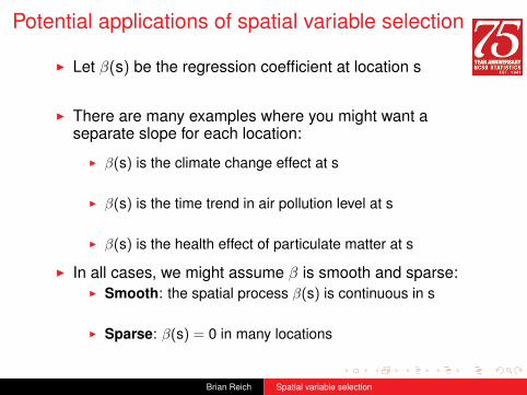
Potential applications of spatial variable selection

I Let β(s) be the regression coefficient at location s

I There are many examples where you might want aseparate slope for each location:

I β(s) is the climate change effect at s

I β(s) is the time trend in air pollution level at s

I β(s) is the health effect of particulate matter at s

I In all cases, we might assume β is smooth and sparse:I Smooth: the spatial process β(s) is continuous in s

I Sparse: β(s) = 0 in many locations


Example 1: Time trends in tropospheric ozone

I The EPA uses a monitoring network to regulate ozone

I Our objective is to identify areas with changing ozone

I We perform a linear regression at each site and study thetime-trend estimates

I The next slide has the first-stage estimates (z-scores)


Example 1: Time trends in tropospheric ozone

−90 −85 −80 −75 −70

2530

3540

45

Longitude

Latit

ude

−4

−2

0

2


Example 2: Health effects of PM

I Fine particulate matter (PM) has been linked with severaladverse health outcomes and is regulated by the EPA

I Literature has shown a spatially-varying effect

I This may be due to variation in PM composition orsusceptibility of the population

I We analyze data for 22 chemical species of PM (elementalcarbon, nitrates, etc)

I The objective is to identify which species are most harmful,and to study spatial variation in the effects


Example 2: Health effects of PM

I Let Yit be the number of Medicare CVD hospitaladmissions on day t in county i

I We analyze the 117 largest US counties and have datafrom 2000-2008

I Our model is

log[E(Yit )] = confounders +

p=22∑j=1

Xitjβj(si)

where Xitj is the value of pollutant j and βj(si) is its effect

I We want to find j and s for which βj(s) 6= 0


Effect of elemental carbon

−1.0

−0.5

0.0

0.5

1.0


Example 3: EEG study of alcoholism

I Goal: Study the relationship between the brain activity asmeasured through EEG signals and genetic predispositionto alcoholism

I Data: 77 alcoholic subjects + 45 controls

I 64 electrodes sampled at 128Hz

I We use spatial variable selection to identify regions mostpredictive of alcoholism


Scaler-on-image regression framework

I Observed data for i th subject

I Yi is scalar outcome

I Xi = (Xi1, ...,Xip)T is an image/array

Model: Yi =∑p

j=1 β(sj)Xij + εi

I β is the coefficient image

I Assumption: β is a sparse and piecewise smooth function

I εiiid∼ N(0, σ2)

I Goal: Estimation and inference of β(s)


Literature on scaler-on-image regression

I Frequentist approaches: Tibshirani (JRSSB1996);Tibshirani et al. (JRSSB05), Tibshirani & Taylor (AoS11);Reiss & Ogden (Bcs10); Wang & Zhu (Bka15)

I No inferential methods available using this approach

I Bayesian approaches: Goldsmith et al. (JCGS14); Li et al.(AoAS15)

I Stability issues due to using two latent processes to modelthe coefficient image

I No smooth transition between the zero areas and non-zeroparts


Soft Thresholded Gaussian Process (ST GP)I Bayesian approach: assume β(s) = gc{Z (s)}

I Z (s) is latent Gaussian Process with zero mean andcontinuous covariance function

I gc is real-valued function with gc(z) = sign(z)(|z| − c) forsome specified threshold c

−4 −2 0 2 4

−3

−2

−1

01

23

z

g_c(

z)


Low-rank spatial model representation

Higdon et al (1999):

Z (s) = Kh(s− τ1)a1 + . . .+ Kh(s− τL)aL

I Kh is local kernel function with Kernel bandwidth h(e.g. tapered Gaussian kernels with bandwidth h)

I The τl ’s are fixed spatial knots

I Dimension is reduced from p to L, which makes it possibleto handle large images


CAR model

I Use conditionally autoregressive (CAR) prior to account forlarge-scale spatial dependence in the al (Nychka, et alJCGS15)

I The CAR prior can be defined by the full conditionaldistribution of one site given all others:

al |ak for all k 6= l ∼ N(ρal , σ2a/ml),

I al is the mean of a at site l ’s ml neighbors

I ρ ∈ (0,1) controls the strength of spatial dependence

I σ2a controls the variance


Illustration - Kernel smoothing (a→ Z )

al

t1

t 2

−2

−1

0

1

2

Zj

s1

s 2

−2

−1

0

1

2


Illustration - Soft thresholding (Z → β)

Zj

s1

s 2

−2

−1

0

1

2

βj

s1

s 2

−0.5

0.0

0.5


Illustration - Sparsity

βj

s1

s 2

−0.5

0.0

0.5

I(βj ≠ 0)

s1

s 2

0.0

0.2

0.4

0.6

0.8

1.0


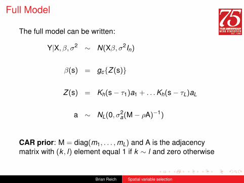
Full Model

The full model can be written:

Y|X, β, σ2 ∼ N(Xβ, σ2In)

β(s) = gc{Z (s)}

Z (s) = Kh(s− τ1)a1 + . . .Kh(s− τL)aL

a ∼ NL(0, σ2a(M− ρA)−1)

CAR prior: M = diag(m1, . . . ,mL) and A is the adjacencymatrix with (k , l) element equal 1 if k ∼ l and zero otherwise


Advantages/novelties

I The proposed method uses a single spatial process tocontrol both sparsity and smoothness

I As a result there is a gradual transition between zero andnon-zero regions

I Allows full inference and stable computations

I It allows us to study theoretical properties

I Easily extended to incorporate additional covariates orgeneralized responses


Theoretical properties

Proof of large support: Assume the true signal β0(s) is (i)piecewise smooth, (ii) sparse, and (iii) continuous. If thereexists a latent process Z (s) such that β0(s) = gc{Z (s)}. Thenthe STGP β(s) satisfies

Π(‖β(s)− β0(s)‖∞ < ε

)> 0 for all ε > 0

Posterior consistency: Assume regularity conditions for thedesign matrix of Xi ’s, and of kernel K and that true signal β0 isas above. The number of spatial locations p is such thatlog(p) = o(n). Then as n→∞, the posterior distributionsatisfies

Π[‖β(s)− β0(s)‖∞ < ε | Y,X

]→ 1


Simulation study set-upI Model: Yi ∼ Normal

(∑pj=1 β(sj)Xij , σ

2)

I Images are generated on a 30×30 grid so p = 900

I True signal β(s) is either:

5 10 15 20 25 30

510

1520

2530

Five peaks

0.0

0.1

0.2

0.3

0.4

5 10 15 20 25 305

1015

2025

30

Triangle

0.00

0.05

0.10

0.15

0.20


Set-up (cont’d)

The covariates are generated at the p locations using either anexponential correlation or to share structure (“SS”) with βA1. Xi ∼ GP(0,Exp(ρX )); ‘Exp(3)’ or ’Exp(6)’

A2. Xi(s) = eiβ(sj) + 0.5Ui(s)

ei ∼ N(0, τ2) , Ui ∼ GP(0,Exp(3)); ‘SS (2)’ or ‘SS(4)’

5 10 15 20 25 30

510

1520

2530

s1

s2

−2

−1

0

1

2

5 10 15 20 25 30

510

1520

2530

s1

s2

−2

−1

0

1

2

5 10 15 20 25 30

510

1520

2530

s1

s2

−2

−1

0

1


Performance evaluation

I Assess performance using MSE and computing time

I We compare ST GP with:

I Lasso (Tibshirani, JRSSB1996)

I Fused lasso (Tibshirani et al JRSSB05, Tibshirani & TaylorAoS11)

I fPCR: smoothing the image Xi first (Xiao et al JRSSB13)and then doing functional principal component regression

I Ising: Bayesian Scalar on Image regression (Goldsmith etal JCGS14)

I GP: the non-threshold GP prior


Results: MSE (× 1,000)

Sample size n = 100, standard deviation of conditionalresponse σ = 5. Results based on 100 simulations.

True β Cov(X) Fused lasso fPCR Ising GP ST GP5 peaks Exp(3) 18.48 3.67 4.44 2.63 1.65

Exp(6) 2.66 3.33 4.14 2.07 1.93Triangle Exp(3) 18.08 1.83 2.75 1.80 0.82

Exp(6) 4.32 1.63 2.64 1.76 0.88SS(2) 70.65 0.98 2.77 3.28 1.40SS(4) 71.23 0.34 3.18 3.39 1.81


Results: Time (minutes) when n = 100

True β Cov (X ) Fused lasso fPCR Ising GP ST GP5 peaks Exp(3) 16.77 5.40 27.61 4.81 17.69


Recall EEG dataI Yi = 1 for alcoholics and Yi = 0 otherwise

I Xi is a 60×128 image

20 40 60 80 100 120

1020

3040

5060

Mean − Alcoholics

Time

Nod

e

−6

−4

−2

0

2

4

6

20 40 60 80 100 12010

2030

4050

60

Mean − Non−alcoholics

Time

Nod

e

−6

−4

−2

0

2

4

6

I Goal: Study EEG correlates of genetic predisposition toalcoholism


Implementation details

I Probit regression: Prob(Yi = 1|Xi , β) = Φ[∑

j Xijβ(sj)]

I We use knots in every other column and row, with adifferent CAR dependence parameter in each direction

I The prior for the threshold c is somewhat informative,

c ∼ Uniform(1.43,1.96)

I This gives about 5-15% inclusion probability


Estimated β(s)

20 40 60 80 100 120

1020

3040

5060

Lasso

Ele

ctro

de

−0.05

−0.04

−0.03

−0.02

−0.01

0.00

20 40 60 80 100 120

1020

3040

5060

fPCA

−0.02

−0.01

0.00

0.01

0.02


Estimated β(s)

20 40 60 80 100 120

1020

3040

5060

GP

Time

Ele

ctro

de

−0.06

−0.04

−0.02

0.00

0.02

0.04

20 40 60 80 100 120

1020

3040

5060

STGP

Time

−0.030

−0.025

−0.020

−0.015

−0.010

−0.005

0.000


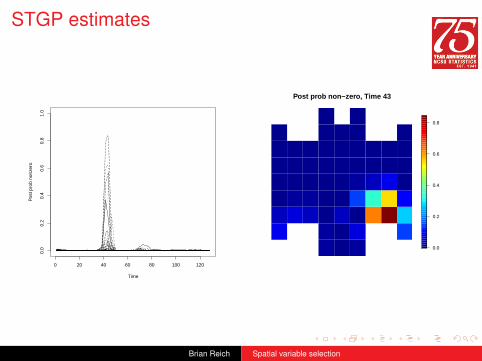
STGP estimates

0 20 40 60 80 100 120

0.0

0.2

0.4

0.6

0.8

1.0

Time

Pos

t pro

b no

nzer

o

Post prob non−zero, Time 43

0.0

0.2

0.4

0.6

0.8


STGP estimates

Posterior mean, Time 43

−0.04

−0.03

−0.02

−0.01

0.00

0.01

Posterior mean, Time 44

−0.04

−0.03

−0.02

−0.01

0.00

0.01


ROC from 5-fold CV

Specificity

Sen

sitiv

ity

0.0

0.2

0.4

0.6

0.8

1.0

1.0 0.8 0.6 0.4 0.2 0.0

Lasso (AUC = 0.77)fPCA (AUC = 0.797)GP (AUC = 0.788)STGP (AUC = 0.833)


Recall: Health effects of PM

I Let Yit be the number of Medicare CVD hospitaladmissions on day t in county i

I We analyze the 117 largest US counties and have datafrom 2000-2008

I Our model is

log[E(Yit )] = confounders +

p=22∑j=1

Xitjβj(si)

where Xitj is the value of pollutant j and βj(si) is its effect.

I We want to find j and s for which βj(s) 6= 0


Posterior mean effect by site and pollutant

−1.0

−0.5

0.0

0.5

1.0

NE Mid Atl S Atl ESC WSC ENC WNC Mtn Pac

SulfNitrSili

El COr CSodi

AmmoAlumArse

BromCalcChloChroCopp

IronLeadMagn

NickPotaTita

VanaZinc


Posterior mean EC effects

−1.0

−0.5

0.0

0.5

1.0


Posterior EC effects grouped by region

●●●●●●

●●●●●●●●●●●●●●●●●● ●

●●●●●●●●

●●●●

●●●●●●●●●

●

●●●●

●●●

●●●●●

●

●

●●

●●●

●

●●●●●●

●●●●●●

●●●●

●●●●●

●●●●●●●●●●●

●●

●

●●●●●●

●

●●●●●●

−1

01

23

β ●●●●●● ●●●●

●●●●

●●●●●●●●●● ●

●●●●●●●●●

●●●●●●●●

●●●

●●

●●●●

●●●

●●●●●●

●●●

●●●

●

●●●●●●

●●●●●●

●●●●

●●●

●●●●●

●●●●●●

●●●●

●

●●●●●●

●

●

●●

●●●

NE Mid Atl S Atl ESC WSC ENC WNC Mtn Pac Avg


Discussion

I Soft Thresholded Gaussian Process-based modeling forhigh dimensional regression, where the signal is sparseand piecewise smooth

I Single process to control the smoothness and sparsity ofthe signal has computational advantages and allows tostudy theoretical properties

I Low rank representation of the latent process allows themethod to be applicable for high-dimensional predictors

I We have also applied this method in applications withmultiple covariates, and responses at each spatial location


THANK YOU !

For comments or questions, please contact us [email protected]

[email protected]

Thanks to NIH, NSF, and EPA for financial support


[email protected]

[email protected]

Brian Reich (NC State) M. Fuentes (VCU), J. Warren (Yale ...

Documents

Transcript of Brian Reich (NC State) M. Fuentes (VCU), J. Warren (Yale ...