Breaking Sticks and Ambiguities with Adaptive Skip-gram

Sergey Bartunov† Dmitry Kondrashkin Anton Osokin Dmitry P. Vetrov†

National Research UniversityHigher School of Economics†

Moscow, Russia

YandexMoscow, Russia

INRIA – Sierra Project-Team,École Normale Supérieure

Paris, France

Skolkovo Institute ofScience and Technology

Moscow, Russia

Abstract

The recently proposed Skip-gram model is apowerful method for learning high-dimensionalword representations that capture rich semanticrelationships between words. However, Skip-gram as well as most prior work on learning wordrepresentations does not take into account wordambiguity and maintain only a single representa-tion per word. Although a number of Skip-grammodifications were proposed to overcome thislimitation and learn multi-prototype word repre-sentations, they either require a known numberof word meanings or learn them using greedyheuristic approaches. In this paper we proposethe Adaptive Skip-gram model which is a non-parametric Bayesian extension of Skip-gram ca-pable to automatically learn the required num-ber of representations for all words at desiredsemantic resolution. We derive efficient onlinevariational learning algorithm for the model andempirically demonstrate its efficiency on word-sense induction task.

1 Introduction

Continuous-valued word representations are very useful inmany natural language processing applications. They couldserve as input features for higher-level algorithms in textprocessing pipeline and help to overcome the word sparse-ness of natural texts. Moreover, they can explain on theirown many semantic properties and relationships betweenconcepts represented by words.

Recently, with the success of the deep learning, new meth-ods for learning word representations inspired by variousneural architectures were introduced. Among many oth-ers the two particular models Continuous Bag of Words(CBOW) and Skip-gram (SG) proposed in (Mikolov et al.,

Appearing in Proceedings of the 19th International Conferenceon Artificial Intelligence and Statistics (AISTATS) 2016, Cadiz,Spain. JMLR: W&CP volume 51. Copyright 2016 by the authors.

2013a) were used to obtain high-dimensional distributedrepresentations that capture many semantic relationshipsand linguistic regularities (Mikolov et al., 2013a,b). In ad-dition to high quality of learned representations these mod-els are computationally very efficient and allow to processtext data in online streaming setting.

However, word ambiguity (which may appear as polysemy,homonymy, etc) an important property of a natural lan-guage is usually ignored in representation learning meth-ods. For example, word “apple” may refer to a fruit or tothe Apple inc. depending on the context. Both CBOW andSG also fail to address this issue since they assume a uniquerepresentation for each word. As a consequence either themost frequent meaning of the word dominates the othersor the meanings are mixed. Clearly both situations are notdesirable for practical applications.

We address the problem of unsupervised learning of mul-tiple representations that correspond to different meaningsof a word, i.e. building multi-prototype word representa-tions. This may be considered as specific case of wordsense induction (WSI) problem which consists in automaticidentification of the meanings of a word. In our case differ-ent meanings are distinguished by separate representations.We define meaning or sense as distinguishable interpreta-tion of the spelled word which may be caused by any kindof ambiguity.

Word-sense induction is closely related to the word-sensedisambiguation (WSD) task where the goal is to choosewhich meaning of a word among provided in the sense in-ventory was used in the context. The sense inventory maybe obtained by a WSI system or provided as external infor-mation.

Many natural language processing (NLP) applications ben-efit from ability to deal with word ambiguity (Navigli &Crisafulli, 2010; Vickrey et al., 2005). Since word repre-sentations have been used as word features in dependencyparsing (Chen & Manning, 2014), named-entity recogni-tion (Turian et al., 2010) and sentiment analysis (Maaset al., 2011) among many other tasks, employing multi-prototype representations could increase the performanceof such representation-based approaches.

In this paper we develop natural extension of the Skip-gram

130

Breaking Sticks and Ambiguities with Adaptive Skip-gram

model which we call Adaptive Skip-gram (AdaGram). Itretains all noticeable properties of SG such as fast onlinelearning and high quality of representations while allowingto automatically learn the necessary number of prototypesper word at desired semantic resolution.

The rest of the paper is organized as follows: we start withreviewing original Skip-gram model (section 2), then wedescribe our extension called Adaptive Skip-gram (section3). Then, we compare our model to existing approachesin section 4. In section 5 we evaluate our model qual-itatively by considering neighborhoods of selected wordsin the learned latent space and by quantitative comparisonagainst concurrent approaches. Finally, we conclude in sec-tion 6.

2 Skip-gram model

The original Skip-gram model (Mikolov et al., 2013a) isformulated as a set of grouped word prediction tasks. Eachtask consists of prediction of a word v given a word w usingcorrespondingly their output and input representations

p(v|w, ✓) =exp(in|

woutv)PV

v0=1 exp(in|woutv0)

, (1)

where global parameter ✓ = {inv, outv}Vv=1 stands for

both input and output representations for all words of thedictionary indexed with 1, . . . , V . Both input and outputrepresentations are real vectors of the dimensionality D.

These individual predictions are grouped in a way tosimultaneously predict context words y of some inputword x:

p(y|x, ✓) =Q

j p(yj |x, ✓).

Input text o consisting of N words o1, o2, . . . , oN is theninterpreted as a sequence of input words X = {xi}N

i=1 andtheir contexts Y = {yi}N

i=1. Here i-th training object (xi,yi) consists of word xi = oi and its context yi = {ot}t2c(i)

where c(i) is a set of indices such that |t � i| C/2 andt 6= i for all t 2 c(i)1.

Finally, Skip-gram objective function is the likelihood ofcontexts given the corresponding input words:

p(Y |X, ✓) =NY

i=1

p(yi|xi, ✓) =NY

i=1

CY

j=1

p(yij |xi, ✓). (2)

Note that although contexts of adjacent words intersect, themodel assumes the corresponding prediction problems in-dependent.

For training the Skip-gram model it is common to ignoresentence and document boundaries and to interpret the in-put data as a stream of words. The objective (2) is then

1For notational simplicity we will further assume that size ofthe context is always equal to C which is true for all non-boundarywords.

optimized in a stochastic fashion by sampling i-th wordand its context, estimating gradients and updating param-eters ✓. After the model is trained, Mikolov et al. (2013a)treated the input representations of the trained model asword features and showed that they captured semantic sim-ilarity between concepts represented by the words. Furtherwe refer to the input representations as prototypes follow-ing (Reisinger & Mooney, 2010b).

Both evaluation and differentiation of (1) has linear com-plexity (in the dictionary size V ) which is too expensivefor practical applications. Because of that the soft-maxprediction model (1) is substituted by the hierarchicalsoft-max (Mnih & Hinton, 2008):

p(v|w, ✓) =Q

n2path(v) �(ch(n)in|woutn). (3)

Here output representations are no longer associated withwords, but rather with nodes in a binary tree where leavesare all possible words in the dictionary with unique pathsfrom root to corresponding leaf. ch(n) assigns either 1 or�1 to each node in the path(v) depending on whether n isa left or right child of previous node in the path. Equation(3) is guaranteed to sum to 1 i.e. be a distribution w.r.t. vas �(x) = 1/(1 + exp(�x)) = 1� �(�x). For computa-tional efficiency Skip-gram uses Huffman tree to constructhierarchical soft-max.

3 Adaptive Skip-gram

The original Skip-gram model maintains only one proto-type per word. It would be unrealistic to assume that sin-gle representation may capture the semantics of all possibleword meanings. At the same time it is non-trivial to spec-ify exactly the right number of prototypes required for han-dling meanings of a particular word. Hence, an adaptiveapproach for allocation of additional prototypes for am-biguous words is required. Further we describe our Adap-tive Skip-gram (AdaGram) model which extends the orig-inal Skip-gram and may automatically learn the requirednumber of prototypes for each word using Bayesian non-parametric approach.

First, assume that each word has K meanings each associ-ated with its own prototype. That means that we have tomodify (3) to account for particular choice of the mean-ing. For this reason we introduce latent variable z thatencodes the index of active meaning and extend (3) top(v|z = k, w, ✓) =

Qn2path(v) �(ch(n)in|

wkoutn). Notethat we bring even more asymmetry between input and out-put representations compared to (3) since now only proto-types depend on the particular word meaning. While it ispossible to make context words be also meaning-aware thiswould make the training process much more complicated.Our experiments show that this word prediction model isenough to capture word ambiguity. This could be viewedas prediction of context words using meanings of the inputwords.

131

Sergey Bartunov, Dmitry Kondrashkin, Anton Osokin, Dmitry P. Vetrov

However, setting the number of prototypes for all wordsequal is not a very realistic assumption. Moreover, it is de-sirable that the number of prototypes for a particular wordwould be determined by the training text corpus. We ap-proach this problem by employing Bayesian nonparamet-rics into Skip-gram model, i.e. we use the constructivedefinition of Dirichlet process (Ferguson, 1973) for auto-matic determination of the required number of prototypes.Dirichlet process (DP) has been successfully used for infi-nite mixture modeling and other problems where the num-ber of structure components (e.g. clusters, latent factors,etc.) is not known a priori which is exactly our case.

We use the constructive definition of DP via the stick-breaking representation (Sethuraman, 1994) to definea prior over meanings of a word. The meaning proba-bilities are computed by dividing total probability massinto infinite number of diminishing pieces summing to1. So the prior probability of k-th meaning of the word w is

p(z = k|w,�) = �wk

k�1Y

r=1

(1� �wr),

p(�wk|↵) = Beta(�wk|1,↵), k = 1, . . .

This assumes that infinite number of prototypes for eachword may exist. However, as long as we consider finiteamount of text data, the number of prototypes (those withnon-zero prior probabilities) for word w will not exceed thenumber of occurrences of w in the text which we denote asnw. The hyperparameter ↵ controls the number of pro-totypes for a word allocated a priori. Asymptotically, theexpected number of prototypes of word w is proportionalto ↵ log(nw). Thus, larger values of ↵ produce more pro-totypes which lead to more granular and specific meaningscaptured by learned representations and the number of pro-totypes scales logarithmically with number of occurrences.

Another attractive property of DPs is their ability to in-crease the complexity of latent variables’ space with moredata arriving. In our model this will result to more distinc-tive meanings of words discovered on larger text corpus.

Combining all parts together we may write the AdaGrammodel as follows:

p(Y, Z,�|X,↵, ✓) =QV

w=1

Q1k=1 p(�wk|↵)

QNi=1

hp(zi|xi,�)

QCj=1 p(yij |zi, xi, ✓)

i,

where Z = {zi}Ni=1 is a set of senses for all the words.

Similarly to Mikolov et al. (2013a) we do not consider anyregularization (and so the informative prior) for representa-tions and seek for point estimate of ✓.

3.1 Learning representations

One way to train the AdaGram is to maximize the marginallikelihood of the model

log p(Y |X, ✓,↵) = log

Z X

Z

p(Y, Z,�|X,↵, ✓)d� (4)

with respect to representations ✓. One may see that themarginal likelihood is intractable because of the latent vari-ables Z and �. Moreover, � and ✓ are infinite-dimensionalparameters. Thus unlike the original Skip-gram and othermethods for learning multiple word representations, ourmodel could not be straightforwardly trained by stochasticgradient ascent w.r.t. ✓.

To make this tractable we consider the variational lowerbound on the marginal likelihood (4)

L = Eq [log p(Y, Z,�|X,↵, ✓)� log q(Z,�)]

where q(Z,�) =QN

i=1 q(zi)QV

w=1

QTk=1 q(�wk) is the

fully factorized variational approximation to the posteriorp(Z,�|X, Y,↵, ✓) with possible number of representationsfor each word truncated to T (Blei & Jordan, 2005). It maybe shown that the maximization of the variational lowerbound with respect to q(Z,�) is equivalent to the mini-mization of Kullback-Leibler divergence between q(Z,�)and the true posterior (Jordan et al., 1999).

Within this approximation the variational lower boundL(q(Z), q(�), ✓) takes the following form:

L(q(Z),q(�),✓)=Eq

"VX

w=1

TX

k=1

log p(�wk|↵)�log q(�wk)+

NX

i=1

�log p(zi|xi,�)�log q(zi)+

CX

j=1

log p(yij |zi, xi, ✓)�#

.

Setting derivatives of L(q(Z), q(�), ✓) with respect toq(Z) and q(�) to zero yields standard update equations

log q(zi = k) = Eq(�)

hlog �xi,k +

k�1X

r=1

log(1� �xi,r)i

+

CX

j=1

log p(yij |k, xi, ✓) + const, (5)

log q(�) =

VX

w=1

TX

k=1

log Beta(�wk|awk, bwk), (6)

where (natural) parameters awk and bwk deterministicallydepend on the expected number of assignments to particu-lar sense nwk =

Pi:xi=w q(zi = k) (Blei & Jordan, 2005):

awk = 1 + nwk, bwk = ↵ +PT

r=k+1 nwr.

Stochastic variational inference. Although variationalupdates given by (5) and (6) are tractable, they require thefull pass over training data. In order to keep the efficiencyof Skip-gram training procedure, we employ stochasticvariational inference approach (Hoffman et al., 2013) andderive online optimization algorithm for the maximizationof L. There are two groups of parameters in our objec-tive: {q(�vk)} and ✓ are global because they affect all theobjects; {q(zi)} are local, i.e. affect only the correspond-ing object xi. After updating the local parameters accord-ing to (5) with the global parameters fixed and defining the

132

Breaking Sticks and Ambiguities with Adaptive Skip-gram

obtained distribution as q⇤(Z) we have a function of theglobal parameters

L⇤(q(�), ✓) = L(q⇤(Z), q(�), ✓) � L(q(Z), q(�), ✓).

The new lower bound L⇤ is no longer a function of localparameters which are always kept updated to their optimalvalues. Following Hoffman et al. (2013) we iterativelyoptimize L⇤ with respect to the global parameters usingstochastic gradient estimated at a single object. Stochasticgradient w.r.t ✓ computed on the i-th object is computed asfollows:

br✓L⇤ = NCX

j=1

TX

k=1

q⇤(zi = k)r✓ log p(yij |k, xi, ✓).

Now we describe how to optimize L⇤ w.r.t global pos-terior approximation q(�) =

QDw=1

QTk=1 q(�wk). The

stochastic gradient with respect to natural parametersawk and bwk according to (Hoffman et al., 2013) canbe estimated by computing intermediate values of natu-ral parameters (awk, bwk) on the i-th data point as if weestimated q(z) for all occurrences of xi = w equal to q(zi):

awk = 1+nwq(zi = k), bwk = ↵+PT

r=k+1 nwq(zi = r),

where nw is the total number of occurrences of word w.The stochastic gradient estimate then can be expressed inthe following simple form:

brawkL⇤ = bawk � awk, brbwk

L⇤ = bbwk � bwk.

One may see that making such gradient update is equivalentto updating counts nwk since they are sufficient statistics ofq(�wk).

We use conservative initialization strategy for q(�) start-ing with only one allocated meaning for each word,i.e. nw1 = nw and nwk = 0, k > 1. Represen-tations are initialized with random values drawn fromUniform(�0.5/D, 0.5/D). In our experiments we up-dated both learning rates ⇢ and � using the same linearschedule from 0.025 to 0.

The resulting learning algorithm 1 may be also interpretedas an instance of stochastic variational EM algorithm. Ithas linear computational complexity in the length of text osimilarly to Skip-gram learning procedure. The overheadof maintaining variational distributions is negligible com-paring to dealing with representations and thus training ofAdaGram is T times slower than Skip-gram.

3.2 Disambiguation and prediction

After model is trained on data D = {(xi,yi)}Ni=1, it can

be used to infer the meanings of an input word x given itscontext y. The predictive probability of a meaning can becomputed as

p(z = k|x, D, ✓,↵) /Z

p(z = k|�, x)q(�)d�, (7)

Algorithm 1 Training AdaGram model

Input: training data {(xi,yi)}Ni=1, hyperparameter ↵

Output: parameters ✓, distributions q(�), q(z)Initialize parameters ✓, distributions q(�), q(z)for i = 1 to N do

Select word w = xi and its context yi

LOCAL STEP:for k = 1 to T do

�ik = Eq(�w)[log p(zi = k|�, xi)]for j = 1 to C do

�ik �ik + log p(yij |xi, k, ✓)end

end�ik exp(�ik)/

P` exp(�i`)

GLOBAL STEP:⇢t 0.025(1� i/N), �t 0.025(1� i/N)for k = 1 to T do

Update nwk (1� �t)nwk + �tnw�ik

endUpdate ✓ ✓ + ⇢tr✓

Pk

Pj �ik log p(yij |xi, k, ✓)

end

where q(�) can serve as an approximation of p(�|D, ✓,↵).Since q(�) has the form of independent Beta distribu-tions whose parameters are given in sec. 3.1 the integralcan be taken analytically. The number of learned proto-types for a word w may be computed as

PTk=1 [p(z =

k|w, D, ✓,↵) > ✏] where ✏ is a threshold e.g. 10�3.

The probability of each meaning of x given context y isthus given by

p(z = k|x,y, ✓) / p(y|x, k, ✓)

Zp(k|�, x)q(�)d� (8)

Now the posterior predictive over context words y giveninput word x may be expressed as

p(y|x, D, ✓,↵) =

Z TX

z=1

p(y|x, z, ✓)p(z|�, x)q(�)d�.

(9)

4 Related work

Literature on learning continuous-space representations ofembeddings for words is vast, therefore we concentrate onworks that are most relevant to our approach.

In the works (Huang et al., 2012; Reisinger & Mooney,2010a,b) various neural network-based methods for learn-ing multi-prototype representations are proposed. Thesemethods include clustering contexts for all words as pre-possessing or intermediate step. While this allows to learnmultiple prototypes per word, clustering large number ofcontexts brings serious computational overhead and limitthese approaches to offline setting.

Recently various modifications of Skip-gram were pro-posed to learn multi-prototype representations. Proximity-

133

Sergey Bartunov, Dmitry Kondrashkin, Anton Osokin, Dmitry P. Vetrov

Ambiguity Sensitive Skip-gram (Qiu et al., 2014) main-tains individual representations for different parts of speech(POS) of the same word. While this may handle word am-biguity to some extent, clearly there could be many mean-ings even for the same part of speech of some word remain-ing not discovered by this approach.

Work of Tian et al. (2014) can be considered as a paramet-ric form of our model with number of meanings for eachword fixed. Their model also provides improvement overoriginal Skip-gram, but it is not clear how to set the numberof prototypes. Our approach not only allows to efficientlylearn required number of prototypes for ambiguous words,but is able also to gradually increase the number of mean-ings when more data becomes available thus distinguishingbetween shades of same meaning.

It is also possible to incorporate external knowledge aboutword meanings into Skip-gram in the form of sense in-ventory (Chen et al., 2014). First, single-prototype rep-resentations are pre-trained with original Skip-gram. Af-terwards, meanings provided by WordNet lexical databaseare used learn multi-prototype representations for ambigu-ous words. The dependency on the external high-qualitylinguistic resources such as WordNet makes this approachinapplicable to languages lacking such databases. In con-trast, our model does not consider any form of supervisionand learns the sense inventory automatically from the rawtext.

Recent work of Neelakantan et al. (2014) proposing Multi-sense Skip-gram (MSSG) and its nonparameteric (not inthe sense of Bayesian nonparametrics) version (NP MSSG)is the closest to AdaGram prior art. While MSSG definesthe number of prototypes a priori similarly to (Tian et al.,2014), NP MSSG features automatic discovery of multiplemeanings for each word. In contrast to our approach, learn-ing for NP MSSG is defined rather as ad-hoc greedy proce-dure that allocates new representation for a word if existingones explain its context below some threshold. AdaGraminstead follows more principled nonparametric Bayesianapproach.

5 Experiments

In this section we empirically evaluate our model in a num-ber of different tests. First, we demonstrate learned multi-prototype representations on several example words. Weinvestigate how different values of ↵ affect the number oflearned prototypes what we call a semantic resolution of amodel. Then we evaluate our approach on the word senseinduction task (WSI). We also provide more experiments inthe supplementary material.

In order to evaluate our method we trained several mod-els with different values of ↵ on April 2010 snapshot ofEnglish Wikipedia (Shaoul & Westbury, 2010). It containsnearly 2 million articles and 990 million tokens. We did notconsider words which have less than 20 occurrences. Thecontext width was set to C = 10 and the truncation level

Table 1: Nearest neighbors of meaning prototypes learnedby the AdaGram model with ↵ = 0.1. In the second col-umn we provide the predictive probability of each meaning.

WORD p(z) NEAREST NEIGHBOURS

python 0.33 monty, spamalot, cantsin0.42 perl, php, java, c++0.25 molurus, pythons

apple 0.34 almond, cherry, plum0.66 macintosh, iifx, iigs

date 0.10 unknown, birth, birthdate0.28 dating, dates, dated0.31 to-date, stateside0.31 deadline, expiry, dates

bow 0.46 stern, amidships, bowsprit0.38 spear, bows, wow, sword0.16 teign, coxs, evenlode

mass 0.22 vespers, masses, liturgy0.42 energy, density, particle0.36 wholesale, widespread

run 0.02 earned, saves, era0.35 managed, serviced0.26 2-run, ninth-inning0.37 drive, go, running, walk

net 0.34 pre-tax, pretax, billion0.28 negligible, total, gain0.16 fox, est/edt, sports0.23 puck, ball, lobbed

fox 0.38 cbs, abc, nbc, espn0.14 raccoon, wolf, deer, foxes0.33 abc, tv, wonderfalls0.14 gardner, wright, taylor

rock 0.23 band, post-hardcore0.10 little, big, arkansas0.29 pop, funk, r&b, metal, jazz0.14 limestone, bedrock0.23 ’n’, roll, ‘n’, ’n

of Stick-breaking approximation (the maximum number ofmeanings) to T = 30. The dimensionality D of represen-tations learned by our model was set to 300 to match thedimensionality of the models we compare with.

5.1 Nearest neighbours of learned prototypes

In Table 1 we present the meanings which were discov-ered by our model with parameter ↵ = 0.1 for words usedin (Neelakantan et al., 2014) and for a few other samplewords. To distinguish the meanings we obtain their near-est neighbors by computing the cosine similarity betweeneach meaning prototype and the prototypes of meanings ofall other words. One may see that AdaGram model learns areasonable number of prototypes which are meaningful andinterpretable. The predictive probability of each meaningreflects how frequently it was used in the training corpus.

For most of the words ↵ = 0.1 results in most interpretablemodel. It seems that for values less than 0.1 for most wordsonly one prototype is learned and for values greater than 0.1the model becomes less interpretable as learned meaningsare too specific sometimes duplicating.

134

Breaking Sticks and Ambiguities with Adaptive Skip-gram

Table 2: Nearest neighbours of different prototypes ofwords “light” and “core” learned by AdaGram under dif-ferent values of ↵ and corresponding predictive probabili-ties.

ALPHA p(z) nearest neighbours

“light”Skip-Gram 1.00 far-red, emitting

0.075 0.28 armoured, amx-13, kilcrease0.72 bright, sunlight, luminous

0.1 0.09 tvärbanan, hudson-bergen0.17 dark, bright, green0.09 4th, dragoons, 2nd0.26 radiation, ultraviolet0.28 darkness, shining, shadows0.11 self-propelled, armored

“core”Skip-Gram 1.00 cores, components, i7

0.075 0.3 competencies, curriculum0.34 cpu, cores, i7, powerxcell0.36 nucleus backbone

0.1 0.21 reactor, hydrogen-rich0.13 intel, processors0.27 curricular, competencies0.15 downtown, cores, center0.24 nucleus, rag-tag, roster

5.2 Semantic resolution

As mentioned in section 3 hyperparameter ↵ of the Ada-Gram model indirectly controls the number of inducedword meanings. Figure 1, Left shows the distribution ofnumber of induced word meanings under different val-ues of ↵. One may see that while for most words rela-tively small number of meanings is learned, larger valuesof ↵ lead to more meanings in general. This effect maybe explained by the property of Dirichlet process to al-locate number of prototypes that logarithmically dependson number of word occurrences. Since word occurrencesare known to be distributed by Zipf’s law, the majority ofwords is rather infrequent and thus our model discovers fewmeanings for them. Figure 1, Right quantitatively demon-strates this phenomenon.

In the Table 2 we demonstrate how larger values of ↵ leadto more meanings on the example of the word “light”. Theoriginal Skip-gram discovered only the meaning related toa physical phenomenon, AdaGram with ↵ = 0.075 foundthe second, military meaning, with further increase of ↵value those meanings start splitting to submeanings, e.g.light tanks and light troops. Similar results are providedfor the word “core”.

5.3 Word prediction

Since both Skip-gram and AdaGram are defined as modelsfor predicting context of a word, it is essential to evaluatehow well they explain test data by predictive likelihood.We use last 200 megabytes of December 2014 snapshot of

Table 3: Test log-likelihood under different ↵ on samplefrom Wikipedia (see sec. 5.3) and Adjusted Rand Index(ARI) on the training part of WWSI dataset (see sec. 5.4).

MODEL LOG-LIKELIHOOD ARISkip-Gram.300D -7.403 -Skip-Gram.600D -7.387 -AdaGram.300D ↵ = 0.05 -7.399 0.007AdaGram.300D ↵ = 0.1 -7.385 0.226AdaGram.300D ↵ = 0.15 -7.382 0.268AdaGram.300D ↵ = 0.2 -7.378 0.254AdaGram.300D ↵ = 0.25 -7.375 0.250AdaGram.300D ↵ = 0.5 -7.387 0.230

English Wikipedia as test data for this experiment.

Similarly to the train procedure we consider this text aspairs of input words and contexts of size C = 10, that is,Dtest = {(xi,yi)}N

i=1 and compare AdaGram with origi-nal Skip-gram by average log-likelihood (see sec. 3.2). Wewere unable to include MSSG and NP-MSSG into the com-parison as these models do not estimate conditional wordlikelihood. The results are given in Table 3. Clearly, Ada-Gram models text data better than Skip-gram under widerange of values of ↵.

Since AdaGram has more parameters than Skip-Gram withthe same dimensionality of representations, it is natural tocompare its efficiency with Skip-Gram that has the compa-rable number of parameters. The model with ↵ = 0.15which we study extensively further has approximately 2learned prototypes per word in average, so we doubled thedimensionality of Skip-Gram and included it into compar-ison as well2. One may see that AdaGram with ↵ equal to0.15 outperforms 600-dimensional Skip-Gram and so doesthe model with ↵ = 0.1.

5.4 Word-sense induction

The nonparametric learning of a multi-prototype represen-tation model is closely related to the word-sense induction(WSI) task which aims at automatic discovery of differentmeanings for the words. Indeed, learned prototypes iden-tify different word meanings and it is natural to assess howwell they are aligned with human judgements.

We compare our AdaGram model with NonparametricMulti-sense Skip-gram (NP-MSSG) proposed by Nee-lakantan et al. (2014) which is currently the only existingapproach to learning multi-prototype word representationswith Skip-gram. We also include in comparison the para-metric form of NP-MSSG which has the number of mean-ings fixed to 3 for all words during the training. All modelswere trained on the same dataset which is the Wikipediasnapshot by Shaoul & Westbury (2010). For the compari-son with MSSG and NP-MSSG we used source code and

2Also note that 600-dimensional Skip-Gram has twice moreparameters in hierarchical softmax than 300-dimensional Ada-Gram

135

Sergey Bartunov, Dmitry Kondrashkin, Anton Osokin, Dmitry P. Vetrov

Figure 1: Left: Distribution of number of word meanings learned by AdaGram model for different values of parameter ↵.For the number of meanings k we plot the log10(nk + 1), where nk is the number of words with k meanings. Right: Allwords in dictionary were divided into 30 bins according to the logarithm of their frequency. Here we plot the number oflearned prototypes averaged over each such bin.

Table 4: Adjusted rand index (ARI) for word sense induction task for different datasets. Here we use the test subset ofWWSI dataset. See sec. 5.4 for details.

MODEL SE-2007 SE-2010 SE-2013 WWSIMSSG.300D.30K 0.048 0.085 0.033 0.194NP-MSSG.50D.30K 0.031 0.058 0.023 0.163NP-MSSG.300D.6K 0.033 0.044 0.033 0.110MPSG.300D 0.044 0.077 0.014 0.160AdaGram.300D.↵=0.15 0.069 0.097 0.061 0.286

models released by the authors. Neelakantan et al. (2014)limited the number of words for which multi-prototype rep-resentations were learned (30000 and 6000 most frequentwords) for these models. We use the following notation:300D or 50D is the dimensionality of word representations,6K or 30K is the number of multi-prototype words (6000and 30000 respectively) in case of MSSG and NP-MSSGmodels. Another baseline is Multi-prototype Skip-Gram(MPSG) proposed by Tian et al. (2014) which in contrastto AdaGram has uniform distribution over fixed number ofsenses. We have trained this model similarly to (Tian et al.,2014) setting number of senses for each word equal to 3.

The evaluation is performed as follows. Dataset consist-ing of target word and context pairs is supplied to a modelwhich uses the context to disambiguate target word into ameaning from its learned sense inventory. Then for eachtarget word the model’s labeling of contexts and groundtruth one are compared as two different clusterings of thesame set using appropriate metrics. The results are thenaveraged over all target words.

Data We consider several WSI datasets in our exper-iments. The SemEval-2007 dataset was introduced forSemEval-2007 Task 2 competition, it contains 27232 con-texts collected from Wall Street Journal (WSJ) corpus. TheSemEval-2010 was similarly collected for the SemEval-2010 Task 14 competition and contains 8915 contexts intotal, part obtained from web pages returned by a searchengine and the other part from news articles. We alsoconsider SemEval-2013 Task 13 dataset consisting from

4664 contexts (we considered only single-term words inthis dataset).

In order to make the evaluation more comprehensive,we introduce the new Wikipedia Word-sense Induction(WWSI) dataset consisting of 188 target words and 36354contexts. For the best of our knowledge it is currentlythe largest WSI dataset available. While SemEval datasetsare prepared with hand effort of experts which mappedcontexts into gold standard sense inventory, we collectedWWSI using fully automatic approach from December2014 snapshot of Wikipedia. The dataset is splitted evenlyinto train and test parts. More details on the dataset con-struction procedure are provided in the supplementary ma-terial, sec. 3.

For all SemEval datasets we merged together train and testcontexts and used them for model comparison. Each modelwas supplied with contexts of the size that maximizes itsARI performance.

Metrics Authors of SemEval dataset Manandhar et al.(2010) suggested two metrics for model comparison: V-Measure (VM) and F-Score (FS). They pointed to theweakness of both VM and FS. VM favours large numberof clusters and attains large values on unreasonable cluster-ings which assign each instance to its own cluster while FSis biased towards clusterings consisting of small numberof clusters e.g. assigning each instance to the same singlecluster. Thus we consider another metric - adjusted Randindex (ARI) (Hubert & Arabie, 1985) which does not sufferfrom such drawbacks. Both examples of undesirable clus-

136

Breaking Sticks and Ambiguities with Adaptive Skip-gram

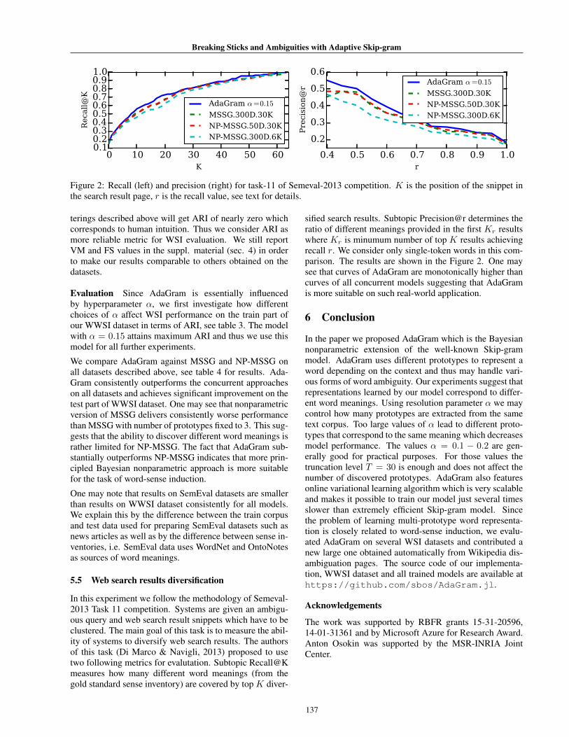
Figure 2: Recall (left) and precision (right) for task-11 of Semeval-2013 competition. K is the position of the snippet inthe search result page, r is the recall value, see text for details.

terings described above will get ARI of nearly zero whichcorresponds to human intuition. Thus we consider ARI asmore reliable metric for WSI evaluation. We still reportVM and FS values in the suppl. material (sec. 4) in orderto make our results comparable to others obtained on thedatasets.

Evaluation Since AdaGram is essentially influencedby hyperparameter ↵, we first investigate how differentchoices of ↵ affect WSI performance on the train part ofour WWSI dataset in terms of ARI, see table 3. The modelwith ↵ = 0.15 attains maximum ARI and thus we use thismodel for all further experiments.

We compare AdaGram against MSSG and NP-MSSG onall datasets described above, see table 4 for results. Ada-Gram consistently outperforms the concurrent approacheson all datasets and achieves significant improvement on thetest part of WWSI dataset. One may see that nonparametricversion of MSSG delivers consistently worse performancethan MSSG with number of prototypes fixed to 3. This sug-gests that the ability to discover different word meanings israther limited for NP-MSSG. The fact that AdaGram sub-stantially outperforms NP-MSSG indicates that more prin-cipled Bayesian nonparametric approach is more suitablefor the task of word-sense induction.

One may note that results on SemEval datasets are smallerthan results on WWSI dataset consistently for all models.We explain this by the difference between the train corpusand test data used for preparing SemEval datasets such asnews articles as well as by the difference between sense in-ventories, i.e. SemEval data uses WordNet and OntoNotesas sources of word meanings.

5.5 Web search results diversification

In this experiment we follow the methodology of Semeval-2013 Task 11 competition. Systems are given an ambigu-ous query and web search result snippets which have to beclustered. The main goal of this task is to measure the abil-ity of systems to diversify web search results. The authorsof this task (Di Marco & Navigli, 2013) proposed to usetwo following metrics for evalutation. Subtopic Recall@Kmeasures how many different word meanings (from thegold standard sense inventory) are covered by top K diver-

sified search results. Subtopic Precision@r determines theratio of different meanings provided in the first Kr resultswhere Kr is minumum number of top K results achievingrecall r. We consider only single-token words in this com-parison. The results are shown in the Figure 2. One maysee that curves of AdaGram are monotonically higher thancurves of all concurrent models suggesting that AdaGramis more suitable on such real-world application.

6 Conclusion

In the paper we proposed AdaGram which is the Bayesiannonparametric extension of the well-known Skip-grammodel. AdaGram uses different prototypes to represent aword depending on the context and thus may handle vari-ous forms of word ambiguity. Our experiments suggest thatrepresentations learned by our model correspond to differ-ent word meanings. Using resolution parameter ↵ we maycontrol how many prototypes are extracted from the sametext corpus. Too large values of ↵ lead to different proto-types that correspond to the same meaning which decreasesmodel performance. The values ↵ = 0.1 � 0.2 are gen-erally good for practical purposes. For those values thetruncation level T = 30 is enough and does not affect thenumber of discovered prototypes. AdaGram also featuresonline variational learning algorithm which is very scalableand makes it possible to train our model just several timesslower than extremely efficient Skip-gram model. Sincethe problem of learning multi-prototype word representa-tion is closely related to word-sense induction, we evalu-ated AdaGram on several WSI datasets and contributed anew large one obtained automatically from Wikipedia dis-ambiguation pages. The source code of our implementa-tion, WWSI dataset and all trained models are available athttps://github.com/sbos/AdaGram.jl.

Acknowledgements

The work was supported by RBFR grants 15-31-20596,14-01-31361 and by Microsoft Azure for Research Award.Anton Osokin was supported by the MSR-INRIA JointCenter.

137

Sergey Bartunov, Dmitry Kondrashkin, Anton Osokin, Dmitry P. Vetrov

ReferencesBlei, D. M. and Jordan, M. I. Variational inference for

Dirichlet process mixtures. Bayesian Analysis, 1:121–144, 2005.

Chen, D. and Manning, C. A fast and accurate dependencyparser using neural networks. In EMNLP, pp. 740–750,2014.

Chen, X., Liu, Z., and Sun, M. A unified model for wordsense representation and disambiguation. In EMNLP, pp.1025–1035, 2014.

Di Marco, Antonio and Navigli, Roberto. Clustering anddiversifying web search results with graph-based wordsense induction. Computational Linguistics, 39(3):709–754, 2013.

Ferguson, T. S. A Bayesian analysis of some nonparametricproblems. The Annals of Statistics, 1(2):209–230, 1973.

Hoffman, M. D., Blei, D. M., Wang, C., and Paisley, J.Stochastic variational inference. JMLR, 14(1):1303–1347, 2013.

Huang, E. H., Socher, R., Manning, C. D., and Ng, A. Y.Improving word representations via global context andmultiple word prototypes. In ACL, 2012.

Hubert, L. and Arabie, P. Comparing partitions. Journal ofclassification, 2(1):193–218, 1985.

Jordan, M. I., Ghahramani, Z., Jaakkola, T. S., and Saul,L. K. An introduction to variational methods for graphi-cal models. Machine Learning, 37(2):183–233, 1999.

Maas, A. L., Daly, R. E., Pham, P. T., Huang, D., Ng, A. Y.,and Potts, C. Learning word vectors for sentiment anal-ysis. In NAACL HLT, pp. 142–150, 2011.

Manandhar, S., Klapaftis, I. P., Dligach, D., and Pradhan,S. S. SemEval-2010 task 14: Word sense induction &disambiguation. In SemEval, pp. 63–68, 2010.

Mikolov, T., Sutskever, I., Chen, K., Corrado, G. S.,and Dean, J. Distributed representations of words andphrases and their compositionality. In NIPS, pp. 3111–3119, 2013a.

Mikolov, T., Yih, W., and Zweig, G. Linguistic regulari-ties in continuous space word representations. In NAACLHLT, pp. 746–751, 2013b.

Mnih, A. and Hinton, G. E. A scalable hierarchical dis-tributed language model. In NIPS, pp. 1081–1088, 2008.

Navigli, R. and Crisafulli, G. Inducing word senses to im-prove web search result clustering. In EMNLP, pp. 116–126, 2010.

Neelakantan, A., Shankar, J., Passos, A., and McCallum,A. Efficient non-parametric estimation of multiple em-beddings per word in vector space. In EMNLP, 2014.

Qiu, L., Cao, Y., Nie, Z., Yu, Y., and Rui, Y. Learning wordrepresentation considering proximity and ambiguity. InAAAI, pp. 1572–1578, 2014.

Reisinger, J. and Mooney, R. A mixture model with sharingfor lexical semantics. In EMNLP, pp. 1173–1182, 2010a.

Reisinger, J. and Mooney, R. J. Multi-prototype vector-space models of word meaning. In NAACL HLT, pp.109–117, 2010b.

Sethuraman, J. A constructive definition of Dirichlet priors.Statistica Sinica, 4:639–650, 1994.

Shaoul, C. and Westbury, C. The Westbury lab Wikipediacorpus. 2010.

Tian, F., Dai, H., Bian, J., Gao, B., Zhang, R., Chen, E.,and Liu, T.-Y. A probabilistic model for learning multi-prototype word embeddings. In COLING, pp. 151–160,2014.

Turian, J., Ratinov, L., and Bengio, Y. Word representa-tions: A simple and general method for semi-supervisedlearning. In ACL, pp. 384–394, 2010.

Vickrey, D., Biewald, L., Teyssier, M., and Koller, D.Word-sense disambiguation for machine translation. InEMNLP, 2005.

138