Brahms: Byzantine Resilient Random Membership Sampling

Edward Bortnikov∗ Maxim Gurevich∗ Idit Keidar∗ Gabriel Kliot†

Alexander Shraer∗

Abstract

We present Brahms, an algorithm for sampling random nodes ina large dynamic systemprone to Byzantine failures. Brahms stores small membership views at each node, and yetovercomes Byzantine failures of a linear portion of the system. Brahms is composed of twocomponents. The first one is a Byzantine-resistant gossip-based membership protocol. Thesecond one uses a novel memory-efficient approach for uniform sampling from a possibly bi-ased stream of ids that traverse the node. We evaluate Brahmsusing rigorous analysis, backedby extensive simulations, which show that our theoretical model captures the protocol’s essen-tials. We show that, with high probability, an attacker cannot create a partition between correctnodes. We further prove that each node’s sample converges toa uniform one over time. To ourknowledge, no such properties were proven for gossip-basedmembership in the past.

Keywords: random sampling, gossip, membership, Byzantine failures.

1Department of Electrical Engineering, The Technion – Israel Institute of Technology.Email: ebortnik@techunix, gmax@techunix, idish@ee, shralex@techunix.technion.ac.il.

2Department of Computer Science, The Technion – Israel Institute of Technology.Email: gabik@cs.technion.ac.il.

1 Introduction

We consider the problem of sampling a random node (or peer) ina large dynamic system subject to Byzan-tine (arbitrary) failures. Random node sampling is important for many scalable dynamic applications, in-cluding neighbor selection in constructing and maintaining overlay networks [13, 19, 22, 24], selection ofcommunication partners in gossip-based protocols [5, 8, 11], data sampling, and choosing locations for datacaching, e.g., in unstructured peer-to-peer networks [21].

Typically, in such applications, each node maintains a set of random node ids that is asymptoticallysmaller than the system size. This set is called alocal view. In a dynamic system, where the set of activenodes changes over time (this is calledchurn), the local views must continuously evolve to reflect thesechanges, adding new active nodes and removing ones that are no longer active. By using small local views,the maintenance overhead is kept small. In the absence of Byzantine failures, small local views can beeffectively maintained with gossip-based membership protocols [1, 11, 12, 16, 28], which were proven tohave a low probability for partitions, including under churn [1].

Nevertheless, Byzantine failures present a major challenge for small local views. Previous Byzantine-tolerant gossip protocols either considered static settings where the full membership is known to all [9, 20,26], or maintained (almost) full local views [3, 17], where faulty nodes cannot push correct ones out of theview. In contrast, small local views are susceptible to poisoning with entries (node ids) originating fromfaulty nodes; this is because the system is dynamic, and therefore nodes inherently must accept new idsand store them in place of old ones in their local views. It is even more challenging to provideindependentuniform samplesin such a setting. Even without Byzantine failures, gossip-based membership only ensuresthat eventually theaveragerepresentation of nodes in local views is uniform [1, 12, 16], and not thateverynodeobtains an independent uniform random sample. Faulty nodesmay attempt to skew the system-widedistribution, as well as the individual local view of a givennode.

In this paper, we address these challenges. We present Brahms (Section 3), a gossip-based membershipservice that stores a sub-linear number of ids (e.g.,Θ( 3

√N) in a system of sizeN ) at each node, and

provideseach nodewith membership samples that converge to uniform ones over time. The main ideasbehind Brahms are (1) to use gossip-based membership with some extra defenses to make it viable (in thesense that local views are not solely composed of faulty ids)in a Byzantine setting; (2) to recognize thatsuch a solution is bound to produce biased views due to attacks (we precisely quantify the extent of this biasmathematically); and (3) to correct this bias at each node.

To achieve the latter, we introduceSampler, a component that obtains uniform samples out of a datastream in which elements recur with an unknown bias, using min-wise independent permutations [6]. Weprove (Section 4) that Sampler obtains independent uniform samples from thebiased stream of gossipednode ids. By using suchhistory samplesof the gossiped ids to update part of the local view, Brahmsachievesself-healingfrom partitions that may occur with gossip-based membership. In particular, nodesthat have been active for sufficiently long (we quantify how long) cannot be isolated from the rest of thesystem. The use of history samples is an example ofamplification, whereby even a small healthy sample ofthe past can boost the resilience of a constantly evolving view. We note that only a small portion of the viewis updated with history samples, e.g.,10%. Therefore, the protocol can still deal effectively with churn.

One of the important contributions of this paper is our mathematical analysis (Section 5), which providesinsights to the extent of damage that Byzantine nodes can cause and the effectiveness of various mechanismsfor dealing with them. Extensive simulations of Brahms withup to4000 nodes validate the few simplifyingassumptions made in the analysis. We consider two possible goals for an attacker. First, we study attacksthat attempt to maximize the representation of faulty ids inlocal views at any given time. We show that as

1

long as faulty nodes comprise less than13 of the system, even without using history samples, the portion of

faulty ids in local views is bounded by a constant smaller than one. (Recall that the over-representation offaulty ids is later fixed by Sampler; the upper bound on faultyids in local views ensures Sampler has goodids to work with). If the adversary gains control of additional nodes after uniform samples have alreadybeen obtained, then Brahms can resistanyratio of faulty nodes.

Second, we consider an attacker that aims to partition the network. The easiest way to do so is byattempting to isolate one node from the rest. Clearly, once anode has obtained uniform samples of correctnodes, it can no longer be isolated. We therefore study an attack launched on a new node that joins thesystem when its samples are still empty, and when it does not yet appear in views or samples of other nodes.We further assume that such atargetedattack on the new node occurs in tandem with an attack on the entiresystem, as described above. The key to proving that Brahms prevents, w.h.p., an attacked node’s isolationis in comparing how long it takes for two competing processesto complete: on the one hand, we providea lower bound on the expected time to poison the entire view ofthe attacked node, assuming there are nohistory samples at all. On the other hand, we provide an uppper bound on how fast history samples areexpected to converge, under the same attack. Whenever the former exceeds the latter, the attacked nodeis expected to become immune to isolation before it is isolated. We prove that with appropriate parametersettings, this is indeed the case.

Finally, we simulate the complete system (Section 6), and measure Brahms’s resilience to the combi-nation of both attacks. Our results show that, indeed, Brahms prevents the isolation of attacked nodes, itsviews never partition, and the membership samples convergeto perfectly random ones over time.

Related Work. We are not familiar with prior work dealing with random node sampling in a Byzantinesetting. Previous Byzantine-tolerant membership services maintained full local views [17, 3] rather thanpartial samples. Previous work on gossip-based partial views [1, 11, 12, 16, 28], and on near-uniform nodesampling using random walks [13, 19, 23, 4] or DHT overlays [18] was limited to benign settings.

One application of Brahms is Byzantine-tolerant overlay construction. Brahms’s sampling allows eachnode to connect with some random correct nodes, thus constructing an overlay in which the sub-graphof correct nodes is connected. Several recent works, e.g., [27, 7, 2], have focused explicitly on securingoverlays, mostly structured ones, attempting to ensure that all correct nodes may communicate with eachother using the overlay, i.e., to prevent theeclipse attack[27], where routing tables of correct nodes aregradually poisoned with links to adversarial nodes. These works have a different focus than ours, since theirgoal is to construct (structured) overlay networks, whereas we present a general sampling technique, oneapplication of which is building Byzantine-resilient unstructured overlays.

2 Model and Required Properties

2.1 System Model

We consider a dynamic set of nodes, each of which can be eitheractiveor passiveat any given time. Eachnode is identified by a unique id, chosen when the node becomesactive for the first time. The set of activenodes at timet is denotedA(t). Active nodes can communicate through a fully connected network withreliable links. For simplicity of the analysis, we assume a synchronous model with a discrete global clock,zero processing times, and message latencies of a single time unit.

Some of the active nodes arecorrect, and the rest arefaulty. Faulty modes can exhibit arbitrary behavior(Byzantine faults). The subset of correct nodes inA(t) is denotedC(t). Nodes can determine the sourceof every message and cannot intercept messages addressed toother nodes (the standard ”unauthenticated“Byzantine model).In static systems (without churn), it is common to require that faulty nodes comprise less

2

than some fractionf < 1 of the nodes. In a dynamic setting, we require that the numberof faulty nodes atall times is limited by a constant fractionf of the minimal number of active nodes, i.e.,|⋃t(A(t) \ C(t))| ≤f ·mint|A(t)|.While this assumption rules out massive Sybil attacks [10] (by bounding the number of faultynode ids), it is weaker than assuming a certification authority [17], e.g., nodes can use historic informationfor choosing new active ids.

We assume a mechanism that makes it costly for nodes to send designated messages, which we calllimited messages, thereby limiting their sending rate. This mechanism can be implemented in differentways, e.g., computational challenges like Merkle’s puzzles [25], virtual currency, etc. We assume that thesystem-wide fraction of limited messages that all faulty nodes can jointly send in a single time unit is at mostp, for somep < 1. We also assume that the faulty nodes choose the destinations of all limited messages inadvance (i.e., they do not adapt their transmissions to information learned during the run).

2.2 Membership Sampling Specification

At all times t, Brahms provides two tuples at every active correct nodeu: a neighbor listNu(t) used forcommunication, and asample listSu(t). These lists may contain duplicates, and some entries inSu(t) maybe non-defined (denoted⊥). We denote thei’th element in the neighbor list and the sample list at timet byN i

u(t) andSiu(t), respectively. Every correct node has a limited local storage, asymptotically smaller than

the maximal size of the active node set (i.e., bothNu(t) andSu(t) are asymptotically smaller thanA(t)).First, we require the overlay induced byN to remain connected w.h.p.Formally, we define a dynamic

directedoverlay graph, which captures the knowledge of correct nodes about each other at each timet:

N (t) , C(t),⋃

u∈C(t)

(u, v)|v ∈ Nu(t) ∩ C(t).

Requirement 1 With high probability,N (t) remains weakly connected at allt.

Next, we requireS to converge to a uniform sample of the connected overlay. However, when the setof active nodes is constantly changing, the notion of a uniform distribution over it is meaningless. Hence,like previous specifications [1, 12, 16], we consider the system’s properties after a pointT0 when the churnof correct nodes ceases (i.e.,C(t) = C(T0) for all t ≥ T0). We are interested ineventual independentuniformsampling fromC(T0). Note that we cannot require the same from the set of faulty nodes, since theirbehavior is arbitrary. However, we require that (1) the probability of a sample being faulty does not exceedthe maximal fraction of faulty ids inA(t) afterT0, and (2) the probability of a sample being each specificcorrect id is eventually between1

|C(t)| and 1|A(t)| . Formally,

Requirement 2 If N (t) is weakly connected for allt ≥ T1 ≥ T0, then for allu, v ∈ C(T0), all samplesi,and all ε > 0, there existsTε ≥ T1 such that for allt ≥ Tε

1

maxT≥T0 |A(T )| − ε ≤ Pr[Siu(t) = v] ≤ 1

|C(T0)|+ ε.

In other words,1 − f

|C(T0)|− ε ≤ Pr[Si

u(t) = v] ≤ 1

|C(T0)|+ ε.

3

1: function Sampler.init()2: h← randomPRF(); q ← ⊥

3: function Sampler.next(elem)4: if q = ⊥ ∨ h(elem) < h(q) then5: q ← elem

6: function Sampler.sample()7: return q

Sampler Sampler Sampler Sampler

Id stream

sample()

next()

Validator

init()

Validator Validator Validator

Figure 1: Uniform sampling from an id stream in Brahms. (a) Sampler’s pseudo-code. (b) Sampling andvalidation of ℓ2 ids.

3 Brahms

Brahms has two components. The localsamplingcomponent maintains asample listS – a tuple of uniformsamples from the set of ids that traverse the node (Section 3.1). The gossipcomponent is a distributedprotocol that spreads locally known ids across the network (Section 3.2), and maintains a dynamicviewV.Each node has some initialV (e.g., received from some bootstrap server or peer node). The concatenationof V andS (denotedV S) is the node’sneighbor listN .

3.1 Sampling

Sampler is a building block for uniform sampling of unique elements from a data stream. The input streammay be biased, that is, some values may appear in it more than others. Sampler accepts one element at atime as input, produces one output, and stores a single element at any time. The output is a uniform randomchoice of one of the unique inputs witnessed thus far.

Sampler usesmin-wise independentpermutations [6]. A family of permutationsH over a range[1 . . . |U |]is min-wise independent if for any setX ⊂ [1 . . . |U |] and anyx ∈ X, if h is chosen at random fromH,thenPr(minh(X) = h(x)) = 1

|X| . That is, all the elements of any fixed setX have an equal chance tohave the minimum image underh. Pseudo-random (hash) functions (e.g., [14]) are considered an excellentpractical approximation of min-wise independent permutations, provided that|U | is large, e.g.,2160.

Sampler (Figure 1(a)) selects a random min-wise independent functionh upon initialization, and appliesit to all input values (next() function). The input with the smallest image value encountered thus farbecomes the output returned by thesample() function. The property of uniform sampling from the set ofunique observed ids follows directly from the definition of amin-wise independent permutation family.

Brahms maintains a tuple ofℓ2 sampled elements in a vector ofℓ2 Sampler blocks (Figure 1(b)), whichselect hashes independently. The same id stream is input to all Samplers. Sampled ids are periodicallyprobed (e.g., using pings), and a Sampler that holds an inactive node is invalidated (re-initialized).

3.2 Gossip

Brahms’s view is maintained by a gossip protocol (Figure 2). By slight abuse of notation, we denoteboth the vector of samplers and their outputs (the sample list) by S. Brahms executes in (unsynchronized)rounds. It uses two means for propagation: (1)push– sending the node’s id to some other node, and (2)pull– retrieving the view from another node. These operations serve two different purposes: pushes are requiredto reinforce knowledge about nodes that are under-represented in other nodes’ views (e.g., newborn nodes),whereas pulls are needed to spread existing knowledge within the network [1]. A combination of pulls and

4

1: V : tuple[ℓ1] of Id2: S : tuple[ℓ2] of Sampler3: N , V S

4: Initialization (V0):5: V ← V0

6: for all 1 ≤ i ≤ ℓ2 do7: S [i].init()8: updateSample(V0)

9: Stale sample invalidation10: periodically do11: for all 1 ≤ i ≤ ℓ2 do12: if probe(S [i].sample()) fails then13: S [i].init()

14: Auxiliary functions15: function updateSample(V)16: for all id ∈ V, 1 ≤ i ≤ ℓ2 do17: S [i].next(id)

18: function rand(V, n)19: return n random choices fromV

20: Gossip21: while true do22: Vpush ← Vpull ← ∅23: for all 1 ≤ i ≤ αℓ1 do24: Limited push25: send lim 〈“push request“〉 to rand(V, 1)26: for all 1 ≤ i ≤ βℓ1 do27: send 〈“pull request“〉 to rand(V, 1)

28: wait(1)

29: for all received 〈“push request“〉 from id do30: Vpush ← Vpush id31: for all received 〈“pull request“〉 from id do32: send 〈“pull reply“,V〉 to id

33: for all received 〈“pull reply“,V ′〉 from id do34: if I sent the request, and this is the first replythen35: Vpull ← Vpull V

′

36: if (|Vpush| ≤ αℓ1 ∧ Vpush 6= ∅ ∧ Vpull 6= ∅) then37: V ← rand(Vpush, αℓ1) rand(Vpull, βℓ1) rand(S , γℓ1)38: updateSample(Vpush Vpull)

Figure 2:The pseudo-code of Brahms.

αl1 βl1 γl1 l2

Pushed ids

Pulled ids

History samples

View SampleFigure 3:View re-computation in Brahms.

pushes is required because the representation of ids propagated solely by pulls decays over time, whereasthe representation of push-propagated ids increases.

Brahms uses parametersα > 0, β > 0 andγ > 0 that satisfyα + β + γ = 1. In a single round, acorrect node issuesαℓ1 push requests andβℓ1 pull requests to destinations randomly selected from its view(possibly with repetitions). At the end of each round,V andS are updated with fresh ids. While all receivedids are streamed toS (Figure 1, Line 38), re-computingV requires extra care, to protect against poisoningof the views with faulty ids. Brahms offers a set of techniques sto mitigate this problem.

Limited pushes. Since pushes arrive unsolicited, an adversary with an unlimited capacity could swampthe system with push requests. Then, correct ids would be propagated mainly through pulls, and theirrepresentation would decay exponentially [1]. Brahms employs limited push messages, hence the fractionof faulty pushes does not exceedp.

Attack detection and blocking. While using limited pushes prevents a simultaneous attack on all correctnodes, it provides no solace against an adversary that floodsa specific node. Brahms protects against thistargeted attackby blocking the update ofV. Namely, if more than the expectedαℓ1 pushes are received, itdoes not updateV. Although this policy slows down progress, its expected impact in the absence of attacksis bounded (nodes recomputeV in most rounds). Thanks to limited pushes, some nodes make progress evenunder an attack (Line 36).

Controlling the contribution of pushes vs pulls. As most correct nodes do not suffer from targeted attacks(due to limited pushes), their views are threatened by pullsfrom neighbors more than by adversarial pushes.

5

This is because whereas all pushes from correct nodes are correct, a pull from a random correct node maycontribute some faulty ids. Hence, the contribution of pushes and pulls toV must be balanced: pushes mustbe constrained to protect the targeted nodes, while pulls must be constrained to protect the rest. BrahmsupdatesV with randomly chosenαℓ1 pushed ids andβℓ1 pulled ids (Line 37).

History samples. The attack detection and blocking technique can slowdown a targeted attack, but notprevent it completely. Note that if the adversary succeeds to increase its representation in a victim’s viewthrough targeted pushes, it subsequently causes this victim to pull more data from faulty nodes. As theattacked node’s view deteriorates, it sends fewer pushes tocorrect nodes, causing its system-wide represen-tation to decrease. It then receives fewer correct pushes, opening the door for more faulty pushes1. Brahmsovercomes such attacks using a self-healing mechanism, whereby a portion (γ) of V reflects thehistory, i.e.,previously observed ids (Line 37). A direct use of history does not help since the latter may also be biased.Therefore, we use a feedback fromS to obtain unbiased history samples. Once some correct id becomesthe attacked node’s permanent sample (or the node’s id becomes a permanent sample of some other correctnode), the threat of isolation is eliminated.Figure 3illustrates the entire view re-computation procedure.

Brahms’s parameters entail a tradeoff between performancein a benign setting and resilience againstByzantine attacks. For example,γ must not be too large since the algorithm needs to deal with churn; onthe other hand, it must not be too small to make the feedback effective. We show (Section 6) thatγ = 0.1 isenough for protectingV from partitions. The choice ofℓ1 andℓ2 is crucial for guaranteeing that a targetedattack can be contained until the attacked node’s sample stabilizes. For example,ℓ1, ℓ2 = Θ( 3

√

|C(T0)|)suffice to protect even nodes that are attacked immediately upon joining the system (Section 5.2).

4 Analysis - Sampling

In this section we analyze the properties ofSu of a correct nodeu. Recall that each SamplerR employs amin-wise independent permutationR.h, chosen independently at random. LetR(t) be the output ofR attime t. We define theperfectid corresponding toR, VR ∈ A(T0), to be the id with the minimal value ofR.h in A(T0) (we neglect collisions for the sake of the definition). Note thatVR can be either a correct ora faulty id. InSection 4.1we show that the subset of correct ids inSu eventually converges to a uniformrandom sample fromC(T0). In Section 4.2we analyze how fast a node obtains at least one correct perfectsample, as needed for self-healing.Section 4.3discusses scalability, namely, how to choose view sizes thatensure a constant convergence time, independent of system size.

4.1 Eventual Convergence to Uniform Sample

Consider SamplerR. Given thatVR is correct,R samples correct ids uniformly at random. IfVR is faulty,it may refrain from answering pings and become invalidated instead of remaining in the sample. However,since faulty nodes do not adapt to the correct nodes’ random choices, we assume that such an invalidation isnot timed in order to capture any particular correct id intoR. We therefore assume that each correct id hasan equal probability for taking the place of an invalidated faulty node. The following theorem shows thatSu

satisfies Requirement 2 of the membership sampling specification (seeSection 2.2).

1This avalanche process can be started, e.g., by opportunistically sending the target a slightly higher number of pushesthanexpected. Since correct pushes are random, a round in which sufficiently few correct pushes arrive, such that Brahms doesnotdetect an attack, happens soon w.h.p.

6

Theorem 4.1 If N (t) remains weakly connected for eacht ≥ T1, for someT1 ≥ T0, then, for allv ∈ C(T0),andε > 0, there existsTε ≥ T1 such that for allt ≥ Tε

1 − f

|C(T0)|− ε ≤ Pr(R(t) = v) ≤ 1

|C(T0)|+ ε.

Proof idea (seeAppendix A.1). The key to the theorem is to show that wheneverN (t) remains weaklyconnected, the id of each correct node eventually reaches every other correct node w.h.p. This is becausethe id has a non-zero probability to traverse a path to every correct node in the system. Thus, each Samplerwill eventually settle on its perfect id, provided that its perfect id is correct. Therefore,Pr(R(t) = VR|VR ∈C(T0)) →t→∞ 1. Since the probability forVR to be faulty is at mostf , Pr(R(t) = VR) approaches therange[1− f, 1]. The theorem follows since∀v ∈ C(T0),Pr(R(t) = v|VR ∈ C(T0)) = 1

|C(T0)| , and since we

assume that whenVR is faulty,0 ≤ Pr(R(t) = v|VR /∈ C(T0)) ≤ 1|C(T0)| .

The next lemma discusses the convergence rate of samples.

Lemma 4.2 If no invalidations happen, for each correct nodeu, the expected fraction of Samplers thatoutput their perfect id grows linearly with the fraction of unique ids fromA(T0) observed byu.

Proof : LetD(t) ⊆ A(T0) be the set of ids observed byu until time t. Then, for each samplerR, Pr(VR ∈D(t)) = |D(t)|

|A(T0)| . Since for eachR such thatVR ∈ D(t), R(t′) = VR for t′ ≥ t, the lemma follows.

4.2 Convergence to First Perfect Sample

Here we analyze how many ids have to be observed by a correct node,u, in order to guarantee, w.h.p., thatits Su containsat least oneperfect id of an active correct node. This provides an upper bound on the time ittakesSu ensure self-healing and preventu’s isolation. We assume thatu joins the system at timeT0, withan empty sample. LetΛ(t) be the number of correct ids observed byu from timeT0 to t. Our analysisdepends on the number of unique ids observed byu, rather than directly onΛ. Obviously, one can expectthe observed stream to include many repetitions, as it is unrealistic to expect our gossip protocol to produceindependent uniform random samples (cf. [16]). Indeed, achieving this property is the goal of Sampler. Inorder to capture the bias inΛ, we define astream deficiency factor, 0 ≤ ρ ≤ 1, so that a stream of lengthΛ(t) produced by our gossip mechanism is roughly equivalent, forthe purposes of Sampler, to a stream oflengthρΛ(t) in which correct ids are independent and distributed uniformly at random. This is akin to theclustering coefficient of gossip-based overlays [16]. We empirically measuredρ to be about0.4 with ourgossip protocol (seeSection 5.2).

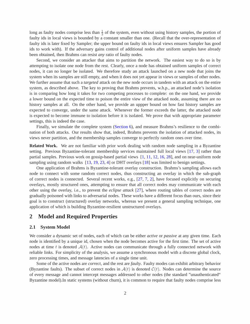
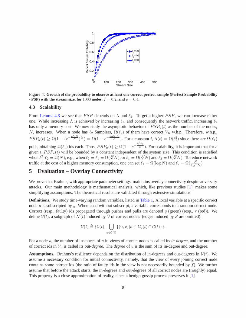
We define theperfect sample probabilityPSPu(t) as the probability thatSu(t) contains at least onecorrect perfect id. The convergence rate ofPSP is captured by the following:

Lemma 4.3 Letu be a random correct node. Then, fort > T0, PSPu(t) ≥ 1 − ((1 − f)e−

ρΛ(t)|C(T0)| + f)ℓ2 .

Proof idea (seeAppendix A.2). A Sampler outputs a correct perfect id if (1) its perfect id iscorrect, and(2) this id is observed by the Sampler in the stream.PSP is the probability that at least one ofℓ2 Samplersoutputs a correct perfect id.

Figure 4.2illustrates the dependence ofPSP on the stream sizeΛ(t) and onℓ2. When the sample sizeis 40 = 4 3

√

|A(T0)|, and the portion of unique ids in the stream isρ = 0.4, a perfect sample is obtained,w.h.p., after300 ids traverse the node.

7

0 100 200 300 400 5000

0.2

0.4

0.6

0.8

1

Stream SizeP

erfe

ct S

ampl

e P

roba

bilit

y

l2=20

l2=40

l2=60

Figure 4:Growth of the probability to observe at least one correct perfect sample (Perfect Sample Probability- PSP) with the stream size, for1000 nodes,f = 0.2, and ρ = 0.4.

4.3 Scalability

From Lemma 4.3we see thatPSP depends onΛ andℓ2. To get a higherPSP , we can increase eitherone. While increasingΛ is achieved by increasingℓ1, and consequently the network traffic, increasingℓ2has only a memory cost. We now study the asymptotic behavior of PSPu(t) as the number of the nodes,N , increases. When a node hasℓ2 Samplers,Ω(ℓ2) of them have correctVR w.h.p. Therefore, w.h.p.,

PSPu(t) ≥ Ω(1 − (e−ρΛ(t)

N )ℓ2) = Ω(1 − e−ρΛ(t)ℓ2

N ). For a constantt, Λ(t) = Ω(ℓ21) since there areΩ(ℓ1)

pulls, obtainingΩ(ℓ1) ids each. Thus,PSPu(t) ≥ Ω(1 − e−ℓ21·ℓ2

N ). For scalability, it is important that for agiven t, PSPu(t) will be bounded by a constant independent of the system size.This condition is satisfiedwhenℓ21 ·ℓ2 = Ω(N), e.g., whenℓ2 = ℓ1 = Ω( 3

√N), orℓ1 = Ω( 4

√N) andℓ2 = Ω( 2

√N). To reduce network

traffic at the cost of a higher memory consumption, one can setℓ1 = Ω(logN) andℓ2 = Ω( Nlog2 N

).

5 Evaluation – Overlay Connectivity

We prove that Brahms, with appropriate parameter settings,maintains overlay connectivity despite adversaryattacks. Our main methodology is mathematical analysis, which, like previous studies [1], makes somesimplifying assumptions. The theoretical results are validated through extensive simulations.

Definitions. We study time-varying random variables, listed inTable 1. A local variable at a specific correctnodeu is subscripted byu. When used without subscript, a variable corresponds to a random correct node.Correct (resp., faulty) ids propagated through pushes and pulls are denotedg (green) (resp.,r (red)). WedefineV(t), a subgraph ofN (t) induced byV of correct nodes: (edges induced byS are omitted):

V(t) , C(t),⋃

u∈C(t)

(u, v)|v ∈ Vu(t) ∩ C(t).

For a nodeu, the number of instances ofu in views of correct nodes is called itsin-degree, and the numberof correct ids inVu is called itsout-degree. Thedegreeof u is the sum of its in-degree and out-degree.

Assumptions. Brahms’s resilience depends on the distribution of in-degrees and out-degrees inV(t). Weassume a necessary condition for initial connectivity, namely, that the view of every joining correct nodecontains some correct ids (the ratio of faulty ids in the viewis not necessarily bounded byf ). We furtherassume that before the attack starts, the in-degrees and out-degrees of all correct nodes are (roughly) equal.This property is a close approximation of reality, since a benign gossip process preserves it [1].

8

Correct nodeu Random correct node Semantics

xu(t)/xu(t) x(t)/x(t) number/fraction of faulty ids in the view

yu(t)/yu(t) number/fraction of instances among the views of correct nodes

gpushu (t)/gpush

u (t) gpush(t)/gpush(t) number/fraction of correct ids pushed to the node

rpushu (t)/rpush

u (t) rpush(t)/rpush(t) number/fraction of faulty ids pushed to the node

gpullu (t)/gpull

u (t) gpull(t)/gpull(t) number/fraction of correct ids pulled by the node

rpullu (t)/rpull

u (t) rpull(t)/rpull(t) number/fraction of faulty ids pulled by the node

Table 1:Definition of common random variables.

Adversarial behavior. The adversary’s way to partition the overlay is through increasing its representationin the views of correct nodes. We assume the worst-case behavior by faulty nodes. In particular, they pushfaulty ids to correct nodes and always return faulty ids to pulls.

We first bound the damage that can be caused within asingleround (a similar approach was taken, e.g.,in [20]). In Appendix B, we proveLemma B.1, which asserts that in any single round, abalancedattack,which spreads faulty pushes evenly among correct nodes, maximizes the expected system-wide fraction offaulty ids, x(t), among all strategies. InSection 5.1, we prove that if this attack persists, the ratio of faultyids in the system eventually stabilizes at a fixed point. We study the convergence process, and show that forcertain parameter choices, this fixed point is strictly smaller than 1.

Alternatively, an adversary can try to partition the network (rather than increase its representation) bytargeting a subset of nodes with more pushes than in a balanced attack. Without prior information about theoverlay’s topology, attacking a single node can be most damaging, since the sets of edges adjacent to singlenodes are likely to be the sparsest cuts in the overlay.Section 5.2shows that had Brahms not used historysamples, correct nodes could have been isolated in this manner. However, Brahms sustains suchtargetedattacks, even if they start immediately upon a node’s join, when it is not represented in other views and hasno history. The key property is that Brahms’s gossip prevents isolation long enough for history samples tobecome effective.

Simulation setup. We validate our assumptions using simulations with N=1000 nodes or more. Each datapoint is averaged over 100 runs. The maximal possible numberof faulty nodes,fN , remain always active.For simplicity,p = f . A different subset of faulty nodes push their ids to a given correct node in each round,using a round-robin schedule. Faulty nodes always respond to probe requests, to avoid invalidation.

5.1 Balanced Attack

In the analysis of a balanced attack we ignore blocking sinceits only effect is to slow the convergencerate. Simulations show that this assumption has little effect on the results. Since a balanced attack does notdistinguish between correct nodes, we assume that it preserves the in-degrees and out-degrees of all correctnodes equal over time:

Assumption 5.1 For all u ∈ C(T0) and all t ≥ T0: xu(t) = x(t), andyu(t) = ℓ1 − xu(t).

We show the existence of a parameter-dependent fixed point ofx(t) and the system’s convergence to it.Since the focus is on asymptotic behavior, we assumet≫ T0.

Lemma 5.1 For t≫ T0, if p 6= 0 or x(t) 6= 1, the expected system-wide fraction of faulty ids evolves as

E(x(t+ 1)) = αp

p+ (1 − p)(1 − x(t))+ β(x(t) + (1 − x(t))x(t)) + γf.

9

!

(a) Impact of push

" "#$%&'()*+,$-* . #$%&'()*+,$-* /012345 67'' 89$:/;8&7'<=+)<>69$?&?)')<= @ABC01234DE567'' 89$:8&7'<=F$99*%< )- G&7'<= )-

(b) Impact of pull

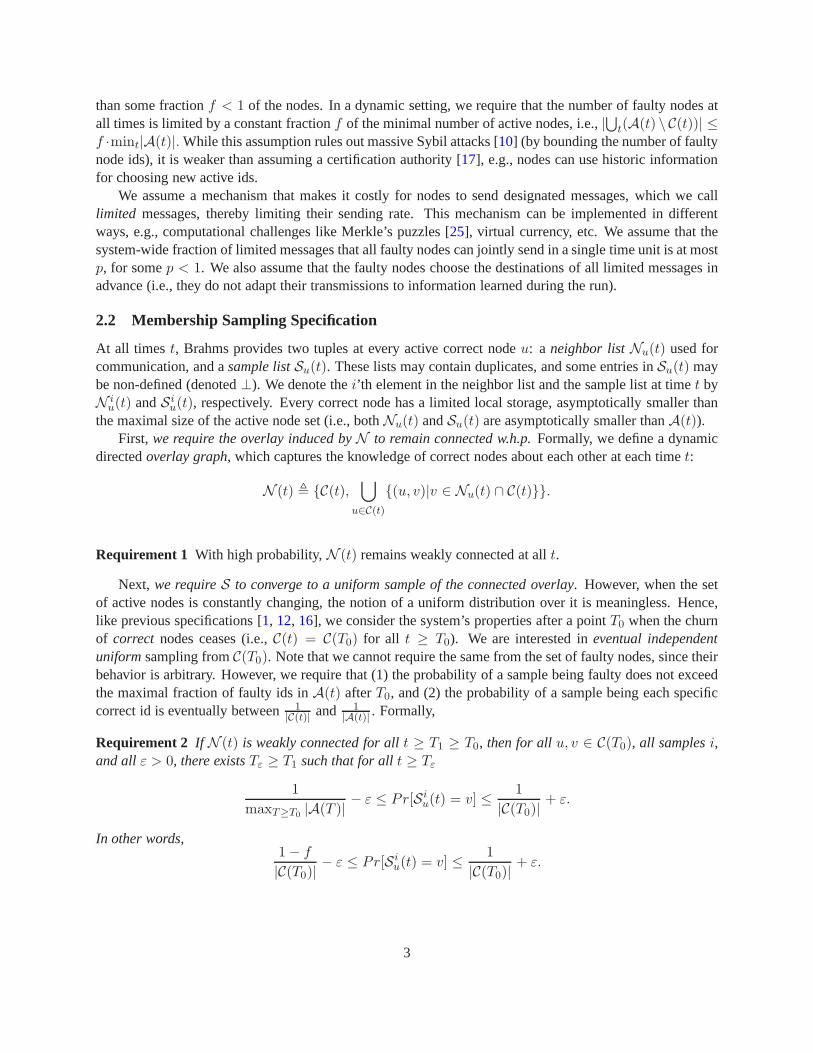
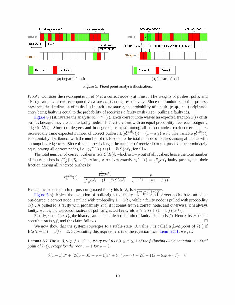
Figure 5:Fixed point analysis illustration.

Proof : Consider the re-computation ofV at a correct nodeu at timet. The weights of pushes, pulls, andhistory samples in the recomputed view areα, β andγ, respectively. Since the random selection processpreserves the distribution of faulty ids in each data source, the probability of a push- (resp., pull)-originatedentry being faulty is equal to the probability of receiving afaulty push (resp., pulling a faulty id).

Figure 5(a) illustrates the analysis ofrpush(t). Each correct node wastes an expected fractionx(t) of itspushes because they are sent to faulty nodes. The rest are sent with an equal probability over each outgoingedge inV(t). Since out-degrees and in-degrees are equal among all correct nodes, each correct nodeureceives the same expected number of correct pushes:E(gpush

u (t)) = (1 − x(t))αℓ1. The variablegpushu (t)

is binomially distributed, with the number of trials equal to the total number of pushes among all nodes withan outgoing edge tou. Since this number is large, the number of received correct pushes is approximatelyequal among all correct nodes, i.e.,gpush

u (t) ≈ (1 − x(t))αℓ1, for all u.The total number of correct pushes isαℓ1|C(T0)|, which is1−p out of all pushes, hence the total number

of faulty pushes ispαℓ11−p

|C(T0)|. Therefore,u receives exactlyrpushu (t) = p

1−pαℓ1 faulty pushes, i.e., their

fraction among all received pushes is:

rpushu (t) =

p1−p

αℓ1p

1−pαℓ1 + (1 − x(t))αℓ1

=p

p+ (1 − p)(1 − x(t)).

Hence, the expected ratio of push-originated faulty ids inVu is α pp+(1−p)(1−x(t)) .

Figure 5(b) depicts the evolution of pull-originated faulty ids. Since all correct nodes have an equalout-degree, a correct node is pulled with probability1 − x(t), while a faulty node is pulled with probabilityx(t). A pulled id is faulty with probabilityx(t) if it comes from a correct node, and otherwise, it is alwaysfaulty. Hence, the expected fraction of pull-originated faulty ids isβ(x(t) + (1 − x(t))x(t)).

Finally, sincet≫ T0, the history sample is perfect (the ratio of faulty ids in it isf ). Hence, its expectedcontribution isγf , and the claim follows.

We now show that the system converges to a stable state. A value x is called afixed pointof x(t) ifE(x(t+ 1)) = x(t) = x. Substituting this requirement into the equation fromLemma 5.1, we get:

Lemma 5.2 For α, β, γ, p, f ∈ [0, 1], every real root0 ≤ x ≤ 1 of the following cubic equation is a fixedpoint ofx(t), except for the rootx = 1 for p = 0:

β(1 − p)x3 + (2βp − 3β − p+ 1)x2 + (γfp− γf + 2β − 1)x+ (αp + γf) = 0.

10

0 0.2 0.4 0.6 0.8 10

0.5

1

1.5

Average ratio of faulty pushes (p)

Fix

ed−

poin

t ave

rage

rat

io o

f fau

lty id

s

Theoretical: α=β=0.5, γ=0Simulation: α=β= 0.5, γ=0, 1000 nodesTheoretical: α=β=0.45, γ=0.1Simulation: α=β= 0.45, γ=0.1, 1000 nodes

(a) Fixed pointx as a function ofp, for γ = 0 andγ > 0

0 5 10 15 20 25 300

0.1

0.2

0.3

0.4

0.5

0.6

0.7

0.8

Time

Fra

ctio

n of

faul

ty id

s in

the

view

Theory: 0% faulty ids in initial viewSimulation: 0% faulty ids in initial viewTheory: 20% faulty ids in initial viewSimulation: 20% faulty ids in initial viewTheory: 40% faulty ids in initial viewSimulation: 40% faulty ids in initial viewTheory: 60% faulty ids in initial viewSimulation: 60% faulty ids in initial viewTheory: 80% faulty ids in initial viewSimulation: 80% faulty ids in initial view

(b) Convergence tox: N = 1000, p = 0.2, α = β = 0.5 andγ = 0.

Figure 6: System-wide fraction of faulty ids in local views, under a balanced attack: (a) Fixed points (b)Convergence process.

If γ = 0 (no history samples),x = 1 is always a root. We call it atrivial fixed point. This is easilyexplainable, since if the views of all the correct nodes are totally poisoned, then neither pulls nor pusheshelp. Appendix Bshows that ifγ = 0, there can exist at most one nontrivial fixed point0 ≤ x < 1. For

example, ifα = β = 12 andγ = 0, thenx =

p+√

4p−3p2

2(1−p) , for 0 ≤ p ≤ 13 . In contrast, if the fraction of faulty

pushes exceeds13 , the only fixed point is 1, causing isolation of all correct nodes.If γ > 0, there exists a single nontrivial fixed point for allp. This highlights the importance of history

samples.Figure 6(a) depicts the analysis results, perfectly matched by simulations.We conclude the analysis by proving convergence to a nontrivial fixed point.

Lemma 5.3 If there exists a fixed pointx < 1 of x(t), andx(T0) < 1, thenx(t) converges tox.

Proof idea (seeAppendix B). We show that for allt, the sequence ofx(t) is trapped betweenx and anothersequence,φ(t), that converges tox. Hillam’s theorem [15] is then used to prove sequence convergence.

Since the balanced attack does not distinguish between correct nodes, the same result holds forxu(t),for each correct nodeu. Figure 6(b) depicts the convergence to the nontrivial fixed point from various initialvalues ofx(t). The analytical and simulation results are similar. The latter’s convergence is slightly slowerbecause the analysis ignores blocking.

5.2 Targeted Attack

We study a targeted attack on a single correct nodeu, which starts uponu’s join at T0. We prove thatu isnot isolated from the overlay by showing a lower bound on the expected time to isolation, which exceeds anupper bound on the time to a perfect correct sample (a sufficient condition for non-isolation,Section 4).

Lower bound on expected isolation time. As we seek a lower bound, we make a number of worst-caseassumptions (formally stated inAppendix C). First, we analyze a simplified protocol that does not employhistory samples (i.e.,γ = 0), so thatS does not correctV ’s bias. Next, we assume an unrealistic adaptiveadversary that observes the exact number of correct pushes to u, gpush

u (t), and complements them withαℓ1 − gpush

u (t) faulty pushes – the most that can be accepted without blocking. The adversary maximizesits global representation through a balanced attack on all correct nodesv 6= u, thus minimizing the fraction

11

of correct ids thatu pulls from correct nodes. Finally, we assume thatu is not represented in the systeminitially, and it derives its initial view from a random set of correct nodes, where the ratio of faulty ids is atthe fixed point (Section 5.1).

Clearly, the time to isolation inV(t) is a lower bound on that inN (t). We study the dynamics of thenumber of correct ids inu’s out-degree inV(t), ℓ1 − xu(t), andu’s in-degree,yu(t). We show that for anytwo specific values ofxu(t) andyu(t), the expected out-degree and in-degree values att+ 1 are

(

ℓ1 − E(xu(t+ 1))

E(yu(t+ 1))

)

=

(

β(1 − x) α

α 1−pp+(1−p)(1−x) β(1 − x)

)

×(

ℓ1 − xu(t)

yu(t)

)

.

Note that the coefficient matrix does not depend onxu(t) andyu(t), and the sum of entries in each row issmaller than 1. This implies that once the in-degree and the out-degree are close, they both decay exponen-tially. (Initially, this does not hold becauseu is not represented, i.e.,yu(T0) = 0.) Therefore, the expectedtime to isolation is logarithmic withℓ1. Note that this process does not depend on the number of nodes, sinceblocking bounds the potential attacks onu independently of the system-wide budget of faulty pushes. Hadblocking not been employed, the top right coefficient would have been0 instead ofα, because the adversarywould have completely hijacked the push-originated entries inVu. The decay factor would have been muchlarger, leading to almost immediate isolation.

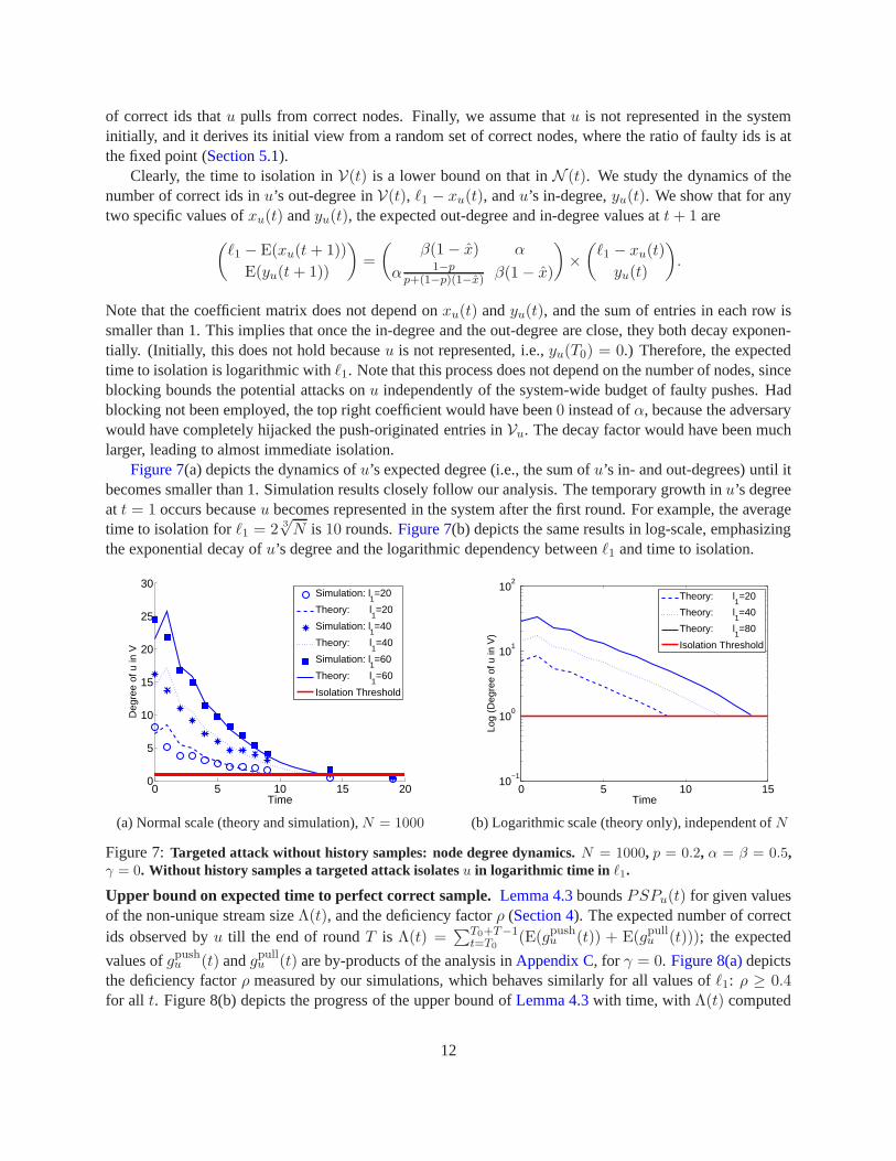
Figure 7(a) depicts the dynamics ofu’s expected degree (i.e., the sum ofu’s in- and out-degrees) until itbecomes smaller than 1. Simulation results closely follow our analysis. The temporary growth inu’s degreeat t = 1 occurs becauseu becomes represented in the system after the first round. For example, the averagetime to isolation forℓ1 = 2 3

√N is 10 rounds.Figure 7(b) depicts the same results in log-scale, emphasizing

the exponential decay ofu’s degree and the logarithmic dependency betweenℓ1 and time to isolation.

0 5 10 15 200

5

10

15

20

25

30

Time

Deg

ree

of u

in V

Simulation: l1=20

Theory: l1=20

Simulation: l1=40

Theory: l1=40

Simulation: l1=60

Theory: l1=60

Isolation Threshold

(a) Normal scale (theory and simulation),N = 1000

0 5 10 1510

−1

100

101

102

Time

Log

(Deg

ree

of u

in V

)

Theory: l1=20

Theory: l1=40

Theory: l1=80

Isolation Threshold

(b) Logarithmic scale (theory only), independent ofN

Figure 7:Targeted attack without history samples: node degree dynamics. N = 1000, p = 0.2, α = β = 0.5,γ = 0. Without history samples a targeted attack isolatesu in logarithmic time in ℓ1.

Upper bound on expected time to perfect correct sample.Lemma 4.3boundsPSPu(t) for given valuesof the non-unique stream sizeΛ(t), and the deficiency factorρ (Section 4). The expected number of correctids observed byu till the end of roundT is Λ(t) =

∑T0+T−1t=T0

(E(gpushu (t)) + E(gpull

u (t))); the expected

values ofgpushu (t) andgpull

u (t) are by-products of the analysis inAppendix C, for γ = 0. Figure 8(a)depictsthe deficiency factorρ measured by our simulations, which behaves similarly for all values ofℓ1: ρ ≥ 0.4for all t. Figure 8(b) depicts the progress of the upper bound ofLemma 4.3with time, withΛ(t) computed

12

0 5 10 15 200

0.2

0.4

0.6

0.8

1

Time

Str

eam

siz

e

Simulation: l1=20

Simulation: l1=40

Simulation: l1=60

(a) Deficiency factor

0 5 10 15 200

0.2

0.4

0.6

0.8

1

Time

Per

fect

Sam

ple

Pro

babi

lity

Simulation: l1=l

2=20

Theory: l1=l

2=20

Simulation: l1=l

2=40

Theory: l1=l

2=40

Simulation: l1=l

2=60

Theory: l1=l

2=60

(b) Perfect sample probability

Figure 8: Dynamics within a targeted node (N = 1000, p = 0.2, α = β = 0.5 and γ = 0): (a) Fraction ofunique ids in the stream of correct ids,ρ. (b) Growth of Perfect Sample Probability (PSP) with time,ρ = 0.4.PSP becomes high quickly enough to prevent isolation.

as explained above andρ = 0.4. The corresponding simulation results show, for each timet, the fractionof runs in which at least one correct id inSu is perfect. Forℓ2 ≥ 40, the PSP becomes close to 1 in a fewrounds, much faster than isolation happens (Figure 7(b)). Forℓ1 = 20, it stabilizes at0.5. The growth stopsbecause we run the protocol without history samples, thusu becomes isolated, and the id stream ceases.A higher PSP can be achieved by independently increasingℓ2, e.g., if ℓ2 is 40, then the PSP grows to0.8(Figure 4.2). Note that perfect samples only provide an upper bound on self-healing time, asSu containsimperfect correct ids, andu also becomes sampled by other correct nodes, w.h.p. These factors coupled withhistory samples (γ > 0) completely preventu’s isolation, as shown inSection 6.

6 Putting it All Together

In previous sections we analyzed each of Brahms’s mechanisms separately. We now simulate the entiresystem.Figure 9depicts the degree of nodeu in N (t) under a targeted attack. Nodeu remains connectedto the overlay, thanks to history samples (γ = 0.1). Note that the actual degree ofu in N (t) is higher thanthe lower bound shown inSection 5.2, due to the pessimistic assumptions made in the analysis (nohistorysamples, no imperfect correct ids, etc.).

0 20 40 60 800

20

40

60

80

100

Time

Deg

ree

of u

in th

e N

eigh

bour

Lis

t

Simulation: l1=20

Simulation: l1=40

Simulation: l1=60

Figure 9:Degree dynamics of an attacked node inN (t),N = 1000, p = 0.2, α = β = 0.45 and γ = 0.1.

13

0 50 100 150 2000

0.2

0.4

0.6

0.8

1

Time

Fra

ctio

n of

per

fect

sam

ple

N=1000N=2000N=3000N=4000

(a) Perfect samples vs time

0 50 100 1500

0.05

0.1

0.15

0.2

0.25

0.3

0.35

0.4

Time

Fra

ctio

n of

faul

ty id

s

N=1000N=2000N=3000N=4000Expected

(b) Faulty ids vs. time

Figure 10:Fraction of (a) perfect samples and (b) faulty nodes inS, under a balanced attack (f = 0.2), for1000, 2000, 3000 and 4000 nodes,ℓ2 = 2 3

√N .

We now demonstrate the convergence ofS in the correct nodes. We simulate systems with up toN =4000 nodes;ℓ1 andℓ2 are set to2 3

√N . To measure the quality of sampleS under a balanced attack, we depict

the fraction of ids inS that are indeed the perfect sample over time (Figure 10(a)). Note that this criterion isconservative, since missing a perfect sample does not automatically lead to a biased choice. More than50%of perfect samples are achieved within less than 15 rounds; for ℓ2 = ℓ1 = 3 3

√N , the convergence is twice as

fast.Figure 10(b)depicts the evolution of the fraction of faulty ids inS. Initially, this fraction equalsf , andat first increases, up to approximately the fixed point’s value. This is to be expected, since the first observedsamples are distributed like the original (biased) data stream. Subsequently, as the node encounters moreunique ids, the quality ofS improves, and the fraction of faulty ids drops fast tof . The protocol exhibitsalmost perfect scalability, as the convergence rate is the same forN ≥ 2000.

7 Conclusions

We presented Brahms, a Byzantine-resilient membership sampling algorithm. Brahms stores small views,and yet resists the failure of a linear portion of the nodes. It ensures that every node’s sample converges toa uniform one, which was not achieved before by gossip-basedmembership even in benign settings. Wepresented extensive analysis and simulations explaining the impact of various attacks on the membership,as well as the effectiveness of the different mechanisms Brahms employs.

Acknowledgments

We thank Christian Cachin for his valuable suggestions thathelped to improve our paper. We are grateful toRoie Melamed and Igor Yanover for fruitful discussions of a random walk overlay-based solution.

References

[1] A. Allavena, A. Demers, and J. E. Hopcroft. Correctness of a gossip based membership protocol. InACMPODC, pages 292–301, 2005.

[2] B. Awerbuch and C. Scheideler. Towards a Scalable and Robust DHT. InSPAA, pages 318–327, 2006.

[3] G. Badishi, I. Keidar, and A. Sasson. Exposing and Eliminating Vulnerabilities to Denial of Service Attacks inSecure Gossip-Based Multicast. InDSN, pages 201–210, June – July 2004.

14

[4] Z. Bar-Yossef, R. Friedman, and G. Kliot. RaWMS - Random Walk based Lightweight Membership Service forWireless Ad Hoc Networks. InACM MobiHoc, pages 238–249, 2006.

[5] K. P. Birman, M. Hayden, O. Ozkasap, Z. Xiao, M. Budiu, andY. Minsky. Bimodal multicast.ACM Transactionson Computer Systems, 17(2):41–88, 1999.

[6] A. Z. Broder, M. Charikar, A. M. Frieze, and M. Mitzenmacher. Min-wise independent permutations.J. Com-puter and System Sciences, 60(3):630–659, 2000.

[7] T. Condie, V. Kacholia, S. Sankararaman, J. Hellerstein, and P. Maniatis. Induced Churn as Shelter from Rout-ingTable Poisoning. InNDSS, 2006.

[8] A. Demers, D. Greene, C. Hauser, W. Irish, J. Larson, S. Shenker, H. Sturgis, D. Swinehart, and D. Terry.Epidemic Algorithms for Replicated Database Management. In ACM PODC, pages 1–12, August 1987.

[9] D.Malkhi, Y. Mansour, and M. K. Reiter. On Diffusing Updates in a Byzantine Environment. InSymposium onReliable Distributed Systems, pages 134–143, 1999.

[10] J.R. Douceur. The Sybil Attack. InIPTPS, 2002.

[11] P. Th. Eugster, R. Guerraoui, S. B. Handurukande, P. Kouznetsov, and A.-M. Kermarrec. Lightweight proba-bilistic broadcast.ACM Transactions on Computer Systems (TOCS), 21(4):341–374, 2003.

[12] A. J. Ganesh, A.-M. Kermarrec, and L. Massoulie. SCAMP:Peer-to-Peer Lightweight Membership Service forLarge-Scale Group Communication. InNetworked Group Communication, pages 44–55, 2001.

[13] C. Gkantsidis, M. Mihail, and A. Saberi. Random walks inpeer-to-peer networks. InIEEE INFOCOM, 2004.

[14] O. Goldreich, S. Goldwasser, and S. Micali. How to construct random functions.JACM, 33(4):792–807, 1986.

[15] B. P. Hillam. A Generalization of Krasnoselski’s Theorem on the Real Line.Math. Mag., 48:167–168, 1975.

[16] M. Jelasity, S. Voulgaris, R. Guerraoui, A.-M. Kermarrec, and M. van Steen. Gossip-based peer sampling.ACMTrans. Comput. Syst., 25(3):8, 2007.

[17] H. Johansen, A. Allavena, and R. van Renesse. Fireflies:scalable support for intrusion-tolerant network overlays.In Proc. of the 2006 EuroSys conference (EuroSys), pages 3–13, 2006.

[18] V. King and J. Saia. Choosing a random peer. InACM PODC, pages 125–130, 2004.

[19] C. Law and K. Siu. Distributed construction of random expander networks. InIEEE INFOCOM, April 2003.

[20] H. C. Li, A. Clement, E. L. Wong, J. Napper, I. Roy, L. Alvisi, and M. Dahlin. BAR Gossip. InProc. of the 7thUSENIX Symposium on Operating Systems Design and Implementation (OSDI), pages 45–58, November 2006.

[21] C. Lv, P. Cao, E. Cohen, K. Li, and S. Shenker. Search and replication in unstructured peer-to-peer networks. InProc. of the 16th International Conference on Supercomputing (ICS), pages 84–95, 2002.

[22] G. Manku, M. Bawa, and P. Raghavan. Symphony: Distributed hashing in a small world. InProc. of the 4thUSENIX Symposium on Internet Technologies and Systems (USITS), 2003.

[23] L. Massoulie, E. Le Merrer, A.-M. Kermarrec, and A. J. Ganesh. Peer Counting and Sampling in OverlayNetworks: Random Walk Methods. InACM PODC, pages 123–132, 2006.

[24] R. Melamed and I. Keidar. Araneola: A Scalable ReliableMulticast System for Dynamic Environments. InIEEE NCA, pages 5–14, 2004.

[25] R. C. Merkle. Secure Communications over Insecure Channels.CACM, 21:294–299, April 1978.

[26] Y. M. Minsky and F. B. Schneider. Tolerating Malicious Gossip.Dist. Computing, 16(1):49–68, February 2003.

[27] Atul Singh, T.-W. Ngan, Peter Druschel, and Dan S. Wallach. Eclipse Attacks on Overlay Networks: Threatsand Defenses. InIEEE INFOCOM, 2006.

[28] S. Voulgaris, D. Gavidia, and M. van Steen. CYCLON: Inexpensive Membership Management for UnstructuredP2P Overlays.Journal of Network and Systems Management, 13(2):197–217, July 2005.

15

A Analysis - sampling

A.1 Eventual convergence

Proposition A.1 If N (t) remains weakly connected for eacht ≥ T1 for someT1 ≥ T0 then, for eachu, v ∈ C(T0), there is a positive probability ofv ∈ Vu(t′i) for infinitely many timest′i > T1.

Proof : For t ≥ T1, we define the(t)-reachable setof u, denotedΓu(t), as a set of correct ids that havenonzero probability to appear inVu(t‘), for someT1 ≤ t‘ ≤ t. Clearly,Γu(T1) = Vu(T1)

⋂ C(T0), andΓu(t) ⊆ Γu(t + 1), for all t ≥ T1. We show that as long asΓu(t) ⊂ C(T0), the setΓu(t) grows by atleast one correct id each three rounds. For simplicity we consider a slightly transformed protocol that doesnot employ blocking. The only effect of this is a faster, by a constant factor, growth rate ofΓu. Note thatv ∈ Γu(t) impliesPr(v ∈ Vu(t′)) > 0 for all t′ ≥ t, asv can remain inVu indefinitely, e.g., by repeatedlyexchanging withu push messages, or ifv is sampled byu into Su and then returned by the history samplingmechanism toVu.

A new entry inVu(t) can appear following (1) a push from some other nodev, (2) pulling a view fromsome other nodev, and (3) applying a history sample fromSu(t). Let us define the effects of these threeoperations as following:Γu(t) = Γu(t− 1)

⋃

∆(t)⋂ C(T0), where

∆(t) = ∆push(t)⋃

∆pull(t)⋃

∆history(t)

is the set of nodes that can potentially reachVu(t). We now describe each of its components.

∆push(t) = v|u ∈ Vv(t− 1)⋃

v|Γu(t− 2) ∩ Vv(t− 2) 6= ∅⋃

v|Γu(t− 3) ∩ Sv(t− 3) 6= ∅

is a set of to all the node ids that can potentially reachu through push. Note that only the first term refersto the direct pushes tou. The second term refers to pushes to some intermediate nodew ∈ Γu(t − 2),that can then be pulled byu. The second term refers to the nodes that first sample some intermediate nodew ∈ Γu(t− 3) from their history sample, then push tow, and only then their ids can be pulled byu fromw.

∆pull(t) =⋃

v∈Γu(t)

Vv(t− 1)

is a set of to all the nodes thatu can potentially pull from.

∆history(t) = Su(t− 1)

is a set of to all the nodes thatu can potentially sample from its history sample.Recall thatN (t) is a directed graph spanned by(Vv(t)

⋃Sv(t))⋂ C(t) of all correct nodesv. Since

N (t) is connected, for any subset ofC(T0), in particularΓu(t), there exist at least one edge between thatsubset and the complementing subset. Consider a nodev ∈ C(T0) \Γu(t), connected to somew ∈ Γu(t) byan edge inN (t). It is easy to see thatv will appear in either∆(t + 1), ∆(t + 2), or ∆(t + 3), dependingonw and the origins of the edge (e.g., on whetherw = u, whether the edge originated fromVu or SU , etc.).Therefore, for at least each third roundt, ∆(t)

⋂

Γu(t) 6= ∅, andΓu(t) is a proper superset ofΓu(t − 1),which guarantees that byt = T1 + 3|C(T0)|, Γu(t) will contain all the nodes inC(T0).

We have shown that by the timeT1 + 3|C(T0)|, all ids inC(T0) have a positive probability to appear inVu between timeT1 andT1 + 3|C(T0)|. Obviously, we can start over and see that after the next period of

16

3|C(T0)| rounds all ids inC(T0) had a chance to appear inVu, and so on. We conclude that afterT1, each idin C(T0) can appear inVu infinitely many times.

The following proposition shows that each correct perfect id VR can eventually be observed byR, sothat there exist timet, such thatR(t) = VR.

Proposition A.2 If N (t) remains weakly connected for eacht ≥ T1 for someT1 ≥ T0 then, for eachVR ∈ C(T0)

limt→∞

Pr(R(t) = VR|VR ∈ C(T0)) = 1.

Proof : Let nodeu be the owner ofR. It follows from Proposition A.1that the probability ofVR appear inVu, and consequently inu’s stream approaches1. The proposition follows immediately.

W assume that each correct id has equal probability to take place of an invalidated faulty id in a Sampler.

Assumption A.1 In each SamplerR, such thatVR /∈ C(T0), for eachv ∈ C(T0) and for eacht > T0,

0 ≤ Pr(R(t) = v|VR /∈ C(T0)) ≤1

|C(T0)|.

The assumption is justified since the if faulty nodeVR responds to all invalidation probes,Pr(R(t) =v) = 0, and if it never responds to them,Pr(R(t) = v) = 1

|C(T0)| . Otherwise, if it sometimes does andsometimes does not, since faulty nodes do not adapt to the local choices of correct nodes, no correct id willbe overrepresented compared to the other correct nodes.

Theorem 4.1(restated) If N (t) remains weakly connected for eacht ≥ T1, for someT1 ≥ T0, then, forall v ∈ C(T0), andε > 0, there existsTε ≥ T1 such that for allt ≥ Tε

1 − f

|C(T0)|− ε ≤ Pr(R(t) = v) ≤ 1

|C(T0)|+ ε.

Proof : We can writePr(R(t) = v) as following:

Pr(R(t) = v) = Pr(R(t) = v|VR ∈ C(T0)) · Pr(VR ∈ C(T0))

+ Pr(R(t) = v|VR /∈ C(T0)) · Pr(VR /∈ C(T0)).

FromProposition A.2we know thatlimt→∞ Pr(R(t) = VR|VR ∈ C(T0)) = 1, so that

limt→∞

Pr(R(t) = v|VR ∈ C(T0)) = Pr(VR = v|VR ∈ C(T0)) =1

|C(T0)|.

From here, for eachε > 0, there existsTε ≥ T1 such that for allt ≥ Tε,

1

|C(T0)|− ε ≤ Pr(R(t) = v|VR ∈ C(T0)) ≤

1

|C(T0)|+ ε.

Using AssumptionA.1, and sincePr(VR ∈ C(T0)) ≥ 1−f andPr(VR ∈ C(T0)) ≤ f , we boundPr(R(t) =v) as following. For allε > 0, there existsTε ≥ T1 such that for allt ≥ Tε

1 − f

|C(T0)|− ε ≤ Pr(R(t) = v) ≤ 1

|C(T0)|+ ε.

17

A.2 Convergence rate

In the following lemma we study the dependency between the probability of a sampler to output a correctperfect id and the numberΛ(t) of correct ids observed by the Sampler, and the stream deficiency factorρ.

Proposition A.3 For |C(T0)| ≫ 1 and for eacht > T1, for someT1 ≥ T0,

Pr(R(t) = VR|VR ∈ C(T0)) = 1 − e−

ρΛ(t)|C(T0)| .

Proof : Sampler outputs its perfect idVR only after that id passed in the Sampler’s input stream. So theprobability ofR(t) 6= VR is the probability thatVR did not appear in the stream of during the roundsT0 ≤ t′ ≤ t. Denote elementj (considering only the correct ids) in the input stream ofR byG(j), and notethat for eachv ∈ C(T0), Pr(G(j) = v) = 1

|C(T0)| . Then,

Pr(R(t) 6= VR|VR ∈ C(T0)) = Pr(VR /∈ρΛ(t)⋃

j=1

G(j)|VR ∈ C(T0)) =

ρΛ(t)∏

j=1

Pr(G(j) 6= VR|VR ∈ C(T0)) =

ρΛ(t)∏

j=1

(1 − Pr(G(j) = VR|VR ∈ C(T0))) =

ρΛ(t)∏

j=1

(

1 − 1

|C(T0)|

)

=

(

1 − 1

|C(T0)|

)ρΛ(t)

.

Since 1|C(T0)|

≪ 1, we can rely on1 − x ≈ e−x for x≪ 1 and approximate the above as following

Pr(R(t) 6= VR|VR ∈ C(T0)) ≈(

e− 1

|C(T0)|

)ρΛ(t)

= e− ρΛ(t)

|C(T0)| .

From now on, we assume 1|C(T0)| is small enough, so we use equality. It is now obvious that

Pr(R(t) = VR|VR ∈ C(T0)) = 1 − e− ρΛ(t)

|C(T0)| .

Lemma 4.3(restated) Letu ∈ C(T0) be a random correct node. Then, fort > T0,

PSPu(t) ≥ 1 −(

(1 − f)e− ρΛ(t)

|C(T0)| + f

)ℓ2

.

Proof : Sinceℓ2 of u’s Samplers are independent, the probability of each one to have a correct perfect id is

Pr(VR ∈ C(T0)) =|A(T0)

⋂ C(T0)||A(T0)|

≥ 1 − f.

18

Similarly,

Pr(VR /∈ C(T0)) =|A(T0) \ C(T0)|

|A(T0)|≤ f.

Based onProposition A.3, the probability ofR(t) not being a correct perfect id is

Pr(R(t) 6= VR ∨ VR /∈ C(T0)) = Pr(R(t) 6= VR|VR ∈ C(T0)) Pr(VR ∈ C(T0)) + Pr(VR /∈ C(T0))

≤ (1 − f)e−

ρΛ(t)|C(T0)| + f.

We now calculate the perfect sample probabilityPSPu(t), which equals1 minus the probability of each ofℓ2 Samplers not outputting a correct perfect id.

PSPu(t) = 1 −ℓ2∏

i=1

Pr(R(t) 6= VR ∨ VR /∈ C(T0)) =

1 − (Pr(R(t) 6= VR ∨ VR /∈ C(T0)))ℓ2 ≥

1 −(

(1 − f)e−

ρΛ(t)|C(T0)| + f

)ℓ2

.

B Balanced Attack Analysis

B.1 Short-term Optimality

We now prove that in any single round, a balanced attack maximizes the expected system-wide fraction offaulty ids, x(t), among all strategies. Consider a scheduleR : C(T0) → N that assigns a number of faultypushes to each correct node at roundt. A schedule isbalancedif for every two correct nodesu andv, itholds that|R(u) − R(v)| ≤ 1. Otherwise, the schedule isunbalanced. We prove that every unbalancedschedule is suboptimal. All balanced schedules are equallyoptimal, for symmetry considerations.

Lemma B.1 If scheduleR is unbalanced, then there exists another schedule that imposes a larger expectedratio of faulty ids thanR in roundt+ 1.

Proof : Since a schedule of faulty pushes in roundt does not affect the pulls in this round, it is enough toprove the claim for the push-originated ids. Consider two nodes,u andv, such thatR(u) > R(v) + 1.Consider an alternative scheduleR′ that differs fromR in moving a single push fromu to v. Consider thechange in the expected cumulative fraction of push-originated faulty ids inVu(t + 1) andVv(t + 1) afterthis shift (in the other nodes, the ratio of faulty ids does not change).

The probability of a push-originated view entry at nodeu being faulty, provided thatR(u) faulty pusheswere received, is equal to the expected fraction ofR(u) among all pushes received byu. Note thatR(u) isset in advance, i.e., without knowing the number of receivedcorrect pushes,gpush

u (t) (Section 2.1). Condi-tioning on the latter, we get:

E(rpushu |rpush

u = R(u)) =

|C(T0)|∑

G=1

Pr[gpushu (t) = G] · R(u)

R(u) +G.

19

We need to show that

E(rpushu |rpush

u = R(u)−1)+E(rpushv |rpush

v = R(v)+1) > E(rpushu |rpush

u = R(u))+E(rpushv |rpush

v = R(v)),

i.e.,|C(T0)|∑

G=1

Pr[gpushu (t) = G] · R(u) − 1

R(u) − 1 +G+

|C(T0)|∑

G=1

Pr[gpushv (t) = G] · R(v) + 1

R(v) + 1 +G

≥|C(T0)|∑

G=1

Pr[gpushu (t) = G] · R(u)

R(u) +G+

|C(T0)|∑

G=1

Pr[gpushv (t) = G] · R(v)

R(v) +G.

Since all correct nodes have the same in-degree inV(t) (Assumption 5.1), gpushu (t) andgpush

v (t) have iden-tical (binomial) distributions. Hence, it is enough to showthat

R(u) − 1

R(u) − 1 +G+

R(v) + 1

R(v) + 1 +G≥ R(u)

R(u) +G+

R(v)

R(v) +G,

for all G ≥ 0 and allR(u) > R(v) + 1 > 0. We start simplifying:

−G(R(u) −G)(R(u) − 1 +G)

+G

(R(v) +G)(R(v) + 1 +G)≥ 0.

SinceR(u) − 1 ≥ R(v) + 1 > 0,

−G(R(u) +G)(R(u) − 1 +G)

+G

(R(v) +G)(R(v) + 1 +G)

≥ −G(R(u) +G)(R(u) − 1 +G)

+G

(R(u) − 2 +G)(R(u) − 1 +G)

≥ G

R(u) − 1 +G· [ 1

R(u) − 2 +G− 1

R(u) +G] =

G

R(u) +G· 2

(R(u) +G)(R(u) − 2 +G)> 0.

We conclude by showing that all balanced schedules are equally optimal for the adversary.

Proposition B.2 Every two balanced schedules induce the same expected fraction of faulty ids in roundt+ 1.

Proof : R can be transformed intoR′ by a sequence of moves of a single push message from nodeu tonodev, such thatR(u) = R(v) + 1 whereasR′(v) = R′(u) + 1. For symmetry reasons, neither of thesemoves alters the expected cumulative fraction of faulty idsreceived byu andv. Hence, each transformationproduces a schedule that implies the samex(t+ 1) as the previous one.

20

−0.4 −0.2 0 0.2 0.4 0.6 0.8 1 1.2−0.15

−0.1

−0.05

0

0.05

0.1

0.15

0.2

0.25

xg(

x)

p=0.5p=0.25p=0

Figure 11:Nontrivial fixed points x (depicted by circles), forα = β = 1

2, γ = 0.

B.2 Fixed Point Analysis

Fixed point values. Considerg(x) , β(1−p)x3+(2βp−3β−p+1)x2+(γfp−γf+2β−1)x+αp+γf .By Lemma 5.2, the fixed pointx is a root ofg(x). Note thatg(0) = (α+ γ)p > 0, andg(1) = p(α + β +γp − 1) ≤ 0. Hence, ifγ > 0, then the function has a single feasible rootx ∈ (0, 1) (the others lie outside[0, 1]). In other words, there is always a single nontrivial fixed point. If γ = 0, thenx = 1 is always a root(a trivial fixed point). Since there exists an infeasible negative root, this leaves room for at most one moreroot 0 ≤ x < 1 (i.e., theremayexist at most one nontrivial fixed point).Figure 11depicts the behavior ofg(x) for α = β = 1

2 (γ = 0), and different values ofp. The fixed points are depicted by circles.Two more parameter combinations deserve special interest:

1. β = 1, α = γ = 0 (pull only, no history samples). The only valid root isx = 0, for all p. That is, ifnone of the views initially contain a faulty id, and the faulty nodes cannot push their own ids, then thelatter will remain unrepresented.

2. α = 1, β = γ = 0 (push only, no history samples). The only valid root isx = p1−p

, for p ≤ 12 .

That is, a nonzero fraction of correct ids can be maintained iff the majority of pushes are correct. Thisfollows from the fact that a single correct push and a single faulty push equally contribute to the view.

Convergence. We prove convergence to a nontrivial fixed point.

Lemma 5.3(restated) If there exists a fixed pointx < 1 of x(t), andx(T0) < 1, thenx(t) converges tox.

Proof : We defineψ(x) : [0, 1] → [0, 1] asψ(x) , α pp+(1−p)(1−x) +β(x+(1− x)x)+γf . The sequence of

expected values ofx(t) is defined by the iteration schemex(t+ 1) = ψ(x(t)), for t ≥ T0. We show thatfor any x(T0) < 1, this scheme converges tox. For this purpose, we define an auxiliary sequenceφ(t)that converges tox, such that for eacht, the value ofx(t) is trapped betweenx andφ(t), thus implying thedesired result.

A straightforward calculus shows two facts to be used throughout the proof:

1. ψ(x) is monotonically increasing forx ∈ [0, 1], since both pp+(1−p)(1−x) andx+ (1− x)x = 2x− x2

are monotonically increasing in this interval.

21

2. The absolute value of the first derivative ofψ(x) for x ∈ [0, 1] is bounded by a constantK (except fora combinationp = 0, x = 1 which we do not consider).

By the mean value theorem, for allx1, x2 ∈ [0, 1] (x1 ≤ x2), there existsx′ ∈ [x1, x2] such that

ψ(x2) − ψ(x1) =δψ

δx(x′) · (x2 − x1).

Hence, the function satisfies the Liphschitz condition withconstantK, namely, for each pairx1, x2 ∈ [0, 1],it holds that|ψ(x1) − ψ(x2)| ≤ K|x1 − x2|. Therefore, by Hillam’s theorem [15], the iteration schemeφ(t + 1) = λφ(t) + (1 − λ)ψ(φ(t)), whereλ = 1

K+1 , converges to a fixed point ofψ(x) for eachφ(T0) ∈ [0, 1]. It remains to show that the sequencex(t) is confined betweenx andφ(t), and therefore,it also converges tox. Specifically, we argue that:

1. Assume thatx < x(T0) = φ(T0) < 1. Then, (a) the sequenceφ(t) converges tox, and (b) for allt ≥ T0, it holds thatx < x(t) ≤ φ(t).

2. Assume that0 ≤ x(T0) = φ(T0) < x. Then, (a) the sequenceφ(t) converges tox, and (b) for allt ≥ T0, it holds thatφ(t) ≤ x(t) < x.

We prove the first part of the claim (the second part’s proof issymmetrical). Recall thatx is a singlenontrivial fixed point. By the definition,x is the root of the functionψ(x) − x, which is negative forx ∈ (x, 1) (i.e., ψ(x) < x). For an arbitraryx ∈ (x, 1), it holds thatλx + (1 − λ)ψ(x) < x, i.e, thesequenceφ(t) is monotonically decreasing witht. Hence, this sequence cannot converge to the trivialfixed point (if one exists), i.e., it converges tox.

Next, we prove thatx < x(t) ≤ φ(t) by induction ont. The basis is immediate. Assume thatx < x(t) ≤φ(t) for somet ≥ T0. We denoteX , x(t) andΦ , φ(t). It holds thatφ(t+ 1) = λΦ + (1 − λ)ψ(Φ) >ψ(Φ). Sinceψ(x) is a monotonically increasing function forx ∈ [0, 1], ψ(Φ) ≥ ψ(X) = x(t+ 1), that is,φ(t+ 1) > x(t+ 1). Similarly, x(t+ 1) = ψ(X) > ψ(x) = x, thus concluding the induction step.

C Targeted Attack Analysis

This section analyzes the dynamics of a targeted attack on a single correct node, which aims isolating itfrom the other correct nodes.

C.1 Assumptions

We use the following assumptions on the environment to boundthe time to isolation from below.

Assumption C.1 (no history samples)γ = 0, which is equivalent to the worst-case assumption that theexpected ratio of faulty ids inS at all times is equal to that in the id stream observed by the node (i.e.,history samples are ineffective).

Assumption C.2 (unrealistically strong adversary) In each roundt ≥ T0, the adversary observes the exactnumber of correct pushes received byu, gpush

u (t), and complements it with faulty pushes toαℓ1 (i.e., themaximal number of faulty ids that can be accepted without blocking). Formally,rpush

u (t) , max(αℓ1 −gpushu (t), 0).

22

Assumption C.3 (background attack on the rest of the system) The adversary maximizes its global rep-resentation through a balanced attack on all correct nodesv 6= u. At timeT0, the system-wide expectedfraction of faulty ids is at the fixed pointx. (Note that this attack minimizes the fraction of correct ids thatucan pull from correct nodes).

Assumption C.4 (fresh attacked node)u joins the system atT0. It is initially not represented in any correctnode’s view andu’s initial view is taken from a random correct node.

We assume that the effect ofu on the entire system’s dynamics is negligible. Hence, we assume thatthe out-degrees and the in-degrees of all correct nodes except u are equal at all times (Assumption 5.1), andthese nodes do not block (Section 5.1showed that the system-wide effect of blocking is marginal).

C.2 Node Degree Dynamics

We study the dynamics of the degree of the attacked nodeu V(t). Consider a set of triples(X,Y, t), eachstanding for a statexu(t) = X ∧ yu(t) = Y , for X ∈ 0, . . . , ℓ1, Y ∈ 0, . . . , |C(T0)|ℓ1. Eachtdefines a probability space, i.e.,

∑

X,Y Pr[(X,Y, t)] = 1. Sinceu is initially not represented, the only statesthat have non-zero probability fort = T0 are those for whichY = 0. The probability distribution over thesestates is identical to the distribution ofxu(T0). Sinceu borrows its initial view from a random collection ofcorrect nodes,xu(T0) ∼ Bin(ℓ1, x).

We now develop probability spaces for eacht > T0. The notationPr[(X ′, Y ′, t + 1)|(X,Y, t)] standsfor the probability of transition from state(X,Y, t) to state(X ′, Y ′, t). That is,Pr[(X ′, Y ′, t + 1)] =∑

X,Y Pr[(X ′, Y ′, t + 1)|(X,Y, t)] · Pr[(X,Y, t)]. To analyzePr[(X ′, Y ′, t + 1)|(X,Y, t)] we separatelyconsider four independent random variables: the number of push- and pull-originated entries inVu, (denotedxpushu (t) andxpullu (t)), and the number of push- and pull-propagated instances ofu in the views of correct

nodes (denotedypushu (t) andypullu (t)). The first two affectX ′ whereas the last two affectY ′. We nowdemonstrate how conditional probability distributions for these variables are computed. For convenience,we omit the conditioning on(X,Y, t) from further notation.

ypullu (t): Since the system is at the fixed point, the probability of pulling from some other correct node

is (1 − x). Hence,ypullu (t + 1) is a binomially distributed variable, with the number of trials equal to thetotal number of correct pulls,(1 − x)βℓ1|C(T0)|, and the probability of success equal to the chance of anentry in a random node’s view beingu, namely Y

ℓ1|C(T0)|: ypullu (t+ 1) ∼ Bin((1 − x)βℓ1|C(T0)|, Y

ℓ1|C(T0)|).

Note thatE(ypullu (t+ 1)) = β(1 − x)Y .

ypushu (t): By Lemma 5.1, the number of pushes that reach correct nodes isαℓ1|C(T0)| (1−x)(1−p)+p

1−p.

Denote the number of pushes fromu to correct nodes in roundt by zu(t). This is a binomially distributedvariable withαℓ1 trials and probability of success equal to1 − X

ℓ1: zu(t) ∼ Bin(αℓ1, 1 − X

ℓ1). For a given

zu(t) = Z, since the total number of push-originated entries isαℓ1|C(T0)|, the number of push-propagatedinstances ofu is ypushu (t+ 1|Z) ∼ Bin (αℓ1|C(T0)|, Z

αℓ1|C(T0)|((1−x)+ p1−p

)). Note thatE(y

pushu (t+ 1|Z)) =

Z 1−pp+(1−p)(1−x) . Hence, sinceZ is independent onp andx,

E(ypushu (t+ 1)) = E(Z)1 − p

p+ (1 − p)(1 − x)= α(ℓ1 −X) · 1 − p

p+ (1 − p)(1 − x).

xpullu (t): A pull from a faulty node (which happens with probabilityX

ℓ1) produces a faulty id with

probability 1, otherwise the probability to receive a faulty id is x. Hence, the probability of pulling a faulty

23

id is Xℓ1

+ (1 − Xℓ1

)x. That is, the number of pull-originated faulty ids inu’s view is xpullu (t + 1) ∼Bin(βℓ1,

Xℓ1

+ (1 − Xℓ1

)x) (i.e.,E(xpullu (t+ 1)) = β(X + (ℓ1 −X)x)).

We also compute the expected number of correct ids (with duplicates) pulled byu, which we need forestimating the size of the id stream that traverses this node(Section 5.2). Sinceu performsβℓ1 pulls, andthe expected number of correct ids pulled from a random node is (1 − x)ℓ1,

E(gpullu (t)) = (1 − X

ℓ1) · βℓ1 · (1 − x)ℓ1 = (1 − x)ℓ1(ℓ1 −X).

xpushu (t): The number of push-originated ids,xpushu (t + 1), depends on the number of correct pushes

received byu, gpushu (t). The latter is a binomially distributed variable, with the number of trials equal to

the total number of correct pushes,αℓ1|C(T0)|, and the probability of success equal to the chance of anentry in a random node’s view beingu, namely Y

ℓ1|C(T0)|: gpush

u (t) ∼ Bin(αℓ1|C(T0)|, Yℓ1|C(T0)|

) (Note that

E(gpushu (t)) = αY . This value is of independent use for evaluating the size of the id stream that traversesu

(Section 5.2)).An expected representation of a correct node different fromu in the system is(1 − x)ℓ1. Sinceu is

under-represented (Y < (1 − x)ℓ1 w.h.p), the probability of receiving aboveαℓ1 correct pushes is low, andhence, we ignore the case ofu being blocked by exceedingly many correct pushes. On the other hand, faultypushes cannot blocku either (AssumptionC.2), and therefore, we assume thatu never blocks. IfG ≤ αℓ1correct pushes are received, the adversary complements thenumber of pushes to the maximum allowed(AssumptionC.2), i.e., the fraction of faulty pushes tou is 1 − G

αℓ1. Hence, the number of push-originated

faulty ids inu’s view isxpushu (t+ 1|G) ∼ Bin(αℓ1, 1 − Gαℓ1

). In other words,

E(xpushu (t+ 1)) = αℓ1(1 − E(gpushu (t))

αℓ1) = αℓ1(1 − αY

αℓ1) = α(ℓ1 − Y ).

Putting it all together. Summing up, the expected values of in-degree and out-degreecan be written as(

ℓ1 − E(xu(t+ 1))

E(yu(t+ 1))

)

=

(

ℓ1 − (E(xpushu (t+ 1)) + E(x

pullu (t+ 1)))

E(ypushu (t+ 1)) + E(y

pullu (t+ 1))

)

=

=

(

ℓ1 − (α(ℓ1 − Y ) + β(X + (ℓ1 −X)x))

α(ℓ1 −X) 1−pp+(1−p)(1−x) + β(1 − x)

)

=

=

(

β(1 − x) α

α 1−pp+(1−p)(1−x) β(1 − x)

)

·(

ℓ1 − xu(t)

yu(t)

)

Since we have shown thatu does not block w.h.p., andSection 5.1demonstrated that the effect of blockingon the rest of correct nodes is negligible, we assume that allviews are recomputed in each round. That is,

Pr[xu(t+ 1) = X ′|(X,Y, t)] =∑

X′1+X′

2=X′

Pr[xpushu (t) = X ′1|(X,Y, t)] · Pr[xpullu (t) = X ′

2|(X,Y, t)],

and

Pr[yu(t+ 1) = Y ′|(X,Y, t)] =∑

Y ′1+Y ′

2=Y ′

Pr[ypushu (t) = Y ′1 |(X,Y, t)] · Pr[ypullu (t) = Y ′

2 |(X,Y, t)].

Since the computations ofX ′ andY ′ are independent, we conclude:

Pr[(X ′, Y ′, t)|(X,Y, t)] = Pr[xu(t+ 1) = X ′|(X,Y, t)] · Pr[yu(t+ 1) = Y ′|(X,Y, t)].

24