Boundary Conditions for Direct Simulations of...

JOURNAL OF COMPUTATIONAL PHYSICS 101, 104- 129 ( 1992)

Boundary Conditions for Direct Simulations of Compressible Viscous Flows

T. J. POINSOT*

Center for Turbulence Research, Stanford University, Stanford, California 94305

AND

S. K. LELE+

NASA Ames Research Center, Moffett Field, California 94305

Received February 23, 1990; revised April 12, 1991

Procedures to define boundary conditions for Navier-Stokes equations are discussed. A new formulation using characteristic wave relations through boundaries is derived for the Euler equations and generalized to the Navier-Stokes equations. The emphasis is on deriving boundary conditions compatible with modern non-dissipative algorithms used for direct simulations of turbulent flows. These methods have very low dispersion errors and require precise boundary conditions to avoid numerical instabilities and to control spurious wave reflections at the computational boundaries. The present formulation is an attempt to provide such conditions. Reflecting and non-reflecting boundary condition treatments are presented. Examples of practical implementations for inlet and outlet boundaries as well as slip and no-slip walls are presented. The method applies to subsonic and supersonic flows. It is compared with a reference method based on extrapolation and partial use of Riemann invariants. Test cases described include a ducted shear layer, vortices propagating through boundaries, and Poiseuille flow. Although no mathematical proof of well-posedness is given, the method uses the correct number of boundary conditions required for well-posedness of the Navier-Stokes equations and the examples reveal that it provides a significant improvement over the reference method. 0 1992 Academic Press, Inc.

CONTENTS

1. Introduction. 2. Description of characteristic boundary conditions for Navier-

Stokes equations. 2.1. Principle of the method. 2.2. The Navier- Stokes equations for a reacting flow. 2.3. The local one- dimensional inviscid (LODI) relations. 2.4. The NSCBC strategy for Euler equations. 2.5. The NSCBC strategy for Navier-Stokes equations. 2.6. The treatment of edges and corners.

* Present affiliation: Laboratoire EM2C, C.N.R.S., Ecole Centrale de Paris, Chatenay-Malabry 92295 Cedex, France.

+ Departments of Mechanical Engineering and Aero and Astro, Stanford University, Stanford, California 94305.

3. Examples of implementation. 3.1. A subsonic inflow. 3.2. A subsonic non-reflecting outflow. 3.3. A subsonic reflecting outflow. 3.4. An isothermal no-slip wall. 3.5. An adiabatic slip wall. 3.6. An adiabatic no-slip wall.

4. Applications to steady non-reacting flows. 5. Applications to reactingjlows. 6. Applications to unsteady flows. 7. Applications to low Reynolds number flows: The Poiseuillejlow. 8. Conclusions.

1. INTRODUCTION

Direct simulations of Navier-Stokes equations have been the focus of many recent studies. In the field of finite difference methods, modern algorithms based on high-order schemes can provide spectral-like resolution and very low numerical dissipation (Thompson [l], Lele [a]). The precision and the potential applications of these schemes, however, are constrained by the boundary conditions which have to be included in the final numerical models. Most direct simulations are performed with periodic boundary conditions. In these configurations, the reference frame moves at the mean flow speed and flow periodicity is assumed. This is the only geometry for which the problem can be closed exactly at the boundary: by assuming periodicity, the computation domain is folded on itself and no boundary conditions are actually required. The periodicity assumption considerably limits the possible applications of these simulations. Simulations in which no periodicity is assumed and flow inlets and outlets must be treated are much less common. Indeed, these simulations are strongly dependent on boundary conditions and on their treatment and general boundary conditions for direct simulations of compressible flows are needed. The new

0021~9991/92 S5.00 Copyright 0 1992 by Academic Press, Inc. All rights of reproduction in any form reserved.

104

BOUNDARY CONDITIONS FOR NAMER-STOKES 105

constraints imposed on boundary condition formulations by these unsteady computations performed with high-order numerical methods in non-periodic domains are the following:

l Direct simulation of compressible flows requires an accurate control of wave reflections from the boundaries of the computational domain. This is not the case when Navier-Stokes codes are used only to compute steady states. In these situations waves have to be eliminated and one is not interested in the behavior of boundaries as long as a final steady state can be obtained. It is worth noting that the mechanisms by which waves (especially acoustic waves) are eliminated in many codes is somewhat unclear and very often due to numerical dissipation. As direct simulation algorithms strive to minimize numerical viscosity, acoustic waves have to be eliminated by another mechanism such as better non-reflecting or absorbing boundary conditions.

l A large amount of experimental evidence suggests that acoustic waves are strongly coupled to many mechanisms encountered in turbulent flows. The initial instability as well as the growth of non-reacting shear layers are sensitive to acoustic waves (Bechert and Stahl [203). This interaction may even lead to large flow instabilities as, for example, in the case of the edgetone experiment (Ho and Nosseir [21], Tang and Rockwell [22]). In the field of reacting flows, combustion instabilities provide numerous examples of interactions between turbulent combustion and acoustic waves (Yu et al. [S], Poinsot et al. [4], Poinsot and Candel [23], Sterling and Zukoski [S]). The simulation of these phenomena requires an accurate control of the behavior of the computation boundaries. Many studies have been concerned with direct simulation of combustion instabilities (Menon and Jou [6], Kailasanath et al. [7]) but the iden- tification of the acoustical behavior of boundaries is not explicit and its effects on the results are unclear. The problem of the downstream boundary is often removed by considering supersonic outlets where all variables are obtained by extrapolation. Even in cases where physical waves are not able to propagate upstream from the outlet, numerical waves may do so and interact with the flow. For example, recent studies show that strong numerical coupling mechanisms between inlet and outlet boundaries can lead to non-physical oscillations for the one-dimensional advection equation (Vishnevetsky and Pariser [30]).

l Although exact boundary conditions ensuring well- posedness can be derived for Euler equations (Kreiss [S], Higdon [9], Engquist and Majda [lo], Gustafsson and Oliger [ 11 I), the problem is much more complex for Navier-Stokes equations. Determining if a given set of boundary conditions applied to Navier-Stokes equations will lead to a well-posed problem can only be assessed in certain simple cases (Gustafsson and Sundstriim [12],

Oliger and Sundstriim [ZS]). Although the recent work of P. Dutt [29] gives a general method to check the well- posedness of Navier-Stokes equations and some examples of implementations, it covers only a small part of the practical questions related to this problem. The existence of acoustic waves crossing the boundaries, for example, is not considered.

l Discretization and implementation of boundary conditions require more than the knowledge of the conditions ensuring well-posedness of the original Navier-Stokes equations. Other conditions have to be added to the original set of boundary conditions to solve for variables which are not specified by the boundary conditions. These additional conditions are often called “numerical” boundary conditions although they should be viewed only as compatibility relations required by the numerical method and not as boundary conditions. The computational results depend not only on the original equations and the boundary conditions but also on the numerical scheme and on the numerical conditions used at the boundaries.

The objective of this paper is to use recent theoretical results on well-posedness of Navier-Stokes boundary conditions to construct a systematic method for specifying these boundary conditions. This method has been derived using the following criteria:

(1) It reduces to Euler boundary conditions when the viscous terms vanish. The method presented here is an extension of recent methods developed for hyperbolic equations (Thompson [ 11) and is valid for Euler and Navier-Stokes equations. It allows control of the different waves which cross the boundaries.

(2) It does not use any extrapolation procedure, thereby suppressing the arbitrariness in the construction of the boundary conditions.

(3) The number of boundary conditions specified for Navier-Stokes equations is that obtained by theoretical analysis of well-posedness (Strikwerda [33], Dutt [29]).

The method presented here is certainly not the only solution for boundary conditions for Navier-Stokes equations, Other modern methods to specify boundary conditions may be found, for example, in Dutt [29], Rudy [39], Lowery et al. [40], or Grinstein et al. [26]. The limitations of our approach, suggested by theoretical considerations or evidenced through practical applications, will also be described. However, test results and comparisons with other methods support this formulation and show its precision and robustness. The present method was originally derived for direct simulations of turbulent reacting flows and a complete description of the method for such flows may be found in Poinsot and Lele [38].

Section 2 will describe the theory behind the method and

106 POINSOT AND LELE

its implementation for Euler and Navier-Stokes equations. Section 3 will provide examples of implementation for different boundary conditions (subsonic inflow and outflow, non-reflecting boundaries, slip wall, no-slip wall). Section 4 will concentrate on some test results for stationary flows. Section 5 will give examples of applications for unsteady flows. Finally, Section 6 will provide examples of viscous flow computations at low Reynolds number (Poiseuille flow).

2. DESCRIPTION OF CHARACTERISTIC BOUNDARY CONDITIONS FOR NAVIER-STOKES EQUATIONS

2.1. Theory of the Method

An appealing technique for specifying boundary conditions for hyperbolic systems is to use relations based on characteristic lines, i.e., on the analysis of the different waves crossing the boundary. This method has been extensively studied for the Euler equations [l, 2, 8, 9, lo]. The objectives of this work are to construct such a method for the Euler equations and then to extend this analysis to the Navier-Stokes equations. Although our main concern is direct simulation of turbulent flows, the method is also well suited to low Reynolds number flows. Such a method will be called Navier-Stokes characteristic boundary conditions (NSCBC) (although it is clear that the concept of “characteristic lines” may be questionable for the Navier-Stokes equations). The NSCBC method is valid for Navier-Stokes and Euler equations and relaxes smoothly from one to the other when the viscosity goes to zero.

The reader is referred to the papers of Kreiss [S] or Engquist and Majda [9] for a description of the mathematical background of boundary conditions based on characteristic wave analysis. Different levels of complexity may be incorporated in these methods. For example, some of the variables on the boundaries can be extrapolated while some others are obtained from a partial set of characteristic relations (Rudy and Strikwerda [14, 151, Grinstein et al. [26], Yee [ 171). However, it seems reasonable to avoid any kind of extrapolation (Moretti [ 161). We will describe how this can be done first for the Euler equations (Section 2.4) and emphasize modifications required for the Navier- Stokes equations (Section 2.5). The following presentation is focused on explicit finite difference algorithms but can be easily extended to other numerical methods (e.g., finite elements, implicit finite differences, etc.).

Before describing the method we must introduce some terminology. Boundary condition treatments may be very different and some confusion between the nature of the conditions (physical vs numerical) is found in the literature. Two classes of boundary conditions may be distinguished:

TABLE I

Number of Physical Boundary Conditions Required for Well-Posedness (Three-Dimensional Flow)

Boundary type Euler Navier-Stokes

Supersonic inflow Subsonic inflow Supersonic outflow Subsonic outflow

5 5 4 5 0 4 1 4

(1) We will call a boundary condition a physical boundary condition when it specifies the known physical behavior of one or more of the dependent variables at the boundaries. For example, specification of the inlet longitudinal velocity on a boundary is a physical boundary condition. These conditions are independent of the numerical method used to solve the relevant equations. We expect the number of necessary and sufficient physical boundary conditions to be that suggested by theoretical analysis (Oliger and Sundstrom [28], Dutt [29], Strikwerda [32]), as summarized in Table I for a three-dimensional flow. To build Navier-Stokes boundary conditions, the approach used in the NSCBC method is to take conditions corresponding to Euler conditions (the inviscid conditions) and to supply additional relations (the “viscous” conditions) which refer to viscous or diffusion effects. The term “viscous” is used here to describe all processes which are specific to Navier-Stokes, i.e., viscous dissipation and thermal diffusion. For example, a three dimensional viscous subsonic outflow requires four “physical” boundary conditions (Strikwerda [ 321): one of them will be the inviscid relation obtained for Euler equations and it will be complemented by three “viscous” conditions. We will see (Section 2.5) that the NSCBC procedure follows Strikwerda’s results in all cases except two: the subsonic inlet with imposed temperature and velocities and the supersonic outlet.

(2) Knowing which physical boundary conditions to impose is not enough to solve the problem numerically. When the number of physical boundary conditions is less than the number of primitive variables (this is always the case at an outflow), how can we find the variables which are not specified? The usual method is to introduce “soft” (or “numerical”) conditions. We will consider a boundary condition to be “soft” when no explicit boundary condition fixes one of the dependent variables, but the numerical implementation requires us to specify something about this variable. Soft boundary conditions have often been called “numerical” boundary conditions because they appear to be needed for the numerical method while not being explicitly given by the physics of the problem (Yee [ 173). The methods to treat soft conditions can be divided into two groups:

BOUNDARY CONDITIONS FOR NAVIER-STOKES 107

l Arbitrary conditions may be added to the physical boundary conditions to obtain the missing dependent variables on the boundary. Many authors use extrapolation for variables which are not imposed by one of the physical boundary conditions. For example, fixing the velocity and the temperature at the inlet of a one-dimensional duct for an inviscid flow computations comprises two “physical” boundary conditions which require a “soft” boundary condition for the inlet pressure if the flow is subsonic. Extrapolation of pressure using pressure values at interior points may be used (Grinstein et al. [26], Yee [17]), but the compatibility of these methods with the original set of physical boundary conditions is unclear. Extrapolation acts as an additional physical condition imposing a zero pressure gradient and therefore overspecifies the boundary conditions.

l A more rigorous method is to use the conservation equations themselves on the boundary to complement the set of physical boundary conditions. It is the approach used in the present work. Variables which are not imposed by physical boundary conditions are computed on the boundaries by solving the same conservation equations as in the domain. In the previous example of a one-dimensional subsonic inlet, pressure will be found in the NSCBC method by using the energy conservation equation on the boundary itself.

Four difficulties are associated with the NSCBC approach for soft boundary conditions:

(1) Near the boundaries, the accuracy of the spatial derivatives has to be decreased. Typically, centered differences have to be replaced by one-sided differences because grid points are available only on the interior side of the boundary. Theoretical approaches (Gustafsson [ 37 J) and tests (Lele [2]) indicate that this is not a major difficulty. If the order of approximation near the boundary is equal to the scheme order minus one, the overall accuracy of the scheme is not affected.

(2) At the boundaries, some of the waves are propagating from the outside of the domain to the inside. These waves require a specific treatment as quoted here from Thompson [ 1 ] for the Euler equations:

Hyperbolic systems of equations represent the propagation of waves, and at any boundary some of the waves are propagating into the computational volume while others are propagating out of it. The outward propagating waves have their behavior defined entirely by the solution at and within the boundary, and no boundary conditions can be specified for them. The inward propagating waves depend on the solution exterior to the model volume and therefore require boundary conditions to complete the specification of their behavior.

As a result, the incoming waves must not be evaluated on the computation grid inside the domain but obtained through another procedure. Note that this condition can

5811101/I-8

also be interpreted in terms of numerical evaluation of spatial derivatives. Most numerical schemes are stable for upwind differencing and unstable for downwind differencing. In the present procedure, outgoing waves are computed using one-sided and therefore upwind differencing. However, estimating ingoing waves with the same procedure would require downwind differencing of these waves and should be avoided to ensure stability.

(3) If we cannot estimate the amplitude of incoming waves with our differencing scheme, how do we obtain these quantities? This paper shows that all incoming wave amplitudes at a given boundary can be estimated from the original choice of the physical boundary conditions imposed on this boundary and can be expressed in terms of the outgoing wave amplitudes (which we can compute with a one-sided scheme). This procedure gives us the missing terms in the conservation equations and allows us to advance in time all the variables which are not fixed by physical boundary conditions. An additional advantage of this method is that it allows us to identify the different waves crossing the boundary. For example, in case of radiation into a uniform medium, specifying non-reflecting boundary conditions can be done in a very precise way by adjusting the amplitude of the incoming waves to zero.

(4) Now a basic theoretical problem is that, for Navier-Stokes equations, we do not know the exact form of these waves. It is well known that the Navier-Stokes equations are not hyperbolic as the addition of viscous terms (even minute) changes the mathematical nature of the system by increasing its order (Gustafsson and Sundstrom [ 121). However, Navier-Stokes equations certainly propagate waves like Euler equations do and, from a physical point of view, Euler boundary conditions appear as lirst- order candidates to treat Navier-Stokes boundary conditions. The first logical approximation is therefore to suppose that waves for Navier-Stokes equations are associated only with the hyperbolic part of the Navier-Stokes equations. In other words, we will identify these waves by the same procedure as for Euler equations and neglect waves associated with the diffusion processes. Most direct simulations are performed for high Reynolds numbers where this approximation is probably well justified. Using this characteristic concept to treat Navier-Stokes equations for any Reynolds number presents another important assumption whose mathematical justification may be questionable. We will, however, present evidence of its validity by computing a very viscous flow in Section 6.

2.2. The Inviscid Characteristic Analysis Applied to the Navier-Stokes Equations

We will consider here a compressible viscous flow and derive boundary conditions for the associated


Navier-Stokes equations. The fluid dynamics equations, in Cartesian coordinates, are (with summation convention) [13]:

~+-$(mi)=Ol I

where

P pE=;pu,u,+- y-l’

mi = pui,

Tii=p

J ‘2

/1 ComDutafion domiin

/

i:

F f, 04

f, (0)

f, (u)

Here, p is the thermodynamic pressure, mi is the xi direction momentum density, pE is the total energy density (kinetic + thermal). The heat flux along x,, namely qi, is given by

qi= -A$ I

(7)

The thermal conductivity 2 is obtained from the viscosity coefficient p according to

(4) FIG. 1. Waves leaving and entering the computational domain

through an inlet plane (x, = 0) and an outlet plane (x1 = L) for a subsonic flow.

(5)

(6) ~+u,d,+pd,+~(m,u,)+~(m,u3)

2 3

where P, is the Prandtl number. Let us consider now a boundary located at x, = L

(Fig. 1). Using the characteristic analysis Cl] to modify the hyperbolic terms of Eqs. (l)-(3) corresponding to waves

azli -? 3 OXj

am2 r;+u2d,+pd4+~(m2U2)+~(m,u3)+~

2 3 2

arzi =- axj '

am3 ~+u3d,+pd,+-&(m3u,)+~(m3u3)+~ 2 3 3

az3j =- axj .

(11)

(13)

propagating in the x1 direction, we can recast this system as:

ap ~+d,+$(m,)+$(m3)

2 3

= 0, (9)

%$+; (ukujc) d, + 4

d= -+m,d,+m,d,+m,d, Y-l

+$ C(PE+ PI u21+; C(PE+ P) ~31 2 3

(10)

The different terms of the system of Eqs. (9 t( 13) contain derivatives normal to the x1 boundary (d, to de), derivatives parallel to the x, boundary like (a/ax,)(m,u,) and local viscous terms. The vector d is given by characteristic analysis (Thompson [ 1 ] ) and can be expressed as


where the 5$‘s are the amplitudes of characteristic waves associated with each characteristic velocity Ai. These velocities are given by [ 11:

I, = u1 -c,

I, = & = 1, = UI)

1, = u1+ c,

where c is the speed of sound:

(15)

(16)

(17)

&yP P’ (18)

I, and As are the velocities of sound waves moving in the negative and positive xi directions; I, is the convection velocity (the speed at which entropy waves will travel) while ;1, and 1, are the velocities at which u2 and uj are advected in the x1 direction.

The z.‘s are given by:

(19)

(20)

(21)

(22)

A simple physical interpretation of the g’s can be given by looking, for example, at the linearized Navier-Stokes equations for one-dimensional inviscid acoustic waves. Let us consider the upstream-propagating wave associated to the velocity 1, = u, - c. If p’ and u’ are the pressure and velocity perturbations, the wave amplitude A, = p’ - pcu’ is conserved along the characteristic line x + A1 t = const so that

%$+j.,$-!=O or %+gR,=O. 1

At a given location, ( - Zi) represents the time variation of the wave amplitude A i . By analogy, we will call the z’s the amplitude variations of the characteristic waves crossing the boundary. This relation between the z’s and the amplitude of waves crossing the boundaries is the major advantage of casting the conservation equations into the form (9t( 13). The characteristic analysis does not require

the original set of conservation equations (l)-(3) be trans- formed to the characteristic form (9t(13). However, Eqs. (9)-( 13) are expressed in terms of wave amplitude variations and constitute more meaningful expressions to derive boundary conditions. Again, note that viscous terms have not been included in the expressions of the q.‘s. As indicated in Section 2.1, we approximate the wave amplitudes in the viscous case by their inviscid expressions.

Let us now come back to the principle of the NSCBC method: we want to advance the solution in time on the boundaries by using the system of Eqs. (9)-( 13). In this system, most quantities can be estimated using interior points and values at previous time steps. In the present code, third-order one-sided space derivatives were used and tests show that the overall accuracy (formally fourth- or sixth-order) of the scheme becomes fourth order. In any case, this error is much smaller than the errors introduced by approximate boundary conditions (like extrapolation, for example). Parallel terms of the type (8/8x2)(pu2) are obtained on the boundaries with the same approximation as in the interior, since they do not involve any derivatives normal to the boundary. The only quantities which require a more careful approach are the di’s which are functions of the amplitude variations z. As explained in Section 2.1, the g’s corresponding to information propagating from the inside of the domain to the outside, may be calculated using one-sided differences.

Finally, we see that the system of Eqs. (9)-( 13) can be used to give values of variables on the boundary at the following time step if we can estimate the amplitude variation g’s of waves propagating into the domain.

We have now to distinguish two different types of problems: (1) those where some information is known about the outside domain so that the z’s of the incoming waves can be determined and (2) those where such information is not available:

(1) In some problems, an asymptotic solution may be used to describe the solution between the boundary and infinity. For example, the self-similar solution for a shear- layer can provide satisfactory estimates of all gradients at the outlet of the computation domain. The incoming q’s may be estimated from these gradients using Eqs. (19) to (24). A very precise method to impose boundary conditions for problems of type (1) is therefore to specify the amplitude variations of the incoming waves. This notion is suggested by Thompson [ 1 ] and is similar to the idea of incorporating “natural” reflections on boundaries proposed by Hagstrom and Hariharan [36]. However, such formulations for boundary conditions impose only values for derivatives and no constraint for the mean values (for example, the mean pressure). Using only these exact values for the incoming waves may lead to a drift of the mean quantities. We will see in Section 3.2 how this problem is solved.


(2) In most cases, however, no information of this type is available and exact values of the incoming waves amplitude variations cannot be obtained. It is this problem which is dealt with in this paper. Clearly, some approximation for the incoming wave amplitude variations has to be obtained. A systematic method to provide estimates of these amplitude variations will be described now. This method is valid for Euler and Navier-Stokes equations and differs notably from most previous methods using characteristic concepts (even for Euler equations) such as those proposed by Thompson [1] or Moretti [16].

2.3. The Local One-Dimensional Inviscid (LODI) Relations

We have already indicated that there was no exact simple method to specify the values of g’s of the incoming waves for multidimensional Navier-Stokes equations. However, this can be done for one-dimensional Euler equations.

The approach used in the NSCBC technique is to infer values for the wave amplitude variations in the viscous multi- dimensional case by examining a local associated one-dimensional inviscid (LODI) problem.

At each point on the boundary we can obtain such a LODI system by considering the system of Eqs. (9)-(13) and neglecting transverse and viscous terms. The resulting equations are easy to interpret and allow us to infer values for the wave amplitude variations by considering the flow locally as inviscid and one-dimensional. The relations obtained by this method are not “physical” conditions but should be viewed as compatibility relations between the choices made for the physical boundary conditions and the amplitudes of waves crossing the boundary.

The LODI system can be cast in many different forms depending on the choice of variables [l]. In terms of the primitive variables, this LODI system is

au, i ~+2pcwd%)=o,

(28)

The previous relations may be combined to express the time derivatives of all other quantities of interest. For example, in certain problems one might wish to express

the time derivatives of the temperature T, the flow rate m, = pu,, the entropy s, or the stagnation enthalpy h :

aT T -+i at pc -z2+;(P-l)(~+zJ =o, 1

(29) am, 1 z+; &Y~+&G1)Pi+(.‘+l)%)

[ 1 =O,

(30)

a.9 1 at-(y-1)pT

92 = 0,

h+ 1 at (Y-1)~

(31)

X

[ -Lg+y {(l-Jz)%+(l+“JY)&} =o, 1

(32)

where h = (pE + p)/p = $uf + C, T and s = C, log p/pY + const. C, and C, are the specific heat capacities at constant pressure and volume, respectively. &? is the local Mach number: & = ur /c.

Other forms of LODI relations may be useful when boundary conditions are imposed in terms of gradients. All gradients normal to the boundary may be expressed as functions of the g’s [ 1 ] :

ap 1 92 1 25 91

-=- ax, 2 I U,+Z ( - u,+c+u,-c - >I 7 ap 1 q -4pl -=- - - axI 2 ( u,+c+u,-c ’ >

(33)

(34)

(35) au, 1 dips % -=- ~_- ax, ( 2pc u,+c > u1-c ’

8T T -:+&J-l) 95 =% -=-

ax, pc2 -+- 241 +c . (36) 2.4, -c

Most physical boundary conditions have a counterpart LODI relation. For example, imposing a constant entropy on some boundary requires setting gz = 0 to satisfy Eq. (31). Imposing a constant inlet pressure should be accompanied (from Eq. (25)) by setting & = - Zi to fix the amplitude variation of the wave 9; entering the domain.

Values obtained for the wave amplitude variations through LODI relations will be approximate because the complete Navier-Stokes equations involve viscous and parallel terms. Let us recall, however, that the boundary variables will be time advanced using the system of


equations (9)-( 13) and that viscous and parallel terms will effectively be taken into account at this stage. The LODI relations are used only to estimate the incoming wave amplitude variations. Some approximation at this level can be tolerated as long as our choice is compatible with the physics of the physical boundary conditions which we imposed.’

2.4. The NSCBC Strategy for the Euler Equations

We will first describe the NSCBC strategy for the Euler equations. The extension to Navier-Stokes is presented in the next section. The procedure involves three steps. The case of a subsonic outlet boundary where pressure is specified is used as an example to illustrate the method. Let us consider a given boundary:

Step 1. For each inviscid physical boundary condition imposed on this boundary, eliminate the corresponding conservation equations from the system of Eqs. (9)-( 13). In the example of a constant pressure outlet, p is specified and there is no need to use the energy equation (10).

The choice of the conservation equation to eliminate is straightforward in most practical cases. Table II provides examples of such choices.

Step 2. For each inviscid boundary condition, use the corresponding LODI relation to express the unknown q’s (corresponding to incoming waves) as a function of the known z.‘s (corresponding to outgoing waves). For example, for a constant outlet pressure, the only incoming wave is 2, (Fig. 1) and LODI relation (25) suggests that

is a physically meaningful choice. (It will be an exact choice if the inlet is located far from the vertical regions of the flow.) P’S is the amplitude variation of the wave travelling at the velocity 1, = u1 + c and leaving the domain through the outlet (Fig. 1). According to our conventions, it may be computed from interior points and one-sided derivatives. 2, is the amplitude variation of the acoustic wave entering the

’ As indicated, we will note use LODI relations to compute new values at boundaries but only to obtain relations on the y’s which will be used afterwards in the system of conservation equations (9H 13). Using LODI relations alone may also provide a simple but approximate method to derive boundary conditions. For example, the assumption of non-reflection for an outlet is equivalent to imposing 55, =O. Combining Eqs. (25) and (26) to eliminate &, we can derive the well-known relation

(37)

which has been used by many authors to build non-reflecting conditions (HedstrGm [18], Bayliss and Turkel [19], Rudy and Strikwerda [14]) and is the first approximation of Engquist and Majda [9].

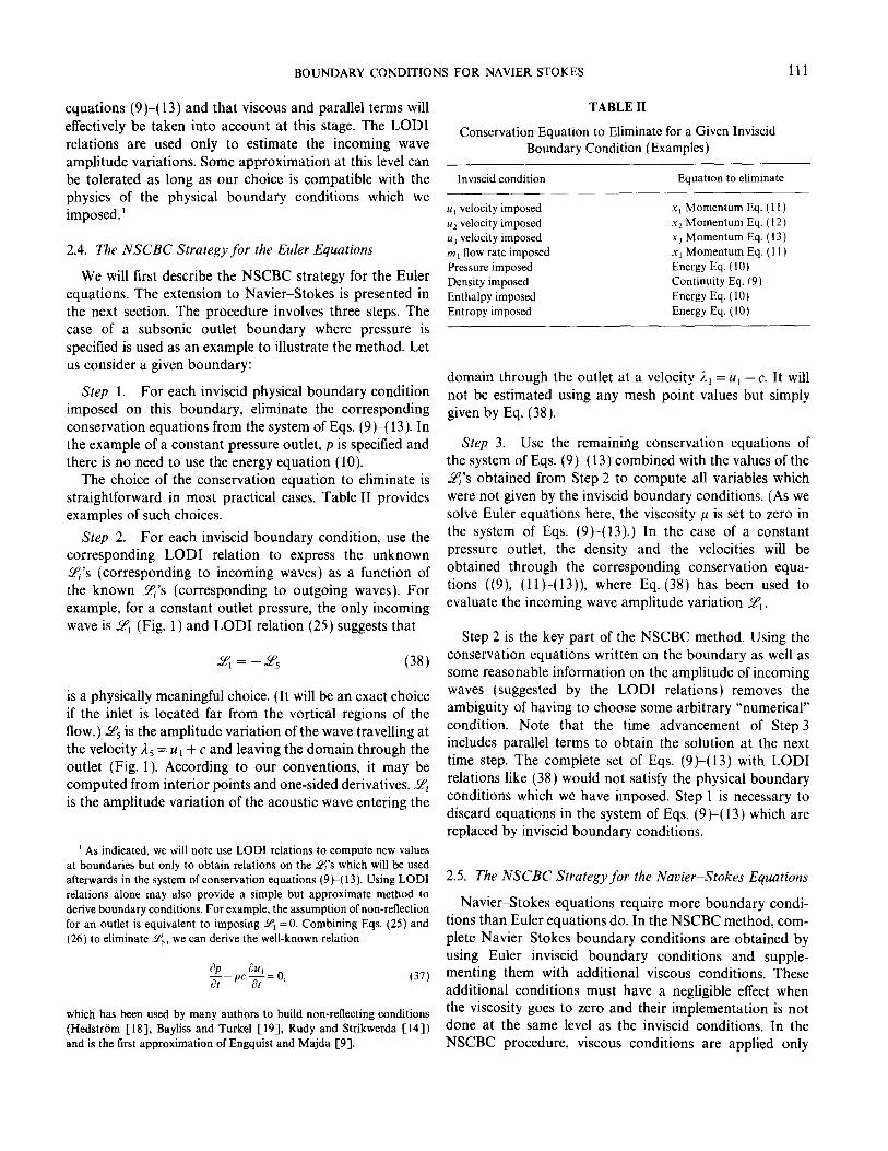
TABLE II

Conservation Equation to Eliminate for a Given Inviscid Boundary Condition (Examples)

Inviscid condition Equation to eliminate

u1 velocity imposed X, Momentum Eq. (11) u2 velocity imposed xz Momentum Eq. (12) u) velocity imposed x3 Momentum Eq. (13) m, flow rate imposed X, Momentum Eq. (1 I ) Pressure imposed Energy Eq. (10) Density imposed Continuity Eq. (9) Enthalpy imposed Energy Eq. (10) Entropy imposed Energy Eq. (10)

domain through the outlet at a velocity i, = u1 -c. It will not be estimated using any mesh point values but simply given by Eq. (38).

Step 3. Use the remaining conservation equations of the system of Eqs. (9)-( 13) combined with the values of the z’s obtained from Step 2 to compute all variables which were not given by the inviscid boundary conditions. (As we solve Euler equations here, the viscosity P is set to zero in the system of Eqs. (9~(13).) In the case of a constant pressure outlet, the density and the velocities will be obtained through the corresponding conservation equations ((9), (ll)-(13)), where Eq. (38) has been used to evaluate the incoming wave amplitude variation gl.

Step 2 is the key part of the NSCBC method. Using the conservation equations written on the boundary as well as some reasonable information on the amplitude of incoming waves (suggested by the LODI relations) removes the ambiguity of having to choose some arbitrary “numerical” condition. Note that the time advancement of Step 3 includes parallel terms to obtain the solution at the next time step. The complete set of Eqs. (9)-(13) with LODI relations like (38) would not satisfy the physical boundary conditions which we have imposed. Step 1 is necessary to discard equations in the system of Eqs. (9)-( 13) which are replaced by inviscid boundary conditions.

2.5. The NSCBC Strategy for the Navier-Stokes Equations

Navier-Stokes equations require more boundary conditions than Euler equations do. In the NSCBC method, complete Navier-Stokes boundary conditions are obtained by using Euler inviscid boundary conditions and supple- menting them with additional viscous conditions. These additional conditions must have a negligible effect when the viscosity goes to zero and their implementation is not done at the same level as the inviscid conditions. In the NSCBC procedure, viscous conditions are applied only


during Step 3 by specifying those viscous conditions are not strictly enforced by the NSCBC approach. They are only used to modify the conservation equations which are used in Step 3 to compute boundary variables which have not been specified by inviscid conditions. Steps 1 and 2 are the same for Euler and Navier-Stokes.

We have not indicated yet how to choose the viscous conditions. The compatibility of inviscid conditions with viscous conditions is not automatically ensured. Most Navier-Stokes codes actually use physical boundary conditions derived for the Euler equations. In particular, the number of physical conditions imposed on a given boundary is often chosen as if the flow were inviscid by arguing that the boundaries are far enough from the regions where viscous effects are important. As a consequence, only inviscid conditions are applied and no viscous conditions are introduced.

In the NSCBC method, the number and the choices of physical boundary conditions (inviscid and viscous) were guided using the theoretical studies of Strikwerda [32] and Oliger and Sundstrom [28]. However, the agreement between these studies and our own results is not complete as we will see later. Tables III and IV summarize the different physical conditions used in the NSCBC method for a three-dimensional flow and compare the number of these conditions with the number suggested by Strikwerda [32] and Oliger and Sundstrom [28] to ensure well-posedness. Table III corresponds to inlet and Table IV to walls and outlets. Only subsonic flows are considered here. The case of Euler equations is also displayed in the left column of each table to allow comparison with Navier-Stokes. The following facts are apparent:

l For inflow, we have listed four possibilities in Table III. The first column indicates whether a proof of well-posedness has been given for this set of conditions. The last column gives the theoretical number of conditions required for well-posedness (Strikwerda [ 321) and compares it with the number of conditions effectively used in the NSCBC method. For case SI 1, where ui, u2, u3, and Tare imposed, our method differs from the analysis of Strikwerda [32]. Only four conditions are used in the NSCBC method while Strikwerda claims that live conditions should be used. Indeed, imposing u1 , u2, us, and T is a special case because the only remaining unknown is the density p. p can be obtained through the continuity equation which does not involve any viscous term and does not require any additional condition, thereby leaving the total number of boundary conditions at four. In more general cases, however, we have found that live conditions are necessary as suggested by Strikwerda. For example, condition SI 2 (imposing u,, u2, uj, and p) is well posed for Euler equations (Oliger and Sundstrom [28]) and an additional viscous condition is provided in the NSCBC method for the

TABLE III

Physical Boundary Conditions for Three-Dimensional Flows for Euler and Navier-Stokes Equations

Elder N&e-Stokes

Inviscid Inviscid Viscous Number of BC conditions Number conditions + conditions used in NSCBC

4 + 0 =4?

Sl 1 u, imposed 4 u1 imposed Special case: No well-posed- u2 imposed u2 imposed Euler and NS

ness proof for u1 imposed u1 imposed need same Euler or NS T imposed T imposed conditions

4 + 1 =5

s12 Well-posed

for Euler. No proof for

NS [32]

u , imposed 4 ah u, imposed -=0 uz imposed u2 imposed ax,

u) imposed u) imposed p imposed p imposed

4 + 1 =5

Sl 3 u,-2c/(y-1) 4 u1 - W(Y - 1) 2=0 Didnot Well posed imposed imposed I work

for Euler uz imposed uz imposed (Unstable) and NS [32] u) imposed u1 imposed

s imposed s imposed

4 + 1 =5

s14 2!*=0 4 Ic;=o cp) Non reflecting. 9, = 0 Y,=O /

No proof for z4 = 0 Ya=O Euler and NS ‘$=o g=o

Note. Subsonic inflow. The boundary is located at x1 =0 (see Fig. 1). The theoretical number of boundary conditions required for well-posedness is 4 for Euler and 5 for Navier-Stokes (from [32]).

Navier-Stokes equations. This condition states that the normal stress is constant along the normal to the boundary and is close to the proposal of Dutt [29]. Imposing such viscous conditions on the viscous stresses makes more physical sense than trying to impose relations such as ~(&,/a~,) = 0 [28]. It is fair to say that only small effects are caused by these viscous conditions for inlets (this is not true for outlets). Most tests presented in this study have been performed with inflow conditions SI 1. Condition SI 2 gives similar results to SI 1.

l Condition SI 3 is the only one for which a well-posedness proof for Navier-Stokes has been given (Oliger and Sundstriim [28]). However, it is difficult to find a compatible soft condition for this case. ST 4 is the non-reflecting


TABLE IV

Boundary Conditions for Three-Dimensional Flows for Euler and Navier-Stokes Equations

Euler Navier Stokes

Inviscid Inviscid Viscous Number of BC conditions Number conditions

+ conditions NSCBC theory

1 + 3 =4

Subsonic Pat inlinity 1 P at infinity

non-reflecting is imposed is imposed

outflow

1 + 3 =4

Subsonic Pimposed 1 P imposed 2 = 0 ,

reflecting

Isothermal no-slip wall

4 + 0 =4

u, =o

UI = 0

u,=o T= cte

1 + 3 =4

Adiabatic u,=o I “, =o r,,=O r,,=O

slip wall 4, =o

Adiabatic

no-slip wall

3 + 1 =4

u, =o 41 =o u,=o u,=o

Note. Subsonic outflow and walls. The boundary is located at x, = L (see Fig. 1). The theoretical number of boundary conditions required for well-posedness is 1 for Euler and 4 for Navier-Stokes.

inlet treatment used for the NSCBC method. For the inviscid case, it only fixes relations on the wave amplitude variations. It is rather interesting to note that conditions SI 3 and SI 4 are equivalent for one-dimensional cases: they both express the conservation of entropy and the non-reflection of acoustic waves at the inlet section (this can be easily deduced from the LODI relations of Section 2.3). However, the principle of their implementation is quite different: SI 3 tries to enforce relations between primitive variables while SI 4 only fixes the waves amplitude variations through the boundary. For multidimensional flows, the implementation

of SI 4 using NSCBC is straightforward, but no satisfactory method could be found for SI 3.

l Outflow conditions are listed in Table IV. For non- reflecting subsonic outflow, one physical condition is needed for Euler equations but it has a specific form. This condition states that the pressure is imposed at infinity so that waves reflected from infinity towards the computation domain should have a zero amplitude. We will describe this case in more detail in Section 3.2. For the Navier-Stokes equations, three other conditions have to be added as suggested by Strikwerda [32]. We have tested many different combinations and the best choice appears to be quite close to the proposal of Dutt [29]: we impose that the tangential viscous stresses (ri2 and ri3 for a boundary at x1 = L) as well as the normal heat flux (ql = -1(8T/&,) through the boundary have zero spatial derivatives with respect to x1 (arIJ8x, = arlJ8x, = 0 and dq,/ax, = 0). These conditions relax smoothly to the inviscid conditions when the viscosity and the conductivity go to zero. They are implemented numerically by simple setting the derivatives along xl of z12, t13, and q, to zero on the boundary in the system of Eqs. (9)-(13). (This does not mean that the tangential viscous stresses or the normal heat flux are zero.)

As seen from Tables III and IV, the NSCBC method uses the right number of boundary conditions for Navier-Stokes equations for subsonic inflows, outflows, and walls (except for case SI 1) suggested by the studies of well-posedness [32]. This is also true for supersonic inflows where all variables are imposed in the NSCBC method and no viscous condition is used. This yields live boundary conditions as suggested in [32]. However, for supersonic ouflows, the NSCBC method uses three physical boundary conditions (no inviscid condition and three viscous conditions) so that it relaxes smoothly to the inviscid case when the viscosity goes to zero (for which no condition should be applied because the flow is supersonic) while Strikwerda [32] claims that four conditions should be applied. We have no explanation for this difference.

2.6. The Treatment of Edges and Corners

The treatment of corners in two-dimensional situations and of edges and corners in three-dimensional situations requires a simple extension of the NSCBC procedure. For edges, a second direction (for example, x2) has to be treated using characteristic relations. Terms of the type a/ax, on the left-hand side of the system of Eqs. (9)( 13) are replaced by characteristic waves amplitude variations estimated for the x2 direction. A second LODI system, relative to the x2 direction, has to be used to infer the values of the different waves along x2. The viscous terms are simply corrected for viscous conditions and added as for the usual boundaries. The extension to corners in three dimensions is straight-


forward although relatively cumbersome to implement. Our own experience indicates that these edge and corner treatments are necessary when a centered interior scheme (with low dissipation) is used.

Like any other formulation, the NSCBC approach for edges and corners requires some compatibility conditions to be satisfied at these locations. For example, the corner between a no-slip wall and a constant pressure outlet should have a variable pressure (which is the only floating variable on a no-slip wall). This is not compatible with the outlet specification where the pressure is imposed. Imposing the pressure as well as all other variables at the corner seems a possible solution but it does not work. A solution (used in Section 6) is to obtain the pressure at the corner through a NSCBC corner treatment. At steady state, this pressure reaches the outlet pressure, but during the time dependent evolution, it allows smooth transients. A general definition of possible combinations of boundary conditions for edges and corners remains to be given and appears to be even more difficult than the usual studies of well-posedness.

3. EXAMPLES OF IMPLEMENTATION

Although all recent methods developed for Euler boundary conditions emphasize the importance of characteristic lines, many differences appear in the practical implementation of the characteristic relations and the choice of soft conditions, especially in multi-dimensional flows. The situation is even more complex for Navier- Stokes cases. It is therefore necessary to go now into more detail by presenting the practical implementation of the NSCBC method in the following typical situations:

3.1. A subsonic inflow 3.2. A subsonic non-reflecting outflow 3.3. A subsonic reflecting outflow 3.4. An isothermal no-slip wall 3.5. An adiabatic slip wall 3.6. An adiabatic no-slip wall.

The geometry is given in Fig. 1 where the section xi = 0 corresponds to the inlet and xi = L to the outlet boundaries. The problem of non-reflecting boundaries will be given more attention as it raises certain additional difficulties. Supersonic cases will not be discussed here because they are usually simpler than subsonic cases.

3.1. A Subsonic Inflow

Many “physical” boundary conditions exist for subsonic inflow conditions. We have chosen to describe a case where all components of velocity u,, u2, and u3 as well as the temperature T are imposed (Case SI 1 in Table IV). These

quantities can change with time and are functions of the spatial location in the inlet plane x, = 0:

u,(O, x2, x3> t) = w,, x3, f) u,(O, x2, x3,1) = T/(x,, x3, t) u,(O, x2, x3, t) = W(x,, x3, f) T(O, x2, x3, t) = P2, x3, t).

This case is typical of direct simulations of turbulent flows where we wish to control the inlet shear and introduce flow perturbations. For a subsonic three-dimensional flow, four characteristic waves are entering the domain (Fig. I), Y2, Y3, PA, and Y5, while one of them (Pi) is leaving the domain at the speed 2, = ui - c. Therefore, the density p (or the pressure p) has to be determined by the flow itself. We have four physical boundary conditions (for ui , u2, u3, and T) and one soft boundary condition (for p). No viscous relation is needed for this case. To advance the solution in time on the boundary, we need to determine the amplitudes z of the different waves crossing the boundary. Only one of these waves (3;) may be computed from interior points. The others are given by the NSCBC procedure, as follows:

Step 1. The inlet velocities U, , u2, and u3 are imposed, therefore Eqs. (11) (12), and (13) are not needed. The inlet temperature is imposed and the energy equation (10) is not needed any more.

Step 2. As the inlet velocity ui is imposed, the LODI relation (26) suggests the following expression for Pi :

As the inlet temperature is imposed, the LODI relation (29) gives an estimate of the entropy wave amplitude Z2 :

LODI relations (27) and (28) show that T3 = -dV/dt and Y4 = - d W/dt.

Step 3. The density p can now Eq. (91,

be obtained by using

dP %+d, +& (Pu2 )=O, (9) 2

where d, is given by Eq. (14):


LZ’~ is computed from interior points using Eq. (19). -!Z$ and L?‘~ have been determined at Step 2. In this case, LZ~ and LZY are not needed.

3.2. A Subsonic Non-reflecting Outflow

Using non-reflecting boundary conditions for Navier- Stokes equations is very appealing but requires some caution. The first point to emphasize is that building a perfectly non-reflecting condition might not lead to a well- posed problem. Suppose that we want to compute a free shear layer by using the inlet boundary conditions described in the previous section, i.e., by imposing the inlet velocities and the temperature. If we build “perfectly non-reflecting” boundary conditions for the three other sides of our domain, we should wonder how the flow will determine what the mean pressure will be. Physically, this information is conveyed by waves reflecting on regions far from the computation domain where some static pressure pm is specified and propagating back from the outside of the domain to the inside through the boundaries. With perfect boundary conditions this information will never be fed back into the computation and the problem might be ill-posed. This problem has been recognized by some authors and solutions have been proposed (Rudy and Strikwerda [ 14, 151, Keller and Givoli [34], Hagstrom and Hariharan [36]). Corrections may be added to the treatment of boundary conditions to make them only partially non-reflecting. This is the principle of the treatment proposed in the NSCBC approach.

domain while one of them LZ’i is entering it at the speed A1 = ui - c. Specifying one inviscid boundary condition for the primitive variables would generate reflected waves. For example, imposing the static pressure at the outlet p = pm leads to a well-posed problem (Oliger and Sundstrom [ 28 ] ) which will, however, create acoustic wave reflections. Avoiding reflections apparently forces us to use only “soft” boundary conditions. But as indicated above, we want to add some physical information on the mean static pressure px to our set of boundary conditions so that the problem remains well-posed. After the waves have left the computational domain, we except the pressure at every point of the outlet to be close to pm. An appealing but expensive way to do that would be to match the solution on the boundary with some analytical solution between the boundary and infinity. We have chosen a simpler method requiring only a small modification to the basic NSCBC procedure:

Step 1. We have one special physical boundary condition: the pressure at infinity is imposed. This condition does not fix any of the dependent variables on the boundary and we keep all conservation equations in the system of Eqs. (9)-( 13).

Step 2. The condition of constant pressure at infinity is now used to obtain the amplitude variation of the ingoing wave 2, : if the outlet pressure is not close to pa, reflected waves will enter the domain through the outlet to bring the mean pressure back to a value close to pm. A simple way to ensure well-posedness is to set

It is also important to realize that one-dimensional and multi-dimensional flows are quite different as far as non- reflecting boundary conditions are concerned. Extending boundary conditions derived and tested in one-dimensional situations to multi-dimensional cases requires substantial modifications to take into account the transverse terms at the boundaries. Different tests (not presented here) indicate that perfectly non-reflecting boundary conditions for Euler equations may provide well-posed formulations in one- dimensional cases and ill-posed formulations in most two- dimensional situations. This fact has been observed also by Bayliss and Turkel [ 191. The NSCBC method allows a non-reflecting treatment for boundaries which is exact for one-dimensional problems and remains well-posed for multi-dimensional problems. However, in the multi-dimensional case, the non-reflecting treatment is not exact in the sense that waves which do not reach the boundary at a normal incidence are not perfectly transmitted. For these waves, the NSCBC treatment leads to small levels of reflection but still prevents numerical oscillations and ensures well-posedness.

%=K(P-P,), (40)

where K is a constant: K= a( 1 -4’) c/L. & is the maximum Mach number in the flow, L is a characteristic size of the domain, and (T is a constant. The form of the constant K is the one proposed by Rudy and Strikwerda [14] who derived a similar correction but applied it only in the energy equation (see Section 4.1). When c = 0, Eq. (40) sets the amplitude of reflected waves to 0. This is the method used by Thompson [ 1 ] and we will call it “perfectly non-reflecting.”

Some problems are simple enough to allow the determination (through asymptotic methods, for example) of an exact value LYqXac’ of 2,. Then Eq. (40) should be written:

9, = K(p - p,) + ,qXact.

The second term will ensure an accurate matching of derivatives between both sides of the boundary while the first term will keep the mean values around pm. In practice, we have found that in most problems, Eq. (40) can be used directly without an additional term.

Considering a subsonic outlet where we want to imple- If we are considering a viscous flow, the viscous condi- ment non-reflecting boundary conditions (Fig. l), we see tions (Table IV) require that the tangential stresses r12 and that four characteristic waves, &, Y;, Tdq, and 6ps leave the z 13 and the normal heat flux q 1 have zero spatial derivatives


along xi. Let us recall that the conditions on the tangential stresses and the heat flux are implemented directly in the system of Eqs. (9)-j 13) by setting their derivatives along the normal to the boundary to zero.

Step 3. All the z’s with i # 1 may be estimated from interior points. Ti is given by Eq. (40) and the system of Eqs. (9)-(13) may be used to advance the solution in time on the boundary.

3.3. A Subsonic Rejlecting Outflow

For certain cases, for example, to study coupling mechanisms between longitudinal acoustic waves and vortex shedding in a shear layer, enforcing an exact reflection of waves at the boundary may be of interest. Imposing an inviscid condition at an outlet (constant pressure or constant velocity, for example) will induce wave reflections. This is done here for the case of an imposed outlet static pressure (p(L, x2, x3, t) = P(x,, xj, t)):

Step 1. As the pressure at the outlet is imposed, Eq. (10) is not needed any more.

Step 2. LODI relation (25) suggests that the amplitude of the reflected wave should be

According to Table IV, we also impose constant tangential stresses and a constant normal heat flux through the boundary if we solve the Navier-Stokes equations.

Step 3. All the g’s with i# 1 may be estimated from interior points. Y1 is then obtained through the relation given in Step 2 and Eqs. (9), (1 1 )-( 13) are used to obtain p, Ul, u23 and u3 on the boundary at the next time step.

3.4. An Isothermal No-Slip Wall

At an isothermal no-slip wall, all velocity components vanish and the temperature is an imposed function of time and space location. We have four inviscid boundary conditions for this case (u,(L, x2, -x3, t) = u,(L, x2, xg, t) = u,(L, x2, x3, t) = 0 and T(L, x2, xj, t) = 7(x,, x3, t)) and no viscous relation:

Step 1. As velocities u,, us, and u3 are fixed, Eq. (1 1 ), (12), and (13) are not needed. As the temperature is imposed, the energy equation (10) is also discarded.

Step 2. LODI relation (26) suggests that the amplitude of the reflected wave should be 6pl= Zs. The characteristic amplitudes Z2, g3, and YZ are zero because the normal velocity u1 is zero.

Step 3. Computing the value of gs from interior points, we set 9, = =!& and compute the density p from integration of Eq. (9).

Note that moving or vibrating no-slip walls may be implemented by simply keeping time dependent velocities in the LODI relations (26)-(28).

3.5. An Adiabatic Slip Wall

Slip walls are useful boundary conditions in some computations. They are characterized by only one inviscid condition: the normal velocity at the wall is zero (u,(L, x2, x3, t) = 0). The viscous relations (Table IV) correspond to zero tangential stresses and a zero heat flux through the wall. As the normal velocity is zero, the amplitudes gZ, -rZ;, and Yd are zero (from Eqs. (20)-(22)). One wave JX~ is leaving the computation domain through the wall while a reflected wave 2, is entering the domain:

Step 1. The velocity u1 normal to the wall is zero and Eq. (11) is not needed.

Step 2. LODI relation (26) suggests that the amplitude of the reflected wave should be: Z1 = Y5.

Step 3. zZ~ is computed from interior points and Y1 is set to gs. The derivatives along x, of the tangential viscous stresses ri2, r13 and of the normal heat flux q1 at the wall are computed using the viscous conditions at the wall: q, = 0, ri2 = rr3 = 0. Remaining variables (p, u2, uj, and T) are obtained by integration of Eqs. (9k(lO) and (12)-( 13).

3.6. An Adiabatic No-Slip Wall

At an adiabatic no-slip wall, all velocity components vanish and the heat flux is zero. We have only three inviscid physical conditions (ur(L, x2, x3, t) = u,(L, x2, x3, t) = 0). They are complemented by one viscous conditions: the heat flux through the wall q, is zero:

Step 1. As velocities ui , u2, and u3 are fixed, Eqs. ( 1 1 ), ( 12), and (13) are not needed.

Step 2. LODI relations (26), (27), and (28) show that Yi = Z5 and Y3 = Yd = 0. The characteristic amplitudes Y;, &, and pd are zero because the normal velocity is zero.

Step 3. Computing the value of gs from interior points, we set Z1 to Y; in the system of Eqs. (9)-(13). Viscous conditions are implemented as in the previous section: the condition q1 = 0 is used during the estimation of 8q1/ax1 at the wall. The density is then obtained from integration of Eq. (9), the total energy from Eq. (10).

4. APPLICATIONS TO STEADY FLOWS

All tests of the NSCBC method are described in Poinsot and Lele [ 381 and are summarized in Table V. We will only give some examples here: a ducted shear layer (Section 4), a vortex leaving the computation domain through a non- reflecting outlet (Section 5), and a Poiseuille flow (Sec-


TABLE V

The Test Configurations for the NSCBC Method

TYPO and Grid

Schematac Specdicatlons for boundary conditions

2D Steady

state

41 x 41

Lateral slip walls Imposed mlei veloc111es and temperature. Reflec+ng or non refletilng outlet.

Non reflectmg baundanes on sides and

2D Steady

state 121 x81

No-slip lateral walls. Non rellectmg outlet. Imposed inlet velocities and temperature (arbitrary profiles)

tion 6). Cases described in this paper are two-dimensional. Additional tests for non-reacting free shear layers, steady, and unsteady reacting flows and acoustic wave transmission through non-reflecting boundaries may be found in [38].

The first case is a steady laminar shear layer. Although all computations presented are time-dependent, steady-state solutions are used here as a test case for the consistency of the method. This test is a difficult one for many codes because it reveals the weaknesses of the boundary condition treatments. Buell and Huerre [24] show, for example, that direct simulation codes for incompressible flows may generate self-sustained oscillations in shear layers because of a numerical coupling mechanism between the outlet and the inlet of the domain. Vortices leaving the computation domain introduce inlet perturbations which create other vortices. This feedback may force the shear layer to oscillate in a self sustained mode which is non-physical. We will show that similar coupling mechanisms can be due to high frequency numerical instabilities generated by boundary reflections and interactions with inlet conditions, as shown by Vichnevetsky and Pariser [30] and Vichnevetsky [313.

As we are interested first in the stability and convergence of the method used to treat the boundaries, we will consider only domains with small streamwise dimensions in order to provide fast convergence to steady state. Our first goal is to demonstrate the influence of the boundary conditions on

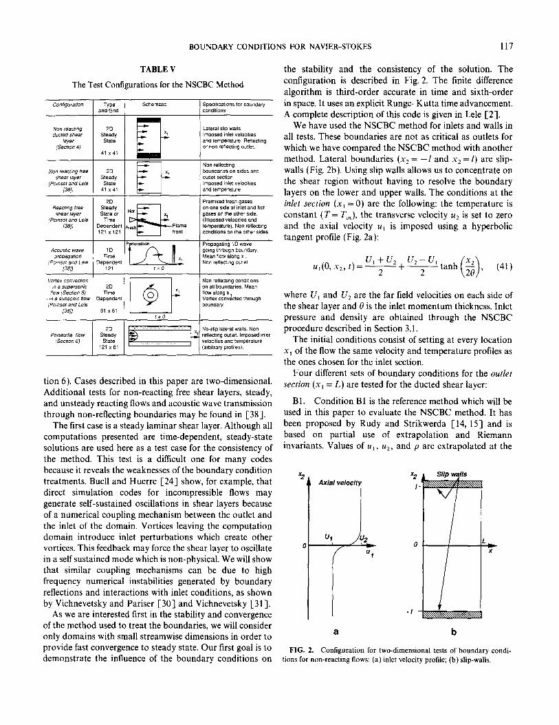
the stability and the consistency of the solution. The configuration is described in Fig. 2. The finite difference algorithm is third-order accurate in time and sixth-order in space. It uses an explicit Runge-Kutta time advancement. A complete description of this code is given in Lele [2].

We have used the NSCBC method for inlets and walls in all tests. These boundaries are not as critical as outlets for which we have compared the NSCBC method with another method. Lateral boundaries (x2 = -1 and x2 = E) are slip- walls (Fig. 2b). Using slip walls allows us to concentrate on the shear region without having to resolve the boundary layers on the lower and upper walls. The conditions at the inlet section (x, = 0) are the following: the temperature is constant (T= Ti”), the transverse velocity u2 is set to zero and the axial velocity u, is imposed using a hyperbolic tangent profile (Fig. 2a):

u1(0,x2, l)=---- ~ u,+u, Udbtanh 2 2 + 2 ( > 29 ’ (41)

where U, and U2 are the far field velocities on each side of the shear layer and 0 is the inlet momentum thickness. Inlet pressure and density are obtained through the NSCBC procedure described in Section 3.1.

The initial conditions consist of setting at every location x1 of the flow the same velocity and temperature profiles as the ones chosen for the inlet section.

Four different sets of boundary conditions for the outlet section (x1 = L) are tested for the ducted shear layer:

Bl. Condition Bl is the reference method which will be used in this paper to evaluate the NSCBC method. It has been proposed by Rudy and Strikwerda [ 14, 151 and is based on partial use of extrapolation and Riemann invariants. Values of u,, u2, and p are extrapolated at the

Axial velocity

a b

FIG. 2. Configuration for two-dimensional tests of boundary conditions for non-reacting flows: (a) inlet velocity profile; (b) slip-walls.


outlet (zeroth-order extrapolation is used). The pressure is obtained from the non-reflecting condition:

where the term K(p - p,) is similar to the correction term introduced in the NSCBC formulation in Section 3.2: K= a’( 1 - A’) c/L. By studying analytically the behavior of Eq. (42) for a linearized constant coefficient one-dimensional system of equations, Rudy and Strikwerda [14] derived an optimal value for 0’ around 0.27. However, their tests [14, 151 show that a value of 0.58 provides the best results in practice. The main differences between this approach and the NSCBC method are the use of extrapolation and the introduction of a corrective term K(p - p,) in the energy equation for the reference method while the NSCBC method does not use any extrapolation and introduces a correction on the incoming wave amplitude ~3~ only (Eq. 40).

B2. Condition B2 is obtained by the NSCBC formulation with cr = 0. It corresponds to perfectly non-reflecting boundary conditions (Section 3.2). No extrapolation is involved at any stage.

B3. Formulation B3 is the corrected non-reflecting NSCBC formulation with c = 0.25 (Section 3.2).

B4. Condition B4 corresponds to a reflecting outlet maintained at a constant static pressurep, and treated with a NSCBC procedure described in Section 3.3.

Conditions B2 to B4 are all obtained by NSCBC. Condi- tion Bl may be viewed as the prototype of a method which has been used by many other authors to treat subsonic outflow boundaries. Grinstein et al. [26] use zeroth- and lirst- order extrapolations respectively for density and velocity and apply a relaxation procedure for the pressure which is similar to condition Bl. First-order extrapolations for the density and the velocity with fixed pressure are used by Yee [17]. Jameson and Baker [27] extrapolate tangential velocity and entropy and obtain the longitudinal velocity and the pressure through Riemann invariants. All these methods use extrapolation for two or more variables at the outlet. Although condition Bl was apparently designed to compute steady state flows, it appears that it has been used in many unsteady cases because of its simplicity. As suggested by one of the reviewers, more recent methods may have been used to evaluate the performances of the NSCBC technique. However, condition Bl is simple, well-known, and widely used. It is used here only to provide a reference to which the NSCBC may be compared. We reckon that other recent techniques may also provide excellent results and should be compared to the NSCBC method. This has been left for further studies.

The parameters for the computation are the following (velocities are normalized by the sound speed c and lengths by the half width of the duct I):

u,/c = 0.9, U,/c = 0.81, Re = UZ lf v = 2000,

8/l = 0.025, L/l= 1.

The maximum Mach number of this flow is: .& = U,/c = 0.9. A coarse computation grid (41 by 41) is used to allow many test runs. The grid resolution does not change the intrinsic performance of the boundary conditions.

Figures 3 to 6 display the time variations of the inlet and outlet flow rates (obtained by simple integration along x2 of the axial flow rate m, at the inlet and outlet sections). The flow rates are normalized by the initial inlet density, the sound speed, and the duct half width. A reduced time of 50 allows more than 40 travels at the mean convection speed ( U1 + UJ2c = 0.85 for a particle between the inlet and the outlet of the computation domain and is considered long enough for the flow to reach steady state.

Figure 3 shows results obtained using boundary conditions Bl. The coefficient 6’ is equal to 0.58 as suggested by Rudy and Strikwerda [ 141. This condition allows waves to be transmitted at the outlet and seems to work reasonably well until a reduced time of 30. If the computation is con- tinued, no steady state is obtained. The inlet and outlet flow rates oscillate. The amplitude of these oscillations is a function of the initial condition and of the waves generated at the beginning of the computation. It is interesting to note that Rudy and Strikwerda did not encounter such problems when they used this formulation to compute a boundary layer over a flat plate [lS]. This might be due to the fact that these authors were using a MacCormack scheme which introduces artificial dissipation and allows the code to damp the oscillations appearing on Fig. 3. When a non-dissipative code such as the present one is used, the errors due to the extrapolation procedure at the outlet boundary are never damped. We will come back to this problem in Section 5.

- I tntet --____ : out/et

0 25 Reduced t/me (c t / LI !

FIG. 3. Time variations of the inlet and outlet flow rates for a non- reacting ducted shear layer. Boundary conditions Bl (reference method with u’ = 0.58).


‘6 25 Reduced t/me (c t / L) 50

FIG. 4. Time variations of the inlet and outlet flow rates for a non- reacting ducted shear layer. Boundary conditions B2 (NSCBC perfectly non-reflecting method).

Figure 4 presents the results obtained with the perfectly non-reflecting condition B2. In this case, waves are eliminated rapidly (Fig. 4) but the solution does not converge. Although the pressure and temperature fields are smooth and correspond to reasonable results, the mean pressure in the domain keeps decreasing linearly. The inlet and outlet flow rates which are directly functions of the mean pressure decrease, too, and no steady state can be reached. The Navier-Stokes equations with perfectly non- reflecting conditions appear to be ill-posed in this case.

Figure 5 displays the results corresponding to the corrected non-reflecting condition B3 with a parameter cr =0.25. In this case, waves are eliminated and the solution converges to a steady state after a reduced time (et/l) = 25. The mean pressure reaches a constant value and the inlet and outlet flow rates become equal.

The influence of the constant (T is weak. We have used r~ = 0.25 in most NSCBC tests. Values of this parameter equal to 0.1, 0.25, and 0.4 were tested: 0 = 0.1 produced a drifting solution similar to the one obtained for 0 = 0 (Fig. 4) while the two other choices yielded satisfactory and almost identical results. Increasing CJ beyond certain limits (here (T N 0.7) leads to large flow oscillations. Note that the optimum value of 0 is close to the optimal value of 0’

i;k 1 b is

* Reduced r/me (c t / L) 50

FIG. 5. Time variations of the inlet and outlet flow rates for a non-reacting ducted shear layer. Boundary conditions B3 (NSCBC non- reflecting method with e = 0.25).

* a 25 Reduced t/me c t I L 50

FIG. 6. Time variations of the inlet and outlet flow rates for a non- reacting ducted shear layer. Boundary conditions B4 (NSCBC reflecting method with a constant outlet pressure).

(Eq. 42) derived analytically by Rudy and Strikwerda [ 141. Although 0 = 0.25 provided good results for all the tests described in Poinsot and Lele [38], (r might have to be adjusted for other specific configurations or other numerical methods.

Finally, the behavior of the solution for a reflecting outlet (condition B4) is illustrated on Fig. 6. In this case, no steady state is reached because the first longitudinal acoustic mode of the system cannot leave the domain. This mode is damped only by viscous dissipation and would still be present after a longer time. Its period t, can be easily evaluated using the duct length L/l = 1 and the mean Mach number & = 0.85 by:

(ct,/L) = & ‘v 14. (43)

Figures 3 to 6 show that the existence of a steady state solution is a strong function of the boundary conditions used for the outlet section. Although the oscillation displayed in Fig. 3 for the reference method or the drift in the mean values encountered for the perfectly non-reflecting NSCBC method in Fig. 4 are small, these effects are a clear manifestation of the inadequacy of these treatments. Furthermore, even a correct treatment of the outflow condition like the case of condition B4 in Fig. 6 may not lead to a steady state if reflections are allowed on the boundary. Although reflections may be of interest in certain cases, they create an additional coupling between acoustic waves and the hydrodynamic field. Suppressing this coupling in direct simulations is clearly useful in many cases and this may be achieved by using the non-reflecting NSCBC method B3.

5. APPLICATIONS TO UNSTEADY FLOWS

We have demonstrated the ability of the NSCBC procedure to perform steady state computations. The present example is devoted to truly unsteady flows. The goal here


is to characterize the performance of outlet boundary treatments for time-dependent flows.

Let us first describe important results on boundary conditions for unsteady flows which have been obtained by Vichnevetsky and Bowles [33] in the case of the advection equation:

(44)

In this situation, when an unsteady perturbation reaches a boundary (Fig. 7a), two types of waves are present near the boundary: physical waves called “p” waves by Vichnevetsky [3 1 ] and numerical waves called “q” waves. The physical waves have long wavelengths and correspond to the incident perturbation crossing the boundary. They are the physically meaningful part of the solution. The numerical waves have short wavelengths (smaller than four times the mesh size for a centered second-order scheme [ 333 ) and are spurious waves generated by the discrete treatment of the boundary conditions. Once “q” waves are generated, their behavior depends on their group velocity ug; ug is a function of the scheme spatial differencing method. It is proportional to U and may be conveniently characterized by k, = u,/U. The ratio k, is generally negative so that “q” waves travel upstream and are called reflected numerical waves. For classical Pade schemes [33], (k,( increases with the scheme

incident physical wave

1 Incident Dhvsic8l w8ve htach=u/ccl

kpeed = u ; C.-amplitude I

= Ah

b

Reflected numerical wave I I Speed = ug c 0 , amplitude = A,

FIG. 7. Numerical and physical reflected waves at an outlet boundary: (a) the advection equation; (b) the Euler equations.

order. It also increases with the oscillation frequency and reaches a maximum for “saw-tooth” oscillations which have a wavelength equal to 2 dx, . Second-order central differences will lead to a maximum group velocity U, given by k, = u,/U= - 1 [33]. The classical fourth-order Pade scheme leads to k, = - 3 while the sixth-order Pade scheme used in this paper leads to k, = - 1313. When “q” waves reach another boundary (an inlet boundary in the case of Fig. 7a, for example), they are reflected in the form of a physical wave which is convected downstream again (Vichnevetsky and Pariser [30]). As a result, “q” waves create a feedback between inlet and outlet which is entirely numerical.

Although the results of Vichnevetsky and Bowles [33] have been obtained for the advection equation, they can be extended to the linearized Euler equations (acoustic theory). There is, however, an additional complexity for Euler equations: acoustic waves can be reflected by boundaries into physical waves. In a subsonic flow, an acoustic wave propagating at the speed u + c and reaching a reflecting outlet boundary (where the outlet pressure is imposed, for example) will generate two reflected waves (Fig. 7b): the first will be a physical wave of type “p” propagating upstream at the speed u-c. This wave is the physically meaningful part of the reflected wave. A “q” wave will also be reflected and propagate upstream at the speed ug = k,(u + c). In a supersonic flow, no reflected “p” wave will be created, but the “q” wave will still be generated. It will travel upstream at ug, reach the inlet of the computational domain, and induce non-physical perturbations. Therefore using supersonic outlets [6, 71 cannot be viewed as a general simple solution to treat outflow boundary conditions; physical “p” waves do not travel upstream in a supersonic flow but numerical “q” waves do.

Now, the strength of this numerical feedback is determined by the amplitude of the reflected numerical “q” wave. This amplitude is mainly fixed by the quality of the outflow boundary condition treatment. (Approximate treatments of boundary conditions lead to large numerical reflected waves.) Note that two reflection coefficients must be used to characterize a given boundary condition treatment: the reflection coefficient of physical waves A,/A , and the reflection coefficient of numerical waves A,,/A 1 (A, is the amplitude of the incident physical wave). In all cases, an adequate boundary condition treatment requires the amplitude of the numerical reflected waves to be small Ay/A, 4 1. An adequate non-reflecting boundary condition treatment also requires small physical reflected waves (APIA 14 1).

The quality of a non-reflecting boundary condition treatment may be studied by considering simple waves leaving the computation domain through an outlet boundary. The transmission of one-dimensional acoustic waves through a non-reflecting boundary is a well-known test and the NSCBC method allows complete transmission of incident


acoustic waves with very small levels of physical and numerical reflections (Poinsot and Lele [38]). On a grid using 121 points, typical reflection coefficients for one- dimensional Gaussian waves with a 15 points half-width are A,,A, N 10e4 and A,/A, < 1O-6 (these values correspond to small amplitude acoustic waves reaching the boundary at normal incidence). We have chosen to present here a two- dimensional case which is more typical of direct simulations of turbulent flows: a vortex propagating through a non- reflecting boundary.

The configuration corresponds to a vortex superimposed on a plug flow (velocity u,,) and convected downstream (Fig. 8). The mean flow is supersonic (uO/c = 1.1). Super- sonic mean flow was chosen to show that the numerical coupling described in Fig. 7 can occur in supersonic cases. (The case of a subsonic mean flow is presented in Poinsot and Lele [38] and leads to similar results.) The lateral boundaries are non-reflecting. The velocity field of the vortex is initialized at t = 0 using the stream function $ for an incompressible non-viscous vortex in cylindrical coordinates (the coordinate origin is located on the vortex center):

/ !!L\

(::)=(;)+l,P( ;; )> \-GJ (45)

+=Cexp( -y).

C determines the vortex strength. R,. is the vortex radius. This vortex has a central core of vorticity with the same sign as C surrounded by a region of vorticity of the opposite sign. This structure is useful for numerical simulations because the total circulation is zero. No correction is required initially for the boundary values (Rutland and Ferziger L-251).

uniform supersonic Inlet flow at spwd u.

Non r.sfktlng laterat waJ/s

I \

Non reflecting outlet section

Vorlex convected

FIG. 8. Configuration for two-dimensional tests of non-reflecting outlet boundary conditions: vortex propagating through a supersonic outlet.

The pressure field is initialized as:

p-py=P$exp( -$$).

The mean flow characteristics used for this case are

Jzz=uu,/c= 1.1, Re = uOl/v = 10,000,

L/l = 2.

(46)

(47)

The vortex is initially located in the center of the domain (x, = I, x2 = 0) and is defined by

RJI = 0.15, C/( cl) = - 0.0005. (48)

Inlet and lateral boundaries were treated using the perfectly non-reflecting NSCBC procedure. Two sets of boundary conditions were used for the outlet:

Bl. Reference method with c’= 0.58 (Rudy and Strikwerda [ 14, 151).

B3. Non-reflecting NSCBC conditions with d = 0.25.

It is necessary to recall here that condition Bl is a crude method based on extrapolations near boundaries. There- fore, it is expected to perform poorly in transient situations. It is shown here only because of its simplicity and because it is still used by some authors. As such, it provides a correct reference method. Figure 9a shows the initial vorticity and longitudinal velocity fields computed using conditions Bl. (The vorticity is normalized by c/l.) Dashed lines correspond to negative values of the isolines while solid lines indicate positive values. The longitudinal velocity u1 is plotted as (u, - u,)/u, so that dashed lines correspond to flow locally slower than the mean speed u0 while solid lines reveal flow faster than uO. In Fig. 9, the vortex is turning counterclockwise. The central core of negative vorticity (Fig. 9a) is surrounded by a ring of positive vorticity. This structure is characteristic of the stream function defined by Eq. (45). The vortex is convected downstream at the mean flow speed uO/c = 1.1. The maximum speed induced initially by the vortex is 0.0018~~.

After a reduced time (et/r) N 1, the vortex leaves the computation domain (Fig. 9b). Condition Bl does not allow the vortex to leave the domain without creating instability. The initial structure of the vorticity field is modified. A careful examination of the vorticity profiles indicates that the vorticity is not continuous at the outlet. The longitudinal velocity contour also exhibits numerical instabilities (“q” waves) which are characteristic of an incompatibility between the vertical flow and the boundary conditions treatment. The second effect of these instabilities is similar to the one presented in Fig. 7: the numerical waves


v I FIG. 9. Vorticity and longitudinal velocity fields at three instants

(cr/l) = 0, 1, and 2 for a vortex leaving the computation domain. Boundary conditions Bl (reference method with (r’ = 0.58).

propagate upstream at high speed, are reflected on the upstream section, and induce inlet perturbations (Fig. 9b) and, later, the formation of a new vortex at the inlet (Fig. SC). At (ct//) = 2, this new structure is near the center of the computation domain and convected downstream. It is turning clockwise and its maximum vorticity is around 0.15 times the initial maximum vorticity in Fig. 9a. Although the flow is supersonic, condition Bl creates a numerical feedback between inlet and outlet. This makes the method unacceptable for direct simulation.

Figure 10 displays results obtained with the non- reflecting NSCBC procedure B3. The initial condition (Fig. 10a) is the same as in Fig. 9a. When the vortex leaves the domain at a reduced time (cl/l) = 1, the vorticity field is preserved (Fig. lob) and the longitudinal velocity field is smooth. The amplitude of the reflected numerical waves is low and no noticeable perturbation appears on the inlet section. At later times ((et/Z) = 2), the original vortex has disappeared and the only perturbation generated at the inlet corresponds to a vortex with a maximum vorticity which is 1O-4 times the initial maximum vorticity.

It is worth indicating that the perfectly non-reflecting boundary conditions B2 (0 = 0) produce exactly the same

results as the B3 procedure: the vortex leaves the domain smoothly and there is no drift of the mean values afterwards. The perfectly non-reflecting boundary conditions B2 of the NSCBC method lead to well-posed problems in one-dimensional situations (Poinsot and Lele [38]) and also in two- dimensional cases where the mean flow does not exhibit transverse gradients near the boundary. The latter flows are, in fact, almost one-dimensional even if their perturbations are two-dimensional.

Finally, Fig. 11 displays the time variations of the maximum vorticity intensity and of the total absolute vorticity for the two boundary conditions Bl and B3. In both cases the maximum vorticity decreases slowly at first because of viscous effects between reduced times 0 and 1 and more rapidly afterwards when the vortex leaves the domain. The maximum and the total vorticity go exactly to zero for the NSCBC calculation after the vortex has left the domain (Fig. 1 1 ), but not for the reference method. Furthermore, condition Bl does not allow the vorticity to decrease monotonically (Fig. 1 la). During the convection of the structure through the boundary, the maximum vorticity is increased which is a non-physical result. On the contrary, condition B3 gives a monotonic decrease of the maximum

h&X: 1.88-3

FIG. 10. Vorticity and longitudinal velocity fields at three instants (cr/l) = 0, 1, and 2 for a vortex leaving the computation domain. Boundary conditions B3 (NSCBC non-reflecting method with IJ = 0.25).

BOUNDARY CONDITIONS FOR NAMER-STOKES 123

a .06

NSCBC method 83

4. Reduced time

b ,005

,004

,003

,002

,001

,000 u. 1. 2.

Reduced time 3. 4.

FIG. 11. Time variations of maximum vorticity (a) and total absolute vorticity (b) for a vortex leaving the computation domain. Comparison between the reference method Bl (thin line) and the NSCBC method B3 (thick line).

vorticity. (The two-step variation of the maximum vorticity for boundary conditions B3 corresponds to the passage of the central core followed by the ring of vorticity of opposite sign. )

This last test confirms the importance of the downstream boundary condition on the global result. Let us note that the mechanism evidenced here has no relation to the compressible character of the flow. Similar results are obtained by Vichnevestky and Pariser [30] for the simple advection equation where no physical information can travel upstream and by Buell and Huerre [24] for an incompressible flow (although Buell’s incompressible formulation introduces additional complexity through the implicit determination of pressure). It is purely numerical and entirely a function of the boundary condition treatment.

6. APPLICATIONS TO LOW REYNOLDS NUMBER FLOWS: THE POISEUILLE FLOW

The last example concerns a very low Reynolds number where u, is the maximum velocity on the axis: U, = flow with isothermal no-slip walls: the Poiseuille flow. This - ( i/2p)(aff==yX,) 12.

is a difficult test for the NSCBC method because we do not expect the hyperbolic part of the Navier-Stokes equations to play an important role here.

The geometry corresponds to a two-dimensional domain of half-width I and length L/Z= 10. The inflow conditions are

u,(O, x2, t) = uo [cos (;$1’, u,(O, x2, t) = 0, (49)

WA x2, f) = To,

where u. is the inlet maximum speed. The Reynolds number is Re = uol/v = 15. The Mach number is uo/c = 0.1. The total volumetric inlet flow rate ljZin,et is imposed: violet = u,l.

The lateral boundary conditions (x2 = k 1) correspond to constant temperature (To) no-slip walls. Non-reflecting boundary conditions are imposed at the duct outlet (x1 = L).

Inlet conditions (49) essentially impose the total volumetric flow rate. If we suppose that the density remains approximately constant along the duct (p N po), we can derive an analytic form of the solution similar to the incompressible solution derived by Schlichting [35]: downstream evolution should bring the flow to the Poiseuille established regime, where the pressure gradient @/8x, is (p. 84 in [I353 ):

ap exact _ 1 5v POhlet

----= ?q-= . 1’

_ 1,5 Re-l PO”Z

I ’ (50)

This solution is valid if the total pressure loss between the duct inlet and the duct outlet is small compared to the mean pressure, i.e., if

L/IRee’A2!2 1.

This parameter is 0.007 for this computation and the incompressible solution can be considered as an exact solution.

The exact velocity field is then given by

1 apexact u,(x,, x*, t)= --- 2~ ax,

(Z2- x:,

(independent of xi and t). (51)

The exact temperature field can also be obtained,

T(x,,x,,t)-To= -F ;+;(x~/~)‘-(x~//)~ >

, (52)


Note that the temperature in the tube is lower than the wall temperature because pressure decreases with x1. This result is different from the one derived by Schlichting (p. 280 in [35]) who neglected pressure variations in the energy equation.

The computation was performed using three conditions for the outlet:

(1) the reference method Bl with 0’ = 0.58, (2) the non-reflecting NSCBC formulation B3 with

CJ = 0.25 (Section 3.2), (3) the formulation B4 with a constant outlet pressure

pee (Section 3.3). This case generates reflection on the outlet.

In all cases the lateral isothermal no-slip walls were computed using the NSCBC procedure described in Section 3.5. For the Poiseuille flow, an exact value may be found for the incoming wave at the outlet: Zyt = ~,(~p”““‘/&~,). This value was used for the NSCBC method B3 as indicated in Section 3.2.

All methods converge to steady state. Figure 12 gives the time variations of the inlet and outlet flow rates for the

- : lrd.9f ------ : Outlet

z

ct c + ; __I_.

. . . . --- ,._____..___.______._ I ’ 6

‘E ,.,I

(b) a : ‘\

5 ,: ‘;, ‘,.~

._._...

100 Reduced time (c I/ 1) 200 *

FIG. 12. Time variations of the inlet and outlet flow rates for a Poiseuille flow computation with three different boundary conditions: (a) reference method Bl; (b) non-reflecting NSCBC method B3; and (c) reflecting NSCBC method B4 (constant outlet pressure).

reference method (Fig. 12a) the non-reflecting NSCBC case (Fig. 12b), and the reflecting NSCBC case (Fig. 12~). For very viscous flows, the acoustic modes generated by a downstream reflecting end are damped rapidly and Fig. 12c shows that a steady state is reached with formulation B4 after a reduced time of 160.

To gain more insight into these results, it is instructive to consider the two-dimensional structure of the flow. This is done for the reference method on Fig. 13 and for the NSCBC methods B3 and B4 on Figs. 14 and 15. The fields plotted are: (a) the pressure difference between the reference at infinity and a given point in the flow (lOO(p - p,)/pco); (b) the longitudinal velocity (u,/uO); and (c) the temperature difference between the inlet section (T,,) and a given point in the flow (lOO( T- T,,)/T,,). The x1 coordinate has been dilated by a factor of three.

The reference method Bl clearly does not correctly handle the outlet conditions (Fig. 13). Strong pressure and temperature gradients are produced near the outflow and the velocity profile is incorrect (Fig. 13b). (In fact, our observations indicate that this method has a tendency to keep outlet profiles at their initial values!) The boundary layer behavior exhibited in the temperature contours near the outlet section shows that this set of boundary conditions makes the problem ill-posed.

FIG. 13. Pressure, velocity, and temperature fields at steady state for the Poiseuille flow. Boundary conditions Bl (reference method with u’ = 0.58).

The reflecting formulation B4 also gives accurate results. There is no drift of the mean values after the acoustic waves are damped and the velocity profiles are correct (Fig. 15b). However, a small perturbation in the temperature profiles near the outlet is observed (Fig. 1%). This behavior might

10 I be due to the corner treatment as indicated in Section 2.6 for which this configuration creates compatibility problems. Another explanation is the one proposed for the non- reacting shear layer in Section 4: imposing a constant pressure at the outlet creates outlet perturbations and wave reflections. For the ideal Poiseuille flow in a real “infinite” duct, no reflections exist at any location. In this aspect, the non-reflecting case B3 (Fig. 14) provides a better

‘0 I approximation to the “infinite” duct.

- x7

The comparison between the exact axial velocity and temperature profiles (Eqs. (51) and (52)) and the computed values at steady state are given in Fig. 16 for the NSCBC

FIG. 14. Pressure, velocity, and temperature fields at steady state for the Poiseuille flow. Boundary conditions B3 (NSCBC non-reflecting a

1. method with o = 0.25).

__ ._


The non-reflecting NSCBC method B3 provides accurate results. The pressure fields (Fig. 14a) show a constant pressure gradient in most of the duct. This gradient is 0.998( +exact/a~ 1 ). No boundary layer behavior is observed in the longitudinal velocity profiles (Fig. 14b) or in the temperature field (Fig. 14~).

b A 0. ,: -...

- ~0.66 - = 1. (outlet)

FIG. 15. Pressure, velocity, and temperature fields at steady state for FIG. 16. Comparison between numerical results (using NSCBC the Poiseuille flow. Boundary conditions B4 (NSCBC reflecting method method B3) and exact solution for a Poiseuille flow computation: (a)

. with a constant outlet pressure). velocity protiles; (b) temperature profiles.


method B3. Transverse profiles are plotted at four con- secutive locations in the duct (xi/L = 0, 0.33, 0.66, 1). The velocity profiles converge very rapidly towards the exact solution (Fig. 16a). The agreement is also quite good for the temperature profiles (Fig. 16b), although the duct seems slightly too short to reach the thermally established regime.

7. CONCLUSIONS

Two types of conditions have to be provided to solve numerically the fully compressible Euler or Navier-Stokes equations:

- physical conditions which are the boundary conditions dictated by the original non-discretized problem,

- soft conditions which are numerical conditions required by the discrete method to complete the set of physical conditions.

A method to specify both physical and soft boundary conditions for Euler and for Navier-Stokes equations has been presented. This method called NSCBC (for Navier-Stokes characteristic boundary conditions) has the following characteristics:

- Physical conditions are specified according to well- posedness studies of Navier-Stokes equations [12, 28, 29, 321. Viscous conditions for Navier-Stokes are added to the inviscid Euler equations to obtain the right number of boundary conditions for Navier-Stokes (Strikwerda [32]). The viscous conditions are used only to compute the viscous terms in the conservation equations at the boundary and, therefore, are not strictly enforced.

- The method relaxes smoothly to Euler boundary conditions when the viscosity goes to zero. Special features of the method include corner and edges treatments and a special estimate of the amplitude variations of incoming waves to construct well-posed non-reflecting conditions.

- Soft conditions are constructed without any extrapolation. The NSCBC method is based on a local inviscid one- dimensional analysis of the waves crossing the boundary. The amplitude variations of the waves entering the domain are estimated from an analysis of the local one-dimensional inviscid equations. These amplitude variations are then used in a reduced set of conservation equations to determine boundary variables which were not specified by the physical boundary conditions.

Implementation examples of the NSCBC method have been given for inlets, slip walls, no-slip walls, reflecting and non-reflecting outlets. The method is valid for subsonic and supersonic flows.

Comparison of the NSCBC approach with classical methods using extrapolation and simplified Riemann

invariants shows the higher precision and stability of the NSCBC method. This is especially true when direct simulation algorithms are used. These algorithms do not introduce numerical dissipation and do not damp errors generated at the boundaries. Therefore, specifying approximate conditions such as extrapolated values at the boundaries will usually lead to numerical instabilities or complete divergence of the calculation.

Rudy and Strikwerda’s “non-reflecting” boundary conditions [14] were used as a reference method to test the NSCBC method for outlets: this technique uses extrapolation for the velocities and the density and a non-reflecting condition for the last variable (pressure or temperature).

Test cases described in this paper include a ducted shear layer, vortices propagating through boundaries, and Poiseuille flow. Additional tests for free shear layers, unsteady and steady reacting flows and acoustic waves propagating through boundaries may be found in Poinsot and Lele [38] and are summarized in Table VI:

l The first tests were performed for steady flows: for non- reacting or reacting shear layers, the NSCBC procedure allows faster convergence than the reference method. It is also more stable. The reference method induces strong gradients near the outlet boundary while all profiles exhibit a smooth behavior when the NSCBC method is applied.

l The use of precise boundary conditions and non-dissipative algorithms has some other consequences: for high Reynolds number flows, no steady state can be obtained, for example, if reflecting conditions are used at the outlet section. Acoustic modes remain trapped in the computation domain and never get damped because the dissipation (physical or numerical) is low. For reacting flows, reflections on the outlet boundary have strong effects on the flame front movements. Small levels of reflection on the downstream boundary can generate large flame front movements (Poinsot and Lele [38]) and the present test show the necessity of accurately controlling the behavior of the boundary to ensure correct results.

l The construction of non-reflecting boundary conditions is a topic which goes beyond the objectives of the NSCBC method. The difficulty here is due to the lack of physical information which is available to compute the solution between the outlet boundary and infinity. However, building perfectly non-reflecting boundary conditions is possible with the NSCBC approach and gives excellent results for one-dimensional flows or for two-dimensional flows which do not exhibit strong transverse gradients near the boundary. For more complex cases like shear or boundary layers, this perfectly non-reflecting approach leads to ill-posed problems, where the mean values of pressure or density drift linearly with time. A simple solution using an almost non-reflecting condition has been proposed and tested successfully even for very viscous flows.


TABLE VI

Summary of Results for Outlow Boundary Conditions

Method used for boundary -+ conditions

Reference method Bl (Rudy and Strikwerda Cl411

NSCBC B2 perfectly non-reflecting

NSCBC B3 almost non-reflecting

NSCBC B4 fixed outlet pressure

Expected outlet + behavior

Non-reflecting, non-drifting

Non-reflecting, drifting?

Non-reflecting, non-drifting Reflecting

Non-reacting ducted shear layer (Section 4)

Non-reacting free shear layer (Poinsot and Lele C381)

Reacting free shear layer (Poinsot and Lele C38 I)

Acoustic wave propagation (Poinsot and Lele C38 I)

Vortex convection (Section 5)

Poiseuille flow (Section 6)

No apparent reflections but no steady state, wiggles near outlet section

No steady state, wiggles near outlet section

Steady state, strong gradients near outlets, wiggles in whole field

Strong numerical reflected waves inducing false inlet perturbations

Numerical reflections on outlet creating new unphysical inlet perturbations

Erroneous results near outlet, wiggles in the whole field

No reflections, linear drift of all mean variables, no steady state, no instabilities

No reflections, no drift, steady state, no instabilities

Same as above Same as above

No reflections, no steady state, mean reaction rate goes down slowly

No reflection no numerical instabilities, no drift

No reflections, steady state, flame front does not move

Small reflection on outlet, no numerical reflected wave

No modification of the vorticity field, no mean values drift after vortex has left the domain, no wiggles and no coupling between boundaries

Drifting mean values, correct fields of velocity but not temperature

No drift, correct fields of velocity and temperature

Acoustic waves never damped, no steady state, small wiggles

Acoustic modes are slowly damped

Acoustic modes are slowly damped, flame flaps up and down

Total reflection on outlet, pressure node, no wiggles

No drift, damped acoustic mode, correct fields of velocity and temperature

More sophisticated approaches could also be incorporated in the non-reflecting conditions if necessary. Solving a linear problem between the outlet and infinity and matching the solutions on the boundary might be a complex but powerful method to do so (Keller and Givoli [34], Hagstrom and Hariharan [ 361).

l Transient computations have been performed to check the performance of the NSCBC conditions in time dependent situations. The transmission of an acoustic propagating wave through a non-reflecting boundary is computed accurately [38]. The convection of a vortex through a non-reflecting boundary is also computed correctly. More importantly for direct simulation, the NSCBC method generates almost no numerical high frequency waves which could propagate upstream and induce false inlet oscillations. It was shown that the

reference method creates such numerical errors. Such errors cannot be tolerated in direct simulation as they introduce artificial coupling between inlet and outlet. This might be a severe limitation of formulations for incompressible simulations because of the difficulty of building correct non- reflecting conditions for these methods (Buell and Huerre [24], Gresho and Sani [25]).

No complete analysis of the well-posedness of the NSCBC method was performed. It would be quite interesting to check whether NSCBC conditions would satisfy the energy criterion derived by Dutt [29] for well- posedness. Numerical experiments seem to suggest that this is the case.

This study suggests that a promising and general method to specify boundary conditions for Navier-Stokes equations might be to directly analyse wave propagations for viscous


flows (including diffusion waves) to avoid the use of inviscid wave analysis (Liu [37]). For most practical flows, the NSCBC approach might remain a good compromise between accuracy and complexity.

Although direct simulation appears to be one of the most powerful tools to study turbulence and turbulent combustion, non-periodic simulations with inflow and outflow conditions, which are a necessary evolution of these methods, require careful attention to the boundary conditions. Implementing and testing adequate boundary conditions is a mandatory step to perform reliable direct simulations. The NSCBC method described in this paper shows one possible way to construct accurate boundary conditions.

APPENDIX: LIST OF SYMBOLS

Roman Letters

A, A, A, C

c

c,, C”

d E h

kg

K 1 L 9

mi

hinlet

Jci!

P PCC p, Re 4 s t

T TO Tin to ui

%

uo

u

Wave amplitude Physical reflected wave amplitude (“p” waves) Numerical reflected wave amplitude (“q” waves) Sound speed Vortex strength Heat capacities Vector (function of 9) Specific internal energy (Eq. (4)) Enthalpy = E + p/p

Ratio of the numerical wave group velocity to the advection velocity Coefficient for the incoming wave variations Reference length Longitudinal length Vector containing the wave amplitude variations Momentum densities Volumetric inlet flow rate Mach number Pressure Pressure at infinity Prandtl number Reynolds number Vortex radius Entropy Time Temperature Fixed wall temperature Inlet temperature Acoustic mode period Velocity components Group velocity of numerical waves Constant reference velocity Advection velocity

Greek Letters

; Ratio of heat capacities = C,/C, Momentum thickness Thermal conductivity Characteristic speeds

COT Maximum vorticity vorticity)

P Dynamic viscosity

$ Kinematic viscosity Stream function

P Density

(Largest absolute value of

rr, CJ’ Constants used in K (Eqs. (40) and (42)) T Viscous stress tensor

ACKNOWLEDGMENTS

The authors thank Tim Colonius, Dr. Jeffrey Buell, Dr. Kevin Thompson, and Dr. Jaap van der Vegt for many helpful discussions. This study was supported by the Center for Turbulence Research.

REFERENCES

1. K. W. Thompson, J. Comput. Phys., submitted; J. Comput. Phys. 68, 1 (1987).

2. S. K. Lele, J. Comput. Phys., submitted; AIAA Paper 89-0374 (unpublished).

3. K. Yu, S. Lee, A. Trouve, H. Stewart, and J. Daily, AIAA Paper 87-1871, 1987 (unpublished).

4. T. Poinsot, A. Trouve, D. Veynante, S. Candel, and E. Esposito, J. Fluid Mech. 177, 4, 265 (1986).

5. J. D. Sterling and E. E. Zukoski, AIAA Paper 87-0220, 1987 (unpublished).

6. S. Menon and W.-H. Jou, AIAA Paper 87-1421, 1987 (unpublished).

7. K. Kailasanath, J. Gardner, J.-P. Boris, and E. Oran, Naval Research Lab. Memo, Report 5832, 1986 (unpublished).

8. H.-O. Kreiss, Commun. Pure Appl. Math. 23, 277 (1970).

9. R. L. Higdon, SIAM Reu. 28, 177 (1986).

10. B. Engquist and A. Majda, Math. Comput. 31, 629 (1977).

11. B. Gustafsson and J. Oliger, Marh. Compuf. 26, 649 (1982).

12. B. Gustafsson and A. Sundstrom, SIAM J. Appl. Math. 35, 2, 343 (1978).

13. F. A. Williams, Combustion Theory (Benjamin/Cummings, Menlo, CA/Reading, MA, 1985).

14. D. H. Rudy and J. C. Strikwerda, J. Compur. Phys. 36, 55 (1980).

15. D. H. Rudy and J. C. Strikwerda, Comput. Fluids 9, 327 (1981). 16. G. Moretti, in Proceedings, Symposium on Numerical Boundary Condi-

tion Procedures, p. 73, NASA Ames Symposium CP-2201 (1981).

17. H. C. Yee, NASA Tech. Memo 81265 (1981). 18. G. W. Hedstrom, J. Comput. Phys. 30, 222 (1979).

19. A. Bayliss and E. Turkel, in Proceedings, Symposium on Numerical Boundary Condition Procedures, p. 1, NASA Ames Symposium CP-2201, 1981.

20. D. Bechert and B. Stahl, J. Fluid Mech. 186, 63 (1988).

21. C. M. Ho and N. Nosseir, J. FluidMech. 105, 119 (1981).


22. T. Tang and D. Rockwell, J. Fluid Mech. 126, 187 (1983).

23. T. Poinsot and S. Candel, Cornbust. Sci. Technol. 61, 121 (1988).

24. J. Buell and P. Huerre, in Proceedings, 1988 Summer Program, Report CTRS88, p. 19, Stanford University, 1988.

25. P. Gresho and R. Sani, Int. J. Numer. Methods Fluids 7, 1111 (1987).

26. F. F. Grinstein, E. S. Oran, and J. P. Boris, AIAA .I. 25, 1, 92 (1987).

27. A. Jameson and T. J. Baker, AIAA Paper 84-0093, Washington, DC, 1984 (unpublished).

28. J. Oliger and A. Sundstrom, SZAM J. Appl. Math. 35,419 (1978).

29. P. Dutt, SIAM J. Numer. Anal. 25, 2, 245 (1988).

30. R. Vichnevetsky and E. C. Pariser, Numer. Methods Partial Diff: Eqs. 2, 1 (1986).

31. R. Vichnevetsky, J. Compur. Phys. 63, 268 (1986).

32. J. C. Strikwerda, Commun. Pure Appl. Math. 30, 797 (1977).

33. R. Vichnevetsky and J. B. Bowles, Fourier Analysis of Numerical Approximations of Hyperbolic Equations (SIAM, Philadelphia, 1982).

34. J. 0. Keller and D. Givoli, J. Comput. Phys. 82, 1, 172 (1989).

35. H. Schlichting, Boundary Layer Theory pp. 84, 281 (McGraw-Hill, New York, 1987).

36. T. Hagstrom and S. I. Hariharan, Math. Comput. 51, 184, 581 (1988).

37. T. P. Liu, Commun. Pure Appl. Math. 39, 565 (1986).

38. T. Poinsot and S. Lele, Center for Turbulence Research Report 102, Stanford University, 1989 (unpublished).

39. D. H. Rudy, ASME FED, Appl. Parallel Process. Fluid Mech. 47, 75 (1987).

40. P. S. Lowery, W. C. Reynolds, and N. Mansour, AIAA Paper 87-0132 (unpublished).

Boundary Conditions for Direct Simulations of...

Documents

Transcript of Boundary Conditions for Direct Simulations of...