Bouncing Your Way To Chaos Matt Aggleton Rochester Institute of Technology.
17
Bouncing Your Way To Chaos Matt Aggleton Rochester Institute of Technology
-
date post
20-Dec-2015 -
Category
Documents
-
view
216 -
download
2
Transcript of Bouncing Your Way To Chaos Matt Aggleton Rochester Institute of Technology.
Bouncing Your Way To Chaos
Matt AggletonRochester Institute of Technology
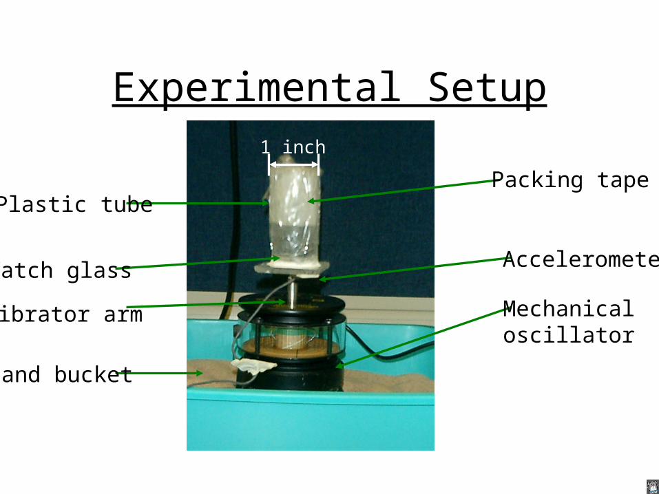
Experimental Setup
Plastic tube
Watch glass
Vibrator arm
Accelerometer
Mechanicaloscillator
Sand bucket
Packing tape
1 inch
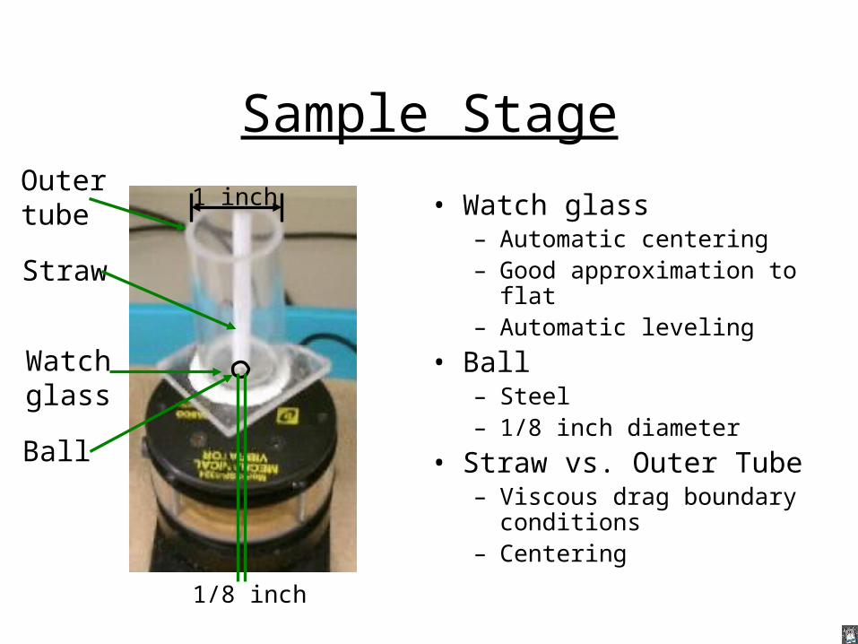
Sample Stage
• Watch glass– Automatic centering– Good approximation to flat– Automatic leveling
• Ball– Steel– 1/8 inch diameter
• Straw vs. Outer Tube– Viscous drag boundary
conditions– Centering
Watchglass
Straw
Outertube
Ball
1 inch
1/8 inch
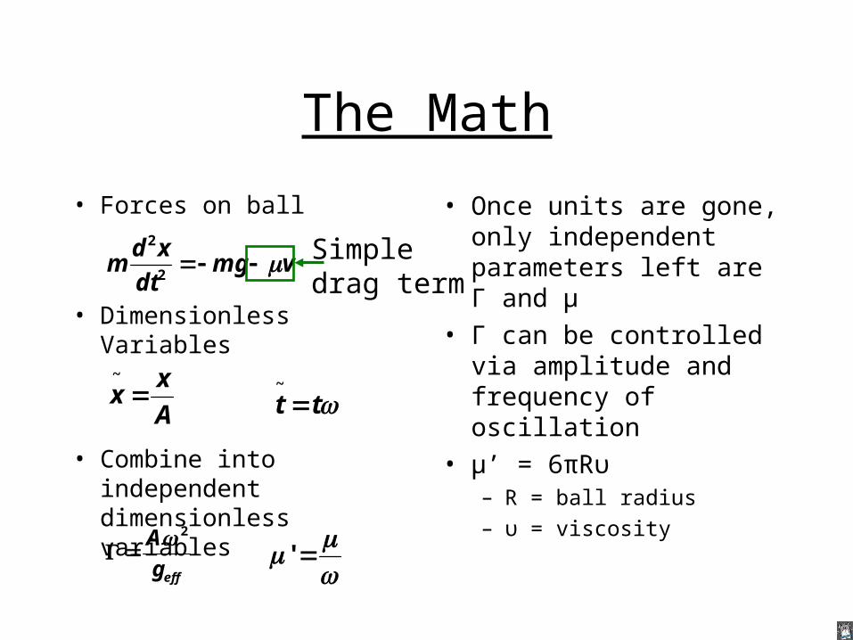
• Forces on ball
• Dimensionless Variables
• Combine into independent dimensionless variables
vmgdt
xdm
2
2
The Math
• Once units are gone, only independent parameters left are Γ and μ
• Γ can be controlled via amplitude and frequency of oscillation
• μ’ = 6πRυ– R = ball radius
– υ = viscosity
Simpledrag term
A
xx ~
tt ~
effg
A 2
'
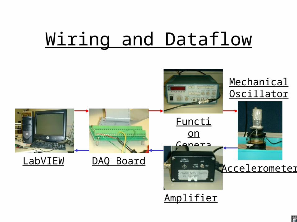
Wiring and Dataflow
LabVIEW
FunctionGenerator
Amplifier
DAQ Board
MechanicalOscillator
Accelerometer
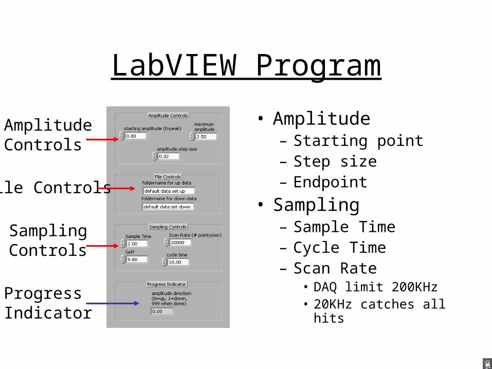
LabVIEW Program
• Amplitude– Starting point– Step size– Endpoint
• Sampling– Sample Time– Cycle Time– Scan Rate
• DAQ limit 200KHz• 20KHz catches all hits
AmplitudeControls
File Controls
SamplingControls
ProgressIndicator
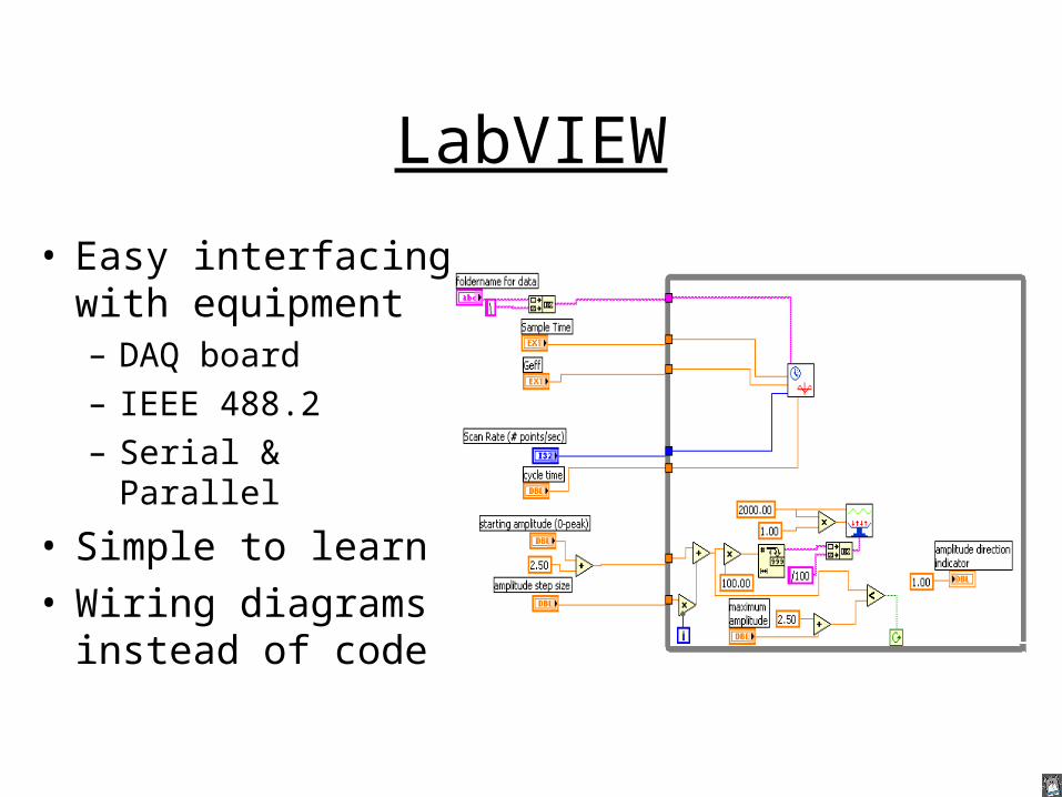
LabVIEW
• Easy interfacing with equipment– DAQ board
– IEEE 488.2
– Serial & Parallel
• Simple to learn• Wiring diagrams
instead of code
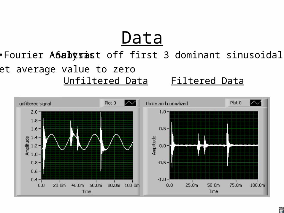
Data
Unfiltered Data Filtered Data
•Fourier Analysis •Subtract off first 3 dominant sinusoidal terms
•Set average value to zero
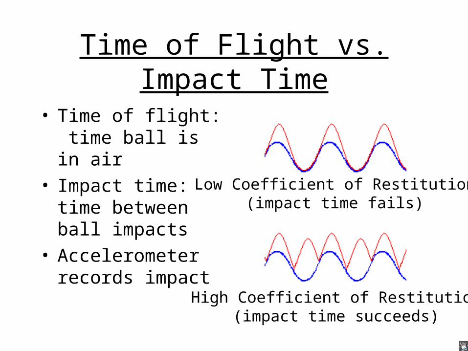
Time of Flight vs. Impact Time
• Time of flight: time ball is in air
• Impact time: time between ball impacts
• Accelerometer records impact
Low Coefficient of Restitution(impact time fails)
High Coefficient of Restitution(impact time succeeds)

Typical Data
0
0.02
0.04
0.06
0.08
0.1
0.12
0.14
0.16
0 0.5 1 1.5 2 2.5 3
Features of Graph• Data collected from
high Γ to low Γ• Single period on left• No obvious double
period region• Sharp transition to
chaosg
A 2
(s
econ
ds)
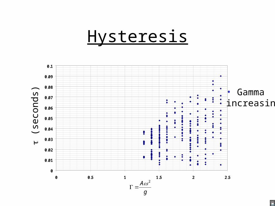
Hysteresis
0
0.01
0.02
0.03
0.04
0.05
0.06
0.07
0.08
0.09
0.1
0 0.5 1 1.5 2 2.5
g
A 2
(s
econ
ds) • Gamma
increasing
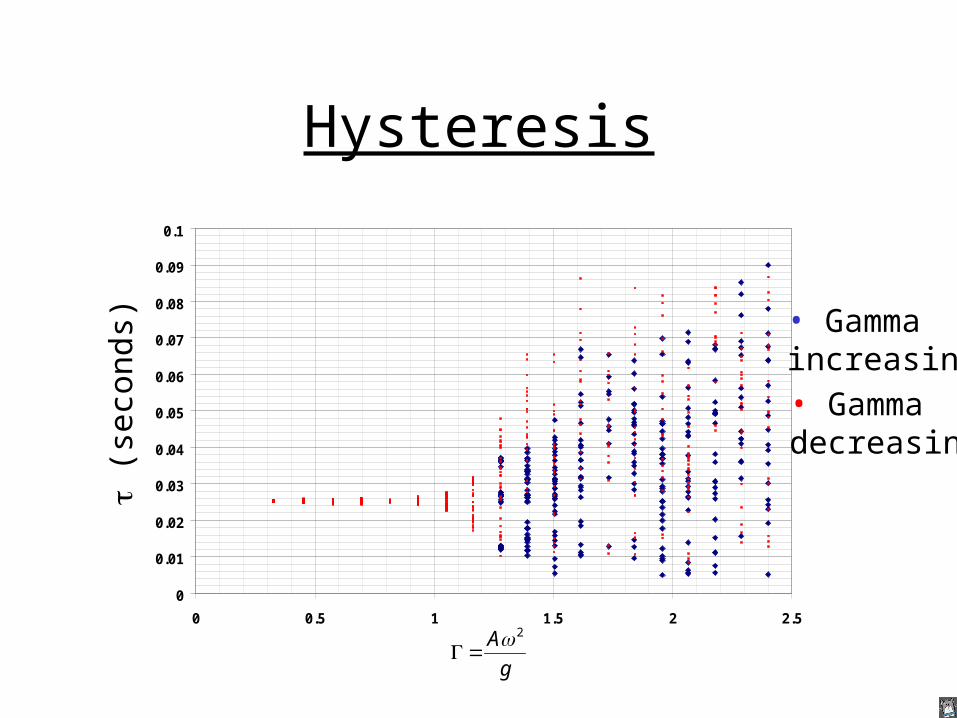
Hysteresis
0
0.01
0.02
0.03
0.04
0.05
0.06
0.07
0.08
0.09
0.1
0 0.5 1 1.5 2 2.5
g
A 2
(s
econ
ds) • Gamma
increasing• Gammadecreasing
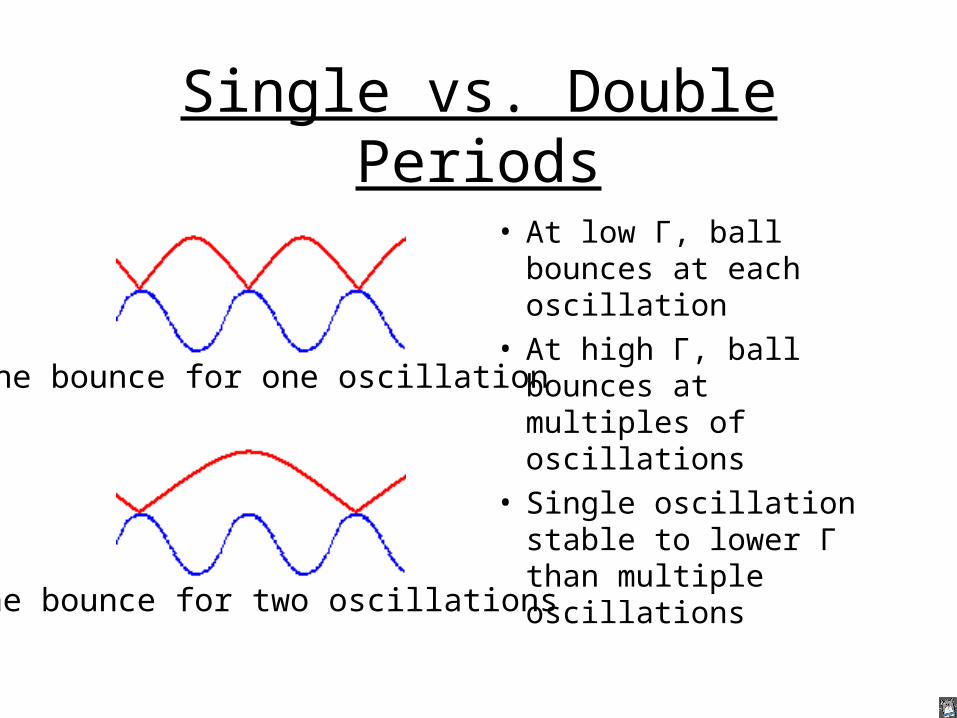
Single vs. Double Periods
• At low Γ, ball bounces at each oscillation
• At high Γ, ball bounces at multiples of oscillations
• Single oscillation stable to lower Γ than multiple oscillations
One bounce for one oscillation
One bounce for two oscillations
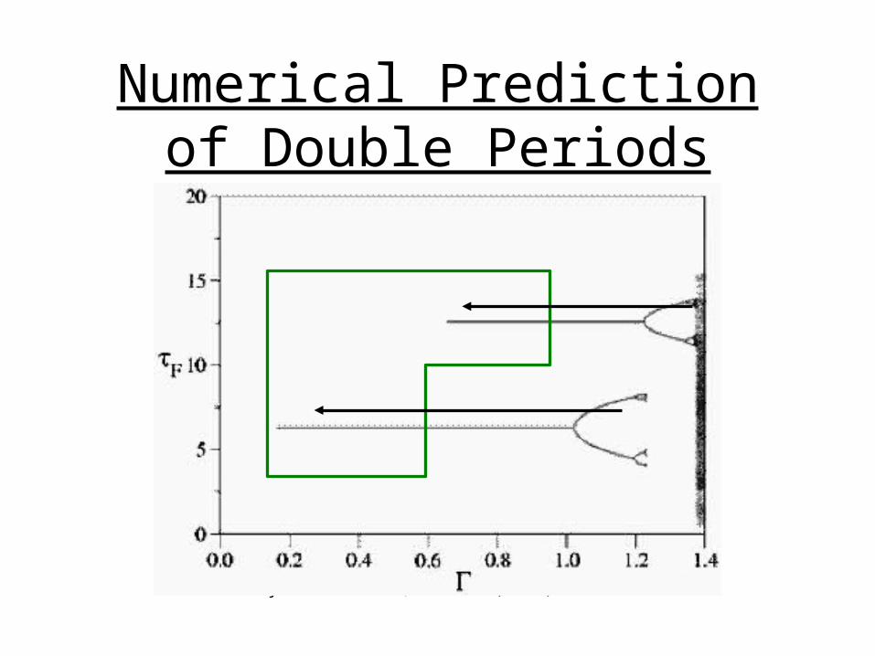
Numerical Prediction of Double Periods
Chaotic dynamics of an air-damped bouncing ball, Naylor, et. al., Phys. Rev. E 66, 057201 (2002)
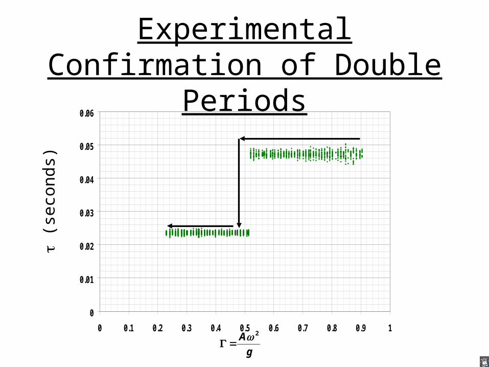
Experimental Confirmation of Double Periods
0
0.01
0.02
0.03
0.04
0.05
0.06
0 0.1 0.2 0.3 0.4 0.5 0.6 0.7 0.8 0.9 1
g
A 2
(s
econ
ds)
Future Work
• Submerge ball in viscous fluid (in progress)– Analysis of drag force important– Vary radius, viscosity, buoyant effect– ____ is only for laminar flow in infinite fluid– We may be laminar, certainly not infinite
vFd

Acknowledgements
• Scott Franklin & research group
• Kevin, Melanie, Jesus, & Ken
• RIT Department of Physics