Session 6A: Households and the Environment

Time: Thursday, August 9, 2012 PM

Paper Prepared for the 32nd General Conference of

The International Association for Research in Income and Wealth

Boston, USA, August 5-11, 2012

A Social Gradient in Households’ Environmental Policy Responsiveness?

The Case of Water Pricing in Flanders

Josefine Vanhille

For additional information please contact:

Name: Josefine Vanhille

Affiliation: University of Antwerp, Belgium

Email Address: Josefine.Vanhille@ua.ac.be

This paper is posted on the following website: http://www.iariw.org

2

Paper Prepared for the 32nd General Conference of

The International Association for Research in Income and Wealth

Boston, USA – August 5 – 11, 2012

Stream 6A: Households and the Environment

A social gradient in households’ environmental policy

responsiveness? The case of water pricing in Flanders.

Josefine VANHILLE (*)

Increasing the price of environmentally-harmful consumption constitutes a mechanism

on which many environmental policy tools are based. When evaluating efficiency aspects of

policy measures, price-based measures often perform best according to Pareto optimality. An

often expressed concern is that, when targeting households, environmental policy instruments

that are based on changing the relative price of environmentally-harmful consumption, are

bound to have regressive effects. Repeated empirical findings of this sort put the equity aspect

of this group of policy measures into question. However, the final social impact of a given

policy measure also depends of individual households’ responsiveness to the price or policy

change.

In this paper, we explore the role of socio-demographic household characteristics in the

Flemish context of water pricing. We use detailed micro-data from the Belgian part of EU-

SILC, which combines information on household income, socio-demographic characteristics,

dwelling characteristics as well as utilities expenditure.

First, we assess the importance of various household characteristics as determinants of

the quantity of water consumed by the household, employing a loglinear framework. Second,

in order to gain insight in the differential responsiveness to changes in prices across the

population, we estimate elasticities allowing variation across population subgroups, modelling

households’ water demand in a quadratic almost ideal demand system (QUAIDS) of Banks,

Blundell and Lewbel (1997).

(*) University of Antwerp - Herman Deleeck Centre for Social Policy

Sint-Jacobstraat 2

BE-2000 Antwerpen, Belgium

+ 32 3 265 53 92

josefine.vanhille@ua.ac.be

The author wishes to thank André Decoster, Rembert De Blander and Kamil Dybczak for their very

useful help with the econometric modelling issues. Of course, all remaining errors and omissions are

my own.

3

1- Introduction

Water and other utilities’ management have been focusing on demand side policies to foster a

more ‘sustainable’ (VMM 2011), ‘rational’ (Van Humbeek 2000) or ‘reasonable’ (Arbués et

al. 2010) consumption of natural resources. Increasing the relative price of environmental

goods is becoming an increasingly popular policy tool to reach this goal. Higher prices should

reflect a more correct valuation of the scarcity and/or incorporate harmful climate effects of

these goods and induce consumers to use less.

The effectiveness of price-based policies in reducing natural resource consumption depends

on the extent to which different types of consumers are sensitive to changes in the price of the

environmental good, i.e. the extent to which they react with adjusted consumption behaviour.

This is typically expressed as a price elasticity: the more negative the price elasticity, the

more the consumer will reduce consumption upon increases in price. The larger this

responsiveness, the more effective price-based policies are at attaining their goal.

For households, the last decades brought considerable price increases for water, gas, oil and

electricity. In this framework, knowledge about households’ structure of demand and

behavioural response to changes in price becomes very relevant.

It is a stylized fact that the ratio of the household’s expenses on these utilities over their

disposable income declines over the income distribution. Therefore, the often expressed

concern is that, when targeting households, environmental policy instruments that are based

on changing the relative price of environmentally-harmful consumption, are bound to have

regressive effects. This can put the policymaker in a equity-efficiency dilemma and possibly

prevent a pricing policy reflecting its scarcity, the related production and distribution costs as

well as the environmental costs of its use.

While the static distributive effects of price-based environmental policy measures are well-

documented (cf. Section 2), studies vary greatly in the way that behavioural response is taken

into account. After all, the final social impact of a given policy measure also depends of

households’ responsiveness to the price or policy change. This response can vary from

behavioural change, such as cutting back consumption, to an adjusted investment decision, by

choosing for more efficient equipment (e.g. washing machines) or installing measures to

reduce reliance on metered consumption (e.g. collecting rainwater).

Many studies that focus on distributional effects employing micro-data are of a static nature

and don’t take account of households’ responsiveness to a certain policy measure (Dresner

and Ekins 2006, Wier et al. 2005). Household demand analysis on the other hand, is often

focused on the determination of a single (mean or median) price and income elasticity of a

certain resource (fuel, electricity, water) for a given region. These can then for instance be

employed by macro and general equilibrium studies to incorporate behavioural reactions, yet

often the household sector is stylized as one (or several) representative agent(s) (e.g. Wissema

& Dellink 2007), limiting the possibility of investigating distributional, poverty or inequality

effects (Savard 2005). Some microlevel data studies on distributional effects also take

behavioural response into account by assuming it to be the same across the entire population

4

(Van Humbeek 2000). Yet, there are many reasons to believe that the vast observed

heterogeneity in energy demand translates also into differences in responsiveness of the

households to price signals and environmental policy instruments. The latter field remains

however largely understudied, with the majority of the available evidence concerns fuel

taxation.

This research aims to contribute insight from a water use perspective to this literature, to gain

insight in the extent to which households differ in their consumption patterns and in their

responsiveness to increased prices for water. After assessing the extent to which socio-

demographic characteristics play a role in determining demand, it is investigated whether they

are associated with a different responsiveness to changed policy. The latter can have

consequences for the distribution of policy-induced burdens (conservation burden and/or

financial burdens) among different socio-economic groups.

For the empirical investigation we use the case of water pricing in Flanders, the northern

region of Belgium. With the introduction of the “integrale waterfactuur” (integral water bill,

integrating costs of production and supply of drinking water on the one hand, and drainage

and cleaning of wastewater on the other hand), households have seen their water bills increase

sharply over the past few years. At the same time, discretionary control of the local authorities

about the pace at which the charges were gradually shifted towards based on metered

consumption has brought considerable variation in average prices per m³ consumed between

more “quick” (and expensive water bills) and more “slow” (and cheaper water bills) Flemish

municipalities.

In Section 2 we overview the equity-efficiency dilemma in the context of environmental

policy targeting household utilities use. Section 3 provides more detail on our case of water

pricing in Flanders, while Section 3 and 4 describe respectively the data and modelling

framework used. In Section 5 the empirical results are presented, to conclude in Section 6.

2- Environmental policy, household utilities use and the equity/efficiency dilemma

Environmental policy ranges from taxes and levies over efficiency standards, labels, to

subsidies and grants e.g. for taking conservation investment. In the paper we focus on the

literature on environmental policy operating via this pricing channel (taxation, levies, charges,

...). To reduce environmentally-harmful natural resource consumption, price increases stand

out as the most useful instruments from an efficiency point of view: an overwhelming amount

of empirical evidence shows that higher prices do reduce consumption.

Zooming in on households’ residential water demand, we are particularly interested in how

income and socio-demographic characteristics exercise an influence on the structure of

household water demand Evidence based on household-level data in this area being relatively

scarce, we also draw upon insights from other household utilities, as many parallels can be

drawn. Conceptually, this demand has common specific features. To a large extent, demand

for energy as well as for water are a derived demand: energy and water are only for a very

small part consumed as such, and for a vast majority of consumption these natural resource

goods are typically the compliment of services where, in a first instance, a number of basic

5

needs are fulfilled such as hygiene, warmth, cooking, washing, ... Furthermore, they might

also function as the compliment of more luxurious household services, from using many

electronic appliances to maintaining a swimming pool. From an environmental sustainability

point of view, energy resources as well as water are characterised by overconsumption (at

least in the developed world), and the need to reduce economy and society’s reliance on these

natural resources is widely acknowledged.

Over the past decades, the price of water and to some extent of other natural resources has

been increasingly viewed as a demand-side resource management instrument, with policy

induced price increases being widely applied in the context of households’ energy and water

consumption (for an overview of the distributional effects on households of various climate

policy measures see Buchs et al. 2011, water pricing policy measures are surveyed in Ferrara

2008). As mentioned in the introduction, the share of household disposable income to be paid

for utilities bills declines as we move up in the income distribution. Figure 1 illustrates this

stylized fact for the case of water in Flemish households.

Figure 1: Share of the “integral water bill” in household income, according to income decile,

Flanders 2009.

Source: author’s calculations on BE-SILC 2009.

Making abstraction of behavioural response, linear price increases are therefore bound to be

regressive: measured as a share of disposable income, the financial burden will be greatest in

households who pay the largest share of their income for water, typically low-income

households. Yet there are many other household characteristics that can affect household

demand for water and thus determine the share in disposable income paid for it. Reviewing

the literature, household size is consistently significant across studies when included: more

persons in the household invariably increases household water use, yet decreases water use

per person, indicating economies of scale (Höglund 1999, Arbués et al. 2004, García-Valiñas

2005). With respect to age, the evidence is unclear. On the one hand, elderly persons are more

often at home, and might therefore have a higher demand. On the other hand, they might

consume less water than younger age groups due to habits established during earlier historical

periods with less abundant conditions. The latter refers rather to a “generation” effect rather

0.0%

0.5%

1.0%

1.5%

2.0%

2.5%

% o

f d

isp

osa

ble

inco

me

income deciles

average share of household disposable income that the integral water bill represents (in %)

median share of household disposable income that the integral water bill represents (in %)

6

than a pure “age” effect. Blahdt and Kranz (2008) find evidence of this generation effect for

electricity used for lighting. Education level, employment status, whether or not there are

young children and/or teenagers in the household, these factors can hypothetically have an

influence on water use patterns, yet remain understudied due to the scarcity of data including

both water use and socio-demographic characteristics at the individual/household level.

However secondly, the final social impact of a given policy measure also depends on whether

households differ in their reaction to changed prices or policy. When distinguishing

households according to their income position, hypotheses can be made for differential

responsiveness in both directions. Low-income households might be less responsive because

they mainly use water for basic needs, and water use for these is not easily cut back. High-

income households might be more responsive to higher prices, because they are less

constraint they might use more water than strictly necessary for basic needs, and reduce this

“excess” consumption when it becomes too expensive. Alternatively, high-income households

might more easily make an upfront investment in water-saving infrastructure, that has a

certain payback time. Empirical evidence has shown that low-income families also display

greater discount rates in trading off current with future gains, and might be less likely to make

water/energy-saving investments (more efficient washing machines, rainwater collector, ...).

The other way around, low-income households might also be more responsive because they

are forced to keep a close watch on their expenses. When a good becomes significantly more

expensive, they will react with reduced consumption. High-income households on the other

hand, might not notice changes in the share of their budget that is allocated to water

consumption as much, because proportionally it is much lower, and therefore don’t react to

changed prices with adjusted consumption.

Drawing upon the empirical literature on fuel taxes, some authors find that low-income

households are more responsive to price increases than high-income households (West 2004,

Johnstone and Serret 2006). This effect mediates the regressivity of policy measures implying

real price increases. In other studies, the differences between high and low income households

are less pronounced (Brannlund and Nordstrom 2004), while Nesbakken (1999) finds that in

Norway high-income households are more responsive to energy price increases than low-

income households. To our knowledge, the only studies investigating differential

responsiveness to water price with respect to income and using household-level data are

Agthe and Billings (1987), Renwick and Archibald (1998) and Hajispyrou et al. (2002). All

three studies find higher responsiveness (more negative elasticities) for low-income

households compared to high-income households. Arbués et al. (2010) investigate differential

responsiveness according to age group. They find that smaller households have larger

elasticities (in absolute value) than larger households.

These results suggest that it is very likely that the burden of pricing policy is far from evenly

spread over different socio-economic groups. However, we need to distinguish between two

types of burdens: a financial burden and a conservation burden. To the extent that low-

incomes are more responsive to reduce their consumption in the case of a price increase, some

authors state that the financial burden following from higher prices is overstated when only

performing a static analysis without taking this differential responsiveness into account (e.g.

7

West and Williams 2002). As Buchs et al. (2011) note, however, this purely financial

perspective disguises wider fairness implications as it can be argued that poorer households,

who already have a lower consumption on average, will experience greater reductions in

terms of their broader well-being than rich households when cutting back in their

consumption levels. This refers to what Renwick and Archibald (1998) call the “conservation

burden”. When the uneven spreading of these burdens is considered unfair, policy makers can

find themselves in an equity-efficiency dilemma.

A number of responses have been formulated to overcome possible equity-efficiency

dilemmas. We identify four broad approaches. First, there is the option to compensate for

socially-adverse impacts via the personal income taxation or social insurance system, be it

with lump sum transfers or tax breaks for vulnerable households. The rationale of this type of

policy is to maintain the incentives to reduce consumption, yet compensate for socially

adverse impacts. This is a largely theoretical approach, yet Dresner and Ekins (2006)

investigate its possibilities carrying out various simulation exercises in the context of fuel

poverty in the United Kingdom. They find that while it is possible to mediate overall

regressive effects, compensation payments cannot be designed in a administratively feasible

way without leaving a substantial fraction of fuel poor households, most likely those in

deepest fuel poverty, worse off. Second, exemptions for specific household groups can be

installed within the system charging the levies. This is the option that is currently in place in

Flanders in the form of “social corrections” to the integral water bill (cfr. Section 3). The

condition is placed at the income source, so that when one of the household members receives

social assistance income, income support for the elderly or benefits from a specific type of

disability benefits in January of the starting year, the households’ water bill is automatically

adjusted to exempt the household from all wastewater charges for the entire year. Other

discount tariffs are applied in some regions in Italy, Australia and the United States (Ferrara

2008). A third view states that tariffication and charges can be made progressive on the level

of water use, in the case of water often in the form of block rate pricing. Agthe and Billings

(1987) propose substantially steeper rate progression to improve equity and encourage

conservation. However, underlying this recommendation is the assumption that “the largest

volume users are supposedly most affluent” (Agthe and Billings 1987 p.273) based on

averaged per income group. A strong association between high water consumption and wealth

has never been empirically underpinned, on the contrary, in line with previous work we also

find the variation within income groups to be much more important than the variation

between income groups (cfr. Figure 3 in Section 3). Fourth, many countries have installed

programmes of some sort to help households cope with high bills (easier payment plans, funds

to write off water debts, etc.). This type of policy, however, does not tackle adverse social

impacts an sich, but rather aims at mediating some of the most visible consequences such as

household indebtedness.

In the empirical part of this study, our aim is to unravel the influence of possibly relevant

socio-demographic characteristics such as age, household size and composition, education

level, tenure status, and especially its relative income position, on households’ water use

decisions and their price responsiveness in particular. A deeper understanding of the

8

determinants and structure of household demand for water can foster the design of demand-

side management policy measures that are both effective and equitable.

3- Case: the introduction of volumetric wastewater charges in Flanders

From January 2005 onward, the “integrated water bill” was gradually introduced for Flemish

households. The goal of this reform in the pricing structure of water was to shift the way of

charging wastewater levies from a fixed charge per tax unit to a volumetric charge based on

actual water use.

This shift can be characterized as a move closer towards “the polluter pays” principle, where

large water users will contribute more to the cost of cleaning the wastewater then small water

users. The economic rationale behind it was that the increased reliance on volumetric charge

increases the price per m³ consumed and should thus induce households to adjust their water

use behaviour and reduce consumption. For households that individually collect rainwater to

clean, water the garden and/or flush the toilet for example, a fixed wastewater charge is still in

place.

Composition of the integral water bill

The water bill for Flemish households is composed of two main parts, related to the

production and supply of drinking water on the one hand, and to the drainage and cleaning of

wastewater on the other hand.

The part of the bill for drinking water is set by the water supply company. These are public

companies and are responsible for the distribution and delivery of drinking water through a

publicly owned pipe network. There are currently 12 water suppliers operating in Flanders,

each serving a different region. As the tariff structure is set by the water supplier, pricing

structure and tariffs vary depending on the place the household lives. Generally, it is

composed of a fixed fee and a variable part that depends on the m³ consumed. Some water

companies have installed increasing or decreasing block rates (so that the tariff per m³

changes as one uses more or less water), others use a flat fee (so that the price per m³ is

independent of the amount consumed). In addition, all water companies are obliged to deliver

a first block of 15m³ per domiciled household member for free (variable tariff of 0, the fixed

fee remains in place).1

Since 2005, there is a second part of the Flemish households’ water bill which comprises two

levies for wastewater. Both consist of a flat volumetric charge based on the total m³ consumed

1 When this obligation was introduced with the 1990s reform, there were two types of reasoning for its

existence, one socially-inspired and one based on the view that it would stimulate rational water consumption among households (Van Humbeek 2000). The first argument was based on the assumption that low-income households would consume less water, thus the benefit of the free allowances would proportionally be higher for them. Policymakers also expressed their expectation that the free supply of 15m³ drinking water per person would lead to more rational water consumption patterns: as it introduces a first step towards increasing block tariff system, and therefore provides an incentive to keep consumption low. Neither of both arguments could be quantified, however.

9

(including the 15 m³ that is set free from the variable drinking water tariff). The first tariff is

determined by the municipality, the second is determined by the Flemish region, and is

therefore the same throughout Flanders. This wastewater charge should generate a revenue

reflecting the cost of the responsibilities of the municipalities and the Flemish region

respectively in the water draining and purification process. Towards this goal, wastewater

charges have been introduced gradually, rising year after year on average with a factor

reflecting a constant rate rise at the regional level of Flanders and the varying rates at the

municipality level.

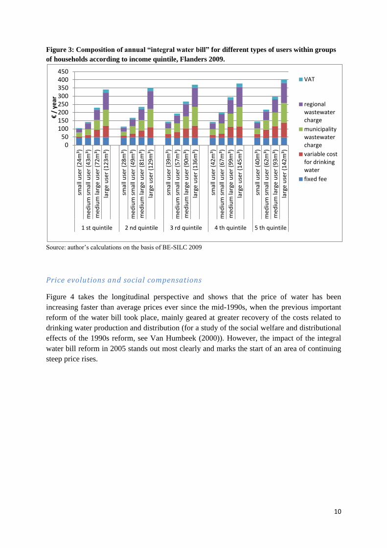
The composition of the integral water bill for different types of households is presented in

Figure 2 and 3. Figure 2 shows level of consumption and associated bill structure for small

(20th percentile), medium-small (40th percentile), medium-large (60th percentile) and large

(80th percentile) water users within families with 1 to 4 household members. In Figure 3, the

families are divided according to income quintiles from 1 (lowest income) to 5 (highest

income). Following from the different rate structures, we observe that for low-users, the fixed

fee is relatively more important, while the variable fee is proportionally less important, also

given the free 15 m³ per household member. Expectedly, there is a clear positive correlation

between household size and household water use, yet the variation within the group of

families with the same size is much larger. The same pattern appears when households are

grouped according to income quintile (Figure 3). The positive correlation is present, although

less pronounced. Again, variation between families within the same income quintile is much

larger than variation in averages between quintiles.

Figure 2: Composition of annual “integral water bill” for different types of users within groups

of households with different size, Flanders 2009.

Source: author’s calculations on the basis of BE-SILC 2009

0 50

100 150 200 250 300 350 400 450 500

smal

l use

r (2

1m

³)

med

ium

sm

all u

ser

(32

m³)

med

ium

larg

e u

ser

(45

m³)

larg

e u

ser

(82

m³)

smal

l use

r (3

6m

³)

med

ium

sm

all u

ser

(55

m³)

med

ium

larg

e u

ser

(76

m³)

larg

e u

ser

(10

9m

³)

smal

l use

r (5

3m

³)

med

ium

sm

all u

ser

(83

m³)

med

ium

larg

e u

ser

(11

2m

³)

larg

e u

ser

(15

6m

³)

smal

l use

r (6

3m

³)

med

ium

sm

all u

ser

(95

m³)

med

ium

larg

e u

ser

(12

7m

³)

larg

e u

ser

(17

6m

³)

1 person hh 2 person hh 3 person hh 4 person hh

€ /

yea

r

VAT

regional wastewater charge municipality wastewater charge variable cost for drinking water fixed fee

10

Figure 3: Composition of annual “integral water bill” for different types of users within groups

of households according to income quintile, Flanders 2009.

Source: author’s calculations on the basis of BE-SILC 2009

Price evolutions and social compensations

Figure 4 takes the longitudinal perspective and shows that the price of water has been

increasing faster than average prices ever since the mid-1990s, when the previous important

reform of the water bill took place, mainly geared at greater recovery of the costs related to

drinking water production and distribution (for a study of the social welfare and distributional

effects of the 1990s reform, see Van Humbeek (2000)). However, the impact of the integral

water bill reform in 2005 stands out most clearly and marks the start of an area of continuing

steep price rises.

0 50

100 150 200 250 300 350 400 450

smal

l use

r (2

4m

³)

med

ium

sm

all u

ser

(43

m³)

med

ium

larg

e u

ser

(72

m³)

larg

e u

ser

(12

3m

³)

smal

l use

r (2

8m

³)

med

ium

sm

all u

ser

(49

m³)

med

ium

larg

e u

ser

(81

m³)

larg

e u

ser

(12

9m

³)

smal

l use

r (3

9m

³)

med

ium

sm

all u

ser

(57

m³)

med

ium

larg

e u

ser

(90

m³)

larg

e u

ser

(13

6m

³)

smal

l use

r (4

2m

³)

med

ium

sm

all u

ser

(67

m³)

med

ium

larg

e u

ser

(99

m³)

larg

e u

ser

(14

5m

³)

smal

l use

r (4

0m

³)

med

ium

sm

all u

ser

(62

m³)

med

ium

larg

e u

ser

(93

m³)

larg

e u

ser

(14

2m

³)

1 st quintile 2 nd quintile 3 rd quintile 4 th quintile 5 th quintile

€ /

ye

ar

VAT

regional wastewater charge

municipality wastewater charge

variable cost for drinking water

fixed fee

11

Figure 4: Evolution of the price of water for households compared to harmonized index of

consumer prices, Belgium/Flanders 1998-2011.

Source: based on statistics from Belgostat and VMM (2011).

Since the first introduction of the wastewater charges in 2005, average water bill has risen

further with 67% (for an average single person households) to 96% (for an average 5-person

household) between 2005 and 2011 (VMM 2011). Already in the 1990s reform, concerns

about the affordability of water in socially-vulnerable households led to the exemption of

certain groups in the regional and municipal wastewater levy. At the time of writing, a

household qualifies for these so-called “social corrections” when at least one member of the

household receives a social assistance allowance or pension or a specific disability benefit. In

their case, the household only pays for the drinking water component of the bill. Households

that qualify for the social corrections but don’t have individual metering of their use, receive a

lump sum payment to compensate for the cost of the charges. Since 2008, the exemption

and/or compensation payments are automatically allocated to the eligible households, before,

the households had to apply for it. In 2009, the social corrections applied to about 5% of the

household water bills (VMM 2010).

When taking an average household of 2.37 household members and an annual water

consumption of 88m³, the annual water bill in 2009 varied, depending on where the household

lives (municipality and drinking water supply region), between 189 and 335 euro, or a ratio of

1.8 between the most ‘cheap’ and ‘expensive’ water regions. The variation in tariffication

between different drinking water companies produces a variation ratio of 1.5. The

introduction of the municipal wastewater charge tariff added significantly to the price

variation, as its own variation ratio amounted to 2.4 in 2009 (for the average household).

It is this variation in prices (both average and marginal) that we will use to estimate our

demand system for water and derive price and income elasticities across different groups of

Flemish households.

50

75

100

125

150

175

200

225

250

275

1998 1999 2000 2001 2002 2003 2004 2005 2006 2007 2008 2009 2010 2011

ind

exe

d p

rice

evo

luti

on

evolution of average price per m³ drinking water (for households) [data 1998-2004]

evolution of integral water bill at fixed consumption of average household [data 2000-2011]

harmonized index of consumer prices ("gezondheidsindex")

12

4- Data

The most recent available version of the Belgian SILC data (survey year 2009, with income

data referring to 2008) provides us with the micro data (ADSEI) which, compared to the

EUROSTAT EU-SILC database, contain more detailed information on housing costs. In the

Belgian questionnaire, the household respondent responds to three questions relating to water:

first, it is asked whether the households pays for the cost of water. If the household answers

yes, the respondent is asked to provide an estimation of the monthly cost of water. If the

respondent can’t give an answer for water separately, the possibility is foreseen that the

respondents gives the aggregate total of water and other utilities such as gas or electricity.

We restrict our sample to households living in Flanders, who report to pay for water and are

able to indicate a value for the account. The latter condition implies that we can’t use 14% of

the households in the sample, who don’t report a valid value. Partly, this is caused by item

non-response, and partly by a reflection of reality, as there is still a share of privately-rented

accommodation that doesn’t have separate metering. Reported values that appear unreliable

because they are extremely low (<1st percentile) or extremely high (>99th percentile) are

dropped from the sample as well. Our final sample used for the analysis contains 2741

households.

As mentioned, the data contains the respondents’ estimation of the average monthly cost for

water. Using the annual equivalent and the necessary information about the place where the

household lives (and thus which drinking water tariff and which municipal wastewater charge

applies) we calculate the m³ of water consumed associated with this annual bill using an

iterative procedure. We also account for social corrections because nearly all the income

components that determine eligibility were surveyed. However, it appears that the question on

the specific disability allowance that gives right to the exemption of wastewater charges, was

not accurately answered, resulting in an underrepresentation of households eligible for

socially corrected water bills. Overall, we obtain a socially-corrected water bill for only 1.9%

of the households in our sample (n=47). In part this is due to inaccuracies in recording the

exact income components each individual receives, but also we observe that households who

would be eligible for social corrections are slightly more present (2.3%) in the group that we

had to drop from the sample because there was no reliable information on their water bill.

This again illustrates the difficulties to obtain full information on more precarious population

groups in nation-wide representative surveys such as EU-SILC.

The main advantage of our dataset is that is combines information on yearly water bills with

detailed information on income and socio-demographic characteristics and some basic

information on housing situation for a representative sample of the Flemish population. This

direct link at the household level between water use, characteristics of the house and

information on the household and its member, is quite rare in household water demand

analysis. The majority of studies uses data at aggregated (typically community) level (e.g.

Martínez-Espiñeira 2002, Nauges and Thomas 2003, Mazzanti and Montini 2006). Studies

with household-level data are typically obtained from water company records, implying that

13

the number of independent variables is often quite limited. Studies that included an indicator

for household income or wealth have worked so far with proxies such as average net income

in the neighbourhood (aggregated data studies) or a measure of fiscal value of the property

(e.g. Hewitt and Hanemann 1995; Arbués et al. 2010). In the analysis, we keep in mind that

representativeness might be slightly affected by the non-negligible item non-response

observed.

The main disadvantage of our dataset is that we work with reported euro instead of metered

m³, which automatically introduces a certain error because of possible inaccuracy in the

answer of the household respondent. We assume that this error is randomly distributed and

does not affect overall results. Also, there is the risk that the calculate of the m³ associated

with the reported bill are wrong when we don’t observe a fulfilled eligibility condition in the

data when in reality it is there, and therefore social corrections are automatically allocated.

Finally, we don’t observe in the data whether the household collects its own rainwater. Given

the small proportion of houses in Flanders that have the infrastructure to do this, we further

make abstraction of the special treatment of individual water collectors.

5- Modelling framework

A number of different empirical approaches have been developed in the literature on

modelling households’ residential water demand. Methods used vary in the nature of the data

used (microlevel or aggregated, (repeated) cross-sections or panel data), in the specification of

the model, in the choice of dependent and independent variables, and in specification of

crucial parameters, most notably price. For an excellent overview of the methodological

issues, see Arbués et al. (2003) and Worthington and Hoffmann (2008). After the

specification of our model in the following paragraph, we focus on those issues raised that are

relevant in the context of our analysis: the inclusion of socio-demographic and housing

characteristics, the use of household-level cross-sectional data, the specification of the price

variable, and the modelling of free allowances.

QUAIDS system

We model households’ demand for water using the tools from consumer demand analysis.

Our framework is a function , where water consumption is related to price (P)

and other factors (Z, housing characteristics, socio-demographic characteristics). We opt for

the relatively simple, comprehensive yet flexible framework of the Quadratic Almost Ideal

Demand System (QUAIDS) developed by Banks, Blundell and Lewbel (1997), extending the

Almost Ideal Demand System of Deaton and Muellbauer (1980) to allow for quadratic Engel

curves.

Starting point are the households expenditure shares ( ) given by , where

reflects the price and the quantity of good , and stands for the household’s total

expenditure on all goods in the demand system.

In the QUAIDS system each expenditure share can be estimated as

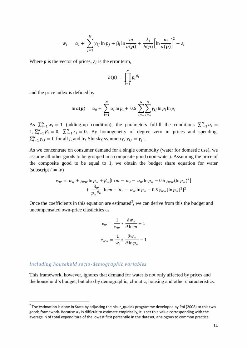
14

Where p is the vector of prices, is the error term,

and the price index is defined by

As (adding-up condition), the parameters fulfill the conditions

, ,

. By homogeneity of degree zero in prices and spending,

for all j, and by Slutsky symmetry, .

As we concentrate on consumer demand for a single commodity (water for domestic use), we

assume all other goods to be grouped in a composite good (non-water). Assuming the price of

the composite good to be equal to 1, we obtain the budget share equation for water

(subscript )

Once the coefficients in this equation are estimated2, we can derive from this the budget and

uncompensated own-price elasticities as

Including household socio-demographic variables

This framework, however, ignores that demand for water is not only affected by prices and

the household’s budget, but also by demographic, climatic, housing and other characteristics.

2 The estimation is done in Stata by adjusting the nlsur_quaids programme developed by Poi (2008) to this two-

goods framework. Because is difficult to estimate empirically, it is set to a value corresponding with the average ln of total expenditure of the lowest first percentile in the dataset, analogous to common practice.

15

It is very likely that there are systematic differences in consumption behaviour between

households with different characteristics. The role of demographic determinants in demand

analysis was already brought to attention by Pollak and Wales (1981). More recently, also

Moro and Sckokai (2000), Blow (2003) and Dybczak et al. (2010) show empirical evidence

for the importance of the role of demographic determinants in demand analysis. Leaving out

demographic factors from aggregate demand analysis may produce misleading results.

In the QUAIDS system, we can introduce variation in the intercept and slope parameters by

allowing them to depend on household characteristics in each budget share equation of the

demand system. Thus, parameters α, β, and λ are allowed to vary depending on the household

characteristics, while impact of prices reflected in γ is assumed to be same over households.

With this approach, we follow Moro and Sckokai (2000) and Dybczak et al. (2010). In this

respect our model also differs from earlier QUAIDS analysis on water by Hajispyrou et al.

(2002), as they only allow the intercept to vary with socio-demographic and technical

characteristics.

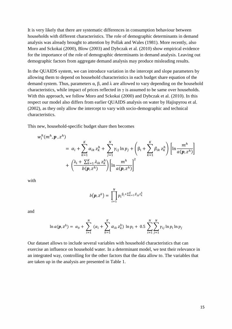
This new, household-specific budget share then becomes

with

and

Our dataset allows to include several variables with household characteristics that can

exercise an influence on household water. In a determinant model, we test their relevance in

an integrated way, controlling for the other factors that the data allow to. The variables that

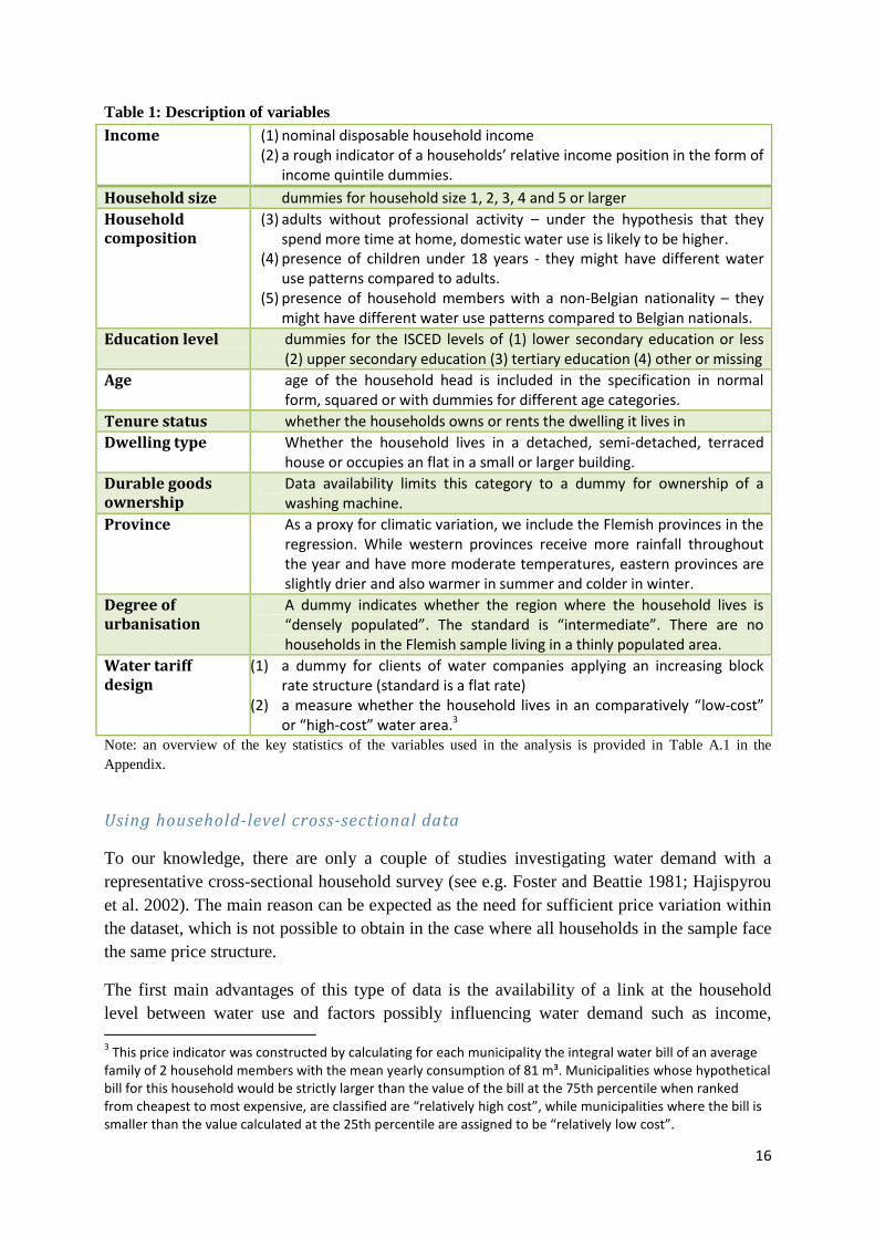
are taken up in the analysis are presented in Table 1.

16

Table 1: Description of variables

Income (1) nominal disposable household income (2) a rough indicator of a households’ relative income position in the form of

income quintile dummies.

Household size dummies for household size 1, 2, 3, 4 and 5 or larger

Household composition

(3) adults without professional activity – under the hypothesis that they spend more time at home, domestic water use is likely to be higher.

(4) presence of children under 18 years - they might have different water use patterns compared to adults.

(5) presence of household members with a non-Belgian nationality – they might have different water use patterns compared to Belgian nationals.

Education level dummies for the ISCED levels of (1) lower secondary education or less (2) upper secondary education (3) tertiary education (4) other or missing

Age age of the household head is included in the specification in normal form, squared or with dummies for different age categories.

Tenure status whether the households owns or rents the dwelling it lives in

Dwelling type Whether the household lives in a detached, semi-detached, terraced house or occupies an flat in a small or larger building.

Durable goods ownership

Data availability limits this category to a dummy for ownership of a washing machine.

Province As a proxy for climatic variation, we include the Flemish provinces in the regression. While western provinces receive more rainfall throughout the year and have more moderate temperatures, eastern provinces are slightly drier and also warmer in summer and colder in winter.

Degree of urbanisation

A dummy indicates whether the region where the household lives is “densely populated”. The standard is “intermediate”. There are no households in the Flemish sample living in a thinly populated area.

Water tariff design

(1) a dummy for clients of water companies applying an increasing block rate structure (standard is a flat rate)

(2) a measure whether the household lives in an comparatively “low-cost” or “high-cost” water area.3

Note: an overview of the key statistics of the variables used in the analysis is provided in Table A.1 in the

Appendix.

Using household-level cross-sectional data

To our knowledge, there are only a couple of studies investigating water demand with a

representative cross-sectional household survey (see e.g. Foster and Beattie 1981; Hajispyrou

et al. 2002). The main reason can be expected as the need for sufficient price variation within

the dataset, which is not possible to obtain in the case where all households in the sample face

the same price structure.

The first main advantages of this type of data is the availability of a link at the household

level between water use and factors possibly influencing water demand such as income, 3 This price indicator was constructed by calculating for each municipality the integral water bill of an average

family of 2 household members with the mean yearly consumption of 81 m³. Municipalities whose hypothetical bill for this household would be strictly larger than the value of the bill at the 75th percentile when ranked from cheapest to most expensive, are classified are “relatively high cost”, while municipalities where the bill is smaller than the value calculated at the 25th percentile are assigned to be “relatively low cost”.

17

housing characteristics and socio-demographic characteristics of the household. The second

advantage is that the cross-sectional variation in price structure within the small and relatively

homogeneous region of Flanders allow us to estimate income and price elasticities that reflect

more long term responsiveness (when also the capital stock can be adjusted), while estimates

based on panel data over a relatively short period (a couple of years) are assumed to reflect

short term elasticities (when the capital stock is largely fixed and changes only result from

adjusted consumption behaviour).

Expectedly, estimates for short term elasticities are often smaller in absolute value than

estimates for long term elasticities, as responses to price changes are found to be significantly

larger in the long run, when households have had the time to adjust their capital stock to a

certain change in real prices, than when capital stock is fixed and only consumption behaviour

is variable.

From a policy perspective, it is the long-term elasticity which is most relevant when one is

interested in sustainably reducing levels of water use. We would however be careful to

assume our estimates to be real long-term elasticities, as at the time of the survey (2009) the

policy changes that have led to the observed price variation in the data have been introduced

over the course of only four years (since 2005), making it less probable that all households

who faced the steepest price increases already fully adjusted their capital stock.

Specification of the price variable

In the literature, both average and marginal prices have been used in modelling water demand,

and the debate on to which water prices consumer respond in the case of complex water price

structures is not settled yet (Nordin 1976, Nieswiadomy and Molina 1991, Arbués et al. 2003)

Foster and Beattie (1981) argue that the water tariffication structure with different block rates

and the inclusion of wastewater charges lead to too high information costs for households to

be able to respond to marginal prices when deciding on their water consumption. Shin (1985)

elaborates this argument empirically with respect to electricity bills.

The choice clearly matters, as shown in Table 2, as the average price is determined by the

level of consumption (the lower a households’ consumption, the more important the fixed fee

proportionally, and the higher the average price). The marginal price however, is much less

dependent on the level of consumption (once the household consumes more than the allocated

free m³) and reflects in the first place regional differences between drinking water companies

and municipal wastewater charges.

18

Table 2: average and marginal price at different percentiles of household water use.

water use in m³ median of average price median of marginal price

5th percentile 15 4.68 3.53

10th percentile 22 4.44 3.24

25th percentile 38 3.57 3.53

50th percentile 66 3.41 3.54

75th percentile 106 3.29 3.53

90th percentile 156 3.19 3.31

95th percentile 196 3.13 3.29

Source: author’s calculations on BE-SILC.

Arbués et al. (2003) and Worthington and Hoffman (2008) map the wide variation in price

specifications present in the literature of the past decades.

In line with basic economic theory on consumer behaviour and with more recent practice

(Dandy 1997, Hajispyrou et al. 2002, Nataraj and Hanemann 2011), we opt to use marginal

prices calculated as the price of a hypothetical m³ water consumption in addition to the

households’ current use. In the majority of the cases, this is the flat rate that applies to all

consumption in excess of the free allowance of 15m³ per household member. In the few cases

of households using less than their allocated free allowance, it is substantially lower. In the

case where households face an increasing block rate price structure, this corresponds to the

marginal tariff of the block in which their consumption is situated.

The modelling of free allowances.

The econometric specificities of modelling free allowances are treated in Dandy et al. (1997).

The problem of a zero marginal price as long as households consume less than the allocated

15 m³ per household member is not applicable in the Flemish case, as the free allocation only

concerns the part of the bill related to drinking water. As the levies for wastewater are being

charged from the first m³ onwards, there is no consumption with a zero marginal price. As

long as a household remains within the free drinking water band, the marginal price is of

course considerably lower than when the marginal price includes both the drinking water and

the wastewater rate.

6- Results

We start this section with a descriptive outline of the relationship between household demand

for water and a number of technical characteristics of the water pricing system, and some

social, economic and demographic characteristics of the household. Next, we assess which

factors are driving household water demand in a multivariate determinant model, and finally

turn to estimated elasticities from the QUAIDS demand system.

19

Descriptive associations between water use and socio-demographic, dwelling

and regional variables.

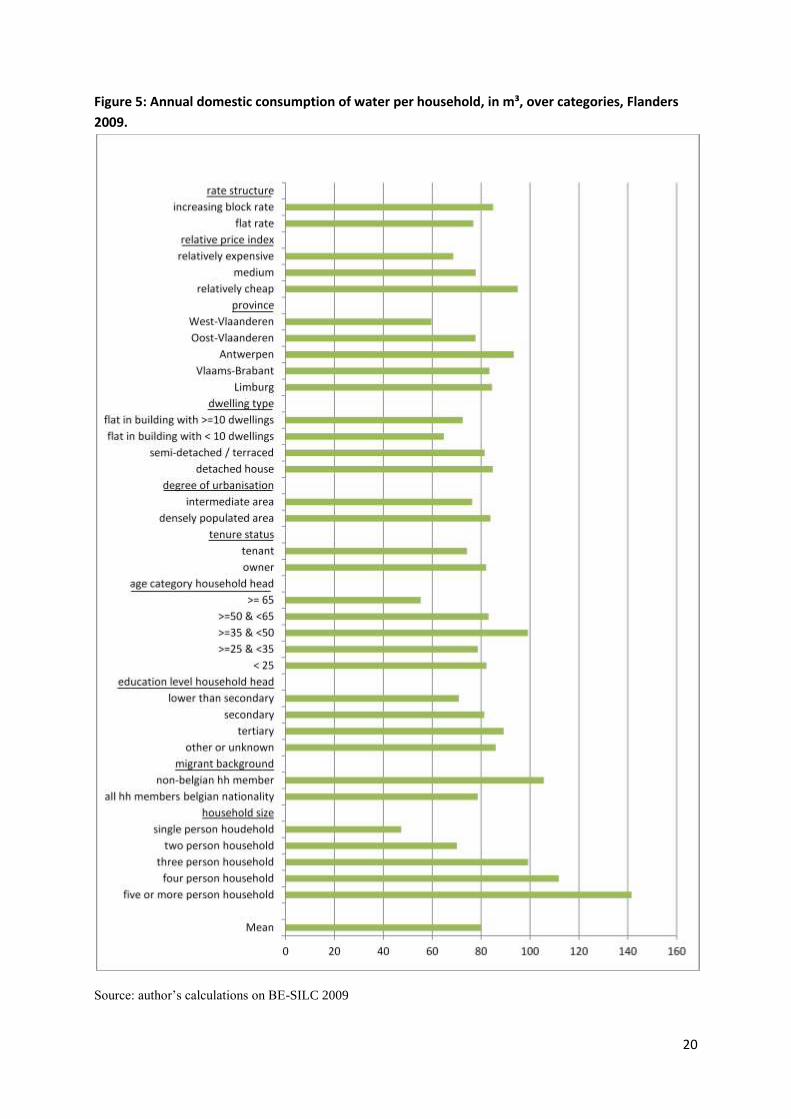
Figure 5 and 6 show average water use over households according to the characteristics

described in Section 5. In Figure 5, this is done with the variable of household water use, in

Figure 6 with water use per household member. Doing this, a number of patterns are reversed,

showing the importance of controlling for household size (and other variables) while

assessing the influence of other characteristics.

In general, most relationships show the expected direction. In relatively expensive water

regions, less water is used, while more is being used is relatively cheap regions. Households

living in the Flanders’ most western province, West-Vlaanderen, use less water, while in

Antwerpen water use per household is higher than in the other provinces. Households living

in a flat consume a smaller amount of water on average, however, when expressed as m³ per

household member, they use more than households in (semi-)detached or terraced houses,

showing the influence of the fact that households living in an apartment tend to be smaller in

size. Households living in densely populated areas use slightly more water, per household as

well as per person. On average, owner-occupier households use more water than tenants,

however, again the relationship is inversed when looking at average use per household

member. The observed differences when looking at the relationship between age of the

household head and household water use disappears entirely when measured per household

member. When distinguishing households according to education level, the same observation

holds. The presence of someone with a non-Belgian nationality in the household appears to be

positively correlated with water use both when measured at the household level as when

measured at the individual level. Then finally, the relationship between household size and

water use displays the most outspoken pattern. When water consumption is measured per

household, there is a strong positive correlation, while we observe a consistent negative

relationship between household size and water use per individual water consumption, clearly

marking the presence of economies of scale (see also Höglund 1999, Arbués et al. 2004,

García-Valiñas 2005).

20

Figure 5: Annual domestic consumption of water per household, in m³, over categories, Flanders

2009.

Source: author’s calculations on BE-SILC 2009

21

Figure 6: Annual domestic consumption of water per household member, in m³, over categories,

Flanders 2009.

Source: author’s calculations on BE-SILC 2009

0 10 20 30 40 50 60

Mean

five or more person household four person household

three person household two person household

single person houdehold household size

all hh members belgian … non-belgian hh member

migrant background other or unknown

tertiary secondary

lower than secondary education level household head

< 25 >=25 & <35 >=35 & <50 >=50 & <65

>= 65 age category household head

owner tenant

tenure status densely populated area

intermediate area degree of urbanisation

detached house semi-detached / terraced

flat in building with < 10 … flat in building with >=10 …

dwelling type Limburg

Vlaams-Brabant Antwerpen

Oost-Vlaanderen West-Vlaanderen

province relatively cheap

medium relatively expensive relative price index

flat rate increasing block rate

rate structure

22

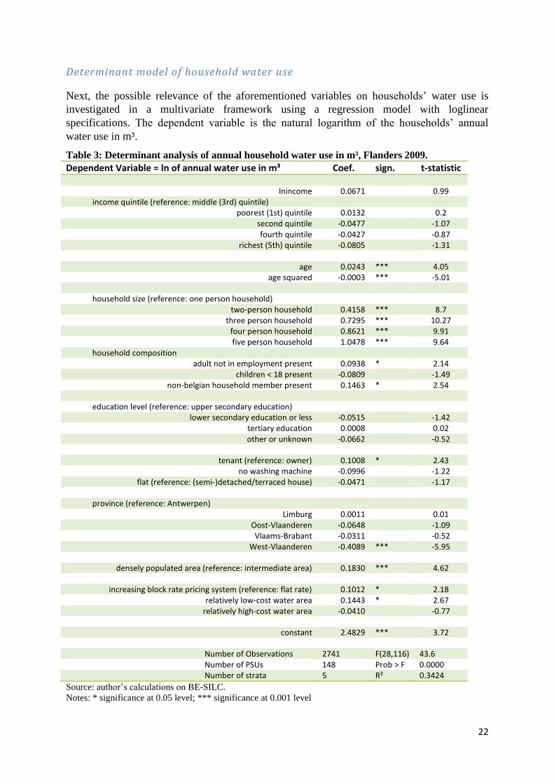
Determinant model of household water use

Next, the possible relevance of the aforementioned variables on households’ water use is

investigated in a multivariate framework using a regression model with loglinear

specifications. The dependent variable is the natural logarithm of the households’ annual

water use in m³.

Table 3: Determinant analysis of annual household water use in m³, Flanders 2009.

Dependent Variable = ln of annual water use in m³ Coef. sign. t-statistic

lnincome 0.0671 0.99 income quintile (reference: middle (3rd) quintile)

poorest (1st) quintile 0.0132 0.2 second quintile -0.0477 -1.07 fourth quintile -0.0427 -0.87

richest (5th) quintile -0.0805 -1.31

age 0.0243 *** 4.05 age squared -0.0003 *** -5.01

household size (reference: one person household)

two-person household 0.4158 *** 8.7 three person household 0.7295 *** 10.27

four person household 0.8621 *** 9.91 five person household 1.0478 *** 9.64

household composition adult not in employment present 0.0938 * 2.14

children < 18 present -0.0809 -1.49 non-belgian household member present 0.1463 * 2.54

education level (reference: upper secondary education)

lower secondary education or less -0.0515 -1.42 tertiary education 0.0008 0.02 other or unknown -0.0662 -0.52

tenant (reference: owner) 0.1008 * 2.43

no washing machine -0.0996 -1.22 flat (reference: (semi-)detached/terraced house) -0.0471 -1.17

province (reference: Antwerpen)

Limburg 0.0011 0.01 Oost-Vlaanderen -0.0648 -1.09 Vlaams-Brabant -0.0311 -0.52

West-Vlaanderen -0.4089 *** -5.95

densely populated area (reference: intermediate area) 0.1830 *** 4.62

increasing block rate pricing system (reference: flat rate) 0.1012 * 2.18 relatively low-cost water area 0.1443 * 2.67

relatively high-cost water area -0.0410 -0.77

constant 2.4829 *** 3.72

Number of Observations 2741 F(28,116) 43.6 Number of PSUs 148 Prob > F 0.0000 Number of strata 5 R² 0.3424

Source: author’s calculations on BE-SILC.

Notes: * significance at 0.05 level; *** significance at 0.001 level

23

Controlling for these observable characteristics, many relationships turn out not to be

significant, implying they were driven by an uneven distribution of other relevant

characteristics over the categories. Age and household size appear to be two most pronounced

deterministic variables. Living in a densely populated area as well as living in the province of

West-Vlaanderen also appears to have a strongly significant (<0.001) influence on

households’ water consumption. Further, significant relationships at the 5% level could be

identified from the variable indicating whether households are tenants, the presence of adults

that are not employed and/or non-Belgian nationals, whether households face an increasing

block rate pricing system, and live in a low-cost water area. The latter is also found to be

significantly correlated with the level of water consumption in Hajispyrou et al. (2002).

Remarkably, in this determinant framework we could not identify any significant relationship

between income and the m³ of water consumed. It is difficult to compare this outcome to

other studies on determinants of water demand, as the vast majority of the existing studies

employ aggregated data mostly at the community level (see e.g. Schleich and Hillenbrand for

an example and literature overview). Here, average water consumption are matched with

averages of other demand-related characteristics, such as per capita income per community.

This approach conceals many possible household-level determinants, in particular socio-

demographic characteristics, that can be correlated with income. Studies on water demand

that do employ individual household data often don’t have household income and other socio-

demographic characteristics at their disposal in the dataset either and therefore have to use a

proxy for income, typically a fiscal indicator of the value of the dwelling (Arbués et al. 2004,

2010, García-Valiñas 2005, Arbués and Villanúa 2006). Nevertheless, studies that are more

similar in methodology to ours, such as Hajispyrou, also find an influence of income although

its significance is not mentioned. Studies with a more comparable methodology to ours are

found in the literature investigating determinants of energy (space heating, electricity) also do

find a statistically significant positive influence of income on energy use (Rehdanz 2007,

Meier and Rehdanz 2010, Jamasb and Meier 2010).

QUAIDS demand model and household responsiveness

First, we model household demand for water using the QUAIDS framework, using the

information on price, water expenditure and total income at the household level only. As

presented in Table X, the estimated values for all parameters, including lambda, are highly

significant, indicating the appropriateness of allowing for non-linear or quadratic Engel

curves.

Table 4: QUAIDS parameter estimates

Coef. sign. Standard error z-value

0.02971 *** 0.000964 30.82 -0.03462 *** 0.000749 -46.23 0.00249 *** 0.000662 3.76 0.01004 *** 0.000268 37.45

Source: author’s calculations on BE-SILC 2009.

24

The estimated values for these parameters generate an income elasticity estimate of 0.62

evaluated at the population average, and a uncompensated (compensated) price elasticity

estimate of -0.615 (-0.609).

In an extension of this model, these variables that proved most deterministic in water demand

(age and household size, province of west-vlaanderen and densely populated area) plus

quintile dummies enter in the demand model. These variables enter the model by means of

dummy variables for the province of west-vlaanderen, for densely populated area, for 5 age

categories for the household head (16-24; 25-34; 35-49; 50-64; >=65), for the number of

family members (1; 2; 3; 4; 5 or more), and for 5 income quintiles. We assume that living in

West-Vlaanderen or in a densely populated area can affect the intercept of water use, while

both intercept and slope parameters are allowed to vary with age category of the household

head, household size and income quintile.

The estimated parameters are reported in Table A.2 in the appendix. None of the allowed

interactions with the age dummies in the model are significant, implying that the dummies fail

to capture the more complex relationship found in the determinant model. The household size

and income quintile interactions do result in small but significant differences in the parameter

estimates for each category in α, β and λ. Also the dummies for West-Vlaanderen and densely

populated area significantly alter α a little bit.

The estimates allow us to calculate the price elasticity4 evaluated at the average of each

category, controlling for different distribution in the other category (e.g. uneven distribution

of household size over the income quintiles). The estimates are reported in Table X. For each

category, the price elasticities are negative, significantly different from zero, and between 0

and 1, indicating that water is an inelastic good. The results suggest that low-income

households as well as smaller families have a significantly higher price responsiveness (more

negative price elasticity) than high-income families and larger families. The difference

between income groups is slightly more pronounced than the difference between households

of different sizes, but in both cases confidence intervals at the 95% level for the estimates for

the lowest and the highest group are not overlapping.

Table 5: own-price water elasticities according to income quintile and household size, Flanders

2009.

income quintile estimate sign standard error z-value 95% C.I.

1 -0.76948 *** 0.0304947 -25.23 -0.82925 -0.70971

2 -0.67896 *** 0.0522478 -13 -0.78136 -0.57656

3 -0.57768 *** 0.0649505 -8.89 -0.70498 -0.45038

4 -0.49989 *** 0.0834761 -5.99 -0.6635 -0.33628

5 -0.25182 * 0.1121718 -2.24 -0.47168 -0.03197

household size estimate sign standard error z-value 95% C.I.

1 -0.74459 *** 0.0433935 -17.16 -0.82964 -0.65954

4 The estimated values for the income elasticities failed to be significantly different from zero for each category

and came with too large confidence intervals to be regarded as reliable estimates.

25

2 -0.62415 *** 0.0612374 -10.19 -0.74417 -0.50413

3 -0.55395 *** 0.0715989 -7.74 -0.69428 -0.41362

4 -0.50767 *** 0.0802024 -6.33 -0.66486 -0.35047

>=5 -0.34044 *** 0.0731229 -4.66 -0.48376 -0.19712

Source: author’s calculations on BE-SILC 2009.

Notes: * significance at 0.05 level; *** significance at 0.001 level

This finding is in line with other empirical studies investigating differential responsiveness

(Agthe and Billings (1987), Renwick and Archibald (1998), Hajispyrou et al. 2002, Arbués et

al. 2010). The first three studies find higher responsiveness (more negative elasticities) for

low-income households compared to high-income households, ranging between -0.57 (lowest

income group) to 0.40 (high income group) in the study by Agthe and Billings (1987),

between -0.53 (lowest income households) and -0.11 (highest income households) in the

study by Renwick and Archibald (1998) and between -0.79 (lowest income group) and -0.39

(highest income group) in Hajispyrou et al. (2002).

Arbués et al. (2010) investigate differential responsiveness according to age group. They find

that smaller households have larger elasticities (in absolute value) than larger households,

ranging from below -1 for small households to -0.26 for large households.

With respect to differentiating according to relative income position, it provides support for

the hypotheses that low-income households are more responsive to price changes because

they are forced to keep a close watch on their expenses. When a good becomes significantly

more expensive, they react more than high-income households by reducing their consumption.

High-income households on the other hand, might not notice changes in the share of their

budget that is allocated to water consumption as much, because proportionally it represents a

smaller part of their income, and therefore react much less to changed prices with adjusted

consumption.

With respect to differentiating according to household size, our result imply that small

households are better able to adjust to changes in the price of water than large households.

Which mechanism is driving this result, is not a priori clear. Arbués et al. (2010) propose two

explanations. A first explanation is related to the existence of endogenous transaction costs

related to the introduction and spread of new practices that improve the efficiency of water

appliances like taps, tanks, washing machines and dish washers. They hypothesize that these

transaction costs might be higher in larger households, because the organisation and

supervision of household activities is more complex. Secondly, they propose that household

size affects the capacity of the household to improve the efficiency of its water use practices:

Usually, white goods utilization is less efficient in small households than larger ones due to

the fact that they are more often used below full capacity, thereby not fully exploiting

economies of scale related to their use. Therefore, it is hypothesized, small households will be

better able to obtain efficiency improvements in water consumption in response to exogenous

incentives, while larger household are already making use of these economies of scale.

26

7- Conclusions

The effectiveness of price-based policies in reducing natural resource consumption depends

on the extent to which different types of consumers are sensitive to changes in the price of the

environmental good. Using the case of volumetric wastewater charges in Flanders, we employ

observed price heterogeneity between different water pricing areas to model a quadratic

almost ideal demand system, allowing us to estimate households’ differential price

responsiveness.

We find that all households are responsive to prices, regardless of their relative income

position or size. Yet the significant differences in elasticities between household groups

suggest that the financial and conservation burden of the installed water pricing policy are not

distributed evenly across the population. Lower income households and smaller size

households are found to be more responsive to increased prices than higher income

households and larger size households.

Future research should assess both social effects in an integrated way, quantifying the

distribution of financial incidence as well as the distribution of the conservation burden within

a coherent framework. This would allow us to make policy recommendations on the

possibilities to overcome the equity-efficiency dilemma typically observed when installing

environmental policy measures geared at increasing the price of natural resources that are at

the same time consumed by households to fulfil a number of basic needs.

References

Agthe, D. E. and R. B. Billings (1987). "Equity, Price Elasticity and household income under

increasing block rates for water." American Journal of Economics and Sociology

46(3): 273-286.

Arbués, F., R. Barberán, et al. (2004). "Price impact on urban residential water demand: A

dynamic panel data approach." Water Resources Research 40(11).

Arbu s, F., M. a. . Garc a-Valiñas, et al. (2003). "Estimation of residential water demand: a

state-of-the-art review." Journal of Socio-Economics 32(1): 81-102.

Arbués, F. and I. Villanua (2006). "Potential for pricing policies in water resource

management: Estimation of urban residential water demand in Zaragoza, Spain."

Urban Studies 43(13): 2421-2442.

Arbués, F., I. Villanúa, et al. (2010). "Household size and residential water demand: an

empirical approach." Australian Journal of Agricultural and Resource Economics

54(1): 61-80.

Banks, J., R. Blundell, et al. (1997). "Quadratic engel curves and consumer demand." Review

of Economics and Statistics 79(4): 527-539.

Blow, L. (2003). Demographics in Demand Systems. IFS Working Papers. London, Institute

for Fiscal Studies.

Dalhuisen, J. M., R. Florax, et al. (2003). "Price and income elasticities of residential water

demand: A meta-analysis." Land Economics 79(2): 292-308.

Dandy, G., T. Nguyen, et al. (1997). "Estimating residential water demand in the presence of

free allowances." Land Economics 73(1): 125-139.

27

Deaton, A. and J. Muellbauer (1980). "An almost ideal demand system." American Economic

Review 70(3): 312-326.

Dybczak, K., P. Tóth, et al. (2010). Effects of Price Shocks to Consumer Demand. Estimating

the QUAIDS Demand System on Czech Household Budget Survey Data. Working

Paper Series. Prague, Czech National Bank.

Espey, M., J. Espey, et al. (1997). "Price elasticity of residential demand for water: A meta-

analysis." Water Resources Research 33(6): 1369-1374.

Ferrara, I. (2008). Residential Water Demand. Household Behaviour and the Environment.

OECD. Paris, OECD Publishing.

Foster, H. S., Jr. and B. R. Beattie (1981). "On the Specification of Price in Studies of

Consumer Demand under Block Price Scheduling." Land Economics 57(4): 624-629.

García-Valiñas, M. A. (2005). "Efficiency and equity in natural resources pricing: A proposal

for urban water distribution service." Environmental & Resource Economics 32(2):

183-204.

Hajispyrou, S., P. Koundouri, et al. (2002). "Household demand and welfare: implications of

water pricing in Cyprus." Environment and Development Economics 7(04): 659-685.

Hewitt, J. A. and W. M. Hanemann (1995). "A discrete-continuous choice approach to

residential water demand under block rate pricing." Land Economics 71(2): 173-192.

Höglund, L. (1999). "Household demand for water in Sweden with implications for a

potential tax on water use." Water Resources Research 35(2): 3853-3863.

Jamasb, T. and H. Meier (2010). Household Energy Expenditure and Income Groups:

Evidence from Great Britain. Cambridge Working Papers in Economics, Faculty of

Economics, University of Cambridge.

Kriström, B. (2008). Residential Energy Demand. Household Behaviour and the

Environment. OECD. Paris, OECD Publishing.

Martinez-Espiñeira, R. (2002). "Residential Water Demand in the Northwest of Spain."

Environmental and Resource Economics 21(2): 161-187.

Mazzanti, M. and A. Montini (2006). "The determinants of residential water demand:

empirical evidence for a panel of Italian municipalities." Applied Economics Letters

13(2): 107-111.

Meier, H. and K. Rehdanz (2010). "Determinants of residential space heating expenditures in

Great Britain." Energy Economics 32(5): 949-959.

Moro, D. and P. Sckokai (2000). "Heterogeneous preferences in household food consumption

in Italy." European Review of Agricultural Economics 27(3): 305-323.

Nataraj, S. and W. M. Hanemann (2011). "Does marginal price matter? A regression

discontinuity approach to estimating water demand." Journal of Environmental

Economics and Management 61(2): 198-212.

Nauges, C. and A. Thomas (2003). "Long-run Study of Residential Water Consumption."

Environmental and Resource Economics 26(1): 25-43.

Nesbakken, R. (1999). "Price sensitivity of residential energy consumption in Norway."

Energy Economics 21(6): 493-515.

Nieswiadomy, M. L. and D. J. Molina (1989). "Comparing Residential Water Demand

Estimates under Decreasing and Increasing Block Rates Using Household Data." Land

Economics 65(3): 280-289.

Nieswiadomy, M. L. and D. J. Molina (1991). "A Note on Price Perception in Water Demand

Models." Land Economics 67(3): 352-359.

Olmstead, S. M., W. M. Hanemann, et al. (2007). "Water demand under alternative price

structures." Journal of Environmental Economics and Management 54(2): 181-198.

Poi, B. P. (2002). "From the help desk: Demand system estimation." Stata Journal 2(4): 403-

410.

28

Poi, B. P. (2008). "Demand-system estimation: Update." Stata Journal 8(4): 554-556.

Pollak, R. A. and T. J. Wales (1981). "Demographic Variables in Demand Analysis."

Econometrica 49(6): 1533-1551.

Rehdanz, K. (2007). "Determinants of residential space heating expenditures in Germany."

Energy Economics 29(2): 167-182.

Renwick, M. E. and S. O. Archibald (1998). "Demand Side Management Policies for

Residential Water Use: Who Bears the Conservation Burden." Land Economics 74(3):

343-359.

Savard, L. (2005). "Poverty and Inequality Analysis within a CGE Framework: A

Comparative Analysis of the Representative Agent and Microsimulation Approaches."

Development Policy Review 23(3): 313-331.

Schleich, J. and T. Hillenbrand (2009). "Determinants of residential water demand in

Germany." Ecological Economics 68(6): 1756-1769.

Shin, J.-S. (1985). "Perception of Price When Price Information Is Costly: Evidence from

Residential Electricity Demand." The Review of Economics and Statistics 67(4): 591-

598.

Van Humbeek, P. (2000). The Distributive Effects of Water Price Reform on Households in

th Flanders Region of Belgium. The Political Economy of Water Pricing Reforms. A.

Dinar. New York, Oxford University Press.

VMM (2010). Evaluatie bovengemeentelijke en gemeentelijke bijdrage 2008/2009. Brussel,

VLaamse Milieu Maatschappij - Economisch Toezichthouder.

VMM (2011). Watermeter 2011 - drinking water production and supply in figures. Brussel,

Vlaamse Milieu Maatschappij - Waterregulator.

Wissema, W. and R. Dellink (2007). "AGE analysis of the impact of a carbon energy tax on

the Irish economy." Ecological Economics 61(4): 671-683.

Worthington, A. C. and M. Hoffman (2008). "An Empirical Survey of Residential Water

Demand Modelling." Journal of Economic Surveys 22(5): 842-871.

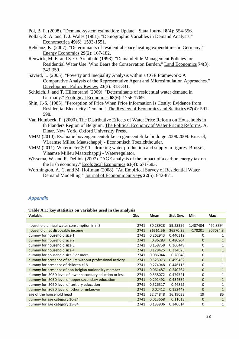
Appendix

Table A.1: key statistics on variables used in the analysis

Variable Obs Mean Std. Dev. Min Max

household annual water consumption in m3 2741 80.28928 59.23396 1.487404 462.8894 household net disposable income 2741 36561.56 26570.39 -178201 907034.3 dummy for household size 1 2741 0.262943 0.440312 0 1 dummy for household size 2 2741 0.36283 0.480904 0 1 dummy for household size 3 2741 0.159758 0.366449 0 1 dummy for household size 4 2741 0.128425 0.334623 0 1 dummy for household size 5 or more 2741 0.086044 0.28048 0 1 dummy for presence of adults without professional activity 2741 0.525073 0.499462 0 1 dummy for presence of children <18 2741 0.274048 0.446115 0 1 dummy for presence of non-belgian nationality member 2741 0.061487 0.240264 0 1 dummy for ISCED level of lower secondary eduction or less 2741 0.358072 0.479521 0 1 dummy for ISCED level of upper secondary education 2741 0.291492 0.454532 0 1 dummy for ISCED level of tertiary education 2741 0.326317 0.46895 0 1 dummy for ISCED level of other or unknown 2741 0.02412 0.153448 0 1 age of the household head 2741 52.74848 16.19033 19 85 dummy for age category 16-24 2741 0.013668 0.11613 0 1 dummy for age category 25-34 2741 0.133906 0.340614 0 1

29

dummy for age category 34-49 2741 0.310914 0.462952 0 1 dummy for age category 50-64 2741 0.282512 0.450303 0 1 dummy for age category 65 and older 2741 0.259 0.438166 0 1 dummy for tenant household 2741 0.225029 0.417677 0 1 dummy for apartment 2741 0.164582 0.370871 0 1 dummy for no owned washing machine 2741 0.048977 0.215859 0 1 dummy for densely populated area 2741 0.524958 0.499468 0 1 dummy for Antwerp province 2741 0.26835 0.443181 0 1 dummy for Limburg province 2741 0.129718 0.336054 0 1 dummy for Oost-Vlaanderen province 2741 0.232848 0.422723 0 1 dummy for Vlaams-Brabant province 2741 0.174633 0.379722 0 1 dummy for West-Vlaanderen province 2741 0.194453 0.395851 0 1 dummy for household facing increasing block rate price structure

2741 0.426701 0.494688 0 1

dummy for comparatively low water cost area 2741 0.233183 0.422935 0 1 dummy for comparatively average water cost area 2741 0.561858 0.496249 0 1 dummy for comparatively high cost area 2741 0.20496 0.403746 0 1

Source: BE-SILC 2009

Table A.2 Parameter estimates for QUAIDS model extended with socio-demographic

characteristics, Flanders 2009.

Coefficient sign. standard error z-value

0.016145 *** 0.004538 3.56

-0.03567 *** 0.009695 -3.68

0.003132 *** 0.000532 5.89

0.019885 *** 0.004969 4

0.013002 *** 0.00117 11.11

0.021709 *** 0.003446 6.3

0.021803 *** 0.004968 4.39

0.037222 *** 0.006738 5.52

-0.01316 *** 0.00304 -4.33

-0.01031 * 0.005149 -2

-0.02195 ** 0.008067 -2.72

-0.04764 *** 0.006401 -7.44

0.008467 0.005145 1.65

0.007837 0.004674 1.68

0.00419 0.00458 0.91

0.008808 0.004524 1.95

0.000625 * 0.000304 2.06

-0.00295 *** 0.000366 -8.08

-0.02168 *** 0.002109 -10.28

-0.02905 *** 0.004668 -6.22

-0.02918 *** 0.00622 -4.69

-0.04982 *** 0.008565 -5.82

0.040656 *** 0.006008 6.77

0.036089 *** 0.007896 4.57

0.051421 *** 0.010049 5.12

0.078288 *** 0.005707 13.72

30

-0.00653 0.010406 -0.63

-0.00645 0.009845 -0.66

-0.00148 0.009748 -0.15

-0.013 0.0097 -1.34

0.008876 *** 0.001086 8.17

0.010396 *** 0.001704 6.1

0.010548 *** 0.00205 5.15

0.016347 *** 0.002618 6.24

-0.02252 *** 0.002722 -8.27

-0.02141 *** 0.002856 -7.5

-0.02643 *** 0.003088 -8.56

-0.03351 *** 0.001543 -21.71

0.000242 0.005064 0.05

0.000544 0.004905 0.11

-0.00104 0.004878 -0.21

0.00372 0.004875 0.76

Source: author’s calculations on BE-SILC 2009.

Notes: * significance at 0.05 level; ** significance at 0.01 level; *** significance at 0.001 level. hs2-5 refers to

household size 2 to 5 or more, reference group is household size 1. iq2-5 refers to income quintile 2 to 5,

reference group is income quintile 1. ac2-5 refers to age category 2 to 5, reference category is age category 1. dp

refers to densely populated, wv refers to the West-Vlaanderen province.