BOOTSTRAP FOR PANEL DATA�

Bertrand HOUNKANNOUNON

Université de Montréal, CIREQ

April 26, 2008

Preliminary

Abstract

This paper considers bootstrap methods for panel data. Theoretical results are given for thesample mean. It is shown that simple resampling methods (i.i.d., individual only or temporal only)are not always valid in simple cases of interest, while a double resampling that combines resamplingin both individual and temporal dimensions is valid. This approach also permits to avoid multiplesasymptotic theories that may arise in large panel models. In particular, it is shown that thisresampling method provides valid inference in the one-way and two-way error component modelsand in the factor models. Simulations con�rm these theoretical results.

JEL Classi�cation : C15, C23.

Keywords : Bootstrap, Panel Data Models.

�I am grateful to Benoit Perron and Silvia Gonçalves for helpful comments. All errors are mine. Financial supportfrom the Department of Economics, Université de Montréal and CIREQ is gratefully acknowledged. Address forcorrespondance : Université de Montréal, Département de Sciences Economiques, C.P. 6128, succ. Centre-Ville,Montréal, Qc H3C 3J7, Canada. E-mail : b.hounkannounon@umontreal.ca.

1

1 Introduction

The true probability distribution of a test statistic is rarely known. Generally, its asymptotic lawis used as approximation of the true law. If the sample size is not large enough, the asymptoticbehaviour of the statistics could lead to a poor approximation of the true one. Using bootstrapmethods, under some regularity conditions, it is possible to obtain a more accurate approximationof the distribution of the test statistic. Original bootstrap procedure has been proposed by Efron(1979) for statistical analysis of independent and identically distributed (i.i.d.) observations. It is apowerful tool for approximating the distribution of complicated statistics based on i.i.d. data. Thereis an extensive literature for the case of i.i.d. observations. Bickel & Freedman (1981) establishedsome asymptotic properties for bootstrap. Freedman (1981) analyzed the use of bootstrap for leastsquares estimator in linear regression models.

In practice, observations are not i.i.d. Since Efron (1979) there is an extensive research toextend bootstrap to statistical analysis of non i.i.d. data. Wild bootstrap is developed in Liu(1988) following suggestions in Wu (1986) and Beran (1986) for independent but not identicallydistributed data. Several bootstrap procedures have been proposed for time series. The two mostpopular approaches are sieve bootstrap and block bootstrap. Sieve bootstrap attempts to modelthe dependence using a parametric model. The idea behind it is to postulate a parametric formfor the data generating process, to estimate the parameters and to transform the model in orderto have i.i.d. elements to resample. The weakness of this approach is that results are sensitiveto model misspeci�cation and the attractive nonparametric feature of bootstrap is lost. On theother hand, block bootstrap resamples blocks of consecutive observations. In this case, the useris not obliged to specify a particular parametric model. For an overview of bootstrap methodsfor dependent data, see Lahiri (2003). Application of bootstrap methods to several indices datais an embryonic research �eld. The expression "several indices data" regroups : clustered data,multilevel data, and panel data.

The term "panel data" refers to the pooling of observations on a cross-section of statisticalunits over several periods. Because of their two dimensions (individual -or cross-sectional- andtemporal), panel data have the important advantage to allow to control for unobservable hetero-geneity, which is a systematic di¤erence across individuals or periods. For an overview about paneldata models, see for example Baltagi (1995) or Hsiao (2003). There is an abounding literatureabout asymptotic theory for panel data models. Some recent developments treat of large panels,when temporal and cross-sectional dimensions are both important. Paradoxically, literature aboutbootstrap for panel data is rather restricted. In general, simulation results suggest that some re-sampling methods work well in practice but theoretical results are rather limited or exposed withstrong assumptions. As references of bootstrap methods for panel models, it can be quoted Bellmanet al. (1989), Andersson & Karlsson (2001), Carvajal (2000), Kapetanios (2004), Focarelli (2005),Everaert & Pozzi (2007) and Herwartz (2006; 2007). In error component models, Bellman et al.(1989) uses bootstrap to correct bias after feasible generalised least squares. Andersson & Karlsson(2001) presents bootstrap resampling methods for one-way error component model. For two-wayerror component models, Carvajal (2000) evaluates by simulations, di¤erent bootstrap resamplingmethods. Kapetanios (2004) presents theoretical results when cross-sectional dimension goes toin�nity, under the assumption that cross-sectional vectors of regressors and errors terms are i.i.d..This assumption does not permit time varying regressors or temporal aggregate shocks in errorsterms. Focarelli (2005) and Everaert & Pozzi (2007) uses bootstrap to reduce bias in dynamic panelmodels with �xed e¤ects when T is �xed and N goes to in�nity, bias quoted by Nickell (1981).Herwartz (2006; 2007) deliver a bootstrap version to Breusch-Pagan test in panel data modelsunder cross-sectional dependence.

2

This paper aims to expose some theoretical results on various bootstrap methods for panel data.Theoretical results and simulation exercises concern the sample mean. The paper is organized asfollows. In the second section, di¤erent panel data models are presented. Section 3 presents �vebootstrap resampling methods for panel data. The fourth section presents theoretical results,analyzing validity of each resampling method. In section 5, simulation results are presented andcon�rm theoretical results. The sixth section concludes.

2 Panel Data Models

It is practical to represent panel data as a rectangle. By convention, in this document, rows corre-spond to the individuals and columns represent time periods. A panel dataset with N individualsand T time periods is represented by a matrix Y of N rows and T columns. Y contains thus NTelements. yit is i0s observation at period t:

Y(N;T )

=

0BBBB@y11 y12 ::: ::: y1Ty21 y22 ::: ::: y2T::: ::: ::: ::: :::::: ::: ::: :: :::yN1 yN2 :: ::: yNT

1CCCCAConsider a panel model without regressor.

yit = � + �it (2.1 )

� is an unknown parameter and �it a random variable. Inference is about the parameter � andits estimator is the sample mean. It is usual in a �rst step to establish the validity of bootstrap forthe sample mean, before investigating more complicated statistics. Assumptions about �it de�nedi¤erent panel data models. The speci�cations commonly used can be summarized by (2.2) underassumptions below.

�it = �i + ft + �iFt + "it (2.2 )

AssumptionsA1 : (�1; �2; ::::::; �N ) � i:i:d:

�0; �2�

�, �2� 2 (0;1)

A2 : fftg is a stationary and strong �-mixing process1 with E (ft) = 0, 9 � 2 (0;1) :

E jftj2+� <1,1Xj=1

� (j)�=(2+�) <1 , and V1f =

1Xh=�1

Cov (ft; ft+h) 2 (0;1)

A3 : (�1; �2; ::::::; �N ) � i:i:d:�0; �2�

�, �2� 2 (0;1)

A4 : f"itgi=1:::N; t=1::T � i:i:d:�0; �2"

�, �2" 2 (0;1)

A5 : fFtg is a stationary and strong �-mixing process with E (Ft) = 0, 9 � 2 (0;1) :

E jFtj2+� <1,1Xj=1

� (j)�=(2+�) <1 , and V1F =1X

h=�1Cov (Ft; Ft+h) 2 (0;1)

A6 : The �ve series are independent.

These assumptions can seem strong. They are made in order to have strong convergence andto simplify demonstrations. Considering special cases with di¤erent combinations of processes in

1See Appendix 7 for de�nition of an �-mixing process.

3

(2.2), gives the following panel data models : i.i.d. panel model, one-way error component model,two-way error component model and factor model.

Iid panel model

yit = � + "it (2.3 )

This speci�cation is the most simple panel model. Even if observations have a panel structure,they exhibit no dependence in cross-sectional or temporal dimension.

One-way ECM

yit = � + �i + "it (2.4)

yit = � + ft + "it (2.5)

Two speci�cations are considered. The term, one-way error component model (ECM), comesfrom the structure of error terms : only one kind of heterogeneity, that is systematic di¤erencesacross cross-sectional units or time periods, is taken into account. The speci�cation 2.4 (resp. 2.5)allows to control unobservable individual (resp. temporal) heterogeneity. The speci�cation (2.4)is called individual one-way ECM, (2.5) is temporal one-way ECM. It is important to emphasizethat here, unobservable heterogeneity is a random variable, not a parameter to be estimated. Thealternative is to use �xed e¤ects model in which heterogeneity must be estimated.

Two-way ECM

yit = � + �i + ft + "it (2.6 )

Two-way error component model allows to control for individual and temporal heterogeneity,hence the term two-way. Like in one-way ECM, individual and temporal heterogeneities are randomvariables. Classical papers on error component models include Balestra & Nerlove (1966), Fuller &Battese (1974) and Mundlak (1978).

Factor Model

yit = � + �i + �iFt + "it (2.7)

yit = � + �iFt (2.8)

Two speci�cations are considered. In (2.7), the di¤erence with one-way ECM, is the term �iFt.The product allows the common factor Ft to have di¤erential e¤ects on cross-section units. Thisspeci�cation is used by Bai & Ng (2004), Moon & Perron (2004) and Phillips & Sul (2003). It is away to introduce dependence among cross-sectional units. An other way is to use spatial model inwhich, the structure of the dependence can be related to geographic, economic or social distance(see Anselin (1988))2. The second speci�cation, (2.8) allows to anylize properly the factor e¤ect.

2Bootstrap methods studied in this paper do not take into account spatial dependence. Reader insterested byresampling methods for spatial data, can see for example Lahiri (2003), chap. 12.

4

3 Resampling Methods

This section presents the bootstrap methodology and �ve ways to resample panel data.

Bootstrap Methodology

From initial N � T data matrix Y , create a new matrix Y � by resampling with replacementelements of Y: This operation must be repeated B times in order to have B + 1 pseudo-samples :fY �b gb=1::B+1. Statistics are computed with these pseudo-samples in order to make inference. Theprobability measure induced by the resampling method conditionally on Y is noted P � . E� () andV ar� () are respectively expectation and variance associated to P �. In this paper, inference is about� and consists in building con�dence intervals and testing hypothesis. There is close link betweencon�dence interval and hypthosis tests : each can be seen as the dual program of the other. Theresampling methods used to compute pseudo-samples are exposed below.

I.i.d. Bootstrap

In this document i.i.d bootstrap refers to original bootstrap as de�ned by Efron (1979). It wasdesigned for one dimensional data, but it�s easy to adapt it to panel data. For a N � T matrixY , i.i.d. resampling is the operation of constructing a N � T matrix Y � where each element y�it isselected with replacement from Y: Conditionally on Y , all the elements of Y � are independent andidentically distributed. There is a probability 1=NT that each y�it is one of the NT elements yit ofY: The mean of Y � obtained by i.i.d. bootstrap is noted y�iid.

Individual Bootstrap

For a N � T matrix Y , individual resampling is the operation of constructing a N � T matrixY � with rows obtained by resampling with replacement rows of Y: Conditionally on Y , the rowsof Y � are independent and identically distributed. Contrary to i.i.d. bootstrap case, y�it cannottake any value. y�it can just take one of the N values fyitgi=1;:::N . The mean of Y � obtained byindividual bootstrap is noted y�ind:

Temporal Bootstrap

For N � T matrix Y , temporal resampling is the operation of constructing a N � T matrixY � with columns obtained by resampling with replacement colums of Y: Conditionally on Y , thecolumns of Y � are independent and identically distributed. y�it can just take one of the T valuesfyitgt=1;:::T . The mean of Y � obtained by temporal bootstrap is noted y

�temp:

Block Bootstrap

Block bootstrap for panel data is a direct accommodation of non-overlapping block bootstrapfor time series, due to Carlstein (1986). The idea is to resample in temporal dimension, notsingle period like in temporal bootstrap case, but blocks of consecutive periods in order to capturetemporal dependence. Assume that T = Kl, with l the length of a block, then there are K non-overlapping blocks. ForN�T matrix Y , block bootstrap resampling is the operation of constructing

5

a N�T matrix Y � with columns obtained by resampling with replacement, theK blocks of columnsof Y: The mean of Y � obtained by block bootstrap is noted y�bl. Note that temporal bootstrap is aspecial case of block bootstrap, when l = 1: Moving block bootstrap (Kunsch (1989), Liu & Singh(1992)), circular block bootstrap (Politis & Romano (1992)) and stationary block bootstrap (Politis& Romano (1994)) can also be accommodated to panel data.

Double Resampling Bootstrap

For a N � T matrix Y , double resampling is the operation of constructing a N � T matrixY �� with columns and rows obtained by resampling columns and rows of Y: The mean of Y �� isnoted y��: Two schemes are explored. The �rst scheme is a combination of individual and temporalbootstrap. The second scheme is a combination of individual and block bootstrap. The term doublecomes from the fact that the resampling can be made in two steps. In a �rst step, on dimension istaken into account : from Y , an intermediate matrix Y � is obtained. An other resampling is made inthe second dimension : from Y � the �nal matrix Y �� is obtained. Carvajal (2000) and Kapetanios(2004) improve this resampling method by Monte Carlo simulations, but give no theoretical support.Double stars �� are used to distinguish estimator, probability measure, expectation and varianceinduced by double resampling.

4 Theoretical Results

This section presents theoretical results about resampling methods exposed in section 3, usingmodels speci�ed in section 2.

Multiple Asymptotics

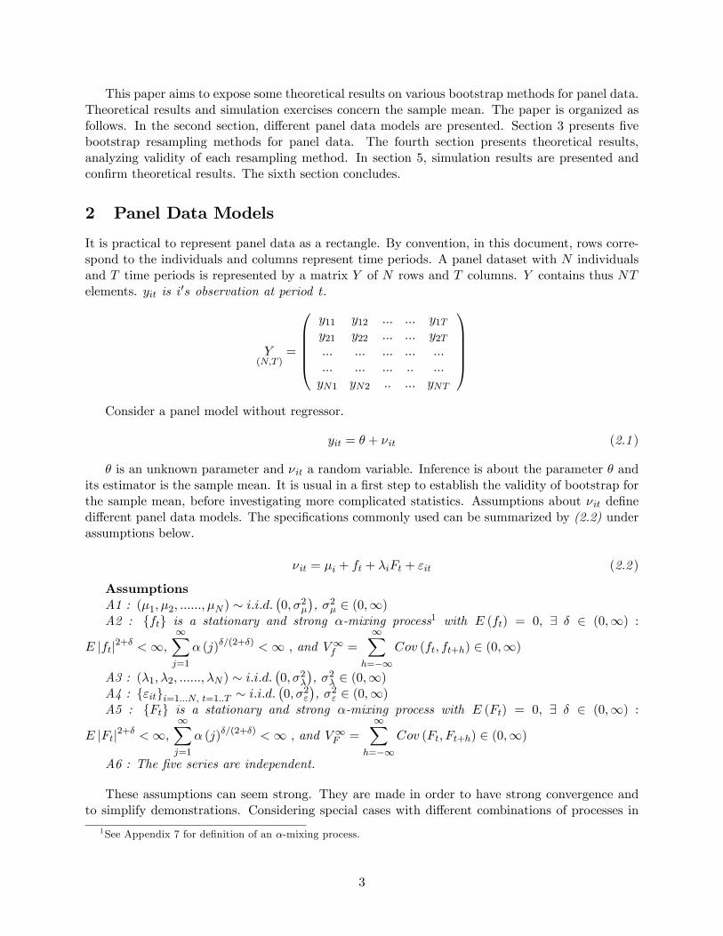
In the study of asymptotic distributions for panel data, there are many possibilities. One indexcan be �xed and the other goes to in�nity or N and T go to in�nity. In the second case, how Nand T go to in�nity, is not always without consequence. Hsiao (2003 p. 296) distinguishes threeapproaches : sequential limit, diagonal path limit and joint limit. A sequential limit is obtainedwhen an index is �xed and the other passes to in�nity, to have intermediate result. The �nal resultis obtained by passing the �xed index to in�nity. In case of diagonal path limit, N and T passto in�nity along a speci�c path, for example T = T (N) and N ! 1: With joint limit, N and Tpass to in�nity simultaneously without a speci�c restrictions. In some cases, it can be necessaryto control relative expansion rate of N and T . It is obvious that joint limit implies diagonal pathlimit. For equivalence conditions between sequential and joint limits, see Phillips & Moon (1999).In practice, it is not always clear how to choose among these multiple asymptotic distributions,which may be di¤erent. Table 1 summarizes asymptotic distributions for the di¤erent panel models.

For i.i.d. panel model, NT !1 summarizes three cases of asymptotic : N is �xed and T goesto in�nity, T is �xed and N goes to in�nity, and �nally N and T pass to in�nity simultaneously.Two asymptotic theories are available for one-way ECM. In the case of two-way ECM, N and Tmust go to in�nity. The relative convergence rate between the two indexes, � de�nes a continuumof asymptotic distributions. Factor model (1) has a unique asymptotic distribution, when the twodimensions go to in�nity. Finally, at our knowledge, there is no theory to derivate an asymptoticdistribution for factor model (2). Details about convergences are exposed in appendix 1. It isimportant to mention that several demonstrations take advantage of the di¤erence of convergencerates among elements in the speci�cations.

6

Model Asymptotic distribution V ariance (!)

I:i:d: panelpNT

�y � �

�=)

NT!1N (0; !) �2"

IndividualpN�y � �

�=)N!1

N (0; !) �2� +�2"T

One� way pN�y � �

�=)

N;T!1N (0; !) �2�

ECM

TemporalpN�y � �

�=)T!1

N (0; !) �2f +�2"N

One� way pT�y � �

�=)

N;T!1N (0; !) �2f

ECM

Two� waypN�y � �

�=)

N;T!1NT!�2[0;1)

N (0; !) �2� + �:V1f

ECMpT�y � �

�=)

N;T!1NT!1

N (0; !) V1f

Factor

model (1)pN�y � �

�=)

N;T!1N (0; !) �2�

Factormodel (2) Unknown

Table 1 : Classical asymptotic distributions

Bootstrap Consistency

There are several ways to prove consistency of a resampling method. For an overview, seeShao & Tu (1995, chap. 3). The method commonly used is to show that the distance betweenthe cumulative distribution function on the classical estimator and the bootstrap estimator goesto zero when the sample grows-up. Di¤erent notions of distance can be used : sup-norm, Mallow�sdistance.... Sup-norm is the commonly used. The notations used for one dimension data must beto panel data, in order to be more formal. Because of multiple asymptotic distributions, there areseveral consistency de�nitions. The sample mean is noted y and the bootstrap-sample mean y�.

7

A bootstrap method is said consistent for sample mean if :

supx2R

���P � �pNT �y� � y� � x�� P �pNT �y � �� � x���� P!NT!1

0 (4.1 )

orsupx2R

���P � �pN �y� � y� � x�� P �pN �y � �� � x���� P!NT!1

0 (4.2 )

orsupx2R

���P � �pT �y� � y� � x�� P �pT �y � �� � x���� P!NT!1

0 (4.3 )

De�nitions 4.1, 4.2 and 4.3 are given with convergence in probability ( P!). This case implies aweak consistency. The case of almost surely (a:s.) convergence provides a strong consistency. Thesede�nitions of consistency does not require that the bootstrap estimator or the classical estimatorhas asymptotic distribution. The idea behind it, is the mimic analysis : when the sample grows,the bootstrap estimator mimics very well the behaviour of the classical estimator. This point isuseful in the case of factor model (2). In the special when the sample mean asymptotic distributionis available, consistency can be established by showing that bootstrap-sample mean has the samedistribution. The next proposition expresses this idea.

Proposition 1Assume that

pNT

�y � �

�=) L and

pNT

�y� � y

� �=) L�. If L�and L are identical and

continuous, then

supx2R

���P � �pNT �y� � y� � x�� P �pNT �y � �� � x���� P!NT!1

0

where " �=)" means "converge in distribution conditionally on Y:

Proof. y and y� having the same asymptotic distribution, implies that jP � (::)� P (::)j con-verges to zero. Under continuity assumption, the uniform convergence is given by the Pólya theorem(Pólya (1920) or Ser�ing (1980), p. 18)

Similar propositions similar can be formulated for de�nitions 4.2 and 4.3. Using Proposition1, the methodology adopted in this document is, for each resampling method, to found bootstrap-mean asymptotic distribution. Comparing theses distributions with those in Table 1, permits to�nd consistent and inconsistent bootstrap resampling methods for each panel model. Consistentresampling methods can be used to make inference : con�dence intervals and hypothesis tests.

8

Bootstrap Percentile-t IntervalIn the literature, there are several bootstrap con�dence interval. The method commonly used

is percentile-t interval because its allows theoretical results for asymptotic re�nements. With eachpseudo-sample Y �b , compute the statististic

t�b =y�b � yqbV ar� �y�� (4.4 )

The empirical distribution of these (B + 1) realizations is :

bF � (x) = 1

B + 1

B+1Xb=1

I (t�b � x) (4.5 )

The percentile-t con�dence interval of level (1� �) is :

CI�1�� =

�y �

qV ar�

�y��:t�1��

2; y �

qV ar�

�y��:t��2

�(4.6 )

where t��2and t�1��

2are respectively is the lower empirical �2 -percentage point and

�1� �

2

�-

percentage point of bF �: B must be chosen so that � (B + 1) =2 is an integer. In the denominatorof (4.4), there is an estimator the bootstrap-variance. For validity of the con�dence interval, thisestimator must converge in probability to the bootstrap-variance.

bV ar� �y�� P ��! V ar��y�� (4.7 )

Hypothesis TestWhen testing hypothesis, Davidson (2007) quotes that a bootstrapping procedure must respect

two golden rules. The �rst golden rule : the bootstrap Data Generating Process (DGP) must respectthe null hypothesis. The second golden rule : the bootstrap DGP should be an estimate of the trueDGP as possible. This means that the bootstrap data must micmic as possible the behaviour ofthe original data. To understand this approach, it must be taken in mind that bootstrap procedurehas been originally designed for small samples.

I.i.d. Bootstrap

I.i.d. bootstrap treats observations as if there are independent. It does not take care of depen-dence structure. When the structure of panel data is not taken into account, the observations canbe renumerate. Panel data sample can be represented by fy1; y2; :::::yng with n = NT: yn is samplemean, y�n bootstrap-sample mean. In practice, what happens when use i.i.d. bootstrap with noni.i.d. data ? Proposition 2 answers this question.

9

Proposition 2

Assume that V ar� (y�i ) = S2n =

1n

nXi=1

(yi � yn)2a:s:!n!1

�2 2 (0;1) , then :

pn (y�n � yn)

�=)n!1

N�0; �2

�a:s: (4.8 )

Proof . In the particular case of fy1; y2; :::::yng independent and identically distribued, a proofof this proposition can be see in Freedman & Beckel (1981), Singh (1981) or Yang (1988). Notethat if yi are i.i.d, with �nite variance, S2n

a:s:!n!1

var (yi) :

This proof follows the structure of Freedman & Beckel (1981). From the sample fy1; y2; :::::yng,construct a resample fy�1; y�2; :::::y�mg : Firstly, consider m 6= n: Conditionally on fy1; y2; :::::; yng,fy�1; y�2; :::::; y�mg � i:i:d:

�y; S2n

�. Maintain n �xed and let m go to in�nity and apply CLT :

pm

�y�m�ynp

S2n

��=)m!1

N (0; 1).

Secondly, let m and n go to in�nity :pm�y�m�ynp

�2

�=pm

�y�m�ynp

S2n

��qS2n�2

�. By assumptionq

S2n�2

a:s:!n!1

1 then :pm�y�m�ynp

�2

��=)

n;m!1N (0; 1).

Finally, consider the special case with m = n :pn�y�n�ynp�2

��=)n!1

N (0; 1) ; thuspn (y�n � yn)

�=)n!1

N�0; �2

�a:s:

In (4.4) a:s: is added because bootstrap-variance converges almost surely to �2. In the con-tinuation a:s. is ommitted in order to make notations less heavy. Almost surely convergence forbootstrap-variance, under assumptions of Proposition 1, implies strong consistency. Instead of a.s.convergence in Proposition 2, if there is convergence in probability, under assumptions of Propo-sition 1, weak consistency holds. Proposition 2 is a preliminary result that will be used to provenext propositions. If you apply i.i.d. bootstrap to dependent process, the idea to remember isthat the asymptotic behaviour of the bootstrap mean does not take into account the structure ofdependence in original data. Proposition 3 allows to deal with each panel data model.

Proposition 3Assume that V ar� (y�it)

a:s:!N;T!1

!; then :

pNT

�y�iid � y

� �=)

N;T!1N (0; !) (4.9 )

Proof . Direct application of Proposition 2.

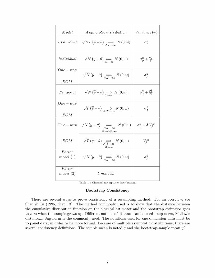
According to Proposition 3, for each panel model speci�cation, convergence of each bootstrap-variance must evaluated. Table 2 presents results for the four panel models. Algebraic details arepresented in appendix 2. Naturally, i.i.d bootstrap is only consistent with i.i.d. panel model.

10

Model Asymptotic distribution V ariance (!) Consistency

I:i:d: panelpNT

�y� � y

� �=)

NT!1N (0; !) �2" Y es

IndividualpNT

�y� � y

� �=)N!1

N (0; !) �2� + �2"

One� way No

ECMpNT

�y� � y

� �=)

N;T!1N (0; !) �2� + �

2"

TemporalpNT

�y� � y

� �=)T!1

N (0; !) �2f + �2"

One� way No

ECMpNT

�y� � y

� �=)

N;T!1N (0; !) �2f + �

2"

Two� waypNT

�y� � y

� �=)

N;T!1N (0; !) �2� + �

2f + �

2" No

ECM

Factor model (1)pNT

�y� � y

� �=)

N;T!1N (0; !) �2� + �

2��

2F + �

2" No

Table 2 : Asymptotic distributions with i.i.d. bootstrap

Individual Bootstrap

In a conceptual manner, individual bootstrap can be perceived as equivalent to i.i.d. bootstrapon fy1:; y2:; :::::yN:g where yi: is intertemporal average for cross-sectional unit i. Equality (4.10)allows to analyze the impact of individual bootstrap with the general speci�cation (2.1, 2.2).�

y�ind � y

�= (��iid � �) +

���iidF � �F

�+�["inter]

�iid � "

�(4.10 )

In a mimic analysis, individual bootstrap does not take care of random process in temporaldimension : the centering drop fftg and fFtg is treated as a constant. This resampling methodis appropriate for f�ig and f�ig. The impact on f"itg seems ambiguous at �rst view. Underassumption A5, intertemporal averages are i.i.d., thus there is a hope. Proposition 4 allows to bemore formal.

Proposition 4 : CLT for individual bootstrapAssume that V ar� (y�i:)

a:s:!N!1

!; then :

pN�y�ind � y

� �=)N!1

N (0; !) (4.11 )

Proof . Apply Proposition 2 to fy1:; y2:; :::::yN:g.

11

Table 3 presents asymptotic distribution for each panel. See details in appendix 3.

Model Asymptotic distribution V ariance (!) Consistency

I:i:d:pNT

�y� � y

� �=)N!1

N (0; !) �2"

Y es

panelpNT

�y� � y

� �=)

N;T!1N (0; !) �2"

IndividualpN�y� � y

� �=)

N;T!1N (0; !) �2� +

�2"T

One� wayY es

ECMpN�y� � y

� �=)

N;T!1N (0; !) �2�

TemporalpN�y� � y

� �=)N!1

N (0; !) �2"

One� way No

ECMpN�y� � y

� �=)

N;T!1N (0; !) �2"

Two� waypN�y� � y

� �=)N!1

N (0; !) �2� +�2"T

No

ECMpN�y� � y

� �=)

N;T!1N (0; !) �2�

FactorpN�y� � y

� �=)

N;T!1N (0; !) �2� Y es

model (1)Table 3 : Asymptotic distributions with individual bootstrap

The guess about f"itg is true. Individual bootstrap is consistent for iid panel model, one-wayECM and factor model. Bootstrap consistency requires N to go to in�nity because resampling isonly in this dimension. There is something sequential in the analysis when N and T go to in�nity.Convergence is given with �xed T �rstly and secondly T goes to in�nity. Equivalence conditionbetwen sequential and joint limit in bootstrap context is to be developed.

12

Temporal Bootstrap

Heuristically, temporal resampling is equivalent to i.i.d bootstrap on fy:1; y:2; :::::y:T g where y:tis cross-sectional average for period t. Equality (4.12) allows to analyze the impact of individualbootstrap with the general speci�cation (2.2).

�y�temp � y

�=�f�iid � f

�+��F

�iid � �F

�+�["cross]

�iid � "

�(4.12 )

Temporal boostrap DGP does not take care of random process in cross-sectional dimension. Ina mimic analysis, this resampling method is appropriate for fftg only if this process is iid. Withf"itg the situation is similar to individual bootstrap case. Proposition 5 permits to be more formal.

Proposition 5 : CLT for temporal bootstrapAssume that V ar� (y�:t)

a:s:!T!1

!; then :

pT�y�temp � y

� �=)T!1

N (0; !) (4.13 )

Proof . Apply Proposition 2 to fy:1; y:2; :::::; y:T g.

Table 4 presents asymptotic distribution for each model. For details, see appendix 4. Temporalbootstrap is consistent with i.i.d. panel model and temporal one-way ECM under i.i.d. assumptionfor fftg. The remark about sequential limit in individual bootstrap case, holds also here.

Model Asymptotic distribution V ariance (!) Consistency

I:i:d:pNT

�y� � y

� �=)T!1

N (0; !) �2"

Y es

panelpNT

�y� � y

� �=)

N;T!1N (0; !) �2"

IndividualpT�y� � y

� �=)T!1

N (0; !) �2"

One� way No

ECMpT�y� � y

� �=)

N;T!1N (0; !) �2"

13

TemporalpT�y� � y

� �=)T!1

N (0; !) �2f +�2"T

One� way Y es if ft is iid

ECMpT�y� � y

� �=)

N;T!1N (0; !) �2f

Two� waypT�y� � y

� �=)T!1

N (0; !) �2f +�2"N

No

ECMpT�y� � y

� �=)

N;T!1N (0; !) �2f

FactorpT�y� � y

� m:s:�!N;T!1

0 No

model (1)Table 4 : Asymptotic distributions with temporal bootstrap

Block Bootstrap

Conceptually, block bootstrap is equivalent to i.i.d. bootstrap on�ybl:1; y

bl:2; :::::y

bl:K

where

ybl:k =1

lN

NXi=1

klXt=kl�k+1

yit

Equality (4.14) presents the impact of block bootstrap with the general speci�cation (2.1-2).�y�bl � y

�=�f�bl � f

�+��F

�bl � �F

�+�"�bl � "

�(4.14 )

Block boostrap DGP does not take care of random process in individual dimension. In a mimicanalysis, it can be said that this resampling method is appropriate for fftg, fFtg and f"itg :

Proposition 6Under assumption A2 and l�1 + lT�1 = o (1) as T !1

pT�f�bl

��=)T!1

N�0; V1f

�(4.15 )

Proof . Under assumption A2 and the convergence rate imposed to l, a demonstration of theconsistency of block bootstrap for time series, can be seen for example in Lahiri (2003), p. 55 .

The condition about the convergence of l has a heuristic interpretation. If l is bounded, theblock bootstrap method fail to capture the real dependence among the data. In other side, if l goesto in�nity at the same rate that T, there are not enough blocks to resample. Block bootstrap isconsistent with i.i.d. panel model and temporal one-way ECM.

14

Model Asymptotic distribution V ariance (!) Consistency

I:i:d:pNT

�y� � y

� �=)T!1

N (0; !) �2"

Y es

panelpNT

�y� � y

� �=)

N;T!1N (0; !) �2"

IndividualpT�y� � y

� �=)T!1

N (0; !) �2"

One� way No

ECMpT�y� � y

� �=)

N;T!1N (0; !) �2"

TemporalpT�y� � y

� �=)T!1

N (0; !) V1f + �2"T

One� way Y es

ECMpT�y� � y

� �=)

N;T!1N (0; !) V1f

Two� waypT�y� � y

� �=)T!1

N (0; !) V1f + �2"N

No

ECMpT�y� � y

� �=)

N;T!1N (0; !) V1f

FactorpT�y� � y

� m:s:�!N;T!1

0 No

model (1)Table 5 : Asymptotic distributions with block bootstrap

Double Resampling Bootstrap

Two schemes of double resampling double bootstrap are explored. In a conceptual manner ,the second scheme can be viewed as an application of �rst scheme, not directly on original data,but on a transformed matrix Y bl that is obtained and by average of periods in each block.

Y bl =nyblik

ok=1;:::;Ki=1;:::;N

with yblik =1

l

klXt=kl�k+1

yit

In the following, the �rst scheme properties are given. Similar results can be easily deduced forthe second scheme. Like in i.i.d bootstrap case, y��it can take any of the NT values of elements of Y;with probability 1=NT: E�� () and V ar�� () are respectively expectation and variance conditionallyon Y , with respect of the double resampling method.

15

E�� (y��it ) = E� (y�it) (4.16)

V ar�� (y��it ) = V ar� (y�it) (4.17)

Expectation and variance are identical to those obtained with i.i.d. bootstrap. The di¤erence isthat conditionally on Y; elements of Y �� are not all independent. Each element has a link with allthe elements in the same column or on the same line with it. This link exists because elements inthe same line belong to the same unit i and elements in the same column refer to the same periodt.

Proposition 7 : Double resampling bootstrap variance8 N;T; the double resampling bootstrap-variance is greater or equal to iid bootstrap-variance :

V ar���y��� � V ar� �y�� (4.18 )

Proof . An analysis of variance gives :

V ar���y���

=1

NTV ar�� (y��it ) +

1

(NT )2

NX(i;t) 6=

TX(j;s)

Cov���y��it ; y

��js

�For i 6= j and t 6= s, Cov��

�y��it ; y

��js

�= 0

For i 6= j; Cov���y��it ; y

��jt

�= V ar� (y�:t) , for t 6= s; Cov�� (y��it ; y��is ) = V ar� (y�i:)

then

V ar���y���

= V ar��y��+

�1� 1

T

�V ar� (y�i:)

N+

�1� 1

N

�V ar� (y�:t)

T

the result follows.

It is important to mention two things about inequality (4.18). Firstly, no particular assumptionshave been made about fy�itg. Secondly, (4.18) is a �nite sample property : it holds for any samplesize. The equality holds in (4.18) when T = 1 (cross-section data) ; N = 1 (time series), or[V ar� (y�i:) ; V ar

� (y�:t)] = (0; 0) ( in cross-sectional averages and temporal averages are constant).Equalities (4.19) and (4.19) permits to analyze the impact of double resampling bootstrap with

the general speci�cation (2.1, 2.2)�y�� � y

�= (��iid � �) +

�f�iid � f

�+���iidF

�iid � �F

�+�"�� � "

�(4.19 )

�y��bl � y

�= (��iid � �) +

�f�bl � f

�+���iidF

�bl � �F

�+�"��bl � "

�(4.20 )

The �rst schme is equivalent to i.i.d. resampling on f�ig ; fftg ; fFtg ; f�ig and �rst schemedouble resampling on f"itg. The second scheme is equivalent to i.i.d. resampling on f�ig ; f�ig blockresampling on fftg ; fFtg and second scheme double resampling on f"itg. It is important to quotethat the second scheme mimics very well the behaviour of f�iFtg : This will permit applicationswith dynamic factors models. At this point, impact of double resampling is known for all processesexcept f"itg : Then, it is important to take care of the distribution of "��. The next propositionconsiders its asymptotic variance with the appropriate scaling factor.

16

Proposition 8 : Double resampling bootstrap-variance for iid observations.Under assumption A4 :

V ar���pNT "

���

a:s:!N;T!1

3.�2" (4.21 )

Proof . Variance decomposition in the proof of Proposition 7 gives

V ar���pNT "

���= V ar� ("�it) +

�1� 1

T

�[T:V ar� ("�i:)] +

�1� 1

N

�[N:V ar� ("�:t)]

V ar� ("�it)a:s:!

NT!1�2" ; [T:V ar

� ("�i:)]a:s:!N!1

�2" ; [N:V ar� ("�:t)]

a:s:!T!1

�2"

then

V ar���pNT "

���

a:s:!N;T!1

3:�2"

Double resampling induces bootstrap-variance three times larger. This may imply a con�denceinterval, larger than the appropriate in case of normality. The question is whether properties offy��it gi;t2N provide asymptotic normality. The next proposition considers with this issue.

Proposition 9 : NormalityUnder assumption A4, , conditionally on Y ,

pNT "

�� converges in distribution to a normallaw.

Proof . See Appendix 7.

Tables 7 and 8 present asymptotic distribution for each panel model. For details about conver-gence, see appendix 6. The result for i.i.d. panel model is due to Proposition 8 and 9. In pratice,if there is a doubt about existence of a dependence in temporal dimension, the best choice is to usethe second scheme.

Why does double resampling work well ?The fact to resample in one dimension has an immediate drawback : processes that are not

in the resampling dimension are dropped out by the centering�y� � y

�. The resampling in two

dimensions avoids this drawback.

17

Model Asymptotic distribution V ariance (!) Consistency

I:i:d: panelpNT

�y�� � y

� �=)

N;T!1N (0; !) 3 �2" Conservative

Individual

One� waypN�y�� � y

� �=)

N;T!1N (0; !) �2� Y es

ECM

Temporal

One� waypT�y�� � y

� �=)

N;T!1N (0; !) �2f Y es if ft is iid

ECM

Two� waypN�y�� � y

� �=)

N;T!1NT!�2[0;1)

N (0; !) �2� + �:�2f

Y es if ft is iid

ECMpT�y�� � y

� �=)

N;T!1NT!1

N (0; !) �2f

FactorpN�y�� � y

� �=)

N;T!1N (0; !) �2� Y es

model (1)Table 6 : Asymptotic distributions with double resampling bootstrap : scheme 1

Model Asymptotic distribution V ariance (!) Consistency

I:i:d: panelpNT

�y�� � y

� �=)

N;T!1N (0; !) 3 �2" Conservative

Individual

One� waypN�y�� � y

� �=)

N;T!1N (0; !) �2� Y es

ECM

Temporal

One� waypT�y�� � y

� �=)

N;T!1N (0; !) V1f Y es

ECM

Two� waypN�y�� � y

� �=)

N;T!1NT!�2[0;1)

N (0; !) �2� + �:V1f

Y es

ECMpT�y�� � y

� �=)

N;T!1NT!1

N (0; !) V1f

FactorpN�y�� � y

� �=)

N;T!1N (0; !) �2� Y es

model (1)Table 7 : Asymptotic distributions with double resampling bootstrap : scheme 2.

18

5 Simulations

This section presents simulation design and results in order to con�rm theorical results. Data Gen-erating Process is the following : � = 0, �i � i:i:d:N (0; 1) , �i � i:i:d: N (0; 1) ; "it � i:i:d:N (0; 1) ;ft and Ft follow the same process an AR (1) : Ft = �Ft�1+�t, �t � i:i:d:N

�0;�1� �2

��with � = 0

or � = 0:5. For each bootstrap resampling scheme, B is equal to 999 replications and the numberof simulations is 1000. Six sample sizes are considered : (N;T ) = (20; 20) ; (30; 30) ; (60; 60) ;(100; 100) ; (60; 10) and (10; 60). For block bootstrap, the block length is l = 5 when T = 100 andl = 2 for other sizes. Tables 8 gives rejection rates with theoretical level 5%.

Simulations con�rm theoretical results. I.i.d bootstrap, individual and temporal bootstrap givegood results for i.i.d panel model. Individual bootstrap performs well with one-way ECM andfactor model. Block bootstrap performs well with i.i.d. model and temporal one-way ECM. Doubleresampling performs well for individual and temporal one-way ECM, two-way ECM and factormodel. Double resampling is conservative for i.i.d. panel model because it induces bootstrap-variance three times larger. In agreement with Proposition 7, under normality, the rejection ratewith double resampling is always smaller than the one observed with i.i.d. resampling, for allsample sizes and all speci�cations. It would be useful to compare simulation results with classicalasymptotical results. For this, a non parametric covariance matrix estimator is needed. Driscoll &Kraay (1998) extends Newey & West (1987)�s covariance matrix estimator to spatially dependentpanel data when N is �xed and T goes to in�nity. Non parametric variance estimation for largepanels is to be developed.

6 Conclusion

This paper considers the issue of bootstrap resampling for panel data. Four speci�cations of paneldata have been considered, namely i.i.d. panel data, one-way error component model, two-way errorcomponent model and lastly factor model. Five bootstrap resampling methods are explored andtheoretical results are presented for the sample mean. It is demonstrated that simple resamplingmethods (i.i.d., individual only or temporal only) are not valid in simple cases of interest, whiledouble resampling that combines resampling in both individual and temporal dimensions is validin these situations. Simulations con�rm these results. The logical follow-up of this paper is toextend results to more complicated statistics. Future research will extend theoretical results tolinear regression model. Resampling methods which are not valid with the sample mean, are ofcourse not valid for general linear regression model, because a mean can be perceived as a specialcase of linear regression.

19

Models (N;T) I.i.d. Ind. Temp. Block 2Res-1 2Res-2

I:i:d: (20;20) 0.042 0.052 0.061 0.096 0.003 0.002(30;30) 0.050 0.067 0.068 0.062 0.001 0.002

panel (60;60) 0.046 0.053 0.053 0.074 0.001 0.001(100;100) 0.052 0.053 0.051 0.104 0.002 0.004

model (60;10) 0.050 0.055 0.103 0.161 0.002 0.002(10;60) 0.052 0.098 0.056 0.067 0.003 0.006

(20;20) 0.563 0.059 0.689 0.714 0.043 0.040Individual (30;30) 0.621 0.051 0.724 0.742 0.041 0.039

(60;60) 0.743 0.059 0.810 0.842 0.050 0.048One� way (100;100) 0.782 0.061 0.852 0.843 0.054 0.049

(60;10) 0.391 0.054 0.591 0.650 0.040 0.038ECM (10;60) 0.725 0.091 0.817 0.826 0.082 0.050

(20;20) 0.736 0.822 0.299 0.090 0.268 0.068Temporal (30;30) 0.762 0.835 0.255 0.067 0.236 0.053

(60;60) 0.813 0.870 0.263 0.063 0.253 0.054One� way (100;100) 0.886 0.919 0.268 0.062 0.268 0.054ECM (60;10) 0.841 0.880 0.304 0.146 0.299 0.132(� = 0:5) (10;60) 0.621 0.750 0.244 0.066 0.215 0.040

(20;20) 0.581 0.164 0.158 0.216 0.041 0.048Two� way (30;30) 0.663 0.166 0.158 0.178 0.048 0.056

(60;60) 0.743 0.177 0.176 0.186 0.042 0.048ECM (100;100) 0.830 0.161 0.174 0.190 0.053 0.047

(60;10) 0.692 0.449 0.125 0.164 0.090 0.090� = 0 (10;60) 0.680 0.110 0.431 0.060 0.077 0.430

(20;20) 0.687 0.327 0.355 0.203 0.140 0.042Two� way (30;30) 0.767 0.324 0.342 0.194 0.143 0.051

(60;60) 0.837 0.328 0.329 0.202 0.159 0.047ECM (100;100) 0.872 0.360 0.355 0.185 0.168 0.051

(60;10) 0.781 0.600 0.297 0.152 0.226 0.094� = 0:5 (10;60) 0.733 0.161 0.491 0.418 0.096 0.050

(20;20) 0.4830 0.056 0.625 0.598 0.034 0.024Factor (30;30) 0.524 0.062 0.644 0.644 0.044 0.039model (60;60) 0.677 0.063 0.747 0.764 0.053 0.054(1) (100;100) 0.755 0.057 0.823 0.818 0.048 0.056

(60;10) 0.364 0.067 0.543 0.508 0.033 0.020(10;60) 0.692 0.096 0.756 0.754 0.081 0.064(20;20) 0.119 0.086 0.173 0.176 0.002 0.002

Factor (30;30) 0.121 0.067 0.158 0.034 0.002 0.002model (60;60) 0.140 0.063 0.163 0.098 0.003 0.002(2) (100;100) 0.120 0.049 0.118 0.104 0.001 0.001

(60;10) 0.116 0.067 0.194 0.282 0.002 0.004(10;60) 0.133 0.112 0.151 0.068 0.007 0.002

Table 8 : Simulation results

20

References

[1] Andersson M. K. & Karlsson S. (2001) Bootstrapping Error Component Models, ComputationalStatistics, Vol. 16, No. 2, 221-231.

[2] Anselin L. (1988) Spatial Econometrics: Methods and Models, Kluwer Academic Publishers,Dordrecht.

[3] Bai J. & Ng S. (2004) A Panic attack on unit roots and cointegration, Econometrica, Vol. 72,No 4, 1127-1177.

[4] Balestra P. & Nerlove M. (1966) Pooling Cross Section and Time Series data in the estimationof a Dynamic Model : The Demand for Natural Gas, Econometrica, Vol. 34, No 3, 585-612.

[5] Baltagi B. (1995) Econometrics Analysis of Panel Data, John Wiley & Sons.

[6] Bellman L., Breitung J. & Wagner J. (1989) Bias Correction and Bootstrapping of ErrorComponent Models for Panel Data : Theory and Applications, Empirical Economics, Vol. 14,329-342.

[7] Beran R. (1988) Prepivoting test statistics: a bootstrap view of asymptotic re�nements, Journalof the American Statistical Association, Vol. 83, No 403, 687�697.

[8] Bickel P. J. & Freedman D. A. (1981) Some Asymptotic Theory for the Bootstrap, The Annalsof Statistics, Vol. 9, No 6, 1196-1217.

[9] Carvajal A. (2000) BC Bootstrap Con�dence Intervals for Random E¤ects Panel Data Models,Working Paper Brown University, Department of Economics.

[10] Davidson R. (2007) Bootstrapping Econometric Models, This paper has appeared, translatedinto Russian, in Quantile, Vol. 3, 13-36.

[11] Driscoll J. C. & . Kraay A. C. (1998) Consistent Covariance Matrix Estimation with SpatiallyDependent Panel Data, The Review of Economics and Statistics, Vol. 80, No 4 , 549�560.

[12] Efron B. (1979) Bootstrap Methods : Another Look at the Jackknife, The Annals of Statistics,Vol. 7, No 1, 1-26.

[13] Everaert G. & Pozzi L. (2007) Bootstrap-Based Bias Correction for Dynamic Panels, Journalof Economic Dynamics & Control, Vol. 31, 1160-1184.

[14] Focarelli D. (2005) Bootstrap bias-correction procedure in estimating long-run relationshipsfrom dynamic panels, with an application to money demand in the euro area, Economic Mod-elling, Vol. 22, 305�325.

[15] Freedman D.A. (1981) Bootstrapping Regression Models, The Annals of Statistics, Vol. 9, No6, 1218-1228.

[16] Fuller W. A. & Battese G. E. (1974) Estimation of linear models with crossed-error structure,Journal of Econometrics, Vol. 2, No 1, 67-78.

[17] Herwartz H. (2007) Testing for random e¤ects in panel models with spatially correlated distur-bances, Statistica Neerlandica, Vol. 61, No 4, 466�487.

21

[18] Herwartz H. (2006) Testing for random e¤ects in panel data under cross-sectional error corre-lation �a bootstrap approach to the Breusch Pagan Test, Computational Statistics and DataAnalysis, Vol. 50, 3567�3591.

[19] Hsiao C. (2003) Analysis of Panel Data, 2nd Edition. Cambridge University Press.

[20] Ibragimov I.A. (1962) Some limit theorems for stationary processes, Theory of Probability andIts Applications Vol. 7, 349�382.

[21] Kapetanios G. (2004) A bootstrap procedure for panel datasets with many cross-sectional units,Working Paper No. 523, Department of Economics, Queen Mary, London. Forthcoming inEconometrics Journal.

[22] Künsch H. R. (1989) The jackknife and the bootstrap for general stationary observations, An-nals of Statistics, Vol. 17, 1217�1241.

[23] Lahiri S. N. (2003) Resampling Methods for Dependent Data, Springer Series in Statistics,Sinpring-Verlag, New York.

[24] Liu R. Y. (1988) Bootstrap Procedure Under Nome Non-i.i.d. Models, Annals of Statistics, Vol.16, 1696�1708.

[25] Liu R. Y. & Singh K. (1992) Moving Block Jackknife and bootstrap capture weak dependence,in Exploring the Limits of Bootstrap , eds, by Lepage and Billard, John Wiley, NewYork.

[26] Moon H. R. & Perron B. (2004) Testing for unit root in panels with dynamic factors, Journalof Econometrics, Vol. 122, 81-126.

[27] Mundlak Y. (1978) On the Pooling of Time Series and Cross Section Data, Econometrica,Vol. 46, 1, 69-85.

[28] Newey W. K. & West K. D. (1987) A Simple, Positive Semi-De�nite, Heteroskedasticity andAutocorrelation Consistent Covariance Matrix, Econometrica, Vol. 55, No 3, 703-708.

[29] Phillips P.C.B. & Sul D. (2003) Dynamic panel estimation and homogeneity testing undercross-section dependence, Econometrics Journal, Vol. 6, 217-259.

[30] Phillips P.C.B. & Moon H.R. (1999) Linear Regression Limit Theory for Nonstationary PanelData, Econometrica, Vol. 67, No 5, 1057-1112.

[31] Politis D. & Romano J. (1994) The stationary bootstrap, Journal of the American StatisticalAssociation, Vol. 89, 1303-1313.

[32] Politis D. & Romano J. (1992) A circular block resampling procedure for stationary data, inExploring the Limits of Bootstrap eds. by Lepage and Billard, John Wiley, NewYork.

[33] Pólya G. (1920) Uber den zentralen Grenzwertsatz der Wahrscheinlinchkeitsrechnug und Mo-menten problem, Math. Zeitschrift, 8.

[34] Ser�ing R. J. (1980) Approximation Theorems of Mathematical Statistics, New York: Wiley.

[35] Shao J. & Tu D. (1995) The Jackknife and bootstrap, Sinpring-Verlag, New York.

[36] Singh K. (1981) On the Asymptotic Accuracy of Efron�s Bootstrap, The Annals of Statistics,Vol. 9, No. 6, 1187-1195.

22

[37] Wu C. F. J. (1986) Jackknife, bootstrap and other resampling methods in regression analysis,Annals of Statistics, Vol. 14, 1261�1295.

[38] Yang S.S. (1988) A Central Limit Theorem for the Bootstrap Mean, The American Statistician,Vol. 42, 202-203.

7 APPENDIX

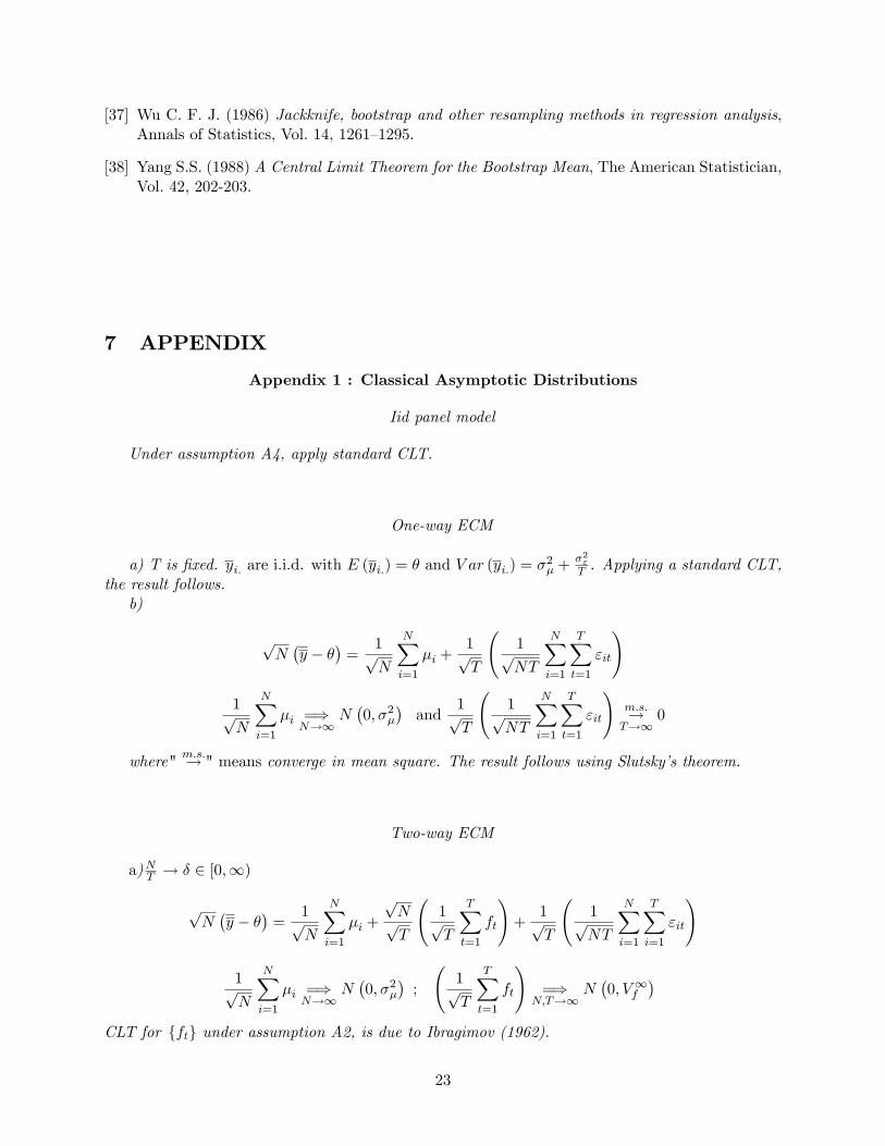
Appendix 1 : Classical Asymptotic Distributions

Iid panel model

Under assumption A4, apply standard CLT.

One-way ECM

a) T is �xed. yi: are i.i.d. with E (yi:) = � and V ar (yi:) = �2� +

�2"T . Applying a standard CLT,

the result follows.b)

pN�y � �

�=

1pN

NXi=1

�i +1pT

1pNT

NXi=1

TXt=1

"it

!

1pN

NXi=1

�i =)N!1

N�0; �2�

�and

1pT

1pNT

NXi=1

TXt=1

"it

!m:s:!T!1

0

where" m:s:! " means converge in mean square. The result follows using Slutsky�s theorem.

Two-way ECM

a)NT ! � 2 [0;1)

pN�y � �

�=

1pN

NXi=1

�i +

pNpT

1pT

TXt=1

ft

!+

1pT

1pNT

NXi=1

TXi=1

"it

!

1pN

NXi=1

�i =)N!1

N�0; �2�

�;

1pT

TXt=1

ft

!=)

N;T!1N�0; V1f

�CLT for fftg under assumption A2, is due to Ibragimov (1962).

23

1pT

1pNT

NXi=1

TXt=1

"it

!m:s:!

N;T!10

The result follows3.b)NT !1

pT�y � �

�=

pTpN

1pN

NXi=1

�i

!+

1pT

TXt=1

ft

!+

1pN

1pNT

NXi=1

TXi=1

"it

!

1pN

1pNT

NXi=1

TXt=1

"it

!m:s:!

N;T!10;

pTpN

1pN

NXi=1

�i

!m:s:!

N;T!10

1pT

TXt=1

ft

!=)T!1

N�0; V1f

�The result follows.

Factor Models

First speci�cation : yit = � + �i + �iFt + "it

pN�y � �

�=

1pN

NXi=1

�i +

1pN

NXi=1

�i

! 1

T

TXt=1

Ft

!+

1pT

1pNT

NXi=1

TXt=1

"it

!

1pT

1pNT

NXi=1

TXt=1

"it

!m:s:!

N;T!10 ;

1pN

NXi=1

�i

! 1

T

TXt=1

Ft

!m:s:!

N;T!10

The result follows.

Second speci�cation : yit = � + �iFt

pNT

�y � �

�=

1pN

NXi=1

�i

! 1pT

TXt=1

Ft

!

1pN

NXi=1

�i ) N�0; �2�

� 1pT

TXt=1

Ft ) N (0; V1F )

To my knowledge, there is no theory about the convergence of the product. For Slutsky theorem,a convergence in probabilty at least, is needed.

3When the vector(Xn; Yn)0converges to a normal distribution, the asymptotic distribution of any linear combina-

tion of the elements of the vector (in particular the sum) can be deduced. The fact that Xn and Yn are independentand converge to a normal distribution, implies that their sum converge to the sum of their asymptotic normaldistributions.

24

Appendix 2 : I.i.d. Bootstrap

V ar� (y�it) !

Iid panel model 1NT

NXi=1

TXt=1

("it)2 �

�"�2 !

NT!1�2"

Ind. 1-way ECM 1NT

NXi=1

TXt=1

(�i + "it)2 �

��+ "

�2 !N!1

�2� + �2" ;

a:s:!N;T!1

�2� + �2"

Temp. 1-way ECM 1NT

NXi=1

TXt=1

(ft + "it)2 �

��+ "

�2 !T!1

�2f + �2" ;

a:s:!N;T!1

�2f + �2"

Two-way ECM 1NT

NXi=1

TXt=1

(�i + ft + "it)2 �

��+ f + "

�2 !N;T!1

�2� + �2f + �

2"

Factor Model (1) 1NT

NXi=1

TXt=1

(�i + �iFt + "it)2 �

��+ �F + "

�2 !N;T!1

�2� + �2� � �2F + �2"

Appendix 3 : Individual Bootstrap

V ar� (yi:) !

Iid panel model 1N

NXi=1

("i:)2 �

�"�2 !

N!1�2"T

Ind. 1-way ECM 1N

NXi=1

(�i + "i:)2 �

��+ "

�2 !N!1

�2� +�2"T ; !

N;T!1�2�

Temp. 1-way ECM 1N

NXi=1

("i:)2 �

�"�2 !

N!1�2"T

Two-way ECM 1N

NXi=1

(�i + "i:)2 �

��+ "

�2 !N!1

�2� +�2"T ; !

N;T!1�2�

Factor Model (1) 1N

NXi=1

��i + �iF + "i:

�2 � ��+ �F + "�2 !N;T!1

�2�

25

Appendix 4 : Temporal Bootstrap

V ar� (y:t) !

Iid panel model 1T

TXt=1

(":t)2 �

�"�2 !

T!1�2"N

Ind. 1-way ECM 1T

TXt=1

(":t:)2 �

�"�2 !

T!1�2"N

Temp. 1-way ECM 1T

TXt=1

(ft + ":t)2 �

�"�2 !

T!1�2f +

�2"N ; !

N;T!1�2f

Two-way ECM 1T

TXt=1

(ft + ":t)2 �

�"�2 !

T!1�2f +

�2"N ; !

N;T!1�2f

Factor Model (1) 1T

TXt=1

��Ft + ":t

�2 � ��F + "�2 m:s:!N;T!1

0

Appendix 5 : Block Bootstrap

V ar��ybl:k�

!

Iid panel model 1K

KXk=1

�"bl:k�2 � �"�2 !

T!1�2"N

Ind. 1-way ECM 1K

KXt=1

�"bl:k�2 � �"�2 !

T!1�2"N

Temp. 1-way ECM 1K

KXk=1

�fbl:k + "

bl:k

�2���+ "

�2 !T!1

V1f + �2"N ; !

N;T!1V1f

Two-way ECM 1K

KXk=1

�fbl:k + "

bl:k

�2���+ "

�2 !T!1

V1f + �2"N ; !

N;T!1V1f

Factor Model (1) 1K

KXk=1

��F

bl:k + "

bl:k

�2���+ �F + "

�2 m:s:!N;T!1

0

26

Appendix 6 : Double Resampling BootstrapI.i.d. panel model

Use Propositions 8 and 9.

One-way ECMpN�y�� � y

�=pN (��iid � �) +

pN�"�� � "

�pN (�� � �) �

=)N!1

N�0; �2�

�;hpN�"�� � "

�i m:s:�!N;T!1

0

The result follows.

Two-way ECM

a) NT ! � 2 [0;1) :

pN�y�� � y

�=pN (�� � �) +

pNpT

pT�f� � f

�+

1pT

hpNT

�"�� � "

�ipNpT

pT�f� � f

��=)

N;T!1N�0; �:�2f

�,

pNpT

pT�f�bl � f

��=)

N;T!1N�0; �:V1f

�1pT

hpNT

�"�� � "

�i m:s:�!N;T!1

0

There result follows.

b) NT !1 :

pT�y�� � y

�=

pTpN

hpN (�� � �)

i+pT�f� � f

�+

pTpN

�1pT

hpNT

�"�� � "

�i�pT�f� � f

��=)T!1

N�0; �2f

� pT�f�bl � f

��=)T!1

N�0; V1f

�1pN

hpNT

�"�� � "

�i m:s:�!N;T!1

0 ,

pTpN

hpN (�� � �)

im:s:�!

N;T!10

The result follows.

Factor ModelpN�y�� � y

�=pN (��iid � �) +

pN���iidF

�iid � �F

�+hpN�"�� � "

�ihpN�"�� � "

�i m:s:�!N;T!1

0 ;pN���iidF

�iid � �F

�m:s:�!

N;T!10

the results follows.

27

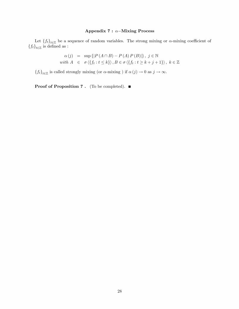
Appendix 7 : ��Mixing Process

Let fftgt2Z be a sequence of random variables. The strong mixing or �-mixing coe¢ cient offftgt2Z is de�ned as :

� (j) = sup fjP (A \B)� P (A)P (B)jg ; j 2 Nwith A 2 � hfft : t � kgi ; B 2 � hfft : t � k + j + 1gi ; k 2 Z

fftgt2Z is called strongly mixing (or �-mixing ) if � (j)! 0 as j !1:

Proof of Proposition 7 . (To be completed).

28