BOOTSTRAP AND APPLICATIONS - crrao AND APPLICATIONS ... Nonparametric Regression + Classification...

1

BOOTSTRAP AND APPLICATIONS A workshop conducted at the CR Rao Advanced Institute of Mathematics, Statistics, and Computer Science, University of Hyderabad January 2-3, 2014 MB Rao University of Cincinnati Outline

1. Introduction to Bootstrap 2. Bootstrap distribution of an estimator 3. Applications in Random Forests, Bagging, and Boosting

The Bootstrap: The essentials Problem A random phenomenon X is under observation. Its distribution is symbolically denoted by F(.), which is unknown. We are interested in some feature θ of the population. Equivalently, θ = θ(F) is a specific property of the distribution. Examples: θ = mean, median, standard deviation, 10th percentile, etc. Example Acute Myelogenous Leukemia is treatable by a combination of radiation and chemotherapy. The success rate of a cure (disease is under remission) is very, very high. Once the patient reaches a well-defined state of remission, medical researchers make every effort to prolong the state of remission. A proposal is made. Administer low doses of chemotherapy on a weekly basis. Is it better than doing nothing? We have to conduct a comparative experiment. Design: Select a random sample of patients. Cases: Some get low doses of chemotherapy weekly. Controls: Do nothing for the others. Randomize the patients into one of the groups. Get funding for a pilot project. The random phenomenon of interest: X = Length of time (in weeks) the disease is under remission until a relapse occurs.

2

X = Time at which relapse occurs. The entity X varies from patient to patient. Let F1 be the distribution of X among the population of cases. Let F2 be the distribution of X among the population of controls. θ1 = Probability that relapse occurs after 2 years under the distribution F1 = S1(2) = 1 – F1(2). θ2 = Probability that relapse occurs after 2 years under the distribution F2 = S2(2) = 1 – F2(2). Goals: Estimate the probabilities of interest using the data collected. Assess their accuracies (standard errors). Provide a 95% confidence interval for the difference θ1 – θ2. Pilot studies involve small sample sizes. Further funding depends on the confidence interval you built. Back to the main problem: A random sample X1, X2, … , Xn from the distribution of F. Let �� = ��(��, �, … , ��) be an estimate of θ. We want to assess its accuracy. It is simply its standard deviation. It is called standard error. Generally, there is no explicit formula for the standard error. Exception: θ = mean of F �� = sample mean SE(��) = σ/sqrt(n) If we can obtain the sampling distribution of ��, we can calculate its standard error, build confidence intervals, etc. What are the options?

1. Derive it. Not always possible. 2. Use asymptotics. The sample size n is small. 3. The distribution F is a member of a parametric family. The estimate is

a likelihood estimate. Use the asymptotic theory of the likelihood estimators. The sample size is still small.

4. Draw random samples of size n from the distribution of F many, many

times. Keep calculating �� for each sample. We will now have a

veritable bank of �� s. Build the sampling distribution empirically. Not practical – expensive.

3

A poor man’s solution: Computing is cheap: Population: X1 X2 … Xn Probability: 1/n 1/n … 1/n The data collected is the population. This is the empirical distribution of the data. It is denoted by �. i-th Bootstrap sample Draw a random sample of size n with replacement from the above distribution �. ��∗ , ��∗ , … , ��∗ Calculate the estimate based on this sample: ��∗� =��(��∗ , ��∗ , … , ��∗ ) i = 1, 2, … , B B is large. Build a histogram of ��∗�s. This is our Bootstrap estimate of the sampling distribution of ��. Rationale F is the underlying distribution. Feature of interest: θ = θ(F) Random sample from F: X1, X2, … , Xn Estimate: �� = ��(��, �, … , ��) Find the distribution of �� under F. A nonparametric maximum likelihood estimate of F is the empirical distribution �. � is the underlying distribution. Feature of interest: θ = θ( �) Random sample from �: ��∗ �∗ … ��∗ (Bootstrap sample) Estimate: �∗� =�∗(� ��∗, �∗, …, ��∗) Find the distribution of �∗�under �. This is what I am doing under the Bootstrap procedure. The empirical distribution �is an estimate of F. The distribution of �∗�under � is an estimate of the distribution of �� under F. When do we use the Bootstrap procedure? A competitor to the bootstrap is the permutation procedure.

4

Number of permutations: n! Number of bootstrap samples: nn It seems as though there are many, many more bootstrap samples. Not really! n = 2 Number of possible distinct bootstrap samples: 3 X1 X1 X2 X2 X1 X2 n = 3 Number of possible distinct bootstrap samples: 10 Think about it! General formula

Number of distinct bootstrap samples: �2� − 1� � = (��)!�!(��)!

Note that 3n-1 ≥ �2� − 1� � ≥ 2n-1 if n ≥ 2.

Which is bigger n! or 3n-1? Duplicated bootstrap samples reduce its reliability.

n = 10: �2� − 1� � = 92,378

If n < 10, the bootstrap may not be reliable. If n = 20 and B = 2000, the chances of obtaining two identical bootstrap samples is < 0.05. Go ahead with the bootstrap! Applications Nonparametric Regression + Classification Trees + ‘rpart’ package

5

If we have a binary response variable and some covariates, we can build a model connecting the binary response variable with the covariates using logistic regression. The logistic regression model is probabilistic in nature. There are a number of other approaches. One approach popular with engineers and physicists is to treat the problem as a pattern recognition or classification problem. Let us look at the abdominal sepsis problem. Response variable Y = 1 if the patient dies after surgery = 0 if the patient survives after surgery Independent variables X1: Is the patient in a state of shock? X2: Is the patient suffering from undernourishment? X3: Is the patient alcoholic? X4: Age X5: Has the patient bowel infarction? In logistic regression, the probability distribution of Y is modeled in terms of the covariates.

Ln ��(��)��(��) = β0 + β1*X 1 + β2*X 2 + β3*X 3 + β4*X 4 + β5*X 5

= Natural logarithm of the odds of Death versus Life I fitted this model to the data. The following is the output. Variable Regression Standard z-value p-value Coefficient Error Intercept -9.754 2.534 - - Shock 3.674 1.162 3.16 0.0016 Malnutrition1.217 0.7274 1.67 0.095 Alcoholism 3.355 0.9797 3.43 0.0006 Age 0.09215 0.03025 3.04 0.0023 Infarction 2.798 1.161 2.41 0.016 Estimated model

6

ln(π

π−1

) = -9.754 + 3.674*X1 + 1.217*X2 + 3.355*X3 + 0.09215*X4 +

2.798*X5 All covariates except ‘Malnutrition’ are significant. A goodness-of-fit test is conducted. The model is an adequate summary of the data. This is a model based approach to the problem. Advantages:

1. One can test whether a predictor Xi has a significant impact on the response variable Y, i.e., test the null hypothesis that βi = 0.

2. One can test the hypothesis whether the model postulated is an adequate summary of the data, i.e., conduct a goodness-of-fit test.

3. One can identify a parsimonious model adequately summarizing the data.

Another approach: empirical: classification tree: If we view this problem as a pattern recognition problem, we need to identify what the patterns are. The situation Y = 1 is regarded as one pattern and Y = 0 as the other. Once we have information on the independent variables for a patient, we need to classify him/her into one of the two patterns. We have to come up with a protocol, which will classify the patient as falling into one of the patterns. In other words, we have to say whether he will die or survive after surgery. We will not make a probability statement. Any classification protocol one comes up cannot be expected to be free of errors. A classification protocol is judged based on its misclassification error rate. We will make precise this concept later. Core idea: Look at the space of predictors. We want to break up the predictor space into boxes (5-dimensional parallelepipeds) so that each box is identified with one pattern. For example, Shock = 1, Malnourishment = 0, Alcoholism = 1, Age > 45, Infarction = 1 is one such box. Can we say that most of the patients that fall into this box die? We want to divide the predictor space into mutually exclusive and exhaustive boxes so that the patients falling into each box have predominantly one pattern, either death or

7

life. The creation of such boxes is the main objective of the current endeavor. More simplistically, we should be able to make statements like: Aha! If X1 ≤ 0.5, X2 > 0.5, X3 < 0.5, X4 < 50, and X5 > 0.5, most patients die! One popular method in classification or pattern recognition is the so called the ‘classification tree methodology,’ which is a data mining method. The methodology was first proposed by Breiman, Friedman, Olshen, and Stone in their monograph published in 1984. This goes by the acronym CART (Classification and Regression Trees). A commercial program called CART can be purchased from Salford Systems. Other more standard statistical software such as SPLUS, SPSS, SAS, MATLAB, and R also provide tree construction procedures with user-friendly graphical interface. The packages ‘rpart,’ ‘tree,’ and ‘party’ do classification trees. Some of the material I am presenting in this presentation is culled from the following two books. L Breiman, J H Friedman, R A Olshen, and C J Stone – Classification and Regression Trees, Wadsworth International Group, 1984. Heping Zhang and Burton Singer – Recursive Partitioning in the Health Sciences, Second Edition, Springer, 2008. Various computer programs related to this methodology can be downloaded freely from Heping Zhang’s web site: http://peace.med.yale.edu/pub Basic ideas in the development of a classification tree Let me work with an artificial example: One binary response variable Y and two quantitative variables X1 and X2. ID Y X1 X2

1 0 1 2 2 1 6 5 3 1 5 7 4 0 10 9 5 0 5 5 6 1 4 8 7 1 10 2

8

8 0 4 3 9 1 8 4 10 0 9 7 11 1 3 9 12 0 8 8 13 1 9 2 14 0 3 1 15 0 7 7 16 1 2 10 17 0 6 10 18 1 7 5 19 1 1 6 20 0 2 4 Goal: I know one with given X1 and X2 values. I need to classify him as having the pattern Y = 0 or Y = 1. We have the training data given above to develop a classification protocol. (I could have done a logistic regression here.) Another view point: What ranges of X1 and X2 values identify the pattern {Y = 0} mostly and what for the pattern {Y = 1} mostly? I am going to build a tree with my bare hands. Step 1: Put all the subjects into the root node. There are 10 subjects with the pattern Y = 0 and ten with Y = 1. Step 2: Let us split the mother node into two daughter nodes. We need to choose one of the covariates. Let us choose X1. We need to choose one of the numbers taken by X1. The possible values of X1 are 1, 2, … , 10. Let us choose 5. All those subjects with X1 ≤ 5 go into the left daughter node. All those subjects with X1 > 5 go into the right daughter node. Members of the left daughter node: ID 1, 3, 5, 6, 8, 11, 14, 16, 19, 20. Five of these subjects have the pattern {Y = 0} and the rest {Y = 1}. Members of the right daughter node: ID 2, 4, 7, 9, 10, 12, 13, 15, 17, 18. Five of these subjects have the pattern {Y = 0} and the rest {Y = 1}.

9

Step 3. Let us split the left daughter node. Choose one of the covariates. Let us choose now X2. Let us choose one of the numbers taken by X2. Let us choose 5. Shepherd all those subjects with X2 ≤ 5 into the left grand daughter node and those with X2 > 5 into the right grand daughter node. Composition of the subjects in the left granddaughter node: ID 1, 5, 8, 14, 20. All these subjects have the pattern {Y = 0}. This granddaughter is the purest. There is no need to split the granddaughter. This is a terminal node. Declare this node as {Y = 0} node. Composition of the subjects in the right granddaughter node: ID 3, 6, 11, 16, 19. All these subjects have the pattern {Y = 1}. This granddaughter is the purest. There is no need to split the granddaughter. This is a terminal node. Declare this node as {Y = 1} node. Step 4. Let us split the right daughter node. Choose one of the covariates. Let us choose X2. Let us choose one of the numbers taken by X2. Let us choose 5. Shepherd all those subjects with X2 ≤ 5 into the left grand daughter node and those with X2 > 5 into the right grand daughter node. Composition of the subjects in the left granddaughter node: ID 2, 7, 9, 13, 18. All these subjects have the pattern {Y = 1}. This granddaughter is the purest. This is a terminal node. Declare this node as {Y = 1} node. Composition of the subjects in the right granddaughter node: ID 4, 10, 12, 15, 17. All these subjects have the pattern {Y = 0}. This granddaughter is the purest. This is a terminal node. Declare this node as {Y = 0} node. The task of building a tree is complete. Look at the tree that results. Let us now calculate the misclassification error rate. Let us pour all the subjects into the mother node. We know the pattern each subject has. Check which terminal node they fall into. Check whether its true pattern matches with the pattern of the terminal node. The percentage of mismatches is the misclassification rate. Misclassification rate = 0%. How does one use this classification protocol in practice? Take a subject whose pattern is unknown. We have its covariate values. Pour this subject

10

into the mother node. See where he lands. Note the identity of the terminal node. That is the pattern he is classified into. I built the tree with my bare hands. This tree can also be drawn in a different way. We use the ‘polygon’ command of R. First, present a verbal description of the tree I built. If X 1 ≤ 5 and X2 ≤ 5, classify the subject to have the pattern {Y = 0}. If X 1 ≤ 5 and X2 ≥ 6, classify the subject to have the pattern {Y = 1}. If X 1 ≥ 6 and X2 ≤ 5, classify the subject to have the pattern {Y = 1}. If X 1 ≥ 5 and X2 ≥ 6, classify the subject to have the pattern {Y = 0}. The statement X1 ≤ 5 and X2 ≤ 5 is equivalent to, graphically, the rectangle with vertices (1, 1), (1, 5), (5, 5), (5, 1) in the X1 – X2 plane. The command ‘polygon’ draws the rectangle. First, we need to create a blank plot setting the X1- and X2-axes. The input type = “n” exhorts the plot that there should be no points imprinted on the graph. > plot(c(1,10), c(1, 10), type = "n", xlab = "X1", ylab = "X2", main = "Classification Protocol") The ‘polygon’ command has essentially two major inputs. The x-input should have all the x coordinates of the points. The y-input should have all the corresponding y-coordinates of the points. The polygon thus created latches onto the existing plot. > polygon(c(1, 1, 5, 5), c(1, 5, 5, 1), col = "gray", border = "blue", lwd = 2) The statement X1 ≤ 5 and X2 ≥ 6 is equivalent to, graphically, the rectangle with vertices (1, 6), (1,10), (5, 10), (5, 6) in the X1 – X2 plane. > polygon(c(1, 1, 5, 5), c(6, 10, 10,6), col = "yellow", border = "blue", lwd = 2) The other polygons are created in the same way. > polygon(c(6, 6, 10, 10), c(6, 10, 10,6), col = "mistyrose", border = "blue", lwd = 2) > polygon(c(6, 6, 10, 10), c(1, 5, 5, 1), col = "cyan", border = "blue", lwd = 2)

11

We need to identify each rectangle with a pattern. The text command needs the coordinates (x-coordinate and y-coordinate) at which the legend is to be implanted. The coordinates are to be followed by the legend in double quotes. The color is optional. The default is ‘black.’ > text(3, 3, "{Y = 0}", col = "red") > text(3, 8, "{Y = 1}", col = "blue") > text(8, 8, "{Y = 0}", col = "red") > text(8, 3, "{Y = 1}", col = "blue") The following is a graphical presentation of the classification tree.

2 4 6 8 10

24

68

10

Classification Protocol

X1

X2

{Y = 0}

{Y = 1} {Y = 0}

{Y = 1}

12

Questions

1. Which variable one should choose to split a node? 2. Once the variable is chosen, what cut-point is to be chosen to create

daughter nodes? We use entropy to guide our choices. Suppose we have a random variable X taking finitely many values with some probability distribution. X: 1 2 … m Pr.: p1 p2 … pm We want to measure the degree of uncertainty in the distribution (p1, p2, … , pm). For example, suppose m = 2. Look at the distributions (1/2, 1/2) and (0.99, 0.01). There is more uncertainty in the first distribution than in the second. Suppose someone is about to crank out or simulate X. I am more comfortable in betting on the outcome of X if the underlying distribution is (0.99, 0.01) than when the distribution is (1/2,1/2). We want to assign a numerical quantity to measure the degree of uncertainty. Entropy of a distribution is introduced as a measure of uncertainty.

Entropy (p1, p2, … , pm) = ∑=

−m

iii pp

1ln = Entropy impurity = Measure of

Chaos, with the convention that 0 ln 0 = 0. Properties

1. 0 ≤ Entropy ≤ ln m. 2. The minimum 0 is attained for each of the distributions (1, 0, 0, … ,

0), (0, 1, 0, … , 0), … , (0, 0, … , 0, 1). For each of these distributions, there is no uncertainty. The entropy is zero.

3. The maximum ln m is attained at the distribution (1/m, 1/m, … , 1/m). The uniform distribution is the most chaotic. Under this uniform distribution, uncertainty is maximum.

There are other measures of uncertainty available in the literature.

13

Gini’s measure of uncertainty for the distribution (p1, p2, … , pm) = ∑≠ ji

ji pp .

Properties 1. 0 ≤ Gini’s measure ≤ (m-1)/m. 2. The minimum 0 is attained for each of the distributions (1, 0, 0, … ,

0), (0, 1, 0, … , 0), … , (0, 0, … , 0, 1). For each of these distributions, there is no uncertainty. The Gini’s measure is zero.

3. The maximum (m-1)/m is attained at the most chaotic distribution (1/m, 1/m, … , 1/m). Under this uniform distribution, the uncertainty is maximum.

Another measure of uncertainty is defined by min {p1, p2, … , pm}. How entropy is used to pick up a covariate for splitting the mother node? Discuss. Take a node. We want to split it into two sub-nodes. Take a covariate X4 (Age), say. Take a cut-point 40, say. Shepherd all patients with Age ≤ 40 into the left sub-node. Determine the distribution of Death and Life within the sub-node. Calculate its entropy. Shepherd all patients with Age > 40 into the right sub-node. Determine the distribution of Death and Life with in the sub-node. Calculate its entropy. We want the distributions in the sub-nodes less chaotic than the distribution of the mother node. Compare the mother with the daughters collectively. Calculate weighted entropy of the daughters. Daughters’ entropy = Weight of the left sub-node*Its entropy + Weight of the right sub-node*Its entropy Minimize daughters’ entropy! With respect to what? Why? Computations Terry Therneau and Elizabeth Atkinson (Mayo Foundation) have developed ‘rpart’ (recursive partitioning) package to implement classification trees and regression trees in all their glory. The method depends what kind of response variable we have. Categorical → method = “class” Continuous → method = “anova” Count → method = “poisson”

14

Survival → method = “exp” They have two monographs on their package available on the internet. An introduction to Recursive Partitioning using the RPART routines, February, 2000 Same title, September, 1997 Both are very informative. Let me illustrate ‘rpart’ command in the context of a binary classification problem. Four data sets are available in the package. Download ‘rpart.’

� data(package = “rpart”) Data sets in the package ‘rpart’: car.test.frame Automobile Data from 'Consumer Reports' 1990 cu.summary Automobile Data from ‘Consumer Reports' 1990 kyphosis Data on Children who have had Corrective Spinal Surgery solder Soldering of Components on Printed-Circuit Boards Let us look at ‘kyphosis’ data. > data(kyphosis) > dim(kyphosis) [1] 81 4 > head(kyphosis) Kyphosis Age Number Start 1 absent 71 3 5 2 absent 158 3 14 3 present 128 4 5 4 absent 2 5 1 5 absent 1 4 15 6 absent 1 2 16 Look at the documentation on the data.

15

Look at the documentation on ‘rpart.’ If we let the partition continue without any break, we will end up with a saturated tree. Every terminal node is pure. It is quite possible some terminal nodes contain only one data point. One has to declare each terminal node as one of the two types: present or absent. Majority rules. Discuss We need to arrest the growth of the tree. One possibility is to demand that if a node contains 20 observations or less no more splitting is to be done at this node. This is the default setting in ‘rpart.’ Why ‘20?’ Let us check. MB <- rpart(Kyphosis ~ Age + Number + Start, data = kyphosis)

> plot(MB, uniform = T, margin = 0.1) > text(MB, use.n = T, all = T) > title(main = "Classification Tree for Kyphosis Data")

16

Comments 1. The root node has 81 subjects, for 64 of them kyphosis is absent and

17 present. 2. All those subjects with Start ≥ 8.5 go into the left node. Total number

of subjects in the left node is 62, 56 of them have kyphosis absent. 3. All those subjects with Start < 8.5 go into the right node. Total

number of subjects in the right node is 19, 8 of them have kyphosis absent.

4. This node is a terminal node. No further split is envisaged because the total number of observations is 19 ≤ 20. The command stops splitting a node if the size of the node is 20 or less (default). This is a pruning strategy. This node is declared ‘present’ as per the ‘majority rule’ paradigm.

|Start>=8.5

Start>=14.5

Age< 55

Age>=111

absent 64/17

absent 56/6

absent 29/0

absent 27/6

absent 12/0

absent 15/6

absent 12/2

present3/4

present8/11

Classification Tree for Kyphosis Data

17

5. The node on the left is split again. The best covariate as per the entropy purity calculations is ‘Start’ again. All those subjects with Start ≥ 14.5 go into left node. This node is pure. No split is possible. This node has 29 subjects for all of whom kyphosis is absent. Obviously, we declare this terminal node as ‘absent.’ All those subjects with Start < 14.5 go into the right node, which 33 subjects. And so on.

6. Other terminal nodes are self-explanatory. The classification protocol as per this tree is given by:

1. If a child has Start < 8.5, predict that kyphosis will be present. 2. If a child has 14.5 ≤ Start, predict that kyphosis will be absent. 3. If a child has 8.5 ≤ Start < 14.5 and Age < 55 months, predict that

kyphosis will be absent. 4. If a child has 8.5 ≤ Start < 14.5 and Age ≥ 111 months, predict that

kyphosis will be absent. 5. If a child has 8.5 ≤ Start < 14.5 and 55 ≤ Age < 111 months, predict

that kyphosis will be present. 6. The covariate ‘Number’ has no role in the classification.

Draw a diagram.

How reliable the judgment of this tree is?

We have 81 children in our study. We know for each child whether kyphosis is present or absent. Pour the data on the covariates of a child into the root node. See which terminal node the child settles in. Classify the child accordingly. We know the true status of the child. Note down whether or not a mismatch occurred. Find the total number of mismatches.

Misclassification rate = re-substitution error

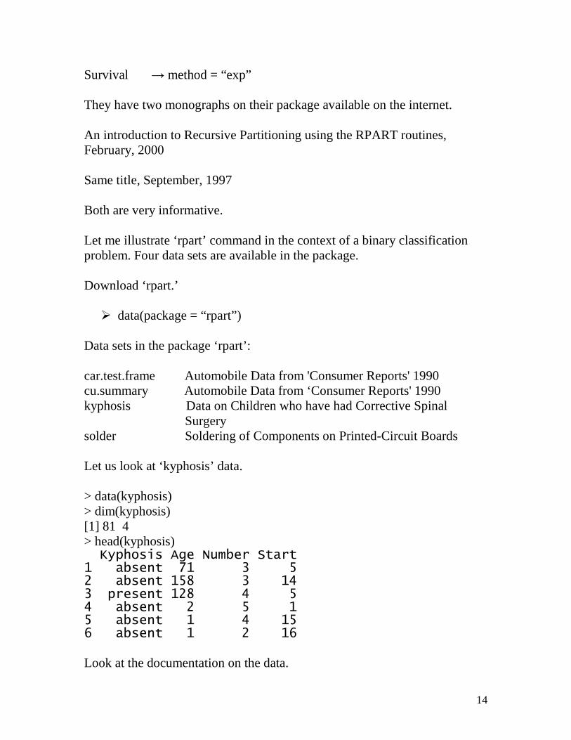
= 100*(8 + 0 + 2 + 3)/81 = 16%. We have other choices when graphing a tree. Let us try some of these. > plot(MB, branch = 0, margin = 0.1, col = "red") > text(MB, use.n = T, all = T, col = "red") > title(MB, main = "Classification Tree for Kyphosis data") The graph is below.

18

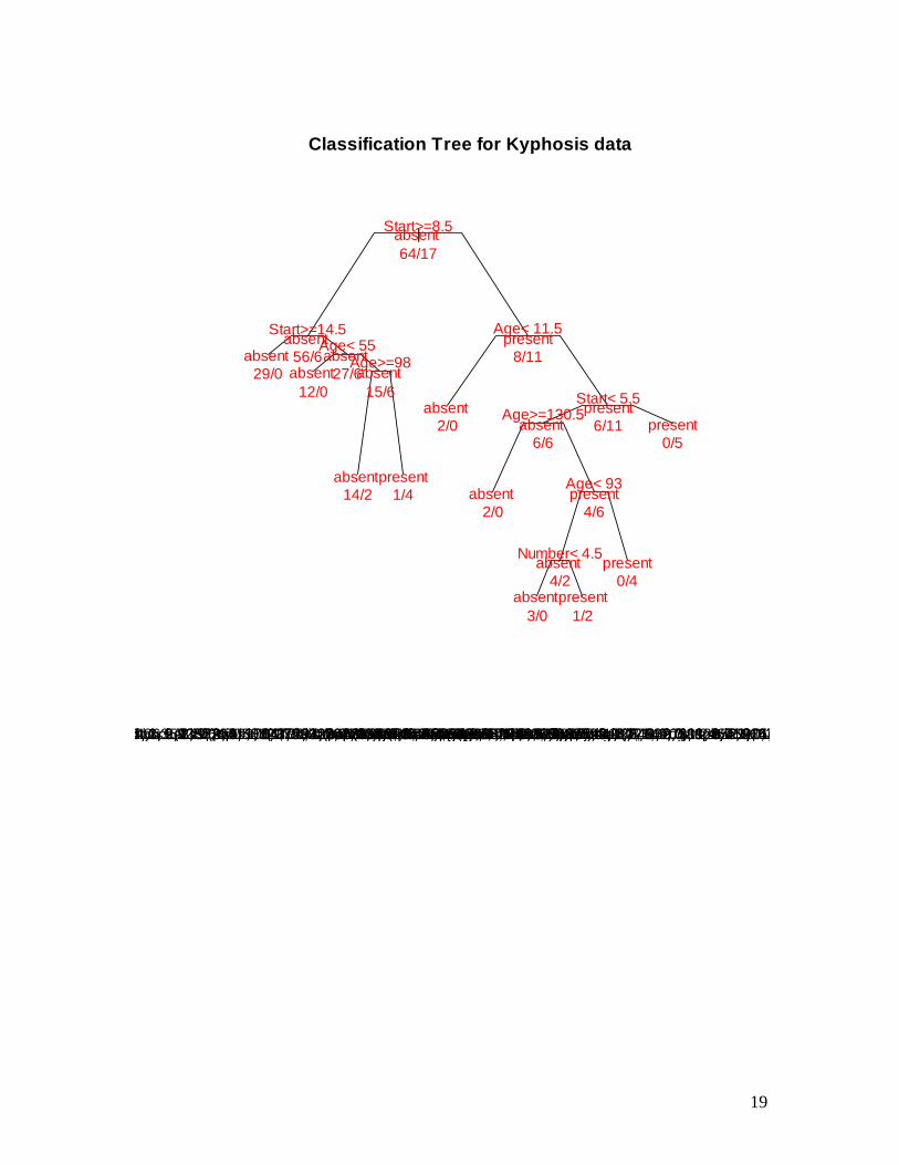
> plot(MB, branch = 0.4, margin = 0.1, col = "red") > text(MB, use.n = T, all = T, col = "red") > title(MB, main = "Classification Tree for Kyphosis data") The graph is on Page 12.

Start>=8.5

Start>=14.5Age< 55

Age>=111

absent 64/17

absent 56/6absent

29/0absent

27/6absent 12/0

absent 15/6

absent 12/2

present3/4

present8/11

Classification Tree for Kyphosis data

list(var = c(4, 4, 1, 2, 1, 2, 1, 1, 1), n = c(81, 62, 29, 33, 12, 21, 14, 7, 19), wt = c(81, 62, 29, 33, 12, 21, 14, 7, 19), dev = c(17, 6, 0, 6, 0, 6, 2, 3, 8), yval = c(1, 1, 1, 1, 1, 1, 1, 2, 2), complexity = c(0.176470588235294, 0.0196078431372549, 0.01, 0.0196078431372549, 0.01, 0.019607, 5, 3, 9, 8, 9, 9, 5, 9, 8, 3, 3, 3, 7, 7, 3, 7, 3, 5, 9, 5, 8, 9, 5, 9, 9, 3, 7, 3, 7, 9, 7, 8, 3, 9, 3, 3, 3, 5, 9, 5, rpart(formula = Kyphosis ~ ., data = kyphosis)Kyphosis ~ Age + Number + Start, 4, 1, 0.823529411764706, 0.764705882352941, 1, 1.17647058823529, 1.17647058823529, 0.2c(81, 81, 81, 0, 62, 62, 62, 0, 0, 33, 33, 33, 0, 0, 21, 21, 21, 1, -1, -1, -1, 1, -1, -1, -1, -1, -1, 1, 1, -1, 1, 1, 1, 1, 6.76232995870801, 2.86679493346161, 2.25021151687820, 0.80246913580247, 1.02052785923755, 0.684863523573199, 0.297533206831119, 0.64516129032258, 0.596774193548387, 1.246753246classlist(prior = c(0.790123456790123, 0.209876543209877), loss = c(0, 1, 1, 0), split = 1)list(minsplit = 20, minbucket = 7, cp = 0.01, maxcompete = 4, maxsurrogate = 5, usesurrogate = 2, surrogatestyle = 0, maxdepth = 30, xval = 10)list(summary = function (yval, dev, wt, ylevel, digits) , 1, 1, 2, 2, 1, 2, 1, 1, 1, 1, 1, 1, 1, 1, 1, 1, 1, 1, 2, 1, 2, 2, 1, 1, 1, 1, 2, 1, 1, 2, 1, 1, 1, 2, 1, 1, 1, 1, 2, 1, c(FALSE, FALSE, FALSE)

19

|Start>=8.5

Start>=14.5Age< 55

Age>=98

Age< 11.5

Start< 5.5Age>=130.5

Age< 93

Number< 4.5

absent 64/17

absent 56/6absent

29/0absent

27/6absent 12/0

absent 15/6

absent 14/2

present1/4

present8/11

absent 2/0

present6/11absent

6/6

absent 2/0

present4/6

absent 4/2

absent 3/0

present1/2

present0/4

present0/5



20

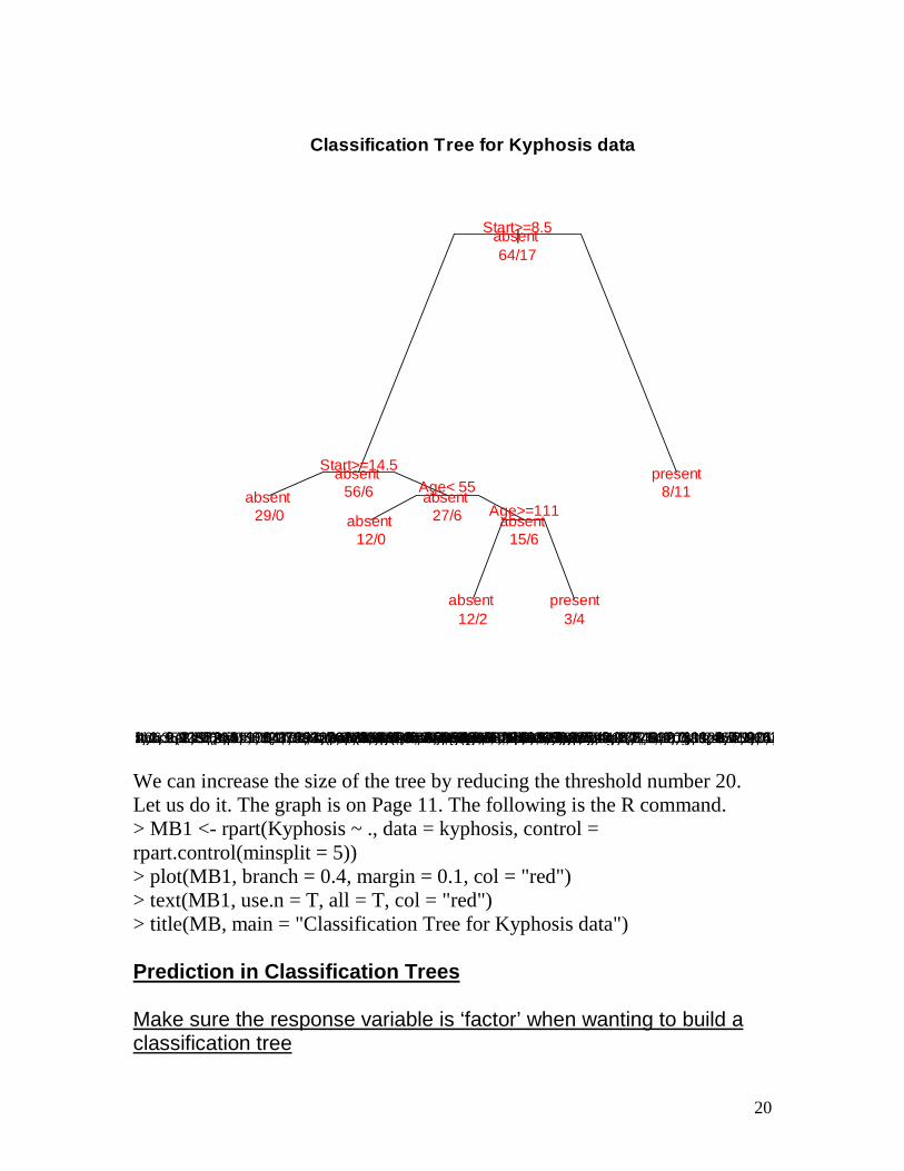
We can increase the size of the tree by reducing the threshold number 20. Let us do it. The graph is on Page 11. The following is the R command. > MB1 <- rpart(Kyphosis ~ ., data = kyphosis, control = rpart.control(minsplit = 5)) > plot(MB1, branch = 0.4, margin = 0.1, col = "red") > text(MB1, use.n = T, all = T, col = "red") > title(MB, main = "Classification Tree for Kyphosis data") Prediction in Classification Trees Make sure the response variable is ‘factor’ when wanting to build a classification tree

|Start>=8.5

Start>=14.5Age< 55

Age>=111

absent 64/17

absent 56/6absent

29/0absent

27/6absent 12/0

absent 15/6

absent 12/2

present3/4

present8/11



21

We build classification trees when the response variable is binary. If you use rpart package, make sure your response variable is a ‘factor.’ If the response variable is descriptive such as absence and presence, the response variable is indeed a ‘factor.’ If the response variable is coded as 0 and 1, make sure the codes are factors. If they are not, one can always convert them into factors using the command ‘as.factor.’ Suppose the file is called MB. Then type < MB <- as.factor(MB). Prediction in classification trees Let us work with the kyphosis data. Activate the ‘rpart’ package. > data(kyphosis) Build a classification tree. > MB <- rpart(Kyphosis ~ ., data = kyphosis) The ‘predict’ command predicts the status of each kid in the data as per the classification tree. > MB1 <- predict(MB, newdata = kyphosis) > head(MB1) absent present 1 0.4210526 0.5789474 2 0.8571429 0.1428571 3 0.4210526 0.5789474 4 0.4210526 0.5789474 5 1.0000000 0.0000000 6 1.0000000 0.0000000 What is going on? Look at the data. > head(kyphosis) Kyphosis Age Number Start 1 absent 71 3 5 2 absent 158 3 14 3 present 128 4 5 4 absent 2 5 1 5 absent 1 4 15 6 absent 1 2 16 Look at the first kid. Feed his data into the tree. He falls into the last terminal node. The prediction as per the tree is ‘Kyphosis present.’ Look at the data in the last terminal node. Nineteen of our kids will fall into this node. Eight of them have Kyphosis absent and eleven of

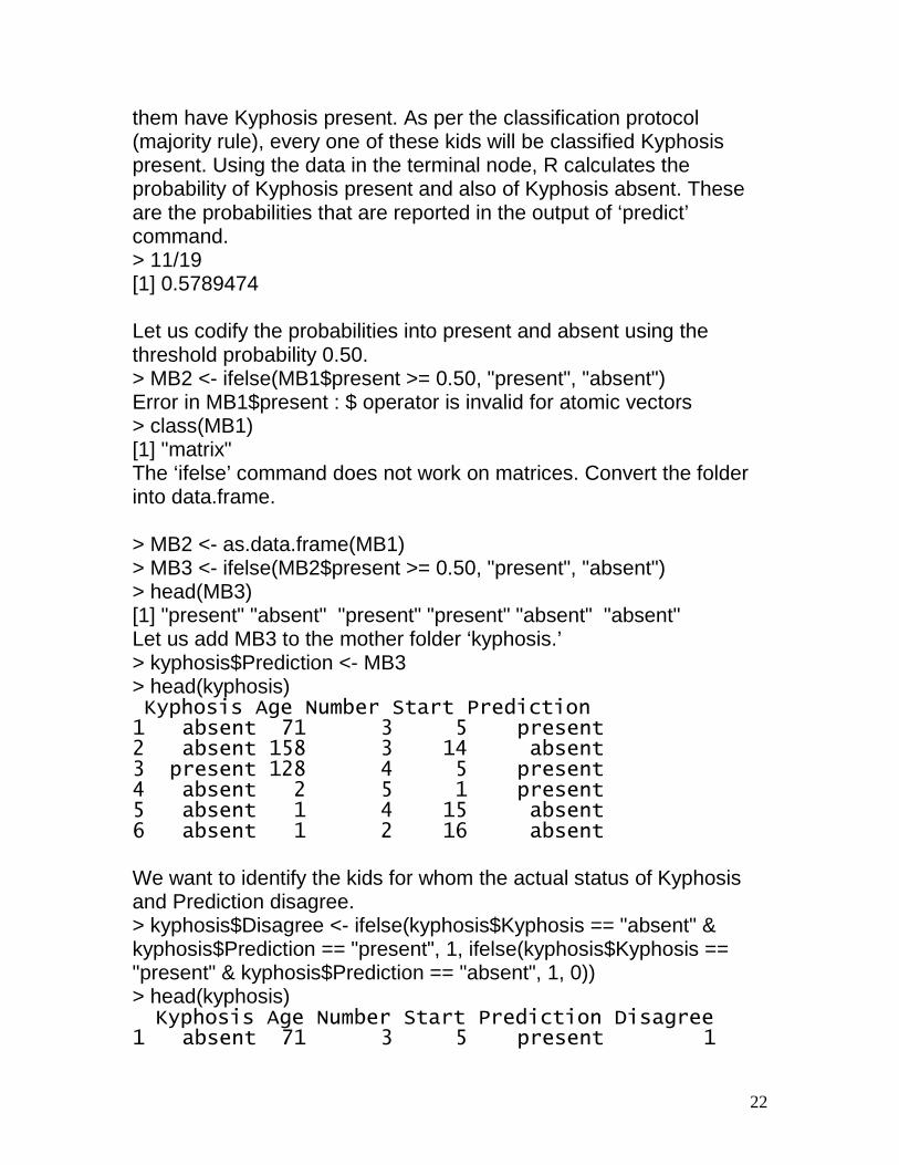
22

them have Kyphosis present. As per the classification protocol (majority rule), every one of these kids will be classified Kyphosis present. Using the data in the terminal node, R calculates the probability of Kyphosis present and also of Kyphosis absent. These are the probabilities that are reported in the output of ‘predict’ command. > 11/19 [1] 0.5789474 Let us codify the probabilities into present and absent using the threshold probability 0.50. > MB2 <- ifelse(MB1$present >= 0.50, "present", "absent") Error in MB1$present : $ operator is invalid for atomic vectors > class(MB1) [1] "matrix" The ‘ifelse’ command does not work on matrices. Convert the folder into data.frame. > MB2 <- as.data.frame(MB1) > MB3 <- ifelse(MB2$present >= 0.50, "present", "absent") > head(MB3) [1] "present" "absent" "present" "present" "absent" "absent" Let us add MB3 to the mother folder ‘kyphosis.’ > kyphosis$Prediction <- MB3 > head(kyphosis) Kyphosis Age Number Start Prediction 1 absent 71 3 5 present 2 absent 158 3 14 absent 3 present 128 4 5 present 4 absent 2 5 1 present 5 absent 1 4 15 absent 6 absent 1 2 16 absent We want to identify the kids for whom the actual status of Kyphosis and Prediction disagree. > kyphosis$Disagree <- ifelse(kyphosis$Kyphosis == "absent" & kyphosis$Prediction == "present", 1, ifelse(kyphosis$Kyphosis == "present" & kyphosis$Prediction == "absent", 1, 0)) > head(kyphosis) Kyphosis Age Number Start Prediction Disagree 1 absent 71 3 5 present 1

23

2 absent 158 3 14 absent 0 3 present 128 4 5 present 0 4 absent 2 5 1 present 1 5 absent 1 4 15 absent 0 6 absent 1 2 16 absent 0 How many kids are misclassified? > sum(kyphosis$Disagree) [1] 13 What is the misclassification rate? > (13/81)*100 [1] 16.04938 We have two new kids with the following information. Kid 1 Age = 12; Number = 4; Start = 7 Kid 2 Age = 121; Number = 5, Start = 9 How does the tree classify these kids? > MB4 <- data.frame(Age = c(12, 121), Number = c(4, 5), Start = c(7, 9)) > MB4 Age Number Start 1 12 4 7 2 121 5 9 > MB5 <- predict(MB, newdata = MB4) > MB5 absent present [1,] 0.4210526 0.5789474 [2,] 0.8571429 0.1428571 The first kid will be classified as Kyphosis present and the second Kyphosis absent. Regression trees We now focus on developing a regression tree when the response variable is quantitative. Let me work out the build-up of a tree using an example. The data set ‘bodyfat’ is available in the package ‘mboost.’ Download the package and the data. The data has 71 observations on 10 variables. Body fat was measured on 71 healthy German women using Dual Energy X-ray Absorptiometry (DXA). This reference method is very accurate in measuring body fat. However, the setting-up of this instrument

24

requires a lot of effort and is of high cost. Researchers are looking ways to estimate body fat using some anthropometric measurements such as waist circumference, hip circumference, elbow breadth, and knee breadth. The data gives these anthropometric measurements on the women in addition to their age. Here is the data. > data(bodyfat) > dim(bodyfat) [1] 71 10 > head(bodyfat) age DEXfat waistcirc hipcirc elbowbreadth kneebreadth anthro3a anthro3b 47 57 41.68 100.0 112.0 7.1 9.4 4.42 4.95 48 65 43.29 99.5 116.5 6.5 8.9 4.63 5.01 49 59 35.41 96.0 108.5 6.2 8.9 4.12 4.74 50 58 22.79 72.0 96.5 6.1 9.2 4.03 4.48 51 60 36.42 89.5 100.5 7.1 10.0 4.24 4.68 52 61 24.13 83.5 97.0 6.5 8.8 3.55 4.06 anthro3c anthro4 47 4.50 6.13 48 4.48 6.37 49 4.60 5.82 50 3.91 5.66 51 4.15 5.91 52 3.64 5.14

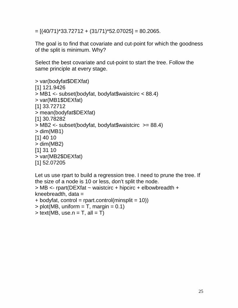
Ignore the last four measurements. Each one is a sum of logarithms of three of the four anthropometric measurements. We now want to create a regression tree. All data points go into the root node to begin with. We need to select one of the covariates and a cut-point to split the root node. In the case of classification trees, the choice is guided by ‘entropy.’ In the case of regression trees, the choice is guided by ‘variance.’ Let us start with the covariate ‘waistcirc’ and the cut-point 88.4, say. All women with waistcirc < 88.4 are shepherded into the left node and the rest into the right node. We need to judge how good the split is. As hinted earlier, we use variance as the criterion. Calculate the variance of ‘DEXfat’ of all women in the root node. It is 121.9426. Calculate the variance of ‘DEXfat’ of all women in the left node. It is 33.72712. Calculate the variance of ‘DEXfat’ of all women in the right node. It is 52.07025. Goodness of the split = Weighted sum of daughters’ variances

25

= [(40/71)*33.72712 + (31/71)*52.07025] = 80.2065. The goal is to find that covariate and cut-point for which the goodness of the split is minimum. Why? Select the best covariate and cut-point to start the tree. Follow the same principle at every stage. > var(bodyfat$DEXfat) [1] 121.9426 > MB1 <- subset(bodyfat, bodyfat$waistcirc < 88.4) > var(MB1$DEXfat) [1] 33.72712 > mean(bodyfat$DEXfat) [1] 30.78282 > MB2 <- subset(bodyfat, bodyfat$waistcirc >= 88.4) > dim(MB1) [1] 40 10 > dim(MB2) [1] 31 10 > var(MB2$DEXfat) [1] 52.07205 Let us use rpart to build a regression tree. I need to prune the tree. If the size of a node is 10 or less, don’t split the node. > MB <- rpart(DEXfat ~ waistcirc + hipcirc + elbowbreadth + kneebreadth, data = + bodyfat, control = rpart.control(minsplit = 10)) > plot(MB, uniform = T, margin = 0.1) > text(MB, use.n = T, all = T)

26

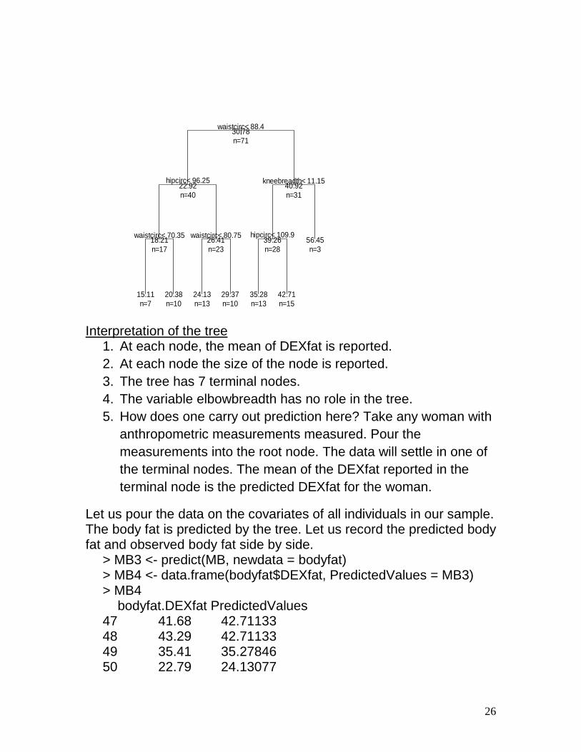
Interpretation of the tree

1. At each node, the mean of DEXfat is reported. 2. At each node the size of the node is reported. 3. The tree has 7 terminal nodes. 4. The variable elbowbreadth has no role in the tree. 5. How does one carry out prediction here? Take any woman with

anthropometric measurements measured. Pour the measurements into the root node. The data will settle in one of the terminal nodes. The mean of the DEXfat reported in the terminal node is the predicted DEXfat for the woman.

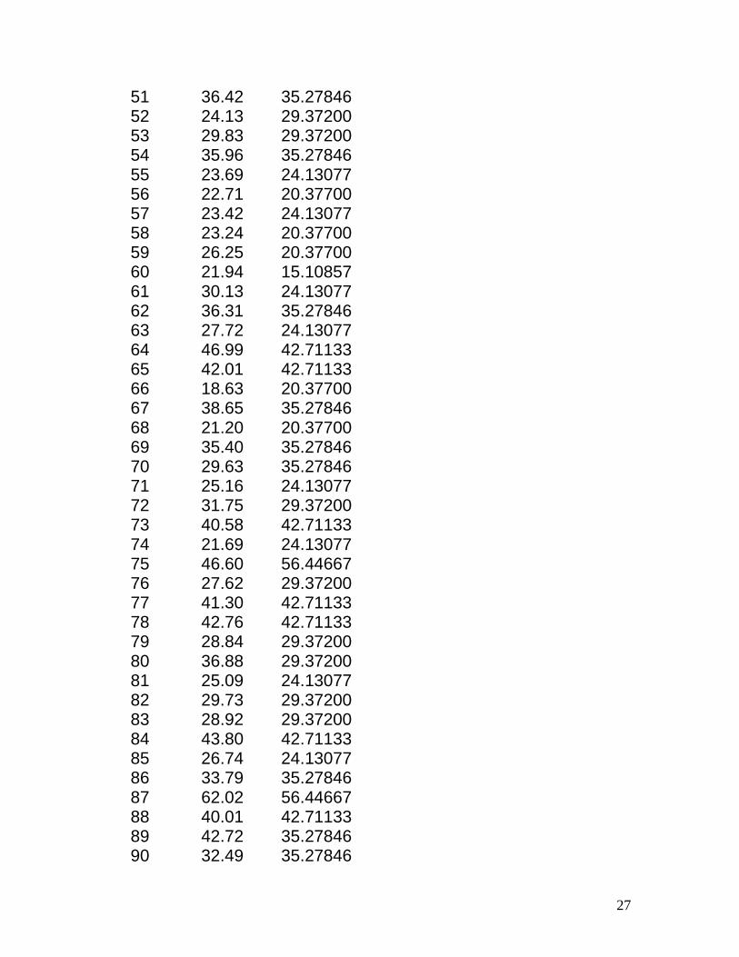
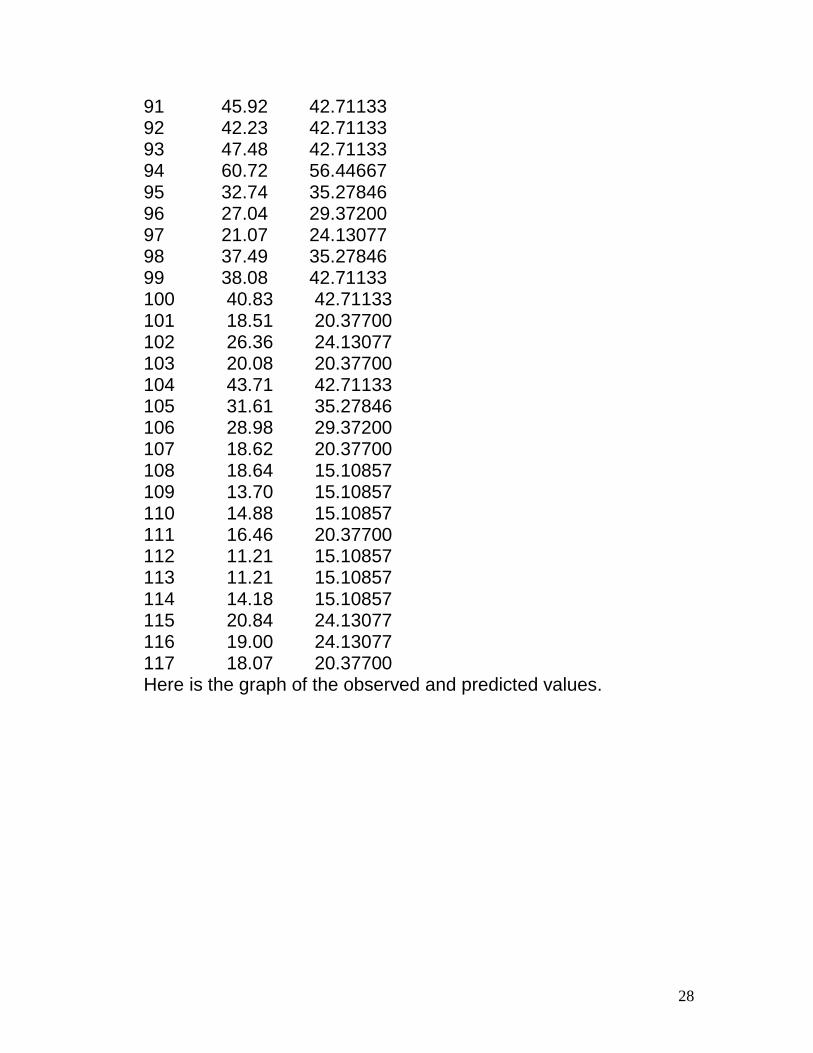
Let us pour the data on the covariates of all individuals in our sample. The body fat is predicted by the tree. Let us record the predicted body fat and observed body fat side by side.

> MB3 <- predict(MB, newdata = bodyfat) > MB4 <- data.frame(bodyfat$DEXfat, PredictedValues = MB3) > MB4 bodyfat.DEXfat PredictedValues 47 41.68 42.71133 48 43.29 42.71133 49 35.41 35.27846 50 22.79 24.13077

|waistcirc< 88.4

hipcirc< 96.25

waistcirc< 70.35 waistcirc< 80.75

kneebreadth< 11.15

hipcirc< 109.9

30.78n=71

22.92n=40

18.21n=17

15.11n=7

20.38n=10

26.41n=23

24.13n=13

29.37n=10

40.92n=31

39.26n=28

35.28n=13

42.71n=15

56.45n=3

27

51 36.42 35.27846 52 24.13 29.37200 53 29.83 29.37200 54 35.96 35.27846 55 23.69 24.13077 56 22.71 20.37700 57 23.42 24.13077 58 23.24 20.37700 59 26.25 20.37700 60 21.94 15.10857 61 30.13 24.13077 62 36.31 35.27846 63 27.72 24.13077 64 46.99 42.71133 65 42.01 42.71133 66 18.63 20.37700 67 38.65 35.27846 68 21.20 20.37700 69 35.40 35.27846 70 29.63 35.27846 71 25.16 24.13077 72 31.75 29.37200 73 40.58 42.71133 74 21.69 24.13077 75 46.60 56.44667 76 27.62 29.37200 77 41.30 42.71133 78 42.76 42.71133 79 28.84 29.37200 80 36.88 29.37200 81 25.09 24.13077 82 29.73 29.37200 83 28.92 29.37200 84 43.80 42.71133 85 26.74 24.13077 86 33.79 35.27846 87 62.02 56.44667 88 40.01 42.71133 89 42.72 35.27846 90 32.49 35.27846

28

91 45.92 42.71133 92 42.23 42.71133 93 47.48 42.71133 94 60.72 56.44667 95 32.74 35.27846 96 27.04 29.37200 97 21.07 24.13077 98 37.49 35.27846 99 38.08 42.71133 100 40.83 42.71133 101 18.51 20.37700 102 26.36 24.13077 103 20.08 20.37700 104 43.71 42.71133 105 31.61 35.27846 106 28.98 29.37200 107 18.62 20.37700 108 18.64 15.10857 109 13.70 15.10857 110 14.88 15.10857 111 16.46 20.37700 112 11.21 15.10857 113 11.21 15.10857 114 14.18 15.10857 115 20.84 24.13077 116 19.00 24.13077 117 18.07 20.37700 Here is the graph of the observed and predicted values.

29

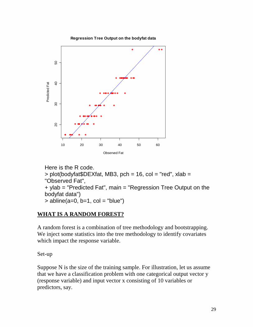
Here is the R code. > plot(bodyfat$DEXfat, MB3, pch = 16, col = "red", xlab = "Observed Fat", + ylab = "Predicted Fat", main = "Regression Tree Output on the bodyfat data") > abline(a=0, b=1, col = "blue")

WHAT IS A RANDOM FOREST? A random forest is a combination of tree methodology and bootstrapping. We inject some statistics into the tree methodology to identify covariates which impact the response variable. Set-up Suppose N is the size of the training sample. For illustration, let us assume that we have a classification problem with one categorical output vector y (response variable) and input vector x consisting of 10 variables or predictors, say.

10 20 30 40 50 60

2030

4050

Regression Tree Output on the bodyfat data

Observed Fat

Pre

dict

ed F

at

30

We build a tree. We may not use all original data. We may not use all predictors. Step 1 Select a random sample of size N with replacement from the training data. What does this mean? All these data go into the root node. We need to split the node into two daughter nodes. Step 2 Choose and fix an integer 1 < m < 10. Select a random sample of m predictors without replacement from the set of 10 predictors on hand. From this sample of m predictors, choose the best predictor to split the root node into two daughter nodes in the usual way either using entropy or Gini’s index in impurity calculations. (We should have a thorough understanding of classification tree procedure here.) Step 3 We need to split the daughter nodes. Take the ‘left daughter node.’ Select a random sample of m predictors without replacement from the set of all predictors. From this sample of m predictors, choose the best predictor to split the node. For the ‘right daughter node,’ select a random sample of m predictors without replacement from the set of all predictors. From this sample of m predictors, choose the best predictor to split the node. Step 4 We will now have four grand daughters. Split each of these nodes the same way as outlined in Step 2 or 3. Step 5 Continue this process until we cannot proceed further. No pruning is done. We will have a very large tree. Step 6 Repeat Steps 1 to 5 500 times. Thus we will have 500 trees. This is the so called random forest.

31

How do we classify a new data vector x? Feed the vector into each of the trees. Find out what the majority of these trees say. (Condorcet principle) The vector x is classified accordingly. This is essentially ‘bagging’ procedure with randomization on predictors introduced at every node for splitting! Let us look at the package ‘randomForest.’ Download this package and make it active. Look at its documentation. The documentation is attached.

� ?randomForest A discussion of inputs 1. The first input x is the matrix of data on predictors, The second input is the corresponding data on the response variable (class or quantitative). In lieu of these inputs, one can give a formula. 2. ntree = number of trees. The default is set at 500 3. mtry = fixed number of predictors to be selected randomly at every node. The default is set at the integer part of the square root of the number of predictors. 4. importance: with respect to every category in the response one gets information how important the predictors in classification. Importance = F is the default. (To be explained later) 5. proximity: the command calculates proximity scores between any two rows of the input data.

The result is a NxN matrix. Let us apply the command on the ‘iris’ data. Download the data. > data(iris) Understand the data. > head(iris) Sepal.Length Sepal.Width Petal.Length Petal.Width Species 1 5.1 3.5 1.4 0.2 setosa

32

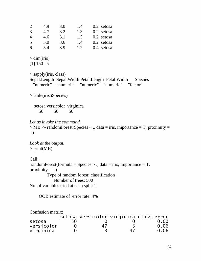
2 4.9 3.0 1.4 0.2 setosa 3 4.7 3.2 1.3 0.2 setosa 4 4.6 3.1 1.5 0.2 setosa 5 5.0 3.6 1.4 0.2 setosa 6 5.4 3.9 1.7 0.4 setosa > dim(iris) [1] 150 5 > sapply(iris, class) Sepal.Length Sepal.Width Petal.Length Petal.Width Species "numeric" "numeric" "numeric" "numeric" "factor" > table(iris$Species) setosa versicolor virginica 50 50 50 Let us invoke the command. > MB <- randomForest(Species ~ ., data = iris, importance = T, proximity = T) Look at the output. > print(MB) Call: randomForest(formula = Species ~ ., data = iris, importance = T, proximity = T) Type of random forest: classification Number of trees: 500 No. of variables tried at each split: 2 OOB estimate of error rate: 4% Confusion matrix: setosa versicolor virginica class.error setosa 50 0 0 0.00 versicolor 0 47 3 0.06 virginica 0 3 47 0.06

33

Understand the output. 1. R says that this is a classification problem. 2. R produces a forest of 500 trees. 3. There are four predictors. At every node, it chose 2 predictors at random. 4. The given data were poured into the root node. The acronym ‘OOB’ stands for ‘out-of-bag.’ The OOB (error) estimate is 4%. The confusion matrix spells out where errors of misclassification occurred. What else is available in the output folder “MB.’ > names(MB) [1] "call" "type" "predicted" "err.rate" [5] "confusion" "votes" "oob.times" "classes" [9] "importance" "importanceSD" "localImportance" "proximity" [13] "ntree" "mtry" "forest" "y" [17] "test" "inbag" "terms" Let us look at ‘importance.’ > round(importance(MB), 2)

setosa versicolor virginica MeanDecreaseAccuracy MeanDecreaseGini

Sepal.Length 1.54 1.70 1.75 1.35 9.61 Sepal.Width 1.04 0.30 1.19 0.72 2.28 Petal.Length 3.62 4.40 4.18 2.48 41.68 Petal.Width 3.88 4.43 4.26 2.52 45.68 Interpretation of the output 1. For setosa, the most important variable that played a role in the classification is Petal.Width followed by Petal.Length. The same story is valid for every other flower. 2. Since Petal.Length and Petal.Width are consistently important for every species, it means for classification purpose, we could use only these two variables. I have a new flower whose identity is unknown. I know its measurements: 6.1, 3.9, 1.5, 0.5. We want to classify this flower. Pour these measurements

34

into the root node of every tree in the forest. See what the majority says. This is a prediction problem. > MB1 <- data.frame(Sepal.Length = 6.1, Sepal.Width = 3.9, Petal.Length = 1.5, Petal.Width = 0.5) > MB1 Sepal.Length Sepal.Width Petal.Length Petal.Width 1 6.1 3.9 1.5 0.5 > MB2 <- predict(MB, newdata = MB1, type = "class") > MB2 [1] setosa Levels: setosa versicolor virginica This flower is classified as setosa. One can obtain a graph of the importance of the predictors in the classification problem. Here is the relevant R code. > varImpPlot(MB, pch = 16, col = "red", n.var = 4, sort = T, main = "Importance of + Variables for the Iris data")

35

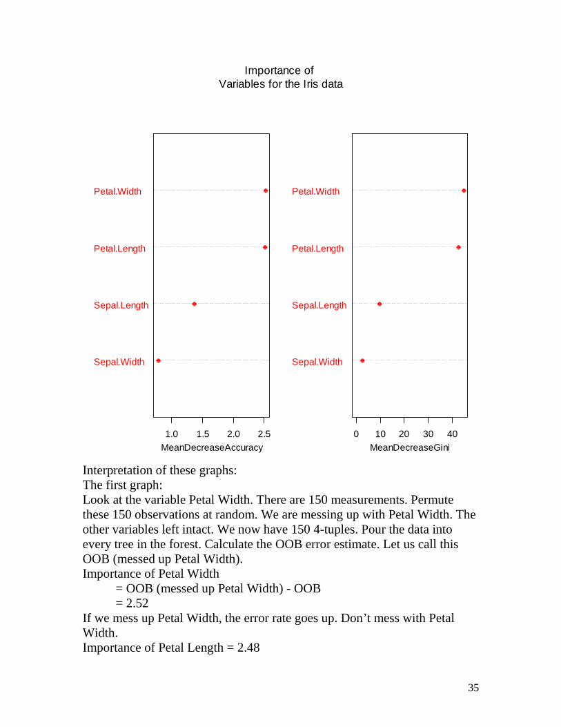
Interpretation of these graphs: The first graph: Look at the variable Petal Width. There are 150 measurements. Permute these 150 observations at random. We are messing up with Petal Width. The other variables left intact. We now have 150 4-tuples. Pour the data into every tree in the forest. Calculate the OOB error estimate. Let us call this OOB (messed up Petal Width). Importance of Petal Width

= OOB (messed up Petal Width) - OOB = 2.52

If we mess up Petal Width, the error rate goes up. Don’t mess with Petal Width. Importance of Petal Length = 2.48

Sepal.Width

Sepal.Length

Petal.Length

Petal.Width

1.0 1.5 2.0 2.5MeanDecreaseAccuracy

Sepal.Width

Sepal.Length

Petal.Length

Petal.Width

0 10 20 30 40MeanDecreaseGini

Importance of Variables for the Iris data

36

Importance of Sepal Length = 1.35 Importance of Sepal Width = 0.72 The second graph: When a tree is created, the best predictor is selected to split any node. One can calculate how much improvement is achieved by the best split over the mother node using Gini’s index. Identify all the nodes at which this predictor appeared and note down how much the percentage improvement. Take the average of all these improvements over all trees in the forest. This average is the importance of this predictor as per Gini. Gini’s improvement index (Petal Width) = 45.68% Ginis’ improvement index (Petal Length) = 41.68% Gini’s improvement index (Sepal Length) = 9.61% Gini’s improvement index (Sepal Width) = 2.28% Important lessons learned We can see that Petal Width and Petal Length are the most important predictors of the genus of the flower. We could suggest that one could use only these two measurements in the classification. We now come to big data set. We need a big stick. Data and analysis courtesy of : Ms. Weng Zhouyang (a graduate student in our department) and Dr. Mersha, CCHMC Thousand-genome project Seven different populations are being studied genetically. How one can characterize each population genetically? Populations with sample sizes in brackets

1. CEPH – Caucasians from the United States with Northern and Western European Ancestry (90)

2. Toscans from Italy (66) 3. Han Chinese from Beijing (109) 4. Chinese from Denver (107) 5. Japanese from Tokyo (105) 6. Yoruba from Ibadan, Nigeria (112) 7. Luhya Webuye from Kenya (108)

Each member of the sample is genotyped at 1379 SNPs.

37

Objective: If I know the data of an individual on these 1379 SNPs, will I be able to predict which population he is coming from? This is a classification or pattern recognition problem.

1. The response variable is categorical with 7 levels. 2. The number of covariates is 1379. 3. Each covariate is ternary (genotypes).

Incidental objective. Do I need data on all these SNPs for the classification problem? The data are ripe for an application of random forest methodology. Output Table 1: Confusion Matrix from Random Forest Model OOB estimate of error rate: 22.96%

CEPH Denver Chinese

Han Chinese Japanese Luhya Tuscan Yoruba Class.error

CEPH 77 0 0 0 0 13 0 0.1444Denver Chinese 0 68 17 22 0 0 0 0.3645Han Chinese 0 30 56 23 0 0 0 0.4862Japanese 0 4 13 88 0 0 0 0.1619Luhya 0 0 0 0 107 0 1 0.0093Tuscan 11 0 0 0 0 55 0 0.1667Yoruba 0 0 0 0 26 0 86 0.2321

Features of analysis

1. A forest is built with 1000 trees. The value m = 200 was chosen to split each node in each tree of the forest. At these choices the out-of-bag error estimate stabilizes at 22.96%.

2. Look at the table. Errors of misclassification are clustered. Three clusters emerge.

Denver Chinese + Han Chinese + Japanese CEPH + Tuscans Yoruba + Luhya

38

No one from each cluster is mis-classified.

3. This analysis leads us to focus on these clusters separately.

Table 2: Variable Importance Plot (top 20 SNP variables)

Are these SNPs good enough to carry the entire mantle of classification? We did a random forest on the ‘iris’ data. Let us do a classification tree for demonstration. > data(iris) > iris$SL <- iris$Sepal.Length > iris$SW <- iris$Sepal.Width > iris$PL <- iris$Petal.Length > iris$PW <- iris$Petal.Width > head(iris) Sepal.Length Sepal.Width Petal.Length Petal.Width Species SL SW PL PW 1 5.1 3.5 1.4 0.2 setosa 5.1 3.5 1.4 0.2 2 4.9 3.0 1.4 0.2 setosa 4.9 3.0 1.4 0.2 3 4.7 3.2 1.3 0.2 setosa 4.7 3.2 1.3 0.2

SNP47SNP511SNP481SNP337SNP34SNP734SNP804SNP1345SNP40SNP304SNP1352SNP656SNP674SNP974SNP1076SNP517SNP1071SNP1075SNP1153SNP1210

0.6 0.7 0.8 0.9 1.0MeanDecreaseAccuracy

SNP505SNP542SNP1076SNP183SNP1071SNP687SNP1352SNP481SNP1153SNP337SNP511SNP1075SNP760SNP610SNP974SNP656SNP674SNP40SNP304SNP1210


Importance of Variables

39

4 4.6 3.1 1.5 0.2 setosa 4.6 3.1 1.5 0.2 5 5.0 3.6 1.4 0.2 setosa 5.0 3.6 1.4 0.2 6 5.4 3.9 1.7 0.4 setosa 5.4 3.9 1.7 0.4 > MB <- rpart(Species ~ SL + SW + PL + PW, data = iris) > plot(MB, uniform = T, margin = 0.1) > text(MB , use.n = T, all = T) > title(main = "Classificatin Tree for the iris data")

Interpretation? CROSS-VALIDATION IN RANDOM FORESTS + OCCUPATIONAL ASTHMA DATA A preamble We have data from NIOSH, Morgantown, West Virginia. The subjects of the study come from a number of work environments such as sawmills, steel foundries, etc. The subjects are divided into two groups: those who are diagnosed to have occupational asthma (cases) (Group 2) and those who do not have asthma (controls) (Group 5). Blood samples are drawn from the participants of the study and data on more than 2,000 SNPs are collected. A genome wide association analysis is carried out and seven SNPs stood out to be significant after the Bonferroni adjustment. Measurements on 8

|PL< 2.45

PW< 1.75

setosa 50/50/50

setosa 50/0/0

versicolor0/50/50

versicolor0/49/5

virginica 0/1/45

Classificatin Tree for the iris data

40

demographic variables are collected on each participant. I have the data in my flash drive. Download the data onto R. Input the data into R. > read.xls("C:\\Rprojects\\Berran2v5SnpCov.xls") -> MB Look at the top six rows of the data. > head(MB) Sampleid GroupC rs1264457 rs1573294 rs1811197 rs3128935 rs4711213 rs7773955 1 CAN235 2 1 1 2 1 3 1 2 CAN237 2 1 1 3 1 3 1 3 CAN242 2 1 3 3 1 3 1 4 CAN260 2 1 2 3 2 3 1 5 CAN263 2 1 2 3 1 3 1 6 CIN309 2 1 1 2 1 3 1 rs928976 Sex Age Height ExpMonths Atopy1 Smoking PackYears 1 2 M 30.00000 173 172.0 pos ex 6.0 2 1 M 23.00000 184 7.0 neg current 4.0 3 1 M 19.00000 175 13.0 pos never 0.0 4 2 M 38.00000 178 34.7 pos ex 5.0 5 1 M 58.00000 170 346.4 pos ex 31.3 6 3 M 26.16389 173 76.8 pos never 0.0

Check the dimension of the data. > dim(MB) [1] 159 16 Response variable: GroupC Variables SNPs: rs1264457 rs1573294 rs1811197 rs3128935 rs4711213 rs7773955 rs928976 Demographics: Sex Age Height ExpMonths Atopy1 Smoking PackYears

41

Remove the individuals on whom demographics are missing. Remove the id too. > MB1 <- MB[-c(81, 87, 95, 133, 146, 149), -1] > dim(MB1) [1] 153 15 What kind of variable is GroupC? > class(MB1[ , 1]) [1] "numeric" Convert that into a categorical variable. > MB1[ , 1] <- as.factor(MB1[ , 1]) > class(MB1[ , 1]) [1] "factor" The goal is cross-validation. We want to set aside 1/3rd of the data randomly selected. Perform random forest methodology on the remaining 2/3rd of the data. > n <- dim(MB1)[1] > n [1] 153 > k <- (2/3)*n > k [1] 102 Select a random sample of 102 numbers from 1 to 153. > s <- sample(1:n, k) > s [1] 54 20 89 49 15 135 82 76 4 113 136 22 125 59 142 42 63 144 [19] 83 130 35 146 61 116 78 16 74 44 123 106 81 140 80 52 12 55 [37] 68 112 117 88 134 126 53 138 11 151 67 28 107 60 40 109 95 121 [55] 72 104 29 31 128 79 43 98 65 10 86 108 87 105 77 101 129 18 [73] 30 1 19 90 58 69 57 71 149 124 26 115 66 93 152 21 102 137 [91] 120 70 41 32 119 131 143 122 47 150 36 51

Create the learning set of 102 individuals. > MBLset <- MB1[s, ] Create the test set of 51 individuals.

� MBTset <- MB1[ -s, ]

42

The learning set had 51 individuals belonging to Group 2 and 50 belonging to Group 5. This is good. > table(MBLset[ , 1]) 2 5 52 50 Run the random forest method on the learning set. > model.rf <- randomForest(GroupC ~ ., data = MBLset, importance = T) Look at the output. > print(model.rf) Call: randomForest(formula = GroupC ~ ., data = MBLset, importance = T, proximity = T) Type of random forest: classification Number of trees: 500 No. of variables tried at each split: 3 OOB estimate of error rate: 10.78% Confusion matrix: 2 5 class.error 2 45 7 0.1346154 5 4 46 0.0800000 Comments on the output: Each node is split using 3 randomly selected covariates. A forest of 500 trees is created. The learning sample was poured into the trees. The majority rule was used. The out-of-bag (OOB) error (misclassifications) was 10.78%. Which covariates played an important role in the groups. The importance measure is given below. > round(model.rf$importance, 3) 2 5 MeanDecreaseAccuracy MeanDecreaseGini rs1264457 0.088 0.101 0.093 9.493 rs1573294 0.007 0.024 0.016 3.156 rs1811197 0.010 0.002 0.006 1.739 rs3128935 0.035 0.017 0.026 3.848 rs4711213 0.025 0.018 0.021 2.949 rs7773955 0.030 0.013 0.022 3.304 rs928976 0.016 0.018 0.017 3.799 Sex 0.000 0.001 0.000 0.183 Age 0.032 0.064 0.046 8.654 Height -0.002 0.003 0.000 2.656

43

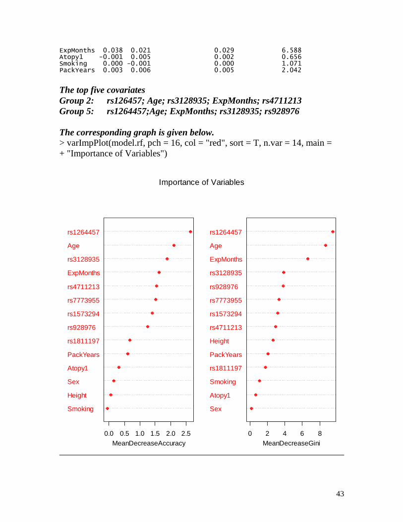
ExpMonths 0.038 0.021 0.029 6.588 Atopy1 -0.001 0.005 0.002 0.656 Smoking 0.000 -0.001 0.000 1.071 PackYears 0.003 0.006 0.005 2.042

The top five covariates Group 2: rs126457; Age; rs3128935; ExpMonths; rs4711213 Group 5: rs1264457;Age; ExpMonths; rs3128935; rs928976 The corresponding graph is given below. > varImpPlot(model.rf, pch = 16, col = "red", sort = T, n.var = 14, main = + "Importance of Variables")

Smoking

Height

Sex

Atopy1

PackYears

rs1811197

rs928976

rs1573294

rs7773955

rs4711213

ExpMonths

rs3128935

Age

rs1264457

0.0 0.5 1.0 1.5 2.0 2.5MeanDecreaseAccuracy

Sex

Atopy1

Smoking

rs1811197

PackYears

Height

rs4711213

rs1573294

rs7773955

rs928976

rs3128935

ExpMonths

Age

rs1264457


Importance of Variables

44

The test set is used for prediction. > predict.rf <- predict(model.rf, newdata = MBTset, type = "class") The accuracy of prediction is determined. > acc.rf <- 100*sum(predict.rf == MBTset$GroupC)/dim(MBTset)[1] Prediction accuracy is 92.15%. > acc.rf [1] 92.15686 Further exploration The default value for m (= number of variables randomly selected to carry out splits at each node) is sqrt(number of covariates) rounded to the lower number. One can ask R to choose m optimally with the view to minimize OOB (out-of-bag) error rate. The relevant command is ‘tuneRF.’ A documentation of this command is included. If time permits, we will work on this command. Cross-validation in Random Forests + De Loop + Model Comparison Let us work with the NIOSH Asthma data. The response variable is GroupC (5 = Occupational Asthma, 2 = No Asthma). We want to do a random forest analysis to identify important covariates and determine the OOB (Out of Bag Error Estimate). We want to obtain a 95% confidence interval for the true OOB. This can be obtained by the cross-validation method. The basic steps are:

1. Select a 70% random sample of the data. This is the training sample. The subjects that are not in the sample constitute the test sample. Total number of subjects in the entire sample is 140. Seventy percent of 140 work out to be 98. The size of the test sample is 42.

2. Perform random forest analysis on the chosen training sample. 3. Predict GroupC for the test sample. 4. Calculate the OOB of the test sample. 5. Repeat Steps 1 through 4 ninety-nine times more. 6. We will now have 100 OOBs. Build a 95% confidence interval for the

true OOB.

45

This requires two loops. The first loop will have to generate one-hundred 70% samples from the index set 1:140. The second loop will calculate OOB for each of the one-hundred test samples. Activate the package ‘randomForest’ and make the binary variable ‘GroupC’ categorical. Download the data from the blackboard by copying the data in a ‘clipboard.’ Open R Editor. Asthma <- read.table(“clipboard”) We now type all our commands in the R Editor. > dim(Asthma) [1] 140 13 > head(Asthma) GroupC rs1573294 rs1811197 rs3128935 rs7773955 rs928976 Sex Age Height 1 5 AG GG AG AA CT M 38.3 178 2 2 AA AG AA AA CC M 26.2 173 3 2 AA GG AA AA CC M 28.6 180 4 2 AA GG AA AA TT M 25.9 180 5 2 GG GG AA AG CT M 32.8 183 6 2 AG GG AA AA CC M 27.6 188 ExpMonths Atopy1 Smoking Packyrs 1 34.7 pos ex 5.0 2 76.8 pos never 0.0 3 69.6 neg never 0.0 4 82.8 neg current 9.8 5 74.4 pos never 0.0 6 76.8 neg current 5.6

How many have occupational asthma. > table(Asthma$GroupC) 2 5 67 73 Make ‘GroupC’ as factor. > Asthma$GroupC <- as.factor(Asthma$GroupC) Let us generate one-hundred random samples of size 98 with replace = F (default). Create a matrix of order 98 x 100 consisting of zeros as a prelude to the loop. > Training <- matrix(0, 98, 100) For the loop, create an index set. > Index <- 1:100 The i-th column of the matrix ‘Training’ is filled with a 70% random sample. > for (i in Index) + {

46

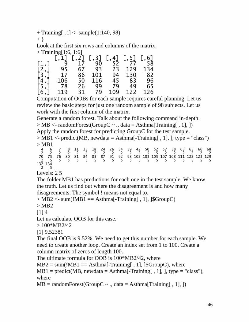
+ Training[ , i] <- sample(1:140, 98) + } Look at the first six rows and columns of the matrix. > Training[1:6, 1:6] [,1] [,2] [,3] [,4] [,5] [,6] [1,] 9 17 90 52 77 58 [2,] 95 67 93 23 129 134 [3,] 17 86 101 94 130 82 [4,] 106 50 116 45 83 96 [5,] 78 26 99 79 49 65 [6,] 119 31 79 109 122 126 Computation of OOBs for each sample requires careful planning. Let us review the basic steps for just one random sample of 98 subjects. Let us work with the first column of the matrix. Generate a random forest. Talk about the following command in-depth. > MB <- randomForest(GroupC ~ ., data = Asthma[Training[ , 1], ]) Apply the random forest for predicting GroupC for the test sample. > MB1 <- predict(MB, newdata = Asthma[-Training[ , 1], ], type = "class") > MB1 4 6 7 8 11 15 18 24 26 34 39 42 50 52 57 58 63 65 66 68 2 2 2 2 2 2 2 2 2 2 2 2 5 5 2 2 2 2 2 2 70 75 76 80 81 84 85 87 91 92 98 102 103 105 107 108 111 122 123 129 2 5 5 5 5 5 5 5 5 5 5 5 5 5 5 5 5 5 5 5 132 134 2 5

Levels: 2 5 The folder MB1 has predictions for each one in the test sample. We know the truth. Let us find out where the disagreement is and how many disagreements. The symbol ! means not equal to. > MB2 <- sum(!MB1 == Asthma[-Training[ , 1], ]$GroupC) > MB2 [1] 4 Let us calculate OOB for this case. > 100*MB2/42 [1] 9.52381 The final OOB is 9.52%. We need to get this number for each sample. We need to create another loop. Create an index set from 1 to 100. Create a column matrix of zeros of length 100. The ultimate formula for OOB is 100*MB2/42, where MB2 = sum(!MB1 == Asthma[-Training[ , 1], ]$GroupC), where MB1 = predict(MB, newdata = Asthma[-Training[ , 1], ], type = "class"), where MB = randomForest(GroupC ~ ., data = Asthma[Training[ , 1], ])

47

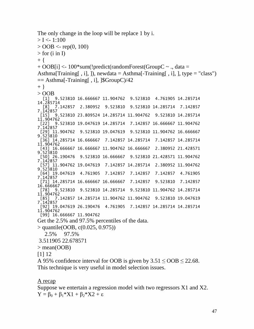
The only change in the loop will be replace 1 by i. > I <- 1:100 > OOB <- rep(0, 100) > for (i in I) + { + OOB[i] <- 100*sum(!predict(randomForest(GroupC ~ ., data = Asthma[Training[ , i], ]), newdata = Asthma[-Training[ , i], ], type = "class") == Asthma[-Training[ , i], ]$GroupC)/42 + } > OOB [1] 9.523810 16.666667 11.904762 9.523810 4.761905 14.285714 14.285714 [8] 7.142857 2.380952 9.523810 9.523810 14.285714 7.142857 7.142857 [15] 9.523810 23.809524 14.285714 11.904762 9.523810 14.285714 11.904762 [22] 9.523810 19.047619 14.285714 7.142857 16.666667 11.904762 7.142857 [29] 11.904762 9.523810 19.047619 9.523810 11.904762 16.666667 9.523810 [36] 14.285714 16.666667 7.142857 14.285714 7.142857 14.285714 11.904762 [43] 16.666667 16.666667 11.904762 16.666667 2.380952 21.428571 9.523810 [50] 26.190476 9.523810 16.666667 9.523810 21.428571 11.904762 7.142857 [57] 11.904762 19.047619 7.142857 14.285714 2.380952 11.904762 9.523810 [64] 19.047619 4.761905 7.142857 7.142857 7.142857 4.761905 7.142857 [71] 14.285714 16.666667 16.666667 7.142857 9.523810 7.142857 16.666667 [78] 9.523810 9.523810 14.285714 9.523810 11.904762 14.285714 11.904762 [85] 7.142857 14.285714 11.904762 11.904762 9.523810 19.047619 7.142857 [92] 19.047619 26.190476 4.761905 7.142857 14.285714 14.285714 11.904762 [99] 16.666667 11.904762

Get the 2.5% and 97.5% percentiles of the data. > quantile(OOB, c(0.025, 0.975)) 2.5% 97.5% 3.511905 22.678571 > mean(OOB) [1] 12 A 95% confidence interval for OOB is given by 3.51 ≤ OOB ≤ 22.68. This technique is very useful in model selection issues. A recap Suppose we entertain a regression model with two regressors X1 and X2. Y = β0 + β1*X1 + β2*X2 + ε

48

Fit this model to the data. Let us call the output folder MB. Suppose we want to entertain two additional covariates X3 and X4. We want to try the model Y = β0 + β1*X1 + β2*X2 + β3*X3 + β4*X4 + ε Note that the first model is nested into the second model. The question we raise is whether the two additional covariates will increase our understanding of the response variable Y. This is tantamount testing H0: β3 = β4 = 0. Go ahead and fit this model. Let the output folder be MB1. In R, we can use the command < anova(MB, MB1) to test the null hypothesis H0. The output will give the p-value associated with H0. When will this work?

1. One model is nested into the other. 2. Both models use the same data. Explain this further.

What is an analogue of model selection in the environment of random forests? Let us look at the NIOSH occupational asthma problem.

1. I want to develop a prediction model using only the SNP data. 2. Is it worthwhile adding all the demographic variables to the model?

Method 1. Conduct a cross-validation study using only the SNPs. Build a 95%

confidence interval for OOB. Call this interval I1. 2. Conduct a cross-validation study using SNPs and all demographic

variables. Build a 95% confidence interval for OOB. Call this interval I2.

3. If the intervals are disjoint, we can conclude that adding the demographic variables reduces OOB significantly.

Bagging and Boosting – An Introduction + What is bagging? + What is boosting? Regression and Classification are two of the most widely used statistical methodologies in scientific and social research. If the response variable or output is quantitative, regression methodologies come to the fore no matter what the inputs are. If the response variable or output is a class

49

label, classification techniques rule the roost. I have used the following methodologies in regression in my consulting work.

1. Neural networks 2. Traditional multiple regression 3. Regression trees 4. Support vector machines 5. Bayesian networks 6. Lasso 7. Least Angle Regression 8. Spline Regression

In the case of classification, the choice is good.

1. Neural networks 2. Classification trees 3. Fisher’s Linear Discriminant Function 4. Fisher’s Quadratic Discriminant Function 5. Nonparametric classification 6. Support vector machines 7. Logistic regression 8. Bayesian networks

In the case of regression, the purpose of a model is to carry out prediction. For a given input x (possibly, a vector) what will be the output y? Using training data {(xn, yn); n = 1, 2, … , N} of input and output on N cases, we strive to build a good model connecting the output y with input x so as to reduce the prediction error as much as possible. In the case of classification, the purpose is to classify a given input into one of a set of classes. Using training data {(xn, yn); n = 1, 2, … , N} of input and output on N cases, we strive to put in place a good classification protocol so as to reduce misclassifications as much as possible. Bagging, Boosting, and Random Forests are three of the latest techniques developed in this connection. I will now present basic ideas involved in the first two methodologies. The proponents of these methods try to convince us that these methods work better than the existing methods in the sense that they reduce prediction error or misclassification rates as the case may be. The following data sets have been used as battle grounds for testing the new methodologies. I will follow their route.

50

The heart data of San Diego Medical Center.

When a heart patient is admitted, information is gathered on 19

variables x1, x2, … , x19 during the first 24 hours. The variables include blood pressure, age, and 17 other ordered binary variables summarizing the medical symptoms considered as important indicators of the patient’s condition. The goal of collecting data is to develop a method of identifying high risk patients (those who will not survive at least 30 days) on the basis of the initial 24-hour data. The data consist of information on 779 patients. Of these, 77 patients died within 30 days of admittance and the remaining were survivors. This is a problem in classification. For a heart patient admitted to the hospital, let y = 1 if the patient dies with in 30 days of admittance, = 0 if the patient survives at least 30 days. The y-variable is a class variable. For each patient in the data set, we have an input x~ = (x1, x2, … , x19) and an output y. Using the data {( nn yx ,~ ); n = 1, 2, … , 779} on 779 patients, we want to develop a classification protocol. The protocol is essentially of the form

y = f( x~), where for each input x~, y = 1 or zero. Suppose some one provides us with a classification protocol. We want to judge how good the protocol is.

We can apply the given classification protocol to the data on hand. For Patient No. 1, we know the input 1

~x (all the nineteen measurements) and output y1 (whether or not he/she died within 30 days). We can find out what the classification protocol says to the input 1

~x . Find out what the y value is for the input 1

~x . Calculate 1y = f( 1~x ). This means that we are predicting

what will happen to the patient using the classification protocol. We do know what exactly happened y1 to him. The entities y1 and 1y may not agree. If they agree, the protocol classified Patient No. 1 correctly. If not, we say that a misclassification occurred. We can execute these steps for every patient in the data set. We can calculate the total number of misclassifications and the misclassification rate. This misclassification rate is used to judge the quality of the classification protocol.

51

What is the ultimate goal for building a classification protocol? Suppose we have a new heart patient wheeled into the hospital. In the next 24 hours we gather information on 19 variables x1, x2, … , x19. The doctors-in-charge are curious: is he/she going to survive at least 30 days? The classification protocol they have is very reliable. Check what the protocol says. Feed the input into the protocol. See how the patient is classified.

The classification protocol in place could be very revealing. We will

try to understand among the 19 inputs which ones are the most dominant. We may focus on these dominant inputs and advise patients accordingly.

I know many methods of building classification protocols. Depending

on the availability of resources, I can try all the methods and then recommend one with the least misclassification rate. Leo Breiman, in a seminal paper – Bagging Predictors, Machine Learning, 24, 123-140, 1996, proposed a new method of building a classification protocol. He proclaimed that the misclassification rate stemming from his new method is the lowest. Is it really? We will see. Breast Cancer Data of University of Wisconsin Hospitals The researchers at the hospitals collected data 699 patients. How the data were collected? A patient comes into a clinic. A lump is detected in a breast. A sample of breast tissue is sent to the lab for analysis. The result: the lump is either benign or malignant. On each patient measurements on 9 variables consisting of cellular characteristics are taken. Input x1 = Clump thickness on a scale 1 to 10 x2 = Uniformity of cell size (1 – 10) x3 = Uniformity of cell shape (1 – 10) x4 = Marginal adhesion (1 – 10) x5 = Single epithelial cell size (1 – 10) x6 = Bare nuclei (1 – 10) x7 = Bland chromatin (1 – 10) x8 = Normal nucleoli (1 – 10) x9 = Mitosis (1 – 10) Output

52

y = 2 if the clump is benign, = 4 if the clump is malignant. The measurements on the input variables are easy to procure. Taking a sample of breast tissue is painful and lab analysis expensive. If we know the input x~ = (x1, x2, … , x9) on a patient, can we predict the output? This is again a classification problem. Does the Bagging Procedure provide a good classification protocol with misclassification rate very, very low? Diabetes Data of Pima Indians by the National Institute of Diabetes and Digestive and Kidney Diseases The data base consists of 768 cases, 8 variables and two classes. The variables are medical measurements on the patient plus age and pregnancy information. The classes are: tested positive for diabetes (268) or negative (500). Determining whether or not a patient is diabetic is not an easy job. Are there biomarkers which can help us the determination? Spliced DNA sequence data of the Genbank For each subject in the sample, a certain window of 60 nucleotides is looked at. Input x1 = The nucleotide in the first position of the window (Possible values: A, G, C, T) x2 = The nucleotide in the second position of the window (A, G, C, T) … … … x60 = The nucleotide in the 60th position of the window (A, G, C, T). Output Look at the middle of the window. It has a Boundary of Type 1, Boundary of Type 2, or neither. The output is a class variable with three classes.

53

This is again a classification problem. Boston Housing It has 506 cases corresponding to census tracts in the greater Boston area. Input It has 12 predictor variables, mainly socio-economic. Output The y-variable is the median housing price in the tract. This is a regression problem. Ozone data The data consist of 366 readings of maximum daily ozone at a hot spot in the Los Angeles basin and 9 predictor variables – all meteorological, i.e., temperature, humidity, etc. Soybean data The data consist of 683 cases, 35 variables (input) and 19 classes (output). The classes are various types of soybean diseases. The variables are observations on the plants together with some climatic variables.

There is a website devoted to Boosting. www.boosting.org The website has tutorials and research papers. You get to know who is who in Bagging and Boosting. My plan

1. I will outline the basic idea of bagging. Explain how this method improves misclassification rate in comparison with the Classification Tree methodology.

2. I will outline the basic idea of boosting. Illustrate its use on some data sets.

54

3. R procedures are now extensively available to execute all these procedures. We will learn some of these commands.

What is bagging? Set-up We have data on a response variable y and a predictor x for N individual cases. The predictor x is typically multi-dimensional and the response variable y is either quantitative or a class variable. The data are denoted by

Ł = {(y n, xn); n = 1, 2, … , N}. In computer science literature, Ł is called a learning set. The primary goal in data analysis is to build a model

y = φ(x, Ł) connecting the predictor x to the response variable y using the learning set Ł. Once we have the model in place, we can predict the response y for any given input x. The predicted value of y is φ(x, Ł). I am assuming that you have a method to produce the predictor φ(x, Ł). You might have used a neural network, traditional multiple regression methodology in the case the response variable is quantitative, logistic regression in the case the response variable is binary, a support vector machine, a regression tree, or a classification tree, etc. You choose your own methodology you are comfortable with to carry out the task of developing the prediction equation y = φ(x, Ł). Suppose you are given a sequence Łk, k = 1, 2, … , M of training sets. Each training set has N cases generated in the same way as the original one Ł. These training sets are replicates of Ł. Using your own chosen methodology, build the prediction equation

y = φ(x, Łk) for each training set Łk, the same way you built φ(x, Ł). Thus we will have M prediction equations. It is natural that we should combine all prediction equations into a single one.

55

Suppose the response variable y is quantitative. Define for any input x,

φA(x) = (1/M)∑=

M

k 1ϕ (x, Łk).

We are averaging all the predictors! The subscript A stands for ‘aggregation.’ Suppose the response variable y is a class variable. Let the classes be denoted by 1, 2, … , J. For a given input x, let N1 = #{1 ≤ k ≤ M; φ(x, Łk) = 1}, N2 = #{1 ≤ k ≤ M; φ(x, Łk) = 2}, … … … NJ = #{1 ≤ k ≤ M; φ(x, Łk) = J}. The entity N1 is the number of prediction equations each of which classifies the object x into Class 1, etc. Define for an input x, φA(x) = i, if Ni is the maximum of {N1, N2, … , NJ}. The object x is classified into Class i if the majority of the prediction equations classify x into Class i. In other words, the aggregate classification is done by voting. Usually, we have a single learning set Ł without the luxury of replicates of Ł. In order to generate replicates of the given training set, we resort to bootstrapping. Training set Treat the training set as population. Population: (y1, x1) (y2, x2) … (yN, xN) Prob.: 1/N 1/N … 1/N Our population consists of N units. The i-th unit is attached with the entity (yi, xi). Draw a random sample of size N from the population with replacement. This is called a Bootstrap Sample. Denote this Bootstrap Sample by Ł(1). Using the replicate Ł(1), build the predictor φ(x, Ł(1)) just the way you built φ(x, Ł) using the same methodology.

56

Bootstrap again and again generating M Bootstrap Samples Ł(1), Ł(2), …, Ł(M). Build the corresponding predictors φ s. The construction of prediction equation requires a clarification. Suppose y is a class variable. For example, suppose you use classification tree methodology to build the prediction equation y = φ(x, Ł). You should use the classification tree methodology to build the prediction equation for each Bootstrap Sample Ł(k). Carry out aggregation in the usual way as outlined above. This procedure is called ‘bootstrap aggregating.’ The acronym ‘bagging’ is used for this procedure. This is not a new methodology. This is an enhancement of whatever methodology you use in building a prediction equation. Evidence, both experimental and theoretical, suggests that bagging improves the accuracy of your chosen methodology of building prediction equations. When does bagging improve accuracy? It depends how stable the selected methodology is. A methodology is said to be unstable if small changes in the training set Ł result in big changes in the prediction equation y = φ(x, Ł). Talk about this a little bit more.

Breiman (1994, Annals of Statistics, Heuristics of instability in model selection) showed that neural networks, regression trees, classification trees, and subset selection in the linear regression are unstable. The k-nearest neighbor method is stable.

If your chosen methodology is unstable, bagging improves accuracy.

This is intuitively clear. If the methodology is unstable, a Bootstrap Sample of Ł will induce big changes in the prediction equation y = φ(x, Ł). Therefore, aggregation of repeated Bootstrap Samples can only improve the accuracy of the prediction equation. If your chosen methodology is stable, bagging might slightly degrade accuracy.

Talk about the original purpose of the bootstrap technique. Efron and Tibshirani (1993) – An Introduction to Bootstrap, Chapman

and Hall.

57

Breiman (Combining Artificial Neural Networks, Ed. Amanda Sharkey, Springer, 1999) reports a number of data sets and compares the performances of Bagging and Boosting with the underlying core methodology of classification being Classification Trees (CART). Data Set Size A B Error Error Error Rate Rate Rate CART Boost Bag Heart 1395 2 16 4.9 1.1 2.8 Breast Cancer 699 2 9 5.9 3.2 3.7 Ionosphere 351 2 34 11.2 6.4 7.9 Diabetes 768 2 8 25.3 26.6 23.9 Glass 214 6 9 30.4 22.0 23.2 Soybean 683 19 35 8.6 5.8 6.8 Letters 15,000 26 16 12.4 3.4 6.4 Satellite 4435 6 36 14.8 8.8 10.3 Shuttle 43500 7 9 0.062 0.007 0.014 DNA 2000 3 60 6.2 4.2 5.0 Digit 7291 10 256 27.1 6.2 10.5 Legend: A = # Classes B = # Variables CART: Classification Tree Methodology

The Classification Tree Methodology was performed on each data once and the corresponding error rate is recorded. For Bagging and Boosting, the CART is the preferred methodology of classification. What is Boosting? Let me explain the ‘boosting’ methodology in the context of a binary classification problem. Before we invoke the ‘Boosting’ paradigm, we must choose a classification methodology.

58

Let us get back to a binary classification problem. We have a training sample of size N. We need to develop a classification protocol based on the training sample. Data (Training Sample) ( 1~x , y1) ( 2

~x , y2) … ( Nx~ , yN)

Each ix~ is an n-component vector. Each yi is either +1 or -1. The entity -1

signifies that the i-th individual belongs to Group 1 and +1 indicates that the individual belongs to Group 2. Step 1 Write down your training sample with uniform weights. Sample: (1

~x , y1) ( 2~x , y2) … ( Nx~ , yN)

Weights: w11 w12 … w1N 1/N 1/N … 1/N

Use your preferred method of classification to find an optimal classifier f1. Freund and Schapire (1966), the originators of ‘Boosting,’ used Neural Networks. Statisticians usually use CART. At this stage, the weights play no role in the development of the classifier. Calculate the error rate err1 associated with the classifier f1. (We are judging how good the classifier is.) If f 1( 1

~x ) = y1 (correct classification), error is zero. If f 1( 1

~x ) ≠ y1 (wrong classification), error is one. Etc. Observation Error Weight ( 1~x , y1) e11 (1 or 0) w11

( 2~x , y2) e12 (1 or 0) w12

… … … ( Nx~ , yN) e1N (1 or 0) w1N

Error rate = err1 = w11e11 + w12e12 + … + w1Ne1N

59

err1 is precisely the proportion of times observations are misclassified by the classifier f1.

Calculate c1 = ln 1

11err

err− c1 is called learning coefficient.

If err1 = 0 or ≥ 1/2 , stop. If err1 = 0, we have hit on the perfect classifier. There is no need to proceed further. Use f1. If err1 ≥ ½, this is worse than the flipping-coin classification protocol. You cannot proceed further. Abandon the chosen classification methodology. Try a different one. Step 2 Calculate a new set of weights. w21 = w11exp(c1e11) w22 = w12exp(c1e12) … … w2N = w1Nexp(c1e1N) If ix~ is correctly classified, e1i = 0 and hence w2i = w1i. If ix~ is incorrectly

classified, e1i = 1 and hence w2i = w1i (1

11

err

err−). Note that w2i is larger than

w1i. The new weights are normalized. They are adjusted so that their sum is unity. I use the same notation for the new weights. Write the data with new weights. Sample: (1

~x , y1) ( 2~x , y2) … ( Nx~ , yN)

Weights: w21 w22 … w2N (Sum = 1) Misclassified observations get more weight! Use the weighted version of your chosen classification methodology to get classifier f2. What does this mean? We have a population consisting of N entities:

60

( 1~x , y1), ( 2

~x , y2), … , ( Nx~ , yN). There is a probability distribution w21, w22, … , w2N over these entities. Draw a random sample of size N with replacement from this population according to this distribution. Some duplication is possible. If an entity has a large weight, this entity will have many duplicates in the drawn sample. Let the new sample be denoted by,

( *1

~x , *1y ) ( *

2~x , *

2y ) … ( *~Nx , *

Ny ) Each entity here is one of the original entities. Use your own preferred methodology to get a classifier f2. Calculate the error rate err2 associated with f2. Use the original training sample.

If f 2( 1~x ) = y1 (correct classification), error is zero.

If f 2( 1~x ) ≠ y1 (wrong classification), error is one.

Etc. Observation Error Weight ( 1~x , y1) e21 (1 or 0) w21

( 2~x , y2) e22 (1 or 0) w22

… … … ( Nx~ , yN) e2N (1 or 0) w2N

Error rate = err2 = w21e21 + w22e22 + … + w2Ne2N err2 is precisely the weighted proportion of times observations are misclassified.

Calculate c2 = ln 2

21

err

err−. c2 is the learning coefficient coming from the

classifier f2. If err2 = 0, stop, we have hit the perfect classifier. If err2 ≥ ½, stop. Your chosen methodology is useless. Step 3 Calculate a new set of weights in exactly the same way the weights are calculated in Step 2 following Step 1.

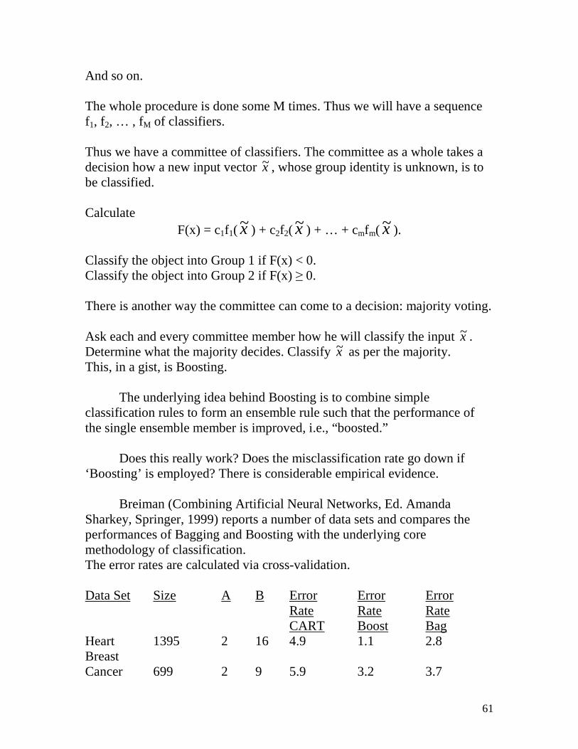
61

And so on. The whole procedure is done some M times. Thus we will have a sequence f1, f2, … , fM of classifiers. Thus we have a committee of classifiers. The committee as a whole takes a decision how a new input vector x~, whose group identity is unknown, is to be classified. Calculate

F(x) = c1f1( x~ ) + c2f2( x~ ) + … + cmfm( x~ ). Classify the object into Group 1 if F(x) < 0. Classify the object into Group 2 if F(x) ≥ 0. There is another way the committee can come to a decision: majority voting. Ask each and every committee member how he will classify the input x~. Determine what the majority decides. Classify x~ as per the majority. This, in a gist, is Boosting.

The underlying idea behind Boosting is to combine simple classification rules to form an ensemble rule such that the performance of the single ensemble member is improved, i.e., “boosted.” Does this really work? Does the misclassification rate go down if ‘Boosting’ is employed? There is considerable empirical evidence. Breiman (Combining Artificial Neural Networks, Ed. Amanda Sharkey, Springer, 1999) reports a number of data sets and compares the performances of Bagging and Boosting with the underlying core methodology of classification. The error rates are calculated via cross-validation. Data Set Size A B Error Error Error Rate Rate Rate CART Boost Bag Heart 1395 2 16 4.9 1.1 2.8 Breast Cancer 699 2 9 5.9 3.2 3.7

62

Ionosphere 351 2 34 11.2 6.4 7.9 Diabetes 768 2 8 25.3 26.6 23.9 Glass 214 6 9 30.4 22.0 23.2 Soybean 683 19 35 8.6 5.8 6.8 Letters 15,000 26 16 12.4 3.4 6.4 Satellite 4435 6 36 14.8 8.8 10.3 Shuttle 43500 7 9 0.062 0.007 0.014 DNA 2000 3 60 6.2 4.2 5.0 Digit 7291 10 256 27.1 6.2 10.5 Legend: A = # Classes B = # Variables CART: Classification Tree Methodology The Classification Tree Methodology was performed on each data once and the corresponding error rate is recorded. For Bagging and Boosting, the CART is the preferred methodology of classification. Bagging and Boosting with R Let us work with the ‘iris’ data. Recall that the data set has three species of flowers. The response variable is categorical with 3 levels. > data(iris) > dim(iris) [1] 150 5 > head(iris) Sepal.Length Sepal.Width Petal.Length Petal.Width Species 1 5.1 3.5 1.4 0.2 setosa 2 4.9 3.0 1.4 0.2 setosa 3 4.7 3.2 1.3 0.2 setosa 4 4.6 3.1 1.5 0.2 setosa 5 5.0 3.6 1.4 0.2 setosa 6 5.4 3.9 1.7 0.4 setosa

> table(iris$Species) setosa versicolor virginica 50 50 50 What shall we do?

1. Use a random subset of the data to build a prediction model. Check how good the model is for the unused data. Try classification methodology.

2. Use all data. Try classification methodology.

63

3. Try Boosting. 4. Try Bagging. Project. 5. Try other methods of classification. Project.

Let us not use all data. Select randomly 25 flowers from setosa, 25 from versicolor, and 25 from virginica. Create the indices first. > Sample <- c(sample(1:50, 25), sample(51:100, 25), sample(101:150, 25)) > Sample [1] 20 29 26 28 38 35 34 31 19 13 7 22 43 12 18 32 8 16 11 [20] 49 42 36 9 21 48 61 86 80 51 64 90 85 98 97 67 52 77 65 [39] 56 55 88 57 84 75 69 100 60 58 63 89 127 120 128 145 132 129 122 [58] 107 140 149 123 102 108 137 110 133 131 101 117 124 147 119 150 116 135

Let us get the training sample. > Training <- iris[Sample, ] > dim(Training) [1] 75 5 Let us do a classification tree just once. Activate the ‘rpart’ package. > Once <- rpart(Species ~ ., data = Training, control = rpart.control(minsplit = 10)) > plot(Once, uniform = T, margin = 0.1) > text(Once, use.n = T, all = T) > title(main = "Classification Tree of Iris data Randomly Chosen", sub = "Size = 75") > 1/75 [1] 0.01333333 The tree is given on Page 13. Let us do boosting. Download and activate the ‘adaboost’ package. Let us have only 10 trees. Let us prune the trees at the size 10. > Boost <- boosting(Species ~ ., data = Training, mfinal = 10, control = + rpart.control(minsplit = 10)) > Boost $formula Species ~ . Each tree is described. $trees $trees[[1]] n= 75 node), split, n, loss, yval, (yprob) * denotes terminal node 1) root 75 49 setosa (0.34666667 0.33333333 0.32000000) 2) Petal.Length< 2.5 26 0 setosa (1.00000000 0.00000000 0.00000000) * 3) Petal.Length>=2.5 49 24 versicolor (0.00000000 0.51020408 0.48979592) 6) Petal.Length< 4.85 26 1 versicolor (0.00000000 0.96153846 0.03846154) * 7) Petal.Length>=4.85 23 0 virginica (0.00000000 0.00000000 1.00000000) *

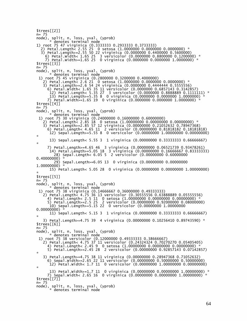
64

$trees[[2]] n= 75 node), split, n, loss, yval, (yprob) * denotes terminal node 1) root 75 47 virginica (0.3333333 0.2933333 0.3733333) 2) Petal.Length< 2.55 25 0 setosa (1.0000000 0.0000000 0.0000000) * 3) Petal.Length>=2.55 50 22 virginica (0.0000000 0.4400000 0.5600000) 6) Petal.Width< 1.65 25 3 versicolor (0.0000000 0.8800000 0.1200000) * 7) Petal.Width>=1.65 25 0 virginica (0.0000000 0.0000000 1.0000000) * $trees[[3]] n= 75 node), split, n, loss, yval, (yprob) * denotes terminal node 1) root 75 45 virginica (0.2800000 0.3200000 0.4000000) 2) Petal.Length< 2.6 21 0 setosa (1.0000000 0.0000000 0.0000000) * 3) Petal.Length>=2.6 54 24 virginica (0.0000000 0.4444444 0.5555556) 6) Petal.Width< 1.65 35 11 versicolor (0.0000000 0.6857143 0.3142857) 12) Petal.Length< 5.35 27 3 versicolor (0.0000000 0.8888889 0.1111111) * 13) Petal.Length>=5.35 8 0 virginica (0.0000000 0.0000000 1.0000000) * 7) Petal.Width>=1.65 19 0 virginica (0.0000000 0.0000000 1.0000000) * $trees[[4]] n= 75 node), split, n, loss, yval, (yprob) * denotes terminal node 1) root 75 30 virginica (0.24000000 0.16000000 0.60000000) 2) Petal.Length< 2.85 18 0 setosa (1.00000000 0.00000000 0.00000000) * 3) Petal.Length>=2.85 57 12 virginica (0.00000000 0.21052632 0.78947368) 6) Petal.Length< 4.65 11 2 versicolor (0.00000000 0.81818182 0.18181818) 12) Sepal.Length>=5.55 8 0 versicolor (0.00000000 1.00000000 0.00000000) * 13) Sepal.Length< 5.55 3 1 virginica (0.00000000 0.33333333 0.66666667) * 7) Petal.Length>=4.65 46 3 virginica (0.00000000 0.06521739 0.93478261) 14) Petal.Length>=5.05 18 3 virginica (0.00000000 0.16666667 0.83333333) 28) Sepal.Length< 6.05 5 2 versicolor (0.00000000 0.60000000 0.40000000) * 29) Sepal.Length>=6.05 13 0 virginica (0.00000000 0.00000000 1.00000000) * 15) Petal.Length< 5.05 28 0 virginica (0.00000000 0.00000000 1.00000000) * $trees[[5]] n= 75 node), split, n, loss, yval, (yprob) * denotes terminal node 1) root 75 38 virginica (0.14666667 0.36000000 0.49333333) 2) Petal.Length< 4.75 36 13 versicolor (0.30555556 0.63888889 0.05555556) 4) Petal.Length< 2.5 11 0 setosa (1.00000000 0.00000000 0.00000000) * 5) Petal.Length>=2.5 25 2 versicolor (0.00000000 0.92000000 0.08000000) 10) Sepal.Length>=5.15 22 0 versicolor (0.00000000 1.00000000 0.00000000) * 11) Sepal.Length< 5.15 3 1 virginica (0.00000000 0.33333333 0.66666667) * 3) Petal.Length>=4.75 39 4 virginica (0.00000000 0.10256410 0.89743590) * $trees[[6]] n= 75 node), split, n, loss, yval, (yprob) * denotes terminal node 1) root 75 38 versicolor (0.12000000 0.49333333 0.38666667) 2) Petal.Length< 4.75 37 11 versicolor (0.24324324 0.70270270 0.05405405) 4) Petal.Length< 2.45 9 0 setosa (1.00000000 0.00000000 0.00000000) * 5) Petal.Length>=2.45 28 2 versicolor (0.00000000 0.92857143 0.07142857) * 3) Petal.Length>=4.75 38 11 virginica (0.00000000 0.28947368 0.71052632) 6) Sepal.Width>=2.65 22 11 versicolor (0.00000000 0.50000000 0.50000000) 12) Petal.Width< 1.7 11 0 versicolor (0.00000000 1.00000000 0.00000000) * 13) Petal.Width>=1.7 11 0 virginica (0.00000000 0.00000000 1.00000000) * 7) Sepal.Width< 2.65 16 0 virginica (0.00000000 0.00000000 1.00000000) * $trees[[7]] n= 75 node), split, n, loss, yval, (yprob) * denotes terminal node

65

1) root 75 40 virginica (0.17333333 0.36000000 0.46666667) 2) Petal.Width< 1.45 37 14 versicolor (0.35135135 0.62162162 0.02702703) 4) Petal.Length< 2.45 13 0 setosa (1.00000000 0.00000000 0.00000000) * 5) Petal.Length>=2.45 24 1 versicolor (0.00000000 0.95833333 0.04166667) * 3) Petal.Width>=1.45 38 4 virginica (0.00000000 0.10526316 0.89473684) 6) Sepal.Width>=2.6 11 4 virginica (0.00000000 0.36363636 0.63636364) 12) Petal.Width< 1.7 4 0 versicolor (0.00000000 1.00000000 0.00000000) * 13) Petal.Width>=1.7 7 0 virginica (0.00000000 0.00000000 1.00000000) * 7) Sepal.Width< 2.6 27 0 virginica (0.00000000 0.00000000 1.00000000) * $trees[[8]] n= 75 node), split, n, loss, yval, (yprob) * denotes terminal node 1) root 75 36 virginica (0.08000000 0.40000000 0.52000000) 2) Petal.Length< 4.4 24 6 versicolor (0.25000000 0.75000000 0.00000000) 4) Petal.Length< 2.55 6 0 setosa (1.00000000 0.00000000 0.00000000) * 5) Petal.Length>=2.55 18 0 versicolor (0.00000000 1.00000000 0.00000000) * 3) Petal.Length>=4.4 51 12 virginica (0.00000000 0.23529412 0.76470588) 6) Petal.Width< 1.65 28 12 virginica (0.00000000 0.42857143 0.57142857) 12) Sepal.Width>=2.65 11 0 versicolor (0.00000000 1.00000000 0.00000000) * 13) Sepal.Width< 2.65 17 1 virginica (0.00000000 0.05882353 0.94117647) * 7) Petal.Width>=1.65 23 0 virginica (0.00000000 0.00000000 1.00000000) * $trees[[9]] n= 75 node), split, n, loss, yval, (yprob) * denotes terminal node 1) root 75 38 virginica (0.1066667 0.4000000 0.4933333) 2) Petal.Width< 1.65 52 22 versicolor (0.1538462 0.5769231 0.2692308) 4) Petal.Length< 2.5 8 0 setosa (1.0000000 0.0000000 0.0000000) * 5) Petal.Length>=2.5 44 14 versicolor (0.0000000 0.6818182 0.3181818) 10) Petal.Length< 4.9 24 0 versicolor (0.0000000 1.0000000 0.0000000) * 11) Petal.Length>=4.9 20 6 virginica (0.0000000 0.3000000 0.7000000) 22) Sepal.Width>=2.65 6 0 versicolor (0.0000000 1.0000000 0.0000000) * 23) Sepal.Width< 2.65 14 0 virginica (0.0000000 0.0000000 1.0000000) * 3) Petal.Width>=1.65 23 0 virginica (0.0000000 0.0000000 1.0000000) * $trees[[10]] n= 75 node), split, n, loss, yval, (yprob) * denotes terminal node 1) root 75 46 versicolor (0.28000000 0.38666667 0.33333333) 2) Petal.Length< 2.6 21 0 setosa (1.00000000 0.00000000 0.00000000) * 3) Petal.Length>=2.6 54 25 versicolor (0.00000000 0.53703704 0.46296296) 6) Petal.Width< 1.65 31 2 versicolor (0.00000000 0.93548387 0.06451613) * 7) Petal.Width>=1.65 23 0 virginica (0.00000000 0.00000000 1.00000000) *

$weights [1] 1.589027 1.872966 1.320069 1.125965 1.086677 1.747356 1.594009 1.791247 [9] 3.453377 1.798656

How did the voting go? $votes [,1] [,2] [,3] [1,] 17.37935 0.000000 0.000000 [2,] 17.37935 0.000000 0.000000 [3,] 17.37935 0.000000 0.000000 [4,] 17.37935 0.000000 0.000000 [5,] 17.37935 0.000000 0.000000 [6,] 17.37935 0.000000 0.000000 [7,] 17.37935 0.000000 0.000000 [8,] 17.37935 0.000000 0.000000 [9,] 17.37935 0.000000 0.000000 [10,] 17.37935 0.000000 0.000000 [11,] 17.37935 0.000000 0.000000 [12,] 17.37935 0.000000 0.000000

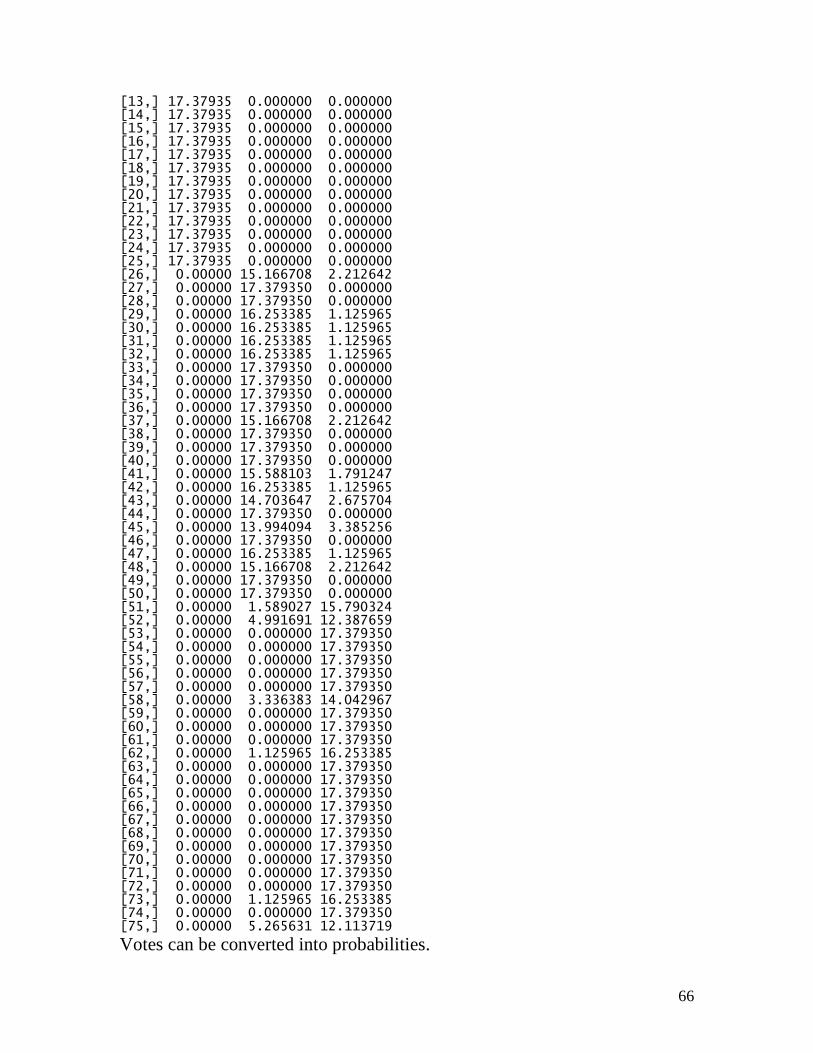
66

[13,] 17.37935 0.000000 0.000000 [14,] 17.37935 0.000000 0.000000 [15,] 17.37935 0.000000 0.000000 [16,] 17.37935 0.000000 0.000000 [17,] 17.37935 0.000000 0.000000 [18,] 17.37935 0.000000 0.000000 [19,] 17.37935 0.000000 0.000000 [20,] 17.37935 0.000000 0.000000 [21,] 17.37935 0.000000 0.000000 [22,] 17.37935 0.000000 0.000000 [23,] 17.37935 0.000000 0.000000 [24,] 17.37935 0.000000 0.000000 [25,] 17.37935 0.000000 0.000000 [26,] 0.00000 15.166708 2.212642 [27,] 0.00000 17.379350 0.000000 [28,] 0.00000 17.379350 0.000000 [29,] 0.00000 16.253385 1.125965 [30,] 0.00000 16.253385 1.125965 [31,] 0.00000 16.253385 1.125965 [32,] 0.00000 16.253385 1.125965 [33,] 0.00000 17.379350 0.000000 [34,] 0.00000 17.379350 0.000000 [35,] 0.00000 17.379350 0.000000 [36,] 0.00000 17.379350 0.000000 [37,] 0.00000 15.166708 2.212642 [38,] 0.00000 17.379350 0.000000 [39,] 0.00000 17.379350 0.000000 [40,] 0.00000 17.379350 0.000000 [41,] 0.00000 15.588103 1.791247 [42,] 0.00000 16.253385 1.125965 [43,] 0.00000 14.703647 2.675704 [44,] 0.00000 17.379350 0.000000 [45,] 0.00000 13.994094 3.385256 [46,] 0.00000 17.379350 0.000000 [47,] 0.00000 16.253385 1.125965 [48,] 0.00000 15.166708 2.212642 [49,] 0.00000 17.379350 0.000000 [50,] 0.00000 17.379350 0.000000 [51,] 0.00000 1.589027 15.790324 [52,] 0.00000 4.991691 12.387659 [53,] 0.00000 0.000000 17.379350 [54,] 0.00000 0.000000 17.379350 [55,] 0.00000 0.000000 17.379350 [56,] 0.00000 0.000000 17.379350 [57,] 0.00000 0.000000 17.379350 [58,] 0.00000 3.336383 14.042967 [59,] 0.00000 0.000000 17.379350 [60,] 0.00000 0.000000 17.379350 [61,] 0.00000 0.000000 17.379350 [62,] 0.00000 1.125965 16.253385 [63,] 0.00000 0.000000 17.379350 [64,] 0.00000 0.000000 17.379350 [65,] 0.00000 0.000000 17.379350 [66,] 0.00000 0.000000 17.379350 [67,] 0.00000 0.000000 17.379350 [68,] 0.00000 0.000000 17.379350 [69,] 0.00000 0.000000 17.379350 [70,] 0.00000 0.000000 17.379350 [71,] 0.00000 0.000000 17.379350 [72,] 0.00000 0.000000 17.379350 [73,] 0.00000 1.125965 16.253385 [74,] 0.00000 0.000000 17.379350 [75,] 0.00000 5.265631 12.113719

Votes can be converted into probabilities.

67

$prob [,1] [,2] [,3] [1,] 1 0.00000000 0.00000000 [2,] 1 0.00000000 0.00000000 [3,] 1 0.00000000 0.00000000 [4,] 1 0.00000000 0.00000000 [5,] 1 0.00000000 0.00000000 [6,] 1 0.00000000 0.00000000 [7,] 1 0.00000000 0.00000000 [8,] 1 0.00000000 0.00000000 [9,] 1 0.00000000 0.00000000 [10,] 1 0.00000000 0.00000000 [11,] 1 0.00000000 0.00000000 [12,] 1 0.00000000 0.00000000 [13,] 1 0.00000000 0.00000000 [14,] 1 0.00000000 0.00000000 [15,] 1 0.00000000 0.00000000 [16,] 1 0.00000000 0.00000000 [17,] 1 0.00000000 0.00000000 [18,] 1 0.00000000 0.00000000 [19,] 1 0.00000000 0.00000000 [20,] 1 0.00000000 0.00000000 [21,] 1 0.00000000 0.00000000 [22,] 1 0.00000000 0.00000000 [23,] 1 0.00000000 0.00000000 [24,] 1 0.00000000 0.00000000 [25,] 1 0.00000000 0.00000000 [26,] 0 0.87268557 0.12731443 [27,] 0 1.00000000 0.00000000 [28,] 0 1.00000000 0.00000000 [29,] 0 0.93521247 0.06478753 [30,] 0 0.93521247 0.06478753 [31,] 0 0.93521247 0.06478753 [32,] 0 0.93521247 0.06478753 [33,] 0 1.00000000 0.00000000 [34,] 0 1.00000000 0.00000000 [35,] 0 1.00000000 0.00000000 [36,] 0 1.00000000 0.00000000 [37,] 0 0.87268557 0.12731443 [38,] 0 1.00000000 0.00000000 [39,] 0 1.00000000 0.00000000 [40,] 0 1.00000000 0.00000000 [41,] 0 0.89693244 0.10306756 [42,] 0 0.93521247 0.06478753 [43,] 0 0.84604121 0.15395879 [44,] 0 1.00000000 0.00000000 [45,] 0 0.80521387 0.19478613 [46,] 0 1.00000000 0.00000000 [47,] 0 0.93521247 0.06478753 [48,] 0 0.87268557 0.12731443 [49,] 0 1.00000000 0.00000000 [50,] 0 1.00000000 0.00000000 [51,] 0 0.09143189 0.90856811 [52,] 0 0.28721967 0.71278033 [53,] 0 0.00000000 1.00000000 [54,] 0 0.00000000 1.00000000 [55,] 0 0.00000000 1.00000000 [56,] 0 0.00000000 1.00000000 [57,] 0 0.00000000 1.00000000 [58,] 0 0.19197399 0.80802601 [59,] 0 0.00000000 1.00000000 [60,] 0 0.00000000 1.00000000 [61,] 0 0.00000000 1.00000000 [62,] 0 0.06478753 0.93521247

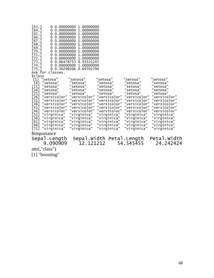
68

[63,] 0 0.00000000 1.00000000 [64,] 0 0.00000000 1.00000000 [65,] 0 0.00000000 1.00000000 [66,] 0 0.00000000 1.00000000 [67,] 0 0.00000000 1.00000000 [68,] 0 0.00000000 1.00000000 [69,] 0 0.00000000 1.00000000 [70,] 0 0.00000000 1.00000000 [71,] 0 0.00000000 1.00000000 [72,] 0 0.00000000 1.00000000 [73,] 0 0.06478753 0.93521247 [74,] 0 0.00000000 1.00000000 [75,] 0 0.30298206 0.69701794 Ask for classes. $class [1] "setosa" "setosa" "setosa" "setosa" "setosa" [6] "setosa" "setosa" "setosa" "setosa" "setosa" [11] "setosa" "setosa" "setosa" "setosa" "setosa" [16] "setosa" "setosa" "setosa" "setosa" "setosa" [21] "setosa" "setosa" "setosa" "setosa" "setosa" [26] "versicolor" "versicolor" "versicolor" "versicolor" "versicolor" [31] "versicolor" "versicolor" "versicolor" "versicolor" "versicolor" [36] "versicolor" "versicolor" "versicolor" "versicolor" "versicolor" [41] "versicolor" "versicolor" "versicolor" "versicolor" "versicolor" [46] "versicolor" "versicolor" "versicolor" "versicolor" "versicolor" [51] "virginica" "virginica" "virginica" "virginica" "virginica" [56] "virginica" "virginica" "virginica" "virginica" "virginica" [61] "virginica" "virginica" "virginica" "virginica" "virginica" [66] "virginica" "virginica" "virginica" "virginica" "virginica" [71] "virginica" "virginica" "virginica" "virginica" "virginica"

$importance Sepal.Length Sepal.Width Petal.Length Petal.Width 9.090909 12.121212 54.545455 24.242424 attr(,"class") [1] "boosting"

69

Classification Protocol Petal.Length < 2.5 setosa 2.5 ≤ Petal.Length < 4.9 and Petal.Width < 1.65 versicolor Petal.Length ≥ 4.9 and Petal.Width < 1.65 virginica 2.5 ≤ Petal.Length and Petal.Width < 1.65 virginica Confusion matrix True Status Tree Judgment setosa versicolor virginica Total setosa 25 0 0 25 versicolor 0 24 1 25 virginica 0 0 25 25 Misclassification rate = 1/75 = 1.3% Back to the boosting … > barplot(Boost$imp[order(Boost$imp, decreasing = T)], ylim = c(0, 100), + main = "Variables Relative Importance", col = "lightblue")

|Petal.Length< 2.5

Petal.Width< 1.65

Petal.Length< 4.9

setosa 25/25/25

setosa 25/0/0

versicolor0/25/25

versicolor0/25/2

versicolor0/24/0

virginica 0/1/2

virginica 0/0/23

Classification Tree of Iris data Randomly Chosen

Size = 75

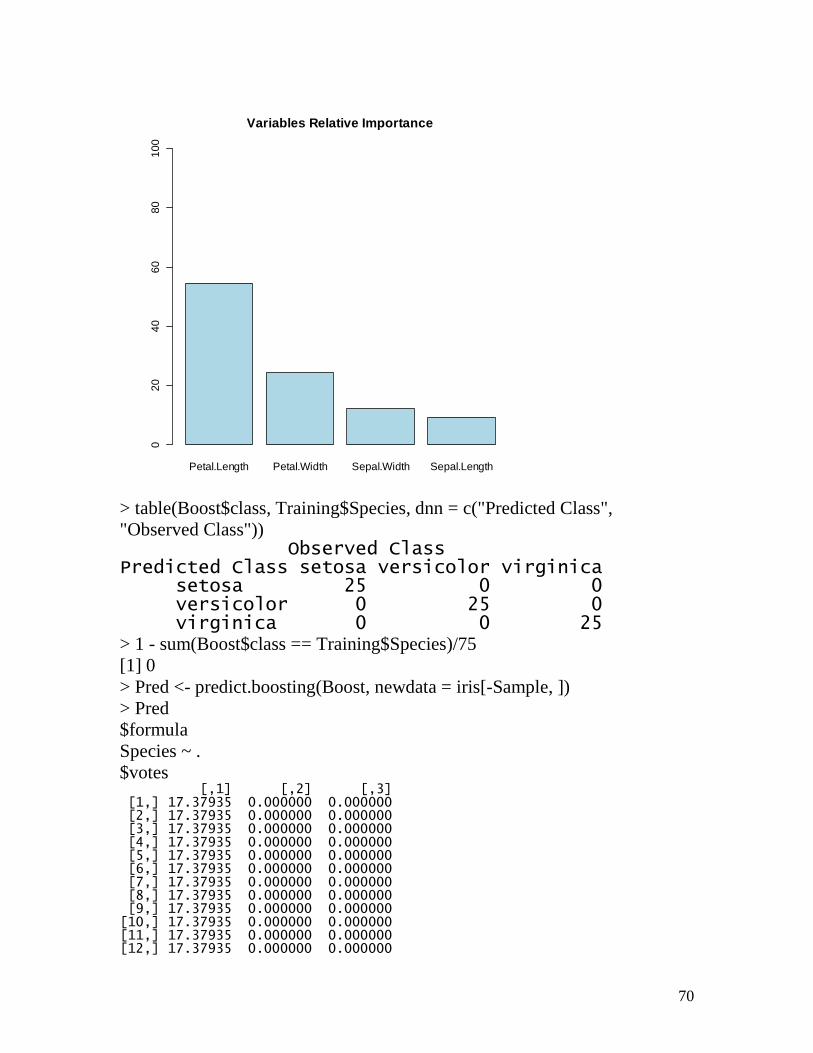
70

> table(Boost$class, Training$Species, dnn = c("Predicted Class", "Observed Class")) Observed Class Predicted Class setosa versicolor virginica setosa 25 0 0 versicolor 0 25 0 virginica 0 0 25 > 1 - sum(Boost$class == Training$Species)/75 [1] 0 > Pred <- predict.boosting(Boost, newdata = iris[-Sample, ]) > Pred $formula Species ~ . $votes [,1] [,2] [,3] [1,] 17.37935 0.000000 0.000000 [2,] 17.37935 0.000000 0.000000 [3,] 17.37935 0.000000 0.000000 [4,] 17.37935 0.000000 0.000000 [5,] 17.37935 0.000000 0.000000 [6,] 17.37935 0.000000 0.000000 [7,] 17.37935 0.000000 0.000000 [8,] 17.37935 0.000000 0.000000 [9,] 17.37935 0.000000 0.000000 [10,] 17.37935 0.000000 0.000000 [11,] 17.37935 0.000000 0.000000 [12,] 17.37935 0.000000 0.000000

Petal.Length Petal.Width Sepal.Width Sepal.Length

Variables Relative Importance

020

4060

8010

0

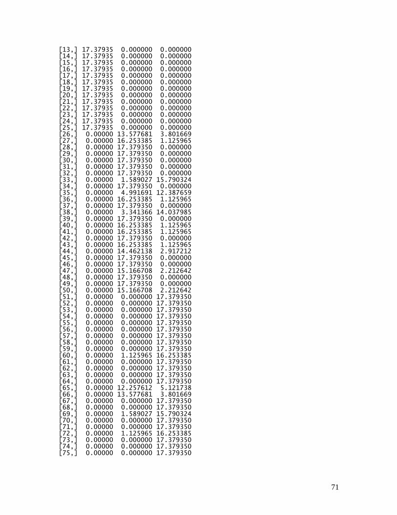
71

[13,] 17.37935 0.000000 0.000000 [14,] 17.37935 0.000000 0.000000 [15,] 17.37935 0.000000 0.000000 [16,] 17.37935 0.000000 0.000000 [17,] 17.37935 0.000000 0.000000 [18,] 17.37935 0.000000 0.000000 [19,] 17.37935 0.000000 0.000000 [20,] 17.37935 0.000000 0.000000 [21,] 17.37935 0.000000 0.000000 [22,] 17.37935 0.000000 0.000000 [23,] 17.37935 0.000000 0.000000 [24,] 17.37935 0.000000 0.000000 [25,] 17.37935 0.000000 0.000000 [26,] 0.00000 13.577681 3.801669 [27,] 0.00000 16.253385 1.125965 [28,] 0.00000 17.379350 0.000000 [29,] 0.00000 17.379350 0.000000 [30,] 0.00000 17.379350 0.000000 [31,] 0.00000 17.379350 0.000000 [32,] 0.00000 17.379350 0.000000 [33,] 0.00000 1.589027 15.790324 [34,] 0.00000 17.379350 0.000000 [35,] 0.00000 4.991691 12.387659 [36,] 0.00000 16.253385 1.125965 [37,] 0.00000 17.379350 0.000000 [38,] 0.00000 3.341366 14.037985 [39,] 0.00000 17.379350 0.000000 [40,] 0.00000 16.253385 1.125965 [41,] 0.00000 16.253385 1.125965 [42,] 0.00000 17.379350 0.000000 [43,] 0.00000 16.253385 1.125965 [44,] 0.00000 14.462138 2.917212 [45,] 0.00000 17.379350 0.000000 [46,] 0.00000 17.379350 0.000000 [47,] 0.00000 15.166708 2.212642 [48,] 0.00000 17.379350 0.000000 [49,] 0.00000 17.379350 0.000000 [50,] 0.00000 15.166708 2.212642 [51,] 0.00000 0.000000 17.379350 [52,] 0.00000 0.000000 17.379350 [53,] 0.00000 0.000000 17.379350 [54,] 0.00000 0.000000 17.379350 [55,] 0.00000 0.000000 17.379350 [56,] 0.00000 0.000000 17.379350 [57,] 0.00000 0.000000 17.379350 [58,] 0.00000 0.000000 17.379350 [59,] 0.00000 0.000000 17.379350 [60,] 0.00000 1.125965 16.253385 [61,] 0.00000 0.000000 17.379350 [62,] 0.00000 0.000000 17.379350 [63,] 0.00000 0.000000 17.379350 [64,] 0.00000 0.000000 17.379350 [65,] 0.00000 12.257612 5.121738 [66,] 0.00000 13.577681 3.801669 [67,] 0.00000 0.000000 17.379350 [68,] 0.00000 0.000000 17.379350 [69,] 0.00000 1.589027 15.790324 [70,] 0.00000 0.000000 17.379350 [71,] 0.00000 0.000000 17.379350 [72,] 0.00000 1.125965 16.253385 [73,] 0.00000 0.000000 17.379350 [74,] 0.00000 0.000000 17.379350 [75,] 0.00000 0.000000 17.379350

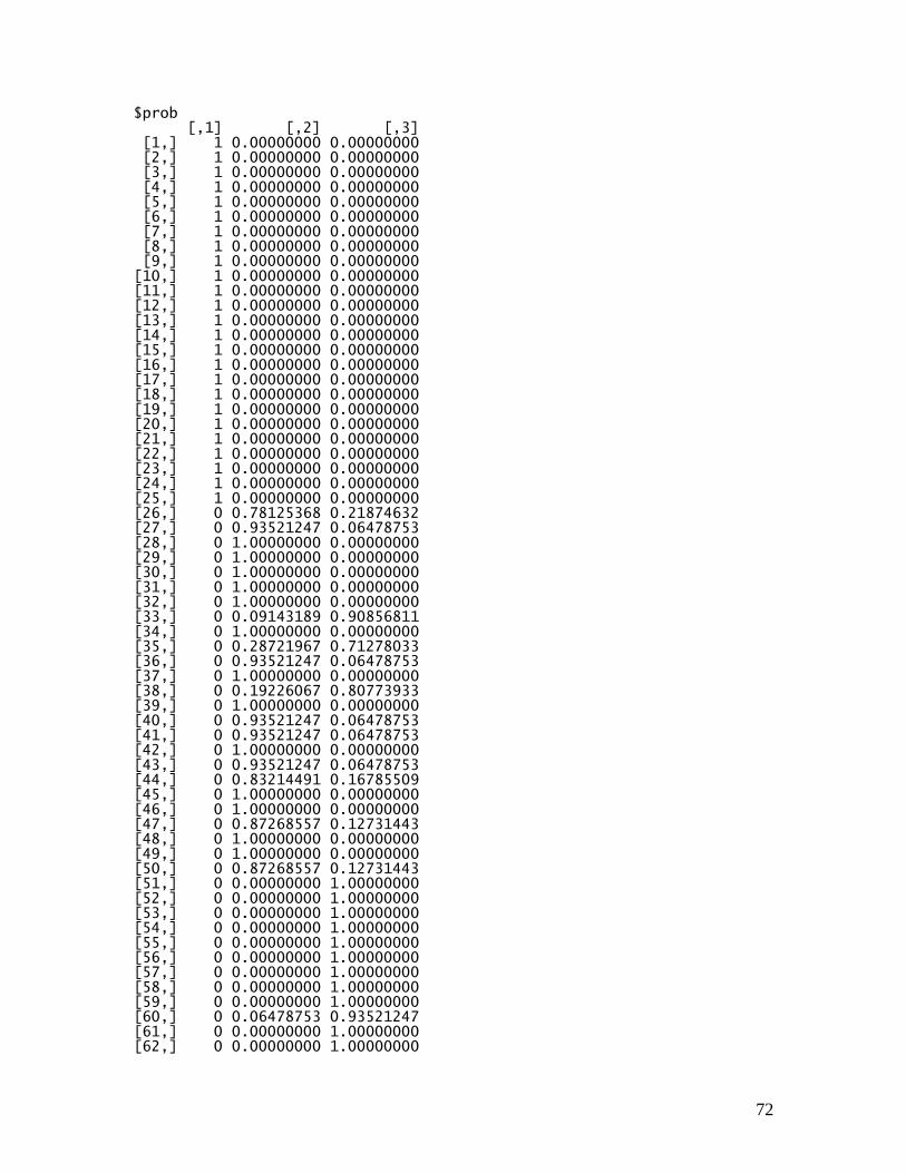
72

$prob [,1] [,2] [,3] [1,] 1 0.00000000 0.00000000 [2,] 1 0.00000000 0.00000000 [3,] 1 0.00000000 0.00000000 [4,] 1 0.00000000 0.00000000 [5,] 1 0.00000000 0.00000000 [6,] 1 0.00000000 0.00000000 [7,] 1 0.00000000 0.00000000 [8,] 1 0.00000000 0.00000000 [9,] 1 0.00000000 0.00000000 [10,] 1 0.00000000 0.00000000 [11,] 1 0.00000000 0.00000000 [12,] 1 0.00000000 0.00000000 [13,] 1 0.00000000 0.00000000 [14,] 1 0.00000000 0.00000000 [15,] 1 0.00000000 0.00000000 [16,] 1 0.00000000 0.00000000 [17,] 1 0.00000000 0.00000000 [18,] 1 0.00000000 0.00000000 [19,] 1 0.00000000 0.00000000 [20,] 1 0.00000000 0.00000000 [21,] 1 0.00000000 0.00000000 [22,] 1 0.00000000 0.00000000 [23,] 1 0.00000000 0.00000000 [24,] 1 0.00000000 0.00000000 [25,] 1 0.00000000 0.00000000 [26,] 0 0.78125368 0.21874632 [27,] 0 0.93521247 0.06478753 [28,] 0 1.00000000 0.00000000 [29,] 0 1.00000000 0.00000000 [30,] 0 1.00000000 0.00000000 [31,] 0 1.00000000 0.00000000 [32,] 0 1.00000000 0.00000000 [33,] 0 0.09143189 0.90856811 [34,] 0 1.00000000 0.00000000 [35,] 0 0.28721967 0.71278033 [36,] 0 0.93521247 0.06478753 [37,] 0 1.00000000 0.00000000 [38,] 0 0.19226067 0.80773933 [39,] 0 1.00000000 0.00000000 [40,] 0 0.93521247 0.06478753 [41,] 0 0.93521247 0.06478753 [42,] 0 1.00000000 0.00000000 [43,] 0 0.93521247 0.06478753 [44,] 0 0.83214491 0.16785509 [45,] 0 1.00000000 0.00000000 [46,] 0 1.00000000 0.00000000 [47,] 0 0.87268557 0.12731443 [48,] 0 1.00000000 0.00000000 [49,] 0 1.00000000 0.00000000 [50,] 0 0.87268557 0.12731443 [51,] 0 0.00000000 1.00000000 [52,] 0 0.00000000 1.00000000 [53,] 0 0.00000000 1.00000000 [54,] 0 0.00000000 1.00000000 [55,] 0 0.00000000 1.00000000 [56,] 0 0.00000000 1.00000000 [57,] 0 0.00000000 1.00000000 [58,] 0 0.00000000 1.00000000 [59,] 0 0.00000000 1.00000000 [60,] 0 0.06478753 0.93521247 [61,] 0 0.00000000 1.00000000 [62,] 0 0.00000000 1.00000000

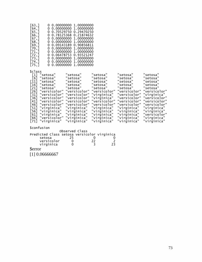
73

[63,] 0 0.00000000 1.00000000 [64,] 0 0.00000000 1.00000000 [65,] 0 0.70529750 0.29470250 [66,] 0 0.78125368 0.21874632 [67,] 0 0.00000000 1.00000000 [68,] 0 0.00000000 1.00000000 [69,] 0 0.09143189 0.90856811 [70,] 0 0.00000000 1.00000000 [71,] 0 0.00000000 1.00000000 [72,] 0 0.06478753 0.93521247 [73,] 0 0.00000000 1.00000000 [74,] 0 0.00000000 1.00000000 [75,] 0 0.00000000 1.00000000 $class [1] "setosa" "setosa" "setosa" "setosa" "setosa" [6] "setosa" "setosa" "setosa" "setosa" "setosa" [11] "setosa" "setosa" "setosa" "setosa" "setosa" [16] "setosa" "setosa" "setosa" "setosa" "setosa" [21] "setosa" "setosa" "setosa" "setosa" "setosa" [26] "versicolor" "versicolor" "versicolor" "versicolor" "versicolor" [31] "versicolor" "versicolor" "virginica" "versicolor" "virginica" [36] "versicolor" "versicolor" "virginica" "versicolor" "versicolor" [41] "versicolor" "versicolor" "versicolor" "versicolor" "versicolor" [46] "versicolor" "versicolor" "versicolor" "versicolor" "versicolor" [51] "virginica" "virginica" "virginica" "virginica" "virginica" [56] "virginica" "virginica" "virginica" "virginica" "virginica" [61] "virginica" "virginica" "virginica" "virginica" "versicolor" [66] "versicolor" "virginica" "virginica" "virginica" "virginica" [71] "virginica" "virginica" "virginica" "virginica" "virginica" $confusion Observed Class Predicted Class setosa versicolor virginica setosa 25 0 0 versicolor 0 22 2 virginica 0 3 23

$error [1] 0.06666667

BOOTSTRAP AND APPLICATIONS - crrao AND APPLICATIONS ... Nonparametric Regression + Classification...

Documents

Transcript of BOOTSTRAP AND APPLICATIONS - crrao AND APPLICATIONS ... Nonparametric Regression + Classification...